ncube, matiwaza (2012) the development of a methodology ... · project. to my main supervisor,...
TRANSCRIPT

Ncube, Matiwaza (2012) The development of a methodology for a tool for rapid assessment of indoor environment quality in office buildings in the UK. PhD thesis, University of Nottingham.
Access from the University of Nottingham repository: http://eprints.nottingham.ac.uk/12492/1/Doctor_Thesis_for_Submission.pdf
Copyright and reuse:
The Nottingham ePrints service makes this work by researchers of the University of Nottingham available open access under the following conditions.
· Copyright and all moral rights to the version of the paper presented here belong to
the individual author(s) and/or other copyright owners.
· To the extent reasonable and practicable the material made available in Nottingham
ePrints has been checked for eligibility before being made available.
· Copies of full items can be used for personal research or study, educational, or not-
for-profit purposes without prior permission or charge provided that the authors, title and full bibliographic details are credited, a hyperlink and/or URL is given for the original metadata page and the content is not changed in any way.
· Quotations or similar reproductions must be sufficiently acknowledged.
Please see our full end user licence at: http://eprints.nottingham.ac.uk/end_user_agreement.pdf
A note on versions:
The version presented here may differ from the published version or from the version of record. If you wish to cite this item you are advised to consult the publisher’s version. Please see the repository url above for details on accessing the published version and note that access may require a subscription.
For more information, please contact [email protected]
The Development of a Methodology for a Tool for Rapid Assessment of Indoor
Environment Quality in Office Buildings in the UK
Matiwaza Ncube
Bsc (Hons), Msc.
Thesis submitted to the University of Nottingham for the degree of Doctor of Philosophy
March 2012

i
Preface
“Diamonds resist blows to such an extent that an iron hammer may be split in two
and even the anvil itself may be displaced. This invincible force, which defies
Nature's two most violent forces, iron and fire, can be broken by ram's blood. But it
must be steeped in blood that is fresh and warm and, even so, many blows are
needed." - PLINY THE ELDER

ii
Abstract
This thesis describes a methodology for the development of a novel tool for rapid assessment
of Indoor Environment Quality (IEQ) in office buildings in the UK. The tool uses design,
measured, calculated and surveyed data as input for IEQ calculations. The development of such
a tool has become a necessity especially in the developed world where legally binding targets
for Green House Gas (GHG) emissions have been agreed and where buildings are required by
law to display energy performance certification. The novelty of this tool is that it addresses the
need to present an indoor environment performance rating that can be presented alongside
energy performance certification since the energy performance of office buildings depends
significantly on the criteria used for the indoor environment.
The tool, called the IEQAT (Indoor Environment Quality Assessment Tool), is based on the
IEQ model which was developed from literature review. The IEQ model is based on the IEQ
index which was derived from contributing factors or sub indices that include Thermal
Comfort, Indoor Air quality (IAQ), Acoustic Comfort and Lighting. The model was tested by
studying the responses of occupants of three office buildings in the UK. Their subjective
responses which were collected via a questionnaire were compared against model simulation
results which were calculated using physical measurements of IEQ variables such as air
temperature, illuminance (lux), background noise levels (dBA), relative humidity, carbon
dioxide concentration (ppm), and air velocity. By fitting a multivariate regression model to
questionnaire data, a weighted ranking of parameters affecting IEQ was produced and new
provisional weightings for the IEQ model, which is more relevant to the UK situation, were
derived.

iii
Acknowledgements
This thesis is dedicated to my daughters Wendy and Lisani and to my parents.
I would like to express my sincere gratitude to the following people for their support and
guidance. First, I would like to thank Prof. Xudong Zhao (De Montfort University) for his help,
support and guidance during the initial part of the work. I would also like to thank Prof.
Cees van der Eijk of the Methods and Data Institute (Nottingham University) for his input
during study and questionnaire design. Many thanks also go to Dr. Nelson Chilengwe and Nick
Cullen of Hoare Lea and Partners for their continued support during the entire duration of the
project.
To my main supervisor, Prof. Saffa Riffat I would like to say Thank you for your support,
guidance and project supervision. I would like to thank the EPSRC and Hoare Lea & Partners
for their financial support. Thank you also to Hoare Lea - Leeds Office, Marsh Growchoski &
Associates and Hestia Managed Services for giving me the opportunity to use their offices for
data collection purposes. Many thanks go to my family especially my partner for their patience,
understanding and encouragement. Thank you especially to my University for giving me the
opportunity.

iv
Table of Contents
Preface……………………………………………………………………………………..…...i
Abstract…………………………………………………………………………………...…...ii
Acknowledgements………………...………………………….……………………………….iii
Table of Contents…………………...…………………………….……………………………iv
List of Figures………………………...……………………………………………………....viii
List of Tables………………………..………………………………………………………..xiii
Nomenclature…………………………..….…………………………………………………..xv
1. Introduct ion………………………..….……………………………………………………..1
1.1 BACKGROUND………………….……………………………………………………..1
1.2 AIMS AND OBJECTIVES OF THE STUDY……...……….......................................9
1.3 OUTLINE OF THE THESIS……………………...……………………………….......11
2. Literature Review……………………………………………..……….…………………..14
2.1 ENERGY USE IN OFFICE BUILDINGS IN THE UK……..…….…………………..14
2.1.1 Major End Uses………………………………………...………………………14
2.1.2 Strategies to Reduce Energy Use………………………………………….21
2.2 THE INDOOR ENVIRONMENT…………………………..………………………….25
2.2.1 Introduction…………………………………………..………………………25
2.2.2 Overview of IEQ Assessment in Office Buildings...…...……………………25
2.2.3 Current IEQ Assessment Tools………………………………………..……..29
2.3 THE THERMAL ENVIRONMENT………………………………………….………..31
2.3.1 Overview of the Thermal Environment Assessment in Office Buildings...31
2.4 INDOOR AIR QUALITY………………………..…………………………….………37
2.4.1 Air Quality problems in buildings ……..……………………………………37
2.4.2 Overview of IAQ Assessment in Office Buildings…………….................40
2.4.3 Sources of Pollution in Offices ………………………………….…………..42
2.4.4 The Sick Building Syndrome ……………………………….……………….43
2.5 THE ACOUSTIC ENVIRONMENT……………………………………..……………43
2.5.1 Overview of the Acoustic Comfort Evaluation in Offices..................................43
v
2.6 LIGHTING (VISUAL) COMFORT………………………………………… ………..47
2.6.1 Overview of Lighting in Office Buildings…………………………………….47
2.7 CURRENT STANDARDS IN THE OPERATION OF OFFICES……………….....50
2.7.1 Criteria For Thermal Operation of Mechanically Ventilated Buildings.….50
2.7.2 Criteria For Thermal Operation of Naturally Ventilated Buildings - Adaptive
Comfort……………………………………………….……...............................59
2.7.3 IAQ and Ventilation Standards…………………………….……...............60
2.7.4 Criteria for Acoustics Operation of Offices..... 63
2.7.5 Lighting Recommendations in Office Buildings……………………..….......64
2.8 Conclusions……………………………………………………………………..……...68
3. The IEQ Assessment Model………………………………………………………….....70
3.1 IMPORTANT FEATURES OF THE IEQAT ASSESSMENT METHODOLOGY…..70
3.2 DEVELOPMENT SOFTWARE…………………………………………………...…..71
3.3 DEVELOPING THE ASSESSMENT MODEL………………………………...……..72
3.3.1 Development of Thermal Comfort Sub-Index…………………..……...............72
3.3.2 Development of IAQ Sub-Index………………………………….…….........82
3.3.3 Development of the Acoustic Comfort Sub-Index…………………..….......87
3.3.4 Development of Lighting Quality Sub-Index……………………….……….91
3.3.5 Development of Perceived IEQ Index and the relative weightings….…....93
3.4 ENERGY PERFORMANCE ASSESSMENT METHODOLOGIES ... ..99
3.5 THE IEQAT..103
3.5.1 Data Input .. 105
3.5.2 Assessment Results Sheets116
3.5.3 Long Term Indicators of IEQ and Recommended Criteria for Acceptable
Deviation and Length of Deviation from Standard Conditions.119
3.6 Conclusions... .124
4. Research Methodology ... 125
4.1 RESEARCH DESIGN …...125
4.1.1 Selection of Research Design 125
vi
4.1.2 The Methodological Basis of Correlational Designs.129
4.1.3 The Design Notation..131
4.2 SELECTION OF SAMPLE BUILDINGS 133
4.3 DATA COLLECTION EXERCISE - THE QUESTIONNAIRE ..137
4.3.1 Motivation for the Questionnaire...137
4.3.2 Questionnaire Structure.141
4.4 DATA COLLECTION EXERCISE – PHYSICAL MEASUREMENTS .145
4.4.1 Parameters to Measure ..146
4.4.2 Data Collection Exercise and Equipment Used.149
4.4.3 Monitoring Layout & Positioning of Sensors ...160
5. Results & Tool Evaluation... ..163
5.1 CASE STUDY 1: LEEDS TOWN CENTRE HOUSE, LEEDS ...163
5.1.1 Thermal Comfort Assessment Results...........165
5.1.2 Indoor air Quality Assessment Results..........175
5.1.3 Acoustic Comfort Assessment Results.........176
5.1.4 Lighting Quality Assessment Results 177
5.1.5 IEQ Assessment Results 180
5.1.6 Long Term Evaluation of IEQ – Model Performance...181
5.1.7 General Considerations for the Indoor Environment.185
5.1.8 Conclusions and lessons learnt from the study..186
5.2 CASE STUDY 2: MARSH GROWCHOSKI & ASSOCIATES, NOTTINGHAM.187
5.2.1 Thermal Comfort Assessment Results...........189
5.2.2 Indoor Air Quality Assessment Results .195
5.2.3 Acoustic Comfort Assessment Results..198
5.2.4 Lighting Quality Assessment Results 199
5.2.5 IEQ Assessment Results 201
5.2.6 Long Term Evaluation Capabilities of the IEQ Model..203
5.2.7 General Considerations for the Indoor Environment.207
5.2.8 Conclusions and lessons learnt from the study..207
vii
5.3 CASE STUDY 3: GRANBY HOUSE, NOTTINGHAM .208
5.3.1 Thermal, IAQ, Acoustic and Lighting Comfort Assessment Results210
5.3.2 IEQ Assessment Results for the Granby House....212
5.3.3 General Checklist of the Granby House Office Space..214
5.3.4 Conclusions & Lessons Learnt from the Case Study............215
5.4 MULTIVARIATE REGRESSION ANALYSIS ...215
5.5 CONCLUIONS...........................................................................................................218
6. Discussion of the Tool, Suggestions for Future Work and Conclusions 220
6.1 GENERAL DISCUSSION & SUGGESTED IMPROVEMENTS OF IEQAT
INDICES ... 220
6.1.1 Thermal Comfort Index .222
6.1.2 IAQ index ..229
6.1.3 Lighting Comfort Index .231
6.1.4 Acoustic Comfort Index .233
6.1.5 Important features of the IEQAT...235
6.2 GENERAL CONCLUSIONS 237
6.2.1 IEQ indices ..238
6.2.2 The case study buildings.239
6.2.3 The IEQ Model………………………………………………………....241
6.3 RECOMMENDATIONS FOR FUTURE RESEARCH...241
7. References ...244
8. Appendices: 257
Appendix 1 The Visual basic code for thermal comfort calculation256
Appendix 2 The Indoor Environment Questionnaire…...262
Appendix 3 The IEQAT Assessment Results for the Leeds Town Centre House; Marsh
Grochowski & Associates, and the Granby House.269
Appendix 4 A plot of % acceptance against operative temperatures……………...............272
Appendix 5 List of Work Published in Journals & Conference Proceedings...............272
viii
List of Figures
Figure 1.1 Global Temperature Change Estimated at the Surface, Over the Period 1880 to
2010………………………………………………………………………2
Figure 1.2 Global Installed Power Generation Capacity and Additions by Technology .3
Figure 1.3 Actual and Predicted Carbon Dioxide Emissions by Region, 1990 – 2030 4
Figure 1.4 World Marketed Energy Consumption, 1980 – 2030, Adapted from the International
Energy Outlook, 2006……5
Figure 1.5 Energy Consumption by Sector in Primary Energy Equivalents 1970 to 2010,
UK…………………………………………………………………………..............6
Figure 1.6 Flowchart: The development of a Methodology for Assessment of IEQ in Office
Buildings …..11
Figure 2.1 Growth in commercial office floor space in England and Wales 1970 to
2000 ..21
Figure 2.2 Main Constituents of Stimulus in Indoor Microclimate................26
Figure 2.3 The Cylindrical Model of Thermal Interaction of Human Body and the
Environment .....32
Figure 2.4 Air velocity required to offset increase in air Temperature, Adapted from (EN15251,
2006) ………………………………………………………………...54
Figure 2.5 Illustration of a ventilation system of a centrally conditioned
space ……………………………………………………………….....55
Figure 2.6 Illustration of a dehumidification system that involves cooling air below dew
point …….57
Figure 2.7 Desiccant based dehumidification system….58
Figure 2.8 Recommended design indoor operative temperatures for naturally ventilated offices
in the UK ..59
Figure 2.9 Task area & immediate surrounding area…....65
Figure 3.1 Thermal Comfort Estimation Flowchart ………………………………………..74
Figure 3.2 Predicted Percentage Dissatisfied Plotted Against PMV Values…………..80

ix
Figure 3.3 Percentage Dissatisfied (caused by one person, 1olf) Plotted against Ventilation
Rates in l/s…………………………………………………………....85
Figure 3.4 Plot of PD versus Measured CO2 Concentration above Outdoor Concentrations
…………………………………………………………………..85
Figure 3.5 Relationships between Perceived Air Quality Expressed by the Percentage of
Dissatisfied and Expressed in Decipol…………………………………….86
Figure 3.6 IAQ Estimation Flowchart……………………………………………………….87
Figure 3.7 A-weighted Equivalent Sound Levels Against % Complaints………………..88
Figure 3.8 Relationship between background noise level (dBA) and comments likely to be
obtained from room occupants …………………………………………................89
Figure 3.9 Acoustic Comfort Estimation Flowchart………………………………………...90
Figure 3.10 Plot of ln(ln (lux)) Against Quality of Lighting………………………………..92
Figure 3.11 Lighting Comfort Estimation Flowchart…………………………………….........93
Figure 3.12 Illustration of the Logistic Function Curve………………………………….97
Figure 3.13 IEQ Estimation Flowchart……………………………………………………...98
Figure 3.14 Summary of the Variables Used for IEQ and Energy Calculations……..100
Figure 3.15 Energy Performance Certificate Showing a D rated domestic building................103
Figure 3.16 Flowchart of IEQ Calculation Steps………………………………………..104
Figure 3.17 Data Entry Sheet 1/1– Project and Building Data……………………….............105
Figure 3.18 Data Entry Sheet 2 of 1……………………………………………………..........108
Figure 3.19 Data Entry Sheet 2………………………………………………………….........108
Figure 3.20 Data Entry Sheet 3 - Thermal Comfort Factors and General Checklist Record
Sheet…………………………………………………………………...112
Figure 3.21 Data Entry Sheet 4 - IAQ Factors and General Considerations Record
Sheet……………………………………………………………………………...113
Figure 3.22 Data Entry Sheet 5 – Acoustic Comfort Factors and General Considerations
Record Sheet………………………………………………..................................114
Figure 3.23 Data Entry Sheet 6 – Lighting Comfort Factors and General Considerations Record
Sheet………………………………………………...............................................115
Figure 3.24 Assessment Results Sheet 1………………………………………………...116
Figure 3.25 Assessment Results Sheet 2………………………………………………...117
Figure 3.26 Comparisons between Energy and IEQ Ratings for Typical Office……..118
x
Figure 3.27 Assessment Results Sheet Showing % of time Office Space falls into a particular
Category…………………………………………………………….122
Figure 3.28 Real time or Long term representation of Office Assessment results…...123
Figure 3.29 Methodology for Assessment of Multiple Offices…………………………124
Figure 4.1 Categories of Research Designs……………………………………………..126
Figure 4.2 Methodological Basis of Correlational Studies……………………………...131
Figure 4.3 Design Notation for Occupant Exposure to IEQ Conditions………………..132
Figure 4.4 Diagram Showing Typical Layout of the Working Plane…………………...145
Figure 4.5 The Datataker DT 500 3 Series data logger……………………………….150
Figure 4.6 The T Type Thermocouple from RS instruments…………………………151
Figure 4.7 The SKL 2630 Lux Sensor, from Skye Instruments………………………...152
Figure 4.8 The Vaisala FMA-1000 CO2 transmitter……………………………………153
Figure 4.9 The Hagner digital Lux Meter………………………………………………........154
Figure 4.10 The 4 in 1 Multifunction Environment meter………………………………155
Figure 4.11 Hand held Humidity and Temperature Probe meter…………………….............157
Figure 4.12 Typical Data Logging Set Up………………………………………………157
Figure 4.13 Picture of the Data Logging Set Up………………………………………..........158
Figure 4.14 Typical program builder window…………………………………………..........159
Figure 4.15 Typical Software Interface…………………………………………………160
Figure 4.16 Typical Office Divided into Sections, Zones and Positions………………..161
Figure 4.17 Data Collection Set Up on a Working Plane……………………………….161
Figure 5.1 Project and Building Data – Town Centre House – Leeds………………..164
Figure 5.2 Population Distributions by age of the occupants of the 6th Floor Office..167
Figure 5.3 Surveyed Vs Calculated PMV Values – LTCH……………………………..168
Figure 5.4 Calculated vs. Surveyed Thermal Comfort Values across Office Space –
LTCH…………………………………………………………………………….169
Figure 5.5 Frequency Distribution of PMV Values for Sections A and B – LTCH…............169
Figure 5.6 Day 1, Section A - Zone 1, Temperature Profiles (DT500) – LTCH…….............171
Figure 5.7 Recorded Mean Temperatures – LTCH……………………………………..172
Figure 5.8 Temperature Difference with Increasing Height of Sensor above Floor Level
(DT500) – LTCH………………………………………………………………...173

xi
Figure 5.9 Day Two, Section B - Zone 1, recorded air velocities (DT500) – LTCH…..174
Figure 5.10 CO2 Concentration Profile, Day 3 (DT500) – LTCH……………………..175
Figure 5.11 Surveyed Vs Predicted IAQ Perception in the Office – LTCH…………176
Figure 5.12 Surveyed Vs Calculated Acoustic Comfort Values – LTCH……………177
Figure 5.13 Day 2, Section A, Illuminance (DT500) – LTCH………………………….178
Figure 5.14 Surveyed Vs Calculated Lighting Quality Values – LTCH………………..179
Figure 5.15 Level of Agreement of Responses Obtained from the Semantic Differential and the
Visual Analogue Scales (VAS)……………………………………......................179
Figure 5.16 Picture of Indoor Environment – LTCH……………………………………180
Figure 5.17 Surveyed Vs Model Calculated IEQ values – LTCH……………………181
Figure 5.18 Assessment Results – Section A, Line Graph Presentation – LTCH…182
Figure 5.19 Average Results for Section A of the Leeds Town Centre House 6th Floor Office
Space……………………………………………………………………..183
Figure 5.20 Percentage of Time Office Falls Inside the Limits of a Category –
LTCH…………………………………………………………………………….184
Figure 5.21 Project and Building Data – Marsh Grochowski & Associates – Nottingham
…………………………………………………………………………………...188
Figure 5.22 Calculated vs. Surveyed PMV values for the 2nd Floor, Marsh & Grochowski
Architects, Nottingham…………………………………………..190
Figure 5.23 Calculated vs. Surveyed PMV values for the 3rd Floor, Marsh & Grochowski
Architects – Nottingham………………………………………191
Figure 5.24 Frequency distribution of PMV values for the Marsh & Grochowski Architects,
Nottingham……………………………………………………….192
Figure 5.25 Model vs Surveyed PMV values for the Marsh, Grochowski & Associates -
Nottingham…………………………………………………………………….192
Figure 5.26 Temperature Profile for the Top (third) Floor Section of the Office Building
(DT500) – MGA………………………………………………………………....193
Figure 5.27 Temperature Profiles at Various Locations in the Office – MGA……….194
Figure 5.28 Recorded Air Velocities – Second Floor Marsh & Grochowski Architects,
Nottingham (DT500)…………………………………………………………..195
xii
Figure 5.29 CO2 Concentrations over a 24hr Period in the Third Floor of the Office Building
(DT500) – MGA………………………………………………………196
Figure 5.30 Calculated vs. Surveyed Acceptance of IAQ – MGA……………………...197
Figure 5.31 Surveyed Vs Calculated Acoustics Acceptance, 2nd & 3rd Floor –
MGA……………………………………………………………………………..199
Figure 5.32 Logged Illuminance on a Working Plane Second Floor Office Space (DT500) –
MGA………………………………………………………………......................200
Figure 5.33 Logged Illuminance on a Working Plane Third Floor Office Space (DT500) –
MGA…………………………………………………………………………..200
Figure 5.34 Calculated vs. Observed acceptance of lighting in the offices –MGA….201
Figure 5.35 Top floor office design, furniture levels, etc – MGA………………………202
Figure 5.36 Calculated vs. Surveyed IEQ – MGA………………………………………...203
Figure 5.37 Assessment results for period 11:30 – 14:00 – Line Graph
(Marsh & Growchoski)…………………………………………………………………….204
Figure 5.38 Average assessment results for the period 11:30 – 14:00 - radar chart –
MGA……………………………………………………………………………..205
Figure 5.39 Long term assessment results – Bar graph representation – MGA……...206
Figure 5.40 Project and building data – Granby House – Nottingham City Centre….209
Figure 5.41 Comparison between Model calculated and Survey results -– GH……………...211
Figure 5.42 Comparison between Model calculated and Survey IEQ results - GH…….....212
Figure 5.43 Radar chart – Overall IEQ rating Granby House…………………………...212
Figure 5.44 Bar Graph - Overall IEQ rating of the Granby House office……………213
Figure 6.1 Local Discomfort Caused by radiant Temperature Asymmetry…………..224
Figure 6.2 Effects of changes in air and mean radiant temperature on IEQ ratings.226
Figure 6.3 Effects of Air Velocity on IEQ………………………………………………........227
Figure 6.4 Effects of Relative Humidity on IEQ…………………………………………..228
Figure 6.5 Effects of Indoor CO2 Concentrations on IEQ……………………………...230
Figure 6.6 Effects of illuminance on IEQ………………………………………………….232
Figure 6.7 Effects of Background noise level on IEQ…………………………………..234
xiii
List of Tables
Table 2.1 Energy Use in the Commercial Sector by Building Type.. .14
Table 2.2 Energy Use in Offices by End use…..16
Table 2.3 Proportion of Energy Consumption in Offices by End Use... ........16
Table 2.4 Energy consumption and CO2 emissions in UK Commercial Offices…...17
Table 2.5 Typical and Good Practice Energy Consumption in Offices in the UK... ..19
Table 2.6 Seven Point ASHRAE Thermal Sensation Scale ...……33
Table 2.7 Design values for different types of offices spaces ... .45
Table 2.8 Comparison of Noise Weighting Curves for Purposes of Evaluation the Indoor
Acoustic Environments46
Table 2.9 Thermal Comfort Categories for Offices.51
Table 2.10 Examples of Recommended Indoor Temperature Design Values for Buildings and
HVAC Systems ... .51
Table 2.11 Example of recommended design criteria for the humidity in occupied spaces where
humidification or dehumidification systems are Installed…...58
Table 2.12 Air Quality Categories Based on Amount of Ventilation Air Supplied to the
Building........61
Table 2.13 Air Quality categories based on CO2 concentration above outdoors……....62
Table 2.14 Expected Quality of Supply air in Various Locations in the UK ……..…..62
Table 2.15 Examples of Design A-weighted Sound Pressure Level..................64
Table 2.16 Recommended Designs Indoor Lighting for Offices and Other Buildings in the
UK……………………………………………………………………………....66
Table 2.17 Typical Illuminance Levels at Outdoor Places….…67
Table 3.1 Metabolic Rates for Typical Tasks..77
Table 3.2 Clo and fcl Values for Typical Clothing Ensembles ... …..78
Table 3.3 Predicted Distributions of Thermal Sensation Votes…..............................................80
Table 3.4 A Weighted Equivalent Sound Level vs. Number of Complaints...88
Table 3.5 Measured Illuminance and Quality of Lighting Results from Saunders.. 91

xiv
Table 3.6 Main Building Blocks of the IEQ Assessment Tool98
Table 3.7 Parameters that are used in Both Energy and Comfort Calculations...99
Table 3.8 Example of an Annual File with Data Collected Monthly.111
Table 3.9 Example of a 12 hour Day File with Data Collected Every Hour.111
Table 3.10 Indicators that can be used with the IEQAT..119
Table 3.11 IEQ Assessment Categories for Rating Office Buildings..121
Table 4.1 Specific Characteristics of Selected Case Study Buildings...136
Table 4.2 Thermal Comfort Parameters Investigated147
Table 4.3 Summary of IAQ, Lighting, Acoustics and Workplace Design Parameters that were
Monitored ...149
Table 4.4 Specifications of the 4 in 1 Environment Meter155
Table 4.5 Specifications of the Humidity and Temperature Probe Meter.156
Table 5.1 Weather in Leeds during Data Collection..........165
Table 5.2 PMV values Calculated using the VB Thermal Comfort Program, LTCH166
Table 5.3 Prevalence of local discomfort factors experienced by occupants.174
Table 5.4 Assessment Results – Office A – LTCH……………………………………...181
Table 5.5 Checklists for IEQ variables Leeds Town Centre House 185
Table 5.6 Weather in Nottingham during Data Collection............189
Table 5.7 Summary of Thermal Comfort variables and calculated PMV values MGA.191
Table 5.8 Average Relative Humidity Recorded at Various Positions in the Offices
MG……………………………………………………………………………….194
Table 5.9 Indoor environment parameters results for the period 11:30 14:00
MGA…………………………………………………………………………..204
Table 5.10 Average IEQ Value for the Occupied Office Space (the IEQindex)
MGA……………………………………………………………………………..206
Table 5.11 General checklist for the indoor environment MGA…...207
Table 5.12 General checklist for the indoor environment Granby House .214
Table 5.13 Comparison of relative weightings produced by the AHP and the regression
processes218

xv
Nomenclature
Ai Area ratio of a floor space
Atotal Total floor area under investigation (m2)
〈i Weighting coefficients from regression
C Heat exchange by convection (W/m2)
C’ 2* background noise design value (dBA)
‘C’ Assignment by cut-off
C* Comfort
CCO2 Concentration of Carbon dioxide (ppm)
Ci Perceived air quality (decipol)
CI Is the pollutant concentration in the inhaled air
CI,O Is the pollutant concentration in inhaled air without PVS
CPV Is the pollutant concentration in the personalized air
Decipol perceived air quality in a space with a pollution source strength of one
olf, ventilated by 10 1/s of clean air, i.e. 1 decipol = 0.1 olf/(l/s)
DR Draught Rating
E Heat loss by evaporation (W/m2)
ツ Floor temperature (°C)
fcl The ratio of the surface area of the clothed body to the surface area of a nude body
GH Granby House
hc Convective heat transfer coefficient (W/m2/K)
IAQ Indoor Air Quality
Icl Thermal resistance of clothing, clo (1 clo = 0.155m2 K/W)
K Heat exchange by conduction (W/m2)
xvi
Lindex Lighting comfort Index
LTCH Leeds Town Centre House
M Metabolism, W/m2 (1 met = 58.15W/m2)
MGA Marsh Grochowski & Associates
‘N’ Non equivalent groups
O Observations or Measures
olf Number of standard persons required to make the air as annoying
(causing equally many dissatisfied) as the actual pollution source
P* Performance
pa Water vapour pressure (Pa)
PD Percentage Dissatisfied
PDAcc Percentage Dissatisfied with acoustic environment
PDIAQ Percentage Dissatisfied with Indoor Air Quality
PMV Predicted Mean Vote
PPD Predicted Percentage Dissatisfied
PPDTC Predicted Percentage Dissatisfied with thermal comfort
q Ventilation rates l/s* standard person
R Heat exchange by radiation (W/m2)
‘R’ Random assignment
Ra Colour rendering index – lower limit
RES Heat exchange by respiration (W/m2)
RH Relative Humidity (%)
S* Satisfaction
Si IEQ Score
SBS Sick Building Syndrome
SIi Sub index – Contributors to perceived IEQ
ta Air temperature (°C)
xvii
TCindex Thermal Comfort Index
tcl Surface temperature of clothing (°C)
tdp Dew point temperature (°C)
tf Temperature of floor (°C)
tmrt Mean radiant temperature (°C)
Topt Neutrality temperature or the optimum temperature (°C)
Toave Average monthly outdoor temperatures - is simply an arithmetic average of the mean monthly minimum and maximum daily air temperatures for the month in question (°C)
To Operative Temperature (°C)
tu Is the turbulence intensity expressed as a percent (%)
UGR Unified Glare Rating
var Relative air velocity (m/s)
VAS Visual Analogue Scale
W External Work, met = 0 for most metabolisms (W)
Xi IEQ variables
‘X’ Treatments or program

Chapter 1. Introduction
1
1. Introduction
1.1 BACKGROUND
“Fossil fuels are part of the ‘natural capital’ which we treat as expendable….If we squander
fossil fuels, we threaten civilisation” (Schumacher, 1973)
Buildings that score high in energy and environmental performance have now become
flagships of sustainability within the built environment as global efforts are made to reduce
carbon emissions. The rapidly increasing demand for energy in offices and other buildings
has raised concerns over the accelerated depletion of already dwindling natural resources and
the negative impacts of Greenhouse Gas (GHG) emissions on the environment. Offices
demand energy in the form of electrical and thermal for equipment, lighting, ventilation,
heating and cooling purposes. Most of this energy is predominantly supplied from fossil fuels
that release Greenhouse Gases into the atmosphere causing global warming.
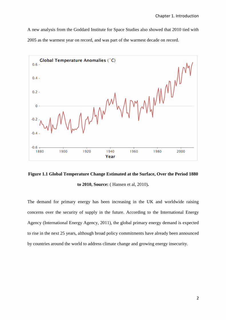
The ozone layer is depleting and global warming is taking place as we speak. There is now
enough evidence to suggest this, for example, some of the evidence can be found in data
gathered worldwide by the National Aeronautics and Space Administration’s (NASA)
Goddard Institute for Space Studies (GISS). The data which is presented in a paper by
Hansen et al (2010) shows the difference between surface temperature in a given month and
the average temperature for the same period during 1951 to 1980 as summarised in Figure
1.1.
Chapter 1. Introduction
2
A new analysis from the Goddard Institute for Space Studies also showed that 2010 tied with
2005 as the warmest year on record, and was part of the warmest decade on record.
Figure 1.1 Global Temperature Change Estimated at the Surface, Over the Period 1880
to 2010, Source: ( Hansen et al, 2010).
The demand for primary energy has been increasing in the UK and worldwide raising
concerns over the security of supply in the future. According to the International Energy
Agency (International Energy Agency, 2011), the global primary energy demand is expected
to rise in the next 25 years, although broad policy commitments have already been announced
by countries around the world to address climate change and growing energy insecurity.

Chapter 1. Introduction
3
Global installed power generation capacity and additional energy by technology in the current
policy scenario are illustrated in Figure 1.2. The graph shows that renewable energy sources
are expected to claim a greater proportion of installed power generation in the future and
global installed power generation capacity is expected to reach 9,000 GW by the year 2035
unless future policy changes are made.
Figure 1.2 Global Installed Power Generation Capacity and Additions by Technology,
Source: (International Energy Agency, 2011)
As a result global CO2 emissions are projected to rise at an even higher rate in future reaching
45 billion metric tonnes in 2030 as shown by the graph in Figure 1.3.

Chapter 1. Introduction
4
Figure 1.3 Actual and Predicted Carbon Dioxide Emissions by Region, 1990 – 2030,
Sources: (Energy Information & Administration, 2006).
As the world population grows more pressure is likely to be put on primary energy
production and consumption. China’s energy consumption for example has more than
doubled in the past two decades to cater for growth in various sectors the economy. This
growth is a direct result of the growth in population in that country (International Energy
Agency, 2006).
In 2006 the Energy Information & Administration (EIA), published in its “International
Energy Outlook” document a more comprehensive breakdown of global energy use and
carbon emissions by region, including energy use forecasts into the future up to the year 2030
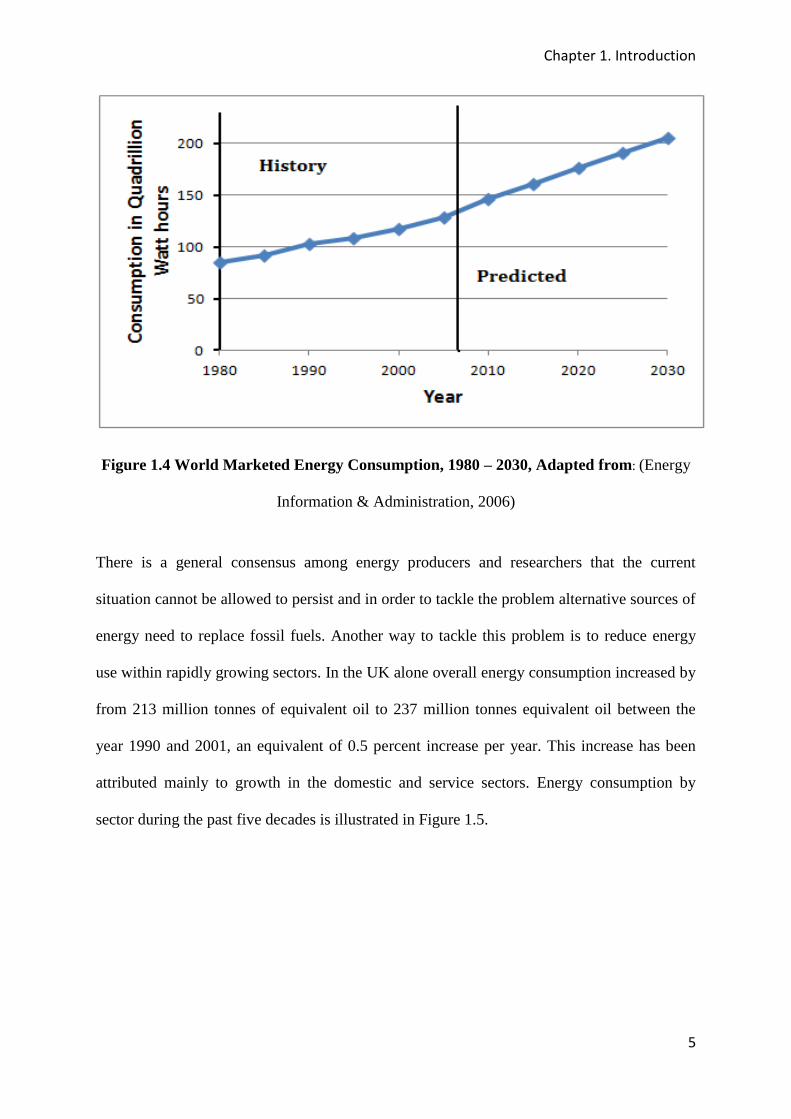
(Energy Information & Administration, 2006). World marketed energy consumption is
expected to reach 212 Quadrillion Giga Watt-hours by the year 2030 as shown in the graph in
Figure 1.4.
Chapter 1. Introduction
5
Figure 1.4 World Marketed Energy Consumption, 1980 – 2030, Adapted from: (Energy
Information & Administration, 2006)
There is a general consensus among energy producers and researchers that the current
situation cannot be allowed to persist and in order to tackle the problem alternative sources of
energy need to replace fossil fuels. Another way to tackle this problem is to reduce energy
use within rapidly growing sectors. In the UK alone overall energy consumption increased by
from 213 million tonnes of equivalent oil to 237 million tonnes equivalent oil between the
year 1990 and 2001, an equivalent of 0.5 percent increase per year. This increase has been
attributed mainly to growth in the domestic and service sectors. Energy consumption by
sector during the past five decades is illustrated in Figure 1.5.
Chapter 1. Introduction
6
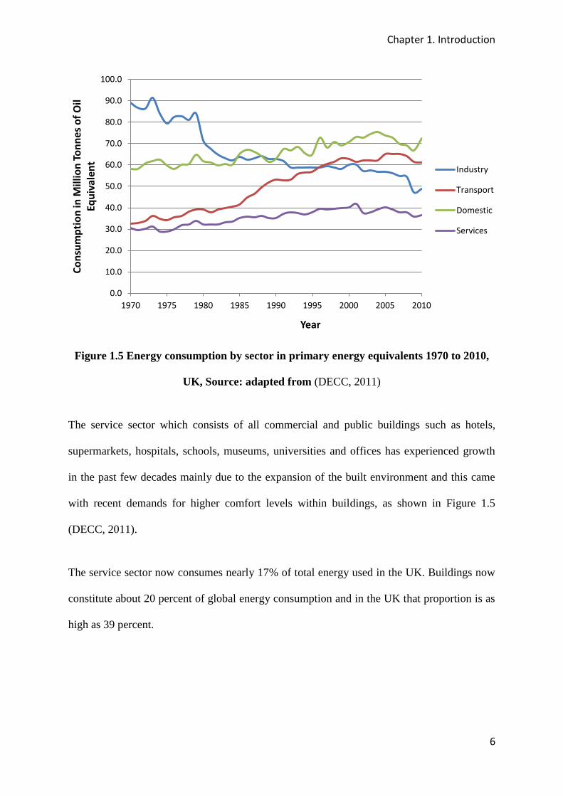
Figure 1.5 Energy consumption by sector in primary energy equivalents 1970 to 2010,
UK, Source: adapted from (DECC, 2011)
The service sector which consists of all commercial and public buildings such as hotels,
supermarkets, hospitals, schools, museums, universities and offices has experienced growth
in the past few decades mainly due to the expansion of the built environment and this came
with recent demands for higher comfort levels within buildings, as shown in Figure 1.5
(DECC, 2011).
The service sector now consumes nearly 17% of total energy used in the UK. Buildings now
constitute about 20 percent of global energy consumption and in the UK that proportion is as
high as 39 percent.
0.0
10.0
20.0
30.0
40.0
50.0
60.0
70.0
80.0
90.0
100.0
1970 1975 1980 1985 1990 1995 2000 2005 2010
Co
nsu
mp
tio
n in
Mil
lio
n T
on
ne
s o
f O
il
Eq
uiv
ale
nt
Year
Industry
Transport
Domestic
Services
Chapter 1. Introduction
7
In view of these facts, the European Parliament and Council approved in December 2002 a
directive on the energy performance of buildings (EPBD) (European Parliament and Council,
2003). The directive requires among other things the need to develop methodologies for
calculation of energy performance of buildings, set minimum requirements for energy
performance, apply the minimum requirements in new and existing buildings and develop
energy certification standards for buildings. The amount of energy consumed in buildings
depends significantly on the standards set for the indoor environment and the design and
operation of building systems. Setting criteria for the indoor environment involves setting
design standards for systems that control indoor temperature, relative humidity, ventilation
rates, lighting and acoustics. National and international standards and guidelines which
specify criteria for thermal comfort and indoor air quality have been developed. The
standards are cited as references throughout the body of this thesis.
The quality of the indoor environment affects health, productivity and comfort of the
occupants (Bjarne and Olesen, 2007; EN15251, 2006). Recent studies by Chiang et al
(Chiang and Lai, 2002) on the comprehensive indicator of indoor environment assessment
and others by Muhic et al (2004) have shown that the indoor environment has an effect on the
health comfort and productivity of occupants. Poor indoor environment quality can
negatively affect the profits of any organisation as the costs of absenteeism and low
productivity are most often higher than the costs of energy used in the building (Wong et al,
2007, CIBSE, 1986). On the other hand good indoor environment quality can improve overall
work performance by minimising the effects of building related illnesses and reducing
absenteeism (BRECSU, 2000).
Chapter 1. Introduction
8
Ratcliffe et al reviewed the effects of increasing energy efficiency on productivity in
commercial offices in the UK and acknowledged that although there is little incentive in
exceeding minimum standards set by building regulations, there are aspects of the indoor
environment such as the increasing use of daylighting and natural ventilation that show
significant positive correlations with productivity (Ratcliffe and Day, 2003). For example
there is a tendency among office occupants to have preferences for working areas near
windows.
In most cases occupants feeling uncomfortable tend to take action to improve the situation,
for example, by opening or closing windows, using fans to cool the space, adjusting the levels
of clothing or connecting an electric heater. Most of these rash actions are usually energy
intensive techniques that may increase both the bill and carbon emissions at the end of the
year. In the UK buildings are now required by law to display energy performance
certification (Building and Buildings - England and Wales, 2007).
However making energy performance declarations without declarations of the indoor
environment does not make sense since the criteria used for the indoor environment
significantly affects energy use. Methodologies for calculating energy performance of office
buildings have been developed in the UK. The challenge now is to develop IEQ assessment
methodologies that are comparable to energy use and which can be used to determine by how
much energy efficiency imperatives sacrifice human comfort. This thesis attempts to address
this specific problem area.

Chapter 1. Introduction
9
1.2 AI MS AND OBJECTIVES OF THE STUDY
The primary aim of this study is to provide a methodology for the development of a single
index based IEQAT (Indoor Environment Quality Assessment Tool) that can be used for
rating offices according to the quality of their indoor environment. The specific objectives of
this research are:
To develop a mathematical model for the IEQAT tool from extensive literature
review. This includes developing or adopting indices for thermal comfort, IAQ,
lighting and acoustic comfort with particular emphasis on variables that affect energy
use and occupant comfort;
To test the model by studying the responses of occupants of selected office buildings
in the United Kingdom. The responses which are collected via questionnaires will be
compared against model performance using physical measurements of parameters
such as air temperature, illuminance (lux), background noise levels (dBA), relative
humidity, carbon dioxide concentration (ppm), and air velocity as input;
To use the AHP to provide a provisional estimation of IEQ in selected offices; and
To use multiple regression modelling to determine a weighted ranking of contributing
parameters, based on the type of office building and hence develop single indices that
can be used to different rank different types of offices according to the quality of
their indoor environment.
Chapter 1. Introduction
10
The novelty and originality of the IEQAT is that it includes the following new aspects in IEQ
assessment:
It represents the first attempt at addressing the need to estimate IEQ in offices using
variables that have an impact on the energy performance of office buildings, hence it
allows tests on how much of occupant comfort is sacrificed by the choice of particular
energy efficiency imperatives to be made;
The new tool can also be used to determine IEQ of typical office spaces in the UK
context using calculated, measured, design and survey data. The tool can be used at
any stage of the building’s lifecycle i.e. it can be used during the design, construction
and operation of the building;
The methodology also includes new methods for estimating Acoustic and Lighting
Indices that reflect the opinion of the occupant. These indices combined with more
established thermal comfort and IAQ indices constitute the new index; and
The use of weightings derived from subjective evaluation of indoor environments to
develop a methodology for a computer tool for assessment of IEQ in office spaces in
the UK is new. It represents the need to explore new areas of research in an attempt to
develop a lasting solution to the problem of IEQ assessment using single index based
tools.

Chapter 1. Introduction
11
1.3 OUTLINE OF THE THESIS
A general outline of the thesis is illustrated in the flow chart in Figure 1.6.
Figure 1.6 Flowchart: The development of a methodology for assessment of IEQ in
office buildings.
Identify environmental input parameters for
Energy & IEQ assessment
Develop the IEQ Model from Literature
Use selected buildings to verify the IEQ Model
Determine weighting factors from study
Discuss the Methodology and Conclude
Chapter 1. Introduction
12
This chapter (Chapter 1) gives a brief background in energy use, building comfort and
global warming concerns in the UK and worldwide. The chapter also contains a brief
introduction to the PhD study, its aims and objectives including a brief outline of the thesis
and the novelty of the study.
Chapter 2 is a review of energy consumption in office buildings, energy use reduction
strategies including current legislation and IEQ analysis methodologies used for office
buildings in the UK. The chapter also presents various aspects of the indoor environment that
affect the occupant’s perception of IEQ. This includes a description of individual
components affecting IEQ and a review of previous studies in buildings. Current standards in
the operation of office buildings are also discussed in this chapter.
A chapter 3 presents the development of a Mathematical Model for calculating IEQ in office
spaces in the UK based on literature review. A formal mathematical specification of the
expression for IEQ acceptability is also highlighted in the model. Indices contributing
linearly to perceived IEQ and a step by step program on how to predict comfort in offices are
presented in this section. Recommended overall evaluation, classification and long term
evaluation of the indoor environment are presented based on the new methodology.
Chapter 4 describes the methodology used to determine the relative importance of each of
the proposed IEQ variables and methods used to evaluate the IEQ assessment tool developed
in Chapter 3. It begins by describing the study design, the buildings and occupant selection
procedures, the design of the questionnaire and a brief description of the equipment used to
collect measurements. The chapter concludes by looking at typical software used to collect
and analyse collected data.

Chapter 1. Introduction
13
Chapter 5 summarises the results of case studies used to test the IEQ model. Cases include a
natural, mixed mode and a mechanically ventilated office in urban settings. Comparisons
between calculated and surveyed comfort results are made in this chapter. IEQ results
calculated using the AHP are used as provisional IEQ model data throughout the Chapter.
Regression analysis of questionnaire data is used to determine relative weightings of each of
the five proposed IEQ parameters and hence new models are developed. The chapter also
highlights lessons that are learnt by studying each of the case buildings.
Chapter 6 presents the conclusions of the PhD study, the limitations of the IEQ
methodology, improvements to the methodology based on case study results and
recommendations for further work.
Chapter 2. Literature Review
14
2. Literature Review
2.1 ENERGY USE IN OFFICE BUILDINGS
2.1.1 Major End uses
Offices together with retail, hotels and restaurants are one of the largest consumers of energy
within the commercial/service sector (Wade and Ramsey, 2003). Researchers have been keen
to understand how much energy these buildings consume relative to others in the same sector.
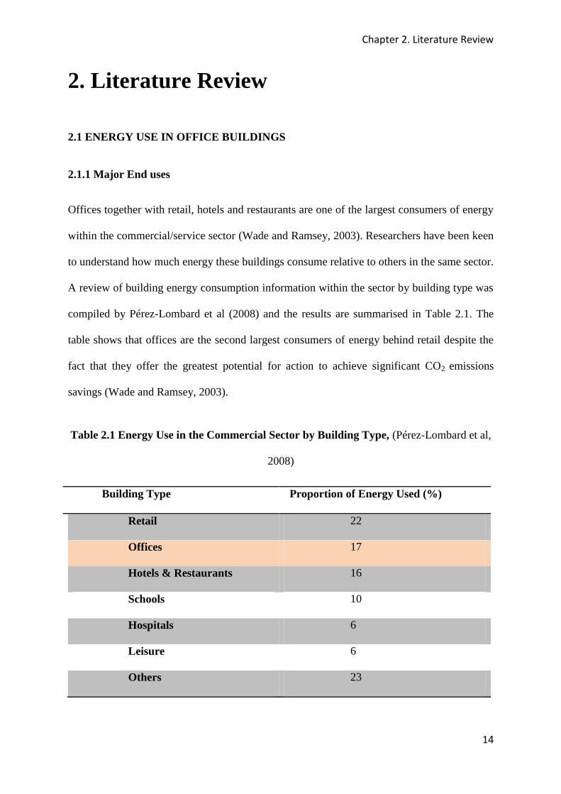
A review of building energy consumption information within the sector by building type was
compiled by Pérez-Lombard et al (2008) and the results are summarised in Table 2.1. The
table shows that offices are the second largest consumers of energy behind retail despite the
fact that they offer the greatest potential for action to achieve significant CO2 emissions
savings (Wade and Ramsey, 2003).
Table 2.1 Energy Use in the Commercial Sector by Building Type, (Pérez-Lombard et al,
2008)
Building Type Proportion of Energy Used (%)
Retail 22
Offices 17
Hotels & Restaurants 16
Schools 10
Hospitals 6
Leisure 6
Others 23
Chapter 2. Literature Review
15
Pérez-Lombard et al (2008) argued that energy supplied to office buildings is used in two
main areas, (1) building services and (2) equipment services. Building services uses include a
variety of applications such as HVAC, Domestic Hot Water (DHW), lighting and sanitary
facilities. HVAC systems constitute about 55 percent of energy used in offices in the UK and
most of this is channelled towards thermal comfort demands such as heating and cooling.
Heating and hot water needs of offices are largely catered for by burning fossil fuels such as
natural gas and petroleum products such as LPG.
In some cases electric immersion heating may be used in place of gas and oil boilers
(BRECSU, 2000, Pérez-Lombard et al, 2008). Electric heating tends to contribute more
carbon emissions as most of the electricity supplied to office buildings comes from power
stations. Cooling uses significant amounts of electricity although it uses less compared to the
pumps and fans which distribute the heat or coolant to various parts of the building. Lighting
is yet another high end user of electricity despite efforts being made to increase the
contribution of daylighting in new office designs (BRECSU, 2000).
Equipment uses include computers, printers, food preparation equipment, etc and these are
mainly powered by grid electricity (Picklum et al, 1999). Electricity is also used in other
areas including parking lots, lifts and security systems and the amount used increases with the
complexity of the building as a whole. Prestige offices with a large range of services tend to
consume more compared to simpler ones. Table 2.2 is a summary of energy use in office
buildings by type of end use as prepared by Scras et al (2000). The table shows that by the
year 2000 space heating and lighting consumed most of the energy in the UK.

Chapter 2. Literature Review
16
Table 2.2 Energy Use in Offices by End Use in the UK (Scras, 2000)
Building Services Uses Amount of fuel
used (Peta Joules)
Equipment Uses Amount of fuel
used (Peta
Joules)
Heating
Hot water
Cooling
Fans/Pumps/Controls
Lighting
Process
51
5
11
2
16
3
IT
Catering,
Other electricity –
lifts, exterior lighting;
& special equipment
rooms, etc.
8
6
2
Another breakdown in energy use in offices was compiled by Perez-Lombard in 2008 and the
results are summarised in Table 2.3. It is important to note that HVAC systems and lighting
consume a total of more than 70 percent of energy used in the buildings therefore targeting
these areas is an important step towards reducing energy use in offices.
Table 2.3 Proportion of Energy Consumption in Offices by End Use (Pérez-Lombard et
al, 2008)
Energy End Uses Proportion of Usage
HVAC 55
Lighting 17
Equipment (Appliances) 5
DHW 10
Food Preparation 5
Refrigeration 5
Others 4

Chapter 2. Literature Review
17
According to research carried out by EIA and DTI (Energy Information & Administration,
2006) offices are responsible for CO2 emissions of well over 2.2 million tonnes per year
(D.T.I., 2002). Results of a research funded by DEFRA in 1998 provided a breakdown of
energy use and CO2 emissions by type of occupier, end use and fuel type (Pout et al, 2000).
Data for commercial offices was extracted and it is presented in Table 2.4.
Table 2.4 Energy consumption and CO2 emissions in UK Commercial Offices: source –
Wade and Ramsey (2003), Research carried out by Pout et al* (2000).
Fossil Fuels (PJ) Electricity (PJ) CO2 (kT)
Heating 46 5 3680
Hot Water 5 0 469
Catering 3 3 370
Light - 16 2238
Cooling - 11 1319
Small Power - 2 250
IT - 12 1031
Other - 2 184
Process - 3 7
Unknown - 0.3 121
Total 54 56 9669
* CO2 data includes emissions from power stations

Chapter 2. Literature Review
18
The amount of energy used in an office building depends on the type, size and operation of
that building. In other words the amount of energy used in an office building depends on the
design standards of the building and its services. Offices where a high level of performance
is expected are more likely to consume more energy than those with lower levels of
expectation. Whether the building is mechanical or naturally ventilated (presence of air
conditioning) has a large bearing on the amount of energy used since the use of air-
conditioning adds considerably to the energy demand of office buildings (BRECSU, 2000).
The proportion of open plan space also has an effect on the amount of energy used as these
tend to use more energy particularly for lighting (BRECSU, 2000). For this reason The
Energy Efficiency Best Practice Programme has studied typical and good practice energy
consumption in four types of offices and the results are summarised in Table 2.5. The
exercise is aimed at encouraging positive management action in order to improve the energy
and environmental performance of offices. Good Practice is described in the Energy
Consumption Guide 19 (BRECSU, 2000) as a situation in “which significantly lower energy
consumption has been achieved using widely available and well-proven energy-efficient
features and management practices”.
Typical Practice is described as energy consumption patterns, which are consistent with
median values of data collected in the mid-1990s for the Department of the Environment,
Transport and the Regions (DETR) from a broad range of occupied office buildings”. Table
2.5 gives benchmarks against which one can compare the performance of their own office
building and highlights that typical high performing offices tend to use more energy that low
performing counterparts. For example a typical prestige office consumes 2.8 times more
energy per unit of floor area than a typical naturally ventilated cellular building and “Typical”

Chapter 2. Literature Review
19
offices in general use 60% to 90% more energy than “good practice” offices (BRECSU,
2000).
Table 2.5 Typical and Good Practice Energy Consumption in Offices in the UK (Wade
and Ramsey, 2003)
kWh / m2 of treated floor area
Naturally ventilated cellular
Naturally ventilated open plan
A/C, standard A/C prestige
Good
Practice
Typical Good
Practice
Typical Good
Practice
Typica
l
Good
Practice
Typical
Heating/Hot
Water
79 151 79 151 97 178 107 201
Cooling 0 0 1 2 14 31 21 41
Fans/Pumps, etc 2 6 4 8 30 60 36 67
Humidification 0 0 0 0 8 18 12 23
Lighting 14 23 22 38 27 54 29 60
Equipment 12 18 20 27 23 31 23 32
Catering 2 3 3 5 5 6 20 24
Other 3 4 4 5 7 8 13 15
Computer Room 0 0 0 0 14 18 87 105
Total 112 205 133 236 225 404 348 568
Chapter 2. Literature Review
20
The amount of energy used in buildings has been rising in the past few years in the UK and
the rise has been attributed to three reasons (BRECSU, 2000). First, there has been a
significant growth in the information technology sector and a rise in the use of air
conditioning systems to improve comfort in recent years. The demand for electricity for
cooling has been increasing and it is expected to rise significantly in the near future since
only a small proportion of office space is currently air conditioned. Over half of the offices
that were built in the 1990s had air conditioning systems installed and during the last decade
the number of chiller units sold to the UK market has more than tripled. Almost 45% of the
units were installed in commercial offices reflecting the need for higher performing offices in
that area (Giles, 2002).
Upgrading new and existing offices will mean the use of air conditioning technologies to
ensure appropriate IEQ will be a common feature in the developed world in the next decades
(Adnot, 2003). The electrical air conditioning load is subject to sharp peaks in demand for
power during certain times of the day and this causes strain to the utility suppliers. This
coupled with the rise in the amount of office equipment used will likely influence the future
source of supply of electricity. Office equipment now accounts for about 5 percent of energy
used in office buildings as the use of computers, printers, copiers, vending machines and
communication equipment such as servers continue to increase (Pérez-Lombard et al, 2008).
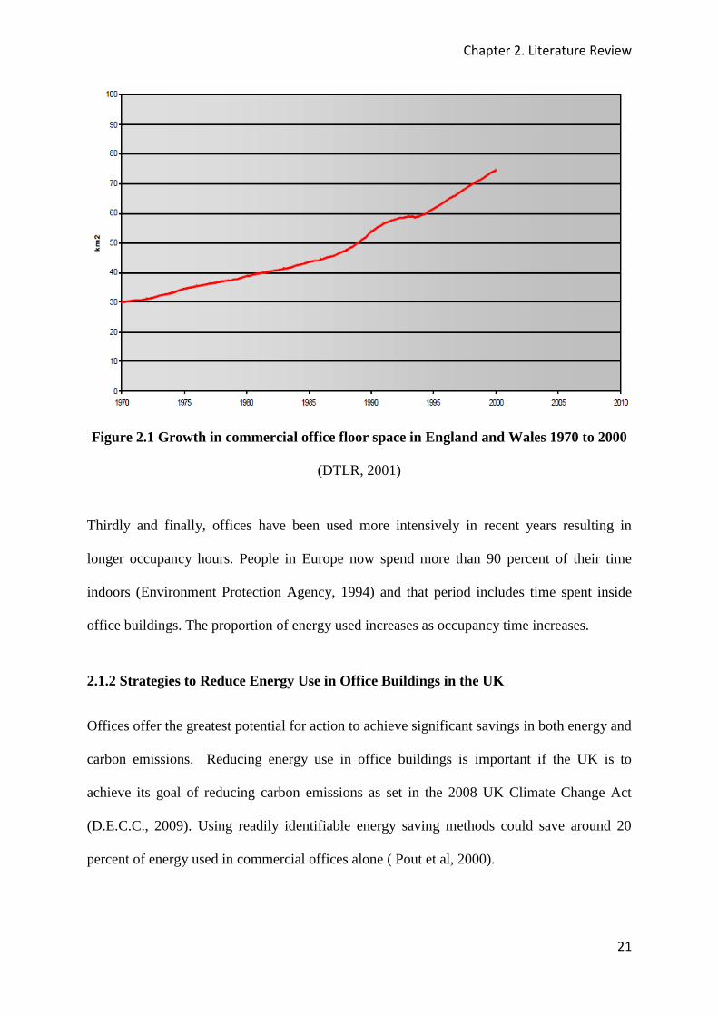
Secondly, there has been growth in the number of new buildings erected in the UK. The new
build rates within the service sector are typically around 2% and forecasts show that this rate
is set to continue increasing (Pérez-Lombard et al, 2008). Figure 2.1 demonstrates a rapid
growth in commercial office floor space since the early 1970s in England and Wales. From
1980 to 2000 the total office floor space almost doubled.
Chapter 2. Literature Review
21
Figure 2.1 Growth in commercial office floor space in England and Wales 1970 to 2000
(DTLR, 2001)
Thirdly and finally, offices have been used more intensively in recent years resulting in
longer occupancy hours. People in Europe now spend more than 90 percent of their time
indoors (Environment Protection Agency, 1994) and that period includes time spent inside
office buildings. The proportion of energy used increases as occupancy time increases.
2.1.2 Strategies to Reduce Energy Use in Office Buildings in the UK
Offices offer the greatest potential for action to achieve significant savings in both energy and
carbon emissions. Reducing energy use in office buildings is important if the UK is to
achieve its goal of reducing carbon emissions as set in the 2008 UK Climate Change Act
(D.E.C.C., 2009). Using readily identifiable energy saving methods could save around 20
percent of energy used in commercial offices alone ( Pout et al, 2000).
Chapter 2. Literature Review
22
Every effort needs to be made to implement energy saving measures in new and existing
office buildings. For new buildings some of the measures include the use of energy efficient
office designs such as those which maximise the use of good building fabric and form to
control the internal environment (Carbon Trust, 2000). For example target U values of
0.15W/m2.K for walls result in buildings that have very good thermal properties (higher end
of the spectrum). Lower U values for windows, ceiling, doors, and floors also contribute to
reduced energy use in buildings; so does the minimisation of thermal bridges where possible
and the improvements in building air tightness.
Other measures that can be applied to new buildings include the use of better architectures
such as the use of atria for natural daylighting, passive cooling strategies, advanced glazing
and reduced building depths (Carbon Trust, 2000, BRECSU, 2000). Designs which facilitate
effective use and control of building services such as the BMS are also encouraged. Another
way of improve energy performance of new office buildings is to target HVAC systems by
designing passive ventilation systems (stack ventilation).
For existing buildings, management of the building thermal load, general energy efficiency,
efficient operation of energy systems and the use of natural energy are of paramount
importance. Energy efficiency in the building service system includes improvements in
HVAC systems, lighting systems, hot water supplies, office equipment, elevators, etc.
Monitoring of occupancy hours, the use of operation and management systems, improved
maintenance services and reduced use of unoccupied spaces can help save energy (Picklum et
al, 1999).
Chapter 2. Literature Review
23
Sustainable technologies such as Combined Heat and Power (CHP), heat pumps, condensing
boilers, wind turbines and solar products are now finding wider applications in commercial
buildings and they help significantly reduce carbon emissions. They can be use in both new
and existing buildings where opportunities exist. Improved controls of optimisers that help
avoid overheating, cooling and unnecessary lighting (occupancy sensors) are becoming
increasingly important. The use of energy efficient lighting such as fluorescent lamps and
lighting timers is strongly encouraged. Changing consumer behaviour is also critical if the
above measures are to be successful (Pérez-Lombard et al, 2008, Picklum et al, 1999).
Finally the Energy Review (PIU, 2002) highlights the need to improve energy efficiency in
buildings and recommends “action to deliver a phased transition to low energy commercial
buildings through development of the Building Regulations”. Legislation can play an
important role in driving change towards a low carbon lifestyle. The UK government has put
in place legally binding, long term frameworks based on the Kyoto Protocol (UNFCC, 1998).
This framework has been put forward in the form of regulations, directives, taxation and
incentives.
The Energy Efficiency Commitment (EEC) (OfGEM, 2007) was set to encourage electricity
and gas suppliers to make energy savings by working in partnership with project partners
such as social housing providers, charities and retailers. The EEC phase 1 started in 2002 and
EEC 2 ran from 2005 to 2008, while EEC 3 which began in April 2008 is expected save 293
million lifetime tonnes of carbon. Beyond the Kyoto protocol Part L building regulations
(Department for Communities and Local Government, 2006) came into effect in 2006
(revised in 2010) to help enforce energy reduction commitments and some of the
requirements for both new and existing non domestic buildings are found in Part L1A, L1B,
L2A and L2B. The Energy Performance of Buildings Directive (EPBD) (European

Chapter 2. Literature Review
24
Parliament and Council, 2003) which was issued by the European parliament in 2002 is
embodied in the UK Buildings regulations (Department for Communities and Local
Government, 2006).
The directive requires among other things that member countries develop methodologies for
the calculation of integrated energy performance of buildings, set minimum standards for
energy performance of new buildings, apply requirements to existing buildings and develop
certification systems for energy use in all buildings (European Parliament and Council, 2003,
Department for Communities and Local Government, 2006). It also suggests that cost
effective measures should be included where major renovations of buildings are carried out in
order to improve energy efficiency (European Parliament and Council, 2003). The directive
provides a general framework for calculation of energy performance of buildings based on
the following:
Thermal characteristics of the building, heating and hot water installations;
Air conditioning;
Ventilation;
Built in Lighting;
Building position, orientation, effect of outdoor conditions and passive solar systems;
Natural ventilation; and
Indoor Environment Quality (IEQ).
In this thesis more focus is on the IEQ aspects of commercial office buildings.
Chapter 2. Literature Review
25
2.2 THE INDOOR ENVIRONMENT
2.2.1. Introduction
Providing and maintaining the required indoor environment quality is an energy demanding
exercise that requires designers, owners and energy users of buildings to make a balance
between energy saving imperatives and providing comfort (Bjarne and Olesen, 2007). The
quality of the indoor environment is described in the EN15251 standard (EN15251, 2006) as
depending on the design and operation of building systems that control temperature,
humidity, ventilation rates and illuminance. It also depends on the interaction between the
occupant and the building envelope and its acceptability depends on how occupants accept
the thermal environment, indoor air quality, acoustics and lighting comfort. These aspects
and many other little understood factors such as vibrations, workplace design,
electromagnetic effects, etc constitute what is perceived as IEQ by occupants and they will be
highlighted in the subsequent sections in this Chapter. Some researchers have found that
factors such as individual physiological state, health, social relations, financial state, state of
adaptation to the climate and other person specific factors contribute to subjectively
perceived IEQ (ASHRAE, 1993).
2.2.2 Overview of IEQ Assessment in Office Buildings
The way IEQ is perceived is viewed by many scholars (Jokl, 2003, Bjarne and Olesen, 2007)
as a complex phenomenon that requires some knowledge of how the human body system
functions. Jokl (2003) highlighted the different types of stimuli that affect our perception of
the indoor microclimate as shown in Figure 2.2. The diagram also highlights the importance
of four main aspects of the indoor environment namely, thermal, aural, acoustic and visual
environment.

Chapter 2. Literature Review
26
Figure 2.2 Main constituents of stimulus in indoor microclimate (Jokl, 2003)
Several attempts have been made by researchers to develop methodologies for assessment of
IEQ in offices and similar environments globally. One such attempt was carried out by
Chiang et al (2000) in aged care buildings in Taiwan. The researchers graded IEQ parameters
such as carbon dioxide and carbon monoxide concentrations, dust particles, air velocity, air
temperature, mean radiant temperature, relative humidity, noise level and illuminance into
categories based on comparisons with recommended (health related) values in those
buildings. The results of the model (field measurements) clearly showed close congruence
with subjective assessments. The study highlighted the fact that comprehensive assessments
of various integrated factors of the physical environment are still developing and in this case
the point scoring system was based less on occupant perception the indoor environment. It
should be expected that more credibility should be given to systems that reflect the opinions
of the occupants (Lai et al, 2009).
Chapter 2. Literature Review
27
Mui and Chan (2005) developed the so called Building Environmental Performance Model
(BEPM) which compared building energy use with satisfaction with the indoor environment.
The BEPM tool incorporated the adaptive comfort temperature control approach and a CO2
demand control module which made it possible for the building management system to
maintain thermal satisfaction whilst maintaining optimum energy consumption. However two
other important parameters namely lighting acceptance and acoustic comfort were not
incorporated into the system. The adaptive thermal comfort model also made the BEPM only
suitable for naturally ventilated office buildings.
Most current standards cover separate aspects of the indoor environment, for example the
EN15251 (2006) covers thermal comfort, Air Quality, Acoustics and lighting. The standards
also show a strong focus on the development of recommendations for acceptable indoor
environments making allowances for national differences in the requirements as well as for
designing buildings for different quality levels (Olesen, 2004). However, satisfaction or lack
of with each aspect is considered separately suggesting that there is a general lack of
evidence that interactions between them exist, although it is common knowledge that all of
the aspects play a part in the way occupants rate the indoor environment.
A study carried out by Toftum and King (2002) on the way humans respond to combined
indoor environment exposures concluded that there was little evidence of significant
interactions between different aspects of the indoor environment suggesting that these aspects
acted exclusively on occupants. Only the effects of air temperature and relative humidity
were found to be linked to perceived air quality suggesting that the combined effects of the
parameters could be additive to some extent. How the parameters combine to influence IEQ
has proved to be the most elusive part of the conundrum.

Chapter 2. Literature Review
28
Bjarne and Olesen (2007) has attributed this to lack of knowledge of how various aspects can
be added together to form a single representative index since their relative weightings are not
known. Lai et al (2009) examined the quality of the indoor environment from the prospect of
an occupant’s acceptance in four aspects: thermal comfort, indoor air quality, noise level and
illumination level. This provided some basis on which models that predict the quality of the
indoor environment given a set of conditions could be developed.
Lai used the operative temperature as a basis for thermal acceptance of the indoor
environment and gave occupants the freedom to adjust their clothing based the prevailing
conditions. This study follows an earlier study conducted by Wong et al (2007) in which a
logistic model was used to determine the overall acceptance of the IEQ based on weighting
factors derived from subjective evaluations. This approach is more practical in naturally
ventilated office environments and improvements need to be made before it can be accepted
in a variety of environments.
Perhaps the most compelling study was carried out by Chiang and Lai (2002) who developed
a comprehensive indicator of the indoor environment in office buildings using a consultative
process involving building services experts in Taiwan. The researchers used the Analytical
Hierarchy Process to derive weightings of each of the four main contributors to overall IEQ.
This process will be described further in Chapter 3, Section 3.35.
Chapter 2. Literature Review
29
2.2.3 Current IEQ Assessment Tools
The building sector has witnessed several criteria based tools for the assessment of
environmental performance (including IEQ) of office buildings. Most of the tools are
considered as comprehensive since they assess a variety of parameters such as energy use,
indoor environment, water usage, materials usage, recycling, etc. The analysis tools have
varying levels of accuracy hence they have been applied at different stages of design and
operation of office buildings. Some of the most recognised tools include the BUS occupant
survey developed by the Usable Buildings Trust (Boarders, 1981). This tool can be used for
quickly assessing building IEQ performance (among other aspects of building performance)
primarily from the feedback of occupants hence it is more applicable during post occupancy
evaluation of office buildings.
The most predominantly used tool is the BREEAM tool which was developed by the
Building Research Establishment (BRE, 1990). This voluntary assessment tool is used for
environmental assessment of building performance using recognised measures of
performance which are set against established benchmarks. The tool has a health and well
being aspect which is of interest to this research. Its French counterpart, the “Haute Qualité
Environnementale” (High Quality Environment, HQE) was developed by the Paris based
Association for High Quality Environment (ASSOHQE) (2002) and contains advice on how
to create pleasant indoor environments and tips on how to manage the impacts of the outdoor
environment on conditions inside buildings. Both the BRE and the HQE have made efforts to
develop a Europe wide building environmental assessment methodology and in 2009 they
signed a memorandum of understanding to work together towards this goal.
Chapter 2. Literature Review
30
Other international tools include the Green Star Scheme developed by the Green Building
Council of Australia (GBCAUS, 2003) to assess the environmental performance of buildings
in specific sectors, e.g. in offices, retails, education, and at a distinct phases of the
development cycle. The tool also assesses IEQ among other aspects of building performance
and like most assessment tools the point scoring criteria aspects of the indoor environment
could be improved to reflect the view of the occupant. The LEED Post Occupancy Evaluation
Methodology for Offices (POEM-O) is one of the tools and it was developed by the U.S.
Green Building Council (USGBC, 1998) as part of a whole-building approach to
sustainability. Its main disadvantage is that it can only be used at post occupancy stage of a
building’s life cycle.
The Australian NABERS rating system (Nabers, 2010) is a comprehensive performance-
based rating system for existing buildings which also assesses IEQ. It is used as a voluntary
tool which is used mainly for assessment of homes, offices, hotels, retail, transport, hospitals
and offices across Australia and New Zealand. However, this rating system ignores the
importance of lighting to occupant perception of IEQ in office buildings. The method can
only be used for existing buildings hence it cannot be used as a design tool. Finally the
Sustainable Building Consortium of Japan developed the CASBEE assessment tools (IBEC,
2008) for use in a wide range of buildings (offices, schools, apartments, etc.).
The main advantage of most tools is that each of them is developed to assess building
performance at a specific stage of its lifecycle, i.e. tools have been developed for pre-design,
new construction, existing buildings and renovations. The major disadvantages of the indoor
environment assessment components is that it is difficult to compare the scoring of indoor
environmental parameters to the health and well being of occupants. This has prompted a call
for novel approaches, other than questionnaires, that reflect the perceptions of the occupant.

Chapter 2. Literature Review
31
New tools need to generate predictions that correlate well with subjective assessments.
Another common feature in most tools is that they treat IEQ indices such thermal comfort,
IAQ, acoustics and lighting as separate entities hence it is difficult to use them for
comparison with energy use.
2.3 THE THERMAL ENVIRONMENT
2.3.1 Overview of Thermal Comfort Assessment in Office Buildings
One of the primary objectives of buildings is to provide a comfortable thermal environment
for occupants. The creation of comfortable thermal conditions is an energy demanding
exercise that requires designers and building users to strike a balance between energy saving
and occupant comfort (Bjarne and Olesen, 2007). Fanger (1973) identified six main factors
affecting perceived thermal comfort as air temperature, mean radiant temperature, air
velocity, relative humidity, clothing insulation and activity levels. How these factors combine
to influence thermal comfort (ISO 7730, 2005) will be explained in Chapter 3.
Thermal comfort is defined in the ASHRAE Standard 55 (ASHRAE, 2005) and in ISO 7726
(1988) as “that condition of mind that expresses satisfaction with the thermal environment
and is assessed by subjective evaluation” (ASHRAE, 2005). That state of mind is a complex
link between the physiology and psychology of an individual; between the building occupant
and the heating ventilation and air conditioning system (HVAC) or the building’s architecture
(ASHRAE, 1993; Wolkoff, 2003; Humphreys, 2007). This complex link is illustrated in the
Cylindrical Model of Thermal Interaction of Human Body and the Environment shown in
Figure 2.3.

Chapter 2. Literature Review
32
The Cylindrical Model is one of the models that have been successfully used in practice and
it shows that the regulation of human bodily functions and activities depends on the
generation, storage and dissipation of heat (ASHRAE, 1993, CIBSE, 1986). Principles of
thermoregulation are widely found in various texts (Ganong, 2003; Hensen, 1991) and they
will not be described further in this thesis. The cylindrical model, which is incorporated in
many thermal comfort standards and thermal comfort assessment systems, is explained below
(ISO-7730, 2005; ASHRAE, 2005).
Figure 2.3 The Cylindrical Model of Thermal Interaction of Human Body and the
Environment, Adapted from ASHRAE, Page 8.1(1993).
Research has shown that individuals within buildings sense skin temperature rather than air
temperature (CIBSE, 1986, Olesen and Parsons, 2002) therefore it is the skin temperatures

Chapter 2. Literature Review
33
and other signals received by the receptor organs from the surrounding environment that
constitute what is perceived as hot, cold, warm, cool, etc. The perceptual responses are of
greatest significance in determining personal thermal comfort and they are measured by
subjective evaluation on a widely accepted 7- point ASHRAE thermal sensation scale
(Fanger, 2002; ASHRAE, 2005).
The ASHRAE thermal sensation scale was developed by Rohles and Nevins in 1971 and
modified by Rohles in 1973 (Olesen and Parsons, 2002). Their studies on college students led
to the discovery of correlations between perceived comfort and temperature, humidity and
exposure times among other variables. The asymmetrical scale has two extreme ends of
comfort i.e. the hot and the cold ends (a state of permissible thermal conditions called
discomfort and a state of non-permissible conditions generally referred to as unacceptable)
with the neutral (a state of balance in heat production and heat loss is often judged by people
as optimal) as the most ideal situation. Table 2.6 shows the seven point ASHRAE thermal
sensation scale.
Table 2.6 Seven Point ASHRAE Thermal Sensation Scale (CIBSE, 1986)
Chapter 2. Literature Review
34
Thermal comfort evaluation indices are the most researched of all IEQ indices and a number
of thermal comfort equations as proposed in some widely used design guides and standards.
Over the past 60 years much research effort has been devoted to their development and only a
few will be considered here. More information on thermal comfort indices can be found in
the CIBSE and ASHRAE handbooks (CIBSE, 1986, ASHRAE, 1984) or in Fanger’s
textbook on thermal comfort (Fanger, 1973). One of the first indices to be developed was the
Effective Temperature Scale (ET) which was developed in 1923 by Houghten et al and was
revised in 1941 by Houghten and Ferderber (1941). In this index researchers proposed that (i)
the temperature of the air, (ii) its moisture content, (iii) air movement and (iv) the radiation
transfer between the body and surrounding surfaces are the four main parameters affecting
thermal comfort. In their research the authors acknowledged that the most important
parameter affecting thermal comfort was dry bulb temperature.
The ET scale has however been criticised in various texts because it underestimated the
effects of humidity at high temperatures, and overestimated the effects of humidity at lower
temperatures (CIBSE, 1982). The Standard Operative Temperature is another early index
which has been applied in both the veterinary and human sciences fields. The index which
was developed by Gagge in 1940 takes into account the combined effects air temperature,
radiant temperature and air movement in calculating Thermal comfort (Gagge, 1940). The
scale was modified by Nishi and Gagge in 1941 (Gagge, 1970) to include the effects of
humidity. The scale was only applicable in moderate air velocity situations and only when the
values of operative temperatures were close to air and mean radiant temperatures. Other
models such as the two-node model of human thermoregulation were developed by Gagge
and Nevins in 1975 (Nevins et al, 1975).
Chapter 2. Literature Review
35
More recently several methods for evaluating thermal comfort in indoor environments have
been put forward by the International Standards Organisation (ISO), ASHRAE and CIBSE.
They include the assessment of the influence of the thermal environment on occupants using
subjective judgement scales (EN10551, 2010), the application of standards to people with
special requirements (BSI-EN, 2005), the evaluation of thermal environments in vehicles
(EN14505, 2009), the methods for assessment of human responses to contact with surfaces at
moderate temperatures (ISO13732-1, 2006), the analytical determination of thermal comfort
using Predicted Mean Vote (PMV) and Predicted Percentage Dissatisfied (PPD) indices and
local thermal comfort criteria such as Draught rating, discomfort due to vertical air
temperature difference and radiant temperature asymmetry (EN-ISO7730, 2005). The later
models which are mostly applicable in office buildings are explained further in Chapter 3,
section 3.3.1.
Even more recently thermal environment assessments involving advanced physiological
measurements, computer models, mathematical simulations (differential equations) and
thermal manikins have been developed by researchers. Studies involving heated, breathing
and sweating manikins have been done by Havenith et al (2008) while Fiala et al (2008),
introduced a multi-node model of human physiology to predict dynamic thermal comfort
responses to the indoor environment. Fiala et al (2008) measured temperatures of different
parts of the body at varying temperatures and found good correlations between core body
temperature and thermal sensation.
Chapter 2. Literature Review
36
Earlier Zhang (2004) and his colleagues had performed experiments on occupants under non
uniform transient conditions and developed predictive models of local, overall thermal
sensation and general comfort (Zhang et al, 2004). The models predicted thermal comfort
with reasonable success. However PMV and adaptive models still remain the models of
choice in office buildings (Parsons, 2008).
The PMV and PPD models have been tested extensively in air conditioned buildings
worldwide. In many thermal comfort studies, researchers have investigated the relationship
between actual thermal sensations (observed) to those predicted by the PMV model. Charles
(2003) carried out assessments of office buildings located in the North American region
(COPE Projects – Canada) using the PMV model and found that the model was a better
predictor of thermal comfort in air-conditioned buildings than in naturally ventilated ones.
The author attributed this to the influence of adaptation opportunities and outdoor
temperatures. The researchers also found differences between predicted and observed PMV
values but that the discrepancy between PMV and actual mean vote increased for heavier
clothing and higher activity levels (Charles, 2003).
A field study carried out by Melikov et al (2005) in 10 offices equipped with displacement
ventilation systems indicated that there was an overlap in those occupants dissatisfied with
uncomfortable room temperature, draught and vertical temperature difference. For example
the study found that about 49% of the occupants expressed dissatisfaction with air
temperature (cold) and 24% expressed dissatisfaction with draught and vertical temperature
difference (Melikov et al, 2005). Although the study did not indicate how many of the
occupants expressed dissatisfaction with both sets of discomfort factors it highlights the need
to approach discomfort estimations cautiously and precisely, that discomfort factors need to
be treated as risk factors if they are to be added together.

Chapter 2. Literature Review
37
Different models have been developed for office environments that are naturally ventilated
and the most notable include those developed by Humphreys (1994) and earlier models by
Auliciems (1981). The latter model is discussed further in Chapter 3, section 3.3.1. Studies
carried by Fanger and Toftum (2002) on office occupants in warm climates highlighted that
occupants in those climates may sense warmth as being less severe than the PMV model
predicts. They attributed this to low expectations of building thermal performance based on
conditions outside the building. As a consequence the researchers developed a new extension
of the PMV model based on the effects of adaptation to naturally ventilated buildings.
Observed thermal sensation votes on the 7 point ASHRAE scale agreed well with new
extensions of the PMV model in three continents.
2.4 INDOOR AIR QUALITY
2.4.1 Air Quality problems in buildings
Air quality is perceived by humans using the combination of the olfactory sense which is
situated in the nasal cavity and the general chemical sense which is situated all over the
mucous membranes in the nose, eyes and throat (Berglund et al, 1982). The olfactory sense is
sensitive to a very large number of odours in the air while the general chemical sense is also
sensitive to a large number of air pollutants, (hundreds of thousands of chemicals) (Seppänen
et al, 1999; NOHS, 2003).
Literature suggests that a combination of these senses determines whether the air is fresh,
stuffy, irritating, pleasant, dry, etc (Commission for European Communities, 1991, European
Collaborative Action, 1992). The science of perception is beyond the scope of this thesis and
it can be found in various texts, notably in “The Fundamentals of Human Sensation” by
Roberts (2002).
Chapter 2. Literature Review
38
Jokl (2003) highlighted that perceived air quality is dependent on the temperature of the air,
relative humidity, the concentration of chemical and biological elements in air, static
electricity and the number of ionic substances in the air. The impact of each of these factors
depends on the magnitude of the stimuli and perception of IAQ is solely based on our sensory
evaluation of odour microclimate. Acute and chronic illnesses emanating from poor indoor
air quality (IAQ) are very common in the UK (Ganong, 2003).
Studies have shown that buildings are the main route to exposure to air pollutants (Hensen,
1991) because as explained earlier in the thesis, most people in Europe spend most of their
time indoors. Research carried out by scientists in the USA suggest that the quality of indoor
air in these buildings can have major effects on health, comfort and productivity of occupants
(ASHRAE, 2007b). Some studies have highlighted the negative effects of poor IAQ on health
and productivity of offices occupants and school children (International Energy Agency,
2006; Berglund et al, 1982; Seppänen et al, 1999; Ratcliffe and Day, 2003).
If good indoor air quality is to be maintained, it is important to identify all important
parameters affecting it, develop appropriate assessment criteria and present appropriate
technologies that can be used to minimise its adverse impact on human occupants. The
scientific committee of the World Health Organisation have warned that pollutants that exist
at lower concentrations e.g. Volatile Organic Compounds (parts per million, etc) are still
potent enough to cause health problems (WHO, 1984). Pollutant mixtures have been found to
have complicated links to negative health outcomes, for example; their combined effects may
be or may not be synergistic, addictive, antagonistic or independent.

Chapter 2. Literature Review
39
At present it is difficult to predict the impact of any one or combination of chemicals which
usually exist in large numbers at any one particular time as suggested in studies by Hui et al
(2008). It is fairly good to assume control of pollution sources by using local ventilation
systems, isolation of pollutants, removal of sources of pollution, replacement of faulty
equipment, or controlling dominant sources of pollutants as explained earlier. Some
researchers suggest (ASHRAE, 1993; European Collaborative Action, 1992; Environment
Protection Agency, 1994; Fang et al, 2005; ASHRAE, 1985) identification of the dominant
source then calculating the required ventilation rate to remove it as an effective method for
minimising air pollution.
Controlling the dominant source is likely to remove all other air pollutants, therefore it is
perfect to assume that other chemicals will be sufficiently diluted using this approach. Indoor
air quality also varies with time in spaces due to occupant activity, outdoor conditions,
building operation and the types of building materials (low or high polluting). Human beings
produce bio effluents such as the carbon dioxide gas which pollutes indoor air. Carbon
dioxide levels in office buildings can thus be used as an indicator of air pollution.
Studies by Toftum and Fanger (2002) show that in many buildings human requirements of
the indoor environment vary throughout the day, with vulnerable individuals being more
sensitive to changes while healthy adults are less sensitive. The use of ventilation to improve
air quality is an established practice (Olesen and Parsons, 2002) although in most cases
ventilation is only set to meet the metabolic requirements of occupants and dilute their bio
effluents.

Chapter 2. Literature Review
40
Health aspects of IAQ are discussed by the WHO, UN and in the ECA’s 10th and 11th
publications (Effects of IAQ pollution on human health) (European Collaborative Action,
1992, Commission for European Communities, 1991). The above sources suggest that in
order to minimise the health effects of poor IAQ it is essential to establish a guide that
includes an extensive list of known indoor air pollutants of various origins with maximum
permissible limits & expose times associated with negative health outcomes. Legally binding
IAQ guidelines exist only for industrial spaces but not for non-industrial premises such as
offices where concentrations are usually very low (Fang et al, 2004, Daisey, 2003).
2.4.2 Overview of IAQ Assessment in Office Buildings
A number of approaches exist for the evaluation of building ventilation and indoor air quality
(IAQ). Indoor air quality standards in industrial buildings are applied widely within the
European Union and in the USA. A few IAQ indices have been developed to assess the
quality of indoor air in office buildings. The Indoor Air Pollution Index (IAPI) which is
described in a study Moschandreas and Sofuoglu, (2003) was developed in consultation with
experts who identified each of the pollutants which affect occupant health. The index showed
a lot of promise in that it aimed to correlate pollution and an indicator of occupant symptoms.
However no recorded study where the index was applied has been found in literature.
The ventilation Efficiency (VE) indices for indoor domains were applied in a study carried
out by Bady et al (2008) as part of a tool for evaluating the performance of ventilation
systems and the quality of indoor air. Three important indices of the tool included the purging
flow rate of pollutants, the number of times a pollutant enters the domain and the time a
pollutant takes from once entering or being generated in the domain until its leaving.

Chapter 2. Literature Review
41
The study which was purely simulation provided useful information about pollutant
behaviour within the domain and it appears to be a promising tool for coupling with models
that try to predict possible health and or comfort outcomes associated with certain pollutants.
The less relevant but informative Master Scale Unit which expresses occupant annoyance
with indoor odours is described by Berglund et al et al (1982). The scale has been tried in
communities where odour annoyance is expected and complemented by field measurements
of concentrations of substances of interest. Some studies have used the concentration of bio
effluents such as CO2 to determine the quality of the indoor environment where main sources
of pollution are primarily humans.
A study carried out by Mui and Wong (2007) in air conditioned offices in Hong Kong
compared measured CO2 concentrations with subjective evaluations of the quality of indoor
air and a good agreement between the two was observed. The results collaborated
observations made earlier by Fanger (1988) where metabolic CO2 was found to be a good
indicator of the presence of other bio effluents that could cause dissatisfaction with indoor
air.
Most studies give reasonable estimates of indoor environment quality because the models are
derived from subjective measurements validated by physical measurements of IAQ variables,
although the Indoor Air Quality (Commission for European Communities, 1991, European
Collaborative Action, 1992) suggest methods based only on subjective evaluation. One such
study was carried out in more than 15 mechanically ventilated buildings in Slovenia (Muhic
and Butala, 2004). The study used concentrations of CO2 and a selection of VOC as
indicators of IAQ, confirming the increasing reliance on CO2 as a tracker gas for IAQ
acceptance in office buildings.

Chapter 2. Literature Review
42
Zeng et al (2005) based the evaluations on the amount and quality of ventilation air supplied
to individual workstations within offices spaces. The two approaches to evaluating IAQ in
buildings discussed above and the decipol approach (Fanger, 1988) will be discussed further
in the next chapter. The main question that remains unanswered however is “Can co-
pollutants be grouped together in such a way that their relative contribution to a specific
symptoms are additive?” (Wolkoff, 2003). In other words if we could find an index that
consists of a database of all known major pollutants and their health and comfort outcomes,
and if the effects on occupants could be combined (additive) to represent a single index then
we could be very close to our answer. Achieving such an aim is a difficult task since at
present there is no standard universally accepted index for IAQ assessment in the UK.
2.4.3 Sources of Pollution in Offices
Many types of pollutants exist in ambient air and they range from solid to liquid to gaseous
substances (Daisey, 2003; Hui et al, 2008; Janssen, 2003; Office of the Deputy Prime
Minister, 2005; Environment Protection Agency, 1994). Solids may be in the form of fine
particles or aerosols. Researchers have classified these pollutants on the basis of their origins,
composition, chemical properties, physiological effects, physical location and even
legislation (Environment Protection Agency, 1994; Fang et al, 2005; Kaczmarczyk et al,
2004). These categories overlap easily meaning that there is no one unique method of
categorizing pollutants. In some cases pollutants have been classified into natural and
manmade, organic and inorganic, primary and secondary, particulate and gaseous, and major
and minor.
Chapter 2. Literature Review
43
2.4.4 The Sick Building Syndrome
A study by Engval et al (2005) pointed to a set of non-specific symptoms related to
occupancy in office buildings that are prevalent mostly in Europe & North America and this
is supported by information in the ASHRAE standard 55 (2005). These sets of symptoms
have been generally referred to as the Sick Building Syndrome. The WHO (1994) defines the
Sick Buildings Syndrome as characterised by Ear, Nose and Throat (ENT) irritations, a
sensation of dry mucous membranes and skin erythema (skin redness), mental fatigue,
headache, high frequency airway infection and cough, hoarseness of voice, itching and non-
specific hypersensitivity, nausea and dizziness. The SBS is also characterised by non-specific
symptoms such as nasal dryness, nasal congestion (stuffy blocked nose), nasal excretion
(running nose) pharyngeal symptoms, difficulty breathing or concentration and tightness of
chest .The list is not exhaustive. These symptoms are a result of exposure to indoor air
pollutants and affect the health and well being of occupants.
2.5 THE ACOUSTIC ENVIRONMENT
2.5.1 Overview of the Acoustic Comfort Evaluation in Offices
Sound is produced by the vibration of bodies or air molecules and it is transmitted as a
longitudinal wave motion. It is a form of mechanical energy therefore SI units have been
assigned to its measurement. The amount of sound produced by a source is measured in watts
and its intensity is defined as the rate of energy flow per unit area (W/m2). Sound intensity is
usually expressed in decibels (dB) (Wong et al, 2007; Lai et al, 2009; Bies and Hansen, 2003;
Bies and Hansen, 2009), which represent a measure on a logarithmic scale of a quantity such
as sound pressure, power, or intensity. Loudness generally refers to the perceived magnitude
of sound and this is a function of both sound intensity and frequency. Neither the adverse

Chapter 2. Literature Review
44
effects of noise on the health and well being of humans nor its interactions with other
environmental factors is well known, although several criteria for the indoor acoustic
environment has been specified in building services design (Bies and Hansen, 2009).
The processing of sound by the human ear is explained in various texts (Bies and Hansen,
2009; Ganong, 2003; CIBSE, 2006) and will not be discussed further in this thesis. Research
on noise in offices and its correlated health aspects has focussed mainly on the effects of
equipment noise. Most research has also been dominated by field studies in residential areas
and industry with very little on occupational noise in offices. In this thesis we will focus on
research or literature that highlight the link between indoor environment noise to the level of
dissatisfaction experienced by occupants.
More focus is also on the A - weighted sound pressure level which is commonly associated
with medium to low frequency noise. Studies by Kjellberg et al (1997) showed the A
weighted sound pressure level underestimated the contribution of noise frequencies below
200 Hz although in general it correlated well with annoyance and speech intelligibility
feedback from subjective measurements (Pierre and Maguire, 2004). The Kjellberg et al
(1997) study also highlighted that very little improvements (1.4%) on the A weighted
pressure levels were observed when the dB(C) – dB(A) difference was used instead. An
earlier study by Kjellberg et al (1990) has found not difference in annoyance ratings between
the A weighted sound pressure level and other weighting methods (B – D). Nillson (2007)
approached his study of perceived loudness or annoyance with road-traffic noise with an
understanding that the A-weighting had been criticized for not properly integrating energy at
low frequencies and found that A weighted approach differed with the C – A difference by as
little as 0.4dB.
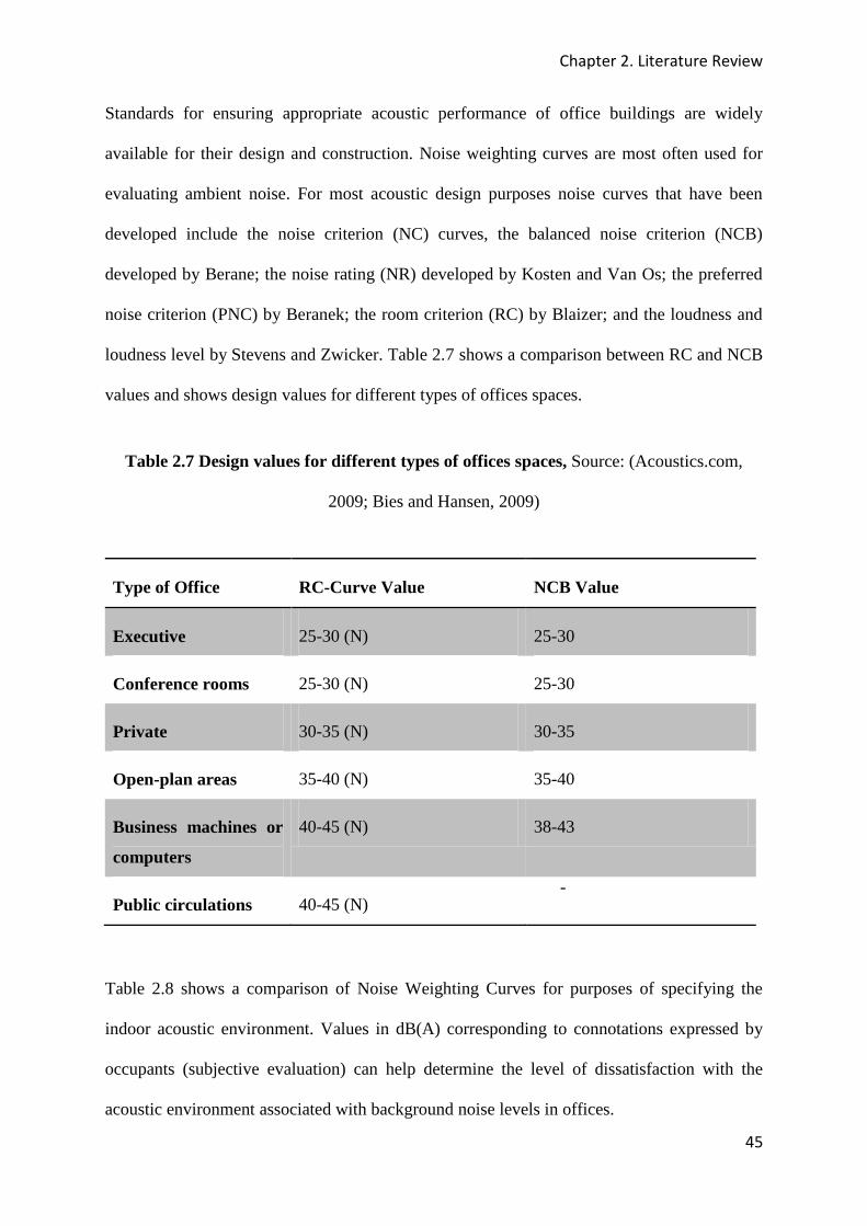
Chapter 2. Literature Review
45
Standards for ensuring appropriate acoustic performance of office buildings are widely
available for their design and construction. Noise weighting curves are most often used for
evaluating ambient noise. For most acoustic design purposes noise curves that have been
developed include the noise criterion (NC) curves, the balanced noise criterion (NCB)
developed by Berane; the noise rating (NR) developed by Kosten and Van Os; the preferred
noise criterion (PNC) by Beranek; the room criterion (RC) by Blaizer; and the loudness and
loudness level by Stevens and Zwicker. Table 2.7 shows a comparison between RC and NCB
values and shows design values for different types of offices spaces.
Table 2.7 Design values for different types of offices spaces, Source: (Acoustics.com,
2009; Bies and Hansen, 2009)
Type of Office RC-Curve Value NCB Value
Executive 25-30 (N) 25-30
Conference rooms 25-30 (N) 25-30
Private 30-35 (N) 30-35
Open-plan areas 35-40 (N) 35-40
Business machines or
computers
40-45 (N) 38-43
Public circulations 40-45 (N) -
Table 2.8 shows a comparison of Noise Weighting Curves for purposes of specifying the
indoor acoustic environment. Values in dB(A) corresponding to connotations expressed by
occupants (subjective evaluation) can help determine the level of dissatisfaction with the
acoustic environment associated with background noise levels in offices.
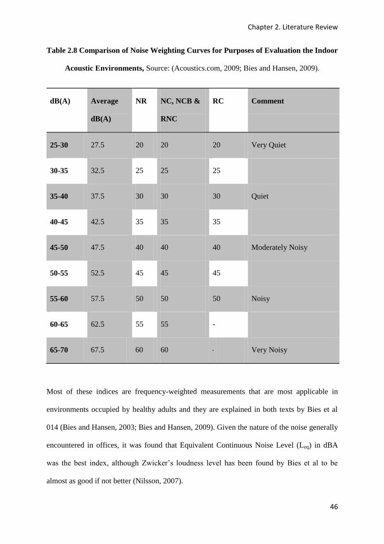
Chapter 2. Literature Review
46
Table 2.8 Comparison of Noise Weighting Curves for Purposes of Evaluation the Indoor
Acoustic Environments, Source: (Acoustics.com, 2009; Bies and Hansen, 2009).
dB(A) Average
dB(A)
NR NC, NCB &
RNC
RC Comment
25-30 27.5 20 20 20 Very Quiet
30-35 32.5 25 25 25
35-40 37.5 30 30 30 Quiet
40-45 42.5 35 35 35
45-50 47.5 40 40 40 Moderately Noisy
50-55 52.5 45 45 45
55-60 57.5 50 50 50 Noisy
60-65 62.5 55 55 -
65-70 67.5 60 60 - Very Noisy
Most of these indices are frequency-weighted measurements that are most applicable in
environments occupied by healthy adults and they are explained in both texts by Bies et al
014 (Bies and Hansen, 2003; Bies and Hansen, 2009). Given the nature of the noise generally
encountered in offices, it was found that Equivalent Continuous Noise Level (Leq) in dBA
was the best index, although Zwicker’s loudness level has been found by Bies et al to be
almost as good if not better (Nilsson, 2007).
Chapter 2. Literature Review
47
2.6 LIGHTING (VISUAL) COMFORT
2.6.1 Overview of Lighting in Office Buildings
Light is defined as the electromagnetic radiation that stimulates our visual response and
therefore helps us determine our perception of the indoor environment (Zelinsky, 2011).
Illuminance is defined in the CIBSE handbook as the ratio of the light flux (lumen) to the
illuminated surface area (m2) and is quoted in lumens per meter or lux (CIBSE, 1994). The
human visual system is part of the central nervous system (CNS) that processes surrounding
information by capturing and processing visible light (Ganong, 2003, CIBSE, 2006). The
system responds physiologically to the luminance distribution in the field of view and this
helps occupants perceive the lighting environment. More information of visual perception can
be found in literature (Malik, 2004; Ganong, 2003; Zelinsky, 2011).
Lighting quality has been defined by Chung and Burnett (2000) as “a term used to describe
all of the factors in a lighting installation that affect human comfort, health and well being”.
In order to provide a comfortable lighting environment factors such as illuminance,
illumination uniformity, luminance distribution, colour characteristics (rendering and
appearance), day lighting factors, room surface reflectance, glare and flicker rates need to be
in the right balance. Recommended values for these parameters are shown in tables later in
this chapter. Lighting installations need to be assessed for their ability to provide comfortable
indoor environments in office buildings and lighting indices are required for that purpose. A
strong link between lighting quality and work performance is also highlighted in most recent
studies (Chung and Burnett, 2000; Ratcliffe and Day, 2003).

Chapter 2. Literature Review
48
Although there is undisputed evidence of this correlation very little is known about the causal
relationships between lighting and occupant comfort, performance, or health and well being.
For example a window location is reported by Hartkopf as one of the main influences on an
occupant’s degree of satisfaction with the indoor environment with incidences of health
complaints reduced by 20-25% (Hartkopf, 2003).
There is currently very limited literature available on the development of lighting indices for
office buildings and most office lighting designs rely on lighting guides (e.g. CIBSE, 1994,
CIBSE, 2006; ASHRAE, 1999; Howley, 1999) and standards e.g. (EN12464, 2002; EN
15251, 2006). Quoting from Chung and Burnet “any general agreement on how the lighting
quality should be defined does not exist” therefore horizontal illumination of surfaces has
acted as an acceptable guide for offices and this relates to the amount of light falling on a
working plane (Chung and Burnett, 2000). Although the quantity of light falling on the
working plane (illumination) is generally accepted as an indicator of lighting quality, it only
forms a part of many contributing factors to lighting quality.
Saunders carried out studies on the effects of the level of task illuminance on quality of
lighting perceived by occupants and found a positive correlation between the two (Saunders,
1969). This relationship has stood the test of time and has been presented in many lighting
handbooks including the CIBSE code for interior lighting (CIBSE, 1994). Several other
studies have used illuminance as an indicator of lighting, for example, Linhart (2011)
performed experiments to determine the effect of energy efficient lighting on the visual
performance of 20 individuals carrying out computer tasks during an evening and used
illuminance levels as a measure of the amount of lighting received on working planes. That
study showed that relationships between illuminance and occupant acceptance of the lighting
environment exist.

Chapter 2. Literature Review
49
Some studies have used illuminance and glare to compare the visual performance of office
buildings and one such study was carried out to evaluate visual comfort in highly luminous
offices environments receiving high solar radiations (Ochoa and Capeluto, 2006). A study by
Yun et al on occupants of open plan offices revealed that there were close relationships
between prevailing illuminance levels on the work plane and luminous comfort (Yun et al,
2010). Perhaps the most ideal approach is to develop a single index that takes into account
various aspects of lighting such as illumination uniformity, luminance, distribution, colour
characteristics, room surface reflectance, glare and flicker rates. The closest to such an index
is the Comfort, Satisfaction and Performance (CSP) index developed by Bean and Bell
(1992).
The CSP index was developed as the attempt to find an index or indicator of lighting quality
intensified in the 1990s. The model assumes that there is an interaction between the three
elements of visual quality and these are comfort (C*), satisfaction (S*), and performance
(P*). According to Bean and Bell the comfort (C*) element is related to the glare index and is
given a maximum value of 10 when the glare index is less or equal to 14. The satisfaction
(S*) element is derived from the multiplication of the ratio of cylindrical illumination to
horizontal illumination by a factor of 15. S is equal to 10 when this ratio is greater or equal to
2/3. The performance (P*) element is a complex derivative of the horizontal illumination, the
ratio of cylindrical to horizontal illumination, the uniformity and colour rendering index.
Each of the elements if given a value between 0 and 10, then the CSP index has values
between 0 and 100 (Bean and Bell, 1992). The CSP index is given as:
ぬ 抜 系茅鯨茅鶏茅岫系茅 髪 鯨茅 髪 鶏茅岻 に┻な
Chapter 2. Literature Review
50
A different calculation criterion is used for offices with video display units (VDU) and this
method is explained by Bean and Bell (1992), and in Chung and Burnett (2000).
Chung (2000) also found a poor correlation between subjective assessment of the lighting
environment and the CSP index among occupants of a retrofit building in Hong Kong. The
reason for the poor performance of the index is that it is based on measurable photometric
data and hence it does not take into account most human behavioural factors. This method
therefore cannot be accepted solely as an indicator of lighting quality hence it needs to be
complemented by subjective assessment.
2.7 CURRENT STANDARDS IN OPERATION OF OFFICES
2.7.1 Recommended Criteria for the Thermal Operation of Mechanically Ventilated
Buildings
The EN ISO 7730 (2005) standard proposes that criteria for the design of thermal
environment shall be based on thermal comfort indices, i.e. the PMV-PPD (Predicted Mean
Vote - Predicted Percentage of Dissatisfied), with assumed typical activity levels and clothing
values for winter and summer. Using a reasonably assumed combination of activity and
clothing levels, an assumed relative humidity (approximately 50%) at low air velocities, it is
possible to establish a corresponding range of operative temperatures and therefore express
comfort categories as a temperature range. Operative temperatures have a significant impact
on the amount of energy used in the office therefore mechanically ventilated offices have
been classified into categories based on summer and winter design operative temperatures as
shown in Table 2.10. Recommended comfort categories based on PPD are illustrated in Table
2.9. The importance of relative humidity, air speed and air conditioning on improving thermal
comfort in mechanically ventilated buildings is discussed in the next sections.
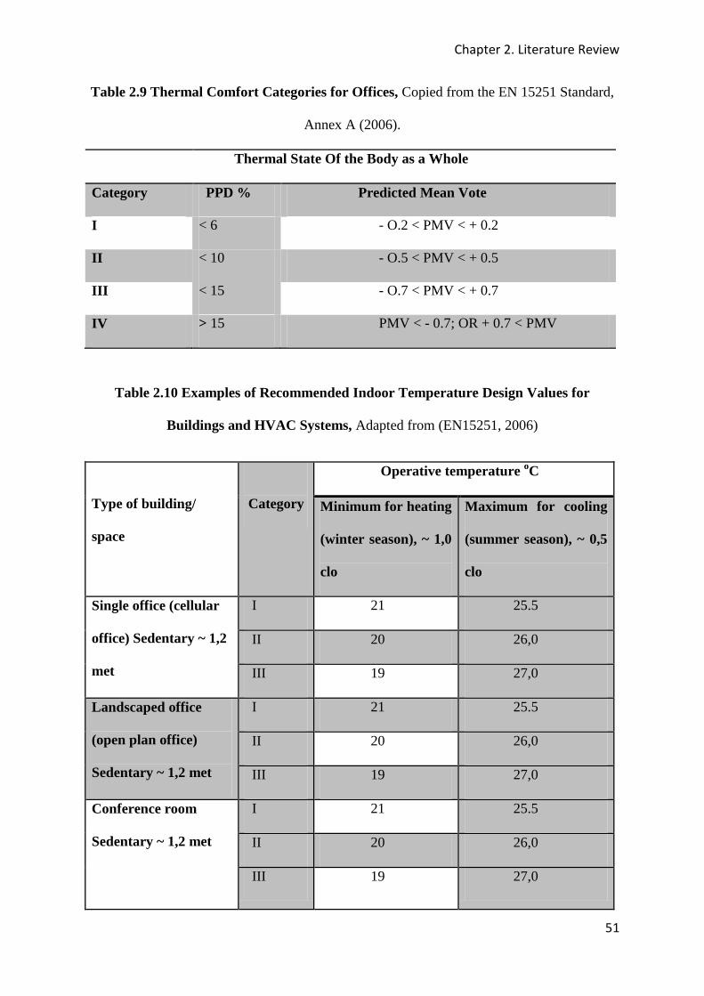
Chapter 2. Literature Review
51
Table 2.9 Thermal Comfort Categories for Offices, Copied from the EN 15251 Standard,
Annex A (2006).
Thermal State Of the Body as a Whole
Category PPD % Predicted Mean Vote
I < 6 - O.2 < PMV < + 0.2
II < 10 - O.5 < PMV < + 0.5
III < 15 - O.7 < PMV < + 0.7
IV > 15 PMV < - 0.7; OR + 0.7 < PMV
Table 2.10 Examples of Recommended Indoor Temperature Design Values for
Buildings and HVAC Systems, Adapted from (EN15251, 2006)
Type of building/
space
Category
Operative temperature oC
Minimum for heating
(winter season), ~ 1,0
clo
Maximum for cooling
(summer season), ~ 0,5
clo
Single office (cellular
office) Sedentary ~ 1,2
met
I 21 25.5
II 20 26,0
III 19 27,0
Landscaped office
(open plan office)
Sedentary ~ 1,2 met
I 21 25.5
II 20 26,0
III 19 27,0
Conference room
Sedentary ~ 1,2 met
I 21 25.5
II 20 26,0
III 19 27,0
Chapter 2. Literature Review
52
Mean Radiant Temperature (MRT)
Mean radiant temperature represents the radiant energy exchange between the human
occupant and the surfaces around and it is defined in Fanger’s textbook on thermal comfort
(Fanger, 1973) as “the uniform temperature of the surface of an imaginary enclosure where
the radiant exchange of heat between this enclosure and a man would be equal to the radiant
exchanges in the actual environment”. Occupant thermal comfort depends significantly on the
balance of radiation exchange between them and the surrounding surfaces.
When all surfaces in a room are at the same temperature, mean radiant temperature remains
uniform throughout the room. However, in some cases surface temperature may vary from
one surface to another, resulting in variation in operative temperature (resultant temperature)
(CIBSE, 1986). Mean radiant temperature may be higher or lower than the air temperature in
a room although in most cases the two are regarded as the same for thermal comfort
calculation purposes. It is measured using a Globe thermometer which consists of a thin-
walled copper sphere painted black and containing a thermometer with its bulb at the centre
of the sphere. The thermometer is suspended in the room and allowed to reach thermal
equilibrium with its surroundings (about 20 minute’s time). The equilibrium temperature
depends on both convection and radiation transfer between the sphere and the surrounding
surfaces.

Chapter 2. Literature Review
53
Air Velocity
Moving air has a cooling effect on the human skin therefore increased air velocity can be
used to compensate for increased temperatures inside buildings under summer conditions
(operative temperatures > 25°C). Fans have been used for many years as a quick solution to
local thermal discomfort in naturally ventilated buildings and to provide personalized thermal
comfort in mechanically ventilated buildings equipped with Personalized Ventilation Systems
(PVS). However higher air velocities are known to cause draughts and feelings of local
discomfort in offices and other buildings therefore control of air speed is important. The
effects of air velocities on thermal comfort (above and below set temperatures) will be
discussed further in Chapter 6, Section 6.1.1.
The upper limits of neutral temperatures in naturally ventilated office (Figure 2.8) can be
increased by a few degrees in correlation with increased fan speeds. Figure 2.4 shows the air
velocity (Va) required to offset increased temperature (CIBSE, 1986; EN15251, 2006;
ASHRAE, 1984). The curves are plots of differences between tmrt and ta while the x-axis
represents the temperature rise (∆t) above a set point of 26°C (This should depend on the
climate of the area).
For occupants performing light primarily sedentary activity temperature rise (∆t) must be
below 3°C and air velocity below 0.82 m/s as bound by the blue lines and the axes. Beyond
the lines the model cannot guarantee reliable estimations. Figure 2.8 also shows that the
larger the tmrt (or the smaller the ta), the lower the air velocities required to offset temperature
changes (Parsons, 2008).
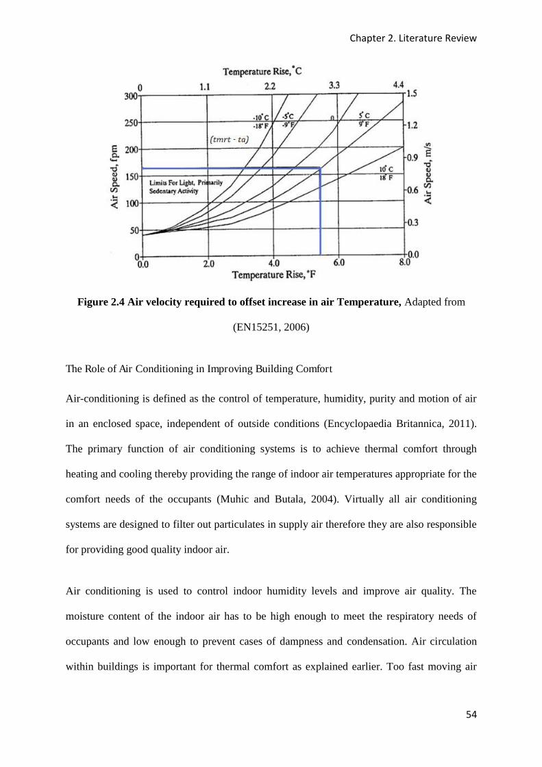
Chapter 2. Literature Review
54
Figure 2.4 Air velocity required to offset increase in air Temperature, Adapted from
(EN15251, 2006)
The Role of Air Conditioning in Improving Building Comfort
Air-conditioning is defined as the control of temperature, humidity, purity and motion of air
in an enclosed space, independent of outside conditions (Encyclopaedia Britannica, 2011).
The primary function of air conditioning systems is to achieve thermal comfort through
heating and cooling thereby providing the range of indoor air temperatures appropriate for the
comfort needs of the occupants (Muhic and Butala, 2004). Virtually all air conditioning
systems are designed to filter out particulates in supply air therefore they are also responsible
for providing good quality indoor air.
Air conditioning is used to control indoor humidity levels and improve air quality. The
moisture content of the indoor air has to be high enough to meet the respiratory needs of
occupants and low enough to prevent cases of dampness and condensation. Air circulation
within buildings is important for thermal comfort as explained earlier. Too fast moving air
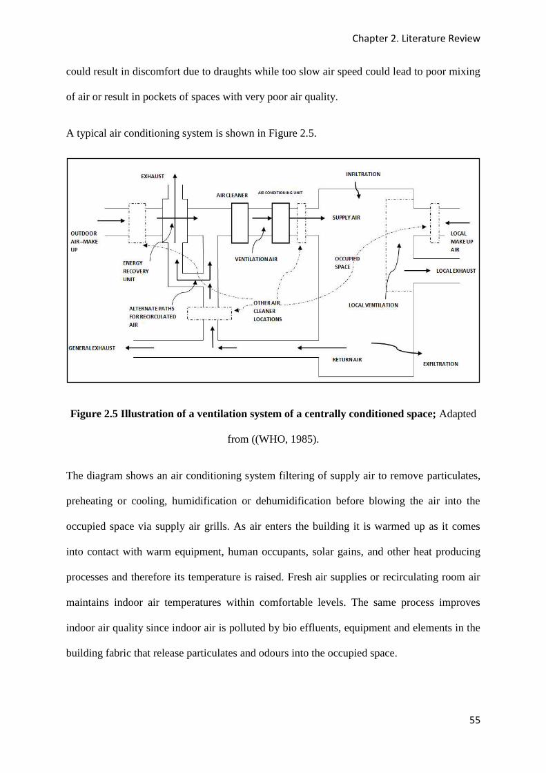
Chapter 2. Literature Review
55
could result in discomfort due to draughts while too slow air speed could lead to poor mixing
of air or result in pockets of spaces with very poor air quality.
A typical air conditioning system is shown in Figure 2.5.
Figure 2.5 Illustration of a ventilation system of a centrally conditioned space; Adapted
from ((WHO, 1985).
The diagram shows an air conditioning system filtering of supply air to remove particulates,
preheating or cooling, humidification or dehumidification before blowing the air into the
occupied space via supply air grills. As air enters the building it is warmed up as it comes
into contact with warm equipment, human occupants, solar gains, and other heat producing
processes and therefore its temperature is raised. Fresh air supplies or recirculating room air
maintains indoor air temperatures within comfortable levels. The same process improves
indoor air quality since indoor air is polluted by bio effluents, equipment and elements in the
building fabric that release particulates and odours into the occupied space.
Chapter 2. Literature Review
56
Air conditioning systems can be categorised into three main types namely:
i) Local Comfort Cooling systems;
ii) Centralised Air systems; and
iii) Partially Centralised Air/Water systems.
Typical systems can be found in the HEVACOMP knowledge base (Bentley, 2010) and other
texts.
Humidification and Dehumidification of Indoor Air
The relative humidity of air needs to be controlled to ensure thermal comfort for occupants.
Although relative humidity has a relatively small effect on thermal sensation or perceived air
quality long term high humidity could result in microbial growth and poor IAQ. Low
humidity is associated with drying of the skin, eyes and airways. Research shows that human
occupants are likely to accept a higher temperature at a lower humidity than the same
temperature at a higher humidity (Fiala, 2008; Fanger, 1973; Toftum and King, 2002). A
criterion for humidification or dehumidification depends on thermal comfort and air quality
requirements of the building. The design of humidification and dehumidification equipment
has a bearing on the energy performance of a building.
Dehumidification of indoor air is achieved via two processes; (1) cooling air temperature
below dew point in order to dump moisture and (2) chemical adsorption. Cooling air below
dew point is an energy intensive process that involves passing air over a cold coil in the air
handling unit. This causes some of the air to condense and the amount of moisture removed
depends on the temperature of the coil and the air flow rates across the coil. Air then needs to

Chapter 2. Literature Review
57
be reheated to bring it back to the required comfort temperature (ASHRAE, 1984, 1985).
Using an evaporator and condenser coil saves energy since only compressor power is needed
for both cooling and heating in the dehumidification cycle.
A typical dehumidification air conditioning cycle is shown in Figure 2.6 below.
Figure 2.6 An illustration of a dehumidification system that involves cooling air below
dew point, Adapted from (ASHRAE, 1985)
Chemical sorption involves the use of desiccants to remove water vapour from air. Most
desiccant systems are based on a slow rotating desiccant rotor, which is a solid wheel (Figure
2.7) that is packed with solid desiccant materials. Air is forced through the dehumidification
section of the wheel where moisture is absorbed and the desiccant becomes saturated. The
desiccant wheel goes through a regeneration process where heated air is forced through it to
remove moisture. This method is less energy intensive compared to the dew point approach.
A typical desiccant wheel is shown in Figure 2.7.
Evaporator Coil Condenser Coil Duct
Warm Humid
Air Cold Dry Air Warm Dry Air
Condensate
Drain
Compressor Expansion Valve

Chapter 2. Literature Review
58
Figure 2.7 Desiccant based dehumidification system, Adapted from: (Fang et al, 2005)
Design values for humidity levels required for most buildings including offices are shown in
Table 2.11. Different design limits are required for special environments such as process
areas, museums and churches where humidity plays an important role in the preservation of
equipment and materials.
Table 2.11 Example of Recommended Design Criteria for the Relative Humidity in
Occupied Spaces Where Humidification or Dehumidification Systems are Installed
Source: (EN15251, 2006)
Type of
building/space Category Design RH for
dehumidification, %
Design RH for
humidification, %
Spaces where
humidity criteria are
set by human
occupancy.
I 50 30
II 60 25
III 70 20
IV >70 <20
Reactivation Air
Dry Air
Wet Air
Process Air

Chapter 2. Literature Review
59
2.7.2 Criteria for the thermal operation of naturally ventilated buildings – Adaptive
Comfort
A different indoor environment criterion exists for offices without mechanical ventilation i.e.
naturally ventilated offices because occupants tend to adapt to the indoor environment based
on outdoor conditions. Figure 2.8 is an example of recommended design indoor operative
temperatures and categories for naturally ventilated offices in the UK (Auliciems, 1981). The
operative temperatures (room temperatures) presented in the graph below are valid for offices
and other buildings of similar type where occupants carry out mainly sedentary activities,
have easy access to operable windows and they may freely adapt their clothing or any other
aspects that may improve their comfort depending on the indoor and/or outdoor thermal
conditions (Humphreys, 1994). This method is therefore strictly used in naturally ventilated
spaces where no mechanical heating or cooling exists otherwise the methodology does not
apply during periods when the heating or cooling systems are operational.
Figure 2.8 Recommended design indoor operative temperatures for naturally ventilated
offices in the UK using the Auliciems Model, Copied from deDear and Brager (2001).
Chapter 2. Literature Review
60
In most naturally ventilated spaces people often tolerate their indoor environment, for
example, higher operative temperatures can be acceptable in warmer climates than in colder
ones hence higher PMV values than expected are usually observed. However studies by
Fanger (1986) made a distinction between adaptation and tolerance. He suggested that people
cannot adapt to preferring warmer or colder temperatures, but they may tolerate the situation
better than others from a different climate.
The quality of the thermal environment in naturally ventilated buildings also depends on
outdoor thermal conditions. The building envelope provides an interface between the two and
the choice of building materials and building orientation has a remarked effect on what is
perceived inside the building. Clothing levels in different parts of the world tend to suggest a
response to outdoor thermal conditions as people in warm or cold climates tend to tolerate
uncomfortably high or low temperatures by maintaining relatively higher levels of
performance at under those conditions.
2.7.3 IAQ and Ventilation Standards
Air is supplied to office buildings through passive and active ventilation systems. Passive
systems supply air into the building through thermal stack effects or take advantage of wind
power which pushes air into the building via windows or air vents. Mechanical ventilation
systems are active ventilation systems which are mainly powered by grid electricity and they
include mixing, displacement and personalised ventilation systems (PVS). The systems are
responsible for maintaining the required IAQ standards in offices and fresh air needs
throughout the occupancy periods if good air quality standards are to be achieved.

Chapter 2. Literature Review
61
In some cases air supply into the building may even start before occupancy begins in order to
avoid that “warm up” period that may be responsible for many building related illnesses. At
present there are no universally accepted standards for IAQ in the UK hence different
categories of Indoor Air Quality in buildings have been created based on the amount of
ventilation air supplied, concentrations of CO2 above outdoor and pollution levels in decipol,
as presented in Tables 2.12, 2.13 and 2.14 respectively. It is also generally accepted in most
ventilated areas that ventilation rates for comfort will cover ventilation rates for health.
Table 2.12 Air Quality Categories Based on Amount of Ventilation Air Supplied to the
Building, Source: (Commission for European Communities, 1991)
Category Expected Percentage Dissatisfied Airflow per person (l/s/person)
I 15 10
II 20 7
III 30 4
IV >30 <4
Design ventilation rates can be calculated by adding ventilation rates required for removal of
bio effluents and ventilation rates required for removal of pollution due to the building’s
fabric and its systems. In some cases ventilation rates per square metre floor area can be used
instead and the recommended values can be found in Annex B of the EN15251 standard.
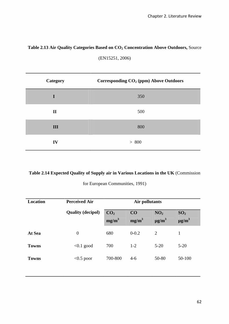
Chapter 2. Literature Review
62
Table 2.13 Air Quality Categories Based on CO2 Concentration Above Outdoors, Source
(EN15251, 2006)
Category Corresponding CO2 (ppm) Above Outdoors
I 350
II 500
III 800
IV > 800
Table 2.14 Expected Quality of Supply air in Various Locations in the UK (Commission
for European Communities, 1991)
Location Perceived Air
Quality (decipol)
Air pollutants
CO2
mg/m3
CO
mg/m3
NO2
µg/m3
SO2
µg/m3
At Sea
Towns
Towns
0
<0.1 good
<0.5 poor
680
700
700-800
0-0.2
1-2
4-6
2
5-20
50-80
1
5-20
50-100
Chapter 2. Literature Review
63
Annex C of the EN 15251 standard provide guidelines on how to define low and very low
polluting buildings. The standard states that safe and low polluting building materials must
fulfil the following requirements:
The emission of total volatile organic compounds (TVOC) is below 0.2 mg/m²h;
The emission of formaldehyde is below 0.05 mg/m²h;
The emission of ammonia is below 0.03 mg/m²h;
The emission of carcinogenic compounds (IARC) is below 0.005 mg/m²h; and
The material is not odorous (dissatisfaction with the odour is below 15 %).
More information on indoor air quality standards and exposure limits to indoor pollutants can
be found in the WHO - Environmental Health Criteria (EHC) documents (WHO, 1994).
2.7.4 Criteria for Acoustic Operation of Office Buildings
An important aspect of acoustic comfort is to establish criteria for the indoor environment.
Thus where total elimination of noise in offices is impractical, appropriate guidelines must be
set to determine how much noise is acceptable. Also it is important to determine how noise
levels impact on the performance of office occupants, and how noise reduction strategies
impact on the energy bill. Table 2.15 gives some examples of ranges of acceptable A-
weighted indoor sound levels in office buildings. A full list of maximum acceptance A-
weighted sound pressure levels for various buildings can be found on the Australian and New
Zealand standards, AS2107 (Australian Standard, 1987, Australian & New Zealand Standard,
2000).
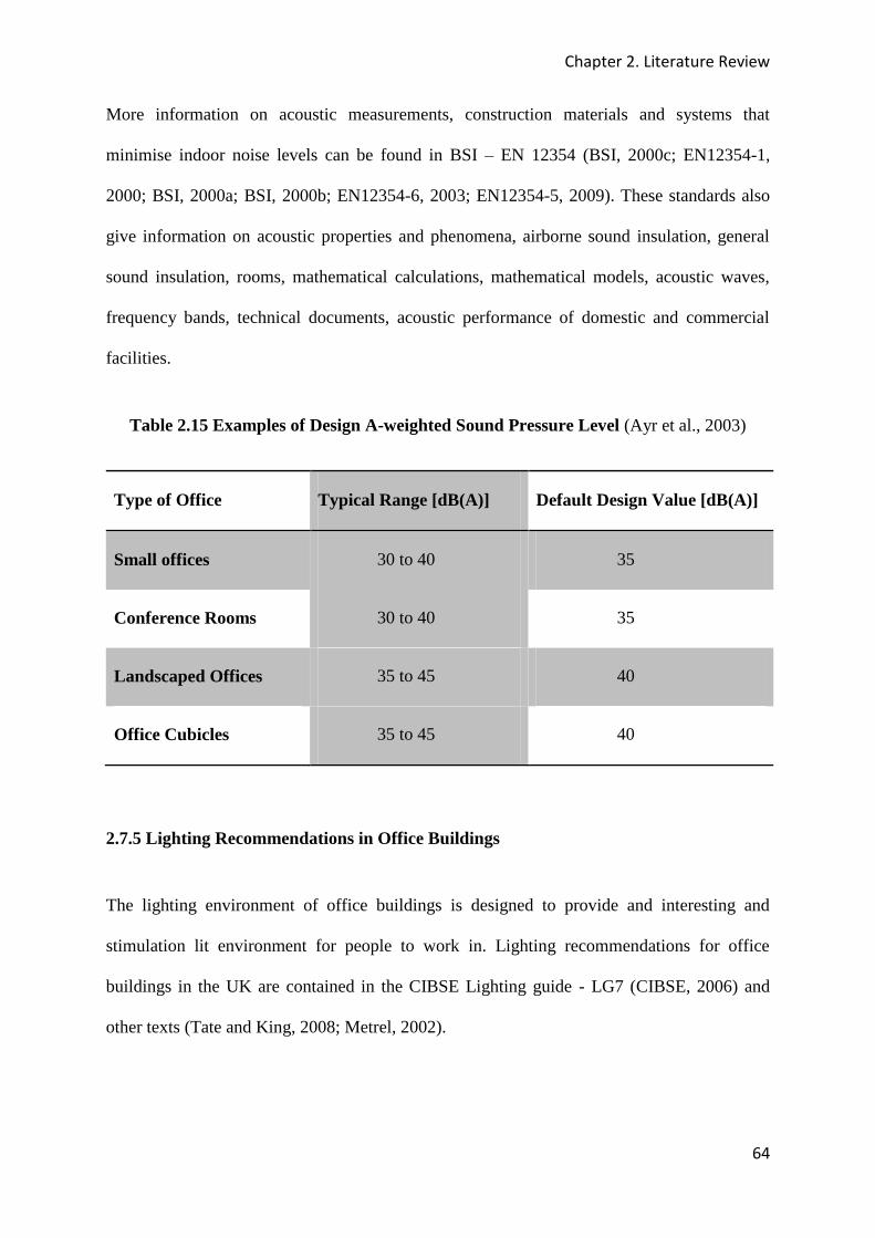
Chapter 2. Literature Review
64
More information on acoustic measurements, construction materials and systems that
minimise indoor noise levels can be found in BSI – EN 12354 (BSI, 2000c; EN12354-1,
2000; BSI, 2000a; BSI, 2000b; EN12354-6, 2003; EN12354-5, 2009). These standards also
give information on acoustic properties and phenomena, airborne sound insulation, general
sound insulation, rooms, mathematical calculations, mathematical models, acoustic waves,
frequency bands, technical documents, acoustic performance of domestic and commercial
facilities.
Table 2.15 Examples of Design A-weighted Sound Pressure Level (Ayr et al., 2003)
Type of Office Typical Range [dB(A)] Default Design Value [dB(A)]
Small offices 30 to 40 35
Conference Rooms 30 to 40 35
Landscaped Offices 35 to 45 40
Office Cubicles 35 to 45 40
2.7.5 Lighting Recommendations in Office Buildings
The lighting environment of office buildings is designed to provide and interesting and
stimulation lit environment for people to work in. Lighting recommendations for office
buildings in the UK are contained in the CIBSE Lighting guide - LG7 (CIBSE, 2006) and
other texts (Tate and King, 2008; Metrel, 2002).

Chapter 2. Literature Review
65
Lighting design in offices is based on the following aspects:
Illuminance (lux on a working plane);
Discomfort Glare (including UGR);
Colour qualities of light (including Ra); and
Directionality of lighting.
Generally office lighting is concerned with the provision of uniform lighting across each task
area. Task areas consist of relatively small areas around the workstations where visual tasks
are carried out. The immediate surrounding area is the area surrounding the task area within
the visual field and this is usually a band of about 0.5 metres wide around the task area. The
task area and the surrounding area are shown in Figure 2.9. Generally surrounding areas have
illuminance distributions (gi) of 半 0.5 and the task areas have gi ≥ 0.7.
Figure 2.9 Task area & immediate surrounding area, Copied from (EN12464-1, 2002)

Chapter 2. Literature Review
66
The selection of the type of lighting suitable for an office space depends on the physical
constraints of the space, the intended decor, the capital investment intended, energy
implications, and maintenance costs. The procedure for selection of luminaries is explained in
the Lighting Guide 7, 2005 and will not be discussed here. Some recommended illuminance
values for offices are shown in Table 2.16 while typical outdoor illuminance levels are shown
in Table 2.17.
Table 2.16 Recommended Design Indoor Lighting for Offices and Other Buildings in
the UK, Source: (EN15251, 2006)
Type of Office Maintained Illuminance,
at working areas, lux
UGR Ra Height of Working
plane (m)
Single/cellular 500 19 80 0.8
Open Plan 500 19 80 0.8
Conference rooms 500 19 80 0.8
Circulation areas/stairs 150 25 40 0.1
Corridors 100 28 40 0.1
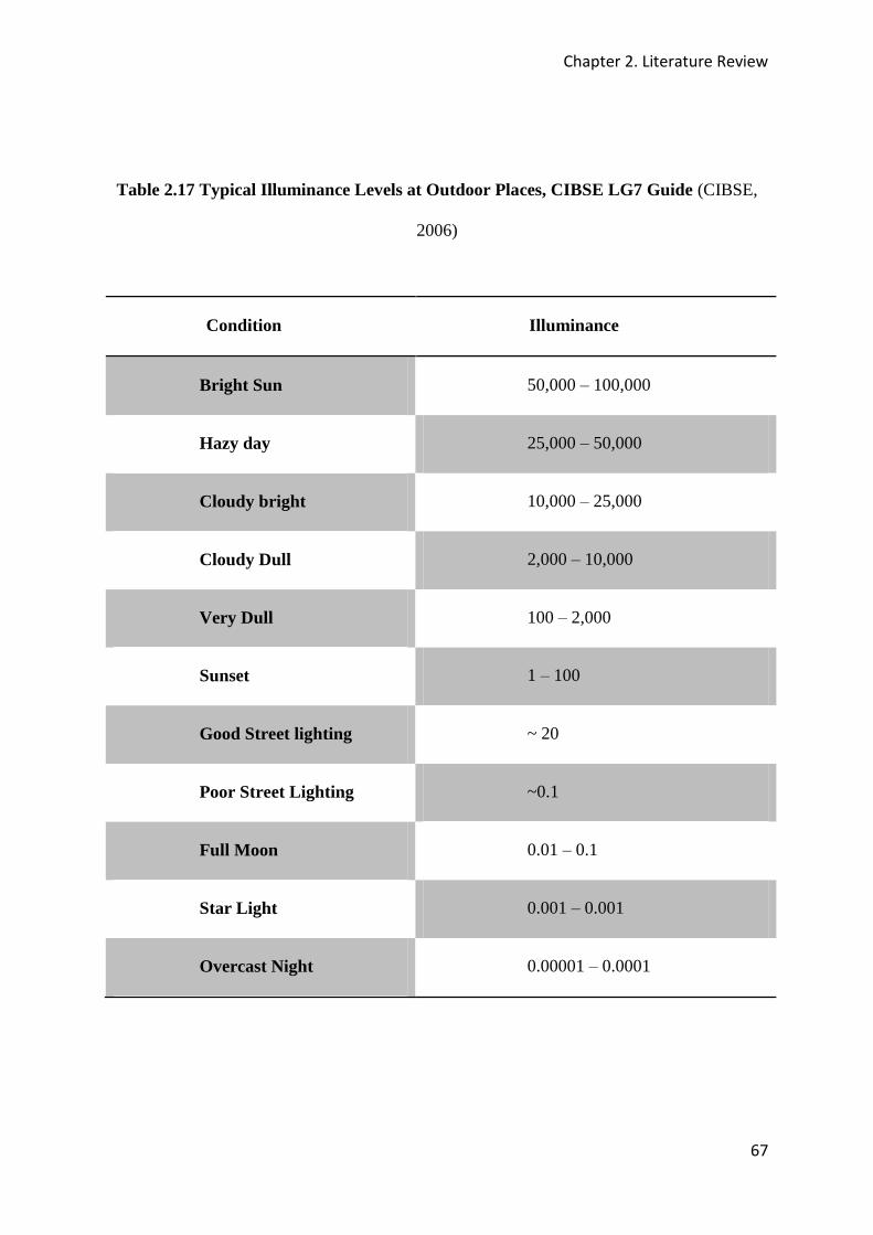
Chapter 2. Literature Review
67
Table 2.17 Typical Illuminance Levels at Outdoor Places, CIBSE LG7 Guide (CIBSE,
2006)
Condition Illuminance
Bright Sun 50,000 – 100,000
Hazy day 25,000 – 50,000
Cloudy bright 10,000 – 25,000
Cloudy Dull 2,000 – 10,000
Very Dull 100 – 2,000
Sunset 1 – 100
Good Street lighting ~ 20
Poor Street Lighting ~0.1
Full Moon 0.01 – 0.1
Star Light 0.001 – 0.001
Overcast Night 0.00001 – 0.0001
Chapter 2. Literature Review
68
The design of day lighting for offices is critical since it is a universal worker requirement as
explained earlier. UK Regulation 8(2) of the Workplace Regulations states that “the lighting
in every workspace shall, as far as reasonably practicable, be by natural light” (Energy
Information & Administration, 2006). In order to maximise the amount of natural light
received by occupants, reduce glare and save energy good lighting designs are required. One
of the simplest methods of achieving satisfactory luminance range is to avoid users looking
directly out onto potentially bright patches of sky or having windows behind them reflecting
on their screens. This includes making sure that the display screens are placed perpendicular
to the plane of the windows so that the user’s viewing axis runs parallel to the windows
(CIBSE, 2006). A recommended minimum daylight factor of 2% gives an illuminance level
of 1000 lux for much of the working year but is difficult to achieve the same for areas over
6m from the window (Chung and Burnett, 2000).
Daylight levels near to the windows can be more than ten times higher than elsewhere in the
office and this may have a profound effect on the body’s biological clock, leading to what is
commonly referred to as the Seasonal Affective Disorder (SAD). In many cases however, if
not correctly checked, the amount of day lighting could have a negative impact on the
occupants visual comfort, contribute to heat gains leading to thermal discomfort and windows
with outside views could lead to invasion of privacy (Bean and Bell, 1992). Efficient use of
day lighting could contribute significantly to reducing energy consumption in offices.
2.8 CONCLUSIONS
Office buildings are one of the main contributors of carbon emissions in the UK. In order to
tackle the effects of climate change it is essential that the energy consumption of offices is
reduced to a sustainable level. Reducing carbon emissions means operating buildings within
sustainable comfort levels. However the quest to reduce carbon emissions in office buildings
Chapter 2. Literature Review
69
should not sacrifice the comfort of those who work within those buildings. In order to help
building designers, owners and users use offices more efficiently there is need to develop
tools to help them assess the impact of their indoor environment standards on the
environment.
This can be done by developing energy and IEQ assessment methodologies that could be
compared easily. IEQ assessment methodologies rely on the ability to develop indices that
accurately evaluate thermal comfort, IAQ, acoustics and lighting comfort. Although thermal
comfort and IAQ indices are well developed lighting and acoustic comfort indices still
require extensive research. The next chapters (Chapter 3, 4 and 5) attempt to develop a
methodology for assessment of IEQ in offices based what has already been discussed in this
chapter and case studies.

Chapter 3. The IEQ Assessment Model
70
3. The IEQ Assessment Model
3.1 ITRODUCTION
This Chapter presents a methodology for the IEQAT (Indoor Environment Quality
Assessment Tool) tool for rapid assessment of IEQ in office buildings in the UK. The chapter
also explains how each of the proposed indices is developed and includes a step by step guide
on how to carry out an assessment. The tool is tested in selected case studies buildings and
the results of analysis are presented in Chapter 5. The relative weightings of each of the
contributing parameters obtained from subjective assessment will be compared to those of the
IEQAT (obtained using the AHP).
The IEQAT tool is based on the IEQ model. In the context of this thesis a single index, called
the IEQindex, is a function of four contributing environmental factors and it is explained by
means of some mathematical formula or expression. The contributing factors are sub-indices
that are associated with individual environmental aspects of the indoor environment such as
thermal comfort, IAQ, Acoustic comfort, and Lighting. The IEQindex represents perceived
IEQ; the quantity from overall perception of the quality of the indoor environment is derived
therefore it should communicate to the building designer, manager and user, the state of the
office environment relative to other similar environments in the UK. The state of the office
environment is its rating and it provides an effective framework for assessing building
performance and offers an opportunity to create high performance buildings that have less
negative impacts on occupants and the environment. The results of the tool should reflect the
advantages if any that are associated with investing in energy efficiency and therefore leave it
to the building designer, manager and user to take appropriate action where necessary.
Chapter 3. The IEQ Assessment Model
71
Three most important steps in the study include the development of the indices for assessing
each of the four proposed aspects of the indoor environment, evaluating the indices using
data obtained from case study buildings and developing a methodology to be used to derive
the relative weightings of each of the contributors.
The tool measures the following aspects (quantities) of the indoor environment:
The state of its thermal environment;
The quality of indoor air;
The quality of the acoustic environment;
The quality of the visual (lighting) environment; and
The overall (combined) state of the indoor environment.
3.2 DEVELOPMENT SOFTWARE
The tool can be developed using approved building simulation software such as MATLAB,
Simulink, Eclipse and the Visual Basic (VB) Application Programs. MATLAB is a high
level language and interactive numerical computing environment that enables one to perform
complex tasks more quickly when compared with traditional programming such as C, C++ and
FORTRAN. MATLAB allows matrix manipulations, plotting of functions and data,
implementation of algorithms, creation of user interfaces, and interfacing with programs
written in other languages, including C, C++, Java, and FORTRAN. It has been widely used
in research and industry and has been very useful in carrying out thermal comfort
assessments in office buildings (Mendes et al, 2003). Simulink, a product of MathWorks is an
additional package that can be added to MATLAB to provide a graphical multi domain
simulation capability.
Chapter 3. The IEQ Assessment Model
72
Labview is a VB language developed by National instruments. It is a smart development
environment that can be very useful for carrying out real time monitoring of the indoor
environment. It can be incorporated into the BMS and hence log in important IEQ data whilst
displaying the results in real-time. ECLIPSE is an Integrated Development Environment
(IDE) with an extensive plug in system. It can be written in many languages including Java,
C, C++ COBOL, etc and it is one of the options for the development of computer based
assessment tools. The Visual Basic (VB) program is probably the most applicable and readily
available software at the University of Nottingham. The VB program which is offered by
Microsoft Corporation is available free to student designers and developers worldwide. The
VB application is relatively easy to learn from a programmer’s point of view since most
people are familiar with interfaces associated with Microsoft and Apple applications. The
formulae used here are relatively easy to solve using basic excel and the only exception is the
thermal comfort estimation which requires a computer program.
3.3 DEVELOPING THE ASSESSMENT MODEL
The development of the IEQ assessment model begins with the identification of main
contributing factors which include thermal comfort, IAQ, acoustics and lighting. The
contributing factors constitute what is referred to as sub-indices and their development is
described in the following sections.
3.3.1 Development of Thermal Comfort sub – index (TCindex)
The thermal comfort sub index is based on Fanger’s studies in the 1970s, which constitutes
what is now known as the ISO 7730 standard (EN-ISO7730, 2005). The standard presents
methods for predicting the general thermal sensation and degree of thermal dissatisfaction
which can be expressed by a large group of people exposed to moderate thermal environments
Chapter 3. The IEQ Assessment Model
73
of mechanically ventilated and air conditioned offices. Different assessment criteria exist for
offices that are naturally ventilated and where the adaptive comfort model is used (see later
part of this section. The standard is applicable to the following situations:
Environmental conditions considered acceptable for both general and local thermal
discomfort.
Healthy men and women exposed to indoor environments where the thermal
environment plays an important part of the general comfort.
The standard does not include local discomfort factors such as draught, radiant
temperature asymmetry, vertical air temperature differences and floor or surface
temperatures. These need to be assessed separately and recommendations are
corrective measures need to be implemented to eliminate local discomfort
conditions.
ISO 7730 proposes four physical parameters that affect thermal comfort as Air temperature*,
Mean radiant temperature**, Relative Humidity*** and Air velocity; and two personal
factors as Clothing Insulation and Activity Levels. These factors have already been described
in the previous chapter (Chapter 2). Their contribution to thermal comfort is explained later in
this chapter. A flowchart for the calculation of thermal comfort is illustrated in Figure 3.1.
* Air temperature (ta) refers to the normal “room temperature” ** Mean radiant temperature (tmrt) is the uniform temperature of the surface of an imaginary enclosure where the radiant exchange of heat
between this enclosure and a man would be equal to the radiant exchanges in the actual environment (Fanger, 1973). Mean radiant temperature may be higher or lower than the air temperature in a room however in most cases it is taken as equal to air temperature (ta).
*** Relative humidity is defined as the ratio of mass of water vapour present in air at a temperature/ maximum water vapour content of that air at that temperature.

Chapter 3. The IEQ Assessment Model
74
Figure 3.1 Thermal Comfort Estimation Flowchart
Calculation of thermal comfort begins with the heat balance equation which states that in
order for the core body temperature to remain constant heat produced in the body must be
equal to heat lost from the body.
噺 惣┻ 層
Estimation of Environmental variables Estimation of Personal variables
Mean Radiant Temperature
Air Temperature
Air velocity
Relative Humidity
Clothing Insulation
Metabolic Heat Production
Predicted Mean Vote
Predicted Percentage Dissatisfied
Thermal Comfort Index
Chapter 3. The IEQ Assessment Model
75
In other words heat retention (which affects core body temperature) is 0 when metabolic heat
production is cancelled out by losses due to external work, heat loss due to conduction,
convection, radiation, evaporation and respiration as shown in equation 3.2.
警 髪 激 伐 継 伐 系 伐 迎 伐 計 伐 迎継鯨 噺 惣┻ 匝
More information on the development of the equation (s) can be found in Fanger’s textbook
on thermal comfort (Fanger, 1973). In this thesis the most relevant equation for thermal
comfort calculation is the comfort equation which is given as follows:
茎 伐 ど┻ぬな 抜 岫のば┻ね 抜 ど┻どば 抜 茎 伐 鶏銚岻 伐 ど┻ねに 抜 岫茎 伐 のぱ岻 伐 ど┻どどなば 抜 警 抜 岫のぱ┻ば 伐 鶏銚岻伐 ど┻どどなね 抜 警 抜 岫ぬね 伐 建銚岻噺 ぬ┻ひ 抜 など貸腿 抜 血頂鎮 抜 岶岫建頂鎮 髪 にばぬ岻 伐 岫建陳追痛 髪 にばぬ岻替 岼 髪 血頂鎮 抜 月頂抜 岫建頂鎮 伐 建銚岻 惣┻ 惣
Where: H = M – W and;
建潔健 噺 ぬの┻ば 伐 ど┻どにばの 抜 茎 髪 ど┻なのの荊頂鎮 抜抜 岶茎 伐 ど┻ぬな 抜 岫のば┻ね 伐 ど┻どば 抜 茎 伐 鶏銚岻 伐 ど┻ねに抜 岫茎 伐 のぱ岻 伐 ど┻どどなば 抜 警 抜 岫のぱ┻ば 伐 鶏銚岻 伐 ど┻どどなね 抜 警 抜 岫ぬね 伐 建頂鎮岻岼 惣┻ 想
And;
月頂 噺 崕に┻ぬぱ 岫建頂鎮 伐 建銚岻待┻態泰 血剣堅 に┻ぬぱ 岫建頂鎮 伐 建銚岻待┻態泰 伴 なに┻なヂ撃欠堅なに┻なヂ撃欠堅 血剣堅 に┻ぬぱ岫建頂鎮 伐 建銚岻待┻態泰 隼 なに┻な ヂ撃欠堅 惣┻ 捜 血潔健 噺 犯な┻どど 髪 ど┻に荊頂鎮 荊頂鎮 隼 ど┻の 潔健剣な┻どの 髪 ど┻な荊頂鎮 荊頂鎮 伴 ど┻の 潔健剣 惣┻ 掃
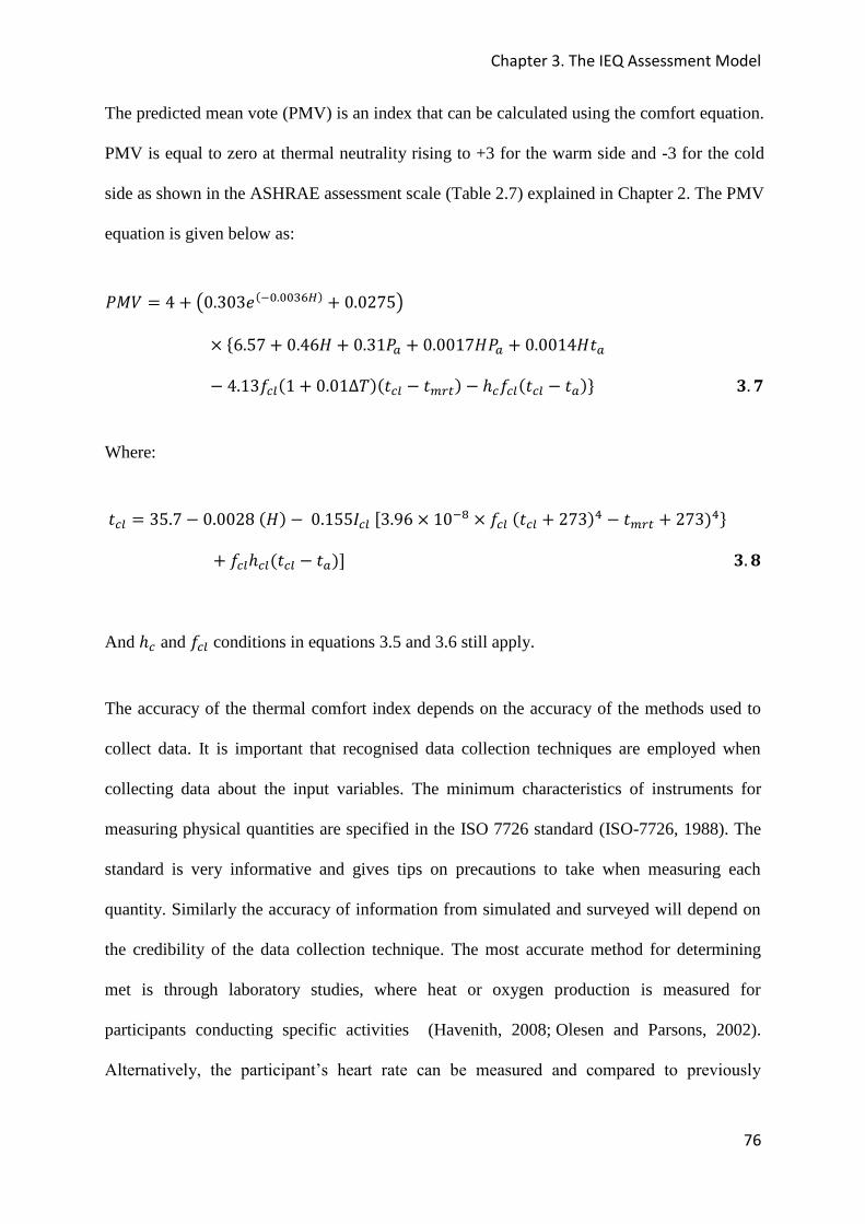
Chapter 3. The IEQ Assessment Model
76
The predicted mean vote (PMV) is an index that can be calculated using the comfort equation.
PMV is equal to zero at thermal neutrality rising to +3 for the warm side and -3 for the cold
side as shown in the ASHRAE assessment scale (Table 2.7) explained in Chapter 2. The PMV
equation is given below as:
鶏警撃 噺 ね 髪 盤ど┻ぬどぬ結岫貸待┻待待戴滞張岻 髪 ど┻どにばの匪抜 岶は┻のば 髪 ど┻ねは茎 髪 ど┻ぬな鶏銚 髪 ど┻どどなば茎鶏銚 髪 ど┻どどなね茎建銚伐 ね┻なぬ血頂鎮岫な 髪 ど┻どなッ劇岻岫建頂鎮 伐 建陳追痛岻 伐 月頂血頂鎮岫建頂鎮 伐 建銚岻岼 惣┻ 挿
Where:
建頂鎮 噺 ぬの┻ば 伐 ど┻どどにぱ 岫茎岻 伐 ど┻なのの荊頂鎮 岷ぬ┻ひは 抜 など貸腿 抜 血頂鎮 岫建頂鎮 髪 にばぬ岻替 伐 建陳追痛 髪 にばぬ岻替岼髪 血頂鎮月頂鎮岫建頂鎮 伐 建銚岻峅 惣┻ 掻
And 月頂 and 血頂鎮 conditions in equations 3.5 and 3.6 still apply.
The accuracy of the thermal comfort index depends on the accuracy of the methods used to
collect data. It is important that recognised data collection techniques are employed when
collecting data about the input variables. The minimum characteristics of instruments for
measuring physical quantities are specified in the ISO 7726 standard (ISO-7726, 1988). The
standard is very informative and gives tips on precautions to take when measuring each
quantity. Similarly the accuracy of information from simulated and surveyed will depend on
the credibility of the data collection technique. The most accurate method for determining
met is through laboratory studies, where heat or oxygen production is measured for
participants conducting specific activities (Havenith, 2008; Olesen and Parsons, 2002).
Alternatively, the participant’s heart rate can be measured and compared to previously

Chapter 3. The IEQ Assessment Model
77
developed tables of heart rate for specific activities. All of the methods mentioned above,
however, are time-consuming and invasive, and are generally not practical for use by most
thermal comfort researchers. Instead, these researchers rely on estimates based on tables of
met rates for specific activities and occupations that are developed from laboratory studies
(ASHRAE, 2005; Fanger, 1973). In most studies, an average met rate is assumed for the
group (usually 1.2 met for sedentary office work). More recent studies ask occupants to
record activities carried out in the last hour, with this information being used to develop a
more accurate average for the group, or individualised met estimates for each participant
(Cena, 1994). Methods for estimating metabolic heat production are described in the ISO
8996 standard (1989). Simpler tables comparing heat production to activity levels have been
developed and they are commonly used for the general assessment of metabolic heat
production. Table 3.1 is a summary of met values for people doing typical office tasks.
Table 3.1 Metabolic Rates for Typical Tasks (Fanger, 1973)
Activity Metabolic Rate (met)
Reclining 0.8
Seated, quietly 1.0
Sedentary activity (office, dwelling, lab, school) 1.2
Standing, relaxed 1.2
Light activity, standing (shopping, lab, light industry) 1.6
Medium activity, standing (shop assistant, domestic, etc) 2.0
High activity (heavy machine work, garage work) 3.0
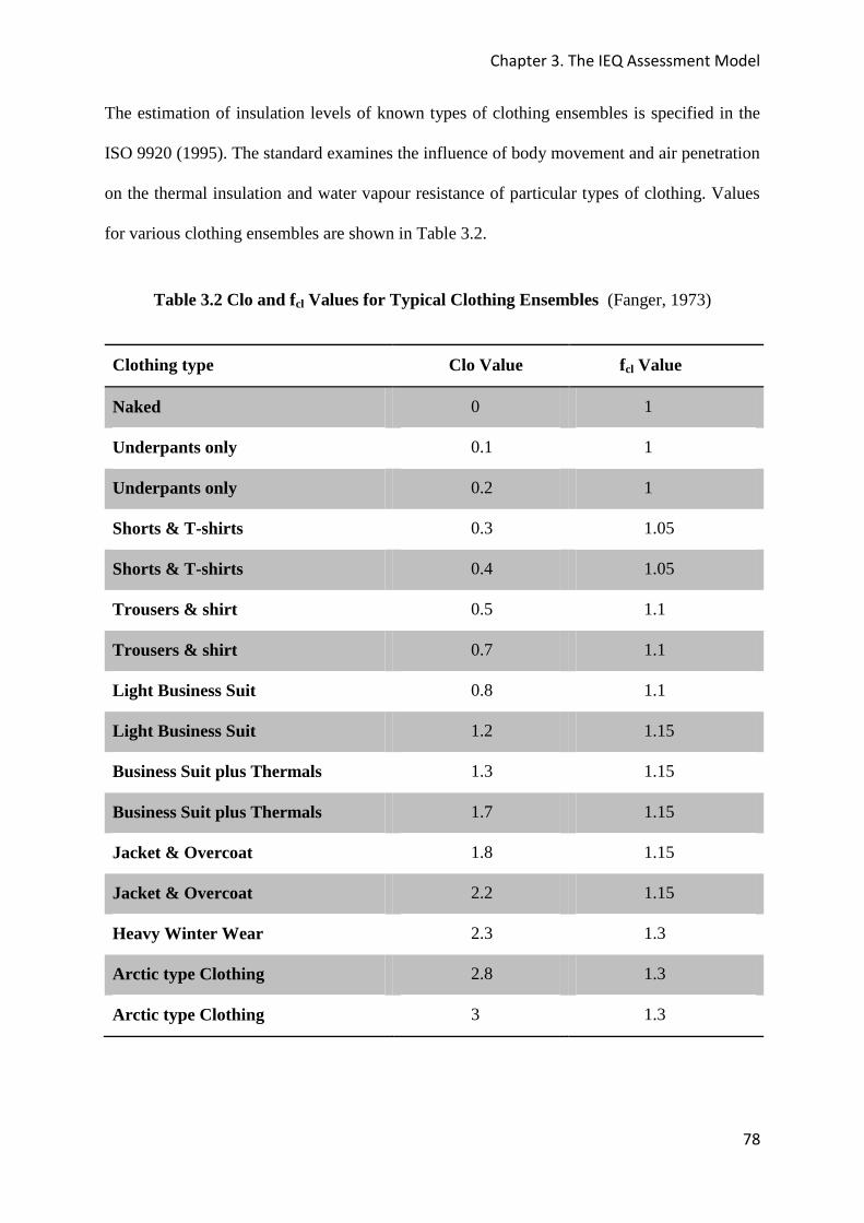
Chapter 3. The IEQ Assessment Model
78
The estimation of insulation levels of known types of clothing ensembles is specified in the
ISO 9920 (1995). The standard examines the influence of body movement and air penetration
on the thermal insulation and water vapour resistance of particular types of clothing. Values
for various clothing ensembles are shown in Table 3.2.
Table 3.2 Clo and fcl Values for Typical Clothing Ensembles (Fanger, 1973)
Clothing type Clo Value fcl Value
Naked 0 1
Underpants only 0.1 1
Underpants only 0.2 1
Shorts & T-shirts 0.3 1.05
Shorts & T-shirts 0.4 1.05
Trousers & shirt 0.5 1.1
Trousers & shirt 0.7 1.1
Light Business Suit 0.8 1.1
Light Business Suit 1.2 1.15
Business Suit plus Thermals 1.3 1.15
Business Suit plus Thermals 1.7 1.15
Jacket & Overcoat 1.8 1.15
Jacket & Overcoat 2.2 1.15
Heavy Winter Wear 2.3 1.3
Arctic type Clothing 2.8 1.3
Arctic type Clothing 3 1.3

Chapter 3. The IEQ Assessment Model
79
The PMV equation is a long and complex equation that is difficult to solve by hand and
therefore it can be better solved by using a computer program and some of the results of the
solutions have been plotted in comfort diagrams that are widely available in many texts
(Fanger, 1973). A VB code has been developed for thermal comfort calculations and it is
found in Appendix 1.
The Predicted Percentage Dissatisfied (PPD) with the thermal environment is obtained from
PMV values obtained using the comfort equation (equation 3.9).
鶏鶏経 噺 などど 伐 ひの 抜 結岫貸待┻待戴戴泰戴抜牒暢蝶填貸待┻態怠胎苔抜牒暢蝶鉄岻 惣┻ 操
The Thermal Comfort Index (TCindex) (i.e. the Predicted Percentage Satisfied with the thermal
environment) is given as 100 – (minus) the Predicted Percentage Dissatisfied with the thermal
environment as shown in equation 3.10.
劇系沈津鳥勅掴 簡 岫などど 伐 鶏鶏経脹寵岻 惣┻ 層宋
A plot of PMV vs. PPD produces a U shaped graph as shown in Figure 3.2. The graph also
shows that there can never be a case of 100 percent satisfaction with the internal environment
in natural and mechanically ventilated offices. However providing Personalised Ventilation
Systems (PVS) could decrease the PPD with the thermal environment to below 5 percent
(Zeng and Zhao, 2005). PVS could also be used to improve perceived air quality in offices.
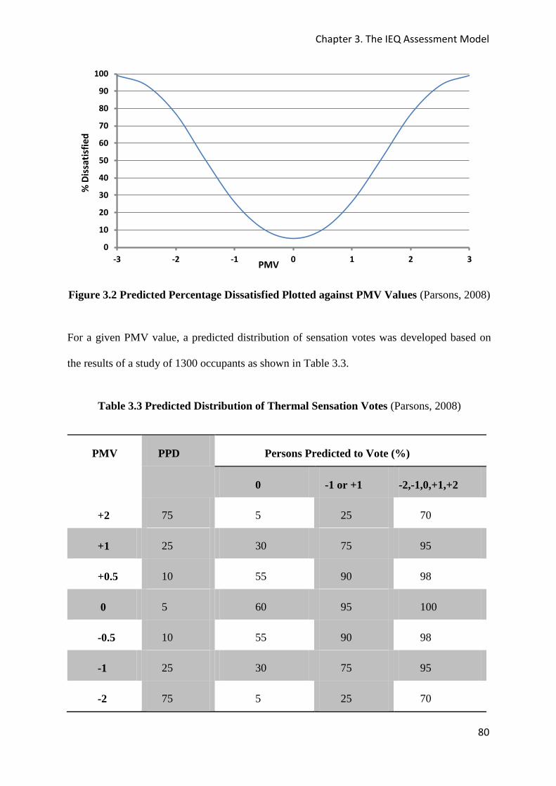
Chapter 3. The IEQ Assessment Model
80
Figure 3.2 Predicted Percentage Dissatisfied Plotted against PMV Values (Parsons, 2008)
For a given PMV value, a predicted distribution of sensation votes was developed based on
the results of a study of 1300 occupants as shown in Table 3.3.
Table 3.3 Predicted Distribution of Thermal Sensation Votes (Parsons, 2008)
PMV PPD Persons Predicted to Vote (%)
0 -1 or +1 -2,-1,0,+1,+2
+2 75 5 25 70
+1 25 30 75 95
+0.5 10 55 90 98
0 5 60 95 100
-0.5 10 55 90 98
-1 25 30 75 95
-2 75 5 25 70
0
10
20
30
40
50
60
70
80
90
100
-3 -2 -1 0 1 2 3
% D
issa
tisf
ied
PMV
Chapter 3. The IEQ Assessment Model
81
The PMV model relies on the absence of local discomfort factors such as draughts, vertical
temperature difference, cold surfaces, etc. Dissatisfaction with local discomfort factors can be
assessed separately using additional models, e.g. the draught models, PPD due to vertical
temperature differences, cold floors, etc. the percentage of people dissatisfied with draught is
given by the Draught Rating (DR) shown in equation 6.1.
経迎 噺 岫ぬね 伐 建銚岻岫懸 伐 ど┻どの岻待┻滞態 岫ど┻ぬば懸建通 髪 ぬ┻なね岻 惣┻ 層層
Discomfort caused by vertical air temperature difference is given as:
鶏経 噺 などど岫な 髪 結盤泰┻胎滞貸待┻腿泰滞ッ痛尼┸寧匪岻 惣┻ 層匝
Discomfort caused by warm or cold floors for people wearing light indoor shoes is estimated
by:
鶏経 噺 などど 伐 ひね 抜 結岫貸怠┻戴腿胎袋待┻怠怠腿痛肉貸待┻待待態泰痛肉鉄岻 惣┻ 層惣
Discomfort caused by radiant temperature asymmetry can also be calculated and the
methodology is found in the EN ISO7730 (2005) and is explained further in chapter 5.
For naturally ventilated offices a different assessment criteria will be adopted based on
adaptive thermal comfort models. A number of adaptive models have been developed and
many of these give similar predictions of comfort zones (Humphreys, 2000; Auliciems,
1981). In this thesis we shall adopt the Auliciems model which is based on the concept of
neutrality temperature, which is defined as the temperature at which most people feel
comfortable. Auliciems (1981) and other researchers found that the comfort temperature
inside the building is a function of temperatures prevailing outside the building, and we adopt

Chapter 3. The IEQ Assessment Model
82
this mode because it is based on a much more diverse set of building types. Using the model
the limits of thermal comfort categories in naturally ventilated buildings (see Figure 2.8,
Chapter 2) are bound by equations derived from the relationship below, for 5 < Toave < 35°C
for both the upper and the lower limits:
Tn value = 0.31*Toave + 17.6 ± Factor where Factor = 2.5 for Category I, 3.5 for category II
and 4.5 for category III (deDear and Brager, 2000)
It is therefore reasonable to assume that by adding more categories (for example category IV
has a factor of 5.5, and so on) we can produce the limiting equations for further categories
and therefore be able to plot percentage acceptance against operative temperatures as shown
in Appendix 5. Category I corresponds to 90% acceptance of the indoor environment and
category II and III correspond to 80% and 65% acceptance respectively, and so on (EN15251,
2006).
3.3.2 Development of the IAQ sub - index
The IAQ index is based on information obtained from European air quality guidelines
(Commission for European Communities, 1991; European Collaborative Action,
1992; NOHS, 2003; WHO, 2000). The performance requirements for ventilation and space
conditioning systems are presented in European standards (Meier et al, 2001; EN13779,
2006).
The quality of indoor air in an office building can be determined using any one of the three
indicators:
the concentrations of physical, chemical or biological pollutants in indoor air;
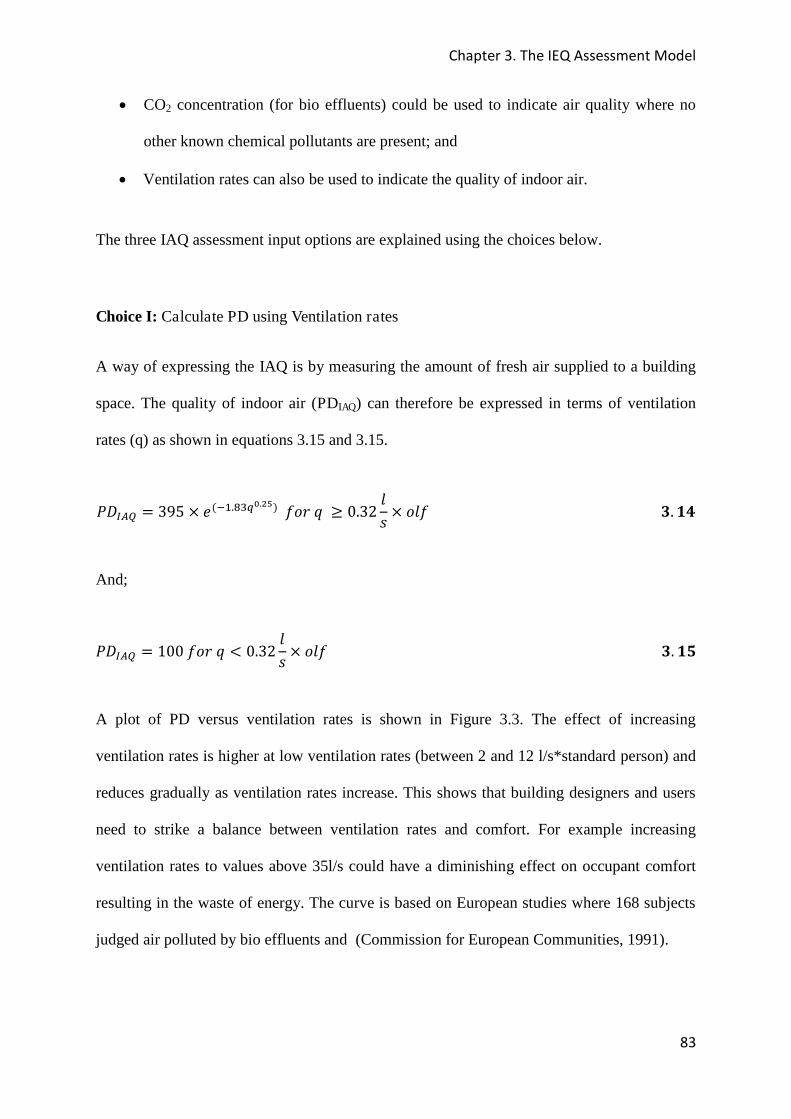
Chapter 3. The IEQ Assessment Model
83
CO2 concentration (for bio effluents) could be used to indicate air quality where no
other known chemical pollutants are present; and
Ventilation rates can also be used to indicate the quality of indoor air.
The three IAQ assessment input options are explained using the choices below.
Choice I: Calculate PD using Ventilation rates
A way of expressing the IAQ is by measuring the amount of fresh air supplied to a building
space. The quality of indoor air (PDIAQ) can therefore be expressed in terms of ventilation
rates (q) as shown in equations 3.15 and 3.15.
鶏経彫凋町 噺 ぬひの 抜 結岫貸怠┻腿戴槌轍┻鉄天岻 血剣堅 圏 半 ど┻ぬに 健嫌 抜 剣健血 惣┻ 層想
And;
鶏経彫凋町 噺 などど 血剣堅 圏 隼 ど┻ぬに 健嫌 抜 剣健血 惣┻ 層捜
A plot of PD versus ventilation rates is shown in Figure 3.3. The effect of increasing
ventilation rates is higher at low ventilation rates (between 2 and 12 l/s*standard person) and
reduces gradually as ventilation rates increase. This shows that building designers and users
need to strike a balance between ventilation rates and comfort. For example increasing
ventilation rates to values above 35l/s could have a diminishing effect on occupant comfort
resulting in the waste of energy. The curve is based on European studies where 168 subjects
judged air polluted by bio effluents and (Commission for European Communities, 1991).
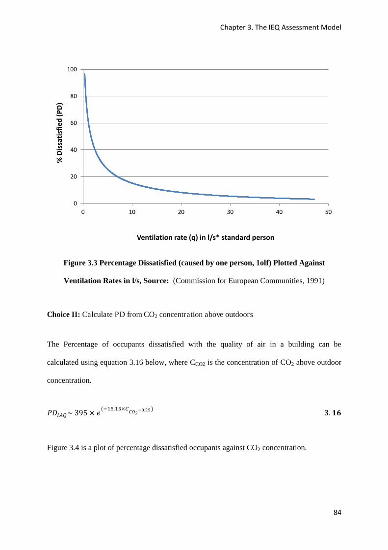
Chapter 3. The IEQ Assessment Model
84
Figure 3.3 Percentage Dissatisfied (caused by one person, 1olf) Plotted Against
Ventilation Rates in l/s, Source: (Commission for European Communities, 1991)
Choice II: Calculate PD from CO2 concentration above outdoors
The Percentage of occupants dissatisfied with the quality of air in a building can be
calculated using equation 3.16 below, where CCO2 is the concentration of CO2 above outdoor
concentration.
鶏経彫凋町b ぬひの 抜 結岫貸怠泰┻怠泰抜寵頓捺鉄貼轍┻鉄天岻 惣┻ 層掃
Figure 3.4 is a plot of percentage dissatisfied occupants against CO2 concentration.
0
20
40
60
80
100
0 10 20 30 40 50
% D
issa
tisf
ied
(P
D)
Ventilation rate (q) in l/s* standard person
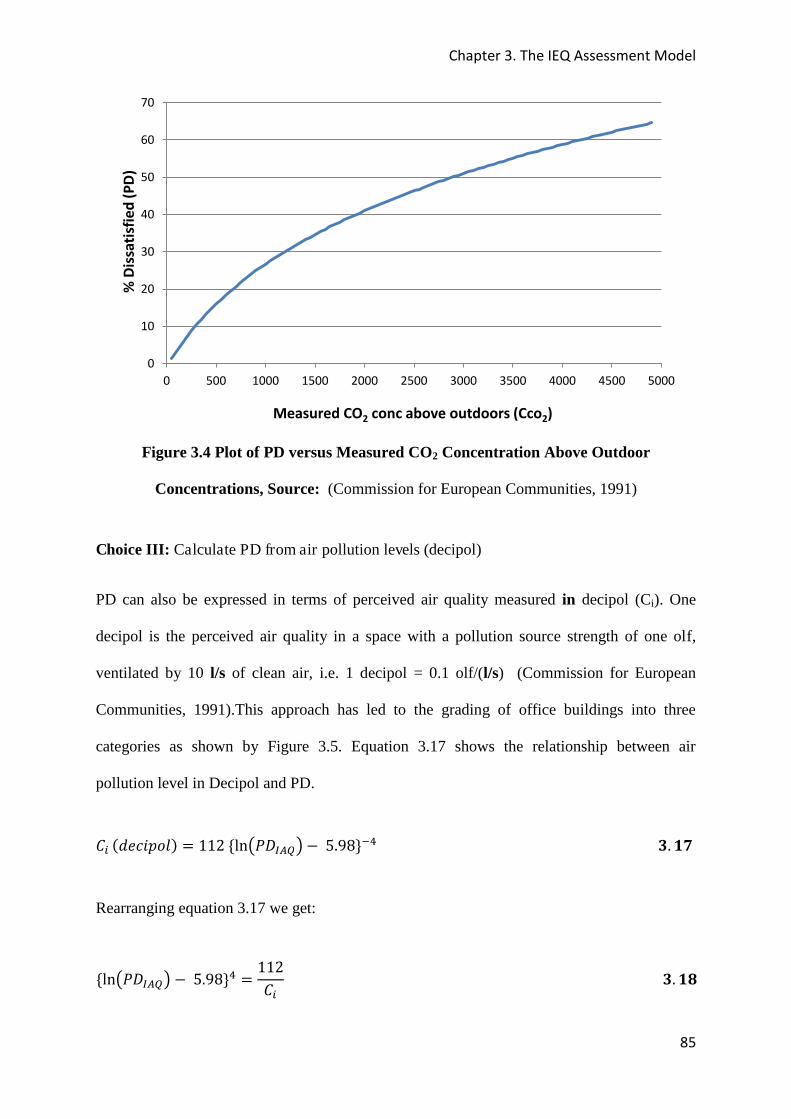
Chapter 3. The IEQ Assessment Model
85
Figure 3.4 Plot of PD versus Measured CO2 Concentration Above Outdoor
Concentrations, Source: (Commission for European Communities, 1991)
Choice III: Calculate PD from air pollution levels (decipol)
PD can also be expressed in terms of perceived air quality measured in decipol (Ci). One
decipol is the perceived air quality in a space with a pollution source strength of one olf,
ventilated by 10 l/s of clean air, i.e. 1 decipol = 0.1 olf/(l/s) (Commission for European
Communities, 1991).This approach has led to the grading of office buildings into three
categories as shown by Figure 3.5. Equation 3.17 shows the relationship between air
pollution level in Decipol and PD.
系沈 岫穴結潔件喧剣健岻 噺 ななに 岶 盤鶏経彫凋町匪 伐 の┻ひぱ岼貸替 惣┻ 層挿
Rearranging equation 3.17 we get:
岶 盤鶏経彫凋町匪 伐 の┻ひぱ岼替 噺 ななに系沈 惣┻ 層掻
0
10
20
30
40
50
60
70
0 500 1000 1500 2000 2500 3000 3500 4000 4500 5000
% D
issa
tisf
ied
(P
D)
Measured CO2 conc above outdoors (Cco2)
Chapter 3. The IEQ Assessment Model
86
岫鶏経彫凋町岻 ‒ の┻ひぱ 噺 磐ななに系沈 卑怠替 劇茎継軽┹ 岫鶏経彫凋町岻 噺 磐ななに系沈 卑怠替 髪 の┻ひぱ And finally:
鶏経彫凋町 噺 結岶貸峭 謬怠怠態寵日填 嶌袋泰┻苔腿岼 惣┻ 層操
Figure 3.5 Relationships Between Perceived Air Quality Expressed by the % of
Dissatisfied & Expressed in Decipol. The three indoor air quality levels,
categories A, B & C are shown. Source: (Commission for European
Communities, 1991)
Based on the percentage of persons dissatisfied with the aural environment, the IAQ index
(comfort) is therefore given as:
荊畦芸沈津鳥勅掴 噺 などど 伐 鶏経彫凋町 惣┻ 匝宋
0
10
20
30
40
50
60
70
0 2 4 6 8 10
% D
issa
tisf
ied
wit
h P
erc
eiv
ed
Air
Qu
ali
ty
Perceived Air Quality (Ci)
A
B
C
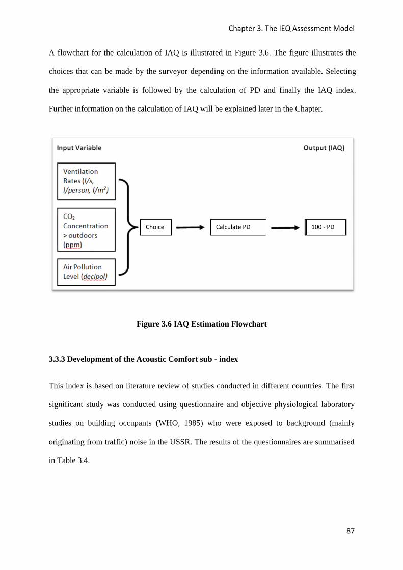
Chapter 3. The IEQ Assessment Model
87
A flowchart for the calculation of IAQ is illustrated in Figure 3.6. The figure illustrates the
choices that can be made by the surveyor depending on the information available. Selecting
the appropriate variable is followed by the calculation of PD and finally the IAQ index.
Further information on the calculation of IAQ will be explained later in the Chapter.
Figure 3.6 IAQ Estimation Flowchart
3.3.3 Development of the Acoustic Comfort sub - index
This index is based on literature review of studies conducted in different countries. The first
significant study was conducted using questionnaire and objective physiological laboratory
studies on building occupants (WHO, 1985) who were exposed to background (mainly
originating from traffic) noise in the USSR. The results of the questionnaires are summarised
in Table 3.4.
100 - PD Calculate PD Choice

Chapter 3. The IEQ Assessment Model
88
Table 3.4 Equivalent Sound Level vs. Number of Complaints, (WHO, 1985)
Equivalent sound level - dB(A) Number of Complaints in (%)
80 85
70 70
65 52.5
55 33
50 5
The second study which was carried by Kjellberg et al (1997) et al in Sweden investigated the
importance of frequency weighted sound level measurements on noise annoyance. It showed
a scenario where the rate of occupant annoyance increased with increasing sound level
(dBA). The study however produced a rather low correlation of 0.42 between noise levels and
rated annoyance. The third study carried out by Nilsson (2007) also developed a relationship
between A weighted sound pressure level and perceived annoyance in Sweden (Nilsson,
2007). By plotting A-weighted equivalent sound level against number of complaints for some
of these studies and including information from Bies et al (2009), we produce the curves in
Figure 3.7.
Figure 3.7 A-weighted Equivalent Sound Levels against % Complaints
0
10
20
30
40
50
60
70
80
90
100
0 20 40 60 80 100
% C
om
pla
ints
or
An
no
ye
d
Sound Level d(BA)
Kjellberg
Russian Studies
Bies, et al (lower)
Bies et al (higher)
Linear (Bies, et al
(lower))
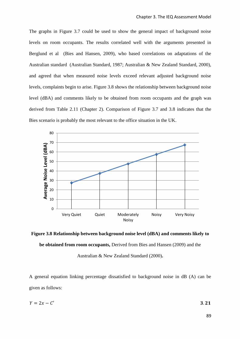
Chapter 3. The IEQ Assessment Model
89
The graphs in Figure 3.7 could be used to show the general impact of background noise
levels on room occupants. The results correlated well with the arguments presented in
Berglund et al (Bies and Hansen, 2009), who based correlations on adaptations of the
Australian standard (Australian Standard, 1987; Australian & New Zealand Standard, 2000),
and agreed that when measured noise levels exceed relevant adjusted background noise
levels, complaints begin to arise. Figure 3.8 shows the relationship between background noise
level (dBA) and comments likely to be obtained from room occupants and the graph was
derived from Table 2.11 (Chapter 2). Comparison of Figure 3.7 and 3.8 indicates that the
Bies scenario is probably the most relevant to the office situation in the UK.
Figure 3.8 Relationship between background noise level (dBA) and comments likely to
be obtained from room occupants, Derived from Bies and Hansen (2009) and the
Australian & New Zealand Standard (2000).
A general equation linking percentage dissatisfied to background noise in dB (A) can be
given as follows:
桁 噺 に捲 伐 系旺 惣┻ 匝層
0
10
20
30
40
50
60
70
80
Very Quiet Quiet Moderately
Noisy
Noisy Very Noisy
Av
era
ge
No
ise
Le
ve
l (d
BA
)

Chapter 3. The IEQ Assessment Model
90
Based on the arguments above we can formulate the following methodology:
1. Begin with a base level for acceptable noise in the space (we use target design values)
for this purpose;
2. Based on equation 3.21 above, the design value = 0.5*intercept on the x axis (C), i.e.
when Y=0, x=C/2, (taking a rather conservative assumption that a minimal number of
complaints will arise at that value);
3. For example assuming that complaints will only begin to rise in an office where the
acoustics design value is 35 dB(A), the equation becomes:
岫鶏経凋頂頂岻 噺 に岫決欠潔倦訣堅剣憲券穴 軽剣件嫌結 詣結懸結健 岫穴稽畦岻 伐 ぬの岻 惣┻ 匝匝
4. For an office with average background noise levels of 49 dBA, i.e 14 dBA above the
design value (35dBA), then PD = 28.
岫鶏経凋頂頂岻 噺 に盤畦潔建憲欠健聴墜通津鳥 牒追勅鎚鎚通追勅 挑勅塚勅鎮 伐 経結嫌件訣券聴墜通津鳥 椎追勅鎚鎚通追勅 鎮勅塚勅鎮 匪 惣┻ 匝惣
Y = % dissatisfied with noise and x = the background noise level in dB (A)
The Acoustic Comfort index is therefore estimated as:
畦潔潔沈津鳥勅掴 噺 などど 伐 鶏経凋頂頂 惣┻ 匝想
The Acoustic Comfort estimation Flowchart is shown in Figure 3.9
Figure 3.9 Acoustic Comfort Estimation Flowchart
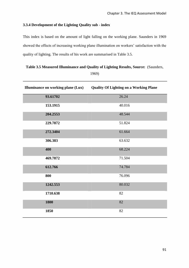
Chapter 3. The IEQ Assessment Model
91
3.3.4 Development of the Lighting Quality sub - index
This index is based on the amount of light falling on the working plane. Saunders in 1969
showed the effects of increasing working plane illumination on workers’ satisfaction with the
quality of lighting. The results of his work are summarised in Table 3.5.
Table 3.5 Measured Illuminance and Quality of Lighting Results, Source: (Saunders,
1969)
Illuminance on working plane (Lux) Quality Of Lighting on a Working Plane
93.61702 26.24
153.1915 40.016
204.2553 48.544
229.7872 51.824
272.3404 61.664
306.383 63.632
400 68.224
469.7872 71.504
612.766 74.784
800 76.096
1242.553 80.032
1710.638 82
1800 82
1850 82
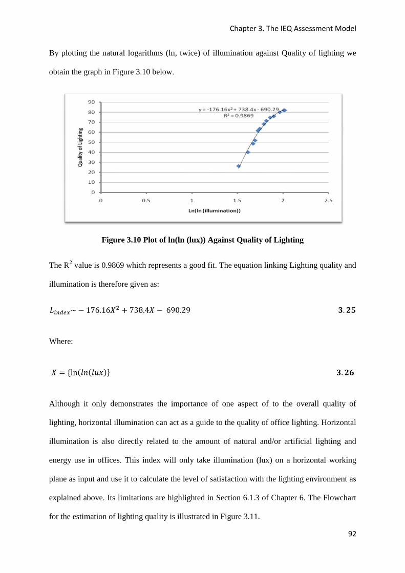
Chapter 3. The IEQ Assessment Model
92
By plotting the natural logarithms (ln, twice) of illumination against Quality of lighting we
obtain the graph in Figure 3.10 below.
Figure 3.10 Plot of ln(ln (lux)) Against Quality of Lighting
The R2 value is 0.9869 which represents a good fit. The equation linking Lighting quality and
ill umination is therefore given as:
詣沈津鳥勅掴b伐 なばは┻なは隙態 髪 ばぬぱ┻ね隙 伐 はひど┻にひ 惣┻ 匝捜
Where:
隙 噺 岶 岫健券岫健憲捲岻岼 惣┻ 匝掃
Although it only demonstrates the importance of one aspect of to the overall quality of
lighting, horizontal illumination can act as a guide to the quality of office lighting. Horizontal
illumination is also directly related to the amount of natural and/or artificial lighting and
energy use in offices. This index will only take illumination (lux) on a horizontal working
plane as input and use it to calculate the level of satisfaction with the lighting environment as
explained above. Its limitations are highlighted in Section 6.1.3 of Chapter 6. The Flowchart
for the estimation of lighting quality is illustrated in Figure 3.11.

Chapter 3. The IEQ Assessment Model
93
Figure 3.11 Lighting Comfort Estimation Flowchart
3.3.5 Developing the Perceived IEQ index and the Weightings
Very little research has been attributed to the development of single index based IEQ tools
because it is difficult to establish how individual factors contribute to overall IEQ. In this
thesis the IEQ model relies on the establishment of a linear relationship between perceived
IEQ and contributing factors as described in the Chiang and Lai IEQ model (2002). We adopt
the linear approach as a credible indicator of the indoor environment and accept that the
impact of the contributing factors, i.e. the sub-indices or sub-indicators represent sanitary risk
factors to the occupants (Hult, 1998). For example, a thermal comfort score of 50% PD
represents a certain level of risk of causing discomfort to the occupant. We therefore assume
that a cumulative effect of risk factors (contributing parameters) could impact on the
occupant’s perception of the indoor environment. We also accept that a reduction in risk
means a better environment for occupants.
Within each sub-indicator, there are specific metrics that can be utilized in determining an
acceptable quality of an indoor environment based on existing knowledge as explained
earlier. However the true impacts of each of the contributing factors on perceived IEQ are not
yet fully understood and more research is needed in this area. In this study we will take full
advantage of the predictive nature of empirical regression models simply because they are
derived from subjective measurements.

Chapter 3. The IEQ Assessment Model
94
The model is not based on causal relations, and does not claim that a causal relation exists
between the index and its contributors, but it takes advantage of the predictive ability of
correlational relationships. As such, it should be used with caution. The Overall IEQ index
(IEQindex) is expressed as a function of thermal comfort, IAQ, acoustic comfort and lighting
quality as shown in the expressions 3.27 – 3.30 below.
荊継芸沈津鳥勅掴 噺 枌 岫劇潔沈津鳥勅掴 ┸ 荊畦芸沈津鳥勅掴 ┸ 畦系潔沈津鳥勅掴 ┸ 詣沈津鳥勅掴 ┸ ┼ ┸ ┼┼ ┸┼┼┼ ┻ 岻 惣┻ 匝挿
荊継芸沈津鳥勅掴 噺 布紅沈鯨荊沈津沈退待 惣┻ 匝掻
荊継芸沈津鳥勅掴 噺 紅怠 抜 劇潔沈津鳥勅掴 髪 紅態 抜 荊畦芸沈津鳥勅掴 髪 紅戴 抜 畦系潔沈津鳥勅掴 髪 紅替 抜 詣沈津鳥勅掴 髪橋 ┸ ┻ ┻ 惣┻ 匝操
Where く1 – く4 are the weighting coefficients that can be derived from regression results
obtained from questionnaire data or by other means and SI is the sub index.
Several methods that can be used for estimating the weightings of each of the contributors are
available in literature. The two most important are the use of the Analytical Hierarchy
Process (AHP) and the fitting of results of subjective evaluation to regression models. The
latter process and methodology will be explained in Chapter 4. Chiang and Lai (2002)
derived the weightings associated with five main factors contributing to perceived IEQ (くi)
using the AHP and tested the model in built buildings in Taiwan. The Analytic Hierarchy
Process (AHP) is a mathematical decision-making technique that provides an effective means
of dealing with tasks that need complex decision-making techniques.
The process was first developed by Saaty (1979) and is now widely applied in science and
engineering decision making processes. More information on the AHP in science and
engineering can be found in Jurgen et al (20101). Chiang and Lai (2002) involved consulting
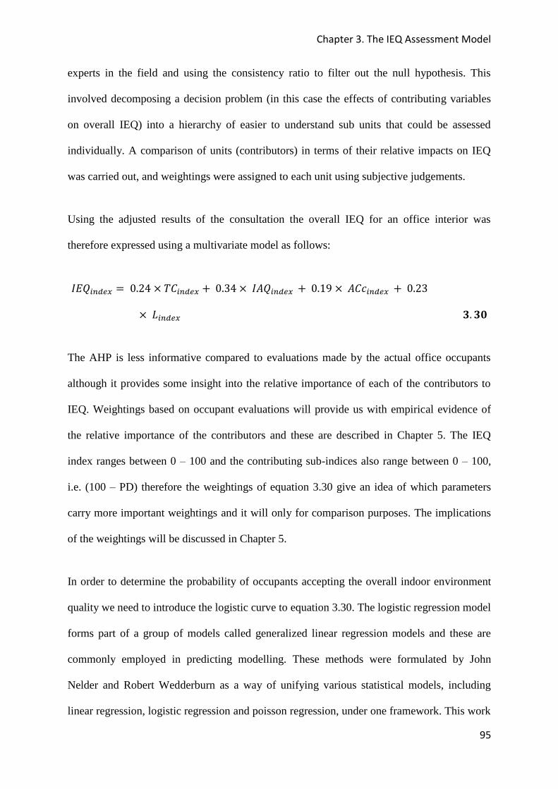
Chapter 3. The IEQ Assessment Model
95
experts in the field and using the consistency ratio to filter out the null hypothesis. This
involved decomposing a decision problem (in this case the effects of contributing variables
on overall IEQ) into a hierarchy of easier to understand sub units that could be assessed
individually. A comparison of units (contributors) in terms of their relative impacts on IEQ
was carried out, and weightings were assigned to each unit using subjective judgements.
Using the adjusted results of the consultation the overall IEQ for an office interior was
therefore expressed using a multivariate model as follows:
荊継芸沈津鳥勅掴 噺 ど┻にね 抜 劇系沈津鳥勅掴 髪 ど┻ぬね 抜 荊畦芸沈津鳥勅掴 髪 ど┻なひ 抜 畦系潔沈津鳥勅掴 髪 ど┻にぬ抜 詣沈津鳥勅掴 惣┻ 惣宋
The AHP is less informative compared to evaluations made by the actual office occupants
although it provides some insight into the relative importance of each of the contributors to
IEQ. Weightings based on occupant evaluations will provide us with empirical evidence of
the relative importance of the contributors and these are described in Chapter 5. The IEQ
index ranges between 0 – 100 and the contributing sub-indices also range between 0 – 100,
i.e. (100 – PD) therefore the weightings of equation 3.30 give an idea of which parameters
carry more important weightings and it will only for comparison purposes. The implications
of the weightings will be discussed in Chapter 5.
In order to determine the probability of occupants accepting the overall indoor environment
quality we need to introduce the logistic curve to equation 3.30. The logistic regression model
forms part of a group of models called generalized linear regression models and these are
commonly employed in predicting modelling. These methods were formulated by John
Nelder and Robert Wedderburn as a way of unifying various statistical models, including
linear regression, logistic regression and poisson regression, under one framework. This work

Chapter 3. The IEQ Assessment Model
96
can be found in the textbook, Generalized Linear Models by Nelder and McCullagh (1989).
These approaches have been used extensively in statistical analysis, however most models
give strange results especially in cases where the dependent variable is an event. Since the
probability of an event must lie between 0 and 1, it is impractical to model probabilities
especially with linear regression techniques because linear regression models allow the
dependent variable to take values greater than 1 or less than 0 (Merton, 1968) in some cases.
The solution to this problem would be to generalize the linear model by coupling it with a
sensible distribution for the dependent variable. This approach is called Logistic Regression
Modelling and it makes use of several predictor variables that may be either numerical or
categorical. Binary logistic regression has been found to be most useful when one wants to
model the event probability for a categorical response variable with two outcomes (Merton,
1968). It could also be employed in situations where predictions are difficult or impossible to
make, where tails fit badly and where variance cannot be constant (Wong et al, 2007).
Logistic regression (or logit) has been extensively employed in social research, medicine,
engineering, agriculture (Hahn and Soyer, 2005) and more specifically in modelling of the
indoor environment by Wong et al (2007). Wong used the model to predict the probability of
acceptance of IEQ in offices in Hong Kong by fitting questionnaire data to a logistic curve.
The Logistic Regression Model can be explained as follows:
Let us begin by considering the existence of an unobserved continuous variable, Z, which can
be thought of as the "propensity towards" the acceptability of IEQ and in this thesis, Z =
IEQindex. In such cases larger values of Z correspond to greater probabilities of acceptance of
the indoor environment while lower values of Z correspond to lower probabilities of
acceptance of the IEQ. The logistic function and its inverse link are illustrated by equations
shown below.
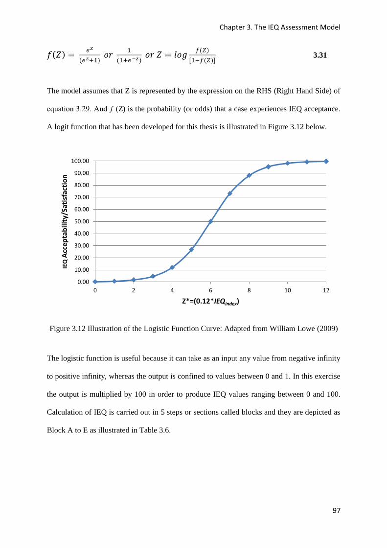
Chapter 3. The IEQ Assessment Model
97
血岫傑岻 噺 勅年岫勅年袋怠岻 剣堅 怠岫怠袋勅貼年岻 剣堅 傑 噺 健剣訣 捗岫跳岻岷怠貸捗岫跳岻峅 3.31
The model assumes that Z is represented by the expression on the RHS (Right Hand Side) of
equation 3.29. And ƒ (Z) is the probability (or odds) that a case experiences IEQ acceptance.
A logit function that has been developed for this thesis is illustrated in Figure 3.12 below.
Figure 3.12 Illustration of the Logistic Function Curve: Adapted from William Lowe (2009)
The logistic function is useful because it can take as an input any value from negative infinity
to positive infinity, whereas the output is confined to values between 0 and 1. In this exercise
the output is multiplied by 100 in order to produce IEQ values ranging between 0 and 100.
Calculation of IEQ is carried out in 5 steps or sections called blocks and they are depicted as
Block A to E as illustrated in Table 3.6.
0.00
10.00
20.00
30.00
40.00
50.00
60.00
70.00
80.00
90.00
100.00
0 2 4 6 8 10 12
IEQ
Acc
ep
tab
ilit
y/S
ati
sfa
ctio
n
Z*=(0.12*IEQindex)
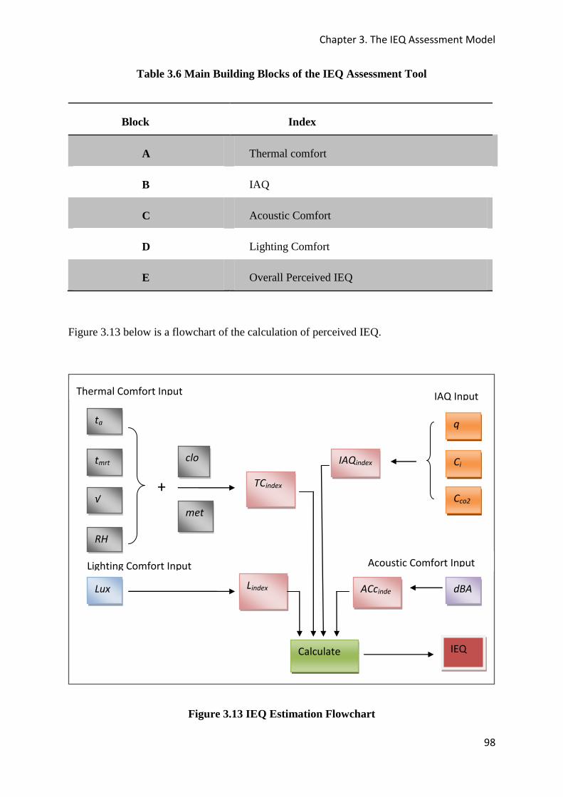
Chapter 3. The IEQ Assessment Model
98
Table 3.6 Main Building Blocks of the IEQ Assessment Tool
Block Index
A Thermal comfort
B IAQ
C Acoustic Comfort
D Lighting Comfort
E Overall Perceived IEQ
Figure 3.13 below is a flowchart of the calculation of perceived IEQ.
Figure 3.13 IEQ Estimation Flowchart
ta
tmrt
я
RH
+
clo
met
TCindex
IAQindex
Lindex ACcinde
x
q
Ci
Cco2
dBA Lux
Calculate IEQ
Thermal Comfort Input IAQ Input
Lighting Comfort Input Acoustic Comfort Input
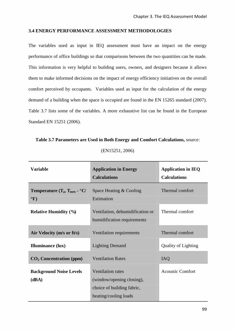
Chapter 3. The IEQ Assessment Model
99
3.4 ENERGY PERFORMANCE ASSESSMENT METHODOLOGIES
The variables used as input in IEQ assessment must have an impact on the energy
performance of office buildings so that comparisons between the two quantities can be made.
This information is very helpful to building users, owners, and designers because it allows
them to make informed decisions on the impact of energy efficiency initiatives on the overall
comfort perceived by occupants. Variables used as input for the calculation of the energy
demand of a building when the space is occupied are found in the EN 15265 standard (2007).
Table 3.7 lists some of the variables. A more exhaustive list can be found in the European
Standard EN 15251 (2006).
Table 3.7 Parameters are Used in Both Energy and Comfort Calculations, source:
(EN15251, 2006)
Variable Application in Energy
Calculations
Application in IEQ
Calculations
Temperature (Ta, Tmrt, - °C/
°F)
Space Heating & Cooling
Estimation
Thermal comfort
Relative Humidity (%) Ventilation, dehumidification or
humidification requirements
Thermal comfort
Air Velocity (m/s or ft/s) Ventilation requirements Thermal comfort
Illuminance (lux) Lighting Demand Quality of Lighting
CO2 Concentration (ppm) Ventilation Rates IAQ
Background Noise Levels
(dBA)
Ventilation rates
(window/opening closing),
choice of building fabric,
heating/cooling loads
Acoustic Comfort
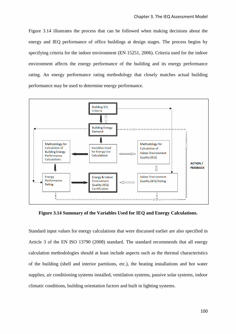
Chapter 3. The IEQ Assessment Model
100
Figure 3.14 illustrates the process that can be followed when making decisions about the
energy and IEQ performance of office buildings at design stages. The process begins by
specifying criteria for the indoor environment (EN 15251, 2006). Criteria used for the indoor
environment affects the energy performance of the building and its energy performance
rating. An energy performance rating methodology that closely matches actual building
performance may be used to determine energy performance.
Figure 3.14 Summary of the Variables Used for IEQ and Energy Calculations.
Standard input values for energy calculations that were discussed earlier are also specified in
Article 3 of the EN ISO 13790 (2008) standard. The standard recommends that all energy
calculation methodologies should at least include aspects such as the thermal characteristics
of the building (shell and interior partitions, etc.), the heating installations and hot water
supplies, air conditioning systems installed, ventilation systems, passive solar systems, indoor
climatic conditions, building orientation factors and built in lighting systems.
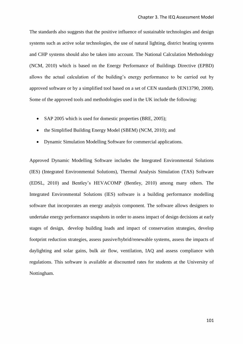
Chapter 3. The IEQ Assessment Model
101
The standards also suggests that the positive influence of sustainable technologies and design
systems such as active solar technologies, the use of natural lighting, district heating systems
and CHP systems should also be taken into account. The National Calculation Methodology
(NCM, 2010) which is based on the Energy Performance of Buildings Directive (EPBD)
allows the actual calculation of the building’s energy performance to be carried out by
approved software or by a simplified tool based on a set of CEN standards (EN13790, 2008).
Some of the approved tools and methodologies used in the UK include the following:
SAP 2005 which is used for domestic properties (BRE, 2005);
the Simplified Building Energy Model (SBEM) (NCM, 2010); and
Dynamic Simulation Modelling Software for commercial applications.
Approved Dynamic Modelling Software includes the Integrated Environmental Solutions
(IES) (Integrated Environmental Solutions), Thermal Analysis Simulation (TAS) Software
(EDSL, 2010) and Bentley’s HEVACOMP (Bentley, 2010) among many others. The
Integrated Environmental Solutions (IES) software is a building performance modelling
software that incorporates an energy analysis component. The software allows designers to
undertake energy performance snapshots in order to assess impact of design decisions at early
stages of design, develop building loads and impact of conservation strategies, develop
footprint reduction strategies, assess passive/hybrid/renewable systems, assess the impacts of
daylighting and solar gains, bulk air flow, ventilation, IAQ and assess compliance with
regulations. This software is available at discounted rates for students at the University of
Nottingham.

Chapter 3. The IEQ Assessment Model
102
The Thermal Analysis Simulation (TAS) Software is capable of performing dynamic thermal
simulation of buildings including the ability to predict energy consumption, CO2 emissions,
operation costs and occupant comfort (thermal comfort). The software can be used to
calculate heating and cooling loads, design natural or passive ventilation systems, evaluate
ventilation regimes, simulations, daylighting calculations and to check compliance with
legislation. The software is available free at selected computers within the University of
Nottingham.
Bentley’s HEVACOMP software is a leading tool in building services design and CAD
software that uses industry standard calculation procedures such as CIBSE, ASHRAE, British
Standards or IEE as applicable. The software has found applications in Mechanical design for
Load calculations, Pipe & duct sizing and Mechanical CAD. Both 2-D & 3-D CAD drawings
can be produced. Energy calculations based on the Energy Plus analysis engine can be carried
out to examine room heat losses and gains, summer overheating, peak design months,
overheating frequency, building energy and therefore equipment sizing. CFD simulations for
heat flow (T°C), air movement (ventilation) and particulate concentrations (pollution)
including electrical design conforming to the requirements of IEE 16th Edition wiring
regulations, Lighting systems design and electrical CAD can also be carried out. This
software was also available free for purposes of this research at the University of Nottingham
and at Hoare Lea & Partners.
The energy performance of office buildings is highlighted using Energy Performance
Certificates (EPCs) which can be produced using software such as explained above. EPCs are
used to grade buildings on a scale of A to G with A being the most efficient and G the least.
Figure 3.15 shows a typical building rated at Grade D with a potential to rate Grade C. In
commercial buildings asset certificates measure the intrinsic energy performance of the

Chapter 3. The IEQ Assessment Model
103
building based on its design while operating certificates measure how the building is
managed and how it actually performs. The certificates are renewed annually and displayed
in public buildings. EPCs are based on the SAP 2005 ratings and SBEM (BRE, 2005).
Figure 3.15 Energy Performance Certificate Showing a D Rated Domestic Building:
copied from: (Directgov, 2011).
3.5 THE IEQAT
Based on the findings of the previous sections of this Chapter that included the identification
of factors influencing IEQ and their respective variables, the development of sub indices, the
use of weighting coefficients developed by Chiang et al to develop the IEQ index and a list of
appropriate programming software the IEQAT could be assembled and used as shown in the
example sheets (data entry and assessment sheets). The IEQAT consists of numbered data
entry sheets where information relevant to building assessment model is entered. It also
consists of assessment sheets that summarise IEQ performance of buildings. A general
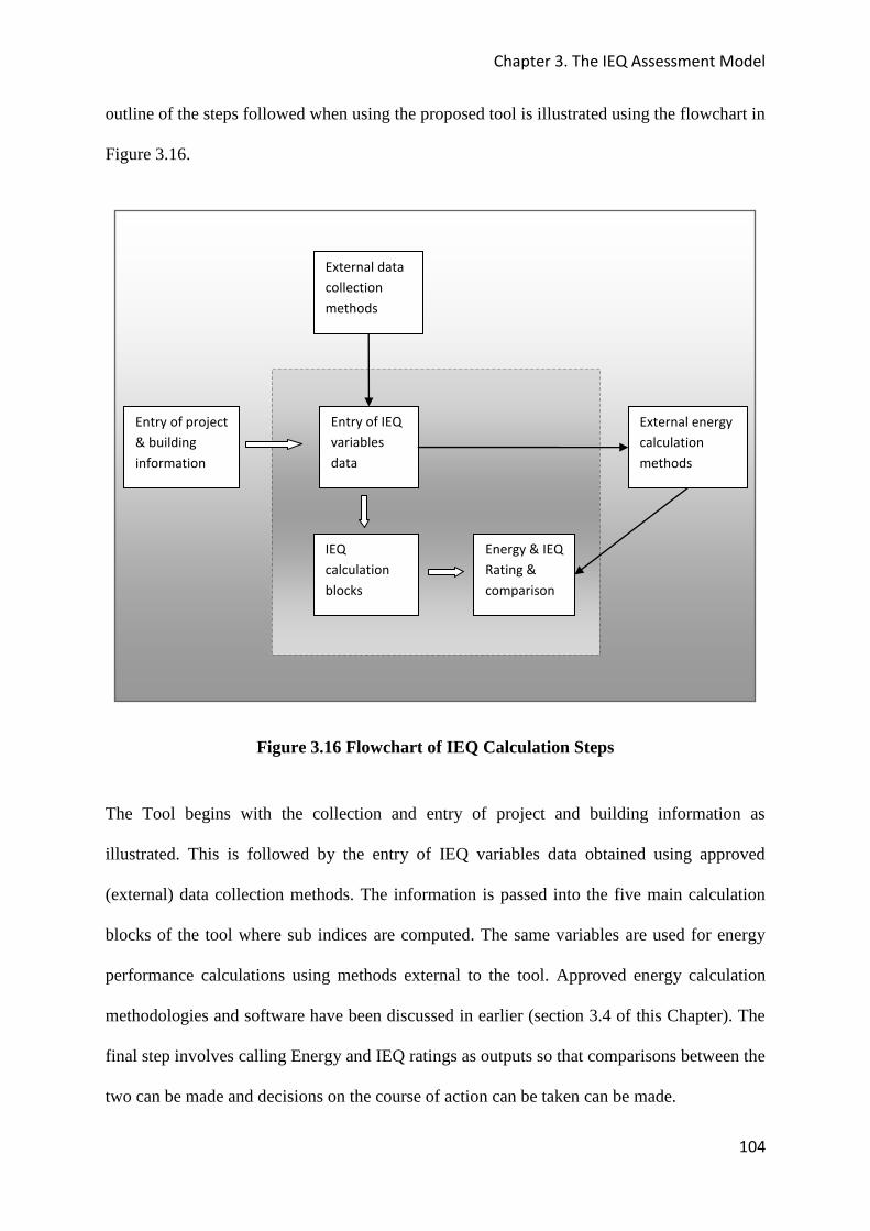
Chapter 3. The IEQ Assessment Model
104
outline of the steps followed when using the proposed tool is illustrated using the flowchart in
Figure 3.16.
Figure 3.16 Flowchart of IEQ Calculation Steps
The Tool begins with the collection and entry of project and building information as
illustrated. This is followed by the entry of IEQ variables data obtained using approved
(external) data collection methods. The information is passed into the five main calculation
blocks of the tool where sub indices are computed. The same variables are used for energy
performance calculations using methods external to the tool. Approved energy calculation
methodologies and software have been discussed in earlier (section 3.4 of this Chapter). The
final step involves calling Energy and IEQ ratings as outputs so that comparisons between the
two can be made and decisions on the course of action can be taken can be made.
Entry of project
& building
information
External data
collection
methods
External energy
calculation
methods
Entry of IEQ
variables
data
IEQ
calculation
blocks
Energy & IEQ
Rating &
comparison
Chapter 3. The IEQ Assessment Model
105
3.5.1. Data Input
The IEQ tool has the ability to capture user and project data using a data entry sheets or
windows (for computer based programs, see screenshot). The main sheet where the user
makes the first input is shown in Figure 3.17.
Figure 3.17 Data Entry Sheet 1/1– Project and Building Data
The first data entry sheet allows the assessor to input information which is important for
identifying projects. The information required here consists of basic information necessary to
carry out an assessment. The second set of information required by this sheet is the building
data. In this section information that identifies the building is entered. Most of the
information requested is self explanatory and fairly easy to comprehend by qualified
assessors.

Chapter 3. The IEQ Assessment Model
106
For computer based products the creation of IEQ projects using the normal windows or MAC
procedures is expected. As in most cases the program may ask the user to identify themselves
by way of logins and ask them to either create new projects or work on existing ones. The
type of office refers to whether the office is an open plan, cubicle, or a mixture of the two and
also requires the user to specify the type of HVAC system present. There are four generic
types of office in the UK and they are listed below.
Naturally Ventilated Cellular offices are relatively simple and small offices that are mostly
converted from residential accommodation. They have typical floor spaces ranging from 100
to 3000m2. Local comfort controls such as local light switches and heating controls are
common practice. A different thermal comfort assessment criterion is used for naturally
ventilated offices where occupants are free to adapt their clothing levels and other local
comfort parameters as explained in Chapter 2, section 2.7.2.
Naturally Ventilated Open Plan offices are largely open plan but some may have cellular
spaces. Typically they range from 500 to 4000m2 in floor area and they are sometimes built
in converted industrial space or specially designated areas. Equipment use is usually more
intense than in cellular offices as frequent switching on and off of equipment is carried out to
satisfy a larger group of occupants.
Standard Air Conditioned offices are largely purpose built with floor areas ranging from
2000 to 8000m2. The benchmarks are usually based on Variable Air Volume (VAV) air
conditioning systems.
Prestige Air Conditioned offices are usually associated with regional head offices and
administrative centres with typical floor spaces ranging from 4000 to 20 000m2. The offices
are usually built or refurbished to very high standards with excellent BMS. Air conditioning

Chapter 3. The IEQ Assessment Model
107
is usually provided for specialist areas such as server rooms and even in parking and leisure
areas. In some cases Personalised Ventilation Systems (PVS) are installed to provide
individualised comfort (BRECSU, 2000).
Mixed Mode offices are those that combine both passive natural ventilation and mechanical
ventilation and cooling in buildings that may otherwise have been fully air conditioned. In
most cases in the UK mechanical ventilation may be used only during the cooling season.
More information on the benchmarks for all office types can be found in the Energy use in
Offices Guide 19 (BRECSU, 2000).
The number of floors, floor number and floor area are self explanatory and they are important
aspects that help provide clues about energy use and comfort. Floor area and occupancy
levels give the population density within the office (number of occupants per unit area) and
these in turn affect the selection and performance of HVAC systems.
The section of the office refers to the part of the space under investigation and includes
sections, zones, blocks, etc. The location and climate requires the user to enter the actual
location and climatic zone for purposes of estimating the microclimatic conditions that exist
in and around the building. Nowadays most software use databases containing up to date
weather and pollution data. The date the office was built refers to the actual date of
completion and if any renovations were made then they need to be stated.
For buildings still to be built or those under construction an expected date of completion may
be entered. Figure 3.18 is the second part of the first data entry sheet and it requires the user
to enter a general description of the building in the words of the assessor.

Chapter 3. The IEQ Assessment Model
108
Figure 3.18 Data Entry Sheet 2 / 1 – Project and Building Data
The second step involves the selection of the type of data to be used as input for calculating
IEQ. This is especially important since the data origins could have different accuracy and
reliability implications (Fairfax County Department of Systems Management for Human
Services, 2003). Input data selection, the source of the data and the collection interval is
summarised in the tool data input sheet shown in Figure 3.19. The “type” of data especially
refers to its source or origin i.e. measured, calculated, design and questionnaire data as
explained below. This section also requires the user to draw or upload floor plans.
Figure 3.19 Data Entry Sheet 2
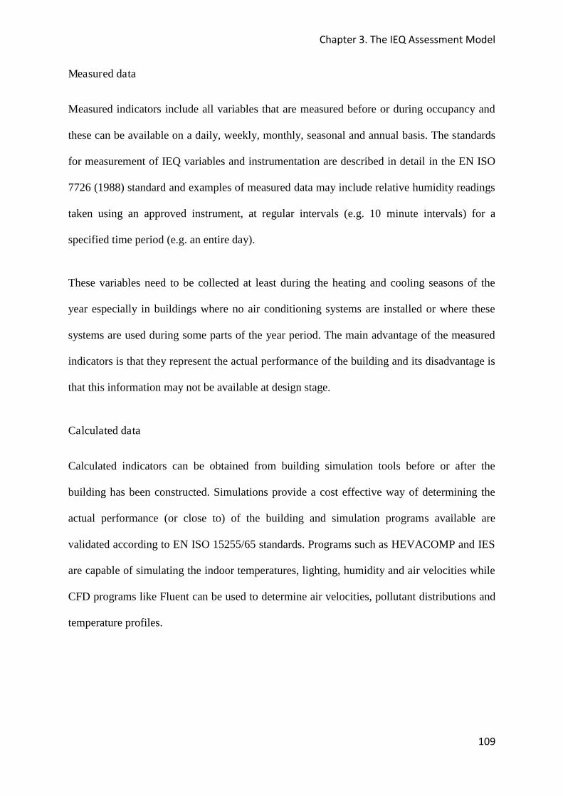
Chapter 3. The IEQ Assessment Model
109
Measured data
Measured indicators include all variables that are measured before or during occupancy and
these can be available on a daily, weekly, monthly, seasonal and annual basis. The standards
for measurement of IEQ variables and instrumentation are described in detail in the EN ISO
7726 (1988) standard and examples of measured data may include relative humidity readings
taken using an approved instrument, at regular intervals (e.g. 10 minute intervals) for a
specified time period (e.g. an entire day).
These variables need to be collected at least during the heating and cooling seasons of the
year especially in buildings where no air conditioning systems are installed or where these
systems are used during some parts of the year period. The main advantage of the measured
indicators is that they represent the actual performance of the building and its disadvantage is
that this information may not be available at design stage.
Calculated data
Calculated indicators can be obtained from building simulation tools before or after the
building has been constructed. Simulations provide a cost effective way of determining the
actual performance (or close to) of the building and simulation programs available are
validated according to EN ISO 15255/65 standards. Programs such as HEVACOMP and IES
are capable of simulating the indoor temperatures, lighting, humidity and air velocities while
CFD programs like Fluent can be used to determine air velocities, pollutant distributions and
temperature profiles.

Chapter 3. The IEQ Assessment Model
110
Design data
The use of design indicators to indicate the quality of the indoor environment is one of the
first steps in the design of any office. Categories presented later in this chapter are generally
used to classify buildings. Recommended design values for temperature, humidity,
ventilation rates, illumination, background noise, etc have already been presented in the
recommended operation of office buildings in Chapter 2. The main advantage of using design
indicators is that the IEQ of the building can be determined before construction and
adjustments to the HVAC systems can be made at an early stage. The main disadvantage is
that buildings may not perform to intended standards.
Questionnaire (survey) Data
The use of subjective evaluation to assess building performance is probably the best option as
it gives the actual information on how occupants feel inside the building. Questionnaire data
may include data collected through preset questions that are handed to office occupants
electronically, by interviewing or by delivering hard copies and collecting those after the
occupants have expressed their opinion of the indoor environment. Questionnaires are
relatively easy and cheap to administer. However the main disadvantage is that
questionnaires can only be used for post occupancy evaluation. This next step involves the
selection of data source files (Figure 3.18). Data can either be entered manually for single
entry calculations or via file upload. Uploading data allows multiple values to be entered for
example data collected over a period of time could be uploaded instantly and IEQ can be
calculated for that period. In some cases data could be received from the BMS allowing
calculations to be carried out instantly (real time monitoring of IEQ). Entered data can be
displayed in the display area (not shown) and amended as required. Examples of files are
shown in Tables 3.8 and 3.9.

Chapter 3. The IEQ Assessment Model
111
Table 3.8 shows data that has been collected on a monthly basis for a year and Table 3.9
shows data that has been collected hourly for a 12 hour day. This data could also show
average values, for example Table 3.14 could show mean monthly values of variables which
have been collected on a second by second basis, hourly, daily or weekly basis. This
information shows the flexibility of the input data for tool and hence the output data
expected.
Table 3.8 Example of an Annual File with Data Collected Monthly
Table 3.9 Example of a 12 hour Day File with Data Collected Every Hour
Month Ta (°C) Tmrt (°C) RH (%) V (m/s) Clo Met Lux IAQ choiceAcosutics (dBA)
January
February
March
April
May
June
July
August
September
October
November
December
Hour Ta (°C) Tmrt (°C) RH (%) V (m/s) Clo Met Lux IAQ choice Acosutics (dBA)
1
2
3
4
5
6
7
8
9
10
11
12
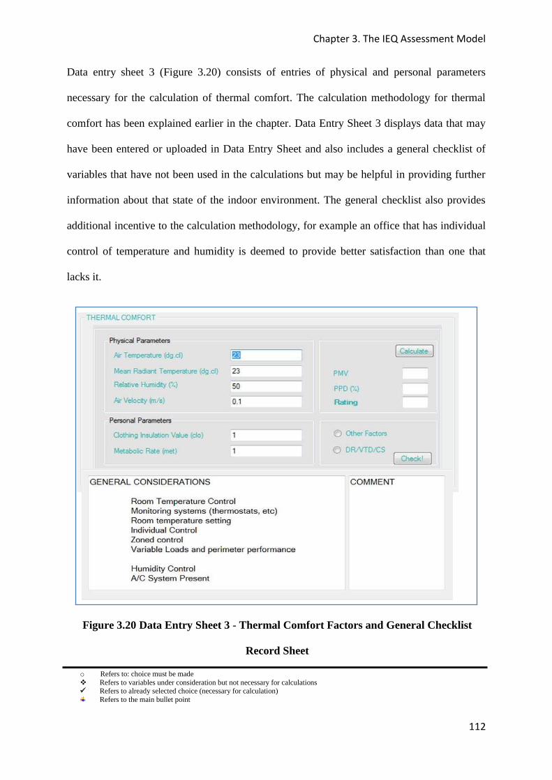
Chapter 3. The IEQ Assessment Model
112
Data entry sheet 3 (Figure 3.20) consists of entries of physical and personal parameters
necessary for the calculation of thermal comfort. The calculation methodology for thermal
comfort has been explained earlier in the chapter. Data Entry Sheet 3 displays data that may
have been entered or uploaded in Data Entry Sheet and also includes a general checklist of
variables that have not been used in the calculations but may be helpful in providing further
information about that state of the indoor environment. The general checklist also provides
additional incentive to the calculation methodology, for example an office that has individual
control of temperature and humidity is deemed to provide better satisfaction than one that
lacks it.
Figure 3.20 Data Entry Sheet 3 - Thermal Comfort Factors and General Checklist
Record Sheet
o Refers to: choice must be made Refers to variables under consideration but not necessary for calculations Refers to already selected choice (necessary for calculation)
Refers to the main bullet point
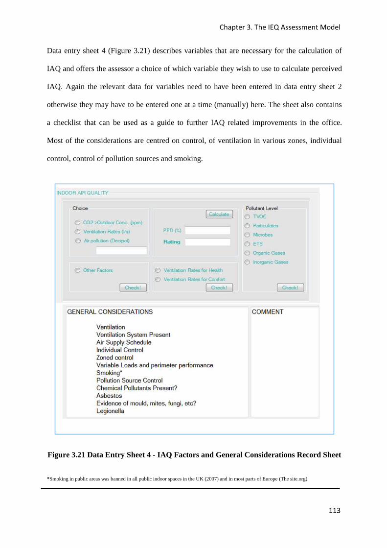
Chapter 3. The IEQ Assessment Model
113
Data entry sheet 4 (Figure 3.21) describes variables that are necessary for the calculation of
IAQ and offers the assessor a choice of which variable they wish to use to calculate perceived
IAQ. Again the relevant data for variables need to have been entered in data entry sheet 2
otherwise they may have to be entered one at a time (manually) here. The sheet also contains
a checklist that can be used as a guide to further IAQ related improvements in the office.
Most of the considerations are centred on control, of ventilation in various zones, individual
control, control of pollution sources and smoking.
Figure 3.21 Data Entry Sheet 4 - IAQ Factors and General Considerations Record Sheet
*Smoking in public areas was banned in all public indoor spaces in the UK (2007) and in most parts of Europe (The site.org)
Chapter 3. The IEQ Assessment Model
114
Data entry sheet 5 (Figure 3.22) displays the variable that is used in this tool to estimate
perceived acoustic comfort and the other considerations that need to be made to ensure an
acceptable acoustic environment for occupants. Background noise level (dBA) is the only
variable used in this sheet and its use in the estimation of acoustic comfort is also presented
later in the chapter.
The general considerations checklist includes the analysis of type and intensity of equipment,
people and outdoor noise. This can be observed directly by the assessor during the
assessment exercise. This process is referred to as critical listening and it is a cheap, easy but
effective method of identifying annoying background noise. Sound insulation properties of
elements of the building fabric such as walls, floors, openings and the reverberation times of
sound can be obtained from building construction data.
The information can help identify problem areas and hence help determine what sound
related improvements need to be made.
Figure 3.22 Data Entry Sheet 5 – Acoustic Comfort Factors and General Considerations
Record Sheet
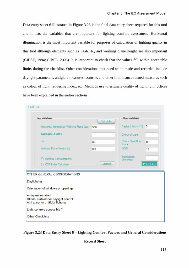
Chapter 3. The IEQ Assessment Model
115
Data entry sheet 6 illustrated in Figure 3.23 is the final data entry sheet required for this tool
and it lists the variables that are important for lighting comfort assessment. Horizontal
illumination is the most important variable for purposes of calculation of lighting quality in
this tool although elements such as UGR, Ra and working plane height are also important
(CIBSE, 1994; CIBSE, 2006). It is important to check that the values fall within acceptable
limits during the checklist. Other considerations that need to be made and recorded include
daylight parameters, antiglare measures, controls and other illuminance related measures such
as colour of light, rendering index, etc. Methods use to estimate quality of lighting in offices
have been explained in the earlier sections.
Figure 3.23 Data Entry Sheet 6 – Lighting Comfort Factors and General Considerations
Record Sheet

Chapter 3. The IEQ Assessment Model
116
3.5.2 Assessment Results Sheets
Figure 3.24 shows a typical results sheet for IEQ assessment of typical office spaces.
Figure 3.24 Assessment Results Sheet 1, NB: This is for illustration purposes; layout may
change in the actual tool
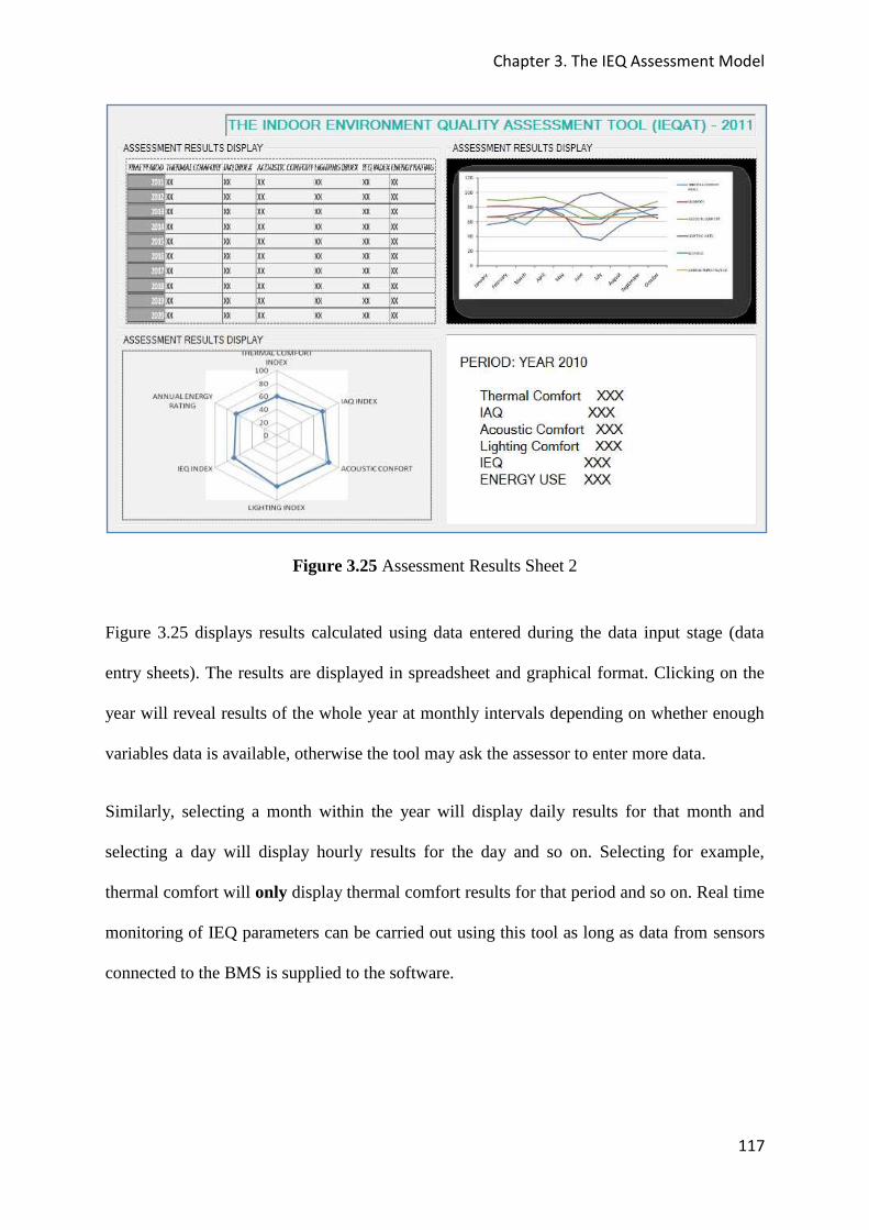
Chapter 3. The IEQ Assessment Model
117
Figure 3.25 Assessment Results Sheet 2
Figure 3.25 displays results calculated using data entered during the data input stage (data
entry sheets). The results are displayed in spreadsheet and graphical format. Clicking on the
year will reveal results of the whole year at monthly intervals depending on whether enough
variables data is available, otherwise the tool may ask the assessor to enter more data.
Similarly, selecting a month within the year will display daily results for that month and
selecting a day will display hourly results for the day and so on. Selecting for example,
thermal comfort will only display thermal comfort results for that period and so on. Real time
monitoring of IEQ parameters can be carried out using this tool as long as data from sensors
connected to the BMS is supplied to the software.
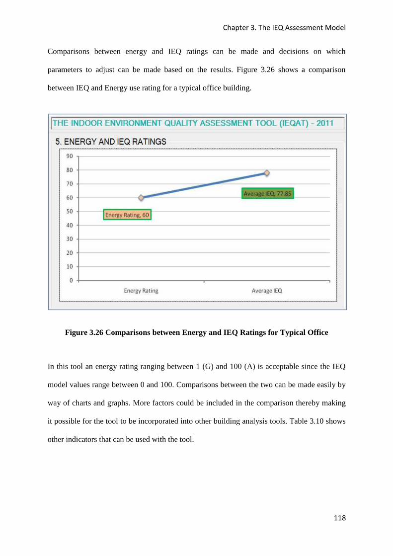
Chapter 3. The IEQ Assessment Model
118
Comparisons between energy and IEQ ratings can be made and decisions on which
parameters to adjust can be made based on the results. Figure 3.26 shows a comparison
between IEQ and Energy use rating for a typical office building.
Figure 3.26 Comparisons between Energy and IEQ Ratings for Typical Office
In this tool an energy rating ranging between 1 (G) and 100 (A) is acceptable since the IEQ
model values range between 0 and 100. Comparisons between the two can be made easily by
way of charts and graphs. More factors could be included in the comparison thereby making
it possible for the tool to be incorporated into other building analysis tools. Table 3.10 shows
other indicators that can be used with the tool.
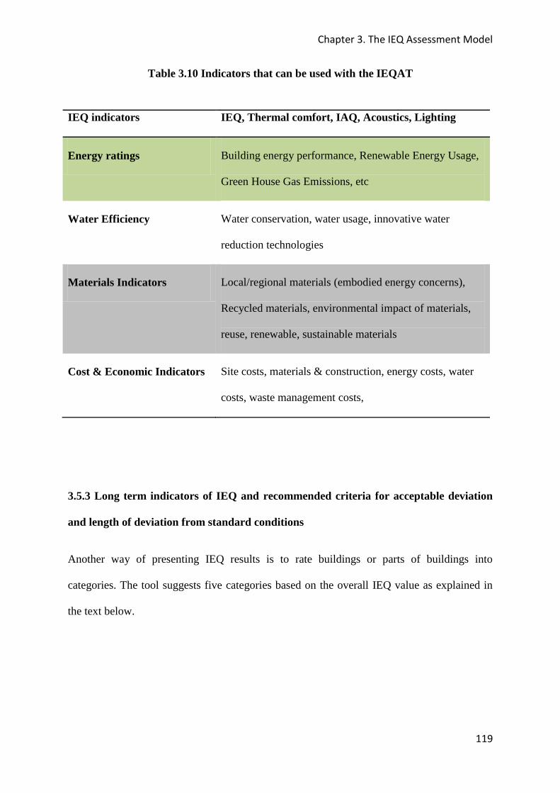
Chapter 3. The IEQ Assessment Model
119
Table 3.10 Indicators that can be used with the IEQAT
IEQ indicators IEQ, Thermal comfort, IAQ, Acoustics, Lighting
Energy ratings Building energy performance, Renewable Energy Usage,
Green House Gas Emissions, etc
Water Efficiency Water conservation, water usage, innovative water
reduction technologies
Materials Indicators Local/regional materials (embodied energy concerns),
Recycled materials, environmental impact of materials,
reuse, renewable, sustainable materials
Cost & Economic Indicators Site costs, materials & construction, energy costs, water
costs, waste management costs,
3.5.3 Long term indicators of IEQ and recommended criteria for acceptable deviation
and length of deviation from standard conditions
Another way of presenting IEQ results is to rate buildings or parts of buildings into
categories. The tool suggests five categories based on the overall IEQ value as explained in
the text below.
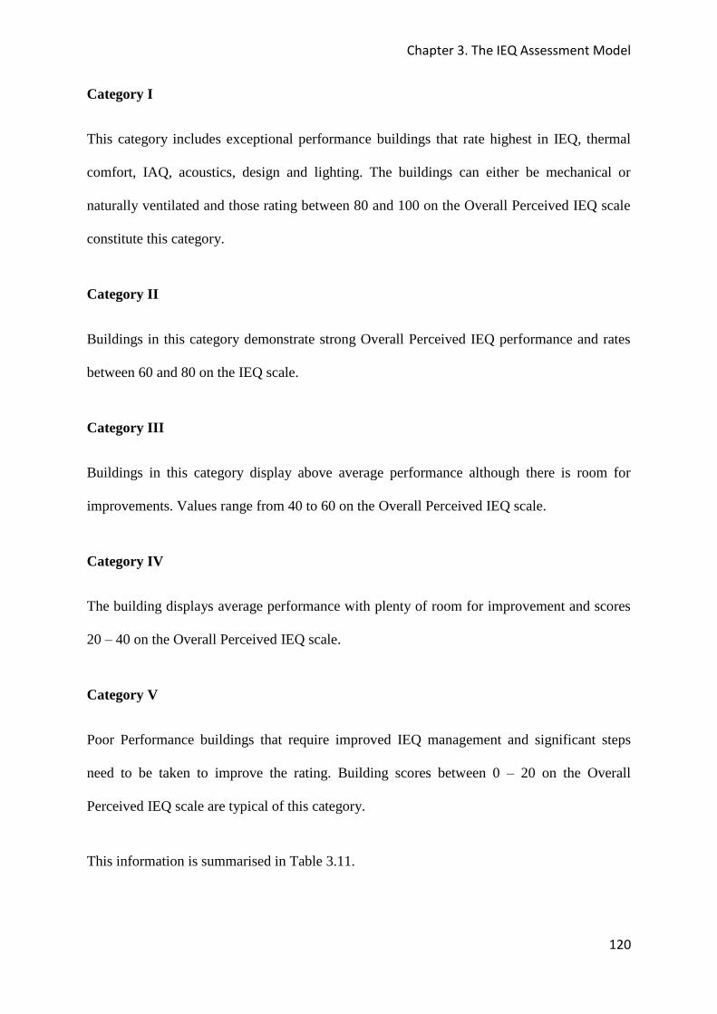
Chapter 3. The IEQ Assessment Model
120
Category I
This category includes exceptional performance buildings that rate highest in IEQ, thermal
comfort, IAQ, acoustics, design and lighting. The buildings can either be mechanical or
naturally ventilated and those rating between 80 and 100 on the Overall Perceived IEQ scale
constitute this category.
Category II
Buildings in this category demonstrate strong Overall Perceived IEQ performance and rates
between 60 and 80 on the IEQ scale.
Category III
Buildings in this category display above average performance although there is room for
improvements. Values range from 40 to 60 on the Overall Perceived IEQ scale.
Category IV
The building displays average performance with plenty of room for improvement and scores
20 – 40 on the Overall Perceived IEQ scale.
Category V
Poor Performance buildings that require improved IEQ management and significant steps
need to be taken to improve the rating. Building scores between 0 – 20 on the Overall
Perceived IEQ scale are typical of this category.
This information is summarised in Table 3.11.
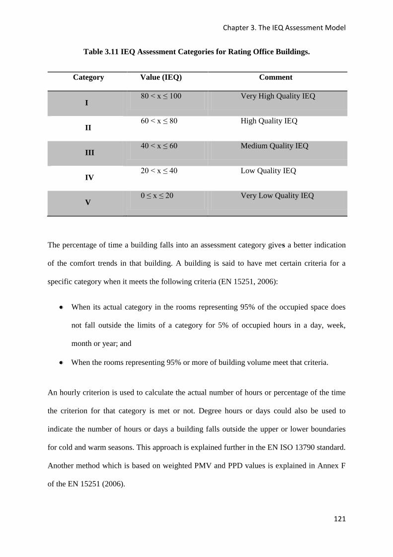
Chapter 3. The IEQ Assessment Model
121
Table 3.11 IEQ Assessment Categories for Rating Office Buildings.
Category Value (IEQ) Comment
I 80 < x ≤ 100 Very High Quality IEQ
II 60 < x ≤ 80 High Quality IEQ
III 40 < x ≤ 60 Medium Quality IEQ
IV 20 < x ≤ 40 Low Quality IEQ
V 0 ≤ x ≤ 20 Very Low Quality IEQ
The percentage of time a building falls into an assessment category gives a better indication
of the comfort trends in that building. A building is said to have met certain criteria for a
specific category when it meets the following criteria (EN 15251, 2006):
When its actual category in the rooms representing 95% of the occupied space does
not fall outside the limits of a category for 5% of occupied hours in a day, week,
month or year; and
When the rooms representing 95% or more of building volume meet that criteria.
An hourly criterion is used to calculate the actual number of hours or percentage of the time
the criterion for that category is met or not. Degree hours or days could also be used to
indicate the number of hours or days a building falls outside the upper or lower boundaries
for cold and warm seasons. This approach is explained further in the EN ISO 13790 standard.
Another method which is based on weighted PMV and PPD values is explained in Annex F
of the EN 15251 (2006).
Chapter 3. The IEQ Assessment Model
122
Figure 3.27 shows a typical assessment result sheet showing the percentage of time a building
falls into a particular category.
Figure 3.27 Assessment Results Sheet Showing % of time Office Space Falls into
Particular Category
Another way of displaying the results is shown in Figure 3.28 and this method can be used
for both real time and long term display of results. For real time monitoring the colour codes
are expected to change as the quality of the indoor environment changes from one category to
another.

Chapter 3. The IEQ Assessment Model
123
Figure 3.28 Real time or long term representation of office assessment results
Assessment of individual offices is straight forward. A different approach is required for
office complexes because more than one area is considered. An average rating for an office
complex is calculated as a weighted average of the assessment results for each type of office
based on the ratio of floor space occupied by each space.
The score for an office complex is given as:
荊継芸沈津鳥勅掴 噺 布鯨沈畦沈 惣┻ 惣層津沈退待
Alternatively:
荊継芸沈津鳥勅掴噺 釆磐荊継芸沈津鳥勅掴怠 抜 畦怠畦痛墜痛銚鎮卑 髪 磐荊継芸沈津鳥勅掴態 抜 畦態畦痛墜痛銚鎮卑髪 橋 ┸┼ ┸┼ ┸┼ ┸┼┼ ┸┼ ┻ ┸ ┼ ┻ ┸ ┼ 岫荊継芸沈津鳥勅掴仔 抜 畦仔畦痛墜痛銚鎮卑 惣┻ 惣匝
Figure 3.29 graphically illustrates the method used to assess more than one office / office
complex.

Chapter 3. The IEQ Assessment Model
124
Figure 3.29 Methodology for Assessment of Multiple Offices
3.6 CONCLUSIONS
The IEQAT has great potential to offer a long lasting solution to the problem of single index
IEQ based assessment of office buildings in the UK and worldwide. The main challenge is to
discover how much influence each of the four contributing factors has on the overall
perception of IEQ. Results from Chiang et al‘s Analytical Hierarchy Process (Chiang and
Lai, 2002) provide some insight into the relative importance of each of the contributory
factors. However the information needs to be verified and the tool developed in this chapter
needs to be optimised using selected case study office buildings. The methodology used to
verify the tool is described in Chapter 4 while Chapter 5 provides results of the case studies.
IEQ result Office X Section A Zone1 IEQ result Office X Section A Zone2 IEQ result Office X Section B Zone1
Floor area weighted average IEQ values
IEQ result for office Complex
Chapter 4. Research Methodology
125
4. Research Methodology
INTRODUCTION
The major purpose of this chapter is to outline the approach (methodology) used to discover
how much influence each of the predictors (proposed indoor environment variables) have on
perceived IEQ in office buildings. The exercise will help determine the relative importance of
each of the variables in determining perceived IEQ in the UK context and hence help
improve the IEQ tool proposed in Chapter 3. The chapter covers research study design,
selection of sample buildings, questionnaire design, measurement of physical variables
including equipment used and data analysis.
4.1 RESEARCH DESIGN
4.1.1 Selection of Research Design
Research design is defined by Trochim and Donnely (2006) as “a general plan” or “glue that
holds the research project together”. Several types of research designs have been proposed in
literature (Rogosa, 1978; Cook and Campbell, 1984; Trochim and Donnely, 2006) and they
are generally classified into three broad categories, namely the true experiments, quasi-
experiments and non experiments, depending on whether certain criterion is met or not. In
this thesis a flowchart illustrated in Figure 4.1 shows the decision process followed in order
to determine which type of experiment to use for the study. The solid lines indicate the path
followed in the selection of the appropriate type of experiment.
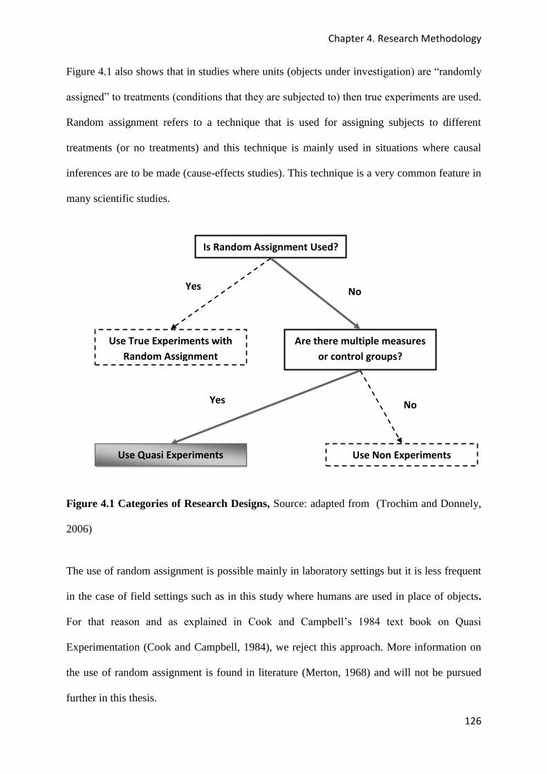
Chapter 4. Research Methodology
126
Figure 4.1 also shows that in studies where units (objects under investigation) are “randomly
assigned” to treatments (conditions that they are subjected to) then true experiments are used.
Random assignment refers to a technique that is used for assigning subjects to different
treatments (or no treatments) and this technique is mainly used in situations where causal
inferences are to be made (cause-effects studies). This technique is a very common feature in
many scientific studies.
Figure 4.1 Categories of Research Designs, Source: adapted from (Trochim and Donnely,
2006)
The use of random assignment is possible mainly in laboratory settings but it is less frequent
in the case of field settings such as in this study where humans are used in place of objects.
For that reason and as explained in Cook and Campbell’s 1984 text book on Quasi
Experimentation (Cook and Campbell, 1984), we reject this approach. More information on
the use of random assignment is found in literature (Merton, 1968) and will not be pursued
further in this thesis.
Is Random Assignment Used?
Use True Experiments with
Random Assignment
Are there multiple measures
or control groups?
Use Quasi Experiments Use Non Experiments
Yes
Yes
No
No
Chapter 4. Research Methodology
127
Other types of study designs had to be considered and these included non experiments and
quasi experiments (Figure 4.1). Non experiments are designs used in studies where no
multiple measures or control groups are used, and again in our study office occupants were
subjected to several IEQ parameters and this approach was rejected. Campbell and Cook
(1984) placed special emphasis on a third type of experiments that have treatments, outcomes
and experimental units, but do not use random assignment to create comparisons from which
treatment caused change is inferred. These types of experiments have been referred to as
quasi experiments and they can be used in prediction, correlation and causal studies.
Quasi experiments are traditionally divided into three groups, i.e. the non equivalent group
designs, interrupted time series and correlational designs. Non-equivalent group designs are
designs in which responses of a treatment group are measured before and after treatment for
example, the effects of changing the temperature of a room by one degree Celsius on thermal
comfort is measured before and after a central heating system is turned on. Interrupted time
series methods are designs in which the conditions are measured at many time intervals
before a treatment and then the measures taken at many time intervals again after the
treatment has been administered. For example IEQ acceptability or thermal comfort is
measured daily for a month then measured again daily for a month after a working cooling
system in put in place. Correlational methods most often refer to efforts at investigating co
occurrence (or causal inference in some cases) based on measures taken all at one time with
differential levels of both effects and exposures to presumed causes being measured as they
occur naturally without any experimental intervention.
The investigation of the effects of indoor environment conditions on an individual’s
perception of the indoor environment in an office building is an example of a research study
that is carried out in a natural setting. Correlational designs are relatively easy to conduct
Chapter 4. Research Methodology
128
although they leave the actual reasons for association between dependent and independent
variables quite unclear. More credibility is attributed to tests based on actual field studies as
they are deemed to be more representative of the natural situation (Cook and Campbell,
1984).
Passive Observational Methods (POM) are forms of correlational methods that deal with
“investigating covariance or inferring cause based on observations of concomitances and
sequences as they occur naturally without the obvious advantages of deliberate manipulation
and controls associated with experiments” (Cook and Campbell, 1984). In these methods
manipulable controls are substituted with naturally occurring ones, nevertheless the aim is to
discover whether variables covary or not, and whether there is any correlation or not.
POMs can also be used on non equivalent groups i.e. groups that differ from each other in
many ways other than the presence of the treatment or phenomena whose effects we are
trying to investigate. For example, in this study human subjects in the indoor environment
have many different characteristics that make them respond differently to indoor environment
conditions. Such characteristics would otherwise be absent when dealing with say, human
manikins, etc. Quasi experimentation is by no means a way of justifying the use of inferior
research designs, it is a powerful tool that can be used effectively in field studies in social
sciences and engineering alike (Lowe, 2009). Before the process of developing the structure
of the study design begins a clear distinction between the use of passive observational
approaches to describe events, infer causal relations and to forecast or predict outcomes had
to be made. This distinction is also explained in Campbell & Cook (1984). Moreover one can
find explicit distinctions between predictive regression (forecasting) and structural regression
(cause-effect) as explained in Trochim and Donnely (2006) and Panacek and Thomoson
(1995) respectively. Descriptive statistics are fairly straight forward and they will not be
explored further in this section.

Chapter 4. Research Methodology
129
It is alleged by Panacek and Thomoson (1995) that recent applied statistical analyses in social
research have ignored any distinction between forecasting and causal inference with
devastating effect . For purely forecasting purposes, it will not matter what the true causal
path is as long as the predictor acts as a symptom (Vasconcelos et al, 1998; Merton,
1968; Lowe, 2009). In this case the area of interest is in how “powerful” each predictor is in
predicting the acceptability of the indoor environment regardless of whether the presumed
causal variable is a complex composite of which only a part produces the correlation.
However in causal inference it is important for a “treatment” given to an individual or group
to “work”, i.e. to be abrupt, precisely dated and probably cause change, as if it was a planned
intervention (true experiment) (Nelder and McCullagh, 1989). A methodical development of
correlational studies is presented in Section 4.1.2.
4.1.2 The Methodological Basis of Correlational Designs
The methodology begins with a case in Figure 4.2 (a) where no distinction is made between
dependent and independent variables, and no prior knowledge is supposed for the
interrelations among predictor variables (X1-5), and the dependent variable (O). Correlational
research designs are founded on the assumption that reality is best described as a network of
interacting and mutually causal relationships where a web of relationships in which
everything affects or is affected by everything else exists. Thus, as a rule the dynamics of a
system (how individual parts of the whole system affect other parts) is more important than
causal relationships as seen in Vasconcelos et al (1998)’s Path Analysis Approach for the
Multivariate Analysis of Infant Mortality Data.
Chapter 4. Research Methodology
130
In Figure 4.2 (b), variable O can be determined as dependent or influenced by the others i.e.
X1-5. When no distinction is made between dependent and independent variables, factor
analysis (exploratory and or confirmatory shown in Figure 4.2 (c)) is the adequate model to
use. This statistical procedure identifies underlying patterns of variables and their
interrelations. When a large number of variables are correlated and high inter-correlations are
present then a common underlying factor may be present.
Once confirmation of independent and dependant variables is carried out or prior knowledge
of the relationship is known (This is the point where this research begins) the need to
determine whether the aim of the research is to infer cause, determine covariance or
investigate correlations becomes important. Two designs used to make cause-effect
statements using correlational methods are path analysis and cross-lagged panel designs.
These methods are not described in this research but they can be found in Cook & Campbell
(1984) and they are also written about extensively in literature (Nelder and McCullagh,
1989; Karunaratne and Elston, 1998; Wong et al, 2007; Hahn and Soyer, 2005; Movellan,
2003; Fairfax County Department of Systems Management for Human Services, 2003). For
regression and predictive modelling (correlational) the most appropriate method is the
Multivariate Regression analysis. The path followed in the selection of the multivariate
regression model is highlighted in Figure 4.2.
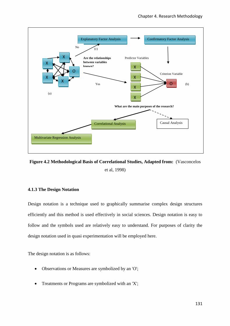
Chapter 4. Research Methodology
131
Figure 4.2 Methodological Basis of Correlational Studies, Adapted from: (Vasconcelos
et al, 1998)
4.1.3 The Design Notation
Design notation is a technique used to graphically summarise complex design structures
efficiently and this method is used effectively in social sciences. Design notation is easy to
follow and the symbols used are relatively easy to understand. For purposes of clarity the
design notation used in quasi experimentation will be employed here.
The design notation is as follows:
Observations or Measures are symbolized by an 'O';
Treatments or Programs are symbolized with an 'X';
X
X
X
X
O
Explanatory Factor Analysis Confirmatory Factor Analysis
X
O
X
X
X
What are the main purposes of the research?
Correlational Analysis
Are the relationships between variables known?
Multivariate Regression Analysis
Causal Analysis
Predictor Variables
Criterion Variable
(a)
(b)
(c)
Yes
No
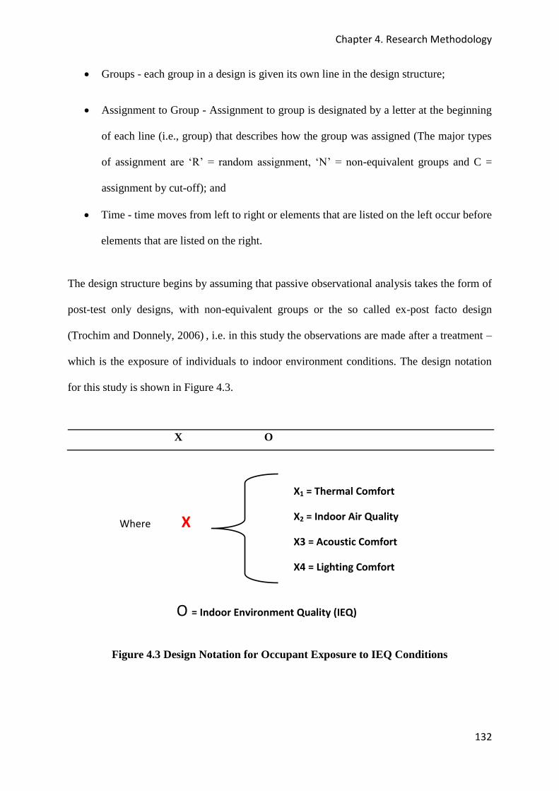
Chapter 4. Research Methodology
132
Groups - each group in a design is given its own line in the design structure;
Assignment to Group - Assignment to group is designated by a letter at the beginning
of each line (i.e., group) that describes how the group was assigned (The major types
of assignment are ‘R’ = random assignment, ‘N’ = non-equivalent groups and C =
assignment by cut-off); and
Time - time moves from left to right or elements that are listed on the left occur before
elements that are listed on the right.
The design structure begins by assuming that passive observational analysis takes the form of
post-test only designs, with non-equivalent groups or the so called ex-post facto design
(Trochim and Donnely, 2006) , i.e. in this study the observations are made after a treatment –
which is the exposure of individuals to indoor environment conditions. The design notation
for this study is shown in Figure 4.3.
X O
Figure 4.3 Design Notation for Occupant Exposure to IEQ Conditions
X1 = Thermal Comfort
X2 = Indoor Air Quality
X3 = Acoustic Comfort
X4 = Lighting Comfort
Where X
O = Indoor Environment Quality (IEQ)
Chapter 4. Research Methodology
133
This is the simplest form of design which would otherwise be uninformative as far as causal
inference is concerned but highly useful for predictive correlational studies. As one can see
the groups are subjected to a treatment (indoor thermal conditions, air quality issues,
acoustics, lighting and workspace design conditions) and observations (IEQ acceptance) are
made thereafter. At first glance the notation appears to reflect a non experiment, however
since we study more than one office and each office is subjected to different IEQ conditions,
then the study ceases to become a post test only quasi experiment. In the next section the
selection of sample buildings is discussed.
4.2 SELECTION OF SAMPLE BUILDINGS
In this study representative samples were drawn from a wide list of Hoare Lea and other
offices across the UK. Sampling was necessary because it provided a cheaper, faster and
practical way of studying office buildings (Campbell and Stanely, 1963).
The samples were selected using the probability sampling (stratified) approach because of the
following advantages over non random sampling:
It allows us to calculate the precision of the estimates obtained from the sample
and to specify the sampling error; and
It allows us to generalise the sample results to the target population
Probability sampling is also more accurate than a census of the entire population because the
smaller sampling operation lends itself to the application of more rigorous controls, thus
ensuring better accuracy (Fairfax County Department of Systems Management for Human
Services, 2003). These rigorous controls allowed the reduction of non sampling errors such as
non response problems, questionnaire design flaws, and data processing and analysis errors.

Chapter 4. Research Methodology
134
Sampling was especially important for questionnaire administration because a relatively long
and difficult questionnaire could be administered to a sample more easily than a relatively
short and simple questionnaire can be administered to the entire population (Campbell and
Stanely, 1963). The samples that were selected consisted of offices that were different from
each other in many important ways and this is crucial if sound generalizations to the target
population are to be made (Oppenheim, 1992; Wong et al, 2007). Before doing this there was
need to start by defining what characteristics or levels were typical of office environments
(target population) in the UK. In general offices are defined by at least one of the following
characteristics:
Office design - type of office e.g. open plan, cellular, its orientation, the type (open
plan or cellular), floor level, the level of furnishings, age of property, building fabric,
the spatial arrangements of walls, partitions, and equipment in relation to fixed
elements like windows and heating, ventilation and air conditioning. This leads to the
grading of offices into grade A, B and C. Grade A offices are spacious and furnished
with high-quality finishes, flexible layout, large floor plans, well decorated lobbies
and circulation areas, effective central air conditioning, good lift services zoned for
passengers and goods deliveries, professional management, and parking facilities are
normally available; Grade B offices are of ordinary design with good quality finishes,
flexible layout, average-sized floor plates, adequate lobbies, central or free-standing
air-conditioning, adequate lift services, good management, and parking facilities are
not essential; and Grade C offices are those plain with basic finishes, less flexible
layout, small floor plates, basic lobbies, hardly any central air-conditioning, barely
adequate or inadequate lift services, minimal to average management and no parking
facilities (Wong et al, 2007);

Chapter 4. Research Methodology
135
HVAC system in place – whether offices are naturally ventilated, mechanical, mixed
mode or have personalised ventilation systems (PVS);
Design parameters – Temperature, lighting, acoustics, IAQ, vibration, day lighting
ranges (values) allowable for purposes of design or based on IEQ criteria used; and
Location – whether they are located in urban (towns, cities, conurbations), peri urban
(locations surrounding urban centres, between rural and urban areas) or rural areas
(villages, hamlets, countryside), the actual city or region where they are sited, whether
they are in a university campus, military base, airport terminal, etc.
Typical offices were then categorized into the following mutually exclusive groups from
which three were selected:
Mechanical or naturally ventilated offices;
Grades A, B or C offices;
Urban or Rural Location;
Design standards employed e.g. part L Building Regulations 2006, etc, related to date
built; and
Cellular or open plan type.
The Granby House office in Nottingham, the Marsh-Growchoski & Associates office suite
and the Leeds Town Centre House were selected. The resulting variation is illustrated in
Table 4.1 and the specific characteristics of selected case study buildings are discussed in
Chapter 5. The results of the three buildings are not expected to provide enough information
from which generalisations across other office buildings in the UK can be made. They will
however provide a good foundation on which future studies can be made and these could
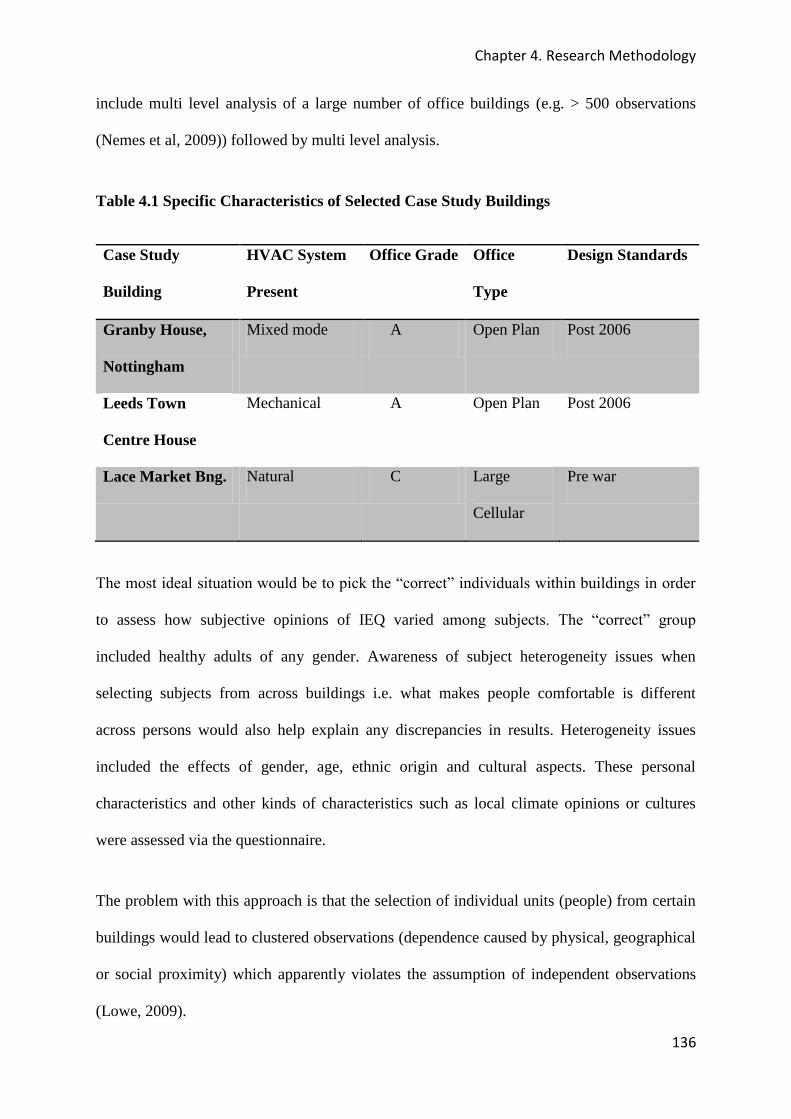
Chapter 4. Research Methodology
136
include multi level analysis of a large number of office buildings (e.g. > 500 observations
(Nemes et al, 2009)) followed by multi level analysis.
Table 4.1 Specific Characteristics of Selected Case Study Buildings
Case Study
Building
HVAC System
Present
Office Grade Office
Type
Design Standards
Granby House,
Nottingham
Mixed mode A Open Plan Post 2006
Leeds Town
Centre House
Mechanical A Open Plan Post 2006
Lace Market Bng. Natural C Large
Cellular
Pre war
The most ideal situation would be to pick the “correct” individuals within buildings in order
to assess how subjective opinions of IEQ varied among subjects. The “correct” group
included healthy adults of any gender. Awareness of subject heterogeneity issues when
selecting subjects from across buildings i.e. what makes people comfortable is different
across persons would also help explain any discrepancies in results. Heterogeneity issues
included the effects of gender, age, ethnic origin and cultural aspects. These personal
characteristics and other kinds of characteristics such as local climate opinions or cultures
were assessed via the questionnaire.
The problem with this approach is that the selection of individual units (people) from certain
buildings would lead to clustered observations (dependence caused by physical, geographical
or social proximity) which apparently violates the assumption of independent observations
(Lowe, 2009).
Chapter 4. Research Methodology
137
Violation of this assumption would lead to the following consequences:
Violation implies that the information from each IEQ observation ‘overlaps’ or
‘duplicates’ to some extent the information from other ones, making the total amount of
information smaller than if the observations had been independently selected. In other
words the ‘effective’ number of observations is smaller than the number of individual
respondents;
If non-independence is ignored estimated standard errors become too small, and
hypothesis testing becomes too lenient (the so called alpha-inflation); and therefore the
estimated IEQ coefficients or weightings may be biased;
Ignoring the factors causing non-independence results in poorly specified models and
again in biased coefficients (omitted variable bias); and
Since clustering implies the distinction of different levels at which the empirical world
can be described one needs to redefine the relationship between characteristics of units at
a different level, a higher level, i.e. we need to use multi level analysis methods.
Such distinctions have been explicitly used since 1897 (Campbell and Stanely, 1963). Multi
level modelling has its limitations. It is only a potential solution for violation of the
assumption of independent observations, not for all other kinds of problems (violations of
other assumptions, sampling defects, measurement defects, etc.) We therefore need to assess
whether we need multi level modelling or not as it could yield very little difference in some
cases. Multi level analysis will be discussed further in Chapter 6.

Chapter 4. Research Methodology
138
4.3 DATA COLLECTION EXERCISE - THE QUESTIONNAIRE
4.3.1 Motivation for the Questionnaire
The overall aim of the questionnaire was to identify patterns in the relationship between IEQ
rating and the proposed predictor variables. The questionnaire was needed to identify and
collect occupant’s subjective opinion of the microclimatic conditions of the space in which
they worked. It also needed to capture the occupant’s opinion (rating) of the indoor
environment and their opinion of several parameters that are thought to influence perceived
IEQ at their workstations.
Only those occupants (group) who were present in the offices on the days of the survey were
asked to complete the questionnaire to facilitate monitoring. All respondents were pre warned
five months in advance and then reminded a week before the actual survey was carried out.
The questionnaires were completed while occupants worked in their respective work stations.
The questions took approximately 10 – 12 minutes to complete and the responses were
collected and analysed later. Monitoring of IEQ parameters affecting comfort was carried out
throughout the working day using standard equipment as explained in Section 4.4.2. In this
way the data collected from the occupants could be compared to field measurements hence
the questionnaire results could be validated.
Contradictions between survey and measured data could arise due to poor positioning of field
sensors, low accuracy of apparatus collecting physical data and poor questionnaire structure.
In some cases the health and well being of respondents (sensitivity to internal environment
parameters or lack of due to disease, etc) could also affect subjective responses. Such factors
would be considered where inconsistencies in the data existed. Once the questionnaire results
were validated using field measurements, regression analysis could be used to determine the
Chapter 4. Research Methodology
139
relative weightings of each of the four main parameters affecting IEQ hence the proposed
IEQ model could be improved or verified. The model however cannot be used to replace
current building regulations or standards, but it can be used as a guide on how much
sacrifices in human comfort could be associated with proposed energy efficiency measures.
A group administered questionnaire method was used to collect data because it:
is fast;
is a low cost technique that required little in terms of equipment and personnel;
offers high response rates since questions are handed out and collected after the
exercise (personal contact);
is fairly easy to judge the quality of the responses; and
It is also possible for respondents or the administrator to make clarifications where
necessary (Hahn and Soyer, 2005).
The disadvantages of the questionnaire methods include lack of quick turnarounds which
limits the number of questionnaires that can be administered by one individual (the
administrator). Long questionnaires are also not always possible as they can be costly, time
consuming, demand more effort from the respondents and may lead to poor responses or
unreliable responses (Campbell and Stanely, 1963; Cook and Campbell, 1984). Although no
issues with privacy are expected the questionnaire responses needed to be made as
anonymous as possible, and this was explained to the participants. Open ended questions
were generally avoided, except in optional circumstances where clarifications of responses
were required, as responses could be confusing to the statistician (Trochim and Donnely,
2006). Lack of open ended questions however could mean the freedom and spontaneity of
answers is lost. The opportunity to probe even further could also be lost.

Chapter 4. Research Methodology
140
Post Occupancy Evaluation Methods (POEM) in buildings employ a range of techniques such
as questionnaires, interviews, focus groups, measurement and observation. Questionnaires are
commonly used in buildings studies to get feedback about the indoor environment from the
occupants. In the UK the Building Use Studies (BUS) questionnaire is the most common tool
used to evaluate IEQ, health, wellbeing and productivity of occupants against well
established benchmarks. BUS questionnaires have been used to assess comfort in green
buildings and the results of such studies have helped eliminate past mistakes that have caused
poor indoor environment conditions in those buildings (Leaman and Bordass, 2007). A
comprehensive study carried out in office in the city of Melbourne used the BUS study
questionnaire and it highlighted that the productivity of office building occupants can
potentially be enhanced through good building design, and provision of a high quality,
healthy, comfortable and functional interior environment, that takes account of basic
occupant needs (Paevere and Brown, 2008). This adds to the fact that questionnaires play an
important part of building assessments because they provide feedback on the actual
performance of buildings.
The Stockholm Indoor Environment Questionnaire is a standard social questionnaire that was
developed to assess indicators of indoor environment such as air quality, thermal climate,
noise and illumination (Engvall et al, 2003). The questionnaire was tested and validated with
much success in 350 apartments in Sweden confirming that it can be used as a tool of choice
for decision makers when making priorities and identifying ”risk” buildings.
Questionnaires have also been used in many other studies comparing subjectively assessed
IEQ to model assessed IEQ as explained in Chapter 3 (Wong et al, 2007, Lai et al, 2009,
Leaman and Bordass, 2007; Paevere and Brown, 2008). The EN15151 standard contains
sample question structures that should be used when assessing IEQ in buildings and in this
Chapter 4. Research Methodology
141
thesis the “types” of questions used are based on recommendations of the standard
(EN15251, 2006).
4.3.2 Questionnaire Structure
The Questionnaire is divided into two sections. Section 1 tries to assess the influence of
perceived thermal comfort, indoor air quality, acoustic, visual & workplace design on the
overall IEQ during a particular season of the year. [Heating season (November - April) and
Cooling season (May - October)]. Section 2 contains personal factors such as occupant level
of satisfaction with the tasks or their general motivational levels. These questions will be
optional but they may help to explain any discrepancies that may exist between field
measurements and subjective opinions of respondents.
SECTION 1
This section is about building comfort.
Question 1 asks about the details of a particular building. The name of the building, the floor
and the season will help explain the conditions the occupants found themselves in. Clear floor
plans are provided for respondents to determine the exact location of their workstations. This
will help explain environmental conditions prevailing within each area and help correlate to
field and simulation results. This will also help validate the answers given by the respondents
and hopefully indicate any variations in perceived comfort levels with floor level, building
location, season, microclimatic conditions, etc.
Question 2 asks respondents to provide an indication of whether or not they accept the
environment they work in. This question provides an insight into the quality of the building’s
indoor space (all proposed five factors plus other contributing factors) and is a result of
Chapter 4. Research Methodology
142
factors such as the performance of the buildings’ HVAC system, the performance of the
building fabric, the orientation and location of the building, floor levels, the “state of mind”
of the occupants, etc.
A dichotomous assessment scale will be used to determine the respondents’ acceptability of
the quality of the indoor environment (IEQ). The questions will be phrased such that they will
be easier to understand and respond to by the occupants, for example “Is the IEQ of your
work environment acceptable to you?” with dummy variables 0, 1 (0 = No; 1 = Yes) as
answer options is self explanatory. Providing a dichotomous scale will help make a clear cut
distinction between acceptability and non acceptability of the conditions. This will help avoid
overlapping answers or confusion when analysing data. The validity of their responses
(dummy variables) will be assessed using a parallel Visual Analogue Scale (VAS) (Houser
and Tiller, 2003). A validity check question “How would you rate the quality of the indoor
environment in your work area?” (Indicate your answer using values 1 = Poor to 5 = Good;
on the Visual Analogue Scale; would help verify responses.
Question 3 asks for direct feedback on their perception of the thermal environment. An
ASHRAE assessment scale (Benton et al, 1990) which is based on the semantic differential
scale, and which takes into account clothing levels, activity levels, dry bulb temperature,
mean radiant temperature, relative humidity and air flow rates is provided for mechanically
ventilated office. Semantic differential scales are based on the understanding that people use
evaluation, potency, and activity to evaluate words and phrases (Trochim and Donnely,
2006). In this questionnaire “evaluation” is used to describe thermal comfort. A VAS which
is used to evaluate naturally ventilated offices buildings is provided at the end of the
questionnaire.
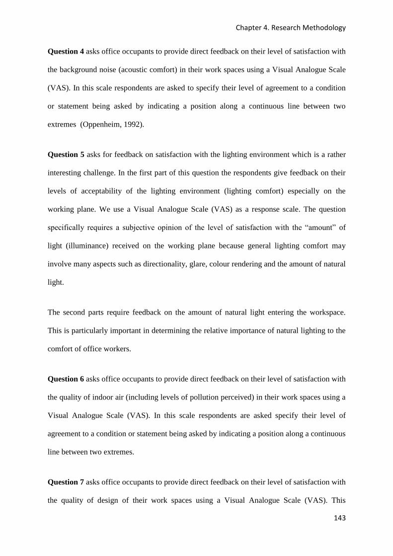
Chapter 4. Research Methodology
143
Question 4 asks office occupants to provide direct feedback on their level of satisfaction with
the background noise (acoustic comfort) in their work spaces using a Visual Analogue Scale
(VAS). In this scale respondents are asked to specify their level of agreement to a condition
or statement being asked by indicating a position along a continuous line between two
extremes (Oppenheim, 1992).
Question 5 asks for feedback on satisfaction with the lighting environment which is a rather
interesting challenge. In the first part of this question the respondents give feedback on their
levels of acceptability of the lighting environment (lighting comfort) especially on the
working plane. We use a Visual Analogue Scale (VAS) as a response scale. The question
specifically requires a subjective opinion of the level of satisfaction with the “amount” of
light (illuminance) received on the working plane because general lighting comfort may
involve many aspects such as directionality, glare, colour rendering and the amount of natural
light.
The second parts require feedback on the amount of natural light entering the workspace.
This is particularly important in determining the relative importance of natural lighting to the
comfort of office workers.
Question 6 asks office occupants to provide direct feedback on their level of satisfaction with
the quality of indoor air (including levels of pollution perceived) in their work spaces using a
Visual Analogue Scale (VAS). In this scale respondents are asked specify their level of
agreement to a condition or statement being asked by indicating a position along a continuous
line between two extremes.
Question 7 asks office occupants to provide direct feedback on their level of satisfaction with
the quality of design of their work spaces using a Visual Analogue Scale (VAS). This

Chapter 4. Research Methodology
144
includes spatial arrangements, size of workspace, aesthetics, quality of furnishings, etc. Like
in questions 4 - 6 respondents are asked specify their level of agreement to a condition or
statement being asked by indicating a position along a continuous line between two extremes.
Question 8 asks about discomfort caused by the presence of any local discomfort factors.
This question will help eliminate any influences due to the presence of local discomfort
factors.
SECTION 2
The effects of personal characteristics such as gender, age, ethnic origins, cultural aspects and
beliefs (idiosyncratic issues) are required to help validate the subjective, quantitative data
given in section 1. There is an influence of subject heterogeneity that needs to be generalised
across samples, i.e. what makes people comfortable is different across persons.
For example specifying the gender of the occupant may help to explain potential differences
in opinion of the buildings thermal performance due to differing dress codes or simply
gender. Age and health may also play a role in a person’s perception of the indoor
environment but these effects will be addressed further in the multilevel analysis of data in
future studies. Please refer to Appendix 2 for the actual questionnaire.
To investigate how occupants perceived their indoor environment at “that time” a
questionnaire was administered during the working days after every worker had had time to
settle down and adapt in some way to their environment. In order to verify the responses spot
checks of IEQ parameters was carried out on the working plane, about 0.8m above the floor
level as shown in Figure 4.4.
The working plane was a representative measuring point for every individual.
Chapter 4. Research Methodology
145
Figure 4.4 Diagram showing typical layout of the working plane
4.4 DATA COLLECTION EXERCISE – PHYSICAL MEASUREMENTS
Monitoring of the indoor environment parameters was carried out during questionnaire
administration in order to check the validity of the responses given by occupants. The
measured data was used to calculate microclimatic conditions prevailing in each work space
using the proposed IEQ model. The indoor microclimate varies in both space and time across
rooms and buildings due to, for example uneven distribution of heat or ventilation air by the
HVAC systems (Stanton et al, 2004). A converging-operations approach where subjective
assessments from the questionnaire are compared against measured quantities was introduced
in order to determine whether questionnaires provided a true reflection of the prevailing
comfort conditions in the building. Spatial considerations were taken into account and
instruments were strategically placed to represent the actual location of the worker or a group

Chapter 4. Research Methodology
146
of workers in a space (Benton et al, 1990). Therefore we can say the space was divided into
units similar to a grid with each workstation representing a unit area (within the grid). Studies
by Wong et al and others have also identified the working plane as the best to locate sensors
(Wong et al, 2007).
Temporal considerations were also of paramount importance if we were to understand the
patterns that existed in those spaces throughout the day, for example data on daily
temperature profiles in the Leeds office had to be collected for at least a full day prior to the
monitoring exercise to get a “feel” of the temperature distribution within the office. The
reliability of the data collected depends on the instruments used to collect the data and the
measurement strategy adopted as explained in the previous chapter. For example early
thermal comfort variables measurement instruments had wider ranges of error than those
available today, particularly those for measuring air velocity (CIBSE, 1986). However, it is
generally accepted that modern thermal sensors are adequately accurate, especially if they are
selected and used in accordance with guidelines (ISO-7726, 1988) provided by professional
organisations and standards (ASHRAE, 2005; EN 15251, 2006). A detailed description of
instrumentation used to evaluate indoor environment conditions is presented in Section 4.4.2.
4.4.1 Parameters to Measure
Thermal Comfort Parameters
The relative accuracy of the PMV model depends on the reliability of the four physical
inputs, the instruments used to collect the data and the measurement strategy adopted. The
most recent methods employ better techniques such as taking repeated measurements in large
and representative sample of locations (Charles, 2003) therefore the validity of the PMV
model is not seriously compromised by measurement error.

Chapter 4. Research Methodology
147
Six parameters affecting thermal comfort in intermediate thermal environments have been
identified in Chapter 2 as air temperature, mean radiant temperature, humidity, air velocity,
clothing levels and activity levels (metabolic heat production) (Fanger, 1973). The
parameters are measured in order to compute PMV and PPD values which can then be
compared with questionnaire data. Table 4.2 is a summary of thermal comfort parameters that
were measured, the data collection points and data collection procedures used.
Table 4.2 Thermal Comfort Parameters Investigated
Measure Sampling Season Sampling
location
Data Collection Method
Air Temperature Heating/Cooling Working
Plane (Head
level)
Continuously data Logged
Mean Radiant
Temperature
Heating/Cooling Working
Plane
Assumed to be equal to Air
temperature*
Relative
Humidity
Heating/Cooling Working
Plane
Handheld instruments that allow
multipoint logging
Air Velocity Heating/Cooling Working
Plane
Continuously data Logged
Clothing Levels Heating/Cooling Working
Plane
Direct observation
Activity Levels Heating/Cooling Working
Plane
Direct observation
*Assumption that no significant variation in air temperature and mean radiant temperature – potential source of error.
Chapter 4. Research Methodology
148
Clothing insulation is measured in units of ‘clo’ (Gagge, 1940). Establishing the insulating
properties of clothing is a time-consuming and detailed process that is usually conducted in
laboratory experiments devoted to this purpose. As it is not practical to directly measure
clothing insulation in most thermal comfort studies, researchers generally estimate these
values using tables that have been developed from clothing insulation studies (ASHRAE,
1992).
Some researchers assume an average clo value for all occupants, based on the season and
climate of the study location, and typical clothing ensembles for office work (typically 0.35-
0.6 clo in summer, and 0.8-1.2 clo in winter). Clothing insulation levels in this study were
obtained by completing the occupants complete garment checklist, which was then used to
select a more appropriate clo value for the group, (or separate clo values for each participant).
Activity level is measured in terms of metabolic rate, or ‘met’ (Gagge, 1940). The most
accurate method for determining met is through laboratory studies, where heat or oxygen
production is measured for participants conducting specific activities (Havenith,
2008; Olesen and Parsons, 2002; Parsons, 2008). Alternatively, the participant’s heart rate
can be measured and compared to previously developed tables of heart rate for specific
activities. All of these methods, however, are time-consuming and invasive, and are generally
not practical for use by thermal comfort researchers. Instead, these researchers rely on
estimates, based on tables of met rates for specific activities and occupations, developed from
laboratory studies (EN-ISO7730, 2005). In most studies, an average met rate is assumed for
the group (usually 1.2 met for sedentary office work). Met values were estimated in this study
by observing occupants as they carried out their normal duties (activities) and the information
obtained was used to develop a more accurate average for the group, (or individualised met
estimates for each participant).

Chapter 4. Research Methodology
149
Other Parameters – IAQ, Lighting and Acoustics
Carbon dioxide concentrations were collected at strategic locations at working plane level
(see Figure 4.1) to determine IAQ and pollution due to bio effluents. Illuminance levels (lux)
were also measured on a working plane in order to estimate the levels of both artificial and
natural lighting received in the offices. A-weighted sound levels were used to estimate the
levels of background noise within the spaces. An analysis of the source and nature of the
background noise will also be analysed using critical listening. Table 4.3 is a summary of
IAQ, lighting and acoustics parameters that were monitored.
Table 4.3 Summary of IAQ, Lighting and Acoustics monitored
Measure Sampling Season Sampling location Data Collection
Method
Carbon dioxide
concentrations
Heating/Cooling Working Plane Continuously data
Logged
Iluminance Heating/Cooling Working Plane Handheld devices,
Continuously data
Logged
Background
Noise Levels
Heating/Cooling Working Plane Handheld devices
4.4.2 Monitoring Exercise and Equipment Used
Hardware used in this exercise consisted of a data logger connected to several analogue
sensors. The sensors were wired to the data logger limiting the distance between the two and
forcing the data collection exercise to take longer and forcing the use of handheld devices to
carry out spot measurements in other parts of the space. The University of Nottingham only
orders instruments from suppliers with a good track history in supplying top of the range
instruments. The equipment and software used are explained in the following paragraphs.

Chapter 4. Research Methodology
150
The Data logger DT500 Series – Logging Data
Figure 4.5 Datataker DT 500 3 series data logger
A Datataker DT500 data logger (3 series) with adequate memory capacity (1,390,000 data
points) and up to 37 channels was used to log room air temperature, illuminance, CO2
concentrations and air velocity during the monitoring exercise. The data taker was calibrated
in February 2010. The DT500 is DC powered with voltages ranging from 11 to 24Vdc. It
also has an internal 6V battery that can last up to 10 hours between charges making it
possible to move the data logger between sites without interrupting data logging activities.
An additional internal back up battery (3V, 1/2AA lithium) is available for internal data
storage back up. The data logger supports a wide range of sensors including thermocouples,
RTDs, Thermisters and Bridge sensors. The accuracy details of the DT500 are as follows:
Measurement of DC Voltage is at approx 0.15% at 25°C and 0.25% between -45 and
60°C;
Measurement of DC Current is at approx 0.25% at 25°C and 0.35% between -45 and
60°C; and
Measurement of DC Resistance is at approx 0.20% at 25°C and 0.30% between -45
and 60°C.
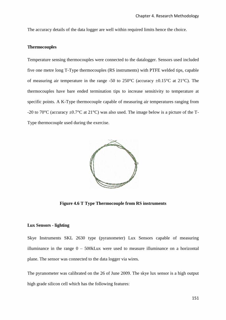
Chapter 4. Research Methodology
151
The accuracy details of the data logger are well within required limits hence the choice.
Thermocouples
Temperature sensing thermocouples were connected to the datalogger. Sensors used included
five one metre long T-Type thermocouples (RS instruments) with PTFE welded tips, capable
of measuring air temperature in the range -50 to 250°C (accuracy ±0.15°C at 21°C). The
thermocouples have bare ended termination tips to increase sensitivity to temperature at
specific points. A K-Type thermocouple capable of measuring air temperatures ranging from
-20 to 70°C (accuracy ±0.7°C at 21°C) was also used. The image below is a picture of the T-
Type thermocouple used during the exercise.
Figure 4.6 T Type Thermocouple from RS instruments
Lux Sensors - lighting
Skye Instruments SKL 2630 type (pyranometer) Lux Sensors capable of measuring
illuminance in the range 0 – 500kLux were used to measure illuminance on a horizontal
plane. The sensor was connected to the data logger via wires.
The pyranometer was calibrated on the 26 of June 2009. The skye lux sensor is a high output
high grade silicon cell which has the following features:

Chapter 4. Research Methodology
152
Cosine corrected sensor head;
Silicon photocell detector with low fatigue characteristics;
Filters made of Optical glass;
Has a completely sealed head therefore can be left exposed indefinitely; and
No maintenance required once calibrated.
The picture below shows one of the lux sensors used to monitor illumination in the office
buildings.
Figure 4.7 SKL 2630 Lux Sensor, from Skye Instruments
The CO2 and the Air Velocity Sensors – IAQ/Thermal Comfort
A Vaisala GM 220 CO2 transmitter which can measure CO2 concentrations in the range 0 –
5000ppm (30ppm+2% of the reading) was connected to the data logger to monitor IAQ. The
transmitter was factory calibrated and was designed to last a lifetime of 10 years without
calibration (factory delivered new on the 17th of May 2010). The instrument has an accuracy
of ± (1.5% of range and +2% of reading) and has a long term stability of two years. An
Omega Engineering temperature and Air velocity Transmitter (FMA1000) capable of
measuring air velocities ranging from 0 – 5.1 m/s and data logging was used. It has an
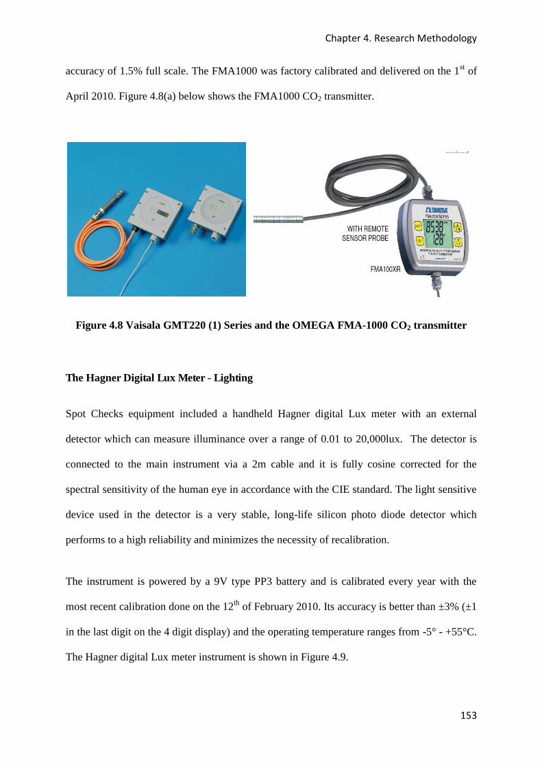
Chapter 4. Research Methodology
153
accuracy of 1.5% full scale. The FMA1000 was factory calibrated and delivered on the 1st of
April 2010. Figure 4.8(a) below shows the FMA1000 CO2 transmitter.
Figure 4.8 Vaisala GMT220 (1) Series and the OMEGA FMA-1000 CO2 transmitter
The Hagner Digital Lux Meter - Lighting
Spot Checks equipment included a handheld Hagner digital Lux meter with an external
detector which can measure illuminance over a range of 0.01 to 20,000lux. The detector is
connected to the main instrument via a 2m cable and it is fully cosine corrected for the
spectral sensitivity of the human eye in accordance with the CIE standard. The light sensitive
device used in the detector is a very stable, long-life silicon photo diode detector which
performs to a high reliability and minimizes the necessity of recalibration.
The instrument is powered by a 9V type PP3 battery and is calibrated every year with the
most recent calibration done on the 12th of February 2010. Its accuracy is better than ±3% (±1
in the last digit on the 4 digit display) and the operating temperature ranges from -5° - +55°C.
The Hagner digital Lux meter instrument is shown in Figure 4.9.
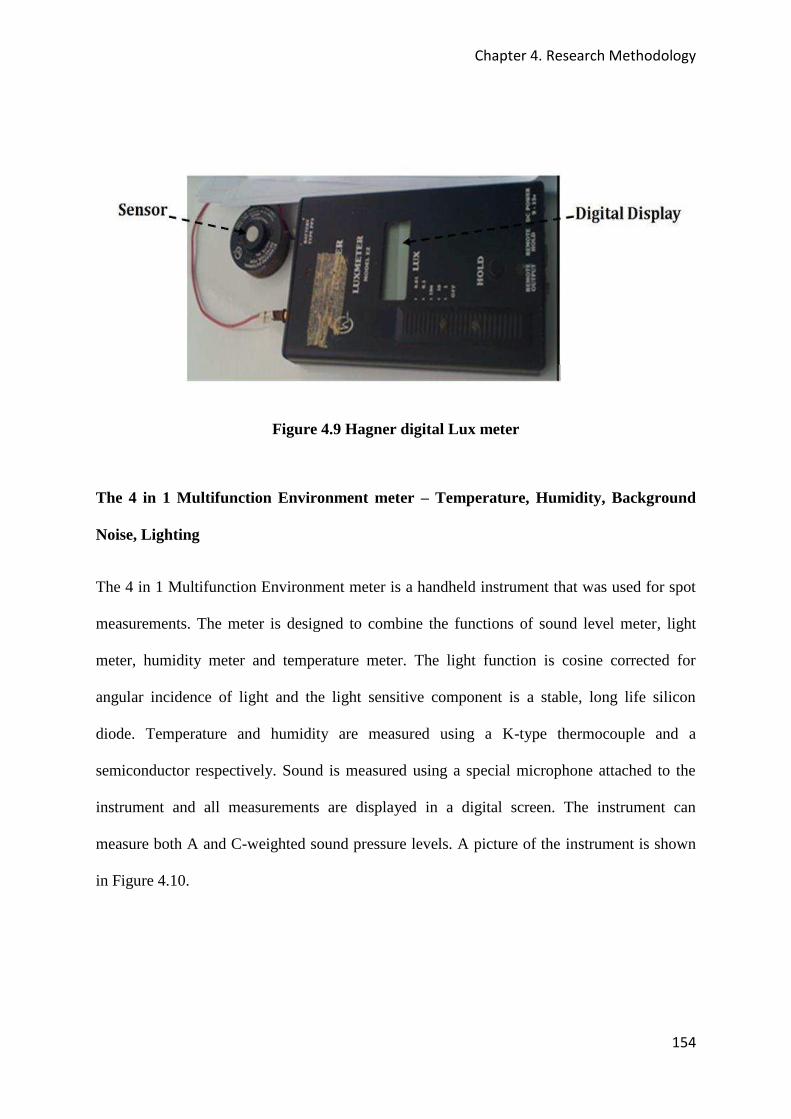
Chapter 4. Research Methodology
154
Figure 4.9 Hagner digital Lux meter
The 4 in 1 Multifunction Environment meter – Temperature, Humidity, Background
Noise, Lighting
The 4 in 1 Multifunction Environment meter is a handheld instrument that was used for spot
measurements. The meter is designed to combine the functions of sound level meter, light
meter, humidity meter and temperature meter. The light function is cosine corrected for
angular incidence of light and the light sensitive component is a stable, long life silicon
diode. Temperature and humidity are measured using a K-type thermocouple and a
semiconductor respectively. Sound is measured using a special microphone attached to the
instrument and all measurements are displayed in a digital screen. The instrument can
measure both A and C-weighted sound pressure levels. A picture of the instrument is shown
in Figure 4.10.

Chapter 4. Research Methodology
155
Figure 4.10 The 4 in 1 Multifunction Environment Meter
Table 4.4 shows some of the specifications of the instrument.
Table 4.4 Specifications of the 4 in 1 Environment Meter
Sound Lux RH % Temp Range 35-130dB 0~20,000
25~95%
-20~+750°C
Resolution 0.1dB
0.01 Lux
0.1%
0.1°C
Accuracy ±3.5dB
±5%
±5%RH
±3%Rdg +2°
The Humidity and Temperature Probe meter
The Humidity and Temperature Probe meter is a low cost handheld instrument that acted as
back up during spot measurements. The main features of the instrument include:
Rugged thermo-hygrometer with integral probe for convenient one-hand operation;
Fast response time and quality performance;
Illuminated LCD screen;
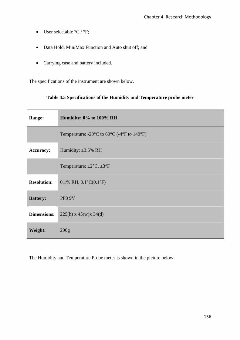
Chapter 4. Research Methodology
156
User selectable °C / °F;
Data Hold, Min/Max Function and Auto shut off; and
Carrying case and battery included.
The specifications of the instrument are shown below.
Table 4.5 Specifications of the Humidity and Temperature probe meter
Range: Humidity: 0% to 100% RH
Temperature: -20°C to 60°C (-4°F to 140°F)
Accuracy: Humidity: ±3.5% RH
Temperature: ±2°C, ±3°F
Resolution: 0.1% RH, 0.1°C(0.1°F)
Battery: PP3 9V
Dimensions: 225(h) x 45(w)x 34(d)
Weight: 200g
The Humidity and Temperature Probe meter is shown in the picture below:
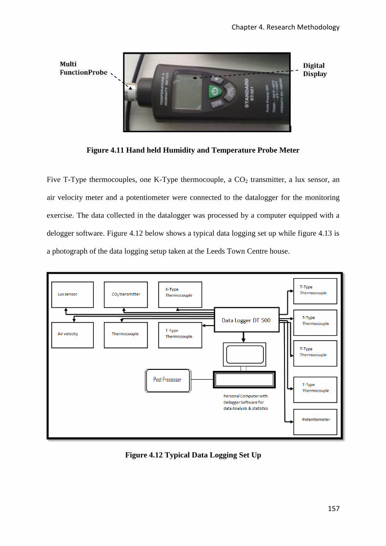
Chapter 4. Research Methodology
157
Figure 4.11 Hand held Humidity and Temperature Probe Meter
Five T-Type thermocouples, one K-Type thermocouple, a CO2 transmitter, a lux sensor, an
air velocity meter and a potentiometer were connected to the datalogger for the monitoring
exercise. The data collected in the datalogger was processed by a computer equipped with a
delogger software. Figure 4.12 below shows a typical data logging set up while figure 4.13 is
a photograph of the data logging setup taken at the Leeds Town Centre house.
Figure 4.12 Typical Data Logging Set Up
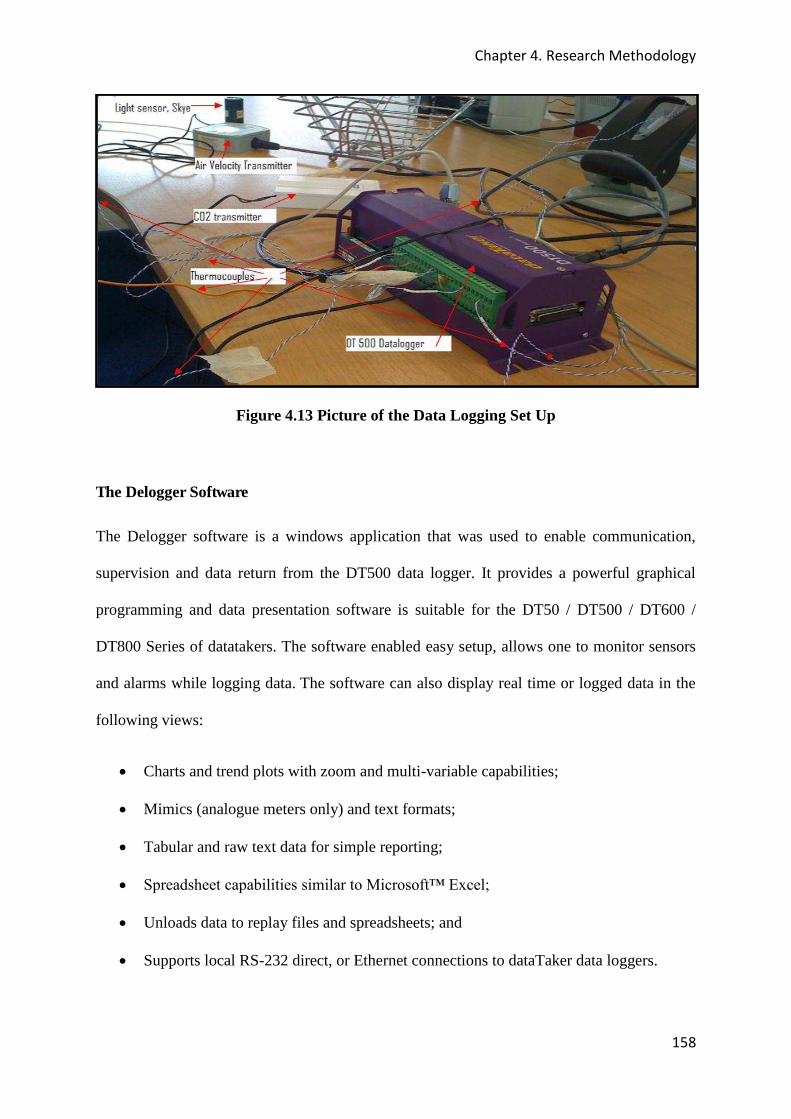
Chapter 4. Research Methodology
158
Figure 4.13 Picture of the Data Logging Set Up
The Delogger Software
The Delogger software is a windows application that was used to enable communication,
supervision and data return from the DT500 data logger. It provides a powerful graphical
programming and data presentation software is suitable for the DT50 / DT500 / DT600 /
DT800 Series of datatakers. The software enabled easy setup, allows one to monitor sensors
and alarms while logging data. The software can also display real time or logged data in the
following views:
Charts and trend plots with zoom and multi-variable capabilities;
Mimics (analogue meters only) and text formats;
Tabular and raw text data for simple reporting;
Spreadsheet capabilities similar to Microsoft™ Excel;
Unloads data to replay files and spreadsheets; and
Supports local RS-232 direct, or Ethernet connections to dataTaker data loggers.
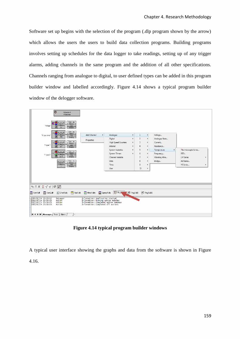
Chapter 4. Research Methodology
159
Software set up begins with the selection of the program (.dlp program shown by the arrow)
which allows the users the users to build data collection programs. Building programs
involves setting up schedules for the data logger to take readings, setting up of any trigger
alarms, adding channels in the same program and the addition of all other specifications.
Channels ranging from analogue to digital, to user defined types can be added in this program
builder window and labelled accordingly. Figure 4.14 shows a typical program builder
window of the delogger software.
Figure 4.14 typical program builder windows
A typical user interface showing the graphs and data from the software is shown in Figure
4.16.
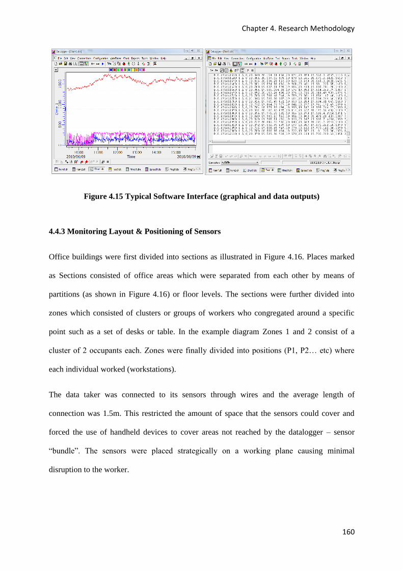
Chapter 4. Research Methodology
160
Figure 4.15 Typical Software Interface (graphical and data outputs)
4.4.3 Monitoring Layout & Positioning of Sensors
Office buildings were first divided into sections as illustrated in Figure 4.16. Places marked
as Sections consisted of office areas which were separated from each other by means of
partitions (as shown in Figure 4.16) or floor levels. The sections were further divided into
zones which consisted of clusters or groups of workers who congregated around a specific
point such as a set of desks or table. In the example diagram Zones 1 and 2 consist of a
cluster of 2 occupants each. Zones were finally divided into positions (P1, P2… etc) where
each individual worked (workstations).
The data taker was connected to its sensors through wires and the average length of
connection was 1.5m. This restricted the amount of space that the sensors could cover and
forced the use of handheld devices to cover areas not reached by the datalogger – sensor
“bundle”. The sensors were placed strategically on a working plane causing minimal
disruption to the worker.

Chapter 4. Research Methodology
161
Figure 4.16 Typical Office Divided into Sections, Zones and Positions.
Some of the thermocouples were placed at different heights above floor level in order to help
check for the presence of vertical temperature differences within the occupied space. A
typical data collection arrangement on a working plane is illustrated in Figure 4.17.
Figure 4.17 Data Collection set up on a Working Plane (Not exact layout)

Chapter 4. Research Methodology
162
The arrangement shown in Figure 4.17 was put into operation for the duration of the day and
repeated in another Zone the following day. This was complemented with spot checks in
order to ensure readings for various positions could be compared and a significant amount of
time could be saved.
Chapter 5. Results and Tool Evaluation
163
5. Results and Tool Evaluation
5.1 CASE STUDY 1: LEEDS TOWN CENTRE HOUSE
The office studied comprises modern facilities on the top floor (6th floor) of Town centre
House, Merrion Shopping Complex, at Leeds City Centre. The office is a light and airy open
plan office. It is split into sections with a reception, bespoke meeting rooms, kitchenette or
breakout areas linking the two areas. The elevated position of the building benefits the office
from daylighting as well as providing excellent views across Leeds. The building is served by
state of the art VRF cooling and heating system which incorporates heat recovery. This newly
clad building has increased levels of insulation and reduced air leakage. It boasts a striking
Yorkshire Stone façade, energy efficient passenger lifts, 24 hour CCTV security and Office
Hours commissionaire.
About 1,100 car parking spaces are available within the Merrion Shopping centre. The
building is fitted with LG7 (CIBSE, 2006) compliant Drop Rod Lighting System which uses
a Passive infra-red (PIR) lighting system which automatically switches off lights where no
movement is detected. Lights also adjust to the level of natural lighting entering the building
thereby maintaining adequate light levels throughout a working day. One section (Section A)
of the building is currently predominantly occupied by 8 people whilst the other (Section B)
is occupied by 25 people. The sections were further split into monitoring zones, three in
section A and 5 in section B.

Chapter 5. Results and Tool Evaluation
164
The total floor area of the office occupied by the 33 respondents was 370 m2 and the floor to
ceiling height is 2.9m. The office was occupied by mostly by white-collar workers consisting
of engineers and designers. Most of them performed sedentary work such as typing, filing,
drawing, telephone conversations and they wore light office clothing. It is medium furnished
and has several workstations with consisting of drawer desks and computers and filing
cabinets at the edges of the occupied space along the walls. The HVAC equipment is serviced
every three months by the supplier and had been serviced 6 days before the data collection
exercise was carried out. A more detailed description of some of the features of the building
and its activities is given in the assessment sheet presented in Figure 5.1.
Figure 5.1 Project and Building Data – Town Centre House - Leeds

Chapter 5. Results and Tool Evaluation
165
The weather conditions for the Leeds City Centre area during the three survey days were
obtained from the UK metoffice (Met Office, 2010) and weather underground (Weather
Underground, 2009) websites. The weather data is summarised in Table 5.1.
Table 5.1 Weather in Leeds during Data Collection, Source - Weather Underground
(Weather Underground, 2009)
Date Weather summary
09 June 2010 Av. ta = 11 ; Av. tdp = 11; Av. RH = 100; Partially Cloudy, midday-
afternoon, fog
10 June 2010 Av. ta = 10 ; Av. tdp = 10; Av. RH = 98; Partially Cloudy, midday-
afternoon, drizzle
11 June 2010 Av. ta = 12 ; Av. tdp = 9; Av. RH = 81; Scattered Clouds for most of the
day
5.1.1 Thermal Comfort Assessment
The sixth floor space of the Leeds Town centre house was divided into 2 Sections and 8
Zones as described in section 5.2.1 and each zone represented an occupied area (cluster of
occupants) with a unique microclimate. A full day was dedicated for the preparation of
equipment as explained in chapter 4 and another day was also dedicated for data collection in
each section of the office. An extra day was allocated for additional tests such as the
overnight logging of temperature and CO2.
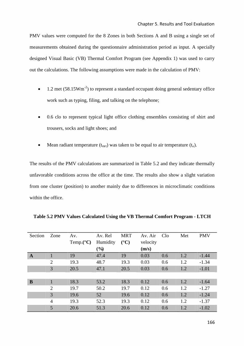
Chapter 5. Results and Tool Evaluation
166
PMV values were computed for the 8 Zones in both Sections A and B using a single set of
measurements obtained during the questionnaire administration period as input. A specially
designed Visual Basic (VB) Thermal Comfort Program (see Appendix 1) was used to carry
out the calculations. The following assumptions were made in the calculation of PMV:
1.2 met (58.15Wm-2) to represent a standard occupant doing general sedentary office
work such as typing, filing, and talking on the telephone;
0.6 clo to represent typical light office clothing ensembles consisting of shirt and
trousers, socks and light shoes; and
Mean radiant temperature (tmrt) was taken to be equal to air temperature (ta).
The results of the PMV calculations are summarized in Table 5.2 and they indicate thermally
unfavorable conditions across the office at the time. The results also show a slight variation
from one cluster (position) to another mainly due to differences in microclimatic conditions
within the office.
Table 5.2 PMV Values Calculated Using the VB Thermal Comfort Program - LTCH
Section Zone Av. Temp.(°C)
Av. Rel Humidity (%)
MRT (°C)
Av. Air velocity (m/s)
Clo Met PMV
A 1 19 47.4 19 0.03 0.6 1.2 -1.44 2 19.3 48.7 19.3 0.03 0.6 1.2 -1.34 3 20.5 47.1 20.5 0.03 0.6 1.2 -1.01 B 1 18.3 53.2 18.3 0.12 0.6 1.2 -1.64 2 19.7 50.2 19.7 0.12 0.6 1.2 -1.27 3 19.6 52 19.6 0.12 0.6 1.2 -1.24 4 19.3 52.3 19.3 0.12 0.6 1.2 -1.37 5 20.6 51.3 20.6 0.12 0.6 1.2 -1.02
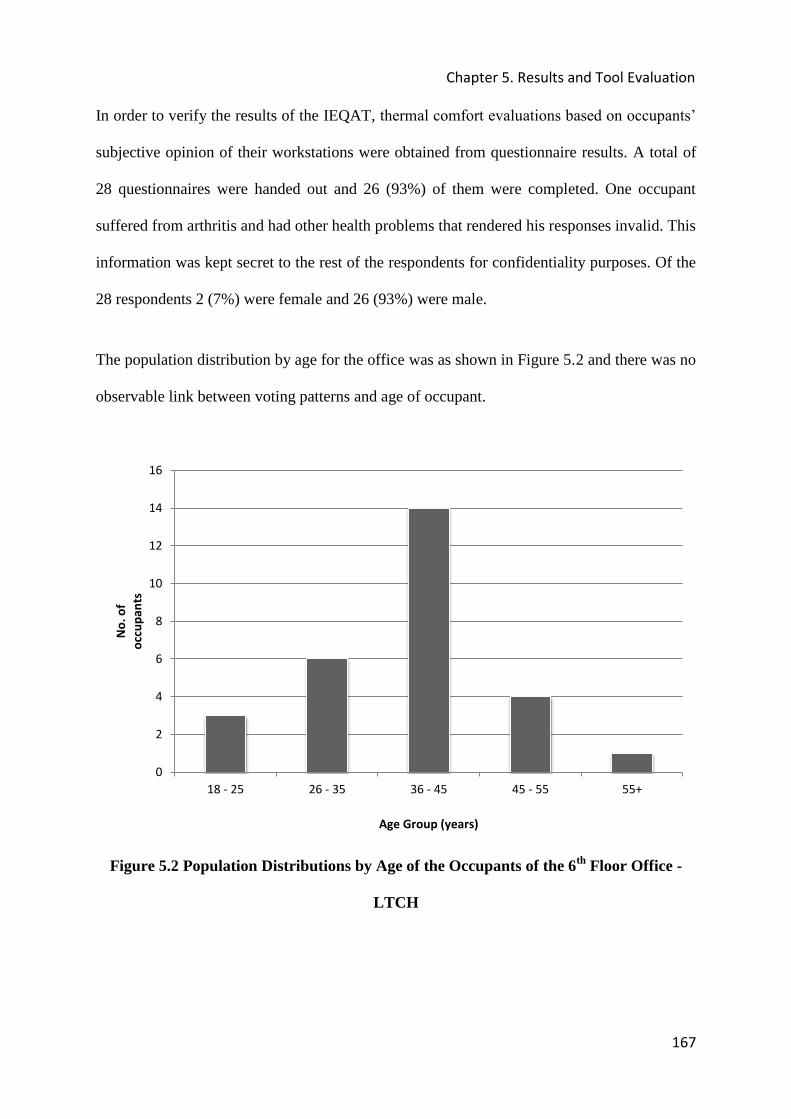
Chapter 5. Results and Tool Evaluation
167
In order to verify the results of the IEQAT, thermal comfort evaluations based on occupants’
subjective opinion of their workstations were obtained from questionnaire results. A total of
28 questionnaires were handed out and 26 (93%) of them were completed. One occupant
suffered from arthritis and had other health problems that rendered his responses invalid. This
information was kept secret to the rest of the respondents for confidentiality purposes. Of the
28 respondents 2 (7%) were female and 26 (93%) were male.
The population distribution by age for the office was as shown in Figure 5.2 and there was no
observable link between voting patterns and age of occupant.
Figure 5.2 Population Distributions by Age of the Occupants of the 6th Floor Office -
LTCH
0
2
4
6
8
10
12
14
16
18 - 25 26 - 35 36 - 45 45 - 55 55+
No
. o
f
occ
up
an
ts
Age Group (years)
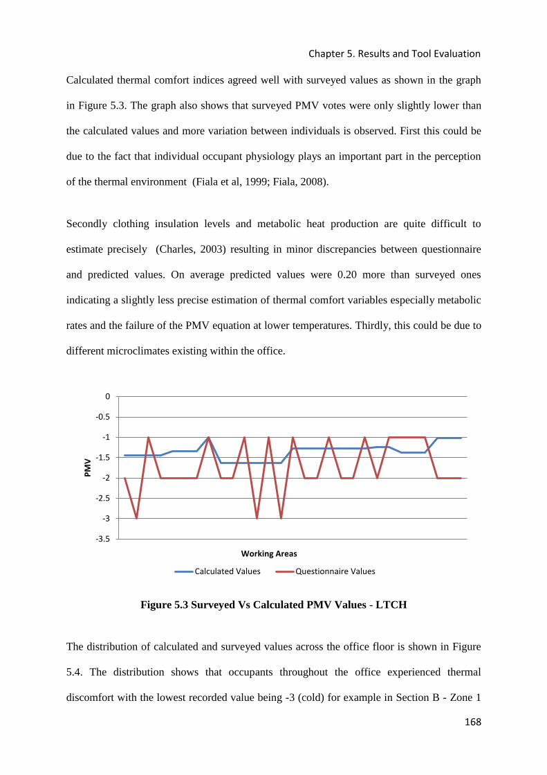
Chapter 5. Results and Tool Evaluation
168
Calculated thermal comfort indices agreed well with surveyed values as shown in the graph
in Figure 5.3. The graph also shows that surveyed PMV votes were only slightly lower than
the calculated values and more variation between individuals is observed. First this could be
due to the fact that individual occupant physiology plays an important part in the perception
of the thermal environment (Fiala et al, 1999; Fiala, 2008).
Secondly clothing insulation levels and metabolic heat production are quite difficult to
estimate precisely (Charles, 2003) resulting in minor discrepancies between questionnaire
and predicted values. On average predicted values were 0.20 more than surveyed ones
indicating a slightly less precise estimation of thermal comfort variables especially metabolic
rates and the failure of the PMV equation at lower temperatures. Thirdly, this could be due to
different microclimates existing within the office.
Figure 5.3 Surveyed Vs Calculated PMV Values - LTCH
The distribution of calculated and surveyed values across the office floor is shown in Figure
5.4. The distribution shows that occupants throughout the office experienced thermal
discomfort with the lowest recorded value being -3 (cold) for example in Section B - Zone 1
-3.5
-3
-2.5
-2
-1.5
-1
-0.5
0
PM
V
Working Areas
Calculated Values Questionnaire Values
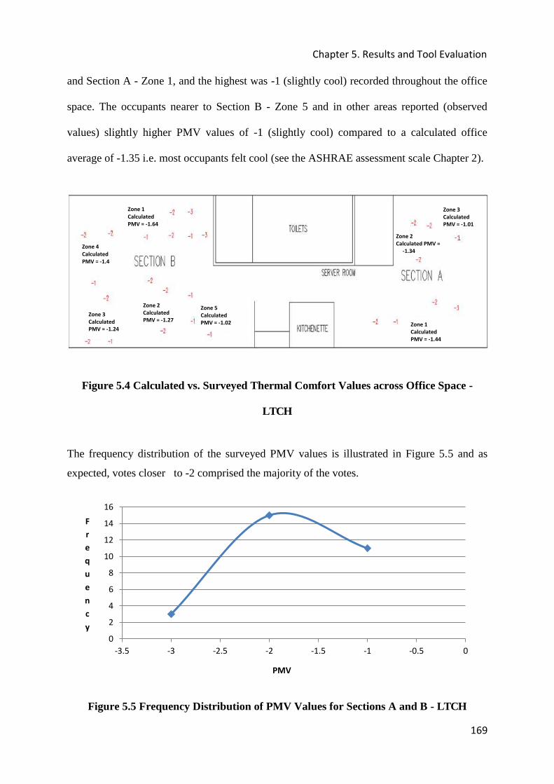
Chapter 5. Results and Tool Evaluation
169
and Section A - Zone 1, and the highest was -1 (slightly cool) recorded throughout the office
space. The occupants nearer to Section B - Zone 5 and in other areas reported (observed
values) slightly higher PMV values of -1 (slightly cool) compared to a calculated office
average of -1.35 i.e. most occupants felt cool (see the ASHRAE assessment scale Chapter 2).
Figure 5.4 Calculated vs. Surveyed Thermal Comfort Values across Office Space -
LTCH
The frequency distribution of the surveyed PMV values is illustrated in Figure 5.5 and as
expected, votes closer to -2 comprised the majority of the votes.
Figure 5.5 Frequency Distribution of PMV Values for Sections A and B - LTCH
0
2
4
6
8
10
12
14
16
-3.5 -3 -2.5 -2 -1.5 -1 -0.5 0
F
r
e
q
u
e
n
c
y
PMV
Zone 4
Calculated
PMV = -1.4
Zone 1
Calculated
PMV = -1.64
Zone 3
Calculated
PMV = -1.24
Zone 2
Calculated
PMV = -1.27
Zone 5
Calculated
PMV = -1.02
Zone 3
Calculated
PMV = -1.01
Zone 2
Calculated PMV =
-1.34
Zone 1
Calculated
PMV = -1.44
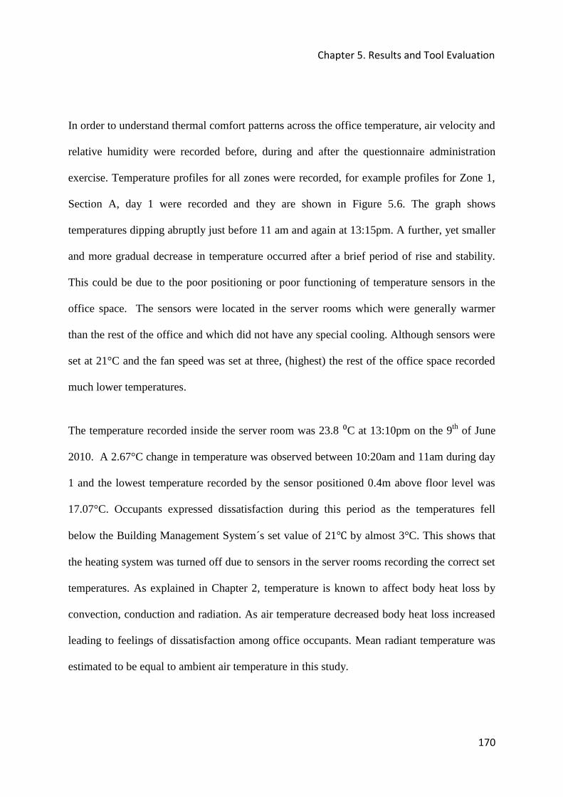
Chapter 5. Results and Tool Evaluation
170
In order to understand thermal comfort patterns across the office temperature, air velocity and
relative humidity were recorded before, during and after the questionnaire administration
exercise. Temperature profiles for all zones were recorded, for example profiles for Zone 1,
Section A, day 1 were recorded and they are shown in Figure 5.6. The graph shows
temperatures dipping abruptly just before 11 am and again at 13:15pm. A further, yet smaller
and more gradual decrease in temperature occurred after a brief period of rise and stability.
This could be due to the poor positioning or poor functioning of temperature sensors in the
office space. The sensors were located in the server rooms which were generally warmer
than the rest of the office and which did not have any special cooling. Although sensors were
set at 21°C and the fan speed was set at three, (highest) the rest of the office space recorded
much lower temperatures.
The temperature recorded inside the server room was 23.8 びC at 13:10pm on the 9th of June
2010. A 2.67°C change in temperature was observed between 10:20am and 11am during day
1 and the lowest temperature recorded by the sensor positioned 0.4m above floor level was
17.07°C. Occupants expressed dissatisfaction during this period as the temperatures fell
below the Building Management System´s set value of 21襖 by almost 3°C. This shows that
the heating system was turned off due to sensors in the server rooms recording the correct set
temperatures. As explained in Chapter 2, temperature is known to affect body heat loss by
convection, conduction and radiation. As air temperature decreased body heat loss increased
leading to feelings of dissatisfaction among office occupants. Mean radiant temperature was
estimated to be equal to ambient air temperature in this study.
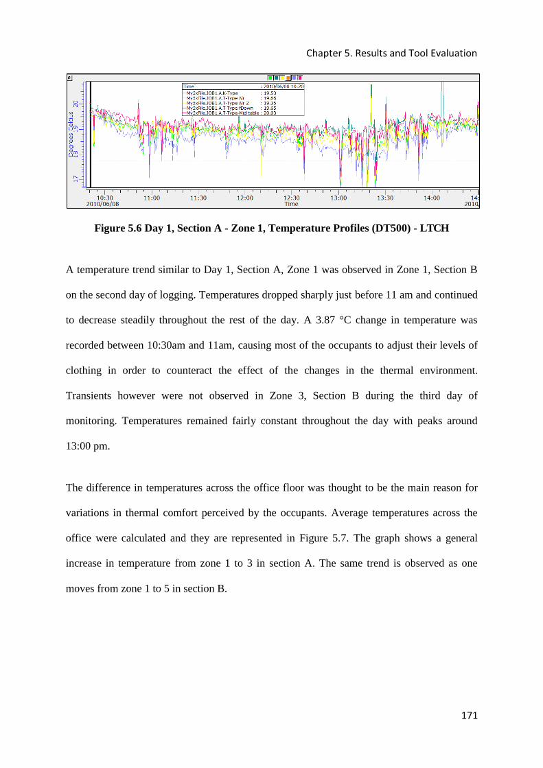
Chapter 5. Results and Tool Evaluation
171
Figure 5.6 Day 1, Section A - Zone 1, Temperature Profiles (DT500) - LTCH
A temperature trend similar to Day 1, Section A, Zone 1 was observed in Zone 1, Section B
on the second day of logging. Temperatures dropped sharply just before 11 am and continued
to decrease steadily throughout the rest of the day. A 3.87 °C change in temperature was
recorded between 10:30am and 11am, causing most of the occupants to adjust their levels of
clothing in order to counteract the effect of the changes in the thermal environment.
Transients however were not observed in Zone 3, Section B during the third day of
monitoring. Temperatures remained fairly constant throughout the day with peaks around
13:00 pm.
The difference in temperatures across the office floor was thought to be the main reason for
variations in thermal comfort perceived by the occupants. Average temperatures across the
office were calculated and they are represented in Figure 5.7. The graph shows a general
increase in temperature from zone 1 to 3 in section A. The same trend is observed as one
moves from zone 1 to 5 in section B.

Chapter 5. Results and Tool Evaluation
172
Figure 5.7 Recorded Mean Temperatures - LTCH
Survey results also showed that cold draughts were felt by 17 of the 26 occupants during the
survey time. It has been established from literature that air movement produces a cooling
effect on the skin and increased air velocities can produce a feeling of comfort even at
increased temperatures (Fanger, 1973; Charles, 2003). However sudden changes in air
velocities could result in feelings of draught which may lead to local discomfort especially at
low temperatures. However upon investigation air velocities were only restricted to isolated
peaks of less than 0.2m/s and sudden variations in temperature was thought to be the main
reason why most occupants mentioned cold draughts.
Seven of the 17 occupants also recorded local discomfort due to vertical temperature
differences. Vertical air temperature differences were also investigated and found to be less
than 1°C. In order to check the presence of vertical temperature difference thermocouples
were placed at different heights above the floor level and in section A, Zone 1 a vertical air
temperature difference was observed as shown in Figure 5.8. The high number occupants
dissatisfied with vertical temperature difference could be explained by the fact that the air
15
16
17
18
19
20
21
Zone 1,
Section A
Zone 2,
Section A
Zone 3,
Section A
Zone 1,
Section B
Zone 2,
Section B
Zone 3,
Section B
Zone 4,
Section B
Zone 5,
Section B
Te
mp
era
ture
(°C
)
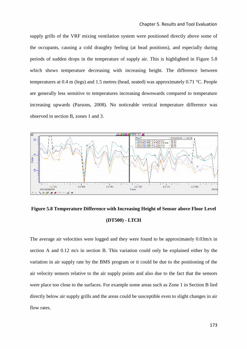
Chapter 5. Results and Tool Evaluation
173
supply grills of the VRF mixing ventilation system were positioned directly above some of
the occupants, causing a cold draughty feeling (at head positions), and especially during
periods of sudden drops in the temperature of supply air. This is highlighted in Figure 5.8
which shows temperature decreasing with increasing height. The difference between
temperatures at 0.4 m (legs) and 1.5 metres (head, seated) was approximately 0.71 °C. People
are generally less sensitive to temperatures increasing downwards compared to temperature
increasing upwards (Parsons, 2008). No noticeable vertical temperature difference was
observed in section B, zones 1 and 3.
Figure 5.8 Temperature Difference with Increasing Height of Sensor above Floor Level
(DT500) - LTCH
The average air velocities were logged and they were found to be approximately 0.03m/s in
section A and 0.12 m/s in section B. This variation could only be explained either by the
variation in air supply rate by the BMS program or it could be due to the positioning of the
air velocity sensors relative to the air supply points and also due to the fact that the sensors
were place too close to the surfaces. For example some areas such as Zone 1 in Section B lied
directly below air supply grills and the areas could be susceptible even to slight changes in air
flow rates.

Chapter 5. Results and Tool Evaluation
174
Irregular patterns of air velocities were observed during office hours at the Town Centre
House. Results for zone 1, section B (Figure 5.9) show an abrupt increase in air velocities just
before 11am (survey period) and corresponding abrupt decreases in temperature as the BMS
responded either to changes in the program or as a result of stimulation of sensors.
Figure 5.9 Day Two, Section B - Zone 1, Recorded Air Velocities (DT500) - LTCH
The prevalence of local discomfort factors felt by occupants are summarised in Table 5.3.
Table 5.3 Prevalence of local discomfort factors experienced by occupants
Symptom No. of occupants experienced symptom
Draughts 17
Vertical Air Temperature Difference 7
Cold Surfaces 0
Asymmetrical radiant heat e.g. radiators
or other heat emitters
0

Chapter 5. Results and Tool Evaluation
175
5.1.2 Indoor Air Quality Assessment
CO2 concentrations were used as indicators of indoor air pollution since it was assumed that
bio effluents were major contributors of pollution in the indoor environment. Figure 5.10
shows a typical CO2 concentration profile observed during the survey period.
Figure 5.10 CO2 Concentration Profile, Day 3 (DT500) - LTCH
During the survey period the average measured CO2 concentration was 800ppm, 370ppm
above outdoor concentration. A base level CO2 concentration of 429 ppm was used and this
value was obtained from average concentration during night time. This value was used to
calculate PDIAQ using equation 3.16 (Chapter 3). The number of people satisfied (1- PDIAQ)
with air quality was estimated at 87.5% (equation 3.20). Surveyed values of number of
people satisfied with IAQ were also estimated from questionnaire responses. The mean
surveyed acceptance of IAQ was 84.6% (SD 13.47). The minimum value was 62.5% while
the maximum was 100% (maximum acceptability). The average 84.6% is very close to the
calculated value of 87.5% (Figure 5.11) hence this method could be used to calculate the
quality of indoor air where bio effluents are the main pollutants.

Chapter 5. Results and Tool Evaluation
176
Figure 5.11 Surveyed Vs Predicted IAQ Perception in the Office - LTCH
The prevalence of The Sick Building Syndrome (SBS) symptoms was investigated using the
questionnaire. Only five occupants expressed “blocked nose” during the survey period and
their responses were about halfway on the VAS (see questionnaire) indicating that this
problem was not “very serious”.
5.1.3 Acoustic Comfort Assessment
Critical listening was carried out to determine the nature of background noise. Most noise
was in speech related and in the form of conversations, coughing and sneezing. Walking,
typing, filing, drawers opening and closing were also quite frequent. Continuous background
noise from servers and HVAC equipment was approximately 65.5 dBA inside the server
room. The two far ends of the office recorded about 34.5 dBA and 39.4 dBA in section A and
B respectively, in the absence of conversations or any human related noise.
The level of satisfaction with the acoustic environment was calculated using equations 3.21
to 3.24 and following the procedures recommended in Chapter 3. The calculated level of
satisfaction with the acoustic environment ranged from 59.3% for those near the reception
area to 96.8% for those furthest away from the reception and server room areas. Surveyed
0
20
40
60
80
100 %
Sa
tisf
ied
Position in Office
Predicted Surveyed

Chapter 5. Results and Tool Evaluation
177
results showed a close agreement with calculated values (correlation coefficient = 0.69) as
illustrated in Figure 5.12.
Figure 5.12 Surveyed Vs Calculated Acoustic Comfort values - LTCH
5.1.4 Lighting Quality Assessment
The average horizontal illumination measured on a working plane at each zone ranged from
416 to 2065 lux. These values were measured using logging apparatus and handheld
instruments (see Hagner digital Lux meter, Figure 4.23). The skye lux sensor produced
measurements that correlated well with handheld instruments at all illumination levels.
Typical logged horizontal illumination levels are shown in Figure 5.13. The graph shows
irregular patterns of illumination during the morning period (9:30 – 10:30 AM) due to cloud
movement and a fairly steady and high illumination during the rest of the day (due to clearer
skies). Lighting within the office was designed to adjust according to the amount of daylight
received and hence the average illuminance levels were above the design value of 500 lux for
most of the times.
0
20
40
60
80
100
% s
ati
sfie
d
Surveyed Values Calculated Values
Chapter 5. Results and Tool Evaluation
178
Figure 5.13 Day 2, Section A, Illuminance (DT500) - LTCH
Lighting quality (Lindex) in the office was calculated using equation 3.25 (Chapter 3).
Comparison of surveyed and calculated lighting acceptance values showed that the two
methods are in fairly good agreement with some observed IEQ results showing large
variations between cases. The main problem associated with this is that most questions on
lighting acceptance are vague hence they do not produce precise results.
This could be mainly because lighting acceptance is not necessarily proportional to the
amount of light received, but rather relies on many other aspects that have not been taken into
account. For example at higher illuminance levels some people may feel discomfort due to
too much light for their requirements being received, or due to the presence of glare. The
other problem is that VAS scales simply describe acceptability of the lighting environment
but do not relate much to the “amount of light” received on a working plane. Figure 5.14 is a
graph that compares model and surveyed results.
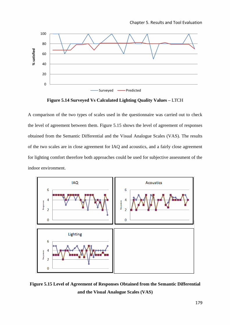
Chapter 5. Results and Tool Evaluation
179
Figure 5.14 Surveyed Vs Calculated Lighting Quality Values – LTCH
A comparison of the two types of scales used in the questionnaire was carried out to check
the level of agreement between them. Figure 5.15 shows the level of agreement of responses
obtained from the Semantic Differential and the Visual Analogue Scales (VAS). The results
of the two scales are in close agreement for IAQ and acoustics, and a fairly close agreement
for lighting comfort therefore both approaches could be used for subjective assessment of the
indoor environment.
Figure 5.15 Level of Agreement of Responses Obtained from the Semantic Differential
and the Visual Analogue Scales (VAS)
0
20
40
60
80
100 %
sa
tisf
ied
Surveyed Predicted

Chapter 5. Results and Tool Evaluation
180
5.1.5 Indoor Environment Quality Assessment
A picture of the indoor environment showing the design and furniture level was taken at the
end of the survey day and it is shown in Figure 5.16.
Figure 5.16 Picture of Indoor Environment - LTCH
Using equation (3.30) provisional IEQ (IEQindex) values were calculated and the results of
descriptive statistics showed a standard deviation of 7.05 and a sample mean of 74.64. The
minimum and maximum values were 62.92 and 85.01 respectively. The sample mean shows
that occupants found the indoor environment generally “acceptable” despite variations in
thermal comfort opinions across the office floor. Model calculated IEQ results were
compared to questionnaire results in Figure 5.17 and they showed agreements to within 10%.
The results also showed similar “general trends” across the office floor space. The AHP
generated IEQ was used to check the validity of linear models as IEQ assessment tools for
office buildings in the UK.
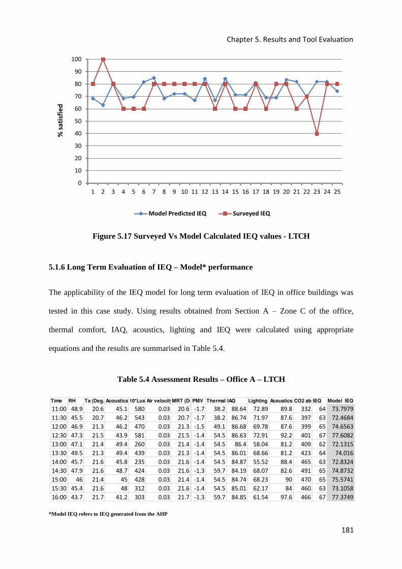
Chapter 5. Results and Tool Evaluation
181
Figure 5.17 Surveyed Vs Model Calculated IEQ values - LTCH
5.1.6 Long Term Evaluation of IEQ – Model* performance
The applicability of the IEQ model for long term evaluation of IEQ in office buildings was
tested in this case study. Using results obtained from Section A – Zone C of the office,
thermal comfort, IAQ, acoustics, lighting and IEQ were calculated using appropriate
equations and the results are summarised in Table 5.4.
Table 5.4 Assessment Results – Office A – LTCH
*Model IEQ refers to IEQ generated from the AHP
0
10
20
30
40
50
60
70
80
90
100
1 2 3 4 5 6 7 8 9 10 11 12 13 14 15 16 17 18 19 20 21 22 23 24 25
% s
ati
sfie
d
Model Predicted IEQ Surveyed IEQ
Time RH Ta (Deg. Acoustics 10*Lux Air velocityMRT (DeCPMV Thermal CIAQ Lighting Acoustics CO2 aboIEQ Model IEQ
11:00 48.9 20.6 45.1 580 0.03 20.6 -1.7 38.2 88.64 72.89 89.8 332 64 73.7979
11:30 45.5 20.7 46.2 543 0.03 20.7 -1.7 38.2 86.74 71.97 87.6 397 63 72.4684
12:00 46.9 21.3 46.2 470 0.03 21.3 -1.5 49.1 86.68 69.78 87.6 399 65 74.6563
12:30 47.3 21.5 43.9 581 0.03 21.5 -1.4 54.5 86.63 72.91 92.2 401 67 77.6082
13:00 47.1 21.4 49.4 260 0.03 21.4 -1.4 54.5 86.4 58.04 81.2 409 62 72.1315
13:30 49.5 21.3 49.4 439 0.03 21.3 -1.4 54.5 86.01 68.66 81.2 423 64 74.016
14:00 45.7 21.6 45.8 235 0.03 21.6 -1.4 54.5 84.87 55.52 88.4 465 63 72.8324
14:30 47.9 21.6 48.7 424 0.03 21.6 -1.3 59.7 84.19 68.07 82.6 491 65 74.8732
15:00 46 21.4 45 428 0.03 21.4 -1.4 54.5 84.74 68.23 90 470 65 75.5741
15:30 45.4 21.6 48 312 0.03 21.6 -1.4 54.5 85.01 62.17 84 460 63 73.1058
16:00 43.7 21.7 41.2 303 0.03 21.7 -1.3 59.7 84.85 61.54 97.6 466 67 77.3749

Chapter 5. Results and Tool Evaluation
182
Results can be produced for longer periods provided the input data has been collected over
longer periods. Forms of results presentation have been described in Chapter 3. Figure 5.18
shows the results in graphical form (line graph) since this provides a clearer picture of the
conditions likely to have been experienced during that period.
Figure 5.18 Assessment Results – Section A, Line Graph Presentation - LTCH
In order to compare IEQ with building energy performance values for the duration of the year
need to be averaged and presented as shown in Figure 5.21. A radar chart provides an
excellent pictorial comparison between the IEQ aspects and energy performance. Energy
performance of the office can be introduced into the radar chart as the sixth quantity.
0
10
20
30
40
50
60
70
80
90
100
11:00 11:30 12:00 12:30 13:00 13:30 14:00 14:30 15:00 15:30 16:00
% s
ati
sfie
d/r
ati
ng
Thermal Comfort
IAQ
Lighting
Acoustics
Model Predicted IEQ
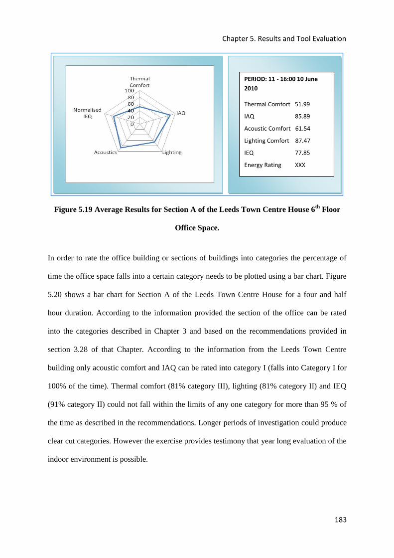
Chapter 5. Results and Tool Evaluation
183
Figure 5.19 Average Results for Section A of the Leeds Town Centre House 6th Floor
Office Space.
In order to rate the office building or sections of buildings into categories the percentage of
time the office space falls into a certain category needs to be plotted using a bar chart. Figure
5.20 shows a bar chart for Section A of the Leeds Town Centre House for a four and half
hour duration. According to the information provided the section of the office can be rated
into the categories described in Chapter 3 and based on the recommendations provided in
section 3.28 of that Chapter. According to the information from the Leeds Town Centre
building only acoustic comfort and IAQ can be rated into category I (falls into Category I for
100% of the time). Thermal comfort (81% category III), lighting (81% category II) and IEQ
(91% category II) could not fall within the limits of any one category for more than 95 % of
the time as described in the recommendations. Longer periods of investigation could produce
clear cut categories. However the exercise provides testimony that year long evaluation of the
indoor environment is possible.
PERIOD: 11 - 16:00 10 June
2010
Thermal Comfort 51.99
IAQ 85.89
Acoustic Comfort 61.54
Lighting Comfort 87.47
IEQ 77.85
Energy Rating XXX

Chapter 5. Results and Tool Evaluation
184
Figure 5.20 Percentages of time Office falls inside the limits of a Category - LTCH
Assuming that IEQ falls within Category II (74.40) for 95% (actual value is 91%) or more of
the time for section A and Category II for (74.54) for section B (> 95% of the time) and using
the methodology presented in Chapter 3 (equations 3.31 – 32), the IEQ rating for the Leeds
office is calculated as follows:
IEQindex for section A = 74.40;
Floor Area ratio = 1/3;
IEQindex for section B = 74.54;
Floor Area ratio = 2/3
5. ASSESSMENT RESULTS BAR GRAPH DISPLAY (11 - 16:00; 10 June 2010)

Chapter 5. Results and Tool Evaluation
185
IEQ rating for both sections for the survey period is given as:
荊継芸 迎欠建件券訣 噺 岷岾ばね┻ねど 抜 怠戴峇 髪 岾ばね┻のね 抜 態戴峇 噺 挿想┻ 想操┸ for the period 11AM – 4PM, on the
10th of June 2010.
5.1.7 General Considerations for the Indoor Environment
Table 5.5 Checklists for IEQ variables – Leeds Town Centre House
Sound insulation properties (material properties), pollutant levels, daylight and other lighting
factors were not available for inclusion into the results sheet of this office building.
Chapter 5. Results and Tool Evaluation
186
5.1.8 Conclusions and Lessons Learnt From the Study
The Leeds Town Centre Building case study highlights the importance of thermal comfort,
IAQ, acoustics and lighting to occupants’ perceptions of the quality of the indoor
environment. The relative importance of each of the factors depends on prevailing
microclimatic conditions hence there is need for a large number of studies to be carried out in
order to determine trends associated with different sets of indoor conditions. The offices
studied in the Leeds Town Centre House had a particularly unique set of indoor environment
conditions as shown by the summaries of logged data. This could pave way for weightings
that are based on occupant’s subjective opinions and therefore less biased models can be
produced.
The study also shows that the new IEQ methodology has great potential to be used as an
ultimate tool that can be used to assess office buildings at any stage of the design. Special
arrangements need to be made for occupants who may suffer from diseases that affect their
perceptions of comfort in the office. For example occupants who suffer from Reynaud’s
disease and arthritis were found to be particularly susceptible to cold.
Chapter 5. Results and Tool Evaluation
187
5.2 CASE STUDY 2:
MARSH, GROCHOWSKI & ASSOCIATES, NOTTINGHAM
The office studied is a naturally ventilated pre-world war II building located at Commerce
Square, Lace Market, Nottingham City Centre in the United Kingdom. The building is a
1930s open plan consisting of triple height spaces. It comprises four floors with the ground
floor comprising of meeting rooms and first floor comprises rest rooms and a kitchenette. The
second floor consists of office space that is divided into two parts with two people occupying
the first lower level section and three people occupying the second, upper level section. The
higher section of the first floor is fitted with ordinary non energy efficient (incandescent) 60
watts light bulbs and the lower of the two sections has an atrium which supplies extra natural
light.
The third and top floor is a standard office room which is naturally ventilated and occupied
by three people. The top floor office space however has blinds fitted on all windows to
prevent glare due to direct sunlight at certain times of the day. The position of the building
means it is heavily shaded by other buildings hence it benefits less from daylighting. The
heating needs of this building are served by isolated electric heaters and cooling in summer is
assisted by plug in electric fans. This building has poor levels of insulation. The main walls
consist of double brick with plaster and paint on the internal side, loose fitting single glazed
windows on a metal frame. Ventilation air is supplied through supply air vents situated at
various points within the building.
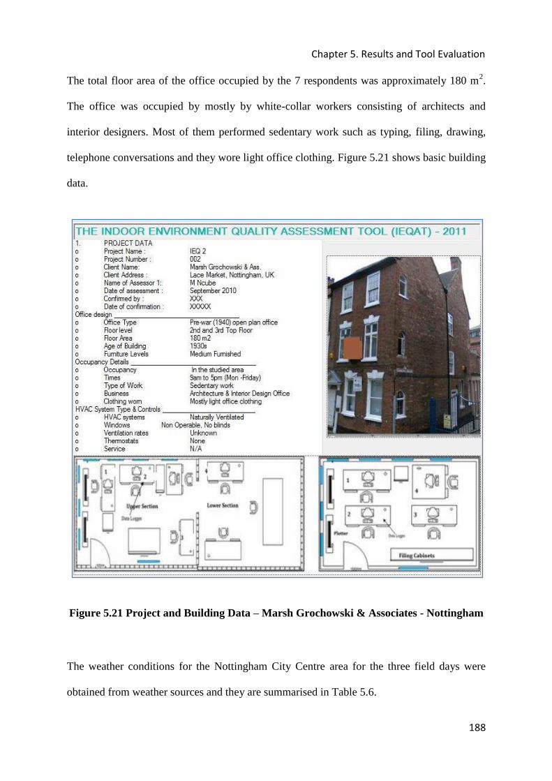
Chapter 5. Results and Tool Evaluation
188
The total floor area of the office occupied by the 7 respondents was approximately 180 m2.
The office was occupied by mostly by white-collar workers consisting of architects and
interior designers. Most of them performed sedentary work such as typing, filing, drawing,
telephone conversations and they wore light office clothing. Figure 5.21 shows basic building
data.
Figure 5.21 Project and Building Data – Marsh Grochowski & Associates - Nottingham
The weather conditions for the Nottingham City Centre area for the three field days were
obtained from weather sources and they are summarised in Table 5.6.
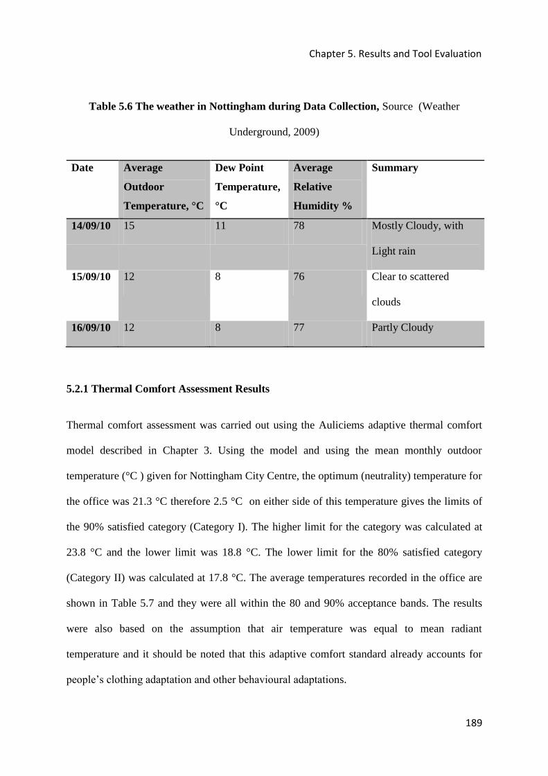
Chapter 5. Results and Tool Evaluation
189
Table 5.6 The weather in Nottingham during Data Collection, Source (Weather
Underground, 2009)
Date Average
Outdoor
Temperature, °C
Dew Point
Temperature,
°C
Average
Relative
Humidity %
Summary
14/09/10 15 11 78 Mostly Cloudy, with
Light rain
15/09/10 12 8 76 Clear to scattered
clouds
16/09/10 12 8 77 Partly Cloudy
5.2.1 Thermal Comfort Assessment Results
Thermal comfort assessment was carried out using the Auliciems adaptive thermal comfort
model described in Chapter 3. Using the model and using the mean monthly outdoor
temperature (°C ) given for Nottingham City Centre, the optimum (neutrality) temperature for
the office was 21.3 °C therefore 2.5 °C on either side of this temperature gives the limits of
the 90% satisfied category (Category I). The higher limit for the category was calculated at
23.8 °C and the lower limit was 18.8 °C. The lower limit for the 80% satisfied category
(Category II) was calculated at 17.8 °C. The average temperatures recorded in the office are
shown in Table 5.7 and they were all within the 80 and 90% acceptance bands. The results
were also based on the assumption that air temperature was equal to mean radiant
temperature and it should be noted that this adaptive comfort standard already accounts for
people’s clothing adaptation and other behavioural adaptations.

Chapter 5. Results and Tool Evaluation
190
Questionnaire results presented an opportunity to test the relationship between model results
and occupants’ evaluation of the thermal environment (the results are summarized in Figures
5.25). All healthy occupants reported feeling slightly cool as shown in Figures 5.22 and 5.23.
In the second floor the occupant in position 1 indicated that they suffer from arthritis. In the
top floor the occupant in position 6 voted PMV = -3 and they also indicated that they also
suffered from Reynaud’s disease which could have affected their perception of the indoor
environment. Those two values were rendered invalid for purposes of assessing the
performance of the model.
Using the assessment scale presented in the Questionnaire (Appendix 2) the votes slightly
cool corresponded with 85% (for median values) acceptability of the indoor thermal
environment. These results agree well with model calculated results for that building as
shown in Figure 5.25 although the model overestimates perceived thermal comfort by 2.5%
as shown in Figure 5.25. The assessment scale used in the questionnaire could however be
improved to include more choices for respondents to select. This will allow for more
variation in choices made by occupants and help indicate any variations in the indoor
microclimate from the opinions of the individuals.
Figure 5.22 Questionnaire Results for the 2nd Floor, Marsh & Grochowski Architects,
Nottingham
P4
P3
P2
P1
Slightly Cool
Slightly Cool
Slightly Cool Cool ふRW┞ミ;┌Sげゲぶ

Chapter 5. Results and Tool Evaluation
191
Figure 5.23 Questionnaire Results for the 3rd Floor, Marsh & Grochowski Architects –
Nottingham
Table 5.7 Summary of Thermal Comfort variables and calculated PMV values – MGA
Floor Position Air
Temperature
Recorded
Model
Predicted
Acceptance
Surveyed or
Questionnaire Results
Comment
2nd 1 19.5 89.5 Cool Reject
2 19.4 88.9 Slightly Cool
3 19.4 88.9 Slightly Cool
4 19.6 90.2 Slightly Cool
3rd 1 19.2 87.4 Slightly Cool
2 19.2 87.4 Cold Reject
It is important to note that occupants were observed as they made efforts to improve their
situation by adjusting their clothing, using electric heaters and taking hot drinks regularly
throughout the day. Such actions are energy intensive and they add significantly to the energy
bills in naturally ventilated buildings. As explained earlier most occupants voted 9slightly
cool: (except those with underlying health conditions) as shown in Figure 5.24.
P6
P5
Slightly Cool
Cold (Arthritis)

Chapter 5. Results and Tool Evaluation
192
Figure 5.24 Frequency distribution of PMV values for the Marsh & Grochowski
Architects, Nottingham
Figure 5.25 compares model calculated and surveyed thermal comfort results.
Figure 5.25 Model vs Questionnaire thermal comfort values for the Marsh, Grochowski
& Associates -Nottingham
0
0.5
1
1.5
2
2.5
3
3.5
4
4.5
Cold Cool Slightly Cool Netral Slightly
Warm
Warm Hot
Fre
qu
en
cy o
f V
ote
s
0
10
20
30
40
50
60
70
80
90
100
1 2 3 4
% S
ati
sfa
ctio
n
Occupant
Surveyed Model Calculated
Cat: I
Cat: II
Cat: III

Chapter 5. Results and Tool Evaluation
193
Temperature, relative humidity and air velocity were recorded throughout the survey period
as done at the Leeds office and the results are explained below. The data logger was checked
for its accuracy using a potentiometer sensor and the temperature profiles for the 3rd and 4th
floors were recorded and an example is shown in Figures 5.26.
Figure 5.26 Temperature Profile for the Top (3rd) Floor Section of the Office Building
(DT500) - MGA
Figure 5.26 show fairly constant temperatures throughout the office hours with peak daily
temperatures being recorded at 19.87ºC and minimum daily temperatures recorded at 17ºC.
Temperature drops after 6 PM (not shown) were observed mainly due to reduction in solar
gains and occupants leaving the office. Temperatures continued to fall throughout the night as
expected and gains were observed from approximately 7AM on wards as solar gains and
occupancy increased. An average temperature of 19.4 and 19.0 ºC were observed between
10:30 AM and Noon (Questionnaire Period) during survey day 1 and 2 respectively. No
noticeable vertical temperature differences were observed during the survey period. The
average temperatures taken at various locations during questionnaire administration periods
are shown in Figure 5.27. Little variation in temperatures in the 2nd floor office is observed
and a difference between minimum and maximum temperatures was 0.2°C.

Chapter 5. Results and Tool Evaluation
194
Figure 5.27 Temperature Profiles at Various Locations in the Office - MGA
Relative humidity (%) was recorded every 30 minutes between 10AM and 12:20PM using
hand held devices and the average results are summarised in Table 5.8. Higher relative
humidities were observed in the third floor probably due to the state of weather on that day.
Table 5.8 Average Relative Humidity Recorded at Various Positions in the Offices -
MGA
Section RH (%)
Position 1
RH (%)
Position 2
RH (%)
Position 3
RH (%) Position 4
2nd Floor 56.9 58.7 56.7 56.7
3rd Floor 63.0 63.0 63.0 63.0
10
12
14
16
18
20
22
P 1 2ND FLOOR P2 2ND FLOOR P3 2ND FLOOR P4 2ND FLOOR P5 3RD FLOOR P6 3RD FLOOR
Ro
om
Te
mp
era
ture
(d
eg
. C
elc
.)
Average temperatures at various positions

Chapter 5. Results and Tool Evaluation
195
Average air velocities were recorded at 0.010 m/s for most of the office hours therefore they
were recorded as “Not noticeable” air movement. Figure 5.28 shows air velocities remained
fairly constant throughout the day and a similar trend was observed in the 3rd floor.
Figure 5.28 Recorded Air Velocities – Second Floor Marsh & Grochowski Architects,
Nottingham (DT500)
Local discomfort factors such as draughts, vertical air temperature difference, between head
and feet) and cold equipment were reported by 50 percent of occupants. All occupants who
reported feeling draughty also reported vertical air temperature difference. Physical
measurements suggested otherwise because the difference in measured temperature between
head and ankles was approximately 0.22ºC. Local discomfort ratings were not measured in
this study.
5.2.2 IAQ Assessment Results
Carbon dioxide concentrations were logged and overnight concentrations were recorded at
390 ppm in the 2nd floor office with the highest recorded concentration being 1140 ppm.
During questionnaire administration the recorded average concentration was 900ppm,
therefore we can assume that the concentration of CO2 above outdoor concentration was

Chapter 5. Results and Tool Evaluation
196
510ppm. The average concentration calculated from data recorded during questionnaire
administration in the third floor was 1,100ppm while outdoor concentrations were 400ppm.
Therefore the CO2 concentration above outdoor was estimated at 700ppm.
A typical CO2 profile is shown in Figure 5.29. The graph shows the concentrations of CO2
rising steadily from around 7AM when occupancy began up to a peak around midday when
the highest number of occupants were at their workstations. There was a slight drop in
concentrations from between 1 and 3 PM as some occupants left for their lunch and a steady
rise when they returned to their workstations. The concentrations begin to fall when
occupants leave the office at the end of the day and concentrations continue to fall until they
stay constant throughout the night.
Figure 5.29 CO2 Concentrations over a 24hr Period in the Third Floor of the Office
Building (DT500) - MGA
The number of occupants satisfied with IAQ was calculated using equation 3.13 and the
results are summarised in Figure 5.30. The Figure shows discrepancies in the level of
agreement between calculated and surveyed IAQ for different positions within the office and
this could be mainly due to the fact that CO2 was measured at only one location within the
office. Again the perceived IAQ could be due to other factors such as the presence of VOCs,

Chapter 5. Results and Tool Evaluation
197
particulates, or other physical and biological agents. Signs of SBS were recorded in the office
although all occupants expressed satisfaction with the quality of the air. Dry nose and stuffy
environment was recorded by almost half of the occupants and one third expressed
dissatisfaction with level of control (the fact that windows could not be opened).
This shows that the use of CO2 concentrations to indicate the quality of the indoor
environment should be limited to environments polluted due to bio effluents only. The
method should however be used in conjunction with other methods such as the use of
ventilation rates (the dilution of pollutants approach, or the so-called ventilation for health
and comfort). The results also highlight the need to improve the precision of visual
assessment scales used in the questionnaire by adding more values so that choices are more
precise (smaller divisions).
Figure 5.30 Calculated vs. Surveyed Acceptance of IAQ - MGA
0
10
20
30
40
50
60
70
80
90
100
1 2 3 4 5 6
Acc
ep
tan
ce
Calculated Acceptance of IAQ Surveyed IAQ Acceptance
Chapter 5. Results and Tool Evaluation
198
5.23 Acoustics Comfort Assessment Results
The nature of background noise in the office was determined by critical listening.
Background noise consisted on soft music playing from a portable radio, walking, typing on
computers, filing, plotters, drawers, and isolated cases of conversations. The portable radio
was located at position 1 and a sound level meter placed at position 2 recorded 28 dBA. The
radio plus movements around the office gave a reading of 36 dBA and the highest noise
levels of 66 dBA recorded included conversations between two people and a telephone
ringing. Generally noise levels ranged from 24.4 – 54.8 dBA throughout the offices.
Calculated values for acceptance of the indoor acoustic environment were obtained from
equations described in Chapter 3. Three of the six surveyed results showed a close match
with calculated values as illustrated in Figure 5.31. It is important to note that more research
is needed to verify the acoustic comfort model suggested in this thesis and to compare it with
other models such as the Kjellberg et al and Nillson models explained in Chapter 3. Also in
areas where higher dBA values were recorded, particularly large differences between survey
and model results were observed (e.g. first two values Figure 5.31). This could also be mainly
due to the fluctuating and abrupt or short lived nature of conversation and telephone noise
within office buildings. Most importantly it is necessary that in future studies continuous
measurement of sound pressure levels including their frequencies needs to be carried out and
matched closely with times questionnaires were filled.
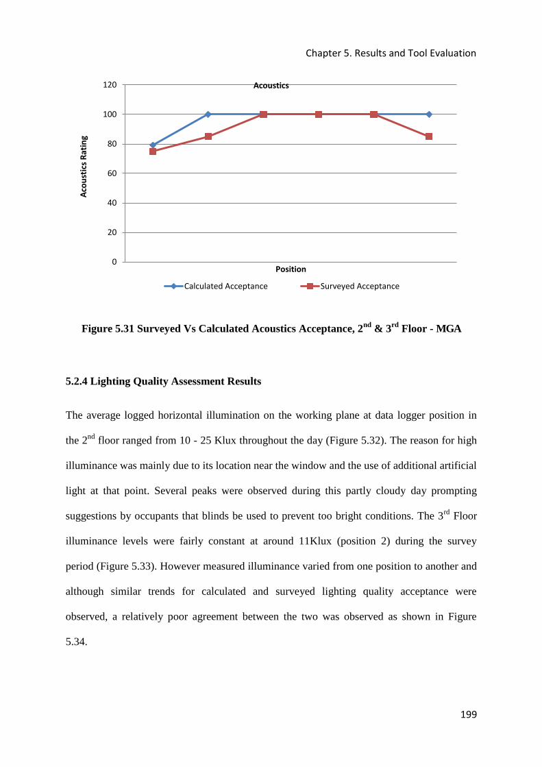
Chapter 5. Results and Tool Evaluation
199
Figure 5.31 Surveyed Vs Calculated Acoustics Acceptance, 2nd & 3rd Floor - MGA
5.2.4 Lighting Quality Assessment Results
The average logged horizontal illumination on the working plane at data logger position in
the 2nd floor ranged from 10 - 25 Klux throughout the day (Figure 5.32). The reason for high
illuminance was mainly due to its location near the window and the use of additional artificial
light at that point. Several peaks were observed during this partly cloudy day prompting
suggestions by occupants that blinds be used to prevent too bright conditions. The 3rd Floor
illuminance levels were fairly constant at around 11Klux (position 2) during the survey
period (Figure 5.33). However measured illuminance varied from one position to another and
although similar trends for calculated and surveyed lighting quality acceptance were
observed, a relatively poor agreement between the two was observed as shown in Figure
5.34.
0
20
40
60
80
100
120 A
cou
stic
s R
ati
ng
Position
Acoustics
Calculated Acceptance Surveyed Acceptance

Chapter 5. Results and Tool Evaluation
200
This could be explained by the use of less accurate spot measurement lux meters in some of
the positions and the rapid variation in illumination levels for offices that rely mostly on
daylighting during office hours. Overcrowding in the office also meant that some positions
were shielded from direct day lighting (for example, position 3 in the 2nd floor) and hence
they relied mostly on several 60W roof light bulbs hanging from the roof of the office. The
presence of additional table lamps also indicates that additional lighting is often required in
the office.
Figure 5.32 Logged Illuminance on a Working Plane Second Floor Office Space
(DT500) - MGA
Figure 5.33 Logged Illuminance on a Working Plane Third Floor Office Space (DT500)
– MGA

Chapter 5. Results and Tool Evaluation
201
Figure 5.34 Calculated vs. Surveyed Acceptance of Lighting in the offices - MGA
5.2.5 Indoor Environment Quality Assessment Results
The indoor environment in the Marsh Grochowski and Associates offices could be described
as a grade C office, consisting of crowded and lowly furniture levels, and less flexible
designs with poor finishes. The lobbies were poorly designed and decorated while the kitchen
and circulation areas were old fashioned although fairly well maintained. Some of the
features of the office are highlighted in Figures 5.35.
0
10
20
30
40
50
60
70
80
90
% s
ati
sfie
d/R
an
kin
g
Calculated lighting Acceptance Surveyed Lighting Acceptance

Chapter 5. Results and Tool Evaluation
202
Figure 5.35 Top Floor Office design, furniture levels, etc - MGA
IEQ values were calculated using the equation explained in Chapter 3 and the results showed
a standard deviation of 1.94 and a sample mean of 86.7. The minimum IEQ value was 83.6
and a maximum value of 89.6 was observed. This shows a fairly uniform calculated IEQ
throughout the office with most occupants thinking that the quality of the indoor environment
was acceptable.
However surveyed results showed large variations from one individual to another and this
could be attributed to the presence of individuals who suffer from conditions that affect their
perceptions of some aspects of the indoor environment. Measurements taken at their
workstations did not show much difference from the rest of the office. Calculated and
surveyed IEQ values were compared and using only results from healthy occupants they
showed fairly satisfactory agreements as shown in Figure 5.36. This is mainly due to the fact
that the adaptive thermal comfort index is applicable to a large group of people (de Dear,
2000) and only 4 valid responses were obtained from the office.

Chapter 5. Results and Tool Evaluation
203
Figure 5.36 Calculated Vs. Surveyed IEQ - MGA
Some occupants in their evaluation of IEQ expressed disappointment with the age of the
building, “the presence of single glazed windows and open triple height spaces” and
overcrowding.
5.2.6 Long Term Evaluation Capabilities of the IEQ Model
A second attempt at the applicability of the IEQ model for long term evaluation of the indoor
environment was tested in this case study for a period of two and half hours and the results
are summarised below. Measurements taken from position 2 first floor office between 11:30
AM and 2:00PM were used to test the model and the results are summarised in Table 5.9.
Results of thermal comfort, Acoustics, IAQ and IEQ are all shown in the table.
0
10
20
30
40
50
60
70
80
90
100
1 2 3 4
% S
ati
sfie
d/I
EQ
Ra
tin
g
Occupant
Model Predicted Surveyed
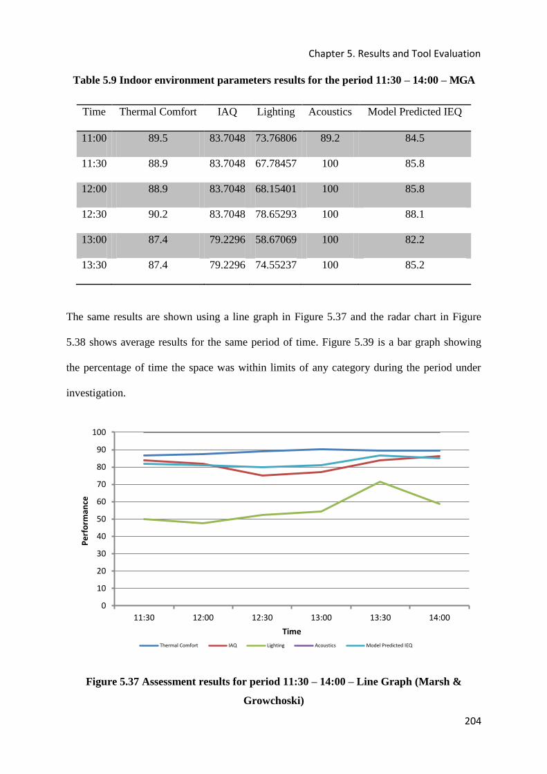
Chapter 5. Results and Tool Evaluation
204
Table 5.9 Indoor environment parameters results for the period 11:30 – 14:00 – MGA
Time Thermal Comfort IAQ Lighting Acoustics Model Predicted IEQ
11:00 89.5 83.7048 73.76806 89.2 84.5
11:30 88.9 83.7048 67.78457 100 85.8
12:00 88.9 83.7048 68.15401 100 85.8
12:30 90.2 83.7048 78.65293 100 88.1
13:00 87.4 79.2296 58.67069 100 82.2
13:30 87.4 79.2296 74.55237 100 85.2
The same results are shown using a line graph in Figure 5.37 and the radar chart in Figure
5.38 shows average results for the same period of time. Figure 5.39 is a bar graph showing
the percentage of time the space was within limits of any category during the period under
investigation.
Figure 5.37 Assessment results for period 11:30 – 14:00 – Line Graph (Marsh &
Growchoski)
0
10
20
30
40
50
60
70
80
90
100
11:30 12:00 12:30 13:00 13:30 14:00
Pe
rfo
rma
nce
Time
Thermal Comfort IAQ Lighting Acoustics Model Predicted IEQ

Chapter 5. Results and Tool Evaluation
205
Figure 5.38 Average assessment results for the period 11:30 – 14:00 - radar chart –
MGA
Figure 5.39 is shows that model calculated IEQ variables fell within the limits of specific
categories for 100% of the time therefore we can conclude that IEQ was category II, Thermal
comfort category III, Acoustics category I, Lighting category III and IAQ was category II.
Using area weighted averages IEQ was calculated for the office for the period 11:30 – 14:00
and the result is summarised in Table 5.10. The result (IEQ value) is the value that should be
compared to energy rating of the office for a specified period of time under investigation.
89
81
56
100
83
0
10
20
30
40
50
60
70
80
90
100
Thermal Comfort
IAQ
Lighting Acoustics
Model Predicted IEQ
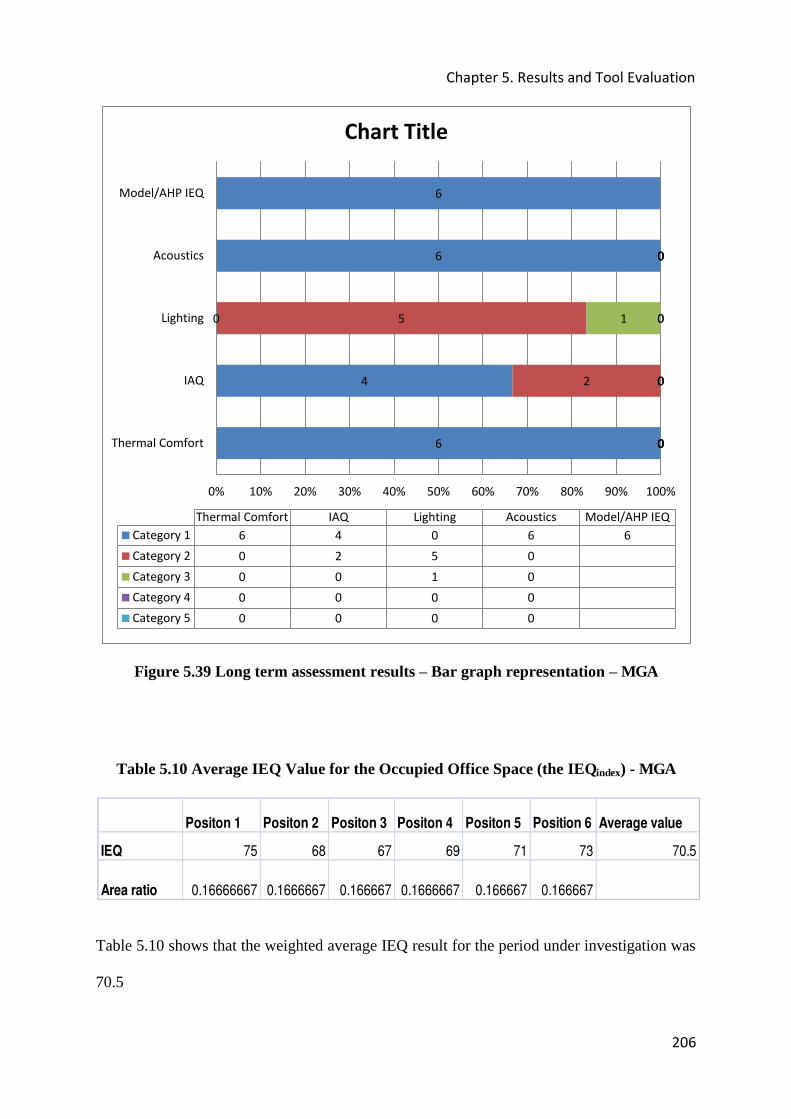
Chapter 5. Results and Tool Evaluation
206
Figure 5.39 Long term assessment results – Bar graph representation – MGA
Table 5.10 Average IEQ Value for the Occupied Office Space (the IEQindex) - MGA
Table 5.10 shows that the weighted average IEQ result for the period under investigation was
70.5
6
4
0
6
6
0
2
5
0
0
0
1
0
0
0
0
0
0
0
0
0
0% 10% 20% 30% 40% 50% 60% 70% 80% 90% 100%
Thermal Comfort
IAQ
Lighting
Acoustics
Model/AHP IEQ
Thermal Comfort IAQ Lighting Acoustics Model/AHP IEQ
Category 1 6 4 0 6 6
Category 2 0 2 5 0
Category 3 0 0 1 0
Category 4 0 0 0 0
Category 5 0 0 0 0
Chart Title
Positon 1 Positon 2 Positon 3 Positon 4 Positon 5 Position 6 Average value
IEQ 75 68 67 69 71 73 70.5
Area ratio 0.16666667 0.1666667 0.166667 0.1666667 0.166667 0.166667

Chapter 5. Results and Tool Evaluation
207
5.2.7 General Considerations for the Indoor Environment
Table 5.11 General checklist for the indoor environment – MGA
5.2.8 Conclusions and lessons learnt from the study
The study showed that naturally ventilated office buildings provide a greater challenge for
building owners to provide a consistently uniform indoor environment. The study showed
that occupants of naturally ventilated office tended to take individual action to improve
conditions in their work areas. Extra lamps, fans, portable electric heaters and selection of
clothing were evidence of the need to adjust to conditions in their workspaces. Decisions to
take “matters into their own hands” may prove very costly in terms of energy bills at the end
of the year as occupants use any method to keep themselves comfortable with little regards
for energy conservation.

Chapter 5. Results and Tool Evaluation
208
5.3 CASE STUDY 3: GRANBY HOUSE, NOTTINGHAM CITY CENTRE, UK
Case study 3 consists of offices situated on the first floor offices of Granby House on Friar
Lane in the centre of Nottingham City, United Kingdom. The office is a large open plan type
that has been split into several sections that include two general office spaces, a meeting
room, one cellular office space, a kitchenette, a store room, toilets and no reception area. This
property has been comprehensively refurbished including the common areas and the two
office suites. The open plan floor plates are rented by Hestia Managed Services on behalf of
the Energy Saving Trust and they are used as walk in advisory (and call centre) and
consultancy offices.
The office was occupied by white collar workers consisting of energy advisors, project
managers and consultants. Only the call centre area was studied and the occupants performed
sedentary activities such as typing, telephone conversations, filing, sorting of mail. Most
wore light office clothing consisting of trousers, shirt, tie and light shoes and in some cases
light office suites that included jackets. The level of furniture was medium with work stations
consisting of drawer desks, filing cabinets, printers and a medium size server placed openly
within the office space (bottom corner – marked S).
The HVAC system was mechanical with air supply grills located at the ceiling and a series of
radiators (unused) indicating the office was initially designed as a naturally ventilated one. A
small conventional gas boiler supplying hot water to the office was located in one of the
cabinets and almost all used in the office equipment was Grade A - energy efficient and
fitting the service provided by the business. A room thermostat was located in a centrally
located pillar and a remote control was available for adjusting temperature and air fan speed
as required by the occupants. The main features of the office building are summarised in the
Figure 5.40.
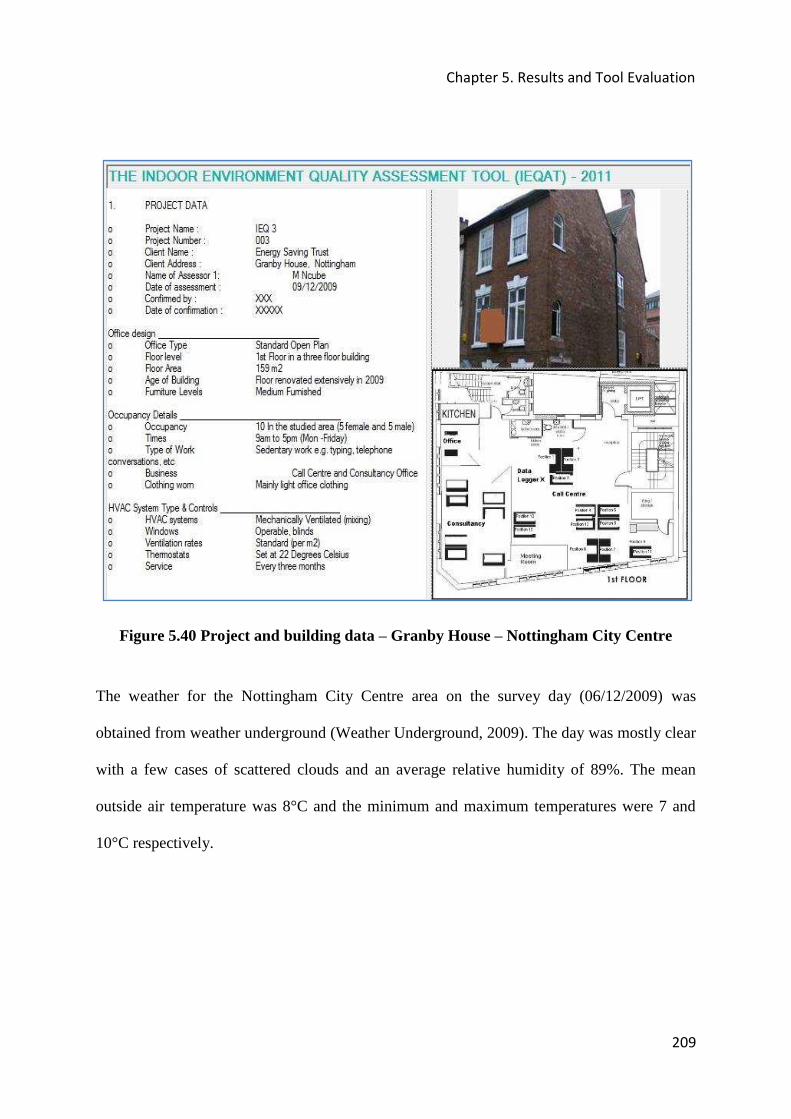
Chapter 5. Results and Tool Evaluation
209
Figure 5.40 Project and building data – Granby House – Nottingham City Centre
The weather for the Nottingham City Centre area on the survey day (06/12/2009) was
obtained from weather underground (Weather Underground, 2009). The day was mostly clear
with a few cases of scattered clouds and an average relative humidity of 89%. The mean
outside air temperature was 8°C and the minimum and maximum temperatures were 7 and
10°C respectively.

Chapter 5. Results and Tool Evaluation
210
5.3.1 Thermal Comfort, IAQ, Lighting and Acoustic Comfort Assessment Results
Following methodologies used in case studies 1 and 2, questionnaires were handed out to
occupants between 11:00 and 11:45AM during the survey day and measurement of variables
of interest was carried out before, during and after the questionnaire administration exercise.
Thermal comfort calculations were carried out using the VB program. The metabolic heat
production was estimated at 1.2 met and clothing levels were estimated at 1 clo based on
tables presented in Chapter 3. Model calculated PMV (all -0.1) values perfectly matched
surveyed ones (0) in an otherwise uniform thermal environment. IAQ, acoustic and lighting
comfort ratings were also computed using equations already described in Chapter 3 and the
results are summarised in Figure 5.42. The graphs show good agreement between model
calculated and survey results for IAQ, thermal comfort and acoustic comfort.
For lighting Model calculated results differed slightly from survey results for positions 8 – 10
while the rest of the positions showed very close agreement indicating that window locations
are generally associated with better satisfaction with the lighting environment. These
positions were closest to the windows and blinds were drawn during the survey period.
Figure 5.43 also shows that thermal comfort and IAQ were uniform throughout the office
floor suggesting that the mixing ventilation system was effective. Only one occupant
(position 10) expressed feelings of dry nose and they attributed this to the quality of indoor
air. As expected acoustic comfort rating fluctuated from one position to another since
background noise consisted mainly of abrupt, non continuous telephone conversations, filing,
drawers, telephones ringing and interpersonal conversations.
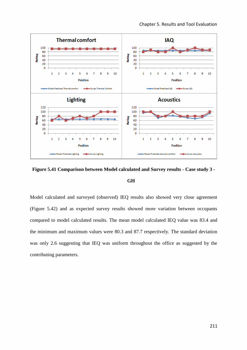
Chapter 5. Results and Tool Evaluation
211
Figure 5.41 Comparison between Model calculated and Survey results - Case study 3 -
GH
Model calculated and surveyed (observed) IEQ results also showed very close agreement
(Figure 5.42) and as expected survey results showed more variation between occupants
compared to model calculated results. The mean model calculated IEQ value was 83.4 and
the minimum and maximum values were 80.3 and 87.7 respectively. The standard deviation
was only 2.6 suggesting that IEQ was uniform throughout the office as suggested by the
contributing parameters.
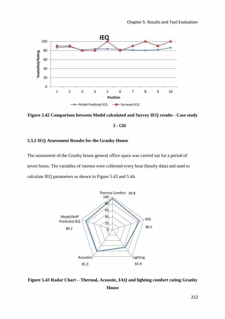
Chapter 5. Results and Tool Evaluation
212
Figure 5.42 Comparison between Model calculated and Survey IEQ results - Case study
3 - GH
5.3.2 IEQ Assessment Results for the Granby House
The assessment of the Granby house general office space was carried out for a period of
seven hours. The variables of interest were collected every hour (hourly data) and used to
calculate IEQ parameters as shown in Figure 5.43 and 5.44.
Figure 5.43 Radar Chart – Thermal, Acoustic, IAQ and lighting comfort rating Granby
House
0
20
40
60
80
100
1 2 3 4 5 6 7 8 9 10
%sa
tisf
ied
/Ra
tin
g
Position
IEQ
Model Predicted IEQ Surveyed IEQ
94.8
86.5
65.9 81.3
86.2 0
20
40
60
80
100 Thermal Comfort
IAQ
Lighting Acoustics
Model/AHP
Predicted IEQ
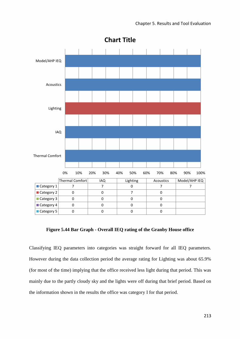
Chapter 5. Results and Tool Evaluation
213
Figure 5.44 Bar Graph - Overall IEQ rating of the Granby House office
Classifying IEQ parameters into categories was straight forward for all IEQ parameters.
However during the data collection period the average rating for Lighting was about 65.9%
(for most of the time) implying that the office received less light during that period. This was
mainly due to the partly cloudy sky and the lights were off during that brief period. Based on
the information shown in the results the office was category I for that period.
0% 10% 20% 30% 40% 50% 60% 70% 80% 90% 100%
Thermal Comfort
IAQ
Lighting
Acoustics
Model/AHP IEQ
Thermal Comfort IAQ Lighting Acoustics Model/AHP IEQ
Category 1 7 7 0 7 7
Category 2 0 0 7 0
Category 3 0 0 0 0
Category 4 0 0 0 0
Category 5 0 0 0 0
Chart Title

Chapter 5. Results and Tool Evaluation
214
5.3.3 General Checklist of the Granby House Office Space
A general checklist for the office was completed and the results showed that thermal comfort
data was readily available during the assessment unlike IAQ, acoustics and lighting which
either required more time or specialist knowledge and equipment to complete. The results of
the assessment are summarised in Table 5.12.
Table 5.12 General checklist for the indoor environment – Granby House
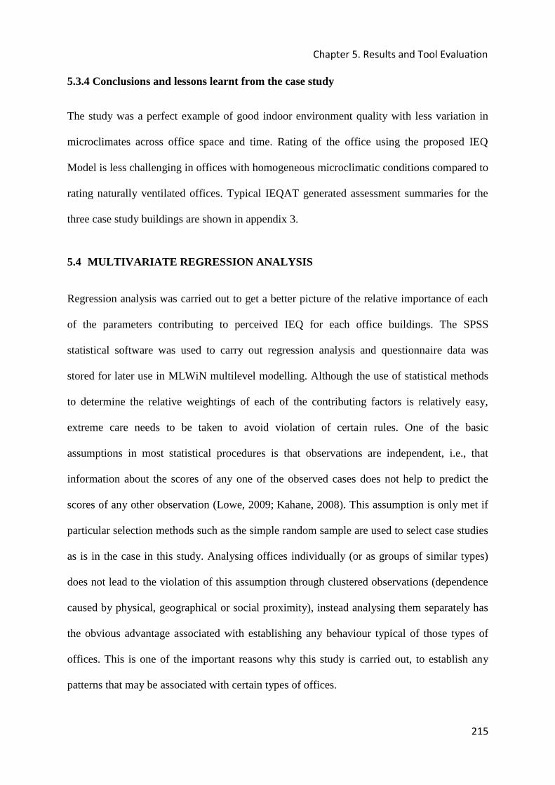
Chapter 5. Results and Tool Evaluation
215
5.3.4 Conclusions and lessons learnt from the case study
The study was a perfect example of good indoor environment quality with less variation in
microclimates across office space and time. Rating of the office using the proposed IEQ
Model is less challenging in offices with homogeneous microclimatic conditions compared to
rating naturally ventilated offices. Typical IEQAT generated assessment summaries for the
three case study buildings are shown in appendix 3.
5.4 MULTIVARIATE REGRESSION ANALYSIS
Regression analysis was carried out to get a better picture of the relative importance of each
of the parameters contributing to perceived IEQ for each office buildings. The SPSS
statistical software was used to carry out regression analysis and questionnaire data was
stored for later use in MLWiN multilevel modelling. Although the use of statistical methods
to determine the relative weightings of each of the contributing factors is relatively easy,
extreme care needs to be taken to avoid violation of certain rules. One of the basic
assumptions in most statistical procedures is that observations are independent, i.e., that
information about the scores of any one of the observed cases does not help to predict the
scores of any other observation (Lowe, 2009; Kahane, 2008). This assumption is only met if
particular selection methods such as the simple random sample are used to select case studies
as is in the case in this study. Analysing offices individually (or as groups of similar types)
does not lead to the violation of this assumption through clustered observations (dependence
caused by physical, geographical or social proximity), instead analysing them separately has
the obvious advantage associated with establishing any behaviour typical of those types of
offices. This is one of the important reasons why this study is carried out, to establish any
patterns that may be associated with certain types of offices.

Chapter 5. Results and Tool Evaluation
216
Regression analysis of the Leeds Town Centre House gives an adjusted R2 = 0.92 and a
significance F value of 1.86*e (-14) suggesting that the model has a lot to say about the
behaviour of the dependent variable. Thermal comfort (く = 0.23, p=0.35), IAQ (く = 0.35,
p=0.002), Acoustics (く = 0.13, p=0.43) and Lighting (く = 0.29, p=0.01). In this case we
reject the null hypothesis (Kahane, 2008) based on the significance value F. The constant has
been excluded from the regression analysis because firstly, and as expected, a case where all
independent variables are equal to zero must produce and IEQ rating of 0 (intercept on the x-
axis). Secondly regression results with a constant show a very poor association between the
contributors and IEQ (R2 = 0.42) and the model has a very poor p value for the constant
(0.82). The interpretation of the weightings for the Leeds Town Centre House is that, for
example, for a unit increase or decrease in thermal comfort the IEQindex increases or decreases
by 0.23 respectively, all else being equal. In terms of energy use any energy efficiency
measure that increases perceived thermal comfort by 1 unit will add 0.3 to the expected
perceived IEQ value. The same explanation applies to the coefficients derived below. The
results of this analysis are particular to this office and cannot therefore be generalised to other
naturally ventilated office buildings without the advantage of studying several similar offices
to establish pattern that may exist those types of offices.
Regression analysis of the MGA office showed that the resultant model explained the
behaviour of the dependent variable (adjusted R2 = 0.91). The model Significance, F is
4.07*e (-50) meaning that the model as a whole has a lot to say about perceived IEQ in that
office. Thermal comfort contributes the most to perceived IEQ with a く coefficient of 0.39
(p=0.02), followed by IAQ (く = 0.30, p=0.05), followed by lighting (く = 0.18, p=0.02) and
finally acoustics (く = 0.13, p=0.003).
Chapter 5. Results and Tool Evaluation
217
The Granby House regression produced adjusted R2 = 0.92, significance F = 1.6*e (-27), and
the weightings for contributors were thermal comfort (く = 0.28, p=0.06), IAQ (く = 0.32,
p=0.06), Acoustics (く = 0.23, p=0.085) and lighting (く = 0.16, p=0.008). The way
coefficients bounce about the weightings also varied from office to office with the highest
variance observed at the Leeds Town Centre House and the least at the Granby House.
Offices with IEQ conditions “typical” of natural, mechanical and mixed mode ventilation
need to be considered in order to get typical patterns for different office types. “Typical”
conditions are those conditions which are consistent with median values of data expected in
office buildings in the UK (BRECSU, 2000). Weightings need to be generated for all office
grades for both the heating and cooling seasons and recommendations for future research are
discussed in Chapter 6.
Table 5.13 compares regression coefficients derived from case studies and those from the
AHP. The Table suggests that different equations or models are required for different types of
offices and fitting questionnaire data to proposed models at occupant level (so called level 1)
does not necessarily produce resultant models that can be applicable to all offices. For
example the resultant weightings could work well for the Granby house and not for the
Marsh-Grochowski Associates and the Leeds Town Centre House. The coefficients also vary
from building to building for example the thermal comfort coefficient for the MGA office is
very high compared to the rest of the studies while the lighting coefficient for the Leeds
Town Centre House is higher than that of the other offices suggesting that different buildings
need to be accounted for using different models. It is also possible for variations to exist
between buildings of similar types and this can only be determined through extensive studies.
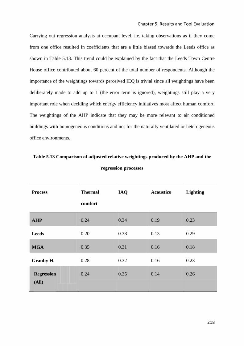
Chapter 5. Results and Tool Evaluation
218
Carrying out regression analysis at occupant level, i.e. taking observations as if they come
from one office resulted in coefficients that are a little biased towards the Leeds office as
shown in Table 5.13. This trend could be explained by the fact that the Leeds Town Centre
House office contributed about 60 percent of the total number of respondents. Although the
importance of the weightings towards perceived IEQ is trivial since all weightings have been
deliberately made to add up to 1 (the error term is ignored), weightings still play a very
important role when deciding which energy efficiency initiatives most affect human comfort.
The weightings of the AHP indicate that they may be more relevant to air conditioned
buildings with homogeneous conditions and not for the naturally ventilated or heterogeneous
office environments.
Table 5.13 Comparison of adjusted relative weightings produced by the AHP and the
regression processes
Process Thermal
comfort
IAQ Acoustics Lighting
AHP 0.24 0.34 0.19 0.23
Leeds 0.20 0.38 0.13 0.29
MGA 0.35 0.31 0.16 0.18
Granby H. 0.28 0.32 0.16 0.23
Regression
(All)
0.24 0.35 0.14 0.26
Chapter 5. Results and Tool Evaluation
219
5.5 Conclusions
Multivariate analysis shows that different types of offices environments need to be accounted
for using different models and that the AHP could be more suitable for air conditioned
homogeneous conditions. The exercise also shows that results cannot be generalised to all
office buildings in the UK since a very small number of offices have been used in this thesis.
More offices need to be investigated and any patterns that exist between different types of
offices need to be highlighted in the models. This highlights the importance of the multilevel
analysis approach to IEQ assessment which will be discussed further in the next chapter, and
which is a subject of future studies.

Chapter 6. Discussion of the Tool, Suggestions
for Future Work and Conclusions
220
6. Discussions, Suggestions for Future Work and Conclusions
6.1 GENERAL DISCUSSION AND SUGGESTED IMPROVEMENTS
The IEQAT is a promising novel tool that can be used for assessing the quality of the indoor
environment in office buildings in the UK. As explained earlier in Chapter 3 the IEQ model
was developed from proposed contributing factors using weighting of factors suggested by
Chiang and Lai (2002) AHP. The weightings were verified by fitting a regression model to
questionnaire results obtained from the occupants of three office buildings in the UK. It was
hoped that the relative weightings derived from regression would provide information which
would be more relevant to the UK situation since the case study buildings which were
selected for that purpose were located within that region.
The relative weightings shown in Table 5.11 suggest that AHP and regression model
(correlation) generated results are in close agreement for the Granby House and less so for
the other two buildings. As a universal index (taken at occupant level) the regression
generated model showed good correlation with observed IEQ results (Figure 5.47) with an R2
value of 0.94 and a significance (F) value of 3.91exp (-27). However looking at results at a
higher level (at office level) presents a different picture as offices that exhibited less
favourable indoor environment conditions agreed less with the AHP. This aspect needs to be
investigated further and more case studies need to be carried out to establish trends associated
with different IEQ conditions. Some researchers suggest that a number of subjective
observations greater than 500 are needed in order to minimise the errors in weightings
(Nemes et al, 2009).

Chapter 6. Discussion of the Tool, Suggestions
for Future Work and Conclusions
221
The IEQ index would be more powerful if cause and effect relationships could be established
between IEQ and contributing factors. Unfortunately the study was not been able to establish
important mechanisms of the relationships to be able to justify the study of the cause and
effect dimensions of this model. Studies have confirmed that it is difficult to isolate causes
from effects in buildings (Leaman and Bordass, 1999) and even if this was done an ideal IEQ
index would still require extensive knowledge on how human systems perceive IEQ and how
this relates to the risk of negative health outcome.
Perception of IEQ would be based on knowledge of how the human body reacts to stimuli
(IEQ variables) coming in via respective sensory organs (skin, ears, eyes, nose), how it
processes or screens the information and how the final perception of the indoor environment
is reached. This process needs to be explained physiologically; otherwise continued reliance
on predictive correlative studies will remain in place. The development of a thorough IEQ
model needs to take this study deeper into extensive experimentation involving human
subjects.
The accuracy of the IEQAT tool depends on the accuracy of the data used as input in the
calculations, for example the accuracy of measured data depends on the accuracy of the data
collection procedures and the equipment used. Similarly, the relative accuracy of simulation
data depends on the accuracy and quality of the simulation exercise. The accuracy of the
IEQAT also depends largely on the methodology used for its development. The assumptions
made in the development of assessment tools for thermal comfort, IAQ, acoustic comfort,
lighting and IEQ will influence the results and therefore influence the decision making
processes relating to energy use, comfort and even cost.
Chapter 6. Discussion of the Tool, Suggestions
for Future Work and Conclusions
222
6.1.1 Thermal Comfort Index
Thermal comfort calculation in air conditioned and mechanically ventilated office buildings
using ISO 7730 is the industry standard worldwide. The use of the PMV model to determine
perceived thermal comfort however has its limitations. Studies by Humphreys (Humphreys,
1994), noted that the PMV model was accurate (when compared with observed PMV) in
laboratory studies where occupants wore light clothing and carried out sedentary work but
was less accurate for heavier clothing and higher activity levels. Model calculated PMV
values were approximately 0.2 more than observed values in the Leeds Town Centre House,
and 0.1 less for the Granby House.
The Lace Market (Marsh Grochowski & Associates) building used the adaptive comfort
model and calculated % satisfaction results differed from observed ones by as much as 18%
and the reasons have already been explained in Chapter 5. Charles (Charles, 2003)
summarised studies by several researchers and concluded that the predicted and actual
thermal sensations differed for non neutral conditions and got larger the further away from
thermal neutrality one moved, and that occupants were more sensitive especially to changes
in temperature than the PMV model could predict under those conditions.
This conclusion was observed at the Leeds office where there was a slight difference between
predicted and observed PMV, and this could be due to the fact that questionnaires were
completed soon after sudden changes in temperature. Changes in temperature still had an
effect on the perceptions of thermal comfort for tens of minutes after the initial change was
recorded as indicated in the questionnaire responses. The results of the two mechanically
ventilated buildings show that PMVs are better estimated in uniform offices than in
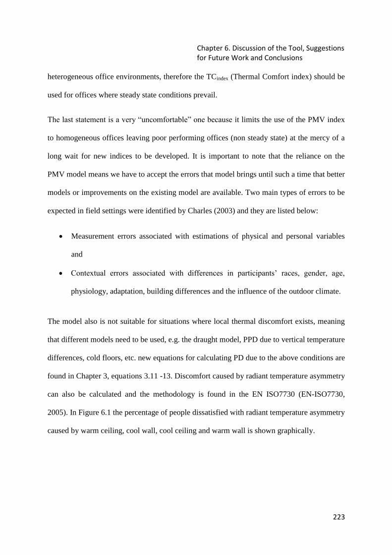
Chapter 6. Discussion of the Tool, Suggestions
for Future Work and Conclusions
223
heterogeneous office environments, therefore the TCindex (Thermal Comfort index) should be
used for offices where steady state conditions prevail.
The last statement is a very “uncomfortable” one because it limits the use of the PMV index
to homogeneous offices leaving poor performing offices (non steady state) at the mercy of a
long wait for new indices to be developed. It is important to note that the reliance on the
PMV model means we have to accept the errors that model brings until such a time that better
models or improvements on the existing model are available. Two main types of errors to be
expected in field settings were identified by Charles (2003) and they are listed below:
Measurement errors associated with estimations of physical and personal variables
and
Contextual errors associated with differences in participants’ races, gender, age,
physiology, adaptation, building differences and the influence of the outdoor climate.
The model also is not suitable for situations where local thermal discomfort exists, meaning
that different models need to be used, e.g. the draught model, PPD due to vertical temperature
differences, cold floors, etc. new equations for calculating PD due to the above conditions are
found in Chapter 3, equations 3.11 -13. Discomfort caused by radiant temperature asymmetry
can also be calculated and the methodology is found in the EN ISO7730 (EN-ISO7730,
2005). In Figure 6.1 the percentage of people dissatisfied with radiant temperature asymmetry
caused by warm ceiling, cool wall, cool ceiling and warm wall is shown graphically.
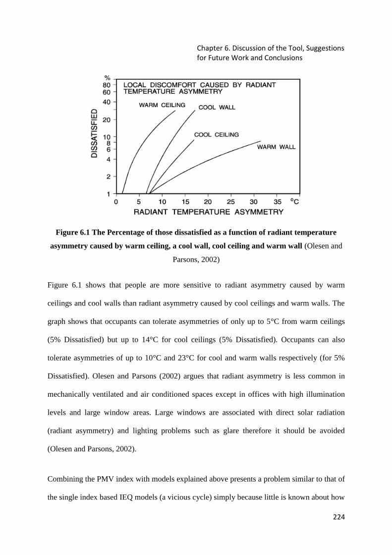
Chapter 6. Discussion of the Tool, Suggestions
for Future Work and Conclusions
224
Figure 6.1 The Percentage of those dissatisfied as a function of radiant temperature
asymmetry caused by warm ceiling, a cool wall, cool ceiling and warm wall (Olesen and
Parsons, 2002)
Figure 6.1 shows that people are more sensitive to radiant asymmetry caused by warm
ceilings and cool walls than radiant asymmetry caused by cool ceilings and warm walls. The
graph shows that occupants can tolerate asymmetries of only up to 5°C from warm ceilings
(5% Dissatisfied) but up to 14°C for cool ceilings (5% Dissatisfied). Occupants can also
tolerate asymmetries of up to 10°C and 23°C for cool and warm walls respectively (for 5%
Dissatisfied). Olesen and Parsons (2002) argues that radiant asymmetry is less common in
mechanically ventilated and air conditioned spaces except in offices with high illumination
levels and large window areas. Large windows are associated with direct solar radiation
(radiant asymmetry) and lighting problems such as glare therefore it should be avoided
(Olesen and Parsons, 2002).
Combining the PMV index with models explained above presents a problem similar to that of
the single index based IEQ models (a vicious cycle) simply because little is known about how

Chapter 6. Discussion of the Tool, Suggestions
for Future Work and Conclusions
225
the indices can be added to produce one representative value and that PPD values overlap i.e.
those dissatisfied with draughts could also be dissatisfied with temperature, and so on. The
equations discussed above need to be added to the IEQAT to improve its performance.
Naturally ventilated offices use different criteria for thermal comfort as explained in Chapters
2, 3 and 5.
The effects of physical variables affecting thermal comfort on perceived IEQ is important for
purposes of establishing the link between energy use and occupant comfort. It is essential for
example, to get an idea of how much influence a change in temperature can bring to
perceived IEQ for purposes of programming the tool. To investigate the effects of each of the
variables at all possible conditions (various office microclimates) would require too many
equations and this would be time consuming and nearly impossible to complete. However the
problem could be easily solved using a computer program (Computer Code) therefore the
formulations could be included in the IEQAT’s modelling capabilities. Example Equations
linking variables to IEQ are derived in the next paragraphs.
The Effects of Air and Mean Radiant Temperature on Thermal Comfort
Figure 6.2 shows the relationship between Thermal comfort rating and, air and mean radiant
temperature. By showing the effects of temperatures on thermal comfort we can demonstrate
their impact on occupant comfort since thermal comfort forms part of IEQ acceptance. The
turning point of the curve is the set point (neutrality temperature). The graphs were produced
by varying air and mean radiant temperature and keeping all other variables constant. For
offices where mean radiant temperature differs from air temperature individual equations can
be produced and added into the computer code to cater for the effects of each of the
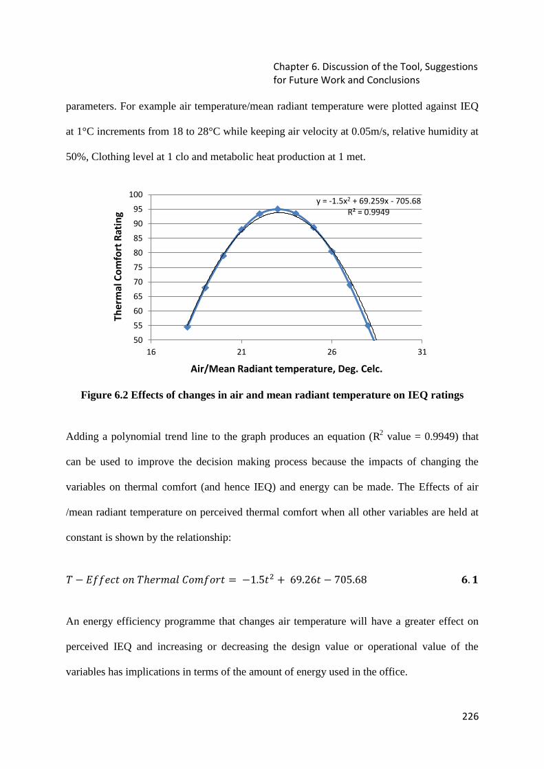
Chapter 6. Discussion of the Tool, Suggestions
for Future Work and Conclusions
226
parameters. For example air temperature/mean radiant temperature were plotted against IEQ
at 1°C increments from 18 to 28°C while keeping air velocity at 0.05m/s, relative humidity at
50%, Clothing level at 1 clo and metabolic heat production at 1 met.
Figure 6.2 Effects of changes in air and mean radiant temperature on IEQ ratings
Adding a polynomial trend line to the graph produces an equation (R2 value = 0.9949) that
can be used to improve the decision making process because the impacts of changing the
variables on thermal comfort (and hence IEQ) and energy can be made. The Effects of air
/mean radiant temperature on perceived thermal comfort when all other variables are held at
constant is shown by the relationship:
劇 伐 継血血結潔建 剣券 劇月結堅兼欠健 系剣兼血剣堅建 噺 伐な┻の建態 髪 はひ┻には建 伐 ばどの┻はぱ 掃┻ 層
An energy efficiency programme that changes air temperature will have a greater effect on
perceived IEQ and increasing or decreasing the design value or operational value of the
variables has implications in terms of the amount of energy used in the office.
y = -1.5x2 + 69.259x - 705.68
R² = 0.9949
50
55
60
65
70
75
80
85
90
95
100
16 21 26 31
Th
erm
al
Co
mfo
rt R
ati
ng
Air/Mean Radiant temperature, Deg. Celc.

Chapter 6. Discussion of the Tool, Suggestions
for Future Work and Conclusions
227
The Effects of Air Velocity on Thermal comfort
The effects of air velocity (including its temperature dependence) on perceived thermal
comfort is illustrated in Figure 6.3. Plots of varying ち (above and below a temperature set
point, e.g. 23°C) against thermal comfort rating at various temperatures are illustrated. For
example at 22°C increasing air velocity has a negative effect on thermal comfort whereas at
26°C it has a positive effect. The relationships between air velocity and thermal comfort at
22°C and 26°C are shown by equations 6.2 and 6.3 respectively.
劇潔 堅欠建件券訣 噺 ひの┻ばぱ 茅 結貸待┻戴腿胎掴 掃┻ 匝
劇系 堅欠建件券訣 噺 ね┻ぱひば 岫懸岻 髪 ひね┻ばに 掃┻ 惣
Increasing air velocity means more energy is used to pump the air at higher flow rates and the
effects on thermal comfort and IEQ need to be programmed accurately if comparisons are to
be made.
Figure 6.3 Effects of Air Velocity on Thermal Comfort
y = 95.775e-0.387x
y = 4.8966ln(x) + 94.719
75
80
85
90
95
100
0.05 0.1 0.15 0.2 0.25 0.3 0.35 0.4
Th
erm
al
Co
mfo
rt r
ati
ng
Air velocity (m/s)
TC (22) TC (23) TC (25) TC (26) Expon. (TC (22)) Log. (TC (26))

Chapter 6. Discussion of the Tool, Suggestions
for Future Work and Conclusions
228
The Effects of Relative Humidity on IEQ
A plot of relative humidity against IEQ is shown in Figure 6.4 and the graph shows that the
effects of relative humidity are highest nearer to RH value of 50%. The trend line produced in
the graph has an R2 value of 0.95 suggesting a strong association between the two variables of
equation 6.4.
Figure 6.4 Effects of Relative Humidity on IEQ
Humidification and dehumidification processes are energy intensive hence the effects of
changing humidity levels in supply air on perceived IEQ need to be known to office
designers. The Effects of Relative Humidity on perceived IEQ when all other variables are
constant is shown by the relationship:
荊継芸 堅欠建件券訣 噺 伐ど┻どどどね岫迎茎岻態 髪 ど┻どどぬぱば岫迎茎岻 髪 ばは┻のねな 掃┻ 想
76.4
76.6
76.8
77
77.2
77.4
77.6
0 20 40 60 80 100
IEQ
Ra
tin
g
RH (%)
Effects of RH on IEQ

Chapter 6. Discussion of the Tool, Suggestions
for Future Work and Conclusions
229
6.1.2 The IAQ Index
The IAQ assessment model presented in this thesis only uses three forms of input namely
CO2 concentration, air pollution level in decipol and ventilation rates to calculate perceived
IEQ. In this thesis only the CO2 route was investigated leaving the other two open to further
investigation although these methods are generally accepted as correlating well with
perceived IAQ. The results of IAQ assessment of office buildings showed a good agreement,
as explained in Chapter 5, with observed values bouncing about the model calculated ones in
the Leeds Town Centre House study, and the model overestimating perceived IAQ in the
Lace Market office study. The model was almost perfect for the Granby House - again
indicating (as in thermal comfort assessment) that IEQ models tend to do better in air
conditioned homogeneous environments. The model’s performance depends on the quality of
input data hence data collection methods and equipment needs to be of the required standard
in order to reduce the size of error in calculation.
A comprehensive approach to IAQ assessment has been urged on by researchers
(Moschandreas and Sofuoglu, 2003) although there is still a long way before an index that
takes into account all parameters relevant to IAQ assessment is developed. An ideal model,
which at present is beyond the realms of a PhD study, should include a database of all known
factors that cause dissatisfaction with the quality of indoor air including all factors known to
cause negative health effects. This should include the sources of pollution, source strengths
and the kinetics of release of pollutants. Exposure – effect relationships for all pollutants
listed in the database needs to be documented and a formula or model that shows the additive
or combined effects of combinations of pollutants needs to be developed. Kinetics should
express both health and comfort (satisfaction) effects of relative quantities of known

Chapter 6. Discussion of the Tool, Suggestions
for Future Work and Conclusions
230
pollutants. Equation 6.4 shows a hypothetical IAQ expressed as a function of known
pollutants (summation of pollutant concentrations multiplied by their relative weightings).
荊畦芸 蛤 蕃布鶏沈激沈津沈退怠 否 掃┻ 捜
Unfortunately such expressions would take a long time to develop hence for the time being
calculations will have to depend on information available in literature, whilst urging research
forward.
A graph that shows the relationship between IAQ and IEQ is shown in Figure 6.5 and an
equation showing the same relationship is shown by equation 6.6. The equation can be used
to make choices on which variables to manipulate in order to improve energy efficiency in
the office. For example, Changing CO2 concentrations could involve increasing ventilation
rates, a decision that could increase electrical power consumed by the pumps and fans.
Figure 6.5 Effects of Indoor CO2 Concentrations on IEQ
70
71
72
73
74
75
76
77
78
0 200 400 600 800 1000 1200
IEQ
ra
tin
g
CO2 concentration above Oudoor
Effects of CO2 conc above Outdoor on IEQ
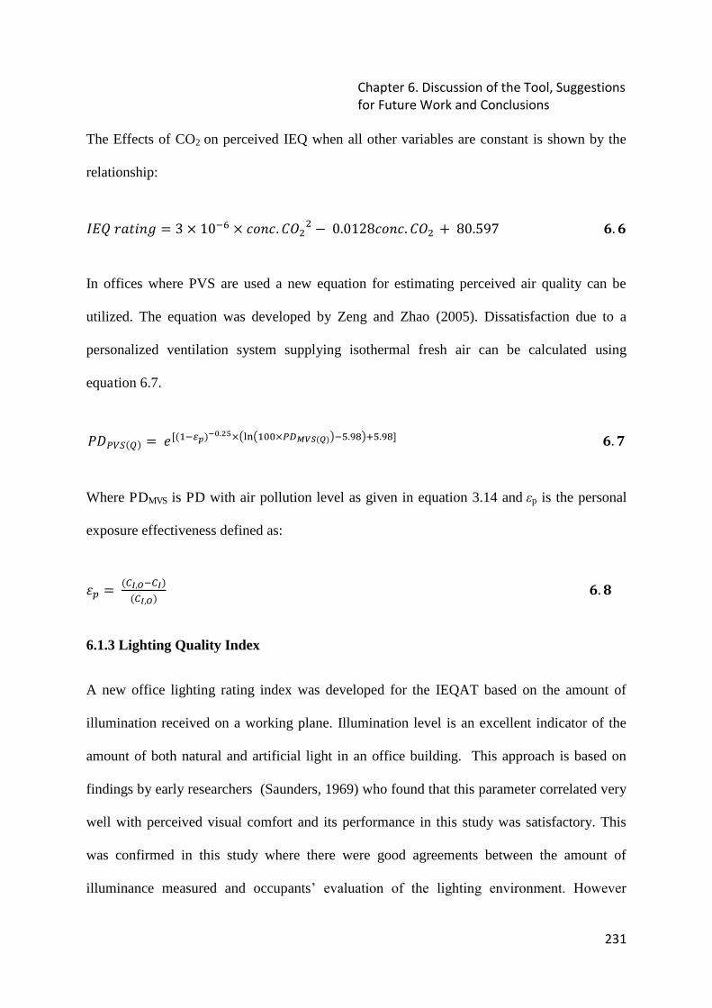
Chapter 6. Discussion of the Tool, Suggestions
for Future Work and Conclusions
231
The Effects of CO2 on perceived IEQ when all other variables are constant is shown by the
relationship:
荊継芸 堅欠建件券訣 噺 ぬ 抜 など貸滞 抜 潔剣券潔┻ 系頚態態 伐 ど┻どなにぱ潔剣券潔┻ 系頚態 髪 ぱど┻のひば 掃┻ 掃
In offices where PVS are used a new equation for estimating perceived air quality can be
utilized. The equation was developed by Zeng and Zhao (2005). Dissatisfaction due to a
personalized ventilation system supplying isothermal fresh air can be calculated using
equation 6.7.
鶏経牒蝶聴岫町岻 噺 結岷岫怠貸悌妊岻貼轍┻鉄天抜盤狸樽盤怠待待抜牒帖謎楠縄岫楢岻匪貸泰┻苔腿匪袋泰┻苔腿峅 掃┻ 挿
Where PDMVS is PD with air pollution level as given in equation 3.14 and ip is the personal
exposure effectiveness defined as:
綱椎 噺 岫寵内┸捺貸寵内岻岫寵内┸捺岻 掃┻ 掻
6.1.3 Lighting Quality Index
A new office lighting rating index was developed for the IEQAT based on the amount of
illumination received on a working plane. Illumination level is an excellent indicator of the
amount of both natural and artificial light in an office building. This approach is based on
findings by early researchers (Saunders, 1969) who found that this parameter correlated very
well with perceived visual comfort and its performance in this study was satisfactory. This
was confirmed in this study where there were good agreements between the amount of
illuminance measured and occupants’ evaluation of the lighting environment. However
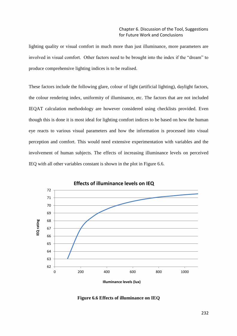
Chapter 6. Discussion of the Tool, Suggestions
for Future Work and Conclusions
232
lighting quality or visual comfort in much more than just illuminance, more parameters are
involved in visual comfort. Other factors need to be brought into the index if the “dream” to
produce comprehensive lighting indices is to be realised.
These factors include the following glare, colour of light (artificial lighting), daylight factors,
the colour rendering index, uniformity of illuminance, etc. The factors that are not included
IEQAT calculation methodology are however considered using checklists provided. Even
though this is done it is most ideal for lighting comfort indices to be based on how the human
eye reacts to various visual parameters and how the information is processed into visual
perception and comfort. This would need extensive experimentation with variables and the
involvement of human subjects. The effects of increasing illuminance levels on perceived
IEQ with all other variables constant is shown in the plot in Figure 6.6.
Figure 6.6 Effects of illuminance on IEQ
62
63
64
65
66
67
68
69
70
71
72
0 200 400 600 800 1000
IEQ
ra
tin
g
Illuminance levels (lux)
Effects of illuminance levels on IEQ
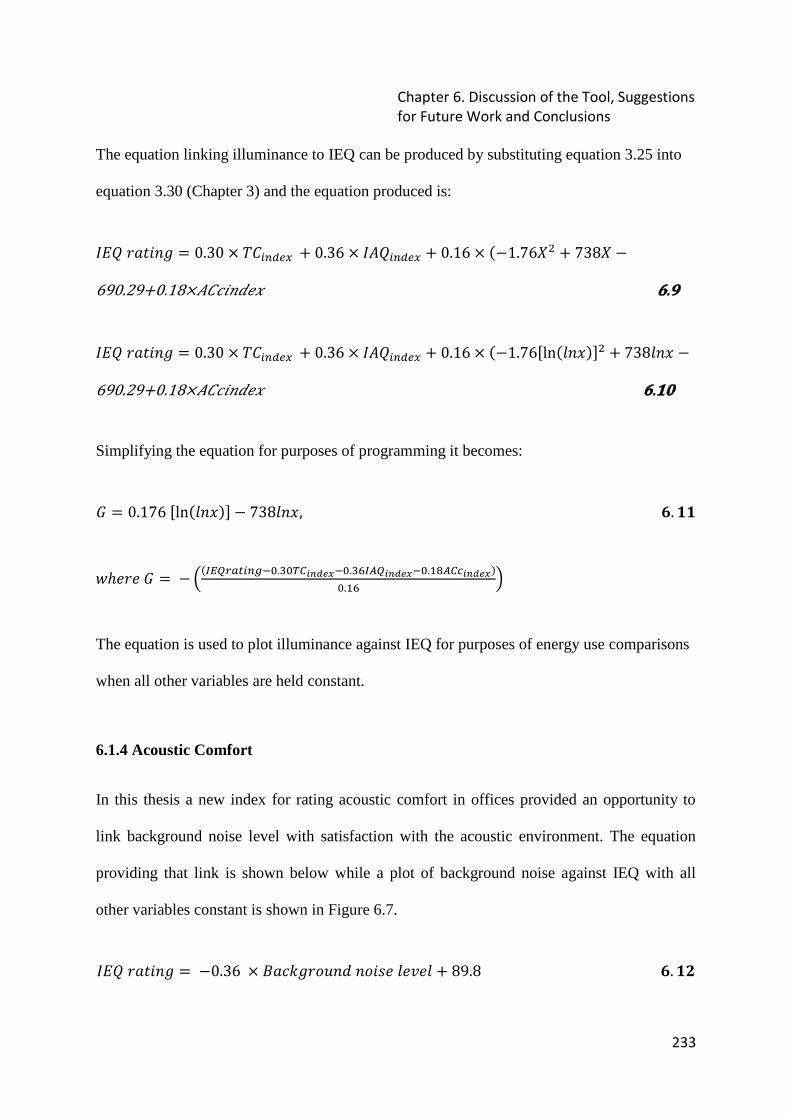
Chapter 6. Discussion of the Tool, Suggestions
for Future Work and Conclusions
233
The equation linking illuminance to IEQ can be produced by substituting equation 3.25 into
equation 3.30 (Chapter 3) and the equation produced is:
荊継芸 堅欠建件券訣 噺 ど┻ぬど 抜 劇系沈津鳥勅掴 髪 ど┻ぬは 抜 荊畦芸沈津鳥勅掴 髪 ど┻なは 抜 岫伐な┻ばは隙態 髪 ばぬぱ隙 伐690.29+0.18×畦系潔件券穴結捲 掃.操
荊継芸 堅欠建件券訣 噺 ど┻ぬど 抜 劇系沈津鳥勅掴 髪 ど┻ぬは 抜 荊畦芸沈津鳥勅掴 髪 ど┻なは 抜 岫伐な┻ばは岷 岫健券捲岻峅態 髪 ばぬぱ健券捲 伐690.29+0.18×畦系潔件券穴結捲 掃.層宋
Simplifying the equation for purposes of programming it becomes:
罫 噺 ど┻なばは 岷 岫健券捲岻峅 伐 ばぬぱ健券捲┸ 掃┻ 層層
拳月結堅結 罫 噺 伐 岾岫彫帳町追銚痛沈津直貸待┻戴待脹寵日韮匂賑猫貸待┻戴滞彫凋町日韮匂賑猫貸待┻怠腿凋寵頂日韮匂賑猫岻待┻怠滞 峇 The equation is used to plot illuminance against IEQ for purposes of energy use comparisons
when all other variables are held constant.
6.1.4 Acoustic Comfort
In this thesis a new index for rating acoustic comfort in offices provided an opportunity to
link background noise level with satisfaction with the acoustic environment. The equation
providing that link is shown below while a plot of background noise against IEQ with all
other variables constant is shown in Figure 6.7.
荊継芸 堅欠建件券訣 噺 伐ど┻ぬは 抜 稽欠潔倦訣堅剣憲券穴 券剣件嫌結 健結懸結健 髪 ぱひ┻ぱ 掃┻ 層匝

Chapter 6. Discussion of the Tool, Suggestions
for Future Work and Conclusions
234
Figure 6.7 Effects of Background noise level on IEQ
The index performed very well for all case studies despite complications associated with
sudden fluctuations in sound pressure levels caused by abrupt speech and the untimely
ringing of the telephone, etc. The Lace market office (naturally ventilated office) showed
more variation in observed acoustic comfort ratings than the Town Centre House and the
Granby House.
This could be due to the location of the office and its poor sound proofing walls and windows
that allowed noise from outside to be heard by the occupants. However the acoustic comfort
index still needs to be improved so that it takes into account all other factors that may be
relevant to occupant’s perception of the acoustic environment. Important factors such as
sound frequency, power, etc need to be weighted in when considering future acoustic comfort
indices.
55
60
65
70
75
80
85
15 25 35 45 55 65 75 85 95
IEQ
Ra
tin
g
Background Noise Level (dBA)
Effects of Background Noise Level on IEQ
Chapter 6. Discussion of the Tool, Suggestions
for Future Work and Conclusions
235
6.1.5 Important features of the IEQAT
The IEQAT methodology developed in this thesis allows the calculation of thermal comfort,
IAQ, acoustic, lighting comfort and perceived IEQ using the same variables used for building
energy performance evaluation. This approach allows comparisons to be made between the
two aspects of building performance and encourages decisions that provide the best balance
between occupant comfort and energy use. This tool is designed to be used for assessment of
all types of offices and similar buildings in the UK using the following types of data as input:
Design;
Calculated;
Measured; and
Questionnaire (survey) data.
The results of the assessments (quantities) can be calculated on any one of the following basis
depending on the amount of data that has been collected:
Instantaneous (real time);
Hourly;
Daily;
Weekly;
Monthly;
Seasonal; and
Annual.

Chapter 6. Discussion of the Tool, Suggestions
for Future Work and Conclusions
236
Using this tool it is possible to compute IEQ and other results for any part of an office
building space i.e. assessments can be carried out for the following:
Whole buildings; and
Parts of buildings.
Tenants within the same building could chose to have different IEQ assessment certificates /
ratings based on the performance of the tenanted area. This is particularly important in
buildings that have a degree of variation in microclimates due to factors such as tenant
location, poor design of the HVAC systems, etc. The tool also makes it possible to assess
buildings at any stage of construction, i.e. from design stages right up to post occupancy
evaluation stages hence it has potential to be used as a design tool that sets sustainable design
priorities for engineers and determines which energy efficiency measures provide a good
balance between environmental performance and occupant comfort. It can also be used as a
management tool to organise and control variables that affect energy use and cost without
sacrificing human comfort and productivity. It helps with identifying problem areas that
should be given priority when considering improving the quality of the Indoor environment.
The office rating system is also important for the following reasons:
it provides market recognition for high performing buildings
it can be used to negotiate tenancies
it gives a competitive advantage to better quality offices
encourages best practice in commercial buildings

Chapter 6. Discussion of the Tool, Suggestions
for Future Work and Conclusions
237
The IEQAT therefore can either be used for voluntary assessment of office spaces or
enforced in the form of legislation should the need arise. It can be used to improve current
assessment tools by incorporating it into comprehensive Building Environment Performance
tools.
6.2 GENERAL CONCLUSIONS
This thesis demonstrates the need to develop IEQ assessment methodologies that can be used
in office buildings in the UK and worldwide. The European directive on the energy
performance of buildings has challenged researchers to develop energy assessment tools and
these have been developed successfully. Some of the tools are currently being used to
produce energy performance certificates for domestic and commercial buildings. Most of
these tools have calculated energy performance based on criteria used for the indoor
environment. However a declaration of energy use without declarations of IEQ does not
make sense simply because it is possible to design energy efficient buildings that are
uninhabitable.
Energy performance certificates do not provide much information, if any, on the quality of
the indoor environment hence the need to develop this tool. Current buildings assessment
tools are biased towards comprehensive assessment of the environment performance of
buildings and with less focus on building IEQ assessment tools that reflect the occupant’s
perception of the indoor environment.

Chapter 6. Discussion of the Tool, Suggestions
for Future Work and Conclusions
238
6.2.1 IEQ Indices
Early indices on thermal comfort, IAQ, Acoustics and lighting were derived from literature
review. Thermal comfort assessment indices proved to be the most developed of the four
indices and hence the ISO 7730 thermal comfort assessment standard which is based on the
PMV model was adopted. PMV and PPD indices allow office spaces to be rated according to
the ratio of people dissatisfied with the thermal environment.
This approach provided a foundation on which other indices were developed in this study.
Studies on the performance of the PMV model have been carried out on different types of
buildings across the globe and recommendations have been put forward to the wider public.
A computer program based on based on Fanger’s thermal comfort model was developed quite
easily using the VB program and the full program code is found in the Appendix.
IAQ indices proved more difficult to produce mainly due to the large (hundreds) numbers and
the complex nature of parameters contributing to IAQ acceptance. The parameters include
particulates, gases, organic compounds, chemicals, and biological agents which are very
difficult to quantify in indoor air. Their effects on health and well being of occupants depend
on the complex kinetics that are not well understood and need several years of further
investigation. A few assessment methods suggested in literature included those based on the
IAQ guidelines hence ventilation rates, CO2 concentrations and air pollution levels in decipol
were adopted for this index.
Acoustic comfort indices which reflected satisfaction with the indoor environment could not
be established from literature. Most noise rating techniques were useful for design and
dimensioning of office buildings but they neither reflected satisfaction with the acoustic
Chapter 6. Discussion of the Tool, Suggestions
for Future Work and Conclusions
239
environment nor reflected on correlation to productivity. A new acoustic comfort index was
developed based on the results of research studies that compared noise levels with
satisfaction with the indoor noise levels. The lack of information on assessment approaches
that reflect or correlate with human evaluation echoed problems that were encountered with
all other indices.
Lighting indices were no exception. Lighting guides have been produced by regulatory
bodies and standards associations and a few reflect occupant satisfaction, or lack of, with
their internal environment. In this thesis a lighting quality index based on the findings of
research carried out by Saunders (Saunders, 1969) was developed and this finally paved way
for the development of the IEQ index. The IEQ assessment methodology is based on the IEQ
model, a linear relationship between IEQ and contributing parameters explained above. The
relative weightings of each of the contributors were obtained from AHP studies carried out by
Chiang et al (Chiang and Lai, 2002) and the weightings were verified using the study of
three selected case study buildings.
6.2.2 The Case study Buildings
Case study buildings were selected from a list of office buildings in the UK. Offices which
were different from each other in a variety of ways were selected in order to allow for better
generalisation of results. These included a naturally ventilated - pre war office building
situated in an urban location, a mixed mode - post 1996 refurbished - urban office building
and a modern mechanically ventilated office building located in a city centre.
Chapter 6. Discussion of the Tool, Suggestions
for Future Work and Conclusions
240
The case study buildings were used largely for two purposes:
To verify the IEQ model developed in Chapter 3 and
To derive relative weightings of each of the contributing factors.
Model based IEQ assessments were carried out using data collected from the case study
buildings as input. Measurement of variables necessary for the calculation of IEQ was carried
out using specialised equipment which included a data logger and several sensors. Extreme
care was exercised in the selection of the equipment and therefore only high precision and
relevant equipment was used. In order to verify the performance of the model its results were
compared to the results of subjective assessment of the indoor environment.
Subjective assessment results were also required for purposes of deriving coefficients
therefore a study design was developed. Questionnaires were used to collect subjective
evaluations of the offices and they were administered at a time when measurements were
taken in order to get a better understanding of the patterns that prevailed within the buildings.
It was concluded that the weightings (coefficients) compared well with those from the AHP
and that regression coefficients were better suited to the UK situation since case study
buildings were all within the UK.
Model calculated results compared well with subjective evaluations hence it was concluded
that the IEQAT methodology was appropriate for rapid assessment of IEQ in office buildings
in the UK. However in order to generate weightings that can be generalised to all office
buildings in the UK a study that is longer than a normal PhD period may be required.

Chapter 6. Discussion of the Tool, Suggestions
for Future Work and Conclusions
241
6.2.3 The IEQ Model
The conclusions on the final IEQ model developed in this work include the following:
The development a model that reflects the opinion of the occupant;
The use of variables that are used in the calculation of building energy performance
for the calculation of IEQ;
The potential of the IEQAT to be used as a design, management and compliance tool;
The potential of the tool to be incorporated into the BMS and into comprehensive
building environmental assessment tools; and
The development of a tool which is more applicable to air conditioned office
buildings with uniform conditions.
6.3 RECOMMENDATIONS FOR FUTURE RESEARCH
The work produced in this study represents the first attempt at using weightings derived from
subjective evaluation of indoor environments to develop a methodology for assessment of
IEQ in occupied office spaces in the UK. It needs to be followed up by rigorous evaluation of
the IEQ Model by studying a number of selected office building and in some cases
continuously for a period of more than a year. During this time questionnaires need to be
administered to capture occupants’ long term evaluation of the indoor environment and
standard questionnaires such as the BUS occupant surveys could be administered periodically
in conjunction with the IEQ assessment questionnaire presented in this thesis (Appendix 2)
for verification purposes where possible.

Chapter 6. Discussion of the Tool, Suggestions
for Future Work and Conclusions
242
The exercise allows the following types of data to be captured for comparative analysis:
Design data (as designed),
Measured data some of which may be captured via the BMS and through the use of a
data logger connected to remote sensors that are located strategically across the office
space.
Modelling data which can be obtained from extensive simulation of the indoor
environment using validated models. Examples of variables collected this way may
include lighting data, thermal comfort variables, selected IAQ data such as pollutant
distribution over time (CFD analysis), and sound pressure level estimation using
relevant equations (Rasmussen, 1999). Simulations should include energy
performance analyses using approved software such as the Bentley HEVACOMP
software (described in Chapter 3).
In order to improve on the accuracy of relative weightings of the parameters contributing to
IEQ multi level analysis needs to be carried out to investigate the effects of clustering at other
(or higher) levels of investigation. For example the relative weightings may vary depending
on age or gender of occupants, geographic location of office, type of office building, or social
class of the occupants.
More studies need to be carried out in order to establish the trends across different types of
environments and groups. Continued study of different types of office buildings could also
lead to the establishment of benchmarks for performance and the setting of minimum
standards below which office buildings are considered to have failed the IEQ test. Multi level
analysis can be complex and time consuming and a more viable alternative would be to carry

Chapter 6. Discussion of the Tool, Suggestions
for Future Work and Conclusions
243
out physiological studies on office occupants. Such studies could include climate chamber
studies where occupants are subjected to varying stimuli (pure experiments) and their
subjective assessment of the microclimates are captured using questionnaires. Physiology
based studies would strongly back predictive models.
Finally a computer program based on the IEQ model needs to be developed. The tool needs
to incorporate an energy performance assessment methodology so that both IEQ and energy
performance analysis can be carried out at once and results can be compared (using dynamic
simulation capabilities of the tool). A cost analysis section that gives a third dimension to the
tool could also be a welcome addition. Costs of energy saving or comfort enhancement
actions could help decide whether these initiatives are economically viable or not. For
example replacing an incandescent bulb with a fluorescent one may be productive in terms of
lighting comfort and energy saving but it could cost more. Economic appraisal of energy
systems adds a good dimension to the tool.
A database of building construction materials, their polluting power and sound propagation
characteristics, weather data, lighting ensembles, air pollution levels, typical outside air CO2
levels in the UK could be added to the tool. The addition of CAD capabilities into the tool
allows the construction of model buildings by specifying materials and plans hence energy
and IEQ analyses could be carried out from the same project.
References
244
7. References
Acoustics, <http://www.acoustics.com/> Access date: 01/07/2009.
Adnot, J., 2003, Energy Efficiency and Certification of Central Air Conditioners (EECCAC) D. G., Transportation-Energy (DGTREN) of the Commission of the E. U.
Ameen, A., 2006, Refrigeration and Air Conditioning, New Delhi, Prentice-Hall of India.
ASHRAE, 1984, ASHRAE Guide - Fundamentals, American Society of Heating, Refrigeration and Air Conditioning Engineers.
ASHRAE, 1985, ASHRAE Handbook - Fundamentals, American Society of Heating, Refrigeration and Air Conditioning Engineers.
ASHRAE, 1991, ASHRAE Handbook - Fundamentals, American Society of Heating, Refrigeration and Air Conditioning Engineers.
ASHRAE, 1992, ASHRAE Standard 55-1992 Thermal Environmental Conditions for Human Occupancy, American Society of Heating, Refrigerating and Air-Conditioning Engineers (ASHRAE), Inc., Atalanta.
ASHRAE, 1993, ASHRAE Handbook, Fundamentals, American Society of Heating, Refrigeration and Air Conditioning Engineers.
ASHRAE, 1997, ASHRAE Handbook - Fundamentals, American Society of Heating, Refrigeration and Air Conditioning Engineers.
ASHRAE, 2005, Standard 55. American Society of Heating, Refrigeration and Air Conditioning Engineers.
ASHRAE, 2007, Thermal Comfort - Short Course, ASHRAE online Training Manual.
ASHRAE, 2007, Thermal Comfort - Short Course, American Society of Heating, Refrigeration & Air Conditioning Engineers.
ASSOHQE, 1992, High Quality Environmental Standard, ASSOHQE.
Auliciems, A., 1981, Towards a psychophysiological model of thermal perception. International Journal of Biometeorology 25:109–122
Australian & New Zealand Standard, 2000, Acoustics—Recommended design sound levels and reverberation times for building interiors, Standards Australia International Ltd.
Australian Standard, 1987, Acoustics-Recommended design sound levels and reverberation times for building interiors, Standards Association of Australia.
Ayr, U., Cirillo, E., Fato, I. & Martellotta, F., 2003, A new approach to assessing the performance of noise indices in buildings, Applied Acoustics, 64, 129-145.

References
245
Bady, M., Kato, S. & Huang, H., 2008, Towards the application of indoor ventilation efficiency indices to evaluate the air quality of urban areas, Building and Environment, 43, 1991-2004.
Bean, A. R., & Bell R. I, 1992, CSP index: A practical measure of office lighting quality as perceived by the office worker, Lighting Res Technology, 24, 215 - 225.
Bentley, 2010, Hevacomp Software, <http://www.bentley.com/ Access date: November 2010.
Benton, C. C., Bauman, F. S., & Fountain, M. E., 1990, A field measurement system for the study of thermal comfort. ASHRAE Transactions, 96, 623-633.
Berglund et al, B., Johansson, I., Lindvall, T., 1982, The influence of ventilation on indoor/outdoor air contaminants in an office building. Environment International, 8, 395 - 399.
Bies, D. A., & Hansen, C. H., 2003, Engineering Noise Control, Theory and Practice, 3rd, Spon Press.
Bies, D. A., & Hansen, C. H., 2009, Engineering Noise Control, Theory and Practice, 4th, Spon Press.
Bjarne, W. and Olesen, T., 2007, The philosophy behind EN15251: Indoor environmental criteria for design and calculation of energy performance of buildings. Energy and Buildings, 39, 740-749.
Bordass, W., 1981, The BUS Occupant Survey Method, http://www.usablebuildings.co.uk/ Access date February 2011.
BRE, 1990, Environmental Assessment Method (BREEAM), UK, Building Research Establishment.
BRE, 2005, SAP 2005: The Government’s Standard Assessment Procedure for Energy Rating of Dwellings. Building Research Establishment.
BRECSU, 2000, Energy Use in Offices, Energy Consumption Guide 19, UK. BRE.
BSI-EN, 2005, EN ISO 14415 Ergonomics of the thermal environment -- Application of International Standards to people with special requirements, International Standards Organisation.
BSI, 2000, EN 12354-2: Building acoustics. Estimation of acoustic performance in buildings from the performance of elements, Impact sound insulation between rooms
BSI, 2000, EN 12354-3: Building acoustics, Estimation of acoustic performance in buildings from the performance of elements, airborne sound insulation against outdoor sound
BSI, 2000, EN 12354-4: Estimation of acoustic performance in buildings from the performance of elements, Transmission of indoor sound to the outside
Building & Buildings - England and Wales, 2007, The Energy Performance of Buildings (Certificates and Inspections) Regulations, 991, England & Wales.

References
246
Campbell, D. T., & Stanley, J. C., 1963, Experimental and quasi-experimental design for research, Hopewell, Houghton Mifflin Company.
Carbon Trust, 2000, Best Practice Programme Energy Consumption Guide 19, Energy use in offices, Carbon Trust.
Cena, K. M., 1994, Thermal and non-thermal aspects of comfort surveys in homes and offices, Building Research Establishment, 1, 73-87.
Charles, K. E., 2003, Fanger’s Thermal Comfort and Draught Models Institute for Research in Construction, 162.
Chiang, C. M., Chou, P. C., Lai,. C. M., Li, Y. Y., 2000, A methodology to assess the indoor environment in care centres for senior citizens, Department of Architecture, National Cheng-Kung University, No. 1 University Road, Tainan, Taiwan, ROC.
Chiang, C. M. & Lai, C. M., 2002, A study on the comprehensive indicator of indoor environment assessment for occupants' health in Taiwan, Building and Environment, 37, 387-392.
Chung, T. M., & Burnett, J., 2000, Lighting Quality Surveys in Office Premises. Indoor and Built Environment, 0, 335 - 341.
CIBSE, 1982, CIBSE Guide J, Chartered Institute of Building Services Engineers, London, UK.
CIBSE, 1986, CIBSE Guide B, Chartered Institute of Building Services Engineers, London, UK.
CIBSE, 1986, CIBSE Guide B4, CIBSE.
CIBSE, 1994, Code for Interior Lighting, The Chartered Institution of Building Services Engineers (CIBSE).
CIBSE, 2006, Lighting Guide 7, Chartered Institution of Building Services Engineers.
Commission for European Communities, 1991, Indoor Air Quality and its Impact on Man, 1991, Report 10: Guidelines for Ventilation Requirements in Buildings. Directorate General for Science and Development, Joint Research Centre-Environment Institute.
Cook, T. D., & Campbell, D. T, 1984, Quasi experimentation: Design and analysis issues for field settings, Chicago, Rand-McNally.
Crocker, M. J., 2007, Handbook of Acoustics, John Wiley and Sons.
Crump, D., 2002, A protocol for the assessment of indoor air quality in homes and office buildings, BRE.
deDear, R. & Brager, G. S., 2001, The adaptive model of thermal comfort and energy conservation in the built environment, International Journal of Biometeorol.
D.E.C.C., 2009, Climate Change Act 2008 - Impact Assessment, Department of Energy and Climate Change.
References
247
D.E.C.C., 2011, Energy consumption in the United Kingdom: 2011, Department of Energy and Climate Change, London, United Kingdom.
D.T.I., 2002, Energy Consumption in the United Kingdom, Department of Trade and Industry, Department of National Statistics
Department for Communities & Local Government, 2006, Building Regulations, Part L. IN Government, Department for Communities and Local Government.
Directgov, 2011, Energy Performance Certificates (EPC), <http://www.landlord-epc.co.uk/> Access date May 201.
EDSL, 2010, Thermal Analysis Simulation Software,
EN10551, 2010, Ergonomics of the thermal environment -- Assessment of the influence of the thermal environment using subjective judgement scales.
EN12354-1, 2000, Building Acoustics: Estimation of acoustic performance in buildings from the performance of elements, Airborne sound insulation between rooms
EN12354-5, 2009, Building acoustics, Estimation of acoustic performance of building from the performance of elements, Sounds levels due to the service equipment
EN12354-6, 2003, Building acoustics, Estimation of acoustic performance of buildings from the performance of elements, Sound absorption in enclosed spaces
EN12464-1, 2002, Light and lighting – Lighting of work places: Part 1: Indoor work places, EUROPEAN COMMITTEE FOR STANDARDIZATION.
EN13779, 2006, Ventilation for non-residential buildings — Performance requirements for ventilation and room-conditioning systems, CEN.
EN13790, 2008, Energy performance of buildings - Calculation of energy use for space heating and cooling.
EN14505, 2009, Ergonomics of the thermal environment - Evaluation of thermal environments in vehicles -- Part 1: Principles and methods for assessment of thermal stress
EN-ISO7730, 2005, Ergonomics of the thermal environment - Analytical determination and interpretation of thermal comfort using calculation of the PMV and PPD indices and local thermal comfort criteria, International Standards Organisation (ISO).
EN 15251, 2006, Indoor environmental input parameters for design and assessment of energy performance of buildings addressing indoor air quality, thermal environment, lighting and acoustics, BSI.
EN 15265, 2007, Energy performance of buildings - Calculation of energy needs for space heating and cooling using dynamic methods - General criteria and validation procedures, CEN: European Committee for Standardization.
Encyclopaedia Britannica inc, 2011, Air-Conditioning. Encyclopedia Britannica Online.
References
248
Energy Information & Administration, 2006, International Energy Outlook 2010 - 2030 EIA, System for the Analysis of Global Energy Markets, Washington, DC U.S. Department of Energy.
Engvall, K., Wickman, P. & Norbäck, D., 2005, Sick building syndrome and perceived indoor environment in relation to energy saving by reduced ventilation flow during heating season: A 1 year intervention study in dwellings. Journal of Indoor Air, 15, 120-126.
Engvall, K., Norrby, C. and Sandstedt, E., 2003, The Stockholm Indoor Environment Questionnaire: a sociologically based tool for the assessment of indoor environment and health in dwellings, Journal of Indoor Air, 14: 24-33.
Environment Protection Agency, 1994, Indoor Air Pollution IN The American Lung Association (ALA), T. E. P. A. E., The Consumer Product Safety Commission (CPSC) and The American Medical Association, An Introduction for Health Professionals. Indoor Air Quality.
European Collaborative Action, 1992, Indoor Air Quality and its Impact on Man, 1992, Report 11: Guidelines for Ventilation Requirements in Buildings, Commission for European Communities, Directorate General for Science and Development, Joint Research Centre-Environment Institute.
European Parliament & Council, 2003, Energy Performance of Buildings Directive (EPBD), European Parliament and Council, 2002/91/EC.
Fairfax County Department of Systems Management for Human Services, 2003, Overview of sampling procedures, Economic and Demographic Research, FairFax, 12011, Government Centre Parkway Suite 222, Fairfax, Virginia 22035.
Fang, L., Wyon, D. P., Clausen, G. & Fanger, P. O., 2004, Impact of indoor air temperature and humidity in an office on perceived air quality, SBS symptoms and performance. Indoor Air, 14, 74-81.
Fang, L., Zhang, G., & Fanger, P. O., 2005, Experimental investigation of the air cleaning effect of a desiccant dehumidifier on perceived air quality, Journal of Indoor Air, Beijing China, International Centre for Indoor Environment and Energy, Department of Mechanical Engineering, Technical University of Denmark.
Fanger, P. O., 1998, Ventilation for buildings - design criteria for the indoor environment, European, Concerted Action, Technical Committee CEN/TC 156, Brussels.
Fanger, P. O., 1988, Introduction of the olf and the decipol units to quantify air pollution perceived by humans indoors and outdoors, Energy and Buildings, Volume 12, Issue 1, pp 1-6.
Fanger, P., 1986, Thermal environment — Human requirements, The Environmentalist, 6, 275-278.
Fanger, P. O., 1973, Thermal Comfort, McGraw-Hill Inc.

References
249
Fiala, D., 2008, Detailed Multi-node Model of Human Physiology to Predict Dynamic Thermal Comfort Responses, IN CIBSE (Ed.), CIBSE Thermal Comfort Seminar, London, UK, University of Stuttgart.
Fiala, D. L., Kevin, J. & Stohrer, M., 1999, A computer model of human thermoregulation for a wide range of environmental conditions: the passive system, Journal of Applied Physiology, 87, 1957 - 1972.
Files, T. S., 2008, Human Hearing Physiology, http://thestudiofiles.com, Access date: 04/01/2011.
Gagge, A. P. S., Stolwijk, J. A. J. & Nishi, Y., 1970, An effective temperature scale based on a simple model of human physiological regulatory response, ASHRAE Trans, 247-262.
Gagge, A. P., 1940, Standard Operative Temperature, A Generalised Temperature Scale, Applicable to Direct and Partitional Calorimetry, Journal of Physiology, 93-97.
Ganong, W. F., 2003, Review of Medical Physiology, The McGraw-Hill Companies.
GBCAUS, 2003, Green Star Scheme, Green Building Council of Australia.
Giles, A., 2002, Personal Communication, Building Services Research and Information Association.
Hahn, E. D., & Soyer, Refik, 2005, Probit and Logit Models: Differences in the Multivariate Realm, Salisbury University, Salisbury, MD, USA.
Hartkopf, T., 2003, Draft Energy Strategy, Greater London Authority, London, UK.
Havenith, G., 2008, Experimental, Heated, Sweating and Breathing Manikins. IN CIBSE, CIBSE Thermal Comfort Seminar, London, UK, Loughborough University.
Hensen, J. L. M., 1991, Thermal interaction of building structure and heating and ventilating system, Department FAGO/HG, 11.77, Eindhoven University of Technology, Eindhoven.
Hansen, J., Ruedy, R., Sato, M., and Lo, K., 2010, Global Surface Temperature Change, Journal of Geophysical Research, National Aeronautics and Space Administration, Vol 48.
Horton, M. B., 2009, Standard Practice for the Testing of Volatile Organic Emissions from Various Sources Using Small-Scale Environmental Chambers, Indoor Air Quality Section, Environmental Health Laboratory Branch, Division of Environmental and Occupational Disease Control, California Department of Health Services.
Horton, M. B., 2009, Update on Standard Practice for the Testing of Volatile Organic Emissions from Various Sources Using Small-Scale Environmental Chambers, California, State of California - Health and Human Services Agency.
Houghten, F. C. and Ferderber, M. B., 1941, Effective temperature scale; a measure of human comfort in environmental temperature, Journal of the American Medical Association, 474 - 477.
References
250
Houser, K.W. & Tiller, D. K., 2003, Measuring the subjective response to interior lighting: paired comparisons and semantic differential scaling, Lighting Research Technology 35 183-98.
Howley, J. G., 1999, Lighting Requirements, ASHRAE/IESNA Standard 90.1.
Hui, P. S., Mui, K. W. & Wong, L. T., 2008, Influence of indoor air quality (IAQ) objectives on air-conditioned offices in Hong Kong, Environmental Monitoring and Assessment, 144, 315-322.
Hult M., 1998, Assessment of indoor environment in existing buildings, Proceedings of Green Building Challenge ’98, Vancouver, Canada, vol. 2, p. 139–146.
Humphreys, C., 2007, Work Programme Report to HPF: Investigate the current spatial standards for office accommodation and its working practice. Nottingham, University of Nottingham.
Humphreys, M. A., 1994, Field studies and climate chamber experiments in thermal comfort research In N. A. Oseland & M. A. Humphreys (Eds.), Thermal Comfort : Past Present and Future.
IBEC, 2008, Comprehensive Assessment System for Building Environmental Efficiency (CASBEE), Institute of Building and Energy Conservation.
Integrated Environmental Solutions, www.iesve.com/ Access date 12/07/2010.
International Energy Agency, 2006, Key World Energy Statistics.
International Energy Agency, 2011, Key World Energy Statistics.
IPCC, 2001, Climate Change 2001: The Scientific Basis, Inter Governmental Panel on Climate Change.
ISO9920, 1995, Ergonomics of the Thermal Environment--Estimation of the Thermal Insulation and Evaporation Resistance of a Clothing Ensemble, ISO Geneva.
ISO13732-1, 2006, Ergonomics of the thermal environment -- Methods for the assessment of human responses to contact with surfaces -- Part 1: Hot surfaces, International Standards Organisation.
ISO-7726, 1988, Ergonomics of the thermal environment -- Instruments for measuring physical quantities, International Standards Organisation.
ISO-8996, 1989, Ergonomics of Thermal Environments – Determination of Metabolic Heat Production, ISO Geneva.
Janssen, M. P. M., 2003, Modelling ventilation and radon in new Dutch dwellings. Indoor Air, 13, 118-127.
Jokl, M. V., 2003, Indoor Air Quality Assessment Based on Human Physiology – Part 1, New Criteria Proposal, Acta Polytechnica, Vol. 43.
Kaczmarczyk, J., Melikov, A. & Fanger, P. O., 2004, Human response to personalized ventilation and mixing ventilation, Indoor Air, 14, 17-29.
References
251
Kahane, L. H., 2008, Regression Basics, London, Sage Publications.
Karunaratne, P. M. & Elston, R. C., 1998, A multivariate logistic model (MLM) for analyzing binary family data. American Journal of Medical Genetics, 76, 428-437.
Kjellberg, A., Tesarz, M., Holmberg, K. & Landström, U., 1997, Evaluation of frequency-weighted sound level measurements for prediction of low-frequency noise annoyance, Environment International, 23, 519-527.
Lai, A. C. K., Mui, K. W., Wong, L. T. & Law, L. Y., 2009, An evaluation model for indoor environmental quality (IEQ) acceptance in residential buildings. Energy and Buildings, 41, 930-936.
Leaman, A. & Bordass, B., 2007, Are usersmore tolerant of ‘green’buildings? Building Research & Information, 35/(6), 662-673.
Leaman, A. & Bordass, W., 1999, Productivity in buildings: The ‘killer’ variables, Building Research and Information.
Linhart, F. & Scartezzini, J-L., 2011, Evening office Lighting – visual comfort vs. energy efficiency vs. performance? Building and Environment, Volume 46, Issue 5.
Lowe, W., 2009, Logistic Regression, Methods & Data Institute, University of Nottingham, United Kingdom.
Malik, J., 2004, Recognizing People, Objects and Actions Lecture, The Human Visual System, C. S. Berkerley, USA, Access Year: 2010.
Meier, S., Lommel Albrecht., Kegel, Beat 2001, Ventilation for buildings – Design criteria for the indoor environment, Proceedings of Healthy Buildings, Siemens – Landis & Staefa, CH-8712 Stäfa, Switzerlan, 2, 669 - 673.
Melikov, A., Pitchurov, G., Naydenov, K., & Langkilde, G., 2005, Field study on occupant comfort and the office thermal environment in rooms with displacement ventilation, Centre for Indoor Environment and Energy, Technical University of Denmark, Kgs Lyngby, Denmark.
Mendes, N., Oliveira, G. H. C., Araújo H. X. & Coelho L. S., 2003, A MATLAB-Based Simulation Tool for Building Thermal Performance Analysis, Thermal Systems Laboratory (LST) and Automation and Systems Laboratory (LAS), Pontifical Catholic University of Paraná.
Merton, R. K., 1968, Social Theory and Social Structure, New York Press.
Met Office, 2010, http://www.metoffice.gov.uk/ Access date October 2009.
Metrel, 2002, The illuminance Handbook, Horjul, New Zealand, Metrel publishing.
Moschandreas, D. J. & Sofuoglu, S. C., 2003, What Indices of indoor air pollution can – and can't – do. Indoor Air, 13, 375-376.
Movellan, J. R., 2003, Tutorial on Multivariate Logistic Regression, Machine Production Laboratory.
References
252
Muhic, S. & Butala, V., 2004, The influence of indoor environment in office buildings on their occupants: expected-unexpected, Building and Environment, 39, 289-296.
Mui, K. W. & Wong, L. T., 2007, Evaluation of the neutral criterion of indoor air quality for air-conditioned offices in subtropical climates, Building Services Engineering Res. Technology, 28, 1, pp. 23-33
Mui, K. W. & Chan, W. T., 2005, Application of the Building Environmental Performance Model (BEPM) in Hong Kong, Department of Building Services Engineering, The Hong Kong Polytechnic University, Hung Hom, Kowloon, Hong Kong, China.
Nabers, 2010, The Indoor Environment, National Australian Built Environment Rating System.
National Calculation Methodology, 2010, <http://www.2010ncm.bre.co.uk/> Access Year: 2010.
Nelder, J. A. & McCullagh, P. M., 1989, Generalized Linear Models, 2nd London, Chapman & Hall.
Nemes, S., Jonasson, J. M., Genell, A., Steineck, G., 2009, Bias in odds ratios by logistic regression modelling and sample size, BMC Medical Research Methodology, 9:56.
Nilsson, M. E., 2007, A-weighted sound pressure level as an indicator of short-term loudness or annoyance of road-traffic sound, Journal of Sound and Vibration, 302, 197-207.
NOHS, 2003, Guidelines for filtration and air cleaning systems to protect building environments from airborne chemical, biological or radiological attacks, National Institute for Occupational Health and Safety.
Ochoa, C. E. & Capeluto, I. G., 2006, Evaluating visual comfort and performance of three natural lighting systems for deep office buildings in highly luminous climates, Building and Environment, Vol. 41, Issue 8.
Office of the Deputy Prime Minister, 2005, Commercial and Industrial Floorspace and Rateable Value Statistics, Office of the Deputy Prime Minister.
OfGEM, 2007, Energy Efficiency Commitment 2005 - 2008 - Update 19.
Olesen, B. W., 2004, International standards for the indoor environment, International Centre for Indoor Environment and Energy, Technical University of Denmark, Lyngby, Denmark
Olesen, B. W. & Parsons, K. C., 2002, Introduction to thermal comfort standards and to the proposed new version of EN ISO 7730, Energy and Buildings, 34, 537-548.
Oppenheim, A. N., 1992, Questionnaire Design, Interviewing and Attitude Measurement, 2nd Edition, Continuum International Publishing.
Paevere, P. & Brown, S., 2008, Indoor Environment Quality and Occupant Productivity in the CH2 Building: Post-Occupancy Summary, CSIRO, PO Box 56, Highett, VIC, 3190
Panacek, E. A. & Thomoson, C. B., 1995, Basics of research (part 3): Research Study Design, Air Medical Journal, 14, 139-146.
References
253
Parsons, K., 2008, Overview of design regulations for thermal comfort -reviews and highlights of latest thermal comfort standards, Thermal Comfort for Building Occupants. London, Unted Kingdom, CIBSE.
Pérez-Lombard, L., Ortiz, J. & Pout, C., 2008, A review on buildings energy consumption information, Energy and Buildings, 40, 394-398.
Picklum, R. E., Nordman, B. & Kresch, B., 1999, Guide to Reducing Energy Use in Office Equipment, San Francisco, Bureau of Energy Conservation.
Pierre, R. L. & Maguire, D. J., 2004, The Impact of A-weighting Sound Pressure Level Measurements during the Evaluation of Noise Exposure, Noise Conference, July 12-14, Baltimore, Maryland, USA.
PIU, 2002, The Energy Review, Public Interest Unit, Cabinet Office, UK.
Pout, C. H., Mackenzie, F. T. & Bettle, R., 2000, Carbon Dioxide Emissions from Non-Domestic Buildings: 2000 and Beyond, Building Research Establishment.
Nevins, R. G., Gonzalez, R. R., Nishi. Y., & Gagge A.P., 1975, Effect of changes in ambient temperature and level of humidity on comfort and thermal sensations, ASHRAE Trans, 81, 169 - 182.
Rasmussen, B., 1999, Measurement of Sound Reduction Index with the Single/Dual Channel Real-time Analyzers - Types 2123 and 2133, Naerum, Denmark.
Ratcliffe, M. & Day, T., 2003, Improving Office Staff Productivity while Reducing Carbon Dioxide Emissions, 2003 CIBSE/ASHRAE Conference – Building Sustainability, Value and Profit.
Roberts, D. R., 2002, Signals and Perception: The Fundamentals of Human Sensation, Palgrave Macmillan.
Rogosa, D., 1978, Causal Models in Longitudinal Research: Rationale, Formulation & Interpretation, New York Academic Press, New York.
Saaty, T. L. & Erdener, E., 1979, A new approach to performance measurement the analytic hierarchy process, Design Methods and Theories, 13, 62–68.
Saunders, J. E., 1969, The role of the level and diversity of horizontal illumination in an appraisal of a simple office task, Lighting Research and Technology, 1, 37 - 46.
Schumacher, E. F., 1973, Small Is Beautiful: Economics as If People Mattered, London: Blond & Briggs.
Seppänen, O. A., Fisk, W. & Mendell M. J., 1999, Association of ventilation rates and CO2 concentrations with health and other responses in commercial and institutional buildings, Indoor Air, 9, 226 - 262.
Stanton, N., Hedge, A., Brookhuis, K., Salas, E. and Hendrick, H., 2004, Handbook of Human Factors & Ergonomics Methods, CRC Press.
Tate, R. L. C. & King, H. R., 2008, Handbook of Electrical Installation Practice, 4th Edition, Blackwell Science, Ltd.

References
254
The site.org, The Smoking Ban, http://www.thesite.org Access date 17 May 2011.
Toftum, J. & Fanger, P. O, 2002, Extension of the PMV Model to non air-conditioned buildings in warm climates, Energy and Buildings, 34, 533-536.
Trochim, W. & Donnely, J., 2006, The Research Methods Knowledge Base. 3rd ed., Atomic Dog Publishing Inc.
UNFCC, 1998, Kyoto Protocol to the United Nations Framework Convention on Climate Change, United Nations Framework Convention on Climate Change.
US Environment Protection Agency, 1993, Respiratory Health Effects of Passive Smoking, Centre for Environmental Research Information (CERI).
USGBC, 1998, LEED Post Occupancy Evaluation Methodology, http://www.usgbc.org/, Access Date: November 2007.
Vasconcelos, A. G., Almeida, R. M. V., & Nobre, F. F., 1998, The Path Analysis Approach for the Multivariate Analysis of Infant Mortality Data Elsevier Science Inc., 8, 262 - 271.
Vilis, T., 2010, The Physiology of the Senses, Transformations For Perception and Action, Lecture 3: Visual Perception of Objects.
Wade, J. Pett, J. & Ramsay, L., 2003, Energy efficiency in offices: Assessing the situation, The Association for the Conservation of Energy, Westgate House, 2a Prebend Street, London, N1 8PT.
Weather Underground, 2009, The Weather - Leeds, United Kingdom. http://www.wunderground.com/ Access date: October 2009.
WENGER, C. B., 2002, Medical Aspects of Harsh Environments, Volume 1, The American College of Sports Medicine.
WHO, 1980, International Programme on Chemical Safety, Environmental Health Criteria 12, Geneva, World Health Organization.
WHO, 1985, Indoor Environment: Health aspects of air quality, thermal environment, light and noise.
WHO, 1994, International Programme on Chemical Safety, Environmental Health Criteria Assessing Human Health Risks of Chemicals: Derivation of Guidance Values for Health-based Exposure Limits, Geneva, World Health Organisation.
WHO, 2000, Air Quality Guidelines for Europe, WHO Regional Publications, European Series.
Wolkoff, P., 2003, Are we ready for indoor air pollution indices? Journal of Indoor Air, 13, 371-372.
Wong, L. T., Mui, K.W., Hui, P. S., 2007, A multivariate-logistic model for acceptance of indoor environmental quality (IEQ) in offices, Department of Building Services Engineering, The Hong Kong Polytechnic University, Hong Kong, China, 43, 1 - 6.
References
255
Yun, G. Y., Kong, H. J. & Kim, J. T., 2011, A field survey of visual comfort and lighting energy consumption in open plan offices, Energy and Buildings, Department of Architectural Engineering, Kyung Hee University, Yongin 446-701, Republic of Korea
Zelinsky, G., 2011, Human Visual Perception, Access Date: 07/06/2011.
ZENG, Q., & ZHAO, R., 2005, Prediction of Perceived Air Quality for Personalized Ventilation Systems, Department of Building Science, Tsinghua University, Beijing 100084, China.
Zhang, H., Huizenga, C., Arens, E. & Wang, D., 2004, Thermal sensation and comfort in transient non-uniform thermal environments, European Journal of Applied Physiology, Springer-Verlag.

Appendices
256
7. Appendices
Appendix 1 - The VB Code for Thermal Comfort calculation
Partial Class _Default
Inherits System.Web.UI.Page
Protected Sub PMV_TextChanged(ByVal sender As Object, ByVal e As
System.EventArgs) Handles txtPMV.TextChanged
End Sub
Private Sub PredictedMeanVote()
Dim Clo As Decimal
Dim decPa As Decimal
Dim decPsat As Decimal
Dim Icl As Decimal
Dim fcl As Decimal
Dim hc As Decimal
Dim Celcius As Decimal
Dim tr As Decimal
Dim decPMV As Decimal
Dim tcl As Decimal
Dim M As Decimal
Dim PPD As Decimal
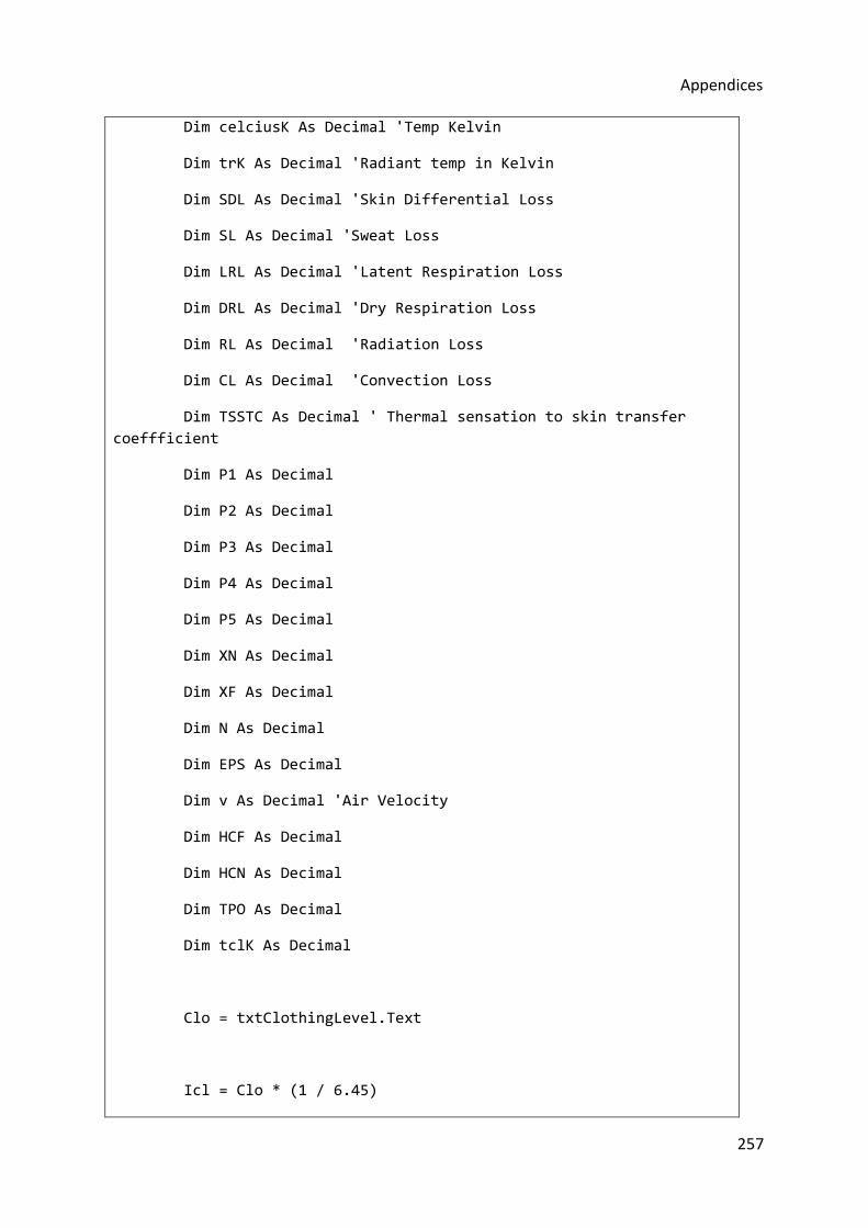
Appendices
257
Dim celciusK As Decimal 'Temp Kelvin
Dim trK As Decimal 'Radiant temp in Kelvin
Dim SDL As Decimal 'Skin Differential Loss
Dim SL As Decimal 'Sweat Loss
Dim LRL As Decimal 'Latent Respiration Loss
Dim DRL As Decimal 'Dry Respiration Loss
Dim RL As Decimal 'Radiation Loss
Dim CL As Decimal 'Convection Loss
Dim TSSTC As Decimal ' Thermal sensation to skin transfer
coeffficient
Dim P1 As Decimal
Dim P2 As Decimal
Dim P3 As Decimal
Dim P4 As Decimal
Dim P5 As Decimal
Dim XN As Decimal
Dim XF As Decimal
Dim N As Decimal
Dim EPS As Decimal
Dim v As Decimal 'Air Velocity
Dim HCF As Decimal
Dim HCN As Decimal
Dim TPO As Decimal
Dim tclK As Decimal
Clo = txtClothingLevel.Text
Icl = Clo * (1 / 6.45)
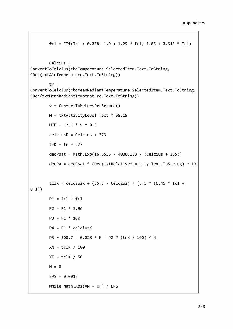
Appendices
258
fcl = IIf(Icl < 0.078, 1.0 + 1.29 * Icl, 1.05 + 0.645 * Icl)
Celcius =
ConvertToCelcius(cboTemperature.SelectedItem.Text.ToString,
CDec(txtAirTemperature.Text.ToString))
tr =
ConvertToCelcius(cboMeanRadiantTemperature.SelectedItem.Text.ToString,
CDec(txtMeanRadiantTemperature.Text.ToString))
v = ConvertToMetersPerSecond()
M = txtActivityLevel.Text * 58.15
HCF = 12.1 * v ^ 0.5
celciusK = Celcius + 273
trK = tr + 273
decPsat = Math.Exp(16.6536 - 4030.183 / (Celcius + 235))
decPa = decPsat * CDec(txtRelativeHumidity.Text.ToString) * 10
tclK = celciusK + (35.5 - Celcius) / (3.5 * (6.45 * Icl +
0.1))
P1 = Icl * fcl
P2 = P1 * 3.96
P3 = P1 * 100
P4 = P1 * celciusK
P5 = 308.7 - 0.028 * M + P2 * (trK / 100) ^ 4
XN = tclK / 100
XF = tclK / 50
N = 0
EPS = 0.0015
While Math.Abs(XN - XF) > EPS

Appendices
259
XF = (XF + XN) / 2
HCF = 12.1 * v ^ 0.5
HCN = 2.38 * Math.Abs(100 * XF - celciusK) ^ 0.25
If HCF > HCN Then
hc = HCF
Else
hc = HCN
End If
XN = (P5 + P4 * hc - P2 * (XF ^ 4)) / (100 + P3 * hc)
N = N + 1
End While
tcl = 100 * XN - 273
SDL = 3.05 * 0.001 * (5733 - 6.99 * M - decPa)
TSSTC = 0.303 * Math.Exp(-0.036 * M) + 0.028
DRL = 0.0014 * M * (34 - TA)
LRL = 1.7 * 0.00001 * M * (5867 - decPa)
CL = fcl * hc * (tcl - Celcius)
RL = 3.96 * fcl * (XN ^ 4 - (trK / 100) ^ 4)
SL = IIf(M > 58.15, 0.42 * (M - 58.15), 0)
If v < 0.2 Then
TPO = 0.5 * Celcius + 0.5 * tr
Else
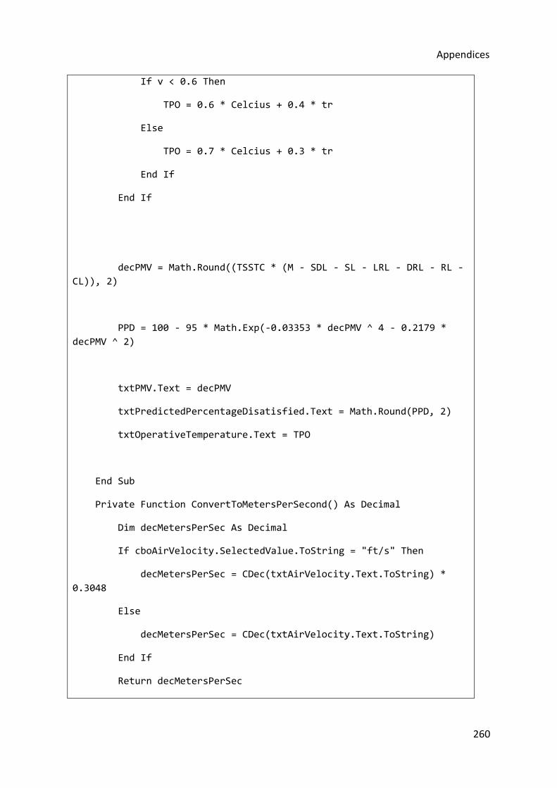
Appendices
260
If v < 0.6 Then
TPO = 0.6 * Celcius + 0.4 * tr
Else
TPO = 0.7 * Celcius + 0.3 * tr
End If
End If
decPMV = Math.Round((TSSTC * (M - SDL - SL - LRL - DRL - RL -
CL)), 2)
PPD = 100 - 95 * Math.Exp(-0.03353 * decPMV ^ 4 - 0.2179 *
decPMV ^ 2)
txtPMV.Text = decPMV
txtPredictedPercentageDisatisfied.Text = Math.Round(PPD, 2)
txtOperativeTemperature.Text = TPO
End Sub
Private Function ConvertToMetersPerSecond() As Decimal
Dim decMetersPerSec As Decimal
If cboAirVelocity.SelectedValue.ToString = "ft/s" Then
decMetersPerSec = CDec(txtAirVelocity.Text.ToString) *
0.3048
Else
decMetersPerSec = CDec(txtAirVelocity.Text.ToString)
End If
Return decMetersPerSec
Appendices
261
End Function
Private Function ConvertToCelcius(ByVal Fahrenheit As String,
ByVal Temp As Decimal) As
Decimal
Dim decFahrenheit As Decimal
If Fahrenheit = "°F" Then
decFahrenheit = (Temp - 32) * 5 / 9
Else
decFahrenheit = Temp
End If
Return decFahrenheit
End Function
Protected Sub Button1_Click(ByVal sender As Object, ByVal e As
System.EventArgs) Handles Button1.Click
PredictedMeanVote()
End Sub
End Class
Appendices
262
Appendix 2 The Indoor Environment Questionnaire
The Indoor Environment Quality Questionnaire
September
20-- The Indoor
Environment Quality Questionnaire

Appendices
263
Background
Five main parameters that affect the quality of the indoor environment have been proposed. They are Thermal comfort, Indoor Air Quality, Acoustic comfort, Lighting, and workplace design. The purpose of this questionnaire is to try and determine how much influence each of the five parameters has on perceived Indoor Environment Quality (IEQ) in offices or related buildings. This will help develop a weighted ranking of the parameters and provide an insight into the complex way in which they combine to dictate perceived IEQ in offices in the UK.
The Questionnaire is divided into two sections:
Section 1 tries to assess, instantaneously, the influence of perceived thermal comfort, indoor air quality, acoustic, visual & workplace design on the overall IEQ during a particular season of the year. [Heating season (November - April) and Cooling season (May - October)]
Section 2 contains personal factors such as age, gender or any underlying problems that could affect your level of satisfaction with the indoor environment. You are not obliged to answer these questions but they may help to explain any discrepancies between field measurements and your subjective opinion.
NB: A guide to answering all questions in section A is provided on a separate sheet, questions in section B are fairly self explanatory. You may use extra space provided for additional comments. Space has been provided at the end of Section 2 if you wish to elaborate on any of the answers you may have given in this questionnaire.
Section 1 - Building Comfort
Please note all the answers should be subjective. For questions in Section 1 please use the assessment scales given and fill in your responses in the spaces provided.
Question 1 - Building characteristics – Please state
Building Name Floor Date Time
Question 2 – The Indoor Environment
(a) Is the Quality of the Indoor Environmental (i.e. IEQ) in this building AT THIS MOMENT acceptable to you? (Please use the assessment scale below):
1 = YES, 0 = NO

Appendices
264
Question 2 – The Indoor Environment
2 (b) How would you rate the quality of Indoor Environment in your work area AT THIS MOMENT ? (Please mark anywhere on the assessment scales below; from 1 to 5)
Question 3 – Thermal Environment
How would you rate your thermal sensation in your work area AT THIS MOMENT ? (Please mark your answer on the assessment scale below)
Cold Cool Slightly Cool
Neutral Slightly Warm
Warm Hot
-3 -2 -1 0 +1 +2 +3
Question 4 – Level of Environment Control
How satisfied are you with your level of control of comfort parameters at your workspace AT THIS MOMENT ? E.g. opening or closing a window or a door to the outside, adjusting a thermostat, drapes or blinds, space heater, turning local fan on or off? (Please mark anywhere on the assessment scale below)
Dissatisfied Slightly
dissatisfied
Slightly
satisfied
Satisfied
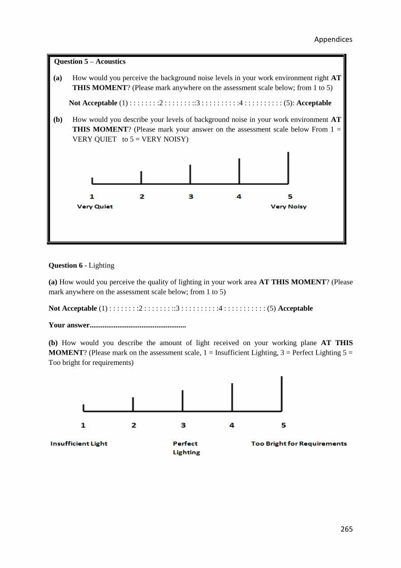
Appendices
265
Question 5 – Acoustics
(a) How would you perceive the background noise levels in your work environment right AT THIS MOMENT ? (Please mark anywhere on the assessment scale below; from 1 to 5)
Not Acceptable (1) : : : : : : : :2 : : : : : : : ::3 : : : : : : : : : :4 : : : : : : : : : : (5): Acceptable
(b) How would you describe your levels of background noise in your work environment AT THIS MOMENT ? (Please mark your answer on the assessment scale below From 1 = VERY QUIET to 5 = VERY NOISY)
Question 6 - Lighting
(a) How would you perceive the quality of lighting in your work area AT THIS MOMENT ? (Please mark anywhere on the assessment scale below; from 1 to 5)
Not Acceptable (1) : : : : : : : :2 : : : : : : : ::3 : : : : : : : : : :4 : : : : : : : : : : : (5) Acceptable
Your answer....................................................
(b) How would you describe the amount of light received on your working plane AT THIS MOMENT ? (Please mark on the assessment scale, 1 = Insufficient Lighting, 3 = Perfect Lighting 5 = Too bright for requirements)

Appendices
266
Question 7 - Indoor Air Quality
(a) How would you perceive the air quality in your work environment AT THIS MOMENT ? (Please mark anywhere on the assessment scale below; from 1 to 5)
Not Acceptable (1) : : : : : : : :2 : : : : : : : ::3 : : : : : : : : : :4 : : : : : : : : : : : (5) Acceptable
(b) How would you describe the levels of air pollution you perceive in your work environment right now? (Please mark your answer on the assessment scale given):
(c) Are you experiencing any of the following symptoms AT THIS MOMENT? (Please tick the scales below at the place that best represents how you feel at this moment)
Blocked nose
Clear nose
Dry nose
Runny nose
Dry throat
Not dry throat
Dry mouth
Not dry mouth
Question 8 - Local Discomfort factors
AT THIS MOMENT do you feel any discomfort caused by any of the following in your work area? Please tick where applicable.
Draughts – cold or warm draughts
Cold floors
Cold equipment
Vertical Air Temperature Varies (e.g. from head to heels)
Discomfort due to differences in radiant heat? e.g. radiators or other heat emitters or surfaces

Appendices
267
Section 2 - Personal Factors
Q1. Please state whether you are Male / Female (circle as appropriate):
Q2. Please state your age category below.
18 – 25 ________
26 – 35 ________
36 – 45 ________
45 – 55 ________
+ 55 ________
Q3. Do you suffer from any physical ailment that might increase your sensitivity to your surrounding environment? For example if you suffer from Reynaud’s disease you may be more sensitive to drops in temperature.
YES / NO
If you have answered yes and are willing to elaborate then please do so in the box below.

Appendices
268
Q4. Further comments on the building’s comfort level are welcomed in the box below. If you wish to elaborate on any of the issues raised in this questionnaire then please refer to the section and question number.
Additional Information:
End of Questionnaire! Thank You for your participation.
NB: Question 3 for Naturally Ventilated Buildings
Cold Cool Neutral Warm Hot
-3 -2 -1 0 +1 +2 +3
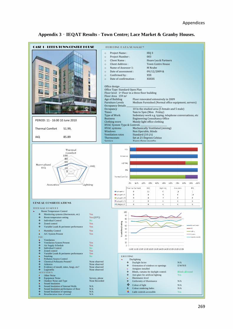
Appendices
269
Appendix 3 IEQAT Results - Town Centre; Lace Market & Granby Houses.
CASE 1 - LEEDS TOWN CENTRE HOUSE BUILDING DATA SUMMARY
RADAR CHART BAR CHART
GENRAL CONSIDERATIONS LINE GRAPH
THERMAL COMFORT
Room Temperature Control Monitoring systems (thermostats, etc) Yes Room temperature setting Yes (21°C) Individual Control No Zoned control Yes Variable Loads & perimeter performance Yes
Humidity Control Yes A/C System Present Yes
IAQ
Ventilation Ventilation System Present Yes Air Supply Schedule Yes Individual Control No Zoned control Yes Variable Loads & perimeter performance Yes
Smoking No Pollution Source Control
Chemical Pollutants Present? None observed Asbestos None observed Evidence of mould, mites, fungi, etc? None observed Legionella None observed ACOUSTICS
Other Noise Equipment Noise Servers, phone Outdoor Noise and Type None Recorded
Sound Insulation Sound Insulation of Internal Walls N/A Sound Insulation performance of floor N/A Sound Insulation of openings N/A Reverberation time of sound N/A
o Project Name : IEQ 3
o Project Number : 003
o Client Name : Hoare Lea & Partners
o Client Address : Town Centre House
o Name of Assessor 1: M Ncube
o Date of assessment : 09/12/2009 &
o Confirmed by : XXX
o Date of confirmation : XXXXX
Office design ___________________________________
Office Type Standard Open Plan
Floor level 1st Floor in a three floor building
Floor Area 159 m2
Age of Building Floor renovated extensively in 2009
Furniture Levels Medium Furnished (Normal office equipment, servers)
Occupancy Details ___________________________________
Occupancy 10 In the studied area (5 female and 5 male)
Times 9am to 5pm (Mon ȂFriday)
Type of Work Sedentary work e.g. typing, telephone conversations, etc
Business Engineering Consultancy Office
Clothing worn Mainly light office clothing
HVAC System Type & Controls __________________________
HVAC systems Mechanically Ventilated (mixing)
Windows Non Operable, blinds
Ventilation rates Standard (10 l/s)
Thermostats Set at 21 Degrees Celsius
Service Every three months
LIGHTING
Daylighting Daylight factor N/A Orientation of windows or openings E/W/N/S
Antiglare installed Blinds, curtains for daylight control: Blinds all round Anti glare for artificial lighting Yes
Illuminance level Uniformity of illuminance N/A
Colour of light N/A Colour rendering Index N/A
Light controls accessible Yes
PERIOD: 11 - 16:00 10 June 2010
Thermal Comfort 51.99,
IAQ 85.89
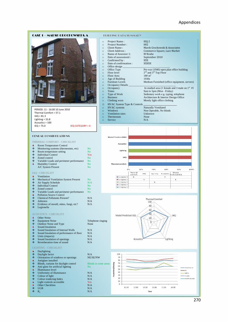
Appendices
270
CASE 1 – MARSH GROCHOWSKI & A BUILDING DATA SUMMARY
GENRAL CONSIDERATIONS
THERMAL COMFORT - CHECKLIST Room Temperature Control
Monitoring systems (thermostats, etc) No Room temperature setting No Individual Control Yes Zoned control No Variable Loads and perimeter performance No
Humidity Control No A/C System Present No
IAQ - CHECKLIST Ventilation
Mechanical Ventilation System Present No Air Supply Schedule N/A Individual Control No Zoned control No Variable Loads and perimeter performance No
Pollution Source Control Chemical Pollutants Present? N/A Asbestos N/A Evidence of mould, mites, fungi, etc? N/A Legionella RADAR CHART
ACOUSTICS - CHECKLIST Other Noise
Equipment Noise Telephone ringing Outdoor Noise and Type None
Sound Insulation Sound Insulation of Internal Walls N/A Sound Insulation of performance of floor N/A Units (impacts) N/A Sound Insulation of openings N/A Reverberation time of sound N/A
LIGHTING - CHECKLIST Daylighting
Daylight factor N/A Orientation of windows or openings NE/SE/NW
Antiglare installed Blinds, curtains for daylight control Blinds in some areas Anti glare for artificial lighting No
Illuminance level Uniformity of illuminance N/A Colour of light N/A Colour rendering Index N/A
Light controls accessible Yes Other Checklists N/A
UGR N/A Ra N/A
o Project Name : IEQ 2
o Project Number : 002
o Client Name : Marsh Grochowski & Associates
o Client Address : Commerce Square, Lace Market
o Name of Assessor 1: M Ncube
o Date of assessment : September 2010
o Confirmed by : XXX
o Date of confirmation : XXXXX
o Office design ___________________________________ o Office Type Pre-war (1940) open plan office building o Floor level 2nd and 3rd Top Floor o Floor Area 180 m2 o Age of Building 1930s o Furniture Levels Medium Furnished (office equipment, servers) o Occupancy Details ___________________________________ o Occupancy In studied area (1 female and 3 male on 1st Fl o Times 9am to 5pm (Mon –Friday) o Type of Work Sedentary work e.g. typing, telephone o Business Architecture & Interior Design Office o Clothing worn Mostly light office clothing
o HVAC System Type & Controls __________________________ o HVAC systems Naturally Ventilated o Windows Non Operable, No blinds o Ventilation rates Unknown o Thermostats None o Service N/A
PERIOD: 11 - 16:00 10 June 2010
Thermal Comfort = 57.1
IAQ = 81.3
Lighting = 55.8
Acoustics = 100
IEQ = 75.0 IEQ CATEGORY = II
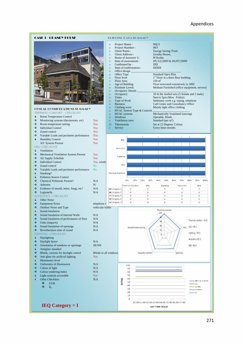
Appendices
271
CASE 1 - GRANBY HOUSE BUILDING DATA SUMMARY
GENRAL CONSIDERATIONS SUMMARY
THERMAL COMFORT - CHECKLIST Room Temperature Control
Monitoring systems (thermostats, etc) Yes Room temperature setting Yes Individual Control Yes Zoned control Yes Variable Loads and perimeter performance Yes
Humidity Control Yes A/C System Present Yes
IAQ - CHECKLIST Ventilation
Mechanical Ventilation System Present Yes Air Supply Schedule Yes Individual Control Yes, windows operable Zoned control No Variable Loads and perimeter performance No
Smoking* Pollution Source Control
Chemical Pollutants Present? N/A RADAR CHART Asbestos N/ Evidence of mould, mites, fungi, etc? N/A Legionella N/A ACOUSTICS - CHECKLIST
Other Noise Equipment Noise telephone ringing Outdoor Noise and Type vehicular traffic
Sound Insulation Sound Insulation of Internal Walls N/A Sound Insulation of performance of floor N/A Units (impacts) N/A Sound Insulation of openings N/A Reverberation time of sound N/A LIGHTING - CHECKLIST
Daylighting Daylight factor N/A Orientation of windows or openings SE/SW
Antiglare installed Blinds, curtains for daylight control Blinds in all windows Anti glare for artificial lighting Yes
Illuminance level Uniformity of illuminance N/A Colour of light N/A Colour rendering Index N/A
Light controls accessible Yes Other Checklists N/A
UGR Ra
IEQ Category = I
o Project Name : IEQ 3
o Project Number : 003
o Client Name : Energy Saving Trust
o Client Address : Granby House,
o Name of Assessor 1: M Ncube
o Date of assessment : 09/12/2009 & 20/07/2009
o Confirmed by : XXX
o Date of confirmation : XXXXX
o Office design ___________________________________ o Office Type Standard Open Plan o Floor level 1st Floor in a three floor building o Floor Area 159 m2 o Age of Building Floor renovated extensively in 2009 o Furniture Levels Medium Furnished (office equipment, servers) o Occupancy Details ___________________________________ o Occupancy 10 In the studied area (5 female and 5 male) o Times 9am to 5pm (Mon –Friday) o Type of Work Sedentary work e.g. typing, telephone o Business Call Centre and Consultancy Office o Clothing worn Mainly light office clothing o HVAC System Type & Controls __________________________ o HVAC systems Mechanically Ventilated (mixing) o Windows Operable, blinds o Ventilation rates Standard (per m2) o Thermostats Set at 22 Degrees Celsius o Service Every three months
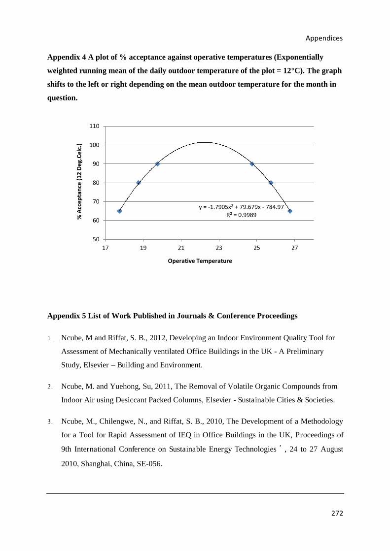
Appendices
272
Appendix 4 A plot of % acceptance against operative temperatures (Exponentially
weighted running mean of the daily outdoor temperature of the plot = 12°C). The graph
shifts to the left or right depending on the mean outdoor temperature for the month in
question.
Appendix 5 List of Work Published in Journals & Conference Proceedings
1. Ncube, M and Riffat, S. B., 2012, Developing an Indoor Environment Quality Tool for
Assessment of Mechanically ventilated Office Buildings in the UK - A Preliminary
Study, Elsevier – Building and Environment.
2. Ncube, M. and Yuehong, Su, 2011, The Removal of Volatile Organic Compounds from
Indoor Air using Desiccant Packed Columns, Elsevier - Sustainable Cities & Societies.
3. Ncube, M., Chilengwe, N., and Riffat, S. B., 2010, The Development of a Methodology
for a Tool for Rapid Assessment of IEQ in Office Buildings in the UK, Proceedings of
9th International Conference on Sustainable Energy Technologies, 24 to 27 August
2010, Shanghai, China, SE-056.
y = -1.7905x2 + 79.679x - 784.97
R² = 0.9989
50
60
70
80
90
100
110
17 19 21 23 25 27
% A
cce
pta
nce
(1
2 D
eg
.Ce
lc.)
Operative Temperature