1

Near-Field Acoustic Holography: The Frame Drum

Grégoire Tronel

University of Illinois Urbana-Champaign

Summer REU – 2010 Advisor: Dr Steven Errede

__________________________________________

Abstract A phase-sensitive setup for near-field acoustic holography was established in order to determine the characteristic resonance modes of a vibrating membrane. The experiment was carried out using a frame drum as the vibrating system of interest. By exciting the membrane at certain fundamental frequencies and recording the complex signals from the pressure and particle velocity fields across the drumhead, we modeled 3-D representations of the vibrating surface. Correlations between an eigen-frequency and its corresponding eigen-mode of resonance are described throughout this report.

Introduction and Theoretical Description A percussion instrument played by striking a tightly stretched membrane attached to a circular frame is called a membranophone. The transient nature of its sound reveals tones with non-periodic waveforms which will therefore have non-harmonic partials and pitches more or less indeterminate. To understand and represent such unique acoustical behavior, we conducted our experimental work using a frame drum as the vibrating system of interest. For a circular membrane with no displacement at the boundary, the ideal vibrational model is well known and can be derived mathematically.

( ) ( ) ( ) ( )rtiXtrXtv

trX 202

2

22 exp,,1.,, δωφφ =

∂∂

−∇

This is the expression corresponding to the membrane motion where X is the displacement of the membrane from its rest position, v is the velocity, ω is the angular frequency, r is the position along the radius and φ is the angle to the x-axis. The left hand

2

side of the equation describes a point like perturbation that oscillates with frequency positioned at r = 0 ( ( )rδ is a two-dimensional delta-function with dimension 1/r2). Hence looking at r different than 0, the equation for the displacement becomes:

( ) ( ) 0,,1.,, 2

2

22 =

∂∂

−∇ trXtv

trX φφ [i]

Where the Laplacian operator 2∇ for a two dimensional problem is given by

2

2

22 11

φ∂∂

+⎟⎠⎞

⎜⎝⎛

∂∂

∂∂

=∇rr

rrr

.

Inserting the Laplacian into [i],

( ) ( ) 0,,1.,,112

2

22

2

22

2

=∂∂

−⎥⎦

⎤⎢⎣

⎡∂∂

+∂∂

+∂∂ trX

tvtrX

rrrrφφ

φ

Assuming ( ) ( ) )(,,, tTrXtrX φφ = where T(t) = exp(iω t), we obtain a time independent equation:

( ) ( ) 0,.,112

2

2

2

22

2

=+⎥⎦

⎤⎢⎣

⎡∂∂

+∂∂

+∂∂ φωφ

φrX

vrX

rrrr

Making the following separation of variables ( ) ( ) ( )φθ PrRrX =, , the equation becomes:

( ) ( ) ( ) ( ) 0112

22

2

2

2

22 =+

∂∂

+⎥⎦

⎤⎢⎣

⎡∂∂

+∂∂

vrP

PrR

rr

rr

rRωφ

φφ.

The φ dependency is equal to a constant; thus we can separate the r and φ terms into two distinct differential equations:

( ) ( )

( ) ( )

2 22

2 2

22

2

1 mR r k R rr r r r

P m Pφ φφ

⎡ ⎤ ⎛ ⎞∂ ∂+ = −⎜ ⎟⎢ ⎥∂ ∂⎣ ⎦ ⎝ ⎠∂

= −∂

With v = f λ = (ω/2π)(2π/k) = ω/k. Solving the equation for P(φ ):

( ) ( ) ( ) …,2,1,0sincos ±±=+= mmmP mm φβφαφ .

3

αm and βm are arbitrary constants which satisfy the following condition: 122 =+ mm βα .

Now looking at ( )rR :

( ) ( ) 012

22

2

2

=⎟⎟⎠

⎞⎜⎜⎝

⎛−−⎥

⎦

⎤⎢⎣

⎡∂∂

+∂∂ rR

rmkrR

rrr

This equation is called the Bessel equation, named after the German mathematician Friedrich Wilhelm Bessel, the solution is of the form:

( ) ( ) ( )krYBkrJArR mmmm += Where Jm(kr) and Ym(kr) are Bessel functions of the 1st and 2nd kind respectively. Although for our purpose, Ym cannot be a solution due to the fact that it diverges when r approaches 0. Therefore Bm= 0 (we ignore the Bessel functions of the 2nd kind). Jm has to vanish on the edge (boundary) of the membrane meaning that Jm(x=kR)= 0, where R is the radius of the drum. As figure 1 shows us, there are multiple points where Jm equals zero. The radius of the membrane being constant, there exist an infinite number of different k-vectors that satisfy the boundary condition. We name those km,n where n corresponds to the nth zero of Jm. Graphically, m refers to the order number of a Bessel function and n represents the number of nodes. Note that the above derivation was partly taken from Dr Errede’s lecture notes {1}. We have now sufficient information to obtain the eigen-mode solutions for X(r,φ ,t): The eigen-mode solution of the temporal wave equation is of the following form(s):

Figure 1: Bessel functions of the 1st and 2nd kind. To the left, the first five Bessel functions of the 1st kind (Jm) are shown. The right figure shows the first five Bessel functions of the 2nd kind (Ym). Note that Ym diverges as r approaches zero.

( )

( )( ) )](exp[

)cos()sin(

1 ; 11 ; 11

)cos()sin(

,,,

,,,,,

2,

2,,,

,,,,,

nmnmnm

nmnmnmnmnm

nmnmnmnm

nmnmnmnmnm

titTtttT

cbcb

tctbtT

φωφωδω

ωω

+=

+=+=

=++≤≤−+≤≤−

+=

4

The complete eigen-mode solution for the two-dimensional standing wave on a 2-D circular membrane is thus given by:

( )( )( ) )]sin()cos()][sin()cos()[(,,

)](exp[)](exp[)(,,)()()(,,

,,,,,,,.

,,,,,,.

,,.

tctbmmRkJAtrXtimiRkJAtrX

tTPrRtrX

nmnmnmnmmnmnmnmnm

nmnmnmnmnmnmnm

nmmnmnm

ωωφβφαφφωδφφ

φφ

++=

++=

=

With eigen-frequencies, eigen-wavelengths and eigen-energies of:

f m ,n = ω m ,n /2π = vk m ,n /2π = v /λm ,n

λm ,n = 2π / km ,n = 2πR / x m ,n

E m ,n =14

Mω m ,n2 Am ,n

2

m = 0,1,2,3... and n = 0,1,2,3....

In the complete solution, Am,n corresponds to the amplitude arbitrarily determined by the function generator. Note that if we excite the drumhead at r = 0, we can only generate the modal vibrations which possess an anti-node at this point. In order to generate other eigen-modes, one has to move the position where the driven force acts to r = d, a distance along the radius. Note that all J0 modes are non degenerate whereas all the other modes (m > 0) possess 2-folds degeneracies, because of the two spatial degrees of freedom (x-y or r-φ ) and the rotational symmetry of the circular membrane. The following expression helps finding the (ideal) eigen-frequency that one must apply to the drumhead in order to reveal one specific normal mode (although different from our experimental method of finding eigen-frequencies):

ππω

ν22

,,,

nmnmnm

vk==

Once an eigen-frequency is known, we can examine the complex sound field by calculations of the pressure and particle velocity fields associated to it. The complex particle velocity ( ),u r t (a 3D complex vector quantity) is derived from the

complex pressure ( ),p r t (a complex scalar quantity) via Euler’s equation for inviscid fluid flow:

( ) ( ), 1 ,o

u r tp r t

t ρ∂

= − ∇∂

[ii]

5

In cylindrical/polar coordinates: 1ˆ ˆ zz

ρ ϕρ ρ ϕ∂ ∂ ∂

∇ = + +∂ ∂ ∂

where 2 2x yρ = + ,

( )1tan y xϕ −= and ˆ ˆ ˆcos sinx yρ ϕ ϕ= + , ˆ ˆ ˆsin cosx yϕ ϕ ϕ= − + . For a complex harmonic sound field, the complex pressure eigen-functions (at z = 0) associated with the modal vibrations of an ideal (i.e. perfectly compliant) drum membrane of radius R, are solutions to the 3D wave equation for the complex pressure

( ) ( ) ( )2 2 2 2, 1 , 0p r t v p r t tφ∇ − ∂ ∂ = (phase velocity v kφ ω= ) and are of the general form:

( ) ( ) ( ) ( )

( ) ( ) ( )

, ,

,

, , 0, cos

cos

ii t k zm n o m m n o

ii t k zo m m n o

pz

pz

p z t p J k m e e

p J R m e e

ϕω

ϕω

ρ ϕ ρ ϕ ϕ

ξ ρ ϕ ϕ

−

−

= = − ⋅ ⋅

= − ⋅ ⋅

Where ,m nk is the radial wave-number for the ( ), thm n mode, denoting the ( ), thm n zero

( , ,m n m nk Rξ ≡ ) of the Bessel function ( ), 0m m nJ ξ = at the radial boundary Rρ = and oϕ is the rotation angle about the z-axis of the entire distribution in the x-y plane, defined by the x-y location of the driving force point. Then to find the particle velocity from [ii],

( ) ( ) ( ) ( )

( ) ( ) ( )

, ,

,

1ˆ ˆ ˆ, , 0, cos

1ˆ ˆ ˆ cos

ii t k zm n o m m n o

ii t k zo m m n o

pz

pz

p z t z p J k m e ez

z p J R m e ez

ϕω

ϕω

ρ ϕ ρ ϕ ρ ϕ ϕρ ρ ϕ

ρ ϕ ξ ρ ϕ ϕρ ρ ϕ

−

−

⎧ ⎫∂ ∂ ∂∇ = = + + − ⋅ ⋅⎨ ⎬∂ ∂ ∂⎩ ⎭

⎧ ⎫∂ ∂ ∂= + + − ⋅ ⋅⎨ ⎬∂ ∂ ∂⎩ ⎭

Now,

( ) ( ) ( ){ }1, , 1 , 1 ,2m m n m n m m n m m nJ k k J k J kρ ρ ρ

ρ − +∂

= −∂

and for m = 0: ( ) ( )0 0, 0, 1 0,n n nJ k k J kρ ρρ∂

= −∂

, ( ) ( )cos sino om m mϕ ϕ ϕ ϕϕ∂

− = − −∂

,

z zik z ik zze ik e

z− −∂

= −∂

Hence for a harmonic sound field:

( ) ( ) ( ) ( ) ( ),,

i t i to i t

o o

u r t u r e eu r i u r e i u r tt t t

ω ωωω ω

∂ ∂ ∂= = = =

∂ ∂ ∂.

Thus, the radial, angular and height components of the complex particle velocity are found to be:

6

( ) ( ) ( ){ } ( ) ( ),, 1 , 1 ,, , 0, cos

2ii t k zm n o

m n m m n m m n oo

pzk p

u z t J k J k m e ei

ϕωρ ρ ϕ ρ ρ ϕ ϕωρ

−− += = − − − ⋅ ⋅

( ) ( ) ( ) ( ), ,, , 0, sin ii t k zo

m n m m n oo

pzmpu z t J k m e ei

ϕωϕ ρρ ϕ ρ ϕ ϕωρ

−= = + − ⋅ ⋅

( ) ( ) ( ) ( ), ,, , 0, cos ii t k zz z o

m n m m n oo

pzk pu z t J k m e e ϕωρ ϕ ρ ϕ ϕωρ

−= = + − ⋅ ⋅

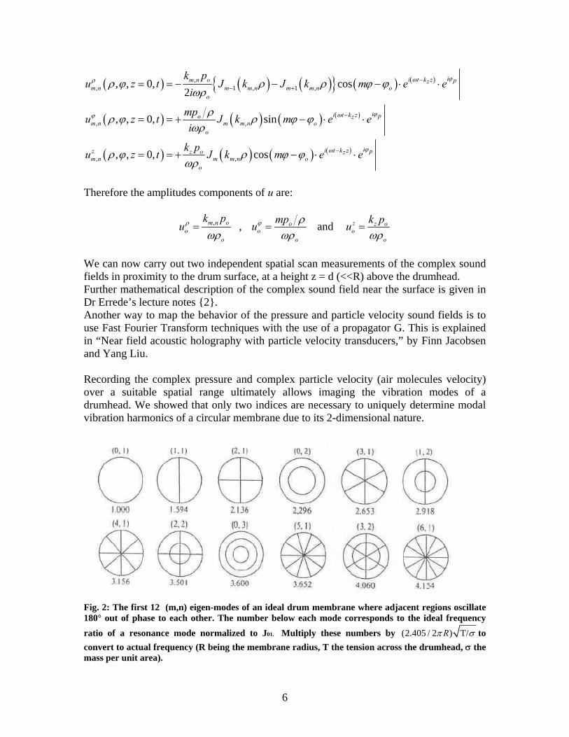
Therefore the amplitudes components of u are:

,m n o

oo

k puρ

ωρ= , o

oo

mpuϕ ρωρ

= and z z oo

o

k puωρ

=

We can now carry out two independent spatial scan measurements of the complex sound fields in proximity to the drum surface, at a height z = d (<<R) above the drumhead. Further mathematical description of the complex sound field near the surface is given in Dr Errede’s lecture notes {2}. Another way to map the behavior of the pressure and particle velocity sound fields is to use Fast Fourier Transform techniques with the use of a propagator G. This is explained in “Near field acoustic holography with particle velocity transducers,” by Finn Jacobsen and Yang Liu. Recording the complex pressure and complex particle velocity (air molecules velocity) over a suitable spatial range ultimately allows imaging the vibration modes of a drumhead. We showed that only two indices are necessary to uniquely determine modal vibration harmonics of a circular membrane due to its 2-dimensional nature.

Fig. 2: The first 12 (m,n) eigen-modes of an ideal drum membrane where adjacent regions oscillate 180° out of phase to each other. The number below each mode corresponds to the ideal frequency ratio of a resonance mode normalized to J01. Multiply these numbers by (2.405 / 2 ) T/Rπ σ to convert to actual frequency (R being the membrane radius, T the tension across the drumhead, σ the mass per unit area).

7

We clearly see that the harmonic spectrum of a drum (and percussions in general) differs from almost every other instrument whose harmonics are integer multiples of the lowest resonance mode (fundamental frequency). These frequency-related phenomena are well described by T.D. Rossing in “The Physics of Musical Instruments” (1973) {3}.

Many other physical quantities may be derived from the spatial measurements of the complex pressure and complex particle velocity fields near the vibrating membrane.

Among those are the complex acoustic impedance (~~~

/UPZ = ), the complex sound

intensity (~~~*.UPI = ), as well as structural wave number indications and phase

information. An insightful description of these many physical quantities is given in Dr Errede’s lecture notes {4}.

Apparatus and Experimental Procedure

The extraction of fundamental acoustic quantities such as the complex pressure and complex particle velocity is crucial for a profound understanding of a complex acoustic sound field and leads to an accurate 3-D representation of a non-ideal vibrating system. In order to track such acoustic phenomena, a specific data-acquisition (DAQ) system was established. It describes a phase sensitive setup for near-field acoustic holography (NAH).

Fig.3: Picture taken inside the lab showing the DAQ system for acoustic holography.

Computer for data processing

Lock-in Amplifiers

Thompson rods - Motorized translational stages

Pressure and particle velocity microphones (above and below the drum)

Frame drum

8

Two small super-magnets (earth magnets) are positioned above and below the drum membrane at a desired position. A function generator is used to drive a sinusoidal current to a coil situated beneath the magnets. An existing negative impedance circuit (NIC) takes the flat (frequency-related) current output to a stable input power level. It ensures a constant magnetic field to drive the magnets. Note that the constant current NIC eliminates phase shifts (time delayed response of the drumhead from its driven force) due to inductance of the coil. The current running through the coil induces an oscillatory magnetic field which causes the magnets to move up and down, producing vibrations across the drumhead, for any input frequency. Two pairs of pressure and particle velocity microphones situated above and below the drum membrane are used to extract the acoustical quantities needed to understand and characterize the sound field and vibrational behavior of the drumhead. To extract such physical quantities from the microphones, each microphone was absolutely calibrated in a Lp = 94.0 dB sound field at f = 1 KHz, using a NIST-certified Extech 40774 calibrator. Upon calibration their output voltage could then be related to either pressure or particle velocity (expressed in RMS Pa or mm/s, rather than arbitrary RMS volts). [In a Lp = 94.0 dB sound field @ NTP: |p| = 1.0 Pa (RMS) and |u| = 2.42 mm/s (RMS)]. The pressure and particle velocity microphones that are placed above the drumhead are called the “scan mics” because they are attached to the motorized and computerized translational stages in order to spatially scan the entire drumhead surface by making 32x32 measurements with 1cm steps. These stages called Thompson rods are accurate to a micrometer. The microphones placed underneath the drumhead (“monitor mics”) hold a different purpose. Because vibrating systems such as a circular membrane have a notable dependence to weather-related quantities such as the temperature, humidity and atmospheric pressure, a mode-locking system had to be established in order to keep track of the resonant frequency (=fcn(T,P,H)) using digital-techniques in the PC’s DAQ code. Therefore, a pair of pressure and particle velocity microphones was positioned below the membrane to mode-lock to a desired resonant frequency, holding the phase for the pressure monitor microphone constant at 90.0+_0.5 degrees. When the drum vibrates at an eigen-mode, the pressure beneath the magnets is at a maximum and entirely imaginary. To access a desired eigen-mode of vibration, the frequency is swept until the pressure in the complex plane is aligned with the positive or negative imaginary axis depending on the pre-defined parity of the magnets. The complex signal from each microphone is sent to a Lock-in Amplifier (thus four LIA’s). Each LIA measures the amplitudes of the real/in-phase and imaginary/90°-out-of-phase components of a complex harmonic (i.e. periodic) signal, both relative to stable sine wave of reference. More theoretical description of LIA’s is given in Dr Errede’s lecture notes {5}. Ultimately, the recorded complex signals for each measurement and all the phase information obtained through data acquisition is processed by a computer. Note that the real part of the sound field relates to the sound that propagates to one’s ear, decaying through time, whereas the imaginary part corresponds to oscillatory vibrations near the drum surface. The known phase-shifts effects (which we’ll discuss later) are corrected in the offline data analysis. As stated in the theory, only certain modes may be generated depending on where the drumhead is being excited, and at which frequency are the magnets driven (i.e. frequency

9

at which the drumhead is vibrating). However, characteristic modes of vibration can only be observable if the membrane vibrates at an eigen-frequency. Hence the first step of the experimental procedure is called a frequency scan. The purpose is to maintain the scan microphones at constant position above the magnets and then sweep the frequency over a pre-defined range. For our motif, we chose the frequency scan to go from 0.5 Hz to around 2 kHz with 1 Hz steps. Although most of what appears interesting and relevant occurs between ~100 Hz and ~800 Hz. We conducted three frequency scans at the center, half radius, and edge of the drum (each scan lasts about four hours). By then analyzing the recorded pressure spectrum over the given range of frequencies and distinguishing the local maxima of pressure, one can quickly identify the resonance peaks of the drumhead, each peak corresponding to an eigen-frequency for this driving force position. The second part consists of a spatial scan. It is what permits us to image the vibration modes (eigen-modes) of the drum membrane. Once the eigen-frequencies are known, one can stabilize the magnet vibrations to a desired frequency, exciting the drumhead at its corresponding mode of resonance. Then the translational stages supporting the P/U microphones will scan the drumhead (as previously described) allowing 3D representation of the vibrating system and revealing the relation between a Jmn eigen-mode and its eigen-frequency. The following figures display 3-D plots of the first 12 eigen-modes for a perfectly compliant membrane. These Jmn Bessel functions form the harmonic spectrum of all vibrating circular membranophones. An ideal modeling of these normal modes is shown below, where the first column represents (0,n) modes and the first row (m,1) modes etc...:

10

Investigation of a Frame Drum - Results and Analysis The object of interest is a 12 inches frame drum made by Remo with synthetic calfskin called “fiberskyn 3”. Its membrane is made out of two layers (PET film and Tyvek) jointed to the wooden frame by a nylon web strip. The frame drum surface was positioned at about 4mm above and below the monitor and scan microphones respectively. Note that due to the emplacement of the coil right underneath the magnets, the monitor microphones were placed on each side of the coil, adding distance from the microphones to the driving force position. As stated in the experimental procedure, a frequency scan has first been carried out. The purpose is to find the constructive and destructive interference patterns between the function generator input frequencies and the drumhead response. The theory informs that only certain modes are accessible depending on where is situated the driving force point. Therefore we chose to conduct a frequency scan at three different positions along the radius of the drum membrane.

Fig.4: Frequency scan performed at the center of the drumhead. It shows the RMS values for the pressure (left) and particle velocity (right) amplitudes. Amplitudes of the pressure and particle velocity fields indicate where the interferences occur. The positive peaks denoted by circles designate resonance modes. Resonance can be characterized by the tendency of an acoustic system to absorb more energy when it is driven at a frequency that matches one of its own eigen-frequency of vibration (i.e. resonant frequency). Each positive peak can be related to an eigen-mode of vibration. Since the membrane was first driven at the center, one may quickly conclude that the three first peaks displayed on the graph probably refer to the three first (0,n) modes, respectively J01 (176.7 Hz), J02 (426.2 Hz) and J03 (662.6 Hz). Note that two frequencies of resonance that are very close to each other may generate a combination of two distinct eigen-modes if the membrane is being driven at one of these frequencies. Having two

11

close-by eigen-frequencies is probably due to the fact that the drumhead possesses a finite stiffness (i.e. not perfectly compliant). As mentioned in the previous section, the next step is to stabilize the driving force at a frequency of interest. The first frequency peak was found to be 176.7 Hz. Before starting a spatial scan of the first eigen-mode at this frequency, room conditions were also recorded: T the voltage amplitude of the function generator was 4.0 V, the LIA’s sensitivity was 1000 mV, the ambient temperature was 20.7°C, the relative humidity 63% and the atmospheric pressure 740 mmHg. Variations in these weather dependant quantities strongly influence the resonant frequency. The following graphs provide information about the drifting eigen-frequency and the reference phase for the magnets positioned at the center of the drum.

Fig.5: The left picture represents the drifting resonant frequency and the right picture shows the reference phase (with a negative parity), both in function of the measurement number (32x32). The final room temperature was recorded to be 23.3°C, (2.6°C warmer than when the scan started). Note that for a low mode such as J01, it takes about 4 hours to complete a spatial scan. The left graph reveals that the eigen-frequency is being slightly shifted during the scan period. The drift in ambient temperature is principally responsible for shifting the eigen-frequency; however the use of the mode-locking monitor microphones allows keeping track of the resonant mode of vibration. The reference phase was roughly locked between -88° and -90°. For an ideal membrane, the frequency and phase would be constant throughout the entire scan period. The next step is the modal analysis, which I recall, is the process of describing the dynamic properties of an elastic structure in terms of its eigen-modes of vibration. Once a spatial scan is done, one can obtain 3-D representations of many acoustical quantities relevant to our study. Distribution of the complex pressure and the complex particle velocity across the drum surface provide insightful information about the excited normal mode.

12

Fig.6: 3-D representation of the imaginary parts of the pressure (left) and particle velocity (right) obtained through scanning the entire drum surface with a driven frequency of roughly 176 Hz. The excitation point (i.e. magnets position) is at the center of the drum. One can immediately conclude that the first obtained eigen-frequency corresponds to the J01 eigen-mode also called “breathing mode”, which is the lowest resonance mode for a circular vibrating system. Note that all the recorded amplitudes throughout this report are root-mean-squared (RMS) values. Many other representations of complex acoustical quantities (particle displacement and acceleration, acoustic impendence, sound intensity and power, energy density, linear and angular momentum densities, phase information…) may be obtained through offline data analysis from the measured pressure and particle velocity fields. An image representation was constituted through scanning the vibrating surface at a desired mode-locked eigen-frequency. Figure 4 showed the first positive frequency peak to be related to the first eigen-mode of vibration. The next two maxima might also reveal new eigen-modes of higher order. During this second spatial scan, we had to lower the LIA’s sensitivities and the voltage amplitude of the function generator to 1.5 V to prevent the scan from overloading and stopping. Phase offsets were found to be +58° for the monitor microphones, -31° for the pressure and -26° for the particle velocity scan microphones. These phase corrections are added to the raw data in the offline analysis. Although carefully recorded, room conditions and LIA’s sensitivities for the remaining modes will not be listed throughout the rest of the analysis.

13

Fig.7: Same plots as Fig.5, for a mode-locked eigen-frequency of roughly 426.2 Hz (+/- 0.5 Hz). The reference phase is locked around the desired -90° (negative parity). According to the theoretical explanation, one would expect this mode of resonance to be the second (0,n) mode or J02. The frequency ratio of this mode normalized to J02 is about 2.41, which seems closer to the expected theoretical ratio of 2.296.Taking a closer look at the pressure and particle velocity repartitions:

14

Fig.8: Left are the real parts of the pressure (top) and particle velocity (bottom). Their imaginary parts are displayed on the right hand side. The spatial scan for the second eigen-frequency of 426.2 Hz reveals disturbing results. Even though we exclusively expected the second eigen-mode to be a (0,n) mode due the excitation being at the center of the drum, the top and bottom left plots clearly shows that the mode displayed isn’t J02 but J21. However, the imaginary components (right) of the pressure and particle velocity fields show considerable resemblance with the J02 eigen-mode. Thus it seems both modes are being generated at a frequency of roughly 426 Hz. The reason why we were also able to excite the drum at its J21 eigen-mode is due to the fact that two nearby frequencies of resonance are close enough to each other so that both of the eigen-modes are being excited at the same time. A probable cause for such artifact is that the drum membrane is not perfectly compliant. More information about the principal resonance-shift effects due to a non-ideal system is given in The Physics of Musical Instruments by Fletcher and Rossing {3}. The next frequency peak shown in figure 4 is at 662.6 Hz. The corresponding expected eigen-mode should be J03., although the frequency ration is 3.75 which is closer to the J51

mode if we consider the theoretical ratios.

Fig.9: Imaginary pressure (left) and particle velocity (right) for a frequency locked around 662 Hz.

15

As theoretically expected, the displayed resonance mode which corresponds to the eigen-frequency of 662 Hz is the J03 Bessel function. Although one may notice that the amplitude of the outer ring is not homogenous along its perimeter. It is divided into four lumps of similar amplitudes which is an artifact of the J22 Bessel function. The J22 mode should not be directly excited when the driving force is placed at the center because it possesses a node at this point. Its theoretical frequency ratio is 3.501, close to the ratio of 3.600 of the J03 mode. These two eigen-modes are presumably very close each other and are being generated simultaneously when driven around 662 Hz. Once again a probable cause for such artifact is due to the finite stiffness of the membrane (as previously mentioned in the analysis of the previous mode at 426 Hz). For a clearer interpretation of the resonant frequencies, we plotted the results of three frequency scans at different magnets positions along the drum radius:

Fig.10: Frequency scan for three different positions of the driven force: At the center (blue - same as figure 4), half-radius (green) and at the edge (red). As previously stated, one should be able to excite the drumhead at only certain modes of vibration depending on where the membrane is being excited. A plot of the pressure amplitudes for different magnets positions may help us not to unnecessarily waste time. If one looks at the green curve, the prominent positive peaks (below ~700Hz) sensibly overlap with peaks of the red curve. However the red curve possesses maxima which do not overlap with those from the other curves. Therefore, only five more spatial scans are necessary to cover the frame drum harmonic spectrum for the frequency range of interest (< 700 Hz). Note that after 700 Hz, protuberant artifacts of the system such as shell resonance may alter the accuracy and clarity in characterizing an eigen-mode. Whereas below 100 Hz, noise due to the machinery and the ventilation system seem to dominate the microphones signal.

16

Five spatial scans were then performed at 309.5 Hz, 520 Hz, 575 Hz, 615 Hz and 685 Hz (positive peaks of the red curves corresponding to yet unknown modes). Note that these frequencies are just starting values and are more or less approximate due to the influence of climate conditions as described earlier. Eigen-modes generated by these five frequencies can all be excited by positioning the driving force at the edge of the drum membrane (12.5 cm from the center).

Fig.11: 3-D plot of the imaginary pressure (top-left), imaginary particle velocity (bottom-left), real pressure (top-right) and real particle velocity (bottom-right). The magnets were positioned at the edge of the drumhead and initially driven at about 309.5 Hz. The eigen-mode that corresponds to a frequency of approximately 309.5 Hz is undeniably the J11 eigen-mode. The frequency ratio is 1.75, relatively close to the theoretical ratio of 1.59. A lump on the +y anti-node shows a default in the curve smoothness. This lump coincides with the point where the membrane is being driven. The magnets position also coincides with the quarter of the drum that does not possess a supporting clamping arm (which damps acoustical energy out of the system). Taking a closer look at the real components of the pressure and particle velocity fields, we observe an orthogonal rotation of the structure in the x-y plane. The imaginary distributions possess a nodal line in the x-direction whereas it has been shifted in the y-direction for the real parts.

17

The next frequency of interest is about 520 Hz. The imaginary distribution obtain from the spatial scan is shown below in figure 12. The resemblance with the J13 eigen-mode is significant enough to conclude that this resonant mode is well defined at this input frequency and no coupling of two nearby modes took place.

Fig.12: Imaginary part of the pressure (left) and particle velocity (right). The magnets are at the edge and the driving frequency is roughly locked around 520 Hz. The three remaining frequencies (575 Hz, 615 Hz and 685 Hz) unexpectedly correlate to unclear combinations of two nearby modes of resonance. The following graphs display the imaginary part of the pressure and particle velocity fields.

Fig.13: Vibration mode of the drumhead when driven at 575 Hz.

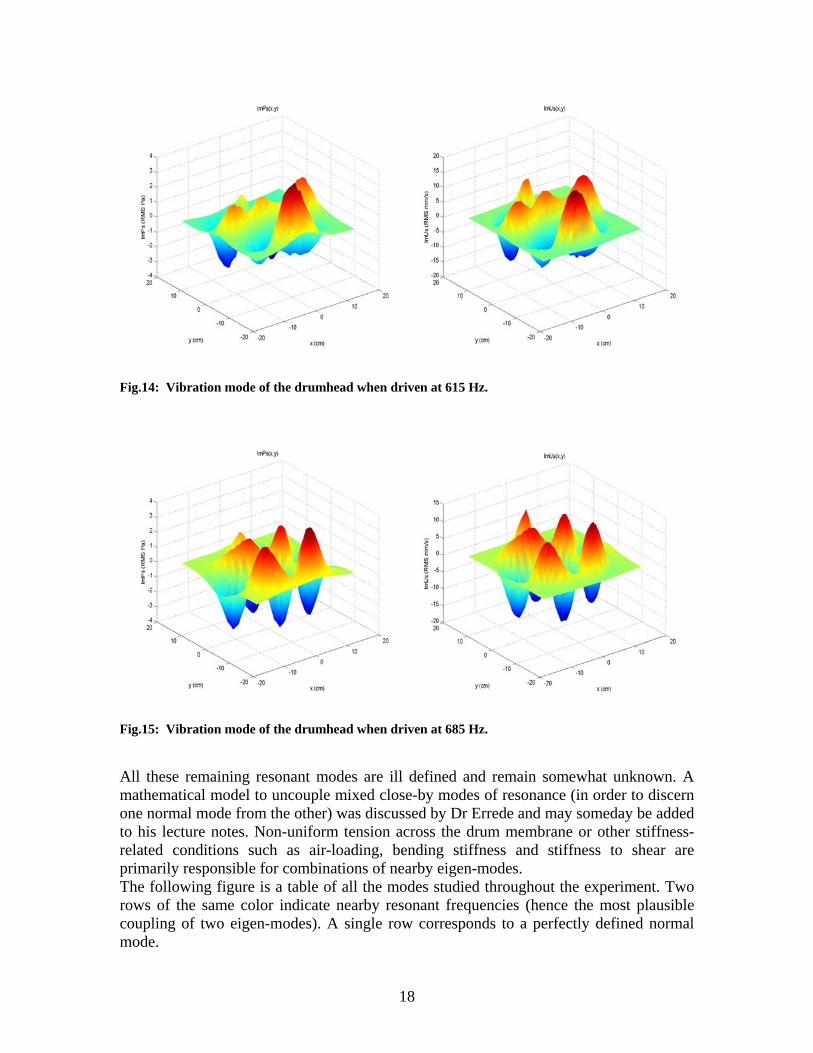
18

Fig.14: Vibration mode of the drumhead when driven at 615 Hz.

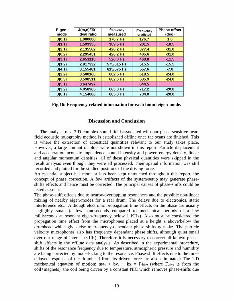
Fig.15: Vibration mode of the drumhead when driven at 685 Hz. All these remaining resonant modes are ill defined and remain somewhat unknown. A mathematical model to uncouple mixed close-by modes of resonance (in order to discern one normal mode from the other) was discussed by Dr Errede and may someday be added to his lecture notes. Non-uniform tension across the drum membrane or other stiffness-related conditions such as air-loading, bending stiffness and stiffness to shear are primarily responsible for combinations of nearby eigen-modes. The following figure is a table of all the modes studied throughout the experiment. Two rows of the same color indicate nearby resonant frequencies (hence the most plausible coupling of two eigen-modes). A single row corresponds to a perfectly defined normal mode.

19

Eigen-mode

J(m,n)/J01 ideal ratio

frequency measured

Frequency predicted

Phase offset (deg)

J(0,1) 1.000000 176.7 Hz 176.7 1.0 J(1,1) 1.593355 309.5 Hz 281.5 -18.5 J(2,1) 2.135562 426.2 Hz 377.4 -31.0 J(0,2) 2.295451 426.2 Hz 405.6 -31.0 J(3,1) 2.653110 520.0 Hz 468.8 -11.5 J(1,2) 2.917332 575/615 Hz 515.5 -15.5 J(4,1) 3.155481 615/575 Hz 557.6 -7.0 J(2,2) 3.500166 662.6 Hz 618.5 -24.0 J(0,3) 3.598511 662.6 Hz 635.9 -24.0 J(5,1) 3.647497 644.5 J(3,2) 4.058965 685.0 Hz 717.2 -20.0 J(6,1) 4.154000 685.0 Hz 734.0 -20.0

Fig.16: Frequency related information for each found eigen-mode.

Discussion and Conclusion The analysis of a 3-D complex sound field associated with our phase-sensitive near-field acoustic holography method is established offline once the scans are finished. This is where the extraction of acoustical quantities relevant to our study takes place. However, a large amount of plots were not shown in this report. Particle displacement and acceleration, acoustic impendence, sound intensity and power, energy density, linear and angular momentum densities, all of these physical quantities were skipped in the result analysis even though they were all processed. Their spatial information was still recorded and plotted for the studied positions of the driving force. An essential subject has more or less been kept untouched throughout this report, the concept of phase correction. A few artifacts of the system/setup may generate phase-shifts effects and hence must be corrected. The principal causes of phase-shifts could be listed as such: The phase-shift effects due to nearby/overlapping resonances and the possible non-linear mixing of nearby eigen-modes for a real drum. The delays due to electronics, static interference etc... Although electronic propagation time effects on the phase are usually negligibly small (a few nanoseconds compared to mechanical periods of a few milliseconds at resonant eigen-frequency below 1 KHz). Also must be considered the propagation time effect from the microphones placed at a height z above/below the drumhead which gives rise to frequency-dependant phase shifts ϕ = -kz. The particle velocity microphones also has frequency dependant phase shifts, although quiet small over our range of interest (<10°). Therefore it is necessary to correct all known phase-shift effects in the offline data analysis. As described in the experimental procedure, shifts of the resonance frequency due to temperature, atmospheric pressure and humidity are being corrected by mode-locking to the resonance. Phase-shift effects due to the time-delayed response of the drumhead from its driven force are also eliminated: The 1-D mechanical equation of motion: max + bvx + kx = Fdrive (where Fdrive is from the coil+magnets), the coil being driven by a constant NIC which removes phase-shifts due

20

to the inductance of the coil. Phase correction is a crucial step in the procedure of our experiment. This paper portrays a DAQ system which describes a phase-sensitive setup for near-field acoustic holography. Many specificities of the setup were thought out and designed by Dr Steven Errede himself. Even though the apparatus was initially developed to image the sound field of any vibrating systems, we focused our experiment on a specific percussion instrument called frame drum. The obtained results revealed reasonable similarities with the theoretical (ideal) model of vibration. Non-uniform tension across the drumhead, membrane-to-shell coupling, asymmetric clamping of the drum shell, spatial stability of the excited system, standing waves and interferences near the setup, constant drifts of the room conditions, all these different circumstances may cause the observed model to diverge from the theoretical model of a perfectly compliant vibrating drumhead.

Acknowledgments Above all, I would like to express my gratitude to my REU advisor Dr Steven Errede, whose assistance, patience, profound knowledge, and insightful explanations provided me with a deeper understanding of physical acoustics and added considerably to my research experience. I also wish to thank Adam Watts for clarifying a few obscure concepts throughout the research, Tony Pitts as the REU coordinator, and Katie Butler for sharing the workspace. This REU program was made possible through support from the National Science Foundation (PHY-0647885).

References

{1} – Errede, Steven. “Mathematical Musical Physics of the Wave Equation.” Lecture notes. {2} – Errede, Steven. “The 3-D complex sound field Associated with Near-field Acoustic Holography of a Vibrating Drum Head.” Unpublished. {3} – Neville H. Fletcher and Thomas D. Rossing. “The Physics of Musical Instruments” (2nd edition -1973). {4} – Errede, Steven. “Physical Quantities Associated with a Complex Sound Field.” Unpublished. {5} – Errede, Steven. “Measurement of Complex Sound Fields – Part 2: The Use of Lock-In Amplifiers for Phase-Sensitive Measurements of Complex Harmonic Sound Fields.” Lecture notes.