nesting em algorithms for computational efficiencydvandyk/research/00-sinica-nem.pdf · statistica...

Statistica Sinica 10(2000), 203-225

NESTING EM ALGORITHMS

FOR COMPUTATIONAL EFFICIENCY

David A. van Dyk

Harvard University

Abstract: Computing posterior modes (e.g., maximum likelihood estimates) for

models involving latent variables or missing data often involves complicated opti-

mization procedures. By splitting this task into two simpler parts, however, EM-

type algorithms often offer a simple solution. Although this approach has proven

useful, in some settings even these simpler tasks are challenging. In particular,

computations involving latent variables are typically difficult to simplify. Thus,

in models such as hierarchical models with complicated latent variable structures,

computationally intensive methods may be required for the expectation step of

EM. This paper describes how nesting two or more EM algorithms can take advan-

tage of closed form conditional expectations and lead to algorithms which converge

faster, are straightforward to implement, and enjoy stable convergence properties.

Methodology to monitor convergence of nested EM algorithms is developed using

importance and bridge sampling. The strategy is applied to hierarchical probit and

t regression models to derive algorithms which incorporate aspects of Monte-Carlo

EM, PX-EM, and nesting in order to combine computational efficiency with easy

implementation.

Key words and phrases: Bridge sampling, efficient data augmentation, Gibbs

sampler, GLMM, hierarchical models, importance sampling, MCEM algorithm,

MCMC, probit models, t-models, working parameters.

1. Introduction

The EM algorithm (Dempster, Laird and Rubin (1977)) is a popular methodfor computing maximum likelihood estimates, or more generally posterior modes,in the presence of missing data, or in models that can be formulated as such,latent-variable models for example. (Henceforth we refer to both missing dataand latent variables as latent variables.) EM dichotomizes the often complexcomputational task of fitting a latent-variable model into two relatively simplesteps, the expectation or E-step and the maximization or M-step. This, alongwith stable convergence properties, are arguably the reasons for the EM algo-rithm’s popularity in practice. This said, however, the EM algorithm has oftenbeen criticized for its slow convergence when the fraction of missing informationis large. There have been many strategies developed in the literature to speed upthe EM algorithm (see McLachlan and Krishnan (1997) for a general discussion).

204 DAVID A. VAN DYK

One set of methods, which directly reduces the fraction of missing informationby either transforming the missing data or adjusting the missing data model, isespecially attractive, in that it maintains the stability and simplicity of EM whileimproving its rate of convergence (Fessler and Hero (1994), Meng and van Dyk(1997, 1998), Liu, Rubin and Wu (1998), van Dyk (2000a)). Here we develop anew strategy for reducing the fraction of missing information. It involves nestingtwo EM algorithms and will be useful in EM algorithms with computationallyexpensive E-steps stemming from complex latent structures.

The Monte-Carlo EM algorithm (Wie and Tanner (1990)) accomplishes theE-step via Monte-Carlo integration. Although Monte-Carlo EM has been a popu-lar method in practice, with many and diverse applications, it can be very slow toconverge. One especially expensive computational strategy for implementing thealgorithm (McCulloch (1994), Meng and Schilling (1996), Chan and Kuk (1997),Levine and Casella (1999), and others) is to use a Gibbs sampler (or a Metropolisalgorithm, McCulloch (1997)) to obtain random draws for Monte-Carlo integra-tion within each E-step. The nesting strategy developed here allows us to takeadvantage of closed form conditional expectations, which are relatively quick tocompute, in order to improve the rate of convergence of the EM algorithm insuch situations.

Our nesting strategy can be motivated by considering the intrinsic link be-tween EM-type algorithms and the Gibbs sampler. Suppose, for example, wewish to sample from p(θ), where θ = (θ1, θ2, θ3) by using a Gibbs sampler whichsamples from each of p(θ1|θ2, θ3), p(θ2|θ1, θ3), and p(θ3|θ1, θ2) in turn. Supposealso that sampling from p(θ1|θ2, θ3) is expensive relative to sampling from theother two complete conditionals. In this case, it may be beneficial to sampleonce from p(θ1|θ2, θ3) and then to sample from p(θ2|θ1, θ3) and p(θ3|θ1, θ2) Ktimes each in turn. The benefit stems from the fact that if K is large, we areessentially sampling from p(θ1|θ2, θ3) and p(θ2, θ3|θ1), that is, we are using ablocked Gibbs sampler (see Liu, Wong and Kong (1995) and Roberts and Sahu(1997) for discussion on the advantage of blocking). Thus, the partially blockedGibbs sampler will be useful when the advantage of blocking outweighs the costof sampling from p(θ2, θ3|θ1) via a nested Gibbs sampler (e.g., when θ2 and θ3are highly correlated given θ1). This strategy might be helpful when some ofthe complete conditionals are particularly difficult to sample (e.g., van Dyk etal. (2000)).

In the context of the EM algorithm, we can implement a similar strategywhen the latent variables naturally divide into two or more parts, by taking ad-vantage of the fact that the EM algorithm, which treats only one piece of thelatent structure as missing by integrating over the rest, is faster to converge.

NESTING EM ALGORITHMS 205

Although this algorithm will typically not have a closed form M-step, the maxi-mization can be accomplished by a second, typically closed-form, EM algorithmthat treats the remaining latent structure as missing. The resulting algorithmhas an improved rate of convergence but, because of the nesting, each iterationwill require more time. If the computational complexity of the E-step is rele-gated to the outer loop, this trade-off can go in favor of the nesting strategywhen considering the actual computing time required.

The paper is organized as follows. In Section 2, we introduce the formalstructure of the nested EM algorithm after a brief review of the EM algorithm.Properties, including monotone convergence in posterior or likelihood and fasterconvergence than the standard algorithm, will also be provided. Section 3 sup-plies advice on monitoring convergence using importance and bridge sampling,and on other practical issues. Two generalized linear mixed models are used inSection 4 to illustrate the current methodology and computational gain, and alsoto illustrate the combination of nesting, PX-EM (Liu, Rubin and Wu (1998)),and the Monte-Carlo EM algorithm. Concluding remarks appear in Section 5.

2. The EM and Nested EM Algorithms

2.1. Review of the EM algorithm

The EM algorithm and its various extensions are based upon a data aug-mentation scheme, Yaug, defined such that the observed-data Yobs = M(Yaug)for some many-to-one mapping M. Starting with an initial estimate, θ(0), ofthe parameter, the familiar two-step EM procedure iteratively computes θ∗, amode of the log posterior, �(θ|Yobs) = logp(θ|Yobs) over θ ∈ Θ. The E-step of the(t + 1)st iteration computes the conditional expectation of the augmented-datalog posterior, Q(θ|θ(t)) = E (�(θ|Yaug)|Yobs, θ

(t)), where �(θ|Yaug) = log p(θ|Yaug);the M-step then sets θ(t+1) equal to arg maxθ Q(θ|θ(t)). It can be shown thatthis simple procedure increases the loglikelihood at each iteration and convergesto a critical point of �(θ|Yobs), typically a mode in practice. The theoreticalspeed of convergence of the algorithm is determined by the matrix “fraction ofmissing information” or matrix rate of convergence (Dempster, Laird and Ru-bin (1977), Meng and Rubin (1994)), given by DMEM = I − IobsI

−1aug, where

Iaug(θ∗) = −D20Q(θ|θ∗)∣∣∣θ=θ∗

is the expected augmented Fisher information ma-

trix and Iobs is the observed Fisher information matrix. (Here D20 denotes thesecond partial derivative with respect to the first argument, etc., and we oftendenote Iaug(θ∗) by Iaug.) Under mild regularity conditions we define the globalrate of convergence of EM as ρ(DMEM ) = limt→∞ ||θ(t+1) − θ∗||/||θ(t) − θ∗||,where ρ(M) is the spectral radius of M .


2.2. The nested EM algorithm

When Q(θ|θ(t)) cannot be computed in closed form the Monte-Carlo EMalgorithm can be useful since Q(θ|θ(t)) can always be approximated via Monte-Carlo integration if we can draw from p(Yaug|Yobs, θ

(t)) and evaluate �(θ|Yaug)many times. When the augmented data has complex structure, we may notbe able to draw from p(Yaug|Yobs, θ) directly. Suppose, for example, Yaug canbe subdivided into two (or more) parts, Yaug = (Yobs, Ymis 1, Ymis 2), such thatp(Ymis 1|Yobs, Ymis 2, θ) and p(Ymis 2|Yobs, Ymis 1, θ) are both easy to sample directly,but p(Yaug|Yobs, θ) is not. In this case we can run a Gibbs sampler to obtain drawsfrom p(Yaug|Yobs, θ) in order to implement the Monte-Carlo EM algorithm. Ofcourse an EM algorithm with a Gibbs sampler within each iteration can be ratherexpensive computationally. The nested EM algorithm is designed to improve theperformance of EM in this particular setting or, more generally, when the E-stepis computationally expensive but the expected log posterior can be computedrelatively quickly conditional on part of the augmented data.

For clarity, we will briefly examine the hierarchical probit regression modelwhich will be discussed in detail in Section 4.1. Suppose

ωi = Xiψi + ei ei ∼ Nni(0, I) ψi ∼ Np(µ, T ) for i = 1, . . . ,m, (2.1)

where ωi = (ωi1, . . . , ωini)� is an (ni × 1) vector of censored responses for which

we only observe Yij = sign(ωij) for each i and j, Xi is an (ni × p) completelyobserved matrix of covariates, and ψ = (ψ1, . . . , ψm) are m unobserved (p × 1)random effects. Given θ = (µ, T ) and ω = (ω1, . . . , ωm), ψ follows a multivariatenormal distribution just as in the standard Gaussian hierarchical model. (Detailsappear in Section 4.1.) Likewise given θ, ψ, and the observed data Y = (Yij , i =1, . . . ,m, j = 1, . . . , ni), ω follows a truncated normal distribution. Although thejoint distribution of the latent variables given Y and θ is not of a standard family,a Gibbs sampler can be used to obtain draws of the latent variables in order torun a Monte-Carlo EM algorithm. To make the most of this computationallyexpensive E-step, the nested EM algorithm will fix the augmented-data sufficientstatistics involving, for example, ω and run several EM iterations conditional onthese values since the E-step for this inner EM algorithm, based on the normaldistribution p(ψ|ω, Y, θ), is much cheaper.

To formalize this in the general setting, we introduce two nested data-augmentation schemes Yaug 1 and Yaug 2 such that Yobs = M1(Yaug 1) and Yaug 1 =M2(Yaug 2), for two many-to-one mappings M1 and M2. Likewise, we definetwo expected augmented-data log posteriors, Q1(θ|θ0) = E (�(θ|Yaug 1)|Yobs, θ0)and Q2(θ|θ0) = E (�(θ|Yaug 2)|Yobs, θ0), as well as the expectation of the cor-responding function that treats the smaller data augmentation Yaug 1 as ob-served data, Q21(θ|θ01, θ02) = E (E (�(θ|Yaug 2)|Yaug 1, θ01)|Yobs, θ02). (Note that


Q21(θ|θ0, θ0) = Q2(θ|θ0), Q1 and Q2 are functions on Θ×Θ and Q21 is a functionon Θ×Θ×Θ). The tth iteration of the nested EM iteration repeats the followingcycle K times, for k = 1, . . . ,K.

Cycle k for k = 1, . . . ,K:

E-step: Compute Q21(θ|θ(t+ k−1K

), θ(t)) = E (E (�(θ|Yaug 2)|Yaug 1, θ(t+ k−1

K))|

Yobs, θ(t));

M-step: Set θ(t+ kK

) = arg maxθ Q21(θ|θ(t+ k−1K

), θ(t)).

Upon completion of the Kth cycle, we set θ(t+1) = θ(t+ KK

). Computationalgain occurs when the outer expectation in the E-step only needs to be com-puted in the first cycle of each iteration. In particular, if we construct Yaug 1 sothat E (�(θ|Yaug 2)|Yaug 1, θ01) is linear in Yaug 1, we need only compute Y (t+1)

aug 1 =E (Yaug 1|Yobs, θ

(t)) once per iteration and then we run K EM cycles with (Yobs,

Y(t+1)aug 1 ) treated as observed data. We expect computational gain from this strat-

egy when computing Y(t+1)aug 1 is expensive relative to the rest of the E-step and

the M-step.In the hierarchical probit model, we set Yaug 1 = {Y, ω} and Yaug 2 = {Y, ω, ψ}

and use the Gibbs sampler to approximate E (ωi|Yobs, θ(t)) and E (ωiω

�i |Yobs, θ

(t))for i = 1, . . . ,m in the first cycle. Since E (�(θ|Yaug 2)|Yaug 1, θ

(t+ k−1K

)) is linearin these statistics, Q21(θ|θ(t+ k−1

K), θ(t)) can easily be computed in closed form in

subsequent cycles. Although ψ is drawn in the Gibbs sampler in the first cycle, wetypically discard these samples and compute Q21(θ|θ(t), θ(t)) in the same manneras in the later cycles. That is, we compute Q21(θ|θ(t), θ(t)) using an iteratedexpectation as in the E-step above, rather than taking advantage of the fact thatQ21(θ|θ(t), θ(t)) = Q2(θ|θ(t)). This both streamlines the code and takes advantageof Rao-Blackwellization.

2.3. Convergence of the nested EM algorithm

The nested EM algorithm enjoys the important convergence properties of EMincluding monotone convergence in posterior or likelihood. For the theoreticalresults, we assume the E-step is computed exactly.

Theorem 1. Suppose {θ(t), t ≥ 0} is a sequence in the parameter space computedwith the nested EM algorithm, then �(θ(t+1)) ≥ �(θ(t)) for each t ≥ 0.

Proof. It is sufficient to show that Q1(θ(t+1)|θ(t)) ≥ Q1(θ(t)|θ(t)) (see Dempster,Laird and Rubin (1977, Theorem 1)). Thus, by construction of the algorithm,we need only show that Q1(θ(t+ k

K)|θ(t)) ≥ Q1(θ(t+ k−1

K)|θ(t)) for k = 1, . . . ,K. To


obtain this, we note

Q1(θ|θ(t)) =Q21(θ|θ′, θ(t)) −∫ ∫

log p(Yaug 2|Yaug 1, θ)p(Yaug 2|Yaug 1, θ′)

·p(Yaug 1|Yobs, θ(t))dYmis 2dYmis 1 + c,

for any θ′ where c is a term not depending on θ. (By∫ ·dYmis 1 we mean the

integral with respect to Yaug 1 over the region {Yaug 1 : M1(Yaug 1) = Yobs}, like-wise by

∫ ·dYmis 2 we mean the integral with respect to Yaug 2 over the region{Yaug 2 : M2(Yaug 2) = Yaug 1}.) We use the above expression to evaluate thedifference

Q1(θ(t+ kK

)|θ(t)) −Q1(θ(t+ k−1K

)|θ(t))

=Q21(θ(t+ kK

)|θ(t+ k−1K

), θ(t)) −Q21(θ(t+ k−1K

)|θ(t+ k−1K

), θ(t)) (2.2)

−∫ ∫

log

(p(Yaug 2|Yaug 1, θ

(t+ kK

))

p(Yaug 2|Yaug 1, θ(t+ k−1

K))

)p(Yaug 2|Yaug 1, θ

(t+ k−1K

)) (2.3)

·p(Yaug 1|Yobs, θ(t))dYmis 2dYmis 1. (2.4)

The difference in (2.2) is positive by construction of the algorithm; that theinner integral in (2.3)-(2.4) is negative for each Yaug 1 follows from the Jenseninequality.

The next result asserts that the limit points of {θ(t), t ≥ 0} are containedin {Θ ∈ Θ0 : ∂

∂θ �(θ|Yobs) = 0}, where Θ0 is the interior of Θ. The proof of thisresult, which assumes several standard regularity conditions used by Wu (1983),is omitted, but can be found in van Dyk (1998).

Theorem 2. Assuming Wu’s conditions (6) - (10) and that Q21(ψ|φ1, φ2) iscontinuous in all three of its arguments, all limit points of a nested EM sequence{θ(t), t ≥ 0} are critical points of �(θ|Yobs).

In order to evaluate the performance of the nested EM algorithm relativeto the standard EM implementation which uses Yaug 2 as augmented data, wederive the matrix rate of convergence. We define Iaug i = −D20Qi(θ|θ∗)|θ=θ∗ fori = 1, 2 and, using standard EM rate calculations, obtain three matrix ratesof convergence. Noting that the first cycle of a nested EM algorithm corre-sponds to an iteration of an EM algorithm using data augmentation Yaug 2, wehave (θ(t+ 1

k) − θ∗) ≈ (θ(t) − θ∗)DM2 with DM2 = I − IobsI

−1aug 2. (Here ≈ in-

dicates approximate equality for large t.) Second, the cycles within iteration(t + 1) form an EM algorithm which, under the regularity conditions below,converges to θ∗t+1 = arg maxθ Q1(θ|θ(t)), so that (θ(t+ k

K) − θ∗t+1) ≈ (θ(t+ k−1

K) −

θ∗t+1)DM21(θ(t), θ∗t+1) with DM21(θ(t), θ∗t+1)=I − Iaug 1(θ(t))I−1aug 2 (θ∗t+1). Finally,

by the definition of θ∗t+1, (θ∗t+1 − θ∗) ≈ (θ(t) − θ∗)DM1 with DM1 =I − IobsI−1aug 1.


DefineDMNEM(θ(t))=∂θ(t+1)j /∂θ

(t)i and note asymptotically ∂θ

(t+ 1K

)j / ∂θ

(t)i |θ=θ∗

= DM2 and using the definition of the inner EM mapping for k = 2, . . . ,K,

∂θ(t+ k

K)

j

∂θ(t)i

=∂θ(t+ k−1

K)

∂θ(t)i

· ∂θ

(t+ kK

)j

∂θ(t+ k−1K

)

�

+∂θ∗t+1

∂θ(t)i

·∂θ

(t+ kK

)j

∂θ∗t+1

�

.

Solving recursively and evaluating at θ(t) = θ∗, we obtain the following result.

Theorem 3. If in addition to the conditions of Theorem 2, Q1(θ|θ′), Q2(θ|θ′)and Q12(θ|θ′, θ′′) are log convex with modes contained in Θ0 for each θ′, θ′′ ∈ Θ,the nested EM algorithm has matrix rate of convergence given by

DMNEM = (DM2 −DM1)(DM21(θ∗, θ∗))K−1 +DM1. (2.5)

The regularity conditions can be relaxed; see Theorem 3 in Dempster, Lairdand Rubin (1977).

Since Yaug 1 = M2(Yaug 2), we expect the matrix rate DM1 to be preferable toDM2 (since Iaug 2 > Iaug 1, using a positive semidefinite ordering). Notice that asK increases, the matrix rate DMNEM converges to DM1. In fact, for K = 1 andK = ∞ the matrix rate is exactly DM2 and DM1 respectively. If Iaug 1 = Iaug 2,that is, the two data augmentations are identical in terms of their information forthe parameters, DMNEM = DM2, that is, the nested EM algorithm is identicalto the EM algorithm but unnecessarily repeats the M-step K times. On theother hand if Iaug 1 = Iobs, DMNEM = (DM2)K , the nested algorithm will be Ktimes faster (in terms of the number of iterations), but each iteration will takeK times longer. Thus, as illustrated in the examples in Section 4, the nestedEM algorithm will be advantageous when additional cycles are relatively cheapcomputationally, but Iaug 2 is much larger than Iaug 1.

The final result shows how the global rate of convergence depends on K.

Theorem 4. Under the conditions of Theorem 3, the global rate of convergenceof the nested EM algorithm decreases (i.e., improves) with K.

Proof. The global rate is defined to be the spectral radius of the matrix rate.This can be written as DMNEM

K = I − IobsBK , where BK = [(I−1aug 2 − I−1

aug 1)(Imis 2I

−1aug 2)

K−1 + I−1aug 1] with Imis 2 = Iaug 2 − Iaug 1. It suffices to show that

B1 > 0 and for each K > 1, BK > BK−1, since the global rate of convergenceof the nested EM algorithm is the largest eigenvalue of I − I

1/2obsBKI

1/2obs . Now,

B1 = I−1aug 2 > 0 and

BK −BK−1 = (I−1aug 1 − I−1

aug 2)(Iaug 1I−1aug 2)(Imis 2I

−1aug 2)

K−2

= I−1aug 2(Iaug 2 − Iaug 1)I−1

aug 2(Imis 2I−1aug 2)

K−2


= I−1aug 2(Imis 2I

−1aug 2)

K−1,

which is positive definite. This completes the proof.

3. Implementation of the Nested EM Algorithm

3.1. Detecting convergence

In models that are formulated in terms of complex latent structures, conver-gence of mode-finding algorithms can be difficult to ascertain since �(θ|Yobs) maybe difficult to evaluate. In particular, the integral

p(θ|Yobs) ∝ p(θ)∫ ∫

p(Yaug 2|θ)dYmis 2dYmis 1 (3.1)

may have no analytical solution. When a Monte-Carlo E-step is used, the sit-uation is even more complicated since, unless the Monte-Carlo sample size Lt

at iteration t grows with t, {θ(t), t ≥ 0} will not converge, necessitating extranumerical or graphical methods to determine convergence of the algorithm (seeWie and Tanner (1990), McCulloch (1994, 1997), and others).

In order to evaluate �(θ(t+1)|Yobs)− �(θ(t)|Yobs) = log p(θ(t+1))− log p(θ(t)) +log δ(t+1), where δ(t+1) = p(Yobs|θ(t+1))/p(Yobs|θ(t)), a common strategy takesadvantage of the fact that p(Yaug 2|θ) and p(Yaug 1|θ) are often easy to evaluate.(Here, p(Yaug 1|θ) is defined similarly to (3.1), but the integral is of smaller di-mension.) The well-known importance sampling estimate of δ(t+1) is (Chan andLedolter (1995), and others)

δ(t+1)i =

1Lt

Lt∑l=1

p(Y (l)aug i|θ(t+1))

p(Y (l)aug i|θ(t))

for i = 1or 2, (3.2)

where {Y (l)aug i, l = 1, . . . , Lt} is a sample from p(Yaug i|Yobs, θ

(t)). When using aMonte-Carlo E-step this technique is especially attractive as the necessary drawsare a byproduct of the E-step.

Intuitively, δ(t+1)1 should be better behaved than δ

(t+1)2 since the Monte-

Carlo integration is of lower dimension. Formally, we can prove that with in-dependent Monte-Carlo draws, asymptotically RE2(δ(t+1)

1 ) ≤ RE2(δ(t+1)2 ) where

RE2(δ(t+1)) = E (δ(t+1) − δ(t+1))2/(δ(t+1))2 is the relative mean-square error. Inpractice, we may not have independent draws, but the result gives guidance as tothe best choice and confirms our intuition. The proof involves showing that thechi-square distance between p(Yaug 1|Yobs, θ

(t+1)) and p(Yaug 1|Yobs, θ(t)) is domi-

nated by that between p(Yaug 2|Yobs, θ(t+1)) and p(Yaug 2|Yobs, θ

(t)), but is omittedsince it is similar to the argument outlined below for the typically superior bridgesampling estimates.


An improvement over the importance sampling approximations to δ(t+1) canbe obtained by using samples from both p(Yaug i|Yobs, θ

(t)) and p(Yaug i|Yobs,θ(t+1)), rather than just the former. Bridge sampling (Meng and Wong (1996))accomplishes this via the identity

p(Yobs|θ)p(Yobs|θ′)

∫p(Yaug i|θ′)φ(Yaug i)p(Yaug i|Yobs, θ)dYmis∫p(Yaug i|θ)φ(Yaug i)p(Yaug i|Yobs, θ′)dYmis

=∫p(Yaug i|θ′)φ(Yaug i)p(Yaug i|θ)dYmis∫p(Yaug i|θ)φ(Yaug i)p(Yaug i|θ′)dYmis

(3.3)

for any φ(Yaug i) such that 0 < | ∫ φ(Yaug i)p(Yaug i|Yobs, θ(t))p(Yaug i|Yobs, θ

(t+1))dYmis| <∞. Since (3.3) equals one, δ(t+1) can be approximated by setting θ = θ(t)

and θ′ = θ(t+1), with

δ(t+1)i =

1Lt+1

∑Lt+1

l=1 p(Y (l)aug i|θ(t+1))φ(Y (l)

aug i)1Lt

∑Ltl=1 p(Y

(l)aug i|θ(t))φ(Y (l)

aug i)for i = 1or 2,

where {Y (l)aug i, l = 1, . . . , Lt+1} is a sample from p(Yaug i|Yobs, θ

(t+1)). Althoughin the general bridge sampling setting, an optimal φ (in terms of minimizingRE2(δ(t+1))) is not available without numerical iteration, Meng and Wong (1996)suggest φ(Yaug i) = 1/

√p(Yaug i|θ(t))p(Yaug i|θ(t+1)), yielding

δ(t+1)i = log

1Lt

∑Ltl=1

√p(Y (l)

aug i|θ(t+1))/p(Y (l)aug i|θ(t))

1Lt+1

∑Lt+1

l=1

√p(Y (l)

aug i|θ(t))/p(Y (l)aug i|θ(t+1))

for i = 1or 2, (3.4)

since it stabilizes the importance ratios and tends to perform well in practice.Assuming p(Yaug i|Yobs, θ

(s)) has the same support for each s, the asymptoticrelative error for δ(t+1)

i with independent samples is given by

RE2(δ(t+1)i )

=Lt + Lt+1

LtLt+1

([1 − 1

2H2

(p(Yaug i|Yobs, θ

(t)), p(Yaug i|Yobs, θ(t+1))

) ]−2 − 1),

which is an increasing function of 0≤H2(p(Yaug i|Yobs, θ(t)), p(Yaug i|Yobs, θ

(t+1))≤ 2, the square of the Hellinger distance,

H(p1(ω), p2(ω))=

[∫ (√p1(ω)−

√p2(ω)

)2

dω

]1/2

=[2−2

∫ √p1(ω)p2(ω)dω

]1/2

.

(3.5)That δ(t+1)

1 is a better estimate of δ(t+1) than is δ(t+1)2 is evident since∫ ∫ (

p(Yaug 2|Yobs, θ(t))p(Yaug 2|Yobs, θ

(t+1)))1/2

dYmis 2dYmis 1


=∫ (


(t+1))1/2

·∫ (

p(Yaug 2|Yaug 1, θ(t))p(Yaug 2|Yaug 1, θ

(t+1))1/2

dYmis 2dYmis 1

≤∫ (


(t+1))1/2

dYmis 1.

Thus by (3.5), H(p(Yaug 1|Yobs, θ(t)), p(Yaug 1|Yobs, θ

(t+1)))≤H(p(Yaug 2|Yobs, θ(t)),

p(Yaug 2|Yobs, θ(t+1))), and we have the following result.

Theorem 5. If for i = 1 or 2 p(Yaug i|Yobs, θ(s)) has the same support for each

s ≥ 0, then (asymptotically),

RE2(δ(t+1)1 ) ≤ RE2(δ(t+1)

2 )

(assuming independent draws).

Bridge sampling is illustrated and compared with importance sample in Sec-tion 4.1.

3.2. Choosing K and Lt

When using the nested EM algorithm with Monte-Carlo integration, thereare two parameters that typically need to be set by the user: K, the number ofcycles in each EM iteration, and Lt, the number of Monte-Carlo draws in thefirst E-step of each iteration. In choosing K, the goal is not to reach convergenceof the inner EM algorithm (i.e., convergence to θ∗t+1), but rather to make asmuch progress towards the (local) mode of �(θ|Yobs) as we can with small com-putational cost. Since the EM algorithm typically makes substantial progress inits early iterations, we expect the first few cycles to make significant progresstowards the mode, but later cycles to be rather costly relative to their progress.Thus, we typically recommend a moderate value of K. Of course, K can varybetween iterations, and �(θ(t+ k

K), Yobs) or some function of the parameter can be

monitored to determine “convergence” of the inner EM algorithm. For example,

log

(p(θ(t+ k

K)|Yobs)

p(θ(t)|Yobs)

)− log

(p(θ(t+ k−1

K)|Yobs)

p(θ(t)|Yobs)

)(3.6)

can be computed at each iteration using importance sampling. (Since we do nothave draws from p(Yaug|Yobs, θ

(t+ kK

)) and obtaining such draws would defeat thepurpose of nested EM, we cannot use Bridge sampling.) There is no theoreticalguarantee that (3.6) will be positive at each cycle; we only know that the posteriorwill increase at each iteration. In practice, however, we expect (3.6) to be positive.

When evaluating �(θ|Yobs) is computationally expensive, we recommend fix-ing K at some small value (say between 2 and 10). If the inner EM algorithm is


slow to converge, a large value of K is better, e.g., K = 10; if it is fast to con-verge a small value is fine, e.g., K = 3. In fact if the inner algorithm convergesvery fast, i.e., Iaug 1 ≈ Iaug 2, there is essentially no reduction in the fraction ofmissing information due to nesting and the standard EM algorithm will suffice,i.e., K = 1. Thus, if there is a choice as to how the latent variables are dividedbetween Yaug 1 and Yaug 2, it is advantageous to make the information in Yaug 1 as“small” as possible in order to “decrease” DM1. Since DMNEM is a weighted av-erage of DM1 and DM2 (fixed), this will enable us to further reduce the fractionof missing information for the nested EM algorithm. Since this will simultane-ously increase the difference Iaug 2 − Iaug 1 and thereby increase the fraction ofmissing information that controls DM21, the rate of convergence of the inner EMalgorithm, K will have to be increased to take advantage of this gain, see (2.5).

When implementing a Monte-Carlo E-step, it is necessary to choose Lt ateach iteration. Clearly larger values will result in more exact but slower cal-culations. (Thus, larger values will be useful when verifying that �(θ|Yobs) isincreasing at each iteration while debugging the code.) A typical strategy isto let Lt grow as a function of t to ensure both quick convergence at first andmore precise calculations later. (When computing modes as a preliminary step inpreparation for the Gibbs sampler and indeed for most inferential purposes, theposition of the modes need not be computed with exacting precision.) Wei andTanner (1990), for example, suggest starting with a moderate value and increas-ing it when graphical inspection shows that the parameter or a function thereofhas stabilized. Chan and Ledolter (1995) suggest drawing several samples of sizeL0 and running Gibbs samplers to estimate the Monte-Carlo variance which inturn can be used to compute the necessary Monte-Carlo sample size for a desiredlevel of precision. An intermediate strategy, as suggested by McCulloch (1994),increases Lt by some small amount at each iteration, which ensures accuracy inthe later iterations, is fast in the early iterations, and requires little intervention.

4. Examples

In this section, we describe two applications of the nested (Monte-Carlo) EMalgorithm, fitting hierarchical probit and t models. See van Dyk (2000b) for anapplication to speetral analysis that does not involve a Monte-Carlo E-step.

4.1. Hierarchical probit model

Returning to the example introduced in Section 2.2, we outline a Monte-Carlo EM algorithm for hierarchical probit regression similar to algorithms de-veloped by McCulloch (1994, 1997) and Chan and Kuk (1997) and describehow nesting can decrease the required computational time. For model (2.1)


we set Yaug = {Y, ω, ψ} and implement a Gibbs sampler to obtain draws fromp(ω,ψ|Y, θ(t)), where θ = (µ, T ), for the Monte-Carlo evaluation of

Q(θ|θ(t)) = −m2

log |T | − 12

m∑i=1

tr(T−1E

[(ψi − µ)(ψi − µ)�|Y, θ(t)

])

in the E-step. Throughout we assume a flat prior on all parameters to com-pute the maximum likelihood estimates. In particular, we can obtain {ψ(l)

i , l =1, . . . , Lt, i = 1, . . . ,m} by iteratively drawing from two complete conditionaldistributions of the latent variables, first

ψi|ω, Y, θ,∼ Np(ψi(ωi), T − TX�i WiXiT ), i = 1, . . . ,m,

where ψi(ωi) = µ+ TX�i Wi(ωi −Xiµ) with Wi = [Ini +X�

i TXI ]−1 and secondp(ωi|ψ, Y, θ) ∝ Nni(Xiψi, Ini), where the normal distribution is truncated so thatsign(ωij) = Yij for j = 1, . . . , ni. Finally, Q(θ|θ(t)) can be evaluated by setting

E[ψi|Y, θ(t)

]≈ 1Lt

Lt∑l=1

ψ(l)i and E

[ψiψ

�i |Y, θ(t)

]≈ 1Lt

Lt∑l=1

ψ(l)i [ψ(l)

i ]�.

(4.1)Here and below ≈ indicates the Monte-Carlo approximation. The M-step thenmaximizes Q(θ|θ(t)) by setting

µ(t+1) =1m

m∑i=1

E[ψi|Y, θ(t)

](4.2)

and

T (t+1) =1m

m∑i=1

(E[ψiψ

�i |Y, θ(t)

]− E

[ψi|Y, θ(t)

]E[ψi|Y, θ(t)

]�), (4.3)

completing the tth iteration of the EM algorithm.In order to reduce Monte-Carlo error, we can rewrite (4.1) in the Rao-

Blackwellizied form

E[ψi|Y, θ(t)

]=E

[ψi(ωi)|Y, θ(t)

]≈ ψi(S1i), where S1i≡ 1

Lt

Lt∑l=1

ω(l)i ≈E

[ωi|Y, θ(t)

](4.4)

and

E[ψiψ

�i |Y, θ(t)

]≈ E

[ψi(ωi)[ψi(ωi)]�|Y, θ(t)

]+ T − TX�

i WiXiT. (4.5)

To evaluate the first term on the right hand side of (4.5), write

E[ψi(ωi)[ψi(ωi)]�|Y, θ(t)

]≈[(I−TX�

i WiXi)µ] [

(I−TX�i WiXi)µ

]�+[(I−TX�

i WiXi)µ] [TX�

i WiS1i

]�+[TX�

i WiS1i

] [(I − TX�

i WiXi)µ]�

+ TX�i WiS2iWiXiT,


where S2i =∑Lt

l=1 ω(l)i [ω(l)

i ]�/Lt ≈ E [ωiω�i |Y, θ(t)]. Although the advantage of

the Rao-Blackwellizied estimate may be small when Lt is large, (4.4) and (4.5)highlight the fact that once we have evaluated S1i and S2i we can reevaluateE [E [�(θ|Yaug)|Y, ω, θ′]|Y, θ(t)] for any θ′ without the expensive Monte-Carlo step.In particular, to implement the nested EM algorithm we set Yaug 1 = {Y, ω}and Yaug 2 = {Y, ψ, ω}. In the first cycle of each iteration we first evaluate(S1i,S2i), for i = 1, . . . ,m via the Gibbs sampler Monte-Carlo estimates. TheE-step is completed by evaluating (4.4), (4.5) and the M-step consists of (4.2)and (4.3). In subsequent cycles of each iteration, only (4.4), (4.5), (4.2) and (4.3)are recomputed using the same (S1i,S2i) for i = 1, . . . ,m.

In order to further improve computational performance, we can introducea working parameter to reduce the fraction of missing information (Meng andvan Dyk (1997, 1999), Liu, Rubin and Wu (1998)). For example, we can rewriteYaug 2 as {Y, σψ, σω}, where σ2 is an unidentifiable working parameter and defineζi = σψi and �i = σωi for i = 1, . . . ,m, Yaug 1 = {Y,�}, and Yaug 2 = {Y,�, ζ}.(See van Dyk and Meng (1999) for other potential working parameters.) In orderto evaluate

Q2(θ|θ(t)) = −n2

log σ2 − 12σ2

m∑i=1

E[(�i −Xiζi)�(�i −Xiζi)|Y, θ(t))

]

−m2

log |σ2T | − 12σ2

m∑i=1

tr(T−1E

[(ζi − σµ)(ζi − σµ)�|Y, θ(t)

]),

where n =∑m

i=1 ni in the E-step, we again run a Gibbs sampler. Because theobserved-data model does not depend on σ2, we can set σ2 to 1 at the begin-ning of each E-step, in which case ωi = �i and ψi = ζi for each i. Thus, theintroduction of the working parameters does not alter the Gibbs sampler. Wecompute (S1i,S2i) for each i exactly as before and approximate E [ζi|Y, θ(t)] andE [ζiζ�i |Y, θ(t)] with the expressions given in (4.4) and (4.5). To evaluate the firstterm of Q2(θ|θ(t)), we also compute

E [��i Xiζi|Y, θ(t)] ≈ S�

1iXiµ+ tr(XiTX

�i WiS2i

)− S�

1iXiTX�i WiXiµ (4.6)

for i = 1, . . . ,m, which follows from E [ζi|Yaug 1, θ] and the law of iterated expec-tations. This completes the E-step.

The M-step updates the parameters as follows:

[σ2](t+1) =1n

m∑i=1

(S2i − 2E [��

i Xiζi|Y, θ(t)] + tr(XiE [ζiζ�i |Y, θ(t)]X�i )), (4.7)

[σµ](t+1) =1m

m∑i=1

E[ζ�i |Y, θ(t)

], (4.8)


and

(σ2T )(t+1) =1m

m∑i=1

(E[ζiζ

�i |Y, θ(t)

]− E

[ζi|Y, θ(t)

]E[ζi|Y, θ(t)

]�). (4.9)

Finally, by the invariance of maximum likelihood estimates, we have µ(t+1) =[σµ](t+1)/

√[σ2](t+1) and T (t+1) = [σ2T ](t+1)/[σ2](t+1). Thus, in the E-step of

the Monte-Carlo/Parameter-Expanded EM algorithm we first compute (S1i,S2i)for i = 1, . . . ,m via the Monte-Carlo estimates and evaluate E [ζi|Y, θ(t)],E [ζiζ�i |Y, θ(t)], and E [��

i Xiζi|Y, θ(t)] as in (4.4), (4.5), and (4.6) respectively.The iteration is completed by the M-step as given by (4.7) – (4.9) with the trans-formation to the original parameters. For the nested Monte-Carlo/ ParameterExpanded EM algorithm, the first cycle of each iteration is exactly the same asthis EM iteration, but in subsequent cycles only (4.4) – (4.9) are recomputed,and this does not require the Gibbs sampler.

In order to illustrate the computational gain resulting from nesting, we fit(2.1) to an artificial data set, consisting of m = 20 groups with sizes ni varyingbetween six and ten, with a total of n = 160 observations. Each observationconsists of a success/failure indicator and a single covariate. Model (2.1) isfit with this covariate and an intercept. Evaluating the effect of nesting onMonte-Carlo EM algorithms is made difficult by the many strategies possible forchoosing the Monte-Carlo sample sizes Lt, which can greatly affect the relativeperformance of the algorithms. In order to give a general idea of the relativeefficiencies, however, we implemented two strategies for choosing Lt. The firstfixed Lt at 100, (McCulloch (1997) and Chan and Kuk (1997) fix Lt at valuesranging from 50 to 1000) with the idea that in practice the accuracy of theapproximation to the mode would have to be evaluated and the algorithm rerunwith a larger value of Lt if the accuracy is not sufficient. The second strategyattempted to automate the procedure by setting Lt = 50t. We emphasize thatwe are not advocating either of these strategies for general implementation. It isimpossible to give advice regarding the choice of Lt that is generally applicableand some trial and error will always be necessary. We believe, however, thatthese two strategies are typical of the type that are often useful in practice andillustrate well the benefit of nesting.

Figure 1 illustrates the progress of the EM and nested EM algorithms interms of the loglikelihood evaluated at the iterations. The algorithms were runusing the working parameter σ2 and with K = 3, 5, 7, and 15. The upper panelillustrates that the algorithm that uses no nesting takes roughly two times longerto reach the vicinity of the mode. We also see that the choice of K is not critical,as each of the four other algorithms are roughly equivalent. The second panelhighlights the computational gain of nesting by plotting the number of times


the unnested algorithm takes longer than each of the nested algorithms to firstexceed a given value of the loglikelihood. The lines start out together on the farleft because each algorithm was run with the same starting value. The oscillationon the far right is due to the oscillation in the loglikelihood. This is illustratedin the final panel which focuses on values of the loglikelihood near the mode andshows that a larger number of Monte-Carlo draws is required if more accurate

••

•

••

••

• • • • • • •

12

34

••

••

•

seconds

seconds

loglikelihood

loglikelihood

loglikelihood

0

0

0

5

5

10

10

15

15

20

20

25

25

30

30

-107

-107

-106 -105

-105

-104 -103

-103

-102

-102.0

0-1

01.8

5-1

01.7

0advanta

ge

ofnest

ing

Figure 1. Fitting a Hierarchical Probit Model with 100 Monte-Carlo Drawsper Iteration. The first plots shows the increase in loglikelihood (the modalvalue is represented by the horizontal line) for an EM algorithm (iterationsindicated by dots) and several nested EM algorithms (iterations representedas follows: K = 3 by plus signs; K = 5 by × sign; K = 7 by boxes; andK = 15 by triangles). The second plot shows the number of times longer theEM algorithm took to first pass a given value of the loglikelihood (horizontalaxis) than each of the nested algorithms. The third plot is a close up ofthe top of the first plot. The value of K does not seem to be critical andnesting tends to reduce the computational time by a factor of about two inthis example.


results are necessary. Figure 2 is similar to Figure 1, except that the corre-sponding algorithms were run with Lt = 50t. This results in somewhat slowerconvergence, but a steadily increasing loglikelihood. Nesting again decreases therequired computation time, this time by a factor of between three and four. Inthis case the smallest value of K, 3, tends to perform somewhat worse than theother values of K in the earlier iterations.

••

•

•

••

•• • • • • • • •

12

34

•

•

•• • •

seconds

seconds

loglikelihood

loglikelihood

loglikelihood

0

0

0

10

10

20

20

30

30

40

40

50

50

60

60

-107

-107

-106 -105

-105

-104 -103

-103

-102

-102.0

0-1

01.8

5-1

01.7

0advanta

ge

ofnest

ing

Figure 2. Fitting a Hierarchical Probit Model Increasing the Number ofMonte-Carlo Draws by 50 at Each Iteration. The components of this figureare identical to those of Figure 1. Here, however, the algorithms are run with50t Monte-Carlo draws at iteration t. By increasing the number of drawsas the algorithms proceed, the maximizer is computed more accurately withless intervention by the user. Here nesting reduces computational time by afactor of three or four.

In these figures, the loglikelihood was computed via numerical integration. In(3.1) the integration over ω can be accomplished analytically, leaving Yij|ψi, θ ∼Binomial(n = 1, p = Φ(Xijψi)) for i = 1, . . . ,m and j = 1, . . . , ni, where Φ(·) is


the standard normal cumulative density function and Xij is the jth row of Xi.Thus, we can compute the likelihood via the p dimensional integral,

p(Y |θ) ∝m∏

i=1

∫ ni∏j=1

(Φ(Xijψi))Yij (1 − Φ(Xijψi))(1−Yij )|T |−1/2

· exp((ψi − µ)�T−1(ψi − µ)/2

)dψi. (4.10)

In this example p = 2 and the integral is relatively easy to evaluate. For larger p,however, direct evaluation becomes difficult and the bridge sampling techniquesdescribed in Section 3.1 are useful.

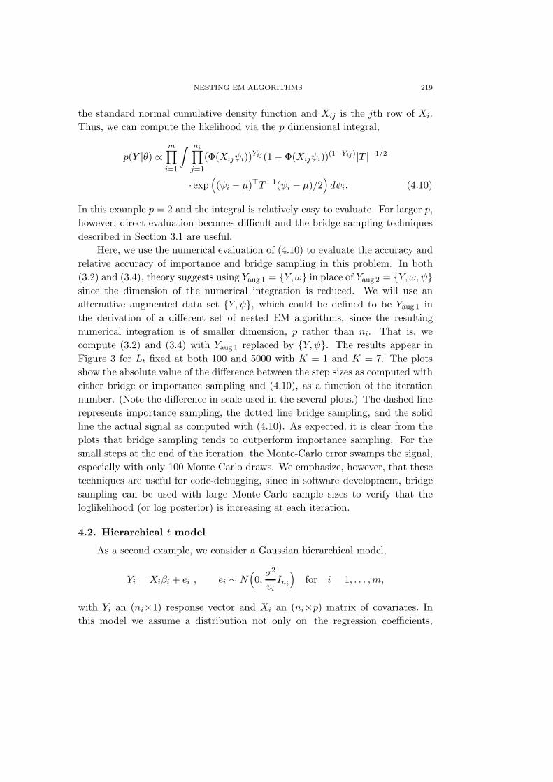
Here, we use the numerical evaluation of (4.10) to evaluate the accuracy andrelative accuracy of importance and bridge sampling in this problem. In both(3.2) and (3.4), theory suggests using Yaug 1 = {Y, ω} in place of Yaug 2 = {Y, ω, ψ}since the dimension of the numerical integration is reduced. We will use analternative augmented data set {Y, ψ}, which could be defined to be Yaug 1 inthe derivation of a different set of nested EM algorithms, since the resultingnumerical integration is of smaller dimension, p rather than ni. That is, wecompute (3.2) and (3.4) with Yaug 1 replaced by {Y, ψ}. The results appear inFigure 3 for Lt fixed at both 100 and 5000 with K = 1 and K = 7. The plotsshow the absolute value of the difference between the step sizes as computed witheither bridge or importance sampling and (4.10), as a function of the iterationnumber. (Note the difference in scale used in the several plots.) The dashed linerepresents importance sampling, the dotted line bridge sampling, and the solidline the actual signal as computed with (4.10). As expected, it is clear from theplots that bridge sampling tends to outperform importance sampling. For thesmall steps at the end of the iteration, the Monte-Carlo error swamps the signal,especially with only 100 Monte-Carlo draws. We emphasize, however, that thesetechniques are useful for code-debugging, since in software development, bridgesampling can be used with large Monte-Carlo sample sizes to verify that theloglikelihood (or log posterior) is increasing at each iteration.

4.2. Hierarchical t model

As a second example, we consider a Gaussian hierarchical model,

Yi = Xiβi + ei , ei ∼ N(0,σ2

viIni

)for i = 1, . . . ,m,

with Yi an (ni×1) response vector and Xi an (ni×p) matrix of covariates. Inthis model we assume a distribution not only on the regression coefficients,


0

0

00

5

55

1010

1010

15

1515

20

2020

25

2525

30

3030

0.0

0.0

0.0

0.4

0.8

0.0

50.1

50.2

5

0.0

10.0

20.0

30.0

4

5000 Monte-Carlo Draws


iterationiteration

iterationiteration

Monte

-Carl

oErr

or

Monte

-Carl

oErr

or

Monte

-Carl

oErr

or

Monte

-Carl

oErr

or



13

2

2

4 6 8

1.2

Figure 3. Approximating Step Sizes Using Importance and Bridge Sampling.The four plots compare importance sampling with bridge sampling for com-puting the step size in loglikelihood of each iteration. The actual step size ascomputed by numerical integration is given by the solid line, the other twolines record the difference between the solid line and what was reported byimportance sampling (dashed line) and bridge sampling (dotted line). Theplots in the left column correspond to 100 Monte-Carlo draws; those in theright column correspond to 5000 draws. The first row represents the EMalgorithm, the second the nested EM algorithm with K = 7. Notice that forthe early iterations (especially with a larger number of Monte-Carlo draws)both importance sampling and bridge sampling do a reasonable job relativeto the size of the signal given by the solid line. Bridge sampling, however,tends to out perform importance sampling. Since the nested algorithm takesbigger steps, the error in both importance and bridge sampling is larger thanwith the standard EM algorithm.

βi ∼ N(µ, T ) as in the common random-effects model, but also on the variances,through the latent variable, vi ∼ χ2

ν/ν, where ν is typically fixed and representsthe variability among the group variances. We refer to this model as a hierarchicalt-model since the conditional distribution of Yi given βi is multivariate t. In orderto derive an EM algorithm, we define Yaug = {(Yi, βi, vi), i = 1, . . . ,m}, but notethat Q(θ|θ(t)), with θ = (σ, µ, T ), cannot be evaluated in closed form and must beapproximated via Monte-Carlo integration. In particular, given θ we can run aGibbs sampler using the complete conditional distributions of the latent variableswhich are given by

βi|v, Y, θ ∼ Np(βi(Wi(vi)), T − TX�i Wi(vi)XiT ), i = 1, . . . ,m,


where Y = (Y1, . . . , Ym), v = (v1, . . . , vm),

βi(Wi(vi)) = µ+ TX�i Wi(vi)(Yi −Xiµ) with Wi(vi) =

[σ2

viIni +X�

i TXi

]−1

and

vi|β, Y, θ ∼ Gamma

(ν + 1

2,

12(ν + d2

i )

),

when β = (β1, . . . , βm) and d2i = (Yi − Xiβi)�(Yi − Xiβi)/σ2. (The Gamma

distribution is parameterized so that E [νi|β, Y, θ] = (ν + 1)/(ν + d2i ).) The M-

step maximizes Q(θ|θ(t)) by setting

µ(t+1) =1m

m∑i=1

E[βi|Y, θ(t)

], (4.11)

T (t+1) =1m

m∑i=1

(E[βiβ

�i |Y, θ(t)

]− E

[βi|Y, θ(t)

]E[βi|Y, θ(t)

]�), (4.12)

and

[σ2](t+1) =1n

m∑i=1

E[vi(Yi −Xiβi)�(Yi −Xiβi)|Y, θ(t)

]

=1n

m∑i=1

(E[vi|Y, θ(t)

]Y �

i Yi − 2Y �i XiE

[viβi|Y, θ(t)

](4.13)

+ tr(XiE

[viβiβ

�i |Y, θ(t)

]X�

i

)). (4.14)

The five different expectations in (4.11) and (4.14) are approximated using aMonte-Carlo E-step with the Gibbs sampler described above. Again we use Rao-Blackwellizied forms:

E[βi|Y, θ(t)

]= E

[βi(Wi(vi))|Y, θ(t)

]≈ βi(S1i) where S1i =

1Lt

Lt∑l=1

Wi(v(l)i ),

(4.15)with {v(1)

i , . . . , v(Lt)i } being the Lt draws of vi at iteration t (for i = 1, . . . ,m),

E[βiβ

�i |Y, θ(t)

]= E

[βi(Wi(vi))[βi(Wi(vi))]�|Y, θ(t)

]+ T − TX�

i S1iXiT, (4.16)

where E [βi(Wi(vi))[βi(Wi(vi))]�|Y, θ(t)]≈ βi(S1i)µ�+µ(βi(S1i)−µ)�+TX�i S2iXiT

with S2i given by 1Lt

∑Ltl=1Wi(v

(l)i )(Yi −Xiµ)(Yi −Xiµ)�Wi(v

(l)i ),

E [vi|Y, θ(t)] ≈ S3i where S3i =1Lt

Lt∑l=1

v(l)i , (4.17)


E [viβi|Y, θ(t)] = E[viβi(Wi(vi))|Y, θ(t)

]≈ µS3i + TX�

i S4i(Y −Xiµ), where

S4i =1Lt

Lt∑l=1

v(l)i Wi(v

(l)i ), (4.18)

and

E [viβiβ�i |Y, θ(t)]=E

[vi

(βi(Wi(vi))[βi(Wi(vi))]�+T − TX�

i Wi(vi)XiT)|Y, θ(t)

]≈S3iµµ

� + TX�i S4i(Y −Xiµ)µ�+

[TX�

i S4i(Y −Xiµ)µ�]�

+TX�i S5iXiT + S3iT − TX�

i S4iXiT, (4.19)

where S5i = 1Lt

∑Ltl=1 v

(l)i Wi(v

(l)i )(Yi −Xiµ)(Yi −Xiµ)�Wi(v

(l)i ). Thus, one itera-

tion of the EM algorithm first computes {Sji, j = 1, . . . , 5, i = 1, . . . ,m} using Lt

Monte-Carlo draws of v, then uses these statistics to compute the expectationsgiven in (4.15) – (4.19), and finally updates the parameters via (4.11) – (4.14).In the nested EM algorithm we set Yaug 1 = {Y, v} and Yaug 2 = {Y, v, β} sothat {(v(1)

i , . . . , v(Lt)i ), i = 1, . . . ,m} only needs to be drawn in the first cycle of

each iteration. In subsequent cycles, the E-step consists of reevaluating {Sji, j =1, 2, 4, 5, i = 1, . . . ,m} and (4.15) – (4.19) using the updated parameter values,and the M-step is given by (4.11) and (4.14). Because E (�(θ|Yaug 2)|Yaug 1, θ0)is not linear in v, the Monte-Carlo estimates Sji for j = 3 must be computedat each cycle of the algorithm. Despite this, nesting significantly reduces thecomputational requirement of the algorithm because the Gibbs sampler is onlyrun during the first cycle of each iteration.

In order to further increase computational efficiency, we introduce a work-ing parameter into the marginal distribution of vi. In particular, we replaceYaug 1 = {Y, β, v} with Yaug 1 = {Y, β, u}, where ui = αvi for i = 1, . . . ,m. Com-putationally, the effect of this change is simply that (4.13) – (4.14) is replacedby

[σ2](t+1) =1∑m

i=1 niS3i

m∑i=1

(E[vi|Y, θ(t)

]Y �

i Yi − 2Y �i XiE

[viβi|Y, θ(t)

]

+ tr(XiE[viβiβ

�i |Y, θ(t)

]X�

i )).

That is, the division by n is replaced by division by the “sum of the weights”.See Meng and van Dyk (1997) for discussion of this substitution in the non-hierarchical t-model.

Figure 4 illustrates the relative computational cost of the EM and the nestedEM algorithms using K = 3, 5, 7, and 15. The hierarchical t model with ν =10 was fit to data from an orthodontic study (Potthoff and Roy (1964)). The


distance between the pteryomaxillary fissure and the center of the pituitary wasmeasured on 16 boys at age 8, 10, 12, and 14. Here Yi are the four measurementsfor boy i, and the covariates consist of an intercept term and age. In Figure 4,Lt was set to 20t. Although there is some variability as a function of K in theamount of improvement, nesting reduces the computation time by a factor ofbetween three (when K is small) and ten (when K is large).

•••••••••

••••••

••• • • • • • • • • • • • • • • • • • • • • • • • • • • • • • • • •

••••••

••••

•••••••••

•••••••••• • • • • • • • • • • • • • • • • • • •

seconds

seconds

loglikelihood

loglikelihood

loglikelihood

0

0

0

10

50

advanta

ge

ofnest

ing

24

68

12

100 150

200

200

-100

-100

-95

-95

-90

-90

-85

-85

-80

-80

400 600 800 1000

-76.5

0-7

6.4

8-7

6.4

6-7

6.4

4

Figure 4. Fitting a Hierarchical t-Model Increasing the Number of Monte-Carlo Draws by 20 at Each Iteration. The components of this figure areidentical to those of Figure 1. Again we increase the number of draws ateach iteration to stabilize the convergence of the algorithms. The nestedalgorithms, espescially with large K, show substantial improvement over thestandard algorithm.

5. Discussion

The EM algorithm is a useful tool for computing maximum likelihood esti-mates and posterior modes for models involving latent variables or missing data.Even when MCMC methods are used to map out the posterior or likelihood


more completely, the location of the (multiple) modes is invaluable for determin-ing starting vales and the EM computer code typically forms the backbone ofthe computer code for the Gibbs sampler (so programming effort is kept to aminimum). In models formulated in terms of multiple latent variables, standardoptimization techniques such as Newton-Raphson type algorithms not only suf-fer from stability problems when �(θ|Y ) is far from quadratic, but also can bedifficult to implement when numerical integration is required to evaluate �(θ|Y ).In these settings the (Monte-Carlo) EM algorithm offers a stable albeit slow so-lution, requiring little programming that is not required by the Gibbs sampleritself. By nesting we can both maintain the stability of EM and increase thecomputational efficiency while requiring essentially no extra effort by those whoimplement the algorithm.

Acknowledgements

The research was supported in part by the NSF grant DMS 97-05156 andby the U.S. Census Bureau. The author thanks an anonymous referee for manyhelpful comments.

References

Chan, J. S. K. and Kuk, A. Y. C. (1997). Maximum likelihood estimation for probit-linearmixed models with correlated random effects. Biometrics 53, 86-97.

Chan, K. S. and Ledolter, J. (1995). Monte Carlo EM estimation for time series models involvingcounts. J. Amer. Statist. Assoc. 90, 242-252.

Dempster, A. P., Laird, N. M. and Rubin, D. B. (1977). Maximum likelihood estimation fromincomplete-data via the EM algorithm (with discussion). J. Roy. Statist. Soc. Ser. B 39,

1-38.Fessler, J. A. and Hero, A. O. (1994). Space-alternating generalized expectation-maximization

algorithm. IEEE Tran. on Signal Processing 42, 2664-2677.

Levine, R. A. and Casella, G. (1999). Implementations to the Monte Carlo EM algorithm.Submitted to J. Comput. Graphical Statist.

Liu, C., Rubin, D. B. and Wu, Y. N. (1998). Parameter expansion for EM acceleration: thePX-EM algorithm. Biometrika 85, 755-770.

Liu, J. S., Wong, W. H. and Kong, A. (1995). Covariance structure and convergence rate of theGibbs sampler with various scans. J. Roy. Statist. Soc. Ser. B 57, 157-169.

McCulloch, C. E. (1994). Maximum likelihood variance components estimation for binary data.J. Amer. Statist. Assoc. 89, 330-335.

McCulloch, C. E. (1997). Maximum likelihood algorithms for generalized linear mixed models.

J. Amer. Statist. Assoc. 92, 162-170.McLachlan, G. J. and Krishnan, T. (1997). The EM Algorithm and Extensions. John Wiley &

Sons, New York.Meng, X. L. and Schilling, S. (1996). Fitting full-information item factor models and an empir-

ical investigation of bridge sampling. J. Amer. Statist. Assoc. 91, 1254-1267.Meng, X. L. and Rubin, D. B. (1994). On the global and componentwise rates of convergence

of the EM algorithm. Linear Algebra and Its Applications (Special issue honoring Ingram

Olkin) 199, 413-425.


Meng, X. L. and van Dyk, D. A. (1997). The EM algorithm – an old folk song sung to a fast

new tune (with discussion). J. Roy. Statist. Soc. Ser. B 59, 511-567.

Meng, X. L. and van Dyk, D. A. (1998). Fast EM implementations for mixed-effects models.

J. Roy. Statist. Soc. Ser. B 60, 559-578.

Meng, X. L. and van Dyk, D. A. (1999). Seeking efficient data augmentation schemes via

conditional and marginal augmentation. Biometrika 86, 301-320.

Meng, X. L. and Wong, W. H. (1996). Simulating ratios of normalizing constants via a simple

identity: a theoretical exploration. Statist. Sinica 6, 831-860.

Potthoff, R. F. and Roy, S. N. (1964). A generalized multivariate analysis of variance model

useful especially for growth curve problems. Biometrika 51, 313-326.

Roberts, G. O. and Sahu, S. K. (1997). Updating schemes, correlation structure, blocking and

parameterization for the Gibbs sampler. J. Roy. Statist. Soc. Ser. B. 59, 291-317.

van Dyk, D. A. (1998). Nesting EM algorithms for computational efficiency. Unpublished

Technical Report.

van Dyk, D. A. (2000a). Fitting mixed-effects models using efficient EM-type algorithms. J.

Comput. Graphical Statist. To appear.

van Dyk, D. A. (2000b). Fast new EM-type algorithms with applications in astrophysics.

Submitted to The Astrophysical J.

van Dyk, D. A., Conners, A., Kashyap, V. and Siemiginowska, A. (2000). Analysis of energy

spectra with low photor counts via Bayesian posterior simulation. Unpublished Technical

Report.

van Dyk, D. A. and Meng, X. L. (1999). The art of data augmentation. Submitted to Ann.

Statist.

Wei, G. C. G. and Tanner, M. A. (1990). A Monte Carlo implementation of the EM algorithm

and the poor man’s data augmentation algorithm. J. Amer. Statist. Assoc. 85, 699-704.

Wu, C. F. J. (1983). On the convergence properties of the EM algorithm. Ann. Statist. 11,

95-103.

Department of Statistics, Harvard University, Science Center, One Oxford Street, Cambridge,

MA 02138, U.S.A.

E-mail: [email protected]

(Received April 1998; accepted March 1999)

nesting em algorithms for computational efficiencydvandyk/research/00-sinica-nem.pdf · statistica...

Documents