Presentation Identifier (Title or Location), Month 00, 2008

New Developments in Combustion

Technology Part III: Making oxy-fuel combustion an advantage

Geo. A. Richards, Ph.D.

National Energy Technology Laboratory - U. S. Department of

Energy

2014 Princeton-CEFRC Summer School On Combustion

Course Length: 6 hrs

June 22-23, 2014

‹#›

This presentation

Updated, expanded from 2012 CEFRC lecture:

– Inherent carbon capture: chemical looping combustion (Day 1)

– Step-change in generator efficiency: pressure gain combustion (Day 2)

– Frontier approach (?!): making oxy-fuel an efficiency advantage (Day 2)

P-gain rig @ NETL

RDC

Sampling

&

Diagnostics

Flow

‹#›

Making oxygen for oxy-fuel …reprise • Oxygen can be supplied today by commercial Air Separation Units

(ASU) based on established cryogenic separation.

• The energy needed to separate oxygen from air is significant (see

below)

• In conventional oxy-combustion, we dilute the purified oxygen to

maintain the same boiler flame temperature as in air-combustion.

Air

Separation

Unity

(ASU)

1 mole of air

0.21 moles oxygen

pO2 = 0.21 atm

0.79 moles nitrogen

pN2 = 0.79 atm

0.21 moles oxygen

pO2 = 1 atm

0.79 moles nitrogen

pN2 = 1 atm

Reversible separation work:

~6 kJ/gmol O2 produced*

Current actual process:

~18kJ/gmol O2 produced**

*e.g, the change in gibbs energy for ideal mixing (Sandler, Chemical Engineering Thermodynamics (1989) pp. 313.

**See Trainier et al., “Air Separation Unit…..” Clearwater Coal Conference, 2010.

C + O2 CO2

DH ~ DG = 394 kJ/gmol (C or O2)

In efficient powerplants we convert

less than ½ of DH to work.

Thus~200kJ/gmol O2 work produced

Roughly ~1/10 of that is needed for ASU.

Dilute again

with CO2 or steam

‹#›

Making Oxy-fuel an Advantage • Producing pure oxygen requires a lot of energy!

• If one could find a way to make significant extra power because of the

available oxygen, oxy-fuel would be an advantage.

• Oxy-fuel already provides an advantage for process industries that

benefit from high temperatures (e.g., glass making, steel).

• Oxy-fuel already provides advantages in propulsion (rocket engines)

• How can you make oxy-fuel an advantage for power generation?

‹#›

Efficiency

A) Existing Supercritical Pulverized

Coal (23.9MPa/866K/866K steam)1

B) Advanced Ultra-Supercritical

Pulverized Coal (34.5 Mpa/1005K/1033K

steam)1

C) Simple Cycle Gas Turbine (as

reported, LMS 100, working fluid temp

estimated from exhaust and pressure ratio)2

D) Combined Cycle Gas Turbine (as

reported, MPCP2(M501J), working fluid temp

estimated similar to case C)3

0

10

20

30

40

50

60

70

80

90

100

0 500 1000 1500 2000 2500

Temperature (K)

A B

D

C

Eff

icie

ncy

[1] Current and Future Technologies for Power Generation with Post-Combustion Carbon Capture, DOE/NETL-2012/1557

[2] Gas Turbine World 2012 GTW Handbook, Vol. 29, Pequot Publishing pp74

[3] Gas Turbine World 2012 GTW Handbook, Vol. 29, Pequot Publishing pp89

Gas Turbine Combustion Temp. = Working fluid temp.

PC Coal Combustion Temp. >> Working fluid temp.

Oxy-fuel Combustion Temp. >> >>Working fluid temp.

Carnot w/r to 293 K

Note: boilers report HHV efficiency;

turbines report LHV

Approximate combustion temperatures

‹#›

Magnetohydrodynamic Power Generation

• The high temperatures

possible with oxy-fuel can be

used to operate an MHD

“topping” cycle:

– Topping cycle power possible

because of the oxygen

– MHD exits to conventional

steam boiler system

(“bottoming cycle”).

• How does MHD work?

– Conductive, high-temperature

gases play the role of an

electrical conductor moving

through a magnetic field.

– Generates power directly from

the moving gases.

- +

A Turbogenerator

B MHD Generator

Hot Vapor

or Gas

Moving

Conductors

Forming Coil

Brushes

Motion

of Gas

Field

External

Current

Electrode

Cathode

Electromotive

Force

Source of Hot,

Electrically

Conducting Gas

N

S

N

S

‹#›

A combined cycle • For reasons that will be clear later, most MHD concepts only

produce power ABOVE ~ 2600K (which is….HOT!).

• Thus, it needs to be a combined cycle to extract energy from

the whole temperature spectrum.

MHD Power Unit

~ 45% efficient today best cases MHD “topping” cycle including the oxygen production

Fuel

Oxygen

2600 K

combustion

products

High efficiency

steam boiler

Air

separation

unit Air

Topping Work Output WT Bottoming Work Output WB

Enthalpy into the “top” = mass flow of fuel x HHV = Q

Work from the top : WT = hT Q

Enthalpy into the “bottom” = Q – WT = Q ( 1 – hT ) Work from the bottom: WB = hB (Enthalpy into the bottom) = Q ( hB – hT hB )

Combined cycle efficiency: (WT + WB)/Q = hT + hB – hT hB

Example

hT = 0.1 (10%)

hB = 0.45 (45%)

Combined

Efficiency:

.1+.45 – (.1)(.45)

= 0.50 (50%)

‹#›

Past MHD topping efforts

• Concept proven in

both U.S. and USSR

in 70s and 80s

– US DOE 1978-

1993

– Electricity

transferred to grid

• Economic downfall :

key factor being

materials

– Electrode damage

– Seed material use

MHD U25RM diffuser channel (USSR) 1970s

From Petrick & Shumyatsky 1978.

‹#›

Direct Power Extraction The “new” MHD: making oxy-fuel an advantage

New benefits, new approaches, new technology:

Legacy MHD program Today Comments

No CO2 capture CO2 Capture Oxy-fuel combustion developed for

capture enables MHD.

Large demos Simulation & validation Validated models for different

generator concepts, not demos.

Pre-heated air Efficient oxygen production ASU power requirements have

dropped 40% since 1990.

SOx and NOx control Capture GPU No emissions! Use oxy-fuel gas

processing unit (GPU).

Magnets < 6 Tesla Magnets > 6 Tesla Advanced magnets exist today.

Analog electronics Solid-state inverters/control Electrode arcing could be controlled

with digital devices.

Linear generator Radial, Linear, others Simulations can compare multiple

geometries.

Conventional manufacturing Advanced manufacturing New channel construction

approaches.

Seeded flows New goal: injected plasma Aspirational – use nanosecond

pulse discharge to ionize gas ?

‹#›

Related technology – combustion, ionized flames, and plasma

• Non-equilibrium plasma may benefit new aspects of combustion: Starikovsky, A. Aleksandrov, N. (2013). Plasma-Assisted Ignition and Combustion, Progress in Energy and Combustion Science, Vol. 39, pp. 61-110.

Ignition in demanding applications - Pulse detonation engines, gas turbine re-light, HCCI engines, others

• Alternating current excitation of flames has recently demonstrated significant

hydrodynamic changes in flame structures: Drews, A. M., Cademartiri, L., Chemama, M. L., Brenner, M. P., Whitesides, G. M., Bishop, K. J. M (2012).

AC Electric Fields Drive Steady Flows in Flames, Physical Review E 86, pages 036314-1 to 4.

“…AC fields induce steady electric winds….localized near the surface of the flame….these results suggest that ac fields can

be used to manipulate and control combustion processes at a distance….”

• Flame ionization can be used for sensors and diagnostics. Benson, K., Thornton, J. D., Straub, D. L., Huckaby, E. D., Richards, G. A. (2005). Flame Ionization Sensor Integrated Into a Gas Turbine Fuel Nozzle,

ASME J. Eng. Gas Turbines and Power, Vol. 127, No. 1, pp. 42-48.

Proposes detection of dynamics and combustion conditions with flame ionization

• New propulsion concepts include plasma - MHD “bypass” or electric thrust propulsion: Schneider, S. (2011). Annular MHD Physics for Turbojet Energy Bypass, AIAA-2011-2230.

Longmeier, B. W., Cassady, L. D., Ballenger, M. G., McCaskill, G. E., Chang-Diaz, F. R., Bering, E. A. (2014). Improved Efficiency and Throttling

Range of the VX-200 Magnetoplasma Thruster, Journal of Propulsion and Power, Vol. 30, No. 1 pp. 123 – 132.

• Non-equilibrium plasma: a key technology for the future? Plasma Science: Advancing Knowledge in the National Interest (2010). http://www.nap.edu/catalog/11960.html

This National Academies report provides status and motivation to use plasma – including combustion applications.

Inlet

MHD enthalpy

extraction MHD accelerator

Turbo-jet

Mach 7

Plasma television

display

http://en.wikipedia.org/wi

ki/Plasma_display

MHD Bypass Concept

‹#›

Fundamentals of Electromagnetics

• Electric field E is a vector (units: volt/meter)

• E can be described by the voltage potential V; E = - V*

• By convention, minus sign means E points to low voltage

• Magnetic Induction B is a vector (units: Tesla = voltsec/m2)

* Thus in 1-D E = -V/L

L = distance.

Experimental observations

of charge Q in electric

Field E (left) and moving

at velocity uQ in B (right).

ENET = E + uQ x B

Charge Q uQ

FB

B

FE

E

FE = Q E

Electric Force on Q

E = FE /Q

FB = Q (uQ x B)

Magnetic Force on Q

uQ x B = FB /Q

“Another” E !

‹#›

A Simple Generator

• Gas (conductive) flows with bulk velocity u i

• Magnetic filed B k is applied as shown.

• The resulting “induced” electric field is –uB k

• This field can drive a current flow in the external circuit.

• How is this similar to a conventional generator?

u x B = -uB k

Flowing

conductive

gases

RL B u b

k i

j

‹#›

How Much Current Flows? The current flux is proportioned to ENET:

I = = ;

RL

b CHANNEL

HEIGHT

SIMPLE GENERATOR FROM PREVIOUS PAGE

i

j

I

Define open circuit RL infinite, then J = 0 implies E0 = uB from above.

Then, VOC = uBb (open circuit voltage)

E0

uB

J

J = σ ENET ; σ = conductivity of media [Amps/(voltmeter)]

J = current flux vector [ Amps/meter2] A = electrode area [meter2]

J = σ ENET = σ ( E0 + u x B) = σ ( E0 – uB) j

From E0 = - V E0 = - (VL – VH ) /b

(VL = Low Voltage VH = High Voltage)

E0 = (VH – VL) /b = IRL/b (Ohm’s Law)

uBb

b/ σ A + RL

VOC

Ri+ RL

Ri ≡ internal resistance

VH

VL

Ri

Ri = b/sA is the resistance to current flow through

the plasma – shown “oddly” disconnected since

uB drives current in the same place.

Note : as typical, Voc is a voltage difference while VH and VL are measured relative to ground

Important

Nomenclature Note:

E0 (zero sub) is

applied by the external

load & does not

include magnetic

induced field

‹#›

Limiting Cases

RL = O E0 = 0

VH = VL

VH = VL

uB

VL

VH

E0

uB

O = J = σ ( E0 – uB) E0= uB

(VH – VL)/b = E0 = uB

VOC ≡ uBb

Open Circuit

E0 = (VH – VL)/b = O

I = =

Short Circuit

VOC

Ri+ RL=O

VOC

Ri

VL

VH

E0

uB

E0< uB; J = σ ( E0 – uB)

I = Voc/(Ri+RL)

Generating Circuit

RL Ri

Ri

J

J

‹#›

Electrical Analogy

Several interpretations for K:

1. Ratio of load to O.C. voltage

2. Ratio of load resistance to total resistance

3. An efficiency (why ? Multiply by I/I load power/total power)

4. A ratio of the “applied” field E0 to “generated” field uB

Define K = = = = VOC

VLoad

I (Ri + RL)

IRL

RL + Ri

RL

uB

E0

G

Ri

RL VOC = uBb

I

VLoad = E0b

‹#›

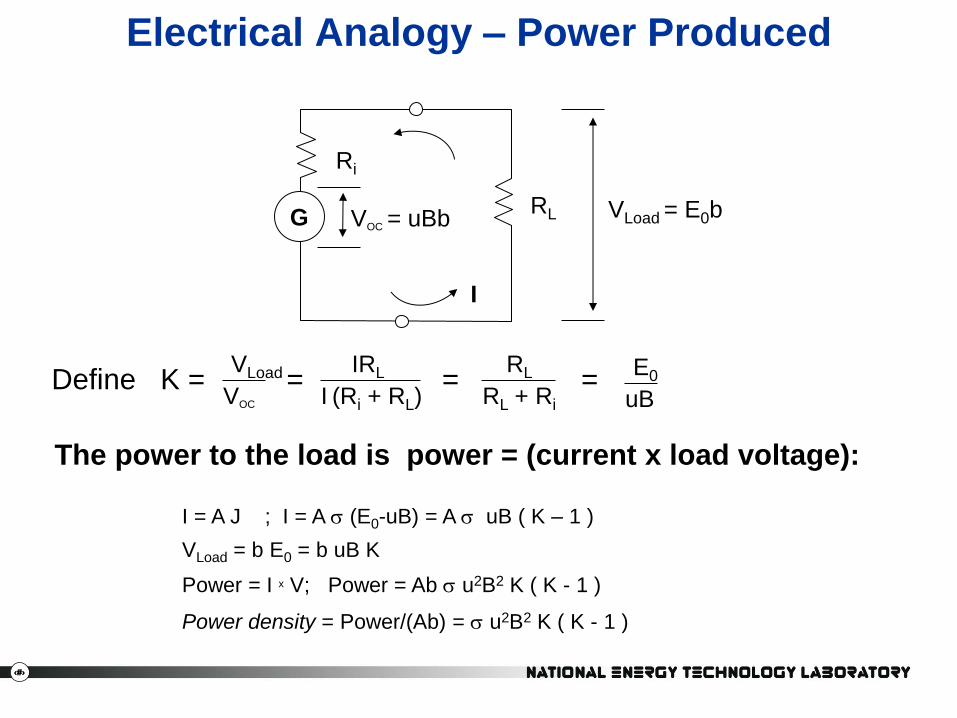
Electrical Analogy – Power Produced

The power to the load is power = (current x load voltage):

Define K = = = = VOC

VLoad

I (Ri + RL)

IRL

RL + Ri

RL

uB

E0

G

Ri

RL VOC = uBb

I

VLoad = E0b

I = A J ; I = A s (E0-uB) = A s uB ( K – 1 )

VLoad = b E0 = b uB K

Power = I x V; Power = Ab s u2B2 K ( K - 1 )

Power density = Power/(Ab) = s u2B2 K ( K - 1 )

‹#›

Next slides - overview

What you just heard:

Jy = σ (E0 – uB) a simple generator

What you will hear next:

• A complication arises from the Hall Effect

…the flowing current also interacts significantly with B

• Thus, we find:

• You can impose E0x or E0y by applying different electrical

boundary conditions via electrode geometry

Jx = (E0x - e B {E0y-uB}) I + eB

2

σ

Jy = ({E0y –uB}+ e B E0x) I + eB2

σ

‹#›

Complications From the Hall Effect

Hall Effect “Tilts” the Field – How Much? Caution: note this is a simplification for clarity; ue may not be aligned with the y-axis

• Most MHD: charge is carried by electrons

• By convention, electrons move against E

• The electron current flow has an associate charge velocity ue

• Must account for the interaction between ue and B (Hall Effect)

k

j

i

+ + + - - - u

u B

u x B

No Current :

charge velocity =

bulk velocity u

+ +

+ - - - u

u B electrons

electrons

u x B

ue x B Hall Effect

ue

‹#›

• The velocity of electrons in a field is ue = -e (Enet+ ue x B ) (i)

• The mobility e is related to conductivity as neee = σ

• The B field is assumed independent of current flow B = B k

• Notice that Jx = -nee uex ; Jy = -nee uey

ue = -e (Enet,xi + Enet,y j + ue x B)

Some Cyphering

B

Enet,y

Enet,x

Jx = (Enet,x – eB Enet,y) I + e2

B2

σ

Jy = (Enet,y + e B Enet,x) I + e2

B2

σ

ue = uex i + uey j Also assume

J = Jx i + Jy j

ne = electron # density (per m3)

e = fundamental charge 1.602 E-19 C/electron

e = electron mobility /

Nomenclature

m s

V m Enet,x = E0x

Enet,y = E0y – u B

Straightforward

algebra and

substitutions in

equation (i).

‹#›

Notice that the simple generator analysis (without Hall Effect) gave

Thus, the Hall Effect reduces the y- current by:

The Hall effect leads to an x-current that is e B times the y-current.

How big is e B? (Next Slide)

The Simple Faraday Generator y

x • The electrodes are long, continuous

• Thus, E0x = 0

u Jy = (Ey,net) = (E0y-uB)

I + e2

B2

σ

I + e2

B2

σ

k

j

i z

What is the magnitude of meaning of Jx?

Jx = (0- e BEnet,y) = (-e B [E0y-uB]) = -e B Jy I + e

2B2

σ

I + e 2B2

σ

(Jy) = σ (E0y-uB)

I + e2

B2

1

No Hall

‹#›

The Magnitude of eB

E = - Ex i

Consider the x-direction force on the electron between collisions time

Fe = me ; -eEx me ( )

But, we also write:

- eEx = ue, mean

x

dt due

ue, mean

Combining (i) and (ii) : e = e/me

We can also express a magnetic field in terms of a “cyclotron frequency” , next:

(ii)

(i)

(iii)

B

y

x

FB

ue

In the absence of other forces/collisions, the electron will experience a force

at right angles to its motion circular orbit rL, consider the force:

FB = -e(ue x B)

e B =

FB = - meue2

/ rL

-eueB = -meue2

/ rL = B r L

ue

e

me

(iv)

Define cyclotron frequency

= ue / rL B = me/e

Combine (iii) and (iv) :

>> 1 lots of cycles before collisions

~ 1 collide ~ one cycle

<< 1 lots of collisions before a cycle is complete

rL

“Hall parameter”

‹#›

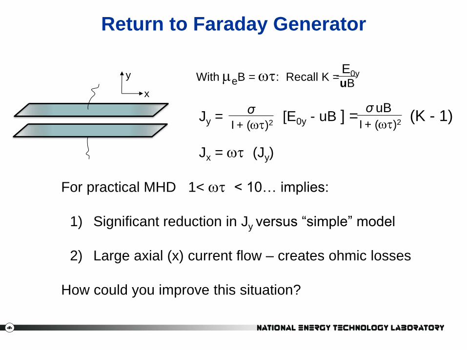
Return to Faraday Generator

y

x

Jy = [E0y - uB ] = (K - 1) I + ()2

Jx = (Jy)

σ

With eB = : Recall K =

For practical MHD 1< < 10… implies:

1) Significant reduction in Jy versus “simple” model

2) Large axial (x) current flow – creates ohmic losses

How could you improve this situation?

uB

E0y

I + ()2

σ uB

‹#›

Segmented Electrodes Break up the x-current so that Jx = 0:

(why does this stop the Hall current?)*

u

Jx = (Ex,net - Ey,net) = 0 I + 22

σ

Jy = (Ey,net + Ex,net) I + 22

σ

(1)

(2)

From (1): Ex,net = Ey,net

(3)

y

x z (out of plane) Jy = (Ey,net + 22 Ey,net) = (1+22)

I + 22

σ

I + 22

σ Ey,net

Individual loads

Jy = σ Enet,y = σ (Eo - uB) Same as “simple” generator

Notice that the axial voltage gradient is potentially very large (eqn. 3)

* It has no return path.

What practical disadvantages exist with this concept?

‹#›

Hall Generators Here, you use the axial hall current for power. Notice Eyo = 0 by short circuit.

short circuit

(applied) Ey,net = Eyo - uB

Solve for currents and

voltage as before.

Eoc = - uB open circuit

LOAD

State one huge practical advantage of the disk? (Hint: count the number of wires)

Notice the open circuit voltage is larger than uB

KH = (Defined) Disk Geometry (very clever!)

-Eox uB

+ u

LOAD

B Hall current

u x B current

(short circuit)

Flow out

Flow in

‹#›

An intermediate approach:

Slanted (diagonal) electrode connections

• Electrode connections establish E0x and E0y so that the

electrons experience a force from the Hall field that is

balanced by the E0x imposed by the electrodes.

• Thus, the current only flows vertically in the channel.

• This balance exists at just one operating condition.

From: Quarterly Technical Progress Report, July 1 – Sept 30, 1985, Component Development and Integration Facility

Work performed under DOE DE-AC07-781D01745; Original Reports currently available only at NETL .

Note the slanted electrode frames visible in the duct Force from

(E0y-uB) Force from

Hall effect

Force from

x-electric field Avg. drag

force from

collisions

See Hill and Peterson

“Mechanics and

Thermodynamics of

Propulsion” Third Printing,

1970, Addison-Wesley

Publishing, pp. 122. Helpful

discussion of the force

balance. Electron

velocity

Load

Load

E0

E0x

E0y

Note that the Enet includes –uB in the y-direction.

The electrons move vertically in response to (E0y-uB)

B points out of the page

u

‹#›

Fluid mechanics and thermodynamics

Ohmic loss:

per unit

volume:

G

R

Current: I = J A

Voltage: V = E0 b Height

b

Area A

Volume: V = b A Resistance:

R= b/(As)

Flow Velocity

u

per unit

volume:

Electrical power output from the volume:

Note: in a 2 or 3D problem the output is the dot product of vectors - J . E0 . Care must be used on the sign of scalars in simple balance laws, and distinguishing output (MHD generator) versus input (MHD pump)

E0

Use the earlier definition of load factor K; recall 0 < K < 1, use (i – iii)

Mechanical energy input to the volume (x-body force times x-velocity u):

x-body force per unit volume: Force on a charge Q = (-e)

Charges per unit volume

Note u has only x-component;

Thus, mechanical energy input per unit volume:

(i)

(iii)

(ii)

Treating J as a negative scalar (current flowing down):

As expected : (1) + (2) = (3)

B

1-D Energy Balance

;

The vector product points left

‹#›

A summary of mass, momentum and energy (1-D simplification, steady flow, constant area duct, neglect thermal conduction and viscous effects)

For a comprehensive development of the governing equations, see for example: Hughes W.F., Young, F. J. (1989). The

Electrodynamics of Fluids, 2nd Edition, Robert E. Krieger Publishing.

Again, treat J as a negative scalar

Continuity: Familiar

Momentum eqn: Note JB is the body force from last page.

With negative J, what does this do to pressure along X?

Energy eqn: note this is written with the source

term (right side) as the negative of the output

defined on the last page. What does the source

term do to the enthalpy of the flow along X? = - (output)

U J

Electrodes

The real situation:

Describe the flow near the electrodes?

‹#›

Conductivity in the gaseous media

• In conventional electrical generators, a long copper

wire moves at a relatively slow speed through a

modest magnetic field.

• The conductivity of the gases in MHD is

comparatively low, even when “seeded”, next slide.

• MHD power extraction is practical only because of

the high velocity U, strong field B, large volume

conductor, and “adequate” conductivity

Power output density = -J • E0 = -σ U2B2K (K-1)

Copper s ~ = 6 x 107 Siemen/m

Seeded MHD s ~ = 10 Siemen/m Siemen = 1/ohm

‹#›

Gas Conductivity: Seeding Current flow depends on

conductivity J = σ E

Simple generator: Power density

P = -J • E0 = -σ U2B2K (K-1)

The power density is maximum at

K = ½ ∴ Pmax = σ U2B2/4

Reasonable Design:

10MW/m3 = Pmax; UB = 2000V/M

σ ≈ 10 S/m (S=Siemen = 1/ohm)

Two points: 1. The magnitude of the conductivity with

temperature: operating temp ~ > 2600K

2. The slope versus temperature: very sensitive

Species

Li

Na

K

Cs

He

Ne

A

H2

O2

O

N2

NO

CO

CO2

H2O

OH

U

Ionization

potential

Ei (eV)

5.39

5.14

4.34

3.89

24.58

21.56

15.76

15.6

12.05

13.61

15.6

9.26

14.1

14.4

12.6

13.8

6.1

Ionization Potentials Data from Swithenbank, J, (1974),

Magnetohydrodynamics and Electrodynamics of

Combustion Systems, in “Combustion Technology: Some

Modern Developments” Palmer, H.B., Beer, J.M. [eds]

Academic Press. Conductivity is for JP4-oxygen

combustion products with 1% K seed.

1

10

100

1500 2500 3500

Co

nd

cu

tivit

y (

S/m

)

Temperature (K)

J

Electrodes

The real situation:

Describe the conductivity near the electrodes?

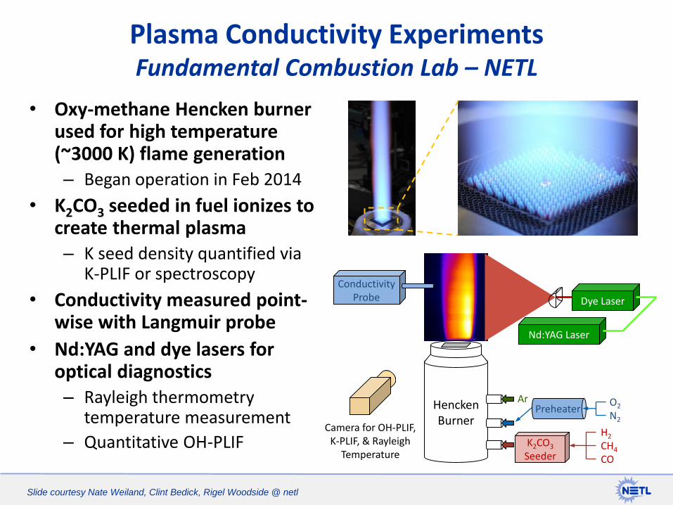
• Oxy-methane Hencken burner used for high temperature (~3000 K) flame generation – Began operation in Feb 2014

• K2CO3 seeded in fuel ionizes to create thermal plasma – K seed density quantified via

K-PLIF or spectroscopy

• Conductivity measured point-wise with Langmuir probe

• Nd:YAG and dye lasers for optical diagnostics – Rayleigh thermometry

temperature measurement

– Quantitative OH-PLIF

Plasma Conductivity Experiments Fundamental Combustion Lab – NETL

Hencken Burner

K2CO3

Seeder

H2

CH4

CO

Ar Preheater

O2

N2

Nd:YAG Laser

Dye Laser

Camera for OH-PLIF, K-PLIF, & Rayleigh

Temperature

Conductivity Probe

Slide courtesy Nate Weiland, Clint Bedick, Rigel Woodside @ netl

• Elements K and e (Electron) added • Species K, K+, KO, KOH, OH-, and Electron added • K/O/H reaction data added from: P. Glarborg, P. Marshall, “Mechanism

and modeling of the formation of gasous alkali sulfates”, Combustion and Flame 141, 22-39 (2005)

K + O + M <=> KO + M K + OH + M <=> KOH + M K + HO2 <=> KOH + O K + HO2 <=> KO + OH K + H2O2 <=> KOH + OH K + H2O2 <=> KO + H2O KO + H <=> K + OH KO + O <=> K + O2 KO + OH <=> KOH + O KO + HO2 <=> KOH + O2 KO + H2 <=> KOH + H KO + H2 <=> K + H2O KO + H2O <=> KOH + OH KO + CO <=> K + CO2 KOH + H <=> K + H2O • Ionization reaction data added from: D.E. Jensen, G.A. Jones, “Reaction

rate coefficients for flame calculations”, Combustion and Flame 32, 1-34 (1978)

K+ + Electron + M <=> K + M (factor of uncertainty = 5) OH + Electron + M <=> OH- + M (factor of uncertainty = 100)

Reaction Mechanism

Slide courtesy Nate Weiland, Clint Bedick, Rigel Woodside @ netl

• Steady state simulation composition matches CEA equilibrium fairly well; Cantera case is burner stabilized flame, noting T< Tad :

– CEA: 3022 K

– Cantera: 2815 K (burner stabilized heat loss)

• Major species reach equilibrium in <1 mm

1-D Flame Modeling in Cantera

0

0.05

0.1

0.15

0.2

0.25

0.3

0.35

0.4

0.45

O2 H2O CO2 CO OH O H

Spec

ies

Mo

le F

ract

ion

CEA Equilibrium

Cantera Steady State

0.00001

0.0001

0.001

0.01

K KO KOH K+ OH- e-

Spec

ies

Mo

le F

ract

ion

CEA Equilibrium

Cantera Steady State

0

0.1

0.2

0.3

0.4

0.5

0.6

0 0.2 0.4 0.6 0.8 1

Spec

ies

Mas

s Fr

acti

on

Axial Position (mm)

CH4 O2 H2O

CO2 CO OH

Slide courtesy Nate Weiland, Clint Bedick, Rigel Woodside @ netl

Conductivity & Seed Density Measurements

• Conductivity Measurements – Using a commercial Langmuir Double

Probe from Impedans, Ltd.

– Custom shaped platinum probe tips to achieve 1 mm2 resolution in flame

– Shape of induced current profile vs. probe voltage differential used to obtain electrical conductivity, electron temperature, and ion density (Osaka, 2008; Wild, 2012)

• K-PLIF Imaging – Need quantitative measure of seed

density for correlation to plasma conductivity

– K-PLIF used by Lengel & Linder (1990)

– Use K-atom transition at 578.2 nm (Monts, 1995) with existing laser dye

Nd:YAG Laser

Intensified

Camera

Cyl.

Lens Sph.

Lens

Hencken

Burner

2ω Gen 532 nm

70 mJ

Dye

Laser

578.2 nm

1 mJ Cyl.

Lens

Power

Monitor

Custom platinum

probe tips

Probe Potential (V)

Pro

be C

urr

en

t (μ

A)

Slide courtesy Nate Weiland, Clint Bedick, Rigel Woodside @ netl

‹#›

Seeding – not the same today? • Seeding is used to raise the conductivity of the

combustion products.

• The seed recovery was a major cost item and

technical barrier in earlier MHD programs.

• Would this change in a carbon capture scenario

where the entire flue gas was sought for capture?

• Non-equilibrium plasma generated would be a game

changer if :

– Energy to generate was low enough.

– Recombination rate was low.

– Studies for propulsion applications, using nano-

second discharge pulses: about 2 order of magnitude

greater ionization needed (?)*

* Schneider, S. (2011). Annular MHD Physics for Turboject Energy Bypass”, AIAA-2011-2230

‹#›

Electrodes • Cooled electrodes must operate with high surface temperature to

reduce quenching conductivity and heat loss near the walls.

• Complicated by thermal, chemical, and electrical attack.

• Some tests suggest reasonable life is possible in slag free (gas fuel

operation) or with better slag removal.

• Advances in materials and material processing for conductive solid

oxides – Field Assisted Sintering Technology- currently under

investigation at NETL.

• Current instability can lead to arcing – concentrated current flows –

burning the surface.

– State of the art electronics may reduce this problem

Cooled electrode from legacy test program,

Damage from arcing evident.

S. Chanthapan, A. Rape, S. Gephart, Anil K. Kulkarni, J. Singh (2011).

Industrial Scale Field Assisted Sintering Is an Emerging Disruptive

Manufacturing Technology ADVANCED MATERIALS & PROCESSES, pp.

21-26, Published by ASM.

Compress

Pulse DC Voltage Sintered material

can include

conductive

ceramics with

unique properties

‹#›

Layout of a Power Plant Configuration

What would be different

in a carbon capture

scheme?

What might be removed

for future electric grids?

General arrangement plan and

elevation view for the MHD plant

Petrick, M., Shumyatsky, Y.A. (1977)

‹#›

Research issues/ideas

• Various literature citations suggest different efficiency benefits of the

concept.

– Enthalpy extraction from the combustor to MHD exit is a key.

– Conductivity vs. temperature in existing concepts limits on the enthalpy

extraction.

– Kayukawa (2004) reviews some interesting options for efficiency gains.

• The actual component behavior and performance needs to be understood

before development is pursued.

– A ideal application for cybercombustion!

– Validated simulations – where do we get the data to validate?

• Can we develop a different approach for Direct Power Extraction?

– Unsteady flow (e.g. – periodic)?

– Non-equilibrium plasmas – how about behind a detonation?

Kayukawa, N. (2004). Open-Cycle magnetohydrodynamic power generation: a review and future perspectives. Progress in Energy and

Combustion Science , Vol 30, pp. 33-60.

‹#›

MHD literature background – A source of validation data?

• The legacy MHD program was managed by DOE’s

PETC (NETL predecessor).

– In 1994, Congress wanted DOE to archive the

information learned in the program so “costs and time

to reestablish a viable MHD effort could be

minimized”

• Ninety boxed documents scanned and digitized at NETL

during 2013.

• This may be the largest set of information on MHD (for

power) anywhere.

• Contact NETL for information/access.

‹#›

1. Using a simple drawing, show what can happen to the Hall

current in a Disk Generator what you add swirl to the inlet

flow?

2. Go to the internet and find the account of Michael Faraday

trying to measure MHD voltage in the Thames river.

– Estimate the voltage he should have measured?

– Can you think of any other situations in nature where MHD

physics might be significant?

Swirl

Disk generator

Discussion/thinking/homework

B

‹#›

Summary

• Direct Power Extraction from high-temperature oxy-fuel flames is

possible using magnetohydrodyanmics.

• The concept has been explored in the past.

• New drivers of CO2 capture and progress in oxy-fuel combustion

suggest a “new look” may be worthwhile.

• In a combined cycle, the efficiency could be very high, but:

– Power extraction is limited by conductivity versus lower

temperature for traditional seeded flows

– Need to address technical challenges of seed recovery, electrode

life….or find a new innovation!

• Computational models offer a new approach to development that

did not exist in earlier programs.

• In progress: Simulations and validating experiments with new

technologies, material processes.