New Estimates of Value of Land of the United States

William Larson∗

Bureau of Economic Analysis

April 3, 2015

Abstract

Land is an important and valuable natural resource, serving both as a store ofwealth and as an input in production. Previous attempts to measure the value of landof the United States have focused on indirect measures, inferring values based on thedifference between the market value of real property and the replacement value of struc-tures, and have not counted the entirety of the land area of the United States. Instead,this paper takes hedonic estimates of land prices in various locations and interpolatesthese values to a mosaic of parcels, census tracts, and counties of various sizes in thecontiguous (lower 48) United States plus the District of Columbia. Estimates suggestthat this 1.89 billion acres of land are collectively worth approximately $23 trillion in2009 (current prices), with 24% of the land area and $1.8 trillion of the value held bythe federal government.

JEL Codes: E01, E31, Q24, R32, R33Keywords: land value, national accounts, real estate

∗Please address correspondence to: William Larson, US Department of Commerce, Bureau of Eco-nomic Analysis, Office of the Chief Statistician (BE-40), 1441 L St NW, Washington, DC 20005. Email:william.larson@bea.gov.

1

1 Introduction

The land area of the United States is large, both in absolute size and in value. Land has

long been recognized as a primary input in production and as a store of wealth. Despite its

fundamental role in nearly all economic activity, there is no current and complete estimate of

the value of the land area of the United States. This paper attempts to begin filling this gap.

To fully measure land quantities, prices, and values by sector as recommended by Jorgenson,

Landfeld, and Nordhaus (2006) and according to precise System of National Accounts (2008)

guidelines would be an enormous undertaking and is not done so here. Rather, the present

paper seeks to establish some baseline methods and estimates in hopes of spawning future

research on this important topic.

There is a fundamental issue that makes estimation difficult. While farmland quantities

and values have been regularly tracked by the U.S. Department of Agriculture (USDA) since

the 19th century, urban land is typically transacted as part of a bundle including structures

and other improvements, making separated land value data difficult to estimate and tabulate.

Because the most valuable land is in cities, the issue of land-structure value separability is

fundamental to national land value accounting. A large and growing body of research seeks

to disentangle the value of land from structures. This can be loosely grouped in to three

main research lines; the “residual” approach of Case (2007), Davis and Heathcote (2007),

and Davis (2009), the spatial transactions-based approaches of Haughwout, Orr, and Bedoll

(2008), and Nichols, Oliner, and Mulhall (2013), and the hedonic methods of Diewert (2010),

and Diewert, de Haan, and Hendriks (2011).

Another issue concerns data availability for the entirety of the land area of the United

States. This has resulted in a piecemeal approach to land wealth tabulation, which is in-

adequate for national accounting purposes. For instance, Case (2007) examines residential

vs non-residential (but developed) land, Davis and Heathcote (2007) calculate the value of

residential land, and the Office of Management and Budget (2012) estimates the value of

federal land. Even Davis (2009), who estimates the value of land by ownership sector with

an eye towards national accounting, misses land that is owned by federal, state, and local

governments. These limited efforts are likely driven by data availability, as most of this work

relies on the Federal Reserve/Bureau of Economic Analysis Flow of Funds Accounts (FFA).

Unfortunately, as Davis (2009) notes, the property value measures in the FFAs were not

intended to be used for land accounting, and therefore leave out vast areas of land, among

other issues.

This paper breaks with the recent tradition of estimating land aggregates using existing

2

property and structure aggregates, and instead proposes a different, micro-based strategy.

First, the entirety of the land area of the United States is split into a mosaic of parcels,

census tracts, and counties. Then, each piece of land is valued and its legal form of ownership

(“sector”) is assigned.1 Estimates of land prices, quantities, and values by sector are then

tabulated.2 In this method, the “quantity” of land is one-dimensional and consisits of its area.

All variation in lot desirability is therefore captured by land prices which vary dramatically

over space.

In order to apply this method, a variety government and private data sources are em-

ployed. The land area of the United States is first divided into Census tracts. By starting

with the whole of the geographic area of the country, the micro-based approach proposed in

this paper does not omit any land. Each tract is then spatially merged with satellite data

on land cover in order to determine shares of each land type, including crops, forests, de-

veloped, water, and several others. For land that is undeveloped, farm land values from the

U.S. Department of Agriculture’s (USDA) Agricultural Census and June Survey are used

to estimate land prices. For land in each tract that is developed, hedonic coefficients for

land are used to estimate land prices. This has been done by Kuminoff and Pope (2013),

and their estimates are used throughout sections of the paper pertaining to developed land.

Kuminoff and Pope’s (2013) hedonic land price parameters are estimated using real estate

listings data including land quantities, home values, and other property and structure at-

tributes, on a sample of tracts. These estimates are taken as given and then interpolated

to all remaining tracts using the Census’ American Community Survey data. The District

of Columbia is treated separately because of its high concentration of federal land. In this

area, an assessor’s database is used to separate land into various sectors, and land values

based on appraisals are tabulated.

The value of the land of the contiguous (lower 48) states is then computed for 2000-2009.

From 2000-2006, the value rose 26% from $20.8 trillion to $26.2 trillion, after which, from

2006-2009, it fell 12% to $23.0 trillion. 24% of the land area and 8% of the total value is

owned by the Federal government. 6% of the land area is developed, and this land consists

1For the remainder of the paper, “land” price and value estimates include ecosystems (e.g. root systemssuch as alfalfa), basic siting improvements (e.g. fencing, irrigation, and land clearing), and stocks of naturalresources that convey with the land (e.g. timber, water, hunting, and fishing rights). This approach is notin accordance with System of National Accounts guidelines, but additions/subtractions to the aggregatedland value estimates here should be relatively straightforward to compute given that aggregates for variousland improvements and stocks of resources already exist.

2Ideally, land areas would be at the greatest level of disaggregation–the level of the parcel–because of thehigh degree of spatial disaggregation and the clarity of ownership. Such a database does not exist. For moreinformation on efforts to construct a national parcel database, see Folger (2011) and HUD (2013).

3

of 51% of the total value. Agricultural land is 47% of the total land area of the U.S., while

consisting of 8% of its total value. Federal land is worth, on average, $4,100 per acre vs

$14,600 per acre for non-Federal land. Developed land is worth an average of $106,000 per

acre, versus non-developed land, which is estimated to be worth about $6,500 per acre.

Agricultural land is estimated to be worth $2,000 per acre vs non-agricultural land which is

worth an average of $21,000 per acre.

These estimates are difficult to compare directly to other estimates in the literature

because of the different quantities of land considered. For instance, for the year 2005, Davis

and Palumbo (2008) estimates household-owned urban land to be worth $9.7 trillion, Case

(2007) estimates the total value of land to be $10.8 trillion, excluding government and rural

non-farm land, and Davis (2009) estimate the value of non-government land to be about $11

trillion. The estimates in this paper give the total value of land of about $ 25 trillion in the

same time period, with $1.8 trillion owned by the Federal government, $13 trillion developed,

and $1.1 trillion agriculture. The value for developed in particular is slightly above these

existing estimates, but within an admissable distance from prior estimates.

Robustness exercises give some idea of the confidence of the $23 trillion estimate in 2009.

Various specifications and samples are used to estimate different land value parameters, with

most resulting aggregate tabulations falling between $20 and $25 trillion. The estimates in

the paper are therefore generally interpreted as having +/- 10% error.

The remainder of the paper is outlined as follows. First, a broad overview of the literature

on land valuation and the estimation framework used in the paper is given. Next, the various

data sources used in the estimates are described. Results are then presented and these

estimates are compared to past efforts to estimate values of portions of the U.S. land area.3

The paper then concludes with some potential ways to improve the present analysis.

2 Literature and Estimation Framework

Ideally, every plot of land would be transacted in every period, with prices logged. In this

case, land wealth computations would be trivial–all that would be required would be to

add up the values of each parcel. Instead, the land market is characterized by two defining

attributes: (1), land is often transacted as part of a bundle of goods, including structures;

and (2), any individual plot of land (or a bundle including a plot) is not often transacted.

3Throughout, it should be noted that there are several shortcomings and numerous possibilities for addi-tional research into different aspects of the land valuation methodology presented here, and such efforts arehighly encouraged.

4

When multiplying the low probability that a particular plot of land is transacted in a period

with the probability that the plot is vacant, the resulting unconditional probability that an

plot is both unimproved and sold in a given period is very low. This requires any calculation

of land wealth to consist of mostly estimated values.

To begin, assume the value of a property is the value of land plus structures.

V = PLQL + P SQS (1)

This decomposition of a property’s value into its land and structure components is nearly

universal in the literature. The land valuation problem concerns the fact that, while V , QS,

and QL are often observed, PL and P S are usually unobserved and must be estimated. For

unimproved properties, QS = 0 so the price per unit of land area is simply the observed

property price V divided by the land area QL. Beyond this simple case, however, a number

of different techniques have been developed to estimate PL.

Land price estimation in the literature

The first approach is the residual approach, which attempts to exploit the prevalence of data

on property values, structure quantities, and structure cost measures. Knowledge of these

three variables enables rearranging Equation 1 to give PLQL = V − P SQS. The amount

PLQL is then attributed to the value of the land. This approach is favored by Case (2007)

and Davis (2009) because aggregate property value and aggregate value of structures series

exist in the Federal Reserve Board/Bureau Economic Analysis Flow of Funds tables, making

land value calculations using this method relatively straightforward. The major issue with

this approach is that the value of structures series is calculated using the replacement cost

of structures while assuming that the replacement value is a good estimate of the market

value. This assumption is violated in declining areas such as the industrial Midwest where

the asset value of homes is often far less than replacement costs, and in booms or busts in

the national housing market, where structures are priced differently than the replacement

cost would suggest.4 Consequently, there are times when the land value is negative when

estimated in this manner, such as for the Corporate Business sector in 2009 (see Bureau

Economic Analysis, 2013), or with unreasonably high growth rates (89% between 1985Q2

and 1985Q3 for Massachusettes) such as those found in Davis and Palumbo (2008).

4See Glaeser and Gyourko (2005) for good discussion of the implications of urban decline on structurevalues.

5

The second approach is the spatial transactions-based approach recently developed in

papers such as Haughwout, Orr, and Bedoll (2008), and Nichols, Oliner, and Mulhall (2013).

This approach uses vacant land and/or tear-down sales to set QS = 0 in Equation 1, allowing

land prices to be calculated as PL = V/QL. This approach is ideal in locations with large

numbers of land-only sales or when structuers are sparse and a relatively small component of

the total property value. Unfortunately, the number of land transactions falls substantially

in downturns in the housing market, and land-only sales near city-centers where values are

the highest are often infrequent. Methods have been developed to deal with each of these

issues, but the data requirements of the approach are steep and the assumptions can become

problematic in downturns and in large cities.

The third approach considered here is the hedonic approach. This method begins with

the base equation V = PLQL + P SQS and estimates PL and P S over a cross-section or

panel of transactions. This traditional implicit price estimation technique has the advantage

that all property transactions that include land can be used to estimate price parameters,

making the selection and sparse data problems less of an issue, and allowing for prices in

more heavily disaggregated geographic areas to be estimated. There is a wide literature on

various hedonic techniques, as well as documentation of various advantages and problems.

One of the most relevant is the finding of Diewert (2010), that structure and land prices are

correlated, making it potentially problematic to try to disentangle the two in practice. In

order to address this issue, Diewert (2010) places parameter restrictions on structure prices

similar to the residual approach, allowing land prices to vary freely. Kuminoff and Pope

(2013) rely on the large number of observations in each sample to mitigate the variance

consequences of collinearity.

Estimation framework for developed land

Each of the three prior methods in the literature have their associated benefits and costs: the

residual approach has low data requirements but somewhat unreliable estimates in down-

turns; the spatial transactions-based models are potentially more accurate, but have sub-

stantial data requirements and suffer from some selection issues; and finally, the hedonic

approach is perhaps less accurate than the spatial transactions-based models, but has data

requirements that are substantially easier to meet. Given the need for land price estimation

over a large number of highly disaggregated land areas, and the increasing prevalence of

local-area hedonic land price estimates using real estate listings data, this approach is used

to estimate land prices for developed land.

6

Kuminoff and Pope (2013) produce one such set of hedonic land price estimates, and these

are well-suited to the problem at hand. Their price estimates are at the census tract level

over a cross-section of cities from 2000-2009. The strategy in this section is to extrapolate

these land prices to all areas in the United States with developed land using Census data.

This approach gives a reasonable panel of land prices over time.

Hedonic land price estimates from Kuminoff and Pope (2013)

Kuminoff and Pope (2013) employ a dataset of real estate transactions from across the

United States to construct land prices per unit of land area for census tracts in ten MSAs.

The specification below is estimated for each MSA i, in census tract j, for property k at

time t,

lnVijkt = ζijt + δijt lnQLijkt + γijt ln sqftijkt + x′

ijktβit + εijkt (2)

This parameterization assumes the fixed effect, the price of land per unit of area, and

the price of the structure per unit of interior space, all vary by census tract and time period,

but that structure attribute prices are constant within a city for a given time period.5 The

value of land for a particular property is then calculated as V̂ Lijkt = ζ̂it + δ̂ijtQ

Lijkt, and the

average land price per acre in the census tract is computed as

P̂Lijt =

1

Nijt

∑ V̂ Lijkt

QLijkt

(3)

This procedure is conducted by Kuminoff and Pope (2013) for 2,978 of the 72,150 tracts in

the lower 48 United States (in 2009; other years vary slightly), and their land price estimates

are employed throughout the remainder of the paper.

Interpolating land prices to the rest of the U.S.

Having acquired a panel of land prices by census tract for each time period, the question

now turns to the estimation of land prices in tracts that Kuminoff and Pope (2013) do not

estimate. Absent valid instruments or identifying restrictions, a reduced-form model under

long-run assumptions is the best model available when it is necessary to incorporate every

5Diewert (2010) evaluates a number of different hedonic methods, including that which is performedby Kuminoff and Pope (2013). While Diewert finds greater accuracy using hedonic models where value isadditive in structure and land attributes instead of multiplicative, and those with quality-adjusting structureattributes using the age of the dwelling, empirically, he finds that most hedonic methods give similar results.

7

populated census tract in the U.S. into the interpolation.6 The form of this interpolation is

given motivation by rearranging Equation 1 such that PL = (V −P SQS)/QL. Each included

variable represents one of these right-hand-side arguments with parameters having the same

predicted signs.

The following model contains the following right-hand-side variables, and these data

exist for every populated census tract in the U.S.: residential home value, number of rooms,

population density, and the median age of the housing stock.7 Value corresponds to V , so

α1 is predicted to be positive, ex ante, The number of rooms correspond to QS, so α2 < 0.

Because tracts have a relatively fixed population by definition, higher density is associated

with lower QL, meaning α3 > 0. Finally, the median age of the housing unit gives a negative

structure quality adjustment (QS) because of depreciation, with a resulting larger land share

of value, giving α4 > 0.

P̂Lijt = α0t + α1tvalueijt + α2troomsijt + α3tdensityijt + α4tageijt + εijt (4)

Under the (admittedly very strong) assumption that tracts are at their steady-states and

the correlations between the left- and right-hand side variables are similar both in and out

of sample, Equation 4 gives estimates of the value of residential land when structures are

present for each census tract in the U.S for each time period. Following estimates by Albouy

and Ehrlich (2012) that suggest residential land values are nearly equivalent to overall land

values, the estimated residential land values can be reasonably assumed to be equal to other

developed land values.

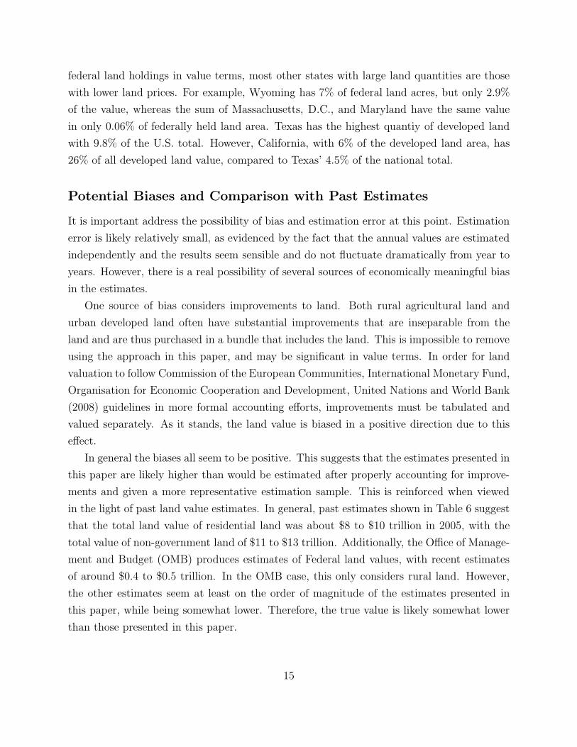
Table 1 shows the results of this model estimated for each year from 2000-2009. Parameter

estimates are fairly stable, suggesting a small degree of estimation error because these are

independent draws from the same sample of tracts. The one major exception is median value,

with estimated α1t rising from about 0.85 in the early years up to about 1.10 in the later

ones. Were this a structural model, this parameter non-constancy would be a major cause

for concern. However, because of the reduced-form, interpolatory nature of the exercise, the

signs and the R2 values are the most important. All signs are consistent with predictions

and each model explains over 2/3 of the variation in land prices, indicating a very high fit

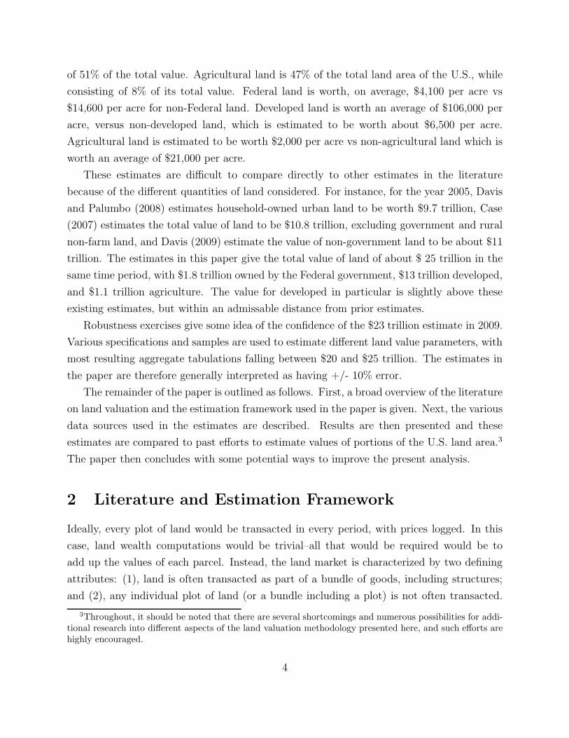
for a cross-sectional model. This is reflected in Figure 2, which shows the land price on the

6When the census tract is unpopulated, this interpolation of urban land is not used. Instead, land valuetabulations are based on agricultural land values.

7It would be desirable to include a construction cost index for PS , but due to the reliance on within-cityvariation for parameter estimation, and the fact that construction cost indices are usually at the city level(including R.S. Means), this variable is omitted.

8

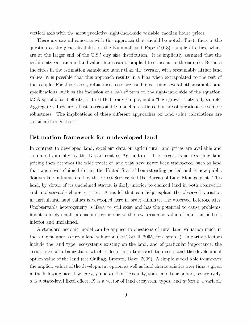
vertical axis with the most predictive right-hand-side variable, median house prices.

There are several concerns with this approach that should be noted. First, there is the

question of the generalizability of the Kuminoff and Pope (2013) sample of cities, which

are at the larger end of the U.S.’ city size distribution. It is implicitly assumed that the

within-city variation in land value shares can be applied to cities not in the sample. Because

the cities in the estimation sample are larger than the average, with presumably higher land

values, it is possible that this approach results in a bias when extrapolated to the rest of

the sample. For this reason, robustness tests are conducted using several other samples and

specifications, such as the inclusion of a value2 term on the right-hand side of the equation,

MSA-specific fixed effects, a “Rust Belt” only sample, and a “high growth” city only sample.

Aggregate values are robust to reasonable model alterations, but are of questionable sample

robustness. The implications of these different approaches on land value calculations are

considered in Section 4.

Estimation framework for undeveloped land

In contrast to developed land, excellent data on agricultural land prices are available and

computed annually by the Department of Agriculture. The largest issue regarding land

pricing then becomes the wide tracts of land that have never been transacted, such as land

that was never claimed during the United States’ homesteading period and is now public

domain land administered by the Forest Service and the Bureau of Land Management. This

land, by virtue of its unclaimed status, is likely inferior to claimed land in both observable

and unobservable characteristics. A model that can help explain the observed variation

in agricultural land values is developed here in order eliminate the observed heterogeneity.

Unobservable heterogeneity is likely to still exist and has the potential to cause problems,

but it is likely small in absolute terms due to the low presumed value of land that is both

inferior and unclaimed.

A standard hedonic model can be applied to questions of rural land valuation much in

the same manner as urban land valuation (see Torrell, 2005, for example). Important factors

include the land type, ecosystems existing on the land, and of particular importance, the

area’s level of urbanization, which reflects both transportation costs and the development

option value of the land (see Guiling, Brorsen, Doye, 2009). A simple model able to uncover

the implicit values of the development option as well as land characteristics over time is given

in the following model, where i, j, and t index the county, state, and time period, respectively,

α is a state-level fixed effect, X is a vector of land ecosystem types, and urban is a variable

9

measuring the “urbanness” of the county in terms of its population and proximity to other

population centers.

Vijt = αjt +X ′ijtβjt + γjturbanijt + εijt (5)

This model is estimated using observed agricultural land prices and characteristics. Land

prices for Federal land are then interpolated based on these estimated hedonic coefficients

and observed characteristics.

3 Data

The data used to apply the methods in the prior section of estimating both urban and rural

land prices are from a variety of public and private sources. These data include real estate

listings data, satellite imagery, Census Bureau and Department of Agriculture surveys and

tabulations, the General Service Administration’s Federal Real Property Profile database,

tax assessment data, and several GIS shapefiles.

National Land Cover Database

The National Land Cover Database (NLCD) consists of coded satellite imagery with a reso-

lution of 30m × 30m. This dataset is produced by the United States Geological Survey every

five years. The most recent release is 2006. For more information see Homer et al. (2004)

and Fry et al. (2011). The NLCD is a raster with 16 different land cover classifications,

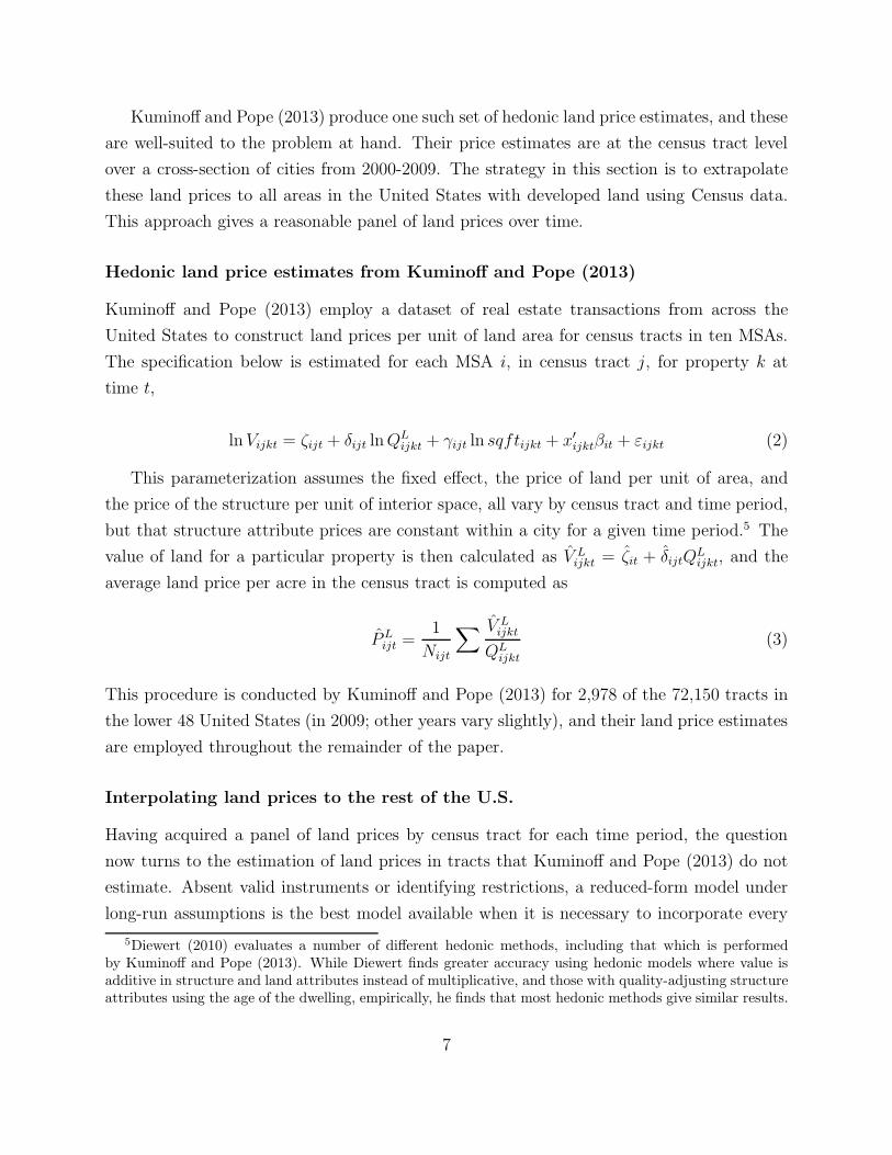
following the Anderson Land Cover Classification System (Anderson, 1976). For an example

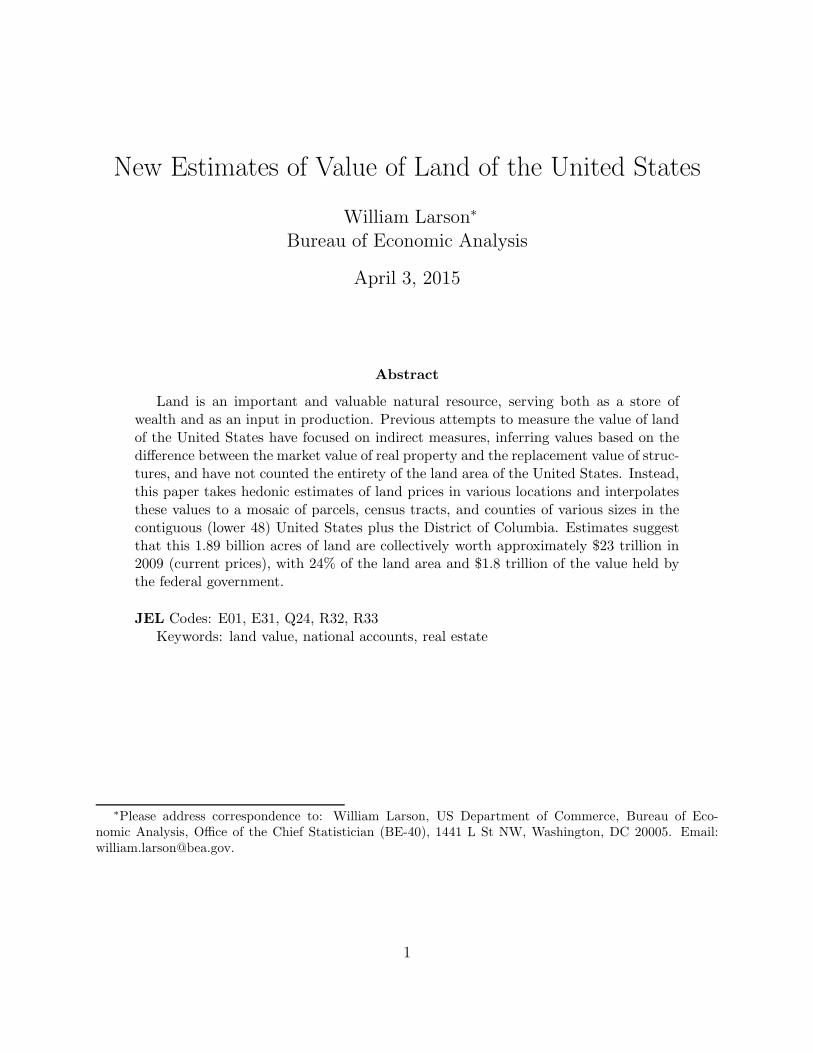
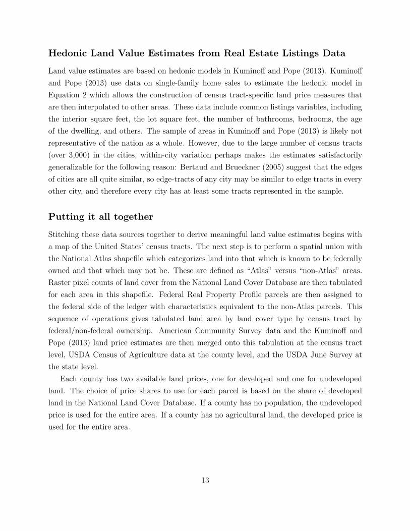
of the information in the NLCD, see Figure 1 for land classifications around the White Sands

Missile Range in New Mexico. This figure shows the center region which is barren due to

missile testing, along with areas of development (shades of red), grassland, and scrubland

(yellow-brown), and forest (green). The exceptional resolution of this database allows for

accurate tabulations of land types at small levels of geography.

National Atlas

The National Atlas is a division within the Department of the Interior. It produces GIS

shapefiles of different maps, including a map of all Federal and Indian lands with an area

greater than 640 acres (1 square mile). A spatial union of a U.S. county map with the map

of Federal and Indian lands produces a map with U.S. counties divided into non-Federal land

and Federal land by administering agency.

10

The National Atlas map on Federal lands is best used for large, rural land plots. While

items such as naval bases and national monuments appear reasonably defined in the data,

even for urban areas, the file misses smaller parcels. This necessitates the use of the Federal

Real Property Profile database of smaller parcels owned by the federal government.

Federal Real Property Profile

The Federal Real Property Profile (FRPP) is a database created by the General Services

Administration (GSA) in accordance with Executive Order 13327 of February, 2004. This

includes all land and buildings that are owned or leased by the Federal Government, with the

exception of public domain land and national parks and wildlife refuges. The FRPP includes

information on 34,126 parcels. Because the National Atlas includes all land areas greater than

1 square mile (640 acres), all properties with a land area of 600 acres or greater are omitted.

At this threshold, duplication between the data sources is minimal without erroneously

dropping unique parcels in the FRPP database. This filter leaves 32,447 parcels totaling

1,401,798 acres (2,190 sq. mi.). This database misses agencies not subject to appropriation

such as the Federal Reserve Board and the Securities and Exchange Commission, but is close

to the universe of all small federally held properties.

Tax assessor data

Washington, DC has a publicly available parcel database with separate tax assessments for

land and structures. Many parcel databases exist for other areas as well, but the time

cost of fully implementing a parcel-based approach is cost-prohibitive.8 Because of the

prevalence of federally owned parcels in the District, and the superiority of this source

compared to the Federal Real Property Profile, which misses certain parcels owned by the

U.S. government, the DC parcel database is the employed in this area. There are certainly

issues with appraisals, including documented biases in agricultural land appraisals according

to Ma and Swinton (2012). Additionally, appraisals may have other idiosyncrasies that cause

estimates to depart from true values, such timing lags between appraisals or the methods

of the land value appraisals themselves, which must be estimated. Urban land that is not

subject to taxation also may have biases because the tension in the desire for high versus

low appraisals from the assessor versus the property owner paying taxes does not exist.

8The cost and feasibility of a national parcel database has been investigated by Folger (2011) and U.S.Department of Housing and Urban Development, Office of Policy Development and Research (2013).

11

Ownership in the District is established by the owner name of the property. A sequence

of key words such as “United States of America,” “Forest Service,” “National Park Service”

and others are used as search phrases against the parcel database, with properties matching

the name attributed to the Federal government. In the District of Columbia parcel database,

2,727 of the 136,459 parcels are owned by the Federal government as of 2012, for a total of

7,279 acres, compared to 4,470 acres in the FRPP and National Atlas. Therefore, it is

crucial, at least in the District, to use a parcel database to calculate a reasonable value of

federal land.

USDA Census of Agriculture and June Survey

The Census of Agriculture is performed every five years by NASS, and measures farm prices

by farm land type by county. This data provides useful information on undeveloped land

prices over space. While the Census of Agriculture is every five years, there also exists an

annual survey at the state level, called the June Area Survey, also produced by NASS. This

survey contains land prices by crop land type. Using the Census county-level variation in

prices, along with the June Area Survey’s state-level land prices in each year, it is possible

to calculate land value by crop land type for each year in each county. The disaggregated

NASS agricultural land values are constructed net of large improvements such as structures,

but may include improvements such as fences, wells, grading, and biological capital such

as orchards or alfalfa root systems. These non-structure improvements confound the land

values, and further work should account for this fact.

American Community Survey

The American Community Survey is an annual survey of households performed by the Census

Bureau. This survey includes information on demographics, housing units, commuting, and

other socioeconomic indicators. Summary data are publicly available at the Census tract

level using a 5-year rolling sample. Census tracts are geographic areas that are meant to be

relatively stable over time, and consist of 1,000 to 8,000 people, with an ideal size of 4,000.

Because information exists on all census tracts, this is the ideal dataset for interpolation of

a representative sample of areas to the entirety of the United States.

12

Hedonic Land Value Estimates from Real Estate Listings Data

Land value estimates are based on hedonic models in Kuminoff and Pope (2013). Kuminoff

and Pope (2013) use data on single-family home sales to estimate the hedonic model in

Equation 2 which allows the construction of census tract-specific land price measures that

are then interpolated to other areas. These data include common listings variables, including

the interior square feet, the lot square feet, the number of bathrooms, bedrooms, the age

of the dwelling, and others. The sample of areas in Kuminoff and Pope (2013) is likely not

representative of the nation as a whole. However, due to the large number of census tracts

(over 3,000) in the cities, within-city variation perhaps makes the estimates satisfactorily

generalizable for the following reason: Bertaud and Brueckner (2005) suggest that the edges

of cities are all quite similar, so edge-tracts of any city may be similar to edge tracts in every

other city, and therefore every city has at least some tracts represented in the sample.

Putting it all together

Stitching these data sources together to derive meaningful land value estimates begins with

a map of the United States’ census tracts. The next step is to perform a spatial union with

the National Atlas shapefile which categorizes land into that which is known to be federally

owned and that which may not be. These are defined as “Atlas” versus “non-Atlas” areas.

Raster pixel counts of land cover from the National Land Cover Database are then tabulated

for each area in this shapefile. Federal Real Property Profile parcels are then assigned to

the federal side of the ledger with characteristics equivalent to the non-Atlas parcels. This

sequence of operations gives tabulated land area by land cover type by census tract by

federal/non-federal ownership. American Community Survey data and the Kuminoff and

Pope (2013) land price estimates are then merged onto this tabulation at the census tract

level, USDA Census of Agriculture data at the county level, and the USDA June Survey at

the state level.

Each county has two available land prices, one for developed and one for undeveloped

land. The choice of price shares to use for each parcel is based on the share of developed

land in the National Land Cover Database. If a county has no population, the undeveloped

price is used for the entire area. If a county has no agricultural land, the developed price is

used for the entire area.

13

4 Results

The methods in the prior section are applied from 2000-2009, which is the time over which

hedonic estimates exist in Kuminoff and Pope (2013). Overall results are encouraging, as

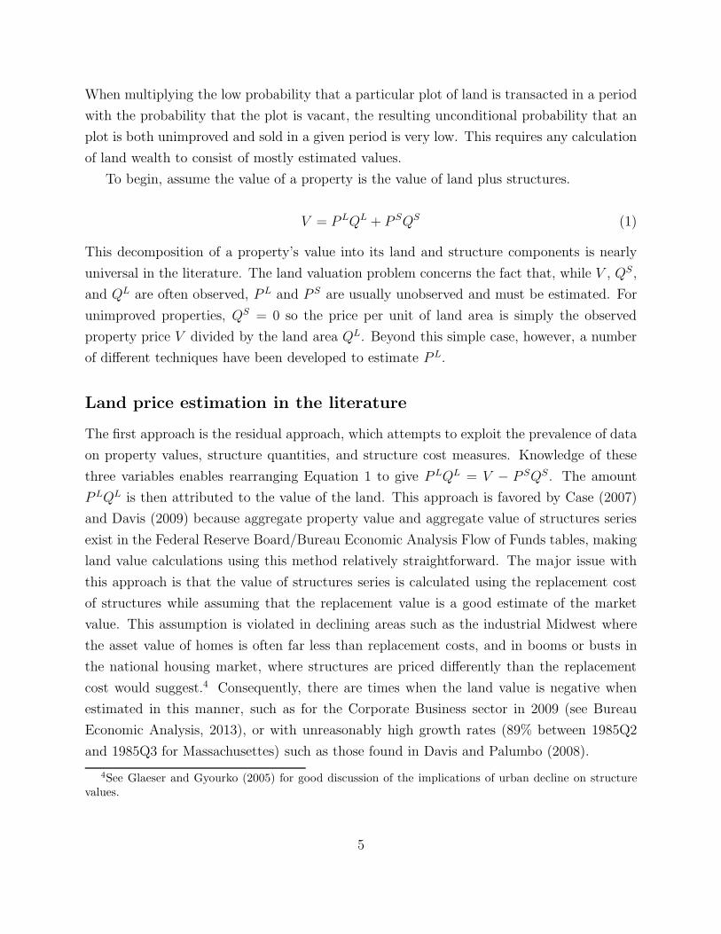
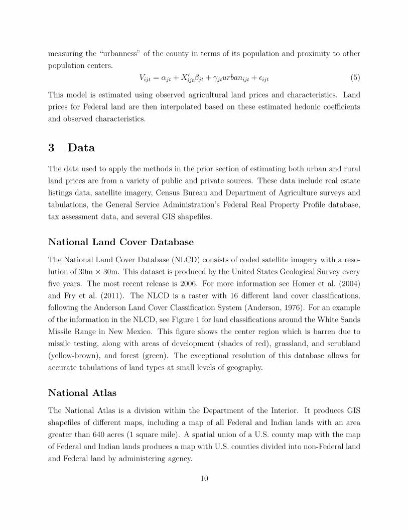
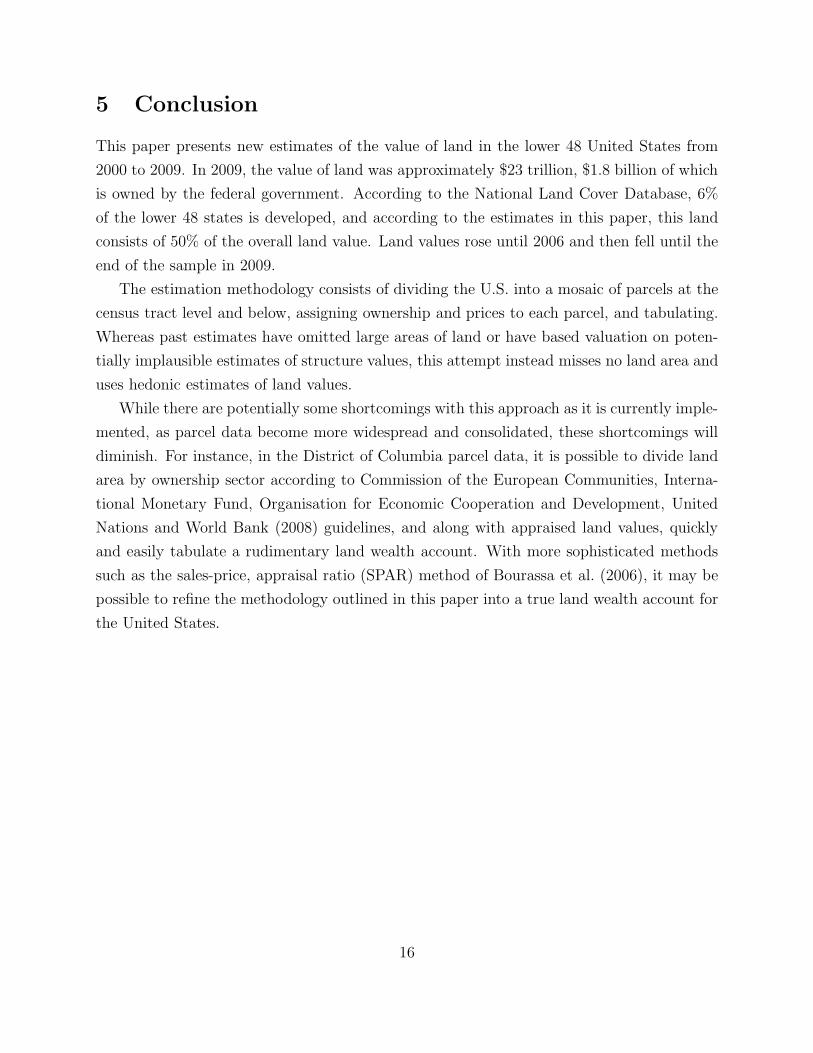
they follow the general trends in land prices expected over the decade. Figure 3 shows that

from 2000-2006, the value rose 26% from $20.1 trillion to $26.2 trillion, after which, from

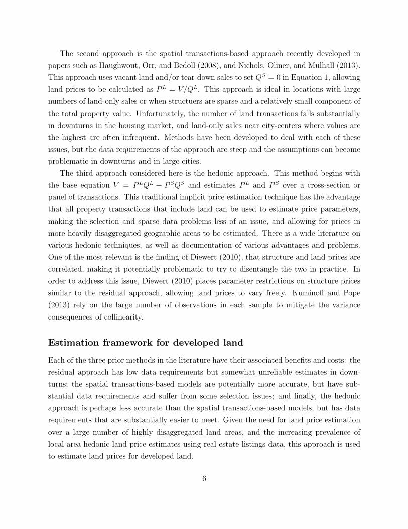
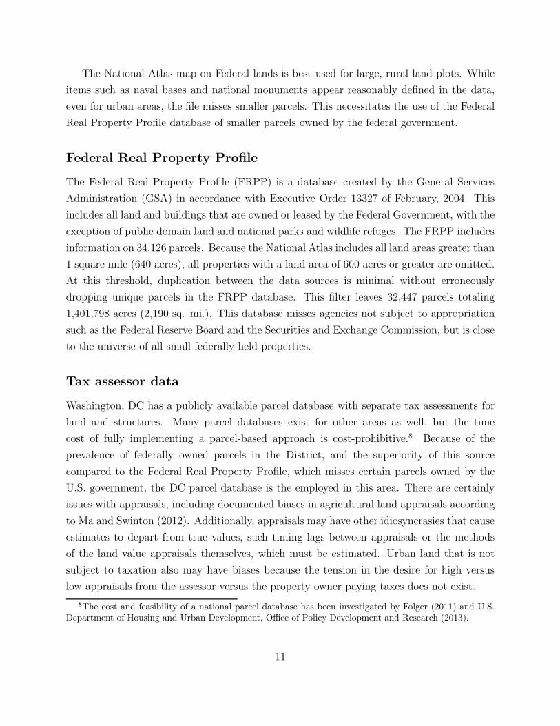
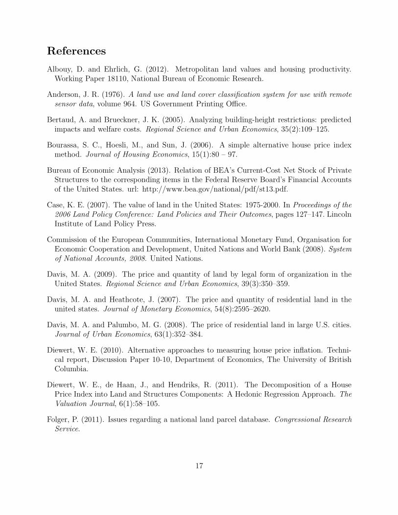
2006-2009, it fell 12% to $22.9 trillion. Figure 6 shows the spatial distribution of land value

per acre (land “prices”). This figure shows higher land prices in the east, west, and midwest

regions; population centers; and forested areas of the Rocky Mountains.

As Table 3 indicates, of the 1.89 billion acres in the lower 48 states, 24% of the land area

and 8% of the value is owned by the federal government, and 6% of the area and 51% of

the value is consists of developed land. Agricultural land is 47% of the total land area of

the U.S., while consisting of 8% of its total value. These shares do not sum to one because

they are not mutually exclusive. For instance the Federal government owns a large amount

of developed and agricultural land. Federal land is worth, on average, $4,100 per acre vs

$14,600 per acre for non-Federal land. Developed land is worth an average of $106,000 per

acre, versus non-developed land, which is estimated to be worth about $6,500 per acre.

Agricultural land is estimated to be worth $2,000 per acre vs non-agricultural land which is

worth an average of $21,000 per acre.

This table also shows that, within states, a great deal of variation is seen in land acres,

land value, and the quantity and value of both federal and developed land. California is the

most valuable state by a large margin, worth approximately $3.9 trillion in 2009. The lowest

average land value is Wyoming, with 62 million acres worth about $90 billion. 87% of the

land area of Nevada is owned by the federal government, but this land is only worth 45%

of the land value in the state due to the fact that much of the federal land is undeveloped

pasture. The most developed “state” is the District of Columbia, with 87% of its land

area covered by roads or buildings. Rhode Island and New Jersey are both 31% developed.

Several states have just 1% developed land, including Wyoming, New Mexico, Montana, and

Nevada. There are 6 states with over 80% agriculture land: Oklahoma, Iowa, Kansas, North

and South Dakota, and Nebraska. The states with under 10% of their land dedicated to

agriculture are the District of Columbia, Maine, Nevada, and New Hampshire.

Table 4 gives how much a particular state represents of the total area and value amounts.

60% of all federal land is concentrated in 7 states: Nevada (12%), California (10%), Arizona

(10%), Montana (7%), Idaho (7%), and Utah (7%), and New Mexico (7%). The value of

federal land is much more evenly distributed. While California makes up 18% of the nation’s

14

federal land holdings in value terms, most other states with large land quantities are those

with lower land prices. For example, Wyoming has 7% of federal land acres, but only 2.9%

of the value, whereas the sum of Massachusetts, D.C., and Maryland have the same value

in only 0.06% of federally held land area. Texas has the highest quantiy of developed land

with 9.8% of the U.S. total. However, California, with 6% of the developed land area, has

26% of all developed land value, compared to Texas’ 4.5% of the national total.

Potential Biases and Comparison with Past Estimates

It is important address the possibility of bias and estimation error at this point. Estimation

error is likely relatively small, as evidenced by the fact that the annual values are estimated

independently and the results seem sensible and do not fluctuate dramatically from year to

years. However, there is a real possibility of several sources of economically meaningful bias

in the estimates.

One source of bias considers improvements to land. Both rural agricultural land and

urban developed land often have substantial improvements that are inseparable from the

land and are thus purchased in a bundle that includes the land. This is impossible to remove

using the approach in this paper, and may be significant in value terms. In order for land

valuation to follow Commission of the European Communities, International Monetary Fund,

Organisation for Economic Cooperation and Development, United Nations and World Bank

(2008) guidelines in more formal accounting efforts, improvements must be tabulated and

valued separately. As it stands, the land value is biased in a positive direction due to this

effect.

In general the biases all seem to be positive. This suggests that the estimates presented in

this paper are likely higher than would be estimated after properly accounting for improve-

ments and given a more representative estimation sample. This is reinforced when viewed

in the light of past land value estimates. In general, past estimates shown in Table 6 suggest

that the total land value of residential land was about $8 to $10 trillion in 2005, with the

total value of non-government land of $11 to $13 trillion. Additionally, the Office of Manage-

ment and Budget (OMB) produces estimates of Federal land values, with recent estimates

of around $0.4 to $0.5 trillion. In the OMB case, this only considers rural land. However,

the other estimates seem at least on the order of magnitude of the estimates presented in

this paper, while being somewhat lower. Therefore, the true value is likely somewhat lower

than those presented in this paper.

15

5 Conclusion

This paper presents new estimates of the value of land in the lower 48 United States from

2000 to 2009. In 2009, the value of land was approximately $23 trillion, $1.8 billion of which

is owned by the federal government. According to the National Land Cover Database, 6%

of the lower 48 states is developed, and according to the estimates in this paper, this land

consists of 50% of the overall land value. Land values rose until 2006 and then fell until the

end of the sample in 2009.

The estimation methodology consists of dividing the U.S. into a mosaic of parcels at the

census tract level and below, assigning ownership and prices to each parcel, and tabulating.

Whereas past estimates have omitted large areas of land or have based valuation on poten-

tially implausible estimates of structure values, this attempt instead misses no land area and

uses hedonic estimates of land values.

While there are potentially some shortcomings with this approach as it is currently imple-

mented, as parcel data become more widespread and consolidated, these shortcomings will

diminish. For instance, in the District of Columbia parcel data, it is possible to divide land

area by ownership sector according to Commission of the European Communities, Interna-

tional Monetary Fund, Organisation for Economic Cooperation and Development, United

Nations and World Bank (2008) guidelines, and along with appraised land values, quickly

and easily tabulate a rudimentary land wealth account. With more sophisticated methods

such as the sales-price, appraisal ratio (SPAR) method of Bourassa et al. (2006), it may be

possible to refine the methodology outlined in this paper into a true land wealth account for

the United States.

16

References

Albouy, D. and Ehrlich, G. (2012). Metropolitan land values and housing productivity.Working Paper 18110, National Bureau of Economic Research.

Anderson, J. R. (1976). A land use and land cover classification system for use with remotesensor data, volume 964. US Government Printing Office.

Bertaud, A. and Brueckner, J. K. (2005). Analyzing building-height restrictions: predictedimpacts and welfare costs. Regional Science and Urban Economics, 35(2):109–125.

Bourassa, S. C., Hoesli, M., and Sun, J. (2006). A simple alternative house price indexmethod. Journal of Housing Economics, 15(1):80 – 97.

Bureau of Economic Analysis (2013). Relation of BEA’s Current-Cost Net Stock of PrivateStructures to the corresponding items in the Federal Reserve Board’s Financial Accountsof the United States. url: http://www.bea.gov/national/pdf/st13.pdf.

Case, K. E. (2007). The value of land in the United States: 1975-2000. In Proceedings of the2006 Land Policy Conference: Land Policies and Their Outcomes, pages 127–147. LincolnInstitute of Land Policy Press.

Commission of the European Communities, International Monetary Fund, Organisation forEconomic Cooperation and Development, United Nations and World Bank (2008). Systemof National Accounts, 2008. United Nations.

Davis, M. A. (2009). The price and quantity of land by legal form of organization in theUnited States. Regional Science and Urban Economics, 39(3):350–359.

Davis, M. A. and Heathcote, J. (2007). The price and quantity of residential land in theunited states. Journal of Monetary Economics, 54(8):2595–2620.

Davis, M. A. and Palumbo, M. G. (2008). The price of residential land in large U.S. cities.Journal of Urban Economics, 63(1):352–384.

Diewert, W. E. (2010). Alternative approaches to measuring house price inflation. Techni-cal report, Discussion Paper 10-10, Department of Economics, The University of BritishColumbia.

Diewert, W. E., de Haan, J., and Hendriks, R. (2011). The Decomposition of a HousePrice Index into Land and Structures Components: A Hedonic Regression Approach. TheValuation Journal, 6(1):58–105.

Folger, P. (2011). Issues regarding a national land parcel database. Congressional ResearchService.

17

Fry, J., Xian, G., Jin, S., Dewitz, J., Homer, C., Yang, L., Barnes, C., Herold, N., and Wick-ham, J. (2011). Completion of the 2006 national land cover database for the conterminousunited states. PERS, 77(9):858–864.

Glaeser, E. L. and Gyourko, J. (2005). Urban decline and durable housing. Journal ofPolitical Economy, 113(2):345–375.

Guiling, P., Brorsen, B. W., and Doye, D. (2009). Effect of urban proximity on agriculturalland values. Land Economics, 85(2):252–264.

Haughwout, A., Orr, J., and Bedoll, D. (2008). The price of land in the New York metropoli-tan area. Federal Reserve Bank of New York: Current Issues in Economics and Finance,14(3).

Homer, C., Huang, C., Yang, L., Wylie, B., and Coan, M. (2004). Development of a 2001national land-cover database for the United States. Photogrammetric Engineering andRemote Sensing, 70(7):829–840.

Jorgenson, D. W., Landefeld, J. S., and Nordhaus, W. D. (2006). A new architecture for theUS national accounts, volume 66. University of Chicago Press.

Kuminoff, N. V. and Pope, J. C. (2013). The value of residential land and structures duringthe great housing boom and bust. Land Economics, 89(1):1–29.

Ma, S. and Swinton, S. M. (2012). Hedonic valuation of farmland using sale prices versusappraised values. Land Economics, 88(1):1–15.

Nichols, J. B., Oliner, S. D., and Mulhall, M. R. (2013). Swings in commercial and residentialland prices in the United States. Journal of Urban Economics, 73(1):57 – 76.

Office of Management and Budget (2012). Fiscal Year 2013: Analytical Perspectives. U.S.Government Printing Office.

Torell, L. A., Rimbey, N. R., Ramirez, O. A., and McCollum, D. W. (2005). Income earn-ing potential versus consumptive amenities in determining ranchland values. Journal ofAgricultural and Resource Economics, pages 537–560.

U.S. Department of Housing and Urban Development, Office of Policy Development andResearch (2013). The feasibility of developing a national parcel database: County datarecords project final report. Technical report.

18

Figure 1: White Sands Missile Range, NM, Land Cover, 2006

White Sands Missi le Range

Lincoln National Forest

Fort Bl iss McGregor Range

Mescalero Apache Indian Reservation

White Sands National Mounument

Hol loman Air Force Base

19

Figure 2: Results of Land Value Interpolation from Kuminoff and Pope (2013) using Census(ACS) data, 2009

810

1214

1618

Est

imat

ed L

and

Pric

e pe

r ac

re (

log)

9 10 11 12 13 14Median Home Value (ACS, log)

ACS Interpolation Kuminoff and Pope (2013) Estimate

20

Figure 3: Land Value of the Lower 48 States, 2000-2009

2022

2426

2830

$ tr

illio

n (c

urre

nt)

2000 2001 2002 2003 2004 2005 2006 2007 2008 2009

21

Figure 4: Land Value of the Lower 48 States, 2000-2009, Model Robustness

2025

3035

2000 2002 2004 2006 2008 2010year

Baseline Med. Value Only Age QuadraticValue Quadratic No Density No Dwelling AgeNo Rooms

22

Figure 5: Land Value of the Lower 48 States, 2000-2009, Sample Robustness

2022

2426

2830

2000 2002 2004 2006 2008 2010year

Baseline Rust Belt Non−Rust Belt

23

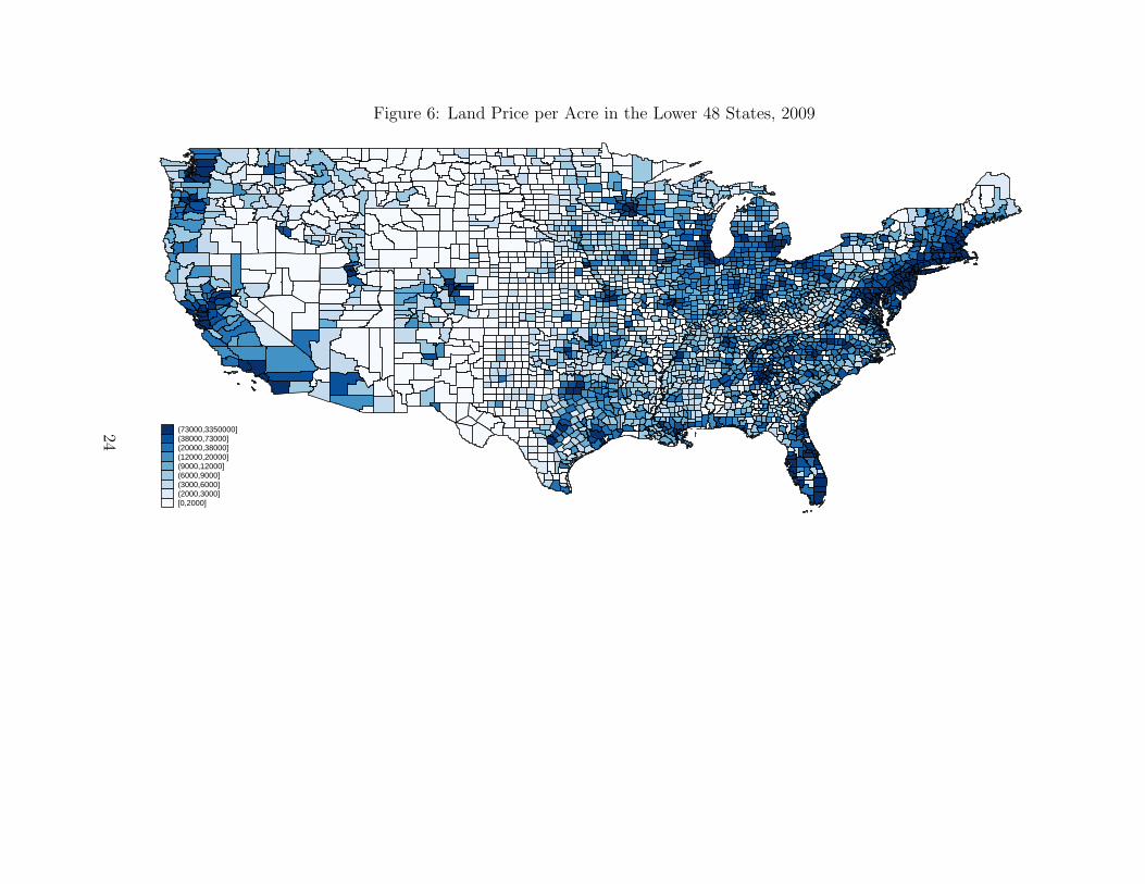
Figure 6: Land Price per Acre in the Lower 48 States, 2009

(73000,3350000](38000,73000](20000,38000](12000,20000](9000,12000](6000,9000](3000,6000](2000,3000][0,2000]

24

Table 1: Land price interpolation estimates

Dependent variable: Land Price per Acre (log)

Year 2000 2001 2002 2003 2004 2005 2006 2007 2008 2009

Property Value 0.908*** 0.905*** 0.942*** 0.930*** 1.048*** 1.099*** 1.121*** 1.095*** 1.125*** 1.164***(0.0210) (0.0206) (0.0201) (0.0193) (0.0192) (0.0193) (0.0199) (0.0202) (0.0211) (0.0226)

Rooms -0.148*** -0.162*** -0.171*** -0.175*** -0.202*** -0.220*** -0.244*** -0.219*** -0.183*** -0.177***(0.0150) (0.0147) (0.0143) (0.0137) (0.0137) (0.0138) (0.0142) (0.0144) (0.0150) (0.0161)

Tract Density 0.303*** 0.283*** 0.293*** 0.294*** 0.310*** 0.323*** 0.344*** 0.333*** 0.289*** 0.284***(0.0158) (0.0155) (0.0151) (0.0145) (0.0145) (0.0145) (0.0150) (0.0152) (0.0159) (0.0170)

Age of Housing Unit 0.375*** 0.357*** 0.336*** 0.348*** 0.297*** 0.272*** 0.183*** 0.261*** 0.346*** 0.435***(0.0373) (0.0367) (0.0356) (0.0342) (0.0341) (0.0343) (0.0354) (0.0359) (0.0374) (0.0401)

Constant 0.692** 1.033*** 0.755** 1.004*** -0.0511 -0.406 -0.210 -0.326 -1.366*** -2.301***(0.311) (0.306) (0.297) (0.286) (0.285) (0.286) (0.295) (0.300) (0.312) (0.335)

Observations 1,917 1,917 1,918 1,919 1,919 1,917 1,917 1,919 1,917 1,916R-squared 0.659 0.660 0.686 0.703 0.739 0.755 0.752 0.738 0.715 0.699

Notes: Standard errors in parentheses. *** p < 0.01, ** p < 0.05, * p < 0.1. Property Value, Rooms, and Age of Housing Unit are medians;Property Value, Tract Density, and Age of Housing Unit are in logs. The table presents reduced-form models of land prices. Models are estimatedseparately for each year.

25

Table 2: Land Quantities and Values by Sector: Washington, DC, 2013

Acres Value P/Acre

Households and NPISH 14,431 $ 26,691,233,792 $ 1,849,604Non-Financial, Non-Corporate Business 5,019 $ 33,426,939,179 $ 6,660,575Non-Financial, Corporate Business 2,985 $ 9,667,046,481 $ 3,238,784Financial Business 249 $ 1,823,793,668 $ 7,315,267State and Local Government 2,578 $ 8,029,715,968 $ 3,114,669Federal Government 7,279 $ 29,549,412,352 $ 4,059,712

Total 32,540 $ 109,188,141,440 $ 3,355,482

26

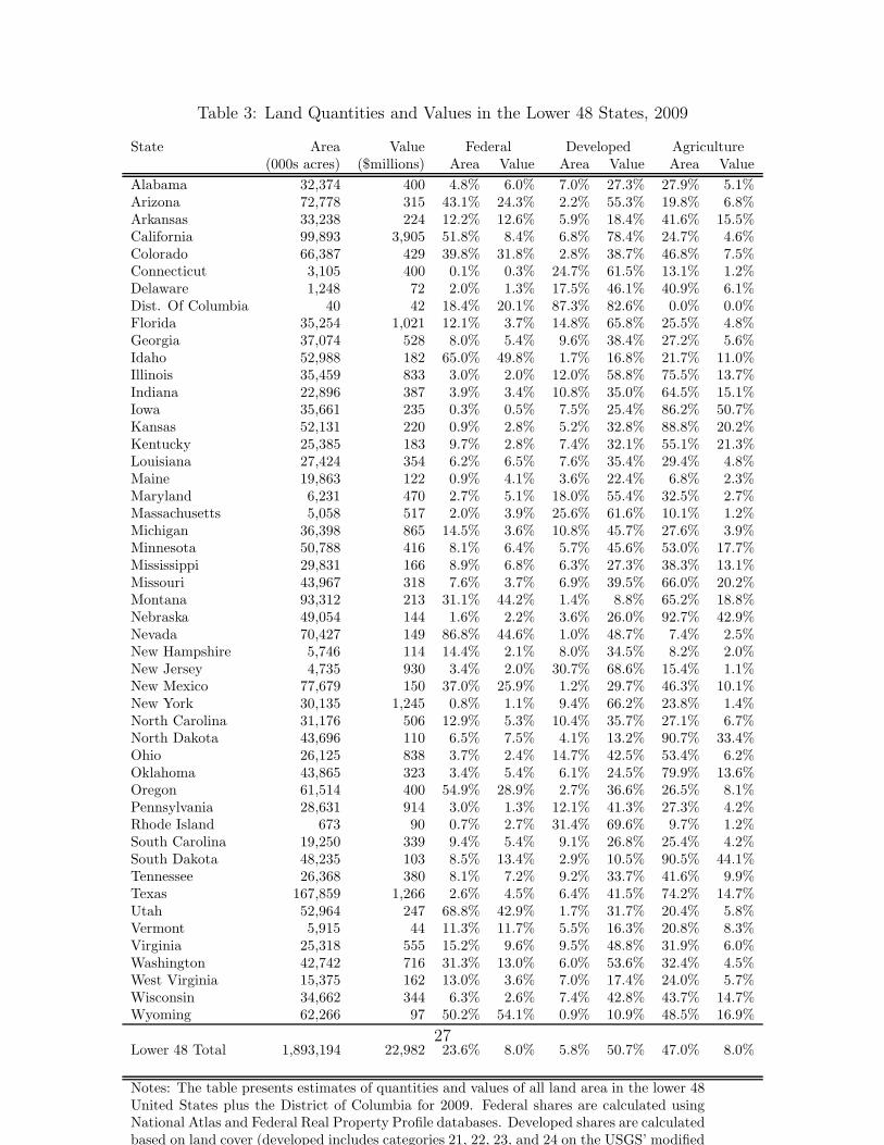
Table 3: Land Quantities and Values in the Lower 48 States, 2009

State Area Value Federal Developed Agriculture(000s acres) ($millions) Area Value Area Value Area Value

Alabama 32,374 400 4.8% 6.0% 7.0% 27.3% 27.9% 5.1%Arizona 72,778 315 43.1% 24.3% 2.2% 55.3% 19.8% 6.8%Arkansas 33,238 224 12.2% 12.6% 5.9% 18.4% 41.6% 15.5%California 99,893 3,905 51.8% 8.4% 6.8% 78.4% 24.7% 4.6%Colorado 66,387 429 39.8% 31.8% 2.8% 38.7% 46.8% 7.5%Connecticut 3,105 400 0.1% 0.3% 24.7% 61.5% 13.1% 1.2%Delaware 1,248 72 2.0% 1.3% 17.5% 46.1% 40.9% 6.1%Dist. Of Columbia 40 42 18.4% 20.1% 87.3% 82.6% 0.0% 0.0%Florida 35,254 1,021 12.1% 3.7% 14.8% 65.8% 25.5% 4.8%Georgia 37,074 528 8.0% 5.4% 9.6% 38.4% 27.2% 5.6%Idaho 52,988 182 65.0% 49.8% 1.7% 16.8% 21.7% 11.0%Illinois 35,459 833 3.0% 2.0% 12.0% 58.8% 75.5% 13.7%Indiana 22,896 387 3.9% 3.4% 10.8% 35.0% 64.5% 15.1%Iowa 35,661 235 0.3% 0.5% 7.5% 25.4% 86.2% 50.7%Kansas 52,131 220 0.9% 2.8% 5.2% 32.8% 88.8% 20.2%Kentucky 25,385 183 9.7% 2.8% 7.4% 32.1% 55.1% 21.3%Louisiana 27,424 354 6.2% 6.5% 7.6% 35.4% 29.4% 4.8%Maine 19,863 122 0.9% 4.1% 3.6% 22.4% 6.8% 2.3%Maryland 6,231 470 2.7% 5.1% 18.0% 55.4% 32.5% 2.7%Massachusetts 5,058 517 2.0% 3.9% 25.6% 61.6% 10.1% 1.2%Michigan 36,398 865 14.5% 3.6% 10.8% 45.7% 27.6% 3.9%Minnesota 50,788 416 8.1% 6.4% 5.7% 45.6% 53.0% 17.7%Mississippi 29,831 166 8.9% 6.8% 6.3% 27.3% 38.3% 13.1%Missouri 43,967 318 7.6% 3.7% 6.9% 39.5% 66.0% 20.2%Montana 93,312 213 31.1% 44.2% 1.4% 8.8% 65.2% 18.8%Nebraska 49,054 144 1.6% 2.2% 3.6% 26.0% 92.7% 42.9%Nevada 70,427 149 86.8% 44.6% 1.0% 48.7% 7.4% 2.5%New Hampshire 5,746 114 14.4% 2.1% 8.0% 34.5% 8.2% 2.0%New Jersey 4,735 930 3.4% 2.0% 30.7% 68.6% 15.4% 1.1%New Mexico 77,679 150 37.0% 25.9% 1.2% 29.7% 46.3% 10.1%New York 30,135 1,245 0.8% 1.1% 9.4% 66.2% 23.8% 1.4%North Carolina 31,176 506 12.9% 5.3% 10.4% 35.7% 27.1% 6.7%North Dakota 43,696 110 6.5% 7.5% 4.1% 13.2% 90.7% 33.4%Ohio 26,125 838 3.7% 2.4% 14.7% 42.5% 53.4% 6.2%Oklahoma 43,865 323 3.4% 5.4% 6.1% 24.5% 79.9% 13.6%Oregon 61,514 400 54.9% 28.9% 2.7% 36.6% 26.5% 8.1%Pennsylvania 28,631 914 3.0% 1.3% 12.1% 41.3% 27.3% 4.2%Rhode Island 673 90 0.7% 2.7% 31.4% 69.6% 9.7% 1.2%South Carolina 19,250 339 9.4% 5.4% 9.1% 26.8% 25.4% 4.2%South Dakota 48,235 103 8.5% 13.4% 2.9% 10.5% 90.5% 44.1%Tennessee 26,368 380 8.1% 7.2% 9.2% 33.7% 41.6% 9.9%Texas 167,859 1,266 2.6% 4.5% 6.4% 41.5% 74.2% 14.7%Utah 52,964 247 68.8% 42.9% 1.7% 31.7% 20.4% 5.8%Vermont 5,915 44 11.3% 11.7% 5.5% 16.3% 20.8% 8.3%Virginia 25,318 555 15.2% 9.6% 9.5% 48.8% 31.9% 6.0%Washington 42,742 716 31.3% 13.0% 6.0% 53.6% 32.4% 4.5%West Virginia 15,375 162 13.0% 3.6% 7.0% 17.4% 24.0% 5.7%Wisconsin 34,662 344 6.3% 2.6% 7.4% 42.8% 43.7% 14.7%Wyoming 62,266 97 50.2% 54.1% 0.9% 10.9% 48.5% 16.9%

Lower 48 Total 1,893,194 22,982 23.6% 8.0% 5.8% 50.7% 47.0% 8.0%

Notes: The table presents estimates of quantities and values of all land area in the lower 48United States plus the District of Columbia for 2009. Federal shares are calculated usingNational Atlas and Federal Real Property Profile databases. Developed shares are calculatedbased on land cover (developed includes categories 21, 22, 23, and 24 on the USGS’ modified

27

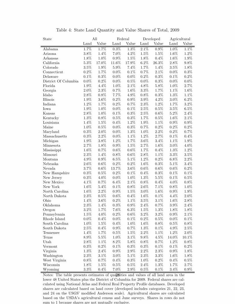
Table 4: State Land Quantity and Value Shares of Total, 2009

State All Federal Developed AgriculturalLand Value Land Value Land Value Land Value

Alabama 1.7% 1.7% 0.3% 1.3% 2.1% 0.9% 1.0% 1.1%Arizona 3.8% 1.4% 7.0% 4.2% 1.5% 1.5% 1.6% 1.2%Arkansas 1.8% 1.0% 0.9% 1.5% 1.8% 0.4% 1.6% 1.9%California 5.3% 17.0% 11.6% 17.9% 6.2% 26.3% 2.8% 9.8%Colorado 3.5% 1.9% 5.9% 7.4% 1.7% 1.4% 3.5% 1.8%Connecticut 0.2% 1.7% 0.0% 0.1% 0.7% 2.1% 0.0% 0.3%Delaware 0.1% 0.3% 0.0% 0.0% 0.2% 0.3% 0.1% 0.2%District Of Columbia 0.0% 0.2% 0.0% 0.5% 0.0% 0.3% 0.0% 0.0%Florida 1.9% 4.4% 1.0% 2.1% 4.8% 5.8% 1.0% 2.7%Georgia 2.0% 2.3% 0.7% 1.6% 3.3% 1.7% 1.1% 1.6%Idaho 2.8% 0.8% 7.7% 4.9% 0.8% 0.3% 1.3% 1.1%Illinois 1.9% 3.6% 0.2% 0.9% 3.9% 4.2% 3.0% 6.2%Indiana 1.2% 1.7% 0.2% 0.7% 2.3% 1.2% 1.7% 3.2%Iowa 1.9% 1.0% 0.0% 0.1% 2.5% 0.5% 3.5% 6.5%Kansas 2.8% 1.0% 0.1% 0.3% 2.5% 0.6% 5.2% 2.4%Kentucky 1.3% 0.8% 0.5% 0.3% 1.7% 0.5% 1.6% 2.1%Louisiana 1.4% 1.5% 0.4% 1.2% 1.9% 1.1% 0.9% 0.9%Maine 1.0% 0.5% 0.0% 0.3% 0.7% 0.2% 0.2% 0.2%Maryland 0.3% 2.0% 0.0% 1.3% 1.0% 2.2% 0.2% 0.7%Massachusetts 0.3% 2.2% 0.0% 1.1% 1.2% 2.7% 0.1% 0.4%Michigan 1.9% 3.8% 1.2% 1.7% 3.6% 3.4% 1.1% 1.9%Minnesota 2.7% 1.8% 0.9% 1.5% 2.7% 1.6% 3.0% 4.0%Mississippi 1.6% 0.7% 0.6% 0.6% 1.7% 0.4% 1.3% 1.2%Missouri 2.3% 1.4% 0.8% 0.6% 2.8% 1.1% 3.3% 3.5%Montana 4.9% 0.9% 6.5% 5.1% 1.2% 0.2% 6.8% 2.2%Nebraska 2.6% 0.6% 0.2% 0.2% 1.6% 0.3% 5.1% 3.4%Nevada 3.7% 0.6% 13.7% 3.6% 0.6% 0.6% 0.6% 0.2%New Hampshire 0.3% 0.5% 0.2% 0.1% 0.4% 0.3% 0.1% 0.1%New Jersey 0.3% 4.0% 0.0% 1.0% 1.3% 5.5% 0.1% 0.5%New Mexico 4.1% 0.7% 6.4% 2.1% 0.8% 0.4% 4.0% 0.8%New York 1.6% 5.4% 0.1% 0.8% 2.6% 7.1% 0.8% 1.0%North Carolina 1.6% 2.2% 0.9% 1.5% 3.0% 1.6% 0.9% 1.9%North Dakota 2.3% 0.5% 0.6% 0.4% 1.6% 0.1% 4.4% 2.0%Ohio 1.4% 3.6% 0.2% 1.1% 3.5% 3.1% 1.6% 2.8%Oklahoma 2.3% 1.4% 0.3% 0.9% 2.4% 0.7% 3.9% 2.4%Oregon 3.2% 1.7% 7.6% 6.3% 1.5% 1.3% 1.8% 1.8%Pennsylvania 1.5% 4.0% 0.2% 0.6% 3.2% 3.2% 0.9% 2.1%Rhode Island 0.0% 0.4% 0.0% 0.1% 0.2% 0.5% 0.0% 0.1%South Carolina 1.0% 1.5% 0.4% 1.0% 1.6% 0.8% 0.5% 0.8%South Dakota 2.5% 0.4% 0.9% 0.7% 1.3% 0.1% 4.9% 2.5%Tennessee 1.4% 1.7% 0.5% 1.5% 2.2% 1.1% 1.2% 2.0%Texas 8.9% 5.5% 1.0% 3.1% 9.8% 4.5% 14.0% 10.1%Utah 2.8% 1.1% 8.2% 5.8% 0.8% 0.7% 1.2% 0.8%Vermont 0.3% 0.2% 0.1% 0.3% 0.3% 0.1% 0.1% 0.2%Virginia 1.3% 2.4% 0.9% 2.9% 2.2% 2.3% 0.9% 1.8%Washington 2.3% 3.1% 3.0% 5.1% 2.3% 3.3% 1.6% 1.8%West Virginia 0.8% 0.7% 0.4% 0.3% 1.0% 0.2% 0.4% 0.5%Wisconsin 1.8% 1.5% 0.5% 0.5% 2.4% 1.3% 1.7% 2.7%Wyoming 3.3% 0.4% 7.0% 2.9% 0.5% 0.1% 3.4% 0.9%

Notes: The table presents estimates of quantities and values of all land area in thelower 48 United States plus the District of Columbia for 2009. Federal shares are cal-culated using National Atlas and Federal Real Property Profile databases. Developedshares are calculated based on land cover (developed includes categories 21, 22, 23,and 24 on the USGS’ modified Anderson scale). Agricultural shares are calculatedbased on the USDA’s agricultural census and June surveys. Shares in rows do notsum to 1 because shares are not mutually exclusive.

28

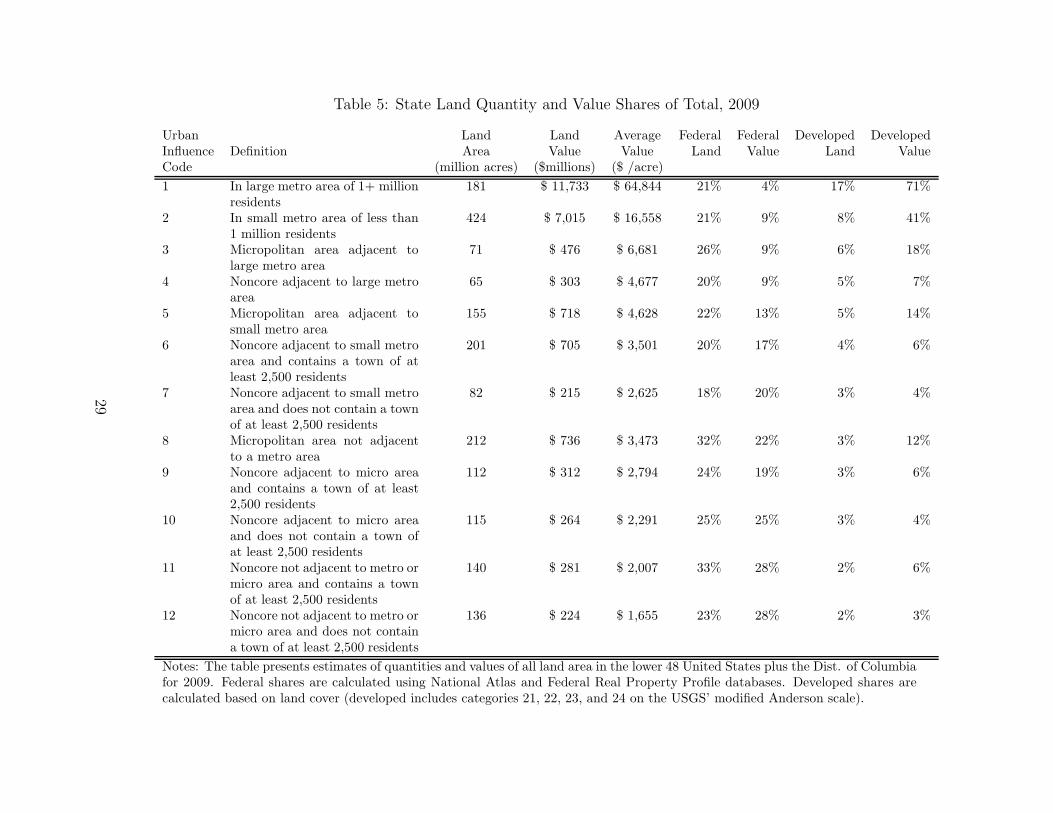
Table 5: State Land Quantity and Value Shares of Total, 2009

Urban Land Land Average Federal Federal Developed DevelopedInfluence Definition Area Value Value Land Value Land ValueCode (million acres) ($millions) ($ /acre)

1 In large metro area of 1+ millionresidents

181 $ 11,733 $ 64,844 21% 4% 17% 71%

2 In small metro area of less than1 million residents

424 $ 7,015 $ 16,558 21% 9% 8% 41%

3 Micropolitan area adjacent tolarge metro area

71 $ 476 $ 6,681 26% 9% 6% 18%

4 Noncore adjacent to large metroarea

65 $ 303 $ 4,677 20% 9% 5% 7%

5 Micropolitan area adjacent tosmall metro area

155 $ 718 $ 4,628 22% 13% 5% 14%

6 Noncore adjacent to small metroarea and contains a town of atleast 2,500 residents

201 $ 705 $ 3,501 20% 17% 4% 6%

7 Noncore adjacent to small metroarea and does not contain a townof at least 2,500 residents

82 $ 215 $ 2,625 18% 20% 3% 4%

8 Micropolitan area not adjacentto a metro area

212 $ 736 $ 3,473 32% 22% 3% 12%

9 Noncore adjacent to micro areaand contains a town of at least2,500 residents

112 $ 312 $ 2,794 24% 19% 3% 6%

10 Noncore adjacent to micro areaand does not contain a town ofat least 2,500 residents

115 $ 264 $ 2,291 25% 25% 3% 4%

11 Noncore not adjacent to metro ormicro area and contains a townof at least 2,500 residents

140 $ 281 $ 2,007 33% 28% 2% 6%

12 Noncore not adjacent to metro ormicro area and does not containa town of at least 2,500 residents

136 $ 224 $ 1,655 23% 28% 2% 3%

Notes: The table presents estimates of quantities and values of all land area in the lower 48 United States plus the Dist. of Columbiafor 2009. Federal shares are calculated using National Atlas and Federal Real Property Profile databases. Developed shares arecalculated based on land cover (developed includes categories 21, 22, 23, and 24 on the USGS’ modified Anderson scale).

29

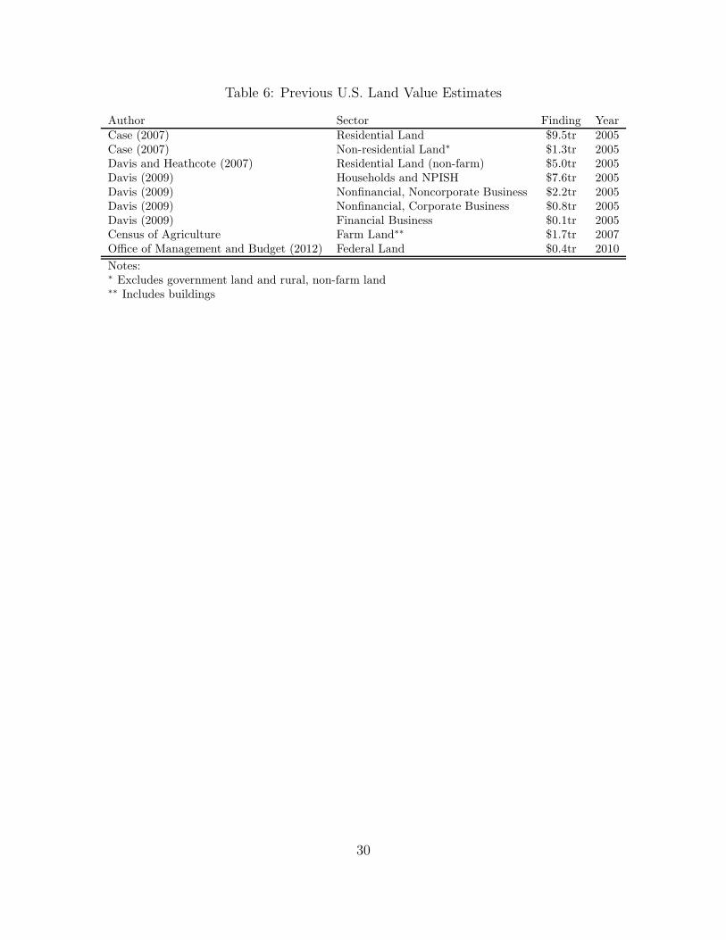
Table 6: Previous U.S. Land Value Estimates

Author Sector Finding YearCase (2007) Residential Land $9.5tr 2005Case (2007) Non-residential Land∗ $1.3tr 2005Davis and Heathcote (2007) Residential Land (non-farm) $5.0tr 2005Davis (2009) Households and NPISH $7.6tr 2005Davis (2009) Nonfinancial, Noncorporate Business $2.2tr 2005Davis (2009) Nonfinancial, Corporate Business $0.8tr 2005Davis (2009) Financial Business $0.1tr 2005Census of Agriculture Farm Land∗∗ $1.7tr 2007Office of Management and Budget (2012) Federal Land $0.4tr 2010

Notes:∗ Excludes government land and rural, non-farm land∗∗ Includes buildings

30