new fast integrated mobility spectrometer for real-time measurement of aerosol size...

Aerosol Science 37 (2006) 1303–1325www.elsevier.com/locate/jaerosci

New fast integrated mobility spectrometer for real-timemeasurement of aerosol size distribution—I: Concept and theory

Pramod Kulkarni, Jian Wang∗

Brookhaven National Laboratory, Building 815E, Upton, NY 11973-5000, USA

Received 15 November 2005; received in revised form 6 January 2006; accepted 17 January 2006

Abstract

A new instrument capable of measuring aerosol size distribution with high time and size resolution, and high signal-to-noise ratiois described. The instrument, referred to as Fast Integrated Mobility Spectrometer (FIMS), separates charged particles based on theirelectrical mobility into different trajectories in a uniform electric field. The particles are then grown into super-micrometer droplets,and their locations on the trajectories are recorded by a fast charge-coupled device (CCD) imaging system. Images captured bythe CCD reveal mobility-dependent particle positions and their numbers, which are then used to derive a particle size distributionspectrum. By eliminating the need to scan over a range of voltages, FIMS significantly improves the measurement speed and countingstatistics. A theoretical framework has been developed to quantify the measurement range, mobility resolution, and transfer functionof FIMS. It is shown that FIMS is capable of measuring aerosol size distributions with high-time and size resolution. 2006 Elsevier Ltd. All rights reserved.

Keywords: Aerosol size distribution measurements; High-time resolution; Electric mobility; Transfer function; Particle diffusion; Mobilityresolution

1. Introduction

Real-time measurement of particle size distributions, especially in the nanometer size range, is important in manyapplications such as measurement of atmospheric aerosols and characterization of particles in combustion systems.To capture transient aerosol dynamics occurring on very small time scales, such as in high-temperature environmentsor other nucleation-dominated systems, fast measurements are often necessary. In other types of measurements, suchas aircraft-based studies aimed at characterizing spatial and temporal distributions of atmospheric aerosols, high-timeresolution is required to capture variations of aerosol properties over a small spatial domain.

Sub-micrometer aerosol size distributions are mostly measured using electrical mobility techniques, especiallyfor particles with diameter less than 100 nm. There have been considerable advances in electrical mobility-based

This manuscript has been authored by Brookhaven Science Associates, LLC under Contract No. DE-AC02-98CH1-886 with the US Departmentof Energy. The United States Government retains, and the publisher, by accepting the article for publication, acknowledges, a world-wide license topublish or reproduce the published form of this manuscript, or allow others to do so, for the United States Government purposes.

∗ Corresponding author. Tel.: +1 631 344 7920; fax: +1 631 344 2887.E-mail address: [email protected] (J. Wang).

0021-8502/$ - see front matter 2006 Elsevier Ltd. All rights reserved.doi:10.1016/j.jaerosci.2006.01.005

http://www.elsevier.com/locate/jaerosci

mailto:[email protected]

1304 P. Kulkarni, J. Wang / Aerosol Science 37 (2006) 1303 –1325

measurements, from its early time-intensive days to the current state-of-the-art scanning mobility techniques thattake only a few minutes to characterize an entire size distribution spectrum (Flagan, 1998). Electrical mobility-basedmeasurement system often consists of two components: a Differential Mobility Analyzer (DMA) that selects particleswithin a narrow mobility window (Knutson & Whitby, 1975), and a detector that counts the number of particles withinthe classified window of mobility. In its early days, mobility-based measurements were made by stepping the classifyingvoltage of the DMA through a sequence of values to reproduce an entire size distribution, and the measurement timewas on the order of 10 min or more. Wang and Flagan (1989) introduced the scanning mobility technique in which theclassifying voltage of DMA is continuously scanned. As a result, the time required to measure aerosol size distributioncould be substantially reduced to about 1 min. Systems using the scanning mobility technique are often referred to asScanning Mobility Particle Sizers (SMPS).

There are two obstacles for further accelerating the SMPS measurements. First, faster measurements often resultin severely distorted size distributions, which are attributed to the large smearing effect of traditional condensationparticle counters (CPCs) used as detectors (Russell, Flagan, & Seinfeld, 1995). To reduce the smearing effect, thescanning mobility techniques have been augmented with time-sensitive detectors. Wang, McNeill, Collins, and Flagan(2002) developed a fast-response mixing condensation nucleus counter (MCNC). They reduced the measurementtime to about 3 s by using the MCNC as a detector in SMPS (Wang et al., 2002). The second obstacle to fasterSMPS measurements is the low sampling rate and the associated low counting statistics. SMPS systems are based on asequential measurement technique. Only particles within a narrow range of mobility, which comprise a small fraction ofthe total aerosol particles introduced into the instrument, are measured at a given time. Whereas, time-sensitive detectorsmay allow faster measurements, the low counting statistics often require averaging fast measurements over a longerperiod of time to obtain statistically significant results. This further effectively offsets the reduction in measurementtime gained by using the time-sensitive detectors. Other electrical mobility-based instruments include the ElectricalAerosol Spectrometer (EAS) developed by Mirme et al. (1984), (Mirme, 1994; Tammet, Mirme, & Tamm, 1998,2002). The EAS uses an array of integrated electrometers that operate in parallel in a DMA-like geometry. Sinceparticles of different mobilities are detected simultaneously, EAS is capable of sub-second measurements of aerosolsize distributions. Due to the relatively low sensitivity of the electrometers, application of EAS is limited to aerosols withhigh number concentrations. This instrument has been commercialized by TSI Inc. as Engine Exhaust Particle Sizer(EEPS), and is primarily used for characterizing high concentration engine exhausts (Johnson, Caldow, Pocher, Mirme,& Kittelson, 2004). Besides low sensitivity, EAS and EEPS also have considerably lower size resolution comparedto SMPS.

The other type of instruments that are frequently used to measure sub-micrometer aerosol size distributions are Opti-cal Particle Counters (OPCs). For OPC measurements, particle sizes are derived from the intensity of light scattered byparticles. OPC offer fast measurement speed and better counting statistics compared to SMPS. However, the measure-ment range of OPCs is limited to particles with diameters greater than 100 nm. Also, particle physical properties suchas shape, refractive index, and morphology have strong influences on derived particle sizes, and are often unavailable.Even for the ideal case of homogeneous spherical aerosol particles, the uncertainty in refractive index often leads tosignificant uncertainties in derived size distributions (Hering & McMurry, 1991). Furthermore, the interpretation ofOPC data is often complicated by Mie resonances in the intensity of light scattered by spherical particles.

Besides SMPS and OPCs, a nucleation-mode aerosol size spectrometer (N-MASS) has been recently developed forfast size distribution measurements onboard a research aircraft (Brock et al., 2000). N-MASS consists of five conden-sation particle counters operated in parallel at different supersaturations. While N-MASS offers faster measurementspeed and better counting statistics than conventional SMPS, it has a limited size resolution (5 size bins), and themeasurements are limited to particle diameters less than ∼ 80 nm.

In this paper, we describe a new instrument to measure submicron aerosol size distribution with high-time andsize resolution, and high signal-to-noise ratios. The instrument, referred to as Fast Integrated Mobility Spectrometer(FIMS), separates charged particles based on their electrical mobility. Separated particles are then grown, along theirtrajectories, into super-micrometer droplets in a supersaturated environment and their locations with respect to theelectrodes are subsequently detected by a particle imaging system. The imaging system records mobility-dependentparticle positions and their numbers, which are then used to derive particle size distribution spectrum. By eliminatingthe need to scan over a range of voltages, FIMS significantly improves measurement speed and counting statistics.FIMS can perform size distribution measurements with high accuracy and precision in less than a second. This is atleast a factor of 50 improvement in the time resolution over traditional SMPS systems. FIMS has a great advantage

P. Kulkarni, J. Wang / Aerosol Science 37 (2006) 1303 –1325 1305

over the traditional SMPS in applications involving transient aerosol dynamics, or where measurements with high-timeresolutions are required.

2. Working principle of FIMS

The main geometry of FIMS involves a rectangular conduit formed by two parallel plates as shown in Fig. 1(a) and(b). The geometry can be divided into three major sections arranged sequentially—(i) separator, (ii) condenser, (iii)and a detector. As shown in Fig. 1, particle-free sheath flow saturated with a condensing fluid—taken as n-butanol inthis work—enters the channel parallel to the electrodes from the entrance to the separator. A much smaller aerosol flow(Qa) carrying charged aerosol particles is introduced into the separator, through a narrow tangential slit that providesa turbulence-free entry. The separator consists of two parallel plate electrodes that generate a uniform electric fieldin the flow passage. Under the influence of uniform electrical field, the charged aerosol particles are separated intomobility-dependent trajectories. The classified particles subsequently enter the condenser where they are subject toin situ growth by condensation of n-butanol contained in the sheath flow. The body of the condenser is isolated fromthe separator section using electrical insulation. The supersaturation required for condensational growth of particles iscreated by cooling the walls of the condenser to 5 C. No electrical field is applied in the condenser; therefore, once

Thermoelectric cooler

AerosolCharger

Sheath flow (Qsh)saturated with n-Butanol

Camera

Cha

rger

Sep

arat

or (

l s)

Con

dens

er (

l c)

Det

ecto

rHV

a

Laser beam

Narrow slit for aerosol flow (Qa)b

x

yFront View

Sheath flow (Qsh)

Camera

z

ySide View

ElectricalInsulation

Qa

(a) (b)

Fig. 1. Schematic figure showing the main components of Fast Integrated Mobility Spectrometer.


the aerosol particles exit the separator, their positions in the direction of the electric field practically remain unaltered.If a proper combination of cooling temperature and residence time is maintained inside the condenser, aerosol particleswill grow into super-micrometer droplets by the time they reach the detection zone, which makes their optical detectionusing a charge-coupled device (CCD) camera feasible.

Since the flow in the channel is a well-developed laminar flow, the displacement of a particle in the direction ofthe electric field (referred to as x-direction hereafter) is a function of its electrophoretic velocity in the x-direction,and hence a function of its electrical mobility. In other words, the x-coordinate of the particle at the exit of condensercan be directly related to its electrical mobility. A collimated laser beam is used to illuminate the particles as theyexit the condenser, and their locations with respect to the two electrodes are subsequently recorded by a high-speedCCD camera. Images recorded by the camera reveal the positions of particles and their numbers, which can be directlyused to derive the mobility, and hence aerosol size distribution. As typical CCD cameras can easily acquire imagesat frame rates of 10 Hz or more, sub-second measurements of particle size distribution are quite feasible using FIMS.By integrating the classification, detection and counting in a single geometry, FIMS eliminates the need for voltagescanning that limits the measurement speed in conventional SMPS.

The electrical mobility of a particle (Zp) inferred from its x-coordinate in the detection zone depends primarily on theFIMS dimensions, including the distance between the two parallel plates (a), the length of separator (ls), the voltage(V ) applied across the electrodes, the sheath (Qsh) and aerosol flow rate (Qa). Design of a functional instrumentrequires knowledge of relationships between these variables. Transfer theory for non-diffusing particles is developedand is discussed below.

3. Transfer theory for non-diffusing particles

The aerosol particles in FIMS are classified based on their electrophoretic drift velocity (vE) in the uniform electricalfield (Ex). This velocity is given by

vE = ZpEx , (1)

where Zp is the electrical mobility of the particle:

Zp = qCc

3dp, (2)

where q is the total electrical charge on the particle, Cc is Cunningham slip correction factor, is viscosity of suspendingmedium, and dp is the diameter of the particle. The overall transport of particles in the rectangular channel dependson the electrophoretic migration described by above equation, as well as on the aerodynamic flow. In the followinganalysis, only the central region of the channel cross-section (in x–z plane) is considered, where the flow field isuniform along the z-direction. The flow field in the central region of parallel plate geometry can be described using atwo-dimensional stream function (x, y), which is defined in Cartesian coordinates as

(x, y) ≡∫ x,y

[uy dx − ux dy], (3)

where ux and uy are fluid flow velocities in the x- and y-direction, respectively. Similarly, an electric flux function is defined as

(x, y) ≡∫ x,y

[Ey dx − Ex dy], (4)

where Ex and Ey are electrical field strengths in x- and y-direction, respectively. Note that Ey=0 in this study.Analogousto fluid stream function, non-diffusing particles follow trajectories that correspond to constant particle stream functionsdefined as (Knutson & Whitby, 1975),

(x, y) ≡ + Zp = constant. (5)

Consider a non-diffusing particle that is introduced into the separator section. It is then required to know the probabilityof finding a particle at a given location x or flow streamline at the end of the separator (i.e. at y = ls,). As there


E

ls

x*

HV

Qa

a

Qa

ZpQ(x*)

x

y

s

2

2,in 1,in

1

Zp*

P(Z

p , Z

p* )

Zp* Zp=

2,in 1,in

Zp 21Zp 2

1

1

Qt Zpmax*

(a)

(b)

(c)

Fig. 2. (a) Definition of key streamlines used in derivation of the FIMS transfer function. Also shown are key features of (b) non-diffusing transferfunction in coordinate space, and (c) in Z∗

p coordinate space.

is no change in the x-coordinate of the particle through the condenser (Ex = 0 in condenser), it suffices to considerthe probability density at y = ls. For non-diffusing particles an approach similar to that of Stolzenburg’s (1988) isused to derive this probability density function, also referred to as the transfer function in this work. The definitionsof key streamlines are shown in Fig. 2. Let 1,in and 2,in be the two streamlines that bound the aerosol flow at theinlet. Subscripts in and out denote the location of a streamline at the entrance and exit of separator, respectively. Theprobability density function P(Zp, out), which dictates the probability of finding a particle with mobility Zp that exitsbetween streamlines out and (out + dout) is then given by

P(Zp, out) dout =[∫ 2,in

1,in

fe(in).ft−nd(Zp, in, out) din

]dout, (6)


where fe(in) din is the probability that the particle is introduced between streamlines in and (in + din) at theseparator entrance, and is given by

fe(in) = 1

2,in − 1,in. (7)

ft−nd(Zp, in, out) dout in Eq. (6) is probability of a non-diffusing particle exiting the separator between streamlinesout and (out +dout) when it enters the separator at in. Since the trajectory of a non-diffusing particle correspondsto a constant particle streamline function, this probability can be expressed as (Stolzenburg, 1988)

ft−nd(Zp, in, out) = (out − in) = (out − in − Zp(in − out))

= (out − in − Zp), (8)

where is a delta function, and = in − out. The probability distribution function can be obtained by insertingEqs. (7) and (8) into Eq. (6) as follows:

P(Zp, out) = 1

2,in − 1,in

∫ 2,in

1,in

(out − in − Zp) din. (9)

After performing the integration, the above equation can be rewritten as

P(Zp, out) = 1

2

1

2,in − 1,in[H(out − 1,in − Zp) − H(out − 2,in − Zp)], (10)

where H(x) is a modified Heaviside step function defined as, H(x) ≡ 2∫ x

0 (x′) dx′. The value of H(x) is 1 for x > 0,0 for x = 0, and −1 for x < 0. Eq. (10) gives the probability density of finding a non-diffusing particle with mobilityZp at out, and is graphically shown in Fig. 2(b). As it is a subtraction of two Heaviside step functions, the shape ofP(Zp, out) is a rectangle. The value of P(Zp, out) is 1/(2,in −1,in) when 1,in +Zp < out < 2,in +Zp,and zero elsewhere. Consider trajectories of particles introduced along the centroid flow streamline, (1,in + 2,in)/2at the aerosol inlet; since the particle streamline function remains constant along particle trajectories

c,out + Zpc,out = c,in + Zpc,in = 1,in + 2,in

2+ Zpc,in. (11)

From Eq. (11), the particle mobility Zp is expressed as

Zp = c,out − [(1,in + 2,in)/2]c,in − c,out

= c,out − [(1,in + 2,in)/2]

. (12)

In order to facilitate subsequent discussion on measurement resolution and performance of FIMS, a new variablecalled instrument response mobility Z∗

p is introduced, and is defined as

Z∗p ≡ out − [(1,in + 2,in)/2]

. (13)

The instrument response mobility Z∗p is uniquely related to out according to the above equation. From this definition

it then follows that, when a particle with mobility Zp is introduced at the inlet, the probability of its mobility beingmeasured between Z∗

p and (Z∗p + dZ∗

p) is given by P(Zp, Z∗p) dZ∗

p = P(Zp, out) dout. The probability densityfunction based on the new variable Z∗

p is given by

P(Zp, Z∗p) = P(Zp, out)

dout

dZ∗p

= P(Zp, out)

= 1

2

2,in − 1,in[H(out − 1,in − Zp) − H(out − 2,in − Zp)]. (14)


P(Zp, Z∗p) can be further simplified, by inserting Eq. (13) into Eq. (14), to the following form:

P(Zp, Z∗p) = 1

2

2,in − 1,in

[H

(Z∗

p + 2,in − 1,in

2− Zp

)− H

(Z∗

p − 2,in − 1,in

2− Zp

)]= 1

2Z∗p

H

[

(Z∗

p − Zp + 1

2Z∗

p

)]− H

[

(Z∗

p − Zp − 1

2Z∗

p

)]= 1

2Z∗p

H

[Z∗

p −(

Zp − 1

2Z∗

p

)]− H

[Z∗

p −(

Zp + 1

2Z∗

p

)], (15)

where

Z∗p = 2,in − 1,in

.

Fig. 2(c) graphically depicts the nature of P(Zp, Z∗p) for non-diffusing particles. Comparing Eq. (12) and (13),

it can then be seen that particles that enter on the centroid streamline (i.e.c,in) at the aerosol inlet will have theinstrument response mobility (Z∗

p) the same as their particle mobility (Zp). P(Zp, Z∗p) characterizes the response of

the instrument to non-diffusing particles with mobility Zp, which is a distribution shown in Fig. 2(c). The centroidof this distribution is located at the particle mobility Zp, and the probability is constant between (Zp − 1

2 Z∗p) and

(Zp + 12Z∗

p). The spread of the probability density function P(Zp, Z∗p) (also referred as the transfer function) is an

indicator of measurement uncertainty. For non-diffusing particles, the uncertainty is caused by finite width of aerosolflow stream. Particle diffusion contributes to additional uncertainty in mobility measurements, and will be discussedin detail later.

From the definition of the flow streamline function, we have

out − 1,in =∫ x

0uy dx′ = 1

b

[b ·

∫ x

0uy dx′

]= Q(x)

b, (16)

where Q(x) is the volumetric flow rate of the flow between the streamlines out and 1,in, and x is the location of outat the separator exit. Similarly, it can be shown that

2,in − 1,in = Qa/b, (17)

=∫ 0

ls

−Ex dy = Exls. (18)

The forgoing analysis assumes uniform flow field in z-direction. In other words, only the central region of theseparator cross-section (in x–z plane) is considered, and the edge effects from channel walls (in x–y planes) on bothsides of the view region are neglected. Correspondingly, all flow rates used in the analysis are based on two-dimensionalflow field extending to a full-width (b) of the separator channel (see Fig. 2). The analysis is substantially simplified byusing this “effective” flow rate. However, the actual flow rate in the corresponding geometry in FIMS will be slightlylower than this “effective” flow rate due to channel walls in the x–y plane. Instrument response mobility Z∗

p can beobtained, by inserting Eqs. (16), (17) and (18) into Eq. (13), as follows:

Z∗p = Q(x) − (Qa/2)

blsEx

. (19)

The flow field in the central region of the separator can be described by a two-dimensional flow between two parallelplates, with a parabolic velocity profile given by (Bird, Stewart, & Lightfoot, 1960)

uy(x) = 6Qt

ab[x(1 − x)], 0 x1, (20)


where x is the normalized x-coordinate defined as x = x/a, and Qt the total flow rate through the separator, and is sumof Qa and Qsh. Q(x) can be expressed as follows by using Eq. (20):

Q(x) = ab

∫ x

0uy(x

′) dx′ = Qt(3x2 − 2x3). (21)

Eq. (19) can be used along with Eq. (21) to calculate instrument response mobility Z∗p for a given x.

Eq. (19) shows that maximum mobility, Z∗pmax

, measured by FIMS corresponds to Q(x = 1) = Qt . Let denote theratio of aerosol to sheath flow rate (Qa/Qsh). The the total flow rate can be expressed as Qt = Qa((1 + )/). Thefollowing equation for response mobility can be obtained by using the definitions of Z∗

pmaxand , along with Eqs. (19)

and (21):

Z∗p

Z∗pmax

= 2(1 + )(3x2 − 2x3) −

2 + . (22)

For >1 ( = 0.02 for suggested operating conditions), the above equation can be further simplified (within 1%accuracy) to

Z∗p

Z∗pmax

= (1 + )(3x2 − 2x3) −

2. (23)

4. Design considerations

4.1. Mobility resolution and instrument measurement range

As discussed earlier, the maximum mobility (Z∗pmax

) that can be measured in a single geometry is obtained whenQ(x = 1) = Qt , and is given by

Z∗pmax

= Qt − (Qa/2)

blsEx

= Qa((2 + )/2)

blsEx

Qa

(blsEx). (24)

Similarly, the minimum mobility (Z∗pmin

) is obtained when Q(x) = Qa, and is given by

Z∗pmin

= Qa

2(blsEx), (25)

Z∗pmin

and Z∗pmax

represent the maximum range of particle mobility that can be measured in a single FIMS unit.Theoretically, for = 0.02, range covering a factor of 100 in electrical mobility can be measured in a single FIMS unit.However, the practically useful range can only be obtained by examining the uncertainties associated with the mobilitymeasurements over this range. Assuming the particle position at the separator exit can be measured with sufficientlyhigh accuracy, for a non-diffusing particle the uncertainty in measured mobility can be attributed to the finite streamwidth of aerosol flow. However this uncertainty, characterized by Z∗

p , can be readily obtained by examining the widthof probability density function P(Zp, Z

∗p) given by Eq. (15). Thus,

Z∗p = 2,in − 1,in

= Qa

blsEx

. (26)

Eq. (26) shows that the uncertainty in instrument response mobility is constant regardless of the particle mobility.Comparing Eqs. (24) and (26), Z∗

p can be rewritten as

Z∗pZ∗

pmax. (27)

To quantify the relative uncertainty in measured mobility, which is often more important than the absolute uncertaintyitself, mobility resolution R is introduced, and is defined as (Flagan, 1999)

R = Zp

Z∗fwhh

, (28)


Table 1(a) Key geometric dimensions of the proposed FIMS units

Dimension Unit 1 Units 2–4

Distance between electrode plate, a (cm) 1 1Width of plate electrodes, b (cm) 10 10Length of plate electrodes, ls (cm ) 5 20Length of condenser, lc (cm) 30 30

(b) Operating parameters of the four FIMS units that cover the particle size range from 5 to 1000 nm at = 0.02

Unit Zpmax Diameter range (nm) Voltage (V)

Qt = 9.7 lpm Qt = 11.85 lpm Qt = 15 lpmQa = 0.19 lpm Qa = 0.23 lpm Qa = 0.3 lpm

1 8.60 × 10−6 5–15 37.52 45.84 58.022 9.75 × 10−7 15–47 73 90 1283 1.07 × 10−7 47–173 750 916 12024 1.07 × 10−8 173–1000 7411 9054 11461

where, Z∗fwhh is full-width of the probability density function at half its maximum height. For non-diffusing particles,

Z∗fwhh = Z∗

p , and R is given by

R = Zp

Z∗p

(29)

where the definition of Z∗p is given in Eq. (26). A higher resolution corresponds to lower relative uncertainty in

measured particle mobility. An expression for resolution R can be obtained by inserting Eqs. (19) and (26) into Eq.(29) as

R = Zp

Z∗p

Zp

Z∗pmax

= 1

Z∗pmax

, (30)

where Z∗pmax

= Z∗pmax

/Zp. As Z∗p is constant, the mobility resolution R increases with increasing Zp. The resolution

reaches its maximum value Rmax = 1/ at the maximum response mobility Z∗pmax

(Z∗pmax

= 1). At = 0.02, Rmax ∼ 50.If the minimum acceptable resolution (Rmin) is set to 5, we have Rmin = 0.1 × Rmax, and Z∗

pmin= 0.1 × Z∗

pmax. Thus,

a decade of mobility can be measured in a single FIMS unit with acceptable resolution. Four FIMS units, operatingsimultaneously, will be required to measure the entire sub-micrometer size range, from 5 to 1000 nm, with the highestpossible time resolution. Based on the above analysis, the key dimensions of four FIMS units have been calculated andare listed in Table 1. It is worth pointing out that, even though the dimensions of the flow channel are 1 cm × 10 cm(in x–z plane) according to Table 1, the actual area of interest is the central 1 cm × 5.6 cm portion of the channel. Inother words, only particles detected in this region are used to derive particle size distributions. This is to avoid the edgeeffects of flow introduced by the channel walls in x–y plane. The physical dimensions are the same for Units 2–4, andthe only difference is the voltage applied across the electrodes. As Unit 1 measures particles in the lowest size range,the length of plate electrode is reduced to 5 cm to minimize degradation of resolution of small particles due to Browniandiffusion. The separator voltage for each unit is listed in Table.1 at three different flow rates. It is worth noting that thechoice of physical dimensions and operating conditions given here is only one from many possibilities. For instance,the measurement range of a single FIMS can be increased to a factor of 20 in mobility by operating at a higher flow rateratio = 0.01 (with a minimum resolution of 5). If the same total flow rate Qt is maintained, the reduced aerosol flowrate at = 0.01 will lead to lower counting statistics. On the other hand, if the same aerosol flow rate is maintained at = 0.01, the total flow rate Qt will double, and a longer condenser will be required to grow particles into detectabledroplets. For different measurement requirements, the physical dimensions and operating conditions can be optimizedto achieve the best combination of measurement range, resolution, and counting statistics.

The physical dimensions and the flow rates of the FIMS directly influence the degree of saturation that can beattained in the condenser, which in turn determine whether the particles will grow into optically detectable droplets.


Table 2Parameters used in particle growth simulations

Parameters Values/expressions

Saturation vapor pressure of butanol, psat 10

(7.4768+ 1362.39

94.42+T

)Molecular weight of butanol, Mb 74.123 g mole−1

Surface tension of butanol, s 24.6 dyn cm−1

Effective diffusivity of butanol, Dv D′v = Dv

/(1 +

(2Dv

cdp

) (2Ma

RT

)1/2)

Diffusivity of butanol, Dv 0.0810 cm2 s−1

Density of butanol, l 0.810 g cm−3

Effective thermal diffusivity of air, k′a k′

a = ka

/(1 +

(2ka

Tdpcp

) (2Ma

RT

)1/2)

Thermaldiffusivity of air, ka (4.39 + 0.071 T ) × 10−3

Heat capacity of air, cp 1.005 J g−1 K−1

Mass and thermal accommodation coefficients, c, and T 0.045Latent heat of butanol, Hv 583 J g−1

Detailed numerical simulations were carried out to model the performance of the instrument with a focus on degree ofsupersaturation and growth kinetics of particles in the condenser, and are discussed below.

4.2. Saturation profile in condenser

Simulations were performed to obtain the contour profile of saturation ratios of n-butanol in the condenser using theFIMS dimensions listed in Table 1. Simulations involving discrete particle transport that incorporated their convectiveand diffusional transport and their condensational growth were also performed to estimate their final droplet sizes inthe detection region.

Coupled partial differential equations describing momentum transfer (to obtain flow velocities in x-, and y-direction),mass transfer (spatial distribution of n-butanol), and heat transfer (temperature profile) were first solved using mul-tiphysics computing software (FEMLAB 3.0; Comsol, Inc.) employing finite element methods (FEM). A simplified,2D parallel-plate geometry representing the main rectangular conduit in x–y plane was considered in the computations(Fig. 1(b)). Sufficiently long entrance region was provided before the separator to allow fully developed laminar flowin the channel. A 2 cm buffer zone (in y-direction) was provided to electrically insulate the separator HV electrode fromthe condenser. Aerosol flow was introduced through a narrow slit, 1 mm wide, into the separator at an angle of 30 .The temperature of aerosol and sheath flow entering the channel was assumed at 25 C. The sheath flow entering theseparator was assumed saturated with n-butanol. The walls of the separator were maintained at 30 C, and that of thecondenser were kept at 5 C. The vapor pressure of butanol (p) at the channel walls was assumed to be in equilibriumwith local temperature, i.e. p = psat, and was computed using Antoine equation listed in Table 2. The local saturationratio was defined as S =p/psat, where p is the local vapor pressure of butanol. The Kelvin equivalent diameters (dpKel)

associated with the saturation ratio was also calculated using the following equation:

dpKel = 4sMb

lRT log S, (31)

where R is universal gas constant, and S is saturation ratio. The definitions of remaining terms in the above equation, andtheir values used in computation are listed in Table 2. To obtain a conservative estimate, calculations for supersaturationratios were performed at a total flow rate of Qt = 15 lpm.

Fig. 3 shows contour plots of the saturation ratios (black solid lines) and equilibrium Kelvin diameters (gray dottedlines) in the condenser of the FIMS. Saturation ratios are substantially higher than 1 in most of the condenser, andhigh saturation ratios up to 5 occur in the central region of the condenser. The corresponding equilibrium Kelvin


Fig. 3. Contour plot showing simulated distributions of saturation ratios (solid black lines) of n-butanol and equilibrium Kelvin diameters (graydotted line, nm) inside the condenser.

diameter (dpKel), which represents the diameter of the smallest particle that can be activated, is less than 5 nm in almostentire condenser region. In an actual system, the saturation ratios could be slightly lower compared to the values shownin Fig. 3 due to butanol depletion onto particles and non-idealities in temperature control. The butanol concentrationof the sheath flow also influences the final saturation ratios attained in the condenser.

4.3. Particle transport and growth simulations

To ensure that particles grow into optically detectable sizes once they are activated, calculations were performed toobtain the final sizes of grown droplets at the end of the condenser. Simulations involving discrete Brownian motionand convective transport of particles were performed using a Brownian dynamics approach. The flow, temperature,and saturation profiles were obtained from FEM simulations described earlier. The motion of the particle was modeledusing a modified Langevin equation (Ermak, 1975)

r(t + t) = r(t) +(

vf + D(T , dp)

kBTFext(t)

)t + rG, (32)

where r(t+t) is the position vector of particle at time (t+t), r(t) is the position vector at time t, vf is the deterministicparticle velocity vector resulting from fluid flow, D(T , dp) is the temperature-, and size-dependent diffusion coefficientof particle, Fext(t) is the total external force vector acting on the particle, kB is the Boltzmann’s constant, and T isthe temperature of the surrounding fluid. rG in the above equation represents Gaussian random displacement due toparticle diffusion and is chosen independently from a Gaussian distribution with a zero mean and variance equal to〈(rG)2〉 = 2Dt .


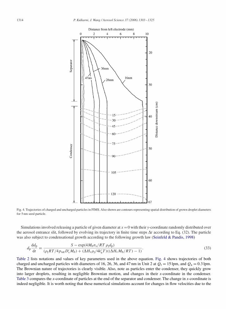
Fig. 4. Trajectories of charged and uncharged particles in FIMS. Also shown are contours representing spatial distribution of grown droplet diametersfor 5 nm seed particle.

Simulations involved releasing a particle of given diameter at x =0 with their y-coordinate randomly distributed overthe aerosol entrance slit, followed by evolving its trajectory in finite time steps t according to Eq. (32). The particlewas also subject to condensational growth according to the following growth law (Seinfeld & Pandis, 1998)

dpddp

dt= S − exp(4Mbs/RT ldp)

(lRT /4psatD′vMb) + (Hvl/4k′

aT )((HvMb/RT ) − 1). (33)

Table 2 lists notations and values of key parameters used in the above equation. Fig. 4 shows trajectories of bothcharged and uncharged particles with diameters of 16, 26, 36, and 47 nm in Unit 2 at Qt = 15 lpm, and Qa = 0.3 lpm.The Brownian nature of trajectories is clearly visible. Also, note as particles enter the condenser, they quickly growinto larger droplets, resulting in negligible Brownian motion, and changes in their x-coordinate in the condenser.Table 3 compares the x-coordinate of particles at the end of the separator and condenser. The change in x-coordinate isindeed negligible. It is worth noting that these numerical simulations account for changes in flow velocities due to the


Table 3Summary of particle transport and growth simulations

Diameter, dp (nm) x-coordinate of particle (mm)

ya = ls y = ls + lc

15 9.619 9.61218 6.488 6.46926 3.953 3.94836 2.795 2.80247 2.101 2.104

Results are averaged over 10 replicate simulations.aDistance from aerosol entrance.

non-uniform temperature profile in the condenser. The lower temperatures near the condenser walls lead to contractionof the flow, and the flow streamlines deviate outward at the entrance of the condenser. Such bending of flow streamlinesmay lead to a shift in particle position at the condenser exit with respect to its position at the separator exit. However,the simulations indicate that for the intended operating conditions of the instrument, any such effects originating fromtemperature gradient are negligible.

Fig. 4 also shows simulated trajectories of uncharged particles. Since uncharged particles do not experience anyelectrostatic force in the separator, their trajectories remain close to the ground electrode. Due to large residence timesthese particles also experience large diffusional spreading. However, their transport is still confined to a narrow regionnear the ground electrode, ensuring that they do not interfere with the measurement of charged particles.

Fig. 4 also shows the contour profiles of grown droplet diameters in the condenser. The growth calculations werebased on a particle with an initial diameter of 5 nm, following various particle trajectories in the condenser. Thecondensational growth is calculated using the flow, temperature, and saturation profiles obtained from FEM simulationsdescribed earlier. The calculations demonstrate that particles as small as 5 nm can be grown into optically detectabledroplets (> 120 m) using the proposed geometry and operating conditions.

4.4. Counting statistics of FIMS measurements

The improved time resolution of measurements often comes at the expense of reduction in counting statistics.The instrument design directly influences the counting statistics of size distribution measurements, and may limit themaximum frequency with which statistically significant measurements can be obtained. Counting statistics of FIMSmeasurements, using the proposed instrument geometry and flow conditions shown in Table 1, were investigated andare discussed below.

For each size bin, the uncertainty (c) of particle counts measured by FIMS can be approximated, based on Poissonstatistics, as c ≈ √

C, where C is the number of particle counts detected in the corresponding size bin. C can beestimated as

C = Qatc · N = Qatc ·(

dN

d ln dp

) (d ln dp

d ln Zp

) ln Zp, (34)

where tc is the sampling time, is the particle bipolar charging probability, and N is the particle number concentration.The signal-to-noise ratio is given by C/

√C = √

C. Assuming that the counts detected by each unit of FIMS aregrouped into 10 mobility size bins (evenly spaced on a logarithmic scale), and noting that each unit covers a factor of10 in mobility, we have ln Zp = (ln 10)/10. The counting statistics for measurement of typical remote continentaland marine aerosol (Seinfeld & Pandis, 1998) were calculated using Eq. (34), and the results are shown in Fig. 5.FIMS provides substantial improvements in measurement counting statistics over traditional SMPS. For typical remotecontinental aerosols, 1 s measurement time is sufficient to obtain excellent counting statistics. For clean marine aerosols,measurement time of 8 s reasonably captures the main characteristics of the aerosol size distribution. The countingstatistics of FIMS could be further improved by increasing the width b of the instrument channel and the aerosol flowrate.


dN/d

Log

10d p

(cm

-3)

0

2000

4000

6000

8000

10000

Remote continental aerosolSampling time= 1s

Diameter (nm)10 100 1000

dN/d

Log

10d p

(cm

-3)

0

50

100

150

200

250

300Marine aerosolSampling time

(a)

(b)

1s8s

Fig. 5. Calculated counting statistics of FIMS measurements of (a) a typical remote continental aerosol for a sampling time of 1 s and (b) a typicalmarine aerosol for a sampling time of 1 and 8 s.

5. Effect of particle diffusion on FIMS transfer function

Knowledge of FIMS transfer function (or probability density function) that accounts for all measurement uncertaintiesis necessary in order to accurately derive aerosol size distributions from FIMS measurements. For non-diffusingparticles, the uncertainty in measured mobility can be entirely attributed to finite stream width of aerosol flow. Thisuncertainty was discussed earlier, and the transfer function for a non-diffusing particle is given by Eq. (15). However,small particles with high diffusivity could further substantially increase the measurement uncertainties. Stolzenburg(1988) investigated the role of particle Brownian diffusion on the shape of DMA transfer function using an approachsimilar to that used by Tammet (1967) in his analysis of ion diffusion in aspiration condenser. More recently, Salm(2000) proposed a different approach to account for broadening of transfer function due to particle Brownian diffusionand/or turbulent diffusion. In this work we further extend the theoretical analysis developed earlier, which is similar tothat of Stolzenburg (1988), to take into account the effect of particle Brownian diffusion on the FIMS transfer functionP(Zp, out).

For a particle with mobility Zp, the transfer function is given by

P(Zp, out) =∫ 2,in

1,in

fe(in).ft−d(Zp, in, out) din, (35)

where the definition of fe(in) remains same as in Eq. (7). ft−d(Zp, in, out) is modified to include particle Browniandiffusion, and is given by (Stolzenburg, 1988)

ft−d(Zp, in, out) = 1√2

exp

[−1

2

(

)2]

, (36)


where , known as spread factor, is the standard deviation of . Calculation of spread factor will be discussed in detaillater. From the definition of given in Eq. (5), can be expressed as

= out − in = out − in − Zp. (37)

Combining Eq. (35)–(37), the probability density function P(Zp, out) for a diffusing particle can be expressed as

P(Zp, out) = 1

2,in − 1,in

∫ 2,in

1,in

1√2

exp

[−1

2

(out − in − Zp

)2]

din. (38)

After performing the integration, Eq. (38) becomes

P(Zp, out) = 1

2

1

2,in − 1,in

erf

(out − 1,in − Zp√

2

)− erf


2

), (39)

where the definition of error function has been used.However, it is more convenient to express the probability density function P(Zp, out) as a function of response

mobilityZ∗p , instead ofout. From the definition ofZ∗

p given in Eq. (13), it can be seen thatP(Zp, Z∗p)=P(Zp, out).

Then,

P(Zp, Z∗p) = 1

2

2,in − 1,in

erf


2

)− erf


2

)

= 1

2

2,in − 1,in

⎧⎪⎨⎪⎩erf

⎛⎜⎝ (Z∗p − Zp) + 2,in − 1,in

2√2

⎞⎟⎠−erf

⎛⎜⎝ (Z∗p − Zp) − 2,in − 1,in

2√2

⎞⎟⎠⎫⎪⎬⎪⎭ . (40)

It can be shown by inserting Eq. (26) into Eq. (40) that

P(Zp, Z∗p) = 1

2Z∗p

erf

((Z∗

p − Zp + 12Z∗

p)√2

)− erf

((Z∗

p − Zp − 12Z∗

p)√2

). (41)

The above equation is further non-dimensionalized using a normalized instrument response mobilityZ∗p , defined as

Z∗p = Z∗

p/Zp. Then,

P(Zp, Z∗p) = P(Zp, Z

∗p)

dZ∗p

dZ∗p

= 1

2Z∗p

erf

((Z∗

p − Zp + 12Z∗

p)√2

)− erf

((Z∗

p − Zp − 12Z∗

p)√2

)Zp

= 1

2Z∗p

erf

((Z∗

p − 1 + 12Z∗

p)

)− erf

((Z∗

p − 1 − 12Z∗

p)

), (42)

where Z∗p = Z∗

p/Zp and = √2/Zp.


From the definition of Z∗pmax

introduced earlier in Eq. (30), expression for P(Zp, Z∗p) can be further simplified to

P(Zp, Z∗p) = 1

2Z∗pmax

erf

((Z∗

p − 1 + 12Z∗

pmax)

)− erf

((Z∗

p − 1 − 12Z∗

pmax)

), (43)

Eq. (43) gives the probability density that a particle’s mobility Zp will be measured as normalized response mobilityZ∗

p . P(ZpZ∗p) reaches its maximum value at Z∗

p = 1 (i.e. when the response mobility Z∗p is same as particle mobility

Zp). In the non-diffusing limit as → 0, the first and second error function in Eq. (43) approach 1 and −1 respectively,and we have P(Zp, Z

∗p) → 1/Z∗

pmax.

Evaluation of P(Zp, Z∗p) requires knowledge of non-dimensional spread factor that characterizes the broadening of

the transfer function due to particle diffusion. An analytical expression for spread factor was obtained using analysissimilar to that used by Stolzenburg (1988), and is presented in Appendix A. The expression of is given by

2 = Pe−1

[2

(a

ls

)2

x∗ + 72(1 + )2Z2pmax

(x∗)]

, (44)

where Pe is the Peclet number defined as Pe = ZpExa/D = qV /kBT . Function (x∗) is given by

(x∗) =∫ x∗

0x2(1 − x)2 dx =

(x∗3

3− x∗4

2+ x∗5

5

), (45)

where x∗ is the location of centroid particle trajectory at the exit of the separator (normalized with respect to a). x∗ canbe obtained by solving Eq. (22) for given Z∗

p , Z∗pmax

, and . The transfer function P(Zp, Z∗p) can be calculated using

Eqs. (43)–(45).Fig. 6(a)–(c) show calculated transfer function P(Zp, Z

∗p) for particles of different sizes in Units 2, 3, and 4.

Also shown are the values of Z∗pmax

corresponding to each particle size in respective unit. The shape of the transferfunction varies considerably across different particle sizes and FIMS units. Since the transfer function is based on thenormalized instrument response mobility, the width of the distribution is a direct measure of the relative uncertainty inmeasured mobility; wider the distribution, larger the relative uncertainty. For a given FIMS unit, the transfer functionbecomes narrower for particles with smaller diameters, indicating lower relative uncertainties in measured mobility.This may seem counterintuitive at first, considering the fact that smaller particles have larger diffusivities. However, itcan be explained as follows. According to Eq. (43) width of the transfer function depends on two parameters Z∗

pmax

and . Z∗pmax

accounts for uncertainties due to finite stream width of aerosol flow, whereas takes into account thespreading of transfer function due to Brownian diffusion. According to Eq. (43), width of the transfer function decreaseswith decreasing Z∗

pmaxand . Though the absolute uncertainty Z∗

pmaxremains constant regardless of the particle size

(according to Eq. (27)), the relative uncertainty Z∗pmax

, however, decreases with increasing particle mobility (ordecreasing particle size). Similarly, non-dimensional spread factor also decreases with increasing particle mobility,even though the dimensional spread factor () increases with decreasing particle size. Increase in is only minorcompared to the increase in particle mobility Zp such that the net effect is decreasing with increasing Zp. Thus, lowervalues of Z∗

pmaxand for small particles result in narrower transfer functions.

Fig. 6 also shows the transfer functions of 15, 48, and 173 nm particles measured in Units 2, 3, and 4, respectively.These particles correspond to the smallest sizes (highest mobilities) measured in their respective units (Z∗

pmax= 1), and

have similar centroid particle trajectory. As shown in Fig. 6, the FIMS transfer function becomes broader as the particlesize decreases from 173 nm in Unit 4 to 15 nm in Unit 2. The spread factors () for 15, 48, and 173 nm particles are0.028, 0.009, and 0.003, respectively. For 15 nm particles in Unit 2, the transfer function exhibits substantial broadeningdue to Brownian diffusion. As Brownian diffusion becomes negligible for larger particles, the shape of the transferfunction resembles a box function as shown earlier for a case of non-diffusing particles (Fig. 2(b)–(c)).


P (Z

p, Z

p* /Zp)

0

5

10

15

20

dp*Zpmax

15 1 26 3.3 47 10

P (Z

p, Z

p* /Zp)

0

10

20

30

40

50

Zp*/Zp

0.8 0.9 1.0 1.1 1.2

P (Z

p, Z

p* /Zp)

0

10

20

30

40

50

60

Unit 2

Unit 3

Unit 4

dp*Zpmax

48 1 150 10

dp*Zpmax

173 1 585 5.4

(a)

(b)

(c)

~

~

~

Fig. 6. Transfer functions of representative particle diameters in Units 2, 3, and 4.

6. Comparison of FIMS and DMA

6.1. Comparison of transfer functions of FIMS and DMA

Fig. 7 shows comparison of transfer functions of TSI cylindrical DMA and the FIMS for non-diffusing particles.The non-diffusing DMA transfer function was calculated for aerosol and sheath flow of 1 and 10 lpm respectively,and equal aerosol and monodisperse flows. Transfer function of FIMS is based on a total flow rate of Qt = 9.7 lpmfor a 1m particle, with other parameters listed in Table 1. The shapes of the transfer function are quite different forthe two instruments. The DMA transfer function for non-diffusing particles is a triangle, whereas that of the FIMS is arectangle. Also, shown in the inset in Fig. 7 are idealized transfer functions for both instruments. The base width of thenon-diffusing DMA transfer function is 2DMA, with a height of unity. The width of the non-diffusing FIMS transfer

function is Z∗pmax

with height equal to1/(Z∗pmax

). For non-diffusing particles, the DMA transfer function remains

same for particles with different mobilities. In contrast however, the FIMS transfer function becomes narrower as Zpmax

decreases as discussed earlier (Fig. 6).


Zp /Z*pDMA

or Z*p /Zp

0.4 0.6 0.8 1.0 1.2

DM

A T

rans

fer

Func

tion,

Ω (

Z* p D

MA, Z

p/Z

* p DM

A)

0.0

0.2

0.4

0.6

0.8

1.0

1.2

FIM

S T

rans

fer

Func

tion,

P (

Zp,

Zp* /Z

p)

0

1

2

3

4

5

6

dp=1m(a)

Tra

nsfe

r Fu

nctio

n

1-βZ*

pmax

βZ*pmax

21-βDMA

1+βDMA1

1

1

~

1+βZ*

pmax

2

~

~

Fig. 7. Comparison of non-diffusing transfer functions of the TSI cylindrical DMA and the FIMS.

6 8 10 12 14

Res

olut

ion

(R)

1

10

100

15 20 25 30 35 40 45

(a) Unit 1 Unit 2

RnDMA

ndRFIMS

RDMA

dRFIMS

Diameter, dp (nm)200 400 600 800 1000

Diameter, dp (nm)60 80 100 120 140 160

Res

olut

ion

(R)

1

10

100

Unit 4 Unit 3

1.6 2.7 4.0 5.4 7.0 8.8 1.3 3.3 5.6 7.8 10.1

1.4 2.5 4.0 5.7 7.7

Z*pmax

1.0 1.8 2.7 3.9 5.2 6.7 8.4

~Z*

pmax

~

(b)

(d)(c)

Fig. 8. Mobility resolution of the FIMS over the particle size range of 5–1000 nm. Also shown are the resolutions of TSI cylindrical DMA andnano-DMA.


Table 4Mobility resolution of the particles measured by FIMS in Unit 2

dp (nm) → Resolution

15 (1)a 26 (2.9) 36 (5.5) 47 (9.1)

Flow Qt (lpm)

7 17.8 10.2 7.5 5.29 19.7 11.3 7.8 5.4

11 21.5 12.3 8.3 5.513 23.6 13.0 8.5 5.515 25.2 13.4 8.7 5.5

A constant Z∗pmax

of 9.75 × 10−7 m2 V−1 s−1 and = 0.02 were maintained at all flow rates.aNumbers in parenthesis indicate Z∗

pmaxfor each diameter.

6.2. Comparison of mobility resolution of FIMS and DMA

When particle Brownian diffusion is taken into account, the FIMS mobility resolution RdFIMS

(Zp

Z∗fwhh

)can be

calculated using Eq. (43). Fig. 8(a)–(d) show the resolution RdFIMS of all four FIMS units over the size range of

5 nm–1m. Also plotted in each figure is mobility resolution of non-diffusing particles (RndFIMS) based on Eq. (30).

For comparison, Fig. 8 also presents the mobility resolutions of TSI cylindrical DMA (RDMA) and TSI nano-DMA(RnDMA), that take into account particle diffusion. Resolutions of the two DMA were calculated using an aerosol flowrate of 1 lpm, and sheath flow rate of 10 lpm.

The resolution of FIMS for non-diffusing particles (RndFIMS) decreases with increasing diameter in each unit from about

50 at Z∗pmax

=1 to about 5 at Z∗pmax

=10 in each unit. This is characteristically different, and apparently counterintuitive,in comparison to the trend in the DMA resolution. For both cylindrical and nano DMAs, the resolution of non-diffusingparticles is constant, and is given by the reciprocal of aerosol-to-sheath flow rate ratio (1/DMA). Irrespective of particlesize, all (non-diffusing) particles have the same centroid particle streamline in DMA. Consequently, at a given aerosoland sheath flow rate, resolution of DMA remains constant. However in case of FIMS, since each particle follows adifferent trajectory, the ratio of aerosol flow to the total flow bounded by the particle trajectory at the separator exitis different. This can be further explained by transforming Eq. (30) using a position-dependent ratio of flow rates x ,defined as x = Qa/Q(x∗). Then, resolution R of FIMS for a non-diffusing particle can be written as

R = Zp

Z∗p

= Q(x∗) − (Qa/2)

Qa= 1 − 1

2x

x

1

x

. (46)

Thus analogous to the case of DMA, Eq. (46) shows that the mobility resolution of FIMS for non-diffusing particlesis given by the reciprocal of specific flow rate ratio x . Since x decreases with increasing x∗, the resolution increaseswith increasing particle mobility. Note that, for particle with maximum mobility (Z∗

pmax) measured by FIMS, Q(x∗) =

Qt, x = , and the resolution of the FIMS reaches its maximum value of 1/.Comparison of Rd

FIMS and RndFIMS in Units 1 and 2 clearly shows the degradation of FIMS resolution due to particle

diffusion. As particle diffusivity becomes negligible in Units 3 and 4, the resolution based on Eq. (43) is very closeto that given by Eq. (30). Mobility resolution of FIMS (Rd

FIMS) is higher than that of nano-DMA for particles smallerthan ∼ 12 nm(Z∗

pmax= 5.7) in Unit 1 and ∼ 35 nm(Zpmax = 5.21) in Unit 2. Rd

FIMS falls below that of DMA in Units 3

and 4 at Z∗pmax

greater than about 5. As discussed earlier in the design considerations, the operating conditions of FIMSare chosen assuming a minimum acceptable mobility resolution of 5. The mobility resolution of FIMS can be furtherimproved by reducing the flow rate ratio as shown in later discussions.

The influence of total flow rate Qt and flow rate ratio on the resolution of FIMS was also investigated. Table 4shows mobility resolution of FIMS (Rd

FIMS) at various total flow rates for a range of particle diameters. The voltageacross the electrodes in the separator was changed accordingly to maintain the same measurement range for each case.Particles with Z∗

pmaxcloser to unity (smaller particles) exhibit greater improvement in resolution with increasing Qt .


Table 5Mobility resolution of FIMS in Unit 2 at different values

Resolution

dp 15 nm 26 nm 36 nm 47 nmZ∗

pmax1 2.9 5.5 9.1

0.050 16.2 6.8 3.7 2.20.033 18.8 9.4 5.4 3.30.025 20.0 10.7 6.9 4.40.020 20.9 11.6 8.0 5.40.017 20.7 12.1 8.7 6.20.014 20.9 12.5 9.3 7.0

A constant Z∗pmax

of 9.75 × 10−7 m2 V−1 s−1 and Qt = 9.7 lpm were maintained at all flow rates.

Table 6Mobility resolution of FIMS in Unit 2 with different separator lengths (ls)

ls (cm) Resolution

dp 15 nm 26 nm 36 nm 47 nmZ∗

pmax1 2.9 5.5 9.1

5 36.7 16.5 9.2 5.610 28.2 14.3 9.0 5.615 23.6 13.0 8.5 5.520 20.9 11.6 8.0 5.4

A constant Z∗pmax

of 9.75 × 10−7 m2 V−1 s−1 and Qt = 9.7 lpm were maintained at all flow rates.

The resolution of 15 and 26 nm particles increased by 40% and 30% respectively, when the total flow rate is increasedfrom 7 to 15 lpm. In contrast, resolution of 47 nm particles increases only by 1.7%. Increasing Qt reduces the particleresidence time in the separator, which leads to smaller diffusional spreading of particles. Since the broadening oftransfer function due to particle diffusion is substantial for smaller particles with high diffusivity, increasing Qt willresult in greater improvements in mobility resolution for small particles. For larger particles however, the uncertaintyin measured mobility is mainly dictated by flow rate ratio . As a result, increasing Qt does not have a significanteffect on mobility resolution of larger particles. Table 5 shows FIMS resolution at various aerosol-to-sheath flow rateratios (). has a strong influence on the measurement resolution, especially for large particles. Resolution increasesby 29% for 15 nm particle, 83% for 26 nm, 150% for 36 nm, and 218% for 47 nm particle as is reduced from 0.05 to0.014. This clearly indicates that the mobility resolution of larger particles can be significantly improved by operatingthe instrument at lower .

While the degradation of resolution due to particle diffusion can be reduced by increasing the total flow rate Qt , ahigher total flow requires longer condenser to grow particles into detectable droplets, which may further lead to muchlonger condenser length. An alternative approach would be to reduce the length of the separator, similar to the designof the nano-DMA that increases the mobility resolution by reducing its column length. Table 6 shows the mobilityresolution for particles measured by Unit 2 with different separator lengths. Again, same measurement range wasmaintained for all cases by varying the separator voltage. As expected, reducing the separator length results in greaterimprovement in the resolution of smaller particles. Resolution of 15 nm particles increases from 20.9 to 36.7 whereasthe resolution of 47 nm particles only increases from 5.4 to 5.6.

The best mobility resolution can be achieved in each unit by using the shortest possible separator length. However,in the suggested FIMS configurations in Table 1 for Units 2–4, separator length was maintained constant for all units.Advantage of such a design is that a single unit can be interchangeably used as Units 2–4 by simply changing theseparator voltage.


7. Summary and conclusions

A novel Fast Integrated Mobility Spectrometer (FIMS) is described for characterizing aerosol size distributions withhigh-time and size resolution, and excellent counting statistics. FIMS combines electrical mobility-based classificationand particle counting in a single unit, and eliminates the need for voltage scanning required in traditional scanningDifferential Mobility Analyzer (DMA) techniques. As a result, aerosol size distributions can be obtained at sub-secondtime intervals.

A theoretical framework has been developed to obtain the transfer function of a single FIMS, unit accounting foruncertainties originating from particle Brownian diffusion, and finite stream width of aerosol flow. The FIMS transferfunction was used to characterize measurement resolution of the instrument over a wide range of operating conditions.Results show that a decade of mobility can be measured in a single FIMS unit with a minimum mobility resolutionof 5. The mobility resolution of a single FIMS unit increases with decreasing particle size, which is attributed to thehigher specific flow rate ratios for smaller particles. Compared to conventional cylindrical DMA operated under typicaloperating conditions, the resolution of FIMS is much higher for smaller particles, and is comparable to that of DMA forlarger particles. The counting statistics of FIMS measurements were also investigated. It was shown that for a typicalremote continental aerosol, 1 s measurement time provides excellent signal-to-noise ratio.

Detailed numerical simulations were also carried out to study the particle transport and growth kinetics in FIMS.Results indicate excellent activation efficiencies for particles larger than 5 nm. Particles as small as 5 nm can be growninto droplets larger than 120 m to facilitate their reliable optical detection.

Acknowledgments

This work was supported by the Office of Biological and Environmental Research, Department of Energy, underContract DE-AC02-98CH10866, the Office of Global Programs of National Oceanic and Atmospheric Administrationunder Contract NRMT0000-5-203, and the Laboratory Directed Research and Development program at the BrookhavenNational Laboratory. Stimulating discussions with Dr. Peter Takacs, Dr. Peter Daum, and Dr. Stephen Springston aregratefully acknowledged. Jian Wang also acknowledges partial support from the Goldhaber Distinguished Fellowshipfrom Brookhaven Science Associates.

Appendix A

This appendix describes the derivation of spread factor required to evaluate P(Zp, Z∗p) in Eq. (43). Similar to the

work of Stolzenburg (1988), a few approximations were made in the derivation of the spread factor. It was assumed thatonly diffusion in the direction orthogonal to the particle stream function (cross-stream direction denoted by ; see Fig.2) was significant, and streamwise (s-direction) diffusion was negligible. Particle losses to the walls of the separatorwere also neglected. The root-mean-square displacement of particles from the centroid particle trajectory is a functionof time according to Einstein equation (Fuchs, 1964)

d〈 2〉 = 2D dt . (47)

The distribution of particles is Gaussian with variance 2 = 〈 2〉. can be related to r by (Stolzenburg, 1988)

=(

) . (48)

With = 0 on the particle stream line , the variation of with can be approximated by the Taylor series expansion(Stolzenburg, 1988):

( , s)| =0 +

∣∣∣∣ =0

. (49)


Let r represent the particle position vector, at = 0, both r/ and ∇ are perpendicular to the particle streamlineand we have

∣∣∣∣r

∣∣∣∣ .|∇| = (1).

√v2x + v2

y = v, (50)

where v is the magnitude of particle velocity. Combining Eqs. (48) and (50), we have

= v . (51)

Since the particle diffusivity D is constant, total diffusional spreading can then be calculated by integrating over thepath of the trajectory (Stolzenburg, 1988):

2 =

∫ exit

entranced2

=∫ exit

entranced(v2

) =∫ exit

entrancev2 d(2

) = 2D

∫ exit

entrancev2 dt . (52)

The particle velocity is given by

v2 = v2x + v2

y = u2y(x) + (ZpEx)

2, (53)

where uy(x) can be evaluated using Eq. (20). Inserting Eq. (53) into Eq. (52), we have

2 = 2D

∫ exit

entrance

[(6Qt

ab[x(1 − x)]

)2

+ (ZpEx)2

]dt . (54)

Noting x = (vxt)/a = (ZpExt)/a, we can change the integration variable t in Eq. (54) to x:

2 = 22

(Zp)2 = 4D

(Zp)2

∫ x∗

0

[(6Qt

ab[x(1 − x)]

)2

+ (ZpEx)2

] (a

ZpEx

)dx, (55)

where x∗ is the location of the particle centroid trajectory at the separator exit. After carrying out the integration, wecan simplify the above equation to

2 = Pe−1

[2

(a

ls

)2

x∗ + 72(1 + )2Z2pmax

(x∗)]

, (56)

where Pe is the Peclet number defined as Pe = ZpEya/D = qV /kBT , q is the total electric charge on the aerosolparticle, kB is Boltzmann’s constant, and T is the temperature. Function (x∗) is given by

(x∗) =∫ x∗

0x2(1 − x)2 dx =

(x∗3

3− x∗4

2+ x∗5

5

), (57)

where x∗ can be obtained by solving Eq. (22) for given Z∗p , Z∗

pmax, and .

References

Bird, R. B., Stewart, W. E., & Lightfoot, E. N. (1960). Transport phenomena. New York: Wiley.Brock, C. A., Schröder, F., Kärcher, B., Petzold, A., Rusen, R., & Fiegbig, M. (2000). Ultrafine particle size distributions measured in aircraft exhaust

plumes. Journal of Geophysical Research, 105, 26,555–26,567.Ermak, D. L. (1975). Computer simulation of charged particles in solution. I: technique and equilibrium properties. Journal of Chemical Physics,

62, 4189–4196.Flagan, R. C. (1998). History of electrical aerosol measurements. Aerosol Science and Technology, 28(4), 301–380.Flagan, R. C. (1999). On differential mobility analyzer resolution. Aerosol Science and Technology, 30(6), 556–570.Fuchs, N. A. (1964). The mechanics of aerosols. Oxford: Pergamon Press.Hering, S. V., & McMurry, P. H. (1991). Optical counter response to monodisperse atmospheric aerosols. Atmospheric Environment Part A, 25(2),

463–468.


Johnson, T., Caldow, R., Pocher, A., Mirme, A., & Kittelson, D. (2004). A new electrical mobility particle sizer spectrometer for engine exhaustparticle measurements. SAE 2004 World congress & exhibition SAE-2004-01-134, Detroit, MI.

Knutson, E. O., & Whitby, K. T. (1975). Aerosol classification by electric mobility: Apparatus, theory, and applications. Journal of Aerosol Science,6, 443–451.

Mirme, A. (1994). Electrical aerosol spectrometry. Ph.D. Thesis, Universitatis Tartuensis, Tartu, Estonia.Mirme, A., Noppel, M., Peil, I., Salm, J., Tamm, E., Tammet, H., 1984. Multi-channel electric aerosol spectrometer. In 11th international conference

on atmospheric aerosols, condensation and ice nuclei, Budapest (Vol. 2, pp. 155–159).Russell, L. M., Flagan, R. C., & Seinfeld, J. H. (1995). Asymmetric instrument response resulting from mixing effects in accelerated DMA-CPC

measurements. Aerosol Science and Technology, 23, 491–509.Salm, J. (2000). Diffusion distortions in a differential mobility analyzer: The shape of apparent mobility spectrum. Aerosol Science and Technology,

32(6), 602–612.Seinfeld, J. H., & Pandis, S. N. (1998). Atmospheric chemistry and physics. New York: Wiley.Stolzenburg, M. (1988). An ultrafine aerosol size distribution measuring system. Ph.D. thesis, St. Paul, University of Minnesota.Tammet, H. (1967). Aspiration method for the determination of atmospheric ion spectra, (Vol II). Jerusalem: Israel program for scientific translations.Tammet, H., Mirme, A., & Tamm, E. (1998). Electrical aerosol spectrometer of Tartu University. Journal of Aerosol Science, 29, S427–S428.Tammet, H., Mirme, A., & Tamm, E. (2002). Electrical aerosol spectrometer of Tartu University. Atmospheric Research, 62, 315–324.Wang, S. C., & Flagan, R. C. (1989). Scanning electrical mobility spectrometer. Journal of Aerosol Science, 20, 1485–1488.Wang, J., McNeill, V. F., Collins, D. R., & Flagan, R. C. (2002). Fast mixing condensation nucleus counter: Application to rapid scanning differential

mobility analyzer measurements. Aerosol Science and Technology, 36(6), 678–689.

new fast integrated mobility spectrometer for real-time measurement of aerosol size...

Documents