new government polytechnic college, patna -13 lab …

NEW GOVERNMENT POLYTECHNIC

COLLEGE, PATNA -13

LAB MANUAL

HYDRAULICS LAB

DEPARTMENT OF CIVIL ENGINEERING

Name :

Branch :

Roll No. :

Group :

EXPERIMENT: - 1 VERIFICATION OF BERNOULLI’S THEORM

OBJECTIVE:- To verify the Bernoulli’s theorem experimentally.

SAFETY PRECAUTIONS:-

• Apparatus should be in leveled condition.

• Reading must be taken in steady or nearby steady conditions and it should be noted that water level in

the inlet supply tank should reach the overflow condition.

• There should not be any air bubble in the piezometer and in the Perspex duct.

• By closing the regulating valve, open the control valve slightly such that the water level in the inlet

supply tank reaches the overflow conditions. At this stage check that pressure head in each piezometer

tube is equal. If not adjust the piezometer to bring it equal.

•

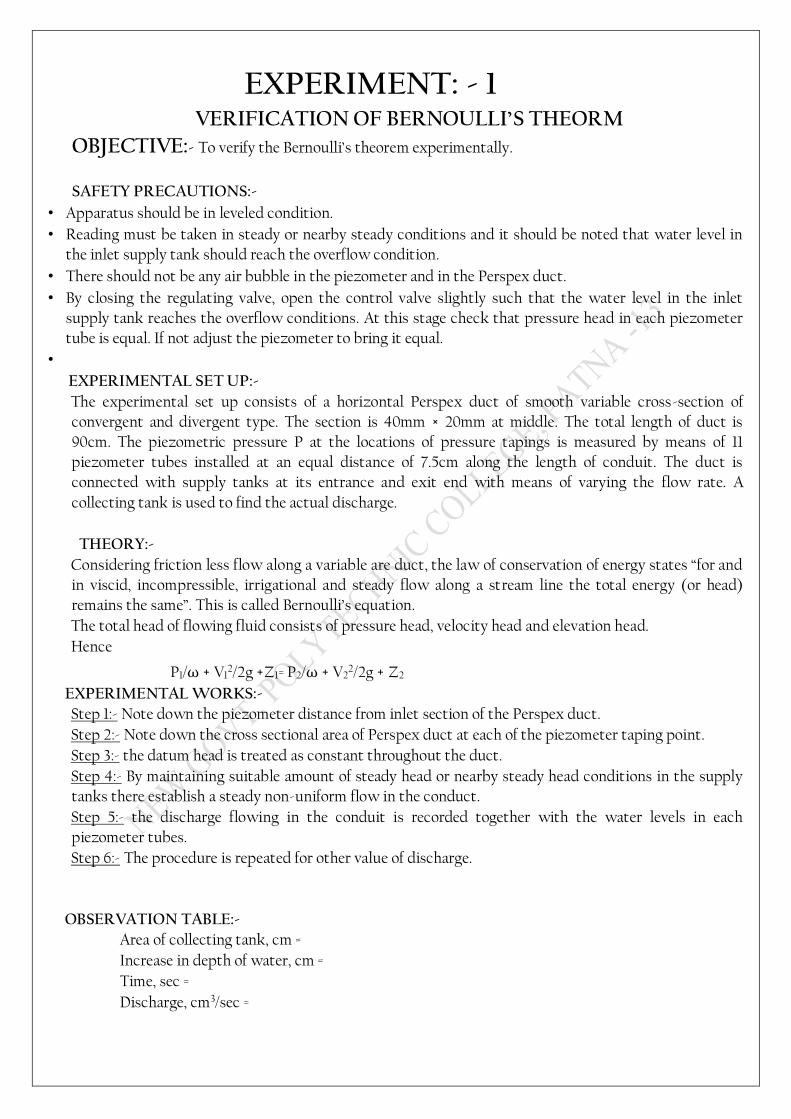
EXPERIMENTAL SET UP:-

The experimental set up consists of a horizontal Perspex duct of smooth variable cross-section of

convergent and divergent type. The section is 40mm × 20mm at middle. The total length of duct is

90cm. The piezometric pressure P at the locations of pressure tapings is measured by means of 11

piezometer tubes installed at an equal distance of 7.5cm along the length of conduit. The duct is

connected with supply tanks at its entrance and exit end with means of varying the flow rate. A

collecting tank is used to find the actual discharge.

THEORY:-

Considering friction less flow along a variable are duct, the law of conservation of energy states “for and

in viscid, incompressible, irrigational and steady flow along a stream line the total energy (or head)

remains the same”. This is called Bernoulli’s equation.

The total head of flowing fluid consists of pressure head, velocity head and elevation head.

Hence

P1/ω + V12/2g +Z1= P2/ω + V2

2/2g + Z2

EXPERIMENTAL WORKS:-

Step 1:- Note down the piezometer distance from inlet section of the Perspex duct.

Step 2:- Note down the cross sectional area of Perspex duct at each of the piezometer taping point.

Step 3:- the datum head is treated as constant throughout the duct.

Step 4:- By maintaining suitable amount of steady head or nearby steady head conditions in the supply

tanks there establish a steady non-uniform flow in the conduct.

Step 5:- the discharge flowing in the conduit is recorded together with the water levels in each

piezometer tubes.

Step 6:- The procedure is repeated for other value of discharge.

OBSERVATION TABLE:-

Area of collecting tank, cm =

Increase in depth of water, cm =

Time, sec =

Discharge, cm3/sec =

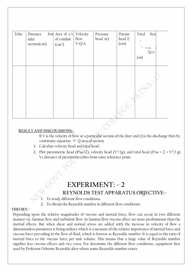
Tube Distance from

inlet section(cm)

Area of c/s

of conduit

(cm2)

Velocity flow V=Q/A

Pressure head m)

Datum head Z (cm)

Total head

2 /2g+z

(cm)

RESULT AND DISCOUSSIONS:-

If V is the velocity of flow at a particular section of the duct and Q is the discharge then by

continuity equation: V= Q/area of section

1. Calculate velocity head and total head..

2. Plot piezometric head (P/ω+Z), velocity head (V2/2g), and total head (P/ω + Z + V2/2 g)

Vs distance of piezometer tubes from same reference point.

EXPERIMENT: - 2 REYNOLDS TEST APPARATUS OBJECTIVE:-

1. To study different flow conditions.

2. To obtain the Reynolds number in different flow conditions.

THEORY:-

Depending upon the relative magnitudes of viscous and inertial force, flow can occur in two different

manner viz. laminar flow and turbulent flow. In laminar flow viscous effect are more predominant than the

inertial effects. But when shear and normal stress are added with the increase in velocity of flow a

dimensionless parameter is being utilizes which is a measure of the relative importance of inertial force and

viscous force prevailing in the flow of fluid, which is known as Reynolds number. It is equal to the ratio of

inertial force to the viscous force per unit volume. This means that a large value of Reynolds number

signifies less viscous effects and vice versa. For determine the different flow conditions, equipment first

used by Professor Osborne Reynolds after whose name Reynolds number exists.

The motion is laminar or turbulent according as the value of Re is less than or greater than a certain value.

If a liquid such as water is allowed to flow through a glass tubes, and if one of the liquid filament is made

visible by means of dye, then by watching this filament we may get insight into the actual behavior of the

liquid as it moves along. After the water in the supply tank has stood for several hours to allow it to come

completely to rest. The outlet valve is slightly opened. The central thread of dye carried along by the slow

stream of in the glass tube is seen to be nearly as steady and well defined as the indicating column in an

alcohol thermometer. But when, as a result of further opening of valve, the water velocity passes a specific

limit, a change occurs, the rigid thread of dye begins to break up and to group momentarily ill- defined. The

moment the dye deviated from its straight line pattern corresponds to the condition when the flow in the

conduit is no longer in laminar conditions. The discharge, Q flowing in the conduit at this moment is

measured and the Reynolds number 4Q/πdν (in which d is the diameter of the conduit and ν is the

kinematics viscosity of water is computed. This is the lower critical Reynolds number. Finally, at high

velocities the dye mixes completely with the water and the colored mixture fills the tube.

EXPERIMENTAL SET UP:-

Apparatus consist of storage cum supply tank, which has the provision for supplying colored dye through

jet. A Perspex tube is provided to visualize the different flow condition. The entry of water in Perspex tube

is through elliptical bell mouth to have smooth flow at the entry. A regulating valve is provided on the

downstream side of the tube to regulate the flow. The discharge must be varied very gradually from a

smaller to larger value. A collecting tank is used to find the actual discharge through the Perspex tube.

EXPERIMENTAL WORK:-

Step 1:- Note down the relevant dimensions as diameter of Perspex tube, area of collecting tank, room

temperature etc.

Step 2:- by maintaining suitable amount of steady flow in the Perspex tube, open inlet of the dye tank so

that the dye stream moves as a straight line in the tube.

Step 3:- the discharge flowing in the Perspex tube is recorded.

Step 4:- this procedure is repeated for other values of discharge.

Step 5:- by increasing the velocity of flow in the Perspex tube, again open the inlet of the dye tank so that

the dye stream begins to break up in the tube, which shows the fluid is no more in the laminar conditions.

Hence transition stage occurs.

Step 6:- this discharge flowing in the Perspex tube is recorded.


Step 8:- on further increase in the velocity of flow in the Perspex tube, again open the inlet of dye tank so

that the dye mixes completely in the tube which shows fluid is no more in the transition stage. Hence

turbulent flow occurs in the tube.

Step 9:- the discharge flowing in the Perspex tube is recorded.


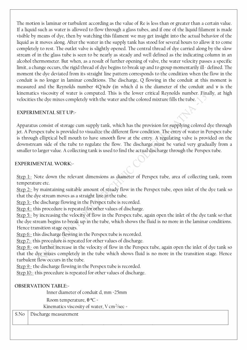
OBSERVATION TABLE:-

Inner diameter of conduit d, mm =25mm

Room temperature, θ ⁰C =

Kinematics viscosity of water, V cm2/sec =

S.No Discharge measurement

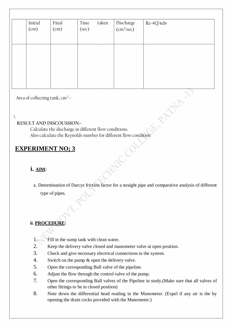
Initial

(cm)

Final

(cm)

Time

(sec)

taken Discharge

(cm3/sec)

Re=4Q/πdν

Area of collecting tank, cm2 =

\

RESULT AND DISCOUSSION:-

Calculate the discharge in different flow conditions.

Also calculate the Reynolds number for different flow condition

EXPERIMENT NO; 3

i. AIM:

a. Determination of Darcys friction factor for a straight pipe and comparative analysis of different

type of pipes.

ii. PROCEDURE:

1. Fill in the sump tank with clean water.

2. Keep the delivery valve closed and manometer valve at open position.

3. Check and give necessary electrical connections to the system.

4. Switch on the pump & open the delivery valve.

5. Open the corresponding Ball valve of the pipeline.

6. Adjust the flow through the control valve of the pump.

7. Open the corresponding Ball valves of the Pipeline in study.(Make sure that all valves of

other fittings to be in closed position)

8. Note down the differential head reading in the Manometer. (Expel if any air is the by

opening the drain cocks provided with the Manometer.)

9. Operate the Butterfly valve to note down the collecting tank reading against the known

time and keep it open when the readings are not taken.

10. Change the flow rate and repeat the experiment.

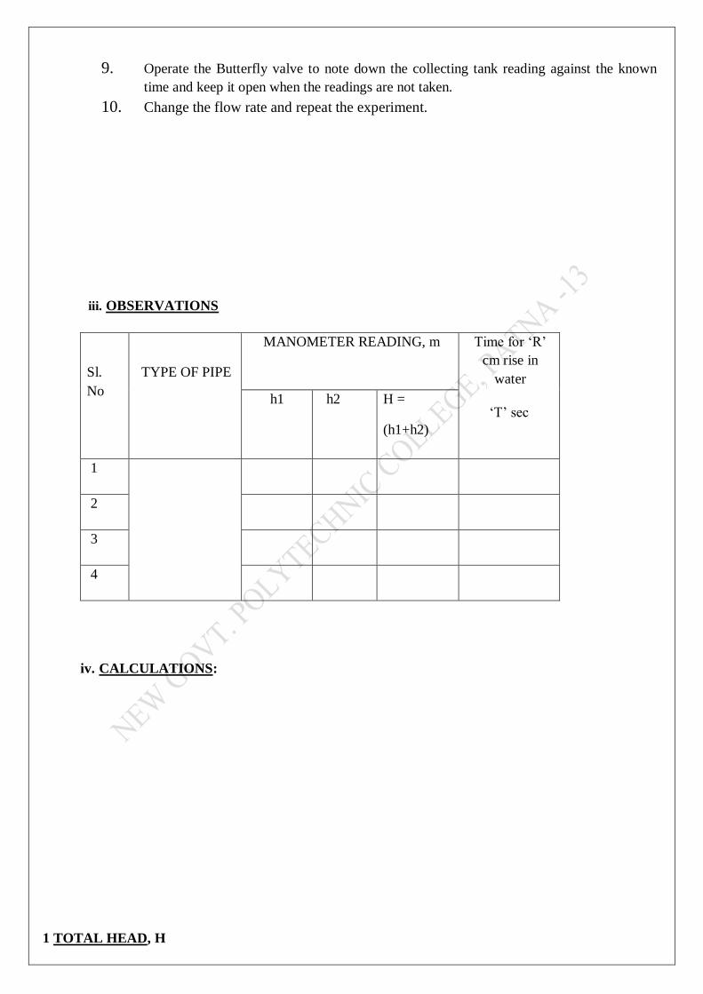
iii. OBSERVATIONS

Sl.

No

TYPE OF PIPE

MANOMETER READING, m Time for ‘R’

cm rise in

water

‘T’ sec h1 h2 H =

(h1+h2)

1

2

3

4

iv. CALCULATIONS:

1 TOTAL HEAD, H

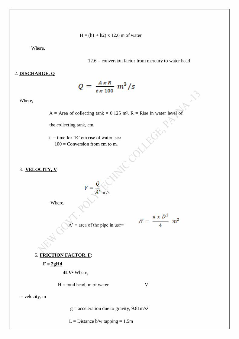
H = (h1 + h2) x 12.6 m of water

Where,

12.6 = conversion factor from mercury to water head

2. DISCHARGE, Q

Where,

A = Area of collecting tank = 0.125 m². R = Rise in water level of

the collecting tank, cm.

t = time for ‘R’ cm rise of water, sec

100 = Conversion from cm to m.

3. VELOCITY, V

m/s

Where,

A’ = area of the pipe in use=

5. FRICTION FACTOR, F:

F = 2gHd

4LV² Where,

H = total head, m of water V

= velocity, m

g = acceleration due to gravity, 9.81m/s²

L = Distance b/w tapping = 1.5m

d= Dia of pipe

v. RESULTS:

FRICTION FACTOR, F for :

a. 1" G.I =

b. 3/4" G.I =

c. 1/2" G.I =

1" PVC =

EXPERIMENT NO-4

. MINOR LOSSES IN PIPES

OBJECTIVES:

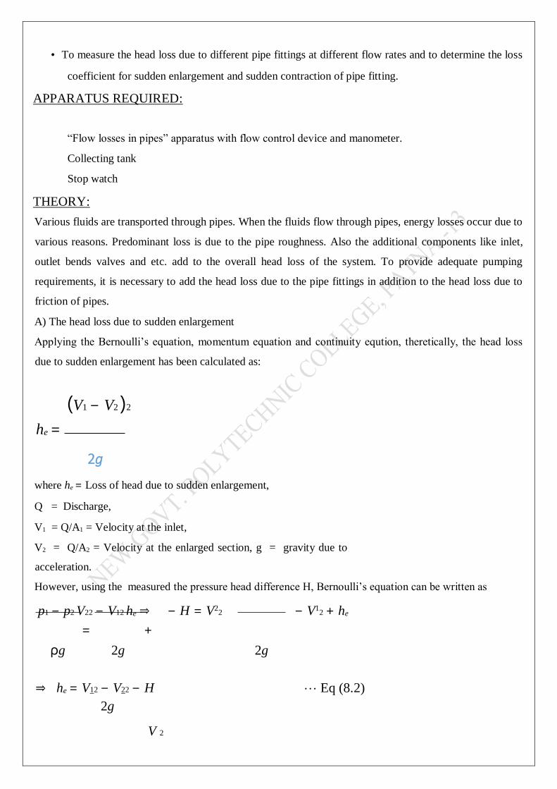
• To measure the head loss due to different pipe fittings at different flow rates and to determine the loss

coefficient for sudden enlargement and sudden contraction of pipe fitting.

APPARATUS REQUIRED:

“Flow losses in pipes” apparatus with flow control device and manometer.

Collecting tank

Stop watch

THEORY:

Various fluids are transported through pipes. When the fluids flow through pipes, energy losses occur due to

various reasons. Predominant loss is due to the pipe roughness. Also the additional components like inlet,

outlet bends valves and etc. add to the overall head loss of the system. To provide adequate pumping

requirements, it is necessary to add the head loss due to the pipe fittings in addition to the head loss due to

friction of pipes.

A) The head loss due to sudden enlargement

Applying the Bernoulli’s equation, momentum equation and continuity eqution, theretically, the head loss

due to sudden enlargement has been calculated as:

(V1 − V2 )2

he =

2g

where he = Loss of head due to sudden enlargement,

Q = Discharge,

V1 = Q/A1 = Velocity at the inlet,

V2 = Q/A2 = Velocity at the enlarged section, g = gravity due to

acceleration.

However, using the measured the pressure head difference H, Bernoulli’s equation can be written as

p1 − p2 V22 − V12 he ⇒ − H = V22 − V1

2 + he

= +

ρg 2g 2g

⇒ he = V12 − V22 − H Eq (8.2)

2g

V 2

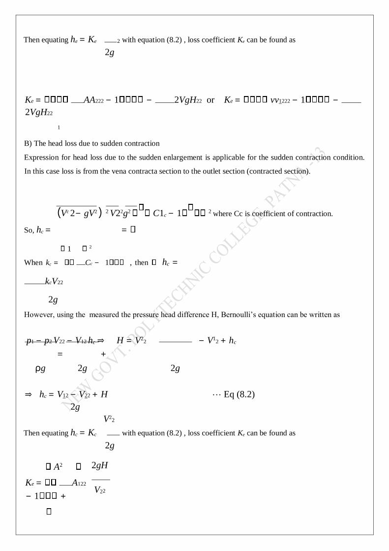
Then equating he = Ke 2 with equation (8.2) , loss coefficient Ke can be found as

2g

Ke = AA222 − 1 − 2VgH22 or Ke = vv1222 − 1 −

2VgH22

1

B) The head loss due to sudden contraction

Expression for head loss due to the sudden enlargement is applicable for the sudden contraction condition.

In this case loss is from the vena contracta section to the outlet section (contracted section).

(Vc 2− gV2 ) 2 V22g2 C1c − 1 2 where Cc is coefficient of contraction.

So, hc = =

1 2

When kc = Cc − 1 , then hc =

kcV22

2g

However, using the measured the pressure head difference H, Bernoulli’s equation can be written as

p1 − p2 V22 − V12 hc ⇒ H = V22 − V1

2 + hc

= +

ρg 2g 2g

⇒ hc = V12 − V22 + H Eq (8.2)

2g

V22

Then equating hc = Kc with equation (8.2) , loss coefficient Ke can be found as

2g

A2

Ke = A122

− 1 +

2gH

V22

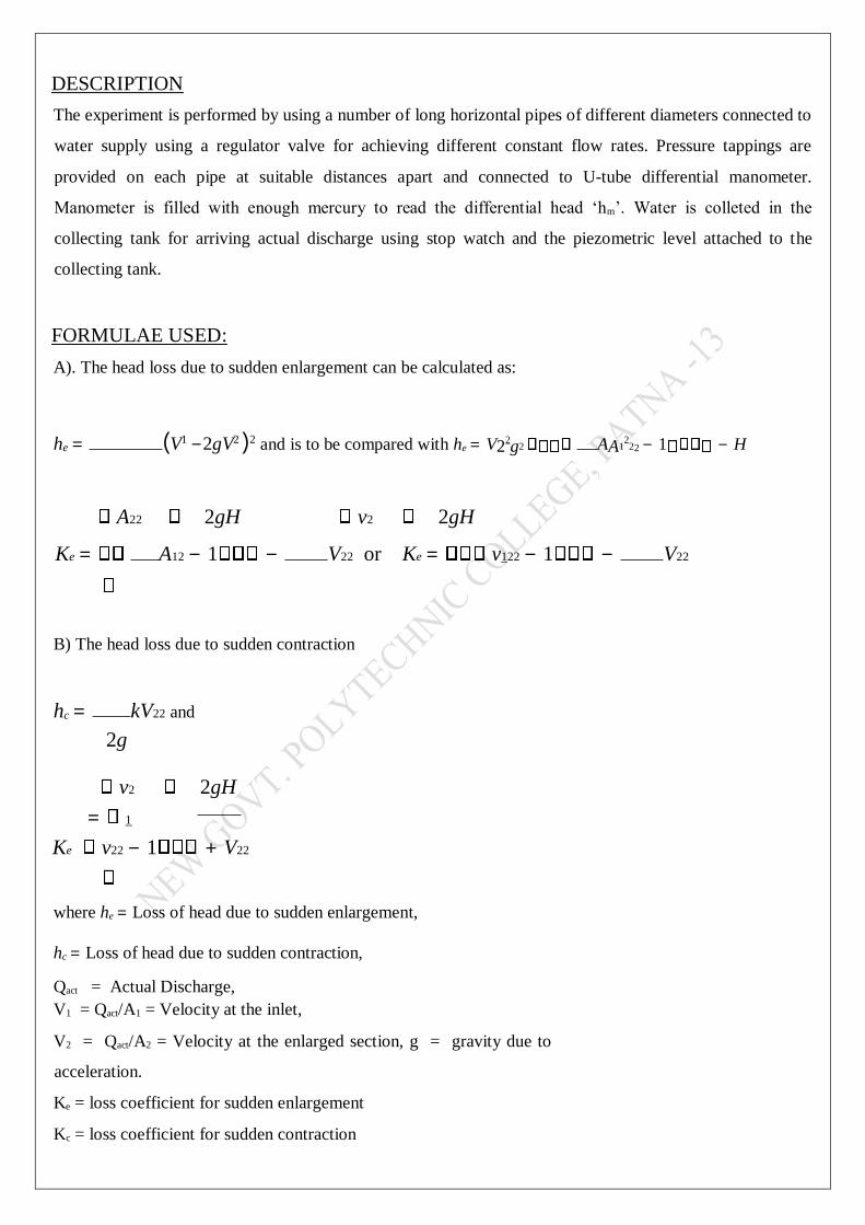
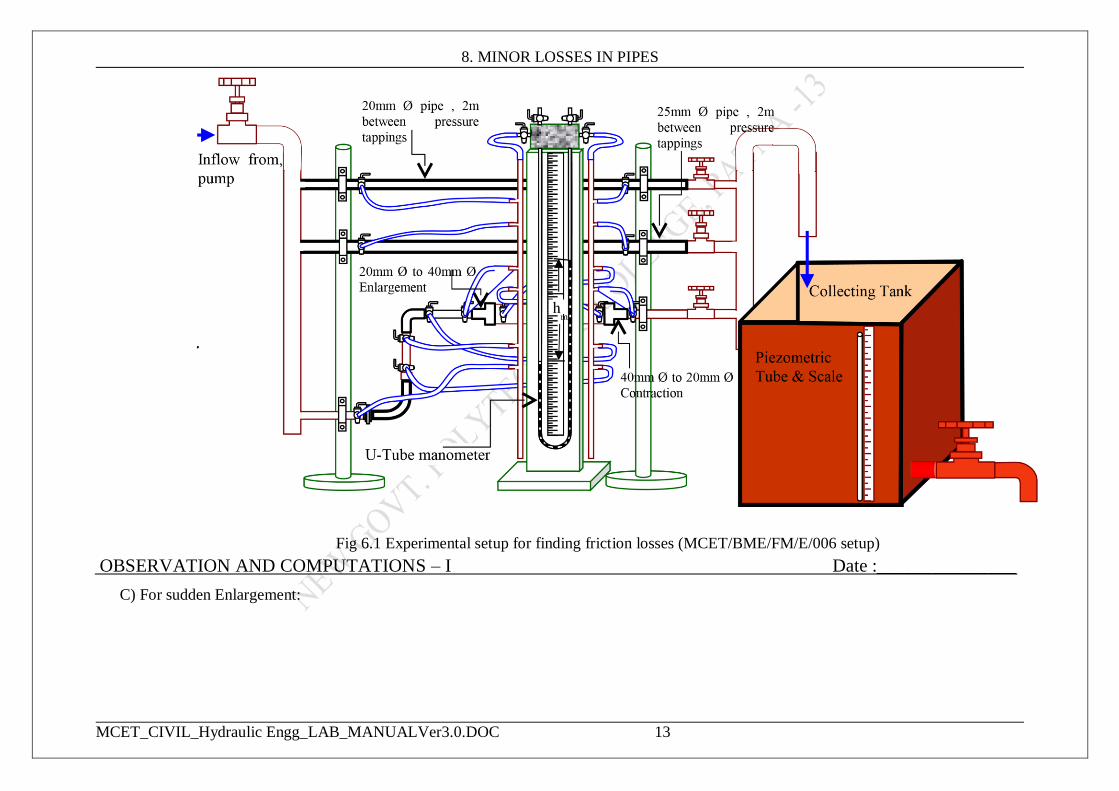
DESCRIPTION

The experiment is performed by using a number of long horizontal pipes of different diameters connected to

water supply using a regulator valve for achieving different constant flow rates. Pressure tappings are

provided on each pipe at suitable distances apart and connected to U-tube differential manometer.

Manometer is filled with enough mercury to read the differential head ‘hm’. Water is colleted in the

collecting tank for arriving actual discharge using stop watch and the piezometric level attached to the

collecting tank.

FORMULAE USED:

A). The head loss due to sudden enlargement can be calculated as:

he = (V1 −2gV2 )2 and is to be compared with he = V22g2 AA1

222 − 1 − H

A22 2gH v2 2gH

Ke = A12 − 1 − V22 or Ke = v122 − 1 − V22

B) The head loss due to sudden contraction

hc = kV22 and

2g

v2 2gH

= 1

Ke v22 − 1 + V22

where he = Loss of head due to sudden enlargement,

hc = Loss of head due to sudden contraction,

Qact = Actual Discharge,

V1 = Qact/A1 = Velocity at the inlet,

V2 = Qact/A2 = Velocity at the enlarged section, g = gravity due to

acceleration.

Ke = loss coefficient for sudden enlargement

Kc = loss coefficient for sudden contraction

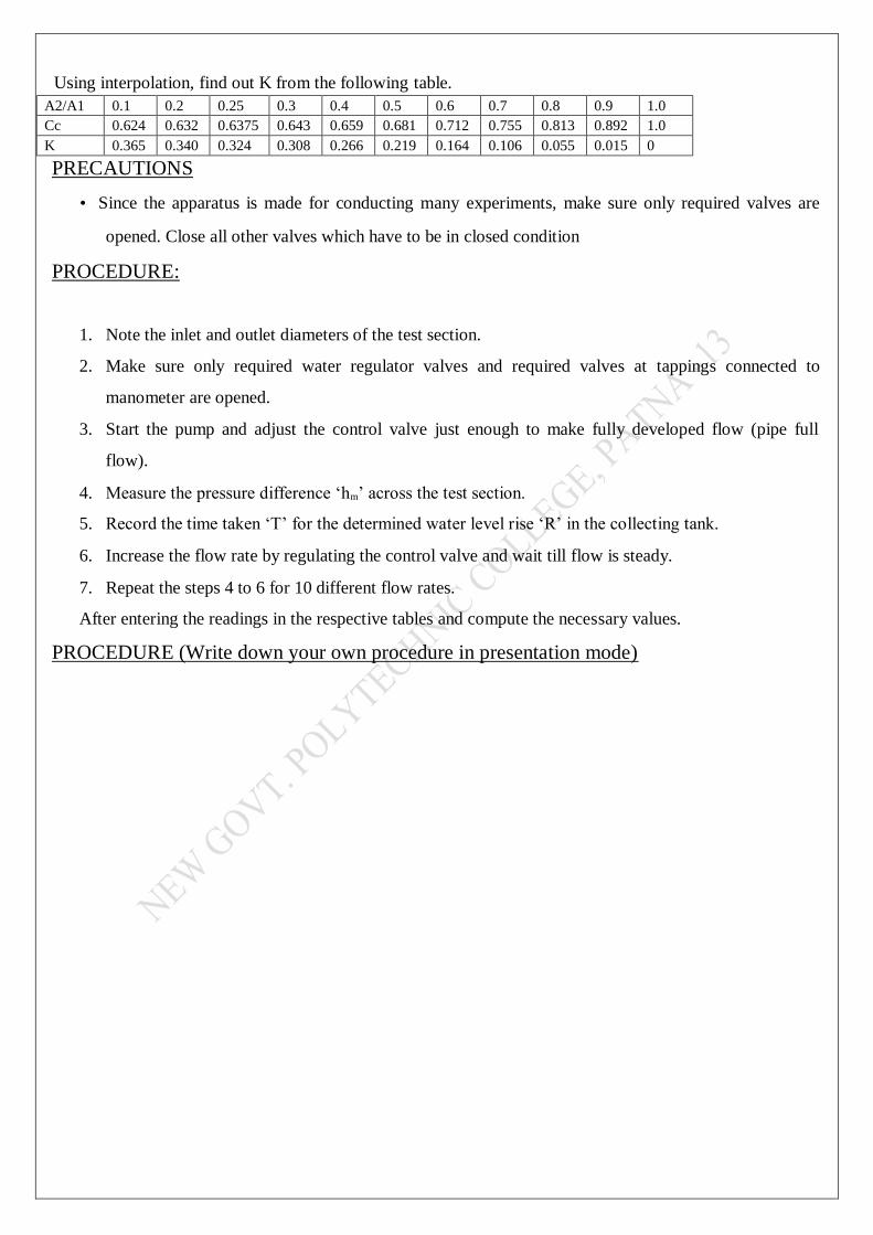
Using interpolation, find out K from the following table.

A2/A1 0.1 0.2 0.25 0.3 0.4 0.5 0.6 0.7 0.8 0.9 1.0 Cc 0.624 0.632 0.6375 0.643 0.659 0.681 0.712 0.755 0.813 0.892 1.0

K 0.365 0.340 0.324 0.308 0.266 0.219 0.164 0.106 0.055 0.015 0

PRECAUTIONS

• Since the apparatus is made for conducting many experiments, make sure only required valves are

opened. Close all other valves which have to be in closed condition

PROCEDURE:

1. Note the inlet and outlet diameters of the test section.

2. Make sure only required water regulator valves and required valves at tappings connected to

manometer are opened.

3. Start the pump and adjust the control valve just enough to make fully developed flow (pipe full

flow).

4. Measure the pressure difference ‘hm’ across the test section.

5. Record the time taken ‘T’ for the determined water level rise ‘R’ in the collecting tank.

6. Increase the flow rate by regulating the control valve and wait till flow is steady.

7. Repeat the steps 4 to 6 for 10 different flow rates.

After entering the readings in the respective tables and compute the necessary values.

PROCEDURE (Write down your own procedure in presentation mode)

8. MINOR LOSSES IN PIPES

MCET_CIVIL_Hydraulic Engg_LAB_MANUALVer3.0.DOC 13

Fig 6.1 Experimental setup for finding friction losses (MCET/BME/FM/E/006 setup)

OBSERVATION AND COMPUTATIONS – I Date :_______________

C) For sudden Enlargement:



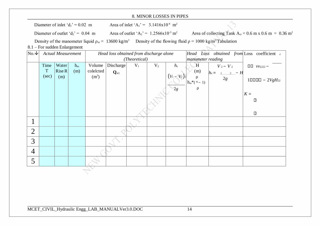
Diameter of inlet ‘d1’ = 0.02 m Area of inlet ‘A1’ = 3.1416x10-4 m2

Diameter of outlet ‘d2’ = 0.04 m Area of outlet ‘A2’ = 1.2566x10-3 m2 Area of collecting Tank Act = 0.6 m x 0.6 m = 0.36 m2

Density of the manometer liquid ρm = 13600 kg/m3 Density of the flowing fluid ρ = 1000 kg/m3 Tabulation

8.1 – For sudden Enlargement

No. Actual Measurement Head loss obtained from discharge alone

(Theoretical)

Head Loss obtained from

manometer reading

Loss coefficient e

vv1222 −

1 − 2VgH22

K =

Time

T

(sec)

Water

Rise R

(m)

hm

(m)

Volume

colelcted

(m3)

Discharge

Qact

V1 V2 he

(V1 − V2 )2

2g

H

(m)

ρ

hm*( m − 1)

ρ

V 2 − V 2

he = 1 2 − H

2g

1

2

3

4

5



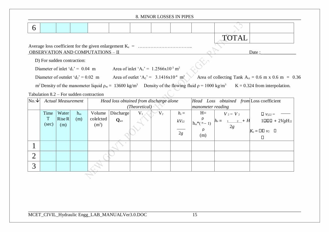
6

TOTAL

Average loss coefficient for the given enlargement Ke = ……………………………..

OBSERVATION AND COMPUTATIONS – II Date :_______________

D) For sudden contraction:

Diameter of inlet ‘d1’ = 0.04 m Area of inlet ‘A1’ = 1.2566x10-3 m2

Diameter of outnlet ‘d2’ = 0.02 m Area of outlet ‘A2’ = 3.1416x10-4 m2 Area of collecting Tank Act = 0.6 m x 0.6 m = 0.36

m2 Density of the manometer liquid ρm = 13600 kg/m3 Density of the flowing fluid ρ = 1000 kg/m3 K = 0.324 from interpolation.

Tabulation 8.2 – For sudden contraction

No. Actual Measurement Head loss obtained from discharge alone

(Theoretical)

Head Loss obtained from

manometer reading

Loss coefficient

v122 −

1 + 2VgH22

Ke = v2

Time

T

(sec)

Water

Rise R

(m)

hm

(m)

Volume

colelcted

(m3)

Discharge

Qact

V1 V2 hc =

kV22

2g

H= ρ

hm*( m − 1)

ρ

(m)

V 2 − V 2

he = 1 2 + H

2g

1

2

3



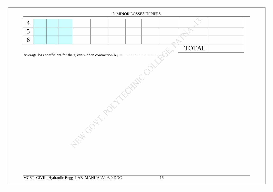
4

5

6

TOTAL

Average loss coefficient for the given sudden contraction Kc = ……………………………..


GRAPH:

1) Head loss he vs. Actual discharge Qact for sudden enlargement, 2)Head loss hc vs.

Actual discharge Qact for sudden contraction are plotted in the same graph. Actual

Discharge Qact is marked on the x-axis.

2) Loss coefficient Ke vs. Actual discharge Qact for sudden enlargement, 2) Loss

coefficient Kc vs. Actual discharge Qact for sudden contraction are plotted in the

same graph. Actual Discharge Qact is marked on the x-axis.

RESULTS AND COMMENTS

EXPERIMENT NO. 5

To Determine Manning’s Roughness Coefficient ‘n’ And Chezy’s

Coefficient ‘c’ in a Laboratory Flume

OBJECTIVES:

Physical measurement of n & c.

To study the variation of n & c as a function of velocity of flow in the flume.

To investigate the relationship between n & c.

APPARATUS:

(S-6) glass sided tilting Flume with manometer, slope adjusting scale and flow arrangement

Hook/Point gauge (to measure depth of water)

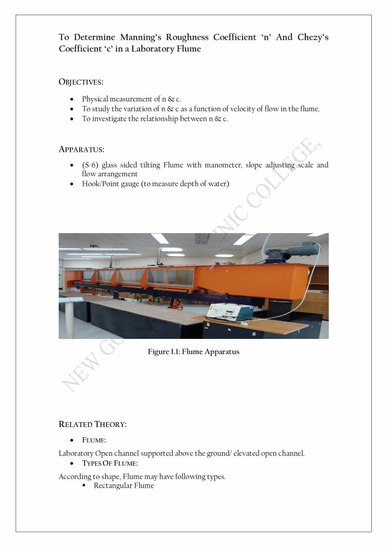
Figure 1.1: Flume Apparatus

RELATED THEORY:

FLUME:

Laboratory Open channel supported above the ground/ elevated open channel.

TYPES OF FLUME:

According to shape, Flume may have following types. Rectangular Flume

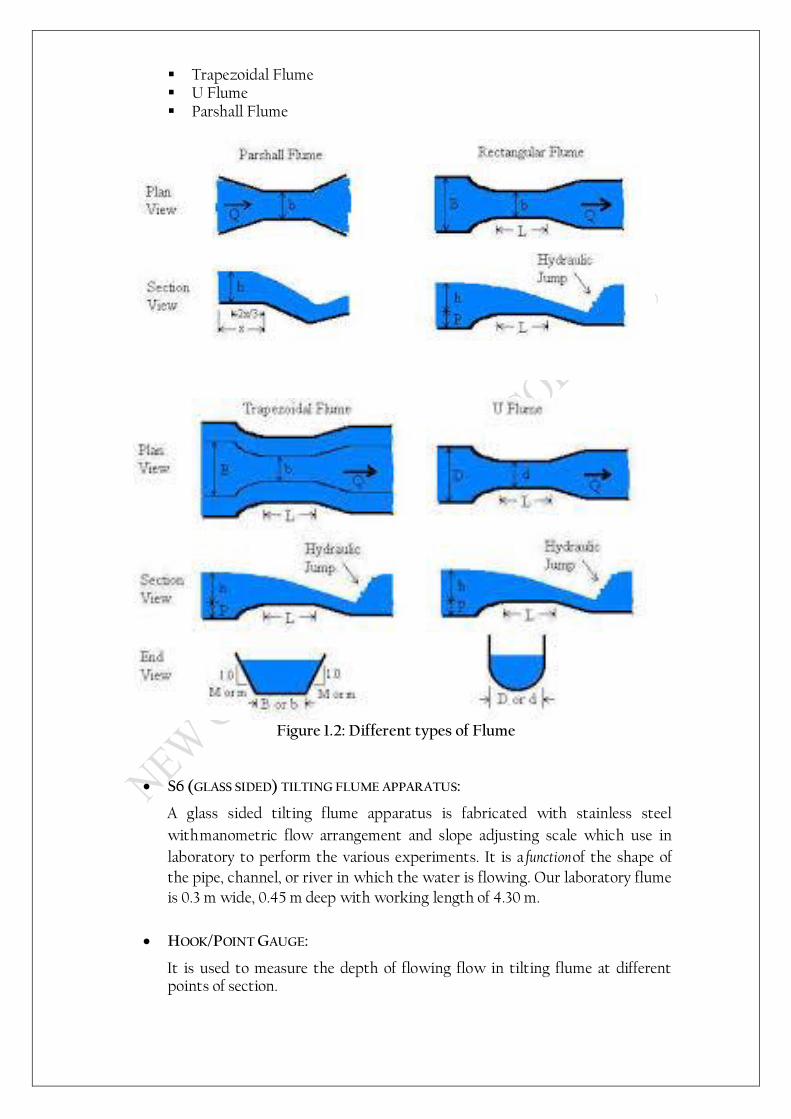
Trapezoidal Flume U Flume Parshall Flume

Figure 1.2: Different types of Flume

S6 (GLASS SIDED) TILTING FLUME APPARATUS:

A glass sided tilting flume apparatus is fabricated with stainless steel

with manometric flow arrangement and slope adjusting scale which use in

laboratory to perform the various experiments. It is a function of the shape of

the pipe, channel, or river in which the water is flowing. Our laboratory flume

is 0.3 m wide, 0.45 m deep with working length of 4.30 m.

HOOK/POINT GAUGE:

It is used to measure the depth of flowing flow in tilting flume at different points of section.

UNIFORM FLOW:

A uniform flow is one in which flow parameters and channel parameters remain same with respect to distance between two sections. This flow is only possible in prismatic flow.

NON UNIFORM FLOW:

A uniform flow is one in which flow parameters and channel parameters do not remain same with respect to distance between two sections. This flow is not possible in prismatic flow.

STEADY FLOW:

A steady flow is one in which the conditions (velocity, pressure and cross-section) may differ from point to point but do not change with time.

UNSTEADY FLOW:

A steady flow is one in which the conditions (velocity, pressure and cross-section) may differ from point to point but change with time.

STEADY UNIFORM FLOW:

Conditions do not change with position or with time in the stream. An example is the flow of water in a pipe of constant diameter at constant velocity.

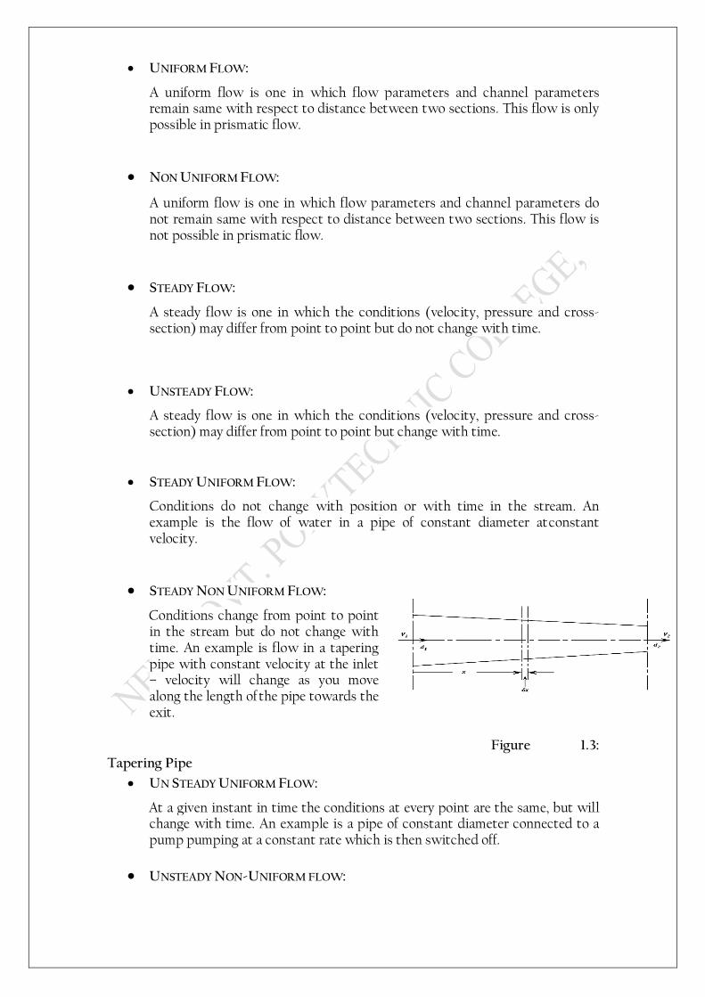
STEADY NON UNIFORM FLOW:

Conditions change from point to point in the stream but do not change with time. An example is flow in a tapering pipe with constant velocity at the inlet – velocity will change as you move along the length of the pipe towards the exit.

Figure 1.3:

Tapering Pipe

UN STEADY UNIFORM FLOW:

At a given instant in time the conditions at every point are the same, but will change with time. An example is a pipe of constant diameter connected to a pump pumping at a constant rate which is then switched off.

UNSTEADY NON-UNIFORM FLOW:

Every condition of the flow may change from point to point and with time at every point. For example waves in a channel.

MANNING’S ROUGHNESS FORMULA:

The Manning formula states that:

WHERE,

Q is the flow [L3/T] V is the cross-sectional average velocity [L/T] K is a conversion factor which is 1 in SI units. n is the Manning coefficient (also called as resistance to flow). R is the hydraulic radius [L] S is the slope of the water surface or the linear hydraulic head loss.

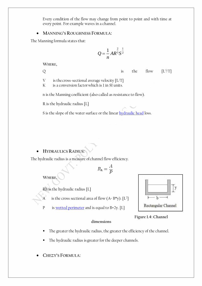
HYDRAULICS RADIUS:

The hydraulic radius is a measure of channel flow efficiency.

WHERE,

Rh is the hydraulic radius [L]

A is the cross sectional area of flow (A= B*y). [L2]

P is wetted perimeter and is equal to B+2y. [L]

Figure 1.4: Channel dimensions

The greater the hydraulic radius, the greater the efficiency of the channel.

The hydraulic radius is greater for the deeper channels.

CHEZY’S FORMULA:

2 1

3 21

Q AR Sn

http://en.wikipedia.org/wiki/Hydraulic_head

http://en.wikipedia.org/wiki/Wetted_perimeter

The Chezy’s formula states that:

FLOW RATE (DISCHARGE):

It is the amount of water in m3 passing in one second from a point.

Q= kA√ (2g∆h)

Where, K = roughness coefficient and here its value is 1.2 ∆h = h1 – h2 [L]

h1 = head of water in one limb of the pressure tube. (It’s a greater value). [L]

h2 = head of water in other limb of the pressure tube. (It’s a lesser value). [L]

RELATIONSHIP BETWEEN ‘n’ & ‘c’:

V = C RS , V = n

1R2/3S1/2

Comparing these equations………..

C RS = n

1R2/3S1/2

C = 2/12/1

2/13/2

.

..

1

SR

SR

n

C = 6/11R

n

PROCEDURE:

Set a particular slope of the flume.

Start the pump; allow the flow in the flume to be stabilized.

Determine the flow rate in the flume.

Take three readings of depth of flow in flume at different points and average it

for a particular flow rate in the flume.

Change the flow rate through the flume.

Again allow the flow in the flume to be stabilized.

Again take three readings of depth of flow in flume at different points and

average it.

Repeat the whole procedure (at least 5 readings) for different discharges in

the flume.

PRECAUTIONS:

Depth of flow should be measure at stabilized flow.

Slope in flume should be constant.

In the absence of point gauge, if depth of flow is being measured with scale,

then it should be placed at 900 angles with respect to the base of flume.

There should be no leakage of water from flume body while water is flowing.

OBSERVATIONS AND CALCULATIONS:

Flume width = B = ----------- m Value of k to find the Q = ----------

GRAPHICAL REPRESENTATION:

Sr. #

Bed slop

e (S)

Rise of water in tubes and

their difference

(m)

Average Depth of flow

Y= (Y1+Y2+Y3)/3 (m)

Wetted Perimet

er P=B+2Y

(m)

Area of

flow A=

(B*Y) (m2)

Hydraulic mean Radi

us R= A/P (m)

Flow rate Q=

kA√(2g∆h)

(m3/sec)

Manning’s

Constant n=

AR2/3S1/2/Q

Chezy’s Consta

nt c=

R1/6/n

h1

h2

∆h

Y1 Y2 Y3 Y

1

2

3

4

5

a) Graph between Q and n

(b) Graph between Q and C

(c) Graph between n and C

RESULTS:

COMMENTS:

EXPERIMENT NO. 6

HYDRAULIC JUMP ANALYSIS

OBJECTIVE:

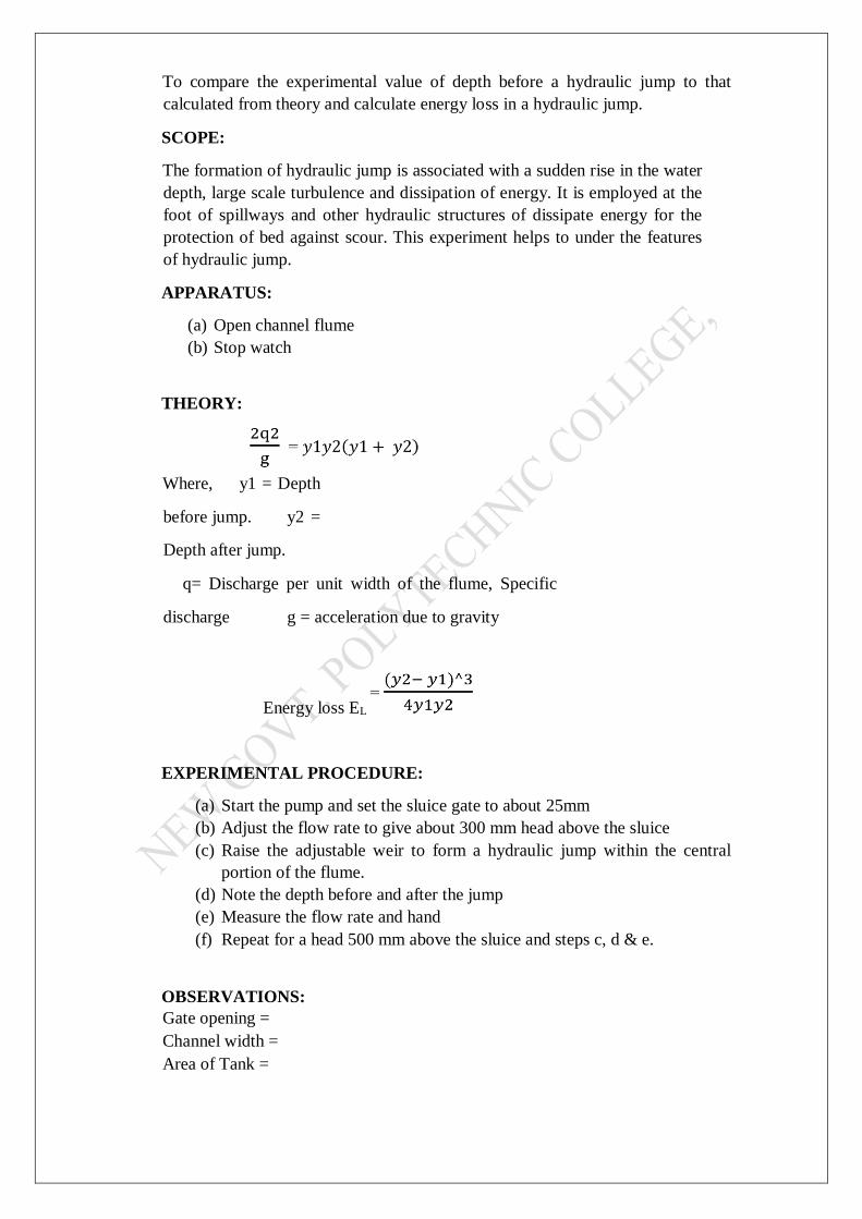
To compare the experimental value of depth before a hydraulic jump to that

calculated from theory and calculate energy loss in a hydraulic jump.

SCOPE:

The formation of hydraulic jump is associated with a sudden rise in the water

depth, large scale turbulence and dissipation of energy. It is employed at the

foot of spillways and other hydraulic structures of dissipate energy for the

protection of bed against scour. This experiment helps to under the features

of hydraulic jump.

APPARATUS:

(a) Open channel flume

(b) Stop watch

THEORY:

Where, y1 = Depth

before jump. y2 =

Depth after jump.

q= Discharge per unit width of the flume, Specific

discharge g = acceleration due to gravity

Energy loss EL

EXPERIMENTAL PROCEDURE:

(a) Start the pump and set the sluice gate to about 25mm

(b) Adjust the flow rate to give about 300 mm head above the sluice

(c) Raise the adjustable weir to form a hydraulic jump within the central

portion of the flume.

(d) Note the depth before and after the jump

(e) Measure the flow rate and hand

(f) Repeat for a head 500 mm above the sluice and steps c, d & e.

OBSERVATIONS:

Gate opening =

Channel width =

Area of Tank =

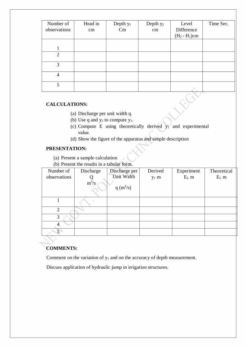
Number of

observations

Head in

cm

Depth y1

Cm

Depth y2

cm

Level

Difference

(H2 - H1)cm

Time Sec.

1

2

3

4

5

CALCULATIONS:

(a) Discharge per unit width q.

(b) Use q and y2 to compute y1.

(c) Compute E using theoretically derived y1 and experimental

value.

(d) Show the figure of the apparatus and simple description

PRESENTATION:

(a) Present a sample calculation

(b) Present the results in a tabular form.

Number of

observations

Discharge

Q

m3/s

Discharge per

Unit Width

q (m3/s)

Derived

y1 m

Experiment

EL m

Theoretical

EL m

1

2

3

4

5

COMMENTS:

Comment on the variation of y1 and on the accuracy of depth measurement.

Discuss application of hydraulic jump in irrigation structures.

EX. NO-7

FLOW THROUGH NOTCHES

OBJECTIVES:

To determine the coefficients of discharge of the rectangular, triangular and

trapezoidal notches.

APPARATUS REQUIRED:

Hydraulic bench

Notches – Rectangular, triangular, trapezoidal shape.

Hook and point gauge

Calibrated collecting tank

Stop watch

THEORY:

A notch is a sharp-edged device used for the measurement of discharge in free surface

flows. A notch can be of different shapes – rectangular, triangular, trapezoidal etc. A

triangular notch is particularly suited for measurement of small discharges. The

discharge over a notch mainly depends on the head H, relative to the crest of the

notch, measured upstream at a distance about 3 to 4 times H from the crest. General

formula can be obtained for a symmetrical trapezoidal notch which is a combined

shape of rectangular and triangular notches. By applying the Bernoulli Equation

(conservation of energy equation) to a simplified flow model of a symmetric

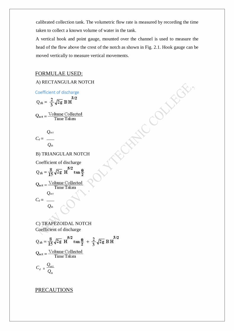
trapezoidal notch, theoretical discharge Qth is obtained as:

. . . . . . . . . .. . . . . . (1)

Where ‘H’ is the water head measured above the crest, ‘θ’ is the angle between the

side edges and ‘B’ is the bottom width of the notch.

When θ=0, this equation is reduced and applicable for rectangular notch or when B=0

(no bottom width) it is applicable for triangular notch. Hence the same equation (1)

can be also used for both rectangular and triangular notches by substituting

corresponding values (ie θ=0 or B=0).

If Qact actual discharge is known then coefficient of discharge Cd of the notch can be

expressed as Cd = Qact/Qth.

DESCRIPTION

In open channel hydraulics, weirs are commonly used to either regulate or to measure

the volumetric flow rate. They are of particular use in large scale situations such as

irrigation schemes, canals and rivers. For small scale applications, weirs are often

referred to as notches and invariably are sharp edged and manufactured from thin

plate material. Water enters the stilling baffles which calms the flow. Then, the flow

passes into the channel and flows over a sharp-edged notch set at the other end of the

channel. Water comes of the channel in the form of a nappe is then directed into the

calibrated collection tank. The volumetric flow rate is measured by recording the time

taken to collect a known volume of water in the tank.

A vertical hook and point gauge, mounted over the channel is used to measure the

head of the flow above the crest of the notch as shown in Fig. 2.1. Hook gauge can be

moved vertically to measure vertical movements.

FORMULAE USED:

A) RECTANGULAR NOTCH

Coefficient of discharge

Qact

Cd =

Qth

B) TRIANGULAR NOTCH


Qact

Cd =

Qth

C) TRAPEZOIDAL NOTCH

PRECAUTIONS


th

act d

Q

Q C =

• Ensure and read initial water level reading just above the crest.

PROCEDURE (INSTRUCTIONAL MODE)

Preparation for experiment:

1. Insert the given notch into the hydraulic bench and fit tightly by using bolts in

order to prevent leakage.

2. Open the water supply and allow water till over flows over the notch. Stop

water supply, let excess water drain through notch and note the initial reading

of the water level ‘h0’using the hook and point gauge. Let water drain from

collecting tank and shut the valve of collecting tank after emptying the

collecting tank.

Experiment steps:

3. After initial preparation, open regulating valve to increase the flow and

maintain water level over notch. Wait until flow is steady.

4. Move hook and point gauge vertically and measure the current water level ‘h1’

to find the water head ‘H’ above the crest of the notch.

5. Note the piezometric reading ‘z0’ in the collecting tank while switch on the

stopwatch.

6. Record the time taken ‘T’ and the piezometric reading ‘z1’ in the collecting

tank after allowing sufficient water quantity of water in the collecting tank.

7. Repeat step 3 to step 6 by using different flow rate of water, which can be

done by adjusting the water supply. Measure and record the H, the time and

piezometric reading in the collecting tank until 5 sets of data have been taken.

If collecting tank is full, just empty it before the step no 3.

8. To determine the coefficient of discharge for the other notch, repeat from step

1.

After entering the readings in the Tabulation 2.1 and Tabulation 2.2, compute the

necessary values.


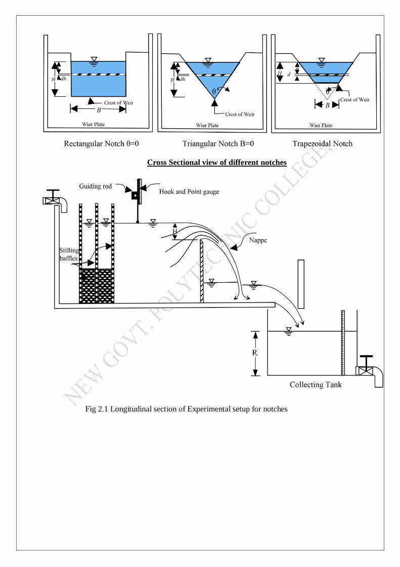
Cross Sectional view of different notches

Fig 2.1 Longitudinal section of Experimental setup for notches

2. FLOW THROUGH NOTCHES

35

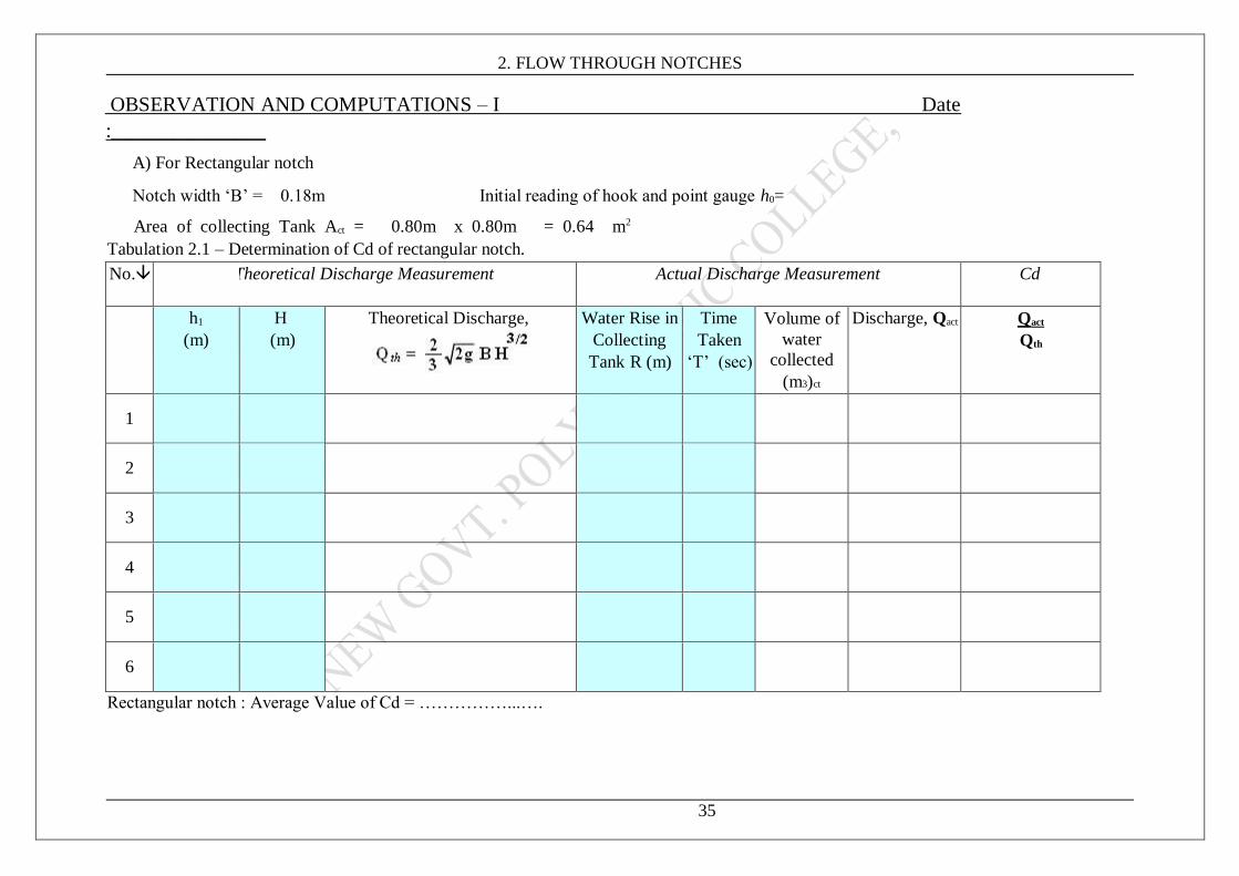
OBSERVATION AND COMPUTATIONS – I Date

:_______________

A) For Rectangular notch

Notch width ‘B’ = 0.18m Initial reading of hook and point gauge h0=

Area of collecting Tank Act = 0.80m x 0.80m = 0.64 m2

Tabulation 2.1 – Determination of Cd of rectangular notch.

No. Theoretical Discharge Measurement Actual Discharge Measurement Cd

h1

(m)

H

(m)

Theoretical Discharge,

Water Rise in

Collecting

Tank R (m)

Time

Taken

‘T’ (sec)

Volume of

water

collected

(m3)ct

Discharge, Qact Qact

Qth

1

2

3

4

5

6

Rectangular notch : Average Value of Cd = ……………...….


36

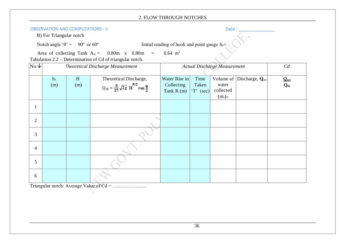
OBSERVATION AND COMPUTATIONS - II Date : _______________

B) For Triangular notch

Notch angle ‘θ’ = 90º or 60º Initial reading of hook and point gauge h0=

Area of collecting Tank Act = 0.80m x 0.80m = 0.64 m2

Tabulation 2.2 – Determination of Cd of triangular notch.


h1

(m)

H

(m)


Water Rise in

Collecting

Tank R (m)

Time

Taken

‘T’ (sec)

Volume of

water

collected

(m3)ct


Qth

1

2

3

4

5

6

Triangular notch: Average Value of Cd = ……………...….


37

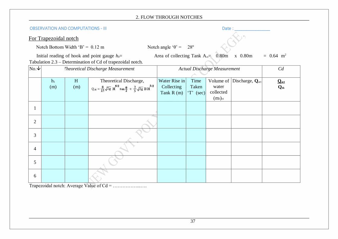
OBSERVATION AND COMPUTATIONS - III Date : _______________

For Trapezoidal notch

Notch Bottom Width ‘B’ = 0.12 m Notch angle ‘θ’ = 28º

Initial reading of hook and point gauge h0= Area of collecting Tank Act= 0.80m x 0.80m = 0.64 m2

Tabulation 2.3 – Determination of Cd of trapezoidal notch.


h1

(m)

H

(m)


Water Rise in

Collecting

Tank R (m)

Time

Taken

‘T’ (sec)

Volume of

water

collected

(m3)ct


Qth

1

2

3

4

5

6

Trapezoidal notch: Average Value of Cd = ……………...….



GRAPH:

1- Cd versus Qact curves are drawn taking Qact on x -axis and Cd on y – axis in the

same graph for all the notches.

2- Qact versus H curves are drawn taking H on x -axis and Qact

on y – axis in the

same graph for all the notches.


39

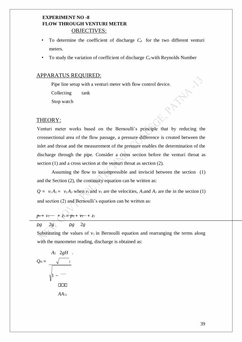
EXPERIMENT NO -8

FLOW THROUGH VENTURI METER

OBJECTIVES:

• To determine the coefficient of discharge Cd for the two different venturi

meters.

• To study the variation of coefficient of discharge Cd with Reynolds Number

APPARATUS REQUIRED:

Pipe line setup with a venturi meter with flow control device.

Collecting tank

Stop watch

THEORY:

Venturi meter works based on the Bernoulli’s principle that by reducing the

crosssectional area of the flow passage, a pressure difference is created between the

inlet and throat and the measurement of the pressure enables the determination of the

discharge through the pipe. Consider a cross section before the venturi throat as

section (1) and a cross section at the venturi throat as section (2).

Assuming the flow to incompressible and inviscid between the section (1)

and the Section (2), the continuity equation can be written as:

Q = v1 A1 = v2 A2 when v1 and v2 are the velocities, A1and A2 are the in the section (1)

and section (2) and Bernoulli’s equation can be written as:

p1 + v1 + z1 = p2 + v2 + z2

ρg 2g ρg 2g

Substituting the values of v1 in Bernoulli equation and rearranging the terms along

with the manometer reading, discharge is obtained as:

A2 2gH .

Qth = 2

1 −

AA12

40

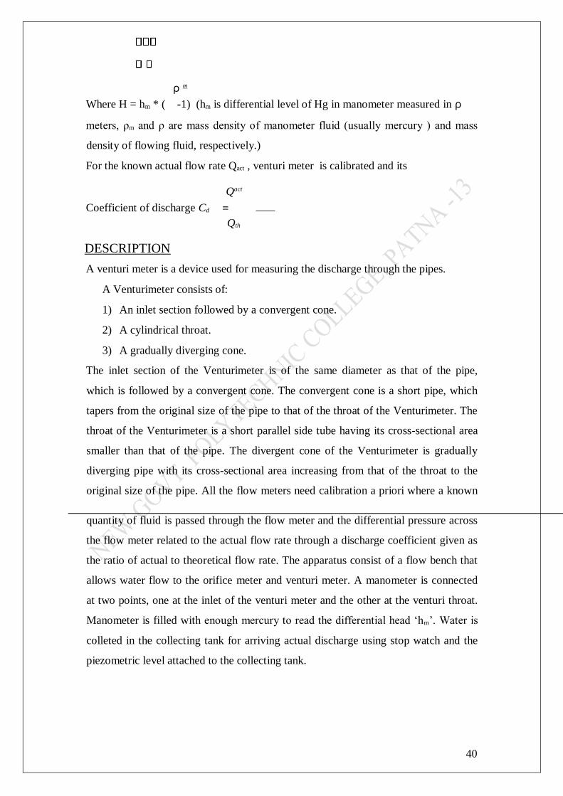
ρ m

Where H = hm * ( -1) (hm is differential level of Hg in manometer measured in ρ

meters, ρm and ρ are mass density of manometer fluid (usually mercury ) and mass

density of flowing fluid, respectively.)

For the known actual flow rate Qact , venturi meter is calibrated and its

Qact

Coefficient of discharge Cd =

Qth

DESCRIPTION

A venturi meter is a device used for measuring the discharge through the pipes.

A Venturimeter consists of:

1) An inlet section followed by a convergent cone.

2) A cylindrical throat.

3) A gradually diverging cone.

The inlet section of the Venturimeter is of the same diameter as that of the pipe,

which is followed by a convergent cone. The convergent cone is a short pipe, which

tapers from the original size of the pipe to that of the throat of the Venturimeter. The

throat of the Venturimeter is a short parallel side tube having its cross-sectional area

smaller than that of the pipe. The divergent cone of the Venturimeter is gradually

diverging pipe with its cross-sectional area increasing from that of the throat to the

original size of the pipe. All the flow meters need calibration a priori where a known

quantity of fluid is passed through the flow meter and the differential pressure across

the flow meter related to the actual flow rate through a discharge coefficient given as

the ratio of actual to theoretical flow rate. The apparatus consist of a flow bench that

allows water flow to the orifice meter and venturi meter. A manometer is connected

at two points, one at the inlet of the venturi meter and the other at the venturi throat.

Manometer is filled with enough mercury to read the differential head ‘hm’. Water is

colleted in the collecting tank for arriving actual discharge using stop watch and the

piezometric level attached to the collecting tank.

41

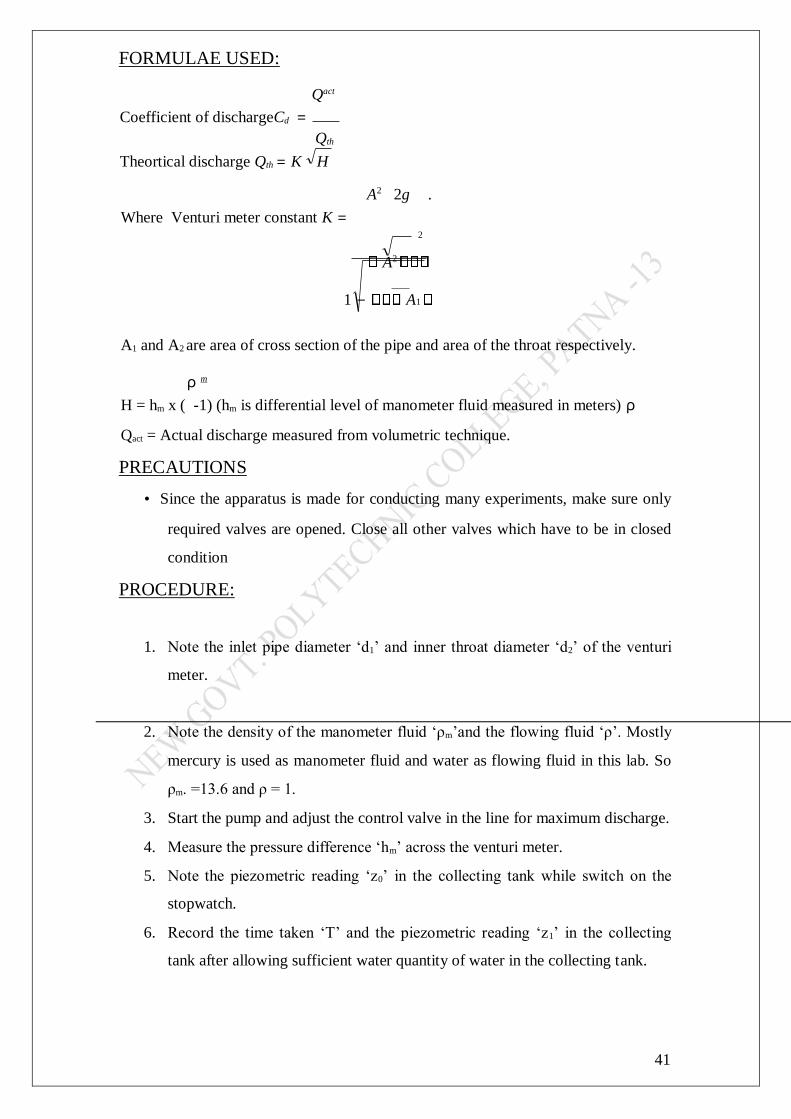
FORMULAE USED:

Qact

Coefficient of dischargeCd =

Qth

Theortical discharge Qth = K H

A2 2g .

Where Venturi meter constant K = 2

A2

1 − A1

A1 and A2 are area of cross section of the pipe and area of the throat respectively.

ρ m

H = hm x ( -1) (hm is differential level of manometer fluid measured in meters) ρ

Qact = Actual discharge measured from volumetric technique.

PRECAUTIONS

• Since the apparatus is made for conducting many experiments, make sure only

required valves are opened. Close all other valves which have to be in closed

condition

PROCEDURE:

1. Note the inlet pipe diameter ‘d1’ and inner throat diameter ‘d2’ of the venturi

meter.

2. Note the density of the manometer fluid ‘ρm’and the flowing fluid ‘ρ’. Mostly

mercury is used as manometer fluid and water as flowing fluid in this lab. So

ρm. =13.6 and ρ = 1.

3. Start the pump and adjust the control valve in the line for maximum discharge.

4. Measure the pressure difference ‘hm’ across the venturi meter.

5. Note the piezometric reading ‘z0’ in the collecting tank while switch on the

stopwatch.

6. Record the time taken ‘T’ and the piezometric reading ‘z1’ in the collecting

tank after allowing sufficient water quantity of water in the collecting tank.

42

7. Decrease the flow rate through the system by regulating the control valve and

wait till flow is steady.

8. Repeat the steps 4 to 6 for 5 different flow rates.

After entering the readings in the Tabulation 7.1 and 7.2, compute the necessary

values.


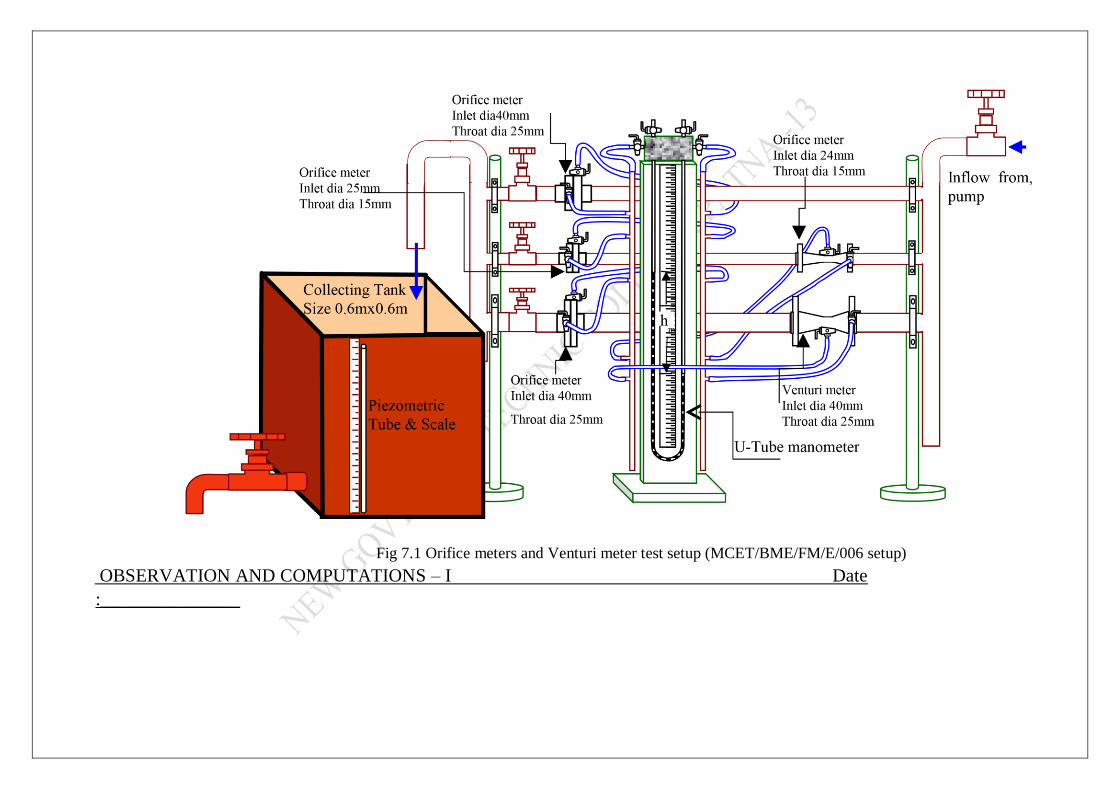
Fig 7.1 Orifice meters and Venturi meter test setup (MCET/BME/FM/E/006 setup)


:_______________

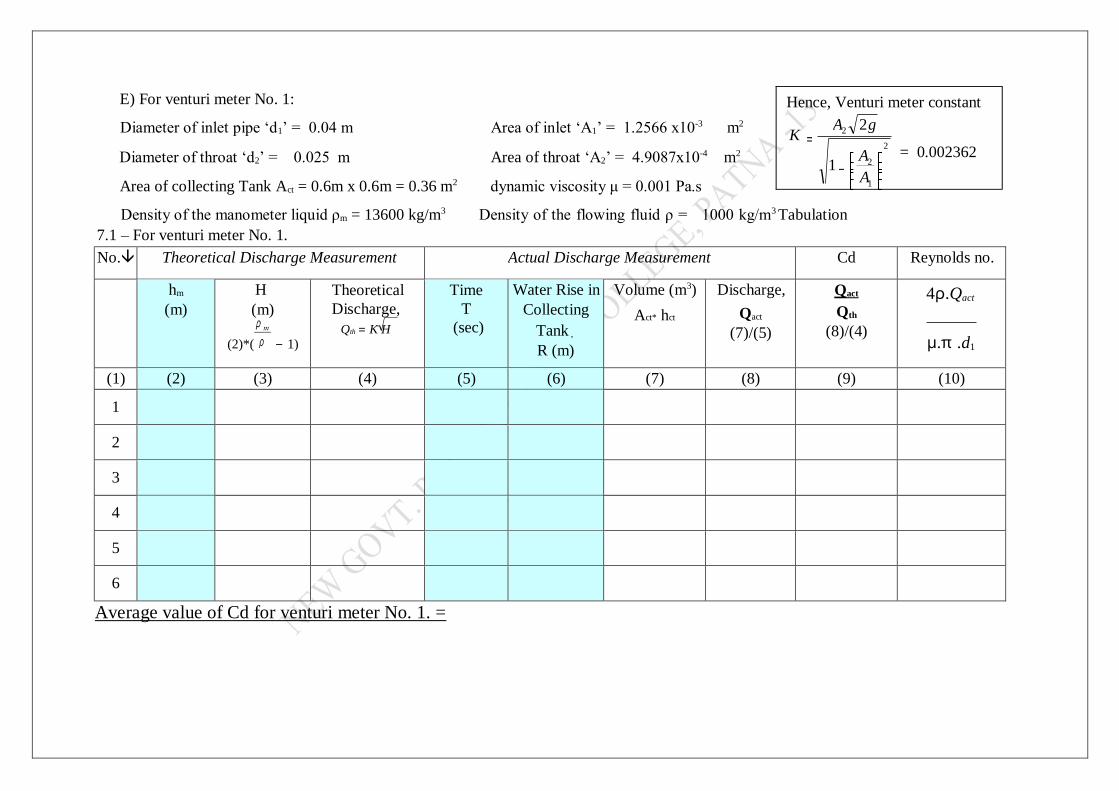
E) For venturi meter No. 1:

Diameter of inlet pipe ‘d1’ = 0.04 m Area of inlet ‘A1’ = 1.2566 x10-3 m2

Diameter of throat ‘d2’ = 0.025 m Area of throat ‘A2’ = 4.9087x10-4 m2

Area of collecting Tank Act = 0.6m x 0.6m = 0.36 m2 dynamic viscosity μ = 0.001 Pa.s

Density of the manometer liquid ρm = 13600 kg/m3 Density of the flowing fluid ρ = 1000 kg/m3 Tabulation

7.1 – For venturi meter No. 1.

No. Theoretical Discharge Measurement Actual Discharge Measurement Cd Reynolds no.

hm

(m)

H

(m)

(2)*( − 1)

Theoretical

Discharge,

Qth = K H

Time

T

(sec)

Water Rise in

Collecting

Tank ,

R (m)

Volume (m3)

Act* hct

Discharge,

Qact

(7)/(5)

Qact

Qth

(8)/(4)

4ρ.Qact

µ.π .d1

(1) (2) (3) (4) (5) (6) (7) (8) (9) (10)

1

2

3

4

5

6

Average value of Cd for venturi meter No. 1. =

Hence, Venturi meter constant

2

1

2

2

1

2

−

=

A

A

g A K

= 0.002362

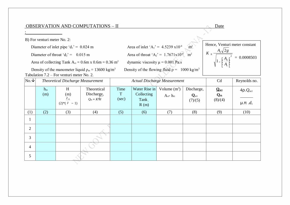
OBSERVATION AND COMPUTATIONS – II Date

:_______________

B) For venturi meter No. 2:

Diameter of inlet pipe ‘d1’ = 0.024 m Area of inlet ‘A1’ = 4.5239 x10-4 m2

Diameter of throat ‘d2’ = 0.015 m Area of throat ‘A2’ = 1.7671x10-4 m2

Area of collecting Tank Act = 0.6m x 0.6m = 0.36 m2 dynamic viscosity μ = 0.001 Pa.s

Density of the manometer liquid ρm = 13600 kg/m3 Density of the flowing fluid ρ = 1000 kg/m3

Tabulation 7.2 – For venturi meter No. 2.

No. Theoretical Discharge Measurement Actual Discharge Measurement Cd Reynolds no.

hm

(m)

H

(m)

(2)*( − 1)

Theoretical

Discharge,

Qth = K H

Time

T

(sec)

Water Rise in

Collecting

Tank ,

R (m)

Volume (m3)

Act* hct

Discharge,

Qact

(7)/(5)

Qact

Qth

(8)/(4)

4ρ.Qact

µ.π .d1

(1) (2) (3) (4) (5) (6) (7) (8) (9) (10)

1

2

3

4

5

Hence, Venturi meter constant

2

1

2

2

1

2

−

=

A

A

g A K

= 0.0008503

6

Average value of Cd for venturi meter No. 2.=

7. FLOW THROUGH VENTURI METER

GRAPH:

1- Cd vs. Qact are drawn in the same graph for both the venturi meters taking Qact on

x -axis and Cd on y – axis.

2- Qact vs. H are drawn in the same graph for both the venturi meters taking H on x -

axis and Qact on y – axis.


9.PERFORMANCE TEST ON CENTRIFUGAL PUMP OBJECTIVES:

To study the operation of centrifugal pump and to obtain the performance

characteristic curves.

APPARATUS REQUIRED:

Centrifugal pump with pressure gauge and vacuum gauge setup.

Stop Watch

Collecting tank

Scale

Tachometer

Energy meter

THEORY:

A centrifugal pump is a rotodynamic pump that uses a rotating impeller to increase

the pressure of a fluid. The pump works by the conversion of the rotational kinetic

energy, typically from an electric motor or turbine, to an increased static fluid

pressure. This action is described by Bernoulli's principle. The rotation of the pump

impeller imparts kinetic energy to the fluid as it is drawn in from the impeller eye and

is forced outward through the impeller vanes to the periphery. As the fluid exits the

impeller, the fluid kinetic energy is then converted to pressure due to the change in

area the fluid experiences in the volute section. The energy conversion, results in an

increased pressure on the delivery side of the pump, causes the flow.

DESCRIPTION

The test pump is a single stage centrifugal pump. It is coupled with an electric motor

by means cone pulley belt drive system. An energy meter is permanently connected

to measure the energy consumed by the electric motor for driving the pump. A stop

watch is provided to measure the input power to the pump. A pressure gauge and a

vacuum gauge are fitted it the delivery and suction pipes, respectively, to measure the

pressure.

FORMULAE USED:

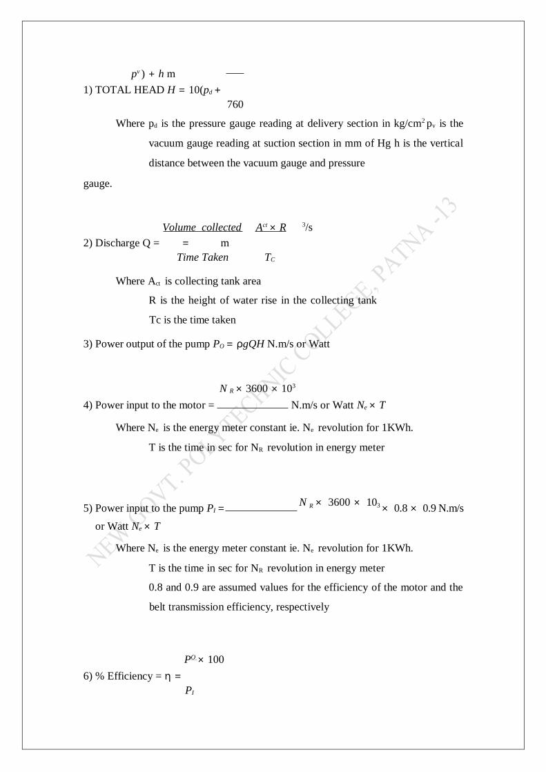
pv ) + h m

1) TOTAL HEAD H = 10(pd +

760

Where pd is the pressure gauge reading at delivery section in kg/cm2 pv is the

vacuum gauge reading at suction section in mm of Hg h is the vertical

distance between the vacuum gauge and pressure

gauge.

Volume collected Act × R 3/s

2) Discharge Q = = m

Time Taken TC

Where Act is collecting tank area

R is the height of water rise in the collecting tank

Tc is the time taken

3) Power output of the pump PO = ρgQH N.m/s or Watt

N R × 3600 × 103

4) Power input to the motor = N.m/s or Watt Ne × T

Where Ne is the energy meter constant ie. Ne revolution for 1KWh.

T is the time in sec for NR revolution in energy meter

5) Power input to the pump PI = N R × 3600 × 103 × 0.8 × 0.9 N.m/s

or Watt Ne × T



0.8 and 0.9 are assumed values for the efficiency of the motor and the

belt transmission efficiency, respectively

PO × 100

6) % Efficiency = η =

PI

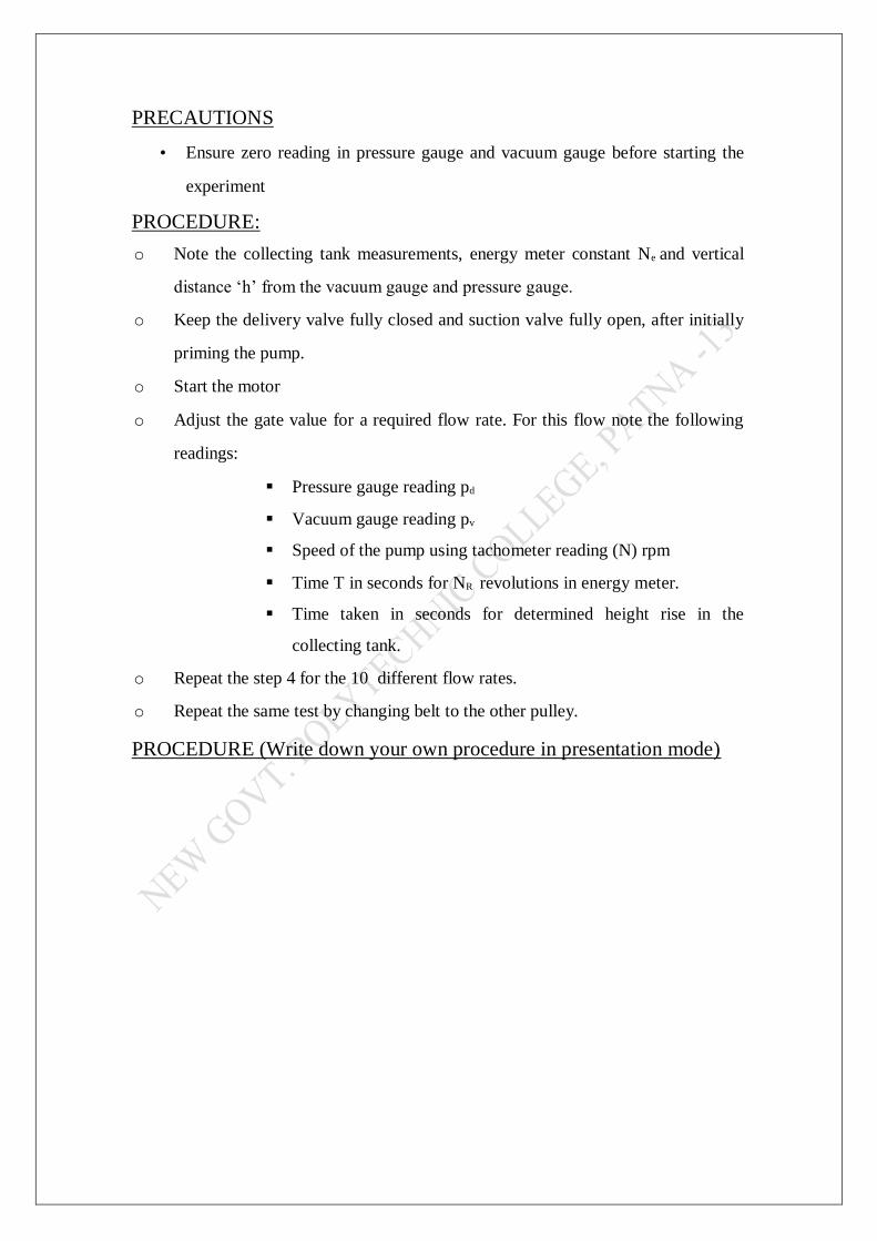
PRECAUTIONS

• Ensure zero reading in pressure gauge and vacuum gauge before starting the

experiment

PROCEDURE:

o Note the collecting tank measurements, energy meter constant Ne and vertical

distance ‘h’ from the vacuum gauge and pressure gauge.

o Keep the delivery valve fully closed and suction valve fully open, after initially

priming the pump.

o Start the motor

o Adjust the gate value for a required flow rate. For this flow note the following

readings:

Pressure gauge reading pd

Vacuum gauge reading pv

Speed of the pump using tachometer reading (N) rpm

Time T in seconds for NR revolutions in energy meter.

Time taken in seconds for determined height rise in the

collecting tank.

o Repeat the step 4 for the 10 different flow rates.

o Repeat the same test by changing belt to the other pulley.


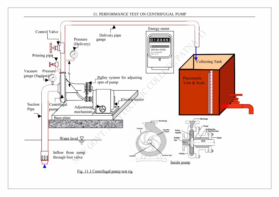
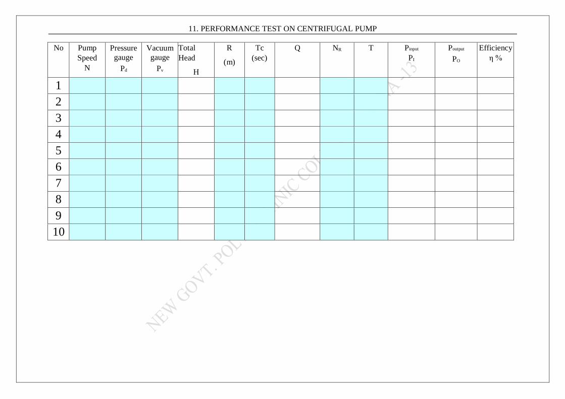
11. PERFORMANCE TEST ON CENTRIFUGAL PUMP


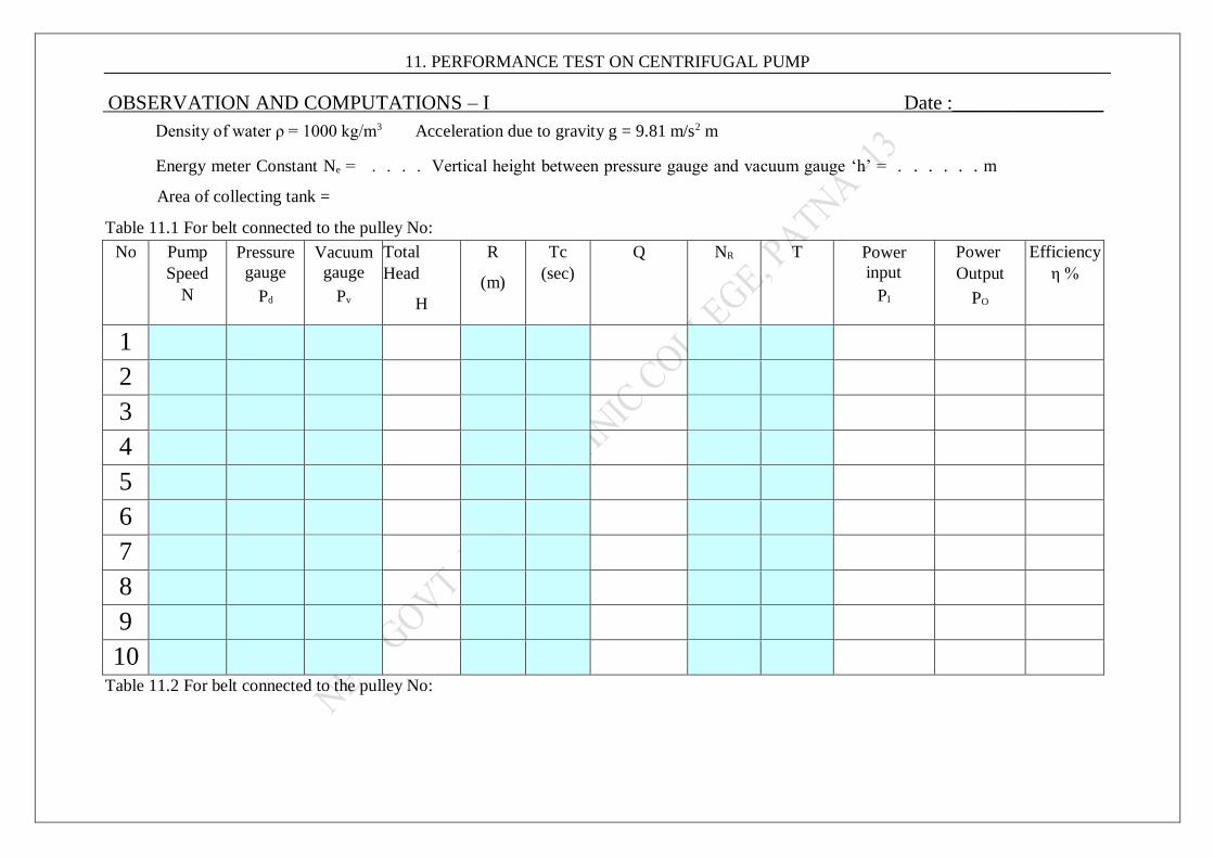
OBSERVATION AND COMPUTATIONS – I Date :_______________

Density of water ρ = 1000 kg/m3 Acceleration due to gravity g = 9.81 m/s2 m

Energy meter Constant Ne = . . . . Vertical height between pressure gauge and vacuum gauge ‘h’ = . . . . . . m

Area of collecting tank =

Table 11.1 For belt connected to the pulley No:

No Pump

Speed

N

Pressure

gauge

Pd

Vacuum

gauge

Pv

Total

Head

H

R

(m)

Tc

(sec)

Q NR T Power

input

PI

Power

Output

PO

Efficiency

η %

1

2

3

4

5

6

7

8

9

10



No Pump

Speed

N

Pressure

gauge

Pd

Vacuum

gauge

Pv

Total

Head

H

R

(m)

Tc

(sec)

Q NR T Pinput

PI

Poutput

PO

Efficiency

η %

1

2

3

4

5

6

7

8

9

10


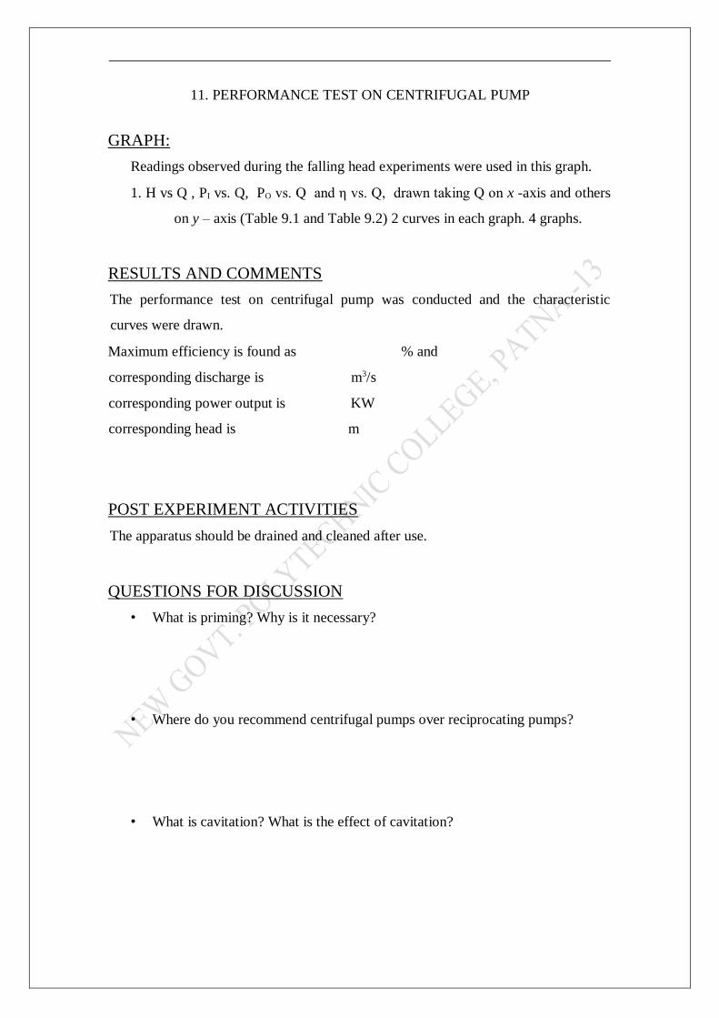
GRAPH:

Readings observed during the falling head experiments were used in this graph.

1. H vs Q , PI vs. Q, PO vs. Q and η vs. Q, drawn taking Q on x -axis and others

on y – axis (Table 9.1 and Table 9.2) 2 curves in each graph. 4 graphs.


The performance test on centrifugal pump was conducted and the characteristic

curves were drawn.

Maximum efficiency is found as % and

corresponding discharge is m3/s

corresponding power output is KW

corresponding head is m

POST EXPERIMENT ACTIVITIES

The apparatus should be drained and cleaned after use.

QUESTIONS FOR DISCUSSION

• What is priming? Why is it necessary?

• Where do you recommend centrifugal pumps over reciprocating pumps?

• What is cavitation? What is the effect of cavitation?

EXPERIENT NO -10

PERFORMANCE TEST ON RECIPROCATING PUMP

OBJECTIVES:

To conduct the performance test and there by study the characteristics of the

reciprocating pump.

APPARATUS REQUIRED:

Reciprocating pump with pressure gauge and vacuum gauge setup.

Stop Watch

Collecting tank

Scale

Tachometer

Energy meter

THEORY:

A reciprocating pump is a positive displacement type pump, because of the liquid is

sucked and displaced due to the thrust exerted on it by a moving piston inside the

cylinder. The cylinder has two one-way valves, one for allowing water into the

cylinder from the suction pipe and the other for discharging water from the cylinder

to the delivery pipe. The pump operates in two strokes. During suction stroke, the

suction valve opens and delivery valve closes while the piston move away from the

valve. This movement creates low pressure/partial vacuum inside the cylinder hence

water enters through suction valve. During delivery stroke, the piston moves towards

the valves. Due to this, the suction valve closes and the delivery valve opens, hence

liquid is delivered through delivery valve to the delivery pipe.

DESCRIPTION

The reciprocating pipe consists of a pump cylinder, piston, piston rod, crank,

connecting rod, suction pipe, delivery pipe, suction valve and delivery valve. It is

coupled with an electric motor by means cone pulley belt drive system. An energy

meter is permanently connected to measure the energy consumed by the electric

motor for driving the pump. A stop watch is provided to measure the input power to

the pump. A pressure gauge and a vacuum gauge are fitted it the delivery and suction

pipes, respectively, to measure the pressure.

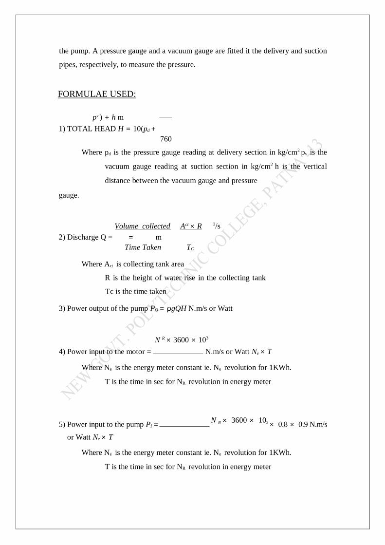
FORMULAE USED:

pv ) + h m

1) TOTAL HEAD H = 10(pd +

760

Where pd is the pressure gauge reading at delivery section in kg/cm2 pv is the

vacuum gauge reading at suction section in kg/cm2 h is the vertical

distance between the vacuum gauge and pressure

gauge.

Volume collected Act × R 3/s

2) Discharge Q = = m

Time Taken TC

Where Act is collecting tank area

R is the height of water rise in the collecting tank

Tc is the time taken

3) Power output of the pump PO = ρgQH N.m/s or Watt

N R × 3600 × 103

4) Power input to the motor = N.m/s or Watt Ne × T



5) Power input to the pump PI = N R × 3600 × 103 × 0.8 × 0.9 N.m/s

or Watt Ne × T



0.8 and 0.9 are assumed values for the efficiency of the motor and the

belt transmission efficiency, respectively

PO × 100

6) % Efficiency = η =

PI

PRECAUTIONS

• Ensure zero reading in pressure gauge and vacuum gauge before starting the

experiment

PROCEDURE:

o Note the collecting tank measurements, energy meter constant Ne and vertical

distance ‘h’ from the vacuum gauge and pressure gauge.

o Keep the delivery valve fully closed and suction valve fully open, after initially

priming the pump.

o Start the motor

o Adjust the gate value for a required flow rate. For this flow note the following

readings:

Pressure gauge reading pd

Vacuum gauge reading pv

Speed of the pump using tachometer reading (N) rpm

Time T in seconds for NR revolutions in energy meter.

Time taken in seconds for determined height rise in the

collecting tank.

o Repeat the step 4 for the 10 different flow rates.

o Repeat the same test by changing belt to the other pulley.


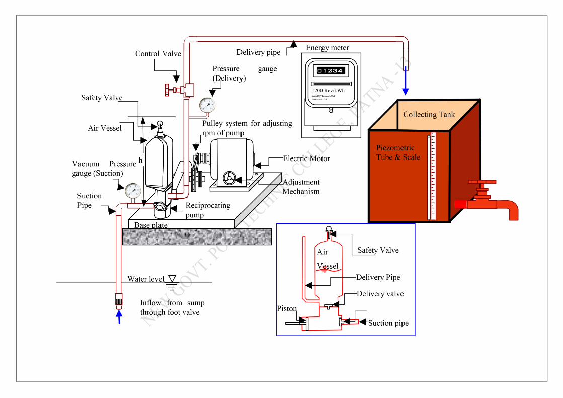
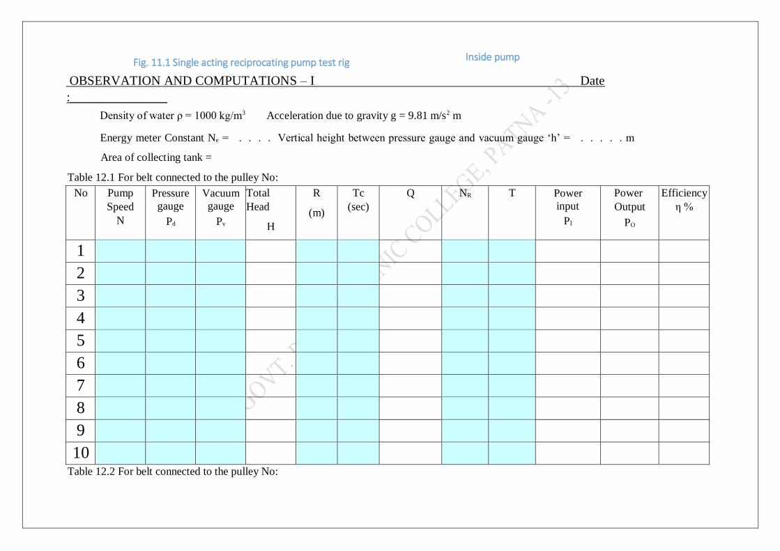
Fig. 11.1 Single acting reciprocating pump test rig Inside pump


:_______________

Density of water ρ = 1000 kg/m3 Acceleration due to gravity g = 9.81 m/s2 m

Energy meter Constant Ne = . . . . Vertical height between pressure gauge and vacuum gauge ‘h’ = . . . . . m

Area of collecting tank =


No Pump

Speed

N

Pressure

gauge

Pd

Vacuum

gauge

Pv

Total

Head

H

R

(m)

Tc

(sec)

Q NR T Power

input

PI

Power

Output

PO

Efficiency

η %

1

2

3

4

5

6

7

8

9

10


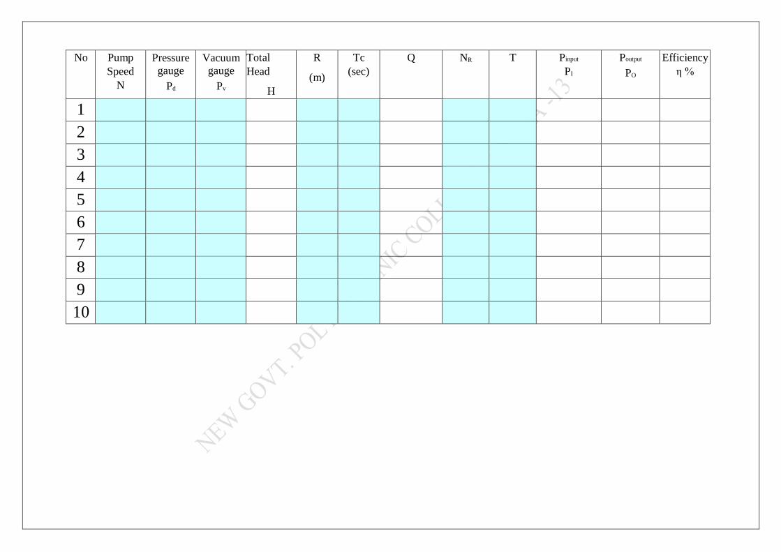
No Pump

Speed

N

Pressure

gauge

Pd

Vacuum

gauge

Pv

Total

Head

H

R

(m)

Tc

(sec)

Q NR T Pinput

PI

Poutput

PO

Efficiency

η %

1

2

3

4

5

6

7

8

9

10

PERFORMANCE TEST ON RECIPROCATING PUMP

GRAPH:

Readings observed during the falling head experiments were used in this graph.

1. H vs Q , PI vs. Q, PO vs. Q and η vs. Q, drawn taking Q on x -axis and others on y – axis

(Table 9.1 and Table 9.2) 2 curves in each graph. 4 graphs.


The performance test on reciprocating pump was conducted and the characteristic curves were

drawn.

Maximum efficiency is found as % and corresponding discharge is

m3/s corresponding power output is KW corresponding head is

new government polytechnic college, patna -13 lab …

Documents