new insight into the dynamics of water and macromolecules ... · pdf filenew insight into the...

IJRRAS 23 (3) ● June 2015 www.arpapress.com/Volumes/Vol23Issue3/IJRRAS_23_3_05.pdf

207

NEW INSIGHT INTO THE DYNAMICS OF WATER AND

MACROMOLECULES IN MEAT DURING DRIP AS PROBED BY

PROTON CPMG NMR

Eddy W. Hansen1,* & Han Zhu2, 3 1Department of Chemistry, University of Oslo, P.O. BOX 1033, Blindern, N-0315 Oslo, Norway

2Department of Chemistry, Biotechnology and Food Science, Norwegian University of Life Sciences, P.O. Box

5003, 1432- Ås, Norway 3Nortura SA, Lørenveien 37, Økern, 0585 Oslo, Norway

ABSTRACT

BACKGROUND: Three distinct proton spin-spin relaxation rate components in meat are known to be associated with

three corresponding spatial domains possessing different molecular ratios of water and/or macromolecules (extra- and

inter/intramyofibrillar). In this work we acquire the proton signal intensity and corresponding relaxation rate of the

three components during a drip experiment with the objective to probe the irreversible migration of water and

macromolecules between domains with drip time.

RESULTS: Each CPMG relaxation curve is decomposed into three relevant and distinct relaxation components

(intensity and relaxation rate). A first-order kinetic model is adopted which enables the irreversible and slow

“migration” of water and macromolecules between domains to be monitored. A detailing of the kinetic model applied

is thoroughly discussed.

CONCLUSIONS: The amount of water and macromolecules within the respective domains in meat is monitored and

quantified by in situ CPMG measurements during drip. The observed and irreversible change in proton

intensity/relaxation rate during drip is rationalized by a slow migration of water molecules and macromolecules

between the domains.

GENERAL SIGNIFICANCE: To shed new light on the water holding capacity in biological material by probing the

slow migration properties of water/macromolecules between different domains during drip loss.

Keywords: Water holding capacity; relaxation rates; kinetic model; relaxation sink; drip loss; macromolecules

1. INTRODUCTION

Water Holding Capacity (WHC) is a general term referring to the ability of a defined sample to retain intrinsic or

extrinsic fluids under specified conditions [1]. Understanding WHC is crucial for meat industry, which will affect the

product amount, quality, recipe and future processing yields [2]. Current methods for WHC prediction use gravity,

centrifugation, and other external or capillary forces, for example drip loss, filter paper method, centrifuge force

method, cooking/heating loss, processing loss, thawing loss, Napole yield and technological yield [3, 4]. The EZ-

DripLoss method using gravitational force is favored by many labs in meat industries due to the simple procedure,

high sensitivity and reproducibility and cost effective equipment [5].

Drip (or weep or purge) is the red aqueous solution of proteins (sarcoplasmic proteins, glycolytic enzymes and

myoglobin) that flows out of the cut surface of a carcass [6]. Drip loss results in the undesirable appearance of meat,

weight loss as well as nutritive value loss and thus lowers the value of meat [6, 7]. Lean muscles contain about 75%

of water [8, 9], and according to the data obtained from 2009 in Norway, a 1% increase in drip loss would result in

738 less tons of meat [10]. In addition, drip is an excellent culture medium for certain micro-organisms, whereby the

shelf life of meat may be shortened due to safety reasons [7].

There is a lack of complete understanding of the formation of drip. Although EZ-DripLoss method is able to

predict WHC of meat, it does not provide any information about the dynamics behind the water loss, and from what

sort of structure the water is lost. The experimental time of EZ-DripLoss is typically 24 hours or more, but no dynamic

measurements are reported during this period of time. Unlike conventional methods, NMR relaxometry is a potentially

powerful tool to quantify the mobility and distribution of water between different domains during the conversion of

muscle to meat, which – in turn - may explain how these changes are linked to meat quality [11, 12]. Renou and

coworkers were the first to correlate longitudinal (T1) and transverse (T2) relaxation times to WHC [13, 14]. Studies

IJRRAS 23 (3) ● June 2015 Hansen & Zhu ● New Insight into the Dynamics of Water

208

have shown that three groups of T2s exist in meat, namely a fast (0-10 ms), an intermediate (35-50 ms) and a slow

relaxing component (100-250 ms) [13]. Also, Bertram et al has demonstrated a relation between the final sarcomere

length and drip loss [15] and reported on some correlation between T21 and sarcomere length, and between T21 and

myofilament spacing [15]. Much work has focused on the mechanisms of post-mortem water mobility in meat [16-

20]. Also, kinetic studies during processing, namely cooking [21, 22], salting [23], cooling [24], demulsification [25]

and rehydration [26] have been reported. However, to the best of knowledge, there seems to be little – if any -

information regarding the kinetics related to the slow migration of water and macromolecules between various

domains during drip.

The overall goal of this work is to monitor the proton Carr-Purcel-Meiboom-Gill (CPMG) response with time to

gain information on the irreversible and slow transport or migration of water and macromolecules out from the sample

during drip. This process is characterized by a much slower rate compared to the exchange process of water molecules

and exchangeable protons on a macromolecule within specific domains. A first order kinetic model will be applied to

characterize the “migration” rates by model fitting experimental CPMG curves acquired at different times during drip.

In particular, the drip experiment is performed in situ, by placing the sample (randomly selected porcine longissimus

dorsi muscles) within the NMR magnet. When decomposing the CPMG relaxation response into a discrete and finite

number of exponential functions, distinct “dynamic domains” are identified. Three domains are generally reported in

the literature based on the magnitude of their spin-spin relaxation rate, a fast relaxation component (X = F), an

intermediate relaxation component (X = I) and a slow relaxation component (X = S) respectively [27].

2. EXPERIMENTAL

2.1. Sampling

Pigs used in this study are young boars from Landrace and Duroc breed, tested at the Norsvin boar test station (Ilseng,

Norway) as part of an on-going breeding program. The boars not selected for semen production, were slaughtered and

had carcass weights of around 95 kg. The animals were slaughtered at Nortura Rushøgda (Ringsaker, Norway) by

carbon dioxide stunning (90%). Exsanguination, scaling and splitting were finished within 30 min post mortem. After

cleaning and evisceration, the carcasses were carried through a cooling tunnel (-22 °C, 8-10 m/s air velocity).

Subsequently, the carcass were left at 15 °C for 5 min and chilled at 1-3 °C for 96 hours. The carcasses were then

transported to a partial dissection line at Animalia (Oslo, Norway), and the porcine longissimus dorsi muscle was

obtained. Cylindrical samples (8ϕ x 10 mm, ~0.459 g) were cored and suspended with the fiber direction parallel to

the cylindrical axis in an NMR glass tubes. Enough space (17 mm) was reserved between the bottom of the NMR

glass tube and the muscle (figure 1 a). A layer of parafilm was placed on the top of the muscle to avoid water

evaporation.

2.2. Low Field NMR Relaxation Measurements

The experiments were performed on a Maran Ultra NMR instrument (Resonance Instruments, Witney, UK) operating

at a magnetic field strength of 0.54 T, corresponding to a proton resonance frequency of 23 MHz. The NMR signal

response was acquired and stored every hour during the drip experiment (45 hours) by applying a traditional CPMG

pulse-sequence [28] with a fixed inter-pulse time = 24 s, 10 K echoes and 8 transients if not otherwise stated in

the text. The time between each transient was set to 3 s to ensure quantitative sampling (T1 was determined to be less

than 0.5 s). All measurements were performed at t = 25 °C and equilibrated at this temperature for 10 minutes before

initiating any NMR experiment. Some CPMG experiments were also performed on the drip fluid (figure 1 b) by lifting

the sample tube manually so that only the drip fluid was located within the transmitter/receiver coil.

The strong dipolar interaction between protons within the solid matrix results in a much shorter spin-spin relaxation

time of the order of a few microseconds [20, 29]. Since an 180˚ --90˚ - echo pulse sequence will not refocus such

strong dipolar interactions (short T2), the echo amplitude of the “solid” like protons is made invisible. Actually, by

increasing the inter-pulse timing from 24 s to 100 s, no observable change in the extrapolated CPMG signal

intensity was noticed. Hence, we decided to apply the shortest possible (= 24 s) in order to a) restrict the observable

NMR signal to mobile protons only [30] and b) avoid T2 contribution from mobile protons diffusing in an (internal)

gradient field. Parafilm was tested under the same experimental conditions, and did not contribute to the signal.

A small signal of less than 2% of the total signal intensity and having a much longer T2 relaxation than the other

components was observed in all CPMG curves. The origin of this signal is discussed later in this work. The spin-

lattice relaxation data were obtained at the end of the experiment (td = 45 h) using a 180˚-τ-90˚ pulse sequence.


209

Origin 9.0 (OriginLab Corporation, MA, USA) and Microsoft Excel 2010 (Microsoft Corporation, WA, USA) were

used for curve fitting.

Figure 1. Sample setup during drip. a) at the start (td = 0h) and b) at the end (td = 45h) of the drip experiment where td represents

drip time.

3. THEORETICAL OUTLINE

3.1. Migration – a Dynamic Model In this section we present a simple dynamic model which describes the migration of water molecules W and

macromolecules M from the inner to the outer part of a sample that is composed of two different spatial domains I

and S. The molecules are only allowed to migrate irreversible from I to S and not vice versa, as illustrated in figure 2.

Figure 2. Schematic view of the distribution of water molecules (W: ●) and macromolecules M within domains I and S in which

M contains functional groups possessing a proton E ( ●) that can exchange with water molecules. The dotted line (─ ─) is

introduced to illustrate the spatial difference between domains I and S. The parameters qk1

and q

k2define the rate constants of

migration of q (= W and E) between the domains. P represents the drip domain.

The total number of mobile protons X

TN within domain X (= I or S) originate from two proton sources: 1)

water molecules W and 2) exchangeable protons E located on some functional groups on M . Since the hydrogen

exchange between W and E is assumed to be much faster (order of ms-1) than the slow and irreversible transport of

water between domains (order of hours-1), we will use the term “migration” for this latter dynamic process in order to

make a clear distinction between the two different rate-processes. Hence, we may set up some dynamic equations

describing the migration of water molecules W and exchangeable protons E between the domains.

a) b)

Drip fluid

Parafilm


210

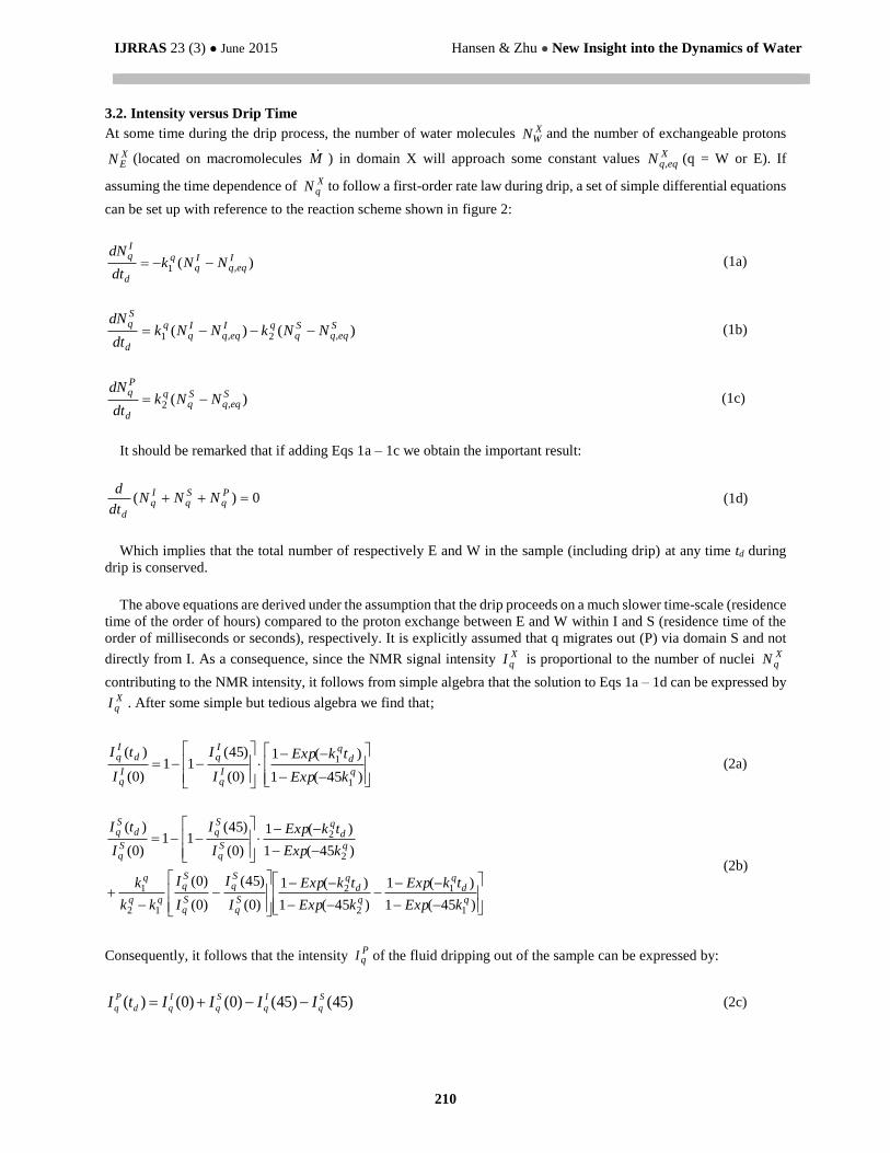
3.2. Intensity versus Drip Time

At some time during the drip process, the number of water molecules XWN and the number of exchangeable protons

XEN (located on macromolecules M ) in domain X will approach some constant values X

eqqN , (q = W or E). If

assuming the time dependence of XqN to follow a first-order rate law during drip, a set of simple differential equations

can be set up with reference to the reaction scheme shown in figure 2:

)( ,1I

eqqIq

q

d

Iq

NNkdt

dN (1a)

)()( ,2,1S

eqqSq

qIeqq

Iq

q

d

Sq

NNkNNkdt

dN (1b)

)( ,2S

eqqSq

q

d

Pq

NNkdt

dN (1c)

It should be remarked that if adding Eqs 1a – 1c we obtain the important result:

0)( Pq

Sq

Iq

d

NNNdt

d (1d)

Which implies that the total number of respectively E and W in the sample (including drip) at any time td during

drip is conserved.

The above equations are derived under the assumption that the drip proceeds on a much slower time-scale (residence

time of the order of hours) compared to the proton exchange between E and W within I and S (residence time of the

order of milliseconds or seconds), respectively. It is explicitly assumed that q migrates out (P) via domain S and not

directly from I. As a consequence, since the NMR signal intensity XqI is proportional to the number of nuclei X

qN

contributing to the NMR intensity, it follows from simple algebra that the solution to Eqs 1a – 1d can be expressed by XqI . After some simple but tedious algebra we find that;

)45(1

)(1

)0(

)45(11

)0(

)(

1

1

q

dq

Iq

Iq

Iq

dIq

kExp

tkExp

I

I

I

tI (2a)

)45(1

)(1

)45(1

)(1

)0(

)45(

)0(

)0(

)45(1

)(1

)0(

)45(11

)0(

)(

1

1

2

2

12

1

2

2

q

dq

q

dq

Sq

Sq

Sq

Sq

qq

q

q

dq

Sq

Sq

Sq

dSq

kExp

tkExp

kExp

tkExp

I

I

I

I

kk

k

kExp

tkExp

I

I

I

tI

(2b)

Consequently, it follows that the intensity PqI of the fluid dripping out of the sample can be expressed by:

)45()45()0()0()( S

q

I

q

S

q

I

qd

P

q IIIItI (2c)


211

Where )45(),0(),0( Iq

Sq

Iq III and )45(S

qI represent the proton signal intensities of q (E or W) in domains X (I, S or

P) at the start (td = 0) and at the end (td = 45 hours) of the migration process, respectively. Moreover, it follows that

the total proton signal intensity X

TI within domain X (= I and S) at any time td can be expressed by:

)()(2)( dXEd

XWd

XT tItItI (2d)

3.3. Spin-Spin Relaxation versus Drip Time

In the following section the spin-spin relaxation rate of “free” water W within any domain X is represented by

)/1( 0,2

0,2 WW TR with 0

,2 WT being the spin-spin relaxation time. Likewise, the spin-spin relaxation rate of the

exchangeable protons E located on some functional groups (for instance –COOH, –NH, –OH and –SH groups [31])

on M is denoted 0,2 ER , which is much faster than the relaxation rate of bulk water. Since various types of functional

groups on M exist, a distribution of 0,2 ER is expected. However, since it is not possible from the present NMR

measurements to derive these relaxation distribution characteristics, we simply represent them by a single, average

relaxation rate 0,2 ER .

Hence, under the condition of fast exchange between E and W, a single, observable relaxation rate XR2 for domain

X can be assigned, according to:

XWX

E

WX

XEE

XEW

XW

XXE

XW N

RR

RRNRNRNRNN

20,2

0220

,20,22)(

(3)

where all symbols are previously defined. Eq 3 shows the important result that the number of exchangeable proton

sites XEN (on M) can be calculated from the number of water molecules

X

WN by taking into account the relaxation.

This relation becomes important in the model-fitting as it reduces the number of adjustable parameters.

In particular, spin-spin relaxation time measurements is required and essential in characterizing the fate of the

exchangeable protons E during drip.

4. RESULTS AND DISCUSSION

4.1. CPMG Response Analysis

It has previously been reported that the proton CPMG response curve of meat/muscle can be well represented by a

sum of three exponential functions [33]. Using the experimental set-up shown in figure 1, we found a “3-exponential”

fit to the observed relaxation curve to give a slightly non-random error distribution, at least at longer drip times. For

instance, a typical CPMG response curve observed in this work is reproduced in figure 3a and reveals a single

exponential decay contribution, denoted D, for t 0.5 s which is characterized by a long T2 (of the order of a second)

and a small signal amplitude (~ 1 – 2 %). After subtracting ID from the observed CPMG curve, a corrected CPMG

curve is derived (figure 3b) which could be represented excellently by a sum of three exponential functions denoted

F, I and S, respectively. The excellent quality is confirmed by the random distribution of the residual curve, as

illustrated on figure 3c.

Although a model equation composed of a sum of four exponential functions may be expected to result in an ill-

posed numerical problem, we found the above procedure to be very robust for all CPMG curves analyzed in the present

work. Actually, after subtracting the fourth component (D) from the observed CMPG response function, the remaining

6 adjustable parameters - as obtained by a non-linear least-squares fit to a sum of three exponential functions - were

found to be highly reproducible. One reason for this robustness is that the four relaxation rates R2i are very different

[34] and that the signal-to-noise (S/N) ratio is high (of the order of 200 or larger). For instance, the S/N-ratio of the

CPMG curve shown in figure 3 a) was even larger (400). By arranging the relaxation rates in increasing order, each

relaxation rate was found to be faster than the former by a factor of more than 3, i.e.: DR2 ≈ 1 s-1, SR2 ≈ 9 s-1, IR2 ≈


212

25 s-1 and FR2 ≈ 900 s-1, respectively, which is fortunate. A much smaller difference between the relaxation rates

would reduce the reliability in resolving them.

0.0 0.2 0.4 0.6 0.8 1.0 1.2 1.4

1E-3

0.01

0.1

1

a)

D"Obs"

Inte

nsity

Time/s

0.00 0.25 0.501E-5

1E-4

1E-3

0.01

0.1

1

b)

Inte

nsity

Time/s

0.00 0.25 0.50

-0.002

0.000

0.002

Res

idua

l

c)

Time/s

Figure 3. a) A typical CPMG response curve of the meat sample investigated in this work. The long-T2 component D (- - -) is

excellently fitted to a single exponential function for t > 0.5 s. b) Difference between observed relaxation curve and the long-T2

component D, denoted “Corrected”, is fitted to a sum of three exponential functions F, I and S. c) Residual plot between the

“corrected” CPMG curve and the model fitted curve (3-exponential function) in b). The data shown on figure a) are taken from a

parallel experiment on an identical meat sample, using the same experimental parameters as presented in the experimental section, except for the repetition time which was set to 10 s and the number of scans which was fixed to 300.

Hence, Eq 4 is used as a model equation (or fitting function) throughout in this work in which the long-T2 component

(component D) was first fitted to a single exponential function for t > 0.5 s and then subtracted from the observed

relaxation curve before a 3-exponential fit was applied. The goodness of the above model is illustrated on figure 4 in

which the function;

ttRtIttRtI

ttRtIttRtIttI

d

D

dDd

S

dS

d

I

dId

F

dFdT

)(exp)()(exp)(

)(exp)()(exp)();(

22

22

(4)

(withDSIF RRRR 2222 ) is plotted against time t for different drip times td = 3 hours, 9 hours, 21 hours and 45

hours, respectively. The intensity ID (Eq 4) as a function of drip time will be presented in a later section in which its

physical significance will be discussed more thoroughly.


213

1.0

10.0

100.0

1 000.0

10 000.0

Inte

nsity

RI

2=22.7 s

-1R

S

2=8.2 s

-1

RF

2=840 s

-1

td=3 h

Inte

nsity

0.0 0.1 0.2 0.3 0.4 0.5

-100

0

100

Resi

dual

time (s)

Resi

dual

time (s)

time (s)

Resi

dual

1.0

10.0

100.0

1000.0

10000.0

In

tensity

td=9 h

RI

2=23.2 s

-1R

F

2=862 s

-1 RS

2=8.7 s

-1

0.0 0.1 0.2 0.3 0.4 0.5

-100

0

100

time (s)

Resi

dual

1.0

10.0

100.0

1000.0

10000.0

RI

2=27.2 s

-1

td=21 h

RF

2=867 s

-1

RI

2=25.0 s

-1 RS

2=9.3 s

-1

0.0 0.1 0.2 0.3 0.4 0.5-200

0

200

1.0

10.0

100.0

1000.0

10000.0

Inte

nsity

td=45 h

RF

2=1253 s

-1

RS

2=10.4 s

-1

0.0 0.1 0.2 0.3 0.4 0.5-200

0

200

Figure 4. CPMG relaxation curves (obtained after subtracting the long - T2 component (component D) from the observed CPMG

curve) at drip times td = 3 h, 9 h, 21 h and 45 h. The three exponential components F, I and S are shown as dotted curves in each

figure. The residual curves (the difference between observed and model calculated intensities) are shown below each figure. The red curves represent model fits to Eq 4. See text for further details.

The spin-spin relaxation rate of pure, distilled, and oxygen free water at room temperature is measured to be

approximately 0.3 – 0.4 s-1 while bulk water saturated with air/oxygen reveals a somewhat larger relaxation rate (due

to the interaction of water with paramagnetic oxygen) and amounts to between 0.6 – 1 s-1. Since the shortest of the

three proton relaxation rates in the present system is found to be larger than 8 s-1, some additional interactions or

dynamic processes must exist which dominate the relaxation of water and will be commented on in the next section.

As can be further noticed from figure 4, all residual curves reveal small, random error distributions, suggesting the

“4-exponential” relaxation model (Eq 4) to give an adequate representation of the relaxation behavior. Importantly,

these random error distributions were observed in all model-fitted relaxation curves, throughout the drip experiment.

4.2. Spin-Lattice Relaxation

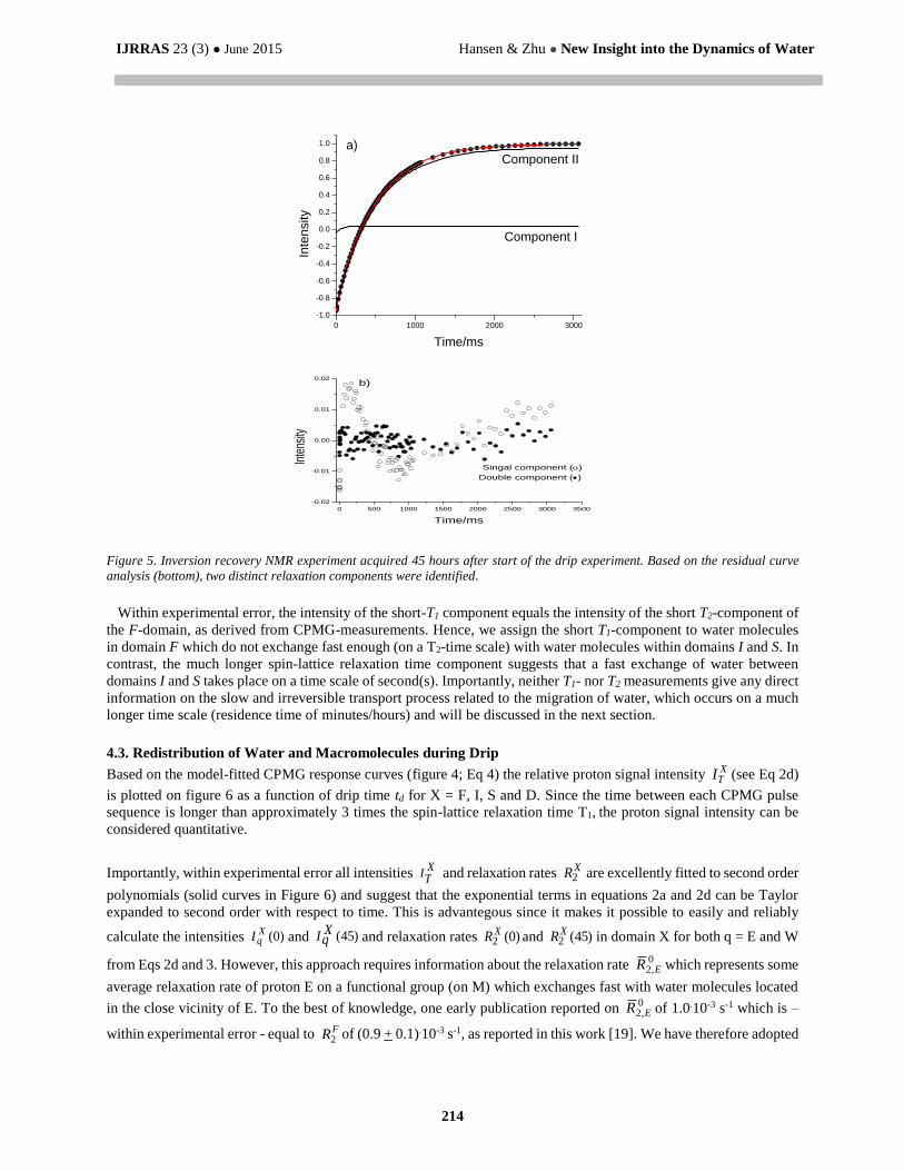
In contrast to CPMG, the Inversion Recovery measurements revealed only two distinct relaxation components; a short

relaxation component possessing a T1 = (77 + 6) ms and a relative intensity of (4.5 + 0.5)% and a second and much

longer relaxation component of T1 = (499 + 2) ms (figure 5).


214

0 1000 2000 3000

-1.0

-0.8

-0.6

-0.4

-0.2

0.0

0.2

0.4

0.6

0.8

1.0 a)Component II

Component I

Inte

nsity

Time/ms

0 500 1000 1500 2000 2500 3000 3500

-0.02

-0.01

0.00

0.01

0.02b)

Double component ()

Singal component ()

Inte

nsity

Time/ms

Figure 5. Inversion recovery NMR experiment acquired 45 hours after start of the drip experiment. Based on the residual curve

analysis (bottom), two distinct relaxation components were identified.

Within experimental error, the intensity of the short-T1 component equals the intensity of the short T2-component of

the F-domain, as derived from CPMG-measurements. Hence, we assign the short T1-component to water molecules

in domain F which do not exchange fast enough (on a T2-time scale) with water molecules within domains I and S. In

contrast, the much longer spin-lattice relaxation time component suggests that a fast exchange of water between

domains I and S takes place on a time scale of second(s). Importantly, neither T1- nor T2 measurements give any direct

information on the slow and irreversible transport process related to the migration of water, which occurs on a much

longer time scale (residence time of minutes/hours) and will be discussed in the next section.

4.3. Redistribution of Water and Macromolecules during Drip

Based on the model-fitted CPMG response curves (figure 4; Eq 4) the relative proton signal intensity XTI (see Eq 2d)

is plotted on figure 6 as a function of drip time td for X = F, I, S and D. Since the time between each CPMG pulse

sequence is longer than approximately 3 times the spin-lattice relaxation time T1, the proton signal intensity can be

considered quantitative.

Importantly, within experimental error all intensities XT

I and relaxation rates XR2 are excellently fitted to second order

polynomials (solid curves in Figure 6) and suggest that the exponential terms in equations 2a and 2d can be Taylor

expanded to second order with respect to time. This is advantegous since it makes it possible to easily and reliably

calculate the intensities )0(XqI and )45(X

qI and relaxation rates )0(2XR and )45(2

XR in domain X for both q = E and W

from Eqs 2d and 3. However, this approach requires information about the relaxation rate 0,2 ER which represents some

average relaxation rate of proton E on a functional group (on M) which exchanges fast with water molecules located

in the close vicinity of E. To the best of knowledge, one early publication reported on 0,2 ER of 1.0.10-3 s-1 which is –

within experimental error - equal to FR2 of (0.9 + 0.1).10-3 s-1, as reported in this work [19]. We have therefore adopted


215

this latter value of 0,2 ER and applied a second order polynomial fit to all data in Figure 6. The results of the analysis

are summarized in Table 1.

Figure 6. Normalized proton signal intensity of the four resolved components F, I, S (a) and D (b) as a function of drip time. The

initial sum of intensities of F, I, S and D was set to 100%. The corresponding spin-spin relaxation rates X

R2 as a function of drip

time are plotted on figure c). All solid curves represent 2. order polynomial fits and are further discussed in the text.

Within experimental error, no observable change in signal intensity or relaxation rate within domain F was noticed

(figure 6 a). In contrast, the intensity DT

I of the long-T2 component D reveals a sort of oscillating behavior with drip

time and will be commented on in a later section.

As can be inferred from the results presented in Table 1, the number of water molecules decreases by 8.5% (+ 0.1%)

in domain I and by 37% (+2%) in domain S during 45 hours of drip and truly shows the migration of water molecules

from the respective domains. This is further supported by the increase in relaxation rate of 13.1% (+ 0.3%) and 21.3%

(+ 0.3%) within the two respective domains. Also, the number of exchangeable protons in domain S decreases by

approximately 25% (+ 2%), suggesting that a significant number of macromolecules (probably smaller

macromolecules) migrate into the drip solution. This argument is based on the assumption that exchangeable protons

are associated to functional groups on the macromolecule.

a) b) c)

Time (hours) Time (hours)

Time (hours)


216

Table 1. Relative intensities )0(XqI and )45(X

qI and corresponding relaxation rates )0(2XqR and )45(2

X

qR as

calculated by second order polynomial fits to the data in Figure 6 by applying Eq 2d and 3.

Parameter Value (%)

)0(IwI 77.2 + 0.7

)45(IwI 70.6 + 0.7

)0(SwI 18.2 + 0.6

)45(SwI 11.4 + 0.6

)0(IEI 0.53 + 0.01

)45(IEI 0.60 + 0.01

)0(SEI 0.037 + 0.002

)45(SEI 0.028 + 0.002

)0(2IR 23.1 + 0.2

)45(2IR 27.2 + 0.2

)0(2SR 8.6 + 0.2

)45(2SR 9.7 + 0.2

From the present calculations we can estimate the fraction f of exchangeable protons (relative to the number of

water molecules) within any domain which extends to f = 0.015 in domain I and f = 0.004 in domain S, respectively.

From these numbers the relative ratio of macromolecules in domains I and S can be estimated to about 11. The

corresponding ratio of water molecules within the same two domains is estimated to approximately 4, showing the

density of macromolecules (macromolecule/water molecule) to be almost a factor of 3 higher in domain I than in

domain S.

One observation which seems to violate the assumption regarding irreversibility of the dynamic reaction in scheme

(Eq 1) is that the number of exchangeable protons in domain I increases with drip time by about 13% (after 45 hours

of drip). We do not have a clear understanding of this result. However, we may speculate about it and we find two

reasonable justifications:

1. Some small macromolecules (or acid protons) may diffuse from domain F and into domain I during drip. This

net migration would not significantly affect the relaxation rate or proton signal intensity in domain F which is

expected to possess a pool of macromolecules with a higher concentration of macromolecules compared to

domains I and S. In contrast, a small amount of macromolecules migrating from F and into I may significantly

affect the number of macromolecules in I. A potential migration of macromolecules and/or water from F is not

implemented in the dynamic reaction model (scheme 1).

2. The accessibility of exchangeable protons on M may change during drip due to restructuring of the

macromolecules - for instance by denaturation [13,36] and may affect the number XEN .

Finally, we address the question of molecular dynamics or migration, i.e., the rate of change of E and W during

drip. This can simply be resolved by fitting Eqs 2a, 2b, 2d and 3 to the observed intensity/relaxation curves in Figure

6. All parameters, except the rate constants, are known (Table 1) and leave only four (4) parameters adjustable for

model fitting. The model fitted relaxation curves and intensities are shown in Figure 6 and – not surprisingly –

coincide with the 2.order polynomial fits, as mentioned previously. The rate constants are summarized in Table 2.


217

Table 2. Rate constants Wk1 , Wk2 , Ek1 and Ek2 as determined by a simultaneous fit of Eqs 2a, 2b, 2d and 3 to the

data in Figure 6. All parameters except the rate constants were kept fixed (Table 1). The respective errors in the

rate constants were estimated by Monte Carlo simulations in which the non-adjustable parameters (Table 1) were

chosen randomly (from a normal distribution) before each model fit.

Rate constant Value

Wk1 (1.7 + 0.8).10-6 s-1

Wk2 (7.5 + 0.2).10-6 s-1

Ek1 (3 + ).10-8 s-1

Ek2 (1 + ).10-6 s-1

The analysis demonstrates that neither Ek1 nor Ek2 could be reliably determined which is most probably caused by

their rather small intensities of less than 2%.

In contrast, the rate constant for the migration of water from domain S was found to be approximately 4 – 5 times

faster than the migration of water from domain I. This is not unexpected, as the migration of water from domain I is

motionally more constraint, as it contains a larger concentration of macromolecules (macromolecules/water molecule)

compared to domain S. As a consequence, the drip is strongly governed by migration of water from domain S while

the migration from I probably comes into play at a later stage during drip. If assigning I and S to the inter/intra- and

extramyofibrillar space, respectively [17] the reduced intensity at longer drip time may be explained by myofibrillar

shrinkage and longitudinal contraction which “forces” free water from I and subsequently into S, and subsequently

out into P, i.e., resulting in a net loss of water from both domains I and S. Such a shrinkage effect can be argued from

the XR2 -behavior with time, as it is well known that XR2 is proportional to the surface-to-volume ratio (S/V) of domain

X. For spherical or cylindrical geometries it thus follows that the inverse of the diameter or the inverse length of a

cylinder becomes proportional to the water relaxation rate XR2 . Hence, according to the relaxation data presented in

figure 6 (right) the diameter/length of the domain (I and/or S) would decrease by 10 – 15% during 45 hours of drip

resulting in a subsequent "collapse" (volume reduction) of the domain X as drip progresses. To the best of knowledge,

this was first suggested by Bertram and colleagues [15].

4.4. “Drip” - curve

By applying Eq 4 the drip-loss can be calculated by subtracting the overall observed signal intensity IT(td) from the

initial signal intensity IT(0) and is shown by open circles (o) on figure 7 a in which the solid curve was calculated by

a simple second order polynomial fit. The difference between the observed and fitted drip curves is illustrated on

figure 7 b by open circles (o).

0 10 20 30 40 500

5

10

15

td/hour

Inte

nsity (

%)

a)

0 10 20 30 40 500,0

0,4

0,8

1,2

1,6

2,0

Inte

nsity (

%)

td/hour

b)

Figure 7. a) Observed drip curve (o) in meat as a function of drip time td. The solid curve (──) represents a simple 2.order

polynomial fit. b) Difference between observed and model-fitted intensities from Figure a). The solid points (●) are reproduced

from figure 6 (right).


218

As can be inferred from the data in Figure 7b, the “oscillating” behavior of the drip curve - as illustrated by the

open circles (o) in Figure 7 a – resembles the behavior the corresponding oscillation behavior of the long-T2 component

D (●) and leads to the tentative conclusion that the overall drip-curve is composed of two compoments. One

component which increases monotonically with time (main drip) and a second small-amplitude, oscillating component,

denoted “residual drip” which is tentatively believed to build up on the outer surface of the sample. Probably, small

water drops evaporated and condensed (or adhered) to the inner glass wall of the NMR tube and water confined at the

sample surface. As time progresses, this water then drips (flows) out from the detector coil. However, the oscillating

behavior continuous as long as the main drip component forms. Actually, we have seen this phenomenon on all drip

experiments performed on our small sample NMR instrument. This topic is under further investigation in our

laboratory and will be discussed elsewhere.

4.5. Spin-Spin Relaxation Time Characteristics of the Drip-Fluid

Although it is known that macromolecules (proteins) migrate out and into the drip solution with time [37] we will in

this last section give support for this statement by spin-spin relaxation time measurements performed on the drip

solution. According to Cooke et al. [38], the relaxation mechanisms in muscle fibers and protein solutions (here drip

solution) are similar. Actually, to obtain a reliable fit of the observed relaxation curve of the drip fluid, it was necessary

to adopt three individual relaxation components, as illustrated on the CPMG response curve of the drip fluid in figure

8 and by the results presented in Table 3, of which one component has an R2 component comparable to bulk water.

The other two components show much larger relaxation rates and are of the same order of magnitude as in the meat

sample (see figure 4). The observation of three distinct components in the drip fluid suggests that the various proton

species are not satisfying the fast exchange conditions.

0 2 4 6 8 1010

100

1000

a)

Inte

nsity (

a.u

.)

Time (s)

Figure 8. a) CPMG response of the drip fluid after 45 hours drip. b) Residual. The experimental parameters were the same as

presented in the experimental section, except for the repetition time which was set to 15 s, = 0.5 ms and the number of

transients N = 16.

Hence, the above relaxation time measurements simply support previous results that macromolecules migrate from

the meat and into the drip solution. It is reasonable to expect that T2 of the drip solution will change with drip time.

However, this topic is not part of the present work and will not be discussed further.

0 2 4 6 8 10

-200

0

200

Res

idua

l

Time/s

b)


219

Table 3. Spin-spin relaxation rate R2 within the drip solution (after 45 hours of drip)

derived by a“3-exponential” fit to the observed relaxation response function in figure 8.

Component R2

(s-1)

Intensity

(%)

1 23.7 + 0.3 69.9 + 0.8

2 6.2 + 0.3 11.1 + 0.1

3 0.452 + 0.002 19.0 + 0.1

6. SUMMARY AND CONCLUSION In this work we have reported proton CPMG experiments performed on porcine longissimus dorsi muscle samples

(8ϕ x 10 mm, ~0.459 g) during drip which enables three dynamic domains X (= F, I and S) to be identified and their

proton signal intensity XTI and spin-spin relaxation rate XR2 to be monitored as a function of time. A monotonic

increase/decrease in XR2 /IX was noticed within all domains, except for the F-domain, which intensity and relaxation

rate remained – within experimental error - constant during drip.

Meat/muscle is a rather heterogeneous and complex biological material containing macromolecules that are most

probably described by a broad distribution of molar masses and possessing a corresponding distribution regarding the

number of (water) adsorption sites per macromolecule.

It is further known that water molecules that interact with exchangeable protons on a macromolecule possess a

faster spin-spin relaxation rate R2 [38]. The existence of such relaxation sink sites are particularly important in

biological materials and may significantly affect the relaxation rate.

It is thus necessary to make some model simplifications/assumptions in order to gain some relevant

physical/chemical insight from the observed NMR intensity- and relaxation data. Hence, a simple first-order kinetic

model was designed which solutions (Eqs 2 and 3) were fitted simultaneously to the observed NMR signal

intensities/relaxation rates of domains I and S and enabled the rate constant for the migration of water between

domains to be established.

A) The total number of protons within any domain X (= F, I and S) is expressed by the sum of exchangeable

protons XEN on a macromolecule and free water molecules X

WN . The exchange rate of these water

molecules is a fast process (characterized by a short residence time of the order of a few ms) as compared

to the irreversible transport or migration process , i.e. drip-loss, which is a slow process, characterized

by long residence time of the order of hours).

B) The probability of water molecules W to exchange with exchangeable protons E on a macromolecule

will depend on the population of both E and W, which may change during the migration process. Also,

restructuring of the macromolecules may affect the number of E (for instance by denaturation [13,36]).

C) A contraction or shrinkage of a domain X may lead to an extra “push” of water molecules out of that

domain and results in a relative enhancement of the fraction of adsorbed water molecules remaining. As a

consequence, the spin-spin relaxation rate R2 will increase (due to the fast exchange of free and bonded water

molecules within the domain) and enables the S/V-ratio of the domain to be estimated.

Options A – B rationalize all the findings presented in this work, including the slow migration or drip of

macromolecules.

Finally, we will emphasize that due to the rather small fraction of exchangeable protons (< 2% of the total proton

intensity), it was not possible to obtain any reliable estimate of the migration rate of the macromolecules.


220

7. ACKNOWLEDGEMENTS We want to thank the Research Council of Norway for financial support through the project “On line determination

of water retaining ability in pork muscle”, Project number 229192 and the project INFORMED (Increased

Efficiency: Moving from Assumed Quality to Online Measurement and Process, Nortura SA, Project no.: 210516).

Also, we are grateful for reviews from Prof. Bjørg Egelandsdal at Norwegian University of Life Sciences and

director Per Berg at Nortura during the preparation of the manuscript.

8. REFERENCES

[1]. O.R. Fennema, J. Muscle. Foods. 1, 363-381 (1990)

[2]. A. Schäfer, K. Rosenvold, P.P. Purslow, H.J. Andersen, P. Henckel, Meat Sci. 61, 355–366 (2002)

[3]. C.J. Walukonis, M.T. Morgan, D.E. Gerrard, J.C. Forrest, A Technique for Predicting Water-Holding Capacity

in Early Postmortem Muscle. (Purdue University 2002 swine research report, 2002),

http://www.ansc.purdue.edu/swine/swineday/sday02/18.htm. Accessed 10 December 2013

[4]. M. Prevolnik, M. Čandek-Potokar, D. Škorjanc, J. Food Eng. 98, 347–352 (2010)

[5]. A.J. Rasmussen, M. Andersson, 42nd. International Congress of Meat Science and Technology, 1996

[6]. G. Offer, T. Cousins, J. Sci. Food. Agric. 58, 107-116 (1992)

[7]. M.J.D. Hertog-Meischke, R.J. Van Laack, F.J. Smulders, Vet Quart. 19, 175-181 (1997)

[8]. R.G. Kauffman, in Meat Science and Applications, ed. By Y.H. Hui, W.K. Nip, R. Rogers, (CRC Press: New

York, 2001), p.1

[9]. K.L. Pearce, K. Rosenvold, H.J. Andersen, D.L. Hopkins, Meat Sci. 89, 111–124 (2011)

[10]. E. Gjerlaug-Enger, Genetic Analyses of Meat, Fat and Carcass Quality Traits Measured by Rapid Methods.

Phd thesis, Norwegian University of Life Science, 2011.

[11]. H.C. Bertram, A.H. Karlsson, M. Rasmussen, O.D. Pedersen, S. Dønstrup, H.J. Andersen, J. Agr. Food. Chem.

49, 3092-3100 (2001)

[12]. E. Tornberg, M. Wahlgren, J. Brøndum, S.B. Engelsen, Food. Chem. 69, 407-418 (2000)

[13]. H.C. Bertram, H.J. Andersen, Ann. R. NMR. S. 53, 157–202(2004)

[14]. J.P. Renou, G. Monin, P. Sellier, Meat Sci. 15, 225-233 (1985)

[15]. H.C. Bertram, P.P Purslow, H.J. Andersen, J. Agr. Food. Chem. 50, 824–829 (2002)

[16]. P.S. Belton, K.J. Packer, Biochim. Biophys. Acta. 354, 305–314 (1974)

[17]. H.C. Bertram, A. Schäfer, K. Rosenvold, H.J. Andersen, Meat Sci. 66, 915–924 (2004)

[18]. R.T. Pearson, W. Derbyshire, J.M.V. Blanshard, Biochem. Bioph. Res. Co. 48, 873-879 (1972)

[19]. W.T. Sobol, I.G. Cameron, W.R. Inch, M.M. Pintar, Biophys. J. 50, 181-191 (1986)

[20]. C.F. Hazlewood, D.C. Chang, B.L. Nichols, D.E. Woessner, Biophys. J. 14, 583-606 (1974)

[21]. G. Favetto, J. Chirife, G.B. Bartholomai, J. Food. Technol. 16, 621-628 (1981)

[22]. A. Kondjoyan, A. Kohler, C.E. Realini, S. Portanguen, R. Kowalski, S. Clerjon, P. Gatellier, S. Chevolleau,

J.M. Bonny, L. Debrauwer, Meat Sci. (2013) doi: 10.1016/j.meatsci.2013.07.032

[23]. M. Chabbouh, S.B.H. Ahmed, A. Farhat, A. Sahli, S. Bellagha, Food. Bioprocess. Tech. 5, 1882–1895 (2012)

[24]. G. Sartor, G.P. Johari, J. Phys. Chem, 100, 1045-1046 (1996)

[25]. B.E. Elizalde, A.M.R. Pilosof, L. Dimier, G.B. Bartholomai, J. Am. Oil. Chem. Soc. 64, 1454-1458 (1989)

[26]. I. Muñoz, N. Garcia-Gil, J. Arnau, P. Gou, Meat. J. Food. Eng. 110, 465–471 (2012)

[27]. E.E. Burnell, M.E. Clark, J.A. Hinke, N.R. Chapman, Biophys. J. 33, 1–26 (1981)

[28]. S. Meiboom, D. Gill, Rev. Sci. Instrum. 29, 688-691 (1958)

[29]. B.M. Fung, P.S. Puon, Biophys. J. 33, 27–37 (1981)

[30]. P.J. Lattanzio, K.W. Marshall, A.Z. Damyanovich, H. Peemoeller, Magnet. Reson. Med. 44, 840–851 (2000)

[31]. C.K. McDonnell, P. Allen, E. Duggan, J.M. Arimi, E. Casey, J. Duane, J.G. Lyng, Meat Sci. 95, 51–58 (2013)

[32]. J.R. Zimmerman, W.E. Brittin, T. J. Phys. Chem. 61, 1328-1333 (1957)

[33]. W.C. Cole, A.D. LeBlanc, S.G. Jhingran, Magnet. Reson. Med. 29, 19-24 (1993)

[34]. M. Nilsson, M. A. Connell, A. L. Davies and G. A. Morris. Anal. Chem. 78, 3040 – 3045 (2006)

[35]. M.J.A.D. Hertog-Meischke, F.J.M. Smulderst, J.G.V. Logtestijn, J. Sci. Food. Agr. 78, 522-526 (1998)

[36]. M.J.A.D. Hertog-Meischke, R.E. Klont, F.J.M. Smulders, J.G.V. Logtestijn, Meat. Sci. 47, 323-329 (1997)

[37]. A.W.J. Savage, P.D. Warriss, P.D. Jolley, Meat. Sci. 27, 289–303 (1990)

[38]. N. Bloembergen, E.M. Purcell, R.V. Pound, Phys. Rev. 73, 679-712 (1948)

new insight into the dynamics of water and macromolecules ... · pdf filenew insight into the...

Documents