1

New Insights from a Fixed Point Analysis ofSingle Cell IEEE 802.11 WLANs∗

Anurag Kumar1, Eitan Altman2, Daniele Miorandi3 and Munish Goyal1

Abstract— We study a fixed point formalisation of the wellknown analysis of Bianchi [3]. We provide a significant simpli-fication and generalisation of the analysis. In this more generalframework, the fixed point solution and performance measuresresulting from it are studied. Uniqueness of the fixed point is es-tablished. Simple and general throughput formulas are provided.It is shown that the throughput of any flow will be boundedby the one with the smallest transmission rate. The aggregatethroughput is bounded by the reciprocal of the harmonic meanof the transmission rates. In an asymptotic regime with a largenumber of nodes, explicit formulas for the collision probability,the aggregate attempt rate and the aggregate throughput areprovided. The results from the analysis are compared with ns2simulations, and also with an exact Markov model of the back-off process. It is shown how the saturated network analysis canbe used to obtain TCP transfer throughputs in some cases.

Keywords: wireless networks, CSMA/CA, performanceof MAC protocols

I. INTRODUCTION

We are concerned in this paper with the situation in whichthere are several IEEE 802.11 compliant nodes within sucha distance of each other that only one transmission can besustained at any point of time. We call these single-cellnetworks. Our discussion covers ad hoc networks, and alsoinfrastructure networks, in which an AP acts as a conduitbetween the wireless network and a wired “infrastructure.”Our analysis is limited to the situation in which all nodes usethe RTS/CTS based distributed coordination function (DCF)without the QoS extensions (as in IEEE 802.11e) (but see [9]for our extensions of the work in the present paper).

Each node may have several physical connections or asso-ciations with several other nodes. On each such connectionthe sustainable physical transmission rate may be different.Between each such pair of nodes there are flows whosethroughput performance we are concerned with. It is assumedthroughout this paper that all flows are infinitely back-loggedat their transmitters; i.e., there are always packets to transmitwhen a node gets a chance to do so.

∗To appear in IEEE Transactions on Networking. This is an extendedversion of a paper that appeared in IEEE Infocom 2005. The research wassupported by the Indo-French Centre for Promotion of Advanced Research(IFCPAR) under research contract No. 2900-IT. c©2006 IEEE. Personal useof this material is permitted. However, permission to reprint/republish thismaterial for advertising or promotional purposes or for creating new collectiveworks for resale or redistribution to servers or lists, or to reuse any copyrightedcomponent of this work in other works, must be obtained from the IEEE.

1ECE Department, Indian Institute of Science, Bangalore, INDIA; email:anurag, munish@ece.iisc.ernet.in

2INRIA, Sophia-Antipolis, FRANCE; email: Eitan.Altman@sophia.inria.fr3CREATE-NET, Trento, Italy; email: daniele.miorandi@create-net.org

In such a scenario, we are interested in obtaining quantita-tive formulas and qualitative insights via a stochastic analysisof the way that the IEEE 802.11 CSMA/CA protocol allocatesthe wireless medium to the node transmitters. Our approachis to begin with a key approximation made by Bianchi [3].This leads to a fixed point equation, which can be expected tocharacterise the operating points of the system. This fixed pointequation is our point of departure. We simplify and generalisethe analysis leading to the fixed point equation. We thenestablish a simple, and practically appealing, condition for theuniqueness of the fixed point in this more general framework.Some simple observations lead to throughput formulas for theoverall network and for the individual flows. These formulasallow us to recover the well known observation that the slowesttransmission rate dominates the throughput performance. Wealso analyse the fixed point in the asymptotic regime of alarge number of nodes and find explicit formulas for thecollision probability, the channel access rate and the networkthroughput. A key parameter in the protocol is the back-offmultiplier, whose default value in the IEEE 802.11 MACstandard is 2; our asymptotic analysis provides some insightsinto the role of the back-off multiplier.

We provide ns2 simulation results for the collision proba-bilities and compare these with results obtained from the fixedpoint analysis. We also provide results from an exact Markovchain model for the back-off process and also compare theseresults with those from the fixed point analysis.

As already pointed out, the above described modelingassumes that there are always packets backlogged on everyconnection. Such a saturation assumption is a common simpli-fication and is useful in the following ways. In some situationsit has been formally proved (see, for example, [1] and [6]) thatthe saturation throughput provides a sufficient condition forstability of the queues; i.e., if at each queue the arrival rate isless than the saturation throughput then the queues will have aproper, joint stationary distribution. In this paper we also applythe saturation throughput analysis to provide an analysis forTCP controlled file transfer throughputs in certain local areanetwork scenarios.

The most popular model for IEEE 802.11 networks, and onethat has led to many applications and extensions, is the onereported in [3]. Another analysis, that also incorporates thefeature of adapting the back-off parameters, has been reportedin [4]. The recent paper [2] is one of the many that havereported a throughput “anomaly” in IEEE 802.11 networks;i.e., if the network has low speed connections, even the highspeed connections experience throughput no better than whatis obtained by the low speed connections.

2

The paper is organised as follows. In Sec. II we providethe key observation and approximation on which the analysisis based. In Sec. III we analyse the back-off process in afairly general setting. The fixed-point equation is provided inSec. IV and analysed in Sec. V; a validation through an exactsolution of a Markov model is given in Sec. V-B. In Sec. VIthe throughput formulas are provided. The asymptotic analysisis developed in Sec. VII. An application of the results to theanalysis of TCP is given in Sec. VIII and the paper ends witha concluding section. Some proofs are provided in-line andothers are in the Appendix. Some details, not provided in thispaper (including the proof of Theorem 5.2), can be found inthe technical report [5].

II. A KEY OBSERVATION AND AN APPROXIMATION

A. Sufficiency of the Analysis of the Back-Off ProcessWe begin by extracting from a description of the system

the key modeling abstractions that will allow us to developthe analysis. Figure 1 shows the evolution of the systemfor 4 nodes; shown are the back-offs, the transmissions andcollisions. In the IEEE 802.11 standard, the back-off durationsare in multiples of a standardised time interval called a slot(e.g., 20 µs in IEEE 802.11b). However, this discrete natureof the back-offs does not affect the following argument. Whena node completes its back-off (for example, node 1 is the firstto complete its back-off in Figure 1), it seeks a reservationof the channel by sending an RTS packet. If no other nodecompletes its back-off before hearing this transmission thenthe RTS effectively reserves the channel for the first node.There follows a CTS from the intended recipient of the RTS,and then there follows a packet transmission and a MAClevel ACK. This ends the reservation period and the node thattransmitted the packet samples a new back-off interval. Notethat we assume throughout that nodes always have packets totransmit; i.e., all the transmission queues are saturated.

If the RTS collides with that of another node (note thatwe do not model the phenomenon of packet capture), thenafter fully transmitting their RTSs each transmitting node waitsfor a time interval SIFS + TCTS +DIFS, where TCTS isthe time required to transmit a CTS (at the control rate of2 Mbps), before returning to the back-off state. For example,in Figure 1 nodes 2 and 4 collide after the first two attempts (bynodes 1 and 3, respectively) are successful. The other nodes,not involved in the collision, and not being able to decodeanything, listen to the channel activity until the end of theRTS transmissions, and then wait for an amount of time equalto EIFS (= SIFS + TACK + DIFS). Since an ACK and aCTS have the same number of bits, after a collision all nodesresume their back-off phases after an amount of time equal tothe transmission time of an RTS plus a fixed time (equal ineach case to an EIFS).

If attempts to send the packet at the head-of-the-line (HOL)meet with several successive failures, this packet is discarded.By our assumption of saturated queues, there is always anotherpacket waiting to be sent by the upper layers: either the samepacket or the next one in line.

We see from the figure that when any node has reserved thechannel or whenever there is a collision, all other nodes freeze

their back-off timers. We also notice that the evolution of thechannel activity after an attempt is deterministic. It is eitherthe time taken for a transmission or for a collision. If there isa transmission then the time depends on which node capturesthe channel. The latter dependence comes about because thetransmission time of a packet depends on the transmission rateand hence on the transmitting node.

Since all nodes freeze their back-offs during channel activ-ity, the total time spent in back-off up to any time t, is thesame for every node. With this observation, let us now lookat Figure 2 which shows the back-offs of Figure 1 with thechannel activity removed. Thus in this picture “time” is justthe cumulative back-off time at each node. In the IEEE 802.11standard the back-offs are multiples of the slot time. A successoccurs if a single back-off ends at a slot boundary, and acollision occurs when two or more back-offs end at a slotboundary. The nodes could have different back-off parameters(the mean back-off intervals, how these are varied in responseto collisions and successes, and the number of retries of apacket). It is clear, however, that the (random) sequence inwhich the nodes seek turns to access the channel and whetheror not each such attempt succeeds depends only on the back-off process shown in Figure 2. It is therefore sufficient toanalyse the back-off process in order to understand the channelallocation process. The saturation assumption is crucial heresince, with this assumption, we do not have to take care of anyexternal packet arrivals that may occur during channel activityperiods.

Thus, in summary, we can delete the channel activityperiods, and we are left with a “conditional time” which wewill call back-off time. We will analyse the back-off processconditioned on being in back-off time. It will then be shownhow this analysis can be used to yield the desired performancemeasures over all time.

B. A Key Approximation

Throughout the rest of the paper we assume that all thenodes use the same back-off parameters. Hence the back-off process shown in Figure 2 is symmetric over the nodes.We call this the homogeneous case to distinguish it fromthe nonhomogeneous case in which different nodes may usedifferent back-off parameters, as, for example, proposed in theIEEE 802.11e standard (see [8] and [9]).

In Figure 2 we also show the aggregate sequence of suc-cesses and collisions. In general, this is a complex process, andit is also clear that the success and collision processes of thevarious nodes are coupled and strongly correlated. In Sec. V-Bwe will describe an exact Markov chain model for the jointbackoff process of the nodes, but this model is analyticallyintractable. The following key approximation is made in [3].The Decoupling Approximation: Let β denote the long runaverage back-off rate (in back-off time) for each node. Bythe fact that all nodes use the same back-off parameters,and by symmetry, it is assumed that all nodes achieve thesame value of β. Let there be n contending transmitters,and consider a given node. The decoupling approximationis to assume that the aggregate attempt process of the other

3

��������������������������������

����������������������������������������������������

������������������������������������������������������������������������������

����������������������������������������������������

������������

����������������������������

� � � � � � � � � � � � � � ��������������������������������������������������������������������������

����������������������������

������������

������������������

�������������������������������� ���������������������������������������������������� ��������������

�������������� ������������������������������������������������������������

��������������������������������������������� � � � � � � � � � � � � � � � � � � � � �

!�!�!�!�!!�!�!�!�!"�"�"�""�"�"�"

#�#�#�#�##�#�#�#�##�#�#�#�#$�$�$�$$�$�$�$$�$�$�$

%�%�%�%%�%�%�%%�%�%�%&�&�&�&&�&�&�&&�&�&�&

'�'�'�'�'�'�'�''�'�'�'�'�'�'�'(�(�(�(�(�(�(�((�(�(�(�(�(�(�(

)�)�)�))�)�)�))�)�)�)*�*�**�*�**�*�*

+�++�++�+,�,,�,,�,-�--�-.�..�.

/�//�/0�00�0

1�11�12�22�2

3�3�3�3�3�3�33�3�3�3�3�3�34�4�4�4�4�44�4�4�4�4�4 5�5�5�5�5�55�5�5�5�5�56�6�6�6�6�66�6�6�6�6�67�7�7�7�7�77�7�7�7�7�78�8�8�8�8�88�8�8�8�8�8

9�9�99�9�99�9�9:�:�::�:�::�:�:

1

2

3

4

node

successive backoffssuccessful transmissioncollision

Fig. 1. The evolution of the back-off periods and channel activityfor four nodes. Back-offs are interrupted by channel activity, i.e., packettransmissions and RTS collisions.

;<;<;<;;<;<;<;;<;<;<;=<=<=<==<=<=<==<=<=<=

><><><>><><><>?<?<?<??<?<?<?

@<@<@<@@<@<@<@A<A<A<AA<A<A<A

B<B<B<BB<B<B<BB<B<B<BC<C<C<CC<C<C<CC<C<C<C

D<D<D<D<D<D<DD<D<D<D<D<D<DE<E<E<E<E<E<EE<E<E<E<E<E<E F<F<F<FF<F<F<FG<G<G<GG<G<G<GH<H<H<H<H<H<H<H<HH<H<H<H<H<H<H<H<HI<I<I<I<I<I<I<II<I<I<I<I<I<I<I

J<J<J<J<J<J<JJ<J<J<J<J<J<JJ<J<J<J<J<J<JK<K<K<K<K<K<KK<K<K<K<K<K<KK<K<K<K<K<K<K

L<L<L<LL<L<L<LL<L<L<LM<M<M<MM<M<M<MM<M<M<M

N<N<N<N<N<N<N<N<NN<N<N<N<N<N<N<N<NN<N<N<N<N<N<N<N<NO<O<O<O<O<O<O<OO<O<O<O<O<O<O<OO<O<O<O<O<O<O<O

P<P<P<P<P<P<PP<P<P<P<P<P<PP<P<P<P<P<P<PQ<Q<Q<Q<Q<Q<QQ<Q<Q<Q<Q<Q<QQ<Q<Q<Q<Q<Q<Q

R<R<R<RR<R<R<RR<R<R<RS<S<S<SS<S<S<SS<S<S<S

T<T<T<T<T<T<T<T<TT<T<T<T<T<T<T<T<TT<T<T<T<T<T<T<T<TU<U<U<U<U<U<U<UU<U<U<U<U<U<U<UU<U<U<U<U<U<U<U

V<V<V<V<V<V<VV<V<V<V<V<V<VW<W<W<W<W<W<WW<W<W<W<W<W<W X<X<X<XX<X<X<XY<Y<Y<YY<Y<Y<YZ<Z<Z<Z<Z<Z<Z<Z<ZZ<Z<Z<Z<Z<Z<Z<Z<Z[<[<[<[<[<[<[<[[<[<[<[<[<[<[<[

\<\<\\<\<\]<]<]]<]<]

^<^<^^<^<^^<^<^_<_<__<_<__<_<_

`<`<``<`<``<`<`a<a<aa<a<aa<a<a

b<b<bb<b<bc<c<cc<c<c

x x x x

1

2

3

4

node

attemptprocess

aggregate collision

successes

Fig. 2. After removing the channel activity from Figure 1 only the back-offs remain. At the bottom is shown the aggregate attempt process on thechannel, with three successes and one collision.

(n − 1) nodes is independent of the back-off process of thegiven node. In IEEE 802.11 the back-off evolves over slots,hence a discrete time model (embedded at slot boundaries)can be adopted. Then the approximation is the following:(i) The “influence” of the other nodes on a tagged node ismodeled via the decoupling approximation. Attempts by atagged node over slots experience the collision probabilityγ. For a given collision probability this yields one equationβ = G(γ) (see Eqn. 1); (ii) The nodes are assumed to attemptin each slot with a constant (state independent) probabilityequal to the average attempt rate, β. Then, conditional on atagged node attempting, the number of attempts by other nodesis binomially distributed. This yields the other (“coupling”)equation γ = Γ(β) (see Eqn. 2). When these equations are puttogether we obtain the desired fixed point equation. It might beexpected that such a decoupling approximation should workwell when there is a large number of transmitters accessingthe channel.

III. ANALYSIS OF THE BACK-OFF PROCESS

We generalise the back-off behaviour of the nodes, anddefine the following back-off parameters.

K := At the (K + 1)th attempt either the packet succeedsor is discarded

bk := The mean back-off duration (in slots) at the kthattempt for a packet, 0 ≤ k ≤ K

Since we are limiting ourselves to the homogeneous case, theseparameters are the same for all the nodes.

In Figure 3 we show the evolution of the back-off processfor a single node. There are Rj attempts until success for thejth packet (no case of a discarded packet is shown in thisdiagram), and the sequence of back-offs for the jth packetis B

(i)j , 0 ≤ i ≤ Rj − 1. Thus the total back-off for the jth

packet is given by Xj =∑Rj−1

i=0 B(i)j with E

(

B(i)j

)

= bi. Weobserve that the sequence Xj , j ≥ 1, are renewal life times.Hence, viewing the number of attempts Rj for the jth packetas a “reward” associated with the renewal cycle of length Xj ,we obtain from the renewal reward theorem that the back-off rate is given by E(R)/E(X). Now let γ be the collisionprobability seen by a node, i.e.,

γ := Pr (an attempt by a node fails because of a collision)

Since the back-off behaviour of all the nodes is the same,the collision probability is the same for all the nodes. By theapproximation made in Sec. II, the successive collision eventsare independent. It is then easily seen that

E(R) = 1 + γ + γ2 + · · · + γK

E(X) = b0 + γb1 + γ2b2 + · · · + γkbk + · · · + γKbK

which yields the following formula for the attempt rate for agiven collision probability γ

G(γ) :=1 + γ + γ2 + · · · + γK

b0 + γb1 + γ2b2 + · · · + γkbk + · · · + γKbK

(1)

Note that, since the back-off times are in slots, the attemptrate G(γ) is in attempts per slot.

Remarks 3.1:1) Note that the distribution of the back-off durations doesnot matter. Also, observe that the above analysis remainsunchanged whether the back-off distributions are discrete (i.e.,the back-offs evolve over slots) or are continuous.2) In the back-off model considered in [3] K = ∞; further,there is an m ≥ 1 such that bk =

(

2kCWmin±12

)

slots, for

0 ≤ k ≤ m − 1, and bk =(

2mCWmin±12

)

slots, for k ≥ m.Here CWmin is a positive integer (25 in the IEEE 802.11standard). Substituting these into the expression for G(γ) inEquation 1 yields

G(γ) =2(1 − 2γ)

(1 − 2γ)(CWmin ± 1) + γCWmin(1 − (2γ)m)

attempts per slot, which is the same as in the paper [3]. Notethat the ± alternatives arise depending on whether we takethe back-off to be uniformly distributed over [1, 2, · · · , CW ]or over [0, 1, · · · , CW −1]. Evidently, the uniform distributionof back-off durations plays no role in the final results in [3].3) A more detailed evolution of the back-off process inFigure 3 is shown in Figure 4, where at each time t theresidual back-off duration Y (t) is also shown. The processZ(t) is the back-off stage the node is in. Thus if K = 7,Z(t) = 3, and Y (t) = 5, then after 5 time units the currentback-off ends. If there is a collision, Z(t) changes to 4 and

4

B B B B B B B B B B0 0 0 0 011 12 31 1 2 3 3 4 5 5

collisions

successes

X X X X X1 2 3 4 5

R = 2 R = 1 R = 4 R = 11 2 3 54 R = 2

3 3

Fig. 3. Evolution of the back-offs of a node. Each attempted packet starts anew back-off “cycle.”

back−offstage

X X X X X1 2 3 4 5

Y(t): residual back−off process

Z(t) 0 1 0 0 1 2 3 0 0 1

Fig. 4. Evolution of the back-off stage (Z(t)) and the residual back-offtime (Y (t)) for the case in which the back-offs are continuous variables.

a back-off with mean b4 is sampled from the specified back-off distribution (uniform in the standard). If Z(t) = 7 then atthe end of the current back-off, irrespective of whether thereis a collision or a success, the next back-off has mean b0,and is sampled from the specified distribution. It is clear thatthe process (Z(t), Y (t)) is Markov. The point is that it is notnecessary to analyse this Markov chain, which is essentiallywhat is done in [3]. Let Zk, k ≥ 0, denote the process Z(t)embedded at the attempt instants (the instants correspondingto the vertical sides of the triangles in Figure 4). Then Zk is anembedded Markov chain. Further, Zk and the successive back-off intervals (the bases of the triangles) constitute a Markovrenewal process. It is well known that for Markov renewalprocesses event rates and time probabilities are insensitive todistributions of life-times. It should thus be clear why onecan directly obtain the formulas above without needing to gothrough the analysis of the Markov chain in [3], and also whythe results are insensitive to the back-off distribution.

IV. THE FIXED POINT EQUATION

Focusing on the back-off and attempt process of a node,and being given the collision probability γ the attempt rateis provided by G(γ) in Eqn. 1. It is important to recall thatin the present discussion all rates are conditioned on being inthe back-off periods. Later we will see how to incorporate thechannel activity periods. Now if all nodes have the same back-off parameters, they will all see the same average collisionprobability, γ, and hence will have the same attempt rate.If the attempt rate (or probability) of each node per slot isβ, 0 ≤ β ≤ 1, then, conditioning on an attempt of the givennode, the probability of this attempt experiencing a collisionis the probability that any of the other nodes attempts in thesame slot. Under the decoupling approximation, the numberof attempts made by the other nodes is binomially distributedwith parameters β and n − 1. Under the approximation, thenumber of attempts in successive slots form an i.i.d. sequence.The probability of collision of an attempt by a node is givenby

Γ(β) := 1 − (1 − β)(n−1) (2)

We will show later in the paper that under a certain asymptoticregime the aggregate attempt rate nβ converges to a positivevalue as n → ∞. Then (motivated by the binomial to Poissonconvergence theorem) for a large number of nodes, it isreasonable to model the attempt process of the other nodes

(with respect to a given node) as a sequence of i.i.d. batches(at slot boundaries) with the batch distribution being Poissonwith mean (n−1)β. The collision probability under this modelis then clearly given by

Γ(β) := 1 − e−(n−1)β (3)

It is now natural to expect that the equilibrium behaviourof the system will be characterised by the solutions of thefollowing fixed point equation

γ = Γ(G(γ)) (4)

If this equation can be solved it will yield the collisionprobability, from which the attempt rate can be obtained usingEqn. 1. We will see in Sec. VI that throughputs can be obtainedonce these quantities are determined.

V. ANALYSIS OF THE FIXED POINT PROBLEM

Since Γ(G(γk)) is a composition of continuous functions itis continuous. We thus have a continuous mapping from [0, 1]to [0, 1]. Hence by Brouwer’s fixed point theorem there existsa fixed point in [0, 1]. We next turn to uniqueness.

Lemma 5.1: G(γ) is non-increasing in γ if bk, k ≥ 0, is anon-decreasing sequence.

Proof: Provided in the Appendix.Theorem 5.1: Γ(G(γ)) : [0, 1] → [0, 1], has a unique fixed

point if bk, k ≥ 0, is a nondecreasing sequence.Proof: Since Γ(β) is non-decreasing in β and, by

Lemma 5.1, G(γ) is non-increasing in γ, it follows thatΓ(G(γ)) is non-increasing in γ. The fixed point must thereforebe unique, since multiple fixed points will lead to a contradic-tion to the non-increasing property of Γ(G(γ)).

Remarks 5.1:(1) We observe that in the IEEE 802.11 standard the sequencebk is non-decreasing. Hence for the practical system there willbe a unique fixed point.(2) In the above discussion we have only considered balancedfixed points, i.e., ones in which all the nodes have the samevalue of collision probability γ. It is possible, however, underthe decoupling approximation, to set up a system of fixed pointequations for unbalanced fixed points, i.e., ones in which thecollision probability of node j is γj , with these values beingpossibly different for different j. This yields the following setof equations

γi = 1 −

n∏

j=1,j 6=i

(1 − G(γj))

5

0 0.1 0.2 0.3 0.4 0.5 0.6 0.7 0.8 0.9 10

0.1

0.2

0.3

0.4

0.5

0.6

0.7

0.8

0.9

1

collision probability (γ)

colli

sion

pro

babi

lity

(γ)

number of nodes: 2, 10, ..., 100

0 0.1 0.2 0.3 0.4 0.5 0.6 0.7 0.8 0.9 10

0.1

0.2

0.3

0.4

0.5

0.6

0.7

0.8

0.9

1

collision probability (γ)

colli

sion

pro

babi

lity

(γ)

number of nodes: 2, 10, ..., 100

Fig. 5. Plots of Γ(G(γ)) vs. γ for two values of K (7 (top)and 100 (bottom)), b0 = 16 slots, and multiplicatively increasing bk

with multiplier p = 2. For each K, plots are shown for n =2, 10, 20, 30, 40, 50, 60, 70, 80, 90, 100.

for 1 ≤ i ≤ n. By symmetry we expect that the long runaverage operating point of the system will correspond to abalanced fixed point of these equations. However, in [9] wehave shown that in general there can also exist unbalancedfixed points, which suggest multistability, and indeed simu-lations reveal that in such cases there is serious short termunfairness. In [9] we also provide a sufficient condition forthere to be no unbalanced fixed points. It turns out that thedefault IEEE 802.11 parameters satisfy these conditions. Thusin practice there will be a unique balanced fixed point and nounbalanced ones.

A. Examples and Comparison with ns2 Simulations

In Figure 5, we show plots of Γ(G(γ)) vs. γ for severalparameters. Here p = 2, as in the IEEE 802.11 standard. In theplot on the top we use the value K = 7. In both the plots theinitial mean back-off b0 is 16 slots. The intersection of theseplots with the “y=x” line corresponds to the fixed point. Wesee that the collision probability increases with an increasingnumber of nodes. For n ≥ 30, with K = 7, the collisionprobability is larger than with K = 100. This is because withlarger K nodes are able to expand their back-off durationsmore and hence attempt less often. The collision probabilityfor n ≤ 20 is not sensitive to K for K ≥ 7, since with n ≤ 20there are rarely more than 7 consecutive collisions.

It was reported in [3] that the fixed point analysis works wellfor IEEE 802.11 parameters. In Figure 6 we demonstrate thisby plotting the collision probability obtained from the fixedpoint method and from an ns2 simulation.

In all the ns2 simulations presented in this paper wehave used ns2 version 2.26. The bugs present in theIEEE 802.11 code were patched by using an updated versionof the code taken from the ns2 snapshot dated January

0 20 40 60 80 100 1200.2

0.4

0.6

number of hosts

collis

ion pr

obab

ility

FPAns2

Fig. 6. Plot of collision probability versus number of nodes. Comparison ofcollision probability (γ) obtained from an ns2 simulation (plot labeled ns2),and the fixed point analysis (plot labeled FP). 95% confidence intervals areshown for the values obtained from the ns2 simulation. In the ns2 simulationthe default IEEE 802.11 parameters are used: data rate: 11 Mbps, controlpacket rate: 2 Mbps.

5, 2004. Static routing was implemented by using NOAHcode (dated November 2003), downloaded from the web siteof J. Widmer, EPFL, (http://icapeople.epfl.ch/widmer/uwb/ns-2/noah/index.html). As can be seen, the fixed point analysisprovides a good approximation for a wide range of values ofthe number nodes.

B. Comparison with the Coupled Back-Off DTMC

It can be seen that when the back-off durations are geo-metrically distributed, then the coupled evolution of the back-offs of the nodes, as shown in Figure 2, is exactly modeledby a discrete time Markov chain (DTMC). Hence if thedecoupling approximation works well, it should be able tomatch the results obtained from this DTMC. We now turn tothis question. We proceed with the following assumptions: (i)The number of nodes n ≥ 2, (ii) Exponential back-off withmultiplier p > 1, i.e., bk = pkb0, 1 ≤ k ≤ K, (iii) Back-offdurations are geometrically distributed, or, equivalently (withthe bk expressed in number of slots), when a node is in back-off stage k, it attempts in the next slot with probability 1

bk.

We only need to consider the system back-off periods, and weindex the slots in back-off time by t = 0, 1, 2, · · ·.

It is convenient to work with the process that counts thenumber of nodes in each back-off stage. This will be a (K +1)-dimensional process for any number of nodes. Define thenumber of nodes in the back-off stage k ∈ {0, 1, · · · , K} inslot t to be M

(n)k (t). Let M

(n)(t) denote the vector randomprocess with components M

(n)k (t). From the foregoing, it is

clear that M(n)(t) is a Markov process taking values in the

set M(n) := {m : mk nonnegative integers;∑K

k=0 mk = n}.

Theorem 5.2: [5] For b0 > 1, and p > 1, the DTMCM

(n)(t) on M(n) is irreducible.It follows that under the conditions b0 > 1 and p > 1, theDTMC M

(n)(t) is positive recurrent. Let π(n) denote the

stationary probability measure on M(n).For small values of K (e.g., 1 or 2) π

(n) can be numericallycomputed. Now given π

(n), the collision probability γ canbe obtained in a straight forward manner (see [5]). Sampleresults are shown in Table I. Results are shown for K = 1

6

No. of DTMC FPA DTMC FPANodes (K = 1) (K = 1) (K = 2) (K = 2)

2 0.0598 0.0592 0.0595 0.05873 0.1111 0.1105 0.1088 0.10784 0.1568 0.1563 0.1510 0.15005 0.1983 0.1979 0.1879 0.18706 0.2365 0.2362 0.2209 0.22027 0.2720 0.2718 0.2508 0.25028 0.3052 0.3050 0.2782 0.27789 0.3363 0.3362 0.3036 0.3033

10 0.3657 0.3656 0.3272 0.327011 0.3933 0.3933 0.3494 0.349312 0.4196 0.4195 0.3703 0.370213 0.4444 0.4444 0.3900 0.390014 0.4680 0.4680 0.4088 0.408815 0.4905 0.4905 0.4266 0.426616 0.5119 0.5119 0.4436 0.443617 0.5323 0.5323 0.4598 0.459918 0.5518 0.5518 0.4754 0.475519 0.5703 0.5703 0.4903 0.490420 0.5881 0.5881 0.5046 0.5048

TABLE ICOLLISION PROBABILITIES: DTMC AND FIXED POINT ANALYSIS (FPA);

K = 1 AND K = 2, AND b0 = 16.

and K = 2, and b0 = 16. It can be seen that the fixed pointanalysis approximates the collision probability very well.

VI. CALCULATING THROUGHPUTS

We make two key observations. The first is demonstratedby Figure 7. Because of the i.i.d. batch binomial assumptionon the aggregate attempt process, the instants at which a suc-cessful transmission or a collision ends are renewal instants.Each such instant is followed by a time until the next attempt,followed by a collision or a success, and so on. The secondobservation is that since all the nodes follow the same back-off process, each node has an equal probability of winning theallocation “race.” With this in mind we can now discard theback-off times and focus only on the times when an attemptis made and on the intervening channel activity. A successfulattempt leads to the channel being allocated to one of the ncontending nodes with equal probability. Hence in a saturatedsystem, in order to compute the amount of time the channelwill be allocated to a node, we only need to know the identityof the packet that will be found at the head-of-the-line if thechannel is allocated to the node.

Consider the model shown in Figure 8. The nodes are visitedin random order with equal probability. Each node receivesan open loop stream of packets. There are mi streams beinghandled by node i. These are indexed by 1 ≤ j ≤ mi; these

back−off

back−off

back−off

dedededededededdedededededededdededededededed

fefefefefefefeffefefefefefefeffefefefefefefef

geggeggeg

hehhehheh

renewal instants

success

colli

sion

Fig. 7. The aggregate process of back-offs and channel activity

p2,j

pn,j

p1,j

. . . .

.

1

2

n

random orderof visit, withprobability 1/n

packet "routing"probabilities

Fig. 8. The n transmitters are served in random order with equal probabilityfor each node.

would represent mi flows from node i to some of the othernodes. We can thus use the term “flow (i, j)”.

By “open-loop” we mean that packets arrive to the nodeand have to be delivered; there are no acknowledgement andflow control as in TCP controlled traffic. A fraction pi,j ofthe packets at node i belong to stream j, 1 ≤ j ≤ mi. Sincethe node is saturated there is always a packet at the head-of-the-line when the channel is allocated to any node, and pi,j

is the probability that the packet is from flow j. Let us definethe packet length of flow (i, j) to be Li,j and the physicaltransmission rate for flow (i, j) to be Ci,j bits per slot.

In addition, we define,To := is the fixed overhead with a packet transmission in

slots (e.g., IEEE 802.11b: To = 52 slots)Tc := is the fixed overhead for an RTS collision in slots

(e.g., IEEE 802.11b: Tc = 20 slots)The above two observations, the traffic model described

above, and the parameters listed above, lead to the expressionin Eqn. 5 for the saturation throughput of flow (i, j) (in bitsper slot) given the collision probability γ and the per nodeattempt rate β.

The formula follows from the renewal reward theorem. Themean renewal time (see Figure 7) is the mean time untilan attempt, plus the mean time for channel activity; i.e., atransmission or a collision. The mean time until an attempt is

11−(1−β)n , which assumes that the aggregate attempt process isbinomial. When there is an attempt the channel is allocated tonode i (with probability β(1−β)n−1

1−(1−β)n ), else there is a collision,for which the channel will be busy for the time Tc. If thechannel reservation succeeds, then the head-of-the-line packetat node i is of flow (i, j) with probability pi,j , and transmittingthis takes the time Li,j

Ci,j+To. The mean reward during the cycle

is β(1−β)n−1

1−(1−β)n pi,jLi,j . These terms when put together, usingthe renewal-reward theorem, yield the displayed expression inEqn. 5 (after canceling the term 1 − (1 − β)n).

A. Low Speed Transmitters Bound All Throughputs

It has been observed (see, for example, [2]) that whenthere are several flows with different physical transmissionrates then the throughput of all the flows is bounded by theslowest transmission rate. We can examine this observationusing Eqn. 5.

If 2 nodes i1 and i2 are such that for some j1, 1 ≤ j1 ≤m1, and j2, 1 ≤ j2 ≤ m2, pi1,j1Li1,j1 = pi2,j2Li2,j2 then it

7

θi,j(β) =β(1 − β)n−1pi,jLi,j

1 +∑n

i=1

(

β(1 − β)n−1((

∑mi

k=1 pi,kLi,k

Ci,k

)

+ To

))

+ ((1 − (1 − β)n − nβ(1 − β)n−1) Tc)(5)

follows from Eqn. 5 that θi1,j1(γ, β) ≤ min{Ci1,j1 , Ci2,j2}and θi2,j2(γ, β) ≤ min{Ci1,j1 , Ci2,j2}, i.e., the flow with thelower physical rate will bound the throughput of both.Remark: The above analysis points to an important observa-tion. Suppose we are interested in achieving flow through-puts that are proportional to their physical link rates; i.e.,θi,j = νCi,j for some ν. It has been suggested in previousliterature that this can be achieved by appropriately choosingthe packet lengths. We notice from Eqn. 5 that the desiredthroughput proportionality can be achieved only be makingLi,j proportional to Ci,j

pi,j, which requires knowledge of the

pi,js, which may not be practicable.Let us now consider a simpler situation with n nodes each

being the transmitter for a single flow and all packet lengthsbeing equal to L. Then the total network throughput is givenbyΘ(β) = (6)

nβ(1 − β)n−1L

1 +

[

n∑

i=1

β(1 − β)n−1

(

L

Ci

+ To

)

]

+

(

(1 − (1 − β)n

− nβ(1 − β)n−1

) Tc

)

Since the denominator is bounded below by∑n

i=1

(

β(1 − β)n−1(

LCi

+ To

))

, it can be seen that

Θ(β) ≤1

1n

∑ni=1

1Ci

≤ n × min1≤i≤n

Ci

i.e., the total network throughput is bounded above by thereciprocal of the harmonic means of the physical bit rates ofthe n flows. Thus, for example, if there are two flows withphysical rates 2 Mbps and 4 Mbps then the total networkthroughput will be bounded by 2

12+ 1

4

= 2.667 Mbps. Also,with equal packet lengths, we see that this total throughput isshared equally among all the flows.

VII. AN ASYMPTOTIC ANALYSIS

If we numerically examine the fixed points (see [5]), wenotice that the fixed points appear to be converging as Kbecomes large, and there is not much variation in them forK ≥ 15. Thus we are motivated to analyse the fixed pointfor K → ∞. A similar asymptotic analysis has also beencarried out independently by Kwak et al in [7]; while their finalresults are the same as our Theorem 7.2, we have displayed ananalytical form for the fixed point solution (see Theorem 7.1),and we derive our asymptotic results by taking a limit inthis solution. Further, we also provide a relaxed fixed pointiteration for computing the fixed point (see Sec. VII-A).

To permit closed form analysis, let us take b0 = b slots, andbk = pk × b0, where p ≥ 1; hence, by Theorem 5.1, a uniquefixed point still exists. The multiplicative increase is in anycase a part of the IEEE 802.11 standard; we are generalisingto an arbitrary multiplier in order to study the impact of thevalue of this multiplier.

Assuming γ < 1/p, and taking K → ∞, we see that

G(γ) =1

bo

×1 − pγ

1 − γ

Note that the assumption that γ < 1/p does not affect thefixed point analysis presented earlier, since we will see inTheorem 7.2 that the fixed point in the limit K → ∞ is lessthan 1/p.Given γ, G(γ) is the probability of attempt of any node. Thenusing the batch Poisson version of the collision probability inEqn. 3, the fixed point equation becomes

γ = f(γ) where f(γ) := 1 − exp

(

−n − 1

b0×

1 − pγ

1 − γ

)

(7)

In order to obtain compact expressions, let us define η = n−1b0

.

z e zx

z−1

LambertW(x)

− (1/e)

Fig. 9. The LambertW function is the inverse function of zez ; notice thatfor x ≥ − 1

e, LambertW (x) ≤ x, with equality only for x = 0.

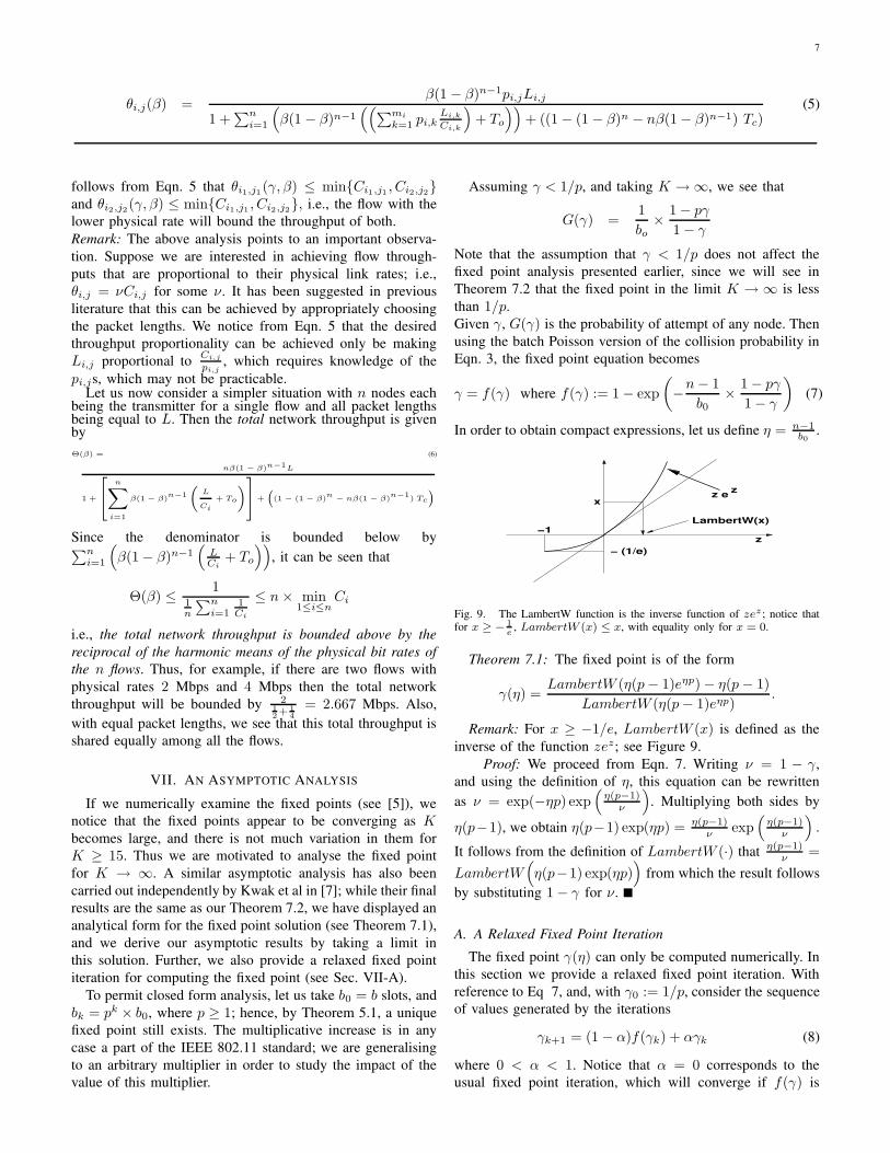
Theorem 7.1: The fixed point is of the form

γ(η) =LambertW (η(p − 1)eηp) − η(p − 1)

LambertW (η(p − 1)eηp).

Remark: For x ≥ −1/e, LambertW (x) is defined as theinverse of the function zez; see Figure 9.

Proof: We proceed from Eqn. 7. Writing ν = 1 − γ,and using the definition of η, this equation can be rewrittenas ν = exp(−ηp) exp

(

η(p−1)ν

)

. Multiplying both sides by

η(p−1), we obtain η(p−1) exp(ηp) = η(p−1)ν

exp(

η(p−1)ν

)

.

It follows from the definition of LambertW (·) that η(p−1)ν

=

LambertW(

η(p−1) exp(ηp))

from which the result followsby substituting 1 − γ for ν.

A. A Relaxed Fixed Point Iteration

The fixed point γ(η) can only be computed numerically. Inthis section we provide a relaxed fixed point iteration. Withreference to Eq 7, and, with γ0 := 1/p, consider the sequenceof values generated by the iterations

γk+1 = (1 − α)f(γk) + αγk (8)

where 0 < α < 1. Notice that α = 0 corresponds to theusual fixed point iteration, which will converge if f(γ) is

8

a contraction. The above iteration is called a relaxed fixedpoint iteration. We will now provide a condition on α thatwill ensure that the iterates converge to the fixed point.

First of all, since f(γ) is continuous, it is clear from theiteration in Eqn. 8 that if the sequence of iterates converge thenthey must converge to the fixed point. It is also clear that if, foreach k, γk ≥ f(γk) then the sequence {γk} is nonincreasing.This follows because γk+1 = (1−α)f(γk)+αγk ≤ γk if andonly if f(γk) ≤ γk. Thus, since γk ≥ 0, for the convergenceof the sequence {γk} it suffices to ensure that γk ≥ f(γk) forall k.

Now, it can easily be shown that the derivative of f(γ) atγ = 1/p is given by D := −n−1

b0

p2

p−1 , and that, for γk+1 ≤ γk

f(γk+1) − f(γk) ≤ |D| (γk − γk+1)

From this inequality we can see that to ensure f(γk) ≤ γk,for all k, it is sufficient to ensure that, for all k, |D| (γk −γk+1) ≤ γk+1 − f(γk). Using the iteration in Eqn. 8 this isequivalent to ensuring that, for all k, |D|(1−α)(γk−f(γk)) ≤α(γk − f(γk)). Hence it suffices that |D|(1−α) ≤ α, or thatα ≥ |D|/(|D| + 1). Thus, for example, with n = 10 nodes,b0 = 16 slots, and p = 2, the relaxed fixed point iteration withα such that 2.25

3.25 < α < 1 will yield the unique fixed pointγ(η).

B. Taking n to ∞

We now wish to take n to ∞ and study the limit of the fixedpoint solution obtained in Theorem 7.1. For this we need thefollowing properties of the LambertW function.

Lemma 7.1:1) For a > 0,

limx→∞

LambertW (axex)

x= 1 (9)

2) For a > 0

limx→∞

(LambertW (axex) − x) = ln a

3) For 0 < a ≤ 1, LambertW (axex) ≤ x4) For 0 < a < 1, the convergence in Eqn. 9 is from below.

Proof: Provided in the Appendix.The following result is now obtained by applying

Lemma 7.1 to the expression for γ in Theorem 7.1.Theorem 7.2:

1) γ(η) < 1/p,2) limn→∞ γ(η) ↑ 1/p,3) limn→∞ nβ ↑ ln( p

p−1 ).The following result provides the rate of convergence in

Theorem 7.2.Theorem 7.3: We have:

limn→∞

ηp

(

γ(η) −1

p

)

= a ln(a) where a =p − 1

p.

Proof: Define x = ηp. From Theorem 7.1 we have:

γ(η) −1

p= 1 −

x

LambertW (axex)a −

1

p

= a

(

1 −x

LambertW (axex)

)

Thus we obtain:

ηp

(

γ(η) −1

p

)

= ax

LambertW (axex)(LambertW (axe

x) − x)

Now using Parts 1 and 2 of Lemma 7.1, we obtain the desiredconclusion.

Remarks 7.1:1) Theorem 7.2 provides explicit expressions for the collisionprobability and the fixed point for large K and a large numberof nodes. We see that for large n the collision probabilityis directly related to the back-off multiplier p, and is thereciprocal of this multiplier.2) We also see that nβ, the mean attempt rate per slot, goes toln( p

p−1 ), and hence the attempt probability per node (duringback-off periods) behaves like O( 1

n). This lends some support

to the original assumption that from the point of view of anode the attempt process of the other nodes can be viewedas an independent process with i.i.d. batch Poisson arrivals insuccessive slots.

C. Asymptotic Aggregate ThroughputLet us now consider n nodes handling n flows with all the

flows having the same transmission rate, C. The aggregatethroughput of the network is given by (compare with Eqn. 6)

Θ(β) =nβe−nβL

1 +(

nβe−nβ(

LC

+ To

))

+ ((1 − e−nβ− nβe−nβ) Tc)

We infer from this equation that, as n → ∞ the aggregatethroughput converges to

τ (p) :=(1 −

1p)L

1ln(

pp−1

)+ (1 −

1p)( L

C+ To) +

( 1p

ln(p

p−1)− (1 −

1p))

Tc

The following result is then immediately obtainedTheorem 7.4:

1) limp→∞ τ(p) = 0,2) limp→1 τ(p) = 0,3) τ(p) is maximised at

p =Tc

Tc+1

LambertW(

− 1e· Tc

(Tc+1)

)

+ Tc

Tc+1

Remarks 7.2: 1) The behaviour of the aggregate throughputas p goes to its two extremes is as expected. If p → 1 thenthe nodes do not increase their back-off intervals in responseto collisions. The collision probability becomes large and thethroughput drops to 0. Obviously, as p → ∞ collisions causea drastic reduction in attempts essentially shutting the nodesoff.

2) In an attempt to see what the above asymptotic resultshave to say about realistic network parameters, in Figure 10we plot the aggregate throughput for finite K and finite n,using the formula in Eqn. 6 with equal transmission rate forall the flows. We see that the throughput increases steeply for1 < p < 2, but is quite flat with p after p = 2. There isan optimal value of p, but unless p is very close to 1, thethroughput is not very sensitive to p. It can be seen that the

9

0 1 2 3 4 5 6 7 8 9 100

1

2

3

4

5

6

7

8

9

10

back−off multiplier, p

aggre

gate

throu

ghpu

t (Mbp

s)

n=10

n=60

Fig. 10. Aggregate throughput plotted vs. the back-off multiplier p for twovalues values of n. The network parameters are K = 10, b0 = 16 slots,data packet length 8000 bits, packet overhead 592 bits, slot time 20 µs,transmission rate for all flows 11 Mbps, fixed (rate independent) data packettransmission overhead 52 slots, collision overhead 17 slots.

back-off multiplier used in the standard, i.e., p = 2, is adequateunless the number of nodes becomes very large. For Tc = 17(slots), the third part of Theorem 7.4 returns p = 3.85, whichcompares well with the curve for n = 60 in Figure 10.

VIII. APPLICATION TO THE ANALYSIS OF TCPCONTROLLED FILE TRANSFERS

A. Some Modeling Assumptions

We will make the following assumptions:A1: The files are infinitely long. Thus we do not deal

with web transfers. Practically, this assumption means thatour analysis applies to large file transfers, such as software,document, or media downloads.

A2: The modulation scheme and bit rate of the physicalconnection between a pair of communicating wireless devicesis ideally adapted (but fixed) so that there is no packet lossowing to bit errors. Further, the retransmission time-out at eachTCP transmitter is large enough so that time-outs never takesplace.

A3: At the transmitter of each wireless device the capacityof the buffer is such that there is no packet loss. Thisassumption effectively holds in practice if the number of filetransfer connections through a node is small enough so thatthe sum of the maximum TCP windows of all the connectionsis less than the buffer size. For, say, 10 connections, this wouldtypically require a buffer of no more than 512 KB.

A4: The file transfer throughputs are bottlenecked onlyby the rates they obtain over the WLAN. For example, thetransfers could be between the wireless devices across anad hoc WLAN, or, in the infrastructure case, between thewireless devices and devices attached to a high speed wiredLAN to which the AP is attached. For transfers within abuilding or campus this assumption is practically valid sincemost wired LANs are based on 100 Mbps to 1 Gbps Ethernet.

Owing to Assumption A1 it makes sense to talk aboutthe long run time average throughput of a transfer. FromAssumptions A2 and A3 it follows that the TCP windowof each connection grows to its maximum value, and byAssumption A4, each data packet or ACK of all the TCP

connections will be queued at the transmitter of one of theWLAN devices.

Let us adopt the following connection model. There arem connections, indexed by j, 1 ≤ j ≤ m. The source nodeof connection j is denoted by s(j), and the receiver node isdenoted by r(j)( 6= s(j)). Thus, for connection j, the TCPACKs will queue up at the transmitter of node r(j). The datapacket length for connection j is denoted by Lj and the ACKpacket length by L

(ack)j . In general, each node will transmit

data packets for some connections and ACK packets for otherconnections.

In order to use the “saturated queues” analysis presentedearlier in the paper, we make the following additional assump-tion

A5: The configuration of the TCP connections and the sizesof their windows are such that the transmitter queues of thewireless devices never empty out.Remark: This assumption is made to permit us to use thefixed point analysis presented earlier in the paper. It, however,considerably restricts the scenarios to which the analysis willapply. For example, the common situation of two or moredevices simultaneously downloading files via an AP is notcovered by our analysis. This is because the AP needs to sendmany more packets for each packet that each of the devicessends, and hence the device queues will empty out, violatingour saturated queues assumption.

We will utilise Assumption A5 as follows. Recall ourdiscussion in Sec. VI. If all the n queues always have packetsto send, then they always contend for the channel, and eachsuccessful attempt “belongs” to each of the queues with equalprobability, 1/n.

B. A Formula for Connection Throughput

Let us now focus only on the successful attempt instants.Such a success belongs to node i with probability 1

n. The

HOL packet at that node is then transmitted. If this packet isof length L and the transmission rate is C then a time L

C+To

elapses. If the packet transmitted is a data packet then possiblyan ACK is inserted into the transmitter queue of the receivingnode (note that if delayed ACKs are used then not every datapacket causes an ACK to be generated). On the other hand,if the packet transmitted is an ACK packet then one or morepackets are inserted into the transmitter queue of the receivingnode. Thus the queues can be viewed as evolving only atsuccessful polling instants. This is an important observationas it allows us to ignore the back-off periods while analysingthe evolution of the packet queues. Note that this observationdoes not hold if there are finite rate open-loop arrival processesinto the nodes, as these arrival processes will cause the queuesto evolve even during back-off periods.

From the above observations, we can now proceed byanalysing the discrete time random polling model shown inFigure 11. The discrete “time” in this model evolves overpackets. Note that we do not need to be concerned with packetlengths (data or ACK), or physical bit rates. We will see thatall we need from this model is the fraction of polls to a queuethat find packets of each type at the head-of-the-line. There

10

θj(β) =

β(1 − β)n−1hs(j),jLj

1 +∑n

i=1β(1 − β)n−1

((

∑

{j:s(j)=i}hi,j

Lj

Ci,r(j)+

∑

{j:r(j)=i}h

(ack)i,j

L(ack)j

Ci,s(j)

)

+ To

)

+ (1 − (1 − β)n− nβ(1 − β)n−1) Tc

(10)

random orderof visit, withprobability 1/n

. . .

. .

1

2

TCP connection from node n to node 2

TCP connection from node 2 to node 1

n

Fig. 11. There are several TCP connections, modeled as “chains” ofcustomers with a fixed population (the window size) circulating in a randompolling network. The solid arrows between the queues show the direction ofTCP data transfer for a connection, and the dashed arrows show the directionof TCP ACK transmission. The n transmitters are served in random orderwith equal probability for each node.

are several TCP connections modeled as “chains” or classes ofcustomers circulating between pairs of nodes. The populationsof the chains are the TCP window sizes. If the delayed ACKparameter for a connection is greater than 1 (let us say 2),then at the receiving node for that connection 2 data packetsgive rise to one ACK packet. We can view this ACK packetas being a batch of 2, that is served together.

The state of the random polling model is the position andtype of each packet in each queue. This process evolves overpacket times. It is easy to see that the evolution of this rathercomplicated process is Markovian. Analysis of this Markovchain will yield the following probabilities, that will be usedin the throughput formulas.

hi,j : the probability that at a polling instant the HOLpacket at node i is a data packet from connectionj

h(ack)i,j :the probability that at a polling instant the HOL

packet at node i is an ACK packet for connection j(for which node i is the receiver node, i.e., i = r(j))

By the observations made just before these definitions, wecan conclude that the probabilities hi,j and h

(ack)i,j do not

depend on data and ACK packet lengths, nor on the physicalbit rates of the connections. These probabilities will dependonly on the maximum TCP window sizes, the delayed ACKthresholds, and the connection configurations (i.e., whichnodes carry which connections). We also note that once wehave these probabilities, the throughput of connection j can beimmediately obtained as in Eqn. 10 (see also Eqn. 5), where(γ, β) are obtained from the fixed-point analysis. This formulahas the same form as the one in Eqn. 5. In the numeratorthe term β(1 − β)n−1 is the probability that node s(j) has asuccess, hs(j),j is the probability that the HOL packet belongs

to connection j, and when both these events occur connectionj has a “reward” of Lj bits. The denominator is the meanlength of a back-off and attempt cycle.

Remarks 8.1:1) To be technically correct Eqn. 10 should have been obtainedas the ratio of two expectations with respect to the stationarydistribution of the Markov chain describing the random pollingmodel. We have shown only the final result in terms of theHOL probabilities at the polling instants, as this is simple andintuitively clear.

2) In Eqn. 5 the HOL probabilities were obtained from theratios of the open-loop arrival rates into the queues. In Eqn. 10,however, the HOL probabilities will need to be obtained fromthe packet level analysis of the random polling model shownin Figure 11. We will show how this is done in the nextsubsection.

3) The denominator of the expression now includes a termfor the service provided to TCP ACKs.

4) We have used the fact that all data packets within TCPconnection j have the same length Lj , and the ACK packetswithin TCP connection j have the same size L

(ack)j . If this

were not the case then we would need to make a moreelaborate definition of the HOL probabilities which wouldhave to include the probability of finding packets of eachpossible length.

C. Obtaining the HOL Probabilities

Let λj be the throughput of connection j through its sendernode s(j) in the random polling model shown in Figure 11.Thus λj the average number of packets of connection j thatpass through the node s(j) per packet served in the pollingmodel.

Theorem 8.1: If at each success instant one of the nodesis polled with equal probability (i.e., we have the model inFigure 11) then hs(j),j = λjn.

Proof: Let πs(j),j denote the fraction of packet servicesin the model of Figure 11 during which the HOL positionat node s(j) is occupied by a data packet of connection j.Since the mean time that a packet spends in the HOL positionis n, by Little’s Theorem we have πs(j),j = λjn. Owing torandom polling, the HOL position at node s(j) is observed bya Bernoulli process with probability of “success” equal to 1

n.

Hence by the result that Bernoulli “arrivals” see time averages,we can conclude that hs(j),j = πs(j),j = λjn.

Remarks 8.2: 1) If the throughput of ACKs for connectionj through its receiver node r(j) is λ

(ack)j then by the same

argument as in Theorem 8.1 it follows that h(ack)s(j),j = λ

(ack)j n.

11

0 10 20 30 40 50 602.05

2.1

2.15

2.2

2.25

2.3

2.35

2.4

2.45

2.5x 106

Number of connections

Aggre

gated

throu

ghpu

t (b/s)

FPAns2

Fig. 12. Plot of aggregate TCP controlled file transfer throughput vs. numberof simultaneous transfers over an IEEE 802.11b network. Results obtainedfrom the approximate analysis, and from ns2 simulations are shown, with95% confidence intervals. In the simulation the IEEE 802.11 parameters areused, with data rate: 11 Mbps, control rate: 2 Mbps.

2) We note that the hypothesis of the Theorem 8.1 that “ateach success instant one of the nodes is polled with equalprobability” requires the saturation assumption, i.e., Assump-tion A5, to hold. There are TCP connection configurations forwhich this assumption will not hold. For example considera single TCP connection from Node 1 to Node 2. The TCPreceiver uses a delayed ACK threshold of 2; i.e., it returnsone ACK for two received data packets. Clearly over a largenumber of packet transmitted we cannot say that about halfwill come from Node 1 and the other half from Node 2. In thiscase the receiver node will tend to empty out and the saturationassumption will not apply. On the other hand if Node 2 wasalso sending to Node 1 then our analysis will apply.

3) In view of Theorem 8.1 we need to analyse the randompolling model and obtain the λjs and the λ

(ack)j s, and this will

yield the HOL probabilities needed in the throughput formula.

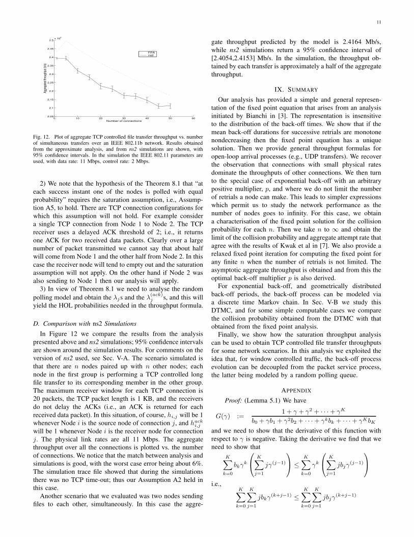
D. Comparison with ns2 Simulations

In Figure 12 we compare the results from the analysispresented above and ns2 simulations; 95% confidence intervalsare shown around the simulation results. For comments on theversion of ns2 used, see Sec. V-A. The scenario simulated isthat there are n nodes paired up with n other nodes; eachnode in the first group is performing a TCP controlled longfile transfer to its corresponding member in the other group.The maximum receiver window for each TCP connection is20 packets, the TCP packet length is 1 KB, and the receiversdo not delay the ACKs (i.e., an ACK is returned for eachreceived data packet). In this situation, of course, hi,j will be 1whenever Node i is the source node of connection j, and hack

i,j

will be 1 whenever Node i is the receiver node for connectionj. The physical link rates are all 11 Mbps. The aggregatethroughput over all the connections is plotted vs. the numberof connections. We notice that the match between analysis andsimulations is good, with the worst case error being about 6%.The simulation trace file showed that during the simulationsthere was no TCP time-out; thus our Assumption A2 held inthis case.

Another scenario that we evaluated was two nodes sendingfiles to each other, simultaneously. In this case the aggre-

gate throughput predicted by the model is 2.4164 Mb/s,while ns2 simulations return a 95% confidence interval of[2.4054,2.4153] Mb/s. In the simulation, the throughput ob-tained by each transfer is approximately a half of the aggregatethroughput.

IX. SUMMARY

Our analysis has provided a simple and general represen-tation of the fixed point equation that arises from an analysisinitiated by Bianchi in [3]. The representation is insensitiveto the distribution of the back-off times. We show that if themean back-off durations for successive retrials are monotonenondecreasing then the fixed point equation has a uniquesolution. Then we provide general throughput formulas foropen-loop arrival processes (e.g., UDP transfers). We recoverthe observation that connections with small physical ratesdominate the throughputs of other connections. We then turnto the special case of exponential back-off with an arbitrarypositive multiplier, p, and where we do not limit the numberof retrials a node can make. This leads to simpler expressionswhich permit us to study the network performance as thenumber of nodes goes to infinity. For this case, we obtaina characterisation of the fixed point solution for the collisionprobability for each n. Then we take n to ∞ and obtain thelimit of the collision probability and aggregate attempt rate thatagree with the results of Kwak et al in [7]. We also provide arelaxed fixed point iteration for computing the fixed point forany finite n when the number of retrials is not limited. Theasymptotic aggregate throughput is obtained and from this theoptimal back-off multiplier p is also derived.

For exponential back-off, and geometrically distributedback-off periods, the back-off process can be modeled viaa discrete time Markov chain. In Sec. V-B we study thisDTMC, and for some simple computable cases we comparethe collision probability obtained from the DTMC with thatobtained from the fixed point analysis.

Finally, we show how the saturation throughput analysiscan be used to obtain TCP controlled file transfer throughputsfor some network scenarios. In this analysis we exploited theidea that, for window controlled traffic, the back-off processevolution can be decoupled from the packet service process,the latter being modeled by a random polling queue.

APPENDIX

Proof: (Lemma 5.1) We have

G(γ) :=1 + γ + γ2 + · · · + γK

b0 + γb1 + γ2b2 + · · · + γkbk + · · · + γKbK

and we need to show that the derivative of this function withrespect to γ is negative. Taking the derivative we find that weneed to show that

K∑

k=0

bkγk

K∑

j=1

jγ(j−1)

≤

K∑

k=0

γk

K∑

j=1

jbjγ(j−1)

i.e.,K

∑

k=0

K∑

j=1

jbkγ(k+j−1) ≤

K∑

k=0

K∑

j=1

jbjγ(k+j−1)

12

or, equivalently, we need to show that

2K∑

n=1

γ(n−1)

min{n,K}∑

j=max{(n−K),1}

k=(n−j)

j(bj − bk) ≥ 0

Now we consider each term∑min{n,K}

j=max{(n−K),1}

k=(n−j)

j(bj − bk) and

show that it is nonnegative. To this end, define

m(n) = |{(j, k) : j + k = n, 1 ≤ j ≤ K, 0 ≤ k ≤ K}|,

where | · | denotes set cardinality. When k = j, jbj − jbk = 0and the corresponding term vanishes from the sum. Also, kequals 0 only when j = n and 1 ≤ n ≤ K. Hence, simplifyingthe above expression, we get,

max{(n−K),1}+bm2 c−1

∑

j=max{(n−K),1}

(

((n − j) − j)(bn−j − bj) +

n(bn − b0)1{1≤n≤K}

)

which is nonnegative since, in the range of the sum, (n −j) − j ≥ 0 and bn−j − bj ≥ 0. It is also easily seen that thederivative of G(·) is strictly negative for γ > 0 if the bk arenot all equal, this implies that G(·) is strictly decreasing inthis case.

Proof: (Theorem 7.1) This is just a simple manipulationof the fixed point equation to get it into the form of theLambertW function. The fixed point equation is

γ = 1 − e

(

−(n−1)× 1b0

× 1−pγ

1−γ

)

which can be rewritten as (1 − γ) = e−ηpeη(p−1)(1−γ) . This

expression can be rearranged as follows

η(p − 1) eηp =η(p − 1)

(1 − γ)e

η(p−1)

(1−γ)

It follows, from the definition of the LambertW function (andutilising the fact that p > 1) that

η(p − 1)

(1 − γ)= LambertW (η(p − 1) eηp)

The result follows by rearranging the equation to extract γ.Proof: (Lemma 7.1)

1) For x ≥ 0, write z(x) = LambertW (axex), i.e.,z(x)ez(x) = axex. It is easily seen that for x > 0,z(x) > 0, and z(x) ↑ ∞ for x → ∞. Now, takingnatural logarithms, we obtain, for all x > 0, ln z(x) +z(x) = ln ax + x, or

z(x)

x=

ln axx

+ 1ln z(x)z(x) + 1

which, on taking x → ∞ yields the desired result sinceln ax

xand ln z(x)

z(x) both go to 0.2) Again, writing z(x) = LambertW (axex), and using

the relation ln z(x) + z(x) = ln ax + x, we have

z(x) − x = ln(ax) − ln z(x) = ln

(

ax

z(x)

)

Since limx→∞(x/z(x)) = 1, by Part 1 of this lemma,we obtain the desired conclusion.

3) By definition, LambertW (xex) = x, and LambertW ismonotone increasing for positive arguments. Hence, for0 < a ≤ 1, LambertW (axex) ≤ x.

4) Follows by combining the previous two parts.Proof: (Theorem 7.2) Observe that we can write

LambertW (η(p − 1)eηp) asLambertW ( p−1

pηpeηp), with p−1

pbeing less than 1, by virtue

of p > 1. The first two parts now follow upon usingLemma 7.1 in

γ(η) =LambertW (η(p − 1)eηp) − η(p − 1)

LambertW (η(p − 1)eηp)

The limit for nβ is obtained as follows. We have

(1 − γ) = e−(n−1)β

Rearranging we have

(n − 1)β = − ln(1 − γ)

It follows that

nβ =n

n − 1(n − 1)β ↑n→∞ ln(

p

p − 1)

ACKNOWLEDGEMENTS

We are grateful to Chadi Barakat for some useful discus-sions.

REFERENCES

[1] F. Baccelli and S. Foss. On the saturation rule for the stability of queues.J. Appl. Prob., 32(2):494–507, 1995.

[2] G. Berger-Sabbatel, F. Rousseau, M. Heusse, and A. Duda. Performanceanomaly of 802.11b. In Proceedings of IEEE Infocom 2003. IEEE, 2003.

[3] G. Bianchi. Performance analysis of the IEEE 802.11 distributed coor-dination function. IEEE Journal on Selected Areas in Communications,18(3):535–547, March 2000.

[4] F. Cali, M. Conti, and E. Gregori. IEEE 802.11 protocol: Design andperformance evaluation of an adaptive backoff mechanism. IEEE Journalon Selected Areas in Communications, 18(9):1774–1780, September2000.

[5] Anurag Kumar, Eitan Altman, Daniele Miorandi, and Munish Goyal. Newinsights from a fixed point analysis of single cell IEEE 802.11 wirelessLANs. In Proceedings IEEE Infocom, 2005. Also Technical Report No.RR-5218, INRIA, Sophia-Antipolis, France, June 2004.

[6] Anurag Kumar and Deepak Patil. Stability and throughput analysis ofunslotted CDMA-ALOHA with finite numer of users and code sharing.Telecommunication Systems, 8:257–275, 1997.

[7] B.-J. Kwak, N.-O. Song, and L. E. Miller. Analysis of the stability andperformance of exponential backoff. In Proceedings of IEEE WCNC,2003.

[8] Stefan Mangold, Sunghyun Choi, Peter May, Ole Klein, Guido Hiertz,and Lothar Stibor. IEEE 802.11e wireless LAN for quality of service. InProc. European Wireless (EW 2002), February 2002.

[9] Venkatesh Ramaiyan, Anurag Kumar, and Eitan Altman. Fixed pointanalysis of single cell IEEE 802.11e WLANs : Uniqueness, multistabilityand throughput differentiation. In ACM Sigmetrics, June 2005.

13

Anurag Kumar obtained his B.Tech. degree inElectrical Engineering from the Indian Institute ofTechnology at Kanpur. He obtained the PhD degreefrom Cornell University. He was then with BellLaboratories, Holmdel, N.J., for over 6 years. Since1988 he has been with the Indian Institute of Science(IISc), Bangalore, in the Dept. of Electrical Commu-nication Engineering, where he is now a Professor,and is also the Chairman of the department. From1988 to 2003 he was the Coordinator at IISc of theEducation and Research Network Project (ERNET),

India’s first wide-area packet switching network. His area of research isCommunication Networking; specifically, modeling, analysis, control andoptimisation problems arising in communication networks and distributedsystems. He has been elected Fellow of the IEEE, and the Indian NationalScience Academy (INSA), both from 2006, and has been a Fellow of theIndian National Academy of Engineering (INAE) since 1998. He has receivedIETE’s (Institution of Electronics and Telecommunications Engineers) CDILBest Paper Award (1993), and IETE’s S.V.C. Aiya Award for Telecom Edu-cation (2001). He is an associate editor of IEEE Transactions on Networking,and an area editor of IEEE Communications Surveys and Tutorials. Heis a coauthor of the advanced text-book “Communication Networking: AnAnalytical Approach,” by Kumar, Majunath and Kuri, published by Morgan-Kaufman/Elsevier.

Eitan Altman received the B.Sc. degree in electri-cal engineering (1984), the B.A. degree in physics(1984) and the Ph.D. degree in electrical engineer-ing (1990), all from the Technion-Israel Institute,Haifa. In (1990) he further received his B.Mus.degree in music composition in Tel-Aviv univer-sity. Since 1990, he has been with INRIA (Na-tional research institute in informatics and control)in Sophia-Antipolis, France. His current researchinterests include performance evaluation and controlof telecommunication networks and in particular

congestion control, wireless communications and networking games. Heis in the editorial board of several scientific journals: Stochastic Mod-els, JEDC, COMNET, SIAM SICON and WINET. He has been the gen-eral chairman and the (co)chairman of the program committee of sev-eral international conferences and workshops (on game theory, network-ing games and mobile networks). More informaion can be found athttp://www.inria.fr/mistral/personnel/Eitan.Altman/me.html

Daniele Miorandi received his ”Laurea” (summacum laude) and Ph.D. degrees from Univ. of Padova(Italy) in 2001 and 2005, respectively. He cur-rently holds a researcher position at CREATE-NET,Trento (Italy). In 2003/04 he spent 12 months ofhis doctoral thesis visiting the MAESTRO teamat INRIA Sophia Antipolis (France). His researchinterests include design and analysis of bio-inspiredcommunication paradigms for pervasive computingenvironments, analysis of TCP performance overwireless/satellite networks, scaling laws for large-

scale information systems, protocols and architectures for wireless meshnetworks.

Munish Goyal obtained his Masters and PhD de-grees in Telecommunications from the Indian In-stitute of Science, Bangalore, India and a Bache-lors degree in Electronics and Communication fromthe Indian Institute of Technology, Roorkee, India.Currently, he is a postdoctoral research fellow atthe ARC Center of Excellence for Mathematicsand Statistics of Complex Systems, University ofMelbourne, Australia. His research interests includemodelling, analysis and control problems arisingin stochastic systems especially telecommunication

systems.