new models and algorithms for multidimensional approximate

New Models and Algorithms forMultidimensional ApproximatePattern Matching

RICARDO BAEZA-YATES1, Dept. of Computer Science, Universityof Chile. Blanco Encalada 2120, Santiago, [email protected]

GONZALO NAVARRO1, Dept. of Computer Science, University ofChile. Blanco Encalada 2120, Santiago, [email protected]

ABSTRACT:We focus on how to compute the edit distance (or similarity) between two imagesand the problem of approximate string matching in two dimensions, that is, to find a pattern ofsizem�m in a text of sizen� n with at mostk errors (character substitutions, insertions anddeletions). Pattern and text are matrices over an alphabet of size�. We present new models andgive the first sublinear time search algorithms for the new and the existing models.

The only existing model just considers errors along one dimension. The associated approx-imate search algorithms use dynamic programming and are relatively expensive (O(m2n2) orO(k2n2)). For this model we present a filtering algorithm which avoids verifying most of thetext with dynamic programming. This filter is based on one-dimensional multipattern approxi-mate searching. The average complexity of our resulting algorithm isO(n2k log�m =m2) fork < m(m+ 1)=(5 log�m), which is optimal and matches the best previous result that allowsonly substitutions. We present other slower filtration algorithms that however work for highererror levels.

We then consider more general models to compare images. We present new similarity mea-sures and the algorithms to compute them. We then focus on oneof the models, which allowsthe errors to occur along any dimension, and extend it to the general case where pattern and textared-dimensional. This edit distance can be computed inO(d!m2d) time andO(d!m2d�1)space. We also present the first sublinear-time (on average)searching algorithm (i.e. not all textcells are inspected), which isO(knd=md�1) time fork < (m=(d(log�(m=d))))d�1.

Keywords: Pattern matching in images, edit distance, Levenshtein distance

1 Introduction

Approximate pattern matching is the problem of finding a pattern in a text allow-ing errors (insertions, deletions, substitutions) of characters. A number of importantproblems related to string processing lead to algorithms for approximate string match-ing: text searching, pattern recognition, computational biology, audio processing, etc.

1This work has been supported in part by Fondecyt grant 1-990627.

J. of Discrete Algorithms, Vol. 0 No. 0, pp. 1–29, 0000 c Hermes Science Publications

2 J. of Discrete Algorithms, Vol. 0 No. 0, 0000

Approximate two dimensional pattern matching has applications, for instance, in com-puter vision (i.e. searching a subimage inside a large image) and OCR. In three di-mensions, the problem has applications in some types of medical data (e.g. MRI brainscans) and in biocomputing (e.g. detecting protein patterns on the surface of threedimensional virus reconstructions).

For one dimension this problem is well-known, and is modeledusing the edit dis-tance. Theedit distancebetween two stringsA andB, ed(A;B), is defined as theminimum number ofedit operationsthat must be carried out to make them equal. Theallowed operations are insertion, deletion and substitution of characters inA or B.The problem ofapproximate string matchingis defined as follows: given a textT oflengthn, and a patternP of lengthm, both being sequences over an alphabet� ofsize�, find all segments (or “occurrences”) inT whose edit distance toP is at mostk, where0 < k < m. The classical solution isO(mn) time and involves dynamicprogramming [32].

Krithivasan and Sitalakshmi (KS) [24] proposed a simple extension to two dimen-sions. Given two images of the same size, the edit distance isthe sum of the editdistance of the corresponding row images. This definition isjustified when the imagesare transmitted row by row and there are not too many communication errors (e.g.photocopy images, where most errors come from the mechanical traction mechanismalong one dimension only, or images transmitted by fax), butit is not appropriate oth-erwise. Using this model they define an approximate search problem where a subim-age of sizem �m is searched into a large image of sizen � n, which they solve inO(m2n2) time using a generalization of the classical one-dimensional algorithm.

Using this model we improve the expected case using a filter algorithm based onmultiple one-dimensional approximate string matching, inthe same vein of [14, 13,12]. Our algorithm hasO(n2k log�m =m2) average-case behavior fork < m(m +1)=(5 log�m), usingO(m2) space. This time matches the best known result for thesame problem allowing only substitutions and is optimal [22], being the restriction onk only a bit more strict. For higher error levels, we present analgorithm with timecomplexityO(n2k=(wp�)) (wherew is the size in bits of the computer word), whichworks fork < m(m + 1)(1 � e=p�). We also show that this limit onk cannot beimproved.

However, for many other problems, the KS distance does not reflect well simplecases of approximate matching in different settings. For example, we could have amatch that only has the middle row of the pattern missing. In the definition above, theedit distance would beO(m2) if all pattern rows are different. Intuitively, the rightanswer should be at most2m, because onlym characters were deleted in the patternandm characters are inserted at the bottom.

In this paper we extend the edit distance to two dimensions lifting the problemjust mentioned and also extending the edit distance to images of different shapes.We define different distances and give algorithms to computethem, as well as theassociated approximate search algorithms.

Among the more general extensions that we define, we focus in the RC model,where the errors can occur along rows or columns at any time. This model is muchmore robust and useful for more applications. We extend the model tod dimensions

New Models and Algorithms for Multidimensional Approximate Pattern Matching 3

and present an edit distance algorithm with time complexityO(d!m2d). We also give anew filtering algorithm that allows quickly discarding large parts of the text that cannotcontain a match. This algorithm searches the pattern in average timeO(knd=md�1)for k < (m=(d(log�(m=d))))d�1. After that error level the filter changes its cost butremains better than dynamic programming fork � md�1=(d(log�(m=d)))(d�1)=d.

This paper is organized as follows. First we discuss the basic concepts and previouswork on pattern matching with errors and image similarity. Next, we consider thebasic KS model and give new filters to speed up the search. In Section 4 we introducenew notions of similarity between two-dimensional images,together with algorithmsto compute the edit distance. Section 5 presents how to search a pattern in a text underthe new model. Then we extend one of the models to more dimensions and give fastfiltering algorithms for approximate searching under that model. Finally, we give ourconclusions. This work is an integrated and revised versionof [7, 9, 28].

2 Basics and Previous Work

We give in this section some basic concepts and review the previous work in the area.We define some terminology first. Given a one dimensional stringS we useSi to de-note itsi-th character, the first one corresponding toi = 1. Si::j denotes the substringstarting at characteri and ending at characterj, both inclusive. A character of a two-dimensional stringS is addressed asSi;j , meaning the character at rowi and columnj. Similarly, rows and columns can be extracted asSi;j1::j2 andSi1::i2;j , respectively,and even sub-matrices such asSi1::i2;j1::j2 .

2.1 One Dimensional Approximate String Matching

The classical dynamic programming algorithm [29] to compute the edit distance be-tween two one-dimensional stringsA andB of lengthm andn computes a matrixC0::m;0::n. The valueCi;j holds the edit distance betweenA1::i andB1::j . The con-struction algorithm is as followsCi;0 i ; C0;j jCi;j if Ai = Bj then Ci�1;j�1 else 1 +min(Ci�1;j�1; Ci�1;j ; Ci;j�1)and the distanceed(A;B) is the final value ofCm;n. The rationale of the formula isthat if Ai = Bj then the cost to convertA1::i into B1::j is that of convertingA1::i�1into B1::j�1. Otherwise we have to make one error and select among three choices:(a) convertA1::i�1 intoB1::j�1 and replaceAi byBj , (b) convertA1::i�1 intoB1::jand deleteAi, and( ) convertA1::i intoB1::j�1 and insertBj .

This algorithm takesO(mn) space and time. It is easily adapted to search a patternP in a textT allowing up tok errors [32]. In this case we want to report all the textpositionsj such that a suffix ofT1::j matchesP with at mostk errors. This time theconstruction formula isCi;0 i ; C0;j 0Ci;j if Pi = Tj then Ci�1;j�1 else 1 +min(Ci�1;j�1; Ci�1;j ; Ci;j�1)


where the only change is that a pattern of length zero matcheswith no errors at anytext position. All the positionsj such thatCm;j � k are reported. This takesO(mn)time. The space can be reduced toO(m) by noticing that only the old and new columnof the matrix need to be stored.

This solution was later improved by a number of algorithms [27]. One of specialinterest to this work is a filtering algorithm [34, 11, 10]. Afilter is a fast algorithmthat can discard most of the text by checking a necessary condition. All filters have amaximum error level up to where they are useful. This filter cutsP in k + 1 pieces.Any occurrence with up tok errors must contain one of those pieces unchanged. Thisis obvious sincek errors cannot alter thek + 1 pieces given that the edit operationsthat we consider cannot alter two pieces at the same time. Thealgorithm simply scansthe text using a multipattern exact search algorithm for allthe pieces. Each time apiece is found, it uses dynamic programming over an area of lengthm+2k where theapproximate occurrence can be found.

The multipattern search can be carried out inO(n) worst-case search time by usingan Aho-Corasick machine [1], or inO(n=m) best-case time using Commentz-Walter[15] or another Boyer-Moore type algorithm adapted to multipattern search. The totalcost of verifications keeps negligible ifk=m � 1=(3 log� m). We callsublinear timethose algorithms that do not inspect all the text characters.

On the other hand, approximate multipattern search has onlyrecently been consid-ered. In [25], hashing is used to search thousands of patterns in parallel, althoughwith only one error. In [8], extensions of [10] and [11] are presented based on super-imposing automata. In [26], a counting filter is bit-parallelized to keep the state ofmany searches in parallel. Most multipattern algorithms are filters able to check for anecessary condition on many patterns at the same time.

2.2 Two Dimensional Pattern Matching

Two dimensional exact string matching was first considered by Bird and Baker [14,13], who obtainO(n2) worst-case time. Good average results are presented by Zhuand Takaoka in [35]. The first good average case result is due to Baeza-Yates andRegnier [12], who obtainO(n2=m) time on average andO(n2) in the worst case. Thiswas improved by Karkkainen and Ukkonen [22] who achieveO(n2 log�(m)=m2)average case time, which is optimal.

Two-dimensional approximate string matching usually considers only substitutionsfor rectangular patterns, which is much simpler than the general case with insertionsand deletions (because in this case, rows and/or columns of the pattern can matchpieces of the text of different length).

If we consider matching the pattern with at mostk substitutions, one of the best re-sults on the worst case is due to Amir and Landau [5] achievingO((k+log �)n2) timebut usingO(n2) space. A similar algorithm is presented in Crochemore and Rytter[16]. Ranka and Heywood [31], on the other hand, solve the problem inO((k+m)n2)time andO(kn) space. Amir and Landau also present a different algorithm running inO(n2 logn log logn logm) time. On average, the best algorithm is due to Karkkainenand Ukkonen [22], with its analysis and space usage improvedby Park [30]. The ex-


pected time isO(n2k log�(m)=m2) for k � m2=(4 log� m), usingO(m2) space(O(k) space on average). This time result is optimal for the expected case. Theyextend their results tod dimensions achieving timeO(dndk log�(m)=md).2.3 The KS Model

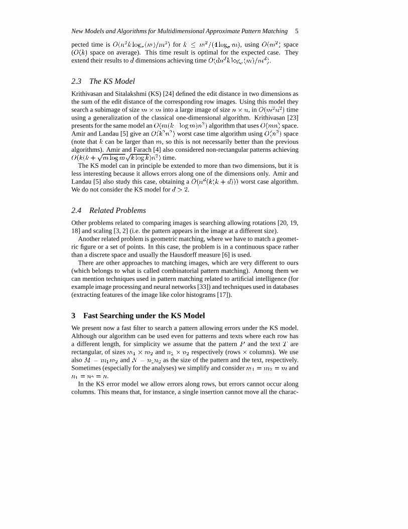
Krithivasan and Sitalakshmi (KS) [24] defined the edit distance in two dimensions asthe sum of the edit distance of the corresponding row images.Using this model theysearch a subimage of sizem�m into a large image of sizen� n, in O(m2n2) timeusing a generalization of the classical one-dimensional algorithm. Krithivasan [23]presents for the same model anO(m(k+logm)n2) algorithm that usesO(mn) space.Amir and Landau [5] give anO(k2n2) worst case time algorithm usingO(n2) space(note thatk can be larger thanm, so this is not necessarily better than the previousalgorithms). Amir and Farach [4] also considered non-rectangular patterns achievingO(k(k +pm logmpk log k)n2) time.

The KS model can in principle be extended to more than two dimensions, but it isless interesting because it allows errors along one of the dimensions only. Amir andLandau [5] also study this case, obtaining aO(nd(k(k + d))) worst case algorithm.We do not consider the KS model ford > 2.

2.4 Related Problems

Other problems related to comparing images is searching allowing rotations [20, 19,18] and scaling [3, 2] (i.e. the pattern appears in the image at a different size).

Another related problem is geometric matching, where we have to match a geomet-ric figure or a set of points. In this case, the problem is in a continuous space ratherthan a discrete space and usually the Hausdorff measure [6] is used.

There are other approaches to matching images, which are very different to ours(which belongs to what is called combinatorial pattern matching). Among them wecan mention techniques used in pattern matching related to artificial intelligence (forexample image processing and neural networks [33]) and techniques used in databases(extracting features of the image like color histograms [17]).

3 Fast Searching under the KS Model

We present now a fast filter to search a pattern allowing errors under the KS model.Although our algorithm can be used even for patterns and texts where each row hasa different length, for simplicity we assume that the pattern P and the textT arerectangular, of sizesm1 �m2 andn1 � n2 respectively (rows� columns). We usealsoM = m1m2 andN = n1n2 as the size of the pattern and the text, respectively.Sometimes (especially for the analyses) we simplify and considerm1 = m2 = m andn1 = n2 = n.

In the KS error model we allow errors along rows, but errors cannot occur alongcolumns. This means that, for instance, a single insertion cannot move all the charac-


ters of its column one position down, or we cannot performm2 deletions along a rowand eliminate the row. All insertions and deletions displace the characters of the rowthey occur in.

In this simple model every row is exactly where it is expectedto be in an exactsearch. That is, we can see the pattern as anm1-tuple of strings of lengthm2, andeach error is a one-dimensional error occurring in exactly one of the strings. Formally,

Definition: Given a patternP (of sizem1 �m2) and a textT (of sizen1 � n2), wesay that the patternP occurs in the text at position(i; j) with at mostk errors ifm1Xr=1 led(Ti+r�1;1::j; Pr;1::m2) � kwhereled(t1::j ; p) = mini21::j ed(ti::j ; p) for one-dimensional stringst andp.

Observe that in this case the problem still makes sense fork > m2, although itmust holdk < m1m2 (since otherwise every text position matches the pattern byperformingm1m2 substitutions).

The natural generalization of the classical dynamic programming algorithm forone dimension to the case of two dimensions was presented in [24]. Its complex-ity is O(MN ), which is also a natural extension of theO(mn) complexity for one-dimensional text. This algorithm usesO(M) extra space, which is the only stateinformation it needs to be started at any text position.

We begin by proving a lemma which allows us to quickly discardlarge areas of thetext.

Lemma: If the pattern occurs withk errors at position(i; j) in the text, andr1; r2; :::rsares different rows in the range1 tom1, thenmint=1::sfled(Ti+rt�1;1::j ; Prt;1::m2)g � bk=s :Proof: Otherwise,led(Ti+rt�1;1::j ; Prt;1::m2) � 1 + bk=s > k=s for all t. Justsumming up the errors in thes selected rows we have strictly more thans� k=s = kerrors and therefore a match is not possible.

The Lemma can be used in many ways. The simplest case is to sets = 1. This tellsus that if we cannot find a rowr of the pattern with at mostk errors at text rowi, thenthe pattern cannot occur at text rowi� r+1. Therefore, we can search forall rows ofthe pattern at text rowm1. If we cannot find a match of any of the pattern rows withat mostk errors, then no possible match begins at text rows1::m1. There cannot bea match at text row 1 because pattern rowm1 was not found at text rowm1. Therecannot be a match at text row 2 because pattern rowm1� 1 was not found at text rowm1. Finally, there cannot be a match at text rowm1 because pattern row 1 was notfound at text rowm1.

This shows that we can search only text rowsi � m1, for i = 1::bn1=m1 . Onlyin the case that we find a match of pattern rowr at text position(i �m1; j), we mustverify a possible match beginning at text rowi � m1 � r + 1. We must perform the


��

��

��

��

��

��

��

��

��

��

��

��

��

3

2 5

n = 24, m = 6, k = 3

pattern row i found

possible position of anapproximate occurrence

text area to verify withdynamic programming

text rows searched with1-dimensional multipattern

i

FIG. 1. Example of how the algorithm works.

verification from text columnj �m2 � k + 1 to j, using the dynamic programmingalgorithm. However, ifk > m2 we can start atj � 2m2 + 1, since otherwise wewould pay more thanm2 insertions, in which case it is cheaper to just performm2substitutions. This verification costsO(m1m22) = O(m3), which is formed bym1applications of the one-dimensional algorithm in a segmentof lengthm2.

To avoid re-verifying the same areas due to overlapping verification requirements,we can force all verifications to be made in ascending row order and ascending columnorder inside rows. By remembering the state of the last verified positions we avoidre-verifying the same columns, this way keeping the worst case of this algorithm atO(m2n2) cost instead ofO(m3n2). Figure 1 shows how the algorithm works.

We have still not explained how to perform a multipattern approximate search forall the rows of the pattern at text rows numberedi � m1. We can use any availableone-dimensional multipattern filtering algorithm. Each such algorithm has a differentcomplexity and a maximum error level (i.e.k=m ratio) up to where it works well.For higher error levels, the filter triggers too many verifications, which dominate thesearch time.

A problem with this approach is that, ifk � m2 holds in our original problem, thisfiltration phase will be completely ineffective (since all text positions will match allthe patterns, and all the text will be verified with dynamic programming). Even fork < m2 the error levelk=m2 can be very high for the multipattern filter we choose.

This is where thes of the Lemma comes to play. We can search, instead of all textrows of the formi � m1, all text rows of the formi � bm1=2 , for all patterns, withbk=2 errors. This corresponds tos = 2. If we find nothing at rowsi � bm1=2 and(i+1) � bm1=2 , then no occurrence can be found at text rows(i� 1) � bm1=2 +1 toi � bm1=2 , because that occurrence has already two rows with more thank=2 errorseach. In general, we can search only the text rows numberedi � bm1=s , for all the


patterns, withbk=s errors. In the extreme case, we can search all text rows withbk=m1 errors (which is always< m2 and therefore filtering is in principle possible).

There is another alternative way to uses, which is to search only the firstdm1=serows of the pattern withk errors and consider the text rows of the formi�bm1=s . Thatis, reduce the number of patterns instead of reducing the error level (the motivation forthis is that the tolerance to errors of some filters is reducedas the number of patternsgrows). This alternative, however, is not promising since we paysmore times searchesof (1=s)-th of the patterns. If the search cost forr patterns isC(r), we paysC(r=s).The aim of any multipattern matching algorithm is preciselythatC(r) < sC(r=s)(since the worst thing that can happen is that searching forr patterns costs the sameasr searches for one pattern, i.e.C(r) = sC(r=s)).3.1 Average Case Analysis

Once we have selected a given one-dimensional approximate multipattern search al-gorithm to support our two-dimensional filter, two values ofthe one-dimensional al-gorithm influence the analysis of the two-dimensional filter:� C(m; k; r), which is the cost per text character to searchr patterns of lengthm

with k errors. Notice that in our case,m = m2 andr = m1. Hence, the cost tosearch a text row with this algorithm isn2C(m2; k;m1).� L(m; r), which is the value fork=m from where the one-dimensional algorithmdoes not work anymore. That is, the cost of the search isC(m; k; r) per text char-acter, plus the verifications. If the error level is low enough (i.e.k=m < L(m; r)),the number of those verifications is so low that their cost canbe neglected. Oth-erwise the cost of verifications dominates and the algorithmis not useful, as it isas costly as plain dynamic programming and our whole scheme does not work.Again, in our case,m = m2 andr = m1.

Given a multipattern search algorithm, our search strategyfor the two-dimensionalfilter is as follows. If we search withbk=s errors, it must holdbk=s m2 < L(m2;m1) =) s = 1 + � km2L(m2;m1)� : (3.1)

Since we traverse only the text rows of the formi�bm1=s , we work onO(n1s=m1)rows, and therefore our total complexity to filter the text isO(n1s=m1�n2C(m2; k=s;m1)) = O�NkM C(m2;m2L(m2;m1);m1)L(m2;m1) � ; (3.2)

where we recall thatL has been selected so that the cost of verifications has, on aver-age, lower order and therefore we neglect verification costs. The algorithm is applica-ble when it holdss � m1, i.e. fork < m2(m1 + 1)L(m2;m1) ; (3.3)


since if it requiress > m1, this means that the error level is too high even if we searchall rows of the text (s = m1).

We consider specific multipattern algorithms now, each one with a givenC andLfunctions. As we only reference the algorithms, we do not include here their analysisleading toC andL, which is done in the original papers.

- Exact Partitioning [8] can be implemented such thatC(m; k; r) = O(1) (i.e. lin-ear search time). For ourO(m1m22) = O(rm2) verification costs, we haveL(m; r) = 1= log�(m3r2). Therefore, using this algorithm we would select(Eq. (3.1)) s = 1 + �k log�(m21m32)m2 � = 1 + �5k log�mm � ;our average search cost would be (Eq. (3.2))O�Nk log� max(m1;m2)M � = O�n2k log�mm2 �and the algorithm would be applicable fork < m2(m1 + 1)= log�(m21m32) =m(m+ 1)=(5 log�m) (Eq. (3.3)).

- Superimposed Automata [8]hasL(m; r) = 1 � e=p� (wheree = 2:718:::), andC(m; k; r) = O(mr=(�w(1�k=m))) in its best version (automaton partitioning).Therefore, we have (Eq. (3.1))s = 1 + � km2(1� e=p�)� = 1 + � km(1� e=p�)�the average complexity is (Eq. (3.2))O� NkM(1� e=p�) m2m1p�we� = O� Nkp�w� = O� n2kp�w�and the algorithm is applicable fork < m2(m1 + 1)(1 � e=p�) = m(m +1)(1� e=p�) (Eq. (3.3)).

- Counting [26] hasL(m; r) = e�m=� andC(m; k; r) = O(r=w logm). Therefore,using this algorithm we would select (Eq. (3.1))s = 1 + �kem2=�m2 � = 1 + �kem=�m � ;the average search cost would be (Eq. (3.2))O�Nkem2=�M m1 logm2w � = O�Nkem2=� logm2m2w � = O�n2kem=� logmmw �and the algorithm would be applicable fork < m2(m1 + 1)e�m2=� = m(m +1)e�m=� (Eq. (3.3)).


Notice that this algorithm is asymmetric with respect to theshape of the pattern,i.e. it works better on tall patterns than on wide ones. This is because its costformula and error level are not symmetric in terms ofm andr as the previousones.

- One Error [25] can only search withk = 1 errors (i.e.L(m; r) = 2=m), with timecostC(m; k; r) = m. Therefore we must haves = bk=2 + 1, which means thatwe can only apply the algorithm fork < 2m1. In this case, the complexity wouldbe O�NkM m2m22 � = O�Nkm2m1 � = O(n2k) :This algorithm is asymmetric with respect to the error levelit tolerates, also pre-ferring taller rather than wider patterns.

The best algorithm on average turns out to be a hybrid. Counting is the best op-tion for small patterns (i.e.me�m=�= log2m > p�), superimposed automata is thebest option for intermediate patterns (i.e.m2= log2m < wp�= log2 �), and exactpartitioning is the best option for larger patterns.

As m grows, the best (and optimal) complexity is given by the exact partitioning,O(n2k log� m =m2). However, this is true fork < m(m + 1)=(5 log� m), becauseotherwise the verification phase dominates. Onces = 1 and we cannot reduce the er-ror level by reducings (i.e. by searching on more rows), the approach most resistant tothe error level is superimposed automata, which works up tok < m(m+1)(1�e=p�)(at that point its cost isO(m2n2=(wp�)), very close to simple dynamic program-ming, and the verification time becomes dominant).

Moreover, we prove in [10] that ifk=m2 � 1� e=p� the number of text positionsmatching the pattern is high (observe thatm2 is the length of the strings that aresearched, i.e. the width of the pattern). Therefore, the limit for automaton partitioningis not just the limit of another filtering algorithm, but the true limit up to where it ispossible at all to filter the text. In this sense, this filter has optimal tolerance to errors.

We summarize our results in Figure 2, where the best algorithm for each case ispresented.

4 New Models

We present in this section new models for similarity in two dimensions. We also showhow to compute the resulting distances and give basic searchalgorithms for them.

First, some notation used in this section. We consider two rectangular stringsA andB of sizesm1 �m2 andn1 � n2, respectively. For the search problem, we replaceAby P andB by T . Given a two-dimensional stringS, we denote byLSi;j(S) the L-shaped string consisting of the first (left)j elements of thei-th row and the first (top)i � 1 elements of thej-th column. This is related to the L-shape idea of Giancarlo[21] used for extending suffix trees to two dimensions.


1�e=p�k=m2

mCountingme�m=�log2m = p� m2log2 m = wp�log2 �Exact PartitioningO �n2k log�mm2 �O �n2ke�m=� logmmw �e�m=� 1=(5 log�m)Automaton PartitioningO � n2kwp��

Dynamic ProgrammingO(n2m2)errorlevel

pattern size

FIG. 2. The best algorithm with respect to the pattern length anderror level.The complexity of each algorithm is also included.

4.1 Extending the Edit Distance

We start by solving the limitation of the KS model to handle deletions or insertionsof whole rows. We introduce now theR model, where each row is treated as a singlestring which is compared to other rows using the one-dimensional edit distance, butwhole rows can be inserted and deleted as well. We callRi;j = R(A1::i;1::m2 ; B1::j;1::n2).HenceRi;j = min(Ri�1;j +m2; Ri;j�1 + n2; Ri�1;j�1 + ed(Ai;1::m2 ; Bj;1::n2))where the boundary conditions areRi;0 = i �m2 andR0;j = j � n2, and the distancebetween the two images is given byR(a; b) = Rm1;n1 .

In the example given in the Introduction, the distance is reduced to at most2minstead of beingO(m2) as in the KS model. Similarly, we could use columns insteadof rows, obtaining another distanceC(a; b). This model is much more fair than the KSmodel. Although we use rectangular images, this measure canbe extended to imageswhere rows are connected and continuous, and that have different sizes.

Generalizing this idea to insertions and deletions at the same time in rows and/orcolumns is not as simple. Suppose that we have two subimages that we want to com-pare. One alternative is to decompose the border of a subimage in rows or columns.Then we can use the following decompositions:

1. removing one row or one column from one of the subimages or


��

��

��

��

General (RC)Rows (KS)

FIG. 3. KS and RC error models.

2. removing one row or one column in the same side of each subimage and computingthe edit distance between them.

We can apply dynamic programming to find the best possible decomposition, and callRC the resulting model. Figure 3 shows the difference between the KS and the RCmodel. That is, ifRCi;j;p;q = RC(A1::i;1::j ; B1::p;1::q), then we have thatRCi;j;p;q isthe minimum of the following values:� RCi�1;j;p;q + j, RCi;j�1;p;q + i, RCi;j;p�1;q + q, andRCi;j;p;q�1 + p, which

corresponds to deleting one row or column in one sub-image (the cost is the sizeof the row or column removed); and� RCi�1;j;p�1;q+ed(Ai;1::j ; Bp;1::q) andRCi;j�1;p;q�1+ed(A1::i;j ; B1::p;q), whichcorresponds to replacing one row or column of a subimage by that of the other. Theone-dimensional edit distanceed() gives the optimal way to do the change.

The boundary conditions areRC0;0;i;j = RCi;j;0;0 = i � j. The distanceRC(A;B)is given byRCm1;m2;n1;n2 . Figure 4 shows all these cases. This distance can also beapplied to any convex image, for example circles or other regular polygons.

Nevertheless, this distance does not handle cases where we want to change at thesame time a row and a column (for example, a motivation could be scaling). Forthat we use the L-shape mentioned earlier. So, we can also decompose the border of asubimage using L-shapes and we can have the same extensions as for rows or columns.To compare two L-shapes we see them as two one-dimensional strings. Then we havethe following cases to find the minimal decomposed distance:� Li�1;j�1;p;q+i+j�1 andLi;j;p�1;q�1+p+q�1 which corresponds to removing

an L-shape in a subimage; and� Li�1;j�1;p�1;q�1 + ed(LSi;j(A); LSp;q(B))) which corresponds to comparingtwo L-shapes.

The boundary conditions are the same as theRC measure and the final distance issimilarly given byL(A;B) = Lm1;m2;n1;n2 . Figure 4 shows the decompositions


FIG. 4. Decomposition used inRC (left, 6 cases) andL (right, 3 cases).

associated toL. We will see later that this definition can be simplified by using the factthat one row and one column are considered at the same time when using L-shapes.

Finally, we can have a general distanceAll(A;B) that uses both decompositionsat the same time (RC andL) computing the minimal value of all possible cases. Itis easy to show thatKS(A;B) � R(A;B) � RC(A;B) � All(A;B) and thatL(A;B) � All(A;B) because each case is a subset of the next. On the other hand,there are cases whereRC(A;B) will be less thanL(A;B) and vice versa. In fact, inFigure 5 this is shown together with other examples, where each color is a differentsymbol. The last example shows that combiningRC andL can actually lead to adistance less than each separate case.

KS = 21 R = 14

RC = 10 L = 20

All = 10

KS = 4 R = 4

RC = 3 L = 2

All = 2

KS = 9 R = 9

L = 9RC = 9

All = 8a) b) c)

FIG. 5. Three examples for our new measures.


4.2 Computing the Distances

The definition of the above distances yields directly the algorithms to compute them:R andC can be computed in timeO(m1n1m2n2),RC in timeO(m1n1m2n2(m1n1+m2n2)) andL in timeO(m1m2n1n2(m1 +m2)(n1 + n2)). We simplify the expo-sition by considering thatA andB are of sizem � m, in which caseR andC costO(m4) timeO(m2) space, whileRC andL costO(m6) time andO(m4) space. Thisis prohibitive even for small images.

We show now how to do this better. First, the space usage is easily reduced toO(m) for R andC andO(m3) to RC andL by noticing that we only need to storethe boundary of the matrices of the dynamic programming computation as they arecomputed incrementally.

The computation ofL can be simplified further by noticing that to compute thebest decompositioni � j andp � q are always constant (in fact, equal ton1 � n2or m1 � m2, which for squares images is 0). This is easily checked by observingthe recurrence formulas forL. This means that only a quadratic number of entriesmust be computed, which implies a matrix boundary of sizeO(m) and a running timeof O(m4). However, this property does not hold if we use theAll distance, sincedifferent i � j andp � q values may appear as the recurrence forL is mixed withothers. Therefore, computing theAll distance keepsO(m6) time.

Finally, we can also improve the computation ofRC by precomputing all the editdistance matrices between pairs of rows and pairs of columns. That is,Horizi;j;p;q = ed(Ai;1::j ; Bp;1::q) V erti;j;p;q = ed(A1::i;j ; B1::p;q)

Note thatHoriz(i; �; p; �) is precisely the dynamic programming matrix used tocompute the one-dimensional edit distance betweenAi;1::m2 andBp;1::n2 ; and thesame happens toV ert. Hence, this preprocessing consists of computing the edit dis-tances between all pairs of rows and all pairs of columns, andstoring all the interme-diate results. This takesO(m4) time and space.

Once this is precomputed, the one-dimensional edit distances in theRC formulacan be obtained in constant time. The time to solve the recurrence drops toO(m4).Hence,RC can be computed inO(m4) time and space.

The idea of storing the boundary of the matrix can be applied toHoriz andV ert aswell, reducing the space toO(m3). A very concrete way to see this is as follows: weselect, say,i as the most external variable of the iteration to fill the matrices. Therefore,we need only the values at iterationi� 1 to compute the values at iterationi. Hence,we do not need to store all the cells of all thei-th iterations, just the last one.Horiz andV ert are therefore not precomputed completely but in coordinationwith theRC dynamic programming computation. For example, if we usei as themost external variable, we move fromi� 1 to i by computing and storingHoriz0j;p;q = ed(Ai;1::j ; Bp;1::q) ; V ert0j;p;q = ed(A1::i;j ; B1::p;q) :and we can see thatHoriz0 does not need the previous value ofed(Ai�1;1::j ; Bp;1::q),while V ert0 usesed(A1::i�1;j ; B1::p;q) (i.e. its old values) to obtain its new values.


Measure Edit Distance SearchingTime Space Time SpaceKS m3 m m3n2 mR;C m4 m m3n2 k +mL m4 m m4n2 mRC m4 m3 m4n2 m3All m6 m3 m6n2 m3

TABLE 1: Time and space complexity for computing different distances and searchingin two dimensions.

These optimizations allow us to handle patterns of reasonable size (say up to50�50). Table 1 summarizes the space and time complexity obtainedfor all the measures,includingKS. We can see that our measures need only one order of magnitudemoretime with respect toKS, using the same space, except forRC andAll.5 Searching Algorithms for the New Models

We consider now the problem of searching a pattern of sizem1 � m2 in a text ofsizen1 � n2 (sometimes simplified tom = m1 = m2 andn = n1 = n2). Todefine the search problem using the new measures, we need to specify what is amatch. Our working definition is that a match is a submatrix ofthe text of the formTi::i+m1�1;j::j+m2�1. That is, there is a subrectangle in the text of the same shapeofP whose edit distance toP is at mostk.

One would also like to consider different definitions, for example allowing the pat-tern to match a subtext of different shape. For example, ifP appears inT with onerow inserted, our definition considers thatP appears with2m2 errors, while one couldargue that the pattern matches a subtext of size(m1 + 1)�m2 with onlym2 errors.We do not use this definition because we have not devised a goodsearch algorithmfor it. For instance, trying to extend the edit distances in the straightforward way [28]leads to an asymmetric search problem, where for example in theRC distance thematches can extend with arbitrary shape in their upper and left borders but have tofinish sharply at the bottom and right borders.

The straightforward technique to search a patternP in a textT is by consideringall theO(n2) text positions as the possible origins of a match and applying the editdistance algorithm to the corresponding text rectangle. This simply multiplies byn2 all the complexities given in Table 1 to compute the edit distance (even for KS).However (as shown in the same Table), this can be done better in some cases.

For R, we can precompute the one-dimensional distance between each patternrow and each horizontal text segment of lengthm2. This takesO(m22m1n1n2) =O(m3n2) time. Once this is precomputed theR distance at each position can besolved inO(m21) time, so the total time keepsO(m3n2). Of course not all theO(mn2)values have to be stored at any time. Just those relevant to the current pattern position


in the text are kept, so that the new needed values are computed on the fly and thosethat are no more necessary are discarded. Hence, the extra space is onlyO(k) becauseat each possible alignment each row can be displaced only inbk=m2 rows, and there-fore there are onlyO(k=m) relevant text rows for each of them pattern rows. Thetotal space requirement isO(m+k) because the computation ofR needsO(m) spaceanyway. The same can be done with theC distance.

The same technique can be applied toRC, but in this case the total time remainsO(m4n2), because this is the cost of the recurrence even when the one-dimensionaledit distances costO(1).

The next two subsections focus on fast average time filters for the new measures.They use the same filter used for the KS distance, with a few modifications.

5.1 A Filter for the R and C Distances

The filter used in Section 3 can also be applied to theR (and, rotating the problem, totheC) distance to obtain a fast algorithm on average. At mostbk=m2 insertions ordeletions of rows can occur in a match withk errors. Therefore, if we check for allpattern rows in at leasts = 1+bk=m2b rows of the text candidate area, we cannot missa match. Thes value used in Section 3 always satisfies this becauseL(m2;m1) � 1in Eq. (3.1).

We only change the verification phase (each potential area found by the filter mustbe verified using theO(m4) worst case edit distance algorithm described in Sec-tion 4.2) by usingR (orC) to compute the distance in a fixed area. The performancedepends on which multipattern search algorithm we use. The best asymptotic perfor-mance is given by Exact Partitioning, which yieldsO(n2k log�(m)=m) search timefor k < m(m+ 1)=(6 log� m). This expected time is optimal [22].

5.2 A Filter for the RC Distance

The techniques presented in Section 3 can be adapted, in the two-dimensional case, tothe RC distance function. In the KS definition, a single errorcould alter only a singlerow, while in the RC distance it can add one error to every row.However, there cannotbe more thank errors in any row.

We can therefore use a multipattern search for all the pattern rows at the text rows ofthe formi �m. Each time a row is found withk errors, the whole pattern is verified in aneighborhood of the occurrence. This corresponds to the case s = 1 in the Lemma ofSection 3. However, this time we cannot use a largers to reduce the number of errors.The reason is that in that case the total number of errors among all rows was limitedby k, while now we can havek errors in each row. Hence, we are limited to the casek < m for this filter. On the other hand, our verification cost isO(m4) instead ofO(m3) as in KS.

The analysis of the multipattern search algorithms appliedto this case is easy toderive. Using the sameC(m; k; r) andL(m; r) terminology of Section 3, we havethat the complexity of this algorithm isn2=m C(m; k;m) and it is applicable for

New Models and Algorithms for Multidimensional Approximate Pattern Matching 17k=m � L(m;m). Albeit we can use again many different search algorithms, we onlyshow Exact Partitioning, which has the best asymptotic complexity. This multipatternalgorithm hasC(m; k;m) = O(1) and, for ourO(m4) verification costs,L(m;m) =1=(6 log�(m)).

The resulting algorithm is thusO(n2=m) time overall. This is faster than the fil-ters developed in the next section for an arbitrary number ofdimensions (which ford = 2 yieldO(kn2=m)). However, it is less tolerant to errors, since it can be usedfork < m=(6 log�m) instead ofk < m=(2 log� m), which is the limit of the multidi-mensional filter ford = 2.

6 Extending the RC Model to More Dimensions

We concentrate now onRC, which can be nicely extended to the multidimensionalcase. We consider thatA andB ared dimensional matrices ofmd cells. We call fromnow onedd() theRC edit distance generalized tod dimensions. We show that it canbe computed inO(d!m2d) time andO(m2d�1) space.

A (2d)-dimensional matrixRC is computed (d dimensions forA andd dimen-sions forB), and theed() of the two-dimensional formula (Section 4.1) is replacedby edd�1. If the values ofedd�1 are not precomputed then we haveO(m2d�1) space(by using the trick of selecting one variable as the most external in the iteration) plusthe space needed to computeedd�1 (only one at a time is computed). This gives therecurrence S1 = m ; Sd = m2d�1 + Sd�1which yieldsO(m2d�1) space. The time, on the other hand, involves to fillm2d cells,where each cell performs a minimum over3d elements (i.e. insertion, deletion andedd�1 in d dimensions). This makes it necessary to computed times the functionedd�1(). That is T1 = m2 ; Td = m2d 3d + m2d d Td�1which yieldsO(d!md(d+1)). This matches theO(m6) result for two dimensions ofSection 4.2.

However, as before, this can be done better. We may precompute all the necessaryvalues ofedd�1(). Along each one of thed dimensions, we take all them2 (i; p)possible combinations of values of the selected dimension in A andB, and computeedd�1() between the(d � 1)-dimensional objects which result from restricting theselected dimension toi in A and top in B. Once this is done, theedd�1 computationscan be taken as constants in the formula ofedd(). The time cost is nowT1 = m2 ; Td = m2d 3d + dm2Td�1which yieldsO(d!m2d) time (this matches the improvedO(m4) for two dimensions).This is a big improvement over the naive algorithm. The spacerequirements are,however, higher. We have to store, for thed-dimensional object,m2d cells plus theprecomputed values, along each dimension, of all them2 combinations of(i; p) values


for that dimension, and all the space for the lower dimensions resulting for each pair(i; p). That is S1 = m ; Sd = m2d + dm2Sd�1which yieldsSd = d!m2d� 11! + 12! + :::+ 1d!� � d!m2de = O(d!m2d)and we can use the trick of the external variable to reduce this toO(d!m2d�1).

The time to search a pattern of sizemd in a text of sizend is thereforeO(d!m2dnd).Our aim is to reduce this time. We first show a better worst-case algorithm and laterdevelop a filter that is fast on average. For this filter, we need first to return to thesimpler problem of multidimensional exact searching.

6.1 Faster Computation of Limited RC Distances

We saw that computing the edit distance requiresO(m2d) time using the previousalgorithm. We show now that a restricted version of the problem can be solved better:given k, we want to determine which is the edit distance provided it is at mostk,otherwise we just want to know that it is larger thank. We show how to do this inO(dk2m) time.

This serves two purposes: first, we can use it to solve the general problem: ifD isthe edit distance between twod-dimensional cubes of sizemd, then it can be computedinO(dD2m) time. This is better than the naive algorithm if the cubes arequite similar,i.e. if D = o(md�1=2). This is done by using the restricted algorithm fork = 0, 1,2, 4, 8... until the exact distance is reached or surpassed byk. The complexity of thesum of runs is that of the last run, wherebk=2 < D � k and thereforek = �(D).

A second use of the algorithm is for searching: we compare allthe text positionsbut are only interested in the limited problem, hence obtaining a search algorithm ofO(dk2mn2) time. This is better than the naive algorithm ifk = o(md�1=2).

So we concentrate on the algorithm for restrictedk. The key idea is that, if we arelimited in the maximum edit distance we want to find, we do not need to compareall the (d � 1) dimensional objects, since some are too far away to compensate thedifference in sizes withk insertions. We give a complete argument for two dimensionsand then show a simpler generalization tod dimensions.

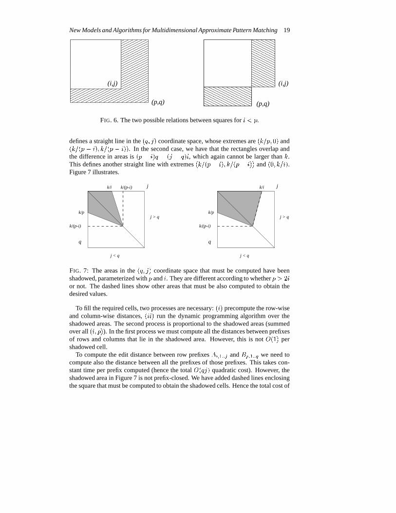
6.1.1 Two DimensionsWe consider which subrectanglesA1::i;1::j andB1::p;1::q are so different that theyneed not be compared becausek insertions are not sufficient to compensate for thedifference in sizes. We consider fixedi andp so thati < p, and study the relevantjandq. The casei > p is symmetric. For fixedi < p there are two different cases:j < q andj � q (see Figure 6).

In the first case, the subrectangle ofA is totally contained in that ofB, and thedifference in areas ispq � ij, which must satisfypq � ij � k. For fixedi andp, this


��

��

��

��

��

��

(p,q)

(i,j) (i,j)

(p,q)

FIG. 6. The two possible relations between squares fori < p.

defines a straight line in the(q; j) coordinate space, whose extremes are(k=p; 0) and(k=(p � i); k=(p � i)). In the second case, we have that the rectangles overlap andthe difference in areas is(p � i)q + (j � q)i, which again cannot be larger thank.This defines another straight line with extremes(k=(p � i); k=(p � i)) and(0; k=i).Figure 7 illustrates.

��

��

j < q

j > q

k/(p-i)

q

j

k/p

k/i k/(p-i)

��

��

j < q

j > q

k/(p-i)

q

j

k/p

k/i

FIG. 7: The areas in the(q; j) coordinate space that must be computed have beenshadowed, parameterized withp andi. They are different according to whetherp > 2ior not. The dashed lines show other areas that must be also computed to obtain thedesired values.

To fill the required cells, two processes are necessary:(i) precompute the row-wiseand column-wise distances,(ii) run the dynamic programming algorithm over theshadowed areas. The second process is proportional to the shadowed areas (summedover all(i; p)). In the first process we must compute all the distances between prefixesof rows and columns that lie in the shadowed area. However, this is notO(1) pershadowed cell.

To compute the edit distance between row prefixesAi;1::j andBp;1::q we need tocompute also the distance between all the prefixes of those prefixes. This takes con-stant time per prefix computed (hence the totalO(qj) quadratic cost). However, theshadowed area in Figure 7 is not prefix-closed. We have added dashed lines enclosingthe square that must be computed to obtain the shadowed cells. Hence the total cost of


the preprocessing is proportional to this extended set of cells, and therefore dominatesthe total processing time.

To measure the area enclosed in dashed lines we must separatethe cases shown inFigure 7, which depend on whetheri < p � 2i or p > 2i. In the first case the totalarea is(k=(p � i))2 and in the secondpk2=(2i(p � i)2). Summing all the relevantareas over1 � i < p � m yieldsO(k2m).6.1.2 More than Two DimensionsWe can generalize the above scheme tod > 2 dimensions. In general, if we havetwo hypercubes, we need to compare them only if they are reasonably close in size.Considering again that the preprocessing that compares allthem2 different(d � 1)-dimensional objects along each dimension is the most expensive part, we see thattwo objects of “volume”V that are at positionsi andp need only be compared ifV (p� i) � k, sinceV (p� i) is the minimum number of insertions necessary to makethem comparable (their volume could be different, sayV1 andV2, but the number ofinsertions ismax(V1; V2)(p�i) and therefore the limit is reached for similar volumes).Comparing those objects of volumeV , together with all their prefixes (objects ofsmaller volume) takesO(V 2), which is limited by(k=(p � i))2). Summing over all(i; p) yieldsO(k2m), and summing this over each dimension givesO(dk2m).7 Multidimensional Searching Algorithms

We first present some new results on exact multidimensional pattern matching whichwe later use for fast filter algorithms for multidimensionalapproximate pattern match-ing.

7.1 Exact Multidimensional Pattern Matching

In [12], they allow searching, in two dimensions, a pattern in a text inO(n2=m)average time. They traverse only the text rows of the formi � m searching for allthe pattern rows at the same time (using Aho-Corasick [1]), and verify all potentialmatches. Clearly, no match can be missed with the filter.

In [12], the authors briefly mention that their technique canbe extended to moredimensions by selecting one dimension and recursively using an algorithm for(d�1)dimensions on them-th “rows” of such text. However no more details are given, norany analysis.

We give now a more detailed version of the algorithm and analyze it. We selectone dimension (say, coordinate 1) and obtainn=m different(d � 1) dimensional ob-jects of the formTm;1::n;1::n;:::, T2m;1::n;1::n;:::, ..., Tim;1::n;1::n;:::, and so on. Onthe other hand, we obtainm patterns of(d � 1) dimensions, namelyP1;1::m;1::m;:::,P2;1::m;1::m;:::, ...,Pp;1::m;1::m;::: and so on. All them subpatterns are searched in eachone of the(d�1) dimensional subtexts. See Figure 8. Each time one of the(d�1) di-mensional subpatterns is found in a text position, the completed-dimensional pattern


2-d text

2-d pattern

2-d pattern

3-d text3-d pattern

3-d pattern

FIG. 8: Algorithm for exact searching. All the pattern “rows” are searched inn=mtext “rows” at the same time.

is checked.An important part of the analysis of [12] for two dimensions is that the total cost to

verify potential matches is not too large. It is not immediate that this is still valid formore dimensions, since a very large number of verifications are finally triggered.

The cost to verify a potential match ind dimensions is alwaysO(1) on average,since we have to check ifmd letters of the pattern are equal to the text at a givenposition. Since we stop the checking as soon as we find a mismatch, we verify morethan characters with probability1=� . Hence, the average number of characterschecked is

P 1=� = O(1) (even for patterns of unbounded size).We denote byEd;r the average search cost forr patterns ind dimensions. The

existence of the Aho-Corasick [1] algorithm implies thatE1;r = n. Now, for d di-mensions, we performn=m searches forrm patterns ond� 1 dimensions, and checkall the candidates that occur. The probability of a pattern of sizemd�1 occurring ina text position is1=�md�1

, but we multiply that byrm because we search forrmdifferent patterns. As the average cost to verify each potential match isO(1), and the(d� 1) dimensional texts are of sizend�1, we have thatEd;r = nm �Ed�1;rm + nd�1 rm�md�1 � = nmEd�1;rm + ndr�md�1which givesEd;r = ndmd�1 + d�1Xw=1 ndr�mw = O�nd � 1md�1 + r�m��(where the first term corresponds to the actual searches which are all done in onedimension).

To search for one pattern we replacer by 1 in this final formula (although thealgorithm internally uses multipattern search). This formula matches the result fortwo dimensions, since1=�m = o(1=m). In general, ifd is considered fixed, the


3 dimensions1 dimension

2 dimensions

FIG. 9: Filtering algorithm forj = 3. The maximum possiblek so that some blockappears unchanged is 2, 2, and 8 as the dimension grows.

above result forr = 1 can be bounded byO(nd=md�1). The worst case search costcorresponds to verifying all text positions like a brute force search, i.e.O(rmdnd).

The space complexity of the algorithm corresponds to the Aho-Corasick machine,whose space requirements are proportional to the total sizeof all the patterns, i.e.O(rmd). We use this algorithm as a building block in the next section.

7.2 A Fast Filter for Multidimensional Approximate Searching

We present now an effective filter to quickly discard large parts of the text whichcannot contain a match, so that we use the dynamic programming algorithm to verifyonly the text areas which could contain an occurrence of the pattern.

The filter is based on a generalization of the one-dimensional filter explained inSection 2. In that case, we cut the pattern in(k + 1) pieces, and since each errorcan destroy at most one piece, we have always one piece left untouched inside eachoccurrence.

In two and more dimensions, we cut the pattern inj pieces along each dimension,for some1 � j � m (see Figure 9). Since each error occurs along one dimensiononly, at mostkj pieces are destroyed. Therefore, since there arejd pieces in total,it is enough thatjd > kj to ensure that at least one of the pieces is left untouched(although we do not know which one). Hence, we search for all thejd pieces at thesame time in the text without allowing errors. Those pieces are of size(m=j)d, andcan be searched with the algorithm of the previous section inO(md) space and an


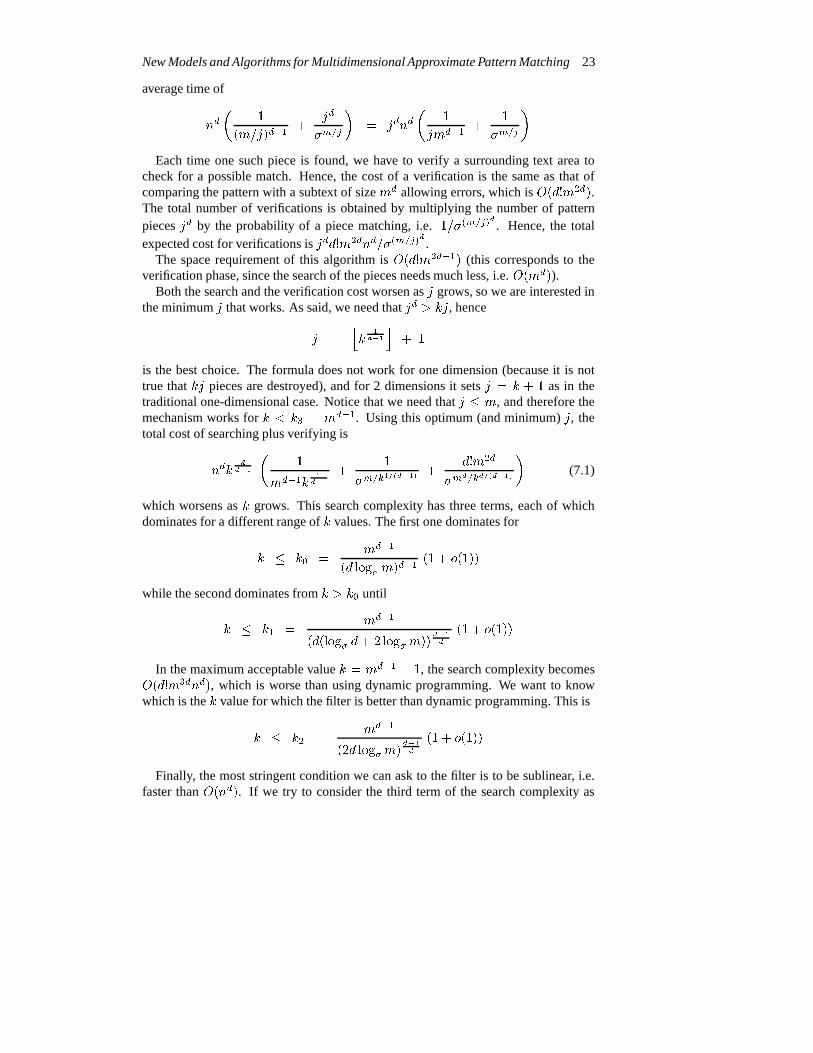
average time ofnd� 1(m=j)d�1 + jd�m=j� = jdnd� 1jmd�1 + 1�m=j �Each time one such piece is found, we have to verify a surrounding text area to

check for a possible match. Hence, the cost of a verification is the same as that ofcomparing the pattern with a subtext of sizemd allowing errors, which isO(d!m2d).The total number of verifications is obtained by multiplyingthe number of patternpiecesjd by the probability of a piece matching, i.e.1=�(m=j)d . Hence, the totalexpected cost for verifications isjdd!m2dnd=�(m=j)d .

The space requirement of this algorithm isO(d!m2d�1) (this corresponds to theverification phase, since the search of the pieces needs muchless, i.e.O(md)).

Both the search and the verification cost worsen asj grows, so we are interested inthe minimumj that works. As said, we need thatjd > kj, hencej = jk 1d�1 k + 1is the best choice. The formula does not work for one dimension (because it is nottrue thatkj pieces are destroyed), and for 2 dimensions it setsj = k + 1 as in thetraditional one-dimensional case. Notice that we need thatj � m, and therefore themechanism works fork < k3 = md�1. Using this optimum (and minimum)j, thetotal cost of searching plus verifying isndk dd�1 � 1md�1k 1d�1 + 1�m=k1=(d�1) + d!m2d�md=kd=(d�1) � (7.1)

which worsens ask grows. This search complexity has three terms, each of whichdominates for a different range ofk values. The first one dominates fork � k0 = md�1(d log� m)d�1 (1 + o(1))while the second dominates fromk > k0 untilk � k1 = md�1(d(log� d+ 2 log�m)) d�1d (1 + o(1))

In the maximum acceptable valuek = md�1 � 1, the search complexity becomesO(d!m3dnd), which is worse than using dynamic programming. We want to knowwhich is thek value for which the filter is better than dynamic programming. This isk � k2 = md�1(2d log�m) d�1d (1 + o(1))

Finally, the most stringent condition we can ask to the filteris to be sublinear, i.e.faster thanO(nd). If we try to consider the third term of the search complexityas


dominant, we arrive to ak value which is smaller thank1, which means that the solu-tion is in a stricterk range. By considering the second term of the search complexity,we arrive to the conditionk � k0. That is, the search time is sublinear precisely whenthe first term of the summation dominates.

To summarize, the search algorithm is sublinear (i.e.O(knd=md�1)) for k <(m=(d log�m))d�1. Otherwise, it is not sublinear, but it improves over dynamic pro-gramming fork � md�1=(2d log�m)(d�1)=d. Figure 10 illustrates the result of theanalysis.

0

Dyn. prog.

k

third termsecond term

Filter

k k k k0 1 2 3

O(n )d

dominatesfirst term

dominates dominates

FIG. 10. The complexity of the proposed filter, depending onk.

7.3 A Stricter Filter

We have assumed up to now that we verify the presence of the pattern allowing errorsas soon as any of thejd pieces appears. However, we can do better. We know thatjd � jk pieces must appear, at their correct positions, for a match to be possible.Therefore, whenever a piece appears, we can check the neighborhood for the exactoccurrences of other pieces. On average, the verification ofeach piece will fail inO(1)character comparisons, and we will checkO(jk) pieces untiljk of them fail the test(this is because both are geometric processes). Therefore,we have a preverificationtest which occurs with probabilityjd=�(m=j)d , costsO(jk) and is able to discardmore text positions before actually verifying the candidate area. The probability that atext position passes the preverification test and undergoesthe dynamic programmingverification can be computed by considering thatjd � jk cells need to match, whichmeans thatmd�kmd=jd�1 characters match. On the other hand, we can select as wewant whichjk cells match out ofjd.


The new search cost is thereforend0� jd�1md�1 + jd�m=j + jdjk�(m=j)d + �jdjk�d!m2d�md�kmd=jd�11Awhere the first term dominates forj � m=(d log� m), the second one up toj �m=(log�m + log� k)1=d, and the third one for largerj. The fourth term decreaseswith j, and therefore it is not immediate that the minimumj is the optimum (in factit is not). We have not been able to determine the optimumj, but we can still obtainthe maximumk value up to where the filter is better than dynamic programming. Thefirst two terms are never worse than dynamic programming, andthe third improvesover dynamic programming forj � m(log�m+ log� k � d log� d)1=d (1 + o(1))which gives a condition onk sincejd�1 > k:k � k02 = md�1(d(log�m� log� d)) d�1d (1 + o(1))

Now, we introduce this maximumj value in the fourth term to determine whetherit is also better than dynamic programming at that point. Theresult is that, using thatj value, the fourth term is dominated by the third precisely for k � k02. Therefore weimprove over dynamic programming fork � k02 (which is better than our previousk2limit). The proposedj is the best for highk values, but smaller values are better forlowerk values. In particular, we may be interested in obtaining thesublinearity limitfor this filter. The first three terms put an upper bound onj, the strictest one beingj � md(log� m� log� d) (1 + o(1))and using this maximumj value the fourth term gives us the maximumk that allowssublinear search time:k � k00 = md�1(d(log�m� log� d))d�1 (1 + o(1))which is slightly better than our previousk0 limit.

We could have used the algorithm of Karkkainen and Ukkonen[22] instead of thatof Baeza-Yates and Regnier [12] considering that the former is faster on average.However, the former does not have the ability of searching many patterns simultane-ously, which is the key issue in our case. In fact, using that algorithm, our filter isslower only in two cases:

i) k < � md2d+1 log�m� d�1d+1which is a very smallk; or

ii) k � md�1, which is too large and where the filters do not work anyway.

This resembles the difference between searching multiple patterns using a Boyer-Moore or an Aho-Corasick algorithm.


7.4 Adapting the Filter to Simpler Distances

Since theR andC distances are lower bounded byRC, the filter we have just designedfor RC works forR andC as well, with the same complexities (albeit only the cased = 2 is interesting).

Another possible simplification is to use the filter to searcha pattern allowingksubstitutions. This problem is much simpler: a brute force search algorithm checksany possible text position until it findsk mismatches. Being a geometric process, thisoccurs afterO(k) character comparisons, which makes the total search costO(knd)on average.

Therefore, in this model the cost to verify a candidate text position is onlyO(k).The search cost, as in Eq. (7.1), still has three terms:ndk dd�1 � 1md�1k 1d�1 + 1�m=k1=(d�1) + k�md=kd=(d�1) �where the first term is dominant fork � k0. The second term is now dominant fork � k01 = md�1(d log�m) d�1d (1 + o(1))and the last one dominates fork > k01. This filter is sublinear (i.e. does not inspectall the text characters) on average fork < k0 as before. On the other hand, it turnsout to be better than brute force (i.e.O(knd)) for k � k01, i.e. before the verificationstep dominates the search cost. Overall, we achieve theO(knd=md�1) search time onaverage. However, Karkkainen and Ukkonen algorithm’s [22] for this case is faster,achievingO(dndk log�(m)=md) average time.

8 Concluding Remarks

We have focused on two and multidimensional approximate pattern matching. Thecontribution of this work is many fold. We have developed thefirst sublinear averagetime filters for the existing model on two dimensions. We haveproposed new distancesfor two dimensions and have shown how to compute them and how to search a patternin a text under those distances. The most promising of them, that we have called theRC distance, allows the errors to occur along rows and columns at any time. Wehave generalized the most promising of them tod dimensions and have presented ad-dimensional filtering algorithm that yields sublinear search time when the error leveltolerated is low enough. For instance, in two dimensions thefilter is sublinear time fork < m=(2 log� m) and better than a brute force search fork � m=p2 log� m.

These are the first search algorithms and fast filters for the first model which extendssuccessfully the concept of approximate string matching tomore than one dimension.Although the algorithms have been presented for squared-dimensional pattern andtext, they also work for hyper-rectangular elements and more complex shapes.

An open problem is how to design optimal worst-case time algorithms for approx-imate searching using the new measures, i.e. achievingO(m2n2) time complexity


for theR, C, L, andRC measures. Another interesting problem is how to searchefficiently using theL distance.

There are other open problems related to the models themselves. For example,we could try to define thelargest common imageof two images, which generalizesthe concept of longest common subsequence of one-dimensional strings. Given twoimages, find a set of position pairs that match exactly in bothimages subject to thefollowing restrictions:

1. The set of positions for the same pattern are disjoint;

2. a suitable order given by the position values is the same for both images (forexample, image pixels can be sorted by theiri + j value, using the value ofiin the case of ties); and

3. the total size of the set of positions is maximized.

For the edit distance, condition 3 has to be changed to:

3. Minimize the number of mismatches, insertions and deletions needed to obtain theset of matching positions.

Figure 11 gives an example. All pieces of the pattern not in the text correspondsto deletions and mismatches and should be counted. In the text, black regions are notcounted, because they correspond to mismatches. All other pieces are insertions in thepattern. It is not clear that the minimal string editing solution gives the same answeras the largest common set of sub-images. Also, it could be argued that charactersinserted/deleted on external borders should not be countedas errors.

��

��

��

��

��

��

��

��

��

��

��

��

4��

��

��

��

��

Pattern Text piece

1 1

2

34 3

2

FIG. 11. Example of largest common image.

The approximate two-dimensional pattern matching problemcan be stated as usualusing the above definition as searching for all rectangular subimages of the text thathave edit distance at mostk with the pattern. An alternative definition would be tofind all pieces of the text that have at leastm2�k matching positions with the pattern.

Our work is a (very preliminary) step towards presenting a combinatorial alternativeto the current image processing technology. Other related approaches have focused onrotations [20] and scalings [3, 2] An open problem is how to combine those approachesto allow deformations in the occurrences.


Acknowledgements

We would like to thank the comments of Sven Schuerier regarding the new models(which in particular pointed out the simplification for computing theL measure).

References[1] A. Aho and M. Corasick. Efficient string matching: an aid to bibliographic search.CACM, 18(6):333–

340, June 1975.[2] A. Amir, A. Butman, and M. Lewenstein. Real scaled matching. InProc. SODA 2000, page To appear.,

San Francisco, January 2000.[3] A. Amir and G. Calinescu. Alphabet independent and dictionary scaled matching. InProc. CPM’96,

number 1075 in LNCS, pages 320–334, 1996.[4] A. Amir and M. Farach. Efficient 2-dimensional approximate matching of non-rectangular figures. In

Proc. SODA’91, pages 212–223, 1991.[5] A. Amir and G. Landau. Fast parallel and serial multidimensional approximate array matching.The-

oretical Computer Science, 81:97–115, 1991.[6] M. Atallah. A linear time algorithm for the Hausdorff distance between convex polygons.Information

Processing Letters, 17:207–209, 1983.[7] R. Baeza-Yates. Similarity in two-dimensional strings. In Proc. COCOON’98, number 1449 in LNCS,

pages 319–328, Taipei, Taiwan, August 1998.[8] R. Baeza-Yates and G. Navarro. Multiple approximate string matching. InProc. WADS’97, LNCS

1272, pages 174–184, 1997.[9] R. Baeza-Yates and G. Navarro. Fast two-dimensional approximate pattern matching. InProc.

LATIN’98, number 1380 in LNCS, pages 341–351. Springer-Verlag, 1998.[10] R. Baeza-Yates and G. Navarro. Faster approximate string matching.Algorithmica, 23(2):127–158,

1999.[11] R. Baeza-Yates and C. Perleberg. Fast and practical approximate pattern matching. InProc. CPM’92,

LNCS 644, pages 185–192, 1992.[12] R. Baeza-Yates and M. Regnier. Fast two dimensional pattern matching. Information Processing

Letters, 45:51–57, 1993.[13] T. Baker. A technique for extending rapid exact string matching to arrays of more than one dimension.

SIAM Journal on Computing, 7:533–541, 1978.[14] R. Bird. Two dimensional pattern matching.Inf. Proc. Letters, 6:168–170, 1977.[15] B. Commentz-Walter. A string matching algorithm fast on the average. InProc. ICALP’79, number 6

in LNCS, pages 118–132. Springer-Verlag, 1979.[16] M. Crochemore and W. Rytter.Text Algorithms. Oxford University Press, Oxford, UK, 1994.[17] C. Faloutsos, R. Barber, M. Flickner, J. Hafner, W. Niblack, D. Petkovic, and W. Equitz. Efficient and

effective querying by image content.J. of Intelligent Information Systems, 3:231–262, 1994.[18] K. Fredriksson, G. Navarro, and E. Ukkonen. Fast filtersfor two dimensional string matching allowing

rotations. Technical Report TR/DCC-99-9, Dept. of Computer Science, Univ. of Chile, November1999.

[19] K. Fredriksson, G. Navarro, and E. Ukkonen. An index fortwo dimensional string matching allowingrotations. Technical Report TR/DCC-99-8, Dept. of Computer Science, Univ. of Chile, November1999. Submitted toIFIP TCS 2000.

[20] K. Fredriksson and E. Ukkonen. A rotation invariant filter for two-dimensional string matching. InProc. CPM’98, number 1448 in LNCS, pages 118–125, 1998.

[21] R. Giancarlo. A generalization of suffix trees to squarematrices, with applications.SIAM J. onComputing, 24:520–562, 1995.

[22] J. Karkkainen and E. Ukkonen. Two and higher dimensional pattern matching in optimal expectedtime. InProc. SODA’94, pages 715–723. SIAM, 1994.


[23] K. Krithivasan. Efficient two-dimensional parallel and serial approximate pattern matching. TechnicalReport CAR-TR-259, University of Maryland, 1987.

[24] K. Krithivasan and R. Sitalakshmi. Efficient two-dimensional pattern matching in the presence oferrors.Information Sciences, 43:169–184, 1987.

[25] R. Muth and U. Manber. Approximate multiple string search. In Proc. CPM’96, LNCS 1075, pages75–86, 1996.

[26] G. Navarro. Multiple approximate string matching by counting. InProc. WSP’97, pages 125–139,1997.

[27] G. Navarro. A guided tour to approximate string matching. Technical Report TR/DCC-99-5, Dept.of Computer Science, Univ. of Chile, 1999. To appear inACM Computing Surveys. ftp://-ftp.dcc.uchile.cl/pub/users/gnavarro/survasm.ps.gz.

[28] G. Navarro and R. Baeza-Yates. Fast multi-dimensionalapproximate string matching. InProc.CPM’99, LNCS v. 1645, pages 243–257, 1999.

[29] S. Needleman and C. Wunsch. A general method applicableto the search for similarities in the aminoacid sequences of two proteins.J. of Molecular Biology, 48:444–453, 1970.

[30] K. Park. Analysis of two dimensional approximate pattern matching algorithms. InProc. CPM’96,LNCS 1075, pages 335–347, 1996.

[31] S. Ranka and T. Heywood. Two-dimensional pattern matching withk mismatches.Pattern recognition,24(1):31–40, 1991.

[32] P. Sellers. The theory and computation of evolutionarydistances: pattern recognition.J. of Algorithms,1:359–373, 1980.

[33] P. Suetens, P. Fua, and A. Hanson. Computational strategies for object recognition.ACM ComputingSurveys, 24:5–62, 1992.

[34] S. Wu and U. Manber. Fast text searching allowing errors. CACM, 35(10):83–91, October 1992.[35] R. Zhu and T. Takaoka. A technique for two-dimensional pattern matching.Comm. ACM, 32(9):1110–

1120, 1989.

new models and algorithms for multidimensional approximate

Documents