new results on the resistivity structure of merapi volcano (indonesia

Geophys. J. Int. (2006) 167, 1172–1187 doi: 10.1111/j.1365-246X.2006.03182.xG

JIG

eom

agne

tism

,ro

ckm

agne

tism

and

pala

eom

agne

tism

New results on the resistivity structure of Merapi Volcano(Indonesia), derived from three-dimensional restricted inversionof long-offset transient electromagnetic data

Michael Commer,1 Stefan L. Helwig,2 Andreas Hordt,3 Carsten Scholl4

and Bulent Tezkan2

1Earth Sciences Division, Lawrence Berkeley National Laboratory, Berkeley, CA, USA. E-mail: [email protected] of Geophysics and Meteorology, University of Cologne, Cologne, Germany3Institute of Geophysics and Extraterrestrial Physics, Technical University of Braunschweig, Braunschweig, Germany4Department of Physics, University of Toronto, Toronto, ON, Canada

Accepted 2006 August 10. Received 2006 August 10; in original form 2005 October 14

S U M M A R YThree long-offset transient electromagnetic (LOTEM) surveys were carried out at the activevolcano Merapi in Central Java (Indonesia) during the years 1998, 2000 and 2001. The mea-surements focused on the general resistivity structure of the volcanic edifice at depths of 0.5–2 km and the further investigation of a southside anomaly. The measurements were insufficientfor a full 3-D inversion scheme, which could enable the imaging of finely discretized resistiv-ity distributions. Therefore, a stable, damped least-squares joint-inversion approach is used tooptimize 3-D models with a limited number of parameters. The models feature the realisticsimulation of topography, a layered background structure, and additional coarse 3-D blocksrepresenting conductivity anomalies. 28 LOTEM transients, comprising both horizontal andvertical components of the magnetic induction time derivative, were analysed. In view of thefew unknowns, we were able to achieve reasonable data fits. The inversion results indicatean upwelling conductor below the summit, suggesting hydrothermal activity in the centralvolcanic complex. A shallow conductor due to a magma-filled chamber, at depths down to1 km below the summit, suggested by earlier seismic studies, is not indicated by the inversionresults. In conjunction with an anomalous-density model, derived from a recent gravity study,our inversion results provide information about the southern geological structure resulting froma major sector collapse during the Middle Merapi period, approximately 14 000 to 2200 yr BP.The density model allows to assess a porosity range and thus an estimated vertical salinityprofile to explain the high conductivities on a larger scale, extending beyond the foothills ofthe volcano.

Key words: Merapi volcano, 3-D least squares inversion, transient electromagnetic fields.

1 I N T RO D U C T I O N

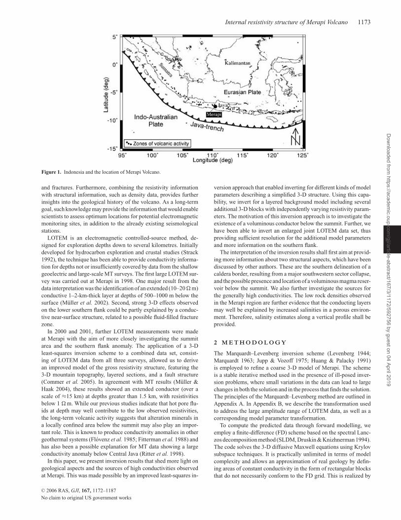
The Indonesian volcano Merapi, in the eastern part of Central Java,

is one of the most active volcanoes on Earth. As shown in Fig. 1,

it is located over the subduction zone between the Eurasian and

Indo-Australian Plates. Classified as a high-risk volcano, the most

recent activity in 2006 has again shown the permanent danger to life

within Merapi’s densely populated surroundings. Over more than

60 yr, the frequent activity has been systematically observed in or-

der to improve the understanding of eruption history and complex

internal processes. Since 1980, international cooperation has in-

creased, enhancing observation capabilities. Under the leadership of

the German Geo-Forschungs-Zentrum Potsdam, and in cooperation

with the Volcanological Survey of Indonesia (VSI) and other institu-

tions of Indonesia and Germany, a large interdisciplinary monitoring

programme was initiated in 1994 (Zschau et al. 1998). Because as-

sessing volcanic activity parameters is an important requirement

for improving prediction capabilities, one main project goal was

the multidisciplinary investigation of the volcano’s edifice struc-

ture. Electromagnetic methods were employed because of the typ-

ically high resistivity contrasts in volcanoes, caused by resistive

host rock, conductive magma reservoirs, and associated hydrother-

mal systems (Jackson & Keller 1972; Fitterman et al. 1988; Lenat

et al. 2001). Measurements using geoelectric (Friedel et al. 2000),

magnetotelluric (MT, Muller & Haak 2004), and long-offset tran-

sient electromagnetic (LOTEM, Muller et al. 2002; Commer et al.2005) methods were made with the aim of relating Merapi’s resis-

tivity distribution to important factors such as temperature, porosity

1172 C© 2006 RAS

No claim to original US government works

Dow

nloaded from https://academ

ic.oup.com/gji/article-abstract/167/3/1172/592756 by guest on 04 April 2019

Internal resistivity structure of Merapi Volcano 1173

Figure 1. Indonesia and the location of Merapi Volcano.

and fractures. Furthermore, combining the resistivity information

with structural information, such as density data, provides further

insights into the geological history of the volcano. As a long-term

goal, such knowledge may provide the information that would enable

scientists to assess optimum locations for potential electromagnetic

monitoring sites, in addition to the already existing seismological

stations.

LOTEM is an electromagnetic controlled-source method, de-

signed for exploration depths down to several kilometres. Initially

developed for hydrocarbon exploration and crustal studies (Strack

1992), the technique has been able to provide conductivity informa-

tion for depths not or insufficiently covered by data from the shallow

geoelectric and large-scale MT surveys. The first large LOTEM sur-

vey was carried out at Merapi in 1998. One major result from the

data interpretation was the identification of an extended (10–20� m)

conductive 1–2-km-thick layer at depths of 500–1000 m below the

surface (Muller et al. 2002). Second, strong 3-D effects observed

on the lower southern flank could be partly explained by a conduc-

tive near-surface structure, related to a possible fluid-filled fracture

zone.

In 2000 and 2001, further LOTEM measurements were made

at Merapi with the aim of more closely investigating the summit

area and the southern flank anomaly. The application of a 3-D

least-squares inversion scheme to a combined data set, consist-

ing of LOTEM data from all three surveys, allowed us to derive

an improved model of the gross resistivity structure, featuring the

3-D mountain topography, layered sections, and a fault structure

(Commer et al. 2005). In agreement with MT results (Muller &

Haak 2004), these results showed an extended conductor (over a

scale of ≈15 km) at depths greater than 1.5 km, with resistivities

below 1 � m. While our previous studies indicate that hot pore flu-

ids at depth may well contribute to the low observed resistivities,

the long-term volcanic activity suggests that alteration minerals in

a locally confined area below the summit may also play an impor-

tant role. This is known to produce conductivity anomalies in other

geothermal systems (Flovenz et al. 1985; Fitterman et al. 1988) and

has also been a possible explanation for MT data showing a large

conductivity anomaly below Central Java (Ritter et al. 1998).

In this paper, we present inversion results that shed more light on

geological aspects and the sources of high conductivities observed

at Merapi. This was made possible by an improved least-squares in-

version approach that enabled inverting for different kinds of model

parameters describing a simplified 3-D structure. Using this capa-

bility, we invert for a layered background model including several

additional 3-D blocks with independently varying resistivity param-

eters. The motivation of this inversion approach is to investigate the

existence of a voluminous conductor below the summit. Further, we

have been able to invert an enlarged joint LOTEM data set, thus

providing sufficient resolution for the additional model parameters

and more information on the southern flank.

The interpretation of the inversion results shall first aim at provid-

ing more information about two structural aspects, which have been

discussed by other authors. These are the southern delineation of a

caldera border, resulting from a major southwestern sector collapse,

and the possible presence and location of a voluminous magma reser-

voir below the summit. We also further investigate the sources for

the generally high conductivities. The low rock densities observed

in the Merapi region are further evidence that the conducting layers

may well be explained by increased salinities in a porous environ-

ment. Therefore, salinity estimates along a vertical profile shall be

provided.

2 M E T H O D O L O G Y

The Marquardt–Levenberg inversion scheme (Levenberg 1944;

Marquardt 1963; Jupp & Vozoff 1975; Huang & Palacky 1991)

is employed to refine a coarse 3-D model of Merapi. The scheme

is a stable iterative method used in the presence of ill-posed inver-

sion problems, where small variations in the data can lead to large

changes in both the solution and in the process that finds the solution.

The principles of the Marquardt–Levenberg method are outlined in

Appendix A. In Appendix B, we describe the transformation used

to address the large amplitude range of LOTEM data, as well as a

corresponding model parameter transformation.

To compute the predicted data through forward modelling, we

employ a finite-difference (FD) scheme based on the spectral Lanc-

zos decomposition method (SLDM, Druskin & Knizhnerman 1994).

The code solves the 3-D diffusive Maxwell equations using Krylov

subspace techniques. It is practically unlimited in terms of model

complexity and allows an approximation of real geology by defin-

ing areas of constant conductivity in the form of rectangular blocks

that do not necessarily conform to the FD grid. This is realized by

C© 2006 RAS, GJI, 167, 1172–1187


Dow



1174 M. Commer et al.

Figure 2. Modelling of the terrain structure with vertical columns. The figure in the upper right corner illustrates the two-layer design that follows the

topography.

a material averaging scheme to calculate the underlying effective

medium (Moskow et al. 1999) and makes the code appropriate for

the implementation of arbitrary model parameters.

Convergence characteristics of SLDM, as described by Druskin

& Knizhnerman (1994), must be taken into account when designing

an FD discretization. In principle, for a given FD grid and earth

model, the stability of SLDM depends on both the latest transient

times to be simulated and the highest conductivity contrasts in a

model. Since simulating arbitrary topography requires accounting

for the air layer in the discretization grid, the difficulty lies in the

high resistivity contrast between the air and the earth, along with

the requirement for a rectilinear FD grid. Using the SLDM code,

Hordt & Muller (2000) carried out extensive studies on the sim-

ulation of LOTEM with topography effects. Here, following their

results, we make sure that a contrast of 100:1 (air:earth) is kept

during an inversion, providing stable and realistic results. This has

been accomplished by carrying out preliminary test inversions and

fixing the air-layer conductivity accordingly. We employ a total of

five different FD grids for the calculation of the data predictions,

to account for different LOTEM transmitters and the large spatial

distances between the receiver positions. The grids are adapted in

both their size and grid spacing to the different transmitter–receiver

configurations and to the measurement time ranges. The difficulty

one has with the SLDM scheme in the presence of long time ranges

is addressed by using separate FD grids, for early and late simula-

tion times. To ensure stability when the material properties change

during the inversion, each grid’s response is tested for consistency

against varying model contrasts in a preliminary forward modelling

study. For more details on the grid verification procedure, the reader

is referred to Hordt & Muller (2000) and Commer (2003).

In contrast to large-scale inversions, where a model is usually

discretized into numerous grid cells, our model is described by only

as many parameters as is typical for Marquardt inversions, usually

less than 10. Hence, we construct a 3-D model featuring rather un-

conventional types of model parametrizations. Fig. 2 illustrates how

the topography of Mt. Merapi is approximated by vertical columns

that are more conductive than the resistive air space. The upward

extension of each column is derived from a digital elevation model

of Merapi (Gerstenecker et al. 1998). The column diameters are

varied such that the discretization is fine at the upper flanks, where

the terrain is very steep, while at greater distances the model be-

comes coarser. To model the regular cone shape of the edifice, the

column’s base areas are square. Based on earlier studies, we assume

a layered background model with the layer boundaries conforming

to the topography. Comparative model studies indicated that such a

dome-shaped structure provides for much better data fits than a hor-

izontally layered background (Commer 2003). The layered model

involves two types of parameters. Similar to 1-D inversions, they

are given by both the thickness and resistivity of each layer. Note,

however, that here the parameters describe a 3-D model of non-

horizontal layers. The upper corner of Fig. 2 exemplifies how a

two-layer background is realized in the model construction proce-

dure. Starting from its upper end, at the air–earth interface, each

column is subdivided according to the (global) thicknesses as many

times as there are layers. Each layer is specified by a resistivity and

thickness, here �1 and d1 for layer 1. The bottom layer, here layer

2, has infinite thickness and thus only a resistivity parameter (�2).

Note that the parameters are equal for each column block within a

given layer.

We further employ an additional type of model parameter that

specifies single 3-D blocks embedded into the background. The

SLDM code does not allow overlapping model blocks. Therefore,

the columns overlapped by the additional structures are further sub-

divided and reshaped into smaller parts, such that an empty space,

C© 2006 RAS, GJI, 167, 1172–1187


Dow




conforming to the new block, is formed. In practice, this process

is repeated for each additional block. In principle, the scheme al-

lows the creation of arbitrary 3-D shapes that can be cast into model

unknowns. However, as dictated by the least-squares method, the

inversion is constrained by a limited number of model parameters,

a maximum number of eight in this work.

3 G E O L O G I C A L B A C KG RO U N D

Merapi is a basalt-to-basaltic-andesite volcanic complex with a max-

imum elevation of 2911 m above sea level. Modern studies of the ge-

ological evolution of Merapi started with Van Bemmelen (1949). He

introduced the scenario of an eroded older volcanic edifice, which

began to grow during the Pleistocene. This so-called Old Merapi

consists of a sequence of basaltic andesite lavas and intercalated

pyroclastic deposits, and is overlain by the deposits of a younger

volcanic cone (New Merapi) (Newhall et al. 2000). Fig. 3 depicts

the major geological features. The growth of the volcano was in-

terrupted several times by violent magmatic to phreatomagmatic

eruptions and one or possibly several Mount St Helens-type edifice

collapses in the southwestern section during the so-called Middle

Merapi period, 14 000 to 2200 yr BP (Camus et al. 2000; Newhall

et al. 2000; Gertisser 2001). These events left a horseshoe-shaped

morphology of the older volcanic cone and may have sent large

debris avalanches down the western slopes. The edge of the sector

collapses, pointed out by Van Bemmelen (1949) as a ‘hyperbolic

fault’ (dashed line in Fig. 3), was later related to an avalanche

caldera rim with a wider opening angle than supposed by Van

Bemmelen (Camus et al. 2000). Aside from the remnants of the

older eruptive stages, much of the area surrounding the volcanic

complex is covered by Holocene pyroclastic deposits, forming an

Figure 3. Geological sketch map of the Merapi region, after Gertisser (2001), based on Van Bemmelen (1949). The lower figure shows a section through the

western sector of the volcano (profile line). The horizontal dotted line shows the location of the section border in our model results at ∼7 km south of the

summit.

extensive apron around the volcano (Gertisser & Keller 2003). The

material below the volcanic deposits was identified as low-density

Cenozoic sediments, as indicated by gravity measurements (Natori

1978; Tiede et al. 2005). Earlier, Van Bemmelen (1949) identified

the basement sediments as marine Tertiary formations and cites an

incomplete consolidation of the ‘plastic marine strata’ as evidence

of the volcano–tectonic collapse. Presently, the volcanic activity is

characterized by the extrusion of viscous lavas forming domes in the

summit area. The collapse of these lava domes due to gravitational

instability causes small-volume pyroclastic flows (nuees ardentes)

at regular intervals of a few years.

3.1 A priori geophysical information

To characterize the electrical structure, DC resistivity soundings

on the upper flanks (Friedel et al. 2000) and large-scale MT and

geomagnetic induction vector measurements (Muller & Haak 2004)

were carried out at Merapi. These methods and the LOTEM results

(Muller et al. 2002; Commer et al. 2005) indicated that the resistivity

distribution in the upper kilometre reflects the volcanic stratigraphy.

The DC resistivity soundings are capable of resolving the upper few

hundred metres. On the western and southern flank, the soundings

show resistivities above 1000 � m within the first 200–300 m, which

drop rapidly to values below 100 and 10 � m, respectively, to a

resolved depth of ≈800 m. Other volcanological resistivity studies,

for example at Newberry Volcano (Oregon) (Fitterman et al. 1988)

or Piton de la Fournaise (Reunion Island) (Lenat et al. 2001), also

showed that resistivities are usually high at shallow depths. Friedel

et al. (2000) suggested that the decrease of resistivity below 50 � m

might indicate the upper zone of a hydrothermal system below the

summit, rather than freshwater saturation of the pyroclastic deposits.

C© 2006 RAS, GJI, 167, 1172–1187


Dow




Figure 4. Vertical cross-section through the summit from the 3-D model

derived from MT measurements (after Muller & Haak 2004). Structures:

(A) Upper layer (100 � m), (B) Intermediate conducting layer (10 � m),

(C) Conducting layer (1 � m), (D) Central conductor (10 � m), (E) SW

anomaly (1 � m) and (F) Two extended conductors (0.1 � m). The dashed

line indicates the position of the fault dividing the layered model in our

results.

All methods identified a generally strong resistivity decrease with

depth. While the exploration depth of the DC soundings is limited,

the MT data allowed the resolution of structures at maximum depths

of ≈1800 m below sea level, as shown by the 3-D modelling results

in Fig. 4. The model is characterized by several layers with a 1 � m

conducting bottom layer (C) at 0.4–1.8 km, while at larger depths a

resistivity increase is indicated by the data (Muller & Haak 2004).

According to Muller & Haak, the intermediate (10 � m) conducting

layer (B) and the central conductor (D) are necessary to explain the

magnitudes of induction vectors at 1700–2000 m above sea level,

although a finer structure could not be resolved. Here, we show that

the LOTEM data provide important additional information for this

region of interest, due to the smaller exploration depth focusing on

0.5–2 km below the surface.

The lateral position of the deep west–east striking anomaly on the

southern flank (Structure F in Fig. 4) is possibly connected to the

conductivity anomalies identified by the LOTEM data in this area

(Muller et al. 2002; Kalscheuer et al. 2004; Commer et al. 2005).

Model studies have already suggested a vertical fault structure at a

position depicted by the dashed line in Fig. 4. We will show further

evidence for such a structure, which can possibly be related to the

boundaries of the edifice collapse during the Middle Merapi period.

The interpretation of the inversion results in this work is greatly

improved in terms of ambiguity by including the results of a recent

gravity inversion study (Tiede et al. 2005). In that study, a subsurface

3-D density model of the Merapi and Merbabu region was derived

by inversion of data from 443 gravity stations. The results further

confirm the relatively low rock densities in the Merapi region. Using

a least-squares inversion approach, a mean density of 2241 kg m−3

and maximal density anomalies between −242 and +264 kg m−3

were found. To explain these densities, Tiede et al. (2005) infer a

porosity range of 10–20 per cent.

4 T H E L O T E M DATA

The joint LOTEM data set comprises two different transmitters and

24 receiver stations. The transmitters consisted of long (1–2 km)

horizontal electric dipoles (HED), injecting a square wave current

into the ground. A Zonge GGT10 transmitter with 10 kVA power

generator supplied the input current, which was injected through

steel pipes. The data acquisition was performed using the TEAMEX

and SUMMIT measurement systems, originally seismic equipment

specially modified for TEM measurements (Ruter & Strack 1991).

Both systems are multichannel remote unit systems that are digitally

connected to a data-recording PC. A single raw transient is usually

dominated by 50 Hz (and multiples) power-line noise. Therefore,

we collected up to several thousand transients at each station to

provide for a sufficient signal-to-noise ratio. They were digitally

filtered, using techniques described by Hanstein (1996), and selec-

tively stacked. The uncertainties used for weighting each datum are

given by the standard deviation of the distribution resulting from

the stacking process.

Fig. 5(a) presents an overview of all stations comprising the joint

data set. Stations 1–6 were recorded in 1998, and the measurement

at Station 1 was repeated in 2000 with the SUMMIT equipment,

enabling longer recording times and thus a larger depth of inves-

tigation. The corresponding transmitter HED-1 was a grounded

1-km-long wire, located to the north, approximately 4 km from

the summit and at an elevation of 1500 m above sea level. The sum-

mit Station 1b and Stations 20–49, referred to as southern profile

in the following, were measured during 2001. These stations were

generated by the 2 km long transmitter HED-2, located at 530 m

elevation and 12.8 km south from the summit. The southern profile,

shown in Fig. 5(b), contains 18 stations. Here, we keep the station

numbering of Kalscheuer et al. (2004) (Stations 20–49).

All inverted transients are the time derivatives of the magnetic

induction. For brevity, we will denote the data components by ‘B z’,

‘B x ’ and ‘B y’, where the first corresponds to the vertical magnetic

field and the others to the horizontal fields parallel and perpendic-

ular to the transmitter line, respectively. Vertical field components

are available at all shown receiver positions. In addition, horizontal

components from Stations 4 to 6 are also included in the interpre-

tation. The complete data set thus amounts to a total of 28 LOTEM

transients. Horizontal electric fields were also measured. However,

we failed to jointly invert electric fields with the magnetic data. The

inversions terminated with a misfit approximately one order of mag-

nitude larger than the one produced from inverting magnetic fields

only. Field experience has shown that a poor galvanic connection of

the sensor electrodes, caused by the dry and rocky ground at most

of the stations, may significantly distort electric fields, which could

be observed at some stations. Moreover, recent studies (Hordt &

Scholl 2004) have shown that local inhomogeneities close to the

receiver or close to the transmitter cause a time-dependent effect

on the electric-field transient, while such effects are limited to early

times for magnetic field data. Since, we do not consider model com-

plexities that would allow local anomalies, we decided to exclude

electric-field data from the inversions.

Man-made noise, caused by electrical installations of settlements,

was significant on the southern flank, in particular at Stations 34–41

and 49. Here, we used a technique called VIBROTEM (Helwig et al.1999; Helwig 2000; and references therein). The fundamentals of

this technique are related to its seismic counterpart, called VIBRO-

SEIS. VIBROTEM can be used to focus the energy of the trans-

mitted signal to a certain frequency band of interest, thus achieving

a better signal-to-noise level in the corresponding time range of

the measured transients. Basically, VIBROTEM measurements are

impulse responses, in contrast to the step-response of the LOTEM

method. For further details on this method, the reader is referred to

Appendix C.

C© 2006 RAS, GJI, 167, 1172–1187


Dow




Figure 5. (a) Location of all inverted LOTEM stations and (b) southern flank profile. The dashed line indicates the plane which divides the model into two

layered sections. LOTEM stations are shown as black triangles. Note that the stations are not numbered consecutively.

5 R E S U LT S

The data interpretation is based on two inversion results shown in

Figs 6 and 7, referred to as Model A and B, respectively. Both mod-

els are characterized by two-layered background sections, where

the layer boundaries conform to the topography. The vertical sec-

tion boundary provides the complexity required by the southern

anomaly. Model A is based on an earlier inversion result, derived

from jointly inverting Stations 1–6 (Commer et al. 2005). Here,

the additional data from the southern profile allows for greatly in-

creased resolution. Initial model assumptions about the southern

section are based on forward modelling results of the southern pro-

file data (Kalscheuer et al. 2004). Inverting the southern profile

separately, we found that a minimum of six layers gives a good data

fit. We further realized that the data fits for Stations 20–49 cannot

be further improved by an inversion where all layer parameters are

variable. Hence, the parameters of the southern section were kept

fixed, using the findings of the separate inversion, and only the four

resistivity and three thickness parameters of the northern part rep-

resented the variable part of model A. For the northern section, four

layers were found to be appropriate for achieving a good data fit and

maximum resolution for most of the parameters.

In the second model (B), we consider an additional complexity.

Fig. 7 shows the layered background with three 3-D blocks of fixed

geometry embedded into the northern section. The resistivity of each

block represents an additional unknown. While the southern model

part again is not variable, only three layers are now considered for

the northern background, to maintain sufficient resolution and limit

non-uniqueness. In total, the model contains eight unknowns. This

parametrization was chosen to investigate the possible presence of

a magma reservoir, causing a conductivity anomaly with respect to

the layered background. The presence of magma might also produce

C© 2006 RAS, GJI, 167, 1172–1187


Dow




Figure 6. Inversion result for a layered model (Model A) shown in a west–east section (upper) and a south–north section (lower) through the summit. The six

layer resistivities of the southern section are given in � m in the lower figure. The final parameter values are listed in Table 1.

a hydrothermal system. A hydrothermal cell at shallow depths of a

few hundred metres below the summit has been suggested because

of frequent rainfall at Merapi, and the presence of high contents of

meteoric water vapour, measured in the summit’s fumarole gases

(Zimmer et al. 2000). High self-potentials measured on the summit

were also suggested as evidence of the presence of a convective

hydrothermal cell, extending close to the present crater (Aubert

et al. 2000). Hence, the free resistivity parameters of the blocks

(Fig. 7) aim at investigating whether such a cell shows a resistivity

distribution typical for geothermal systems.

Table 1 summarizes the final parameters obtained from the in-

versions. Also quantified in Table 1 are model resolution estimates,

calculated from a singular value decomposition analysis. Refer to

Jupp & Vozoff (1975) and the Appendix A for a brief outline. Given

are error bounds of each parameter, and the corresponding parame-

ter importance for Models A and B. The importances have a range of

0–1, where one denotes maximum resolution. The reader is referred

to Kalscheuer et al. (2004) for a detailed resolution analysis of the

southern profile. Note that the errors on less important parameters

tend to become small because the inversion method only changes

such parameters as much as they interact with more important ones.

In agreement with a priori information, the results show very

high conductivities for the basement layers. Through forward mod-

elling, it was found that a minimum thickness of at least 500 m is

C© 2006 RAS, GJI, 167, 1172–1187


Dow




Figure 7. Sections of Model B through the summit. The parameter values are listed in Table 1. The parametrization comprises three layers and three 3-D

blocks.

needed for the bottom layers in order to minimize the data misfit

(Commer 2003). This depth also is the maximum depth of resolu-

tion of the inverted data set. Although the high conductivities are in

good agreement with the MT results, it shall not be left unmentioned

that a data corruption due to late-time noise may cause wrong con-

ductivities for the basement (pers. comm. with Cumming in 2006).

However, it is our experience from other LOTEM studies that a con-

ductive basement does not necessarily result from increased noise

at late times (Hordt et al. 1992, 2000). Moreover, the trend towards

a high bottom layer conductivity was also supported by invert-

ing transients with a moderate noise content separately (Commer

2003).

The importances indicate a good resolution for all parameters of

Model A. The 28 transients of the combined data set and the cor-

responding data fits obtained from this model are shown in Fig. 8,

where voltages, as used in the inversion, have been converted into

early time apparent resistivities. In view of the limited model com-

plexity, a generally good data fit is achieved. Sign reversals indicat-

ing multidimensional effects in the vertical fields can be observed

at Stations 34–40, 5 and 6. The transients of 34–41 and 49, denoted

by ‘vtem’ in Fig. 8, are impulse responses and thus show a first sign

reversal from positive to negative voltage. The second reversals at

later times (Stations 34–40), however, indicate a lateral anomaly

along the southern profile. A remarkable result is the qualitative fit

C© 2006 RAS, GJI, 167, 1172–1187


Dow




Table 1. Parameter values, error bounds and importances derived from the

inversion results in Models A and B.

Model A

Parameter Result Error bounds Importance

1 �1(� m) 222.37 192.95–256.27 0.99

2 d1 (m) 237.70 193.39–292.17 0.97

3 �2(� m) 86.66 77.09–97.41 0.99

4 d2 (m) 737.82 674.06–807.62 0.99

5 �3(� m) 4.30 3.31–5.57 0.92

6 d3 (m) 320.50 292.07–351.71 1.00

7 �4(� m) 0.67 0.49–0.91 0.81

Model B

Parameter Result Error bounds Importance

1 �1(� m) 256.57 238.60–275.89 0.92

2 d1 (m) 218.97 203.21–235.95 0.90

3 �2(� m) 67.93 63.87–72.24 0.96

4 d2 (m) 803.49 782.16–825.41 0.99

5 �3(� m) 0.13 0.13–0.14 0.24

6 �block1(� m) 819.26 752.25–892.24 0.75

7 �block2(� m) 66.97 62.88–71.32 0.43

8 �block3(� m) 8.55 7.84–9.33 0.89

of these sign changes, showing that the fault plane is an appropriate

model assumption.

Further sign changes are observed in the step response vertical

fields at Stations 5 and 6. These reversals are caused by a ‘mountain

effect’ (Hordt & Muller 2000). Similar to a superficial conductive

anomaly in a flat underground, the mountain acts as a conductor

in the resistive air space between the northern transmitter (HED-1)

and the southern flank. This effect is known to be caused by cur-

rent channelling, where the magnetic field curls around the current

concentration in a conductive body (Newman 1989). In our case the

vertical response is asymmetric on either side of the mountain. Fit-

ting these data shows the importance of including topography in the

model.

The shape of the transients produced from Model B is very simi-

lar to Model A. Thus, for a comparison we have only annotated both

data fitting errors (χ A for Model A and χ B for B) in Fig. 8. Larger

values for χ B , particularly at Stations 37, 39 and 06-by, are mainly

caused by a worse data fit at times less than 10−2 s, because the

corresponding data weights are larger than at later times. Neverthe-

less, the results for Model B allow us to draw two conclusions. First,

the three block parameters reveal a similar resistivity decrease with

depth as the layered background. In spite of sufficient resolution,

the additional structure given by these blocks appears not signifi-

cant for a data fit. This may explain the relatively small importance

of the second block (67 � m) as its resistivity is nearly identical to

that of the second layer. Second, Model B provides for a remarkably

better data fit for the late times of the 06-bz transient, as shown in

comparison in Fig. 9. Note, however, that the misfit errors remain

similar because of slightly larger early-time deviations. This finding

demonstrates that a more complex model is required for a data fit,

while a layered background is a good approximation for the gross

resistivity distribution. A shallow conductor, with low resistivities

comparable to the bottom layer, at a depth range of the two upper

3-D blocks is not indicated. Note that we have also carried out sim-

ilar inversions with 3-D blocks at even smaller depths, yet with no

further improved data fit compared to the one produced by Model

A. Another alternative approach involved the same structure as in

20-bz

10-4 10-3 10-2 10-1 100

0.001

0.01

0.1

1

10

100

Ap

p. re

sis

tivity (

Ω x

m)

χA=17.9χB=17.9

21-bz

10-4 10-3 10-2 10-1 100

0.01

0.1

1

10

100

1000χA=13.2χB=13.2

22-bz

10-4 10-3 10-2 10-1 100

0.01

0.1

1

10

100

1000χA=13.0χB=13.0

25-bz

10-4 10-3 10-2 10-1 100

0.1

1

10

100

1000

Ap

p. re

sis

tivity (

Ω x

m)

χA=3.9χB=3.9

27-bz

10-3 10-2 10-1 100

0.1

1

10

100

1000χA=6.8χB=6.7

28-bz

10-4 10-3 10-2 10-1 100

0.1

1

10

100

1000χA=8.6χB=8.5

29-bz

10-3 10-2 10-1 100

0.1

1

10

100

1000

Ap

p. re

sis

tivity (

Ω x

m)

χA=7.3χB=7.4

30-bz

10-3 10-2 10-1 100

0.1

1

10

100

1000χA=2.6χB=2.7

34-bz vtem

10-4 10-3 10-2 10-1

0.01

0.1

1

10

100χA=8.4χB=9.9

+ -

+

36-bz vtem

10-3 10-2 10-1

0.1

1

10

100

Ap

p. re

sis

tivity (

Ω x

m)

χA=0.3χB=2.9+ -

+

37-bz vtem

10-3 10-2 10-1

0.01

0.1

1

10

100χA=2.6

χB=10.3+ -+

38-bz vtem

10-3 10-2 10-1

0.1

1

10

100χA=0.4χB=2.1+ -

+

39-bz vtem

10-3 10-2 10-1

0.1

1

10

100

Ap

p. re

sis

tivity (

Ω x

m)

χA=5.5χB=15.1+ -

+

40-bz vtem

10-3 10-2 10-1

0.1

1

10

100χA=0.4χB=4.9+ -

+

41-bz vtem

10-3 10-2 10-1

0.1

1

10

100χA=4.4χB=4.7+ -

45-bz

10-3 10-2 10-1 100

Time (s)

1

10

100

Ap

p. re

sis

tivity (

Ω x

m)

χA=1.9χB=3.6

47-bz

10-3 10-2 10-1 100

Time (s)

1

10

100χA=4.9χB=4.7

49-bz vtem

10-3 10-2 10-1

Time (s)

0.01

0.1

1

10

100χA=27.7χB=30.8+ -

01-bz

10-3 10-2 10-1 100 101

0.010.1

1

10

100

1000

Ap

p. re

sis

tivity (

Ω x

m)

χA=9.3χB=8.8

01b-bz

10-3 10-2 10-1 100

1

10

100

1000 χA=2.7χB=3.3

02-bz

10-3 10-2 10-1 100

0.1

1

10

100

1000 χA=4.2χB=3.8

03-bz

10-4 10-3 10-2 10-1

1

10

100

1000

Ap

p. re

sis

tivity (

Ω x

m)

χA=17.3χB=22.4

04-bx

10-3 10-2 10-1

0.010.1

1

10

100

1000 χA=15.1χB=9.5

04-bz

10-3 10-2 10-1

0.1

1

10

100

1000 χA=4.1χB=7.8

05-by

10-3 10-2 10-1

0.1

1

10

100

1000

Ap

p. re

sis

tivity (

Ω x

m)

χA=12.8χB=17.5

05-bz

10-3 10-2 10-1

Time (s)

1

10

100

1000 χA=2.5χB=3.8+ -

06-by

10-3 10-2 10-1

Time (s)

0.1

1

10

100

1000 χA=11.5χB=21.0

06-bz

10-3 10-2 10-1

Time (s)

0.1

1

10

100

Ap

p. re

sis

tivity (

Ω x

m)

χA=4.1

χB=5.0

+ - χ final error

+ positive data

- negative data

Figure 8. Data fit (solid lines) calculated from Model A (Fig. 6). The num-

bers above each data plot refer to the station numbers in Fig. 5. Stations 20–49

belong to the profile south of the summit, stations 1–6 are located around

the summit. Vertical fields are denoted by ‘bz’ and horizontal fields by ‘bx’

and ‘by’. The corresponding misfit errors are χ A for Model A, while χ B

are the errors calculated from Model B. VIBROTEM transients are denoted

by ‘vtem’.

C© 2006 RAS, GJI, 167, 1172–1187


Dow




0.01

0.1

1

10

100

0.001 0.01 0.1 1

App. re

sis

tivity (

Ohm

-M)

Time (s)

+ −

χA =4.1

χB =5.0

DataModel AModel B

Figure 9. Comparison of the predicted data of Station 06-bz, calculated from

Model A (dashed line) and Model B (solid line), with the field measurements.

Model B, yet with only one variable resistivity parameter assigned

to the three blocks below the summit.

6 I N T E R P R E TAT I O N

While the station density of the LOTEM data is not sufficient for

deriving a finely structured 3-D model, our results enable us to draw

conclusions about the resistivity distribution and related geological

questions on a gross scale outlined by the depicted models.

6.1 Southern flank anomaly

The west–east striking fault shown in the models might be a simpli-

fication of a more complex transition to a different layering below

the southern flank. Its location cuts the west–east striking conductor,

derived from MT data, at a depth of 1.5 km (Fig. 4F). Furthermore,

it coincides with a near-surface west-east striking 3-D anomaly de-

rived from another LOTEM profile, causing strong sign reversals

on the lower southern flank (Muller et al. 2002). However, a joint

inversion for the parametrization of Model A, including these mea-

surements, could not be accomplished with reasonable data fits. This

finding indicates a more complex anomaly, particularly at shallower

depths, which might require a larger number of parameters to be

considered in a model. For a more detailed interpretation of the

layered model south of the fault line, the reader is referred to the

findings of Kalscheuer et al. (2004), who have accomplished 1-D in-

versions with different model smoothing constraints. The Marquardt

inversion is known for the high influence of the starting model on

the inversion result, a drawback that is even larger for less resolved

model parameters. Although the importances in Table 1 indicate a

rather good overall resolution for the layer parameters, it is likely

that a variety of other equivalent models can be found for the lay-

ered sections north and south of the fault line. Nevertheless, we are

mainly interested in a qualitative interpretation. While both layered

sections show a steep conductivity increase with depth, the finer

layering in the south might indicate a different stratigraphy south of

the proposed fault line.

The scenario of a west–east striking fault might shed some light on

the question about the southern border of a large avalanche caldera

rim, discussed in detail by Camus et al. (2000) and Newhall et al.(2000). Such a caldera was interpreted as the remnant of a huge

gravitational collapse of the southwestern flank during the Middle

Merapi period, assumed between 14 000 and 2200 yr BP (Camus

et al. 2000). In the work of Van Bemmelen (1949), the boundaries

were identified as shown by the hyperbolic fault in Fig. 3 (dashed

line). The studies of Camus et al. (2000) suggest a wider opening an-

gle of this avalanche caldera rim (solid line). Its southward extension

is known as the Kukusan fault. It runs east of Gunung Kendil, which

is known to be a remnant of the Middle Merapi period, because of

its characteristic lava flows, known as Batulawang series. However,

the extension of the crater breach further southward is questionable.

Its delineation is related to the question of whether the Plawan-

gan and Turgo hills are remnants of the sector collapse, similar to

Gunung Kendil. In this case, the hills would be megablocks which

were shifted from their origin by the edifice collapse. Although the

lava flows of Plawangan do not contain strong indications of dis-

placement, the passing of the border south of the Plawangan–Turgo

hills is still considered (Camus et al. 2000).

In the following, we tentatively relate the section border of

our inversion results to a proposed southwestern extension of the

avalanche caldera rim. Interpreting gravity measurements, Tiede

et al. (2005) found that a west–east striking, low-density anomaly

coincides with the southern flank conductivity anomaly derived

from the LOTEM results. The density model of the Merapi region

is shown for several depths in Fig. 10, together with the caldera

rim as suggested by Camus et al. (2000) and its southward exten-

sion. For the southwestern region, the density model indicates some

Figure 10. Anomalous density contrasts (Tiede et al. 2005) shown together

with the hypothetical caldera and the proposed southward extension. Coor-

dinates are based on UTM and the depths on the EGM96 geoid. Regions a–d

are negative, and e–g are positive density anomalies, as identified by Tiede

et al. (2005).

C© 2006 RAS, GJI, 167, 1172–1187


Dow




Figure 11. Vertical magnetic field transient at Station 40, measured with

the LOTEM (grey) and VIBROTEM (black) methods. The VIBROTEM

transient is less affected by high-frequency noise. It has been time-integrated

for this comparison.

interesting relationships between the density distribution and the

geology resulting from the sector collapse. A strong positive den-

sity anomaly (Fig. 10g) coincides with the location of the Gendol

Hills, at approximately 20 km west–southwest of Merapi. Camus

et al. (2000) interpret these hills as the visible part of the debris-

avalanche deposit, because of an observed strong brecciation and

alteration. In contrast, Newhall et al. (2000) list several observations

suggesting that these hills are erosional remnants of the Old Mer-

api, protruding from the deposits of the large landslide. The latter

scenario was originally proposed by Van Bemmelen (1949). The

gravity data also suggest that the positive density anomaly can be

related to the older andesitic lavas of the Gendol Hills, character-

ized by a higher density than the surrounding deposits. Following

this interpretation, the negative density anomalies in the southwest

might be caused by the pyroclastics that were deposited after the

caldera event. In Fig. 10, one notes that the large negative density

body (a) in the west does not correlate with the northern caldera

border. Thus, one might argue that it might be of different origin.

Note, however, that the gravity station density north of the caldera

border is much lower than south of it. Moreover, the southern part of

the density anomaly (a) coincides with the spatially more confined

high-conductivity anomaly derived from MT observations (Fig. 4E).

Based on these observations, we propose that the southern edge

of the caldera runs along the negative density anomalies, with values

between −100 and −200 kg m−3 at depths of −1 to −4 km (Fig. 10).

Starting from the southern end of the Kukusan fault, the fault line

passes through the LOTEM profile at the location of the section

border (9159.5 km N), as shown in Fig. 10. Here, as suggested by

Tiede et al. (2005), it may be related to the negative density anomaly

(d) at 438–445 km E and 9157–9160.5 km N. Further southwest, at

430 km E and 9156 km N, the density model shows another small

low-density anomaly.

To conclude, assuming that the fault structure of our model

originates from the southern branch of the caldera rim, the re-

sults would support the theory that the Plawangan–Turgo group

are true megablocks of Old Merapi. This would further suggest that

the forces caused by the landslide were oriented more towards a

southwestern direction, while the narrower hyperbolic fault of Van

Bemmelen (1949) indicates a more west–southwest direction. The

absence of positive density anomalies in the Plawangan–Turgo Hills

area may support the findings of Newhall et al. (2000), who observed

differing lithologies between the Gendol Hills and the remnants of

Old Merapi, which would include the Plawangan–Turgo group.

6.2 Magma reservoir

The existence of a superficial magma reservoir at Merapi has been an

ongoing controversy. The idea of a conductivity increase caused by

such a reservoir is related to fluid circulation and to highly conduc-

tive hydrothermally altered minerals around a magma body, rather

than due to large amounts of melt. For the 0–500 m depth range,

the time delay between the LOTEM transmitter turnoff and the start

times of our data, and the scarcity of summit measurements do not

allow to resolve a confined and shallow anomaly.

The inversion result of Model B (Fig. 7) shows that no improved

data fit is achieved for Stations 1–6 (Fig. 8). In the presence of a

hydrothermally active region at 500–1000 m depth, and with a size

comparable to the additional block parameters, one would expect

an anomalously high conductivity for the upper two blocks. It has

often been observed that the conductivities in geothermal systems

are characterized by having high values in a zone above the reservoir,

while the actual geothermal reservoir itself can have lower values

(Ussher et al. 2000). In such a case, we would expect �block1 to

be smaller than �block2. However, despite several inversion attempts

with varying starting models, this could not be observed.

Regarding depths below 1 km, both seismic data (Wassermann

et al. 1998) and deformation measurements (Beauducel & Cornet

1999) did not support the hypothesis of a magma reservoir. On the

other hand, Ratdomopurbo & Poupinet (1995) interpreted a zone

with anomalously high seismic attenuation 1.5 km below the summit

as a magma chamber. Camus et al. (2000) related both the absence

of large ignimbrite eruptions and the quasi-steady magma output to

a small near-surface reservoir with a capacity of ≈1.6 × 107 m3

(Gauthier & Condomines 1999), rather than a larger deep-seated

source. From eruption rates, Siswowidjoyo et al. (1995) estimated

a radius of 25 m for the conduit of ascending magma, linking the

vent and a possible reservoir. Despite the strong model constraints,

the curved-layer background of our models may indicate a rising

conductor. The reasonable data fits would thus be further evidence

for a central hydrothermal system, associated with magma-filled

pockets or a magma chamber, at a depth of ≈1.5 km. Model B shows

that deeper structural information, characterized by low resistivities,

cannot be derived, because the conductive bottom layer remains a

dominant feature.

6.3 Hydrothermal alteration processes

The basement conductivities below 1 � m in both sections of our

models may be related to the local conductivity anomaly below

Mt. Merapi observed on a regional MT profile across Central Java

(Ritter et al. 1998). The MT measurements identified an even larger

conductivity anomaly further inland. Ritter et al. (1998) proposed

that geothermal activity, in combination with hydrothermal fluids,

are a possible source for this anomaly. According to Camus et al.(2000), most Merapi lavas are calc-alkaline and high-K basaltic

andesites. Furthermore, the chemical composition becomes more

basaltic with depth. Conductive anomalies in basaltic environments

are known to be caused by hydrothermal alteration, where higher

temperatures increase the number of ions at clay–water interfaces.

Studying the temperature dependences of water-saturated,

basaltic rocks in Iceland, Flovenz et al. (1985) have suggested

C© 2006 RAS, GJI, 167, 1172–1187


Dow




dominating interface conduction caused by alteration minerals as an

explanation for resistivities below 10 � m. For example, common

alteration products, such as smectite, zeolites and calcite were found

in boreholes at Newberry Volcano (Oregon), where the lava flows

are also characterized by large basaltic volumes (Fitterman et al.1988). Because of Merapi’s constant activity and thus high tem-

peratures below the central edifice, we strongly consider interface

conduction mechanisms in a confined central hydrothermal system,

indicated by the raising layer of our models (Fig. 6), as likely to be

dominant over pore water conduction.

6.4 Conductive ground waters

While hydrothermal alteration is likely to be dominant for the vol-

canically active central region, we must also consider increased pore

water conduction due to high salinities, in particular at larger dis-

tances from Merapi’s summit. The existence of saline ground waters,

which are not strictly confined to the volcanically active region, were

also considered as most plausible to explain MT measurements up

to 8 km away from the summit (Muller & Haak 2004), revealing

basement resistivities of 1 � m (Fig. 4).

If ionic conduction in pore fluids dominates, assuming no inter-

face conduction and effectively no matrix conductance, an empirical

relationship between bulk resistivity of the rock �, fluid resistivity

�w , and connected porosity φ has been widely used (Archie 1942),

� = a�wφ−m . (1)

The constants a and m are related to the lithology of a water-bearing

rock. Following Muller et al. (2002), we choose a = 1 and m = 2, as

typical for volcanic rocks. In a recent study (Commer et al. 2005),

we estimated the salinity to be 10 equivalent weight percent (eq. wt.

per cent) NaCl (φ = 10 per cent), with a maximum of 25 eq. wt. per

cent (φ = 5 per cent), in order to explain the basement resistivities

below 1 � m. Here, we want to determine a more differentiated

salinity profile, based on the layer resistivites of Model A.

Salinity ranges for each layer are deduced from a parameter range

for the bulk resistivity, porosity and temperature. The results are

listed in Table 2 for the northern model section. Similar values

can be assumed for the southern section, owing to similar bulk

resistivities. Our porosity estimates range from 10 to 20 per cent,

based on the density model of Tiede et al. (2005). Together with

the parameter bounds of the layer bulk resistivities in Table 1, one

obtains minimum and maximum fluid resistivities �w for each layer

by applying eq. (1).

Thamrin (1985) studied a collection of borehole heat flow mea-

surements from Tertiary basins across Indonesia. For Java, tempera-

ture gradients derived from the geothermal data range from approx-

imately 40◦C km−1 to 50◦C km−1. The temperature gradient from

each drill hole was calculated from an ambient mean annual sur-

face temperature of 26.7◦C (Thamrin 1985). Based on these mea-

Table 2. Salinity estimates for the layered background of Model A. Salinity

estimates are derived from error bounds of bulk resistivities �, fluid resis-

tivities �w , and temperature T . The second estimates for Layer 4 are based

on a different form of Archie’s (1942) law.

Layer � (� m) �w(� m) T (◦C) Salinity (eq. wt. per cent NaCl)

1 193–256 1.9–10.2 27–37 0.005–0.2

2 77–97 0.8–3.9 37–71 0.07–0.7

3 3.3–5.6 0.033–0.224 71–85 0.8–10

4 0.5–0.9 0.005–0.036 >85 >10

4 0.5–0.9 0.02–0.09 >85 3–20

surements, we assume the same surface temperature and a mean

temperature gradient of 45◦C km−1. Using the layer thicknesses,

we thus obtain a temperature range, corresponding to the depths

of a layer’s boundaries. Then, the pairs �maxw , T max and �min

w , T min

allow us to obtain an estimated salinity range, using conductivity

measurements of NaCl solutions as a function of temperature and

concentration (Keller 1988). For Layers 1 and 2, the maximal salin-

ities of 0.2 and 0.7 eq. wt. per cent NaCl indicate a rather dilute

solution. A low degree of salinity is in accordance with isotopic

investigations of summit fluids, which show that fumarolic water is

mainly of meteoric origin, with only a small volume of magmatic

water (Zimmer et al. 2000). The deeper Layers 3 and 4 show in-

creased salinities. While the salinity of sea water (≈3.5 eq. wt. per

cent NaCl) falls well within the range of that of Layer 3, estimates

for the bottom layer show a much higher concentration. Note, that

for this layer, the upper bound estimate derived from �minw would

yield an unrealistically high salinity.

Van Bemmelen (1949) points out that the young Quaternary vol-

canoes of East Java are built upon a basement of plastic and not

yet consolidated marine sediments. Thus, we also want to consider

a different rock lithology for the basement layer, which involves

different constants a and m in eq. (1). For weakly cemented rocks,

usually Tertiary in age, including sandstone and some limestones,

values of a = 0.88 and m = 1.37 are typical (Keller 1988). This

would lead to a fluid resistivity range of 0.02–0.09 � m. For T =85◦C, this yields a salinity estimate of 3–20 eq. wt. per cent

(Table 2). In this case, the low basement resistivities may be ex-

plained by salinities similar to sea water, or higher. It is not un-

common that sea water can intrude as far as 10–20 km inland. For

example, this was observed in the southern lowlands of Iceland

(Flovenz et al. 1985). However, Merapi is more than 50 km inland

from the southern coast of Java. Instead of such a far intrusion of

sea water, a more likely explanation is thus the presence of forma-

tion water, that is saline fluids entrapped in the sediments during

deposition.

7 C O N C L U S I O N S

The Marquardt inversion scheme has proven to be a valid alterna-

tive for inversion problems in which insufficient data exist for a

full large-scale approach. A priori information is required to find

an appropriate model parametrization, but we have demonstrated

that even with only a few parameters some versatility is provided,

because unknowns can be adapted to arbitrary model structures of

interest. The low computational needs of this method are another ad-

vantage. For example, one inversion iteration for Model B requires,

for each of the 8 unknowns, computing the model perturbations on

each FD grid, in addition to the response of the unperturbed model.

The inversion involves five different FD grids. This amounts to a

total of 45 forward calculations with the SLDM code per iteration.

We distributed these calculations on six nodes of a SUN Fire 6800

computer, requiring an average computation time of 1 h per iteration.

The transition to a different resistivity structure below the foothills

of Merapi’s southern flank is required for a satisfying data fit and

further confirms the presence of a vertically extended conductivity

anomaly. Its relation to the border of a large avalanche caldera re-

mains hypothetical, because of insufficient data covering the south-

ern flank area. Nevertheless, the joint interpretation of the inversion

results with the findings of other geophysical studies shows a rea-

sonable agreement with the geological considerations about a major

edifice collapse during the Middle Merapi period.

C© 2006 RAS, GJI, 167, 1172–1187


Dow




The inversion results provide valuable information about the

sources of the low resistivities observed at Mt. Merapi. The rea-

sonable data fits for most of the stations calculated from the layered

model with a curved shape is evidence for the scenario of an up-

welling hydrothermal system below 1 km depth. Our studies further

confirm that large magma-filled regions above that depth, as a con-

ductivity source, are unlikely. On a larger scale, outlined by the

dimensions of our models, the estimations applying Archie’s law

support the existence of saline fluids as a possible source of high

conductivities at depths below 1 km. At this depth, the salinity of

sea water falls within the range of the estimates. We thus consider

the presence of connate water with increased salinities.

A C K N O W L E D G M E N T S

We gratefully acknowledge funding of the research at Merapi by the

German Science Foundation (DFG) (Project No. HO1506/8-1). We

also wish to thank the German Alexander-von-Humboldt Founda-

tion for currently supporting MC through a Feodor–Lynen Research

Fellowship. Supriadi, Tilman Hanstein, Olaf Koch, Jorn Lange,

Roland Martin and Roland Blaschek helped during the field sur-

vey. The Volcanological Survey of Indonesia (VSI, Bandung) and

the Merapi Volcano Oberservatory (MVO/BPPTK, Yogyakarta)

staff provided a lot of logistical support in Indonesia. The In-

stitut Teknologi Bandung (ITB) supplied the equipment for the

LOTEM transmitter. Vladimir Druskin and Leonid Knizhnerman

allowed us to use their finite-difference code. We thank Martin

Muller, an anonymous reviewer, Marcelo Lippmann, Patrick

Dobson and William Cumming for improving the quality of the

paper.

R E F E R E N C E S

Archie, G.E., 1942. The electrical resistivity log as an aid in determining

some reservoir characteristics, Tran. AIME, 146, 54–67.

Aubert, M., Dana, I. & Gourgaud, A., 2000. Internal structure of the Merapi

summit from self-potential measurements, J. Volcanol. geotherm. Res.,100, 337–343.

Beauducel, F. & Cornet, F.H., 1999. Collection and three-dimensional mod-

eling of GPS and tilt data at Merapi Volcano, Java, J. geophys. Res., 104,725–736.

Camus, G., Gourgaud, A. & Mossand-Berthommier, P.-C., 2000. Merapi

(Central Java, Indonesia): an outline of the structural and magmatologi-

cal evolution, with a special emphasis to the major pyroclastic events, J.Volcanol. geotherm. Res., 100, 139–163.

Commer, M., 2003. 3-D inversion of transient electromagnetic data: a com-

parative study, PhD thesis, University of Cologne, Cologne.

Commer, M., Helwig, S.L., Hordt, A. & Tezkan, B., 2005. Interpre-

tation of long-offset TEM data from Mount Merapi (Indonesia) us-

ing a 3-D optimization approach, J. geophys. Res., 110, B03207,

doi:10.1029/2004JB003206.

Druskin, V. & Knizhnerman, L., 1994. Spectral approach to solving three-

dimensional Maxwell’s diffusion equations in the time and frequency do-

mains, Radio Sci., 29, 937–953.

Fitterman, D.V., Stanley, W.D. & Bisdorf, R.J., 1988. Electrical structure of

Newberry Volcano, Oregon, J. geophys. Res., 93, 10 119–10 134.

Flovenz, O., Georgsson, L.S. & Arnason, K., 1985. Resistivity structure of

the upper crust in Iceland, J. geophys. Res., 90, 10 136–10 150.

Friedel, S., Brunner, I., Jacobs, F. & Rucker, C., 2000. New results from

DC resistivity imaging along the flanks of Merapi Volcano, in Decade-Volcanoes under Investigation, Vol., IV/2000, pp. 23–29, ed. Zschau, J. &

Westerhaus, M., DGG, Hannover.

Gauthier, P.J. & Condomines, M., 1999. 210Pb–226Ra radioactive disequilib-

ria in recent lavas and radon degassing: inferences on the magma chamber

dynamics at Stromboli and Merapi volcanoes, Earth planet. Sci. Lett., 172,111–126.

Gerstenecker, C., Laufer, G., Snitil, B. & Wrobel, B., 1998. Digital elevation

models for Mount Merapi, in Decade-Volcanoes under Investigation, Vol.,

III/1998, pp. 65–68, ed. Zschau, J. & Westerhaus, M., DGG, Hannover.

Gertisser, R., 2001. Gunung Merapi (Java, Indonesien): Eruptionsgeschichte

und magmatische Evolution eines Hochrisiko–Vulkans, PhD thesis, Uni-

versitat Freiburg.

Gertisser, R. & Keller, J., 2003. Trace element and Sr, Nd, Pb and O isotope

variations in medium-K and high-K volcanic rocks from Merapi Volcano,

Central Java, Indonesia: evidence for the involvement of subducted sedi-

ments in Sunda arc magma genesis, J. Petrol., 44, 457–489.

Hanstein, T., 1996. Digitale Optimalfilter fur LOTEM Daten, in Protokolluber das 16. Kolloquium Elektromagnetische Tiefenforschung, pp. 320–

328, ed. Bahr, K. & Junge, A., DGG, Potsdam.

Helwig, S., Hordt, A. & Hanstein, T., 1999. The VIBROTEM method, in 69thAnnual International Meeting, SEG, Expanded Abstracts, pp. 283–285,

Houston, Texas.

Helwig, S.L., 2000. VIBROTEM, PhD thesis, University of Cologne,

Cologne.

Hordt, A., 1998. Calculation of electromagnetic sensitivities in the time

domain, Geophys. J. Int., 133, 713–720.

Hordt, A. & Muller, M., 2000. Understanding LOTEM data from mountain-

ous terrain, Geophysics, 65, 1113–1123.

Hordt, A. & Scholl, C., 2004. The effect of local distortions on time-domain

electromagnetic measurements, Geophysics, 69, 87–96.

Hordt, A., Druskin, V. & Knizhnerman, L., 1992. Interpretation of 3-D ef-

fects on long-offset transient electromagnetic (LOTEM) soundings in the

Munsterland area/Germany, Geophys. J. Int., 57, 1127–1137.

Hordt, A., Dautel, S., Tezkan, B. & Thern, H., 2000. Interpretation of

long-offset transient electromagnetic data from the Odenwald area, Ger-

many, using two-dimensional modelling, Geophys. J. Int., 140, 577–

586.

Huang, H. & Palacky, G.J., 1991. Damped least-squares inversion of time-

domain airborne EM data based on singular value decomposition, Geo-phys. Prospect., 39, 827–844.

Jackson, D.B. & Keller, G.V., 1972. An electromagnetic sounding survey

of the summit of Kilauea Volcano, Hawaii, J. geophys. Res., 77, 4957–

4965.

Jackson, D.D., 1972. Interpretation of inaccurate, insufficient and inconsis-

tent data, Geophys. J.R. astr. Soc., 28, 97–109.

Jupp, D.L.B. & Vozoff, K., 1975. Stable iterative methods for the inversion

of geophysical data, Geophys. J. R. astr. Soc., 42, 957–976.

Kalscheuer, T., Helwig, S.L., Tezkan, B. & Commer, M., 2004. Multidi-

mensional modelling of LOTEM data collected at the south flank of Mt.

Merapi, Indonesia, in Protokoll uber das 20. Kolloquium Elektromag-netische Tiefenforschung, pp. 104–113, ed. Hordt, A. & Stoll, J., DGG,

Potsdam.

Keller, G.V., 1988. Rock and mineral properties, in Electromagnetic Meth-ods in Applied Geophysics, pp. 13–51, ed. Nabighian, M.N., SED, Tulsa,

Oklahoma.

Lenat, J.F., Fitterman, D.V., Jackson, D.B. & Labazuy, P., 2001. Geoelectrical

structure of the central zone of Piton de la Fournaise Volcano (Reunion),

Bull. Volcanol., 62, 75–89.

Levenberg, K., 1944. A method for the solution of certain nonlinear problems

in least squares, Quart. Appl. Math., 2, 164–168.

Marquardt, D.W., 1963. An algorithm for least-squares estimation of non-

linear parameters, SIAM J., 11, 431–441.

Moskow, S., Druskin, V., Habashy, T., Lee, P. & Davydychewa, S., 1999.

A finite difference scheme for elliptic equations with rough coefficients

using a cartesian grid nonconforming to interfaces, SIAM J. NumericalAnal., 36, 442–464.

Muller, A. & Haak, V., 2004. 3-D modeling of the deep electrical conductivity

of Merapi Volcano (Central Java): integrating magnetotellurics, induction

vectors and the effects of steep topography, J. Volcanol. geotherm. Res.,138, 205–222.

C© 2006 RAS, GJI, 167, 1172–1187


Dow




Muller, M., Hordt, A. & Neubauer, F.M., 2002. Internal structure of Mount

Merapi, Indonesia, derived from long-offset transient electromagnetic

data, J. Geophys. Res., 107, ECV 2–1–ECV 2–14.

Natori, H., 1978. Cenozoic sequence in Jawa and adjacent areas, in Gravityand geologic studies in Jawa, Indonesia, pp. 76–81, ed. Untung, M. &

Sato, Y., Geological Survey of Indonesia and Geological Survey of Japan,

Bandung.

Newhall, C.G., Bronto, S., Alloway, B., Banks, N.G., Bahar, I. & Mar-

mol, M.A.D., 2000. 10000 years of explosive eruptions of Merapi Vol-

cano, Central Java: archaeological and modern implications, J. Volcanol.geotherm. Res., 100, 9–50.

Newman, G.A., 1989. Deep transient electromagnetic soundings with a

grounded source over near-surface conductors, Geophys. J., 98, 587–601.

Ratdomopurbo, A. & Poupinet, G., 1995. Monitoring a temporal change of

seismic velocity in a volcano: application to the 1992 eruption of Mt.

Merapi (Indonesia), Geophys. Res. Lett., 22, 775–778.

Ritter, O. et al., 1998. A magnetotelluric profile across Central Java, Indone-

sia, Geophys. Res. Lett., 25, 4265–4268.

Ruter, H. & Strack, K.-M., 1991. Bedrock exploration system using transient

electromagnetic measurements, Patent PCT/DE91/00238.

Siswowidjoyo, S., Suryo, I. & Yokoyama, I., 1995. Magma eruption rates

of Merapi Volcano, Central Java, Indonesia, during one century (1890–

1992), Bull. Volcanol., 57, 111–116.

Strack, K.M., 1992. Exploration with Deep Transient Electromagnetics, El-

sevier, Amsterdam.

Thamrin, M., 1985. An investigation of the relationship between the geology

of Indonesian sedimentary basins and heat flow density, Tectonophysics,121, 45–62.

Tiede, C., Camacho, A.G., Gerstenecker, C., Fernandez, J. & Suyanto,

I., 2005. Modeling the density at Merapi volcano area, Indonesia, via

the inverse gravimetric problem, Geochem. Geophys. Geosys. G3, 6,doi:10.1029/2005GC000986.

Ussher, G., Harvey, C., Johnstone, R. & Anderson, E., 2000. Understand-

ing the resistivities observed in geothermal systems, Proc. World Geoth.Congr., Kyushu-Tohoku, Japan, 1915–1920.

Van Bemmelen, R.W., 1949. The Geology of Indonesia, Vol., IA, Government

Printing Office, Hague.

Vozoff, K. & Jupp, D.L.B., 1975. Joint Inversion of Geophysical Data, Geo-phys. J. R. astr. Soc., 42, 977–991.

Wang, T., Oristaglio, M., Tripp, A. & Hohmann, G., 1994. Inversion of

diffusive transient elctromagnetic data by a conjugate-gradient method,

Radio Sci., 29, 1143–1156.

Wassermann, J., Ohrnberger, M., Scherbaum, F., 1998. Continuous mea-

surements at Merapi Volcano (Java, Indonesia) using a network of small-

scale seismograph arrays, in Decade-Volcanoes under Investigation, Vol.,

III/1998, pp. 81–82, ed. Zschau, J. & Westerhaus, M., DGG, Potsam.

Zimmer, M., Erzinger, J. & Sulistiyo, Y., 2000. Continuous chromatographic

gas measurements on Merapi volcano, Indonesia, in Decade-Volcanoesunder Investigation, Vol., IV/2000, pp. 87–91, ed. Buttkus, B., Greinwald,

S. & Ostwald, J., DGG, Hannover.

Zschau, J., Sukhyar, R., Purbawinata, M.A., Luhr, B. & Westerhaus, M.,

1998. Project MERAPI – Interdisciplinary Research at a High-Risk Vol-

cano, in Decade-Volcanoes under Investigation, Vol., III/1998, pp. 3–8,

ed. Zschau, J. & Westerhaus, M., DGG, Potsdam.

A P P E N D I X A : M A R Q U A R D T

I N V E R S I O N S C H E M E

To briefly outline the principles of the Marquardt (1963) method,

we start from the normal equation of the Gauss–Newton solution of

a weighted least-squares problem (Jupp & Vozoff 1975),

JT W2Jδm = JT W2δd. (A1)

Here, the matrix J is the parameter sensitivity matrix or Jacobian,

W is a weighting matrix to be specified further below, and δm is

the change of the model vector m and quantifies the model update

during a Marquardt iteration. The data misfit is given by the vector

δd and is calculated from the differences between the observed data

points d i and the corresponding data predictions pi = f i (m), where

i = 1, . . . , N . An appropriate forward modelling algorithm provides

the function f for the data predictions.

An element J i j of the Jacobian represents the partial derivative

of the predicted datum pi with respect to the model component m j ,

Ji j = ∂pi

∂m j, i = 1, . . . , N ; j = 1, . . . , M. (A2)

The size of J is N × M , given by the number of observed data

points and the number of model unknowns, respectively. The calcu-

lation of the sensitivity matrix is usually the most time-consuming

part of an inversion procedure, because it requires calculating the

variation in the data produced by a change in the model parameters

at each iteration. If sensitivities are associated with the resistivities

of cells of finite volume, elegant ways involving reciprocity can be

used to calculate the Jacobian efficiently (Hordt 1998). Then, the

computational effort is governed by the number of receiver stations

for the inverted data rather than the number of unknowns. However,

our approach involves only a few parameters that comprise a larger

number of FD grid cells. Therefore, we use a perturbation method to

obtain differential sensitivities. The small number of model param-

eters also makes this method computationally advantageous. It is

accomplished by perturbing each model parameter separately by a

finite quantity. The responses of both the perturbed and unperturbed

model are then used to compute the differences in eq. (A2), yielding

one column of the Jacobian for each perturbation. The expensive

calculation of the Jacobian can be highly accelerated if a paral-

lel computing platform is used. Because the forward simulations,

needed for the perturbed model parameters, are carried out inde-

pendently from each other, they can be distributed among several

processors.

Following Jupp & Vozoff (1975), we solve eq. (A1) by first cal-

culating a Singular Value Decomposition (SVD) of WJ,

WJ = USVT , (A3)

where U is M × N and both S and V are N × N . Here, UT U =IM×M , VT V = IN×N , and S = diag (s 1, . . ., s N ), where the singular

values s i are related to the eigenvalues of JTW2J. The SVD changes

eq. (A1) to

δm = VS−1UT Wδd. (A4)

To avoid problems when S is singular, S−1 is typically replaced

by a diagonal matrix S∗ = diag (s∗1, . . . , s∗N ) with

s∗i =1/si ∧ si �= 0

s∗i =0 ∧ si = 0.

(A5)

In most geophysical inverse problems, however, S is not truly

singular, but ill conditioned, that is, the smallest s i is several orders

of magnitude smaller than the largest eigenvalue. The entries of S∗

can thus vary extremely, causing to overshoot the valid range of

δm, dictated by the Gauss–Newton scheme. Therefore, we employ

a damped inversion approach (Vozoff & Jupp 1975) with the matrix

T(P) = diag (t 1, . . . , t N ), where

t (P)i = s2P

i

s2Pi + ν2P

. (A6)

For P → ∞, this yields a truncation inversion scheme. In our

scheme, we choose P = 2, and eq. (A4) becomes

δm = VS∗T(2)UT Wδd. (A7)

C© 2006 RAS, GJI, 167, 1172–1187


Dow




The parameter ν in eq. (A6) controls the damping of the solution.

In practice, the algorithm starts with ν = 0.1 · max (s 1, . . ., s N ).

If no misfit decrease is achieved, other updates are calculated by

both multiplying and dividing ν by 2. This process can be acceler-

ated by distributing multiple successive trial steps, each represented

by a different ν, on a parallel computer. The first ν yielding a suffi-

cient misfit improvement is chosen. Typically, ν decreases with later

iterations.

Jupp & Vozoff (1975) derived in detail how the uncertainties of an

inversion can be estimated by an analysis of V, T(P) and U. Follow-

ing their findings, we employ the so-called ‘importance’ calculated

from V and T(P), to estimate a parameter’s degree of resolution. This

quantity has a range of 0–1, where 1 denotes maximum resolution.

Another quantity calculated from the SVD, given by the ‘parame-

ter error bounds’, is in principle dependent on an assumed mean

relative-error level. We choose a 10 per cent error level, according

to the mean relative error of our data. Subject to this assumption,

models within the error bounds are considered equivalent to the

solution.

A P P E N D I X B : D A T A A N D M O D E L

P A R A M E T E R T R A N S F O R M A T I O N

An important constraint on most model parameters, such as con-

ductivity or layer thickness, is that they must be positive quantities.

To enforce this constraint on the inverse solution, we follow the

common practice of using a logarithmic transformation for the pa-

rameters m j ,

G(m j ) = ln m j , (B1)

which also has the advantage of stabilizing the solution if any pa-

rameter becomes very small or large.

Consequently, to achieve a preferably linear behaviour of the for-

ward modelling function f on changes in the transformed parame-

ters, one wants to apply appropriate data transformations. This also

has the advantage of reducing the dynamic range of the data, to

equalize the influence of each datum. LOTEM fields have widely

different amplitudes at different times and receiver locations. More-

over, TEM measurements over multidimensional structures often

involve sign reversals over the measurement time range, thus requir-

ing that we distinguish between positive and negative data. Different

possibilities exist to take both large amplitude variations and differ-

ent signs into account. For example, transforming synthetic TEM

data, Wang et al. (1994) use stitched logarithms with a linear range

for small amplitudes within a predefined threshold. We consider

a transformation scheme based upon the area sinus hyperbolicus

function, which has proven to be suitable for the 1-D inversion of

LOTEM data containing sign reversals. Such may appear when mea-

suring for example horizontal magnetic induction time derivatives

over a 1-D Earth. Specifically, the transformation is given by

F(di , S) = arsinh

(di

S

)= ln

⎛⎝di

S+

√(di

S

)2

+ 1

⎞⎠ . (B2)

Similar to the scheme of Wang et al. (1994), the function has a

logarithmic behaviour for arguments �S or � −S, while it is more

linear otherwise. For example, decreasing S narrows the area around

zero, where F is like a linear function; hence, this would be more

similar to a logarithmic transformation, yet with the sign of the data

retained. Over stitched logarithms, this scheme has the advantage

that one does not need to specify a threshold for the linear range

of the data. Usage of this type of transformation is also justified by

the exponential-like behaviour of the model function, producing the

predicted data. Experimenting with untransformed data produced

poorer convergences for the shown inversion results.

Since we jointly invert multiple data sets (transients), it is desir-

able to keep the transformation similar for the different data sets.

Therefore, we choose

S =∣∣∣∣ dmax

10(log dmax − log dmin)

∣∣∣∣ , (B3)

where d max and d min are the absolute values of the largest and the

smallest datum in a set. This way, the threshold is defined to be the

maximum amplitude divided by a term representing the dynamic

range of one transient.

Both data and model parameter transformations F and G carry

over to the calculation of the Jacobian in eq. (A2). A general rule is

thus given by

Ji j = ∂pi

∂m j·(

∂G(m j )

∂m j

)−1

· ∂ F(pi )

∂pi. (B4)

Using the transformations from eqs (B1) and (B2), eq. (B4) becomes

Ji j = ∂pi

∂m jm j

(S2 + p2

i

)−1/2. (B5)

Eq. (B5) shows that a logarithmic function G involves scaling the

corresponding column of J by the value m j .

The data transformation F also requires transforming the data

errors and thus the weighting matrix W. Usually, W is a diagonal

matrix, in which its entries w i i are the reciprocal values of the stan-

dard deviations σ i of the measurements (Jackson 1972). We assume

that the uncertainties result from a zero-mean, Gaussian process that

is independent in each of the observations. Then, the weighted misfit

error

ε =N∑

i=1

(di − pi )2w2

i i (B6)

is well known to be distributed as χ 2. Transforming a datum thus

involves Gaussian propagation of the error, and the calculation of

W changes to

wi i =(

σi∂ F(pi )

∂pi

)−1

.

Using these transformed weights, we assess the goodness of fit of the

model predictions pi to the measurements with the usual weighted

least-squares criterion,

χ∗ =√

ε

N. (B7)

A P P E N D I X C : T H E V I B RO T E M

M E T H O D

A few transients shown in Fig. 8 were generated using a source sig-

nal type that is different to the step signal, the one usually employed

in the LOTEM method. The different signal waveforms were gener-

ated by the so-called VIBROTEM method. In this section, the basic

principles of this method are outlined. For a more detailed treatment,

the reader is referred to Helwig et al. (1999), Helwig (2000), and

references therein.

For the LOTEM method, the signal injected through the horizon-

tal electric transmitter dipole typically has a switch-on or switch-off

step form. The step generates a power spectrum that is proportional

C© 2006 RAS, GJI, 167, 1172–1187


Dow




to 1f 2 , where f is the frequency. Thus, most of the signal’s energy is

contained in low frequencies, which makes the step signal favourable

for large exploration depths. However, this frequency distribution

is not always desired. One might be interested in shallower regions

and thus it is preferable to have most of the signal’s energy con-

tained in higher frequencies. Also, in the presence of high noise,

as we have experienced on Mt. Merapi’s lower southern flank, the

late-time portion of a transient can be distorted to such a degree

that its data points have to be discarded or down-weighted in order

to avoid a wrong or biased inversion result. In this case, it is desir-

able to shift the transmitter signal’s frequency distribution towards a

more intermediate frequency range. Thus, by giving up the late-time

information of a transient, one seeks to improve the signal-to-noise

ratio at earlier times, before the transient decay drops below the noise

level.

Attenuating low-frequency bands of the source signal can be

achieved by using so-called pseudo-random binary sequences

(PRBS) as waveforms. Instead of a step signal, this technique injects

a continuous signal sequence into the ground. The PRBS sequences

have a triangular-shaped and impulse-like autocorrelation function.

Similar to the VIBROSEIS method, the recorded time series are

cross-correlated with the transmitted waveform to generate the tran-

sient response. It follows that VIBROTEM transients are effectively

the time derivative of a step response.

Fig. 11 shows a comparison between the transients generated by

the LOTEM and VIBROTEM methods. The vertical magnetic field

data were measured at Station 40-bz, where anthropogenic noise

due to nearby settlements was exceptionally high. To compare the

two data sets, the VIBROTEM transient has been integrated with

respect to time, in order to produce a step response. Note that both

transients show a strong distortion by noise at times greater than

20 ms. We discarded these data points from the inversion data set.

The LOTEM transient shows noise effects beginning before 10 ms,

while the PRBS signal is of much better quality at these times. The

improvement in signal-to-noise ratio is by roughly a factor of 5.

In Fig. 11 one notes a discrepancy of the two curves at the earliest

times, which is caused by the deviation of the PRBS sequence’s

autocorrelation function from an impulse. During the inversion, this

effect is taken into account by convolution of the simulated data of

each station with its corresponding autocorrelation function.

C© 2006 RAS, GJI, 167, 1172–1187


Dow



new results on the resistivity structure of merapi volcano (indonesia

Documents