new trends in large-eddy simulations of turbulence · 2020-05-04 · large-eddy simulations of...
TRANSCRIPT

Annu. Rev. Fluid. Mech. 1996.28:45-82 Copyright @ I996 by Annuul Reviews Inc. All rights reserved
NEW TRENDS IN LARGE-EDDY SIMULATIONS OF TURBULENCE]
Marcel Lesieur and Olivier Me‘tais Equipe ModClisation et Simulation d e la Turbulence, Laboratoire des Ecoulements GCophysiques et Industriels d e Grenoble, URA CNRS 1509, Institut d e Mtcanique d e Grenoble, INPG et UJF, BP 53, 38041 Grenoble CCdex 9. France
KEY WORDS: subgrid models, isotropic turbulence, vortices, shear flows
ABSTRACT
The paper presents large-eddy simulation (LES) formalism, along with the various subgrid-scale models developed since Smagorinsky’s model. We show how Kraichnan’s spectral eddy viscosity may be implemented in physical space, yielding the structure-function model. Recent developments of this model that allow the eddy viscosity to be inhibited in transitional regions are discussed. We present a dynamic procedure, where a double filtering allows one to dynamically determine the subgrid-scale model constants. The importance of backscatter effects is discussed. Alternatives to the eddy-viscosity assumption, such as scale- similarity models, are considered. Pseudo-direct simulations in which numerical diffusion replaces subgrid transfers are mentioned. Various applications of LES to incompressible and compressible turbulent flows are given, with an emphasis on the generation of coherent vortices.
1. LARGE-EDDY SIMULATION FORMALISM In industrial or environmental applications, where Reynolds numbers are usu- ally very high, direct-numerical simulations (DNS) of turbulence are generally impossible, because the very wide range that exists between the largest and smallest dissipative scales cannot be explicitly simulated even on the largest
‘This paper is dedicated to Robert Kraichnan and Joseph Smagorinsky. 45
0066-4 189/96/0115-0045$08.00
Annual Reviewswww.annualreviews.org/aronline
Ann
u. R
ev. F
luid
Mec
h. 1
996.
28:4
5-82
. Dow
nloa
ded
from
ww
w.a
nnua
lrev
iew
s.or
g A
cces
s pr
ovid
ed b
y U
nive
rsity
of
Uta
h -
Mar
riot
Lib
rary
on
11/2
2/16
. For
per
sona
l use
onl
y.

46 LESIEUR & METAIS
and most powerful computers. People are usually more interested in the larger scales of the flow: those that control turbulent diffusion of momentum or heat. In the large-eddy simulation (LES) approach, one gets rid of the scales of wavelength smaller than the grid mesh Ax by applying an appropriately cho- sen low-pass filter characterized by the function G to the flow to eliminate the fluctuations on subgrid scales. The filtered field is defined, for any quantity f (scalar or vectorial), as
Here, we choose to take the filter G to be independant of the position x, which simplifies much of the formalism. We work mainly with regular orthogonal grids of mesh Ax, but we show how the formalism may be extended to irregular meshes for one of the models presented later (the structure-function model). We present here the formalism for incompressible turbulence of constant density, and we give some indications of the way compressibility may be handled. For more details about the LES philosophy, the reader is referred to Herring (1979), Rogallo & Moin (1984), and Lesieur (1990).
One can easily check that the filter defined by Equation (1.1) commutes with temporal and spatial derivatives, so that the continuity equation
ail. '=O ax ,
holds for the filtered field. One considers the Navier-Stokes equations in the form:
au, a 1 ap a po axi ax, at ax,
- + - (u .u. ) = -- - + - [ u (2 + 31. 1 J
After applying the filter, one gets
where the subgrid-scale tensor Ti, is given by
(1.5)
Contrary to some other authors, we have chosen to define Tij with this sign, because p T j is the subgrid-scale stress, which is usually positive except where the eddy viscosity is negative (see below). Equations (1.4) resemble Reynolds equations for the mean flow, but the subgrid-scale tensor is different, and large- eddy simulations deal usually with rapidly fluctuating fields in space and time if Ax is small enough.
T. . = E.E. -= ' J I J 1 J '
Annual Reviewswww.annualreviews.org/aronline
Ann
u. R
ev. F
luid
Mec
h. 1
996.
28:4
5-82
. Dow
nloa
ded
from
ww
w.a
nnua
lrev
iew
s.or
g A
cces
s pr
ovid
ed b
y U
nive
rsity
of
Uta
h -
Mar
riot
Lib
rary
on
11/2
2/16
. For
per
sona
l use
onl
y.
LARGE-EDDY SIMULATIONS OF TURBULENCE 47
If the fluctuation f’ of f with respect to 7 is introduced (f = + f’), the subgrid-scale tensor may be written as the sum of i i i i i j -=(called Leonard’s tensor) and -(i i iu) + Q j u ; + uiu)) . The Leonard tensor is an explicit term that can be computed in terms of the filtered field, but the other terms are unknown. In fact, it seems preferable to model Zj as a whole, without splitting it into parts.
Most subgrid-scale models make an eddy-viscosity assumption (Boussi- nesq’s hypothesis) to model the subgrid-scale tensor:
---
where S i j = - ( L + $ ) - 1 aa.
2 ax,
is the deformation tensor of the filtered field (we have adopted Einstein’s con- vention of summation over repeated indices). The LES equation (1.4) then becomes
Here, we have introduced a modified pressure P = p - (1/3)poz[, which will be determined with the help of the filtered continuity equation (1.2) by taking the divergence of Equation (1.8). This involves, in particular, the spatial variations of the eddy viscosity ut.
Let us now consider a passive scalar T convected by the flow, where K is the moleculgr diffusivity. The scalar satisfies
aT a a at ax, ax, - + - ( T u j ) = -
If the filter is applied to this equation, one finds
a l a - at ax, - + - ( T i i j ) = -
The last two terms are modeled with an eddy diffusivity Kt to yield
(1.10)
(1.11)
The turbulent Prandtl number P r o = ut/Kt is specified below. Equations (1.8) and (1.1 1) may be generalized to the Navier-Stokes equa-
tions within the Boussinesq approximation for a density-stratified fluid in the
Annual Reviewswww.annualreviews.org/aronline
Ann
u. R
ev. F
luid
Mec
h. 1
996.
28:4
5-82
. Dow
nloa
ded
from
ww
w.a
nnua
lrev
iew
s.or
g A
cces
s pr
ovid
ed b
y U
nive
rsity
of
Uta
h -
Mar
riot
Lib
rary
on
11/2
2/16
. For
per
sona
l use
onl
y.

48 LESIEUR & METAIS
following way: The momentum balance (1.3) remains the same, but has an added gravity term (p/po)g on its right-hand side, where p is the static pres- sure and p is the total density that satisfies Equation (1.9) where T has been replaced by p. After applying the filter to both equations, and introducing eddy coefficients, one obtains the generalized LES Boussinesq equations, with a term (p/po)g on the right-hand side of (1.8). The filtered total density p still satisfies Equation (1.1 1).
The question is now to determine the eddy viscosity wt(x, t). Notice that this eddy-viscosity assumption, within the framework used in this paper, is highly questionable and has never been verified experimentally or numerically (see e.g. Liu et a1 1994). One expects, however, that the information derived using this concept may help to improve it. For instance, this is the philosophy of the dynamic model discussed below.
Whichever subgrid-model is chosen, the LES problem is not well posed from a mathematical point of view, if, at the time the simulation starts, there is no knowledge of the flow parameters in the subgrid scales. Indeed, we know from unpredictability theory that uncertainty in the small wavelengths of the motion ( < A x ) will, through an “inverse error cascade,” gradually contaminate the larger scales of turbulence, up to the energy-containing range. This was shown on the basis of two-point closures of turbulence by Lorenz (1969) for two- dimensional turbulence, and by Leith & Kraichnan (1972) for forced two- or three-dimensional turbulence. Their work was extended by Mktais & Lesieur (1986) to freely decaying turbulence. This error cascade corresponds to a decorrelation between two different realizations of the flow that differ initially only in the smallest scales. So, however the subgrid scales are handled and whatever the precision of the numerical methods used, the LES prediction will gradually decorrelate from reality-a point noted by Herring (1979). This is not a problem insofar as LES predicts the correct topology and statistics of the flow; it is a version of Heisenberg’s uncertainty principle for turbulence. For certain industrial applications, it may be important to predict where vortices will occur (for instance, thermal fatigue or corrosion of a material in contact with flows in nuclear engineering or hypersonic aerodynamics). Likewise, meteorological forecasting relies on precise vortex location: It is certainly of interest for the local population to know whether or not a cyclone will pass over their city.
2. SMAGORINSKY’S MODEL The most widely used eddy-viscosity model was proposed by the meteorol- ogist Smagorinsky (1963). Smagorinsky was simulating a two-layer quasi- geostrophic model in order to represent large (synoptic) scale atmospheric
Annual Reviewswww.annualreviews.org/aronline
Ann
u. R
ev. F
luid
Mec
h. 1
996.
28:4
5-82
. Dow
nloa
ded
from
ww
w.a
nnua
lrev
iew
s.or
g A
cces
s pr
ovid
ed b
y U
nive
rsity
of
Uta
h -
Mar
riot
Lib
rary
on
11/2
2/16
. For
per
sona
l use
onl
y.

LARGE-EDDY SIMULATIONS OF TURBULENCE 49
motions. He introduced an eddy viscosity that was supposed to model three-dimensional turbulence with approximately three-dimensional (3D) Kolmogorov k-5/3 cascade in the subgrid scales. However, Smagorinsky’s model turned out to be too dissipative for large-scale 2D dynamic meteorology, in which the use of high-order Laplacian dissipative operators is preferred (see Basdevant & Sadourny 1983). On the other hand, Smagorinsky’s model still proves very popular for engineering applications, because of the pioneering work of Deardorff (1970) for channel flow.
In Smagorinsky’s model, a sort of mixing-length assumption is made, in which the eddy viscosity is assumed to be proportional to the subgrid-scale characteristic length scale Ax and to a characteristic turbulent velocity based on the second invariant of the filtered-field deformation tensor. The model is
= (CSAX)~~SI , (2.1)
where the local strain rate is defined by Is1 = (23ijSij)1/2. We recall that Si, is defined in (1.7). If one assumes that the cutoff wavenumber in Fourier space, kc = n / A x , lies within a k-5/3 Kolmogorov cascade E ( k ) = C ~ e ~ / ~ k - ~ / ~ (where CK is the Kolmogorov constant), one can adjust the constant Cs so that the ensemble-averaged subgrid kinetic-energy dissipation is identical to e. An approximate value for the constant is then (see e.g. Lilly 1987 for a review):
For a Kolmogorov constant of 1.4, which is obtained by measurements in the atmosphere (Champagne et a1 1977), this yields Cs M 0.18. Most workers prefer Cs = 0.1 (which represents a reduction by nearly a factor of 4 of the eddy viscosityfia value for which Smagorinsky ’s model behaves reasonably well for free-shear flows and for channel flow (Moin & Kim 1982). The lat- ter require damping functions close to the wall. Despite increasing interest in developing more advanced subgrid-scale models, Smagorinsky’s model is still successfully used, as in the recent LES of shear-stratified homogeneous turbulence simulations by Kaltenbach et al(1994).
We will see later how, in the “dynamic model,” Ci may be calculated locally in space and time. With CS = 0.1, Friedrich and coworkers used Smagorinsky’s model for a backstep flow (Arnal & Friedrich 1992) and for simulating turbulent pipe flow (Unger & Friedrich 1994). In the latter case, an ansatz for the eddy viscosity is used, in which C s A x in (2.1) is replaced by min(l,, C s A x ) , where the length 1, is the mixing length in the near-wall region determined from Nikuradse (1933). They conclude (see Friedrich & Nieuwstadt 1994) that there are problems in reproducing the experimental data, due to their inability
Annual Reviewswww.annualreviews.org/aronline
Ann
u. R
ev. F
luid
Mec
h. 1
996.
28:4
5-82
. Dow
nloa
ded
from
ww
w.a
nnua
lrev
iew
s.or
g A
cces
s pr
ovid
ed b
y U
nive
rsity
of
Uta
h -
Mar
riot
Lib
rary
on
11/2
2/16
. For
per
sona
l use
onl
y.

50 LESIEUR & METAIS
to predict the energy transfer mechanisms at the wall. This is one of many examples showing that Smagorinsky’s model is too dissipative close to a wall. In particular, it does not work for transition in a boundary layer on a flat plate for flows that start with a laminar profile to which a small perturbation is added: The flow remains laminar, due to an excessive eddy viscosity coming from the mean shear.
We present now a class of new models for large-eddy simulations that are derived from the philosophy of Kraichnan’s eddy viscosity in spectral space.
3. KRAICHNAN’S SPECTRAL EDDY VISCOSITY In this section, we work in Fourier space and consider three-dimensional isotropic turbulence. Let kc be the cutoff wavenumber already introduced. In this case, the filter is sharp in Fourier space; all modes with k > kc are sup- pressed; the others are unaffected. Kraichnan worked on two-point closures of turbulence (or, equivalently, on stochastic models), where closed evolution equations were obtained for the kinetic-energy spectrum E ( k , t ) (see Lesieur 1990 for a review). The equations have the form
(3.1)
where t ( k , p , q) is quadratic with respect to E and characterizes the transfer associated with the triad ( k , p , q) such that k , p , and q are the sides of atriangle. The symbol Ak means that the integration includes only modes obeying this triangle condition. Fork < kc , Equation (3 .1) may be written as
where the right-hand side corresponds to “explicit transfers” involving triads such that p and q are smaller than k c . The spectral eddy viscosity ut(k, k c ) is obtained by dividing the subgrid-scale transfers with at least p or q greater than kc in the right-hand side of (3.1) by -2k2E(k , t ) . Using the Eddy-Damped Quasi-Normal Markovian (E.D.Q.N.M.) approximation, due to Orszag (1970; see also Andr6 & Lesieur 1977 and Lesieur 1990), and assuming that kc lies within a Kolmogorov cascade, we find that the eddy viscosity may be written
E ( k c ) ‘I2 vt(k, k c ) = 0.441 C K - ~ ’ ~ - [ kc ] u‘(k)7 (3 .3)
where E ( k c ) is the kinetic-energy spectrum at the cutoff kc , and u : ( k / k c ) is a nondimensional eddy viscosity, which is constant and equal to 1 for
Annual Reviewswww.annualreviews.org/aronline
Ann
u. R
ev. F
luid
Mec
h. 1
996.
28:4
5-82
. Dow
nloa
ded
from
ww
w.a
nnua
lrev
iew
s.or
g A
cces
s pr
ovid
ed b
y U
nive
rsity
of
Uta
h -
Mar
riot
Lib
rary
on
11/2
2/16
. For
per
sona
l use
onl
y.

LARGE-EDDY SIMULATIONS OF TURBULENCE 5 1
k / k c < M 0.3, butincreasesforhigherkuptok/kc = 1 (cuspbehavior, Kraich- nan 1976). In (3.3), the normalization value of the eddy viscosity [ E ( k c ) / k ~ ] ’ / ~ is the product of k,’ - Ax with [ k c E ( k ~ ) ] ’ / ~ , a characteristic velocity at kc . The constants and the form of u: need to be determined by E.D.Q.N.M. or some other theory.
At the level of kinetic-energy exchanges, this formulation of the spectral eddy viscosity includes all backscatter effects in the following sense: When kinetic energy is injected around a particular wavenumber k l , for the decay- ing case, one can show with the aid of expansions of Equation (3.1) in terms of the small parameter k / k , << 1 that the transfer is proportional to k4, and hence a spectrum proportional to k4 is produced at low wavenumbers k << kl (see Lesieur & Schertzer 1978). In two-dimensional turbulence, the equivalent is a k3 backscatter. Such a backscatter transfer occurs because of nonlinear resonance between two energetic modes in the neighborhood of k l . This was also checked in a LES by Lesieur & Rogallo (1989), in which kl was close to k c . It is remarkable that two-point closures are able to predict this in- frared spectral behavior. However, we must stress that very strong backscat- ter exists in the error inverse-energy cascade of the unpredictability problem mentioned above, as shown in MCtais & Lesieur (1986) (see also Lesieur 1990, p. 312).
Considering again the eddy viscosity (3.3), one can show that, for k << kc (both modes being larger than kl and in the inertial range), the backscatter due to subgrid-scale modes is negligible. Indeed, its relative importance in terms of transfers is, according to E.D.Q.N.M. theory, ( k / k ~ ) ~ [ E ( k ~ > / E ( k ) ] , which is very small because E ( k c ) << E ( k ) (see Lesieur 1994). The cusp results from the difference between a “drain,” which sends energy to the sub- grid scales, and a “backscatter,” which injects energy back to the supergrid scales, so that the net effect is a positive eddy viscosity. For further develop- ments on the backscatter in a Kolmogorov cascade, see Mason (1994). We mention also the work of Piomelli et a1 (1991), who looked numerically at backscatter effects in channel flow and in compressible isotropic turbulence. Notice that if kc is in the energy-containing range, the k4 backscatter plays an important role in the eddy viscosity, and further investigations are needed in this direction. The problem is that, in practice, these scales are not isotropic nor even homogeneous. Also, Leith (1990) proposes that, in a mixing layer, turbulence confined in small scales can, by backscatter, inject energy into the larger scales, where it may grow via the Kelvin-Helmholtz instability. This could apply to other types of instabilities as well, such as the Rayleigh-Taylor instability.
Annual Reviewswww.annualreviews.org/aronline
Ann
u. R
ev. F
luid
Mec
h. 1
996.
28:4
5-82
. Dow
nloa
ded
from
ww
w.a
nnua
lrev
iew
s.or
g A
cces
s pr
ovid
ed b
y U
nive
rsity
of
Uta
h -
Mar
riot
Lib
rary
on
11/2
2/16
. For
per
sona
l use
onl
y.
52 LESIEUR & METAIS
For LES in Fourier space, the spectral eddy viscosity (3.3) is plugged into the Navier-Stokes equation for the velocity field Gi(k, t):
(3.4)
where Pij (k) is the projector onto the plane perpendicular to k, which allows the pressure to be eliminated in Fourier space.
Kraichnan’s spectral eddy viscosity was first used for isotropic turbulence at low resolution (323) with no molecular viscosity by Chollet & Lesieur (1981). Higher resolution calculations (a3 and 1283) show that it gives reasonably good results for isotropic turbulence, but with a spectrum at the cutoff closer to than to k-5/3. With such an eddy viscosity, one can study the evolution of three- dimensional isotropic turbulence at infinite Reynolds number for flows with an initial spectrum sharply peaking at kI . In a preliminary stage, kinetic energy is going to cascade towards larger modes. As long as kc is not reached, the eddy viscosity is inactive because E ( k c ) = 0, and kinetic energy is conserved. When k c is reached by fluctuations, eddy viscosity starts to act and transfers energy to the subgrid scales, with a spectrum close to K 2 at the cutoff. The spectrum then decays self-similarly. Meanwhile, a k4 backscatter is produced for k < kI . The whole sequence was found in the LES of Lesieur & Rogallo (1989). The time for the cascade to catch up is independant of kc and of the order of t c = 4 - 5 /uokI , where uo is the initial rms velocity. If one extrapolates the subgrid-scale spectrum by a power law of the order of or shallower than kV2 extending up to k -+ 00, the subgrid-scale and total enstrophies will diverge at tc, indicating a singularity at a finite time. The results are the same for a subgrid-model that allows a k-5/3 spectrum at the cutoff, such as with the structure-function model presented below. This type of enstrophy singularity at tc , with conservation of energy before tc and inviscid dissipation at a finite rate after, had been predicted with E.D.Q.N.M. theory by Andre & Lesieur (1977).
The spectral eddy viscosity gives satisfactory results even if the large scales are neither isotropic nor homogeneous. For instance, it was used in stably strat- ified turbulence by Mttais & Lesieur (1989), who studied the inhibiting effects of stable stratification on the vertical diffusion of an initially thin horizontal layer of passive pollutant. Batchelor et a1 (1992) used Kraichnan’s spectral- cusp model for the LES of homogeneous turbulence generated by buoyancy forces. In particular, a self-similar solution predicted theoretically was thus confirmed through a long time integration of the equations of motion. For a
Annual Reviewswww.annualreviews.org/aronline
Ann
u. R
ev. F
luid
Mec
h. 1
996.
28:4
5-82
. Dow
nloa
ded
from
ww
w.a
nnua
lrev
iew
s.or
g A
cces
s pr
ovid
ed b
y U
nive
rsity
of
Uta
h -
Mar
riot
Lib
rary
on
11/2
2/16
. For
per
sona
l use
onl
y.

LARGE-EDDY SIMULATIONS OF TURBULENCE 53
temporal incompressible mixing layer, the model allows reproduction of quasi- two-dimensional or helical-pairing vortices, depending on the initial pertur- bations. The authors have carried out large-eddy simulations of a temporal mixing layer (periodic in the streamwise and spanwise directions, u = 0) using pseudo-spectral methods (963 points) and the eddy viscosity (3.3). The initial flow is a parallel hyperbolic-tangent laminar velocity profile plus a weak ran- dom perturbation. The length of the domain corresponds to four fundamental wavelengths. When the perturbation is quasi-two-dimensional, one observes the formation of four quasi-two-dimensional Kelvin-Helmholtz vortices, which pair and stretch the intense longitudinal hairpin vortices that form between them (Figure 1). The maximum vorticity of the latter is six times the spanwise basic vorticity. The topology resembles that in the experiments of Bernal & Roshko (1986) and Huang & Ho (1990) and in the DNS of Metcalfe et a1 (1987) and Rogers & Moser (1992). For a discussion of mixing-layer dynamics, the reader is referred to Ho & Huerre (1984).
When the initial perturbation is three dimensional and quasi-isotropic (but still of low amplitude), on the contrary, the helical pairing found in the DNS of Comte et a1 (1992) using spectral methods is recovered here. The vortex topology in both cases (quasi-2D or helical pairing) is very well represented by the low-pressure regions. Helical pairing was first observed experimen- tally by Chandrsuda et a1 (1978). Numerically, the DNS of Cain (1981) (who called the phenomenon “local pairing”) and the vortex-filament method-based simulations of Meiburg (1986) display this anomalous interaction. The pair- ing corresponds, in our simulations, to an out-of-phase stretching of vortex filaments by the ambient deformation. Helical pairing was also found by Pier- rehumbert & Widnall(l982) on the basis of secondary-instability theory, with a basic flow consisting of 2D Stuart vortices. An analogous study was done by Corcos & Lin (1984), who took as the initial state Kelvin-Helmholtz vortices resulting from a 2D DNS. In these secondary-instability studies, helical pairing is much less amplified than the “translative instability,” where the big basic billows oscillate in phase in the spanwise direction. Finally, helical-pairing in a temporal mixing layer was shown to be inhibited by compressibility above a convective Mach number ~ 0 . 7 (Fouillet 1991). At higher Mach numbers, the flow forms large staggered A-shaped vortices, as obtained by Sandham & Reynolds (1991) in DNS, which are a result of oblique modes being more unstable than 2D modes.
However, a spectral eddy viscosity is difficult to employ when the geometry of the problem obliges one to work in physical space. First, it is possible to get rid of the cusp by averaging the spectral eddy-viscosity in k. The requirement that the subgrid-scale kinetic-energy dissipation be equal to c (see Leslie &
Annual Reviewswww.annualreviews.org/aronline
Ann
u. R
ev. F
luid
Mec
h. 1
996.
28:4
5-82
. Dow
nloa
ded
from
ww
w.a
nnua
lrev
iew
s.or
g A
cces
s pr
ovid
ed b
y U
nive
rsity
of
Uta
h -
Mar
riot
Lib
rary
on
11/2
2/16
. For
per
sona
l use
onl
y.

54 LESIEUR & METAIS
Figure I LES using Kraichnan’s eddy viscosity of a temporal incompressible mixing layer. (a) Quasi 2D perturbation, with the isosurface of vorticity modulus equal to 2/3 of the maximum initial spanwise vorticity oi; (6) 3D perturbation, with o; isosurface. (Courtesy J Silvestrini 1994.)
Annual Reviewswww.annualreviews.org/aronline
Ann
u. R
ev. F
luid
Mec
h. 1
996.
28:4
5-82
. Dow
nloa
ded
from
ww
w.a
nnua
lrev
iew
s.or
g A
cces
s pr
ovid
ed b
y U
nive
rsity
of
Uta
h -
Mar
riot
Lib
rary
on
11/2
2/16
. For
per
sona
l use
onl
y.
LARGEEDDY SIMULATIONS OF TURBULENCE 55
Quarini 1979) then yields
2 (3.5)
instead of (3.3)-a result that is not far from Smagorinsky's model or from Yakhot & Orszag's (1986) Renormalization Group (RNG) based model. In the latter approach, one considers the Navier-Stokes equations with random forcing on a wavenumber span from 0 to A, with no energy above A. A cutoff wavenumber kl = Ae-' with I << 1 can then be defined, and nonlinear exchanges across kl are calculated using nonlinear perturbation techniques. The process is iterated in such a way that kl 3 0. In this limit, and with a Kolmogorov spectrum extending from 0 to 00, an eddy viscosity of the same type as in (3.5) is defined. Afterwards, the same energy arguments are applied to determine the constant. There is, however, some concern about the convergence of the method in the k-5/3 range and over its applicability to unforced turbulence.
For isotropic turbulence, it can be checked that the spectral cusp in the eddy viscosity does exist (Lesieur & Rogallo 1989; see also MBtais & Lesieur 1992). Consider a large-eddy simulation of isotropic turbulence with a cutoff kc, and define a fictitious cutoff k& = kc/2. For k < k&, one can then calculate the explicit kinetic-energy transfers across k&, involving triads with p and (or) q between k& and kc. It is possible to compute the total subgrid transfers across k&, by adding the subgrid transfer across kc evaluated with the spectral eddy viscosity. From this, the eddy viscosity u,(k, k&) may be evaluated, and once divided by [ E ( k & ) / k & ] 1 / 2 , it yields u:(k/k&). Such a determination confirms the existence of both plateau (at the value predicted by E.D.Q.N.M.) and cusp.
Further evidence of the cusp was found by Domaradzki et a1 (1987) in a DNS of isotropic turbulence. Their flow was too viscous to allow for an inertial range. They calculated an eddy viscosity using energy transfers across k,/2, where k,, is the maximum wavenumber. Although the spectrum does have a cusp, the plateau is very low and even slightly negative at low k, indicating some backscatter.
If we consider a scalar T transported by the flow (with molecular diffusion), E.D.Q.N.M. analysis applied to the scalar spectrum E T @ ) (see LarchevCque et al 1980 and Herring et a1 1982) allows one to define a spectral eddy diffu- sivity Kt (k, kc), which scales with [ E ( k c ) / k ~ ] ' / ~ and displays a plateau-cusp behavior. The turbulent Prandtl number ut/Kt is approximately constant, with a best fit of 0.6 if one takes the Corrsin-Oboukhov constant CCO equal to 0.67, as determined experimentally (see Champagne et a1 1977). The latter constant arises in the inertial-convective range where the scalar spectrum is
, (3.6) -1/3k-5/3 ET@) = CCOETE
Annual Reviewswww.annualreviews.org/aronline
Ann
u. R
ev. F
luid
Mec
h. 1
996.
28:4
5-82
. Dow
nloa
ded
from
ww
w.a
nnua
lrev
iew
s.or
g A
cces
s pr
ovid
ed b
y U
nive
rsity
of
Uta
h -
Mar
riot
Lib
rary
on
11/2
2/16
. For
per
sona
l use
onl
y.

56 LESIEUR & METAIS
where ET is the scalar dissipation rate. The reader is referred to Lesieur (1990, chapter 8) for more details. Unfortunately, the procedure given above for determining the eddy viscosity via a fictitious cutoff k c / 2 does not produce the plateau-cusp shape. Rather, the spectral eddy diffusivity has a logarithmic decay in k space instead of the plateau range predicted by E.D.Q.N.M. for the eddy viscosity (Lesieur & Rogallo 1989, MCtais & Lesieur 1992). As a consequence, the turbulent Prandtl number in Fourier space increases from 0.3 to 0.6. Surprisingly, one recovers the plateau-cusp shape of the eddy diffusivity for stably stratified turbulence (MCtais & Lesieur 1989), for which the isotropy assumption is no more fulfilled. We stress that the value Pr@) = 0.3 was chosen by Moeng (1984) for the LES of turbulent thermal convection in the atmosphere.
A last remark can be made about [E ( k c ) / kc] ' l2 scaling of the eddy viscosity. As already stated, such scaling assumes the existence of a k-5/3 Kolmogorov spectrum. When the spectrum is proportional to k-" with m I 3, MCtais & Lesieur (1992) proposed, again on the basis of E.D.Q.N.M. theory, that the eddy viscosity should be, fork << kc ,
5 - m m + l
bo M 0 . 3 1 - & E % C ~ - ~ / ~ ut (3.7)
E Lamballais (1995, private communication) has recently used such an expres- sion (with a cusp) for incompressible channel flow computations carried out in Grenoble. These simulations are spectral in planes parallel to the walls, so that E ( k c ) may be evaluated by averaging on these planes, which permits the determination of m. For m > 3, he takes a zero eddy viscosity. This yields good results (to second order) for the behavior at the wall, which compare very well with the dynamic-model predictions (see below).
4. STRUCTURE-FUNCTION MODEL In the structure-function model (MCtais & Lesieur 1992), one works in physical space using Equation (3.5) and a local kinetic-energy spectrum E,(kc) (defined below), with kc = n/Ax. The eddy viscosity is then
The mesh Ax is assumed constant, but one can generalize to nonuniform grids. The underlying idea is to take into account the local intermittency of turbulence and to reduce the eddy viscosity in regions where small-scale turbulence has not developed. The local spectrum at kc is calculated in terms of the local second-order velocity structure function of the filtered field
Annual Reviewswww.annualreviews.org/aronline
Ann
u. R
ev. F
luid
Mec
h. 1
996.
28:4
5-82
. Dow
nloa
ded
from
ww
w.a
nnua
lrev
iew
s.or
g A
cces
s pr
ovid
ed b
y U
nive
rsity
of
Uta
h -
Mar
riot
Lib
rary
on
11/2
2/16
. For
per
sona
l use
onl
y.

LARGE-EDDY SIMULATIONS OF TURBULENCE 57
as if the turbulence is three-dimensionally isotropic, using Batchelor’s (1953) formula
In the original Batchelor relation, the k integral was carried out from 0 to 00,
but here one works with a filtered field ii whose spectrum is zero above kc. This yields, for a Kolmogorov spectrum,
u ~ ~ ( x , AX) = 0.105 C,3/2 AX [Fz(x, AX)]"^. (4.4)
F2 is calculated with a local statistical average of square velocity differences between x and the six closest points surrounding x on the computational grid. In some cases, the average may be taken over four points parallel to a given plane; in a channel, for instance, the plane is parallel to the boundaries. When a scalar transported by turbulence is considered, an eddy diffusivity corresponding to a Prandtl number of 0.6 is chosen.
The structure-function (SF) model works well for isotropic turbulence, where it gives a Kolmogorov spectrum at the cutoff. Figure 2 shows the compensated spectrum fr2I3k5l3E (k, t ) in the decaying case (resolution 963). The spectrum is approximately constant between k = 10 and k = 40, with CK M 1.4.
. . . . . . . . . . . . . . . . . . . . . . .. . . . . . .. . . . . . . . . 3i 1.4
0 10 20 30 40
Wavenumber k
Figure 2 LES of decaying turbulence showing the compensated kinetic-energy spectra obtained with the structure-function model (SF) and Smagorinsky’s model (Smag.) The compensated SF pressure spectrum is also plotted.
Annual Reviewswww.annualreviews.org/aronline
Ann
u. R
ev. F
luid
Mec
h. 1
996.
28:4
5-82
. Dow
nloa
ded
from
ww
w.a
nnua
lrev
iew
s.or
g A
cces
s pr
ovid
ed b
y U
nive
rsity
of
Uta
h -
Mar
riot
Lib
rary
on
11/2
2/16
. For
per
sona
l use
onl
y.

5 8 LESIEUR & METAIS
However, it rises too much at kc . This is certainly due to the absence of a cusp in the eddy viscosity. (We return to this point in Section 6.) The kinetic-energy spectrum obtained with Smagorinsky’s model (CS = 0.2) is steeper than the SF spectrum and close to a k-2 slope. The SF pressure spectrum E , is also plotted in Figure 2, compensated according to Batchelor’s law
E,,(k, t ) = Cpr4’3k-7‘3 (4.5)
This law can be obtained using the quasi-normal approximation to evaluate the fourth-order moments of velocity in the determination of the pressure second- order moment (fi(k)fi(k’)). The constant C p was calculated by Monin & Yaglom (1975). They found C p = a C$ with
Notice the tiny plateau of the compensated pressure spectrum at the right value C p corresponding to CK = 1.4 in Figure 2. Higher resolution LES should be performed to elucidate the nature of the pressure spectrum in the inertial range.
Pressure fluctuations also contain valuable information on the flow topology because the core of the coherent vortices is known to be a pressure trough. Di- rect numerical simulation of isotropic turbulence has revealed that the vorticity field is highly organized and that regions of intense vorticity are concentrated in vortex tubes (see e.g. Siggia 1981). This subject has recently received renewed interest, and the dynamics of these worm-like structures has been examined in detail through very high resolution DNS (see e.g. Jimenez et a1 1993, Vincent & Meneguzzi 1994). The existence of tubular structures in large-eddy sim- ulations has been observed by Mttais & Lesieur (1992). In particular, they showed that the low-pressure regions are better tracers of the coherent vortices than the high vorticity-regions, which are very scattered. Furthermore, they found (both in DNS and LES) a clear signature of these highly concentrated structures on the pressure probability distribution function (PDF): The latter is highly skewed, with an exponential fit in the lows and a Gaussian distribution in the highs. Pumir (1994), using DNS data, has recently investigated the in- fluence of the Reynolds number on the shape of the pressure PDF. In a swirling flow between two counter-rotating disks, Fauve et a1 (1993) and Cadot et a1 (1995) have measured the pressure fluctuations at the wall and found a PDF exhibiting characteristics similar to the numerical observations of MCtais & Lesieur (1992).
The SF model also gives good results for free-shear flows: In the incom- pressible, spatially growing wake calculations of Gonze (1993), a Karman street, which stretched intense longitudinal vortices was formed (see Figure 3).
Annual Reviewswww.annualreviews.org/aronline
Ann
u. R
ev. F
luid
Mec
h. 1
996.
28:4
5-82
. Dow
nloa
ded
from
ww
w.a
nnua
lrev
iew
s.or
g A
cces
s pr
ovid
ed b
y U
nive
rsity
of
Uta
h -
Mar
riot
Lib
rary
on
11/2
2/16
. For
per
sona
l use
onl
y.

LARGE-EDDY SIMULATIONS OF TURBULENCE 59
Figure 3 LES of a spatially developing plane wake: structure-function model. Vorticity modulus isosurface o = o; (where w; is the maximum initial spanwise vorticity).
For the computation of spatial derivatives, high-order difference schemes in the longitudinal direction and pseudo-spectral methods in the spanwise and shear directions are combined. Compact difference schemes of sixth order have been used (Lele 1992), with a precision close to spectral methods. It is this code that Lamballais used for the channel quoted above.
We show later a spatially growing mixing layer computed with the SF model using the same code. The SF model can be also applied to separated flows, in particular to the backstep flow in a channel (Silveira-Net0 et a1 1993). Here, some problems arise owing to insufficient resolution at the upper and lower walls and the need for logarithmic wall laws, but the detachment behind the step is taken into account by the SF model. Comparisons with the experiments of Eaton & Johnston (1980) are fairly good for reattachment length, mean velocities, and wall pressure coefficient, and the results are better than Smagorinsky’s model predictions at Cs = 0.2. In these large-eddy simulations (at Reynolds number Re = 48,000, based upon the step height and the incoming velocity), turbulent quantities exceed the experimental results by as much as 30% in some regions, especially under the mixing layer. The backward-facing step large-eddy simulations of Ghosal et a1 (1993, which use a dynamic localization model (see below), seem to give a good agreement with the experimental data of Adams et a1 (1984). We must stress, however, that experimental measurements in recirculating regions are known to be difficult.
Annual Reviewswww.annualreviews.org/aronline
Ann
u. R
ev. F
luid
Mec
h. 1
996.
28:4
5-82
. Dow
nloa
ded
from
ww
w.a
nnua
lrev
iew
s.or
g A
cces
s pr
ovid
ed b
y U
nive
rsity
of
Uta
h -
Mar
riot
Lib
rary
on
11/2
2/16
. For
per
sona
l use
onl
y.

60 LESIEUR & METAIS
Breuer & Rodi (1994) used Smagorinsky’s model with a wall-function ap- proach to simulate turbulence in straight and curved ducts. Although secondary motions are qualitatively well described (which was not the case for classical K - E modeling without adjustment of the constants), the authors point out discrepancies with the experimental measurements.
The SF model gives good results in the case of initially 3D isotropic turbu- lence subjected to solid-body rotation (Bartello et a1 1994). Here, the subgrid- scale model is crucial in reducing kinetic-energy dissipation, since it takes many initial turbulent turnover times for rotation effects to act. Thus, one can show how moderate rotation rates (turbulent initial Rossby number Ro = 1) favor the formation of cyclonic vortices with axes parallel to the axis of rotation, while anticyclonic vortices form at lower Rossby numbers (Ro = 0.1). The influence of rotation on two-dimensional organized structures (Taylor-Green vortices) imbedded in three-dimensional isotropic turbulence was investigated by Cambon et a1 (1994) with the aid of LES using Kraichnan’s eddy viscosity described in the previous section: The assymmetric behavior of cyclonic and an- ticyclonic eddies noticed by Bartello et al (1994) was confirmed. These studies are complementary of the DNS carried out by Mansour et a1 (1992) in this case.
The SF model was also used to simulate transition in a temporal bound- ary layer on an adiabatic flat plate at Mach 4.5 (Ducros et a1 1993). Here, compressibility is not taken into account in the subgrid model: The dynamic viscosity p is replaced by p + pt, and the conductivity in the energy equation C,pPr-’ is replaced by C,(pPr-’ + pyPr;‘). The eddy Prandtl number is the same as in the incompressible case, Pr, = 0.6. This is justified if one expects that the filtered scales of motion are more affected by compressibility than are the subgrid scales. For this high-Mach boundary layer, Ducros et al’s LES (which used a four-point formulation of the SF in planes parallel to the wall) was done for exactly the same conditions as the DNS of Ng & Erlebacher (1992). The initial state is generated in the following manner: One starts with a 2D DNS forced by Mack‘s second mode; when this inviscid mode has de- veloped into very flattened Kelvin-Helmholtz-like vortices (“rope structures”) located approximately on the critical layer, a small 3D perturbation is applied. The agreement between the LES and DNS is excellent, but the LES allows one to go beyond transition, which was not possible in the DNS. In the early stage of transition, a system of waves (Mach waves) is observed; these are reflected between the boundary and the sonic line. However, and contrary to the confined supersonic boundary layer (see the simulations of Gathmann et a1 1993), no shock is observed in this region. The eventual state of the Mach 4.5 temporal boundary layer closely resembles the incompressible boundary-layer simulations of Spalart (1988). Spatially growing simulations at Mach 4.5 have
Annual Reviewswww.annualreviews.org/aronline
Ann
u. R
ev. F
luid
Mec
h. 1
996.
28:4
5-82
. Dow
nloa
ded
from
ww
w.a
nnua
lrev
iew
s.or
g A
cces
s pr
ovid
ed b
y U
nive
rsity
of
Uta
h -
Mar
riot
Lib
rary
on
11/2
2/16
. For
per
sona
l use
onl
y.

LARGE-EDDY SIMULATIONS OF TURBULENCE 61
been done with the SF model by Normand & Lesieur (1992) at a low resolution and by Ducros (1995). Their boundary layers organize into a set of staggered hairpin vortices, and the turbulence that eventually develops strongly resembles an incompressible boundary layer. This is a sort of justification of Morkovin’s (1962) hypothesis.
As with Smagorinsky ’s model, however, the SF model is too dissipative for transition in a boundary layer at low Mach number, and it does not behave well in a channel. (This is true even in a four-point formulation in planes parallel to the wall, which eliminates the effect of the mean shear at the wall on the eddy viscosity.) The spectrum E&) is sensitive to the low-frequency oscillations caused by the TS waves. Let us mention, however, that “by-pass transition,” in which the upstream perturbation is of high amplitude, may be simulated with Smagorinsky’s model (Yang & Voke 1993) and, certainly, with the SF model.
To overcome the difficulty with transition, two improved versions of the SF model have been developed: the selective structure-function model (SSF) and the filtered structure-function model (FSF). The dynamic model is another way of adapting the eddy viscosity to the local conditions of the flow. We review the three types of models in the following sections.
First, we briefly mention how the SF model may take into account the effect of nonuniform (but orthogonal) grids: Let Ac = ( A X ~ A X ~ A X ~ ) ’ / ~ be the geometric mean of the meshes in the three spatial directions. One takes into account Kolmogorov’s (1941) law, which states that the second-order velocity structure function scales like ( ~ r ) ~ / ~ , where r is the distance between the points. Thus the eddy viscosity (4.4) is interpolated by replacing Ax by Ac, with (in the six-point formulation)
. 3
where ei is the unit vector in direction xi. Note that Scotti et a1 (1993) proposed a generalized Smagorinsky model to properly account for grid anisotropy, using energy equilibrium considerations in isotropic turbulence.
Another question is the relation of Smagorinsky’s and the structure-function models when the differences in the structure-function are replaced (within a first-order approximation!) by spatial derivatives. For the six-point formulation (see Comte 1994), in the limit of Ax + 0, one finds
VfF M 0.777 ( C ~ A X ) ~ + $ ~ $ ~ + WiWi , (4.8)
Annual Reviewswww.annualreviews.org/aronline
Ann
u. R
ev. F
luid
Mec
h. 1
996.
28:4
5-82
. Dow
nloa
ded
from
ww
w.a
nnua
lrev
iew
s.or
g A
cces
s pr
ovid
ed b
y U
nive
rsity
of
Uta
h -
Mar
riot
Lib
rary
on
11/2
2/16
. For
per
sona
l use
onl
y.
62 LESIEUR & METAIS
where $ is the vorticity of the filtered field and Cs is Smagorinsky’s constant defined by (2.1) and evaluated with (2.2) for a Kolmogorov cascade. This shows that in stagnation regions between large vortices, where vorticity is (initially) much smaller than strain rate, the structure-function model is about 20% less dissipative than Smagorinsky’s model. This situation will favor the longitudinal stretching of hairpin vortices. On the other hand, the structure-function model might be more dissipative than Smagorinsky’s in the core of the vortices, where vorticity is larger than strain.
5 . SELECTIVE STRUCTURE-FUNCTION MODEL The selective structure-function model was developed in Grenoble by David (1993). The idea is to switch off the eddy viscosity when the flow is not three dimensional enough. The three-dimensionalization criterion is the following: One measures the angle between the vorticity at a given grid point and the average vorticity at the six closest neighboring points (or the four closest points in the four-point formulation). If this angle exceeds 20”, the most probable value according to simulations of isotropic turbulence at a resolution of 323-643, the eddy viscosity is turned on. Otherwise, only molecular dissipation acts. The new constant in Equation (4.4) is determined by analysis of LES data of freely decaying isotropic turbulence. It is calculated by requiring the eddy viscosity given by the selective structure-function model averaged over the entire computational domain to equal the corresponding one obtained with the SF model. One finds that the constant in Equation (4.4) has to be multiplied by 1.56.
The SSF model works very well for isotropic turbulence and free-shear flows. We show in Figure 4 a comparison between the SF and the SSF models for a stably stratified flow above a backward-facing step of height H (taken from Fallon 1994). The flow in the incoming channel has a constant velocity UO. The Reynolds number is 48,000, and the ratio between the outlet channel height and H is 1.25 (a “high step”). A straight temperature step is created in the inlet channel. The Richardson number g A p H / ( p U i ) is 0.7, and Navier-Stokes equations within the Boussinesq approximation are solved using finite-volume methods described in Silveira-Net0 et a1 (1993). Figure 4(a) shows the vorticity modulus in the SF simulation, as well as a vertical profile of the temperature: Kelvin-Helmholtz vortices are very slow to form, because the vortex sheet upstream is very elongated, and no pairing is observed. Figure 4(b) shows the SSF simulation: Vortices form immediately downstream of the step and undergo several pairings. One can also observe baroclinic formation of smaller vortices in the braids, as had been found by Staquet (1991) in DNS of temporal stratified mixing layers. As is clear from these calculations, the SSF model treats two-
Annual Reviewswww.annualreviews.org/aronline
Ann
u. R
ev. F
luid
Mec
h. 1
996.
28:4
5-82
. Dow
nloa
ded
from
ww
w.a
nnua
lrev
iew
s.or
g A
cces
s pr
ovid
ed b
y U
nive
rsity
of
Uta
h -
Mar
riot
Lib
rary
on
11/2
2/16
. For
per
sona
l use
onl
y.

LARGE-EDDY SIMULATIONS OF TURBULENCE 63
Figure 4 LES of a stratified backward-facing step at upstream Richardson number of 0.7 and Re = 48,000 showing the vorticity modulus as well as vertical profiles of temperature [for (a) and (b)] and of spanwise vorticity [for (b)]. (a) SF model; (b) SSF model. (Courtesy B Fallon 1994.)
Annual Reviewswww.annualreviews.org/aronline
Ann
u. R
ev. F
luid
Mec
h. 1
996.
28:4
5-82
. Dow
nloa
ded
from
ww
w.a
nnua
lrev
iew
s.or
g A
cces
s pr
ovid
ed b
y U
nive
rsity
of
Uta
h -
Mar
riot
Lib
rary
on
11/2
2/16
. For
per
sona
l use
onl
y.

64 LESIEUR & METAIS
Figure 5 SSF simulation of HERMES' rear flap showing the longitudinal vorticity. (Courtesy E David 1993.)
dimensional instabilities better; the model has no influence on them. Therefore, the results should be closer to reality than those of the SF model. Thus, the SF model is too dissipative for two-dimensional vortices.
The SSF model was also used by David (1993) to simulate a compression ramp at Mach 2.5. These simulations were motivated by studies related to the rear flap of the European space-shuttle HERMES during reentry. The SSF simulations predicted the existence of longitudinal Gortler-type vortices, shown in Figure 5 , which are responsible for overheating the flap.
The SSF model depends, however, upon the most probable angle of the nearest neighbors' average vorticity, chosen above to equal 20". In fact, this angle is a function of the resolution of the simulation (it should go to zero with Ax) , and it may also be a function of the type of flow considered. Progress in refining this model can be made by adjusting this angle to the local grid.
6 . FILTERED STRUCTURE-FUNCTION MODEL The filtered structure-function model, developed by Ducros (1995), was applied to transition in a spatially developing boundary layer on an adiabatic flat plate at Mach 0.5. Here, the filtered field iii is subjected to a high-pass filter to remove low-frequency oscillations that affect E,&) in Equation (4.1). The high-pass filter is a Laplacian, discretized by second-order centered finite differences
Annual Reviewswww.annualreviews.org/aronline
Ann
u. R
ev. F
luid
Mec
h. 1
996.
28:4
5-82
. Dow
nloa
ded
from
ww
w.a
nnua
lrev
iew
s.or
g A
cces
s pr
ovid
ed b
y U
nive
rsity
of
Uta
h -
Mar
riot
Lib
rary
on
11/2
2/16
. For
per
sona
l use
onl
y.

LARGE-EDDY SIMULATIONS OF TURBULENCE 65
and iterated three times. Ducros (1995) showed that, for some 3D random or turbulent isotropic test fields, the spectrum of the high-pass filtered field is
This spectrum is different from the (k4)3 law one should expect from an iterated Laplacian; the loss is due to the finite-difference scheme. On the other hand, the second-order velocity structure function of the filtered field satisfies an equation analogous to (4.3):
] dk. sin(kAx)
F ~ ( x , Ax) = 4 E(k) [ 1 - kAx
By substituting (6.1) into (6.2) and replacing E ( k ) by a Kolmogorov spectrum, it is possible to evaluate p.(x, Ax) in terms of a spectrum E&) that is not sensitive to the low-wavenumber fluctuations. We obtain
urSF(x, AX) = 0.0014 C,”’AX[F~(X, AX)]''^. (6.3)
This method works well for both isotropic turbulence and transition in a spatially developing boundary layer. This simulation was performed by Ducros (1995) in a weakly compressible case at M, = 0.5, for an adiabatic plate. The upstream boundary conditions comprised superposing a Blasius velocity profile and TS waves with 3D white noise of the same amplitude as the waves. The upstream displacement thickness Reynolds number was 1000. The numerical method used was the fourth-order MacCormack scheme (see Normand & Lesieur 1992, for details). The resolution was 650 x 32 x 20 in the streamwise, transverse, and spanwise directions. A top view of the longitudinal vorticity is shown on Figure 6. TS waves develop a staggered secondary mode, which then breaks down into turbulence. The latter is characterized by hairpin vortices shedding “spike vortices” at their tip. Low- and high-speed streaks were also observed in the peaks and valleys, respectively, with a spanwise periodicity of about 100 wall units, as in the experiments of Kline et a1 (1967) and in the channel-flow LES (Moin & Kim 1982) and DNS (Kim et a1 1987).
Figure 6 FSF simulation of a weakly compressible boundary layer on a flat plate. The longitudinal vorticity (dark shading) and the pressure (gray) are shown. (Courtesy F Ducros 1995.)
Annual Reviewswww.annualreviews.org/aronline
Ann
u. R
ev. F
luid
Mec
h. 1
996.
28:4
5-82
. Dow
nloa
ded
from
ww
w.a
nnua
lrev
iew
s.or
g A
cces
s pr
ovid
ed b
y U
nive
rsity
of
Uta
h -
Mar
riot
Lib
rary
on
11/2
2/16
. For
per
sona
l use
onl
y.

66 LESIEUR & METAIS
Figure 7 Same simulation as in Figure 6. Shown is an enlarged view of vortex lines and eddy- viscosity contours in the developed region.
Figure 7 shows an enlarged view of vortex lines and an isosurface of the eddy viscosity corresponding to a threshold of 10 v in the developed region. It is clear that the eddy viscosity is significant in the tips and the legs of hairpin vortices.
Figure 8 presents the longitudinal velocity fluctuations in a plane parallel to the wall at a distance of y+ = 10.3. This demonstrates the existence of the low- and high-speed streaks.
We stress that although DNS is able to simulate the early stage of transition (Kleiser & Zang 1991), the simulation eventually blows up due to insuffi- cient resolution. As already stated, the flow remains laminar with the classical Smagorinsky or SF models. However, the FSF model is somewhat inadequate
Figure 8 Same simulation as in Figure 6. Shown is the longitudinal velocity in a horizontal plane 10.3 wall units from the plate.
Annual Reviewswww.annualreviews.org/aronline
Ann
u. R
ev. F
luid
Mec
h. 1
996.
28:4
5-82
. Dow
nloa
ded
from
ww
w.a
nnua
lrev
iew
s.or
g A
cces
s pr
ovid
ed b
y U
nive
rsity
of
Uta
h -
Mar
riot
Lib
rary
on
11/2
2/16
. For
per
sona
l use
onl
y.

LARGE-EDDY SIMULATIONS OF TURBULENCE 67
Figure 9 (a) SF simulation vs (b) FSF simulation of aspatially developing mixing layer. (Courtesy J Silvestrini.)
in predicting average quantities; in particular, it overestimates the mean ve- locity in the logarithmic profile by about 15%. The same overestimates occur when it is applied to incompressible channel flow (E Lamballais 1995, private communication).
Figure 9 shows a comparison of the SF and the FSF models applied to a spatially developing incompressible mixing layer, with a hyperbolic-tangent velocity profile plus a weak quasi-two-dimensional random perturbation at the inflow. An isosurface of the vorticity modulus is shown; the threshold is two-thirds of the basic spanwise vorticity. In both cases, Kelvin-Helmholtz vortices are produced, which stretch intense longitudinal hairpins, as in Bernal
Annual Reviewswww.annualreviews.org/aronline
Ann
u. R
ev. F
luid
Mec
h. 1
996.
28:4
5-82
. Dow
nloa
ded
from
ww
w.a
nnua
lrev
iew
s.or
g A
cces
s pr
ovid
ed b
y U
nive
rsity
of
Uta
h -
Mar
riot
Lib
rary
on
11/2
2/16
. For
per
sona
l use
onl
y.
68 LESIEUR t METAIS
& Roshko's (1986) experiment. However, the FSF case is more chaotic; its upstream vortex sheet is about half as long as its SF counterpart, pairing occurs much faster, and there are more longitudinal vortices in the spanwise direction.
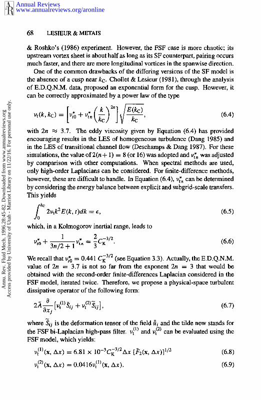
One of the common drawbacks of the differing versions of the SF model is the absence of a cusp near kc . Chollet & Lesieur (1981), through the analysis of E.D.Q.N.M. data, proposed an exponential form for the cusp. However, it can be correctly approximated by a power law of the type
with 2n x 3.7. The eddy viscosity given by Equation (6.4) has provided encouraging results in the LES of homogeneous turbulence (Dang 1985) and in the LES of transitional channel flow (Deschamps & Dang 1987). For these simulations, the value of 2(n + 1) = 8 (or 16) was adopted and u:n was adjusted by comparison with other computations. When spectral methods are used, only high-order Laplacians can be considered. For finite-difference methods, however, these are difficult to handle. In Equation (6.4), ut*, can be determined by considering the energy balance between explicit and subgrid-scale transfers. This yields
I" 2utk2E(k, r)dk = E ,
which, in a Kolmogorov inertial range, leads to
We recall that uTo = 0.441 CK3" (see Equation 3.3). Actually, the E.D.Q.N.M. value of 2n = 3.7 is not so far from the exponent 2n = 3 that would be obtained with the second-order finite-differences Laplacian considered in the FSF model, iterated twice. Therefore, we propose a physical-space turbulent dissipative operator of the following form:
where Z j j is the deformation tensor of the field ti and the tilde now stands for the FSF bi-Laplacian high-pass filter. u:') and ut(2) can be evaluated using the FSF model, which yields:
(6.8)
(6.9)
u;')(x, AX) = 6.81 x 10⁻³Ci3/2A~ [F~(x, u,(')(x, AX) = 0.0416~,( ' ) (~, AX).
Annual Reviewswww.annualreviews.org/aronline
Ann
u. R
ev. F
luid
Mec
h. 1
996.
28:4
5-82
. Dow
nloa
ded
from
ww
w.a
nnua
lrev
iew
s.or
g A
cces
s pr
ovid
ed b
y U
nive
rsity
of
Uta
h -
Mar
riot
Lib
rary
on
11/2
2/16
. For
per
sona
l use
onl
y.

LARGE-EDDY SIMULATIONS OF TURBULENCE 69
The constant A is defined by
G, (6.10) 4 3 5 - m A=--
5 m + l for m 5 3, where m is the slope of the spectrum E ( k ) at the cutoff; it is set equal to zero for m > 3. This constant accounts for the deviation from a Kolmogorov spectrum, as in Lamballais’ model described by Equation (3.7).
which yields m = a -+ 1 - S. For the FSF bi-Laplacian, a = 6 and If we let E ( k ) o( k‘k-m, one can easily show that &(r) 0: rm-‘-l - - r-’,
m. - 4 % - 2 A = - - 5 8 - S
(6.11)
We recall that S characterizes the asymptotic behavior of Fz(r) in the neigh- borhood of Ax. The condition m > 3 (where the eddy viscosity has to be set equal to zero) corresponds to 9 < 4. For a Kolmogorov spectrum, S = 16/3. This new “spectral-cusp FSF’ model should be tested in boundary-layer flows.
In the same spirit, one may mention a formulation of the turbulent dissipative operator, suggested by JH Ferziger (1995, private communication), that uses Smagorinsky’s model as a base model combined with a bi-Laplacian operator (n = 1). In this case, the constants are determined using the dynamic procedure presented in Section 8.
7. SCALE-SIMILARITY AND MIXED MODELS The eddy-viscosity closures assume a one-to-one correlation between the sub- grid-scale stress and the large-scale strain rate tensors. The analysis of fields obtained from DNS has, however, displayed very little correlation between the two tensors (see e.g. Clark et a1 1979, McMillan & Ferziger 1980). Liu et a1 (1994) recently confirmed this point in a much higher Reynolds number flow using the experimental data taken in the far field of a turbulent round jet. This lack of correlation between the two tensors has led Bardina et a1 (1980) to propose an alternative subgrid-scale model called the scale-similarity model. The model is based upon a double-filtering approach and on the idea that the important interactions between the resolved and unresolved scales involve the smallest eddies of the former and the largest eddies of the latter. Bardina et a1 suggest evaluating the subgrid tensor as
(7.1)
The analysis of DNS and experimental data (Bardina et a1 1980, Liu et a1 1994) have shown that the modeled subgrid-scale stress deduced from (7.1)
T. . - ;.E. -m I j - I J I j ’
Annual Reviewswww.annualreviews.org/aronline
Ann
u. R
ev. F
luid
Mec
h. 1
996.
28:4
5-82
. Dow
nloa
ded
from
ww
w.a
nnua
lrev
iew
s.or
g A
cces
s pr
ovid
ed b
y U
nive
rsity
of
Uta
h -
Mar
riot
Lib
rary
on
11/2
2/16
. For
per
sona
l use
onl
y.

70 LESIEUR & METAIS
exhibits a good correlation with the real (measured) stress. However, when implemented in LES calculations, the model hardly dissipates any energy. It is therefore necessary to combine it with an eddy-viscosity type model such as Smagorinsky’s model to produce the “mixed” model. Along the lines of the Bardina et a1 model, new formulations have been proposed to correct for this lack of dissipation. Goutorbe et a1 (1994) and Liu et a1 (1994) have proposed models with
1;:j = C,(B,rij - i i i j ) , (7.2)
where CL is a dimensionless coefficient. The models differ through an operator (notated by a tilde) that either corresponds to a spatial average (Goutorbe et a1 1994) or to a second filter of different width (Liu et al 1994). This concept of double filtering can be taken one step further, leading to the dynamic models presented in the next section.
8. DYNAMIC MODELS We noted that, for Kraichnan’s eddy viscosity, the parameters defining it could be computed from a LES with a cutoff kc, by defining a fictitious cutoff kb = kc/2, and explicitly calculating the transfers across k& (Lesieur & Rogallo 1989). This is the underlying philosophy of the dynamic model of Germano et a1 (1991, see also Germano 1992). Their method relies on a LES using a “base” subgrid-scale model such as Smagorinsky’s model, with a grid mesh Ax. The computed fields 7 are filtered by a “test filter” (notated by a tilde) of larger width aAx (for instance a = 2), to yield the field 7. If one applies the double filter to the Navier-Stokes equation (with constant density), the subgrid-scale tensor of the field that must be modeled is
Let us now consider the resolved turbulent stress corresponding to the test filter applied to the field ii:
The latter is equivalent to Leonard’s tensor associated with the test filter. Note that we use signs opposite to those of Germano et a1 (1991), again, because the terms become stresses when multiplied by p. It follows from these two definitions that
Annual Reviewswww.annualreviews.org/aronline
Ann
u. R
ev. F
luid
Mec
h. 1
996.
28:4
5-82
. Dow
nloa
ded
from
ww
w.a
nnua
lrev
iew
s.or
g A
cces
s pr
ovid
ed b
y U
nive
rsity
of
Uta
h -
Mar
riot
Lib
rary
on
11/2
2/16
. For
per
sona
l use
onl
y.
LARGE-EDDY SIMULATIONS OF TURBULENCE 7 1
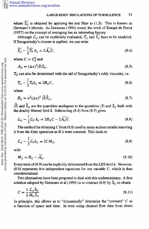
where is obtained by applying the test filter to (1.5). This is known as Germano’s identity. As Germano (1994) noted, the work of KampC de Feriet (1957) on the concept of averaging has an interesting h3tory.
Although Lij can be explicitely evaluated, ?;i and cj have to be modeled. If Smagorinsky’s closure is applied, we can write
where C = Ci and
Aij = ( A ~ ) ~ l S l S i j . (8.5)
zj can also be determined with the aid of Smagorinsky’s eddy viscosity, i.e.
- 131 and Si, are the quantities analogous to the quantities 131 and Si, built with the doubly filtered field f . Subtracting (8.4) from (8.5) gives
The method for obtaining C from (8.8) used by many authors entails removing it from the filter operation as if it were constant. This leads to
1 Lij - ~ L ~ ~ G i j = 2CMij , (8.9)
with - Mij = Bij - Ai,. (8.10)
Every term of (8.9) can be explicitly determined from the LES field fi. However, (8.9) represents five independent equations for one variable C, which is thus overdetermined.
Two alternatives have been proposed to deal with this undeterminacy. A first solution adopted by Germano et a1 (1991) is to contract (8.9) by Si j to obtain
(8.1 1)
In principle, this allows us to “dynamically” determine the “constant” C as a function of space and time. In tests using channel flow data from direct
Annual Reviewswww.annualreviews.org/aronline
Ann
u. R
ev. F
luid
Mec
h. 1
996.
28:4
5-82
. Dow
nloa
ded
from
ww
w.a
nnua
lrev
iew
s.or
g A
cces
s pr
ovid
ed b
y U
nive
rsity
of
Uta
h -
Mar
riot
Lib
rary
on
11/2
2/16
. For
per
sona
l use
onl
y.

72 LESIEUR & METAIS
numerical simulations, Germano et a1 (1991) have shown, however, that the denominator in (8.1 1) could locally vanish or become sufficiently small, thereby leading to computational instabilities. Lilly (1992) chose to determine the value of C that “best satisfies” the system (8.9) by minimizing the error using a least- squares approach, i.e.
(8.12)
This technique removes the local undeterminacy attached to the original formulation (8.1 l), and this form has become the most widely used (see e.g. Piomelli 1993, Sreedhar & Ragab 1994).
Unfortunately, analysis of DNS data (Lund et a1 1993) and of experimental data (Liu et a1 1994) revealed that the C field predicted by the models (8.11) or (8.12) varies strongly in space and contains a significant fraction of nega- tive values: Its variance may reach values as high as 10 times the square of its mean value! Therefore, the removal of the “constant” C from the filter operation is not a posteriori justified, and the model exhibits some mathemat- ical inconsistencies (see e.g. Ghosal et a1 1995 for a discussion on that point). The allowance of negative values of C is an advantage of the model because these values represent a sort of backscatter in physical space, which replaces the spectral k4 backscatter previously mentioned. However, very large negative values of the eddy viscosity is a destabilizing process in a numerical simulation, and a nonphysical growth of the resolved scale energy has often been observed (Lund et a1 1993). The cure often adopted to avoid excessively large values of C consists in averaging the numerators and denominators of (8.11) and (8.12) over space and/or time, thereby losing some of the conceptual advantages of the “dynamic” local formulation. However, averaging over direction of flow homogeneity has been a popular choice, and this has produced good results. For example, Germano et a1 (1991) and Piomelli (1993) used an average in planes parallel to the walls in their channel flow simulation. They showed that the dynamic model gives a zero subgrid-scale stress at the wall, where Lij vanishes, which is a great advantage with respect to the original Smagorinsky model; it also yields the proper asymptotic behavior near the wall. Compar- isons with DNS at R = 3300 (based upon the centerline velocity and the channel half-width) and with experiments at high Reynolds number are good, and encouraging results are obtained for transition. Notice that, in the channel center, Piomelli (1993) obtained CS x 0.06, a value slightly lower than the commonly used values in “classical” Smagorinsky’s formulation. Note also that the use of Smagorinsky’s model as a base for the dynamic procedure is not compulsory, and any of the models described in the present paper can be a candidate. As examples, Zang et a1 (1993) and K Shah & JH Ferziger (1995,
Annual Reviewswww.annualreviews.org/aronline
Ann
u. R
ev. F
luid
Mec
h. 1
996.
28:4
5-82
. Dow
nloa
ded
from
ww
w.a
nnua
lrev
iew
s.or
g A
cces
s pr
ovid
ed b
y U
nive
rsity
of
Uta
h -
Mar
riot
Lib
rary
on
11/2
2/16
. For
per
sona
l use
onl
y.

LARGE-EDDY SIMULATIONS OF TURBULENCE 73
personal communication; see below) have successfully utilized this procedure in the “mixed” model (cf previous section) [see also Goutorbe et a1 (1994), Ghosal et a1 (1995), and El-Hady & Zang (1995) for other models].
The drawback of the averaging procedure is that it restricts the model appli- cability to a simple flow geometry with at least one direction of homogeneity. An alternative formulation has been suggested by Meneveau et a1 (1994) in which the error associated with Germano’s identity is minimized along par- ticle trajectories rather than directions of statistical homogeneity. The model is shown to produce results equal or superior to those of spatially averaged versions of the dynamic model. However, two additional transport equations need to be solved, which somewhat increases the computational cost. In a work in progress, K Shah & JH Ferziger (1995, personal communication) use the “mixed” model with Smagorinsky’s eddy viscosity as a base model for the dynamic procedure. C is obtained through Equation (8.12). However, the two tensors Cij and Mi, in (8.12) are not directly evaluated with the LES field 17, but with the aid of aprefiltered field h, where the circumflex designates an additional filter of width 1.5Ax; the test-filter width is kept equal to 2Ax. The advantage of this extra filtering is to considerably curtail the variance of C , and therefore it precludes the necessity of spatial averaging. This model has been implemented by K Shah & JH Ferziger (1995, personal communication) in a finite-volume nu- merical code to simulate the three-dimensional (nonhomogeneous) flow around a cube mounted on the bottom wall of a channel at a Reynolds number of 3000 (based upon the upstream mean velocity and the cube height). The numeri- cal results have been compared with the laboratory experiment performed by Martinuzzi (1992) at Re = 40,000. Although the numerical and experimental Reynolds numbers are very different, a good agreement was found, outside the boundary-layer regions, for the mean velocity profiles measured at different streamwise locations. Furthermore, and in spite of the flow complexity, the temporally averaged streamlines near the bottom boundary layer obtained in the LES (Figure 10) exhibit features almost identical to those experimentally observed with oil film techniques. The separation distance upstream of the obstacle is different in both cases, due to Reynolds number effects.
The mathematical inconsistency attached with the extraction of C from the filtering operation in (8.8), as well as the limitations introduced by the spatial average in the direction of flow homogeneity, have recently been addressed by Ghosal et a1 (1995). They use a global variational approach to properly account for the spatial variation of the coefficient within the filter operation. Two mod- els are derived that allow a generalization of the dynamic procedure to flows that do not necessarily possess homogeneous directions. The constraint C 2 0 was imposed in the first model, in order to permit the derivation of an integral
Annual Reviewswww.annualreviews.org/aronline
Ann
u. R
ev. F
luid
Mec
h. 1
996.
28:4
5-82
. Dow
nloa
ded
from
ww
w.a
nnua
lrev
iew
s.or
g A
cces
s pr
ovid
ed b
y U
nive
rsity
of
Uta
h -
Mar
riot
Lib
rary
on
11/2
2/16
. For
per
sona
l use
onl
y.

74 LESIEUR & METAIS
equation for C. This model is referred to as the constrained dynamic localiza- tion model. However, this constraint forbids possible backscatter, which has motivated the development of a second model enforcing a budget for the inverse energy transfer through the inclusion of a transport equation for the subgrid- scale kinetic energy. This model is called the k-equation dynamic localization model. Note that the use of additional transport equations in LES was previ- ously adopted by several authors (see e.g. Deardorff 1973, Schumann 1975, and Grotzbach & Schumann 1979). Ghosal et a1 (1995) have tested their mod- els in forced isotropic turbulence and in the flow over a backward-facing step. Figure 11 shows the prediction of Kolmogorov’s k-5/3 and the Kolmogorov compensated spectra in forced isotropic turbulence obtained from the dynamic
6.00
5.00
4.00
3.00
2.00
1.00
1 .00 2.00 3.M) 4.00 5.00 6.00 7.00
Figure 10 LES of three-dimensional flow around a cube mounted on the bottom wall of a channel at a Reynolds number of 3000 (dynamic mixed model). Shown are temporally averaged streamlines near the bottom boundary layer. [Courtesy K Shah & JH Ferziger (1995, private communication).]
Annual Reviewswww.annualreviews.org/aronline
Ann
u. R
ev. F
luid
Mec
h. 1
996.
28:4
5-82
. Dow
nloa
ded
from
ww
w.a
nnua
lrev
iew
s.or
g A
cces
s pr
ovid
ed b
y U
nive
rsity
of
Uta
h -
Mar
riot
Lib
rary
on
11/2
2/16
. For
per
sona
l use
onl
y.
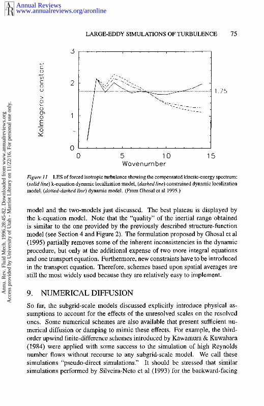
LARGE-EDDY SIMULATIONS OF TURBULENCE 75
+- C
1 .75
0 5 10 15 Wavenumber
Figure I I LES of forced isotropic turbulence showing the compensated kinetic-energy spectrum: (solid line) k-equation dynamic localization model, (dashed line) constrained dynamic localization model, (dotted-dashed line) dynamic model. (From Ghosal et al 1995.)
model and the two-models just discussed. The best plateau is displayed by the k-equation model. Note that the “quality” of the inertial range obtained is similar to the one provided by the previously described structure-function model (see Section 4 and Figure 2). The formulation proposed by Ghosal et a1 (1995) partially removes some of the inherent inconsistencies in the dynamic procedure, but only at the additional expense of two more integral equations and one transport equation. Furthermore, new constraints have to be introduced in the transport equation. Therefore, schemes based upon spatial averages are still the most widely used because they are relatively easy to implement.
9. NUMERICAL DIFFUSION So far, the subgrid-scale models discussed explicitly introduce physical as- sumptions to account for the effects of the unresolved scales on the resolved ones. Some numerical schemes are also available that present sufficient nu- merical diffusion or damping to mimic these effects. For example, the third- order upwind finite-difference schemes introduced by Kawamura & Kuwahara (1984) were applied with some success to the simulation of high Reynolds number flows without recourse to any subgrid-scale model. We call these simulations “pseudo-direct simulations.” It should be stressed that similar simulations performed by Silveira-Net0 et a1 (1993) for the backward-facing
Annual Reviewswww.annualreviews.org/aronline
Ann
u. R
ev. F
luid
Mec
h. 1
996.
28:4
5-82
. Dow
nloa
ded
from
ww
w.a
nnua
lrev
iew
s.or
g A
cces
s pr
ovid
ed b
y U
nive
rsity
of
Uta
h -
Mar
riot
Lib
rary
on
11/2
2/16
. For
per
sona
l use
onl
y.
76 LESIEUR & METAIS
step have displayed very bad agreement with the experiments. Boris et al(l992) showed that the Piecewise Parabolic Method (PPM) also has intrinsically the features of a dissipative subgrid-scale model. Porter et a1 (1994) used this nu- merical method to simulate a 3D, decaying supersonic turbulent flow at high Reynolds number. The development of a k-5/3 kinetic-energy spectrum was observed at large scales for the solenoidal part of the velocity field, and a new spectral behavior of shallower slope ( Z k - ' ) was found in the smaller scales. Note that when using these techniques one has to make sure that the numerical diffusion exactly meets the requirements of the subgrid-scales, and the results obtained with such numerical methods have to be checked very carefully.
10. CONCLUSIONS In this paper, we have tried to present the main recent trends of large-eddy sim- ulation techniques. Large-eddy simulations allow us to focus attention on the large scales while the scales unresolved by the grid mesh are modeled with some generalized eddy viscosity. When a passive scalar is convected by the flow, one also introduces an eddy diffusivity. The latter is generally taken to be propor- tional to the eddy viscosity through the assumption of a constant Prandtl number.
The most popular model for engineering application purposes when small- scale turbulence is three dimensional is certainly Smagorinsky 's model (1963), where the eddy viscosity is proportional to the square of the grid mesh Ax times the local strain rate. The constant arising in the model may be determined if one assumes that subgrid-scale turbulence is isotropic and follows a Kolmogorov k-'I3 inertial range, but this adjustment is questionable in transient situations or in the proximity of boundaries. This provides the motivation for dynamic models, where an attempt is made to evaluate the constant dynamically through a double filtering. Standard Smagorinsky's model gives interesting results (as far as coherent structures are concerned, for instance) in isotropic turbulence and in free-shear flows, but fails in the presence of a boundary, where the eddy viscosity due to the mean strain is too high to allow for the growth of viscous instabilities.
Another class of subgrid models may be introduced if one works in Fourier space. Kraichnan's (1976) spectral eddy viscosity, which expresses the action of modes > k c = rr/Ax upon the subgrid-modes k 5 k c , is proportional to [ E ( k ~ ) / k c ] ' / ~ , where E ( k c ) is the kinetic-energy spectrum at the cutoff. It is independant of k except in the neighborhood of k c , where it rises sharply in a cusp. From an energetic point of view, it takes into account all the in- teractions across k c , including the backscatter. This model gives very good results for mixing layers; in particular, it provides information about possible longitudinal stretching or dislocations of the vortex field according to the types
Annual Reviewswww.annualreviews.org/aronline
Ann
u. R
ev. F
luid
Mec
h. 1
996.
28:4
5-82
. Dow
nloa
ded
from
ww
w.a
nnua
lrev
iew
s.or
g A
cces
s pr
ovid
ed b
y U
nive
rsity
of
Uta
h -
Mar
riot
Lib
rary
on
11/2
2/16
. For
per
sona
l use
onl
y.

LARGE-EDDY SIMULATIONS OF TURBULENCE 77
of perturbations forcing the flow. It also aptly describes the decay of three- dimensional isotropic turbulence at infinite Reynolds number for flows with an initial spectrum sharply peaking at kl . In a preliminary stage, kinetic energy cascades up to kc, while being conserved. Afterwards, the spectrum decays self-similarly with a k-2 slope close to the cutoff. Meanwhile, a k4 backscatter is produced for k c k l . A finite-time singularity for the enstrophy is thus obtained, if the latter is determined by extrapolation of the cutoff spectrum at the subgrid scales.
The structure-function model (MCtais & Lesieur 1992) is designed to mimic the action of spectral eddy viscosity (without a cusp) in physical space. A local kinetic-energy spectrum at the cutoff is introduced, which is determined in terms of the local second-order velocity structure function. The latter is evaluated by a local averaging on the six (in a volume) or four (in a plane) closest points on the grid. The SF model yields a good Kolmogorov energy spectrum for isotropic turbulence (better than Smagorinsky’s, which has a steeper spectrum), as well as hints of Batchelor’s k-7/3 quasi-normal law for the pressure spectrum, with the right constant. The SF model also preserves the pressure large-scale inter- mittency, with a pressure PDF that is exponential in the lows and Gaussian in the highs. The SF model has been applied satisfactorily to wakes (temporal and spatial) and to a backstep flow, where it improves upon Smagorinsky’s results. We have also discussed, in the limit of a vanishing mesh, the relationships between both models. In the four-point formulation (averages carried out in planes parallel to the wall), the SF model allows one to continue past the tran- sition of the second mode in a temporal boundary layer on an adiabatic plate at Mach 4.5. However, at low Mach number, the SF model is still too dissipative.
We also described a selective version of the SF model, where the eddy viscos- ity is weighted in such a way that it is active only in regions of space where the flow presents a certain degree of three dimensionality. The 3D criterion consists of looking at the relative orientation of the vorticity vector and the average of the vorticity vectors of the closest points, by comparison with the most probable values obtained in DNS of isotropic turbulence. This SSF model was shown to behave very well in a stably stratified backstep flow, where stratification is a strong two-dimensionalization factor, and in a supersonic compression ramp at Mach 2.5, where longitudinal Gortler-type vortices are produced that severely affect the heating at the boundary. Another way of improving the performance of the SF model, for transition on a flat plate, is to apply a high-pass filter to the flow and to compute the local spectrum E(kc) in terms of the filtered field structure-function. This allows the eddy viscosity to rid the flow of large-scale fluctuations and shears. Such a filtered structure-function model (FSF) allows one to simulate at a not-too-excessive cost the whole transition to turbulence
Annual Reviewswww.annualreviews.org/aronline
Ann
u. R
ev. F
luid
Mec
h. 1
996.
28:4
5-82
. Dow
nloa
ded
from
ww
w.a
nnua
lrev
iew
s.or
g A
cces
s pr
ovid
ed b
y U
nive
rsity
of
Uta
h -
Mar
riot
Lib
rary
on
11/2
2/16
. For
per
sona
l use
onl
y.
78 LESIEUR & METAIS
in a weakly compressible, spatially growing boundary layer. The model is also very efficient for incompressible spatial mixing layers.
In scale-similarity models (Bardina et a1 1980), the subgrid-scale stresses are evaluated by a further filtering on a larger mesh of the field ii, as if the latter was the actual field u. More recently, Germano et a1 (1991) introduced the dynamic model, where a double filtering allows one to recompute Cg, the constant arising in Smagorinsky’s model, as a function of space and time. Since the latter is determined with the aid of a tensorial equation, problems arise due to either local undeterminacies (in Germano et al’s 1991 formulation) or to excessive backscatter (C: < 0) in Lilly’s (1992) formulation; these lead rapidly to a divergence of the simulation. This is the reason one must average Cg in directions of homogeneity. Although this averaging is somewhat inconsistent with the original dynamic modeling philosophy, it gives good results for channel flows (where averages are performed in planes parallel to the boundaries) or for backstep flows (with an averaging in the spanwise direction). More recently, new dynamic models have been developed by Ghosal et a1 (1995), where either backscatter in physical space is forbidden or controlled by an evolution equation following ii of the subgrid kinetic energy.
We discussed other models that take into account the cusp arising in Kraich- nan’s spectral eddy viscosity, through iterated Laplacians. Finally, we also briefly discussed pseudo-direct simulations in which numerical diffusion is supposed to take care of subgrid transfers.
Large-eddy simulations are undergoing a blooming development, based both on the new subgrid modeling methods presented in this paper and on the tremendous progress in scientific computing. Confined in the past to very sim- ple configurations such as isotropic turbulence or periodic flows, geometries are progressively evolving to spatially growing shear or separated flows, pipe flows, riblet-mounted channels, etc. In these cases, LES, allied with DNS, are now able to provide both deterministic (in terms of coherent-vortex dynamics for instance) and statistical predictions. This stage is very important, particularly for assessing and possibly improving the one-point closure models. There is no doubt that the complexity of problems tackled by LES techniques is going to increase, and this will have a decisive impact on industrial modeling and control.
ACKNOWLEDGMENTS
We are indebted to P Bartello, P Comte, E David, F Ducros, B Fallon, JH Ferziger, MA Gonze, A Silveira-Neto, and J Silvestrini for useful discussions and for contributions to the work presented here.
We thank also CEA, CNES, CNRS, Dassault, DRET, INPG, and UJF for their support.
Annual Reviewswww.annualreviews.org/aronline
Ann
u. R
ev. F
luid
Mec
h. 1
996.
28:4
5-82
. Dow
nloa
ded
from
ww
w.a
nnua
lrev
iew
s.or
g A
cces
s pr
ovid
ed b
y U
nive
rsity
of
Uta
h -
Mar
riot
Lib
rary
on
11/2
2/16
. For
per
sona
l use
onl
y.

LARGE-EDDY SIMULATIONS OF TURBULENCE 79
Any Annual Review chapter, as well as any article cited in an Annual Review chapter, may be purchased from the Annual Reviews Preprints and Reprints service.
1-800-347-8007; 415-259-5017; email: [email protected]
Literature Cited
Adams EW, Johnston JP, Eaton JK. 1984. Exper- iments on the structure of turbulent reacting flows. Stanford Univ. Rep. MD-43j
Andre JC, Lesieur M. 1977. Influence of helic- ity on high Reynolds number isotropic turbu- lence. J. Fluid Mech. 81:187-207
Amal M, Friedrich R. 1992. Large-eddy sim- ulation of a turbulent flow with separation. In Turbulent Shear Flows Vlll, ed. U Schu- mann, F Durst, BE Launder, FW Schmidt, JH Whitelaw, p. 169. Berlin: Springer-Verlag
Bardina J, Ferziger JH, Reynolds WC. 1980. Im- proved subgrid model for large-eddy simula- tion. A I M Pap. 80-1357
Bartello P, MBtais 0, Lesieur M. 1994. Coher- ent structures in rotating three-dimensional turbulence. J. Fluid Mech. 273:l-29
Basdevant C, Sadourny R. 1983. Moddlisation des Bchelles virtuelles dans la simulation numBrique des Bcoulements bidimensionnels , J. Mic. Theor: Appl., NumBro Spec., pp. 243- 69
Batchelor GK. 1953. The Theory of Homoge- neous Turbulence. Cambridge: Cambridge Univ. Press. 197 pp.
Batchelor GK, Canuto C, Chasnov J. 1992. Ho- mogeneous buoyancy-generated turbulence. J. Fluid Mech. 235:349-78
Bernal LP, Roshko A. 1986. Streamwise vortex structure in plane mixing layer. J. Fluid Mech.
Boris JP, Grinstein FF, Oran ES, Kolbe RL. 1992. New insights into large-eddy simula- tion. Fluid Dyn. Res. 10:199-228
Breuer M, Rodi W. 1994. Large-eddy simulation of turbulent flow through straight and curved ducts. ERCOFTAC Bull. 22:26-29
Cadot 0, Douady S, Couder Y. 1995. Character- ization of low-pressure filaments in a three- dimensional turbulent shear flow. Phys. Flu- ids 7(3):630-46
Cain AB. 1981. Three-dimensional simulation oj'transition and early turbulence in a time- developing mixing laye,: PhD thesis. Stanford Univ.
Cambon C, Benoit JP, Shao L, Jacquin L. 1994. Stability analysis and large-eddy simulation of rotating turbulence with organized eddies. J. Fluid Mech. 278:175-200
Champagne FH, Friehe CA, LaRue JC, Wyn- gaard JC. 1977. Flux measurements, flux es- timation techniques and fine-scale turbulence
170:499-525
measurements in the unstable surface layer over land. J. Atmos. Sci. 34:515-30
Chandrsuda C, Mehta RD, Weir AD, Bradshaw P. 1978. Effect of free-stream turbulence on large structure in turbulent mixing layers. J. Fluid Mech. 85:693-704
Chollet JP, Lesieur M. 1981. Parameterization of small scales of three-dimensional isotropic turbulence utilizing spectral closures. J. At- mos. Sci. 38:2747-57
Clark RA, Ferziger JH, Reynolds WC. 1979. Evaluation of subgrid-scale models using an accurately simulated turbulent flow. J. Fluid Mech. 91:l-16
Comte P. 1994. Structure-function based mod- els for compressible transitional shear flows.
Comte P, Lesieur M, Lamballais E. 1992. Large and small-scale stirring of vorticity and a pas- sive scalar in a 3D temporal mixing layer. Phys. Fluids A 4(12):2761-78
Corcos GM, Lin SJ. 1984. The mixinglayer: de- terministic models of a turbulent flow. Part 2. The origin of the three-dimensional motion. J. Fluid Mech. 139:67-95
Dang KT. 1985. Evaluation of simple subgrid- scale models for the numerical simulation of homogeneous turbulence. AIAA J. 23(2):221- 27
David E. 1993. Modilisation des icoulements compressibles et hypersoniques: une ap- proche instationnaire. PhD thesis. Natl. Poly- tech. Inst., Grenoble
DeardorffJW. 1970. A numerical study of three- dimensional turbulent channel flow at large Reynolds number. J. Fluid Mech. 41:453-80
Deardorff JW. 1973. The use of subgrid trans- port equations in a three-dimensional model of atmospheric turbulence. J. Fluids Eng.
Deschamps V, Dang KT. 1987. Evaluation of subgrid-scale models for large-eddy simula- tion of transitional channel flows. In Proc. of Sixth Symp. on Turbulent Shear Flows, pp. 20-1- 1,20- 1-7. Toulouse
Domaradzki JA, Metcalfe RW, Rogallo RS, Ri- ley JJ. 1987. Analysis of subgrid-scale eddy viscosity with the use of the results from di- rect numerical simulations. Phys. Rev. Lett.
Ducros F. 1995. Simulations numiriques di- rectes et des grandes echelles de couches lim-
ERCOFTAC Bull. 22:9-14
95 :429-38
58:547-50
Annual Reviewswww.annualreviews.org/aronline
Ann
u. R
ev. F
luid
Mec
h. 1
996.
28:4
5-82
. Dow
nloa
ded
from
ww
w.a
nnua
lrev
iew
s.or
g A
cces
s pr
ovid
ed b
y U
nive
rsity
of
Uta
h -
Mar
riot
Lib
rary
on
11/2
2/16
. For
per
sona
l use
onl
y.

80 LESIEUR & METAIS
ites compressibles. PhD thesis. Natl. Poly- tech. Inst., Grenoble
Ducros F, Comte P, Lesieur M. 1993. Ropes and lambda-vortices in direct and large-eddy simulations of a high Mach number bound- ary layer over a flat plate. In Turbulent Shear Flows IX, Kyoto, August 1993. To appear in the selected proc. Berlin: Springer-Verlag
Eaton JK, Johnston JP. 1980. Turbulent flow reattachment: an experimental study of the flow and structure behind a backward-facing step. Stanford Univ. Rep. MD-39
El-Hady NM, Zang TA. 1995. Large-eddy sim- ulation of nonlinear evolution and breakdown to turbulence in high-speed boundary layers. Theoret. Comput. Fluid. Dyn. 7:217-40
Fallon B. 1994. Simulations des g r a d e s ichelles d'icoulements turbulents .strat$& en densiti. PhD thesis. Natl. Polytech. Inst., Grenoble
Fauve S, Laroche C, Castaing B. 1993. Pres- sure fluctuations in swirling turbulent flows. J. Phys II (France) 3:271-78
Fouillet Y. 1991. Simulation numirique de tour- billons cohirents dans les e'ccoulements turbu- lents libres compressibles. PhD thesis. Natl. Polytech. Inst., Grenoble
Friedrich R, Nieuwstadt F. 1994. LES of pipe
Gathmann RJ, Si-Ameur M, Mathey F. 1993. Numerical simulation of three-dimensional natural transition in the compressible con- fined shear layer. Phys. FluidsA 5(11):2946- 68
Germano M. 1992. Turbulence, the filtering ap- proach. J. Fluid Mech. 238:325-36
Germano M. 1994. Dynamic models. ERCOF-
Germano M, Piomelli U, Moin P, Cabot W. 1991. A dynamic subgrid-scale eddy- viscosity model. Phys. Fluids A 3(7):1760- 65
Ghosal S, Lund TS, Moin P, Akselvoll K. 1995. A dynamic localization model for large-eddy simulation of turbulent flows. J. Fluid Mech.
Gonze MA. 1993. Simulation nume'rique des sil- luges en transition d la turbulence. PhD the- sis. Natl. Polytech. Inst., Grenoble
Goutorbe T, Laurence D, Maupu V. 1994. A pri- ori test of a subgrid scale stress tensor model including anisotropy and backscatter effects. In Direct and Large-Eddy Simulation I, ed. PR Voke, L Kleiser, JP Chollet, pp. 121-31. Dordrecht: Kluwer 434 pp.
Grotzbach G, Schumann U. 1979. Direct nu- merical simulation of turbulent velocity-, pressure-, and temperature-fields in channel flows. In Turbulenr Shear Flowsl, ed. FDurst, BE Launder, FW Schmidt, JH Whitelaw, pp.
flows. ERCOFTAC Bull. 22: 19-25
TAC Bull. 22:15-18
286:229-55
370-85. Berlin: Springer-Verlag Herring JR. 1979. Subgrid scale modeling-
An introduction and overview. In Turbulent Shear Flows I , ed. F Durst, BE Launder, FW Schmidt, JH Whitelaw, pp. 347-52. Berlin: Springer-Verlag
Herring JR, Schertzer D, Lesieur M, Newman GR, Chollet JP, Larchev2que M. 1982. A comparative assessment of spectral closures as applied to passive scalar diffusion. J. Fluid Mech. 124:411-37
Ho CM, Huerre P. 1984. Perturbed free shear layers. Annu. Rev. Fluid Mech. 16:365424
Huang LS, Ho CM. 1990. Small-scale transi- tion in a plane mixing layer. J. Fluid Mech.
Jimenez J, Wray AA, Saffman PG, Rogallo R. 1993. The structure of intense vorticity in isotropic turbulence. J. Fluid Mech. 255:65- 90
Kaltenbach HJ, Schumann U, Gerz T. 1994. Large-eddy simulation of turbulent diffusion in stably-stratified flow. J. Fluid Mech. 280: 1-40
Kampt5 de Feriet J. 1957. La notion de moyenne dans la thkorie de la turbulence. Rend. Sem. Mat. Fix Milano 27: 167-207
Kawamura T, Kuwahara K. 1984. Computation of high Reynolds number Flow around a cir- cular cylinder with surface roughness. AIAA Pap, 84-0340
Kim J, Moin P, Moser R. 1987. Turbulence statistics in fully developed channel flow at low Reynolds number. J. Fluid Mech. 177:133-66
Kleiser L, Zang TA. 1991. Numerical simula- tion of transition in wall-bounded shear flows. Annu. Rev. Fluid Mech. 23:495-537
Kline SJ, Reynolds WC, Schraub FA, Run- stadler PW, 1967. The structure of turbulent- boundary layers. J. Fluid Mech. 30:741-73
Kolmogorov AN. 1941. The local structure of turbulence in incompressible viscous fluid for very large Reynolds numbers. Dokl. Akad. NaukSSSR 30:301-5
Kraichnan RH. 1976. Eddy viscosity in two and three dimensions. J. Atmos. Sei. 33:1521-36
Larcheveque M, Chollet JP, Herring JR, Lesieur M, Newman GR, Schertzer D. 1980. Two- point closure applied to a passive scalar in decaying isotropic turbulence. In Turbulent Shear Flows 11, ed. LJS Bradbury, F Durst, BE Launder, FW Schmidt, JH Whitelaw, pp. 50-65. Berlin: Springer-Verlag
k i t h CE. 1990. Stochastic backscatter in a
2 10:475-500
subgrid-scale model: plane shear mixing layer. Phys. Fluids A 2(3):297-300
Leith CE, Kraichnan RH. 1972. Predictability of turbulent flows. J. Atmos. Sei. 29:1041-58
Lele SK. 1992. Compact finite difference
Annual Reviewswww.annualreviews.org/aronline
Ann
u. R
ev. F
luid
Mec
h. 1
996.
28:4
5-82
. Dow
nloa
ded
from
ww
w.a
nnua
lrev
iew
s.or
g A
cces
s pr
ovid
ed b
y U
nive
rsity
of
Uta
h -
Mar
riot
Lib
rary
on
11/2
2/16
. For
per
sona
l use
onl
y.
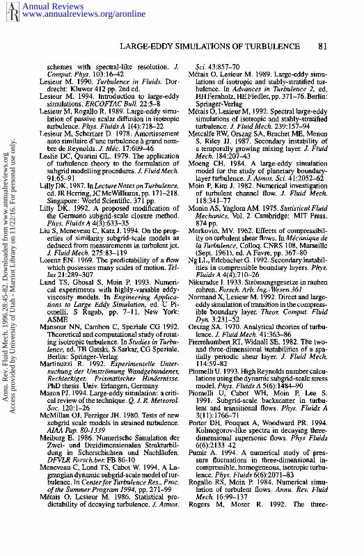
LARGE-EDDY SIMULATIONS OF TURBULENCE 8 1
schemes with spectral-like resolution. J. Comput. Phys. 103:16-42
Lesieur M. 1990. Turbulence in Fluids. Dor- drecht: Kluwer 412 pp. 2nd ed.
Lesieur M. 1994. Introduction to large-eddy simulations. ERCOFTAC Bull. 225-8
Lesieur M, Rogallo R. 1989. Large-eddy simu- lation of passive scalar diffusion in isotropic turbulence. Phys. Fluids A 1(4):718-22
Lesieur M, Schertzer D. 1978. Amortissement auto similaire d’une turbulence ?i grand nom- bre de Reynolds. J. M k . 17:60946
Leslie DC, Quarini GL. 1979. The application of turbulence theory to the formulation of subgrid modelling procedures. J. FluidMech. 9 1 :65-9 1
Lilly DK. 1987. In Lecture Notes on Turbulence, ed. JRHerring, JCMcWilliams, pp. 171-218. Singapore: World Scientific. 371 pp.
Lilly DK. 1992. A proposed modification of the German0 subgrid-scale closure method. Phys. Fluids A 4(3):633-35
Liu S , Meneveau C, Katz J. 1994. On the prop- erties of similarity subgrid-scale models as deduced from measurements in turbulent jet. J. Fluid Mech. 275:83-119
Lorenz EN. 1969. The predictability of a flow which possesses many scales of motion. Tel-
Lund TS, Ghosal S, Moin P. 1993. Numeri- cal experiments with highly-variable eddy- viscosity models. In Engineering Applicu- tions to Large Eddy Simulation, ed. U Pi- omelli, S Ragab, pp. 7-11. New York: ASME
Mansour NN, Cambon C, Speziale CG 1992. Theoretical and computational study of rotat- ing isotropic turbulence. In Studies in Turbu- lence, ed. TB Gatski, S Sarkar, CG Speziale. Berlin: Springer-Verlag
Martinuzzi R. 1992. Experimentelle Unter- suchung der Umstriimung Wandgebundenec Rechteckigec Prismatischer Hindernisse. PhD thesis. Univ. Erlangen, Germany
Mason PJ. 1994. Large-eddy simulation: acriti- cal review of the technique. Q. J. R. Meteorol.
McMillan OJ, Ferziger JH. 1980. Tests of new subgrid scale models in strained turbulence. AIAA Pap. 80-1339
Meiburg E. 1986. Numerische Simulation der Zwei- und Dreidimensionalen Strukturbil- dung in Scherschichten und Nachlaufen. DFVLR Forsch.ber FB 86-10
Meneveau C, Lund TS, Cabot W. 1994. A La- grangian dynamic subgrid-scale model of tur- bulence. In Centerfor Turbulence Res., Pmc. of the Summer Program 1994, pp. 271-99
MBtais 0, Lesieur M. 1986. Statistical pre- dictability of decaying turbulence. J. Atmos.
l ~ . ? 21 1289-307
SOC. 12O:l-26
Sci. 43:857-70 MBtais 0, Lesieur M. 1989. Large-eddy simu-
lations of isotropic and stably-stratified tur- bulence. In Advances in Turbulence 2, ed HHFernholz, HEFiedler, pp. 371-76. Berlin Springer-Verlag
MBtais 0, Lesieur M, 1992. Spectral large-eddy simulations of isotropic and stably-stratified turbulence. J. Fluid Mech. 239: 157-94
Metcalfe RW, Orszag SA, Brachet ME, Menon S, Riley JJ. 1987. Secondary instability of a temporally growing mixing layer. J. Fluid Mech. 184:20743
Moeng CH. 1984. A large-eddy simulation model for the study of planetary boundary- layer turbulence. J. Atmos. Sci. 4 1 :2052-62
Moin P, Kim J. 1982. Numerical investigation of turbulent channel flow. J. Fluid Mech.
Monin AS, Yaglom AM. 1975. Stutistical Fluid Mechanics, Vol. 2. Cambridge: MIT Press. 874 pp.
Morkovin, MV. 1962. Effects of compressibil- ity on turbulent shear flows. In Micanique de la Turbulence, Colloq. CNRS 108, Marseille (Sept. 1961), ed. A Favre, pp. 367-80
Ng LL, Erlebacher G. 1992. Secondary instabil- ities in compressible boundary layers. Phys. Fluids A 4(4):710-26
Nikuradse J. 1933. Stromungsgesetze in rauhen rohren. Forsch. Arb. 1ng.-Wesen 361
Normand X , Lesieur M. 1992. Direct and large- eddy simulation of transition in the compress- ible boundary layer. Theox Comput. Fluid Dyn. 3:231-52
Orszag SA. 1970. Analytical theories of turbu- lence. J. Fluid Mech. 41:363-86
Pierrehumbert RT, Widnall SE. and three-dimensional instab tially periodic shear layer. J. Fluid Mech.
Piomelli U. 1993. High Reynolds numbercalcu- lations using the dynamic subgrid-scale stress model. Phys. Fluids A 5(6):1484-90
Piomelli U, Cabot WH, Moin P, Lee S. 1991. Subgrid-scale backscatter in turbu- lent and transitional flows. Phys. F1uid.r A 3( 1 1): 1766-7 1
Porter DH, Pouquet A, Woodward PR. 1994. Kolmogorov-like spectra in decaying three- dimensional supersonic flows. Phys Fluids 6(6):213342
Pumir A. 1994. A numerical study of pres- sure fluctuations in three-dimensional in- compressible, homogeneous, isotropic turbu- lence. Phys. Fluids 6(6):2071-83
Rogallo RS, Moin P. 1984. Numerical simu- lation of turbulent flows. Annu. Rev. Fluid Mech. 16:99-137
Rogers M, Moser R. 1992. The three-
118:341-77
11459-82
Annual Reviewswww.annualreviews.org/aronline
Ann
u. R
ev. F
luid
Mec
h. 1
996.
28:4
5-82
. Dow
nloa
ded
from
ww
w.a
nnua
lrev
iew
s.or
g A
cces
s pr
ovid
ed b
y U
nive
rsity
of
Uta
h -
Mar
riot
Lib
rary
on
11/2
2/16
. For
per
sona
l use
onl
y.

82 LESIEUR & METAIS
dimensional evolution of a plane mixing layer: the Kelvin-Helmholtz roll up. J. Fluid Mech. 243:183-226
Sandham ND, Reynolds WC. 1991. Three- dimensional simulations of large eddies in the compressible mixing layer. J.-Fluid Mech.
Schumann U. 1975. Subgrid-scale model for fi- 224: 133-58
nite difference simulations of turbulent flows in plane channels and annuli. J. Compuf. Phys. 18:37&404
Scotti A, Meneveau C, Lilly DK. 1993. Gen- eralized Smagorinsky model for anisotropic grids. Phys. Fluids A 5(9):230&8
Siggia ED. 1981. Numerical study of small- scale intermittency in three-dimensional tur- bulence. J. Fluid Mech. 107:375-406
Silveira-Net0 A, Grand D, MBtais 0, Lesieur M. 1993. A numerical investigation of the coher- ent vortices in turbulence behind a backward- facing step. J. Fluid Mech. 256:l-25
Smagorinsky J. 1963. General circulation ex- periments with the primitive equations. Mon. Weather Rev. 91(3):99-164
Spalart PR. 1988. Direct simulation of a turbu- lentboundary layerup to Re = 1410. J. Fluid Mech. 187:61-98
Sreedhar M, Ragab S. 1994. Large-eddy simula- tion of longitudinal stationary vortices. Phys. Fluid 6(7):2501-14
Staquet S. 1991. Influenceofashearonastably- stratified flow. In Turbulence and Coherenf Sfrucfures, ed. 0 MBtais, MLesieur, pp. 469- 87. Dordrecht: Kluwer. 620 pp.
Unger F, Friedrich R. 1994. Large-eddy simula- tion of fully-developed turbulent pipe flow. In Flow Simulation of High-Peflormance Com- pufersl, ed. EH Hirschel, NNFM 38:201-16. Braunschweig: Vieweg-Verlag
Vincent A, Meneguzzi M. 1994. The dynamics of vorticity tubes in homogeneous turbulence. J. Fluid Mech. 258:245-54
Yakhot V, Orszag S. 1986. Renormalization Group (RNG) methods for turbulence clo- sure. J. Sci. Comput. 1:3-52
Yang Z , Voke PR. 1993. Large-eddy simula- tion studies of bypass transition. In Engi- neering Turbulence Modelling and Measure- ments, ed. W Rodi, F Martelli, pp. 603-1 1. Dordrecht: Elsevier
Zang Y, Street RL, Koseff JR. 1993. A dynamic mixed subgrid scale model and its application to turbulent recirculating flows. Phys. Fluids 5( 12x3 186-96
Annual Reviewswww.annualreviews.org/aronline
Ann
u. R
ev. F
luid
Mec
h. 1
996.
28:4
5-82
. Dow
nloa
ded
from
ww
w.a
nnua
lrev
iew
s.or
g A
cces
s pr
ovid
ed b
y U
nive
rsity
of
Uta
h -
Mar
riot
Lib
rary
on
11/2
2/16
. For
per
sona
l use
onl
y.