newsletter - acg.uwa.edu.au · required to initiate caving is able to be achieved and in fact well...

Australian Centre for Geomechanics | December 2013 Newsletter 1Continued page 2

A u s t r a l i a n C e n t r e f o r G e o m e c h a n i c s | V o l u m e N o . 4 7 | A u g u s t 2 0 1 8

IN THIS VOLUME:

1 Cave mining: challenges and future

5 mXrap: towards an integrated geotechnical model

7 Current mine waste disposal issues in South Africa and the status of paste and thickened tailings

9 Characterising the performance potential of polymer-treated tailings

12 Mining geomechanical risk - should we be doing better?

13 A new dynamic test facility for support tendons

16 The crack growth mechanicsm in biaxial compression - what happens on a face or sidewall of a drive?

19 Quantitative evaluation of economic risk for pit slope design

28 ACG event schedule

Cave mining: challenges and futureby Jarek Jakubec, SRK Consulting (Canada) Inc., Canada

Newsletter

IntroductionThere are over 50 cave mining

projects in various stages of studies and development around the world. Despite the fact that the cave mining method is more than 100 years old, it is only within the past 20 years that this mass mining method has spread from initial cave mining centres to six continents. There are currently approximately 17 cave mining operations in 11 countries.

The interest in cave mining is being fuelled by the depletion of near surface orebodies suitable for open pit operations, relatively high production rates and low operating cost. Also, a number of open pits have a continuation of the orebody below their economic depth, and further exploitation of often large low-grade resources at depth would not support a more expensive mining method. In recent years, besides the economics of high strip ratio, the environmental concern also plays an important role when comparing open pit mass mining and caving. Cave mines can have a significantly smaller footprint than a comparable open pit, since waste mined is only limited to underground

infrastructure development. In the case of deep large open pits, the footprint of the mining operation, including waste dumps, could be in the order of magnitude larger than for cave mining of the same orebody. This could be an even more significant constraint if the waste rock contains acid generating lithologies.

Cave mining principles and economics

Traditionally, caving methods were utilised for ore deposits that have well fractured rock mass that is not overly strong. The key importance is that the hydraulic radius (area over perimeter) required to initiate caving is able to be achieved and in fact well exceeded. In simple terms, cave mining was a method based on the principle of undercutting rock and then naturally letting it cave. However, this mining method has been extended to very strong rocks which would not easily cave or would not be suitable for caving due to very coarse fragmentation. To mitigate this problem, preconditioning techniques have been developed to generate more fractures and reduce the

4TH INTERNATIONAL

SYMPOSIUM ON

BLOCK AND

SUBLEVELCAVING

15–17 OCTOBER 2018

VANCOUVER, CANADA

Earlybird closes 3 Sept 2018

www.caving2018.com

Access development of Chuquicamata Mine (courtesy of Codelco)

UNDERGROUND

Australian Centre for Geomechanics | August 2018 Newsletter2

fragments to a manageable size. This is achieved by hydraulic fracturing and, in some cases, in combination with confined blasting. This technique, after rigorous testing, moved out of the domain of experimental mining to the mainstream design. Although some discussion is needed about the potential impact on in situ stress that is required for cave mining, several cave mines are in operation with preconditioned rock masses and several others are being developed. The most extensive work undertaken is at Cadia East mine and Northparkes Mines in Australia, and Andina and El Teniente in Chile.

Caving methods can be used with any type of commodity since it is the geological and geotechnical context that is important. There are many parameters to consider but typically the orebody needs to be at least 100 m thick for cave mining to be economical. In the past, typical caving heights were 150-250 m. Most of the designs which are on the drawing board today have caving lifts in excess of 350 m. Although higher lifts generally result in better NPV, they also have higher business risks of resource sterilisation, dilution, stability of the drawpoints, and extraction level in general.

By contrast, orebodies with relatively small horizontal footprints can also be mined economically if they have sufficient height and metal content to justify the capital expenditure. Good examples are Northparkes Mines in Australia, and the diamond mines in South Africa and Canada.

Mechanised cave mining includes

several variations of the method, including block, panel, incline and front caving. Most of the current mines and projects utilise either block or panel caving but after several years, Ekati Diamond Mine, Canada successfully introduced an incline cave at their Koala Mine.

Cave mining differs significantly from other typically more selective underground mining methods in a number of areas. Because cave mining is a bottom up method that relies on first establishing a large fixed infrastructure underground that will provide a very long-term production

platform, the initial capital costs are typically very high.

To offset the impact of the large capital expenditure on project value, a consequent high rate of production and an increased tonnage per drawpoint is required. In this day and age, several cave operations are running at upwards of 50,000 tpd and newer operations are being constructed for nameplate capacities of 100,000 tpd and more.

Chuquicamata and New Mining Levels at the El Teniente project in Chile; Oyu Tolgoi projects, Mongolia; Grasberg caving complex, Indonesia; and the Resolution Copper project in Arizona all fall into the supercaves category. It has to be stressed that there are no examples where tonnage over 100,000 tpd was achieved on a sustained basis from single cave footprint, although El Teniente produced higher tonnage from concurrently mining several caves.

In terms of logistics, once a cave mine is in production, the execution is relatively straightforward. The production footprint remains fixed and mining consumables typically revolve around secondary breaking with campaign maintenance within the production drives. The most significant logistics support is required for mobile equipment and fixed plant maintenance which are normally supported by large underground maintenance facilities. It is important that strict draw control is maintained and the extraction level is not experiencing excess

There are over 50 cave mining projects in various stages of studies and development around the world

Subsidence crater at Koala Diamond Mine (courtesy of Dominion Diamond Corporation)

© Copyright 2018. Australian Centre for Geomechanics (ACG), The University of Western Australia (UWA). All rights reserved. No part of this newsletter may be reproduced, stored or transmitted in any form without the prior written permission of the Australian Centre for Geomechanics, The University of Western Australia.

The information contained in this newsletter is for general educational and informative purposes only. Except to the extent required by law, UWA and the ACG make no representations or warranties express or implied as to the accuracy, reliability or completeness of the information contained therein. To the extent permitted by law, UWA and the ACG exclude all liability for loss or damage of any kind at all (including indirect or consequential loss or damage) arising from the information in this newsletter or use of such information. You acknowledge that the information provided in this newsletter is to assist you with undertaking your own enquiries and analyses and that you should seek independent professional advice before acting in reliance on the information contained therein.

The views expressed in this newsletter are those of the authors and may not reflect those of the Australian Centre for Geomechanics.

UNDERGROUND

Australian Centre for Geomechanics | August 2018 Newsletter 3

damage requiring repairs. Mudrushes and fines ingress can severely disrupt cave mining production.

Technical challenges of cave miningAs the number of cave mining projects

increases, there are also heightened expectations for high production rates and caving lifts, and greater depths to be achieved. The analysis of the cave mine performance is far from satisfactory. In the past two decades, at least 12 cave footprints were put into production and all experienced some level of unforeseen difficulty related to ground conditions, fragmentation, mining-induced seismicity, mudrushes, and underestimating ground support, or simply breaking basic cave mining rules, specifically in the area of undercutting and draw management.

On a positive note, in hindsight, most of the challenges could have been prevented with better upfront knowledge, correct design or draw disciplines.

The other disadvantage of cave mining is the long lead time. It typically takes 7 to 10 years, or longer, from initial studies to production and the site may underestimate the logistics and skillset required for cave mining development and operation.

Because the cave mine has to be fully developed before all design parameters are known to a high degree of confidence, the design should be robust and technical success should have priority over economics, especially when greenfield projects are considered. Although the cave mine may not require the same level of resource definition in terms of drillhole density as selective underground mining method, the geotechnical and structural geology knowledge has to be typically higher than for other methods. Some of the information needed for the final feasibility design may not be possible to obtain from the drill core, and underground characterisation exposures may be necessary.

Future of cave miningCave mining is moving to new

frontiers with high production rates, strong rock masses, very high caving lifts and greater depth. In forefront of such projects is Resolution in Arizona where their shaft was sunk to 2,100 m to develop deep copper porphyry.

Block and panel caves are very suitable for highly automated equipment like remote control loaders, trucks and crushers. Where this system has been properly designed and is operating, significantly higher productivities are achieved at a lower unit operating cost due to lower staff costs, increased tramming speeds and minimal damages. A future supercave could potentially have less than 50-60 people underground.

Deepest shaft in USA, Resolution orebody at 2,100 m depth

Cave mining automation is already under way at many operations (Sandvik Mining Technology)

Coarse fragmentation is one of many cave mining operational challenges

UNDERGROUND


Cave mining toolboxThe ever-increasing speed of

computing and the sophistication of numerical modelling codes enable many mining companies to model complex mining problems. Better and more reliable instrumentation such as Mpx cables and Smart Markers also provide excellent data for calibration of such models. However, do not count on the high reliability of numerical models without calibration. Reliable and accurate input information for numerical models are typically available only after the cave is designed, developed and operating. The track record of predictive models without comprehensive calibration, especially for greenfield projects, is not very good and does not necessarily increase confidence

in the design in comparison to other empirical tools and benchmarking. Additionally, complex processes such as cave propagation, subsidence geometry, and material flow in a cave mine cannot be reliably modelled yet.

Further training and educationRelevant research was undertaken in

the framework of Mass Mining Technology (MMT) but unfortunately much knowledge is proprietary to project sponsors. Other forums that provide the global mining industry with the opportunity to explore the latest cave mining developments, technologies and practices include, the Cave Mining Forum, MassMin Conferences and the International Symposia on Block and Sublevel Caving.

Recommended reading includes “Guidelines on Caving Mining Methods” and peer-reviewed cave mining conference papers freely available at https://papers.acg.uwa.edu.au/f/underground

Jarek Jakubec

SRK Consulting (Canada) Inc., Canada

Caving 2018 Symposium Chair

Vale Dr Oskar SteffenIn June 2018, the ACG was very saddened to hear of the passing of our much respected and esteemed

peer, Dr Oskar Steffen. Oskar was a highly valued supporter of the ACG, and we had the privilege of having this industry giant present a thought-provoking keynote address entitled, "The Risk Numeric as a Strategy

Element" at our Second International Seminar on Strategic versus Tactical Approaches in Mining.

Oskar was an inspiration to many and will be missed greatly. His influence and legacy will unquestionably continue to improve our industry. Our sincere condolences to Dr Steffen's family and SRK Consulting.

Non-ACG Events – Events of InterestGeotechnical Systems that Evolve with Ecological Processes Course 3 September 2018 | Leipzig, Germany

Mine Closure 2018 Conference 4–7 September 2018 | Leipzig, Germany

Ninth International Conference on Deep and High Stress Mining 24–25 June 2019 | Johannesburg, South Africa

For more information, see www.acg.uwa.edu.au/non-acg-events/

Do we have your updated mailing list preferences?The ACG invites you to join our mailing list to receive free copies of the ACG newsletter and email updates on ACG research activities and our further training and event platform!

Please visit www.acg.uwa.edu/mailing-list-form to join the ACG's mailing list or to update your existing preferences.

Ninth International Symposium on Ground Support in Mining and Underground Construction

23–25 October 2019 | Sudbury, CanadaAbstracts due 20 February 2019

Submit your abstracts at www.groundsupport2019.com/authors-portal/

https://papers.acg.uwa.edu.au/f/underground

https://papers.acg.uwa.edu.au/f/underground

UNDERGROUND


The mXrap software is a geotechnical data analysis and monitoring platform. It was originally developed as a way to transfer the outcomes of the ACG’s Mine Seismicity and Rockburst Risk Management (MSRRM) Project (acg.uwa.edu.au/mine-seismicity-and-rockburst-risk-management-project-2/) to sponsor sites. The MSRRM project was completed in early 2015 and since then further development and maintenance of the software has been done with the support and guidance of the mXrap Consortium.

mXrap was initially designed for seismic-related analysis on mine sites and this is still a large component of the

project under the current consortium. However, in recent years, there has been an expansion of its use into other areas of mining geomechanics. The flexibility of the mXrap software allows for development of an integrated geotechnical model. The need for integrated geotechnical models is crucial for understanding the rock mass and its response to mining (eg. Goulet et al. 2018b) which forms the foundation for informed mine, excavation and support design strategies.

Over the last few years many mXrap apps have been developed or are being developed to incorporate some of the outcomes of ACG research projects. These

projects include the Ground Support Systems Optimisation (gsso.com.au) and Stope Reconciliation and Optimisation (acg.uwa.edu.au/stope-reconciliation) projects. Other apps are being developed as essential tools for research projects or to provide necessary tools to complement other apps in mXrap. Following are a few of the latest additions to the mXrap software.

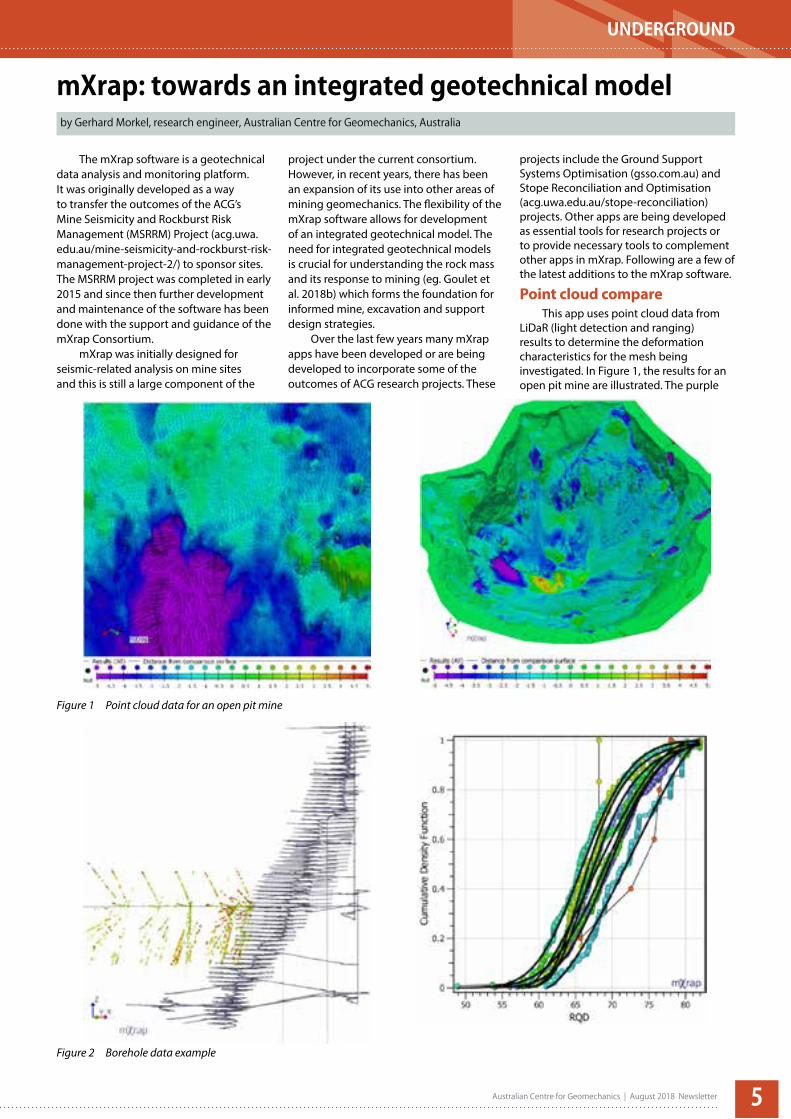
Point cloud compareThis app uses point cloud data from

LiDaR (light detection and ranging) results to determine the deformation characteristics for the mesh being investigated. In Figure 1, the results for an open pit mine are illustrated. The purple

mXrap: towards an integrated geotechnical model by Gerhard Morkel, research engineer, Australian Centre for Geomechanics, Australia

Figure 1 Point cloud data for an open pit mine

Figure 2 Borehole data example

UNDERGROUND


Gerhard Morkel

Australian Centre for Geomechanics, Australia

patches show areas where the pit wall has failed and rock has been displaced, and the yellow/red areas show where the rock has been displaced to.

Borehole dataThe borehole app makes use of a

mine site’s borehole database and provides users with the tools to understand how the rock mass properties change both temporally and spatially. Goulet et al. (2018a) show that parameters typical in a borehole database can provide valuable quantitative and qualitative information for the design of important mine infrastructure in an underground mine with seismicity. Figure 2 is an example of a spatial plot and the cumulative distribution functions (CDFs) of RQD for the different lithologies being considered. For each lithology, the distribution of RQD informs the engineer

of where and what is required in the excavation design.

Sublevel cavingThe sublevel caving app aims to

provide the tools to investigate and analyse the draw and seismic data for a sublevel cave. Typically of interest are the areas of the cave which have been drawn, how much has been drawn and when it was drawn. Such data viewed in conjunction with seismic data, convergence plots from the convergence app, or any other data, provides valuable input in the geotechnical design and monitoring of sublevel caves. For more details see mxrap.com/mxrap-apps/caving-suite/

The ACG has a mandate to improve the geotechnical understanding of the industry and the mXrap platform provides

the technology to make this possible. The consortium of members is gradually growing as the need for understanding more complex rock masses at depth is becoming increasingly common. Visit www.mxrap.com for further details.

Founded in 2015, the mXrap Consortium supports and funds the ACG mXrap software: a geotechnical data analysis and monitoring platform within which data analysis tools are developed.

mXrap Consortium Members

Research MembersAustralian Centre for Geomechanics Perth, Western Australia (The University of Western Australia)Laurentian University Sudbury, CanadaLuleå University of Technology Luleå, SwedenNIOSH Spokane Mining Research Division Spokane, USAUniversidad de Santiago de Chile Santiago, ChileUniversité Laval Quebec, CanadaUniversity of the Witwatersrand Wits, South Africa

mXrap TeamDr Johan WesselooProject Leader

Stuart TierneyPhD Student

Dr Kyle WoodwardResearch Associate

Gerhard MorkelGeotechnical Engineer

Paul HarrisSoftware Engineer

Chun HoPart-time Software Engineer

Dr Dan Cumming-PotvinResearch Associate

• Agnico Eagle Mines Limited, Canada o Goldex o Laronde • Alamos Gold Inc., Canada o Young Davidson• BHP, Australia o Olympic Dam • BHP Nickel West, Australia o Leinster• Boliden Minerals, Sweden o Garpenberg• CMOC Northparkes Mines, Australia o Northparkes Mines• ERM Golden Grove Pty Ltd, Australia o Golden Grove• Glencore Ernest Henry Mining, Australia o Ernest Henry Mine• Glencore Kidd Operations, Canada o Kidd Creek• Glencore - Sudbury Integrated Nickel

Operations, Canada o Nickel Rim South Mine• Goldfields Australia Pty Ltd, Australia o Agnew o Granny Smith o Head Office o Lawlers o South Deep o St Ives • Goldcorp, Canada o Eleonore• Hecla USA, United States of America o Lucky Friday• IAMGOLD Corporation, Canada o Westwood Mine• Independence Group, Australia o Lightning Long Victor

• KCGM (Kalgoorlie Consolidated Gold Mines), Australia

o Mt Charlotte o Super Pit• Kirkland Lake Gold Ltd, Canada o Kirkland Lake• LKAB (Luossavaara-Kiirunavaara AB),

Sweden o Kiruna o Malmberget• MMG Australia Limited, Australia o Head Office o Rosebery • Newcrest Mining Limited, Australia o Cadia Operations o Head Office o Telfer • Newmont Tanami Pty Ltd, Australia o Tanami• Northern Star Resources Ltd, Australia o Hornet o Kanowna Belle o Raleigh • Perilya Limited, Australia o Perilya Broken Hill• PT Freeport Indonesia, Indonesia o Grasberg Server• Red 5 Limited, Australia o Darlot• South32 Cannington, Australia o Cannington• Vale Canada Limited, Canada o Coleman o Creighton o Technical Team• Western Areas, Australia o Flying Fox

PASTE, THICKENED & FILTERED TAILINGS


Current mine waste disposal issues in South Africa and the status of paste and thickened tailingswrites Dr Angus Paterson, Paterson & Cooke, South Africa

The South African mining industry has been through tumultuous times over the last few years, due to a combination of the global commodity crisis and regulatory uncertainty. As a result, there has been a distinct lack of capital projects and the focus has primarily been to reduce operating costs and maintain profitability of existing operations. Andrew Copeland, mining and technical director of Knight Piésold Pty (Limited), South Africa says, “As a result of these two factors, very few operating mines considered changes to their tailings dewatering and pumping systems. In a few cases, clients requested that consultants consider paste and filtered tailings options in the trade-off studies, to compare to thickened tailings solutions, and to confirm whether there was any merit in pursuing them further in the feasibility/detailed design stages.”

A major obstacle to the implementation of thickened and paste tailings in Southern Africa is the significant capital and operating costs of the slurry de-watering and thickening circuits, as well as the costs associated with pumping thick viscous materials. In particular, power costs in South Africa, and specifically in the mining industry, have increased at an annualised average rate of 15.3% per year from 2004 to 2017 (Figure 1). This has had major consequences on operating costs, since projects developed at a cost of ZAR 0.15 per kWh in 2004 are now paying close to R 0.90 per kWh in 2018, a six-fold increase.

In many instances this has meant that the focus has shifted from water saving to power reduction and other general cost-saving measures. Even though Southern Africa is a water scarce region, the relatively low costs and/or scarcity of water alone do not justify the higher costs required to reduce water usage. Compounding the rising operating costs is that changes in the requirements for mine waste disposal have shifted from requiring an approved environmental management plan and water use license to now having to comply with the National Environmental Management Waste Act (NEMWA 2014). This act is broad ranging and is based on the requirements to dispose of domestic waste in landfill sites where liners are required at the base of the landfill. Applying these requirements to mineral waste, that is broadly designated hazardous under the Act, has had significant impacts on the local mining industry in the last few years as the cost

of lining large surface impoundments is prohibitive. Lined impoundments are certainly required in specific instances, but in many cases may not be appropriate, and mines still need to apply for a waste licence as all sites must comply with the Act. As a result of this Act, Copeland says, “Clients have seen a massive jump in capital costs for building new tailings facilities due to legislation that requires they be ‘’lined’’ to protect groundwater. For paste and filtered tailings facilities, lining is still required due to their over-saturated nature (apart from storm events), and their selection would add to the high costs. Typically paste and filtered tailings dewatering and transportation systems require more high-tech management and maintenance, and on more remote mines, this is a significant risk.”

Designing a disposal site to meet the requirements for a safe liner installation requires that a sub-base of suitable material is used as bedding to protect the polyethylene liner that is typically only a few millimetres thick. In some instances, filtered tailings can be used as a suitable base material, as is currently being done on a large facility in South Africa that is now being constructed. Thickened tailings is filtered in fine and coarse fractions at the process plant and the filtered material is trucked to the construction site and placed and compacted on the cleared floor of the basin. Rob McNeill, corporate consultant of SRK's Pietermaritzburg office, says "This method of utilising readily available

materials allows the finer and coarse fraction tailings to be used as bedding and above liner drainage layers respectively significantly lowers construction costs associated with sourcing materials from commercial vendors."

A filtered tailings disposal system has been in operation at Skorpion Zinc Mine in Namibia since 2002 and the decision to use filtered tailings was not only due to the scarcity of water, but the soluble metal credits recovered from the filtrate. Copeland says, “An advancing face conveyor system proved successful over 40 m high filtered tailings. Importantly, the composite slope angles achieved of 30° and 4° are a valuable lesson to designers and demonstrate that these materials, although filtered, remain saturated and will slump and flow to an equilibrium gradient.”

There was a great deal of initial interest in paste and thickened tailings technology in the early 2000s in Southern Africa that saw systems such as the central thickened discharge facility at the De Beers Combined Treatment Plant (CTP) in Kimberly being commissioned, and a high density thickened tailings system installed at the Hillendale heavy minerals mine in Kwa-Zulu Natal. CTP continues to operate as a paste disposal system and the operation has extended beyond the original design life, however the Hillendale Mine ceased operations, as planned, and the majority of the site has been rehabilitated with productive sugarcane land.

R0.00

R0.10

R0.20

R0.30

R0.40

R0.50

R0.60

R0.70

R0.80

R0.90

R1.00

0%

5%

10%

15%

20%

25%

30%

35%

40%

45%

50%

2004/05 2005/06 2006/07 2007/08 2008/09 2009/10 2010/11 2011/12 2012/13 2013/14 2014/15 2015/16 2016/17

Cost

per

kW

h so

ld (Z

AR)

Annu

al a

vera

ge p

rice

adju

stm

ent

Calculated average price adjustment %

Average prices R/kWh sold

Source: http://www.eskom.co.za/CustomerCare/TariffsAndCharges/Pages/Tariff_History.aspx

Figure 1 South African mining industry average power costs since 2004. Source: Eskom Holdings SOC Ltd (2018)



The few high-density tailings disposal operations that continue to operate in South Africa provide valuable lessons to the industry, however the capital costs of paste and filtered tailings remain an obstacle to their feasibility locally and, as a result, very few new designs have been done that use paste and filtered tailings, apart from conventional thickened tailings systems using high rate thickening and centrifugal pumps.

Copeland says, “In Southern Africa, the design and construction of upstream tailings dams remains normal practice because of the lower costs and prevalence of a semi-arid climate, and can be safely constructed if well operated. However, in wetter regions where sun drying and consolidation is not necessarily achieved, alternatives must be considered, and the latest thinking should be incorporated into such studies. Emphasis will be placed on vendors to provide cost-effective, reliable and low maintenance equipment that is easy to operate, otherwise highly technical and capital intensive solutions may give way to traditional ones.” This is a very important statement, as in some instances we see a convergence of capital and operating costs between high-pressure paste pumping and filtered tailings systems. As new filtration technologies

are developed it is expected that this cost differential will further decrease.

However, there is an increasing risk awareness to hydraulically placed tailings due to the well-publicised recent failures of major tailings facilities in Brazil and Canada, and more studies will consider thickened tailings for improved water recovery, but filtered tailings may become the preferred alternative to high pressure paste disposal pumping systems as filtration technology improves.

Figure 2 Filtered tailings prior to placement and compaction

Dr Angus Paterson

Paterson & Cooke, South Africa

8–10 MAY 2019 | THE WESTIN CAPE TOWN | SOUTH AFRICA

22ND INTERNATIONAL CONFERENCE ON

www.paste2019.co.za

MONDAY | 6 MAY TUESDAY | 7 MAY WEDNESDAY | 8 MAY THURSDAY | 9 MAY FRIDAY | 10 MAY

Paterson & Cooke Mine Backfill – Design and

Operation Course

ACG Is the Future Filtered? Paste and Thickened Tailings

Short Course

22nd International Conference on Paste, Thickened and Filtered Tailings

Conference Dinner

ABSTRACTS DUE27 AUGUST

2018

The Australian Centre for Geomechanics is delighted that the 22nd International Conference on Paste, Thickened and Filtered Tailings will be held in Cape Town, South Africa in May 2019, in collaboration with Paterson & Cooke.Conference co-chairs are Professor Andy Fourie, The University of Western Australia and Dr Angus Paterson, Paterson & Cooke.

PASTE, THICKENED AND FILTERED TAILINGS



Polymer-treated tailings: hiding in plain sight

The term thickened tailings is well-known in the tailings management world and has a history that can be traced back to Dr Eli Robinsky’s trial work with conventional thickened tailings at the Kidd Creek copper-zinc mine located in northern Ontario in 1973. However, this term’s direct connection to the more recent term “polymer-treated tailings” is neither well-known nor well-understood by most tailings engineers, especially those without a background in process chemistry. Tailings engineers, many of whom are geotechnical engineers, generally accept that the solids content of tailings delivered to a tailings facility may range between 30 and 60 wt%. However, little thought is typically given to the type of polymer that has been applied in the thickener or other unit process upstream of the deposition spigot to achieve these solids contents. Therefore, it is often not until problems related to fines capture or return water clarity are reported by the mine, that the role and ability of chemistry to effect tailings behaviour is usually considered. Consequently, tailings deposited into tailings storage facilities (TSFs) at base and precious metal mines are often thought of as slurries comprised primarily of water and solids, with the solids subject to hydrodynamic sorting, and some portion of the water reporting for collection and recycle from a supernatant pond.

Yet, anionic copolymers have been used around the mining world for at least two decades to improve dewatering and strength development for a wide range of tailings substrates. For many tailings engineers, thickened tailings are thought of as the underflow product from a thickener, while the term “polymer-treated tailings” has gained increasing attention from process engineers and tailings managers trying to achieve dewatering and consolidation performance that typically exceeds that achieved solely by conventional thickening. This is particularly the case in the treatment of fluid fine tailings in the Alberta oil sands, where anionic polymers are used either on their own, or in combination with coagulants to bind previously dispersed fine-grained particles while liberating water that can be directly reused in the extraction process. However, given the risks and costs associated with tailings management and reclamation, focus is increasingly turning towards quantifying the geotechnical

and environmental performance impacts associated with polymer-treated tailings regardless of where polymer addition occurs.

A shift in focus: from unit process to chemistry plus process

With an increasing requirement to optimise recycling and reuse of process water coupled with a corresponding reduction in the demand in fresh water faced by mining operations the world over, ways to optimise solid-liquid separation while producing water suitable for direct return to the extraction/beneficiation process has gained increasing focus. As such, a steady shift in focus from standalone separation units to polymer-treatment combined with several processes has been observed. In water and energy intensive extraction processes,

like those used to extract bitumen from oil sands ore, it is beneficial to salvage as much of the hot water required in this process as possible before it leaves the extraction plant. Consequently, thickeners at these mine sites often have a primary function of optimising recovery of hot water and utilise only enough polymer as may be required to satisfy this primary objective. Additionally, if the distance between the extraction plant and the tailings disposal area is significant, use of polymer to treat the tailings just prior to depositing them in a TSF (commonly referred to as in-line thickening), can both

minimise pumping costs while potentially increasing the likelihood that the greatest benefits of polymer treatment would be realised within the deposition field.

The larger the mining operation, the larger the amount of waste/tailings produced. Consequently, use of unit processes like filtration or centrifugation can only be entertained at these sites by incurring significant capital expense, meeting the elevated energy demand, and potentially facing penalties for greenhouse gas emissions associated with operating these devices. In addition, when government regulation stipulates that tailings storage deposits must achieve certain geotechnical and environmental performance metrics, mine operators increasingly scrutinise the performance achieved by proposed chemical treatments, as well as the unit processes identified, as possible candidates to help

them achieve the specified objectives.However, in the quest to achieve

specified performance objectives, some process engineers responsible for evaluating systems to achieve these objectives evaluate chemical performance using criteria that does not effectively account for the impact of process kinetics on the polymer candidates being considered (Boxill et al. 2018). This often results in the selection of a polymer that may provide good initial static dewatering but when combined with a high shear process like centrifugation, for example, neither the near-term nor

Characterising the performance potential of polymer-treated tailings

By Dr Lois Boxill, BASF Canada, Canada and John Bellwood BASF plc, UK

Designers, owners and operators of TSFs face ongoing challenges in meeting the needs to safely store large volumes of tailings into the future



long-term dewatering performance can be realised or sustained. This performance gap has prompted some to recognise that, accounting for application, kinetics is an important factor in polymer selection. Additionally, given the sunk capital invested in existing tailings handling infrastructure, operators are increasingly exploring use of polymers to provide secondary treatment of tailings that have likely been thickened at an earlier stage in the process, but which have been degraded because of transporting the treated slurry via pumps and pipelines over several kilometres from the plant to the tailings disposal site. Hence, there is an increasing need to broaden understanding of how any given polymer treats a substrate with a specific range in composition, but also the conditions that support or inhibit the ultimate effectiveness of the selected polymer treatment in the deposition field. Accounting for re-flocculation effectiveness and the need to select a polymer with a wide performance operating window over the range of tailings characteristics anticipated are also critical to identifying and sustaining robust tailings treatment and management throughout a mine’s life.

Evaluating the geotechnical performance of polymer-treated tailings

Thickened tailings technologies have been deployed at alumina refineries and at mine sites around the world processing coal, kimberlite, uranium, phosphate, iron, and poly-metallic ores containing copper, gold, lead, zinc and nickel (Boxill & Hooshiar 2012). During the review of

global thickening operations completed by Boxill and Hooshiar, typical post-thickening solids content ranged between 45 to 63 wt% with solids contents up to 80 wt% achieved at sites utilising deep cone thickening, high-density tailings discharge, central thickened discharge, or high compression filter press technologies (2012).

Use of polymers to treat oil sands fluid fine tailings has been investigated since the late 1970s (Xu & Hamza 2003) and, since the early 2000s, they have been applied to treat these tailings substrates using a range of methods (BGC 2010). However, the most notable difference between application of polymers in conventional thickeners to their application in centrifuges or in in-line thickening is the polymer dose applied. Conventional thickening of fluid fines tailings typically uses polymer doses under 100 g/t of total solids, whereas in-line treatment and centrifugation of similar substrates can start at 400 g/t of total solids and quickly escalate. Consequently, the presence and role of polymers in in-line polymer-treated tailings is more pronounced than in conventional thickening where low polymer doses exist. Furthermore, when polymers are used to treat waste streams of varying characteristics that are impacted by orebody variations, the absence of equipment and personnel to adjust polymer dose in real-time based on the live tailings stream can result in ineffective polymer treatment, with under-dosed and over-dosed conditions resulting. In an under-dosed condition, the clay minerals being targeted are not effectively captured, while in an over-dosed scenario, quantities of hydrated polymer exist in the treated

tailings stream above what is needed to capture the clay minerals targeted.

Therefore, in dewatering unit processes that have been optimised to produce tailings with greater than 40 wt% solids with optimised polymer addition (where required), the resulting thickened tailings are generally considered to be the tailings that must be stored in TSFs designed by geotechnical engineers. Consequently, the full range of engineering parameters have been developed for these thickened tailings. This includes baseline size, engineering strength characterisation and compressibility data that are used to complete the requisite seepage and stability analyses required to confirm acceptable factors of safety for the proposed tailings embankment under a range of operating scenarios. Consequently, in applications like in-line flocculation where the polymer dose tends to be elevated compared to upstream unit processes, the effects associated with inclusion of this additional polymer into tailings systems must be quantified and analysed in terms of overall risk and potential impact on the performance of the receiving TSF.

Creating a robust framework for evaluating polymer-treated tailings

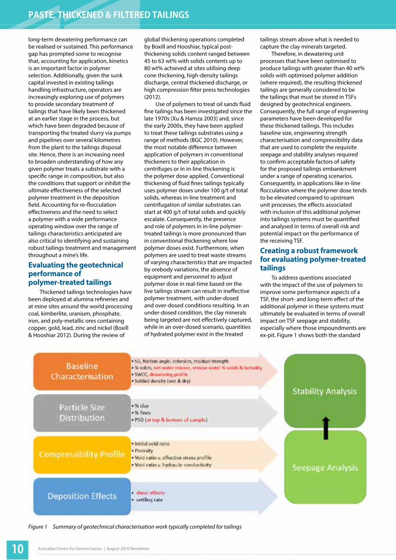
To address questions associated with the impact of the use of polymers to improve some performance aspects of a TSF, the short- and long-term effect of the additional polymer in these systems must ultimately be evaluated in terms of overall impact on TSF seepage and stability, especially where those impoundments are ex-pit. Figure 1 shows both the standard

Figure 1 Summary of geotechnical characterisation work typically completed for tailings



and additional testing and analyses that would be completed to confirm the near- and long-term geotechnical stability of a tailings impoundment.

The actual tests completed should account for the overall performance objectives required of each TSF. Quantifying the effect of increased polymer concentration in a tailings stream addresses persisting questions that geotechnical engineers have about how polymer-treated tailings perform when included in TSFs. Furthermore, completing adequate laboratory-scale testing can provide valuable insight as to any limitations which the proposed treatment may have prior to completing trials at a larger scale.

Closing discussionWith increased awareness of the risks

associated with failure of tailings storage facilities, greater scrutiny of both the embankment design and of all inputs that could potentially impact the geotechnical stability of TSFs should be anticipated. To that end, while polymer-treatment of tailings has been demonstrated to increase water recovery and fines capture on several types of substrates over initial conditions, collection of engineering data and analysis will support greater evaluation by tailings engineers and other stakeholders of the longer-term benefits, potential limitations and considerations associated with use

of polymers to treat tailings in a specific application. By characterising pre- and post-polymer treatment characteristics of specific tailings substrates needing to be managed, key questions about net effects on risk, performance, and geotechnical stability can be understood by tailings engineers, mine owners, regulatory reviewers and other stakeholders.

Consideration of polymer treatment of tailings typically arises when enhanced solid-liquid separation or fines capture is desired. Consequently, improving the understanding of how polymers function as part of an engineered tailings deposit not only facilitates quantification of how the specified performance objectives for the tailings storage will be met, but also allows the benefits of polymer treatment to be evaluated in terms of its overall ability to support attainment of the tailings management objectives specified for a given operation. The long-term environmental effects of using polymer treatment are a component of overall performance and should be described within the context of tailings management even though the fundamental structure of the monomers used in these applications is consistent with the monomers that have been certified for use in water treatment. Therefore, by characterising and quantifying both environmental and engineering impacts, the benefits

and limitations of treating a given tailings substrate with a given polymer empowers engineering and environmental professionals charged with the design, stewardship, closure and reclamation of TSFs to evaluate how a given polymer-treated tailings substrate may be exploited to achieve the near and long-term performance objectives set.

Dr Lois Boxill

BASF Canada, Canada

BASF

Principal Sponsor

21st International Seminar on Paste and Thickened Tailings Reportwrites Candice McLennan, Australian Centre for Geomechanics, Australia

The 21st International Seminar on Paste and Thickened Tailings (Paste 2018) was held 11-13 April 2018, at the Rendezvous Hotel Scarborough, in Perth, Western Australia and was attended by close to 240 delegates.

Paste 2018 was a fantastic forum for industry professionals to discuss and share ideas, outcomes and best practice, as well as enjoy the beachside location of the seminar venue.

Prior to the seminar, on Monday 9 April 2018, the Rheology Fundamentals for Slurries and Pastes Workshop was held and facilitated by Dr Fiona Sofra, Co-founder and Managing Director of Rheological Consulting Services and Professor Peter Scales, The University of Melbourne.

On Tuesday 10 April 2018, the Is the Future Filtered? Paste and Thickened Tailings Short Course was facilitated by Professor Andy Fourie, The University of Western Australia.

Over the three days of the Paste 2018 Seminar, 46 presentations were made by

presenters from 13 countries globally. The presentations covered topics in the paste and tailings arena including thickening and filtration; depositional practices and experiences; transportation; beach profiles; geotechnical aspects; backfill; operational experiences; and new developments.

The keynote speaker on day one was Dr David Cooling from Alcoa Corporation, speaking on ‘Improving the sustainability of residue management practices’. Day two brought with it a keynote presentation from Dr Gordon McPhail of Water, Waste and Land, who spoke on ‘Beach prediction experience to date: further development and review of the stream power-entropy approach’. The final keynote speaker on day three was Dr Michael Davies from Teck Resources whose presentation was on ‘International tailings management guidelines: recent developments’.

The seminar was generously supported by the highly valued sponsors and exhibitors. BASF was the Principal Sponsor, and the Major Sponsors were Active Minerals, Armorpipe Technologies,

FLSmidth, Outotec and Weir Minerals. All of the papers from the Paste 2018

Seminar are openly accessible on the ACG’s Online Repository, with thanks to the open access sponsors, ATC Williams, Feluwa, McLanahan and Paterson & Cooke.

It was announced at the close of the Paste 2018 seminar that the 22nd International Conference on Paste, Thickened and Filtered Tailings will be held in 2019, in Cape Town, South Africa. The ACG will be collaborating with Paterson & Cooke on the organisation of this event.

The ACG team extends warm thanks to all of the delegates, presenters, sponsors and exhibitors who contributed to making Paste 2018 a success.

Paste 2018 marked the last for seminar chair and industry

stalwart, Richard Jewell. Richard was honoured and thanked for

his many years of hard work and dedication.


Within the mining community, geotechnical risk is often underappreciated, sometimes ignored and seldom properly quantified. In all areas of geomechanics, the uncertainty and variability that engineers need to deal with necessitate a rigorous process of quantification or, in the very least, robustly qualifying likelihoods and consequences.

There appears also to be a large gap between the state-of-the-art and the state of general practice when it comes to the qualification and quantification of geotechnical risk. For this reason the Australian Centre for Geomechanics is hosting the First International Conference on Mining Geomechanical Risk (MGR 2019). The aim of the conference is to provide a forum to discuss: the methods used to design for geotechnical risk and those used to manage these risks; to identify shortcomings; and to close the gap between the state-of-the-art and the state-of-practice.

The meaning of riskThe word risk may often be thought

of as an emotive word carrying a negative meaning, with the reaction of having to be avoided at all cost and the idea that opportunity from the flip-side of the “risk coin” is often overlooked. The words “risk assessment” and “risk management” both carry a wide range of possible meanings throughout the mining industry.

On one end of the spectrum, risk is used interchangeably with hazard and is managed by implementing protocols aimed at avoiding any situation that may lead to an adverse outcome. These approaches are better termed “hazard avoidance”. On

the other end, the two components of risk, namely the probability of occurrence and the magnitude of its consequence, are rigorously quantified and decisions are based on considering the risk-reward from balance making use of opportunities that present themselves.

Geomechanical risk encompasses a wide range of probabilities and a wide range of outcomes with severe consequence occurrence often having small likelihood. As a result, geomechanical risk is best dealt with by using quantitative methods.

In general, risk management is a reactive response to geomechanical risk. Design, on the other hand, provides the opportunity to proactively address the geomechanical risks and making use of opportunities by balancing the risk and reward. Within mining, geomechanical risk-based analysis is seldom undertaken.

With geomechanical design, engineers have to design for uncertain and variable conditions and designs are deemed appropriate when they satisfy a defined design acceptance criteria, e.g. a specified factor of safety (FS), probability of failure or a risk level. All three design acceptance criteria have their place within the design and decision-making process as illustrated in Figure 1.

FS as a design criteria is well-known and generally always used even when the other two are employed. Probability of failure (PF) is used to quantify the reliability of a design when faced with uncertainty and variability in the design parameters.

Both the FS and PF focus on stability, i.e. defining a criterion to ensure that when a design is accepted it will be with sufficient

reliability. A design acceptance criterion focused on stability is appropriate for civil engineering structures designed to be stable for long periods with the public having access to these structures.

In mining, personnel safety, rather than ultimate stability, is the aim. Improved safety can be achieved, not only with increasing stability, but with monitoring and the management of personnel exposure.

Personnel exposure can be managed and significantly reduced with the effective use of monitoring. It can be eliminated by remote controlled or autonomously working equipment. In the latter circumstance, for example, a design acceptance criterion focused on stability is not optimum and should be replaced with a criteria that quantifies the financial risk associated with the design. In other circumstances, economic risk and safety risk needs to be evaluated in parallel.

If one considers the fact that mining is about managing the risk-reward balance for the shareholders without endangering its personnel, it is clear that design acceptance criteria in mining should be based on risk and not purely on FS or PF. Risk-based design is not a substitute for probabilistic design, but a continuation of the probabilistic design process taken to its natural conclusion.

Mining geomechanical risk – should we be doing better?The short answer to the question posed in the title of this article is “yes” writes Dr Johan Wesseloo, senior research fellow - rock engineering, Australian Centre for Geomechanics, Australia

Dr Johan Wesseloo

Australian Centre for Geomechanics, Australia

First International Conference on Mining Geomechanical Risk Conference Chair

Geotechnical Design Team

Collect geotechnical data

Interpret data and construct idealised geotechnical model including probabilistic parameter

Choose upper and lower

Perform design assessment

Design meetsacceptance levels

for FS criterion

Choose upper and lower

Perform probabilistic design

Design meets acceptance levels

for PF criterion

Define corporate risk profile

Define acceptance level of

Determine PF threshold resulting in risk below

Evaluate Risks/Reward

Choose final design to maximise shareholder

Owner/Management

Factor of Safety Prob. of failure

Risk

Conceptual design of different alternatives

Optimisation

Implementation

No Yes

Yes Yes

No

Figure 1 Relationship between FS, PF and risk as design acceptance criterion within the design process

Within the mining community, geotechnical

risk is often underappreciated,

sometimes ignored and seldom properly quantified.

UNDERGROUND


A new dynamic test facility for support tendonsby Brendan Crompton, Adrian Berghorst and Greig Knox, New Concept Mining, Australia, Canada and South Africa

The capability with which ground support systems can absorb energy arising from highly stressed, burst-prone or high-deformation mining environments is an increasingly key parameter for the design of a ground support system. It is critical for geotechnical practitioners to have access to sufficient information on the performance of ground support to facilitate informed decision-making whilst designing support standards for mines. Given the high strain rates imposed on support tendons during underground dynamic loading, the laboratory testing of tendons under similar loading rates is beneficial to better understand the behaviour of the support elements. Additionally, access to dynamic test facilities for manufacturers of support units improves the efficiency with which new support units can be developed and qualified for implementation underground.

A number of test methods have been investigated and utilised since initial in situ blasting methods were trialled nearly 50 years ago. These include laboratory-based and in situ underground testing of installed tendons. Different testing methods have provided for dynamic testing of individual support elements, i.e. tendon, faceplate and nut, or larger support systems incorporating a number of support elements acting together.

The laboratory test facilities most commonly used by industry for the dynamic testing of support tendons are in high demand with limited testing capacity which imposes a constraint on the rapid development of new rock support products.

Given the increasing need and benefit in better understanding and designing dynamic support elements, New Concept Mining built a new dynamic test machine, the Dynamic Impact Tester (DIT), at their research facility in Johannesburg, South Africa. Whilst it is accepted that laboratory-

based testing is not fully representative of rockbolt performance when subjected to dynamic loading underground, it is extremely valuable to have the ability to conduct a high number of tests with repeatable parameters to generate sufficient knowledge of the relative performance of different support systems.

The dynamic test machine is designed to test individual tendons (rockbolts and cables), including the faceplate and nut. In accordance with ASTM D7401-08 Standard Test Methods for Laboratory Determination of Rock Anchor Capacities by Pull and Drop Tests (ASTM International 2008), the machine utilises a falling weight impacting on the test sample to impart an energy impulse to the test sample.

Varying the mass and impact velocity of the weight, within the limitations shown in Table 1, allows for testing of different input energies at differing input velocities. This test envelope is illustrated in Figure 3.

A minimum test sample length of 1 m and a maximum sample length of 3.5 m allows for the testing of full size samples for the majority of rockbolt lengths used to support underground mines.

Testing on tendons can be conducted using one of two accepted test configurations. A continuous tube test imparts the impulse directly to the

faceplate of the test sample (Figure 4), whilst a split tube test imparts the impulse indirectly to the test sample by impacting on a strike plate attached to the steel embedment tube at the head of the bolt (Figure 5). A split between the head and toe lengths of the embedment tube simulates a discontinuity in the rock mass. The two different configurations simulate, to some degree, varying behaviour of a rock mass during a dynamic event.

Data interpretation and reporting

During testing, the DIT records a number of variables including displacement at the head and toe of the sample and the impact force applied to the strike plate by the falling weight. Data is collected at a sampling rate of 10 kHz with each data point time stamped to allow accurate correlation of different test parameters for analysis, no data filtering is

Figure 1 Schematic of Dynamic Impact Tester (DIT)

Figure 2 The DIT, as installed

Specification Value

Maximum impulse 65 kJ

Maximum impact velocity

6.42 m/s

Maximum drop mass 3171 kg

Minimum drop mass 551 kg

Maximum drop height 2.1 m

Maximum sample length

3.5 m

Height of structure 8.2 m

Table 1 Test parameter boundaries

Figure 3 DIT test envelope

UNDERGROUND


Figure 4 Continuous tube test Figure 5 Split tube test

applied to the dataset by either hardware or software. A typical example of load and displacement data recorded during a test is shown in Figure 6.

The energy absorbed by the rockbolt during testing is calculated utilising the data captured to perform an energy balance calculation to account for energy losses arising from testing factors such as frictional and acoustic losses. The velocity with which the mass impacts the test sample is calculated theoretically, as per industry practise, but upgrades to the machine are in progress to allow for the accurate measurement of the weight’s velocity during the test event. The calculation of the energy absorbed by the rockbolt is typically represented together with the applied load measured during the event (Figure 7).

In November 2017, Professor John Hadjigeorgiou of the University of Toronto reviewed the testing facilities of the DIT. Following a series of impact tests and analyisis onsite, it was concluded that the facility, procedures and interpretation of results were consistent with international practice of similar rigs. A number of research opportunities using the DIT were also identified.

The frequency with which tests can be conducted on the DIT allows for an increased test rate for both single and multiple impact tests, as well as the rapid processing of test results. Sample preparation comprises the bulk of the lead time required to complete testing. Subject to material availability, resin or friction anchored units require a minimum of three days' preparation and grouted units require a minimum of seven days due to curing of the grout. Prepared samples can be tested at a rate of three to six samples per day, depending on the test configuration and failure mode of the test samples.

The ability to conduct a large number of tests provides the opportunity to rapidly increase the knowledge base on the dynamic performance of support elements. Over a period of six months in 2017, the DIT performed 179 dynamic tests on a number of different tendon configurations. The quick turnaround time between tests is particularly noticeable when conducting

multiple impact tests (Figure 8).The increase in test reports available

for dynamic support units will provide geotechnical practitioners with greater confidence in the consistency with which support elements will behave under a set of loading conditions. Figure 9 plots the behaviour of four identical test samples, each subjected to five dynamic events during testing. Comparison of each test

sample’s load deformation curve provides the insight needed on the reliability of the particular support element.

An added advantage of the DIT is the inclusion of a high definition camera that allows for the live streaming of tests globally over a secure online connection. This allows larger teams to witness the dynamic testing of tendons without the expense or time required to travel to the

Figure 6 Typical load and displacement data from a single drop

Figure 7 Typical load and cumulative energy absorption from a single event

UNDERGROUND


test facility.

Path forwardWith a testing capability between 8

and 65 kJ on a single event at a maximum impact velocity of 6.42 m/s, and equipped with state-of-the-art instrumentation, the DIT offers the geotechnical community the opportunity to gain a better understanding of the dynamic performance of support elements.

Figure 8 Typical load and cumulative energy absorption from multiple events

Figure 9 Multiple event testing on four samples

“It is critical for geotechnical practitioners to have access to sufficient information on the

performance of ground support to facilitate informed

decision-making whilst designing support standards

for mines.”

Brendan Crompton

New Concept Mining, Australia

ACG Corporate Affiliate Memberships

2018 Corporate Affiliates

ACG Corporate Affiliate Memberships allow your company to gain exposure to industry leaders while also providing savings on our well-known and respected further education and training platform. Email [email protected] for details.


RESEARCH

The crack growth mechanism in biaxial compression – what happens on a face or sidewall of a drive?by Hongyu Wang, PhD student, Australian Centre for Geomechanics, The University of Western Australia, Australia

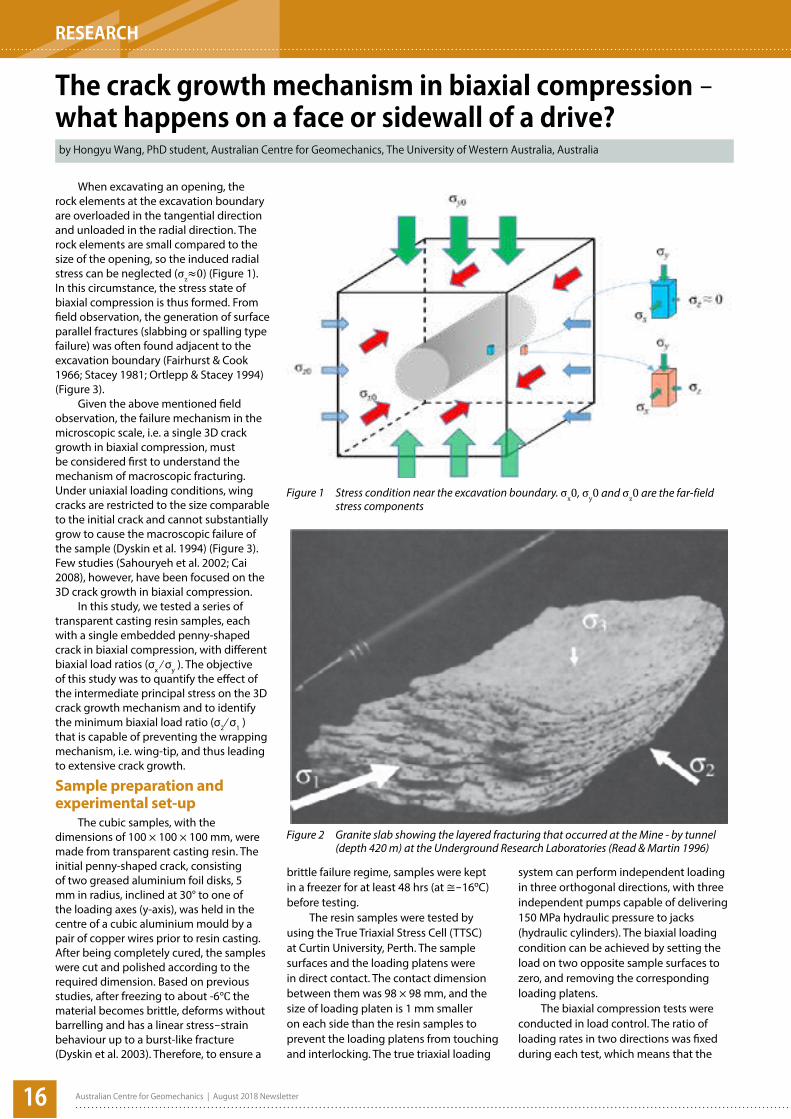
When excavating an opening, the rock elements at the excavation boundary are overloaded in the tangential direction and unloaded in the radial direction. The rock elements are small compared to the size of the opening, so the induced radial stress can be neglected (σz≈0) (Figure 1). In this circumstance, the stress state of biaxial compression is thus formed. From field observation, the generation of surface parallel fractures (slabbing or spalling type failure) was often found adjacent to the excavation boundary (Fairhurst & Cook 1966; Stacey 1981; Ortlepp & Stacey 1994) (Figure 3).

Given the above mentioned field observation, the failure mechanism in the microscopic scale, i.e. a single 3D crack growth in biaxial compression, must be considered first to understand the mechanism of macroscopic fracturing. Under uniaxial loading conditions, wing cracks are restricted to the size comparable to the initial crack and cannot substantially grow to cause the macroscopic failure of the sample (Dyskin et al. 1994) (Figure 3). Few studies (Sahouryeh et al. 2002; Cai 2008), however, have been focused on the 3D crack growth in biaxial compression.

In this study, we tested a series of transparent casting resin samples, each with a single embedded penny-shaped crack in biaxial compression, with different biaxial load ratios (σx ⁄ σy ). The objective of this study was to quantify the effect of the intermediate principal stress on the 3D crack growth mechanism and to identify the minimum biaxial load ratio (σ2 ⁄ σ1 ) that is capable of preventing the wrapping mechanism, i.e. wing-tip, and thus leading to extensive crack growth.

Sample preparation and experimental set-up

The cubic samples, with the dimensions of 100 × 100 × 100 mm, were made from transparent casting resin. The initial penny-shaped crack, consisting of two greased aluminium foil disks, 5 mm in radius, inclined at 30° to one of the loading axes (y-axis), was held in the centre of a cubic aluminium mould by a pair of copper wires prior to resin casting. After being completely cured, the samples were cut and polished according to the required dimension. Based on previous studies, after freezing to about -6℃ the material becomes brittle, deforms without barrelling and has a linear stress–strain behaviour up to a burst-like fracture (Dyskin et al. 2003). Therefore, to ensure a

brittle failure regime, samples were kept in a freezer for at least 48 hrs (at ≅–16oC) before testing.

The resin samples were tested by using the True Triaxial Stress Cell (TTSC) at Curtin University, Perth. The sample surfaces and the loading platens were in direct contact. The contact dimension between them was 98 × 98 mm, and the size of loading platen is 1 mm smaller on each side than the resin samples to prevent the loading platens from touching and interlocking. The true triaxial loading

system can perform independent loading in three orthogonal directions, with three independent pumps capable of delivering 150 MPa hydraulic pressure to jacks (hydraulic cylinders). The biaxial loading condition can be achieved by setting the load on two opposite sample surfaces to zero, and removing the corresponding loading platens.

The biaxial compression tests were conducted in load control. The ratio of loading rates in two directions was fixed during each test, which means that the

Figure 1 Stress condition near the excavation boundary. σx0, σy0 and σz0 are the far-field stress components

Figure 2 Granite slab showing the layered fracturing that occurred at the Mine - by tunnel (depth 420 m) at the Underground Research Laboratories (Read & Martin 1996)


RESEARCH

predefined biaxial load ratio (σx ⁄ σy ) can be maintained within the accuracy of the control module of hydraulic pumps during the whole testing process.

Experimental resultsFigure 4 shows the wing crack surfaces

from the top view with σx ⁄ σy ratio of 0.065, 0.06, 0.0575 and 0.0571, respectively. It is seen that unlike the wrapping phenomenon in uniaxial compression, see Figure 3, the wing cracks were prevented from wrapping, and therefore were able to grow extensively parallel in both loading directions. In addition, with the decrease of the σx ⁄ σy ratio, the flatness of the wing crack surface was increasingly disturbed. At the boundary of the wing crack surface, the tendency of inward curling was shown. Most importantly, the continuity of the wing crack near the initial crack was affected. When the σx ⁄ σy ratio was 0.0575, the wing crack at this point started to show discreteness instead of forming a continuous plane. This observation indicates the transition process from the extensive crack growth pattern to the restricted one.

The restricted wing crack growth was produced when the σx ⁄ σy ratio was ≤0.0567 from test no.11, and repeated in test no.16. The results are shown in Figures 5 (a) and (b), respectively. From test no.11, the restricted mode of wing crack growth was presented. Increasingly the loading time in test No.16, with the same σx ⁄ σy ratio, only led to the limited, noticeable elongation and the progressive failure of the resin material, which was also not attributed to the wing crack growth according to the comparison shown in Figure 5. Hence, we regarded the σx ⁄ σy ratio of 0.057 as the critical value for extensive crack growth under biaxial compression.

DiscussionIn uniaxial compression, or in biaxial

compression when the σx ⁄ σy ratio is below the critical value, the orientation of wing crack growth is only subject to the direction of the major principal stress (σy in this case). No or negligible restriction of forming a crack with preferred orientation, with regard to the direction of two other principal stresses (σx and σz ), exists. The curly crack surface, i.e. wrapping of the

wing crack growth is thus formed and restricts itself to grow substantially along the direction of σy. When the intermediate principal stress (σx in this case) is applied, crack initiation in the direction perpendicular to σx can be suppressed to some extent, depending on the ratio of two loading stresses. When the σx ⁄ σy ratio is high enough, at least above the critical value, the wrapping mechanism can be suppressed, which gives rise to extensive crack growth. In this circumstance, cracks are thus mainly formed and propagate in a preferred orientation, i.e. parallel to both σy and σx (Figure 4).

ConclusionThe results of this research reveal

the transition process of the extensive crack growth mode to the restricted one. Unlike the restricted crack growth in uniaxial compression where the growth is restrained by the wrapping mechanism of the wing cracks, in biaxial compression the crack can grow extensively towards both loading axes depending on the applied σx ⁄ σy ratio. The flatness and continuity of the produced wing crack surfaces can be disturbed when the σx ⁄ σy ratio is kept reducing. The critical value of the σx ⁄ σy ratio inducing extensive crack growth is 5.7% from the experimental study, when the inclination angle of the initial crack is 30° to the y-axis.

Figure 3 Limited wing crack growth of each test under uniaxial compression in sample, with inclination angle of initial crack (a) 30°; (b) 45°

(a)

(b)

Figure 4 Crack growth from top view in biaxial compression with an σx ⁄ σy ratio of: (a) 6.5%; (b) 6%; (c) 5.75%; and (d) 5.71%


RESEARCH

Hongyu Wang

Australian Centre for Geomechanics, The University of Western Australia, Australia

In biaxial compression, above the critical value of the σx ⁄ σy ratio, the intermediate principal stress (σx in this case) suppresses the wrapping mechanism and gives rise to extensive crack growth. It is astonishing that the magnitude of the second compressive stress – the intermediate principal stress – does not need to be high. Wing wrapping can be prevented by the intermediate principal stress as low as 5.7% of the major principal stress (for initial penny-shaped cracks inclined at 30° to the major principal stress direction), which indicates the importance of the intermediate principal stress in the mechanics of fracturing.

Future researchIn the current experimental study,

the inclination angle of the initial crack was limited to 30°. In rock, the initial micro-cracks are randomly oriented, ubiquitous and of the size comparable to that of the structural element. In this way, the macroscopic failure of rock could involve the initiation, propagation and coalescence of multiple cracks. Thus, in the future study entitled, “3D Crack Growth in Biaxial Compression”, Professors Phil Dight and Arcady Dyskin, and

PhD student Hongyu Wang, The University of Western Australia, will conduct more tests with various inclination angles of the initial crack to explore the crack growth phenomenon. In addition, a sample with two or more cracks will be prepared and tested to reveal the crack coalescence mechanism.

Figure 5 Crack growth from lateral view in biaxial compression with an σx ⁄ σy ratio of 5.67%. (a) test no. 11; (b) test no.16

The ACG's Online Repository – growth and opportunitywrites Candice McLennan, Australian Centre for Geomechanics, Australia

In early 2017, the Australian Centre for Geomechanics launched the ACG Online Repository for Conference Proceedings. Since 2005, the ACG has published conference papers across the geotechnical mining spectrum, including underground and open pit mining, paste and thickened tailings and mine closure. The repository aims to provide the mining geomechanics fraternity with open access, peer-reviewed conference proceedings that may assist readers to maintain and develop their skills, knowledge and capabilities.

One year on from the launch date, the repository has grown considerably, as has its audience. There are also exciting plans in place for the development of the platform to include more offerings and opportunities for sponsors to promote their support of the ACG.

In the past year, the ACG team has worked to gain the approval for and publish online many papers from previous conference proceedings, dating back to 2008. This work will continue with the hopes that the majority of our back catalogue of event publications will be freely available on the online repository. The repository has also been promoted to universities throughout the world, along with relevant industry associations.

In addition to this, recent event proceedings have been published on the online repository, including Deep Mining 2017, Paste 2017, Underground Mining Technology 2017 and Paste 2018. Moving forward, all future ACG international event proceedings will be published on the online repository.

Recent Google Analytics reports reflect that since its inception, the repository has received nearly 21,000 sessions from users all over the world, with Australia, North America/Canada and China being the top countries. (Source: www.google.com/analytics/)

LinkedIn has provided the most referrals to the repository, with other social avenues including Facebook, ResearchGate and Twitter. The ACG website and ACG events websites provide a fair amount of the traffic to the repository, as well as scholar.google.com.

As more authors have their work published on the site, and have the link to share and promote on their own social networks, we should see the traffic from sites like LinkedIn and ResearchGate grow even more.

Looking to future plans for the online repository, a number of initiatives will be implemented. From ensuring all

publications comply with ISSN and DOI protocols and widening the range of papers available on the site, to developing scope for sponsorship and promotional opportunities for ACG supporters and affiliates, the ACG endeavours to maximise the full potential of the platform.

View the site at papers.acg.uwa.edu.au. Your feedback is welcome.

The ACG thanks the following Open Access Sponsors of our recent events who have helped us launch, maintain and continue to grow the online repository in order to provide the best possible open access service to industry and academia alike:

• ATC Williams

• Feluwa Pumpen

• McLanahan Corporation

• Paterson & Cooke

• SRK Consulting

https://papers.acg.uwa.edu.au

OPEN PIT


Quantitative evaluation of economic risk for pit slope designby Luis-Fernando Contreras, SRK Consulting (South Africa) Pty Ltd, South Africa

The pit slope design process described in this article is based on a quantitative risk evaluation of the slopes, which has as a central element, the construction of a risk map that relates the probability of the impact to its magnitude. In this process, the economic impacts of slope failure are calculated and used as the elements on which to apply the acceptability criteria for design.

The proposed methodology is an evolution of the approach described by Tapia et al. (2007) and Steffen et al. (2008), where event tree analysis similar to that used for safety risk evaluations was applied to the economic assessment of slope

failures. This approach was superseded by a probabilistic method with a less subjective basis, as described by Contreras and Steffen (2012). The method was still in a development phase at the time of the latter publication, and was due to be applied to actual projects. Later, the methodology was used to evaluate two open pit mine projects, and as a result of that work some improvements were implemented for the construction of the risk map. The updated methodology is described by Contreras (2015) using the two worked projects for illustration purposes. The material presented in this article is extracted from the latter publication.

Proposed methodologyThe proposed risk evaluation process

for slope design is intended to quantify the impact of potential slope failures on the economic performance of open pit mines. Figure 1 illustrates the risk evaluation process and depicts the main elements of the methodology. The diagram includes the main components of the conventional geotechnical slope design process as described in Stacey (2009) and incorporates the additional elements required from the mine design process.

The main objective of the methodology is the definition of the pit slope angles for mine design by applying project specific criteria to the quantified risk costs. The approach includes the following main steps:

• Definition of the set of slope sections for analysis covering key and critical pit areas during the mine life to provide representative cases of potential risks of slope failure within the mine plan.

• Calculation of the probability of failure (PF) of the slopes from the analysis of stability of the selected slope sections.

• Quantification of the economic impacts of slope failure with reference to the loss of annual profit or total project value as measured by the NPV.

• Integration of the results of probability of failure and economic impact on an annual basis to define the economic risk map per year and for the life-of-mine (LOM).

• Comparison of the risk map with criteria to assess acceptability of the design and to define risk mitigation options as required.

• If the analysis is intended for the comparison of alternative slope design options, the process is repeated for each alternative pit layout and the results are collated in a graph of slope angle versus value and risk cost where the optimum slope angles can be defined.

A complete risk evaluation process should also include the evaluation of the safety impact of slope failures. Safety risk evaluation is discussed by Contreras et al. (2006), Terbrugge et al. (2006), Tapia et al. (2007), and Steffen et al. (2008).

Slope sections for analysisThe risk evaluation process requires

a programme of slope stability analyses, including the critical pit areas and years, Figure 2 Realisation of value with time as a criterion for defining years of risk model analysis

Figure 2

ACG article figures

0

2,000

4,000

6,000

2010 2015 2020 2025 2030

Cum

ulat

ive

Prof

it M

$

Year

Periods for Risk Model Analysis

Cumulativeundiscounted profit

Cumulativediscounted profit(DR 10%)Years for riskmodel analysis

Periods for riskmodel analysis

NPV

Figure 1 Risk-based slope design approach

OPEN PIT


in terms of potential economic impacts of eventual slope failures. This means that besides adequate information on geotechnical conditions defining the likelihood of failures, a good understanding of the mine plan is required to identify those areas and years in which the impacts of failure are likely to be greater.

The selection of the sections for stability analysis starts with the selection of the years of the mine life that represent development periods in the mine plan with similar characteristics in terms of pit geometry, production profile, and economic scenario. Figure 2 shows an example of the cumulative discounted profit of a mine plan, which is a representation of the realisation of value with time. This graph facilitates the definition of the appropriate periods and representative years of mine development for the risk model analysis which, in this example, corresponds to the six years defining the stepped curve.

In general, probabilities of failure increase through the mine life, whereas impacts tend to maintain their levels or even decrease as mining progresses. The assumption that risk conditions of a later year (2027) represent those of early years (2025/2026) is therefore reasonable, with a minor effect on the results or, more commonly, on the conservative side. The graph in Figure 2 implies that there is a trade-off between rigour and practicality when selecting the years for analysis. Ideally, every year would have to be analysed, although this would not be practical and is probably unnecessary in the majority of cases.

The appropriate slope sections for analysis can be selected by examination of the mine plan in the identified key years. The criterion used for this selection is based on covering the anticipated higher risk areas of the mine, which include locations where the likelihood of slope failure or the associated impact is expected to be high. Examples of the preferred locations for analysis include areas with higher or steeper slopes, sites with unfavourable geological conditions, areas with distinct characteristics such as those defined by the geotechnical domains, critical access points to mining faces, areas close to key infrastructure, and so forth. The pit development plan sketched in Figure 3 shows an example with the selection of 42 sections used in this article to illustrate the risk process.

Slope stability analysisThe results of the slope stability

analyses are reported in terms of PF values, which are calculated with the appropriate slope stability models in accordance with the relevant failure mechanisms in each domain. The methodology used for the

calculation of the PF is in part determined by the type of deterministic model used for the calculation of the factor of safety (FS) of the slope. A compilation of the methods commonly used in slope design can be found in Lorig et al. (2009).

Due to practical limitations, the PF values calculated with slope models are typically the result of considering the uncertainty of the strength properties of rock masses and structures, without consideration of any other potential factors contributing to slope instability. Therefore, these PF values are incomplete representations of the likelihood of failure, and need to be adjusted for the purpose of a risk consequence analysis, as discussed by Contreras (2015). The first adjustment refers to the estimation of the PF of the pit wall from the calculated PF of the section representing that wall. The second adjustment corresponds to the estimation of the total PF accounting for aspects not included in the calculation of the model PF such as groundwater, geology, mining or seismic events. The model PF typically accounts only for the uncertainty of the material properties. Model uncertainty

Figure 3 Example of selection of slope sections for risk analysis

Figure 4

ACG article figures

Interrupted access to mining faces

Covered ore

Slope failure impacts:- Disruption of planned ore feed to plant.- Additional costs to restore site. Failure impact = NPVreference – NPVwith failure

failu

re

Figure 4 Conceptual basis for estimation of the economic impact of slope failure

OPEN PIT


is an additional aspect that needs to be considered in the evaluation of the PF for a risk study and refers to the calibration of the calculated FS against actual frequency of slope failures. However, the lack of local historic records leads to the use of judgement to account for this uncertainty.

Economic impact of slope failure events

The economic impact of a slope failure can be measured through the quantification of the effect of this event on the value of the mine plan as measured by the NPV. The NPV corresponds to the cumulative discounted annual profits during the LOM and is normally defined as the result of a mining scheduling and optimisation process carried out with specialised software. In general, the economic impact of a slope failure is a result of the disruption of the planned ore feed during the time required to restore the site, and the additional costs caused by these activities. Figure 4 illustrates the conceptual basis for the estimation of impacts of slope failures. The economic impact of a slope failure is defined as the

difference between the NPV of reference (mine plan without failures), and the re-calculated NPV incorporating the effects of the failure on production and cost components.

Production may be disrupted by different factors such as interrupted access to the mining faces, covered ore, variations

of grade when alternative sources of ore are used to mitigate the effects of the failure etc. The extra costs are caused by the additional material handling and rescheduling of equipment required to restore the site affected by the failure.

A simplified approach to quantifying the impact of a failure consists of

Figure 5 Structure of simplified cash flow model for slope failure assessment

ACG article figures

2015 … 2017 … 2027 2015 … 2017 … 2037ProductionWaste kt 100,000 … 100,000 … 100,000 100,000 … 100,000 … 100,000Ore kt 20,000 … 20,000 … 20,000 20,000 … 20,000 … 20,000Total tonnes kt 120,000 … 120,000 … 120,000 120,000 … 120,000 … 120,000Plant product tonnes kt 160 … 160 … 160 160 … 160 … 160

Failure Impact on ProductionSize of failure kt 0.0 … 0.0 … 0.0 0.0 … 6,150 … 0.0Failure impact factor % 0% … 0% … 0% 0% … 8% … 0%Plant product tonnes after impact kt 160 … 160 … 160 160 … 148 … 160

RevenueForecasted metal price $/lb 3 … 3 … 3 3 … 3 … 3Total revenue M$ 1,390 … 1,390 … 1,390 1,390 … 1,325 … 1,390

CapexTotal Capex M$ 32 … 32 … 32 32 … 32 … 32

OpexFixed Opex M$ 140 … 140 … 140 140 … 140 … 140Variable Opex M$ 561 … 561 … 561 561 … 561 … 561Unit Opex $/t 2 … 2 … 2 2 … 2 … 2Total Opex M$ 701 … 701 … 701 701 … 701 … 701

Failure Impact on CostsUnit cost failure clean up $/t 6 … 6 … 6 6 … 6 … 6Additional costs failure repair M$ 0 … 0 … 0 0 … 37 … 0

ProfitUndiscounted profit per year M$ 657 … 657 … 657 657 … 555 … 657Discount rate 10%Discounted profit per year M$ 543 … 449 … 173 543 … 379 … 173Cumulative discounted profit M$ 1,140 … 1,746 … 4,843 1,140 … 2,014 … 4,773

NPV of reference 5,000 M$ NPV with failure 4,930 M$ Event No. 3Estimated failure impact 70 M$ Year of failure 2017

Item Unit Cash Flow of Reference Cash Flow with Slope Failure

Figure 6 Event tree for economic impact of slope failure of pit with two major slopes

ACG article figures

5% 100 10% 50 0.5% 150

5% 100 90% 0 4.5% 100

95% 0 10% 50 9.5% 50

95% 0 90% 0 85.5% 0

check 100.0%Input Data

P I5% 100

10% 50

E slope fails

West

East slope performance

West slope performance

Pit Performance year i

SlopeEast

E slope stable

E slope stable

W slope stable E fails

W slope fails

W slope stable No failures

W fails

E slope fails W slope fails E + W fail

Pit slopes exposed year i

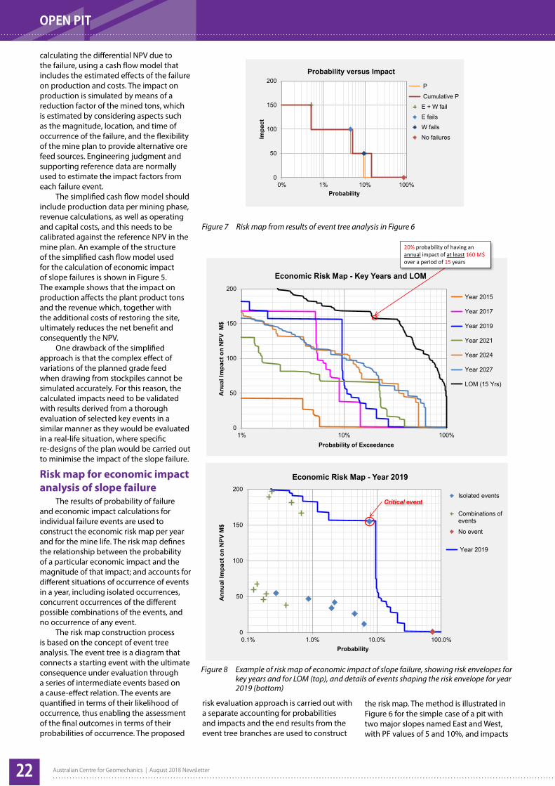
OPEN PIT


calculating the differential NPV due to the failure, using a cash flow model that includes the estimated effects of the failure on production and costs. The impact on production is simulated by means of a reduction factor of the mined tons, which is estimated by considering aspects such as the magnitude, location, and time of occurrence of the failure, and the flexibility of the mine plan to provide alternative ore feed sources. Engineering judgment and supporting reference data are normally used to estimate the impact factors from each failure event.

The simplified cash flow model should include production data per mining phase, revenue calculations, as well as operating and capital costs, and this needs to be calibrated against the reference NPV in the mine plan. An example of the structure of the simplified cash flow model used for the calculation of economic impact of slope failures is shown in Figure 5. The example shows that the impact on production affects the plant product tons and the revenue which, together with the additional costs of restoring the site, ultimately reduces the net benefit and consequently the NPV.

One drawback of the simplified approach is that the complex effect of variations of the planned grade feed when drawing from stockpiles cannot be simulated accurately. For this reason, the calculated impacts need to be validated with results derived from a thorough evaluation of selected key events in a similar manner as they would be evaluated in a real-life situation, where specific re-designs of the plan would be carried out to minimise the impact of the slope failure.

Risk map for economic impact analysis of slope failure

The results of probability of failure and economic impact calculations for individual failure events are used to construct the economic risk map per year and for the mine life. The risk map defines the relationship between the probability of a particular economic impact and the magnitude of that impact; and accounts for different situations of occurrence of events in a year, including isolated occurrences, concurrent occurrences of the different possible combinations of the events, and no occurrence of any event.

The risk map construction process is based on the concept of event tree analysis. The event tree is a diagram that connects a starting event with the ultimate consequence under evaluation through a series of intermediate events based on a cause-effect relation. The events are quantified in terms of their likelihood of occurrence, thus enabling the assessment of the final outcomes in terms of their probabilities of occurrence. The proposed

risk evaluation approach is carried out with a separate accounting for probabilities and impacts and the end results from the event tree branches are used to construct

the risk map. The method is illustrated in Figure 6 for the simple case of a pit with two major slopes named East and West, with PF values of 5 and 10%, and impacts

Figure 7 Risk map from results of event tree analysis in Figure 6

ACG article figures

0

50

100

150

200

0% 1% 10% 100%

Impa

ct

Probability

Probability versus Impact

P Cumulative PE + W failE failsW failsNo failures

Figure 8 Example of risk map of economic impact of slope failure, showing risk envelopes for key years and for LOM (top), and details of events shaping the risk envelope for year 2019 (bottom)

ACG article figures

0

50

100

150

200

1% 10% 100%

Anua

l Im

pact

on

NPV

M$

Probability of Exceedance

Economic Risk Map - Key Years and LOM

Year 2015

Year 2017

Year 2019

Year 2021

Year 2024

Year 2027

LOM (15 Yrs)

20% probability of having anannual impact of at least 160 M$over a period of 15 years

Figure 8 part 1

ACG article figures

0

50

100

150

200

0.1% 1.0% 10.0% 100.0%

Annu

al Im

pact

on

NPV

M$

Probability

Economic Risk Map - Year 2019

Isolated events

Combinations ofevents

No event

Year 2019

Critical event

Figure 8 part 2

OPEN PIT


of 100 and 50, respectively. The sum of the probabilities of the four possible outcomes depicted with the tree is 100%, indicating that all the possible combinations of events have been adequately accounted. The risk map constructed with the results of the event tree is shown in Figure 7. The cumulative probability curve of particular impacts constitutes the economic risk envelope of the pit.

The risk map of a more realistic case, such as the mine plan described in Figures 2 and 3, is constructed for the individual key years selected to represent the various periods of the mine plan, which are then used to define the overall risk map for the LOM (Figure 8). The graph at the top shows the various risk envelopes and the graph at the bottom shows the details of the failure events of year 2019 used to construct the envelope. The risk envelopes are cumulative probability distributions of impacts and are interpreted as indicated in the graph at the top of Figure 8, for the case of impacts with a 10% probability of exceedance. The result for the indicated case would be a 20% probability of having an annual impact of at least $160 million over a period of 15 years. The display of the individual events in the risk chart is useful to identify critical events causing an increase of the risk level as measured by the envelope, as depicted in the example shown on the graph at the bottom of Figure 8.

Probability concepts for construction of risk map

The slope failure events considered for the construction of risk maps correspond to large-scale failures and are analysed on a year-by-year basis. The events are treated as Bernoulli trials and are characterised by a probability of occurrence (p) given by the calculated probability of failure of the slope (PF) and the respective impact (i) estimated in monetary terms. The risk map construction is based on the calculation of

the probability (p) of having an economic impact (i), considering different possible situations of occurrence of the events.

In the following expressions, the terms with sub-indices i, j, and k (in bold) represent the occurring events, and those with sub-indices r, s, and t (in italic), refer to the non-occurring events: Occurrence of single events:

Multiple occurrence of events:

A particular case of the multiple occurrence described in equation [2] is the occurrence of all the events in a year:

No occurrence of any of the events:

The total number of possible cases of occurrence of events (T) for (n) independent events in a year, effectively corresponds to the number of branches of the respective event tree, and is given by the following expression:

From this number, n cases correspond with the occurrence of isolated events and one case to the non-occurrence of any of the events. The remaining N cases correspond with the occurrence of combinations of two or more events. The generic expression to calculate the number of combinations (N) of two or more events that can be obtained with (n) events is:

or

The calculation of all possible probability and impact pairs can be done

Table 1 Number of possible cases of occurrence for the situation of 7 events per year

8

corresponding cumulative frequency curve, as shown in the graph at the top of Figure 10 for the year 2019 of the example in Table 2.

Table 1 Number of possible cases of occurrence for the situation of 7 events per year

Probabilities and Impacts of combination of eventsDescription No cases P IIsolated events 7 p1.q1.q2.q3.q4.q5.q6 i12 events 21 p1.p2.q1.q2.q3.q4.q5 i1+i23 events 35 p1.p2.p3.q1.q2.q3.q4 i1+i2+i34 events 35 p1.p2.p3.p4.q1.q2.q3 i1+i2+i3+i45 events 21 p1.p2.p3.p4.p5.q1.q2 i1+i2+i3+i4+i56 events 7 p1.p2.p3.p4.p5.p6.q1 i1+i2+i3+i4+i5+i67 events 1 p1.p2.p3.p4.p5.p6.p7 i1+i2+i3+i4+i5+i6+i7No event 1 q1.q2.q3.q4.q5.q6.q7 0Total 128

Notes:Numbers identifying the p, q and i terms in the expressions to calculate P and I should be interpreted as indices that are cycled through the 7 individual events to generate the number of cases indicated in column 2.p = probability of failureq = probability of no failure = (1 - p)i = economic impact of individual eventP = probability of occurrence of combination of eventsI = cumulative impact of combination of events

Table 2 Example of data for construction of the risk map for impact on NPV

Year 2015 2017 2019 2021 2024 2027LOM Year 2 4 6 8 11 14

Section PF % Impact M$ PF % Impac

t M$ PF % Impact M$ PF % Impac

t M$ PF % Impact M$ PF % Impac

t M$

1 0.1 109 0.2 72 0.4 55 0.7 52 1.7 54 3.7 592 0.1 78 0.9 96 5.8 26 11.1 64 17.6 62 23.0 523 1.2 25 1.7 70 2.6 34 3.7 27 5.1 35 6.1 294 3.7 41 5.9 36 8.0 12 10.3 15 13.9 43 16.1 605 0.6 16 5.2 166 9.5 155 12.0 65 15.4 68 19.4 446 0.1 18 0.4 92 1.2 47 2.9 14 7.3 48 10.1 407 0.1 14 0.8 83 2.9 42 6.4 11 9.4 43 12.0 34

Note:NPV of reference M$ 5,000

The risk map result is shown in the graph at the bottom of Figure 10. The graph contains the probability distribution plots with the axes swapped to conform with the typical way in which risk acceptability criteria is presented. The graph also includes the data points representing the various possible occurrences of the events. The blue data points correspond with isolated events, the green points with the concurrent occurrence of combinations of events, and the red point on the horizontal axis represents the particular situation of no occurrence of any of the events. Not all the data points are visible because many of them correspond with low probability values outside the range of the logarithmic scale used in the graph.

Nevertheless, these low-probability events have an influence on the final result, which is captured by the cumulative distribution curve. Typically the risk map excludes the frequency distribution histogram in order to avoid an overcrowded graph. A practical way of defining the cumulative distribution curve of impacts is through a Monte Carlo simulation where the seven failure events are modelled with Bernoulli distributions, also called yes-no distributions, and the impacts calculated accordingly.

[3]

[2]

[1]

Table 2 Example of data for construction of the risk map for impact on NPV

Year 2015 2017 2019 2021 2024 2027

LOM Year 2 4 6 8 11 14

Section PF% Impact M$ PF% Impact M$ PF% Impact M$ PF% Impact M$ PF% Impact M$ PF% Impact M$

1 0.1 109 0.2 72 0.4 55 0.7 52 1.7 54 3.7 59

2 0.1 78 0.9 96 5.8 26 11.1 64 17.6 62 23.0 52

3 1.2 25 1.7 70 2.6 34 3.7 27 5.1 35 6.1 29

4 3.7 41 5.9 36 8.0 12 10.3 15 13.9 43 16.1 60

5 0.6 16 5.2 166 9.5 155 12.0 65 15.4 68 19.4 44

6 0.1 18 0.4 92 1.2 47 2.9 14 7.3 48 10.1 40

7 0.1 14 0.8 83 2.9 42 6.4 11 9.4 43 12.0 34

Note: NPV of reference M$ 5,000 (USD)

OPEN PIT


without constructing the respective event tree, which would be a cumbersome task as the number of branches of the tree increases exponentially with the number of annual events. A summary of the probabilities and impacts of the different possible combinations of seven events per year is presented in Table 1. In this table, p corresponds with the probability of occurrence (failure) and q with the probability of no occurrence (no failure) of the respective events. The number of cases in Table 1 is calculated with equation [2] and the total number of possible occurrences of the seven events is 128. This is the number of data points available to construct the risk map.

Construction of the risk mapAn example of the input data required

for the construction of the risk map is presented in Table 2. The data includes the probability of slope failure and the associated impact of seven sections per year and six years of analysis, on the mine plan of 15 years’ duration (Figures 2 and 3). The PF values in Table 2 are based on the results of the geotechnical analysis of the respective sections and cater for the atypical conditions leading to failure not included in those analyses.

The data in Table 2 is shown in graphic form in Figure 9 to illustrate the variations of the probability of failure and associated impacts with pit development. The top graph of Figure 9 is consistent with the increasing likelihood of failure of the slopes expected as the pit grows deeper. The curves in the bottom graph of Figure 9 do not show a unique trend in the variation of impact with pit growth, as impacts are dependent on the particular characteristics of ore exposure and ore access during the development of the mining phases.

The risk map construction is carried out per year and the data is used to calculate the pairs of values of probability and impact associated with all possible combinations of failure events using the expressions in Table 1. The 128 data pairs for each year of analysis

are sorted and used to construct the respective probability distribution graphs of impacts. These graphs include a frequency distribution histogram and the corresponding cumulative frequency curve, as shown in the graph at the left of Figure 10 for the year 2019 of the example in Table 2.

The risk map result is shown in the graph at the right of Figure 10. The graph contains the probability distribution plots

with the axes swapped to conform with the typical way in which risk acceptability criteria is presented. The graph also includes the data points representing the various possible occurrences of the events. The blue data points correspond with isolated events, the green points with the concurrent occurrence of combinations of events, and the red point on the horizontal axis represents the particular situation of no occurrence of any of the events. Not all

Figure 9 Input data for construction of economic risk map, probability of failure of the slopes (top) and impact on NPV (bottom)

ACG article figures

0.1%

1.0%

10.0%

100.0%

2010 2015 2020 2025 2030

PF to

tal

Year

Probability of Failure

1

2

3

4

5

6

7

0.1%

1.0%

10.0%

2010 2015 2020 2025 2030

Impa

ct %

NPV

Year

Impact of Failure on NPV

1

2

3

4

5

6

7

Figure 10 Construction of the economic risk envelope for year 2019 in example from Table 2; probability distribution graphs (left) and risk map result (right)

ACG article figures

0%

1%

10%

100%

20018016014012010080604020

Prob

abili

ty

Annual Impact M$

Probability Distribution of Impact - Year 2019

Frequencydistribution

Prob

abili

ty

100%

10%

1%

0.1%0

Part 1

ACG article figures

0

50

100

150

200

0.1% 1.0% 10.0% 100.0%

Annu

al Im

pact

M

$

Probability

Economic Risk Map - Year 2019Isolated events

Combination ofevents

No event

Frequencydistribution

Cumulativefrequencydistribution

Section 5

Part 2

OPEN PIT


the data points are visible because many of them correspond with low probability values outside the range of the logarithmic scale used in the graph.

Nevertheless, these low-probability events have an influence on the final result, which is captured by the cumulative distribution curve. Typically the risk map excludes the frequency distribution histogram in order to avoid an overcrowded graph. A practical way of defining the cumulative distribution curve of impacts is through a Monte Carlo simulation where the seven failure events are modelled with Bernoulli distributions, also called yes-no distributions, and the impacts calculated accordingly.

The probability values given by the risk envelope should be interpreted as probabilities of exceedance of the respective value, as this curve corresponds

to a cumulative probability distribution associated with all possible combinations of events considered. The risk envelope defines the economic risk profile for the respective year. The analysis of the patterns shown by the data points representing the occurrence of individual events is valuable for identifying critical events that push the risk envelope towards the upper right side of the graph. One example of such an event would be the slope failure associated with Section 5 in year 2019 (Figure 10).

The risk envelopes of the six representative years included in Table 2 were used to construct the economic risk map for the LOM, as shown in the graph at the top of Figure 8. The procedure is based on compounding the probabilities of the various years for fixed values of impact, considering the periods of the mine life represented by each year (Figure 2). The

probability values are added using the concept of reliability of a system. In this particular example, the probability of an economic impact for the LOM (PLOM) for a given impact is calculated from the corresponding annual probabilities using the following expression:

PLOM=1–(1–P2015 )2 (1–P2017)2 (1–P2019)2 (1–P2021)2 (1–P2024)3 (1–P2027)4

The exponents in this equation correspond to the number of years represented by the probability value in the respective term. The sum of these exponents is 15 and corresponds with the total number of years of the mine plan.

A different perspective of the economic risk could be provided by the analysis of impacts on annual profits, because in this way, future amounts are not discounted to present values, which in some cases causes a perceived distortion of value. Risk maps based on the impacts on annual profits can be calculated following a similar process to that described for impacts on NPV. Furthermore, the analysis can be carried out with impacts measured in terms of commodity product rather than monetary units, in order to avoid possible distortions caused by the assumptions on commodity prices.

Uses of the risk mapThere are two main uses of the risk

map: one is for the evaluation of a specific open pit design in terms of economic risk by comparing the result with acceptability criteria; and the second refers to the comparative analysis of open pit design options, in terms of value and risk, to identify optimum pit layouts.Comparison with acceptability criteria

The risk map can be used to assess a specific pit design by comparing this result with acceptability criteria specifically defined for the project. The result of this analysis enables the identification of the more appropriate risk treatment strategies to advance the project. In particular, the comparison with acceptability criteria is

Figure 11 Example of risk acceptability matrix for economic impact (top) and the appropriate risk treatment options (bottom)

ACG article figures

Impa

ct

Level Range M$ Risk Category

5 > 200 H H H H H

4 100 - 200 M M H H H

3 50 - 100 L M M M H

2 10 - 50 L L L M M

1 < 10 L L L L L

Range % <10% 10-20% 20-50% 50-80% >80%

Level 1 2 3 4 5

Likelihood

Impa

ct

Level Range M$ Risk Treatment

5 > 200

4 100 - 200

3 50 - 100

2 10 - 50

1 < 10

Range % <10% 10-20% 20-50% 50-80% >80%

Level 1 2 3 4 5

Likelihood

Avoid risk Transfer risk

Accept risk Reduce risk

Figure 12 Comparison of risk map in Figure 8 with acceptability criteria in Figure 11, for the evaluation of results of individual years (left) and LOM (right)

ACG article figures

0

50

100

150

200

1% 10% 100%

Anua

l Im

pact

on

NPV

M$


Evaluation of Results of Individual Years

Year 2015

Year 2017

Year 2019

Year 2021

Year 2024

Year 2027

LOM (15 Yrs)

Risk Category

High

Moderate

Low

Part 1

ACG article figures

0

50

100

150

200

1% 10% 100%

Annu

al Im

pact

on

NPV

M$


Evaluation of LOM Result

Year 2015

Year 2017

Year 2019

Year 2021

Year 2024

Year 2027

LOM (15 Yrs)

Risk Category

High

Moderate

Low

Part 2

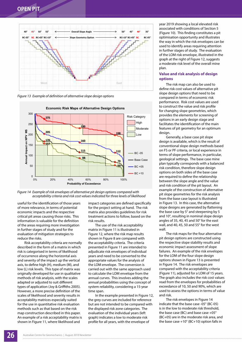
OPEN PIT


useful for the identification of those years of more relevance, in terms of potential economic impacts and the respective critical pit areas causing those risks. This information is valuable for the definition of the areas requiring more investigation in further stages of study and for the evaluation of mitigation strategies to reduce the risks.

Risk acceptability criteria are normally described in the form of a matrix in which risk is categorised in terms of likelihood of occurrence along the horizontal axis and severity of the impact up the vertical axis, to define high (H), medium (M), and low (L) risk levels. This type of matrix was originally developed for use in qualitative methods of risk analysis, with the scales adapted or adjusted to suit different types of application (Joy & Griffiths 2005). However, a more precise definition of the scales of likelihood and severity results in acceptability matrices especially suited for the use in quantitative risk evaluation methods such as that based on the risk map construction described in this paper. An example of a risk acceptability matrix is shown in Figure 11, where likelihood and

impact categories are defined specifically for the project setting at hand. The risk matrix also provides guidelines for risk treatment actions to follow, based on the risk results.

The use of the risk acceptability matrix in Figure 11 is illustrated in Figure 12, where the risk map results shown in Figure 8 are compared with the acceptability criteria. The criteria presented in Figure 11 are intended to adjudicate risk envelopes of individual years and need to be converted to the appropriate values for the analysis of the LOM envelope. The conversion is carried out with the same approach used to calculate the LOM envelope from the annual curves. This involves adding the annual probabilities using the concept of system reliability, considering a 15-year time span.

In the example presented in Figure 12, the grey curves are included for reference but are not intended to be compared with the displayed risk zone categories. The evaluation of the individual years (left graph) indicates a low to moderate risk profile for all years, with the envelope of

year 2019 showing a local elevated risk associated with conditions of Section 5 (Figure 10). This finding constitutes a pit optimisation opportunity and illustrates the way in which the risk envelopes can be used to identify areas requiring attention in further stages of study. The evaluation of the LOM risk envelope, illustrated in the graph at the right of Figure 12, suggests a moderate risk level of the overall mine plan.

Value and risk analysis of design options

The risk map can also be used to define risk cost values of alternative pit slope design options that need to be compared in terms of economic risk performance. Risk cost values are used to construct the value and risk profile for changing slope geometries, which provides the elements for screening of options in an early design stage and facilitates the identification of the main features of pit geometry for an optimum design.

Generally, a base case pit slope design is available, which is the result of conventional slope design methods based on FS or PF criteria, or local experience in terms of slope performance, in particular, geological settings. The base case mine plan typically corresponds with a balanced risk condition, therefore slope design options on both sides of the base case are required to define the relationship between the slope angle and the value and risk condition of the pit layout. An example of the construction of alternative pit slope geometries for the risk analysis from the base case layout is illustrated in Figure 13. In this case, the alternative slope designs are generated by flattening the base case by 5° and steepening by 5 and 10°, resulting in nominal slope design angles of 35, 40, 45 and 50° for the east wall, and 40, 45, 50 and 55° for the west wall.

The risk maps for the four alternative pit design options are constructed using the respective slope stability results and economic impact assessment of slope failures. An example of the risk envelopes for the LOM of the four slope design options shown in Figure 13 is presented in Figure 14. The risk envelopes are compared with the acceptability criteria (Figure 11), adjusted for a LOM of 15 years. The graph also includes the risk cost values read from the envelopes for probabilities of exceedance of 10, 50 and 90%, which are used to assess the options in terms of value and risk.

The risk envelopes in Figure 14 indicate that the base case -05° (BC-05) is in the low to moderate risk threshold, the base case (BC) and base case +05° (BC+05) are in the moderate risk area, and the base case +10° (BC+10) option falls in

Figure 13 Example of definition of alternative slope design options

ACG article figures

BC-05° BC BC+05° BC+10° Slope Geometry Option BC+10° BC+05° BC BC-05°

40° 45° 50° 55° Overall Slope Angle 50° 45° 40° 35°

West East

Figure 14 Example of risk envelopes of alternative pit design options compared with acceptability criteria and risk cost values indicated for three levels of likelihood

ACG article figures

0

50

100

150

200

250

300

0% 20% 40% 60% 80% 100%

Annu

al Im

pact

on

NPV

M$


Economic Risk Maps of Alternative Design Options

BC -05

Base Case

BC +05

BC +10

Risk Category

High

Moderate

Low

275

205

170157

198

112

7053

230

160

115

88

OPEN PIT


the high risk area. The comparison with the acceptability criteria does not provide sufficient elements to establish a clear contrast between the options in terms of their risk performance.

The risk cost values indicated in Figure 14 are used to construct the value and risk profiles of the slope design (Table 3 and Figure 15). These results show the variation of value in terms of NPV and risk cost for the various slope design angles. The design options have been categorised in terms of the risk results as conservative, balanced, aggressive, and maximum, for the slope design cases of BC-05, BC, BC+05, and BC+10, respectively. The risk cost or costs of impact of slope failures have an inverse relationship with the probability of incurring those costs, with higher probabilities of small impacts and lower probabilities associated with large impacts.

The graph at the top of Figure 15

shows the typical increase of risk cost with increasing slope angle for various levels of likelihood of impacts. The risk cost values were used to construct the NPV with risk curves shown in the graph at the bottom of Figure 15. This graph shows a steady increase in NPV with increasing slope angle when no risk aspects are considered. However, once the risk cost is included in the analysis, the curve of value shows an inflexion point as the slope steepens, defining the angle that represents the optimum balance between value and risk. The results in Figure 15 would serve to confirm the adequacy of the base case design, and would suggest a possible optimisation opportunity by steepening the slopes by up to 3°.

Information, such as that included in Figure 15, constitutes a valuable tool to optimise the pit design and to bracket the overall slope angles for further phases of

study.

ConclusionsThe methodology presented provides

a rational approach to defining, at an early stage of a mine, the main features of pit geometry reflecting the appropriate balance between value and risk, in accordance with the specific conditions of the project. The process considers both the likelihood of occurrence of individual slope failure events and the resulting economic impacts from all possible combinations of occurrence of these events on an annual basis and for the mine life.

The economic risk map constructed for a particular pit slope layout can be used in an optimisation process by comparing this result with project-specific acceptability criteria. When the process is used for the evaluation of alternative design options, the risk maps can be used to make risk cost estimations to calculate the variation of project value with slope angle. These results enable the definition of the main features of pit geometry reflecting the appropriate balance between value and risk, in accordance with the specific conditions of the mine, which allows the rationalisation of requirements of geotechnical information at different stages of project development, once risk criteria have been defined.

AcknowledgementThis article has been extracted with

kind permission of the Southern African Institute of Mining and Metallurgy from the article published in the July 2015 edition of the SAIMM Journal, Volume 115.

Luis-Fernando Contreras

SRK Consulting (South Africa) Pty Ltd, South Africa

Table 3 Value and risk cost of the pit design options

12

Figure 13 Example of definition of alternative slope design options

Figure 14 Example of risk envelopes of alternative pit design options compared with acceptability criteria and risk cost values indicated for three levels of likelihood

The risk envelopes in Figure 14 indicate that the base case -05° (BC-05) is in the low to moderate risk threshold, the base case (BC) and base case +05° (BC+05) are in the moderate risk area, and the base case +10° (BC+10) option falls in the high risk area. The comparison with the acceptability criteria does not provide sufficient elements to establish a clear contrast between the options in terms of their risk performance.

The risk cost values indicated in Figure 14 are used to construct the value and risk profiles of the slope design (Table 3 and Figure 15). These results show the variation of value in terms of NPV and risk cost for the various slope design angles. The design options have been categorised in terms of the risk results as conservative, balanced, aggressive, and maximum, for the slope design cases of BC-05, BC, BC+05, and BC+10, respectively. The risk cost or costs of impact of slope failures have an inverse relationship with the probability of incurring those costs, with higher probabilities of small impacts and lower probabilities associated with large impacts.

Table 3 Value and risk cost of the pit design options

Case No

Slope Angle Option

(°)

Design Class

NPV (M$)

Risk Cost (M$) NPV with risk (M$)

P 10% P 50% P 90% P 10% P 50% P 90%

1 BC -05° conservative 4,935 157 88 53 4,778 4,847 4,8822 BC balanced 5,000 170 115 70 4,830 4,885 4,9303 BC+05° aggressive 5,050 205 160 112 4,845 4,890 4,9384 BC+10° maximum 5,090 275 230 198 4,815 4,860 4,892

The graph at the top of Figure 15 shows the typical increase of risk cost with increasing slope angle for various levels of likelihood of impacts. The risk cost values were used to construct the NPV with risk curves shown in the graph at the bottom of Figure 15. This graph shows a steady increase in NPV with increasing slope angle when no risk aspects are considered. However, once the risk cost is included in the analysis, the curve of value shows an inflexion point as the slope steepens, defining the angle that represents the optimum balance between value and risk. The results in Figure 15 would serve to confirm the adequacy of

Figure 15 Risk cost (top) and project value (bottom) variations with slope design angle for risk levels of 10, 50 and 90%

ACG article figures

0

50

100

150

200

250

300

-5 0 5 10

Risk

Cos

t M

$

Overall Slope Angle Case (°)

Risk Cost

Risk costP90%

Risk costP50%

Risk costP10%

4,700

4,800

4,900

5,000

5,100

-5 0 5 10

Valu

e M

$

Overall Slope Angle Case (°)

Value and Risk

NPV withoutrisk

NPV with riskP90%

NPV with riskP50%

NPV with riskP10%Optimum design

ACG event schedule*

*The

ACG

even

t sch

edule

is su

bject

to ch

ange

.

A u s t r a l i a n C e n t r e f o r G e o m e c h a n i c s | V o l u m e N o . 4 7 | A u g u s t 2 0 1 8

www.acg.uwa.edu.au/events

2018/2019Fourth International Symposium on Block and Sublevel Caving www.caving2018.com 15–17 October 2018 | Vancouver, Canada

Ground Support in Cave Mining Workshop 18 October 2018 | Vancouver, Canada

Geotechnical Engineering for Open Pit Mines Short Course 23–25 October 2018 | Perth, Australia

Instrumentation and Slope Monitoring Workshop 26 October 2018 | Perth, Australia

Static Liquefaction Workshop 30 October – 1 November 2018 | Brisbane, Australia

Management, Operation and Relinquishment of Tailings Storage Facilities 5–6 December 2018 | Perth, Australia

Introduction to Risk-Based Design and Probabilistic Methods Workshop – Part I 8 April 2019 | Perth, Australia

First International Conference on Mining Geomechanical Risk www.mgr2019.com 9–11 April 2019 | Perth, Australia

Workshop in Mining Geomechanical Risk – Part II 12 April 2019 | Perth, Australia

Is the Future Filtered? Paste and Thickened Tailings Short Course 7 May 2019 | Cape Town, South Africa

22nd International Conference on Paste, Thickened and Filtered Tailings www.paste2019.co.za 8–10 May 2019 | Cape Town, South Africa

13th International Conference on Mine Closure www.mineclosure2019.com 3–5 September 2019 | Perth, Australia

Time Dependent Processes in Ground Support Workshop 21 October 2019 | Sudbury, Canada

Ninth International Symposium on Ground Support in Mining and Underground Construction www.groundsupport2019.com 23–25 October 2019 | Sudbury, Canada

Shotcrete Design, Application and Ground Response Seminar November 2019 | Perth, Australia

Australian Centre for Geomechanics | 35 Stirling Hwy (M600) | Crawley, Western Australia | Australia 6009

Ph: +61 8 6488 3300 | [email protected] | www.acg.uwa.edu.au

www.mgr2019.com

Abstracts due 28 August 2018Submit your abstract at www.mgr2019.com/authors-portal/

This new ACG conference seeks to provide a forum for mining geomechanical practitioners around the world to improve on assessing, quantifying, communicating and managing

mining geomechanical risk to maximise shareholder value and advance mine safety.

9–11 APRIL 2019 | PERTH, WESTERN AUSTRALIA

ASTM International 2008, ASTM D7401-08 Standard Test Methods for Laboratory Determination of Rock Anchor Capacities by Pull and Drop Tests, ASTM International, West Conshohocken.

A new dynamic test facility for support tendonsby Brendan Crompton, Adrian Berghorst and Greig Knox, New Concept Mining, Australia

References from page 13–15, click here to return to article.

References

Continued overleaf.

Goulet, A, Grenon, M, Woodward, K, Wesseloo, J & Morissette, P 2018a, 'Development of an integrated geotechnical database and associated analysis tools for excavation design in seismically active underground mines', Proceedings of the 52nd Rock Mechanics/Geomechanics Symposium, American Rock Mechanics Association, Alexandria.

Goulet, A, Grenon, M, Woodward, K, Wesseloo, J & Morissette, P 2018b, 'Preliminary analysis to derive rock mass properties and seismic response affecting strainburst potential in seismic deep underground mines', Proceedings of 10th Asian Rock Mechanics Symposium, Society for Rock Mechanics and Engineering Geology, Johor Bahru.

mXrap: towards an integrated geotechnical model by Gerhard Morkel, Australian Centre for Geomechanics, Australia

References from page 5–6, click here to return to article.

BGC Engineering Inc. 2010, Oil Sands Tailings Technology Review, BGC Engineering Inc.,Vancouver.Boxill, L, Costine, A, Fawell, P, Catling, M & Bellwood, J 2018, 'Evaluating the shear resistance and ultimate dewatering performance of

polymer-treated tailings', Proceedings of the 21st International Seminar on Paste and Thickened Tailings, Australia, Australian Centre for Geomechanics, Perth, pp. 277–290.

Boxill, L, & Hooshiar, A 2012, 'A review of design and operations considerations associated with thickening technologies and their application to oil sands tailings', in N Beier & D Sego (eds), Proceedings of the Third International Oil Sands Tailings Conference, Edmonton,University of Alberta, Edmonton.

Xu, Y & Hamza, H 2003, 'Thickening and disposal of oil sand tailings', Mining Engineering, vol. 55, no. 1, pp. 33–39.

Characterising the performance potential of polymer-treated tailingsBy Dr Lois Boxill BASF Canada, Canada and John Bellwood BASF plc, UKReferences from page 9–11, click here to return to article.

NEMWA National Environmental Management Waste Act 2014, https://www.environment.gov.za/sites/default/files/legislations/nemwa_actno26of2014.pdf

Eskom Holdings SOC Ltd 2018, http://www.eskom.co.za/CustomerCare/TariffsAndCharges/Pages/Tariff_History.aspx

Current mine waste disposal issues in South Africa and the status of paste and thickened tailingsBy Dr Angus Paterson, Paterson & Cooke, South AfricaReferences from page 7–8, click here to return to article.

References

Fairhurst, C & Cook, NGW 1966, 'The phenomenon of rock splitting parallel to the direction of maximum compression in the neighborhood of a surface', Proceedings of the First Congress on the International Society of Rock Mechanics, International Society of Rock Mechanics, Lisbon, pp. 687–692.

Stacey, TR 1981, 'A simple extension strain criterion for fracture of brittle rock', International Journal of Rock Mechanics and Mining Sciences & Geomechanics Abstracts, vol. 18, no. 6, pp. 469–474.

Ortlepp, WD & Stacey, TR 1994, 'Rockburst mechanisms in tunnels and shafts', Tunnelling and Underground Space Technology, vol. 9, no. 1, pp. 59–65.

Read, R & Martin, C 1996, Technical Summary of AECL's Mine-by Experiment Phase I: Excavation Response, Whiteshell Laboratories, Pinawa.Dyskin, AV, Jewell, RJ, Joer, H, Sahouryeh, E & Ustinov, KB 1994, 'Experiments on 3-D crack growth in uniaxial compression', International

Journal of Fracture, vol. 65, no. 4, pp. R77–R83.Sahouryeh, E, Dyskin, AV & Germanovich, LN 2002, 'Crack growth under biaxial compression', Engineering Fracture Mechanics, vol. 69,

no. 18, pp. 2187–2198.Cai, M 2008, 'Influence of intermediate principal stress on rock fracturing and strength near excavation boundaries—Insight from

numerical modeling’' International Journal of Rock Mechanics and Mining Sciences, vol. 45, no. 5, pp. 763–772.Dyskin, AV, Sahouryeh, E, Jewell, RJ, Joer, H & Ustinov, KB 2003, 'Influence of shape and locations of initial 3-D cracks on their growth in

uniaxial compression', Engineering Fracture Mechanics, vol. 70, no. 15, pp. 2115–2136.

The crack growth mechanism in biaxial compression - what happens on a face or sidewall of a drive?By Hongyu Wang, PhD student, Australian Centre for Geomechanics, The University of Western Australia, AustraliaReferences from page 16–18, click here to return to article.

Contreras, LF, Lesueur, R & Maran, J 2006, 'A case study of risk evaluation at Cerrejon Mine', Proceedings of the International Symposium on Stability of Rock Slopes in Open Pit Mining and Civil Engineering Situations, Symposium Series S44, Southern African Institute of Mining and Metallurgy, Johannesburg.

Contreras, LF & Steffen, OKH 2012, 'An economic risk-based methodology for pit slope design', Newsletter of the Australian Centre for Geomechanics, vol. 39, Australian Centre for Geomechanics, Perth, pp. 7–13.

Contreras, LF 2015, 'An economic risk evaluation approach for pit slope optimization', The Journal of The Southern African Institute of Mining and Metallurgy, vol. 115, pp. 607–622.

Joy, J & Griffiths, D 2005, National Minerals Industry Safety and Health Risk Assessment Guideline, version 4, January 2005, Minerals Council of Australia, Kingston.

Lorig, L, Stacey, P & Read, J 2009, 'Slope design methods', in J Read & P Stacey (eds), Guidelines for Open Pit Slope Design, CSIRO Publishing, Collingwood, pp. 237–264.

Stacey, P 2009, 'Fundamentals of Slope Design' in J Read & P Stacey (eds), Guidelines for Open Pit Slope Design, CSIRO Publishing, Collingwood pp. 1–14.

Steffen, OKH, Contreras, LF, Terbrugge, PJ & Venter, J 2008, 'A risk evaluation approach for pit slope design', Proceedings of the 42nd US Rock Mechanics Symposium and the 2nd US-Canada Rock Mechanics Symposium, American Rock Mechanics Association, Alexandria.

Tapia, A, Contreras, LF, Jefferies, M & Steffen, OKH 2007, 'Risk evaluation of slope failure at the Chuquicamata Mine', in Y Potvin (ed.), Proceedings of the 2007 International Symposium on Rock Slope Stability in Open Pit Mining and Civil Engineering, Australian Centre for Geomechanics, Perth, pp. 477–486.

Terbrugge, PJ, Wesseloo, J & Venter, J 2006, 'A risk consequence approach to open pit slope design', The Journal of the Southern African Institute of Mining and Metallurgy, vol. 106, no. 7. pp. 503–511.

Quantitative evaluation of economic risk for pit slope designby Luis-Fernando Contreras, SRK Consulting (South Africa) Pty Ltd, South AfricaReferences from page 19–27, click here to return to article.

newsletter - acg.uwa.edu.au · required to initiate caving is able to be achieved and in fact well...

Documents