Newton-Style Optimization forEmission Tomographic Estimation�

Jean-Baptiste Thibault�, Ken Sauery and Charles Bouman��Global Technology Operations, W646, General Electric Medical Systems

Waukesha, WI 53188, (414) 544-3574yDepartment of Electrical Engineering, University of Notre Dame

Notre Dame, IN 46556, (219) 631-6999�School of Electrical Engineering, Purdue University

West Lafayette, IN 47907-0501, (317) 494-0340

May 11, 2000

to appear inJournal of Electronic Imaging

Abstract 1

Emission Computed Tomography (ECT) is widely applied in medical diagnostic imaging, especially

to determine physiological function. The available set of measurements is, however, often incomplete and

corrupted, and the quality of image reconstruction is enhanced by the computation of a statistically optimal

estimate. Most formulations of the estimation problem use the Poisson model to measure fidelity to data.

The intuitive appeal and operational simplicity of quadratic approximations to the Poisson log-likelihood

make them an attractive alternative, but they imply a potential loss of reconstruction quality which has not

often been studied. This paper presents quantitative comparisons between the two models and shows that a

judiciously chosen quadratic, as part of a short series of Newton-style steps, yields reconstructions nearly

indistinguishable from those under the exact Poisson model.

Correspondence to: Ken SauerDept. of Electrical EngineeringUniversity of Notre DameNotre Dame, IN 46556sauer@nd.eduoffice: (219) 631-6999

�This work was supported by the National Science Foundation under Grant no. CCR97-07763.1Permission to publish this abstract separately is granted.

1

1 Introduction

Statistical methods of reconstruction are widely applicable in emission tomography and other photon-

limited imaging problems. Unlike the relatively rigid, deterministically-based methods such as filtered

back-projection (FBP), they can be used without modification to data with missing projections or low signal-

to-noise ratios. The Poisson processes in emission and transmission tomography invite the application of

maximum-likelihood (ML) estimation. However, due to the typical limits in fidelity of data, ML estimates

are usually unstable, and have been improved upon by methods such as regularization, or maximuma pos-

teriori (MAP) probability estimation [1]. With the choice of convex potential functions for Markov random

field (MRF) stylea priori image models, both ML and MAP reconstructions may be formulated as large

scale convex optimization problems. Many approaches to this challenge have been proposed, among which

popular alternatives have been variants of expectation-maximization (EM) [2], an approach derived from

indirect optimization through the introduction of the notion of an unobservablecompletedata set whose

expectation forms the algorithmic basis. EM and related methods are called on primarily due to the Poisson

likelihood function, while earlier work on least-squares solutions resorted to a variety of more classical nu-

merical methods [3, 4, 5, 6]; the motivation for formulating such problems in least-squares seems often to

have been this availability of simple optimization tools. Linearity of the resulting estimator also opens the

problem to more analytical scrutiny. Some previous work [7, 8, 9] has considered the differences between

the Poisson and least-squares formulations in terms of image qualities in final estimates, but most current

work follows the Poisson model.

We study here the visual and quantitative difference between MAP emission tomographic estimates

under the Poisson model and under quadratic approximations to the log likelihood. The quadratics are

derived from Taylor series expansions of the Poisson log likelihood. As a first goal, we revisit the issue of

the viability of a single, fixed approximation based on an expansion before any iterative optimization takes

place. Although the diagnostic cost of any loss of quality is not clear from our work, one can observe that

the simplest of quadratics does not always yield a result indistinguishable from the Poisson. We therefore

propose a generalization in the form of a short sequence of global quadratic approximations whose minima

can be made convergent to the minimum of the Poisson log-likelihood. In its limiting case, this technique

is a form of Newton iterations in the dimension of the image, and we therefore call the method global

Newton (GN). However, as experimental results show, after only a few updates, the approximation yields

2

final image estimates very close to those of the Poisson model. Thus we expect in practice to be able

to freeze the approximation after, at most, a handful of updates. Between the refinements of the global

quadratic likelihood model, any form of optimization appropriate for the highly coupled equations for the

image pixels may be used. This view of, and computational approach to the MAP reconstruction does not

necessarily promise great computational savings, since optimization techniques are already in place which

converge in few iterations, and which have per-iteration costs similar to those possible within GN. Rather,

we hope to show that the likelihood is in practice sufficiently close to good quadratic approximations that

choices of numerical methods to solve the Bayesian tomographic inversion problem may be made viewing

the optimization as one of solving a large system of linear equations. Should a user have available software

packages for quadratic problems, this may allow its application to the emission problem with negligible loss

of quality.

While Newton’s method would require that the problem formed by each successive approximation be

solved exactly before updating the global quadratic, we suggest that a single update of all image pixels

suffices to capture most of the per-iteration gain if a relatively fast-converging algorithm is applied. Various

enhanced gradient methods, for example, may be well-suited to the problem [10, 11]. Because it is itself

based onlocal quadratic approximations to the Poisson log-likelihood and has demonstrated relatively rapid

convergence, we apply a form of iterative coordinate descent (ICD) to the pixel optimization phase. Thus

we will discuss two cases of quadratic approximation below; the first is global and forms the basis of GN;

the second is one-dimensional, iteratively solving functions of single pixel values. The latter is used both to

compute the exact MAP estimates below and to optimize under the global quadratics of GN.

2 A Global Newton Algorithm for the MAP Reconstruction Problem

2.1 Formulation of the MAP Objective

Statistical image reconstruction requires the evaluation and/or optimization of functionals viewing the prob-

abilistic link between observations and the unknown parameters through the log-likelihood function. For the

emission problem,x is theN -dimensional vector of emission rates,Y is theM -dimensional vector of pro-

jection data (Poisson distributed photon counts). According to the standard emission tomographic model,

the observed photon countsyi for projectioni follow a Poisson distribution with parameterAi�x, whereAi�

is theith row of the projection matrixA. Using the convention thatpi = Ai�x, the log-likelihood may be

3

expressed as the sum of strictly convex continuous and differentiable functions

logP(Y = yjx) =Xi

(yi log pi � pi � log(yi!)) (1)

A variety of system non-idealities, such as varying detector sensitivity, scatter under linearized approxi-

mations, and attenuation and random coincidences in positron emission tomography (PET) can easily be

included in this model with minor modifications. The first three above may typically be incorporated into

the transform matrixA, while pre-estimated random coincidence rates are a simple addition to the mean.

Maximum-likelihood (ML) estimation methods are by consensus poor for most emission problems,

since high spatial frequency noise tends to dominate ML reconstructions [12]. These high frequencies

converge slowly under EM methods of optimization, well after basic image structure is visible. Some ML

estimators are therefore “regularized” by a uniform initial image estimate and an early termination of the

optimization [13]. We formulate the reconstruction instead from the Bayesian point of view, with an explicit

a priori image model stabilizing the estimator, and optimization methods which are designed to approach

the unique maximum of thea posterioriprobability density as rapidly as possible. Iterations are terminated

only when the estimate has stopped evolving more than negligible amounts visually or quantitatively.

We will use throughout this paper the generalized Gaussian MRF (GGMRF) [14] as prior model to

illustrate our methods. The GGMRF model has a density function with the form

gx(x) =1

zexp

8<:� 1

q�q

Xfj;kg2C

bj;kjxj � xkjq

9=;

whereC is the set of all neighboring pixel pairs,bj;k is the coefficient linking pixelsj andk, � represents

the variance of the prior image, and1 � q � 2 is a parameter which controls the smoothness of the

reconstruction. This model includes a Gaussian MRF forq = 2, and an absolute-value potential function

with q = 1. In general, smaller values ofq allow sharper edges to form in reconstructed images. Prior

information may also be available in the form of constraints on the reconstructed solution. We will assume

that the set of feasible reconstructions is convex, and in all experiments we will choose to be the set

of positive reconstructions. Combining this prior model with the log-likelihood expression of (1) yields the

expression of the MAP estimate

xMAP = argminx2

24 MXi=1

(pi � yi log pi)+1

q�q

Xfj;kg2C

bj�kjxj � xkjq

35 (2)

4

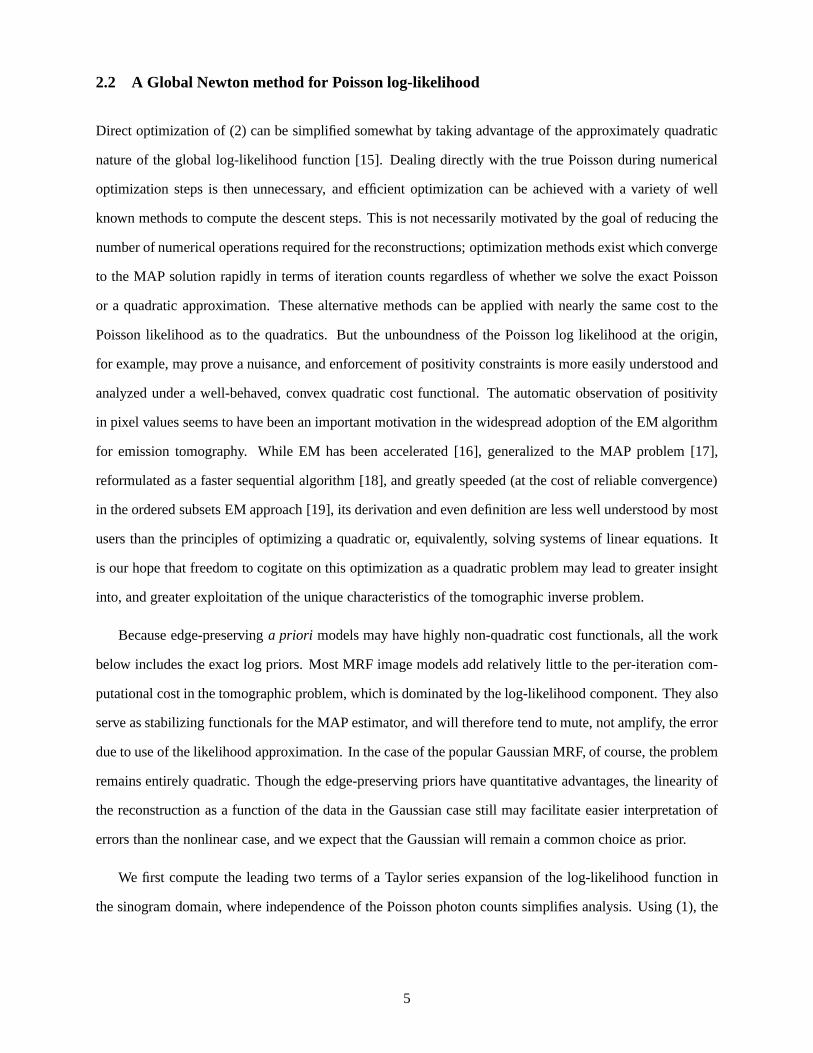
2.2 A Global Newton method for Poisson log-likelihood

Direct optimization of (2) can be simplified somewhat by taking advantage of the approximately quadratic

nature of the global log-likelihood function [15]. Dealing directly with the true Poisson during numerical

optimization steps is then unnecessary, and efficient optimization can be achieved with a variety of well

known methods to compute the descent steps. This is not necessarily motivated by the goal of reducing the

number of numerical operations required for the reconstructions; optimization methods exist which converge

to the MAP solution rapidly in terms of iteration counts regardless of whether we solve the exact Poisson

or a quadratic approximation. These alternative methods can be applied with nearly the same cost to the

Poisson likelihood as to the quadratics. But the unboundness of the Poisson log likelihood at the origin,

for example, may prove a nuisance, and enforcement of positivity constraints is more easily understood and

analyzed under a well-behaved, convex quadratic cost functional. The automatic observation of positivity

in pixel values seems to have been an important motivation in the widespread adoption of the EM algorithm

for emission tomography. While EM has been accelerated [16], generalized to the MAP problem [17],

reformulated as a faster sequential algorithm [18], and greatly speeded (at the cost of reliable convergence)

in the ordered subsets EM approach [19], its derivation and even definition are less well understood by most

users than the principles of optimizing a quadratic or, equivalently, solving systems of linear equations. It

is our hope that freedom to cogitate on this optimization as a quadratic problem may lead to greater insight

into, and greater exploitation of the unique characteristics of the tomographic inverse problem.

Because edge-preservinga priori models may have highly non-quadratic cost functionals, all the work

below includes the exact log priors. Most MRF image models add relatively little to the per-iteration com-

putational cost in the tomographic problem, which is dominated by the log-likelihood component. They also

serve as stabilizing functionals for the MAP estimator, and will therefore tend to mute, not amplify, the error

due to use of the likelihood approximation. In the case of the popular Gaussian MRF, of course, the problem

remains entirely quadratic. Though the edge-preserving priors have quantitative advantages, the linearity of

the reconstruction as a function of the data in the Gaussian case still may facilitate easier interpretation of

errors than the nonlinear case, and we expect that the Gaussian will remain a common choice as prior.

We first compute the leading two terms of a Taylor series expansion of the log-likelihood function in

the sinogram domain, where independence of the Poisson photon counts simplifies analysis. Using (1), the

5

gradient and the diagonal Hessian evaluated atp = p have entries

@ logP(Y = yjx)

@pi

����p=p

= �1 +yipi

(3)

@2 logP(Y = yjx)

@(pi)2

�����p=p

= �yi

(pi)2(4)

Different approaches may be used to take advantage of this approximation. We may evaluate it once before

any pixel update atp = y, using the raw measurement data, and keep this approximation fixed during the

convergence process [15]. In this case, an approximation to the log-likelihood is

logP(Y = yjx) � �Xi2S1

1

2yi(yi �Ai�x)

2 +Xi2S0

Ai�x+ c(y) (5)

whereS0 = fi; yi = 0g, S1 = S � S0. Since this approximation converges to the exact log likelihood asPi y

�1=2i [15], we expect the error in the approximation to be far less problematic in high-count data than

in low. The FBP image is perhaps the most practical, low-cost starting point for MAP estimation. Therefore

one may also profit from an approximation at the pointp = AxFBP .

A potentially more broadly applicable method involves updating the point of expansion after solving

the given quadratic problem, in the manner of Newton’s method in N dimensions. Newton search takes a

quadratic approximation to the objective function at each step to compute the next element of the sequential

series:

xk+1 = xk � [r2f(xk)]�1 � rf(xk) (6)

The computationally impractical inversion of the Hessian is often approximated through methods such as

preconditioning [20]. Convergence is also locally quadratic but generally not assured for non-convex ob-

jective functions, and improvements on the original idea have been developed to make Newton’s method

globally robust [21, 22]. Applying a similar methodology to the MAP estimation problem in (2), we may

use the previous estimates to globally approximate the log-likelihood as quadratic for the next image iter-

ation. The parameters of the Taylor series expansion are then evaluated from the forward projection of the

current image estimate. Due to its relation to Newton’s method in the dimension of the image, we refer to

this algorithm as global Newton (GN). Letpk be the forward projection of the image estimate obtained after

optimization on the approximate objective. The expansion pointpk is kept fixed for all pixel updates in a

stage of GN, then is updated to form the next quadratic likelihood approximation. It is computed from the

initial image (typically the FBP reconstruction) for the first iteration. Evaluating (3) and (4) atp = pk, we

6

obtain a new approximation to (1)

logP(Y = yjx) �MXi=1

yi

pki� 1

!(yi �Ai�x) +

MXi=1

�yi

2(pki )2(yi �Ai�x)

2 + c(y) (7)

To best exploit the nearly quadratic form of the log-likelihood, we seek to update only to a point where

the final GN reconstructed image will show no substantial difference from the exact MAP estimate, terminat-

ing the iterations of GN early in the sequence. In Newton’s method, the members of this series of quadratic

problems each in theory pose a computational load similar to the original estimator in (2). Therefore, the

complexity of a precise realization of GN appears to be the product of the number of necessary updates of

the global quadratic and the cost of each solution. As discussed below, however, a single iteration of an

efficient method on a global quadratic appears sufficient to warrant the next step in GN, eliminating this

additional cost. Though our implementation does not exactly solve each global quadratic before computing

a new expansion, the updates rapidly bring the minimum of the approximate objective close to the exact

MAP solution point. The projection estimatepk may then be fixed, and the solution to the final problem

form may be refined to essentially complete convergence if desired. The necessary number of updates ofpk

may be determined by off-line training appropriate to the signal-to-noise ratios typical of the given setting.

2.3 Computation of estimates via ICD

Under formulations such as (2) or (7) large-scale convex optimization must be solved. Such problems are not

difficult, but speed of convergence and simplicity of adaptation to the addition of the regularizing term and

positivity constraints in (2) are important considerations in practice. A variety of techniques may be applied

for each GN step, including all classic quadratic (constrained) optimization methods. (As mentioned above,

edge-preserving prior models may add a non-quadratic term and may also affect convergence behavior,

but typically add minor per-iteration computational cost.) In light of all the above factors, we find types

of iterative coordinate descent (ICD) well suited to the problem. The ICD algorithm is implemented by

sequentially updating each pixel of the image. With each update, the current pixel is chosen to minimize the

MAP cost function. The ICD method can be efficiently applied to the log likelihood expressions resulting

from photon limited imaging systems, is demonstrated to converge very rapidly (in our experiments typically

5-10 iterations) when initialized with the FBP reconstruction, and easily incorporates convex constraints

and non-Gaussian prior distributions. While use of approximate second derivative (Hessian) information in

this optimization has been introduced in the form of pre-conditioners for gradient and conjugate gradient

algorithms [16, 10, 11], ICD’s greedy update uses the exact local second derivative directly in one dimension.

7

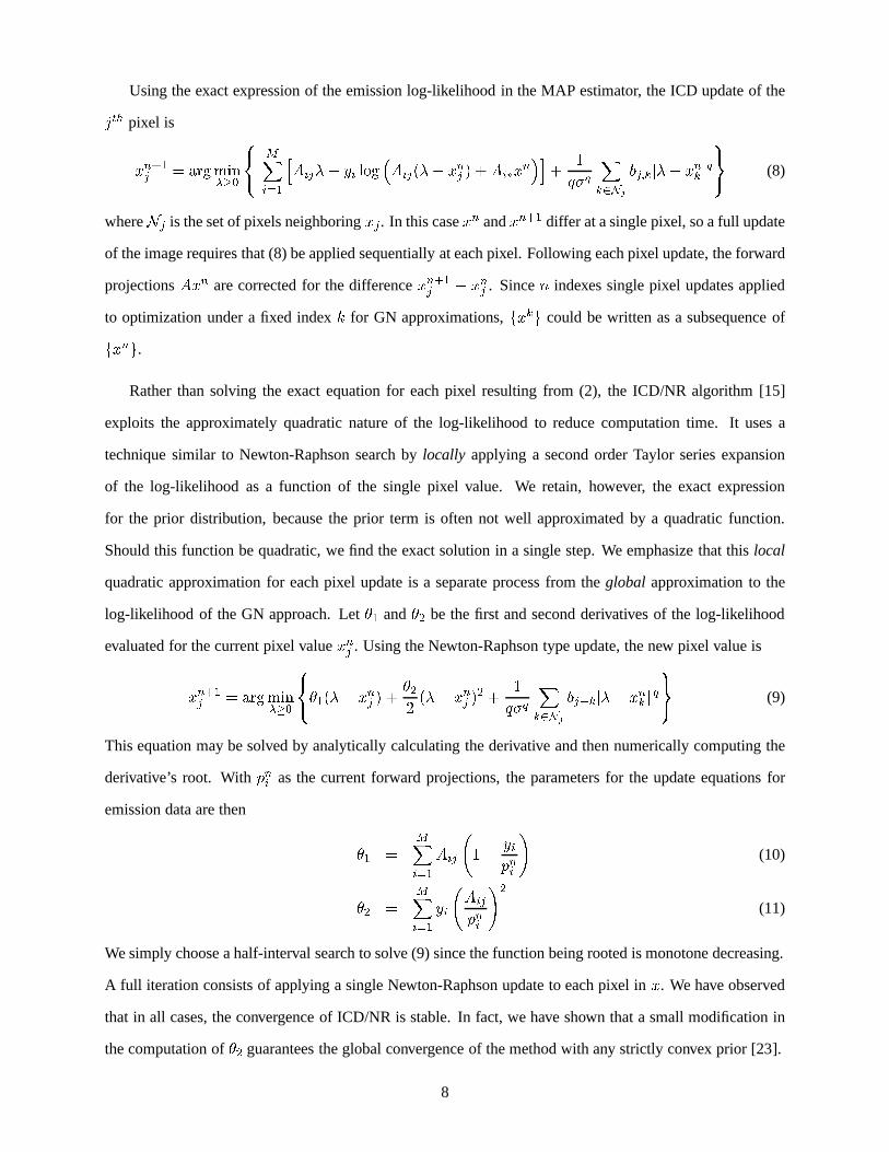
Using the exact expression of the emission log-likelihood in the MAP estimator, the ICD update of the

jth pixel is

xn+1j = argmin��0

8<:

MXi=1

hAij�� yi log

�Aij(�� xnj ) +Ai�x

n�i

+1

q�q

Xk2Nj

bj;kj�� xnk jq

9=; (8)

whereNj is the set of pixels neighboringxj. In this casexn andxn+1 differ at a single pixel, so a full update

of the image requires that (8) be applied sequentially at each pixel. Following each pixel update, the forward

projectionsAxn are corrected for the differencexn+1j � xnj . Sincen indexes single pixel updates applied

to optimization under a fixed indexk for GN approximations,fxkg could be written as a subsequence of

fxng.

Rather than solving the exact equation for each pixel resulting from (2), the ICD/NR algorithm [15]

exploits the approximately quadratic nature of the log-likelihood to reduce computation time. It uses a

technique similar to Newton-Raphson search bylocally applying a second order Taylor series expansion

of the log-likelihood as a function of the single pixel value. We retain, however, the exact expression

for the prior distribution, because the prior term is often not well approximated by a quadratic function.

Should this function be quadratic, we find the exact solution in a single step. We emphasize that thislocal

quadratic approximation for each pixel update is a separate process from theglobal approximation to the

log-likelihood of the GN approach. Let�1 and�2 be the first and second derivatives of the log-likelihood

evaluated for the current pixel valuexnj . Using the Newton-Raphson type update, the new pixel value is

xn+1j = argmin��0

8<:�1(�� xnj ) +

�22(�� xnj )

2 +1

q�q

Xk2Nj

bj�kj�� xnk jq

9=; (9)

This equation may be solved by analytically calculating the derivative and then numerically computing the

derivative’s root. Withpni as the current forward projections, the parameters for the update equations for

emission data are then

�1 =MXi=1

Aij

1�

yipni

!(10)

�2 =MXi=1

yi

Aij

pni

!2

(11)

We simply choose a half-interval search to solve (9) since the function being rooted is monotone decreasing.

A full iteration consists of applying a single Newton-Raphson update to each pixel inx. We have observed

that in all cases, the convergence of ICD/NR is stable. In fact, we have shown that a small modification in

the computation of�2 guarantees the global convergence of the method with any strictly convex prior [23].

8

Using an approximation such as GN, with (7) in place of the exact Poisson log-likelihood in equation

(2), the computation of the update of thejth pixel is realized as in (9) with new expressions for�1 and�2

�1 =MXi=1

Aij

1 +

yipki

pnipki

� 2

!!(12)

�2 =MXi=1

yi

Aij

pki

!2

(13)

We label this form of coordinate descent ICD/GN. Updating this quadratic approximation at each pixel

(replacingpki with pni ) would reduce to the exact solution case of (10) and (11), which means that ICD/GN

reduces to ICD/NR in this case. In the present ICD/GN, we keep this approximation fixed for a whole

iteration through the image before updating it. Powell [20] proved the global convergence of an algorithm

of this type when the Hessian is positive definite everywhere in an open convex set. This corresponds

geometrically to strict convexity as in our case, and we have observed stable convergence in all experiments.

Computation time is dominated by the multiplies and divides required to compute�1 and�2. Both in

ICD/NR of Section 2.3, and in equations (12) and (13), notingM0 the number of non-zero projections, this

results in4M0N operations per full image update with the appropriate storage ofyi=(pki )

2 andpn. There-

fore, ICD/GN and ICD/NR require approximately the same time for one iteration, including re-evaluation of

the expansion point. If we terminate these evaluations,�2 is constant. In addition, both are also equivalent

in terms of the number of indexings through the projection matrixA, each requiring two, and the use of the

approximation is not computationally more expensive.

The optimal scan pattern for the sequential pixel updates of the greedy ICD algorithm is not obvious,

since nothing in the information carried by the sinogram dictates the best order in which the image pixels

should be visited. The order of pixel updates affects convergence speed, and therefore may warrant study to

determine the best method. Lexicographic scans which iterate in horizontal, then vertical coordinates every

other iteration have advantages analytically [24], but in our experiments here, simple repeated horizontal

scans performed slightly better. Improved convergence speed seems also to be achieved using a random scan

pattern [25]. Unless otherwise noted, all results presented here are from random patterns which visit each

pixel once per scan. We present below comparisons in objective convergence between a simple lexicographic

pattern and a random pattern.

9

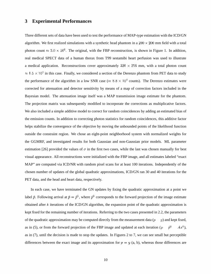
3 Experimental Performances

Three different sets of data have been used to test the performance of MAP-type estimation with the ICD/GN

algorithm. We first realized simulations with a synthetic head phantom in a200� 200 mm field with a total

photon count� 3:0 � 106. The original, with the FBP reconstruction, is shown in Figure 1. In addition,

real medical SPECT data of a human thorax from T99 sestamibi heart perfusion was used to illustrate

a medical application. Reconstructions cover approximately320 � 256 mm, with a total photon count

� 1:5 � 105 in this case. Finally, we considered a section of the Derenzo phantom from PET data to study

the performance of the algorithm in a low SNR case (� 8:8 � 104 counts). The Derenzo estimates were

corrected for attenuation and detector sensitivity by means of a map of correction factors included in the

Bayesian model. The attenuation image itself was a MAP transmission image estimate for the phantom.

The projection matrix was subsequently modified to incorporate the corrections as multiplicative factors.

We also included a simple additive model to correct for random coincidences by adding an estimated bias of

the emission counts. In addition to correcting photon statistics for random coincidences, this additive factor

helps stabilize the convergence of the objective by moving the unbounded points of the likelihood function

outside the constraint region. We chose an eight-point neighborhood system with normalized weights for

the GGMRF, and investigated results for both Gaussian and non-Gaussian prior models. ML parameter

estimation [26] provided the values of� in the first two cases, while the last was chosen manually for best

visual appearance. All reconstructions were initialized with the FBP image, and all estimates labeled “exact

MAP” are computed via ICD/NR with random pixel scans for at least 100 iterations. Independently of the

chosen number of updates of the global quadratic approximations, ICD/GN ran 30 and 40 iterations for the

PET data, and the head and heart data, respectively.

In each case, we have terminated the GN updates by fixing the quadratic approximation at a point we

label �p. Following arrival at�p = pk, wherepk corresponds to the forward projection of the image estimate

obtained afterk iterations of the ICD/GN algorithm, the expansion point of the quadratic approximation is

kept fixed for the remaining number of iterations. Referring to the two cases presented in 2.2, the parameters

of the quadratic approximation may be computed directly from the measurement data (�p = y) and kept fixed,

as in (5), or from the forward projection of the FBP image and updated at each iteration (�p = pk = Axk),

as in (7), until the decision is made to stop the updates. In Figures 2 to 7, we can see small but perceptible

differences between the exact image and its approximation for�p = y (a, b), whereas those differences are

10

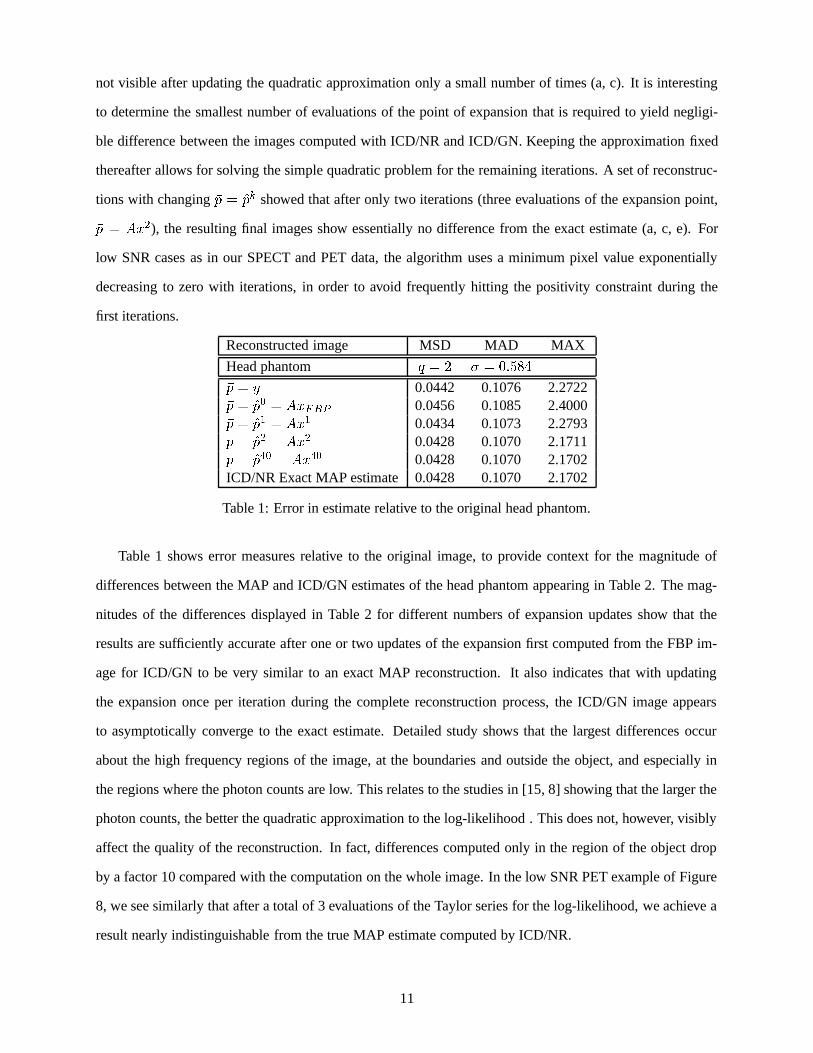
not visible after updating the quadratic approximation only a small number of times (a, c). It is interesting

to determine the smallest number of evaluations of the point of expansion that is required to yield negligi-

ble difference between the images computed with ICD/NR and ICD/GN. Keeping the approximation fixed

thereafter allows for solving the simple quadratic problem for the remaining iterations. A set of reconstruc-

tions with changing�p = pk showed that after only two iterations (three evaluations of the expansion point,

�p = Ax2), the resulting final images show essentially no difference from the exact estimate (a, c, e). For

low SNR cases as in our SPECT and PET data, the algorithm uses a minimum pixel value exponentially

decreasing to zero with iterations, in order to avoid frequently hitting the positivity constraint during the

first iterations.

Reconstructed image MSD MAD MAX

Head phantom q = 2 � = 0:584

�p = y 0.0442 0.1076 2.2722�p = p0 = AxFBP 0.0456 0.1085 2.4000�p = p1 = Ax1 0.0434 0.1073 2.2793�p = p2 = Ax2 0.0428 0.1070 2.1711�p = p40 = Ax40 0.0428 0.1070 2.1702ICD/NR Exact MAP estimate 0.0428 0.1070 2.1702

Table 1: Error in estimate relative to the original head phantom.

Table 1 shows error measures relative to the original image, to provide context for the magnitude of

differences between the MAP and ICD/GN estimates of the head phantom appearing in Table 2. The mag-

nitudes of the differences displayed in Table 2 for different numbers of expansion updates show that the

results are sufficiently accurate after one or two updates of the expansion first computed from the FBP im-

age for ICD/GN to be very similar to an exact MAP reconstruction. It also indicates that with updating

the expansion once per iteration during the complete reconstruction process, the ICD/GN image appears

to asymptotically converge to the exact estimate. Detailed study shows that the largest differences occur

about the high frequency regions of the image, at the boundaries and outside the object, and especially in

the regions where the photon counts are low. This relates to the studies in [15, 8] showing that the larger the

photon counts, the better the quadratic approximation to the log-likelihood . This does not, however, visibly

affect the quality of the reconstruction. In fact, differences computed only in the region of the object drop

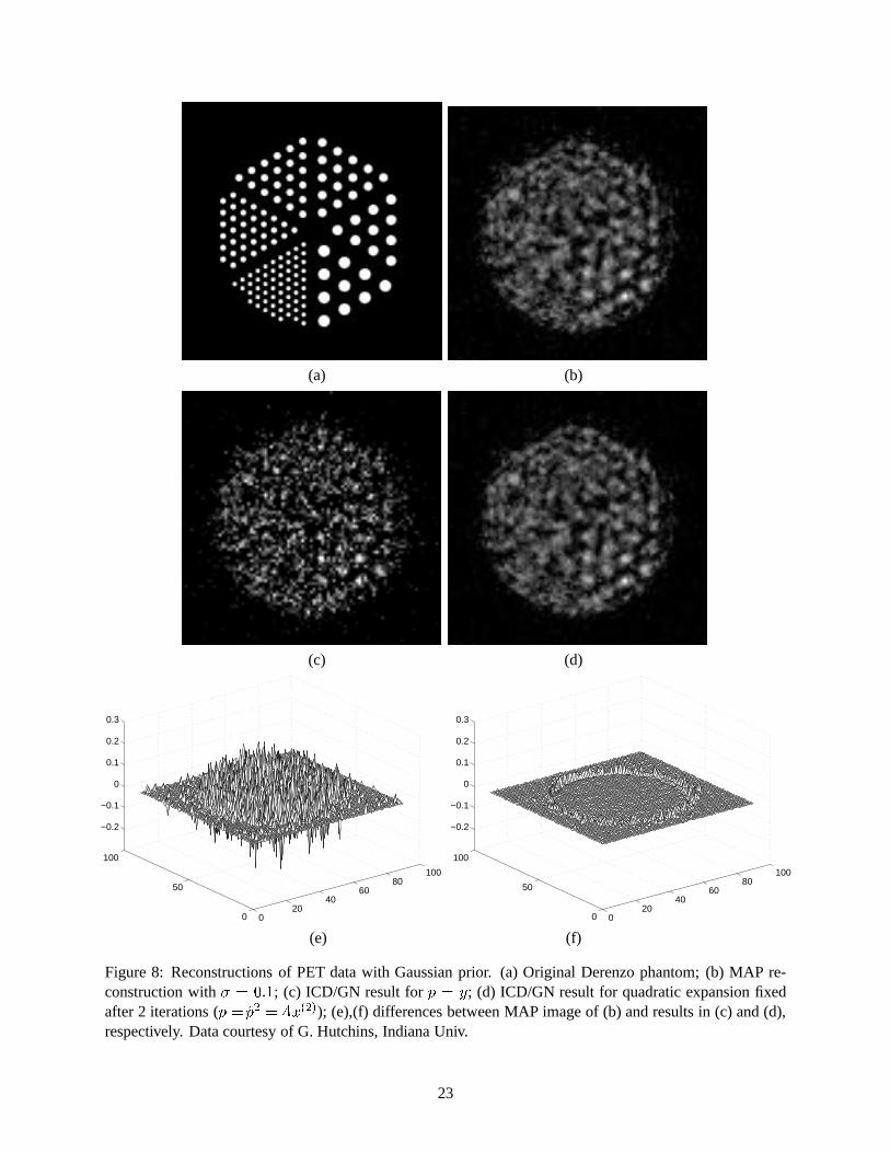
by a factor 10 compared with the computation on the whole image. In the low SNR PET example of Figure

8, we see similarly that after a total of 3 evaluations of the Taylor series for the log-likelihood, we achieve a

result nearly indistinguishable from the true MAP estimate computed by ICD/NR.

11

Expansion point MSD MAD MAX

Head Phantom q = 2 � = 0:584

�p = y 4:663 � 10�4 8:413 � 10�3 5:160 � 10�1

�p = p0 = AxFBP 8:393 � 10�4 6:00 � 10�3 5:160 � 10�1

�p = p1 = Ax1 1:325 � 10�4 2:208 � 10�4 2:327 � 10�1

�p = p2 = Ax2 1:428 � 10�7 6:685 � 10�5 1:45 � 10�2

SPECT data q = 2 � = 0:0283

�p = y 3:969 � 10�5 2:572 � 10�3 5:88 � 10�2

�p = p0 = AxFBP 2:165 � 10�5 1:813 � 10�3 4:17 � 10�2

�p = p1 = Ax1 3:772 � 10�6 6:358 � 10�4 2:43 � 10�2

�p = p2 = Ax2 5:319 � 10�7 2:165 � 10�4 1:18 � 10�2

Derenzo PET data q = 2 � = 0:10

�p = y 4:468 � 10�4 6:145 � 10�3 2:736 � 10�1

�p = p0 = AxFBP 9:840 � 10�5 3:105 � 10�3 1:510 � 10�1

�p = p1 = Ax1 2:490 � 10�5 1:369 � 10�3 1:024 � 10�1

�p = p2 = Ax2 5:619 � 10�6 4:919 � 10�4 5:87 � 10�2

Table 2: Difference measurements between MAP and ICD/GN images for varying numbers of evaluationsof the global quadratic approximation

Interestingly, the quantitative results indicate that fixing the quadratic expansion from the forward pro-

jection of the FBP image is not necessarily better than using the raw sinogram with�p = y. The high

frequency noise present in the original sinogram is spread over the entire image by the FBP reconstruction,

and may therefore be spread over the entire sinogram resulting from the forward projection of the FBP

image. In contrast, the vectory remains as the standard for the estimate’s fidelity to the data throughout

GN updates. Therefore, it is plausible that the minimum of the resulting GN quadratic approximation at

�p = p0 = AxFBP may be farther from the MAP estimate than the one made at�p = y. The use of the

FBP image as starting point for ICD/GN has several motivations. The FBP image is good first estimate of

image densities which is quickly computed. In addition, the ICD algorithm is very efficient in converging

the high frequencies in the image, while somewhat slower for low frequencies; the FBP image offers low

frequency components already near their optimal value. This makes the FBP image a good starting point

for most iterative estimation algorithms. However, it is quite conceivable that in some instances of GN, one

might use stillx0 = xFBP with p0 = y in place ofAxFBP .

The convergence plots of Figure 9 correspond to the above results. They were obtained for Gaussian

priors and used a regular scan pattern in horizontal coordinates first. The plots are similar in the case

of non-Gaussian priors. For the head and the Derenzo phantoms, ICD/GN exhibits the same behavior as

ICD/NR, indicating experimentally that the global quadratic approximations do not affect the convergence

12

properties of the ICD algorithm. Whatever choice is made for fixing the quadratic approximation, the

objective function converges quickly (typically about five iterations). However, it appears in the SPECT

data plot that if we evaluate the quadratic approximation at�p = y and keep it fixed thereafter (“0” plots),

the limiting a posterioriprobability is significantly different from the exact MAP objective. Updating the

quadratic approximation only once after its first evaluation from the FBP image leaves only small differences

in the objective values of ICD/GN and ICD/NR.

With the exception of the plots in Figure 9, all the figures presented thus far result from ICD pixel

updates in random order. The patterns analyzed in [24] were regular, by lines or by columns, but recent

results have shown a potential for improvement in convergence speed with these randomly ordered scans

[25]. Figure 10 presents the improvement in convergence speed that a random update pattern offers over a

regular lexicographic scan in the case of the Derenzo phantom. A simple linear congruential random number

generator guarantees that each pixel in the image is visited once and only once per iteration. The gain here

is significant, since after only two iterations the objective has almost converged when the random scan is

used, whereas six iterations are necessary when using the lexicographic scan. In addition, it is interesting

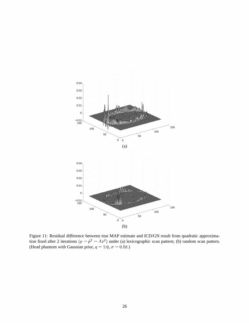
to study the influence of the scan pattern on the ICD/GN results. Figures 10 and 11 compare the image

estimates for�p = p2 when using the lexicographic or random update pattern. The magnitude plots show

that the random pattern eliminates some of the differences between the GN estimate and the exact MAP

image. With a sequential update of the pixels, the first pixels in the image tend to be overcorrected since

the objective function is greedily optimized at each step. A lexicographic scan, such as in 10 (b) and 11

(a), therefore creates more low frequency artifacts in the image and tends to concentrate those pixels on

whichever side of the object is updated first, whereas a random pattern scatters them. The differences in

the above figures appear in fact to be the superposition of both the overcorrection discussed above, and the

low frequency components which take longer to converge with ICD. Thus the random pattern may offer

faster convergence of both the global approximations of GN, and the sweeps of the image under ICD. A

potentially interesting variation on the random update would involve a non-uniform spatial distribution of

updates dependent on the current image estimate.

These results suggest that any algorithm which converges rapidly for the first few iterations might

quickly supply a final global quadratic likelihood approximation, which could then be attacked by any

numerical algorithm well suited to quadratic objectives. An initially quite rapid, though non-convergent,

form of EM which cycles among subsets of data, known as ordered subsets EM (OSEM) [19], might be

13

used for the initial estimates, and another, e.g. conjugate gradient or ICD, might be applied to convergence

of the resulting fixed quadratic problem [25].

4 Conclusion

In Bayesian tomography, the substitution of an approximation to the log-likelihood function allows simpler

optimization of the MAP objective without computation under the Poisson model. After only a few updates

of the global quadratic, a coordinate descent method rapidly converges to an estimate nearly indistinguish-

able from the exact MAP estimate. For emission tomographic problems of medium to high signal-to-noise

ratios, our results suggest that viewing the log-likelihood as quadratic may be adequate for any visual in-

terpretations, and would open the problem to researchers and practitioners more accustomed to quadratic

constrained optimization than photon-limited image reconstruction. Even in low-count problems, it appears

that little appreciable quality would be sacrificed in optimizing a quadratic log-likelihood approximation

fixed very early in the process. These claims all assume the use of relatively rapidly converging techniques

for the first few iterations. Further research will evaluate differences between ICD and OSEM for the initial

stages.

References

[1] S. Geman and D. McClure, “Bayesian images analysis: An application to single photon emission tomography,”in Proc. Statist. Comput. sect. Amer. Stat. Assoc., pp. 12–18, (Washington, DC), 1985.

[2] L. Shepp and Y. Vardi, “Maximum likelihood reconstruction for emission tomography,”IEEE Trans. on MedicalImagingMI-1 , pp. 113–122, October 1982.

[3] R. Gordon and G. Herman, “Three-dimensional reconstruction from projections: A review of algorithms,” inInternational Review of Cytology, G. Bourne and J. Danielli, eds., vol. 38, pp. 111–151, Academic Press, NewYork, 1974.

[4] G. T. Herman and A. Lent, “A computer implementation of a Bayesian analysis of image reconstruction,”Infor-mation and Control31, pp. 364–384, 1976.

[5] E. Artzy, T. Elfving, and G. T. Herman, “Quadratic optimization for image reconstruction,”Computer Graphicsand Image Processing11, pp. 242–261, 1979.

[6] S. L. Wood and M. Morf, “A fast implementation of a minimum variance estimator for computerized tomographyimage reconstruction,”IEEE Trans. on Biomedical EngineeringBME-28, pp. 56–68, February 1981.

[7] B. Tsui, E. Frey, and G. Gullberg, “Comparison between ML-EM and WLS-CG algorithms for SPECT imagereconstruction,”IEEE Trans. on Nuclear Science38, pp. 1766–1772, December 1991.

[8] J. Fessler, “Hybrid poisson/polynomial objective functions for tomographic image reconstruction from transmis-sion scans,”IEEE Trans. on Image Processing4, pp. 1439–1450, October 1995.

[9] P. Koulibaly,Regularisation et Corrections Physiques en Tomographie d’Emission, Ph.D. Thesis, Univ. of Nice-Sophia Antipolis, France, Oct. 1996.

14

[10] N. Clinthorne, T. Pan, P.-C. Chiao, W. Rogers, and J. Stamos, “Preconditioning methods for improved conver-gence rates in iterative reconstruction,”IEEE Trans. on Medical Imaging12, pp. 78–83, March 1993.

[11] E. �U . Mumcuo�glu, R. Leahy, S. R. Cherry, and Z. Zhou, “Fast gradient-based methods for Bayesian reconstruc-tion of transmission and emission pet images,”IEEE Trans. on Medical Imaging13, pp. 687–701, December1994.

[12] D. Snyder and M. Miller, “The use of sieves to stabilize images produced with the EM algorithm for emissiontomography,”IEEE Trans. Nucl. Sci.NS-32, pp. 3864–3871, Oct. 1985.

[13] J. Llacer and E. Veklerov, “Feasible images and practical stopping rules for iterative algorithms in emissiontomography,”IEEE Trans. on Medical Imaging8, pp. 186–193, 1989.

[14] C. A. Bouman and K. Sauer, “A generalized Gaussian image model for edge-preserving map estimation,”IEEETrans. on Image Processing2, pp. 296–310, July 1993.

[15] C. A. Bouman and K. Sauer, “A unified approach to statistical tomography using coordinate descent optimiza-tion,” IEEE Trans. on Image Processing5, pp. 480–492, March 1996.

[16] L. Kaufman, “Implementing and accelerating the EM algorithm for positron emission tomography,”IEEE Trans.on Medical ImagingMI-6 (1), pp. 37–51, 1987.

[17] A. D. Pierro, “A modified expectation maximization algorithm for penalized likelihood estimation in emissiontomography,”IEEE Trans. on Medical Imaging14(1), pp. 132–137, 1995.

[18] J. Fessler and A. Hero, “Complete data spaces and generalized em algorithms,” inProc. of IEEE Int’l Conf. onAcoust., Speech and Sig. Proc., vol. IV, pp. 1–4, (Minneapolis, Minnesota), April 27-30 1993.

[19] H. Hudson and R. Larkin, “Accelerated image reconstruction using ordered subsets of projection data,”IEEETrans. on Medical Imaging13, pp. 601–609, December 1994.

[20] J. Dennis and R. Schnabel,Numerical Methods for Unconstrained Optimization and Nonlinear Equations,Prentice-Hall, Englewood Cliffs, NJ, 1983.

[21] D. Luenberger,Introduction to Linear and Nonlinear Programming, Addison-Wesley, Reading, MA, 1973.

[22] S. Jacoby, J. Kowalik, and J. Pizzo,Iterative Methods for Nonlinear Optimization Problems, Prentice-Hall,Englewood Cliffs, NJ, 1972.

[23] S. Saquib, J. Zheng, C. A. Bouman, and K. D. Sauer, “Provably convergent coordinate descent in statistical to-mographic reconstruction,” inProc. of IEEE Int’l Conf. on Image Proc., vol. II, pp. 741–744, (Lausanne Switzer-land), September 16-19 1996.

[24] K. Sauer and C. A. Bouman, “A local update strategy for iterative reconstruction from projections,”IEEE Trans.on Signal Processing41, February 1993.

[25] J. Bowsher, M. Smith, J. Peter, and R. Jaszczak, “A comparison of OSEM and ICD for iterative reconstructionof SPECT brain images,”Journal of Nuclear Medicine39, p. 79P, 1998.

[26] C. A. Bouman and K. Sauer, “Maximum likelihood scale estimation for a class of Markov random fields,” inProc. of IEEE Int’l Conf. on Acoust., Speech and Sig. Proc., vol. 5, pp. 537–540, (Adelaide, South Australia),April 19-22 1994.

15

(a)

(b)

Figure 1: Head phantom used for reconstruction comparisons. (a) Original phantom; (b) FBP reconstruction.

16

(a)

(b)

(c)

Figure 2: Reconstructions of head phantom with Gaussian prior. (a) Exact MAP image, Gaussian prior and� = 0:58; (b) Estimate with quadratic log-likelihood approximation fixed at�p = y; (c) ICD/GN result forquadratic approximation fixed after 2 iterations(�p = p2 =Ax2).

17

(a) 020

4060

80100

120140

0

50

100

150−1.5

−1

−0.5

0

0.5

1

1.5

2

2.5

(b) 0

50

100

0

50

100

−0.1

0

0.1

0.2

0.3

0.4

0.5

(c) 0

50

100

0

50

100

−0.1

0

0.1

0.2

0.3

0.4

0.5

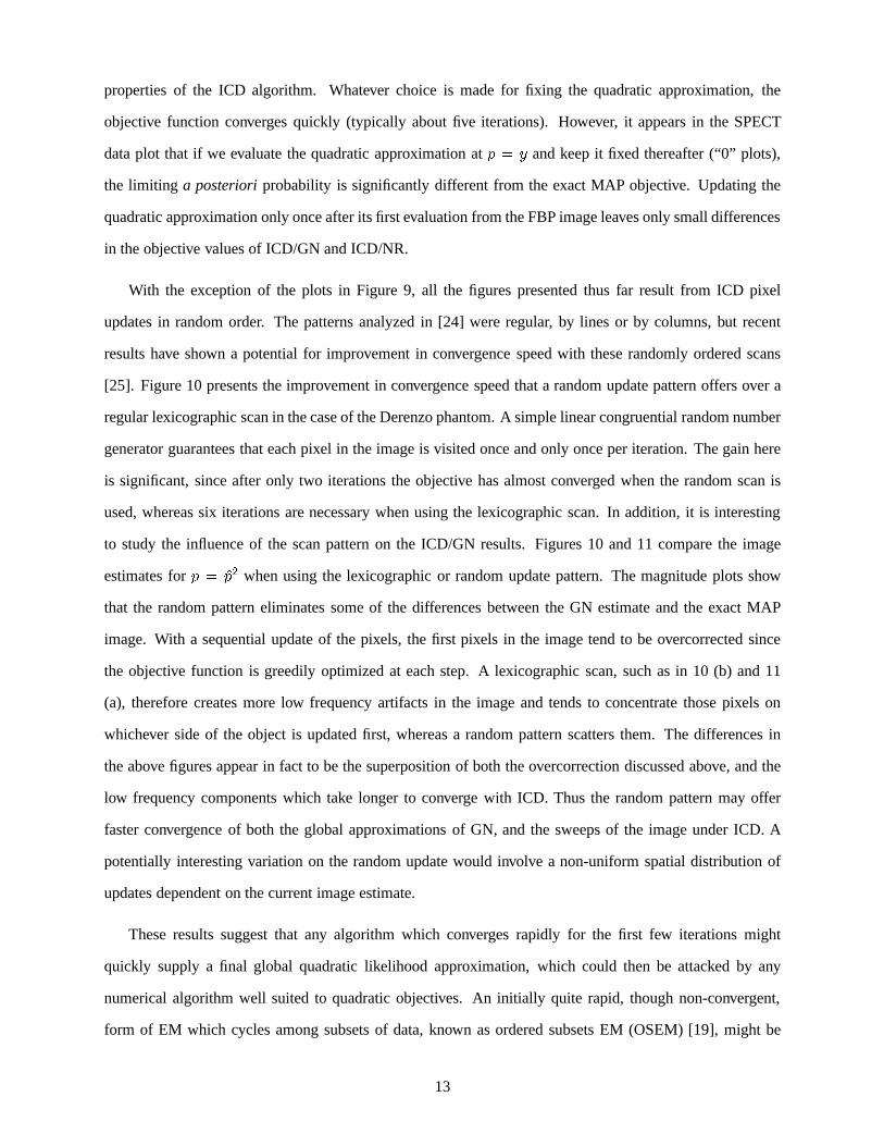
Figure 3: MAP reconstruction with GGMRF, Gaussian prior(q = 2:0) and� = 0:58. (a) Error betweenoriginal phantom and MAP reconstruction; (b) difference between MAP and estimate using quadratic fixedat �p = y; (c) difference between MAP and estimate using quadratic fixed at�p = p2 =Ax2.

18

(a)

(b)

(c)

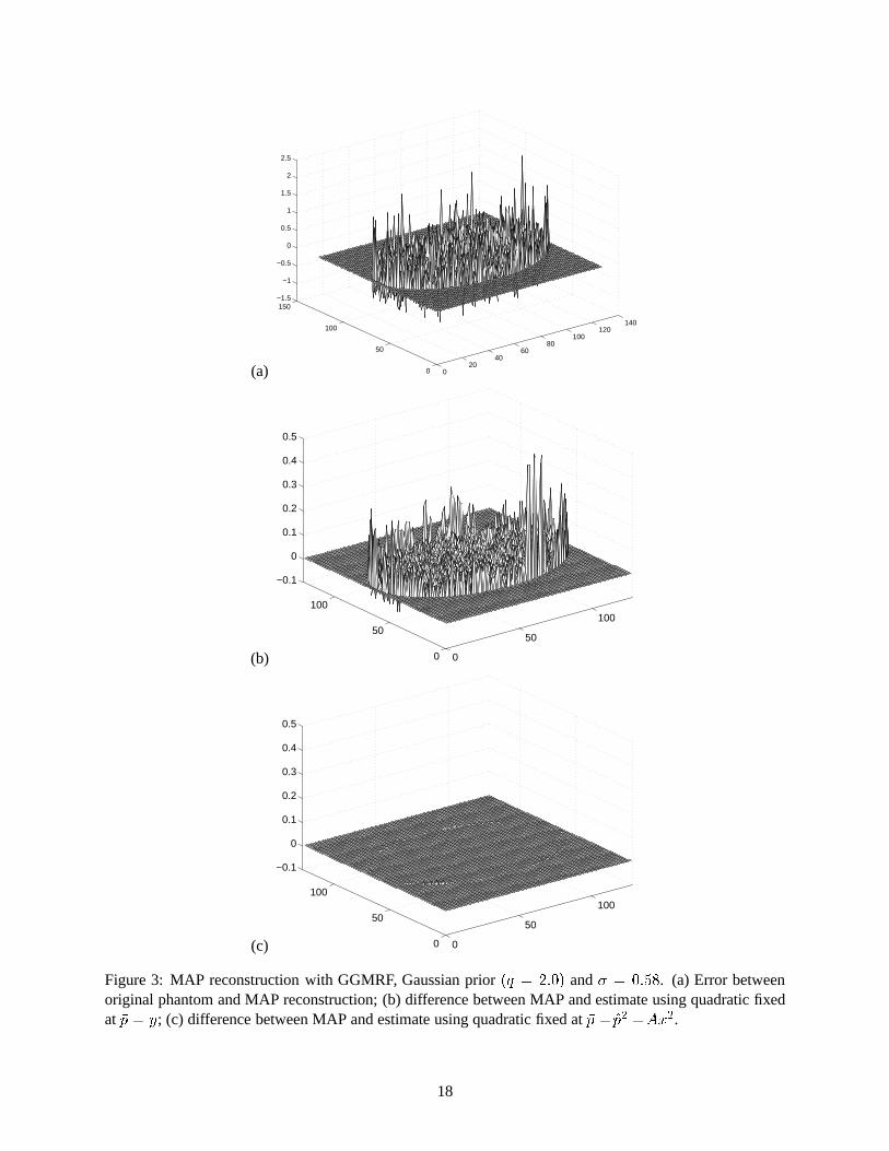
Figure 4: Reconstructions of a head phantom with non-Gaussian GGMRF prior(q = 1:1), � = 0:25. (a)Exact MAP image; (b) Estimate with fixed quadratic approximation evaluated at�p = y; (c) ICD/GN resultwith fixed approximation after two iterations(�p = p2 =Ax2).

19

(a) 0

50

100

0

50

100

−2

−1

0

1

2

3

(b) 0

50

100

0

50

100

0

0.2

0.4

0.6

0.8

1

(c) 0

50

100

0

50

100

0

0.2

0.4

0.6

0.8

1

Figure 5: MAP reconstruction with GGMRF,q = 1:1, � = 0:25. (a) Error between original phantom andMAP reconstruction; (b) difference between MAP and estimate using quadratic at�p = y; (c) differencebetween MAP and estimate from quadratic using�p = p2 =Ax2.

20

(a)

(b) (c)

020

4060

80

0

20

40

60

80−0.02

0

0.02

0.04

0.06

020

4060

80

0

20

40

60

80−0.02

0

0.02

0.04

0.06

(d) (e)

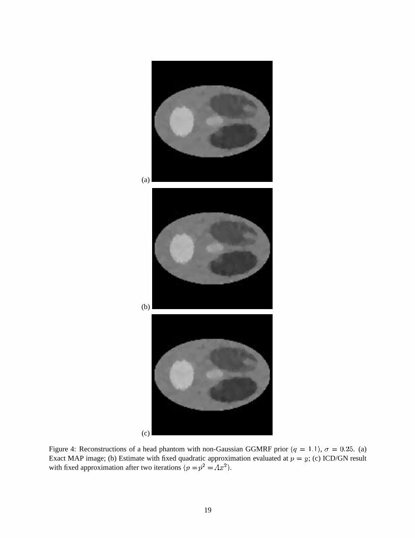
Figure 6: Reconstructions of SPECT data with Gaussian prior and� = 0:028. (a) Exact MAP image; (b)Estimate using quadratic at�p = y; (c) ICD/GN result for 2 updates of the expansion point(�p = p2 =Ax2); (d)(e) differences between (a) and (b),(c), respectively. Data courtesy of T.S. Pan and M. King, Univ. ofMass.

21

(a)

(b) (c)

020

4060

80

0

20

40

60

80−0.05

0

0.05

0.1

020

4060

80

0

20

40

60

80−0.05

0

0.05

0.1

(d) (e)

Figure 7: Reconstructions of SPECT data with non-Gaussian GGMRF prior,q = 1:1 and� = 0:017. (a)Exact MAP image; (b) Estimate using quadratic at�p = y; (c) ICD/GN result for 2 updates of the expansionpoint (�p = p2 =Ax2); (d),(e) differences between (a) and (b),(c), respectively. Data courtesy of T.S. Panand M. King, Univ. of Mass.

22

(a) (b)

(c) (d)

020

4060

80100

0

50

100

−0.2

−0.1

0

0.1

0.2

0.3

020

4060

80100

0

50

100

−0.2

−0.1

0

0.1

0.2

0.3

(e) (f)

Figure 8: Reconstructions of PET data with Gaussian prior. (a) Original Derenzo phantom; (b) MAP re-construction with� = 0:1; (c) ICD/GN result for�p = y; (d) ICD/GN result for quadratic expansion fixedafter 2 iterations (�p = p2 =Ax(2)); (e),(f) differences between MAP image of (b) and results in (c) and (d),respectively. Data courtesy of G. Hutchins, Indiana Univ.

23

0 5 10 15 20 25 30 35 40942.5

943

943.5

944

944.5

945

945.5

Iterations

log

a po

ster

iori

prob

abili

ty

ICD/NR4010510

(a)

0 5 10 15 20 25 30 35 4016.6

16.8

17

17.2

17.4

17.6

17.8

Iterations

log

a po

ster

iori

prob

abili

ty

ICD/NR520

(b)

0 5 10 15 20 25 30−3

−2.5

−2

−1.5

−1

−0.5

0

Iterations

log

a po

ster

iori

prob

abili

ty

ICD/NRICD/GN 10ICD/GN 5ICD/GN 3ICD/GN 2

(c)

Figure 9: Convergence of objectivevs iterations for (a) the head phantom, (b) the SPECT data, and (c)the PET data, for various number of evaluations of the expansion point. Convergence plots obtained fromordered pixel updates in horizontal coordinates first in ICD. ”0” indicates�p = y, ”1” indicates �p = p0 =AxFBP , ”2” indicates�p = p1 =Ax1, etc.

24

0 5 10 15−2.5

−2

−1.5

−1

−0.5

0

0.5

Iterations

Log

a po

ster

iori

prob

abili

ty

RegularRandom

(a)

020

4060

80100

0

50

100−0.05

0

0.05

0.1

0.15

0.2

(b)

020

4060

80100

0

50

100−0.05

0

0.05

0.1

0.15

0.2

(c)

Figure 10: Difference in convergence behavior between lexicographic scan in horizontal coordinates first,and randomly ordered pixel updates in ICD, for the Derenzo phantom with Gaussian prior. (a) Convergenceof log a posterioriprobability in both cases. Residual difference between true MAP estimate and result fromquadratic approximation fixed after 2 iterations(�p = p2 =Ax2) under (b) regular scan pattern; (c) randomscan pattern.

25

0

50

100

150

0

50

100

150−0.01

0

0.01

0.02

0.03

0.04

(a)

0

50

100

150

0

50

100

150−0.01

0

0.01

0.02

0.03

0.04

(b)

Figure 11: Residual difference between true MAP estimate and ICD/GN result from quadratic approxima-tion fixed after 2 iterations(�p = p2 =Ax2) under (a) lexicographic scan pattern; (b) random scan pattern.(Head phantom with Gaussian prior,q = 2:0, � = 0:58.)

26