nice guys finish last: are people with higher tax morale ...ftp.iza.org/dp6275.pdf · nice guys...
TRANSCRIPT

DI
SC
US
SI
ON
P
AP
ER
S
ER
IE
S
Forschungsinstitut zur Zukunft der ArbeitInstitute for the Study of Labor
Nice Guys Finish Last:Are People with Higher Tax Morale Taxed More Heavily?
IZA DP No. 6275
January 2012
Philipp DoerrenbergDenvil DuncanClemens FuestAndreas Peichl
Nice Guys Finish Last: Are People with Higher Tax Morale
Taxed More Heavily?
Philipp Doerrenberg CGS, University of Cologne and IZA
Denvil Duncan
Indiana University and IZA
Clemens Fuest University of Oxford, University of Cologne, CESifo and IZA
Andreas Peichl
IZA, University of Cologne, ISER and CESifo
Discussion Paper No. 6275 January 2012
IZA
P.O. Box 7240 53072 Bonn
Germany
Phone: +49-228-3894-0 Fax: +49-228-3894-180
E-mail: [email protected]
Any opinions expressed here are those of the author(s) and not those of IZA. Research published in this series may include views on policy, but the institute itself takes no institutional policy positions. The Institute for the Study of Labor (IZA) in Bonn is a local and virtual international research center and a place of communication between science, politics and business. IZA is an independent nonprofit organization supported by Deutsche Post Foundation. The center is associated with the University of Bonn and offers a stimulating research environment through its international network, workshops and conferences, data service, project support, research visits and doctoral program. IZA engages in (i) original and internationally competitive research in all fields of labor economics, (ii) development of policy concepts, and (iii) dissemination of research results and concepts to the interested public. IZA Discussion Papers often represent preliminary work and are circulated to encourage discussion. Citation of such a paper should account for its provisional character. A revised version may be available directly from the author.

IZA Discussion Paper No. 6275 January 2012
ABSTRACT
Nice Guys Finish Last: Are People with Higher Tax Morale Taxed More Heavily?*
This paper is the first to provide evidence of efficient taxation of groups with heterogeneous levels of ‘tax morale’. We set up an optimal income tax model where high tax morale implies a high subjective cost of evading taxes. The model predicts that ‘nice guys finish last’: groups with higher tax morale will be taxed more heavily, simply because taxing them is less costly. Based on unique cross-country micro data and an IV approach to rule out reverse causality, we find empirical support for this hypothesis. Income groups with high tax morale systematically face higher average and marginal tax rates. JEL Classification: H2, H3, D7 Keywords: tax morale, tax compliance, optimal taxation, political economy Corresponding author: Andreas Peichl IZA P.O. Box 7240 53072 Bonn Germany E-mail: [email protected]
* Andreas Peichl is grateful for financial support from Deutsche Forschungsgemeinschaft DFG (PE1675). We are grateful to Klara Sabirianova-Peter for providing us with tax rate data from the World Tax Indicators. We would like to thank Oleg Badunenko, Felix Bierbrauer, Dan Hamermesh, Bradley Heim, Stephen Jenkins, Jorge Luis Martinez, Nico Pestel, Andrew Oswald, Salmai Qari, Justin Ross, Sebastian Siegloch, Andràs Simonovits, Caroline Weber, Jeff Wooldridge and participants of the IIPF 2011 (Ann Arbor), shadow2011 (Münster) and CESifo Political Economy (Dresden) conferences, as well as seminars in Bonn, Cologne, and Uppsala for helpful comments and suggestions. The usual disclaimer applies.
1 Introduction
Tax morale1—the intrinsic motivation to honestly pay taxes—is widely seen as ad-
vantageous for an economy because it reduces the cost of financing the public sector.
Therefore, a large part of the academic and political debate focuses on the impact
of institutions and policies on tax morale and on ways of improving it. This paper
takes a different perspective and explores whether differences in tax morale across
different groups of taxpayers within and across countries affect the tax burden im-
posed on these groups. Our main hypothesis is that groups with a high level of
tax morale are taxed more heavily because taxing them creates smaller distortions.
Using unique cross-country micro data and an Instrumental Variable (IV) approach,
we provide robust evidence supporting our hypothesis.
The theoretical basis of our approach is straightforward. We start from the
observation that different groups of individuals within one country as well as across
countries can have different levels of tax morale. If the absolute amount of tax paid
by a particular group of taxpayers is given, a high level of tax morale will imply that
the tax base is large, so that tax rates can be low. This is advantageous because tax
distortions of economic activity are smaller and tax enforcement and administration
costs are lower than in cases where tax morale is low. It pays to have a high level
of tax morale in such a world. However, if the tax revenue raised from particular
groups of taxpayers is not given, groups with a high level of tax morale may end
up paying higher taxes than groups with low tax morale. The reason is that a high
level of tax morale reduces the cost of taxation, since groups with low tax morale
respond to increases in taxation by evading more, relative to high morale groups.
We set up a simple model of optimal taxation, where the government maxi-
mizes an objective function in which each group of taxpayers has a given weight.
The weight may depend on income, political influence, or other factors, but is un-
related to tax morale. Tax morale is introduced by assuming that different groups
of taxpayers face different subjective costs of evading taxes. In this model, the
government will systematically impose higher tax rates on groups with higher tax
morale because taxing them causes smaller distortions. Our theoretical analysis
thus yields the hypothesis that ‘nice guys finish last’: groups with high tax morale
are ‘punished’ through the tax system because governments tax these groups more
heavily.
We test our hypothesis using data from the World Value Survey (WVS), the
1The term ‘tax morale’ might be misleading and ‘tax honesty’ or ‘tax ethics’ might be moreappropriate. However, it is the terminology used in the literature. Therein, tax morale is typicallydefined as ‘the intrinsic motivation to pay taxes which arises from the moral obligation to pay taxesas a contribution to society ’ (e.g., Schwartz and Orleans 1967; Cummings et al. 2009).
1
European Values Survey (EVS), and detailed income tax data from the World
Tax Indicators Database (WTI) (Sabirianova-Peter et al. 2010). Combining these
sources allows us to construct a unique micro dataset with all the necessary infor-
mation in order to test the hypothesis. The WVS data allows us to observe levels
of tax morale for different income groups in different countries, as well as various
control variables. We then use the WTI database to compute average and marginal
tax rates for the different income groups. Using an IV approach in order to rule out
problems of reverse causality, we find that the data confirm our hypothesis: groups
with higher levels of tax morale systematically face higher average and marginal tax
rates. Results are robust to various specification checks.
To the best of our knowledge, this is the first paper to investigate whether
differences in tax morale affect the distribution of the tax burden across different
groups of taxpayers. The early literature on tax evasion and compliance models
tax evasion essentially as a lottery, where individuals face a simple problem of ex-
pected utility maximization. This approach has been criticized for failing to explain
why taxpayers seem to pay taxes even in situations where detection is unlikely and
penalties are low (Slemrod and Yitzhaki 2002; Frey and Feld 2002; Torgler 2002).2
In light of these findings, recent research has put a lot of emphasis on tax morale as
a major determinant of individuals’ responsiveness to taxes (Andreoni et al. 1998;
Torgler 2007). Several studies have shown that tax morale is indeed negatively cor-
related with tax evasion and the size of the shadow economy (Erard and Feinstein
1994; Torgler and Schneider 2009; Halla 2010).
These findings suggest that the prevailing level of tax morale is an important
determinant of the government’s ability to raise taxes and the cost of doing so (Feld
and Frey 2007). Therefore, many scholars argue that policy makers should design
tax systems and broader political institutions so as to preserve and improve tax
morale.3 While these studies focus on the impact of policy and institutions on tax
morale, this paper takes a different perspective by asking whether policymakers
exploit the fact that their citizens have different levels of tax morale when setting
tax rates. In other words, we take the level of tax morale as given and ask how tax
morale affects the tax burden governments impose on different groups of taxpayers.4
2The standard theory of tax compliance models taxpayer behavior as a problem of expectedutility maximization (Allingham and Sandmo 1972; Yitzhaki 1974; Sandmo 1981).
3For instance, Doerrenberg and Peichl (2011) show that higher tax progressivity is associatedwith higher tax morale. Torgler (2007) provides an extensive overview of the literature on thedeterminants of tax morale. Note that the evidence on the relationship between tax morale andincome is mixed (see also footnote 17).
4Qari et al. (2011) show that countries with higher levels of patriotism typically also havehigher levels of taxation.
2
Our paper is also related to the growing literature on the elasticity of taxable
income, which starts from the observation that taxpayers change their reported
income in response to changes in tax rates (Feldstein 1999; Saez et al. 2011).
While such behavioral responses were limited to labor supply changes in much of
the classical optimal income tax literature (Mirrlees 1971; Sheshinski 1972), it has
since been recognized that labor responses are usually small and that additional
margins exist which are relatively more sensitive to tax rate changes (Slemrod 1992).
Evading taxes is one common way for taxpayers to adjust their taxable income,
and our analysis shows that differences in tax evasion behavior, as proxied by tax
morale, have implications for the tax policy governments pursue.5 When interpreting
the tax morale parameter as a proxy for the tax evasion elasticity, our empirical
results show that the actual distribution of tax burdens is indeed associated with
these elasticities, i.e., governments take this information into account when designing
actual tax systems.6 Therefore, our analysis also provides an empirical verification
of the inverse elasticity rule of optimal taxation, which, to the best of our knowledge,
has not been tested empirically for income taxation before.
The remainder of the paper is set up as follows. We develop a simple model
of tax policy with tax morale in section 2. Section 3 describes the data sources and
presents summary statistics. The empirical strategy and the results are presented
in section 4. Section 5 provides several sensitivity analyses. Finally, section 6
concludes.
2 The Model
In this section we set up a simple model of optimal taxation with tax morale. Income
groups have heterogeneous levels of tax morale and maximize their utility with
respect to their labor supply and evasion decisions. Governments may tax different
income groups differently. The optimal policy maximizes an objective function which
may be interpreted as a welfare function or a function reflecting political influence.
The optimal tax rates set by the government then depend, among other things, on
the level of tax morale of the different groups. Groups with a high level of tax
morale are taxed more heavily because, other things equal, their reported income
reacts less elastically to tax rate changes than the reported income of groups with
5See, e.g., Slemrod and Yitzhaki (2002) for a survey of optimal policy design in the presence oftax evasion; more recently, Chetty (2009) analyzes the welfare implications of accounting for taxevasion and avoidance in the taxable income elasticity.
6See, e.g., Saez (2001) for an optimal income tax model based on labor supply elasticities whichis extended by Saez et al. (2011) and Piketty et al. (2011) to take tax evasion into account. Cremerand Gahvari (1993) provide a model of commodity taxation including tax evasion.
3
lower tax morale.
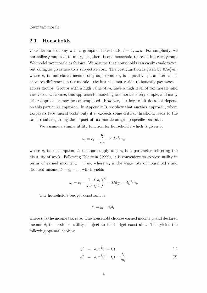
2.1 Households
Consider an economy with n groups of households, i = 1, ..., n. For simplicity, we
normalize group size to unity, i.e., there is one household representing each group.
We model tax morale as follows. We assume that households can easily evade taxes,
but doing so gives rise to a subjective cost. The cost function is given by 0.5e2imi,
where ei is undeclared income of group i and mi is a positive parameter which
captures differences in tax morale—the intrinsic motivation to honestly pay taxes—
across groups. Groups with a high value of mi have a high level of tax morale, and
vice versa. Of course, this approach to modeling tax morale is very simple, and many
other approaches may be contemplated. However, our key result does not depend
on this particular approach. In Appendix B, we show that another approach, where
taxpayers face ’moral costs’ only if ei exceeds some critical threshold, leads to the
same result regarding the impact of tax morale on group specific tax rates.
We assume a simple utility function for household i which is given by
ui = ci −l2i
2ai− 0.5e2
imi,
where ci is consumption, li is labor supply and ai is a parameter reflecting the
disutility of work. Following Feldstein (1999), it is convenient to express utility in
terms of earned income yi = liwi, where wi is the wage rate of household i and
declared income di = yi − ei, which yields
ui = ci −1
2ai
(yiwi
)2
− 0.5(yi − di)2mi.
The household’s budget constraint is
ci = yi − tidi,
where ti is the income tax rate. The household chooses earned income yi and declared
income di to maximize utility, subject to the budget constraint. This yields the
following optimal choices:
y∗i = aiw2i (1− ti), (1)
d∗i = aiw2i (1− ti)−
timi
. (2)
4
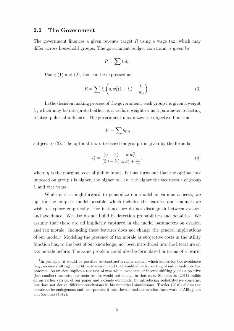
2.2 The Government
The government finances a given revenue target R using a wage tax, which may
differ across household groups. The government budget constraint is given by
R =∑
tidi.
Using (1) and (2), this can be expressed as
R =∑
ti
(aiw
2i (1− ti)−
timi
). (3)
In the decision making process of the government, each group i is given a weight
bi, which may be interpreted either as a welfare weight or as a parameter reflecting
relative political influence. The government maximizes the objective function
W =∑
biui
subject to (3). The optimal tax rate levied on group i is given by the formula
t∗i =(η − bi)(2η − bi)
aiw2i
aiw2i + 1
mi
, (4)
where η is the marginal cost of public funds. It thus turns out that the optimal tax
imposed on group i is higher, the higher mi, i.e. the higher the tax morale of group
i, and vice versa.
While it is straightforward to generalize our model in various aspects, we
opt for the simplest model possible, which includes the features and channels we
wish to explore empirically. For instance, we do not distinguish between evasion
and avoidance. We also do not build in detection probabilities and penalties. We
assume that these are all implicitly captured in the model parameters on evasion
and tax morale. Including these features does not change the general implications
of our model.7 Modeling the presence of tax morale as subjective costs in the utility
function has, to the best of our knowledge, not been introduced into the literature on
tax morale before. The same problem could also be formulated in terms of a ‘warm
7In principle, it would be possible to construct a richer model, which allows for tax avoidance(e.g., income shifting) in addition to evasion and that would allow for sorting of individuals into taxbrackets. As evasion implies a tax rate of zero while avoidance or income shifting yields a positive(but smaller) tax rate, our main results would not change in that case. Simonovits (2011) buildson an earlier version of our paper and extends our model by introducing redistributive concerns,but does not derive different conclusions in his numerical simulations. Traxler (2010) allows taxmorale to be endogenous and incorporates it into the seminal tax evasion framework of Allinghamand Sandmo (1972).
5

glow’ effect, i.e., the intrinsic satisfaction of doing the right thing when complying
with the tax law.
2.3 Hypothesis
Our theoretical model yields the following hypothesis:
Hypothesis: Group i’s efficient tax rate ti increases with group i’s tax morale
parameter mi.
Clearly, this hypothesis is well in line with standard results of optimal income tax
theory following Ramsey (1927) or Mirrlees (1971). Groups with a higher responsive-
ness to taxation should be taxed lower than groups with low levels of responsiveness,
i.e., a low elasticity of taxable income (e.g., Feldstein 1999 and Saez et al. 2011).
The next step in the analysis is to operationalize our hypothesis. This requires
us to classify individuals into groups as we argue that governments cannot observe
individual tax morale (which is private information). Policymakers only observe how
certain groups with certain observable characteristics respond to taxation. Further-
more, full discrimination in terms of taxation is neither legally nor economically
feasible. As we are interested in the personal income tax, a natural place to start is
income. For various reasons, governments levy different tax rates for different levels
of income (tax brackets) and hence tax distinct income groups differently. When
doing so they take into account that different income groups have different levels
of tax morale and adjust their taxation of the groups accordingly. Therefore, we
classify individuals by income groups and restate our hypothesis as follows:
Testable Hypothesis: Group i’s mean tax rate ti increases with group i’s mean
tax morale mi,
where ti and mi are ti and mi, respectively, mean-averaged across individuals within
income group i. This hypothesis can be tested with any data set that classifies
individuals by income and for which both tax rates and tax morale are available at
the income group or individual level.
3 Data and Operationalization
While we know of no single data set that jointly satisfies all the data requirements
mentioned in section 2.3, it is possible to construct such a data set using information
6

from different sources. In order to test our hypothesis empirically, we combine micro
data on tax morale and other covariates from the World Values Survey (WVS) and
European Values Survey (EVS) (EVS/WVS 2006; WVS 2009) with information on
tax rates from the World Tax Indicators (WTI) (Sabirianova-Peter et al. 2010).
Below we discuss each data source and define our measures of tax morale and tax
rates.
The WVS/EVS is the most common data source in tax morale research. It is
a worldwide survey which collects comparative data on many different values and
attitudes using standardized questionnaires for representative national samples of at
least 1000 respondents per country (Inglehart n.d.). The surveys are conducted by
professional scientific institutions and performed through face-to-face interviews at
the respondents’ home and in their respective national language.8 We employ all five
waves, which were carried out between 1981-1984, 1989-1993, 1994-1998, 1999-2004,
and 2005-2008, respectively.
Our key explanatory variable, tax morale, is measured by individuals’ re-
sponses to the following question:
Please tell me for the following statement whether you think it can always
be justified, never be justified, or something in between: ‘Cheating on
taxes if you have the chance’.
The question is measured on a ten-scale index with one (1) meaning ‘never
justifiable’ and ten (10) meaning ‘always justifiable’. Although this question has
been used very frequently in the literature to capture tax morale (e.g., Slemrod
2003, Alm and Torgler 2006, Richardson 2006 and Halla 2010), it is not free of bias.
For example, Andreoni et al. (1998) argue that people might overstate their degree
of morality in self-reports such as the WVS and those who have evaded might want
to excuse their behavior by declaring a high tax morale. Elffers et al. (1987) find
that there are significant differences between actual tax evasion and self-reported tax
evasion in surveys. Nevertheless, asking about tax morale is less blunt than asking
about tax evading behavior, and so the degree of honesty should be higher (Frey
and Torgler 2007). Another shortcoming of the question is the fact that taxpayers
might find tax evasion justifiable if tax revenue is used for, say, financing a dictator’s
war machine (Frey and Torgler 2007).
Nonetheless, previous robust evidence shows that low WVS levels of tax morale
are associated with high tax evasion and vice versa (Erard and Feinstein 1994;
Torgler and Schneider 2009; Halla 2010). This provides evidence in our favor of the
8Inglehart (2000) provides more comprehensive information on the WVS.
7
view that true tax evasion behaviour can be proxied with responses to questions
about tax morale. Hence, we think that it is appropriate to measure tax morale
with this question.
In addition, the WVS/EVS contains information on gross income for 10 income
groups (brackets).9 Therefore, we know each individual’s income group and tax
morale. We use this information to define two measures of tax morale for our
empirical analysis: i) ‘tax morale index’ represents income-group averages of the
original 10-scale variable as reported in the survey; ii) ‘tax morale dummy’ is based
on a dummy variable that is equal to 1 for individuals who report the highest level
of tax morale (1 on the original scale) and ‘0’ for individuals who report a value
greater than 1. It follows that ‘tax morale dummy’ is the share of individuals in
each income-group that report the highest possible level of tax morale.10 Both
variables are coded such that a higher value implies a higher level of tax morale.
Unlike tax morale, which is covered at the individual level across countries
and time in the WVS/EVS, tax rates at this level are more difficult to obtain. Of
course, statutory variables, such as the top marginal personal income tax rate, have
very wide country year coverage and are available from many sources. However,
our analysis requires tax rates that vary across time, countries, and income groups.
We rely on data from the recently published World Tax Indicator database to over-
come these challenges. This large and rather new panel data set covers personal
income tax structures at the country level in 189 countries for the period 1981 to
2005 (Sabirianova-Peter et al. 2010). Because it contains the complete national
income tax structures, including statutory rates, tax brackets, country-specific tax
formulae, standard deductions and tax credits among others, the data allow us to
compute average and marginal tax rates.11 More importantly, we are able to calcu-
late these tax rates for any level of gross income and hence at the income group levels
reported in the WVS/EVS.12 We use the raw WTI data to estimate average (AR)
and marginal (MR) tax rates for each income group reported in the WVS/EVS for
9The provided income steps are adjusted to the respective national income distributions, butthey do not reflect income deciles.
10This operationalization is commonly used (see, e.g., Alm and Torgler 2006 and Doerrenbergand Peichl 2011).
11The WTI collects tax schedule information for single tax payers only. This is not likely to haveany noticeable effect on the results since very few countries tax family income (exceptions includeGermany, France and the U.S.) or have tax schedules that depend on marital status (Sabirianova-Peter et al. 2010).
12A problem with the survey information is that we do not know whether individuals gave theincome reported to tax authorities or their true income. However, we are on the safe side since thepotential bias of tax evaders reporting their true income (low morale, high income, high tax rate)leads to an underestimation of the effect of tax morale on tax rates.
8

each country-year.13 Both tax rates adjust for standard deductions and credits and
are calculated using country specific tax formulae.14 Because there is no adjustment
for tax evasion or avoidance, these tax rates are close to, but are not, effective tax
rates. Nonetheless, they are superior to using statutory rates.
In order to relate the calculated income group tax rates to the WVS/EVS
data, all information from the WVS/EVS are aggregated (means) on the level of
country-year income groups. We restrict the sample to employed individuals before
aggregating the data, in an effort to limit our analysis to individuals who poten-
tially paid income taxes. We also exclude the respective lowest income group in
each country-year observation from our estimations as individuals in theses groups
usually do not pay income taxes; hence, we do not observe any variation in taxes
within and across these groups. Finally, the aggregated WVS/EVS information are
merged with the tax rates from the WTI. It seems reasonable to aggregate individual
information—including tax morale—on the income group level because i) it is very
unlikely that policy makers have individual level information on tax morale and ii)
even if they do, they could not tax each person individually. In addition, grouping
can alleviate measurement error in the covariates. Table 5 in the Appendix provides
summary statistics for the relevant variables.
4 Empirical Strategy and Results
This section describes our empirical strategy and results. In our regressions, we em-
ploy marginal (MR) and average (AR) tax rates as dependent variables and focus
on two main explanatory variables: ‘tax morale index’ and ‘tax morale dummy’.15
All estimations display panel-adjusted standard errors that account for clustering
effects of a certain country’s income groups and are robust to the presence of het-
eroscedasticity. The panel is highly unbalanced and many income groups are only
represented once, which makes it difficult to employ country fixed-effects.16
13Estimation is restricted to 52 countries that recorded gross income. For a sensitivity check(see section 5), we also estimate lead tax rates to analyze the impact of tax morale in year t ontax rates in t + 1.
14We are not able to adjust for deductions and credits that vary by individual characteristics(e.g., child credits). See Sabirianova-Peter et al. (2010) for a more detail description of the WTIand the tax rates.
15Recall that ‘tax morale dummy’ is the share of individuals in each income group that reportsthe highest level of tax morale whereas ‘tax morale index‘ is the average of the 10-point scale value.
16We show, however, that our hypothesis holds up to the inclusion of country-group fixed-effects,as well as actual country fixed-effects in estimations on the individual (person) level. See section5.1 for more details.
9

4.1 Empirical Model
OLS regressions, which are reported in Table 7 in the Appendix, provide evidence of
a positive association (conditional correlation) between group-level tax morale and
tax rates. This is consistent with our theoretical predictions. However, we believe
the OLS estimates are biased for reasons put forward below. Ex-ante, the direction
of the bias is not clear because the relationship between tax rates and tax morale is
found to be ambiguous in the literature (Torgler and Schneider 2007).
The first issue we have to address is reverse causality. While we aim to estimate
the effect of tax morale on tax rates, previous research has established a feedback
effect from tax rates (or the general system of taxation) to the level of tax morale
(see, e.g., Doerrenberg and Peichl 2011). Additionally, we are not able to control
for the actual extent of tax evasion or the size of the shadow economy. Since both
variables are known determinants of tax rates and tax morale, we must also contend
with omitted variable bias. Both issues imply OLS estimates are biased and that a
different identification strategy is required if we are to make any causal inference.
Therefore, we employ an instrumental variable, zijt, and estimate the model by two-
stage least squares (2SLS). An instrument that is sufficiently strongly correlated
with tax morale, but not with the error term in the structural equation of interest,
will provide us with exogenous variation, which can be exploited to overcome the
endogeneity problem and to identify the effect of interest. The first-stage regression
in our instrumental variable estimations reads
mijt = γ + ηzijt +Xδ + Cφ+ υi + θt + εijt, (5)
where subscripts i, j, and t indicate income group, country, and survey wave respec-
tively; zijt is one or both of our instruments (see section 4.2); mijt is one of our tax
morale measures (‘tax morale index’ or ‘tax morale dummy’); and υi, θt, and εijt are
income group dummies, survey wave dummies, and iid error terms, respectively.
Finally, X is a vector of income group control variables and C is a vector
of country-level control variables. X contains several confounding variables on the
income-group level: marital status, number of children, religiosity, and employment
status.17 All variables in X are obtained from the WVS/EVS and averaged over
17 These are known determinants of tax morale and tax rates (e.g. Torgler 2007). Note thatthe theoretical relationship between income and tax morale is not clear (see Doerrenberg andPeichl 2011). On the one hand, evasion yields higher returns for high-income earners—especiallyin countries with progressive tax systems. On the other, people earning high incomes might havehigher societal stakes and therefore be more affected by sanctions, i.e., losing a well-paid job.Accordingly, the empirical picture is ambiguous as well. Whereas Konrad and Qari (2009) cannotfind any significant effects using European data, a negative relationship is found by Torgler (2006)for a larger set of countries.
10

income groups. We include GDP per capita (in PPP), GDP growth rate, and foreign
direct investments (FDI) in vector C in order to account for confounding country-
level variables. All country-level variables are taken from the Worldbank’s World
Development Indicators (World Bank 2010). Our specification hence exploits across-
country and within-country variation in tax morale to explain heterogenous levels
of tax rates.
Intuitively, the IV estimations will use the fitted values from the first-stage
equation (5) as substitutes for mijt in the following OLS regression of tax rates on
income group’s characteristics:
tijt = α + βmijt +Xδ + Cφ+ υi + θt + εijt, (6)
where mijt is one of our tax morale measures but instrumented by zijt, and tijt is
one of our tax rate measures (AR or MR). Hence, the identification of the impact
of tax morale on tax rates will rely only on that part of the variation in mijt, which
is driven by exogenous variables.
4.2 Instruments
Finding suitable instruments is generally a difficult task. We require an instrument
that is related to income group tax morale, but does not have any link to the same
income group’s tax rate. Given the structure of our dataset, we also require the
instrument to have sufficient variation across income groups. We mainly employ
two instruments in our IV estimations, which we base on other questions asked in
the WVS/EVS:18
Dodging fares justifiable? For our first instrument we exploit the answer to the
question: ‘Tell me whether you think it can always be justified, never be justified
or something in between, to avoid a fare on public transportation’. Respondents
are asked to respond to the question on a 10 point scale. The instrument and tax
morale are fairly correlated and we do not suffer from a weak instrument (see below).
Of course, many individuals who report high tax morale also develop a high level
of ‘dodging-fares-morale’ and hence we are able to observe a positive relationship
between the two variables.
As for exclusion restriction, we assume that the share of people in each income
group who have a high ‘dodging-fares-morale’ is not related to their tax rate. A pos-
18Lubian and Zarri (2011) also use tax morale as an explanatory variable (to explain happiness)and instrument it with another question from the same survey. They, however, use a differentdataset (for Italy) and their instrument is not available in our data.
11
sible drawback occurs for countries where public transportation is operated by the
government and where taxes and public transportation are financed from the same
budget: if, in those countries, many people dodge fares, the transportation sector
might have to be cross-subsidized by tax money; implying that, ceteris paribus, taxes
might be higher in such countries. However, in most countries public transporta-
tion is privately or semi-privately run. In the latter case, usually the transportation
companies are on a different budget than the tax legislating government.
Child unselfishness Our second instrument is based on a question concerning
attitudes on educating and raising one’s own children: ‘Here is a list of qualities
that children can be encouraged to learn at home. Which, if any, do you consider
to be especially important? ’ As an instrument, we use the share of people in each
income group who replied that ‘unselfishness’ is one of the key qualities children
should be encouraged to learn. As we would expect intuitively, this variable is also
fairly positively correlated with tax morale. Paying taxes can be seen as a service
to society: taxes finance public goods and social benefits. Individuals who have low
tax morale and tend to evade their taxes are less likely to believe that it is especially
important for their children to develop an unselfishness character.
We also assume the exclusion restriction holds: The share of people who believe
that unselfishness is important should not affect the level of taxes. What is more,
we do not expect reverse causality problems either. The answer to this question
is not affected by the tax system or tax rates. The question for unselfishness of
children is located in a different module (A) of the survey than the questions for the
justifiability of tax evasion and dodging fares (module F). This leads us to believe
the replies to both questions were given independently of each other.
Validity of instruments and 1st-stage results Instruments need to satisfy two
conditions: they must be correlated with the endogenous variable and orthogonal
to the error term. We have to rely on economic theory and intuitive reasoning to
back the latter (see the discussion above). The former can, however, be tested by
looking at the first-stage results of regressions of the instrumented variable—tax
morale—on all exogenous variables and the instruments. Tables 8 and 9 in the ap-
pendix display first-stage results of our baseline specifications. As expected, both
instruments—‘dodging fares justifiable?’ and ‘child unselfishness’—have a signifi-
cant positive impact on tax morale after conditioning on all confounding variables.
The first-stage results hence confirm our intuition given above.
The F-statistics of excluded instruments—reported in Tables 1 and 2—are well
12

larger than 10 when ‘cheating on public transportation’ is used as the instrument.19
The respective F-statistics for specifications with ‘child unselfishness’ alone are lower:
estimations employing ‘tax morale index’ as the instrumented variable display F-
statistics of around 7, whereas they are slightly larger than 10 (around 13) when ‘tax
morale dummy’ is the endogenous variable.20 Our over-identified estimations, where
we use both available instruments, disclose F-statistics of excluded instruments of
above 40; thus putting us in the ‘safe zone’. Finally, for our overidentified estimations
we mostly cannot reject the null hypotheses of the Hansen test of overidentification
at reasonable levels of significance. An exception is the estimation with AR serving
as the dependent variable and tax morale index being the explanatory variable where
we can only reject the null hypothesis at the 6% level (the corresponding p-values
are reported in the result tables below).
4.3 Baseline Results
Baseline results using 2SLS are presented in Tables 1 and 2 for AR and MR, re-
spectively. The results confirm our hypothesis. For both operationalizations of
our main explanatory variable—tax morale on the 10-point scale and ‘tax morale
dummy’ based on a dummy with 1 standing for the highest level of tax morale—we
observe that a higher level of tax morale is associated with, ceteris paribus, higher
taxation. Increasing ‘tax morale index’ by one standard deviation in the ‘cheat-
ing’ specification increases the tax rate by 0.6 standard deviations. The estimate
is significantly different from zero at the 1% level. The point estimates are higher,
but less significant when ‘child unselfishness’ is employed to instrument tax morale:
a one standard deviation increase in ‘tax morale index’ increases the tax rate by
1.09 standard deviations. In the overidentified case, where we use both available
instruments, the coefficient is highly significant and very close to the point estimate
in the ‘cheat’ specification.
19IV estimations are prone to be biased and inconsistent if the correlation between instrumentand instrumented variable is too weak and if there are many over-identifying restrictions (Boundet al. 1995). Staiger and Stock (1997) suggest that F-statistics of excluded instruments need tobe larger than 10 to exclude a problem of weak instruments.
20The former figure might indicate a weak instrument problem. However, Angrist and Pischke(2009a, page 215) note that this is not a mechanical rule and F-statistics smaller than 10 might notalways be fatal. In the just-identified case—say, one endogenous variable and one instrument—thetwo-stage-least-squares (2SLS) estimates are approximately unbiased (median-unbiased) and weakinstrument problems only cause second-stage standard errors to be large (Angrist and Pischke2009a; Angrist and Pischke 2009b, page 209). Even in those specifications with the smallest F-statistics, we obtain decently small standard errors suggesting that we do not suffer from a weakinstrument problem.
13

Table 1: Effect of Tax Morale on Average Tax Rates
Cheat Unself Both Cheat Unself Both
Tax morale index 10.557*** 19.185** 11.486***
(2.397) (9.239) (2.399)
Tax morale dummy 52.257*** 61.357*** 56.071***
(11.640) (22.768) (10.909)
Income group 3 0.272 −0.118 −0.067 1.381 1.387 1.074
(3.616) (4.200) (3.730) (3.525) (3.449) (3.627)
Income group 4 0.434 −0.279 −0.093 1.826 2.069 1.359
(3.707) (4.510) (3.855) (3.577) (3.473) (3.702)
Income group 5 2.198 1.289 1.581 2.723 2.358 2.078
(3.872) (4.461) (4.024) (3.833) (3.731) (3.976)
Income group 6 4.773 4.276 4.200 5.454 5.086 4.846
(3.914) (4.517) (4.076) (3.836) (3.766) (3.984)
Income group 7 7.504* 7.571* 6.754* 8.702** 8.530** 8.002**
(3.871) (4.540) (4.072) (3.787) (3.764) (3.970)
Income group 8 10.208*** 10.385** 9.596** 11.171*** 10.648*** 10.505***
(3.662) (4.397) (3.851) (3.574) (3.657) (3.747)
Income group 9 12.548*** 12.804*** 12.021*** 13.094*** 12.530*** 12.769***
(3.877) (4.799) (4.077) (3.790) (3.896) (3.971)
Income group 10 16.236*** 18.217*** 16.132*** 16.140*** 15.767*** 15.890***
(3.800) (5.804) (3.964) (3.591) (4.022) (3.741)
GDP per capita 0.419*** 0.361*** 0.414*** 0.531*** 0.469*** 0.537***
(0.125) (0.124) (0.131) (0.128) (0.111) (0.132)
GDP growth −0.134 −0.390 −0.163 −0.052 −0.178 −0.086
(0.231) (0.286) (0.239) (0.230) (0.218) (0.240)
FDI, net inflows −0.033*** −0.012 −0.032*** −0.042*** −0.034*** −0.041***
(0.009) (0.019) (0.009) (0.008) (0.008) (0.008)
constant −57.419*** −119.234* −64.283*** −6.245 −8.819 −7.752
(20.087) (66.986) (20.093) (11.084) (13.900) (11.029)
N 504 567 495 504 567 495
F-stat excl. instr 91.47 6.96 49.88 74.53 13.65 43.26
p-val Hansen overid / / 0.06 / / 0.14
[1] Dep. Variable: AR [2] 2SLS estimations [3] Instruments: ‘Dodging fares justifiable‘, ‘Child unselfishness‘
or both [4] Cluster-adjusted standard errors [5] Sociodemographic controls and wave dummies included but not
displayed [6] Income group 2 is reference category [7] ∗ < 0.10, ∗∗ < 0.05, ∗ ∗ ∗ < 0.01 [8] First-stage
results shown in Table 8 in the appendix
Of course, the absolute coefficients on ‘tax morale dummy’ are much larger
than on ‘tax morale index’. With this dummy being the independent and instru-
mented variable, the coefficient stands for a change from the lowest to the highest
level of tax morale. A one standard deviation increase in ‘tax morale dummy’ in-
14

creases the tax rate by 0.61 in the ‘cheat’ specification and 0.72 standard deviations
in the ‘unselfishness’ specification. The point estimate in the overidentified model
lies between the coefficients in the just-identified models and is significantly different
from zero at the 1% level. Again, the coefficient stemming from the overidentidfied
estimation is very close to the corresponding one in the ‘cheat’ specification. It is
clear, then, that the results are in accordance with the ‘tax morale index’ specifica-
tions.
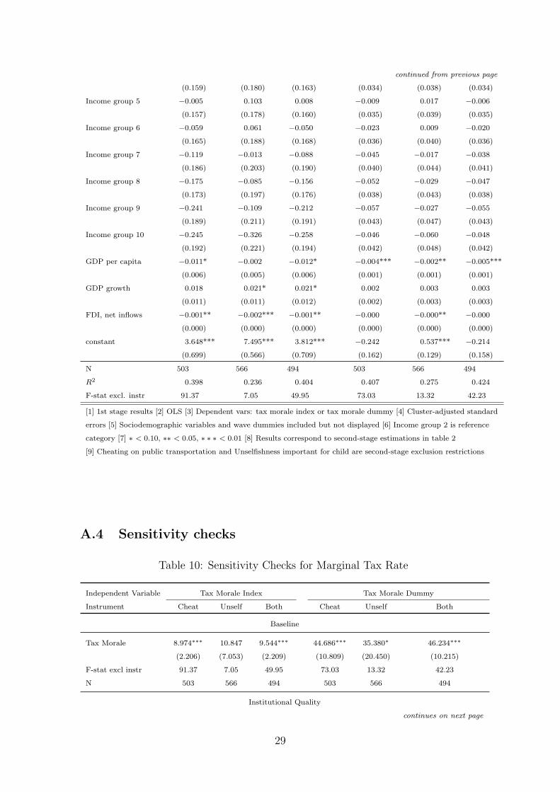
Table 2 presents the results with the marginal tax rate (MR) as the dependent
variable. The results and patterns are very similar to those described above. An
increase in ‘tax morale index’ (‘tax morale dummy’) by one standard deviation
increases MR by 0.51 (0.53) standard deviations with ‘cheat’ as the IV and by 0.62
(0.42) in the ‘unselfishness’ specification. The low conditional correlation between
‘unselfishness’ and ‘tax morale’ causes the coefficient in specification 2 not to be
significant on the 10% level; the corresponding p-value is 0.12 and therefore very close
to being significant. The overidentified estimation yields highly significant estimates
that are very close to the corresponding values in the just-identified cases. In the
latter three specifications, where ‘tax morale dummy’ serves as the explanatory
variable, all three coefficients of interest are positive and significant. While the
coefficient in the ‘unself’ specification was slightly insignificant with ‘tax morale
index’ as the explanatory variable, the respective coefficient is now significant at the
10% level.
Table 2: Effect of Tax Morale on Marginal Tax Rates
cheat unself both cheat unself both
Tax morale index 8.974*** 10.847 9.544***
(2.206) (7.053) (2.209)
Tax morale dummy 44.686*** 35.380* 46.234***
(10.809) (20.450) (10.215)
Income group 3 4.884 5.323 4.651 5.722 6.069* 5.492
(3.566) (3.524) (3.659) (3.480) (3.206) (3.555)
Income group 4 5.711 6.167* 5.286 6.786* 7.384** 6.384*
(3.698) (3.715) (3.820) (3.595) (3.269) (3.691)
Income group 5 9.072** 8.977** 8.492** 9.420** 9.477*** 8.809**
(3.793) (3.755) (3.921) (3.745) (3.445) (3.854)
Income group 6 13.221*** 13.189*** 12.683*** 13.705*** 13.550*** 13.120***
(3.655) (3.536) (3.791) (3.582) (3.224) (3.695)
Income group 7 16.040*** 16.144*** 15.375*** 16.975*** 16.615*** 16.308***
(3.610) (3.525) (3.776) (3.522) (3.229) (3.662)
Income group 8 18.719*** 18.492*** 18.177*** 19.465*** 18.580*** 18.835***
(3.507) (3.496) (3.659) (3.428) (3.241) (3.560)
Income group 9 20.703*** 20.343*** 20.184*** 21.099*** 20.130*** 20.708***
continues on next page
15
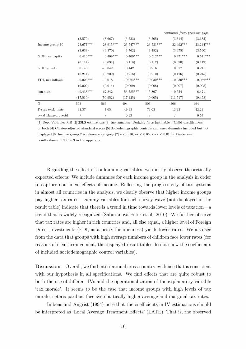
continued from previous page
(3.579) (3.667) (3.733) (3.505) (3.314) (3.632)
Income group 10 23.677*** 23.915*** 23.547*** 23.531*** 22.492*** 23.244***
(3.633) (4.370) (3.762) (3.482) (3.475) (3.590)
GDP per capita 0.416*** 0.409*** 0.409*** 0.512*** 0.471*** 0.511***
(0.114) (0.091) (0.118) (0.117) (0.090) (0.119)
GDP growth 0.146 −0.042 0.142 0.216 0.077 0.211
(0.214) (0.209) (0.218) (0.210) (0.176) (0.215)
FDI, net inflows −0.025*** −0.018 −0.024*** −0.032*** −0.030*** −0.032***
(0.009) (0.014) (0.009) (0.008) (0.007) (0.008)
constant −49.433*** −62.842 −53.785*** −5.867 −0.554 −6.421
(17.510) (50.952) (17.425) (9.605) (11.517) (9.458)
N 503 566 494 503 566 494
F-stat excl. instr 91.37 7.05 49.95 73.03 13.32 42.23
p-val Hansen overid / / 0.32 / / 0.57
[1] Dep. Variable: MR [2] 2SLS estimations [3] Instruments: ‘Dodging fares justifiable‘, ‘Child unselfishness‘
or both [4] Cluster-adjusted standard errors [5] Sociodemographic controls and wave dummies included but not
displayed [6] Income group 2 is reference category [7] ∗ < 0.10, ∗∗ < 0.05, ∗ ∗ ∗ < 0.01 [8] First-stage
results shown in Table 9 in the appendix
Regarding the effect of confounding variables, we mostly observe theoretically
expected effects: We include dummies for each income group in the analysis in order
to capture non-linear effects of income. Reflecting the progressivity of tax systems
in almost all countries in the analysis, we clearly observe that higher income groups
pay higher tax rates. Dummy variables for each survey wave (not displayed in the
result table) indicate that there is a trend in time towards lower levels of taxation—a
trend that is widely recognized (Sabirianova-Peter et al. 2010). We further observe
that tax rates are higher in rich countries and, all else equal, a higher level of Foreign
Direct Investments (FDI, as a proxy for openness) yields lower rates. We also see
from the data that groups with high average numbers of children face lower rates (for
reasons of clear arrangement, the displayed result tables do not show the coefficients
of included sociodemographic control variables).
Discussion Overall, we find international cross-country evidence that is consistent
with our hypothesis in all specifications. We find effects that are quite robust to
both the use of different IVs and the operationalization of the explanatory variable
‘tax morale’. It seems to be the case that income groups with high levels of tax
morale, ceteris paribus, face systematically higher average and marginal tax rates.
Imbens and Angrist (1994) note that the coefficients in IV estimations should
be interpreted as ‘Local Average Treatment Effects’ (LATE). That is, the observed
16

effect is the effect of the so-called complier population (see also Angrist et al. 1996).
In our case, this implies that the reported coefficients are restricted to the sub-
sample of individuals that would change their level of tax morale in response to a
hypothetical change in the instruments. The IV approach prevents the hazard of
reverse causality as we assume the instruments to be unrelated to the dependent
variables. However, depending on which instrument is used, we observe different
magnitudes in coefficients. This should be a sign of caution indicating that we cannot
take the actual magnitude of the coefficients for granted. The robust positive sign,
nevertheless, provides evidence backing our hypothesis. Even in those specifications
with low F-statistics of excluded instruments, and hence higher standard errors, we
do not expect the results to be biased as they are just-identified.
5 Sensitivity Checks
We conduct two broad categories of robustness checks in order to increase confidence
in our results. First, we examine the source of variation used to identify the effect
of tax morale by estimating models with regional fixed effects and country fixed
effects. These extensions are particularly important since the theoretical model
focuses on within country variation. The second category addresses other important,
but relatively minor issues that might affect our results. We describe each of these
categories—in turn, starting with fixed effect models.
5.1 Fixed Effects Models
It is possible that our results are driven by genuine differences between countries,
rather than within country variation, which we are also exploiting. For example,
results may be biased if high-tax countries also happen to have high average levels
of tax morale and the instrumental variables. To check this, we employ fixed-effects
regressions.21 Running country-fixed-effect estimations in our case, however, causes
problems of multicollinearity and too few degrees of freedom because the sample is
highly unbalanced; many countries participated in only one wave of the WVS/EVS.
We address this problem in two ways. First, following the WVS/EVS literature (e.g.
Helliwell 2003), we form groups of countries to reduce the number of country fixed-
effect variables. We then estimate a country-group fixed-effects model with eight
country groups: English-speaking countries (Anglo-Saxon plus Australia and New
Zealand); Continental Europe plus Israel; Scandinavia; Eastern Central Europe;
21Note, however, that we indirectly account for some country-specific effects in our previousestimations by including country-level control variables in all of our regressions.
17
former Soviet countries; Latin America; Asia; and (other) Developing Countries
(see Table 6 for an overview of country-groups). As shown in Panel A of Table
3, the country-group fixed-effect estimations yield coefficients that are very close
(and also significant) to the baseline specification when ‘cheat’ is employed as the
instrument.22
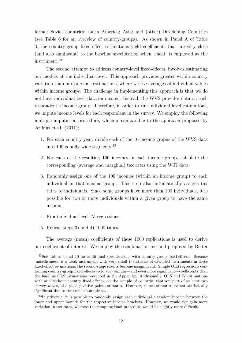
The second attempt to address country-level fixed-effects, involves estimating
our models at the individual level. This approach provides greater within country
variation than our previous estimations, where we use averages of individual values
within income groups. The challenge in implementing this approach is that we do
not have individual level data on income. Instead, the WVS provides data on each
respondent’s income group. Therefore, in order to run individual level estimations,
we impute income levels for each respondent in the survey. We employ the following
multiple imputation procedure, which is comparable to the approach proposed by
Jenkins et al. (2011):
1. For each country year, divide each of the 10 income gropus of the WVS data
into 100 equally wide segments.23
2. For each of the resulting 100 incomes in each income group, calculate the
corresponding (average and marginal) tax rates using the WTI data.
3. Randomly assign one of the 100 incomes (within an income group) to each
individual in that income group. This step also automatically assigns tax
rates to individuals. Since some groups have more than 100 individuals, it is
possible for two or more individuals within a given group to have the same
income.
4. Run individual level IV-regressions.
5. Repeat steps 3) and 4) 1000 times.
The average (mean) coefficients of these 1000 replications is used to derive
our coefficient of interest. We employ the combination method proposed by Reiter
22See Tables 4 and 10 for additional specifications with country-group fixed-effects. Because‘unselfishness’ is a weak instrument with very small F-statistics of excluded instruments in thesefixed-effect estimations, the second-stage results become insignificant. Simple OLS regressions con-taining country-group fixed effects yield very similar—and even more significant—coefficients thanthe baseline OLS estimations presented in the Appendix. Additionally, OLS and IV estimationswith and without country fixed-effects, on the sample of countries that are part of at least twosurvey waves, also yield positive point estimates. However, these estimates are not statisticallysignificant due to the smaller sample size.
23In principle, it is possible to randomly assign each individual a random income between thelower and upper bounds for the respective income brackets. However, we would not gain morevariation in tax rates, whereas the computational procedure would be slightly more difficult.
18

(2003), and applied by Jenkins et al. (2011), to calculate standard-errors and levels
of significance, taking into account the finite number of imputations.
Step 4 includes the following control variables; i) the same individual-level
controls as in the baseline, ii) survey wave fixed-effects, iii) income group fixed-
effects, and iv) country fixed-effects. We exclude country-level variables from our
estimations in order to use the full sample of countries, including those that are only
part of one WVS wave. Due to the insignificant results of the ’child’ instrument in
the country-group fixed-effects estimation (see Section 5.2), and for brevity, we focus
on the ’cheat’ instrument here. Results from this multiple-imputation regression
approach are presented in Panels B and C of Table 3.24
Table 3: Fixed-Effect Estimations
Expl. Variable Tax Morale Index Tax Morale Dummy
Dependent Variable AR MR AR MR
Panel A: Income-group level with Country-Group Fixed-Effects
Tax Morale 10.506∗∗∗ 8.889∗∗∗ 67.365∗∗∗ 57.547∗∗∗
(2.494) (2.348) (17.077) (16.080)
Observations 504 503 504 503
Panel B: Multiple Imputation Approach without Country Fixed-Effects
Tax Morale 1.0584∗∗∗ 0.8130∗∗∗ 5.8698∗∗∗ 4.5089∗∗∗
(0.2579) (0.2615) (1.4077) (1.4333)
Panel C: Multiple Imputation Approach with Country Fixed-Effects
Tax Morale 0.1736∗∗∗ 0.1562∗∗∗ 0.9681∗∗∗ 0.8710∗∗∗
(0.0516) (0.0503) (0.2847) (0.2788)
Observations 33,022 33,022 33,022 33,022
[1] 2SLS IV regressions [2] Instrument: Cheating on Public Transportation
[3] Panel A: Income-group level estimations include same control variables
as the baseline specifications [4] Panels B and C: Individual level
estimations based on multiple imputation approach. ’Observations’ is number
of observations per random draw. Control variables as in baseline, but w/o
country-level variables. Standard errors in parentheses are calculated
following Reiter (2003) [5] ∗ < 0.10, ∗∗ < 0.05, ∗ ∗ ∗ < 0.01
The multiple imputation approach yields coefficients that are an order of mag-
24The results from this multiple-imputation regression approach are similar to those obtainedfrom an interval regression, in which we use the lower and upper bounds of the tax rate bracketson the individual level as dependent variables.
19
nitude smaller than the income group estimates reported in Tables 1 and 2. This
can be explained by the increased variation in the explanatory variables (as well
as the dependent variable).25 Nonetheless, the coefficients—for both ’tax morale
index’ and ’tax morale dummy’—are positive and statistically different from zero.
More importantly, this result holds when we include country fixed-effects. Since
all country specific effects are captured and controlled for in Panel C, the positive
coefficients can be attributed solely to within-country variation in tax morale. This
provides further evidence that our results are not being driven by between country
variation. The importance of between country variation can be seen by comparing
the coefficients in Panels B and C.
5.2 Other Robustness Checks
In our second set of robustness checks, we go back to income-group level estimations
and first include a country level measure of bureaucratic quality (ICRG 2011)—a
variable found to be a possible determinant of tax morale (Barone and Mocetti
2011)—in order to control for the possibility that countries with less efficient gov-
ernments have higher tax rates (Brennan and Buchanan 1980).26 We also run re-
gressions in which we weight the income groups by the number of their members.
Additionally, we restrict the analysis to OECD countries in order to gain insights for
a more homogeneous set of countries. Finally, we employ lead tax rates where tax
rates in year t+ 1 are related to tax morale in year t. Tables 4 (dependent variable:
AR) and 10 (dependent variable: MR; table displayed in the Appendix) summarize
these sensitivity checks.
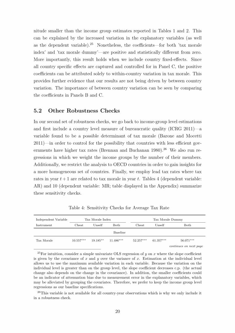
Table 4: Sensitivity Checks for Average Tax Rate
Independent Variable Tax Morale Index Tax Morale Dummy
Instrument Cheat Unself Both Cheat Unself Both
Baseline
Tax Morale 10.557∗∗∗ 19.185∗∗ 11.486∗∗∗ 52.257∗∗∗ 61.357∗∗∗ 56.071∗∗∗
continues on next page
25For intuition, consider a simple univariate OLS regression of y on x where the slope coefficientis given by the covariance of x and y over the variance of x. Estimation at the individual levelallows us to use the maximum available variation in each variable. Because the variation on theindividual level is greater than on the group level, the slope coefficient decreases c.p. (the actualchange also depends on the change in the covariance). In addition, the smaller coefficients couldbe an indicator of attenuation bias due to measurement error in the explanatory variables, whichmay be alleviated by grouping the covariates. Therefore, we prefer to keep the income group levelregressions as our baseline specifications.
26This variable is not available for all country-year observations which is why we only include itin a robustness check.
20

continued from previous page
(2.397) (9.239) (2.399) (11.640) (22.768) (10.909)
F-stat excl instr 91.47 6.96 49.88 74.53 13.65 43.26
N 504 567 495 504 567 495
Institutional Quality
Tax Morale 12.155∗∗∗ 20.313∗∗ 13.256∗∗∗ 61.694∗∗∗ 77.945∗∗∗ 65.858∗∗∗
(2.489) (9.702) (2.466) (12.153) (30.114) (11.494)
Institutional Quality -5.824∗∗∗ -5.435∗∗∗ -6.018∗∗∗ -8.534∗∗∗ -8.265∗∗∗ -8.962∗∗∗
(1.681) (2.052) (1.767) (1.587) (1.968) (1.643)
F-stat excl instr 84.96 6.70 45.86 75.40 9.49 41.66
N 464 527 455 464 527 455
Weighted
Tax Morale 10.641∗∗∗ 46.330∗ 12.003∗∗∗ 52.761∗∗∗ 118.831∗∗∗ 62.234∗∗∗
(2.648) (25.493) (2.750) (12.500) (42.548) (12.664)
F-stat excl instr 75.54 3.41 39.48 78.58 10.22 43.38
N 502 565 493 502 565 493
OECD Countries
Tax Morale 15.290∗∗∗ 24.816∗∗∗ 15.904∗∗∗ 77.437∗∗∗ 80.356∗∗∗ 80.066∗∗∗
(2.778) (8.520) (2.700) (13.814) (21.219) (12.422)
F-stat excl instr 64.14 9.98 37.81 52.06 17.07 33.27
N 385 421 385 385 421 385
Lead Tax Rates
Tax Morale 8.981∗∗∗ 18.529∗∗ 9.656∗∗∗ 43.951∗∗∗ 60.183∗∗∗ 47.555∗∗∗
(2.357) (9.342) (2.316) (11.104) (23.343) (10.576)
F-stat excl instr 80.90 6.82 46.22 69.01 13.43 40.30
N 477 549 477 477 549 477
Country-Groups Fixed Effects
Tax Morale 10.506∗∗∗ -74.937 8.390∗∗∗ 67.365∗∗∗ -991.359 52.371∗∗∗
(2.494) (65.262) (2.418) (17.077) (2281.237) (15.642)
F-stat excl instr 77.96 1.26 36.84 44.86 0.18 22.29
N 504 567 495 504 567 495
[1] Dep. Var. AR [2] 2SLS IV estimations [3] Cluster-adjusted standard errors [4] All estimations include
same control variables as in baseline specifications. [5] Country-Group Fixed Effects contain dummies for regional
country groups. [6] Lead tax rates estimations are IV regressions of tax rates in year t+ 1 on tax morale in
t. [7] Weighted IV regressions weight income groups with the number of individuals in each respective group
[8] ∗ < 0.10, ∗∗ < 0.05, ∗ ∗ ∗ < 0.01
We are able to confirm our baseline results in almost all sensitivity checks.
Tax rates, ceteris paribus, depend positively on the level of tax morale and the
results are mostly significantly different from zero. In most specifications, the size
21

of the tax morale point estimates is roughly similar to the sizes in the baseline.
Interestingly, when the sample is restricted to OECD countries, we find significant
point estimates that are slightly larger than in the baseline scenario. Additionally,
we confirm Brennan and Buchanan’s (1980) argument of a negative relationship
between tax rates and the quality of bureaucracy.
6 Conclusion
In this paper, we construct an international panel dataset of (average and marginal)
tax rates and tax morale parameters in order to provide evidence of the relationship
between tax morale and the tax burden imposed on different income groups. We set
up a simple model of Ramsey-type optimal income taxation where different groups
of taxpayers face different subjective costs of evading taxes. The model shows that
the tax rate imposed on a group will be higher, the higher the group’s tax morale,
i.e., the less responsive tax base will be taxed at higher rates. Using data from the
EVS/WVS and the WTI and based on an IV approach, we find empirical support for
this hypothesis. Our results show that ‘nice guys finish last’, i.e., groups with higher
tax morale have to bear a higher tax burden. Several robustness checks validate our
baseline results.
From the government’s perspective, this distribution of taxes is efficient be-
cause the costs of taxation—caused by distortions—are smaller for individuals with a
high tax morale. Our paper therefore relates to the growing literature on elasticities
of taxable income (Feldstein 1999; Saez et al. 2011). If the tax morale parameter is
interpreted as a proxy for the tax evasion elasticity, our empirical results show that
the actual distribution of tax burdens is indeed associated with these elasticities,
i.e., that governments take this information into account when designing actual tax
systems. This provides an empirical test of the inverse elasticity rule of optimal
taxation, which is another contribution of our paper.
Our findings also shed new light on the growing literature on tax morale. So far,
scholars have mostly argued that a high general level of tax morale is advantageous
for a society because it increases the efficiency of a tax system. Many empirical
studies have worked out possible determinants of tax morale and derived the policy
implication that strengthening these determinants helps to increase tax morale and
therefore the efficiency of raising taxes. While we do not contradict this view, we
show that governments already seem to exploit high relative levels of tax morale
among particular groups and, ceteris paribus, tax them higher than low morale
groups in the same country. The welfare implications of this finding are, however,
22

less clear. Despite being taxed more heavily, such a policy might still be welfare
improving even for high morale groups if they receive some kind of ‘warm glow’ effect
due to the intrinsic satisfaction of doing the right thing when complying with the tax
law. It would also be interesting to extend the analysis to allow for endogenous levels
of tax morale (see, e.g., Traxler 2010, who incorporates tax morale endogenously into
the standard model of tax evasion). A tax policy as sketched in our study is likely
to be self defeating in the long term in that it creates incentives to develop a lower
level of tax morale. Exploring this is a topic for future research.
23

A Appendix
A.1 Summary Statistics
Table 5: Summary statistics
Variable Mean Std. Dev. N
Average Tax Rate (AR) 24.191 15.243 694
Marginal Tax Rate (MR) 30.483 15.179 693
AR lead 24.483 15.584 650
MR lead 30.619 15.3 649
Tax morale index 8.420 0.863 685
Tax morale dummy 0.562 0.179 685
Cheat public transp 8.424 0.846 606
Unself imp for child 0.31 0.171 692
Full time 0.718 0.172 701
Part time 0.125 0.097 701
Self employed 0.157 0.159 701
Single 0.287 0.141 701
Married 0.637 0.171 701
Divorced 0.052 0.074 701
Widowed 0.023 0.041 701
Age 38.99 3.776 701
Number children 1.758 0.559 692
Age at compl educ 19.408 3.299 598
Church once month 0.336 0.24 686
GDP per cap, ppp 18.453 11.142 701
GDP growth 2.82 3.463 701
FDI, net inflows 11.018 63.623 701
Institutional quality 3.089 0.933 624
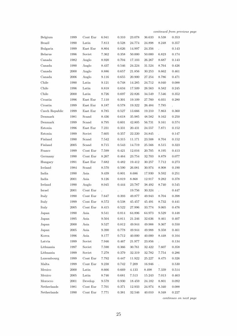
Table 6: Means of key variables by country and year
Country Year Group TM-10 TM AR MR cheat unself
Albania 2002 East Eur 9.079 0.587 17.672 21.972 8.583 0.134
Australia 1995 Anglo 8.616 0.563 44.611 46.441 8.819 0.400
Australia 2005 Anglo 8.701 0.546 23.058 33.248 8.361 0.502
Austria 1999 Cont Eur 8.687 0.553 21.224 33.229 8.509 0.042
Belgium 1990 Cont Eur 6.290 0.261 24.841 39.387 8.217 0.272
continues on next page
24
continued from previous page
Belgium 1999 Cont Eur 6.941 0.310 23.078 36.633 8.538 0.353
Brazil 1990 Latin 7.813 0.528 24.774 24.898 8.248 0.357
Bulgaria 1999 East Eur 8.804 0.626 14.997 24.356 . 0.143
Belarus 1996 Soviet 7.362 0.358 50.000 50.000 6.823 0.174
Canada 1982 Anglo 8.920 0.704 17.103 26.267 8.687 0.143
Canada 1990 Anglo 8.437 0.546 24.224 31.524 8.764 0.426
Canada 2000 Anglo 8.886 0.657 21.856 30.253 8.662 0.461
Canada 2006 Anglo 9.116 0.655 20.900 27.254 8.786 0.471
Chile 1990 Latin 9.121 0.748 14.285 24.712 8.040 0.088
Chile 1996 Latin 8.818 0.634 17.509 28.563 8.582 0.245
Chile 2000 Latin 8.726 0.697 22.826 34.549 7.546 0.352
Croatia 1996 East Eur 7.110 0.301 19.109 27.760 6.031 0.280
Croatia 1999 East Eur 8.187 0.578 19.322 26.484 7.785 .
Czech Republic 1999 East Eur 8.785 0.527 13.666 19.210 7.863 0.360
Denmark 1981 Scand 8.436 0.618 35.985 48.582 9.162 0.250
Denmark 1999 Scand 8.795 0.601 42.805 56.731 9.161 0.574
Estonia 1996 East Eur 7.231 0.331 20.431 24.557 7.871 0.152
Estonia 1999 Soviet 7.605 0.357 22.220 24.845 . 0.147
Finland 1990 Scand 7.542 0.315 11.171 23.508 8.704 0.152
Finland 2005 Scand 8.715 0.543 14.719 25.566 8.515 0.323
France 1999 Cont Eur 7.599 0.421 12.016 20.705 8.195 0.413
Germany 1990 Cont Eur 8.267 0.464 23.754 32.703 8.879 0.077
Hungary 1991 East Eur 7.682 0.482 19.412 30.257 7.712 0.273
Iceland 1984 Scand 8.570 0.590 26.081 30.974 8.908 0.190
India 1990 Asia 9.439 0.801 8.686 17.930 9.592 0.251
India 2001 Asia 9.126 0.819 8.868 12.917 9.282 0.378
Ireland 1990 Anglo 8.045 0.444 23.787 38.492 8.740 0.545
Israel 2001 Cont Eur . . 19.756 30.324 . 0.447
Italy 1990 Cont Eur 7.647 0.393 49.877 49.943 8.704 0.398
Italy 1999 Cont Eur 8.572 0.538 45.457 45.491 8.732 0.441
Italy 2005 Cont Eur 8.415 0.522 27.996 33.774 9.065 0.476
Japan 1990 Asia 9.541 0.814 64.896 64.973 9.529 0.448
Japan 1995 Asia 9.504 0.811 21.246 32.636 9.461 0.407
Japan 2000 Asia 9.527 0.812 49.944 49.988 9.367 0.550
Japan 2005 Asia 9.390 0.778 49.944 49.988 9.358 0.461
Korea 1996 Asia 9.177 0.712 40.000 40.000 8.448 0.104
Latvia 1999 Soviet 7.946 0.467 21.977 23.856 . 0.134
Lithuania 1997 Soviet 7.590 0.366 30.761 32.422 7.607 0.358
Lithuania 1999 Soviet 7.278 0.379 32.319 32.782 7.754 0.286
Luxembourg 1999 Cont Eur 7.792 0.447 11.922 25.227 8.475 0.326
Malta 1999 Cont Eur 9.238 0.742 7.209 16.946 . 0.530
Mexico 2000 Latin 8.666 0.669 4.133 8.498 7.339 0.514
Mexico 2005 Latin 8.746 0.681 7.513 15.243 7.013 0.463
Morocco 2001 Develop 9.578 0.930 18.459 24.182 8.801 0.092
Netherlands 1981 Cont Eur 7.701 0.371 12.933 24.974 8.340 0.088
Netherlands 1990 Cont Eur 7.771 0.381 32.546 40.010 8.348 0.227
continues on next page
25

continued from previous page
New Zealand 1998 Anglo 8.697 0.583 31.881 32.720 8.985 0.358
Nigeria 1990 Develop 8.683 0.614 37.634 43.428 8.476 0.176
Norway 1996 Scand 8.196 0.458 25.411 34.634 9.134 0.108
Peru 1996 Latin 8.759 0.625 5.046 8.316 8.083 0.174
Peru 2001 Latin 8.900 0.673 3.781 6.563 8.477 0.467
Peru 2006 Latin . . 3.313 5.743 . 0.747
Portugal 1990 Cont Eur 7.403 0.375 39.944 39.980 8.325 0.304
Romania 1998 East Eur 8.471 0.613 44.999 44.999 8.714 0.386
Russia 1996 Soviet 7.181 0.382 35.000 35.000 6.937 0.196
Slovakia 1998 East Eur 7.529 0.327 16.988 23.783 7.189 0.191
Slovakia 1999 East Eur 8.898 0.602 15.539 22.375 . 0.203
Slovenia 1999 East Eur 8.515 0.568 22.756 30.034 . 0.398
South Africa 1990 Develop 8.518 0.616 16.450 25.588 . 0.203
South Africa 1996 Develop 8.889 0.706 22.405 33.542 9.095 0.247
South Africa 2001 Develop 8.755 0.598 14.575 21.494 8.774 0.315
Spain 1981 Cont Eur 7.858 0.445 40.000 40.000 8.478 0.038
Spain 1990 Cont Eur 7.898 0.475 14.195 22.927 8.408 0.081
Spain 1995 Cont Eur 8.652 0.654 55.872 55.957 8.703 0.174
Sweden 1996 Scand 8.297 0.459 8.695 19.398 8.025 0.259
Sweden 2006 Scand 8.466 0.478 4.884 15.316 8.058 0.333
Sweden 1999 Scand 8.423 0.469 6.889 17.085 . 0.330
Switzerland 1989 Cont Eur 8.269 0.567 16.626 25.341 9.145 0.397
Turkey 1990 Develop 9.608 0.756 49.780 49.884 8.220 0.277
Turkey 2001 Develop 9.630 0.882 39.998 39.999 . 0.296
Uganda 2001 Develop 7.802 0.611 29.961 29.982 8.439 0.172
United Kingdom 1990 Anglo 8.231 0.471 15.011 21.664 8.670 0.592
United States 1990 Anglo 9.010 0.654 13.390 19.146 8.688 0.421
United States 2000 Anglo 8.661 0.591 15.049 22.008 8.375 0.386
Venezuela 2000 Latin 9.291 0.738 33.973 33.994 8.460 0.525
Abbreviations: TM-10: Tax morale index, TM: Tax morale dummy, AR: Average tax rate, MR: marginal
tax rate, cheat: Cheating on public transportation, unself: Unselfishness important for child,
Anglo: Anglo-Saxon plus AUS and NZ, Cont Eur: Continental Europe plus Israel, Scand:
Scandinavia, East Eur: Eastern Central Europe, Soviet: Former Soviet countries, Latin: Latin
America, Asia: Asia, Develop: Developing countries
A.2 OLS results
Table 7: OLS Estimations of Tax Morale on Tax Rates
Independent Variable Tax Morale Ten Tax Morale Bi
Dependent Variable AR MR AR MR
Tax morale 1.260 1.041 12.968*** 11.269***
continues on next page
26

continued from previous page
(0.883) (0.792) (4.387) (3.841)
Income group 3 2.022 6.471** 2.050 6.467**
(3.186) (3.198) (3.145) (3.165)
Income group 4 2.989 7.985** 3.031 7.989**
(3.177) (3.235) (3.131) (3.201)
Income group 5 3.752 10.438*** 3.672 10.341***
(3.463) (3.416) (3.419) (3.380)
Income group 6 6.037* 14.271*** 6.013* 14.225***
(3.489) (3.191) (3.442) (3.156)
Income group 7 7.851** 16.386*** 8.103** 16.586***
(3.500) (3.232) (3.425) (3.169)
Income group 8 9.591*** 18.142*** 9.871*** 18.372***
(3.402) (3.260) (3.318) (3.189)
Income group 9 11.308*** 19.577*** 11.520*** 19.750***
(3.609) (3.358) (3.513) (3.275)
Income group 10 13.182*** 21.182*** 13.514*** 21.469***
(3.644) (3.424) (3.515) (3.324)
GDP per capita, PPP 0.382*** 0.422*** 0.402*** 0.439***
(0.076) (0.076) (0.079) (0.078)
GDP growth −0.074 0.122 −0.078 0.118
(0.178) (0.170) (0.179) (0.169)
FDI, net inflows −0.046*** −0.036*** −0.045*** −0.036***
(0.006) (0.006) (0.006) (0.006)
Constant 12.011 8.983 14.796* 11.054
(11.081) (9.250) (8.620) (7.325)
N 576 575 576 575
R2 0.288 0.422 0.300 0.431
[1] Dependent variables are average (AR) and marginal (MR) tax rates
[2] Estimation is by OLS with clustered standard errors. [3] Sociodemographic
[4] controls and wave dummies are included but not displayed. [5] Income group
2 is reference category. [6] ∗ < 0.10, ∗∗ < 0.05, ∗ ∗ ∗ < 0.01
A.3 First stage results
Table 8: First stage results for Table 1
Dependent Variable Tax Morale Index Tax Morale Dummy
Excluded IV Cheat Unself Both Cheat Unself Both
cheat on pub transp 0.543*** 0.538*** 0.110*** 0.110***
(0.057) (0.057) (0.013) (0.013)
unself imp for child 0.595*** 0.457** 0.186*** 0.141***
(0.225) (0.231) (0.050) (0.050)
continues on next page
27

continued from previous page
Income group 3 0.105 0.101 0.108 0.000 0.007 0.000
(0.149) (0.171) (0.150) (0.033) (0.037) (0.032)
Income group 4 0.098 0.154 0.101 −0.007 0.010 −0.007
(0.157) (0.178) (0.160) (0.033) (0.037) (0.033)
Income group 5 0.006 0.109 0.022 −0.009 0.017 −0.005
(0.155) (0.176) (0.158) (0.034) (0.038) (0.035)
Income group 6 −0.047 0.067 −0.035 −0.023 0.008 −0.020
(0.163) (0.186) (0.166) (0.035) (0.040) (0.036)
Income group 7 −0.108 −0.008 −0.075 −0.045 −0.018 −0.037
(0.184) (0.202) (0.189) (0.040) (0.044) (0.041)
Income group 8 −0.165 −0.080 −0.143 −0.052 −0.029 −0.046
(0.171) (0.196) (0.175) (0.037) (0.042) (0.038)
Income group 9 −0.231 −0.104 −0.199 −0.057 −0.028 −0.054
(0.188) (0.210) (0.190) (0.043) (0.047) (0.043)
Income group 10 −0.237 −0.321 −0.246 −0.046 −0.061 −0.048
(0.192) (0.220) (0.194) (0.042) (0.048) (0.042)
GDP per capita −0.011* −0.002 −0.012* −0.004*** −0.002** −0.005***
(0.006) (0.005) (0.006) (0.001) (0.001) (0.001)
GDP growth 0.018 0.021* 0.021* 0.002 0.003 0.003
(0.011) (0.011) (0.012) (0.002) (0.003) (0.003)
FDI, net inflows −0.001** −0.002*** −0.001** −0.000 −0.000** −0.000
(0.000) (0.000) (0.000) (0.000) (0.000) (0.000)
constant 3.648*** 7.480*** 3.806*** −0.242 0.539*** −0.214
(0.699) (0.562) (0.710) (0.162) (0.128) (0.158)
N 504 567 495 504 567 495
R2 0.398 0.237 0.403 0.407 0.275 0.424
F-stat excl. instr 91.47 6.96 49.88 74.53 13.65 43.26
[1] 1st stage results [2] OLS [3] Dependent vars: tax morale index or tax morale dummy [4] Cluster-adjusted standard
errors [5] Sociodemographic variables and wave dummies included but not displayed [6] Income group 2 is reference
category [7] ∗ < 0.10, ∗∗ < 0.05, ∗ ∗ ∗ < 0.01 [8] Results correspond to second-stage estimations in table 1
[9] Cheating on public transportation and Unselfishness important for child are second-stage exclusion restrictions
Table 9: First stage results for Table 2
Dependent Variable Tax Morale Index Tax Morale Dummy
Excluded IV Cheat Unself Both Cheat Unself Both
cheat on pub transp 0.546*** 0.542*** 0.110*** 0.110***
(0.057) (0.057) (0.013) (0.013)
unself imp for child 0.603*** 0.475** 0.185*** 0.142***
(0.227) (0.232) (0.051) (0.050)
Income group 3 0.093 0.094 0.093 −0.000 0.008 −0.000
(0.152) (0.173) (0.152) (0.033) (0.037) (0.033)
Income group 4 0.085 0.147 0.085 −0.007 0.011 −0.007
continues on next page
28
continued from previous page
(0.159) (0.180) (0.163) (0.034) (0.038) (0.034)
Income group 5 −0.005 0.103 0.008 −0.009 0.017 −0.006
(0.157) (0.178) (0.160) (0.035) (0.039) (0.035)
Income group 6 −0.059 0.061 −0.050 −0.023 0.009 −0.020
(0.165) (0.188) (0.168) (0.036) (0.040) (0.036)
Income group 7 −0.119 −0.013 −0.088 −0.045 −0.017 −0.038
(0.186) (0.203) (0.190) (0.040) (0.044) (0.041)
Income group 8 −0.175 −0.085 −0.156 −0.052 −0.029 −0.047
(0.173) (0.197) (0.176) (0.038) (0.043) (0.038)
Income group 9 −0.241 −0.109 −0.212 −0.057 −0.027 −0.055
(0.189) (0.211) (0.191) (0.043) (0.047) (0.043)
Income group 10 −0.245 −0.326 −0.258 −0.046 −0.060 −0.048
(0.192) (0.221) (0.194) (0.042) (0.048) (0.042)
GDP per capita −0.011* −0.002 −0.012* −0.004*** −0.002** −0.005***
(0.006) (0.005) (0.006) (0.001) (0.001) (0.001)
GDP growth 0.018 0.021* 0.021* 0.002 0.003 0.003
(0.011) (0.011) (0.012) (0.002) (0.003) (0.003)
FDI, net inflows −0.001** −0.002*** −0.001** −0.000 −0.000** −0.000
(0.000) (0.000) (0.000) (0.000) (0.000) (0.000)
constant 3.648*** 7.495*** 3.812*** −0.242 0.537*** −0.214
(0.699) (0.566) (0.709) (0.162) (0.129) (0.158)
N 503 566 494 503 566 494
R2 0.398 0.236 0.404 0.407 0.275 0.424
F-stat excl. instr 91.37 7.05 49.95 73.03 13.32 42.23
[1] 1st stage results [2] OLS [3] Dependent vars: tax morale index or tax morale dummy [4] Cluster-adjusted standard
errors [5] Sociodemographic variables and wave dummies included but not displayed [6] Income group 2 is reference
category [7] ∗ < 0.10, ∗∗ < 0.05, ∗ ∗ ∗ < 0.01 [8] Results correspond to second-stage estimations in table 2
[9] Cheating on public transportation and Unselfishness important for child are second-stage exclusion restrictions
A.4 Sensitivity checks
Table 10: Sensitivity Checks for Marginal Tax Rate
Independent Variable Tax Morale Index Tax Morale Dummy
Instrument Cheat Unself Both Cheat Unself Both
Baseline
Tax Morale 8.974∗∗∗ 10.847 9.544∗∗∗ 44.686∗∗∗ 35.380∗ 46.234∗∗∗
(2.206) (7.053) (2.209) (10.809) (20.450) (10.215)
F-stat excl instr 91.37 7.05 49.95 73.03 13.32 42.23
N 503 566 494 503 566 494
Institutional Quality
continues on next page
29

continued from previous page
Tax Morale 9.834∗∗∗ 9.125 10.329∗∗∗ 50.274∗∗∗ 35.750 51.437∗∗∗
(2.221) (6.524) (2.194) (10.956) (23.246) (10.431)
Institutional Quality -3.059∗ -2.900∗ -3.142∗ -5.260∗∗∗ -4.188∗∗∗ -5.437∗∗∗
(1.623) (1.546) (1.673) (1.552) (1.571) (1.584)
F-stat excl instr 84.55 6.75 45.78 73.59 9.16 40.46
N 463 526 454 463 526 454
Weighted
Tax Morale 8.723∗∗∗ 27.046 9.661∗∗∗ 43.360∗∗∗ 70.003∗ 49.483∗∗∗
(2.777) (18.470) (2.852) (13.190) (38.050) (13.194)
F-stat excl instr 75.58 3.44 39.51 78.28 10.15 43.20
N 501 564 492 501 564 492
OECD Countries
Tax Morale 13.332∗∗∗ 16.004∗∗ 13.524∗∗∗ 68.368∗∗∗ 53.158∗∗∗ 67.648∗∗∗
(2.566) (6.779) (2.522) (13.234) (19.446) (12.265)
F-stat excl instr 65.56 10.13 39.14 50.71 16.45 32.32
N 384 420 384 384 420 384
Lead Tax Rates
Tax Morale 7.998∗∗∗ 9.818 8.281∗∗∗ 39.370∗∗∗ 32.515 40.375∗∗∗
(2.224) (7.028) (2.186) (10.595) (20.778) (10.120)
F-stat excl instr 80.71 6.91 46.23 67.57 13.10 39.31
N 476 548 476 476 548 476
Country-Group Fixed Effects
Tax Morale 8.889∗∗∗ -51.757 7.555∗∗∗ 57.547∗∗∗ -630.691 46.774∗∗∗
(2.348) (49.542) (2.309) (16.080) (1414.361) (15.038)
F-stat excl instr 78.40 1.17 37.10 43.94 0.19 21.83
N 503 566 494 503 566 494
[1] Dep. Var. MR [2] 2SLS IV estimations [3] Cluster-adjusted standard errors [4] All estimations include
same control variables as in baseline specifications. [5] Country-Group Fixed-Effects contain dummies for regional
country groups. [6] Lead tax rates estimations are IV regressions of tax rates in year t+ 1 on tax morale in
t. [7] Weighted IV regressions weight income groups with the number of individuals in each respective group
[8] ∗ < 0.10, ∗∗ < 0.05, ∗ ∗ ∗ < 0.01
30

B An alternative model of tax morale
We develop a variant of our model of tax morale to show that our key result, that
the optimal tax on group i is low if the tax morale of group i is low, does not depend
on the particular model used in Section 2. We now assume that differences in tax
morale arise for the following reason. There is a critical level of tax evasion denoted
by ei. As long as the undeclared income of an individual of group i, ei is below
the critical level ei, the subjective cost of evading this income is zero. This reflects
the idea that a small amount of tax evasion may be seen as morally acceptable. In
groups with a high level of tax morale ei this ’acceptable’ level will be low or even
equal to zero, in groups with a lower level of tax morale it may be quite high. If
ei ≥ ei, the subjective cost of tax evasion of group i is given by 0.5(e− ei)2σ, where
σ is a positive tax morale parameter, which does not differ across groups. In this
case, the utility function for household i is given by
ui = ci −1
2ai
(yiwi
)2
−max[0, 0.5(e− ei)2σ].
The household’s budget constraint is again
ci = yi − tidi,
where ti is the income tax rate. The household chooses gross income yi and declared
income di to maximize utility, subject to the budget constraint. This yields
y∗i = aiw2i (1− ti), (7)
d∗i = aiw2i (1− ti)−
tiσ− ei. (8)
The optimal tax rate is now given by
t∗i =(η − bi)(2η − bi)
(aiw2i − ei)
(aiw2i + 1
σ).
In this model, tax morale is low if the threshold ei is high. Again, the optimal
tax rate on groups with low tax morale is lower than that on groups with higher tax
morale.
31

References
Allingham, M. G. and A. Sandmo (1972). Income tax evasion: A theoretical
analysis. Journal of Public Economics 1 (3-4), 323 – 338.
Alm, J. and B. Torgler (2006). Culture differences and tax morale in the United
States and in Europe. Journal of Economic Psychology 27 (2), 224 – 246.
Andreoni, J., B. Erard, and J. Feinstein (1998). Tax compliance. Journal of Eco-
nomic Literature 36 (2), 818 – 860.
Angrist, J. D., G. W. Imbens, and D. B. Rubin (1996). Identification of causal
effects using instrumental variables. Journal of the American Statistical Asso-
ciation 91 (434), 444 – 455.
Angrist, J. D. and J. S. Pischke (2009a). Mostly harmless econometrics - An
empiricist’s companion. Princeton, USA: Princeton University Press.
Angrist, J. D. and J. S. Pischke (2009b). A note on the bias in just identified
IV with weak instruments. http://econ.lse.ac.uk/staff/spischke/mhe/
josh/solon_justid_April14.pdf (accessed September 2011).
Barone, G. and S. Mocetti (2011). Tax morale and public spending inefficiency.
International Tax and Public Finance. DOI: 10.1007/s10797-011-9174-z.
Bound, J., D. A. Jaeger, and R. M. Baker (1995). Problems with instrumental
variables estimation when the correlation between the instruments and the
endogeneous explanatory variable is weak. Journal of the American Statistical
Association 90 (430), 443 – 450.
Brennan, G. and J. M. Buchanan (1980). The Power to Tax. Cambridge University
Press.
Chetty, R. (2009). Is the taxable income elasticity sufficient to calculate dead-
weight loss? The implications of evasion and avoidance. American Economic
Journal: Economic Policy 1 (2), 31 – 52.
Cremer, H. and F. Gahvari (1993). Tax evasion and optimal commodity taxation.
Journal of Public Economics 50 (2), 261 – 275.
Cummings, R. G., J. Martinez-Vazquez, M. McKee, and B. Torgler (2009). Tax
morale affects tax compliance: Evidence from surveys and an artefactual field
experiment. Journal of Economic Behavior & Organization 70 (3), 447 – 457.
Doerrenberg, P. and A. Peichl (2011). Progressive taxation and tax morale. Public
Choice. DOI: 10.1007/s11127-011-9848-1.
32

Elffers, H., R. H. Weigel, and D. J. Hessing (1987). The consequences of different
strategies for measuring tax evasion behavior. Journal of Economic Psychol-
ogy 8 (3), 311 – 337.
Erard, B. and J. S. Feinstein (1994). The role of moral sentiment and audit
perceptions in tax compliance. Public Finance 49 (Supplement), 70 – 89.
EVS/WVS (2006). European and World Values Surveys four-wave integrated data
file, 1981-2004. Surveys designed and executed by the European Values Study
Group and World Values Survey Association. http://worldvaluessurvey.
org/ (accessed April 2011).
Feld, L. P. and B. S. Frey (2007). Tax compliance as the result of a psycholog-
ical tax contract: The role of incentives and responsive regulation. Law &
Policy 29 (1), 102 – 120.
Feldstein, M. (1999). Tax avoidance and the deadweight loss of the income tax.
Review of Economics and Statistics 81 (4), 674 – 680.
Frey, B. S. and L. P. Feld (2002). Deterrence and morale in taxation. CESifo
Working Paper No. 760.
Frey, B. S. and B. Torgler (2007). Tax morale and conditional cooperation. Journal
of Comparative Economics 35 (1), 136 – 159.
Halla, M. (2010). Tax morale and compliance behavior: First evidence on a causal
link. Johannes Kepler University of Linz Working Paper No. 1066.
Helliwell, J. F. (2003). How’s life? Combining individual and national variables
to explain subjective well-being. Economic Modelling 20 (2), 331 – 360.
ICRG (2011). International country risk guide, table 3b: Political risk
components. http://www.prsgroup.com/prsgroup_shoppingcart/
p-75-icrg-historical-data.aspx (accessed September 2011).
Imbens, G. W. and J. D. Angrist (1994). Identification and estimation of local
average treatment effects. Econometrica 62 (2), 467 – 475.
Inglehart, R. (2000). Codebook for World Values Survey. Ann Arbor, USA: Insti-
tute for Social Research.
Inglehart, R. (n.d.). Values change the world. http://worldvaluessurvey.org/
(accessed April 2010).
Jenkins, S., R. V. Burkhauser, S. Feng, and J. Larrimore (2011). Measuring in-
equality using censored data: a multiple-imputation approach to estimation
and inference. Journal Of The Royal Statistical Society Series A 174 (1), 63 –
81.
33

Konrad, K. A. and S. Qari (2009). The last refuge of a scoundrel? Patriotism
and tax compliance. IZA Discussion paper Series No. 4121 and forthcoming
Economica.
Lubian, D. and L. Zarri (2011). Happiness and tax morale: An empirical analysis.
Journal of Economic Behavior & Organization 80 (1), 223 – 243.
Mirrlees, J. A. (1971). An exploration in the theory of optimum income taxation.
The Review of Economic Studies 38 (2), 175 – 208.
Piketty, T., E. Saez, and S. Stantcheva (2011). Optimal taxation of top labor in-
comes: A tale of three elasticities. mimeo, University of California at Berkeley.
Qari, S., K. A. Konrad, and B. Geys (2011). Patriotism, taxation and international
mobility. Public Choice. DOI 10.1007/s11127-011-9765-3.
Ramsey, F. P. (1927). A contribution to the theory of taxation. The Economic
Journal 37 (145), 47 – 61.
Reiter, J. (2003). Inference for partially synthetic, public use microdatasets. Sur-
vey Methodology 29 (2), 181 – 188.
Richardson, G. (2006). Determinants of tax evasion: A cross-country investiga-
tion. Journal of International Accounting, Auditing and Taxation 15 (2), 150
– 169.
Sabirianova-Peter, K., P. Buttrick, and D. Duncan (2010). Global reform of per-
sonal income taxation, 1981-2005: Evidence from 189 countries. National Tax
Journal 63 (3), 447 – 478.
Saez, E. (2001). Using elasticities to derive optimal income tax rates. Review of
Economic Studies 68 (1), 205 – 229.
Saez, E., J. Slemrod, and S. H. Giertz (2011). The elasticity of taxable income
with respect to marginal tax rates: A critical review. Journal of Economic
Literature. forthcoming.
Sandmo, A. (1981). Income tax evasion, labour supply, and the equity–efficiency
tradeoff. Journal of Public Economics 16 (3), 265 – 288.
Schwartz, R. D. and S. Orleans (1967). On legal sanctions. University of Chicago
Law review 34, 274 – 300.
Sheshinski, E. (1972). The optimal linear income-tax. The Review of Economic
Studies 39 (3), 297 – 302.
Simonovits, A. (2011). Higher tax morale implies a higher optimal income tax
rate. Hungarian Academy of Science, Institute of Economics, Working Paper
2011/37.
34

Slemrod, J. (1992). Do taxes matter? Lessons from the 1980’s. American Eco-
nomic Review. Papers and Proceedings 82 (2), 250 – 256.
Slemrod, J. (2003). Trust in public finance. In S. Cnossen and H.-W. Sinn (Eds.),
Public Finance and Public Policy in the New Century, pp. 49 – 88. Cambridge,
USA: The MIT Press.
Slemrod, J. and S. Yitzhaki (2002). Tax avoidance, evasion, and administration.
In A. J. Auerbach and M. Feldstein (Eds.), n.a., Volume 3 of Handbook of
Public Economics, pp. 1423 – 1470. Amsterdam, Netherlands: Elsevier.
Staiger, D. and J. H. Stock (1997). Instrumental variables regression with weak
instruments. Econometrica 65 (3), 557 – 586.
Torgler, B. (2002). Speaking to theorists and searching for facts: Tax morale and
tax compliance in experiments. Journal of Economic Surveys 16 (5), 657 –
683.
Torgler, B. (2006). The importance of faith: Tax morale and religiosity. Journal
of Economic Behavior & Organization 61 (1), 81 – 109.
Torgler, B. (2007). Tax Compliance and Tax Morale: A Theoretical and Empirical
Analysis. Cheltenham, UK: Edward Elgar.
Torgler, B. and F. Schneider (2007). What shapes attitudes toward paying
taxes? Evidence from multicultural European countries. Social Science Quar-
terly 88 (2), 443 – 470.
Torgler, B. and F. Schneider (2009). The impact of tax morale and institutional
quality on the shadow economy. Journal of Economic Psychology 30 (2), 228
– 245.
Traxler, C. (2010). Social norms and conditional cooperative taxpayers. European
Journal of Political Economy 26 (1), 89 – 103.
World Bank (2010). The Word Development Indicators. http://databank.
worldbank.org/ (accessed June 2011).
WVS (2009). European and World Values Surveys 2005 offcial data file
v.20090901. http://worldvaluessurvey.org/ (accessed April 2011).
Yitzhaki, S. (1974). A note on income tax evasion: A theoretical analysis. Journal
of Public Economics 3 (2), 201 – 202.
35