1

NISP, Bone Fragmentation, and the Measurement of Taxonomic Abundance

Michael D. Cannon1

1 SWCA Environmental Consultants

257 E. 200 S., Suite 200

Salt Lake City, UT 84111

Phone: (801) 322-4307

Fax: (801) 322-4308

E-mail: mcannon@swca.com

Running Head: NISP, Bone Fragmentation, and the Measurement of Taxonomic Abundance

2

Abstract

Zooarchaeologists have long recognized that NISP is dependent on the degree to which

bones are fragmented, but rarely are attempts made to control for the effects of fragmentation on

NISP. This paper provides insight into those effects by presenting both a formal model of the

relationship between NISP and fragmentation and experimental data on that relationship. The

experimental data have practical implications regarding the effectiveness of potential measures

of bone fragmentation, suggesting that specimen size—which can be determined easily through

digital image analysis—is more useful than other variables that have been or might be used as

fragmentation measures.

Key Words: zooarchaeology, taphonomy, experimental archaeology, digital image analysis

3

Introduction

The number of identified specimens (NISP) is the simplest measure of taxonomic

abundance available to zooarchaeologists, and it is probably also the most commonly used. It has

long been recognized, however, that NISP is far from perfect as a taxonomic abundance measure

(e.g., Grayson 1984; Klein and Cruz-Uribe 1984; Marshall and Pilgram 1993). Among the

problems that have been noted with NISP is that it varies not only with taxonomic abundance,

but also with the degree to which bones have been fragmented: breaking bones into more pieces

means more pieces that can potentially be identified, and hence potentially higher NISP values.

Even though zooarchaeologists have long acknowledged this, rarely do we attempt to

control for the effects of fragmentation on NISP when using it to measure taxonomic abundance.

This is despite the fact that, without doing so, we cannot truly know whether variability in NISP

is simply telling us about variability in fragmentation rather than about variability in taxonomic

abundance. As will be shown below, potentially significant conclusions about prehistory that are

based upon patterns in archaeofaunal taxonomic abundance may be confounded by differential

rates of fragmentation among faunal samples. This paper takes steps towards developing

methods for better dealing with this problem by presenting 1) a model of the relationship

between NISP and fragmentation rate, 2) experimental data on the shape of that relationship, and

3) experimental data on the effectiveness of potential measures of fragmentation that might be

used to control for the effects of this variable in NISP-based analyses of taxonomic abundance.

Is Fragmentation a Problem Worth Worrying About?

Before getting into the model and the experiment that are the focus of this paper, it is

worthwhile asking whether this model and experiment are really necessary. That is, are there

reasons to think that fragmentation might truly be a significant confounding variable in NISP-

4

based analyses of taxonomic abundance, to the extent that important conclusions about the

human past may be at risk? A brief example from the Mimbres Valley of southwestern New

Mexico indicates that it very well might.

Previous research from this region has shown significant changes over time in the

archaeofaunal abundance of artiodactyls relative to lagomorphs—as measured by the

“Artiodactyl Index”—and it has been argued that this reflects changes in the proportions of these

prey types that hunters captured, changes that were, in turn, a result of human population growth

and attendant depression of artiodactyl resources (Broughton et al. 2010; Cannon 2001, 2003;

Nelson and LeBlanc 1986; also see Broughton et al. 2011 for a recent overview of the use of

relative abundance measures like the Artiodactyl Index in resource depression studies). This

previous research is illustrated in Table 1 by samples that date from the Early Pithouse period

through the Terminal Classic phase of the Mimbres culture historical sequence (i.e., from the

early A.D. 400s through the early A.D. 1100s). The Artiodactyl Index declines steeply during the

initial periods of occupation of the Mimbres Valley by agriculturalists (i.e., from the Early

Pithouse period to the Three Circle phase) and then remains steadily low during the periods

when the human population of the valley was evidently larger (i.e., from the Three Circle phase

through the Terminal Classic).

It has also been suggested that artiodactyl populations subsequently rebounded after the

Terminal Classic following a substantial decline in the size of the human population in the

Mimbres Valley (Nelson and LeBlanc 1986). Data from currently-underway analyses of later

assemblages from the valley can be used to address this issue and are illustrated in Table 1 by a

sample from the Stailey site (Nelson and LeBlanc 1986), which dates to the Cliff phase (A.D.

1300-1450). Consistent with the suggestion of an artiodactyl population rebound, the Artiodactyl

5

Index rises in this Cliff phase sample to a level nearly as high as that seen in the earliest Mimbres

Valley sample.

It is premature, however, to conclude that this pattern in the NISP-based Artiodactyl

Index truly reflects a Cliff phase increase in artiodactyl taxonomic abundance. Rather, it may

simply be a result of differential fragmentation of artiodactyl and lagomorph bones, as is

illustrated in Table 2. This table shows average proportions of bone density photodensitometer

scan sites (Lyman 1984; Pavao and Stahl 1999), a variable that I have used in previous Mimbres

zooarchaeological research as a measure of bone fragmentation (Cannon 2001). In that previous

research, the bone density scan sites present on faunal specimens were recorded for purposes of

evaluating the strength of density-mediated attrition (e.g., Lyman 1984, 1985), but it also became

apparent that those data could be used as a measure of bone fragmentation because the

proportion of the total number of possible scan sites that are actually present on a specimen is

related to the degree to which bones are broken. For example, a complete femur would possess 6

of 6 possible scan sites, for a scan site proportion of 1.0, but if that bone is broken in half, each

piece might possess only 3 scan sites, for an average scan site proportion across the two

specimens of 0.5.

For the artiodactyls in the samples included in Table 1, the mean proportion of scan sites

per specimen is much lower in the Cliff phase sample (0.14) than in the earlier samples (0.25 to

0.45), indicating that the bones in the later sample are more heavily fragmented than are those in

the earlier samples (Table 2). Conversely, for the lagomorphs, mean scan site proportion is much

higher in the Cliff phase sample (0.62) than the earlier samples (0.17 to 0.42), indicating lesser

fragmentation in the latest sample. Thus, it is conceivable that the high Artiodactyl Index value

observed in the Cliff phase sample is (at least in part) a result of a highly inflated artiodactyl

6

NISP value caused by relatively high fragmentation, in combination with a lagomorph NISP

value that is less inflated than most due to relatively low fragmentation. In other words, the high

Cliff phase Artiodactyl Index value may have as much or more to do with differential

fragmentation than with any actual changes in the proportions of various prey that prehistoric

Mimbres hunters captured. The causes of the differences in fragmentation may certainly be

interesting in their own right, but those causes are beside the main point to be made here, which

is that fragmentation, whatever its cause, might confound NISP-based analyses of taxonomic

abundance that are no less interesting.

The remainder of this paper is intended to be a step towards better understanding the

relationship between bone fragmentation and NISP, and better measuring fragmentation in

archaeofaunal assemblages, so that we can begin to have greater confidence that we are

measuring what we actually want to measure when using NISP to explore variability in

taxonomic abundance. This is done by first presenting a model of the relationship between NISP

and fragmentation that is more explicit than any developed to-date, and by then presenting

experimental data that can be used both to evaluate the model and to evaluate potential measures

of bone fragmentation.

What Does NISP Measure?

In this section I present an algebraic model designed to capture the relationship between

NISP and fragmentation rate, given some number of animal carcasses deposited in an

archaeological context. This model builds on the pioneering consideration of the issue presented

by Marshall and Pilgram (1993), who note that the effects of fragmentation on NISP are likely to

be somewhat complex (Figure 1). They point out that, for relatively low fragmentation rates (i.e.,

relatively few fragments per carcass or per skeletal element), NISP should increase as the

7

fragmentation rate increases simply because more specimens (i.e., pieces of bone) are being

created. As the rate of fragmentation reaches a certain point, however, they argue that NISP

should begin to decline with further increases in fragmentation rate because the proportion of

specimens that are identifiable should decline with reductions in average specimen size (see also

Lyman and O’Brien 1987; Watson 1972).

A relationship such as the one described by Marshall and Pilgram (1993) can be captured

more formally by the equation,

Nij = Iij × Fij × Sij, (eq. 1)

where Nij is the number of identified specimens of taxon i recovered from the jth context (e.g.,

stratum, feature, room, site, etc.), Iij is the number of individuals of taxon i originally deposited in

context j, Fij is the fragmentation rate, or the number of specimens created per individual, and Sij

is the survival rate, or the proportion of specimens that survive to be identified (with a value

ranging from zero to one because it is a proportion). The variable Iij, the number of individuals

originally deposited, is usually what is of primary interest when NISP is used to measure

taxonomic abundance, but, of course, NISP is also affected by the other variables of bone

fragmentation and survivorship. The remainder of the discussion of this model and the

experimental results presented below facilitate understanding exactly how those other variables

affect NISP.

Framing this equation in terms of the number of deposited individuals of a taxon (Iij)

amounts to assuming that the carcasses of those individuals were deposited whole. This is

certainly an unrealistic assumption in many cases: indeed, an extremely large amount of

archaeological and ethnographic research has been inspired by the fact that humans often leave

different parts of vertebrate carcasses in different places (see, e.g., Binford, 1978; Lyman

8

1994:223-293; Rogers 2000; White 1952, 1953). A more realistic, but also more complicated,

model analogous to the one presented here could be developed allowing for different

probabilities of deposition for different skeletal elements or portions of elements, thereby

relaxing the assumption that carcasses were deposited whole. This would enable, for example,

exploration of such issues as differential fragmentation and survivorship among parts of the

skeleton, issues that are certainly important in zooarchaeology (e.g., Lyman 1984, 1985).

However, to keep things simple, such a model is not presented here, and I discuss the model that

is presented here solely in terms of “numbers of individuals”, recognizing that this is a

simplifying convenience.

Before exploring the model further, a few additional details should also be noted. First,

because I am assuming here that carcasses are deposited whole, I consider the minimum possible

fragmentation rate to be equal to the number of identifiable whole bones in a complete skeleton

of an individual of taxon i; below, I represent this constant by the symbol βi (so, Fij must be

greater than or equal to βi). In addition, it is important to keep in mind that fragmentation rates

and survival rates will surely vary among taxa and even among samples of specimens of a single

taxon recovered from different contexts (hence the subscripts i and j). Moreover, since the

survival rate, as defined here, is the proportion of specimens that survive to be identified by a

faunal analyst, and since different analysts will certainly vary in their ability to identify

fragmentary specimens with confidence, it is likely that survival rates will vary not just among

taxa and among depositional contexts, but among analysts as well.

This model can be developed further by recognizing that the survival rate is itself a

function of the fragmentation rate. As many have noted (e.g., Lyman and O’Brien 1987;

Marshall and Pilgram 1993; Watson 1972), the proportion of specimens that are identifiable to

9

taxon should decline as bones are broken into increasingly small pieces. In addition, as

fragmentation rates increase, it is likely that increasing proportions of specimens will go

unrecovered by archaeologists (e.g., because higher proportions of them will fall through the

screens used in excavation), and it is possible that increasing proportions of specimens will

succumb to chemical processes that can remove bone from the archaeological record prior to

excavation (e.g., Cannon 1999; Lyman 1994; Stiner et al. 2001). Since survival, as the term is

used here, requires that specimens be first recovered and then identified, all of these factors

should cause survival rates to decline as fragmentation rates increase.

To explore the relationship between survival rate and fragmentation rate, the variable loss

rate must first be introduced. This is simply the complement of the survival rate—or the

proportion of specimens per individual that do not survive to be identified—and it is related to

the survival rate by the equation,

Sij = 1 – Lij, (eq. 2)

where Lij is the loss rate. The loss rate must equal zero when fragmentation is minimal (i.e., when

Fij = βi), and, given the above consideration of the relationship between survival rate and

fragmentation rate, it should increase as the fragmentation rate increases.

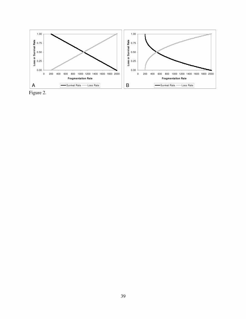
If the survival rate declines as a linear function of the fragmentation rate, then the

function that describes the relationship between the loss rate and the fragmentation rate would be

Lij = σ × (Fij – βi), (eq. 3)

where σ is a constant that determines the slope of the relationship; this constant must have a

value that is positive but very small (i.e., much less than one) for any specimens to remain

identifiable at most levels of fragmentation. A “loss function” of this sort and its corresponding

“survival function” are illustrated in Figure 2A. Linear relationships like those in Figure 2A are

10

the simplest possible relationships that can be assumed, but the experiment that I discuss below

suggests that such relationships are unrealistic. Rather, in that experiment, the survival rate first

begins to decline steeply as the fragmentation rate increases and then levels off somewhat at

higher fragmentation rates. Figure 2B presents a survival function of this sort along with its

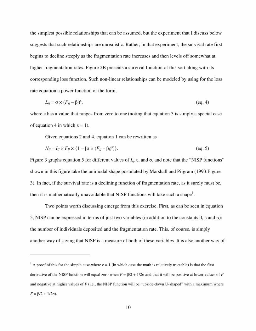
corresponding loss function. Such non-linear relationships can be modeled by using for the loss

rate equation a power function of the form,

Lij = σ × (Fij – βi)ε, (eq. 4)

where ε has a value that ranges from zero to one (noting that equation 3 is simply a special case

of equation 4 in which ε = 1).

Given equations 2 and 4, equation 1 can be rewritten as

Nij = Iij × Fij × {1 – [σ × (Fij – βi)ε]}. (eq. 5)

Figure 3 graphs equation 5 for different values of Iij, ε, and σ, and note that the “NISP functions”

shown in this figure take the unimodal shape postulated by Marshall and Pilgram (1993:Figure

3). In fact, if the survival rate is a declining function of fragmentation rate, as it surely must be,

then it is mathematically unavoidable that NISP functions will take such a shape1.

Two points worth discussing emerge from this exercise. First, as can be seen in equation

5, NISP can be expressed in terms of just two variables (in addition to the constants β, ε and σ):

the number of individuals deposited and the fragmentation rate. This, of course, is simply

another way of saying that NISP is a measure of both of these variables. It is also another way of

1 A proof of this for the simple case where ε = 1 (in which case the math is relatively tractable) is that the first

derivative of the NISP function will equal zero when F = β/2 + 1/2σ and that it will be positive at lower values of F

and negative at higher values of F (i.e., the NISP function will be “upside-down U-shaped” with a maximum where

F = β/2 + 1/2σ).

11

saying that, for the large number of archaeological research questions that require us to measure

something along the lines of the number of individual animals deposited, fragmentation is a

potential confounding variable whose effects must be controlled.

It remains to be determined, however, precisely how much error fragmentation might

introduce into analyses of taxonomic abundance that use NISP, which leads to the second point.

As can be seen in Figure 3, which presents simulated NISP functions based on the survival and

loss functions shown in Figure 2, the degree to which NISP will be affected by fragmentation

depends on the shape of the survival function. The values of I and β are identical in Figures 3A

and 3B, and in both figures loss becomes complete at approximately the same fragmentation rate.

The sole difference between the two figures is that the NISP functions in Figure 3A are based on

a linear survival function (Figure 2A), whereas those in Figure 3B are based on a non-linear

survival function in which survival initially declines steeply and then levels off somewhat

(Figure 2B). Because of this difference in survival function, the maximum NISP values reached

in Figure 3B are much lower than (in fact, approximately half the size of) the maximum NISP

values reached in Figure 3A. Obviously, we would be much better off if, in the real world, NISP

behaved more like it does in Figure 3B than it does in Figure 3A: “flatter” NISP functions would

mean that differences in fragmentation rates would lead to smaller differences in NISP values,

and we could be more confident that variability in NISP values truly reflected variability in

taxonomic abundance rather than simply variability in rates of fragmentation.

I next present the results of an experiment designed to further explore the NISP model

presented here. These experimental results can be used to a certain extent to draw inferences

about the degree to which NISP values are likely to be affected by fragmentation rates in the real

world. More important, the experiment provides an evaluation of methods that might be used to

12

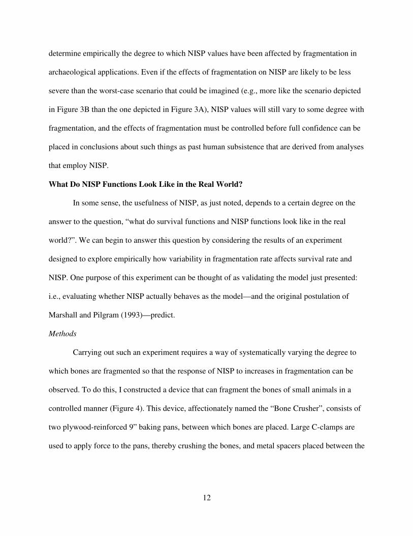
determine empirically the degree to which NISP values have been affected by fragmentation in

archaeological applications. Even if the effects of fragmentation on NISP are likely to be less

severe than the worst-case scenario that could be imagined (e.g., more like the scenario depicted

in Figure 3B than the one depicted in Figure 3A), NISP values will still vary to some degree with

fragmentation, and the effects of fragmentation must be controlled before full confidence can be

placed in conclusions about such things as past human subsistence that are derived from analyses

that employ NISP.

What Do NISP Functions Look Like in the Real World?

In some sense, the usefulness of NISP, as just noted, depends to a certain degree on the

answer to the question, “what do survival functions and NISP functions look like in the real

world?”. We can begin to answer this question by considering the results of an experiment

designed to explore empirically how variability in fragmentation rate affects survival rate and

NISP. One purpose of this experiment can be thought of as validating the model just presented:

i.e., evaluating whether NISP actually behaves as the model—and the original postulation of

Marshall and Pilgram (1993)—predict.

Methods

Carrying out such an experiment requires a way of systematically varying the degree to

which bones are fragmented so that the response of NISP to increases in fragmentation can be

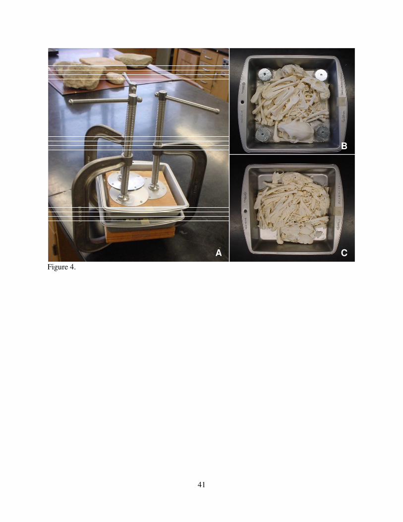
observed. To do this, I constructed a device that can fragment the bones of small animals in a

controlled manner (Figure 4). This device, affectionately named the “Bone Crusher”, consists of

two plywood-reinforced 9” baking pans, between which bones are placed. Large C-clamps are

used to apply force to the pans, thereby crushing the bones, and metal spacers placed between the

13

pans limit the degree to which the bones are fragmented. By progressively reducing the size of

the spacers, the fragmentation rate can be progressively increased.

The experiment described here used the skeletons of two domestic rabbits (Oryctolagus

cuniculus) and one domestic cat (Felis domesticus). The skeletons of two different taxa were

used and were mixed together so that the analyst would be placed in a realistic position of having

to make taxonomic identifications based on osteological characteristics: this would not be the

case if all specimens were from a single taxon because the taxon of each specimen would be

known a priori. However, because it was necessary to do this, fragmentation rates and survival

rates cannot be calculated for each taxon individually in the experiment: unidentified specimens

are included in the calculation of these variables, and the unidentified specimens from the mixed-

taxon samples, by definition, cannot be attributed to one taxon or the other.

The skeletons were purchased from commercial suppliers so that the bones would be as

complete as possible and so that they would be uniform in color (bleached white), thereby

precluding the possibility that specimens might be identified to taxon based on color rather than

on osteology. Likewise, two taxa of roughly similar body size were used so that size-related

characteristics (e.g., cortical bone thickness) would not provide clues for taxonomic

identification. The complete skeletons were used with the exception of these elements: vertebrae,

ribs, sternebrae, clavicles, carpals, tarsals other than the astragalus and calcaneus, and second and

third phalanges. The same three skeletons were used in each round of the experiment, and bones

were identified by a single analyst (the author) using the standard zooarchaeological procedure

of comparison with reference skeletons.

The experiment was conducted in a series of “rounds”. In each round, bones were

fragmented in the Bone Crusher to a degree that was determined by the spacer height. The

14

specimens were then screened through nested geological sieves using a Ro-Tap electric sieve

shaker to mimic archaeological recovery techniques (with the time and intensity of shaking held

constant for each round), the specimens from each screen size fraction were identified and

counted, and the process was then repeated in the next round using a shorter spacer that allowed

for greater fragmentation. Seven rounds of bone crushing were conducted, a number that was

sufficient for evaluating the model presented above. Data were also collected at “round 0” for the

unfragmented skeletons prior to any crushing. In addition to the taxonomic identification of each

specimen (“rabbit”, “cat”, or “unidentified”), several other variables were also recorded at each

round, and these are described below with discussions of methods as appropriate.

Sieve mesh sizes used were 1/4” (6.4 mm), 1/8” (3.2 mm), and 2 mm. All specimens

retained in each of these mesh sizes were counted and identified after each round, while material

that fell through the 2 mm screen was captured and weighed but not counted. Thus, in discussing

the experiment results, the term “specimen” refers to any piece of bone, identifiable or

unidentifiable, that was retained in the 2 mm or larger screen. The data on identified specimens

that are presented below are for specimens retained in 1/8” or larger screens (i.e., for specimens

from both the 1/8” and 1/4” screen fractions). This keeps these data relevant to what may be the

smallest screen size commonly used for large-scale recovery of archaeofaunal remains. Because

nested screens were used, data from the experiment could be used to explore interactions

between NISP functions and variability in screen size (relating the variable of survival rate used

in this paper to the variable of “recovery rate” used in the model of screen size effects discussed

in Cannon 1999), but that is not done here so that the focus of this paper can be kept on the

relationship between NISP and fragmentation.

15

Results

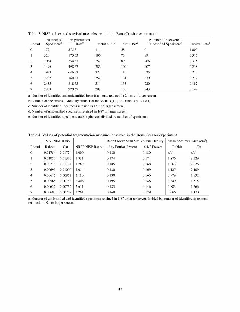
Data from this experiment that are relevant to evaluating the model discussed above are

presented in Table 3. Importantly, the experiment provides empirical support for the hypothesis

that NISP values should first rise at lower levels of fragmentation and then decline at higher

levels. Figure 5 depicts the NISP functions that resulted from the experiment for both rabbit and

cat specimens: the functions for both taxa take the unimodal shape that to this point has remained

hypothetical in zooarchaeology.

Maximum NISP values observed in the experiment are approximately 3.1 times and 2.3

times the starting whole bone values for rabbit and cat, respectively (352/114 for rabbit and

133/58 for cat). These maximum NISP values occur in rounds 5 and 6, where the fragmentation

rate is, respectively, 13.3 times and 14.3 times the starting value for whole bones (760.67/57.33

for round 5 and 818.33/57.33 for round 6). In other words, the decline in specimen survivorship

evidently overtakes the increase in specimen production at around a level of fragmentation that

equates to each bone being broken, on average, into about 13 or 14 pieces, and NISP declines

beyond that level of fragmentation. Of course, the values discussed here are specific to the taxa

and elements, mode of fragmentation (mechanical crushing), post-depositional taphonomic

history (none), recovery method (1/8” screen), and zooarchaeological analyst involved in this

experiment, and they are likely not generalizable on an absolute scale to other sets of conditions.

They may, however, provide at least an order-of-magnitude scale indication of the degree to

which NISP values might be inflated by fragmentation, as well as the level of fragmentation at

which that inflation will be the greatest.

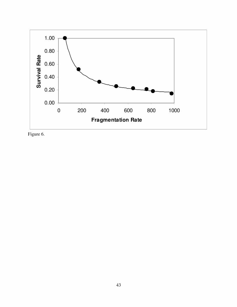
Also importantly, the experiment produced a survival function that is decidedly non-

linear, as is illustrated in Figure 6 (and again, as was noted above, this survival function is not

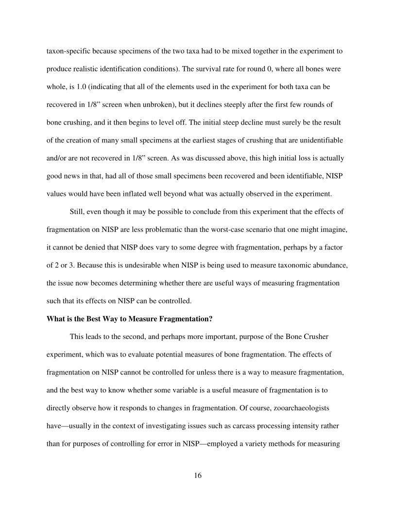
16

taxon-specific because specimens of the two taxa had to be mixed together in the experiment to

produce realistic identification conditions). The survival rate for round 0, where all bones were

whole, is 1.0 (indicating that all of the elements used in the experiment for both taxa can be

recovered in 1/8” screen when unbroken), but it declines steeply after the first few rounds of

bone crushing, and it then begins to level off. The initial steep decline must surely be the result

of the creation of many small specimens at the earliest stages of crushing that are unidentifiable

and/or are not recovered in 1/8” screen. As was discussed above, this high initial loss is actually

good news in that, had all of those small specimens been recovered and been identifiable, NISP

values would have been inflated well beyond what was actually observed in the experiment.

Still, even though it may be possible to conclude from this experiment that the effects of

fragmentation on NISP are less problematic than the worst-case scenario that one might imagine,

it cannot be denied that NISP does vary to some degree with fragmentation, perhaps by a factor

of 2 or 3. Because this is undesirable when NISP is being used to measure taxonomic abundance,

the issue now becomes determining whether there are useful ways of measuring fragmentation

such that its effects on NISP can be controlled.

What is the Best Way to Measure Fragmentation?

This leads to the second, and perhaps more important, purpose of the Bone Crusher

experiment, which was to evaluate potential measures of bone fragmentation. The effects of

fragmentation on NISP cannot be controlled for unless there is a way to measure fragmentation,

and the best way to know whether some variable is a useful measure of fragmentation is to

directly observe how it responds to changes in fragmentation. Of course, zooarchaeologists

have—usually in the context of investigating issues such as carcass processing intensity rather

than for purposes of controlling for error in NISP—employed a variety methods for measuring

17

bone fragmentation (see Wolverton et al. 2008 and references therein; also see Ugan 2005).

However, the justification for the use of these methods typically relies more on logical argument

than on direct empirical evaluation. Direct empirical evaluation can be carried out for certain

potential fragmentation measures using data from the Bone Crusher experiment.

The variables considered here consist of three that have been used as fragmentation

measures in previous zooarchaeological research, and one that has not to my knowledge been so

used but that conceivably might be. They are the ratio of MNI to NISP, the ratio of the total

number of recovered specimens to NISP, bone density, and average specimen size. Each of these

is discussed next in turn. Data from the Bone Crusher experiment that are relevant to evaluating

these potential fragmentation measures are presented in Table 4.

MNI:NISP Ratio

The first measure of fragmentation that can be evaluated using data from the Bone

Crusher experiment is the ratio of MNI to NISP. This ratio or the fundamentally similar

MNE:NISP ratio (or the inverse NISP:MNI ratio or NISP:MNE ratio) has been used as a

measure of fragmentation in previous zooarchaeological applications focused on exploring

carcass processing intensity (e.g., Wolverton 2002; Wolverton et al. 2008; Ugan 2005). The logic

behind the use of this variable is essentially that NISP should increase with greater

fragmentation, whereas MNI or MNE should not (see Marshall and Pilgram 1993). Thus, a

negative relationship should be observed between MNI:NISP ratio and degree of bone

fragmentation. As Wolverton (2002; Wolverton et al. 2008) points out, however, such a

relationship should hold only up to a point; citing the observation of Marshall and Pilgram

(1993) that NISP should eventually begin to decline at high rates of fragmentation, he notes that

ratios like MNI:NISP should also eventually exhibit reversals at high rates of fragmentation. This

18

would limit the utility of ratios like MNI:NISP as fragmentation measures because it would mean

that a single ratio value could indicate two very different levels of fragmentation.

The Bone Crusher experiment provides empirical support for the suggestion that such

ratios will, in fact, behave in this fashion (Table 4). Specifically, as NISP starts to decline at

higher levels of fragmentation in the experimental results, MNI does not, and this causes the

MNI:NISP ratio to reverse direction along with NISP, as is illustrated in Figure 7. This suggests

that ratios like MNI:NISP do indeed provide an ambiguous measure of fragmentation.

NRSP:NISP Ratio

Noting that ratios such as MNI:NISP may vary with fragmentation in the problematic

manner just demonstrated, Wolverton (2002; Wolverton et al. 2008) supplements the use of such

ratios with another ratio—used earlier by Grayson (1991)—that he refers to as the ratio of the

number of specimens (NSP) to NISP. This is simply the total number of specimens in an

assemblage —identified and unidentified—divided by NISP (or, it is the inverse of the

proportion of the specimens in an assemblage that are identifiable). Here, I evaluate the utility of

this variable as a measure of bone fragmentation, though I note that, strictly speaking, the

variable that is being used here is the number of recovered specimens, not the number of

specimens that may actually have been produced (i.e., not the “number of specimens” as this

term is defined in the model presented above). Obviously, many of the fragments into which a

carcass was broken over the course of its taphonomic history may go unrecovered due to such

factors as post-depositional attrition or archaeological recovery methods, and it is only the subset

of the fragments that are actually recovered that can be used in a fragmentation measure. I refer

to this subset here by the abbreviation NRSP, for number of recovered specimens.

19

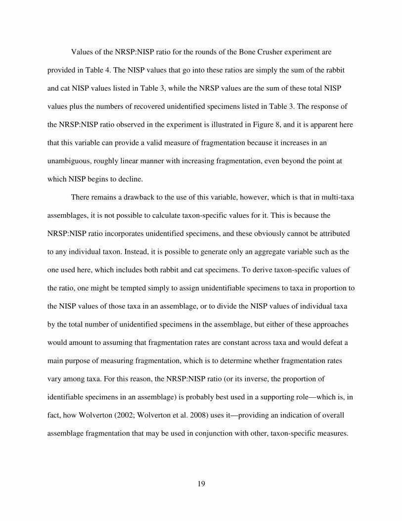
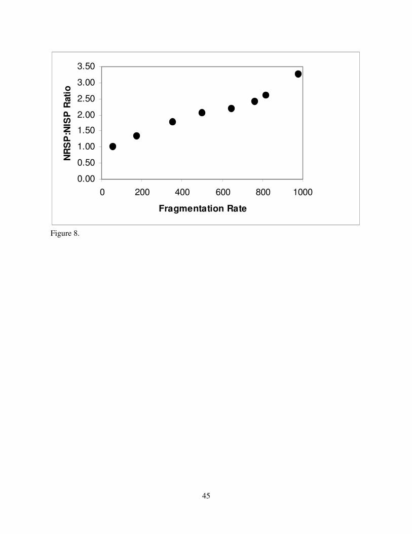
Values of the NRSP:NISP ratio for the rounds of the Bone Crusher experiment are

provided in Table 4. The NISP values that go into these ratios are simply the sum of the rabbit

and cat NISP values listed in Table 3, while the NRSP values are the sum of these total NISP

values plus the numbers of recovered unidentified specimens listed in Table 3. The response of

the NRSP:NISP ratio observed in the experiment is illustrated in Figure 8, and it is apparent here

that this variable can provide a valid measure of fragmentation because it increases in an

unambiguous, roughly linear manner with increasing fragmentation, even beyond the point at

which NISP begins to decline.

There remains a drawback to the use of this variable, however, which is that in multi-taxa

assemblages, it is not possible to calculate taxon-specific values for it. This is because the

NRSP:NISP ratio incorporates unidentified specimens, and these obviously cannot be attributed

to any individual taxon. Instead, it is possible to generate only an aggregate variable such as the

one used here, which includes both rabbit and cat specimens. To derive taxon-specific values of

the ratio, one might be tempted simply to assign unidentifiable specimens to taxa in proportion to

the NISP values of those taxa in an assemblage, or to divide the NISP values of individual taxa

by the total number of unidentified specimens in the assemblage, but either of these approaches

would amount to assuming that fragmentation rates are constant across taxa and would defeat a

main purpose of measuring fragmentation, which is to determine whether fragmentation rates

vary among taxa. For this reason, the NRSP:NISP ratio (or its inverse, the proportion of

identifiable specimens in an assemblage) is probably best used in a supporting role—which is, in

fact, how Wolverton (2002; Wolverton et al. 2008) uses it—providing an indication of overall

assemblage fragmentation that may be used in conjunction with other, taxon-specific measures.

20

Bone Density

Another potential measure of fragmentation that can be evaluated here is bone density.

(Bone density scan site proportion, which I have used previously as a fragmentation measure—as

in the analysis presented at the start of this paper—is not evaluated here because the measure

discussed next clearly superior to this in its ease of use.) I am not aware of any zooarchaeological

application where analyses based on bone density have been used to measure fragmentation per

se, but bone density is, of course, very commonly used as a general indicator of attrition in faunal

assemblages (see overview in Lyman 1994). Because attrition may just be another way of saying

loss of identifiable specimens, and because, as I argued earlier, loss of identifiable specimens

should be related in a predictable manner to fragmentation, it is plausible that bone density data

might provide a useful measure of fragmentation. More specifically, if the assumptions that

underlie typical thinking about density-mediated attrition are correct, then it should be expected

that denser portions of skeletal elements would be more likely to survive processes that produce

fragmentation. In turn, if this were the case, the average density of the identifiable specimens

within an assemblage would increase with greater fragmentation.

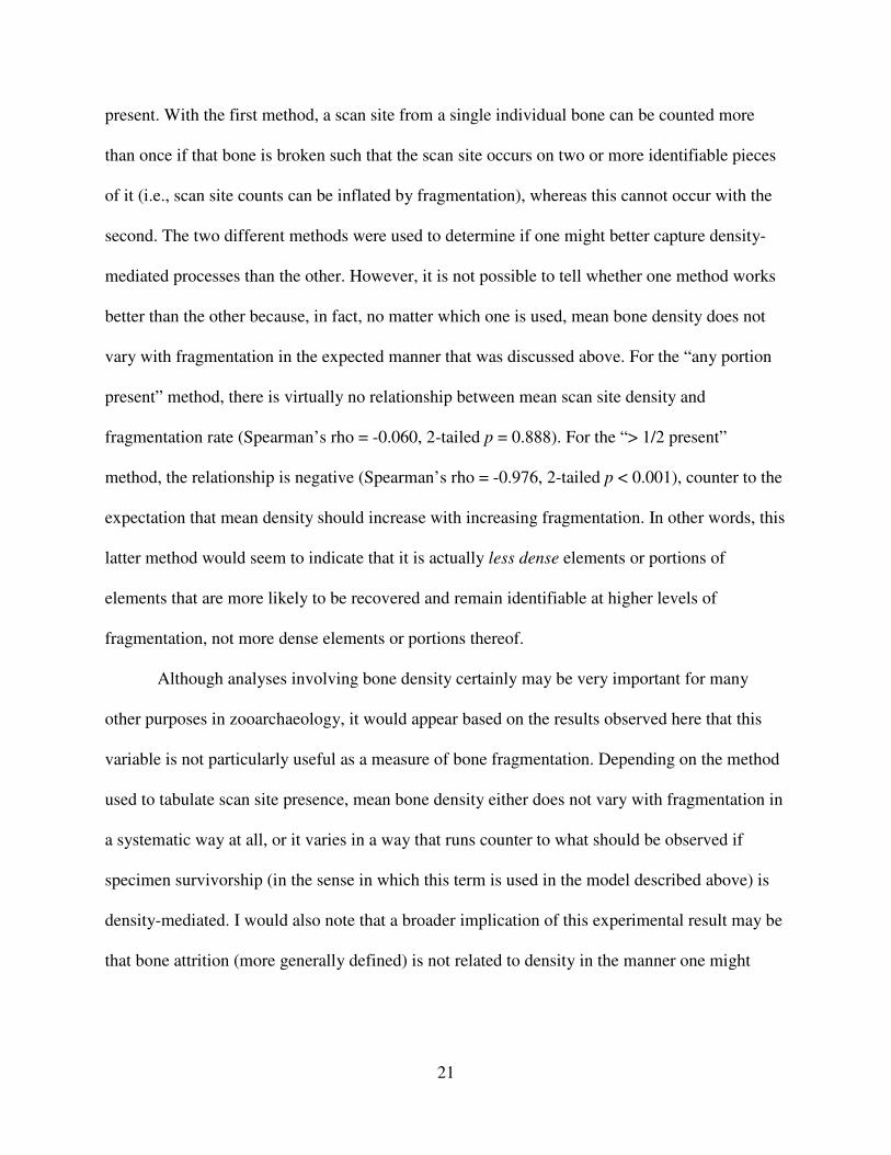
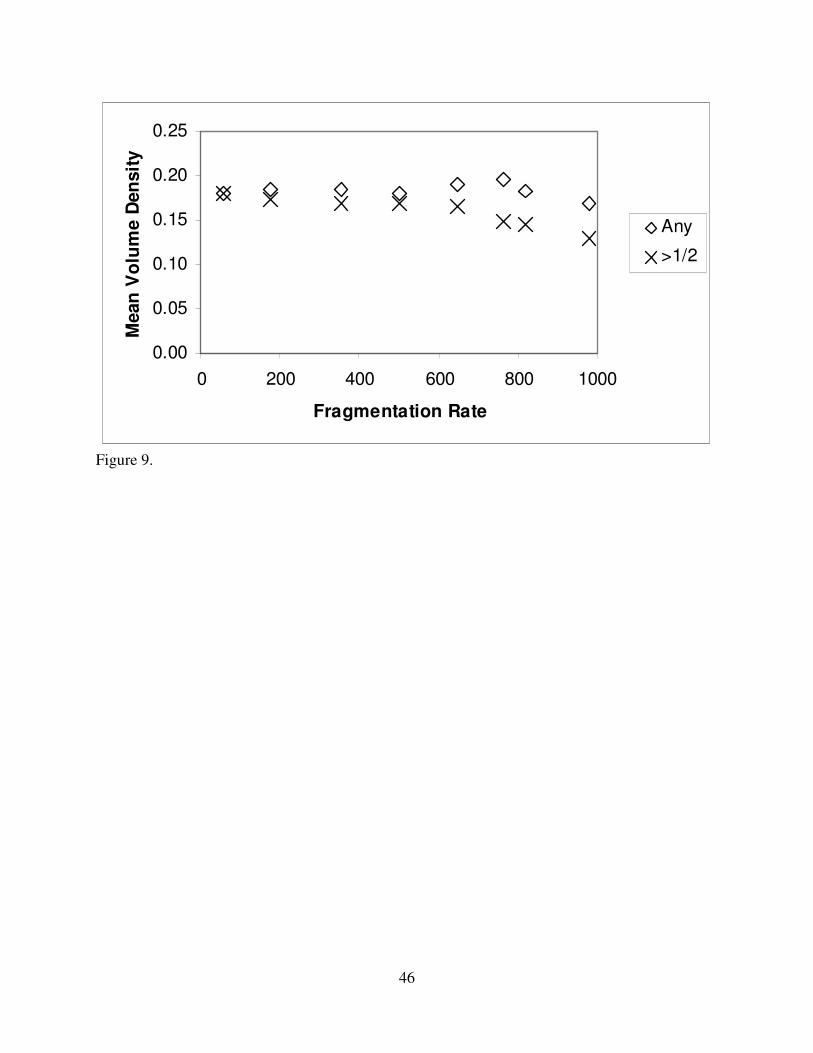
While this seems reasonable as an expectation, it is not borne out empirically by the Bone

Crusher experiment. Data relevant to this test are provided in Table 4 and graphed in Figure 9.

The data in this table and figure reflect the mean volume density of all scan sites present on

identified rabbit specimens (again, from 1/8” and larger screens) using the rabbit bone density

measurements of Pavao and Stahl (1999). Scan site “presence” was recorded in this experiment

in each of two different ways: in the first method a scan site was recorded as present if any

portion of the bone at the location of that scan site was present, and in the second a scan site was

recorded as present only if at least half of the circumference of the bone at that location was

21

present. With the first method, a scan site from a single individual bone can be counted more

than once if that bone is broken such that the scan site occurs on two or more identifiable pieces

of it (i.e., scan site counts can be inflated by fragmentation), whereas this cannot occur with the

second. The two different methods were used to determine if one might better capture density-

mediated processes than the other. However, it is not possible to tell whether one method works

better than the other because, in fact, no matter which one is used, mean bone density does not

vary with fragmentation in the expected manner that was discussed above. For the “any portion

present” method, there is virtually no relationship between mean scan site density and

fragmentation rate (Spearman’s rho = -0.060, 2-tailed p = 0.888). For the “> 1/2 present”

method, the relationship is negative (Spearman’s rho = -0.976, 2-tailed p < 0.001), counter to the

expectation that mean density should increase with increasing fragmentation. In other words, this

latter method would seem to indicate that it is actually less dense elements or portions of

elements that are more likely to be recovered and remain identifiable at higher levels of

fragmentation, not more dense elements or portions thereof.

Although analyses involving bone density certainly may be very important for many

other purposes in zooarchaeology, it would appear based on the results observed here that this

variable is not particularly useful as a measure of bone fragmentation. Depending on the method

used to tabulate scan site presence, mean bone density either does not vary with fragmentation in

a systematic way at all, or it varies in a way that runs counter to what should be observed if

specimen survivorship (in the sense in which this term is used in the model described above) is

density-mediated. I would also note that a broader implication of this experimental result may be

that bone attrition (more generally defined) is not related to density in the manner one might

22

expect, at least when attrition occurs solely through mechanical crushing as was the case in this

experiment; however, further exploration of that issue is beyond the scope of the present paper.

Specimen Size

A final potential useful measure of fragmentation that I consider here is specimen size.

Specimen size is directly and obviously related to fragmentation because, as a given set of bones

becomes broken up into more and more pieces, the average size of those pieces must necessarily

decrease. However, a potentially serious practical drawback to using this variable as a measure

of fragmentation is the time that it takes to record it using traditional methods (e.g., manually

measuring individual specimens one at a time using calipers, a size template, etc.). Although

specimen size often is measured manually in zooarchaeological analyses—including for

purposes of measuring bone fragmentation (e.g., Ugan 2005)—time and budget constraints make

it impractical to do this in some projects, and even when such constraints do not completely

preclude manual measurement, the labor required invariably makes it very expensive.

Fortunately, though, there is a method available for measuring specimen size that enables large

numbers of bone fragments to be measured very quickly and cheaply, greatly easing the

constraints on size measurement. This method involves the use of digital image analysis.

A particular focus of the Bone Crusher experiment was to employ digital image analysis

to track changes in specimen size across experimental rounds, and data from the experiment can

therefore be used to evaluate whether specimen size—and specifically specimen size as

measured through digital image analysis—provides a useful measure of bone fragmentation. To

perform the digital image analysis, digital photographs of the experimental assemblage were

taken at the end of every round of the experiment, and these were analyzed using ImageJ

software, which is freely available online through the U.S. National Institutes of Health

23

(http://rsb.info.nih.gov/ij/index.html). Among many other things, this software package can

automatically trace outlines of objects in a digital image, calculate the area within those outlines

(calibrated based on some spatial reference in the photo), and output a file with size

measurements for each object in the image (Figure 10). Arranging bones to take the photographs

requires some time—specimens must be laid out so that none are touching—as does the image

analysis process, but this is only a very small fraction of what would be necessary to manually

take size measurements on individual specimens.

Methods: At a more detailed level, the methods used for digital image analysis were as

follows. After each round of bone crushing and identification, photographs were taken separately

by taxon (rabbit, cat, and unidentified) and by screen size fraction (an exception was that taxon-

specific photographs were not taken for whole bones at round 0 of the experiment because the

utility of such photographs was not recognized until after round 1 crushing had occurred). This

was done to enable calculation of taxon- and screen size-specific average size values. The size

data reported here (Table 4) are for identified rabbit and cat specimens from 1/8” screen samples

(i.e., from the 1/8” and 1/4” screen fractions combined). Although ImageJ will compute many

shape- and size-related variables for objects in an image, simple specimen area was used for this

analysis. Because area is a two-dimensional variable and bone fragments are three-dimensional,

some error will be present in the size measurements that is related to variation in the orientation

of individual objects: e.g., a bone that is long and flat will be measured as having a much smaller

area if it is lying on its edge in a photograph than would be the case if it were lying flat. In an

effort to randomize such error, the specimens in each sub-assemblage (i.e., from each taxon and

screen size fraction) were photographed three times at each round of the experiment, and the

24

specimens were shuffled between photographs to vary their orientations. The data used here are

based on averages of the three “shuffles” for each sub-assemblage.

The photographs were taken with a Sony Cyber-shot 1.3 megapixel digital camera

(though any basic digital camera will suffice). The camera was mounted to a copy stand for ease

of use and consistency among photographs, and a black background was used for maximum

contrast with the white bones. The photographs, which were taken in color and saved as .jpg

files, were opened in ImageJ and analyzed using the software’s “Analyze Particles” tool. Prior to

analysis, the photographs were converted to black-and-white 8-bit image type within the

software, which is a prerequisite for use of the Analyze Particles tool, and image threshold

values were set to 100 (lower) and 255 (upper) to further maximize contrast. In addition, the

distance scale was calibrated using the software’s “Set Scale” tool and based on a 10-cm scale

bar that was place in each photograph for distance calibration purposes (see Figure 10). Labels

denoting the experimental round, screen size, taxon, and shuffle were also placed in each

photograph for record-keeping purposes; these labels and the scale bar were excluded from the

analyzed image using the software’s “Select” function before running Analyze Particles.

ImageJ outputs analysis results for an image as a text file that includes (among several

other variables) an area measurement for each object in the image. The text files for each

analyzed image were pasted into a single master spreadsheet for subsequent analysis. In addition,

the “Show Outlines” option of the Analyze Particles tool was selected for the analysis of each

image; this produced jpgs showing outlines of the objects in each image (see Figure 10B), which

were saved, again for record-keeping purposes. Very small particles (even pieces of dust), which

unavoidably appear in photographs, are measured by the software and included in the output, but

25

these are easily recognized by their extremely small area values and were deleted from the

master data file for this analysis.

Results: The results of the Bone Crusher experiment indicate that specimen size—and

specifically specimen area as measured through digital image analysis—is a valid and useful

measure of fragmentation. For both rabbit and cat specimens, size declines in a roughly linear

manner with increasing fragmentation (Figure 11). The fact that the relationship is linear means

that specimen size is more useful as a measure of fragmentation than MNI:NISP ratio, which can

give ambiguous results due to non-linear responses to increasing fragmentation. In addition, the

fact that it exhibits any sort of predictable relationship with fragmentation at all makes specimen

size more useful than average bone density, which either does not vary systematically with

fragmentation or varies in a manner that runs counter to what would be expected if specimen

survivorship were density-mediated. And finally, unlike the NRSP:NISP ratio, it is possible to

generate taxon-specific values for specimen size through digital image analysis, as long as

specimens are grouped by taxon in the images used in the analysis.

Discussion

This paper has presented a formal model of the relationship between NISP and bone

fragmentation that can enable a more detailed understanding of that relationship than previous,

primarily verbal (though important) explorations of it are able to. It has also presented the results

of an experiment that provide empirical support for the oft-discussed, but never tested,

hypothesis that NISP values should first increase and then decrease with increases in

fragmentation rate. The experimental results also suggest that NISP values may not be inflated

by fragmentation as much as some might fear, perhaps only by a factor of about 2 or 3 relative to

unfragmented, whole bone values. And finally, and perhaps most important, the experimental

26

results provide empirical evaluation of several potential measures of bone fragmentation,

suggesting that specimen size—which can be determined easily through digital image analysis—

is more useful than other variables that have been or that might be used as fragmentation

measures. Neither MNI:NISP ratio or mean bone density appear to vary with fragmentation in

ways that make them useful measures of it, and while NRSP:NISP ratio does, it is not possible to

generate taxon-specific values of this ratio in multi-taxa assemblages. Specimen size, on the

other hand, varies with fragmentation rate linearly, providing an unambiguous measure of it, and

it can be calculated for individual taxa. Moreover, it can be measured fairly quickly and easily,

even for large assemblages, through digital image analysis.

There are, of course, other variables not considered here that might also provide useful

measures of bone fragmentation. For example, average specimen weight has been used (e.g.,

Ugan 2005), and this variable should be related to fragmentation rate in a direct and

unambiguous manner much as average specimen size is. I would note, however, that bone weight

may be affected by post-depositional diagenesis, as well as by processes that result in density

mediated attrition: assemblages that have experienced more density-mediated attrition will

necessarily be biased towards greater average mass per specimen volume (i.e., size). Still, in

cases where it can independently be demonstrated that diagenesis or density-mediated attrition

have not substantially affected bone samples differentially, weight may provide a useful way of

comparing the degree of fragmentation among those samples.

There are also, of course, many types of research questions other than the kind on which I

have focused here for which it is necessary to be able to measure bone fragmentation. Though

this paper has focused on the problem of fragmentation-related error in NISP-based analyses of

taxonomic abundance, fragmentation is probably most often examined within zooarchaeology in

27

the context of questions about carcass-processing intensity, as I noted above (e.g., Wolverton et

al. 2008; Ugan 2005). In analyses focused on questions of that sort, fragmentation does not

constitute a source of error, but is instead the variable of direct interest. The empirical evaluation

of fragmentation measures presented here should be just as useful for bone processing studies as

it is for NISP-based taxonomic abundance studies.

And finally, how, specifically, should a measure of fragmentation be used to control for

the effects of this variable in NISP-based analyses of taxonomic abundance? Simply put, all that

needs to be done is to show that fragmentation does not vary among samples in a manner that

might confound conclusions about taxonomic abundance. In the Mimbres Valley example

discussed at the start of this paper, it appears that fragmentation—in that case measured by mean

scan site proportions—does vary in a way that could provide an alternative explanation to the

artiodactyl resource depression-population rebound hypothesis for the observed pattern in the

Artiodactyl Index. This is cause for concern (though it also certainly raises interesting new

questions regarding the cause of the differences in fragmentation)—and the problem would not

even have been recognized had a fragmentation measure not been applied. If, on the other hand,

it were the case that fragmentation did not vary substantially among those samples, then there

would not be cause for concern and it would be possible to place greater confidence in the

resource depression-population rebound explanation—but the fragmentation analysis would have

to actually be conducted in order for that confidence to be earned. And because it is possible to

quantify fragmentation directly and efficiently through digital image-based measurement of

specimen size, valid reasons for not taking fragmentation into account begin to disappear.

There are, of course, complications to be dealt with in such an approach. In particular, if

average specimen size is the fragmentation measure that is used, then the average size of whole

28

bones of the elements present in the samples being compared would have to be roughly the same

for average specimen size to be a useful measure of fragmentation (and the same point probably

also applies to specimen weight). For example, an analysis could include one sample consisting

entirely of deer scapulae and another consisting entirely of deer phalanges: if both samples were

completely unfragmented, the average deer specimen size would be very different between them,

even though the degree of fragmentation is exactly the same. For this reason, specimen size is

probably best used when it can be shown that skeletal element relative abundance distributions

for a given taxon are roughly identical among the samples being compared—meaning that

unfragmented bone size distributions would have been approximately the same—or perhaps

analysis could be carried out on an element-by-element basis.

Regardless of the complications, however, NISP-based taxonomic abundance analyses

would benefit greatly from the incorporation of the use of a fragmentation measure to assess the

degree to which observed patterns are the result of variability in fragmentation. Once this is

done—and measurement of specimen size through digital image analysis provides a way in

which it can be done easily—we can move on to causes of patterns in NISP that are potentially

much more interesting.

29

Acknowledgements

I am tremendously grateful to Nicci Barger, who provided tireless assistance with the

Bone Crusher experiment and digital image analysis. I also thank the students in my

zooarchaeology course at California State University, Long Beach, who helped with the analysis

of the fauna from the Stailey site, and Carl Lipo, who suggested the use of ImageJ. Finally, I

thank Virginia Butler, Chris Darwent, and Michael O’Brien for their invitation to participate in

the Fryxell symposium in honor of Lee Lyman in which a version of this paper was presented,

and I thank Lee himself for his innumerable, thought-provoking contributions to the field of

zooarchaeology.

30

References Cited

Binford, L. R. (1978). Nunamiut ethnoarchaeology. New York: Academic Press.

Broughton, J. M., Cannon, M. D., Bartelink, E. J. (2010). Evolutionary ecology, resource

depression, and niche construction theory in archaeology: applications to central California

hunter-gatherers and Mimbres-Mogollon agriculturalists. Journal of Archaeological Method and

Theory 4, 371-421.

Broughton, J. M., Cannon, M. D., Bayham, F. E., Byers, D. A. (2011). Prey body size and

ranking in zooarchaeology: theory, empirical evidence, and applications from the northeastern

Great Basin. American Antiquity 76, 403-428.

Cannon, M. D. (1999). A mathematical model of the effects of screen size on zooarchaeological

relative abundance measures. Journal of Archaeological Science 26, 205-214.

Cannon, M. D. (2001). Large mammal resource depression and agricultural intensification: an

empirical test in the Mimbres Valley, New Mexico. Ph.D. Dissertation, Department of

Anthropology, University of Washington, Seattle.

Cannon, M. D. (2003). A model of central place forager prey choice and an application to faunal

remains from the Mimbres Valley, New Mexico. Journal of Anthropological Archaeology 22, 1-

25.

31

Grayson, D. K. (1984). Quantitative zooarchaeology. New York: Academic Press.

Grayson, D. K. (1991). Alpine faunas from the White Mountains, California: adaptive change in

the prehistoric Great Basin? Journal of Archaeological Science 18, 483-506.

Klein, R. G., & Cruz-Uribe, K. (1984). The analysis of animal bones from archaeological sites.

Chicago: University of Chicago Press.

Lyman, R. L. (1984). Bone density and differential survivorship of fossil classes. Journal of

Anthropological Archaeology 3, 259-299.

Lyman, R. L. (1985). Bone frequencies: differential transport, in situ destruction, and the MGUI.

Journal of Archaeological Science 12, 221-236.

Lyman, R. L. (1994). Vertebrate taphonomy. New York: Cambridge University Press.

Lyman, R. L., & O’Brien, M. J. (1987). Plow-zone zooarchaeology: fragmentation and

identifiability. Journal of Field Archaeology 14, 493-500.

Marshall, F., & Pilgram, T. (1993). NISP vs. MNI in quantification of body-part representation.

American Antiquity 58, 261-269.

32

Nelson, B. A., & LeBlanc, S. A. (1986). Short-term sedentism in the American southwest: the

Mimbres Valley Salado. Albuquerque: University of New Mexico Press.

Pavao, B., & Stahl, P. W. (1999). Structural density assays of leporid skeletal elements with

implications for taphonomic, actualistic, and archaeological research. Journal of Archaeological

Science 26, 53-66.

Rogers, A. R. (2000). Analysis of bone counts by maximum likelihood. Journal of

Archaeological Science 27, 111-125.

Stiner, M. C., Kuhn, S. L., Surovell, T. A., Godlberg, P., Meignen, L., Weiner, S., Bar-Yosef, O.

(2001). Bone preservation in Hayonim Cave (Israel): a macroscopic and mineralogic study.

Journal of Archaeological Science 28, 643–659.

Ugan, A. (2005). Climate, bone density, and resource depression: what is driving variation in

large and small game in Fremont archaeofaunas? Journal of Anthropological Archaeology 24,

227-251.

Watson, J. P. N. (1972). Fragmentation analysis of animal bone samples from archaeological

sites. Archaeometry, 14, 221-228.

White, T. E. (1952). Observations on the butchering technique of some aboriginal peoples: I.

American Antiquity 17, 337-338.

33

White, T. E. (1953). A method of calculating the dietary percentage of various food animals

utilized by aboriginal peoples. American Antiquity 18, 396-398.

Wolverton, S. (2002). NISP:MNE and %whole in analysis of carcass exploitation. North

American Archaeologist 23, 85-100.

Wolverton, S., Nagaoka, L., Densmore, J., Fullerton, B. (2008). White-tailed deer harvest

pressure and within-bone nutrient exploitation during the mid-to-late Holocene in southeast

Texas. Before Farming 2008, 1-23.

34

Table 1. Numbers of identified artiodactyl and lagomorph specimens by time period in faunal samples from

archaeological sites in the Mimbres Valley.

Time Period Artiodactyl NISP Lagomorph NISP Total NISP Artiodactyl Index

Cliff Phase 40 5 45 0.889

Terminal Classic Mimbres Phase 16 52 68 0.235

Classic Mimbres Phase 75 268 343 0.219

Three Circle Phase 45 161 206 0.218

Georgetown/San Francisco Phase 5 5 10 0.500

Early Pithouse Period 17 1 18 0.944

Note: Data for the Early Pithouse period through the Terminal Classic are from the Mattocks, McAnally, and Galaz sites and are

reported in Cannon (2001, 2003; also see Broughton et al. 2010). Data for the Cliff phase are from the Stailey site (Nelson and

LeBlanc 1986) and are previously unpublished.

Table 2. Mean proportion of scan sites present on artiodactyl and lagomorph specimens in faunal samples from

archaeological sites in the Mimbres Valley.

Artiodactyls Lagomorphs

Time Period Mean Scan Site Proportion na SDb Mean Scan Site Proportion na SDb

Cliff Phase 0.14 36 0.19 0.62 5 0.25

Terminal Classic Mimbres Phase 0.45 11 0.38 0.41 46 0.26

Classic Mimbres Phase 0.32 46 0.37 0.40 216 0.26

Three Circle Phase 0.29 30 0.25 0.42 139 0.29

Georgetown/San Francisco Phase 0.25 3 0.14 0.23 5 0.15

Early Pithouse Period 0.34 15 0.49 0.17 1 n/a

a. Number of specimens from elements that have scan sites. These values tend to be smaller than the NISP values for the taxon

(Table 1) because scan sites are not available for all elements.

b. Standard deviation of the proportion of scan sites present.

35

Table 3. NISP values and survival rates observed in the Bone Crusher experiment.

Round

Number of

Specimensa Fragmentation

Rateb Rabbit NISPc Cat NISPc

Number of Recovered

Unidentified Specimensd Survival Ratee

0 172 57.33 114 58 0 1.000

1 520 173.33 196 73 89 0.517

2 1064 354.67 257 89 266 0.325

3 1496 498.67 286 100 407 0.258

4 1939 646.33 325 116 525 0.227

5 2282 760.67 352 131 679 0.212

6 2455 818.33 314 133 720 0.182

7 2939 979.67 287 130 943 0.142

a. Number of identified and unidentified bone fragments retained in 2 mm or larger screen.

b. Number of specimens divided by number of individuals (i.e., 3: 2 rabbits plus 1 cat).

c. Number of identified specimens retained in 1/8” or larger screen.

d. Number of unidentified specimens retained in 1/8” or larger screen.

e. Number of identified specimens (rabbit plus cat) divided by number of specimens.

Table 4. Values of potential fragmentation measures observed in the Bone Crusher experiment.

MNI:NISP Ratio Rabbit Mean Scan Site Volume Density Mean Specimen Area (cm2)

Round Rabbit Cat NRSP:NISP Ratioa Any Portion Present > 1/2 Present Rabbit Cat

0 0.01754 0.01724 1.000 0.180 0.180 n/aa n/aa

1 0.01020 0.01370 1.331 0.184 0.174 1.876 3.229

2 0.00778 0.01124 1.769 0.185 0.168 1.363 2.626

3 0.00699 0.01000 2.054 0.180 0.169 1.125 2.109

4 0.00615 0.00862 2.190 0.190 0.166 0.979 1.832

5 0.00568 0.00763 2.406 0.195 0.148 0.849 1.515

6 0.00637 0.00752 2.611 0.183 0.146 0.883 1.566

7 0.00697 0.00769 3.261 0.168 0.129 0.666 1.170

a. Number of unidentified and identified specimens retained in 1/8” or larger screen divided by number of identified specimens

retained in 1/8” or larger screen.

36

Figure Captions

Figure 1. Hypothetical relationship between fragmentation and NISP, after Marshall and Pilgram

(1993).

Figure 2. Simulated linear (A) and non-linear (B) relationships between fragmentation rate and

survival rate (“survival functions”) and between fragmentation rate and loss rate (“loss

functions”) based on equations 2 and 4 in the text. In both figures, β = 200. In A, ε = 1.0 and σ =

0.00056, and in B, ε = 0.4 and σ = 0.05.

Figure 3. Simulated relationships between fragmentation rate and NISP (“NISP functions”)

based on equation 5 in the text. Each graph depicts two taxa that differ in the number of

individuals originally deposited (I): for Taxon 1, I = 20, and for Taxon 2, I = 10. The NISP

functions in A are based on the linear survival function shown in Figure 2A, and those in B are

based on the non-linear survival function shown in Figure 2B.

Figure 4. The “Bone Crusher” (A), showing unfragmented rabbit and cat skeletons before the

first round of crushing with spacers in place (B), and fragmented skeletons after the first round of

crushing (C).

Figure 5. NISP functions observed in the Bone Crusher experiment (polynomial curves are fit to

the observed data points).

37

Figure 6. Survival function observed in the Bone Crusher experiment (a power curve is fit to the

observed data points).

Figure 7. Response of MNI:NISP ratios to increasing fragmentation rates in the Bone Crusher

experiment (polynomial curves are fit to the observed data points).

Figure 8. Response of NRSP:NISP ratio to increasing fragmentation rates in the Bone Crusher

experiment.

Figure 9. Response of identified rabbit specimen mean scan site volume density to increasing

fragmentation rates in the Bone Crusher experiment.

Figure 10. Photograph used as input for ImageJ software (A), and drawing created from this

photograph by ImageJ for particle size and shape analysis (B). Bones shown here are identified

rabbit specimens from the 1/4” screen fraction after round 1 of the Bone Crusher experiment.

Figure 11. Response of mean specimen area to increasing fragmentation rates in the Bone

Crusher experiment.

38

Figure 1.

Degree of Bone Fragmentation

Ab

un

dan

ce E

sti

mate

NISP

39

Figure 2.

0.00

0.25

0.50

0.75

1.00

0 200 400 600 800 1000 1200 1400 1600 1800 2000

Fragmentation Rate

Lo

ss

or

Su

rviv

al

Ra

te

Survival Rate Loss Rate

0.00

0.25

0.50

0.75

1.00

0 200 400 600 800 1000 1200 1400 1600 1800 2000

Fragmentation Rate

Lo

ss

or

Su

rviv

al

Ra

te

Survival Rate Loss RateA B

40

Figure 3.

0

2000

4000

6000

8000

10000

12000

0 200 400 600 800 1000 1200 1400 1600 1800 2000

Fragmentation Rate

NIS

P

Taxon 1 (I = 20) Taxon 2 (I = 10)

0

2000

4000

6000

8000

10000

12000

0 200 400 600 800 1000 1200 1400 1600 1800 2000

Fragmentation Rate

NIS

P

Taxon 1 (I = 20) Taxon 2 (I = 10)A B

41

Figure 4.

A

B

C

42

Figure 5.

0

50

100

150

200

250

300

350

400

0 200 400 600 800 1000

Fragmentation Rate

NIS

P Rabbit

Cat

43

Figure 6.

0.00

0.20

0.40

0.60

0.80

1.00

0 200 400 600 800 1000

Fragmentation Rate

Su

rviv

al

Rate

44

Figure 7.

0.000

0.005

0.010

0.015

0.020

0 200 400 600 800 1000

Fragmentation Rate

MN

I:N

ISP

Rati

o

Rabbit

Cat

45

Figure 8.

0.00

0.50

1.00

1.50

2.00

2.50

3.00

3.50

0 200 400 600 800 1000

Fragmentation Rate

NR

SP

:NIS

P R

ati

o

46

Figure 9.

0.00

0.05

0.10

0.15

0.20

0.25

0 200 400 600 800 1000

Fragmentation Rate

Mean

Vo

lum

e D

en

sit

y

Any

>1/2

47

Figure 10.

A B

48

Figure 11.

0.00

0.50

1.00

1.50

2.00

2.50

3.00

3.50

0 200 400 600 800 1000

Fragmentation Rate

Mean

Sp

ecim

en

Are

a (

sq

. cm

)

Rabbit

Cat