nist database for the simulation of electron spectra for ... · nist database for the simulation of...

NIST Standard Reference Database 100

______________________________________________________________________

NIST Database for the Simulation of Electron Spectra for Surface Analysis (SESSA)

Version 2.0

Users' Guide ______________________________________________________________________ Prepared by: Wolfgang S. M. Werner and Werner Smekal Institute of Applied Physics, Vienna University of Technology, Wiedner Hauptstrasse 8-10, A-1040 Vienna, Austria and Cedric J. Powell Materials Measurement Science Division National Institute of Standards and Technology Gaithersburg, Maryland 20899 October, 2014 U.S. Department of Commerce National Institute of Standards and Technology Measurement Services Division Gaithersburg, Maryland 20899

ii

The National Institute of Standards and Technology (NIST) uses its best efforts to deliver a high quality copy of the database and to verify that the data contained therein have been selected on the basis of sound scientific judgment. However, NIST makes no warranties to that effect, and NIST shall not be liable for any damage that may result from errors or omissions in the database. For a literature citation, the database should be viewed as a book published by NIST. The citation would therefore be: W.S.M. Werner, W. Smekal, and C. J. Powell, NIST Database for the Simulation of Electron Spectra for Surface Analysis, Version 2.0, National Institute of Standards and Technology, Gaithersburg, Maryland (2014). Version 1.0 of this database was released in December, 2005. Version 1.1 was released in December, 2006 with an enhancement to the Model Calculation screen that permits the user to display and save the zero-order partial intensities. Previously, a user had to go to another screen to perform these operations. Version 1.2 was released in March, 2010 with the following enhancements: an additional and more intuitive format for specifying the composition of a material; a new capability to perform simulations with polarized photons; the ability to save plots in additional file formats; the addition of a chemical-shift database for selected peaks; improvements in the peak-management software; and incorporation of a faster random number generator. In addition, an internet SESSA forum was established for user questions and a new SESSA bug-tracking web page was established. Version 1.3 was released in May, 2011 with a new database of non-dipole photoionization cross sections that are necessary in simulations of X-ray photoelectron intensities with X-ray energies higher than a few keV. In addition, a description in Section 8 is given of how SESSA can be called and controlled from an external application. Version 2.0 was released in October, 2014 with additional capabilities for specifying specimen nanomorphologies (such as islands, lines, spheres, and layered spheres on surfaces) and with updated data for electron inelastic mean free paths. Certain trade names and other commercial designations are used in this work for the purpose of clarity. In no case does such identification imply endorsement by the National Institute of Standards and Technology nor does it imply that the products or services so identified are necessarily the best available for the purpose. Microsoft, Windows® 95, Windows® 98, Windows® 2000, Windows® NT, Windows® XP, and Windows® Vista are registered trademarks of the Microsoft Corporation. MacIntosh and OS X are trademarks of the Apple Corporation. Linux is a trademark of Linus Torvalds.

iii

TABLE OF CONTENTS

1 INTRODUCTION ........................................................................................................................... 1 2 GETTING STARTED .................................................................................................................... 1

2.1 System Requirements ........................................................................................................... 1 2.2 Installation .............................................................................................................................. 1

3 SPECIAL FEATURES OF SESSA ............................................................................................... 2

3.1 The graphical user interface (GUI) ........................................................................................ 2 3.2 The command line interface (CLI) ......................................................................................... 4 3.3 Representation of Data in SESSA ......................................................................................... 7 3.4 Output produced by SESSA .................................................................................................. 9

4 RUNNING SESSA ........................................................................................................................ 9

4.1 The PROJECT Menu ........................................................................................................... 10 4.1.1 Synopsis of CLI Commands ............................................................................................. 10 4.2 The PLOT Menu .................................................................................................................. 10

4.2.1 Synopsis of CLI Commands ......................................................................................... 11 4.3 The PREFERENCES Menu ................................................................................................. 14

4.3.1 Synopsis of CLI Commands ......................................................................................... 14 4.4 The SAMPLE Menu ............................................................................................................. 15

4.4.1 The SAMPLE LAYER Menu ......................................................................................... 18 4.4.2 Synopsis of CLI Commands ......................................................................................... 19

4.4.3 The SAMPLE MORPHOLOGY Menu………………………………………………………19 4.4.4 Synopsis of CLI Commands…………………………………………………………………19

4.4.5 The SAMPLE PARAMETERS Menu ............................................................................ 20 4.4.6 Synopsis of CLI Commands ......................................................................................... 22 4.4.7 The SAMPLE PEAK Menu ........................................................................................... 23 4.4.8 Synopsis of CLI Commands ......................................................................................... 26

4.5 The SOURCE Menu ............................................................................................................ 29 4.5.1 Synopsis of CLI Commands ......................................................................................... 29

4.6 The SPECTROMETER Menu .............................................................................................. 30 4.6.1 Synopsis of CLI Commands ......................................................................................... 30

4.7 The GEOMETRY Menu ....................................................................................................... 31 4.7.1 Synopsis of CLI Commands ......................................................................................... 31

4.8 The DATABASE Menu ........................................................................................................ 34 4.8.1 Synopsis of CLI Commands ......................................................................................... 35

4.9 The SIMULATION Menu ...................................................................................................... 36 4.9.1 Synopsis of CLI Commands ......................................................................................... 38

5 RETRIEVAL STRATEGY AND SIMULATION MODEL ............................................................. 39

5.1 Retrieval strategy of the expert system ............................................................................... 39 5.2 Algorithm for spectrum simulation ....................................................................................... 39

5.2.1 The electron spectrum in AES/XPS ............................................................................. 40 5.2.2 Multiple inelastic scattering: the partial energy distributions ........................................ 41 5.2.3 Multiple elastic scattering: the partial intensities .......................................................... 42

5.2.4 Modeling of nanostructured surfaces in SESSA………………………………………….44 5.3 Current limitations of databases and simulation .................................................................. 46

6 PHYSICAL DATA IN SESSA ..................................................................................................... 47

6.1 Databases used in SESSA .................................................................................................. 47

iv

7 TUTORIALS ................................................................................................................................ 51 7.1 Peak Intensities ................................................................................................................... 51

7.1.1 Angular distribution of photoelectrons emitted from a homogeneous Au sample: Chandrasekhar's H-function .................................................................................................. 51 7.1.2 Angle-resolved XPS for a homogeneous Al sample .................................................... 53 7.1.3 Angle-resolved XPS for an oxidized silicon wafer with a carbon contamination layer . 55 7.1.4 Depth distribution function (DDF) in XPS: comparison with experiment ...................... 57 7.1.5 Surface morphology: influence of surface roughness .................................................. 58

7.2 Spectral Shape .................................................................................................................... 60 7.2.1 Au overlayers on a Pb substrate: Spectral shape as a function of overlayer thickness and emission angle ............................................................................................... 60 7.2.2 Need for empirical data to realistically describe spectral shapes ................................ 61 7.2.3 Transfer of spectral data between different spectrometers .......................................... 62 7.2.4 Handbook of simulated XPS spectra ........................................................................... 63

7.3 Techniques other than conventional AES/XPS .................................................................. 64 7.3.1 Total Reflection XPS (TRXPS) ..................................................................................... 64 7.3.2 Ion-induced Auger-electron emission ........................................................................... 67

8 CALLING SESSA FROM AN EXTERNAL APPLICATION………………………………………..68 8.1 The Program SESSA_LINUX.c………………………………………………………………….. 69 8.2 The Program SESSA_WINDOWS.c……………………………………………………………..69 9 GETTING HELP, TESTING AND DEBUGGING ........................................................................ 73

8.1 Getting Help ......................................................................................................................... 73 8.2 General Information ............................................................................................................. 73 8.3 Testing and Debugging ........................................................................................................ 73

10 CONTACTS…………………………………………………………………………………………….74 11 Acknowledgments……………………………………………………………………………………74

Bibliography 75

SESSA 1

1 INTRODUCTION The objective of this database is to facilitate quantitative interpretation of Auger-electron and X-ray photoelectron spectra (AES/XPS) for surface analysis and to improve the accuracy of quantification in routine analysis. For this purpose, the database contains physical data required to perform quantitative interpretation of an electron spectrum for a specimen with a given composition. Retrieval of relevant data is performed by a small expert system that queries the comprehensive databases. A simulation module [1, 16] is also available within SESSA that provides an estimate of peak intensities as well as the energy and angular distribution of the emitted electron flux (see Section 4.9). The information needed by the expert system to accomplish its task closely matches instrument settings made by an experimenter when actually performing a measurement and is complemented by an initial estimate of the sample composition. SESSA can be used for two main applications. First, data are provided for many parameters needed in quantitative AES and XPS (differential inverse inelastic mean free paths, total inelastic mean free paths, differential elastic-scattering cross sections, total elastic-scattering cross sections, transport cross sections, photoionization cross sections, photoionization asymmetry parameters, electron-impact ionization cross sections, photoelectron lineshapes, Auger-electron lineshapes, fluorescence yields, and Auger-electron backscattering factors). Second, Auger-electron and photoelectron spectra can be simulated for layered samples and for samples with selected nanomorphologies such as islands, spheres, and layered spheres. The simulated spectra, for material compositions and thicknesses specified by the user, can be compared with measured spectra. The compositions and thicknesses can then be adjusted to find maximum consistency between simulated and measured spectra. The design of the software allows the user to enter the required information in a reasonably simple way. The modular structure of the user interface closely matches that of the usual control units on a real instrument. In other words, any user who is familiar with a typical electron spectrometer can perform a retrieval/simulation operation with the SESSA software in a few minutes for a specimen with a given composition. Section 3 familiarizes the user with some special features of the software. These features include a separate window for graphical representation of a selected physical quantity that is fully controllable by the user (see Section 4.2), a popup menu showing the reference to the literature for each retrieved datum, an on-the-fly database selection popup menu and, last but not least, the fully parallel operation of the graphical user interface (GUI) and the command line interpreter (CLI). Section 4 presents a detailed and comprehensive description of the functionality of the software while Section 5 provides a description of the SESSA design and the means by which simulations are performed with SESSA. The sources for the physical data in SESSA as well as for the simulation algorithm are described in Section 6, and Section 7 highlights some of the key features of the software with the aid of a few tutorials that are contained in this package in the form of CLI command files. Section 8 describes how SESSA can be controlled by an external application. Additional help information is given in Sections 9 and 10.

2 GETTING STARTED

2.1 System Requirements The software has been tested to run on a personal computer with the Windows® 95, Windows 98, Windows NT, Windows 2000, Windows XP, Windows Vista, and Windows 7 operating systems. MacIntosh OS X and LINUX versions of the software are also available for download. These versions have been tested to run on these platforms but have not been as extensively tested as the Windows versions. They are considered by NIST to be unsupported software. The authors nevertheless welcome bug-reports, suggestions and comments on this software (as described in Section 9). The databases and software need approximately 180 MB of disk space. The minimum amount of RAM required to run the program amounts to about 15 MB. The exact amount of RAM needed depends on the type of problem under study. When a simulation is performed, the minimum required RAM increases to 30 MB. When simulations are performed for large-scale complex problems (see Section 4.9), memory usage can increase even further.

2.2 Installation For installation on a personal computer with the Windows operating system, follow the instructions to run SESSA_setup.exe. For other platforms, see the installation instructions.

SESSA 2

3 SPECIAL FEATURES OF SESSA SESSA contains a number of databases containing information concerning excitation and transport of signal electrons (Auger electrons and photoelectrons) in solids. These databases are queried by a small expert system that retrieves all information needed for the interpretation of experimental results. The expert system needs a specification of the expected sample structure and of the experimental procedure, and will then retrieve physical data relevant to the specified experiment. If desired, a simulation is performed of the specified experiment. The sample composition is specified by providing the thickness and composition for each of a number of layers. Two alternative methods are provided for user interaction with SESSA: a graphical user interface (GUI) and a command line interface (CLI). These interfaces operate in parallel: the action taken by SESSA is determined by the commands received by the CLI but does not depend on the way the command was generated. The CLI can process commands produced in three different ways: (1) commands typed on the CLI console; (2) a single command or a series of commands read from a file; and (3) commands generated by the GUI. Some of the general features of the CLI and the GUI are described in this Section to familiarize the user with the operation of the software. A detailed description of the software functionality and user interaction can be found in Section 4. Representation of several data types in the software is discussed in Section 3.3, and the output produced by SESSA is described in Section 3.4. The notation used in this Chapter uses the following conventions: GUI commands are enclosed in quotation marks (") while CLI COMMANDS and filenames are set in a different font.

3.1 The graphical user interface (GUI) The main menu of SESSA is shown in Fig. 3.1. The GUI in SESSA is organized by means of a number of submenus that can be reached via the main menu in the usual way. The available submenus and their shortcut commands are shown in Table 3.1. In each menu, data for a number of quantities are on display and can be manipulated by the user. For a detailed description of the purpose of these menus, see Section 4.

Figure 3.1. The main menu of SESSA. Table 3.1. (Sub) menus of the GUI and their shortcut commands.

Project Project (Main) menu

Sample: layers CTRL-1 Sample Composition

Sample: peak CTRL-2 Parameters concerning signal electron generation

Sample: parameters

CTRL-3 Parameters concerning signal electron transport

Experiment: source CTRL-4 Source of exciting radiation

Experiment: geometry

CTRL-5 Geometrical configurations

Experiment: spectrometer

CTRL-6 Spectrometer settings

Model CTRL-7 Model Calculations

Database CTRL-8 Selection of default databases for all relevant quantities

CLI Console CTRL-9 User interaction via the command line interface (CLI)

SESSA 3

Apart from the usual components of a typical GUI, SESSA also provides a graphical display of certain quantities. For example, press CTRL-3 for a graphical representation of the differential elastic cross section and differential inverse inelastic mean free path. These displays cannot be changed in any way by the user. By double clicking on any of these displays, however, an additional plot window is opened that allows full user access to the display variables by means of a right mouse click (see Section 4.2). This plot window can also be opened from within the CLI by an appropriate command.

Figure 3.2. Example of a database selection popup menu. Two special features of SESSA are the traceability of the data and the on-the-fly selection of databases. By means of a right mouse click on a numerical value retrieved from a database, or on the corresponding graphical display, a menu pops up that offers two choices: either to activate the reference dialog or to activate the on-the-fly database selection menu (see Fig. 3.2). If the latter is selected, the user can choose between the different databases that are available for the quantity in question. Alternatively, the user can reset the choice of the database to the default database, i.e., the database that has been selected in the database defaults menu (see Section 4.8). Since not every database in SESSA is extensive, in that it contains a datum for a given quantity for any arbitrary element, energy subshell, etc., it may happen that the requested datum is not returned by the selected database. In such cases, the expert system automatically queries the other databases available for the quantity in question. In this way, at least one of the databases contains a value or a credible estimate for the requested datum. In some cases, this "backup" database will rely on a theoretical or semi-empirical expression to predict the desired quantity. In the database selection popup menu, the database selected by a user is indicated by √ while an asterisk indicates that the database was successfully queried (see Fig. 3.2). Most quantities in SESSA that are represented by a single value can be changed by the user if desired. The database selection menu provides a quick way to retrieve any value from a database. Quantities that can only be represented by an array of values, such as the differential cross section, cannot generally be directly changed by the user. The reference dialog is part of an implementation feature that provides full traceability of the data retrieved by SESSA: Every datum is accompanied by a reference that can be inspected at any time. In the GUI this is achieved by a right mouse click either on the numerical value of a parameter or on its graphical display window, as shown in Fig. 3.2. An example of the resulting information is given in Fig. 3.3. When fundamental physical data concerning an electron spectrum are given as outputs by the database (see Section 3.4), numbered references for all retrieved data

SESSA 4

are written to a separate file with the ending "refs.txt", while the remarks in the lower two boxes of the reference dialog window are accordingly numbered and written to a file with the extension "rems.txt".

Figure 3.3. The reference dialog window.

3.2 The command line interface (CLI) The CLI console can be opened by selecting the "Project/Command Line Interface" menu in the project menu or by pressing the shortcut key CTRL-9. The CLI console window is shown in Fig. 3.4. At the bottom of the CLI console, a number of buttons are seen. Clicking the "Command List" button opens a window within the CLI console that presents the structure of the commands of the CLI. Clicking on any of these commands generates a text string on the CLI corresponding to the command in question preceded by HELP. As a result, the help text corresponding to the selected command is displayed in the CLI. In Fig. 3.4 the above is illustrated for the command SAMPLE PARAMETERS SET IMFP. Any command appearing in the CLI may be edited by using the up and down arrow and the delete key etc., and can be entered by pressing return. In this way, a command generated by clicking on the command list can be used to operate the software. Thus the command list provides a most useful reference guide for the CLI syntax. In the command line interpreter, the modularity of the software is realized by the use of different scopes, each scope allowing a user to manipulate or inspect a certain subset of the relevant data and control parameters corresponding to a window in the GUI. Table 3.2 gives a survey of the scopes presently defined in SESSA.

1 The acronyms shown in

Table 3.2 are used frequently in SESSA, and are defined in Table 3.3.

1 In the present implementation of SESSA, there is an exception to the one-to-one correspondence between the GUI

menus and the CLI scopes: the geometry, source, and spectrometer scopes have been organized as submenus of an

SESSA 5

Figure 3.4. The command line interface console. The active scope is indicated by the command prompt and at the bottom left of the CLI console window. To set a scope from within the main scope, one simply has to enter the name of the scope, as provided by Table 3.2. Any command entered in the CLI that is preceded by a backslash (\) is interpreted as if it were entered in the main scope. In particular, to set the scope from within another scope, one can enter the name of the scope preceded by a backslash (\). The exit command allows a user to move down one level in the hierarchy of scopes. The following example illustrates three alternative ways to set the scope to "Sample\Parameters": 1. directly from the main scope: [\]sample parameters [\ SAMPLE PARAMETERS] 2. in two steps from the main scope: [\]sample [\ SAMPLE] parameters [\ SAMPLE PARAMETERS]

experiment menu in the GUI but are separate scopes in the CLI. The scopes in the CLI will be modified later to match the menus in the GUI.

SESSA 6

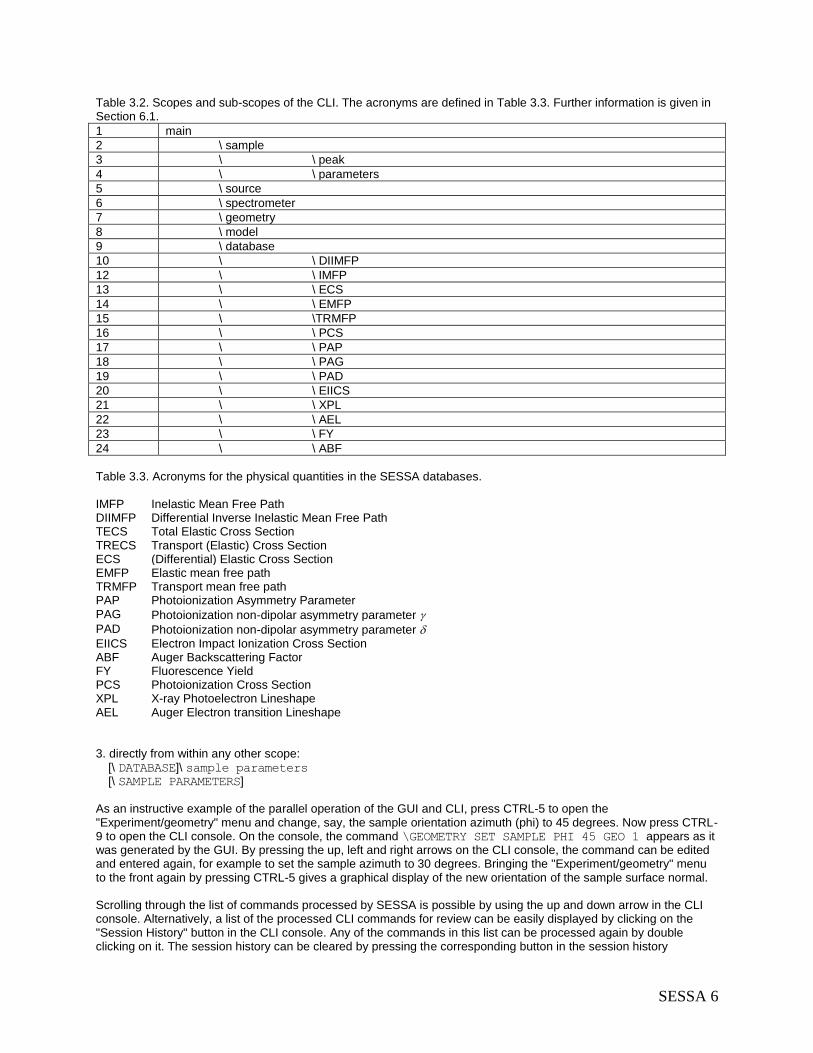
Table 3.2. Scopes and sub-scopes of the CLI. The acronyms are defined in Table 3.3. Further information is given in Section 6.1.

1 main

2 \ sample

3 \ \ peak

4 \ \ parameters

5 \ source

6 \ spectrometer

7 \ geometry

8 \ model

9 \ database

10 \ \ DIIMFP

12 \ \ IMFP

13 \ \ ECS

14 \ \ EMFP

15 \ \TRMFP

16 \ \ PCS

17 \ \ PAP

18 \ \ PAG

19 \ \ PAD

20 \ \ EIICS

21 \ \ XPL

22 \ \ AEL

23 \ \ FY

24 \ \ ABF

Table 3.3. Acronyms for the physical quantities in the SESSA databases. IMFP Inelastic Mean Free Path DIIMFP Differential Inverse Inelastic Mean Free Path TECS Total Elastic Cross Section TRECS Transport (Elastic) Cross Section ECS (Differential) Elastic Cross Section EMFP TRMFP

Elastic mean free path Transport mean free path

PAP Photoionization Asymmetry Parameter PAG Photoionization non-dipolar asymmetry parameter PAD Photoionization non-dipolar asymmetry parameter EIICS Electron Impact Ionization Cross Section ABF Auger Backscattering Factor FY Fluorescence Yield PCS Photoionization Cross Section XPL X-ray Photoelectron Lineshape AEL Auger Electron transition Lineshape 3. directly from within any other scope: [\ DATABASE]\ sample parameters [\ SAMPLE PARAMETERS] As an instructive example of the parallel operation of the GUI and CLI, press CTRL-5 to open the "Experiment/geometry" menu and change, say, the sample orientation azimuth (phi) to 45 degrees. Now press CTRL-9 to open the CLI console. On the console, the command \GEOMETRY SET SAMPLE PHI 45 GEO 1 appears as it was generated by the GUI. By pressing the up, left and right arrows on the CLI console, the command can be edited and entered again, for example to set the sample azimuth to 30 degrees. Bringing the "Experiment/geometry" menu to the front again by pressing CTRL-5 gives a graphical display of the new orientation of the sample surface normal. Scrolling through the list of commands processed by SESSA is possible by using the up and down arrow in the CLI console. Alternatively, a list of the processed CLI commands for review can be easily displayed by clicking on the "Session History" button in the CLI console. Any of the commands in this list can be processed again by double clicking on it. The session history can be cleared by pressing the corresponding button in the session history

SESSA 7

command list. This is an important feature for producing CLI command files using the "Save session" command (see below). The great advantage of this parallel CLI/GUI interface is that a set of CLI commands can be read from or written to a text file, using the PROJECT LOAD/SAVE SESSION command or by pressing the "Load/save session" button on the CLI console. This makes it possible to process a large batch of commands. Such CLI command files can be produced in a simple way by a user without any knowledge of the CLI syntax. This can be done by a series of mouse clicks in the GUI and saving all previously entered commands by pressing the "Save session" button on the CLI console. The tutorials described in Section 7 are examples of CLI command files produced in this way. A # character at the beginning of a line in a CLI command file designates the line as a comment. Another example of a SESSA CLI file is a file by the name of "SESSA_ini.ses" that resides in the directory where the SESSA binary code is located. This file is read whenever the software starts up and the commands contained in it are processed by the CLI. This may be advantageous for a user who commonly works on problems requiring settings that differ from the default settings in SESSA. This may concern the radiation type, the instrument settings, the sample composition, and so on. A group of commands from the CLI can also be copied and pasted into word processing software and saved as a text file. Multiple files can be created in this way and loaded into SESSA to avoid the tedium and possible mistakes from using the GUI for multiple similar simulations. Similarly, a user can assemble desired setup files for a particular purpose by combining selected command lines from existing files. Finally, a user can assemble files for batch runs (e.g., for a series of XPS configurations or for a series of layer thicknesses). Each file can specify different file names to save spectra or peak intensities from a series of simulations. SESSA will create these files in the same directory as that from which setup files were loaded.

3.3 Representation of Data in SESSA A CLI command as well as an input field in the GUI may comprise special data types as indicated in Table 3.4. These data types are now described in turn. 1. integer: an integer number whose range depends on the operating system (OS) of the computer.

2. real: a real number with a range that also depends on the OS. The character e signifies exponentiation to a power

of ten. For example, the expressions 0.0099, 99.0e-4 and 99e-4 are all valid expressions for the same real number. 3. string: a string of characters. A string may contain all alphanumerical characters and special characters (%, *, etc.)

in upper or lower case. If a string contains spaces, it must be enclosed in single quotes, e.g., 'Au, 1000 eV'. 4. filename: a string of characters designating a file of the operating system with a filename valid in the operating

system. 5. DBName: a predefined string of characters designating a set of data within SESSA (see Table 3.3 and Section

4.8). 6. material: The material specifier is a special string of characters that allows the program to recognize the elements

and stoichiometry in a given material. It identifies the elements present in the sample and their chemical state, allowing the software to retrieve the relevant information. For a user, there are two different ways to enter the material in the sample menu: one way is to enter the material specifier in the format used internally by SESSA, with a special syntax (e.g., "/SI/O2/" for silicon dioxide), as explained below. The alternative method is to enter the material in a more intuitive syntax (e.g., "SiO2" for silicon dioxide). If the material is specified in this simpler more intuitive way, SESSA will translate this into the internal syntax that will be displayed in the material field in the GUI. Since the internal syntax is more powerful than the intuitive syntax, it will be described first and then the intuitive syntax. The internal material specifier consists either of a number of compound specifiers, or a number of constituent specifiers, or both. The constituent specifier, enclosed in forward slashes (/) consists of an element identifier (the usual abbreviation of the elemental name from the periodic table of the elements), a chemical state attribute (an arbitrary string specified by the user enclosed in square brackets ([ ]), and a real number describing the abundance of this species in a given layer of the compound or material: <constituent specifier> = /<element identifier>[<chemical state attribute>]<abundance>/

SESSA 8

Table 3.4: Special data types for SESSA user interaction.

1 <integer> an integer number

2 <real> a real number

3 <string> a string of characters

4 <filename> a string designating a file of the OS

5 <Dbname> a string designating a set of data within SESSA

6 <material> a material specifier

7 <subshell> a subshell specifier

Here <element identifier> represents a chemical symbol (e.g., H, He, Li, Be, ... ) (case insensitive)

<chemical state attribute> is an arbitrary string indicating the chemical state <abundance> is a positive real number indicating the relative abundance of the element in a given layer.

If the chemical state attribute is omitted, the software recognizes the constituent as the elemental form of the chemical species. If the relative abundance is omitted, it is taken to be unity. A compound specifier consists of a number of constituent specifiers enclosed in parentheses '( )' followed by the relative abundance of the considered compound, or by several compound specifiers. Nesting of compound specifiers is allowed. Again, if the abundance is omitted, it is taken to be unity. <compound specifier> = (A)xA(B)xB … where A, B, … are arbitrary combinations of compound or constituent specifiers and xA, xB are their relative atomic abundances. The concentration of compound A in this material is given by:

...

BA

AA

xx

xc . (3.1)

If the compound A is given by the constituents A1, A2, ... etc. with abundances xA1, xA2, ... etc., then A is specified as follows:

/.../// 2211 AA xAxAA (3.2)

and the concentration of the species Ai in the considered material is given by:

...) (

BA

jj

AiAi xx

xA

xc . (3.3)

The more intuitive syntax for the material specifier is a string of characters containing the chemical symbols of the elements and their abundances in the material without forward slashes. In this case the specification of the chemical symbols of the elements is case sensitive, e.g. "Si", "Fe", "Au" are valid chemical symbols for silicon, iron and gold, respectively, while "SI", "FE" and "AU" are invalid in the intuitive syntax. The reason is simply that case insensitive chemical symbols are not uniquely identifiable. For example "SI" might be interpreted as a sulfur-iodine compound or as silicon, "CO" might be interpreted as cobalt or carbon monoxide. The omission of the forward slashes and the case sensitivity is the main difference between the intuitive syntax and the internal syntax. The syntax for the chemical state attribute and the compound specifier is the same in both syntaxes. Some examples: (a) /S/I/O3.0e0/. A (very hypothetical) solid consisting of the three elements sulfur, iodine and oxygen, all of them present in elemental form in relative amounts of 1:1:3.

SESSA 9

(b) (/si[oxide]/O2/)99(/c/)1. A typical silicon dioxide layer that contains silicon bound to oxygen, oxygen and a carbon contamination. The relative amounts of the elements in the layer are 0.33:0.66:0.01. 7. subshell: a subshell may be specified by a string consisting of the principal quantum number n followed by the usual symbol for the angular momentum quantum number l (s for l = 0, p for l = 1, d for l = 2, and f for l = 3) and the usual symbol indicating the spin state (e.g., 1/2, 3/2, etc.). The subshell may be abbreviated to the unambiguous shortest form (e.g., 4f7 is equivalent to 4f7/2.

3.4 Output produced by SESSA Information concerning the experimental settings specified by the user, the retrieved data corresponding to these settings, and the outcome of a model calculation can be written to a number of files by selecting the

"Project/Save/Output" option in the GUI or by issuing the command PROJECT SAVE OUTPUT in the CLI. As a result,

a number of different files containing information in several categories are generated. For several categories, writing of the output can be (de)activated in the "Project/preferences" menu (see Section 4.3). 1. filenames ending with: sam_lay.txt The sample structure 2. filenames ending with sam_peak.txt, sam_par.txt Signal-electron generation and transport 3. filenames ending with exp.txt, prefs.txt The experimental settings and preferences settings 4. filenames ending with refs.txt, rems.txt References to works in the literature concerning the above and accompanying remarks 5. filenames ending with .spc, .pi, .adf These files are written if a model calculation was performed and they contain the corresponding results. The output

is divided into region data, corresponding to a certain energy-region setting for the spectrometer, and peak data, corresponding to a certain spectral line. The region data are written to files with names identified by the string "reg<region number>", where "<region number>" is an integer referring to the spectrometer region. The

peak data are written to files identified by a peak identifier, consisting of the chemical symbol followed by the transition specifier. This is either the subshell abbreviation in case of an XPS peak (e.g., 2p3) or the Auger transition specifier (e.g., L3M23M45). The file names ending with .spc contain the energy spectra of the various peaks and regions for all selected geometries. The file names ending with .pi contain the partial intensities for each peak and all geometries. If the number of geometries is larger than one, files ending with .adf are created that contain the partial intensities for the specified peak for all specified geometrical configurations. If ncol=0 is

selected in the model menu (see Section 4.9) and the number of specified geometries is larger than one, it is assumed that the angular distribution of the peak intensities (zero-order partial intensities) is of main interest. In

this case, the file all.adf is created that contain the peak intensities for all peaks as a function of the specified

geometrical configurations. 6. filenames ending with _g Files that can be loaded into the program GNUPLOT (see http://www.gnuplot.info) that has proven to be

convenient for further graphical post-processing of the simulation data. An alternative quick and convenient means to produce output is to use the PLOT SHOW DATA option in the main plot

window popup menu that displays the data contained in a plot in a separate read-only window (see Chapter 4.2), together with the relevant literature citation. The information in this window can be copied and pasted into another application for further processing.

4 RUNNING SESSA This chapter describes all commands utilized by the command line interface (CLI) in some detail. Since a close correspondence exists between the CLI and the graphical user interface (GUI), no detailed description of the latter is given. In most cases, it is evident which component of the GUI provides the equivalence to a certain CLI command. In the CLI, however, it is often necessary within a command to specify which peak, which geometry, which layer, etc.,

one is addressing with the issued command. This situation can lead to awkward syntax such as DO SOMETHING

http://www.gnuplot.info/

SESSA 10

LAYER 1 PEAK 2 REGION 3. In the GUI, the situation can be handled in a more elegant way within a submenu by

means of one or more graphical selection tools. For example, there is an equivalence between the "Choose peak" and "Choose layer" selection boxes in the "Sample/parameters" menu in the GUI and the peak number and layer number in the equivalent CLI command (SAMPLE PARAMETERS PLOT ECS PEAK <PEAK #> LAYER <LAYER #>).

In the following sections concerning the CLI syntax of various scopes, < > represents a parameter of the type indicated that has to be entered by the user, while [ ] is an optional parameter that may be omitted. The energies displayed in and accepted by both the GUI and the CLI can be specified either on a kinetic energy scale or, in the case of incoming photons, it may optionally be specified on a binding energy scale. The user can set a preference in the "Project/preferences" menu. Depending on this setting, an energy referred to in the remainder of this Section is implied to be specified either on a kinetic or a binding-energy scale.

4.1 The PROJECT Menu

The Project menu in the GUI is shown in Fig. 4.1. The CLI console, the separate plot window, and the preferences dialog can be opened from within the project menu. The plot window, the CLI console, and the preferences dialog are described below. The project menu is otherwise equivalent to the project menu in the CLI, as described in the next Section.

Figure 4.1. Graphical user interface for the PROJECT Menu. 4.1.1 Synopsis of CLI Commands

1. PROJECT SAVE SESSION <string> Save command history to the file <string >. Each command typed in during your session (or generated by

clicking in the GUI) is written to a text file. This file may be later executed, but it can also be edited and modified to enable processing of a batch of commands. In this way, one can generate calibration curves of various kinds, angular distributions of peak intensities, etc.

2. PROJECT SAVE OUTPUT <string> Save output to files beginning with the ID <string >. 3. PROJECT LOAD SESSION <string>

Load command history from the file <string >. 4. PROJECT RESET Clear all data and reset everything to the default values.

4.2 The PLOT Menu Data can be displayed in a separate window that allows full user access to the display parameters by double clicking the window. Various quantities in SESSA can be graphically displayed. These displays cannot in any way be changed by the user. However, by double clicking on any of these windows, a separate plot window is opened providing full user access to the plot settings, as shown in Fig. 4.2 as an example. This plot window is also accessible via the "Project/Plotwindow" command in the GUI and through appropriate commands (pertaining to the quantity on display) in the CLI. A right mouse click in the plot window activates a popup menu that opens the plot settings window (see Fig. 4.2), a comprehensive menu for manipulating the settings of the display. Alternatively, the quick axis settings menu can be activated. The latter allows a user to set the axis range, and to turn on/off an axis grid or a logarithmic scaling of the axis. Furthermore, the popup menu can be utilized to open a read-

SESSA 11

Fig. 4.2. Graphical user interface for the PLOT and the PLOT/Settings Menu. only window displaying the data contained in the plot along with the corresponding references, as indicated in Fig. 4.3. 4.2.1 Synopsis of CLI Commands

1. PLOT SET LOG X Selects the x-axis for logarithmic scaling. 2. PLOT SET LOG Y Selects the y-axis for logarithmic scaling. 3. PLOT SET NOLOG X

Selects the x-axis for linear scaling. 4. PLOT SET NOLOG Y

Selects the y-axis for linear scaling. 5. PLOT SET AUTO XRANGE

Selects the upper and lower limits of the x-axis for automatic scaling. 6. PLOT SET AUTO XLOW

Selects the lower limit of the x-axis for automatic scaling. 7. PLOT SET AUTO XHIGH

Selects the upper limit of the x-axis for automatic scaling. 8. PLOT SET AUTO YRANGE

Selects the upper and lower limits of the y-axis for automatic scaling. 9. PLOT SET AUTO YLOW

Selects the lower limit of the y-axis for automatic scaling.

SESSA 12

Figure 4.3. Read-only window displaying the data contained in the Plot window. The data in this window can be transferred to other software by means of copy and paste operations for further processing. 10. PLOT SET AUTO YHIGH

Selects the upper limit of the y-axis for automatic scaling. 11. PLOT SET GRID X

Selects the x-axis grid for drawing. 12. PLOT SET GRID Y

Selects the y-axis grid for drawing. 13. PLOT SET NOGRID X

Disable drawing of the grid for the x-axis.

SESSA 13

14. PLOT SET NOGRID Y

Disable drawing of the grid for the y-axis. 15. PLOT SET LEGEND

Activate drawing of a legend in the plot. 16. PLOT SET NOLEGEND

Deactivate drawing of a legend in the plot.

17. PLOT SET XRANGE <string> Sets the x-axis range to <string >. Syntax to specify the range: xlow:xhigh. Example: set xrange 1400:1500.

18. PLOT SET YRANGE <string> Sets the y-axis range to <string >. Syntax to specify the range: ylow:yhigh. Example: set yrange 1400:1500.

19. PLOT SET CURVETITLE <string> [CURVE <int>]

Sets the legend of the curve to <string >, where CURVE is the number of the selected curve. 20. PLOT SET LTYPE <int> [CURVE <int>]

Sets the linetype of the selected curve (0- data points; 1- solid line; 2- data points and line), where CURVE is the number of the selected curve.

21. PLOT SET COLOR <int> [CURVE <int>]

Sets the color of the selected curve (integer between 0 and 35), where CURVE is the number of the selected curve.

22. PLOT SET WIDTH <int> [CURVE <int>]

Sets the linewidth of the selected curve (integer between 0 and 3), where CURVE is the number of the selected curve.

23. PLOT SET DASH <int> [CURVE <int>]

Sets the dash style of the selected curve (integer between 0 and 3), CURVE is the number of the selected curve. 24. PLOT SET SYMBOL <int> [CURVE <int>]

Sets the symbol style of the selected curve (integer between 1 and 10), where CURVE is the number of the selected curve.

25. PLOT SET VISIBLE CURVE <int>

Number of the selected curve. 26. PLOT SET VISIBLE ALL

Sets all curves to visible. 27. PLOT SET INVISIBLE CURVE <int>

Number of the selected curve. 28. PLOT SET INVISIBLE ALL

Selects all curves for hiding. 29. PLOT SET TITLE <string>

Sets the title of the plot to <string >. 30. PLOT SET XLABEL <string>

Sets the x-axis label of the plot to <string >. 31. PLOT SET YLABEL <string>

Sets the y-axis label of the plot to <string >. 32. PLOT SAVE DATA <string>

Save plot data of each curve to the text file <string >. 33. PLOT SAVE PDF <String> [ PAGESIZE <String> ]: Save plot as pdf to the file <string>.

SESSA 14

34. PLOT SAVE PNG <String> [ WIDTH <Integer> HEIGHT <Integer> ]: Save plot as png to the file <string>. 35. PLOT SAVE BMP <String> [ WIDTH <Integer> HEIGHT <Integer> ]: Save plot as bmp to the file <string>. 36. PLOT SAVE JPG <String> [ WIDTH <Integer> HEIGHT <Integer> ]: Save plot as JPG to the file <string>. 37. PLOT SAVE SVG <String>: Save plot as svg to the file <string>.

4.3 The PREFERENCES Menu The preferences menu allows a user to control various parameters determining the operation of SESSA as shown in Fig. 4.4.

Figure 4.4. Graphical user interface for the PREFERENCES Menu. 4.3.1 Synopsis of CLI Commands

1. PREFERENCES SET NDIIMFP <int>

Set the number of different distributions of energy losses for the upper two layers in the sample. When the default value is chosen (NDIIMFP=1), it is assumed in a simulation that the differential inelastic mean free path is the same for all depths. This assumption usually provides a satisfactory approximation. However, if the electronic structures of the first two layers of the sample are substantially different, this difference may be observed in the loss features on the low-kinetic-energy side of the main peaks. In such cases it may be advisable to choose (NDIIMFP=2). Note that this may considerably increase the computation time for a simulation. Choosing yet another distribution of energy losses for deeper layers is not possible, but such effects will hardly ever be observable in an experimental spectrum.

SESSA 15

2. PREFERENCES SET THRESHOLD <double> (for Threshold)

Sets a threshold determining whether a peak retrieved from a database should actually be taken into account in any of the energy regions, as defined in the spectrometer menu. If the fractional area of a peak within the region is below this threshold, the peak is rejected from the peak list. The default value is 0.9.

3. PREFERENCES SET AES_THRESHOLD <double> (for Auger-peak threshold) Sets a threshold determining whether an Auger peak retrieved from a database should actually be taken into

account in any of the energy regions, as defined in the spectrometer menu. If the intensity of an Auger peak (estimated from the multiplicities of the subshells involved in the Auger transition) is less than this threshold times the maximum intensity for other Auger peaks from the same element within the same energy region, the peak is rejected from the peak list. The default value is 0.05.

4. PREFERENCES SET PLOT_ZERO <double>

Sets the smallest positive number displayable in a logarithmic plot. 5. PREFERENCES SET ENERGY_SCALE KINETIC

Sets the energy scale to kinetic energy. 6. PREFERENCES SET ENERGY_SCALE BINDING

Sets the energy scale to binding energy if the excitation is with photons. 7. PREFERENCES SET OUTPUT SAMPLE <string>

If <string> = true, information concerning the sample composition is included in the output. 8. PREFERENCES SET OUTPUT PARAMETERS <string>

If <string> = true, information concerning the parameters for electron generation and transport is included in the output.

9. PREFERENCES SET OUTPUT EXPERIMENT <string>

If <string> = true, information concerning the experimental settings is included in the output.

10. PREFERENCES SET DENSITY_SCALE MASS Sets the density units to mass density. 11. PREFERENCES SET DENSITY_SCALE ATOMIC Sets to density units to atomic density 12. PREFERENCES SHOW

Show the values of the parameters in the PREFERENCES menu (only available in the CLI).

4.4 The SAMPLE Menu This menu controls the parameters specifying the structure of the sample and the physical parameters of the sample of relevance for the particular experimental conditions, as indicated in Fig. 4.5. The sample is conceived to consist of a number of non-crystalline and continuous layers each with a given composition, density and thickness. The interface between the various layers is assumed to be ideally flat, except for the vacuum-solid interface that may exhibit a certain morphology. Presently, five different types of nanostructured surfaces can be modeled by the SESSA software: 1. Flat planar layered surfaces, as shown in Fig. 4.5(a) 2. Rough layered surfaces, as shown in Fig. 4.5(b) 3. Islands (consisting of a single material) on top of a flat layered surface, as shown in Fig. 4.5(c) 4. Spheres (consisting of a single material) on top of a flat layered surface, as shown in Fig. 4.5(d) 5. Layered spheres on top of a flat layered surface (consisting of a single material), as shown in Fig. 4.5(e)

SESSA 16

Figure 4.5(a). Graphical user interface for the SAMPLE Menu when the selected morphology is a planar sample. The white numbers in red circles designate layer numbers.

. Figure 4.5(b). Graphical user interface for the SAMPLE Menu when the selected morphology is a surface with a specified roughness. The white numbers in red circles designate layer numbers.

SESSA 17

Figure 4.5(c). Graphical user interface for the SAMPLE Menu for morphology type “islands”. The white numbers in red circles designate layer numbers.

Figure 4.5(d). Graphical user interface for the SAMPLE Menu for morphology type “spheres”. The white numbers in red circles designate layer numbers.

SESSA 18

Figure 4.5(e). Graphical user interface for the SAMPLE Menu for morphology type “layered spheres”. The white numbers in red circles designate layer numbers.

A desired sample morphology is selected from the morphology box in the top-right corner of each Sample screen (with the Layer tab) shown in Fig. 4.5. The user can then set parameters for the chosen nanomorphology, as shown in the relevant screens of Fig. 4.5. Commands for the control of individual morphology parameters are explained in detail in Section 4.4.4. The designation of layer numbers is indicated in Fig. 4.5 as white numbers in red circles. The material in a given layer is specified by a special string describing the elemental composition (see below). All relevant parameters for a specified material are retrieved by the expert system and can be inspected and changed in the "Sample peak" menu (see Section 4.4.5) and the "Sample parameter" menu (see Section 4.4.3). A value for the density of each layer is also determined for each layer. For elemental solids, this quantity is read from a database; for most other materials, it is estimated on the basis of elemental densities of the constituents in each layer. The estimated density may be in error by more than 100 %. It is therefore recommended that the user should specify a more realistic value for the density in such cases. 4.4.1 The SAMPLE LAYER Menu

This menu (selected by the Layer tab in the Sample menus of Fig. 4.5) controls the parameters specifying the thickness, density, bandgap energy, number of valence electrons per atom or molecule, number of atoms per molecule, composition, thickness, and roughness of the surface. SESSA will automatically enter appropriate values (based on the chosen composition of the layer) for the number of valence electrons per atom or molecule and for number of atoms per molecule. SESSA has a library of densities for elemental solids but only provides rough estimates for compounds, and the user should check these estimates. The default setting for density units is number of atoms per cubic centimeter but this can be changed to mass density (expressed in g/cm

3) using the Preferences menu (see Section 4.3). The bandgap energy Eg is needed for estimating

IMFPs from the TPP-2M formula [6], and values for many compounds can be found in a number of sources [75-80]. If a value for the bandgap energy Eg cannot be found for the compound of interest, it is satisfactory to estimate this parameter because the IMFP is not a sensitive function of Eg [81,82]. For highly ionic compounds such as the alkali halides, Eg is generally between 6 eV and 11 eV. For oxides, Eg values are often between 1 eV and 9 eV.

SESSA 19

4.4.2 Synopsis of CLI Commands

1. SAMPLE ADD LAYER <string> THICKNESS <double> [ABOVE <int>]

Adds a new layer above the selected layer. The material of the layer is specified by the material identifier <string > (see Section 3.3).

THICKNESS: Specify the thickness (in Å) of the layer to be added.

ABOVE: Add the layer above the specified layer instead of above the layer that is selected in the "Choose layer" box.

2. SAMPLE DELETE LAYER <int>

Delete the specified layer. 3. SAMPLE RESET

Reset the complete sample structure to its default (a homogeneous Si sample). 4. SAMPLE SET ACTLAY <int>

Set the number of a given layer to which all following commands apply per default. 5. SAMPLE SET DENSITY <double> [LAYER <int>]

Set the density of a given layer (in atoms/cm3), where LAYER is the number of the selected layer.

6. SAMPLE SET EGAP <double> [LAYER <int>]

Set the band-gap energy (in eV) of a material in a given layer, where LAYER is the number of the selected layer.

7. SAMPLE SET NVALENCE <int> [LAYER <int>]

Set the number of valence electrons per atom or molecule of a material in a given layer, where LAYER is the number of the selected layer.

8. SAMPLE SET NATOMS <int> [LAYER <int>]

Set the number of atoms per molecule of a material in a given layer, where LAYER is the number of the selected layer.

9. SAMPLE SET MATERIAL <string> [LAYER <int>]

Set the material of a given layer by providing a material specifier <string > (see Section 3.3), where LAYER is the number of the selected layer.

10. SAMPLE SET THICKNESS <double> [LAYER <int>]

Set the thickness (in Å) of a given layer, where LAYER is the number of the selected layer. 11. SAMPLE SHOW SAMPLE

Show the parameters describing the sample structure in the CLI. 12. SAMPLE SHOW LAYER <int>

Show the parameters describing a single layer in the sample in the CLI. 13. SAMPLE PLOT SAMPLE

Graphical display of the concentration-depth profile of the sample. 4.4.3 The SAMPLE MORPHOLOGY Menu

This menu (selected in the box at the top right corner of the Sample graphical user interfaces shown in Figs. 4.5(a) to 4.5(e) allows the user to select a particular nanomorphology for the sample surface. Islands, spheres, and layered spheres are assumed to lie in a periodic array on the surface; the user can, however, can vary the periodicity in both the x and the y directions. 4.4.4 Synopsis of CLI Commands

1. SAMPLE MORPHOLOGY SHOW Displays information about the morphology of the sample as specified by the user.

SESSA 20

2. SAMPLE MORPHOLOGY SET PLANAR Morphology of the surface is a planar surface with a number of parallel layers consisting of different materials.

3. SAMPLE MORPHOLOGY SET ROUGHNESS Morphology of the surface is a rough surface.

4. SAMPLE MORPHOLOGY SET ISLANDS Morphology of the surface is a planar surface with an optional number of parallel layers and with pyramid-shaped islands consisting of a single material on top.

5. SAMPLE MORPHOLOGY SET SPHERES Morphology of the surface is planar surface with an optional number of parallel layers and with spheres consisting of a single material on top.

6. SAMPLE MORPHOLOGY SET LAYERED_SPHERES Morphology of the surface is a planar surface with an optional number of parallel layers and with layered spheres on top.

7. SAMPLE MORPHOLOGY SET RSA <double>

Set the roughness of the sample surface. A rough surface is assumed to consist of tilted surface segments with a certain distribution of tilt angles. The roughness is specified by the relative surface area (RSA), that is the mean value of the reciprocal of the cosine of the tilt angles. In other words, the relative surface area is the area of the surface when measured along the tilted surface segments, divided by the area of the surface segments projected onto the global surface. Consequently, RSA=1 represents an ideally smooth surface. Realistically rough surfaces are described by an RSA value between 1.05 and 1.2.

8. SAMPLE MORPHOLOGY SET X_LENGTH <double> Set the length of the islands along the x-axis (in Angstroms).

9. SAMPLE MORPHOLOGY SET Y_LENGTH <double> Set the length of the islands along the y-axis (in Angstroms). 10. SAMPLE MORPHOLOGY SET X_PERIOD <double>

Set the repetition period of the selected nanostructure along the x-axis (in Angstroms).

11. SAMPLE MORPHOLOGY SET Y_PERIOD <double> Set the repetition period of the selected nanostructure along the y-axis (in Angstroms).

12. SAMPLE MORPHOLOGY SET X_INCLINATION <double> For islands, set the inclination angle of each side plane with respect to the perpendicular to the x-axis (in degrees).

13. SAMPLE MORPHOLOGY SET Y_INCLINATION <double> For islands, set the inclination angle of each side plane with respect to the perpendicular to the y-axis (in degrees).

14. SAMPLE MORPHOLOGY SET HEIGHT <double> Set the height of the islands (in Angstroms).

15. SAMPLE MORPHOLOGY SET Z_HEIGHT <double> Set the height of the centre of the sphere above the planar surface (in Angstroms). This value should be less than or equal to half the radius of the spheres.

16. SAMPLE MORPHOLOGY SET RADIUS <double> Set the radius of the nanospheres (in Angstroms).

4.4.5 The SAMPLE PARAMETERS Menu

This menu (selected by the Parameters tab in the Sample menu of Fig. 4.5) controls the parameters for the electron/solid interaction as shown in Fig. 4.6.

SESSA 21

Figure 4.6. Graphical user interface for the SAMPLE PARAMETERS Menu.

SESSA 22


1. SAMPLE PARAMETERS SET IMFP VALUE <double> PEAK <int> LAYER <int>

Set the value of the inelastic mean free path (IMFP) for a given peak in a given layer (in Å).

PEAK: Number of the selected peak.

LAYER: Number of the selected layer. 2. SAMPLE PARAMETERS SET IMFP DATABASE <string> LAYER <int>

Select a database for retrieval of IMFP values, where LAYER is the number of the selected layer. 3. SAMPLE PARAMETERS SET IMFP MATERIAL <string> LAYER <int>

Option to search the database of IMFP values derived from optical data. In this case, the material identifier should be a string as described in Section 3.3 (e.g., Si, SiO2, TiC, etc.). Note that optical data are only available for a limited number of materials. If the requested material is not found, the default database for the IMFP is automatically invoked. This default returns an estimate for the IMFP derived from the TPP-2M formula [6] (see also "help database imfp show" for a list of available databases for this quantity). LAYER is the number of the selected layer.

4. SAMPLE PARAMETERS SET EMFP VALUE <double> PEAK<int>LAYER <int>

Set the value of the elastic mean free path (EMFP) (in Å) for a given peak in a given layer.


LAYER: Number of the selected layer. 5. SAMPLE PARAMETERS SET EMFP DATABASE <string> LAYER <int>

Select a database to retrieve the value of the EMFP (see also "help database emfp show" for a list of available databases for this quantity), where LAYER is the number of the selected layer.

6. SAMPLE PARAMETERS SET TRMFP VALUE <double> PEAK <int> LAYER <int>

Set the value of the transport mean free path (TRMFP) (in Å) for a given peak in a given layer.


LAYER: Number of the selected layer. 7. SAMPLE PARAMETERS SET TRMFP DATABASE <string> LAYER <int>

Select a database to retrieve the value of the TRMFP (see also "help database trmfp show" for a list of available databases for this quantity), where LAYER is the number of the selected layer.

8. SAMPLE PARAMETERS SET ECS DBNAME <string>PEAK <int> [LAYER<int>]

Select a database to retrieve the value of the elastic cross section (ECS) (see also "help database ecs show" for a list of available databases for this quantity).

DB NAME: Name of the database.


LAYER: Number of the selected layer. 9. SAMPLE PARAMETERS SET DIIMFP DATABASE <string> LAYER <int>

Select a database to retrieve the value of the differential inverse inelastic mean free path (DIIMFP) (see also "help database diimfp show" for a list of available databases for this quantity), where LAYER is the number of the selected layer.

10. SAMPLE PARAMETERS SET DIIMFP MATERIAL <string> LAYER <int>

Option requesting the program to search the database of optical data for evaluation of the DIIMFP. In this case the material identifier should be an ordinary (non-case sensitive) string (e.g., Si, Sio2, TiC, etc.). Note that optical data are only available for a limited number of materials. If the requested material is not found, the default database for the DIIMFP is automatically invoked. This default returns Tougaard's universal DIIMFP [7]. LAYER is the number of the selected layer.

11. SAMPLE PARAMETERS SHOW PEAK <int>

Show information about the electron-solid interaction for the selected peak in the CLI.

SESSA 23

12. SAMPLE PARAMETERS PLOT ECS PEAK <int> [LAYER <int>] Display the elastic cross section for given peak and layer. Note that for a layer containing a compound, the elastic cross section is a weighted average of the elemental cross sections for the elements comprising the compound.


LAYER: Number of the selected layer. 13. SAMPLE PARAMETERS PLOT DIIMFP [LAYER <int>] [PEAK <int>]

Display the differential inverse inelastic mean free path for a given layer.

LAYER: Number of the selected layer.

PEAK: Number of the selected peak. 4.4.7 The SAMPLE PEAK Menu

This menu (selected by the Peaks tab in the Sample menu of Fig. 4.5) controls the attributes of the peaks in the sample that contribute to the specified energy regions, as shown in Fig. 4.7. The peaks of signal electrons that have a source energy distribution lying within the energy regions of the spectrometer, as specified by the user, can be inspected and modified in this menu. Note that depending on the source energy and material of interest, it may happen that no peaks occur in the specified regions. In such cases, various data sets in SESSA are void that would otherwise contain information on the signal-electron peaks and parameters associated with them. A peak for an element may contain a number of subpeaks that are described by a functional form, relative height and width, or are given by an empirical peak shape read from a data file. Presently, SESSA does not contain detailed information on intrinsic peak shapes: the intrinsic peak is assumed to be described sufficiently well in terms of a Gaussian, Lorentzian or Doniach-Sunjic peak shape. With each peak, there are associated a number of parameters such as the subshell identifier, cross section, fluorescence yield (only for Auger transitions), etc. The graphical display for the sample peak menu shows the intrinsic peak shape by default. By means of the "Choose data" box, a user can choose to change the display to the simulated spectrum or the simulated partial intensities. By double-clicking on the display, a new window opens with a display that can be modified by the user. A right mouse click in the new window gives options for showing and saving the displayed data. The angular distribution of photoelectrons emitted from an atom is calculated in SESSA using the formula given by Cooper [71]:

cossin)cos()1cos3(

21

4

22nl

d

d (4.1)

where nl is the total photoionization cross section, is the dipole asymmetry parameter, and are the non-dipole

asymmetry parameters, is the angle between the direction of photoelectron emission and the polarization

direction, and is the angle between the direction of photoelectron emission and the plane defined by the X-ray and

polarization directions. The non-dipolar terms in Eq. (4.1) generally have a negligible effect on the angular distribution

of emitted photoelectrons for typical laboratory X-ray sources with Al and Mg anodes (i.e., for Al K and Mg K X-rays). However, these terms can significantly affect the angular distributions for higher photon energies, such as for

Ag L X-ray sources or when using synchrotron radiation with energies higher than a few keV. We note here that there is only one database in SESSA for the three photoelectron asymmetry parameters (i.e., the

parameters , , and in Eq. (4.1)). This is the database PAP3 (described in Section 6.1.8(c)) with the parameter values computed by Trzhaskovskaya, Nefedov, and Yarzhemsky [38, 39]. If a different database is selected for the

dipolar parameter , values of the non-dipolar parameters and will not be retrieved from this source. We note that Trzhaskovskaya et al. calculated photoionization cross sections and photoionization asymmetry parameters only for photon energies up to 5 keV above each photoionization threshold. Linear extrapolations were made to these values so that cross sections and asymmetry parameters would be available in SESSA for larger photon energies. These extrapolations could introduce uncertainties of more than 30% in the values of the derived parameters. To enable a more realistic simulation of peak shapes in SESSA, a chemical shift may be specified which will appropriately modify the energy of a peak (which can be a specified peak or a chemical component of a peak as indicated by the chemical state attribute). While the parameters of the sample peak menu can be manipulated in the GUI in the usual way, an additional feature was implemented in Version 1.2 of SESSA for the chemical shift. An appropriate value for the chemical shift may be entered by the user or the chemical shift database may be browsed

SESSA 24

Figure 4.7. Graphical user interface for the SAMPLE PEAK Menu. by clicking the "browse database" button. A menu for selecting the chemical shift will pop up, as illustrated in Fig. 4.8. Here all entries from Version 4.0 of the NIST XPS Database (http://srdata.nist.gov/xps) for chemical shifts are displayed for the selected peak, together with some information about the chemical state and the source from which this information was taken. The listings in each column can be sorted alphabetically or numerically by clicking on the column heading. By double clicking on the most appropriate value, or by clicking the button "select chemical shift," the corresponding value is entered into the peak settings pane of the sample peak menu. The chemical shift database from the NIST XPS Database includes chemical shifts for the material that were measured on a single instrument and a larger number of calculated chemical shifts. The latter shifts were calculated as difference of the binding energy for the line and compound that was reported in the particular data source and a reference binding energy for the same line of the elemental solid.

http://srdata.nist.gov/xps

SESSA 25

Fig. 4.8. Graphical user interface for browsing the chemical shift database. In the GUI, convenient peak list management tools are available as illustrated in Figs. 4.7 and 4.9. The main function of the peak list management tools is to facilitate deletion of a large number of peaks simultaneously in order to increase the simulation speed and to make it easier for a user to focus on a few selected peaks of special interest for the considered application. Selecting a peak for deletion is achieved by clicking the box to the left of a peak in the peak list. By means of a right mouse click anywhere in the peak list pane, it is possible to select all peaks, to select all Auger peaks, all XPS peaks, or to uncheck all peaks (see Fig. 4.9). By clicking the “Delete checked peak(s)” button in the sample peak menu, the selected peaks can be deleted. To restore the peak list to the default set corresponding to the peaks retrieved by the expert system, the material of the corresponding layer needs to be entered again in the sample layer menu, e.g., by selecting the material in the material field and pressing enter. Individual peaks can be entered manually, if desired, by using the "add peak" button in the sample peak menu. Note that the peak for which the peak settings are displayed in the sample peak menu is indicated by a blue background in the peak list, while the checkboxes on the left of each peak merely indicate whether it has been marked for deletion. Three types of data can be selected for graphical display in the SAMPLE PEAK menu by appropriate choice in the pull-down menu within the display peak window (top right region in Fig. 4.7). For each peak selected in the top left of Fig. 4.7, the user can choose one of the following displays: (1) the peak shape (default); (2) the peak spectrum; and (3) partial intensities. The peak shape represents the shape of the peak (i.e., the normalized energy distribution of the photoelectrons or Auger electrons emitted by the source atom) set by the user in the "peak settings" and "subpeak settings" menus shown in Fig. 4.7. The peak spectrum displays the simulated photoelectron or Auger-electron peak, i.e., the energy distribution of the photoelectrons or Auger electrons as emitted from the sample surface and as seen by the analyzer. This spectrum includes energy losses as a result of single or multiple inelastic scattering (often referred to as the "inelastic tail"). The partial intensities represent the number of signal electrons that reach the detector (again for the given spatial distribution of signal-electron sources from a simulation) after participating in a given number of inelastic collisions.

SESSA 26

Fig. 4.9. Portion of the graphical user interface for the SAMPLE PEAK Menu (Fig. 4.7) after a right mouse click in the peak list pane. 4.4.8 Synopsis of CLI Commands

1. SAMPLE PEAK SET ACTPEAK <int>

Set the peaks in the sample to which all of the following commands apply by default. 2. SAMPLE PEAK SET CHEMSHIFT VALUE <Double> [ PEAK <int> ] Set the value of the chemical shift in eV for a given peak. 3. SAMPLE PEAK SET CHEMSHIFT DBENTRY <Integer> [ PEAK <int> ] Select an entry from the chemical shift database. 4. SAMPLE PEAK SET ABF VALUE <double> [PEAK <int>]

Set the value of the Auger backscattering factor (ABF) for a given peak, where PEAK is the number of the selected peak.

5. SAMPLE PEAK SET ABF DATABASE <string> [PEAK <int>]

Select a database to retrieve the value of the ABF (see also "help database ABF show" for a list of available databases for this quantity), where PEAK is the number of the selected peak.

SESSA 27

6. SAMPLE PEAK SET FY VALUE <double> [PEAK <int] Set the value of the fluorescence yield (FY) for a given peak, where PEAK is the number of the selected peak.

7. SAMPLE PEAK SET FY DATABASE <string> [PEAK <int>]

Select a database to retrieve the value of the FY (see also "help database FY show" for a list of available databases for this quantity), where PEAK is the number of the selected peak.

8. SAMPLE PEAK SET ANISOTROPY <double> PEAK <integer> [DBNAME <string>] BETA DELTA GAMMA

Set the asymmetry parameters (PAP) for the photoionization cross section of a given peak in XPS. By default, the dipolar asymmetry parameter will be set. Use of the optional key words DELTA and GAMMA will change the non-dipolar parameters accordingly. Alternatively, this command can be used to set the database for retrieval of these quantities for a given peak.

DBNAME: If the DBNAME option is specified, the photoionization asymmetry parameters are retrieved from the database indicated. See also "help database PAP show" for a list of available databases for this quantity.


BETA: Set the dipolar asymmetry parameter (default choice).

DELTA: Set the non-dipolar asymmetry parameter .

GAMMA: Set the non-dipolar asymmetry parameter . 9. SAMPLE PEAK SET CROSS_SECTION <double> [DBNAME <string>] PEAK <int>

Set the ionization cross section (in Å2) associated with the peak for the specified incoming radiation. When

electrons are used as exciting radiation, the cross section is the electron-impact ionization cross section (EIICS). When photons are used, the cross section is the photoionization cross section (PCS).

DBNAME: Tells the software to retrieve the relevant cross section from the specified database (see also "help database EIICS show" for a list of available databases for this quantity).

PEAK: Number of the selected peak. 10. SAMPLE PEAK SET TYPE <string> [PEAK <int>] SUBPEAK <int>

Set the subpeak type. The possible subpeak types are: GAUSS, LORENTZ, DONIACH_SUNJIC, EMPIRICAL (see Section 4.4.5). Any peak in the spectrum may be described by a linear combination of several subpeaks, each with a position, width, and relative intensity.


SUBPEAK: Number of the selected subpeak. 11. SAMPLE PEAK SET WIDTH <double> [PEAK <int>] SUBPEAK <int>

Set the width of the subpeak (in eV) (ignored for peaks described by empirical data). The width of the value of

the parameter describing the peak width for the selected subpeak type (e.g., the Gaussian width is the value of in the Gaussian expression).


SUBPEAK: Number of the selected subpeak. 12. SAMPLE PEAK SET POSITION <double> [PEAK <int>] SUBPEAK <int>

Set the energy (in eV) of the subpeak position (ignored for peaks described by empirical data).


SUBPEAK: Number of the selected subpeak. 13. SAMPLE PEAK SET HEIGHT <double> [PEAK <int>] SUBPEAK <int>

Set the relative height of the subpeak (in arbitrary units).


SUBPEAK: Number of the selected subpeak. 14. SAMPLE PEAK SET ASYMMETRY <double> [PEAK <int>] SUBPEAK <int>

Set the asymmetry parameter for the Doniach-Sunjic formula (ignored for other peak types).


SUBPEAK: Number of the selected subpeak. 15. SAMPLE PEAK SET CHEMSTATID <string> [PEAK <int>]

Set the chemical state identifier of the peak. The chemical state identifier is an arbitrary string of characters that may be provided by a user to distinguish between the same atoms present in different states in the sample. It is

SESSA 28

not in any way interpreted by SESSA, but merely used to label peaks of the same element present in a different form (e.g., a different physical or, more commonly, chemical state) in the specimen. In a simulation, all peaks of an element corresponding to the same transition but with a different chemical state identifier are treated as separate peaks. PEAK is the number of the selected peak.

16. SAMPLE PEAK SET SENSFAC <double> [PEAK <int>]

Set the sensitivity factor of the peak. This quantity is a correction factor for Auger peaks in cases for which the fluorescence yield and Coster-Kronig transition probability are not well known, where PEAK is the number of the selected peak.

17. SAMPLE PEAK ADD AESPEAK ENERGY <double> TRANSITION <string> SUBSHELLID <string> ELEMENT

<string> [CHEMSTATID <string>] Add an Auger peak specified by the user to the list of peaks.

ENERGY: Energy (in eV) of the peak.

TRANSITION: The transition for the Auger peak.

SUBSHELLID: The subshell that is ionized initially and leads to the considered Auger transition.

ELEMENT: The element emitting the signal electrons.

CHEMSTATID: Chemical state label for a peak. 18. SAMPLE PEAK ADD XPSPEAK ENERGY <double> SUBSHELLID <string> ELEMENT <string> [CHEMSTATID <string>]

Add a photoelectron peak specified by the user to the list of peaks.

ENERGY: Energy (in eV) of the peak.

SUBSHELLID: Subshell of the photoelectron peak.

ELEMENT: Element emitting the signal electrons.

CHEMSTATID: Chemical state for the peak. 19. SAMPLE PEAK ADD SUBPEAK PEAK <int> ENERGY <double>

Add a subpeak to the peak data structure.


ENERGY: Specify the energy (in eV) for the subpeak. 20. SAMPLE PEAK DELETE PEAK <int> [SUBPEAK <int>]

Delete an attribute of the peak data structure.


SUBPEAK: Number of the selected subpeak. 21. SAMPLE PEAK SHOW [PEAK <int>] [SUBPEAK <int>]

Show information on the data for the peak.


SUBPEAK: Number of the selected subpeak. 22. SAMPLE PEAK LIST [PEAK <int>]

Show peak position, width parameter, relative intensity, and peak type for all peaks or for a selected peak and any of its subpeaks. PEAK is the number of the selected peak.

23. SAMPLE PEAK PLOT SPEC [PEAK <int>]

Graphical display of the partial spectrum emitted from the surface, where PEAK is the number of the selected peak.

24. SAMPLE PEAK PLOT PART_INT [PEAK <int>]

Graphical display of the partial intensities of electrons emitted from the surface, where PEAK is the number of the selected peak.

25. SAMPLE PEAK PLOT SHAPE [PEAK <int>] [SUBPEAK <int ]

Graphical display of the partial spectrum emitted at the location in the sample where the signal-electron excitation takes place.


SUBPEAK: Number of the selected subpeak.

SESSA 29

26. SAMPLE PEAK OUTPUT SPEC FILE <string> [PEAK <int>] Writes the spectrum for the selected peak to a file.

FILE: Name of the output file.

PEAK: Number of the selected peak. 27. SAMPLE PEAK OUTPUT PART_INT FILE <string> [PEAK <int>]

Writes the partial intensities for the selected peak to a file.

FILE: Name of the output file.

PEAK: Number of the selected peak. 28. SAMPLE PEAK LOAD DATA <string> [PEAK <int>] SUBPEAK <int>

Loads an ASCII file containing the peak shape of a given subpeak for an EXISTING peak. Before peak shape data can be loaded for a new peak, this peak has to be defined by adding it (see SAMPLE ADD PEAK). The expected format for each line of this file is: "energy (eV)/ one or more spaces/ intensity (arb. units)".


SUBPEAK: Number of the selected subpeak.

4.5 The SOURCE Menu This menu specifies the source of exciting radiation for an experiment, as shown in Fig. 4.10. If an attribute of the source is changed, the expert system must start a new query for many relevant quantities. This means that previous user input for any of these quantities will be lost in such cases. For example, definitions concerning the shape, position or relative intensities of a peak that was manually added by a user as well as the corresponding interaction parameters will be erased. To save such user settings, it is advisable to save the session (see the command PROJECT SAVE SESSION in Section 4.1.1). If the incoming radiation is chosen to be photons, their energy can be specified and their polarization can be specified to be circular or unpolarized by setting the linear polarization fraction to zero. If the incoming beam is partially linearly polarized, the fraction of the linearly polarized light P in the beam can be set with this command, as indicated in Fig. 4.10. It is assumed that the remaining fraction (1 - P) of the beam is circularly polarized or unpolarized. The polarization fraction only affects the angular distribution of photoelectrons in any calculation. For unpolarized or circularly polarized light, the angular distribution is rotationally symmetric around the direction of the photon momentum, while for linearly polarized light it is rotationally symmetric around the polarization vector [69,70]. The polarization direction is chosen on the GEOMETRY menu (section 4.7). If the incoming radiation is chosen to be electrons, the electron energy can be specified. 4.5.1 Synopsis of CLI Commands

1. SOURCE SET ALKA

Sets the source to Al K radiation. 2. SOURCE SET MGKA

Sets the source to Mg K radiation. 3. SOURCE SET ZRMZ

Sets the source to Zr M radiation. 4. SOURCE SET PHOTONS ENERGY <double>

Sets the source to photons with an energy as specified, where ENERGY is the photon energy (in eV). 5. SOURCE SET POLARIZATION FRACTION <double> Sets the fraction of linear polarization for the incoming light. 6. SOURCE SET ELECTRONS ENERGY <double>

Sets the source to electrons with an energy as specified, where ENERGY is the electron energy (in eV). 7. SOURCE SHOW

Shows the parameters of the SOURCE menu.

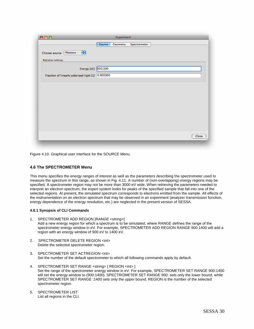
SESSA 30

Figure 4.10. Graphical user interface for the SOURCE Menu.

4.6 The SPECTROMETER Menu This menu specifies the energy ranges of interest as well as the parameters describing the spectrometer used to measure the spectrum in this range, as shown in Fig. 4.11. A number of (non-overlapping) energy regions may be specified. A spectrometer region may not be more than 3000 eV wide. When retrieving the parameters needed to interpret an electron spectrum, the expert system looks for peaks of the specified sample that fall into one of the selected regions. At present, the simulated spectrum corresponds to electrons emitted from the sample. All effects of the instrumentation on an electron spectrum that may be observed in an experiment (analyzer transmission function, energy dependence of the energy resolution, etc.) are neglected in the present version of SESSA. 4.6.1 Synopsis of CLI Commands

1. SPECTROMETER ADD REGION [RANGE <string>] Add a new energy region for which a spectrum is to be simulated, where RANGE defines the range of the

spectrometer energy window in eV. For example, SPECTROMETER ADD REGION RANGE 900:1400 will add a region with an energy window of 900 eV to 1400 eV.

2. SPECTROMETER DELETE REGION <int> Delete the selected spectrometer region. 3. SPECTROMETER SET ACTREGION <int>

Set the number of the default spectrometer to which all following commands apply by default. 4. SPECTROMETER SET RANGE <string> [ REGION <int> ]

Set the range of the spectrometer energy window in eV. For example, SPECTROMETER SET RANGE 900:1400 will set the energy window to (900:1400). SPECTROMETER SET RANGE 900: sets only the lower bound, while SPECTROMETER SET RANGE :1400 sets only the upper bound. REGION is the number of the selected spectrometer region.

5. SPECTROMETER LIST

List all regions in the CLI.

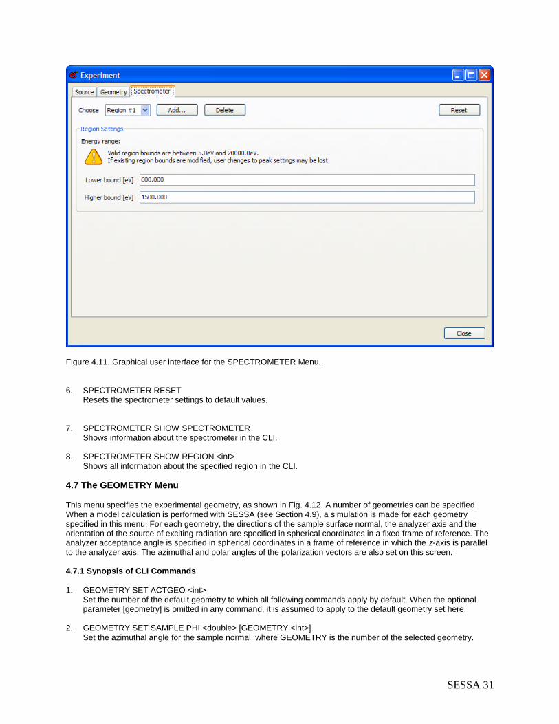
SESSA 31

Figure 4.11. Graphical user interface for the SPECTROMETER Menu. 6. SPECTROMETER RESET

Resets the spectrometer settings to default values.

7. SPECTROMETER SHOW SPECTROMETER

Shows information about the spectrometer in the CLI. 8. SPECTROMETER SHOW REGION <int>

Shows all information about the specified region in the CLI.

4.7 The GEOMETRY Menu This menu specifies the experimental geometry, as shown in Fig. 4.12. A number of geometries can be specified. When a model calculation is performed with SESSA (see Section 4.9), a simulation is made for each geometry specified in this menu. For each geometry, the directions of the sample surface normal, the analyzer axis and the orientation of the source of exciting radiation are specified in spherical coordinates in a fixed frame of reference. The analyzer acceptance angle is specified in spherical coordinates in a frame of reference in which the z-axis is parallel to the analyzer axis. The azimuthal and polar angles of the polarization vectors are also set on this screen. 4.7.1 Synopsis of CLI Commands

1. GEOMETRY SET ACTGEO <int>

Set the number of the default geometry to which all following commands apply by default. When the optional parameter [geometry] is omitted in any command, it is assumed to apply to the default geometry set here.

2. GEOMETRY SET SAMPLE PHI <double> [GEOMETRY <int>]

Set the azimuthal angle for the sample normal, where GEOMETRY is the number of the selected geometry.

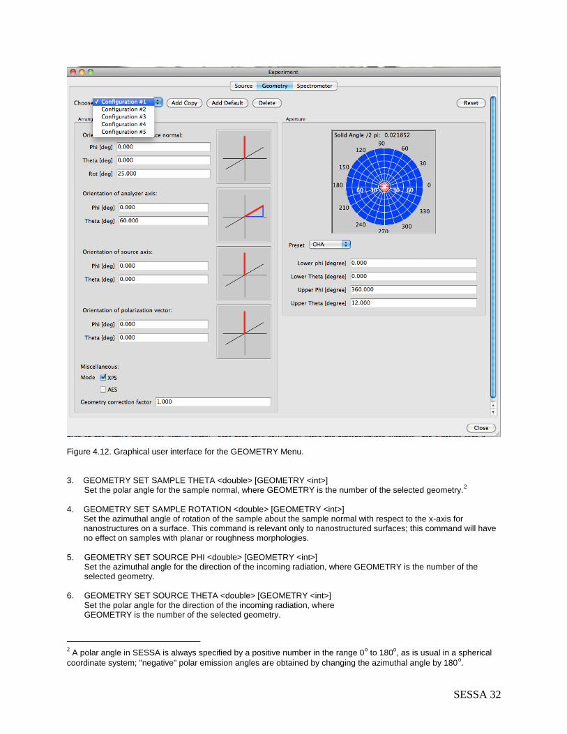
SESSA 32

Figure 4.12. Graphical user interface for the GEOMETRY Menu. 3. GEOMETRY SET SAMPLE THETA <double> [GEOMETRY <int>]

Set the polar angle for the sample normal, where GEOMETRY is the number of the selected geometry.2

4. GEOMETRY SET SAMPLE ROTATION <double> [GEOMETRY <int>]

Set the azimuthal angle of rotation of the sample about the sample normal with respect to the x-axis for nanostructures on a surface. This command is relevant only to nanostructured surfaces; this command will have no effect on samples with planar or roughness morphologies.

5. GEOMETRY SET SOURCE PHI <double> [GEOMETRY <int>] Set the azimuthal angle for the direction of the incoming radiation, where GEOMETRY is the number of the selected geometry.

6. GEOMETRY SET SOURCE THETA <double> [GEOMETRY <int>]

Set the polar angle for the direction of the incoming radiation, where GEOMETRY is the number of the selected geometry.

2 A polar angle in SESSA is always specified by a positive number in the range 0

o to 180

o, as is usual in a spherical

coordinate system; "negative" polar emission angles are obtained by changing the azimuthal angle by 180o.

SESSA 33

7. GEOMETRY SET SOURCE POLARIZATION PHI <Double> [ GEOMETRY <int> ] Set the azimuthal angle of the polarization vector. 8. GEOMETRY SET SOURCE POLARIZATION THETA <Double> [ GEOMETRY <int> ] Set the polar angle of the polarization vector. 9. GEOMETRY SET ANALYZER PHI <double> [GEOMETRY <int]

Set the azimuthal angle for the analyzer axis, where GEOMETRY is the number of the selected geometry. 10. GEOMETRY SET ANALYZER THETA <double> [GEOMETRY <int>]

Set the polar angle for the analyzer axis, where GEOMETRY is the number of the selected geometry. 11. GEOMETRY SET ANALYZER CMA [GEOMETRY <int>]

Set the analyzer aperture to that of a standard cylindrical mirror analyzer (CMA), where GEOMETRY is the number of the selected geometry.

12. GEOMETRY SET ANALYZER CHA [GEOMETRY <int>]

Set the analyzer aperture to that of a standard concentric hemispherical analyzer (CHA), where GEOMETRY is the number of the selected geometry.

13. GEOMETRY SET ANALYZER RFA [GEOMETRY <int>]

Set the analyzer aperture to that of a standard retarding field analyzer (RFA), where GEOMETRY is the number of the selected geometry.

14. GEOMETRY SET APERTURE LPHI <double> [GEOMETRY <int>]

Set the lower azimuthal angle of the analyzer aperture, where GEOMETRY is the number of the selected geometry.

15. GEOMETRY SET APERTURE UPHI <double> [GEOMETRY <int>]

Set the upper azimuthal angle of the analyzer aperture, where GEOMETRY is the number of the selected geometry.

16. GEOMETRY SET APERTURE LTHETA <double> [GEOMETRY <int>]

Set the lower polar angle of the analyzer aperture, where GEOMETRY is the number of the selected geometry. 17. GEOMETRY SET APERTURE UTHETA <double> [GEOMETRY <int>]

Set the upper polar angle of the analyzer aperture, where GEOMETRY is the number of the selected geometry. 18. GEOMETRY SET MODE XPS [GEOMETRY <int>]

Set the geometry mode to XPS. In this mode, the surface area seen by the analyzer changes as the inverse cosine of the polar emission angle with respect to the surface normal. GEOMETRY is the number of the selected geometry.

19. GEOMETRY SET MODE AES [GEOMETRY <int>]

Set the geometry mode to AES. In this mode, the surface area seen by the analyzer is independent of the emission angle. GEOMETRY is the number of the selected geometry.

20. GEOMETRY SET FACTOR <double> [GEOMETRY <int>]

Set a geometric correction factor for each geometry. Geometrical artifacts are often difficult to avoid in a real experiment, but are usually reproducible for a given instrument. Therefore, a geometry-dependent correction factor can be defined here if desired, as described in Section 5.2.3. GEOMETRY is the number of the selected geometry.

21. GEOMETRY ADD GEOMETRY [COPY <int>]

Add a geometry to the list for angle-resolved experiments, where COPY adds a geometry to the list and copies the parameter values for the previous geometry into the new geometry.

22. GEOMETRY DELETE GEOMETRY <int>

Delete the selected geometry from the list. 23. GEOMETRY LIST

List all different geometries.

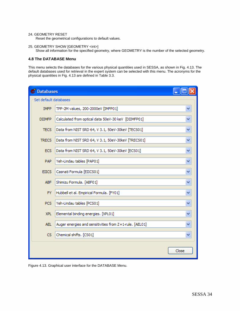
SESSA 34

24. GEOMETRY RESET

Reset the geometrical configurations to default values. 25. GEOMETRY SHOW [GEOMETRY <int>]

Show all information for the specified geometry, where GEOMETRY is the number of the selected geometry.

4.8 The DATABASE Menu This menu selects the databases for the various physical quantities used in SESSA, as shown in Fig. 4.13. The default databases used for retrieval in the expert system can be selected with this menu. The acronyms for the physical quantities in Fig. 4.13 are defined in Table 3.3.

Figure 4.13. Graphical user interface for the DATABASE Menu.

SESSA 35


1. DATABASE IMFP SET <string>

Select a database for retrieval of inelastic mean free path (IMFP) values. 2. DATABASE IMFP SHOW

Show a list of available databases for the IMFP in the CLI.

3. DATABASE DIIMFP SET <string> Select a database for retrieval of the differential inverse inelastic mean free path (DIIMFP).

4. DATABASE DIIMFP SHOW

Show a list of available databases for the DIIMFP in the CLI. 5. DATABASE TECS SET <string>

Select a database for retrieval of the total elastic cross section (TECS). 6. DATABASE TECS SHOW

Show a list of available databases for the TECS in the CLI. 7. DATABASE TRECS SET <string>

Select a database for retrieval of the transport (elastic) cross section (TRECS). 8. DATABASE TRECS SHOW

Show a list of available databases for the TRECS in the CLI. 9. DATABASE ECS SET <string>

Select a database for retrieval of the (differential) elastic cross section (ECS). 10. DATABASE ECS SHOW

Show a list of available databases for the ECS in the CLI. 11. DATABASE PAP SET <string>

Select a database for retrieval of the photoionization asymmetry parameter (PAP). 12. DATABASE PAP SHOW

Show a list of available databases for the PAP in the CLI.

13. DATABASE PAG SET <string>

Select a database for retrieval of the non-dipolar photoionization asymmetry parameter (PAG) 14. DATABASE PAG SHOW Show a list of available databases for the PAG in the CLI. 15. DATABASE PAD SET <string>

Select a database for retrieval of the non-dipolar photoionization asymmetry parameter (PAD) 16. DATABASE PAD SHOW Show a list of available databases for the PAD in the CLI. 17. DATABASE EIICS SET <string>

Select a database for retrieval of the electron impact ionization cross section (EIICS). 18. DATABASE EIICS SHOW

Show a list of available databases for the EIICS in the CLI. 19. DATABASE ABF SET <string>

Select a database for retrieval of the Auger backscattering factor (ABF). 20. DATABASE ABF SHOW

Show a list of available databases for the ABF in the CLI.

SESSA 36

21. DATABASE FY SET <string> Select a database for retrieval of the fluorescence yield (FY).

22. DATABASE FY SHOW

Show a list of available databases for the FY in the CLI. 23. DATABASE PCS SET <string>

Select a database for retrieval of the photoionization cross section (PCS). 24. DATABASE PCS SHOW

Show a list of available databases for the PCS in the CLI. 25. DATABASE XPL SET <string>

Select a database for retrieval of the X-ray photoelectron lineshape (XPL). 26. DATABASE XPL SHOW

Show a list of available databases for the XPL in the CLI. 27. DATABASE AEL SET <string>

Select a database for retrieval of the Auger electron lineshape (AEL).

28. DATABASE AEL SHOW Show a list of available databases for the AEL in the CLI.

29. DATABASE CS SET <string> Select a database for retrieval of the chemical shifts. 30. DATABASE CS SHOW Show a list of available databases for chemical shifts in the CLI. 31. DATABASE SHOW DATABASE

Show a list of the databases selected for retrieval/simulation of XPS/AES spectra in the CLI.

4.9 The SIMULATION Menu This menu controls parameters of the simulation, as indicated in Fig. 4.14. SESSA is able to perform a Monte Carlo simulation of an electron spectrum based on the parameters retrieved for the specified sample and for the specified experimental conditions, as described in Ref. [1]. For this purpose, a number of trajectories that mimic the physics of the electron transport are generated. The simulation algorithm is very efficient: each trajectory contributes to all energies in the spectrum. This is achieved by assigning an a posteriori likelihood for n-fold scattering to each trajectory. For each trajectory, a contribution to the so-called partial intensities is calculated. These quantities represent the probability that a given electron arrives at the detector after experiencing a given number of collisions. Multiplying this number with the distribution of energy losses after a given number of inelastic collisions gives the partial spectrum of n-fold inelastically scattered electrons. Adding up these contributions gives the total simulated spectrum. Furthermore, the trajectory reversal algorithm [8] is used by SESSA. This algorithm allows a user to perform simulations for a detector with an infinitely narrow opening angle of the analyzer; see Ref. [1] for more details about the simulation procedure. The maximum number of inelastic collisions ("Number of collisions") is either determined automatically or can be set by the user. The computation time required for a simulation increases with this maximum number, in particular if ndiimfp = 2 is chosen in the preferences menu (see section 4.3). If only the intensities of the peaks in the

spectrum are of interest (electrons escaping without any inelastic collision), the maximum number of collisions can be set to zero. The simulated spectral shape will then be unrealistic, but the peak intensities will be realistic and generated very efficiently. The number of trajectories that is generated is either determined automatically by the convergence criterion, or can be specified by the user (typically 500 for a calculation with 1 % precision). For illustrative purposes, the user may wish to carry out simulations in various approximations. It is presently possible to choose between three different approaches obtained by employing different distributions of scattering angles and associated mean free paths for successive collisions:

SESSA 37

Figure 4.14. Graphical user interface for the SIMULATION Menu. (1) the usual "Mott" cross section for elastic scattering calculated from the relativistic plane-wave expansion method that is believed to provide a realistic description of elastic-scattering events of electrons in solids when used in conjunction with the elastic mean free path derived from it [9, 10]; (2) neglect of elastic deflections (straight line approximation, SLA, or rectilinear motion model), corresponding to an infinite elastic mean free path; and (3) an isotropic transport cross section taking the transport mean free path as the characteristic length for elastic deflections. The latter approach is essentially equivalent to the so-called transport approximation (TA) [1, 11]. The latter two options for the simulation approach can be selected by checking the corresponding boxes labeled Straight Line and Transport in the GUI (Fig. 4.14). The Show peak intensities and Save peak intensities buttons provide a convenient means of displaying and/or saving the zero-th order partial intensities for the peaks in the spectrum. These operations (that are available for all partial intensities) can also be performed from the Sample Peaks screen (Section 4.4.5).

SESSA 38


1. MODEL SET NCOL <int> [REGION <int>]

Set the maximum number of inelastic collisions to a fixed value, where REGION is the number of the selected spectrometer region.

2. MODEL SET NTRAJ <int> [REGION <int>]

Set number of trajectories used in the simulation to a fixed value, where REGION is the number of the selected spectrometer region.

3. MODEL SET TA <string>

Set TA (transport approximation) to true or false. If TA is set to true, an isotropic distribution of polar deflection angles for elastic scattering is used in the simulation.

4. MODEL SET SLA <string>

Set SLA (straight line approximation) to true or false. If SLA is set to true, elastic scattering of the signal electrons in the sample is neglected.

5. MODEL SET CONVERGENCE <double>

Set the convergence criterion for the MC simulation. The simulation for a given peak terminates when the relative change in the sum of all requested partial intensities drops below the criterion for ten successive trajectories. So, for example, if the user has set number of collisions = 0, and the convergence criterion is

0.01, then the simulation terminates if the intensity of the no-loss peak changes by less than 1% for 10 successive trajectories. The precision of the calculation for the peak intensity will then be better than 1%. Note

that when an entire spectrum is simulated (number of collisions<>0), the sum of all partial intensities (to

which the termination criterion applies) is actually the total spectral intensity (area under the spectrum) for the considered transition.

6. MODEL SET WRITETRAJ <string> If the variable WRITETRAJ is ’true’, individual trajectories are written to disk. The filename can be controlled by the command ’model set TRAJFILE’. The extension ‘trj’ will be added to the file name itraj_ipeak_igeo.trj where ’itraj’, ’ipeak’ and ’igeo’ are the number of the trajectory, the peak, and the geometry. If more than one spectrometer region is specified, the resulting trajectory files will correspond to the last spectrometer region simulated (i.e., the one with the highest number). Each file consists of 6 columns. The first three columns give x-, y- and z-coordinates of the particle position at an elastic-scattering event, at the boundary between regions with different materials, or at the boundary of a nanostructure on the surface (i.e., the nanostructure-vacuum interface). The final three columns give the same coordinate positions for an elastic-scattering event in a single nanostructure (i.e., a nanostructure that does not have periodicity). While a SESSA user can change the periodicity of a selected nanomorphology, the effects of the periodicity can be distinguished even when the period is large. Note that the positive z-axis is orientated along the sample-surface normal pointing into the sample. The computation speed also decreases dramatically if WRITETRAJ is activated. It is suggested that the number of trajectories in the Model menu should be set to a reasonable value; between 10 and 50 trajectories are usually more than sufficient for visualizing the transport.

7. MODEL SET TRAJFILE <string> Sets the name of the file (and directory) to which the trajectory information is written using the command ’model set writetraj’.

8. MODEL SET SINGLE <string> If this parameter is ’true’, simulation of a single nanoparticle on the surface is performed instead of a periodic array of nanoparticles.

9. MODEL AUTO NCOL [REGION <int>]

Maximum number of inelastic collisions will be automatically calculated by the simulation module, where REGION is the number of the selected spectrometer region.

10. MODEL AUTO NTRAJ [REGION <int>]

Number of trajectories will be automatically calculated by the simulation module, where REGION is the number of the selected spectrometer region.

SESSA 39

11. MODEL PLOT [REGION <int>] Graphical representation of the simulated spectrum for a given spectrometer region in the separate plot window, where REGION is the number of the selected spectrometer region.

12. MODEL SIMULATE

Perform a Monte Carlo simulation of the spectral shape using the given settings for all relevant parameters. 13. MODEL SHOW

Show information on parameters controlling the simulation.

5 RETRIEVAL STRATEGY AND SIMULATION MODEL

5.1 Retrieval strategy of the expert system In a first step, the expert system establishes the relevant peaks in accordance with the user's specification of the sample composition and the selected excitation source and spectrometer settings. This is done by looking up the source energy and the type of exciting radiation (photons, electrons) and querying the databases for the peak shapes for each element in all layers of the sample. When a peak is found that is not present in the internal peak list, and falls within any of the specified spectrometer regions, the peak is added to the peak list. This peak list is on display in the "Sample/Peaks" menu in the GUI and can be listed via the corresponding command in the CLI. The energy distribution for a useful peak in an AES or XPS spectrum for a solid is known to be sharply peaked with respect to the nearby background. However, the total energy range where the emission probability assumes non-vanishing values can generally be very broad. In order to decide whether a peak should be taken into account in a given spectrometer region, it is therefore necessary to invoke some meaningful criterion. In the SESSA expert system this is done by comparing the fraction of the peak area that falls within the considered spectrometer energy region with the threshold parameter. If this fraction exceeds the threshold value specified by the user (see Section 4.3), the peak is included; otherwise it is discarded from the peak list. If a given element is present in more than one chemical state, each peak for this material is added in duplicate to the peak list, and is accordingly labeled. While the main purpose of the chemical-state label is indeed to indicate the chemical states of a given element in order for the software to be able to differentiate between them, it is to be noted that the chemical state label is nothing but an arbitrary label allowing such a distinction to be made. In other words, it can just as well be used for an entirely different purpose, e.g., to simulate the excitation depth distribution in some special applications of electron spectroscopy (see, for example, Section 7.3.1). After the relevant peaks have been established in this way, the parameters for the generation of the associated signal electrons are retrieved from the corresponding databases together with the parameters describing the characteristics of the electron-solid interaction (or, in other words, the surface sensitivity) are obtained from the relevant databases. As mentioned before, an essential aspect of the expert system, in particular in conjunction with a simulation module, is that for each considered electronic transition leading to the emission of signal electrons, all parameters concerning their generation and interaction with the solid must be known; otherwise the software will eventually be unable to take

meaningful decisions and to provide meaningful results (i.e., the software would cease to run). This situation is, of course, completely unacceptable, and the databases must therefore be able to return at least a credible estimate for each queried quantity. As explained in Section 3.1, SESSA is designed always to provide a backup database that is extensive. The reliability of the returned datum from the backup database is, of necessity, not always comparable to the typical reliability of the other databases. Nevertheless, the fact that each datum is traceable to its source in the scientific literature (see also Section 6) makes the individual reliability of any datum accessible to the user, while the overall reliability of, for example, the outcome of a simulation of SESSA can be assessed in survey form by inspection of the files ending with rems.txt and refs.txt (see Section 3.4).

5.2 Algorithm for spectrum simulation When all needed parameters have been retrieved from the databases, a simulation of the expected outcome of the specified experiment can be performed with SESSA. The simulation algorithm is based on the partial intensity approach for the electron-solid interaction [1, 12, 13,14, 15]. The key quantities in this approach are the so-called partial intensities that describe the number of electrons arriving at the detector after having participated in a given number of inelastic collisions in the solid between their point of generation and escape from the surface. In SESSA, the partial intensities are calculated with a very efficient Monte Carlo calculation based on the so-called trajectory reversal algorithm [8] that benefits from a symmetry property of the (linearized) Boltzmann kinetic equation which forms the basis of the surface sensitivity of electron-beam techniques for non-crystalline solids. In the following

SESSA 40

sections, the simulation algorithm is described in some detail in order for a user to be able to understand and interpret the results of a simulation. In the range of medium energies (50 eV to 20 keV) for which SESSA is designed, the characteristics of the electron-solid interaction allow some drastic simplifications to be made leading to a convenient starting point of the theory. In particular, a clear distinction can be made between multiple inelastic scattering and multiple elastic scattering. While inelastic scattering can be treated in a straightforward manner by means of an analytic theory, elastic scattering is most conveniently tackled by means of a numerical approach. The Monte Carlo technique employed by SESSA is the most flexible numerical technique with respect to the boundary conditions of the considered problem. 5.2.1 The electron spectrum in AES/XPS

The objective of SESSA is to facilitate interpretation of the spectra of electrons that are generated by means of electron or photon bombardment in the near -surface region of a solid, escape from the surface, and are analyzed and detected by a spectrometer. Obviously, the quantities relevant for the relevant processes and, in particular, any eventual relationship between them need to be studied before establishing a theory describing the phenomenon. A detailed discussion of the physical quantities describing signal-electron generation and transport is beyond the scope of this Guide, and the reader is referred to reviews in the literature (e.g., Refs. [1, 16, 17]).

The most important facts may be summarized as follows:

For any given electronic transition, the energy and angular distributions are uncorrelated; i.e., the energy distribution of electrons liberated at an atom in a solid is the same for all emission directions. Since the depth distribution of the emitting sources is determined by the compositional depth profile of the specimen, we expect

that the source angular, energy and depth distributions will be uncorrelated. The source distribution ),,(0 zES

can then be factored into energy- ))(( 0 Ef , angular- ))(( 0 g , and depth- ))(( 0 zc dependent terms:

)()()(),,( 0000 zcgEfzES (5.1)

Here ),( is a shorthand notation for the electron emission direction, specified by the polar angle and

the azimuthal angle .

The electron-solid-interaction characteristics for the electron transport (mean free paths, cross sections, etc.) are not strongly dependent on energy. More precisely, the change in any interaction characteristic is small compared

to the value of that quantity when the energy changes by an amount E corresponding to a typical energy loss

2.27/ 02 aeT eV in an inelastic collision, where e is the electronic charge and a0 is the Bohr radius. We

then have:

T

E

(5.2)

where stands for any of the interaction characteristics.

The width of the energy distribution for a useful peak in an AES or XPS spectrum is small compared to the typical energy loss in an inelastic collision.

Energy losses and deflections can be regarded as independent processes. The above conditions are generally fulfilled in AES and XPS [1] and allow one to immediately understand the so-called partial intensity approach for the theoretical description of an electron spectrum, without resorting to complicated mathematical derivations. Readers interested in a rigorous mathematical treatment of the problem are referred to Ref. [17]. It is obvious that each electron leaving the surface has experienced a given number, say n = 0, 1, 2, … , of inelastic collisions. In other words, the emerging spectrum consists of groups of electrons that have experienced a certain

number of inelastic processes. Since the energy and angular distributions in the source function ),,(0 zES

SESSA 41

factorize into energy and angular terms, and since elastic (deflections) and inelastic collisions (energy losses) may be assumed to occur independently, it follows that each of the groups of n-fold inelastically scattered electrons is also a

product of a function )(EFn depending only on the energy and a function )(nC that depends only on the emission

direction. Taking the energy distribution of the n-th group, the so-called partial energy distribution, to be normalized,

1)( dEEFn , the partial intensities )(nC are identified as the number of electrons in the corresponding group.

Since the energy dependence is assumed to be sufficiently weak, it follows that the interaction characteristics within each group can be taken to be the same and, furthermore, since the energy distribution at the source is narrow compared to the typical energy loss, the transfer processes determining the surface sensitivity are the same for all electrons within a given peak.

Summing up the different groups gives the spectrum ),( EY :

)()(),(max

0

EFCEY n

n

nn

(5.3)

In this expression, nmax is the largest order of inelastic scattering considered. In SESSA, this parameter can be

automatically determined, by clicking the Auto box in front of the "number of inelastic collisions" field in the Simulation menu, or it can be set by the user. The latter option is convenient, e.g., when only the intensity of the peak of no-loss electrons is of interest since this intensity can then be calculated very efficiently (see Section 5.2.3). The remaining problem is to find a convenient means of evaluating the partial energy and intensity distributions, as described in the next two Sections. 5.2.2 Multiple inelastic scattering: the partial energy distributions

Since the transport equation is linear, it is straightforward to express the distribution of energy losses after a given

number of inelastic collisions in terms of the source energy distribution )(0 Ef if the energy-loss distribution in a

single inelastic collision )(Tw is known. The latter quantity is, of course, identical to the (normalized) differential

inelastic inverse mean free path for which a database is available in SESSA.

Let us assume that the source energy distribution )(0 Ef is normalized to unity area. The probability that an Auger-

electron or photoelectron is emitted by an atom in the sample with an energy between TE and dTTE is then

given by dTTEf )(0 . Multiplying this probability with the probability for an energy loss in the interval ),( dTTT

gives the probability that the electron has the energy E after experiencing a single inelastic collision. Integrating over all different possible values of the energy loss T gives the energy distribution after one energy loss as:

dTTwTEfEF )()()( 01 . (5.4)

In exactly the same way, the higher-order loss distributions may be calculated. The whole procedure may be summarized by the recurrence relations:

dTTwTEFEF nn )()()( 1

dTTLTEf n )()( 10 . (5.5)

In the second line of this equation, the partial loss distributions )(TLn , i.e., the distribution of energy losses after n

inelastic collisions, is introduced. When more than one inelastic-scattering distribution is of relevance for the considered problem (e.g., when the inelastic-scattering properties are significantly different in the two topmost layers of the sample), the above equations can be generalized as follows:

dTTwTEFEF nnnnnn )()()( 1,...3,2,11,...3,2,1

SESSA 42

dTTwTEF nnn )()( 2,...3,12,1 …, (5.6)

where )(1 Tw is the distribution of energy losses for the first layer, etc. In the present version of SESSA, it is possible

to distinguish between two different inelastic-scattering distributions, )(1 Tw and )(2 Tw , by setting the parameter

NDIIMFP to two. One inelastic-scattering distribution ( )(Tw ) is set as the default (NDIIMFP=1) (see Section 4.3).

5.2.3 Multiple elastic scattering: the partial intensities

The partial intensities ),( einC , i.e., the number of signal electrons arriving at the detector, depend on several

experimental parameters such as the flux of exciting radiation, the spectrometer transmission etc., as well as on the

source depth distribution of the emitting species )(0 zc (where )(0 zc represents the atomic fraction of an element at

a given depth z), the probability that a transition takes place at a certain depth, the so-called excitation depth

distribution function ),,( xix z , and the probability for escape after n inelastic collisions that is described by the

emission depth distribution function ),,(, exne z :

)(),,(),( 0

4 0

zczDAFTNC xixaein

exexne ddzdz ),,(, . (5.7)

The subscripts x and e are used here to denote the excitation and emission processes, respectively, and x and

e are the emission directions of the signal electrons at the source and after emission from the surface. In Eq. (5.7),

D denotes the detector efficiency, T is the spectrometer transmission, F is the flux of the exciting radiation, Na is the atomic density, and A is the analyzed area. The latter variable is obviously determined by the experimental geometry

and, in particular, depends on whether the area seen by the analyzer exceeds the excitation area on the sample. In this case, the analyzed area is independent of the emission angle, whereas for the opposite case when the illuminated area is much larger than the area seen by the analyzer, the analyzed area varies with the polar emission

angle as eA cos/1 . The latter situation corresponds to the XPS mode in the Geometry menu of SESSA (see

Section 4.7) while the former corresponds to the AES mode; note, however, that the AES mode could be applicable to XPS instruments in which the incident X-rays are focused to a relatively small area. It is also important to recognize that perfect alignment of the beam of primary radiation and the analyzer is not always achievable in measurements of angular distributions, in which case geometrical artifacts can arise in the measured angular distributions. Sometimes, measurements can be made of the relevant calibration factors. These calibration factors, if known, can be entered for a given geometry in the geometry correction factor box of the Geometry menu.

The term in Eq. (5.7) represents the solid angle of acceptance of the analyzer over which the emitted spectrum needs to be integrated. The magnitude of the acceptance solid angle is indicated in the Geometry menu by specifying

the upper and lower values of the polar and azimuthal angles ( and ). The factors D, F, and T in front of the

integrals in Eq. (5.7) are taken to be unity in the present implementation of SESSA. A further simplifying assumption made in the simulation is that the excitation depth distribution function

),,( xix z varies only very slowly with depth. This quantity can then be taken outside the depth integral and

replaced by the electron-production cross section ),( xiex . In an XPS experiment this production cross section

is equal to the photoionization cross section ),( xiph . In AES, the production cross section is independent of

x and is given by the product of the electron-impact ionization cross section ei and the Auger backscattering

factor ))(1( iAr , that accounts for the additional ionization of the considered subshell through backscattered

primary electrons, and the probability that the core hole is filled via the considered Auger electron transition, indicated

here with A so that ))(1( iAAeiex r . In the present version of SESSA, the angular dependence of the

excitation depth distribution is also simplified. In the case of AES, the dependence on i is assumed to follow

SESSA 43

Shimizu's expression [18], while the emission angular distribution at the source is taken to be isotropic. For XPS, it is assumed that the direction of incidence at the location of signal-electron generation is identical to the incident direction of the X-rays on the surface, i.e., deflections of photons in the solid and at the surface are neglected. Taking into account the above assumptions and collecting all constant terms into a new constant K, the partial intensities can be written as:

eieinexiexein ddzdzzcKC

),,()(),(),( ,0

4 0

, (5.8)

where ),( xiex represents the normalized angular part of the production cross section.

The emission depth distribution function ),,(, xine z represents the probability for signal-electron escape from a

given depth after experiencing a given number n of inelastic collisions. The probability for n-fold scattering, on the other hand, depends on the electron pathlength inside the solid. Due to elastic scattering, not all electrons travel the

same pathlength; instead, the pathlengths s are distributed according to a function ),,,( exszQ . In other words,

the depth distribution function can be expressed in terms of this pathlength distribution function and the probability for

n-fold scattering as a function of the traveled pathlength )(sWn [12]; the latter function is given by the Poisson

distribution when the interaction characteristics are assumed to be independent of the energy. The latter approach, known as the quasi-elastic approximation [1, 12, 16, 19], is adopted in SESSA and is valid when the considered energy-loss range is small compared to the signal-electron energy. The emission depth distribution can be written as:

dssWszQz nexexne )(),,,(),,(

0

,

. (5.9)

Using this result, Eq. (5.8) can be transformed as follows:

),,,()(),(),( 0

4 0 0

exxiexein zsQzcKC

dsddzdsW ein )( . (5.10)

The distribution of pathlengths represents a quantity that is ideally suited for calculation with the Monte Carlo (MC) technique since, with this approach, a large set of trajectories is simulated. By making a histogram of the lengths of such a set of trajectories, the pathlength distribution is immediately obtained. In SESSA, the integral in Eq. (5.10) is therefore calculated by means of the MC technique. The MC simulation is based on the very efficient trajectory reversal algorithm [8] which in turn is based on a symmetry property of the Boltzmann kinetic equation, the so-called reciprocity theorem (see e.g., Ref. [20]). This theorem states that, for a quasi-elastic trajectory, the source point and the termination point of a trajectory are equivalent. In other words, instead of simulating a trajectory from its source point through the solid and hoping that this electron is emitted from the surface with the correct direction to be detected by the analyzer (which, depending on the magnitude of the acceptance solid angle of the analyzer, is not likely to be the case for the overwhelming majority of all trajectories), one can also start the simulation at the analyzer and trace back the path of the electron inside the solid. In this way, a significant increase in efficiency of an MC calculation is obtained that makes it possible to perform simulations of this kind on a personal computer. The generation of trajectories proceeds in the usual way by means of the Monte Carlo technique. More details can be found in Ref. [1]. The user has a choice among three different types of elastic-scattering cross sections for a simulation: 1. The "Mott" cross section for elastic scattering derived from the relativistic plane-wave expansion method. This

choice is believed to give the most reliable results [62], and is recommended for most applications. 2. The isotropic transport cross section. This choice (made by checking the Transport box in the Model menu of

Fig. 4.12) allows a faster simulation of the trajectories and gives excellent results when the conditions of the so-called generalized radiative field principle are met [11]. The use of the transport cross section corresponds to making the transport approximation that is often used in the analytic treatment of such problems [1]. The transport cross section is one of a few types of cross section for which the transport equation can be solved analytically.

SESSA 44

3. A forward-peaked delta-function-shaped "cross section" representing the rectilinear-motion model or straight-line approximation (SLA). This choice (made by checking the Straight Line box in the Model menu of Fig. 4.14) allows a user to study the magnitude of elastic-scattering effects in a given application (i.e., by comparing results from this choice with results of a similar simulation made using the Mott cross section).

In SESSA, the efficiency of the trajectory-reversal algorithm is further enhanced by directly calculating the partial intensities, rather than first calculating the pathlength distribution and then integrating this distribution. Furthermore, the method of statistical weights is used to account for the angular and depth dependences of the source function. To appreciate the former statement, note that the integrals in Eq. (5.9) and Eq. (5.10) can be calculated immediately along each trajectory, instead of first making a histogram and then later performing the integrations. The integral in

Eq. (5.10) can thus be solved by directly summing the contributions to the partial intensities knC )( corresponding

to the k-th linear step between two deflections in the MC algorithm as follows:

dsszcsWkC kxiex

ss

s

neikn

kk

k

))((),()(),()( 0,

. (5.11)

Here sk is the pathlength traveled in the solid before the k-th step and ks is the length of the k-th step. The second

and third factors in the integral account for the angular and depth dependences of the source function. Assigning the appropriate weight factors for the source distribution in this way in an MC algorithm is known as the method of statistical weights. The integral in Eq. (5.11) can be evaluated analytically, leading to an additional enhancement of computational speed. After a sufficiently large set of trajectories has been obtained in this way, the partial intensities are finally obtained as:

),()(1

),( ,0 0

eijk

N

j

N

kn

traj

ein

traj k

CN

C

, (5.12)

where Ntraj is the number of trajectories and Nk is the number of steps per trajectory. The value of Nk is determined by the termination criterion. When the total pathlength of a trajectory exceeds a pathlength given by the following

function of the inelastic mean free path and the order of partial intensities nmax considered,

)5(2 max ns i , (5.13)

the trajectory is terminated. The total number of trajectories, Ntraj, in Eq. (5.12) is determined by the convergence criterion. If the fractional change of the sum of all considered partial intensities is below the convergence factor (provided in the Model menu of Fig. 4.14), generation of trajectories is terminated. The sum of all partial intensities is, of course, identical to the total spectral intensity of a peak (i.e., the area of the peak and its associated inelastic background). Note that for the case of a thin layer on a substrate, the partial intensities decrease rapidly with the order of inelastic scattering. On a logarithmic display, the dependence of the simulated partial intensities on the number of inelastic collisions may then exhibit oscillations. These oscillations are caused by the fact that the higher-order partial intensities contribute only negligibly to the total spectral intensity; these oscillations are thus an artifact of the convergence of the simulation. As an alternative means to control the convergence behavior of the algorithm, the user may directly specify the number of trajectories in the Model menu of Fig. 4.14. A convergence factor of 0.01 will be satisfactory for many applications. A final aspect of the simulation that should be mentioned here is the fact that the vacuum-solid interface is generally assumed to be atomically flat in SESSA. The only other surface morphology, apart from this idealized concept of an atomically flat surface, is a rough surface. The surface roughness can be specified by a user in SESSA by setting the value of the relative surface area (RSA) in the Sample menu of Fig. 4.5. The RSA is a measure for the surface roughness in terms of the ratio of the real surface area divided by the projected surface area, i.e., the area of the idealized flat surface. 5.2.4 Modeling of nanostructured surfaces in SESSA

There are generally three aspects of the photoelectron (or Auger-electron) emission process that can be affected by the nanomorphology of a surface:

SESSA 45

1. The photoionization process itself may be different from that for an ideal flat surface. The intrinsic peak shape, i.e., the energy distribution of the photoelectrons directly after photoionization, could be modified due to possible differences in the screening response in the local region compared to a semi-infinite surface.

2. The inelastic-scattering processes near the surface may exhibit additional modes related to the morphology and

composition of a nanostructured surface [24].

3. The distribution of pathlengths of specific photoelectrons created in a material A that travel in another material, say B, depends on the geometric boundaries of the considered morphology. As a consequence, the relative peak intensities (and the shape of the inelastic background) will be influenced by inelastic scattering along the trajectory and can also be affected by the morphology and composition of the nanostructure.

Some evidence for the existence of nano-structure-induced changes in the photoelectron peak shape exists, but are not included in the present version of the software. It should be noted that, even for planar surfaces, the intrinsic peak shapes used for spectrum modeling are not generally realistic; they are assumed to be a single Lorentzian with a width of 0.7 eV by default. However, more realistic peak shapes can be imported using empirical data from a text file (see Section 4.4.7). This strategy should work equally well in simulation for nanostructured surfaces. The additional modes of inelastic-scattering processes near nanostructured surfaces are obviously of paramount importance for the optical properties of nanostructures and their study has become an important subfield of nanophotonics and plasmonics [24]. Such modes can most easily be studied by electron energy-loss spectroscopy (EELS) in the transmission electron microscope (TEM) and can be observed in EELS spectra as clearly distinguishable features extending from the near infrared to the near ultraviolet regime of wavelengths. However, on the scale of loss features important for understanding the attenuation of photoelectrons, these effects are believed to be of minor importance and are in fact expected to be nearly impossible to detect in typical XPS spectra. The reason is that the overwhelming majority of processes attenuating the outgoing photoelectrons (and thereby affecting the relative intensities, extrinsic peak shapes, etc.) take place inside the solid, since the surface scattering zone, where additional modes due to the nanomorphology come into play, is at least about an order of magnitude smaller than the relevant mean free paths for inelastic scattering inside the solid. As a result, the most effective experimental means for studying such effects in the TEM is to use an aloof scattering geometry in which the beam does not actually penetrate the specimen; alternatively, a supporting substrate that is (almost) completely transparent to the beam (such as mica) can be used. With these techniques, inelastic scattering inside the solid can be minimized and the spectral features of interest can be observed. For simulation of nanostructured surfaces with SESSA, one has just the opposite situation since the signal always originates from within the surface, making the phenomena addressed above difficult to distinguish in experimental spectra. On the other hand, theoretically explaining such spectral features is very difficult in general: one either has to resort to semi-classical theories or to full quantum-mechanical treatment of the many-body problem involving the nearly free solid-state electrons [29,30]. This type of analysis is obviously beyond the scope of general-purpose software such as SESSA. Moreover, since these effects are expected to weak in photoelectron spectra, they are not incorporated in the present version of SESSA. The spatial distribution of matter (i.e., the three-dimensional geometric distribution of matter inside a sample) near a nanostructured surface is known to have a major effect on features of the energy and angular distributions of emitted photoelectrons [31,72,73]. This result is not surprising since typical dimensions of nanostructures are of the same order as the inelastic mean free paths of the detected photoelectrons in typical XPS experiments. It is therefore to be expected that details of the morphology should have a strong effect on the attenuation of photoelectrons in a spectrum and therefore on the relative photoelectron intensities, angular distributions, and inelastic backgrounds. In fact, the influence of morphology on spectra is sometimes so pronounced that significant information on the nanomorphology of a surface can be derived from XPS spectra. The effects of nanostructure morphology is taken into account in the present version of SESSA by keeping track of the pathlengths of electron trajectories within each of the regions of the sample that form the boundary of the nanostructure. With this information, the partial intensities of the relevant peaks in the spectrum are calculated according to the formalism outlined in section 5.2.3.

In the present implementation of SESSA, the nanomorphology of the surface is defined and traced using the

PENGEOM code system [83].3 When a user starts a simulation, the information concerning the nanomorphology of

the surface entered in the SESSA expert system (either using the GUI or the CLI), is written to an internal file,

following the syntax prescribed by the PENGEOM package. This is then used to initialize a PENGEOM data structure

which is used during the simulation to check in which material the electron is located, whether it has crossed a

boundary between two adjacent regions consisting of different materials and to locate the point of intersection. If an

3 The authors would like to thank Prof. F. Salvat-Gavalda (University of Barcelona) for his kind permission to use

the PENELOPE code in SESSA.

SESSA 46

intersection took place, the position of the electron is updated to the location of intersection and simulation of the

trajectory is continued from there in the usual manner.

5.3 Current limitations of databases and simulation It was shown in the previous Section that three quantities need be known for a realistic simulation of the energy and angular distributions: (1) the partial intensities; (2) the source energy, angular and depth distributions; and (3) the differential inelastic inverse mean free path (see Eqs. (5.3) and (5.5)). The additional parameters needed for a simulation of the partial intensities are: the total inelastic mean free path, the differential elastic-scattering cross section, the total elastic-scattering cross section (or, alternatively the transport cross section if the transport approximation is used), the photoionization cross section, the photoionization asymmetry parameter, the electron-impact ionization cross section, the fluorescence yield, and the Auger-electron backscattering factors. For all of these quantities, SESSA contains reasonably reliable data in its databases, while the simulation algorithm for the partial intensities, described above, has also proven satisfactory. Comparisons of peak intensities with experimental results exhibit close agreement (see Sections 7.1.1-7.1.4). This situation is generally the case for the intensity of those electrons that escape without being inelastically scattered. It should be emphasized again that the area of the no-loss peak is identical to the zero-order partial intensity, while the higher-order partial intensities describe the spectral intensity in the inelastic background. For the distribution of energy losses in an inelastic process (i.e., the differential inverse inelastic mean free path), there exists a limited number of materials for which optical data are available that allow a detailed calculation of this quantity. For all other materials, Tougaard's universal cross section is used as a backup data source that gives a reasonable estimate of the overall shape of the loss distribution, but does not describe the fine details of the inelastic excitation probability of a solid. Furthermore, surface and intrinsic excitations [1, 16] are entirely neglected in the present version of SESSA. The main limitation in the simulation of the spectral shape (as opposed to the spectral intensity) is the fact that the

shape of the energy distribution for inelastic scattering in solids is generally quite complex and a comprehensive database for this quantity, that must be based on empirical data, is presently not available within SESSA nor, for that matter, anywhere else in convenient form. Presently, the lineshape of an XPS peak is approximated. After looking up the specified binding energy in a database for elemental binding energies (containing accepted values for binding energies), a default lineshape is chosen for each peak. This default lineshape is a Lorentzian with a full width at half-maximum (FWHM) of 1.4 eV. For AES, the situation is much more complex, since AES peaks can be very broad and consist of many subpeaks. At present, lineshape information for a limited number of Auger peaks is available in the AEL database in SESSA. The only stored data for these peaks are the kinetic energy of the transition, the subshell where the initial ionization took place, and an empirical sensitivity factor. The latter is needed since extensive knowledge of the probability for emission of the considered Auger electrons requires knowledge not only of the relevant fluorescence yields but also of applicable Coster-Kronig transition probability. Sufficient data for Coster-Kronig probabilities of the needed reliability are not now available. An empirical sensitivity factor is therefore used to estimate the peak intensity of an Auger transition. The lineshape is again chosen by default to be a Lorentzian with a FWHM of 6.0 eV. The default choice of a Lorentzian lineshape is reasonable in many cases for XPS but is hardly ever a realistic choice for an Auger transition. These considerations indicate that a user interested in directly comparing experimental lineshapes with results of a SESSA simulation should provide information on the source energy distribution in the SAMPLE PEAK menu of Fig. 4.7. An example further clarifying this problem is given as a tutorial in Section 7.2.2. Summarizing, the main limitations of the simulation algorithm are that surface and intrinsic excitations are neglected and that the excitation depth distribution function is assumed to be constant inside the specimen. Furthermore, the assumption of an atomically flat surface restricts the applicability of SESSA to practical cases where the surface morphology is not expected to influence the spectral intensities. As far as the databases are concerned, the most important lack of data concerns the empirical peak shapes of photoelectron and Auger-electron transitions and comprehensive data on the Coster-Kronig transition probabilities.

SESSA 47

6 PHYSICAL DATA IN SESSA

A large amount of data is needed to interpret an Auger-electron or photoelectron spectrum quantitatively. The required data include basic physical information on the solid in question (density, atomic number of the constituent atoms, etc.), information on the process of creating the signal electrons (photoelectric effect and Auger-electron emission) as well as the various parameters governing the interaction of the signal electrons with the solid on their way out of the specimen. The number of required physical parameters can therefore be large for a particular situation. The SESSA databases provide an extensive and fully traceable dataset for these parameters. The energy range for which data are available extends from 50 eV up to 20 keV. An extensive dataset for all relevant physical parameters is a strict prerequisite for proper operation of the expert system. On the other hand, it is obvious that not all physical parameters are available for all materials with the same accuracy or, for that matter, are available at all for any arbitrary material. This situation implies that in cases where there are gaps in the data sets, these must be complemented by some credible estimate for the quantity in question. This in turn means that it is generally impossible to make an overall statement on the reliability of the data retrieved by SESSA. It is therefore essential for the data to be fully traceable. Every individual datum retrieved by SESSA is accompanied by a full reference to the literature and in many cases also contains a statement concerning its reliability. The easiest way for the user to assess the overall quality of the retrieved data is to copy these data to disk. Two of the files produced in this way (filenames ending with refs.txt and rems.txt) contain a list with statements

on the reliability of the retrieved data (see Section 3.4). The physical quantities for a particular spectrum generally depend on a number of parameters (material, atomic number, energy, etc.). The range of these parameters for which each quantity is available is determined by the selected choice for the data source. For example, the differential inverse inelastic mean free path (DIIMFP) from optical data can only be provided by Penn's algorithm [21] (which is generally regarded as providing the most reliable results for this quantity) for those materials for which energy-loss functions are available in the literature. However, the backup source for this parameter, Tougaard's empirical DIIMFP [7], provides a universal approximate description for the energy-loss probability in a single inelastic collision. The primary and backup sources for this quantity together are generally extensive in that they cover the entire range of parameters of relevance for AES and XPS. This strategy is generally also followed for other parameters. For each quantity for which the primary (most reliable) source does not completely cover the relevant range, the backup source (usually an approximate empirical expression) is extensive, or vice versa.

6.1 Databases used in SESSA The quantities available in SESSA databases as well as their sources are indicated in the following list. 1. Elemental data (Chemical symbol, chemical name, elemental density (if available), number of valence electrons, atomic weight, atomic electronic configuration, etc.). Source: Refs. [22, 23].

Keys: Material, Atomic number

Range: Atomic Number 1-94 2. Differential inverse inelastic mean free path (DIIMFP) (a) Source: Calculated [74] using linear response theory with the algorithm developed by Penn [21] and using optical data in Refs. [25, 26, 27]

4

Keys: Material, Energy (eV), Energy Loss (eV)

Range: Materials restricted by availability of source data; Energy: 50 eV to 20 keV (b) Source: Universal DIIMFP curve proposed by Tougaard [7]

Keys: Energy Loss (eV)

Range: Universal

4 The authors would like to thank Dr. S. Tanuma (National Institute for Materials Science, Tsukuba, Japan) for

providing his set of optical loss functions for use in SESSA.

SESSA 48

3. Total inelastic mean free path (IMFP) (a) Source: Empirical IMFP expression (TPP-2M) [6, 28]

Keys: Material, Energy (eV)

Range: Material: Universal; Energy: 50 eV to 30 keV (b) Source: IMFP values for 41 elemental solids calculated by Tanuma, Powell and Penn [28] using optical data

Keys: Material ID, Energy (eV)

Range: Material: Restricted to those materials for which optical data are available and IMFPs calculated; Energy: 50 eV to 30 keV 4. Differential elastic-scattering cross section (ECS) a) Source: Values computed by the program of Yates [32] using the relativistic partial-wave expansion method based on atomic Thomas-Fermi-Dirac (TFD) potentials [33, 62]

Keys: Atomic Number, Energy (eV)

Range: Atomic number: 1-99; Energy: 50 eV to 20 keV (b) Source: NIST SRD 64, V 3.1, Electron elastic-scattering cross-section database. Values computed using the relativistic partial wave expansion method based on atomic Dirac-Hartree-Fock (DHF) potentials [62, 67] as used for the NIST Electron Elastic-Scattering Cross-Section Database (SRD 64) [34]. The cross sections obtained from DHF potentials are believed to be more reliable than those obtained from TFD potentials [62].

5

Keys: Atomic Number, Energy (eV).

Range: Atomic number: 1-92; Energy: 50 eV to 20 keV 5. Total elastic-scattering cross section (TECS) (a) Source: Values computed by the program of Yates [32] using the relativistic partial-wave expansion method based on atomic TFD potentials [33, 62]


Range: Atomic number: 1-99; Energy: 50 eV to 20 keV (b) Source: NIST SRD 64, V 3.1, Electron elastic-scattering cross-section database. Values computed using the relativistic partial wave expansion method based on atomic Dirac-Hartree-Fock (DHF) potentials [62, 67] as used for the NIST Electron Elastic-Scattering Cross-Section Database (SRD 64) [34]. The cross sections obtained from DHF potentials are believed to be more reliable than those obtained from TFD potentials [62].

4


Range: Atomic number: 1-92; Energy: 50 eV to 20 keV 6. Transport scattering cross section (TRECS) that is used to determine transport mean free paths (TRMFPs) for simulations using the transport approximation (a) Source: Values computed by the program of Yates [32] using the relativistic partial-wave expansion method based on atomic TFD potentials [33, 62]


Range: Atomic number: 1-99; Energy: 50 eV to 20 keV

5 The authors would like to thank Prof. A. Jablonski (Institute of Physical Chemistry, Polish Academy of Sciences,

Warsaw, Poland) for providing calculated differential elastic-scattering cross sections, total elastic-scattering cross sections, and transport scattering cross sections for use in SESSA.

SESSA 49

(b) Source: NIST SRD 64, V 3.1, Electron elastic-scattering cross-section database. Values computed using the relativistic partial wave expansion method based on atomic Dirac-Hartree-Fock (DHF) potentials [62, 67] as used for the NIST Electron Elastic-Scattering Cross-Section Database (SRD 64) [34]. The cross sections obtained from DHF potentials are believed to be more reliable than those obtained from TFD potentials [62].

4

Atomic Number, Energy (eV)

Range: Atomic number: 1-92; Energy: 50 eV to 20 keV (c) Source: Tilinin's quasi-classical expression [35]


Range: universal 7. Photoionization cross section (PCS)

(a) Source: Values computed by Scofield for Mg and Al K X-rays [36]

Keys: Atomic Number, Subshell ID, Photon Energy (eV)

Range: Atomic number: 1-96; Subshells: extensive; Photon Energy: Mg and Al K X-rays (b) Source: Values computed by the program of Yeh and Lindau [37]


Range: Atomic number: 1-96; Subshells: extensive; Photon Energy: extending from just above the ionization-threshold energy to 20 keV

(c) Source: Values computed by Trzhaskovskaya, Nefedov, and Yarzhemsky [38, 39]

6


Range: Atomic number: 1-99; Subshells: extensive; Photon Energy: extending from just above the ionization-threshold energy to 5 keV above threshold. For higher photon energies, linear extrapolations were made to the calculated values. These extrapolations may introduce an uncertainty of more than 30% in the derived cross sections for energies more than 5 keV above threshold.

8. Photoionization asymmetry parameter (PAP)

(a) Source: Calculations of Reilman et al. [40] for Mg, Al K and Zr M

Keys: Atomic Number, Subshell ID, Photon Energy (eV).

Range: Atomic number: 1-96; Subshells: extensive; Photon Energy: Mg and Al K and Zr M (b) Source: Values computed by the program of Yeh and Lindau [37]


Range: Atomic number: 1-96; Subshells: extensive; Photon Energy: extending from just above the ionization-threshold energy up to 20 keV

(c) Source: Values computed by Trzhaskovskaya, Nefedov, and Yarzhemsky [38, 39]

5


Range: Atomic number: 1-99; Subshells: extensive for atomic numbers ≤ 54 but limited to subshells with binding energies less than 2 keV for atomic numbers ≥ 55; Photon Energy: extending from just above the ionization-threshold energy to 5 keV above threshold. For higher photon energies, linear extrapolations were made to the calculated values. These extrapolations may introduce an uncertainty of more than 30% in the derived asymmetry parameters for energies more than 5 keV above threshold.

6 The authors would like to thank the late Prof. V. I. Nefedov (Institute of General and Inorganic Chemistry, Russian

Academy of Sciences, Moscow, Russia) for providing his calculated photoionization cross sections for use in SESSA.

SESSA 50

It should be noted that the database of Trzhaskovskaya et al. [38,39] is not extensive for some subshells in atoms with atomic numbers ≥ 55. For example, this database might not provide a datum for a certain peak in the considered energy range (as specified by a user through setting the photon energy and the spectrometer energy window). Unfortunately, this database is the only database for non-dipolar asymmetry parameters within SESSA, and the authors know of no other database for these quantities that could avoid this deficiency. There are two possible ways that the expert system could handle such a situation: (1) the expert system could conclude that the information for the peak in question is not complete and therefore decides to delete this peak altogether; or (2) the simulation is performed with neglect of the non-dipolar contribution to the photoelectric cross section. The former alternative is believed to be undesirably restrictive since it does not seem reasonable to delete a peak due to a lack of non-dipolar asymmetry parameters. It would be particularly undesirable to delete a peak arising from

common laboratory x-ray sources (such as Al Kor Mg K) for which the non-dipolar terms are generally small enough for these effects to be neglected. Therefore, the second alternative was adopted in the present version of SESSA, i.e,. the non-dipolar terms are set to zero. Note that no corresponding warning is issued if this occurs. 9. Electron-impact ionization cross section (EIICS) (a) Source: Empirical expression of Casnati et al. [41]

Keys: Atomic Number, Subshell, Electron Energy (eV)

Range: Universal (b) Source: Semiclassical expression of Gryzinski [42]


Range: Universal (c) Source: Empirical expression of Worthington and Tomlin [43]


Range: Universal 10. Photoelectron line shape (XPL). Source: Binding energies of the elements [44].

Keys: Atomic Number, Subshell

Range: Atomic Number, Subshell: extensive 11. Auger electron line shape (AEL). Source: Energies and sensitivities calculated according to the Z+1 rule, as described in the Appendix of Ref. [4].


Range: Atomic Number, Subshell: Limited by availability in data source 12. Fluorescence yield (FY) (a) Source: Polynomial fit to empirical data for K-, L-, and M-shell fluorescence yields by Hubbell et al. [45]


Range: Universal (b) Source: Semi-empirical expression for the K-shell fluorescence yield of Bambynek [46]


Range: Universal (c) Source: Burhop's semi-empirical expression for the K-shell fluorescence yield [47]


Range: Universal

SESSA 51

13. Auger backscattering factor (ABF). Source: Shimizu's formula for normal incidence of an electron beam on a homogeneous solid [48]


Range: Universal 14. Chemical shifts (CS). Source: Measured and calculated chemical shifts from Version 4.0 of the NIST X-ray Photoelectron Spectroscopy Database [68]


Range: Limited by availability of data in source [68]

7 TUTORIALS In the present chapter, a small collection of SESSA CLI-files are presented and discussed. These files should help the reader to get acquainted with the most important features of operating SESSA. In addition, the tutorial sessions might be helpful to better understand some aspects of the surface sensitivity of electron spectroscopy for practical applications. These tutorials consist of a number of files residing in the indicated directories. In each of these directories, there is one file that has the same name as the directory and ends with the extension .ses. Loading this file will perform the tasks specified in all individual files in the directory in one operation. The estimated computation times specified in the sections below are clock times measured when running the simulations on a 1.2 GHz Pentium PC [64].

7.1 Peak Intensities 7.1.1 Angular distribution of photoelectrons emitted from a homogeneous Au sample: Chandrasekhar's H-function

Purpose: Getting acquainted. Performing a calculation of a photoelectron angular distribution and showing a comparison of results arising from different cross sections for elastic scattering.

Time required for simulation: ~ 30 s

Directory: tutorials\au-homo

CLI-files (*.ses): ini.ses, sample.ses, spectr.ses, geo.ses, sla.ses, ta.ses, mott.ses, auhomo.ses

GNUPLOT-files (*.g): compare.g

Output-files (output\*.*): sla_all.adf, ta_all.adf, es_all.adf

Procedure:

1. Start SESSA.

2. Open the CLI-console window (CTRL-9 or choose Project/Command Line Interface from the Main menu). Click on the button Load Session and select the file ...\tutorials\au-homo\ini.ses. SESSA reads a number of commands from this file that initialize the software and sets a few preferences. Press CTRL-p to open the preferences menu. It is seen that the options Output/sample and Output/experiment have been deselected. This means that when SESSA writes output to a file, the corresponding information will not be included (see Section 4.3).

3. Load the file sample.ses and open the "Sample/peak" menu (CTRL-1). It is seen that the sample is now

assumed to consist of a semi-infinite piece of gold. The Sample/peak menu (CTRL-2) displays information on the signal electrons emitted from this sample for the given spectrometer and source settings. The Sample/Parameter"menu (CTRL-3) displays the corresponding parameters describing the electron-solid interaction. A right-mouse click on any of the numbers displayed here allows the user to change the database or view the reference for the value on display. Furthermore, the numbers can be changed by entering any value within a meaningful range. The database selection menu and reference dialog can also be invoked for a graphical representation of the differential elastic-scattering cross section and the differential inverse inelastic mean free path by means of a right mouse click. Furthermore, a double click on

SESSA 52

any of the graphical displays in SESSA transfers their contents to a separate plot window that provides features allowing a user to change the display, to plot the contents of the window to a postscript file, etc.

4. Load the file geo.ses and open the Experiment/geometry menu (CTRL-5). By choosing one out of the

defined eight geometries from the Choose Configuration box, the selected information can be displayed or changed. SESSA will later do a separate calculation for each of the geometrical configurations shown here.

5. Load the file spectr.ses and open the Experiment/spectrometer menu (CTRL-6) to see that the

spectrometer region has been set to a rather narrow energy range. Consequently, only the Au4f7/2 peak is within the spectrometer energy window, as can be verified by pressing CTRL-2. It is seen that the Au4f5/2 peak is also missing and that the asymmetry parameter for the Au4f7/2 peak was set to zero for purpose of a model calculation. This choice was achieved by explicit commands in the file spectr.ses (press CTRL-9

to return to the CLI console and view these commands there).

6. Load the file sla.ses and open the Model Calculation menu (CTRL-7). A peak is on display here and the

Straight Line Approximation box is checked. Furthermore the Auto box for number of collisions is deselected (and ncol is set to zero). The reason for setting ncol to zero is that we are presently only interested in the peak

intensity of electrons that escape without inelastic scattering. By checking the Auto box for number of collisions, an entire spectrum is simulated instead of only the no-loss peak (although the spectrometer range would also have to be extended to lower kinetic energies in order to see any effect). The fact that the Straight Line Approximation box is checked means that SESSA assumes that the paths of the electrons in the solid are straight lines (i.e., elastic scattering of the signal electrons is neglected).

7. Load the file ta.ses and note that the simulation takes longer to converge now. Furthermore, the

Transport Approximation box is now checked instead of the Straight Line Approximation box. This choice implies that elastic scattering is assumed to be isotropic and that the distance between successive elastic deflections is taken to be equal to the transport mean free path. Use of the transport approximation enables an analytic solution to be given for the angular distribution of photoemitted electrons (for emitters homogeneously distributed in a semi-infinite solid): the Chandrasekhar H-function [49]. Whenever the maximum number of collisions is set to zero and more than one geometrical configuration is defined, the partial intensities are displayed as a function of the configuration number (instead of the collision order) in the Sample/peak menu (CTRL-2) when Partial Intensities is selected for graphical display. The partial intensities are seen to decrease monotonically (within the precision of the calculation) when going to more oblique emission. This is the expected behavior for the H-function. To increase the precision of the calculation, decrease the convergence factor in the simulation menu (see Section 4.9).

8. Load the file mott.ses. Another simulation is performed that takes considerably longer. In this simulation,

realistic (Mott) cross sections are used for the differential elastic-scattering cross sections [9, 10, 32-34, 62]. 9. Start GNUPLOT and load the file compare.g. The result should resemble Fig. 7.1.

10. When working with CLI files, the order in which the commands are issued is important. For example, when

sample.ses is loaded after spectr.ses, there will be two peaks in the considered region since the

material is set in sample.ses and the command deleting the peak (and issued before in spectr.ses) will

therefore be overruled. For user convenience, a file au-homo.ses has been included that runs all tests

described in this section and should lead to the result shown in Fig. 7.1.

Discussion: The results shown in Fig. 7.1 provide a test for correct operation of a Monte Carlo simulation of electron transport in that the Chandrasekhar function represents the exact analytic solution of the emission problem for isotropic sources in a semi-infinite homogeneous medium and isotropic scattering. The H-function may be approximated by

)1(31

31),(

H (7.1)

In this expression, cos , when is the electron emission angle with respect to the surface normal and is the

single scattering albedo given in terms of the inelastic (i) and transport (tr) mean free paths as )/( trii .

The test is seen to be successful for SESSA. It is furthermore seen that the difference with the more realistic Mott

SESSA 53

cross section is not very significant. This result is explained by the so-called generalized radiative-field similarity principle [11] that specifies conditions for this similarity between isotropic and non-isotropic scattering to occur. It is also seen that the intensity at normal emission is decreased compared to the rectilinear-motion model where elastic deflections are completely neglected (SLA, Straight Line Approximation). See Ref. [50] for a more detailed discussion.

Figure 7.1. Angular distribution of the Au 4f7/2 photoelectron peak intensity excited by Al K X-rays as a function of the polar emission angle (that is, as the sample is tilted). For model purposes, the photoionization asymmetry parameter was set to zero (isotropic emission). It can be seen from the open symbols that the SESSA results obtained in the transport approximation coincide with Chandrasekhar's H-function [49] represented by the solid line. This result is expected since the H-function is the exact analytic distribution for isotropic scattering. The solid circles show results from SESSA in which realistic (Mott) elastic-scattering cross sections were used. The dashed line shows results from the straight-line approximation (SLA) in which elastic scattering is neglected. 7.1.2 Angle-resolved XPS for a homogeneous Al sample

Purpose: Examine the effects of elastic scattering and of the acceptance solid angle of the analyzer


Directory: tutorials\al-anisotropy

CLI-files (*.ses): ini.ses, sample.ses, spectr.ses, geo.ses, sim.ses, al-anisotropy.ses, infinite.ses


Output-files (output\*.*): sla_all.adf, ta_all.adf, es_all.adf

Procedure: The only difference from the procedure of Section 7.1.1 is that the three simulation steps are now executed in one file (sim.ses). The difference in the calculations is that the anisotropy of the photoionization cross section is not

switched off: on the contrary, it is of main interest here. The specified geometries correspond to perpendicular irradiation of the back of a thin Al foil; the analyzer is again rotated around the sample covering a range of polar

SESSA 54

emission angles between -80 and 80o. Note that a polar angle in SESSA is always specified by a positive number in

the range 0o to 180

o, as is usual in a spherical coordinate system; "negative" polar emission angles are obtained by

changing the azimuthal angle by 180o (see the file geo.ses for details).

Discussion: When core-level photoelectrons are liberated from an atom, the emitted intensity along the direction of the incident photons vanishes. In solids, however, a finite contribution in the forward direction is always seen. This is illustrated by the open symbols in Fig. 7.2 that represent the experimental data acquired by Baschenko et al. [51]. There are

two reasons why a finite intensity is always observed in the forward and backward directions: first, the acceptance solid angle of the analyzer is finite, and, second, photoelectrons are scattered elastically by atoms in the solid. As a result, the elastic mean free path length may become comparable to the inelastic mean free path. Consequently, the signal electrons are efficiently scattered inside the solid and, even for an infinitely small analyzer acceptance angle, a non-vanishing intensity is expected in the forward and backward directions. The simulation results shown in Fig. 7.2 are consistent with the above interpretation in that, even in the rectilinear-motion model (curve labeled SLA), there is a finite probability for detecting electrons along the surface normal when the analyzer acceptance angle is finite. For an infinitely small acceptance angle, the intensity along the surface normal should be zero in the rectilinear-motion model, but not when elastic scattering is considered. SESSA is able to perform a simulation for an infinitely small acceptance angle of the analyzer by employing a symmetry property of the kinetic equation. Instead of simulating the trajectory from its generation point, tracing it through the solid, and hoping that it is emitted in the direction of the detector, its path is started in the analyzer and traced back in reverse in the solid. In this way, every simulated trajectory contributes to the intensity simulated with the Monte Carlo method. This procedure was devised by Gries and Werner and has become known as "trajectory reversal" [8]. With the conventional MC calculation methods, it is strictly impossible to perform a simulation for an infinitely small acceptance

angle. The reader may load the file infinite.ses to see how long it takes SESSA to converge to the same

precision in such a case. Even for a moderately (but realistically) large polar acceptance angle of 6o, conventional MC

calculations take of the order of weeks to converge to the precision of the data displayed in Fig. 7.2.

Figure 7.2. Ratio of the Al 2s and Al 2p photoelectron intensities as a function of the polar emission angle. Open circles: experimental results of Baschenko et al. [51]. Filled circles: SESSA simulation based on realistic (Mott)

SESSA 55

elastic-scattering cross sections. Dashed line: SESSA simulation based on use of the transport approximation (TA) in which an isotropic transport cross section describes elastic scattering of the photoelectrons. Solid line: SESSA

simulation based on the straight-line approximation (SLA). In the experiment, the excitation was by Al K X-rays that illuminate the back side of a thin Al specimen. In the simulations, a semi-infinite Al specimen was irradiated with Al

K X-rays at normal incidence. The polar acceptance half-angle of the analyzer was 6o. The fact that the analyzer

acceptance angle is finite is responsible for a finite value of the plotted ratio at normal emission in the SLA. 7.1.3 Angle-resolved XPS for an oxidized silicon wafer with a carbon contamination layer

Purpose: Illustrate the concept of chemical-state labeling using an important practical example. Demonstrate that consistency and accuracy of analysis can be considerably enhanced when different factors affecting the measured intensity are all accounted for simultaneously.


Directory: tutorials\sio2-c-arxps

CLI-files (*.ses): ini.ses, sample.ses, peak.ses, geo.ses, sim.ses, sio2-c-arxps.ses


Output-files (output\*.*): sla_all.adf,es_adf.all

Other files: seah.dat

Procedure: 1. Load the file sample.ses and open the Sample/layer menu (CTRL-1). The compositional-depth profile is shown

in the figure in the bottom-right corner. It is seen to consist of three layers: a substrate, a layer consisting of a Si-substrate and O, and a top layer consisting of C. Select the middle layer by clicking on it. This is equivalent to selecting layer 1 in the Choose Layer box in the top-left corner of this menu. It is seen that the Si component of the material constituting this layer is designated as [oxide]. The Si in the substrate has no chemical state attribute (as verified by clicking on the bottom layer). The chemical state attribute is a string of characters that can be freely chosen by the user and is not in any way interpreted by SESSA; it is only used to label the corresponding peaks. Press CTRL-2 to enter the Sample/peak menu to see the effect. Here, the silicon peaks appear double: as plain (elemental) silicon and one labeled as [oxide]. The important point is that these peaks are treated separately in the simulation.

2. Note that the density of the oxide was explicitly set with a corresponding command in the file sample.ses. This

procedure is necessary because SESSA can only estimate the density of compounds, and such estimates may be in error by more than 100%.

3. Load the file peak.ses and open the Sample/peak menu (CTRL-2). It can be seen that different peak energies

have been assigned to the two chemical states of Si: the separation of the peaks facilitates their differentiation in the simulated spectra (but this has no effect whatsoever on the simulated intensities).

4. Load the file geo.ses. 5. Open the Model Calculation menu (CTRL-7) and load the file sim.ses. Go back to the Sample/peak menu,

choose Partial Intensities in the Choose data box of the graphical display, and inspect the result for the Si 2p and Si 2p [oxide] peaks. It is seen that the partial intensities for the two peaks vary differently with polar emission angle. The partial intensity for the substrate Si 2p peak decreases rapidly with increasing polar emission angle (i.e., as the average number of inelastic scattering events increases with increasing pathlength of the signal electrons in the overlayers as the sample is tilted). In contrast, the Si 2p [oxide] partial intensity does not change appreciably with emission angle.

6. Start gnuplot and load the file compare.g. The result should resemble Fig. 7.3.

Discussion: Angle-resolved XPS is an important technique in semiconductor technology for measuring oxide thickness and composition. In principle, the angular distribution of photoelectrons emitted from layered samples carries information

SESSA 56

Figure 7.3. A plot of Y from Eq. 7.2 as a function of cos/1 , where is the electron emission angle, for angle-

resolved XPS experiments with Si 2p photoelectrons from a thin SiO2 film on a Si substrate. Open symbols: experimental data of Seah and White [52]; dashed line: result of SESSA simulations using the straight line-approximation (SLA); solid line: result of SESSA simulations based on Mott cross sections for elastic scattering. on the compositional depth profile. However, there are limits to the amount of information that can be extracted from such data [53]. Experimental data are often analyzed on the basis of an approach in which elastic scattering of the signal electrons is ignored. Within this model, it is found that the intensity ratio of elemental (substrate) silicon and silicon bound to oxygen in a carbon-contaminated Si/SiO2 sample is related to the oxide thickness dox as:

YII

II

L

d

oxsub

suboxox

1lncos

, (7.2)

where L is the attenuation length for Si 2p photoelectrons in the SiO2 film, is the polar emission angle (with respect

to the sample normal), oxI is the Si 2p intensity from the SiO2 overlayer, subI is the Si 2p intensity from

the Si substrate, and oxI and

subI are the corresponding quantities for bulk samples of SiO2 and Si, respectively.

Elastic-scattering effects and other phenomena that are not intrinsically accounted for in the approach of Eq. (7.2) are

sometimes incorporated in the characteristic length L and the value of exsubII . It is clear from Eq. (7.2) that a plot of

Y (based on determinations of the four intensities in the logarithmic term) versus cos/1 will give the oxide

thickness in units of L (if the plot is linear). It can be seen that the open circles in Fig. 7.3 based on the experimental

measurements of Seah and White [52] lie close to a straight line through the origin for 2)cos/1( (i.e., < 60o).

One reason why the analysis based on Eq. (7.2) is so attractive is that the thickness of the carbonaceous contamination layer does not appear in it. In other words, the derived oxide-layer thickness for an arbitrary thickness of any carbonacaeous-contamination layer is independent of the thickness of this layer. On the other hand, for

SESSA 57

emission angles exceeding 60o, the effects of elastic scattering become quite significant, and the experimental points

in Fig. 7.3 then deviate from the straight line expected from Eq. (7.2).

The data of Seah and White in Fig. 7.3 were acquired from experiments with a Si wafer. The results for < 60o were

analyzed with Eq. (7.2) to give a mean SiO2 thickness of 39 Å. Figure 7.3 shows SESSA results based on the Mott elastic-scattering cross section (solid line) and on the straight-line approximation (SLA) (dashed line). These results were obtained for a 36 Å oxide layer that gave the best consistency between the solid line and the experimental results. There is also reasonable agreement between the derived and reported oxide thicknesses. For emission angles exceeding 60

o, the SESSA results with the Mott cross sections show

the expected deviation from the dashed line from the SLA due to the effects of elastic scattering. 7.1.4 Depth distribution function (DDF) in XPS: comparison with experiment

Purpose: Demonstrate that a quantitative model for the surface sensitivity in AES and XPS is implicitly contained in SESSA by comparing results for the Depth Distribution Function (DDF) with experiment.

Time required for simulation: ~ minutes

Directory: tutorials\ag2s-ddf

CLI-files (*.ses): ini.ses, int.ses, mod.ses, mod_sla.ses, ddfini.ses, ddf.ses

Output files (output\*.*): es, sla, esddf, sladdf

Other files: cleanup.bat, ddfcleanup.bat, zemek.txt

Procedure: 1. Load the file ini.ses and open the Sample/layer menu (CTRL-1). If SESSA was started just before loading this

file, a warning is displayed which explains that the density of the compound layer (Ag2S) was only estimated. An appropriate command in the file sample.ses sets the density to a realistic value.

2. Leave the Sample/layer menu open and load the file int.ses. SESSA will perform a simulation of the intensity

of the S 2s line as a function of the thickness of the Ag2S layer. The change of the profile can be watched in the Sample/layer menu during the simulation.

3. Click on the file cleanup.bat (specific to this tutorial) in the ag2s-ddf directory. This operation deletes some

unnecessary files in the output directory and merges the results of the simulation for the zero-order partial intensities into the files es and sla. The latter files contain the peak intensities calculated with SESSA that are

displayed in Fig. 7.4(a).

4. Load the file ddfini.ses and open the Sample/layer menu (CTRL-2). The sample now consists of a 1 Å buried

layer of Ag2S between an Ag substrate and an Ag overlayer. 5. Leave the Sample/layer menu open and load the file ddf.ses. SESSA will perform a simulation of the intensity

of the S 2s line as a function of the thickness of the Ag overlayer covering the 1 Å buried Ag2S layer. The corresponding S 2s intensities as a function of depth closely match the depth distribution function.

6. Click on the file ddfcleanup.bat in the ag2s-ddf directory. This procedure deletes some unnecessary files in

the output directory and merges the results of the simulation for the zero-order partial intensities into the files

esddf and sladdf. The latter files contain the SESSA data for the depth distribution function displayed in Fig.

7.4(b).

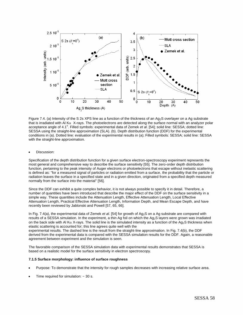
SESSA 58

Figure 7.4. (a) Intensity of the S 2s XPS line as a function of the thickness of an Ag2S overlayer on a Ag substrate

that is irradiated with Al K X-rays. The photoelectrons are detected along the surface normal with an analyzer polar acceptance angle of 4.1

o. Filled symbols: experimental data of Zemek et al. [54]; solid line: SESSA; dotted line:

SESSA using the straight-line approximation (SLA). (b). Depth distribution function (DDF) for the experimental conditions in (a). Dotted line: evaluation of the experimental results in (a); Filled symbols: SESSA; solid line: SESSA with the straight-line approximation.

Discussion: Specification of the depth distribution function for a given surface electron-spectroscopy experiment represents the most general and comprehensive way to describe the surface sensitivity [55]. The zero-order depth distribution function, pertaining to the peak intensity of Auger electrons or photoelectrons that escape without inelastic scattering is defined as: "for a measured signal of particles or radiation emitted from a surface, the probability that the particle or radiation leaves the surface in a specified state and in a given direction, originated from a specified depth measured normally from the surface into the material" [56]. Since the DDF can exhibit a quite complex behavior, it is not always possible to specify it in detail. Therefore, a number of quantities have been introduced that describe the major effect of the DDF on the surface sensitivity in a simple way. These quantities include the Attenuation Length, Effective Attenuation Length, Local Effective Attenuation Length, Practical Effective Attenuation Length, Information Depth, and Mean Escape Depth, and have recently been reviewed by Jablonski and Powell [57, 65, 66]. In Fig. 7.4(a), the experimental data of Zemek et al. [54] for growth of Ag2S on a Ag substrate are compared with

results of a SESSA simulation. In the experiment, a thin Ag foil on which the Ag2S layers were grown was irradiated

on the back side with Al K X-rays. The solid line is the simulated intensity as a function of the Ag2S thickness when elastic scattering is accounted for; this line agrees quite well with the experimental results. The dashed line is the result from the straight-line approximation. In Fig. 7.4(b), the DDF derived from the experimental data is compared with the SESSA simulation results for the DDF. Again, a reasonable agreement between experiment and the simulation is seen. The favorable comparison of the SESSA simulation data with experimental results demonstrates that SESSA is based on a realistic model for the surface sensitivity in electron spectroscopy. 7.1.5 Surface morphology: influence of surface roughness

Purpose: To demonstrate that the intensity for rough samples decreases with increasing relative surface area.

Time required for simulation: ~ 30 s.

SESSA 59

Directory: tutorials\roughness

CLI-files (*.ses): ini.ses, sample.ses, mod.ses


Output-files (output\*.*): rgh

Other files: wu.txt, rgh.txt, cleanup.bat

Procedure: 1. Load the file ini.ses and open the Sample/layer menu (CTRL-1). 2. Load the file mod.ses and watch the ordinate axis of the plot window change when simulations are performed

for different values of the relative surface area, indicating that the total measured intensity drops with increasing surface roughness.

3. Click on the file cleanup.bat thereby deleting unnecessary files in the output directory and creating the file

rgh that may be edited to yield the file rgh.txt. 4. Load compare.g in GNUPlot to view the result (see Fig. 7.5).

Discussion: The comparison in Fig. 7.5 between SESSA simulation results and the experimental data of Wu et al. [58, 59] shows

that the simple model for surface roughness implemented in SESSA provides a rough estimate for the effects of surface roughness on the signal-electron intensity. Note that for a realistically rough surface, the relative surface area

Figure 7.5. Au 4f intensity as a function of the relative surface area. Data points: experimental results from Wu et al. [58, 59]; solid line: results from SESSA.

SESSA 60

assumes values between 1 and 1.2 (see Ref. [5]). Larger values of the relative surface area, such as those measured by Wu et al. for their samples, correspond to porous samples (so called high Brunauer-Emmet-Teller (BET) surfaces [60]).

7.2 Spectral Shape 7.2.1 Au overlayers on a Pb substrate: Spectral shape as a function of overlayer thickness and emission angle

Purpose: Demonstrate the change of spectral shape with emission angle and as a function of the compositional depth profile.

Time required for simulation: ~30 s.

Directory: tutorials\spc

CLI-files (*.ses): ini.ses, mod5.ses, mod25.ses


Output files (output\*.*): *.spc

Other files: cleanup.bat

Procedure: 1. Load the file ini.ses. 2. Load the file mod5.ses that performs a simulation for a 5 Å thick Au overlayer on a Pb substrate for normal

emission and for an emission angle of 60o. Subsequently, load the file mod25.ses that repeats the simulation

for a 25 Å thick overlayer.

Figure 7.6. SESSA simulation results for the Au and Pb 4f, 5p and 5s spectral regions of two samples of Au

overlayers on a Pb substrate and excitation by Al K x-rays. Upper curves: 25 Å Au/Pb; lower curves: 5 Å Au/Pb; Dotted lines: 60

o emission angle; solid lines: emission along the surface normal.

3. Load the file compare.g in gnuplot to view the results as displayed in Fig. 7.6.

SESSA 61

Discussion: The results in Fig. 7.6 clearly show that the shape of the spectrum depends on the compositional depth profile of the sample. The same is seen to be true for the relative intensities of the no-loss peaks. Furthermore, the variation of the spectral shape and the relative intensities with emission angle is different for the two depth profiles considered here. This result is in agreement with the expectation that the combined energy and angular distribution of the signal electron flux emitted from a sample carries information on the chemical composition of a specimen near the surface [13, 53]. 7.2.2 Need for empirical data to realistically describe spectral shapes

Purpose: To show that incorporation of empirical data in SESSA provides a convenient tool for quantitative simulation not only of spectral intensities but also of spectral shapes.


Directory: tutorials\aes-empirical

CLI-files (*.ses): cu.ses, cu-emp.ses


Output-files (output\*.*):

Procedure:

1. Load the file cu.ses and open the Model calculation menu (CTRL-7). The Al K Cu XPS spectrum is seen in this menu. Note that the LMM Auger part that is located in the range of kinetic energies between 700 eV and 1000 eV does not look very realistic. Go to the "Sample/peak" menu (CTRL-2) and click on any of the Auger peaks in the peak selection list. The graphical display of the intrinsic peak shape shows that the standard functional forms (Gaussian, Lorentzian, Doniach- Sunjic) do not resemble a realistic Auger peak (see Fig. 7.7).

2. Load the file cu-emp.ses and open the "Model calculation" menu (CTRL-7). Open the Sample/peak menu

(CTRL-2) to see that all Auger peaks except one were removed. The remaining empirical Auger peak comprises a broad spectral range. In the Model calculation menu graphical display, a spectrum similar to the previous one is shown, but the Auger part now looks much more realistic, as shown in Fig. 7.7.

Discussion: A drastic difference is seen between the two spectra created by the above procedure (Fig. 7.7). However, comparison of the partial intensities of the Cu LMM peaks reveals that the spectral shape of the signal-electron sources is the only difference; the partial intensities are identical! To appreciate this, note that a simulation of a spectrum in SESSA proceeds in two steps: first, the partial intensities are calculated for a given sample, experimental conditions, etc. The partial intensities represent the number of electrons emitted from a given atomic subshell in a given atom that eventually reach the detector after experiencing a certain number of inelastic collisions. The parameters in the SESSA databases for this purpose are believed to be realistic. In the next step, the partial energy distributions are derived from the energy distribution at the source and the probability for an energy loss in an individual excitation (that is the differential inelastic inverse mean free path, DIIMFP). Although realistic data for the DIIMFP are available within SESSA for a limited number of materials for which detailed optical measurements are found in the literature, realistic data for the spectral shape of an Auger-electron transition and photoelectron transition are not presently part of the SESSA databases. This situation is particularly problematic for Auger-electron transitions, and emphasizes the necessity for empirical data when simulating the spectral shape.

SESSA 62

Figure 7.7. XPS spectrum of a Cu sample excited by Al K x-rays. Upper curve: simulation result from SESSA using empirical data for the Cu LMM Auger transition; lower curve: the same simulation based on the default peak shapes contained in SESSA. 7.2.3 Transfer of spectral data between different spectrometers

Purpose: Demonstrate that intercomparison of spectra acquired on different instruments can be significantly facilitated when a flexible simulation tool is available that accounts for instrumental effects. In the present case, an effect of solid angle is studied.


Directory: tutorials\transfer

CLI-files (*.ses): ini.ses


Output-files (output\*.*): reg1.spc

Procedure: Load the file ini.ses and open the Model calculation menu (CTRL-7). The graphical display in this menu is essentially the same as the results shown in Fig. 7.8.

Discussion: The results in Fig. 7.8 show that complex differences in spectral shapes can occur for instruments that differ in certain properties. In the present example, this concerns the solid angle of acceptance of the analyzer. This makes it very difficult to compare quantitative information on published spectra from different types of instruments. A simulation such as SESSA can help avoid such problems if instrumental effects on the spectral shape are realistically simulated.

SESSA 63

Figure 7.8. XPS spectra of a 2 Å thick Ni layer on a Cu substrate excited by Al K x-rays. Dotted line: simulation results from SESSA assuming a hemispherical analyzer (HMA) for energy selection; solid line: SESSA simulation using a cylindrical mirror analyzer (CMA). To facilitate comparison, the two curves have been slightly shifted in energy relative to each other. 7.2.4 Handbook of simulated XPS spectra

Purpose: Using the extensive databases in SESSA and the flexibility offered by the CLI, it is possible to produce large customized reference data sets.

Time required for simulation: several minutes.

Directory: tutorials\handbook

CLI-files (*.ses): ini.ses, handbook.ses, handbook-brief.ses, dosim.ses

Output-files (output\*.*): XPS spectra of elemental solids throughout the periodic system, with and without a 5 Å thick carbon contamination layer.

Procedure: 1. Load the file ini.ses. 2. Load the file handbook_brief.ses to get a quicker impression of what handbook.ses does when you start

it. 3. Edit the file dosim.ses and uncomment the indicated line. 4. Run the file handbook_brief.ses again, now producing a handbook of XPS spectra recorded on samples

with a 5 Å carbon contamination layer.

SESSA 64

Discussion: The above CLI files produce two extensive reference data sets for a collection of elemental solids throughout the periodic table. In the second run, a systematic change in the experimental conditions is simulated by adding a 5 Å thick carbon-contamination layer to each sample.

7.3 Techniques other than conventional AES/XPS 7.3.1 Total Reflection XPS (TRXPS)

Purpose: Illustrate the fact that the surface sensitivity is generally determined by both the excitation depth distribution as well as the emission depth distribution function.


Directory: tutorials\trxps

CLI-files (*.ses): sample.ses, xps_sim.ses, trxps_sim.ses, trxps..ses

GNUPLOT-files (*.g) :

Output-files (output\*.*): xpsreg1.spc, trxpsreg1.spc

Procedure: 1. Open the Sample window in the GUI and press CTRL-l to load the session file sample.ses. After a while, the

structure of the sample is updated on the screen and is seen to consist of a very thin C- contamination layer (layer 1, 0.5 Å) on top of 8 Å of SiO2 on an Si substrate (see Fig. 7.9). The upper 24 layers are seen to consist of a contribution labeled [trxps] and a normal unlabeled contribution. The concentration of the species labeled [trxps] decreases exponentially with depth. In the Sample/Peak menu, it can also be seen that each peak appears in duplicate, unlabeled as well as labeled. These settings were chosen to mimic a total-reflection XPS experiment, where the incidence angle of the exciting x-radiation is chosen close to the critical angle for total reflection, leading to a dramatic decrease of the characteristic length (or depth) for creation of photoelectrons. In the present example, this characteristic length was arbitrarily chosen to be 20 Å, a typical value in TRXPS.

2. Next, load the file xps_sim.ses. This file performs a simulation for all peaks (labeled as well as unlabeled), and

writes the corresponding output into the directory output. Since the labeled and unlabeled peaks have the same peak shape and energy, they are added in the resulting spectrum output\xpsreg1.spc. Thus the simulated spectrum should resemble a conventional XPS spectrum, as indeed it does (see Fig. 7.10(a)).

3. When the file trxps_sim.ses is loaded next, the same simulation is repeated but the unlabeled peaks are

deleted from the spectra prior to the simulation. In consequence, the resulting spectrum output\trxpsreg1.spc now corresponds to a depth distribution of excitation for the species labeled [trxps] only. The result is displayed in Fig. 7.10(b). The inelastic background is seen to be significantly decreased, indicating that the surface sensitivity of this spectrum is higher than for a conventional XPS measurement.

4. It should be noted here that, in these simulations, the incidence direction of the x-rays was chosen along the

surface normal, as was the detection direction. In other words, the change in the surface sensitivity due to the grazing incidence of the x-rays was simulated only by taking into account the depth distribution of the excitation. For a more realistic simulation of TRXPS with the present version of SESSA, it is imperative to properly account for the experimental geometry since the relative peak intensities for photoelectrons with different asymmetry parameters depend sensitively on the values of this parameter, in particular for typical TRXPS geometrical configurations. It is easy to perform realistic simulations with SESSA; one merely has to specify the correct geometrical configuration in the Geometry menu. Since the example studied here merely serves illustrative purposes and is not compared with actual experimental data, the simulations were performed for the default geometrical configuration.

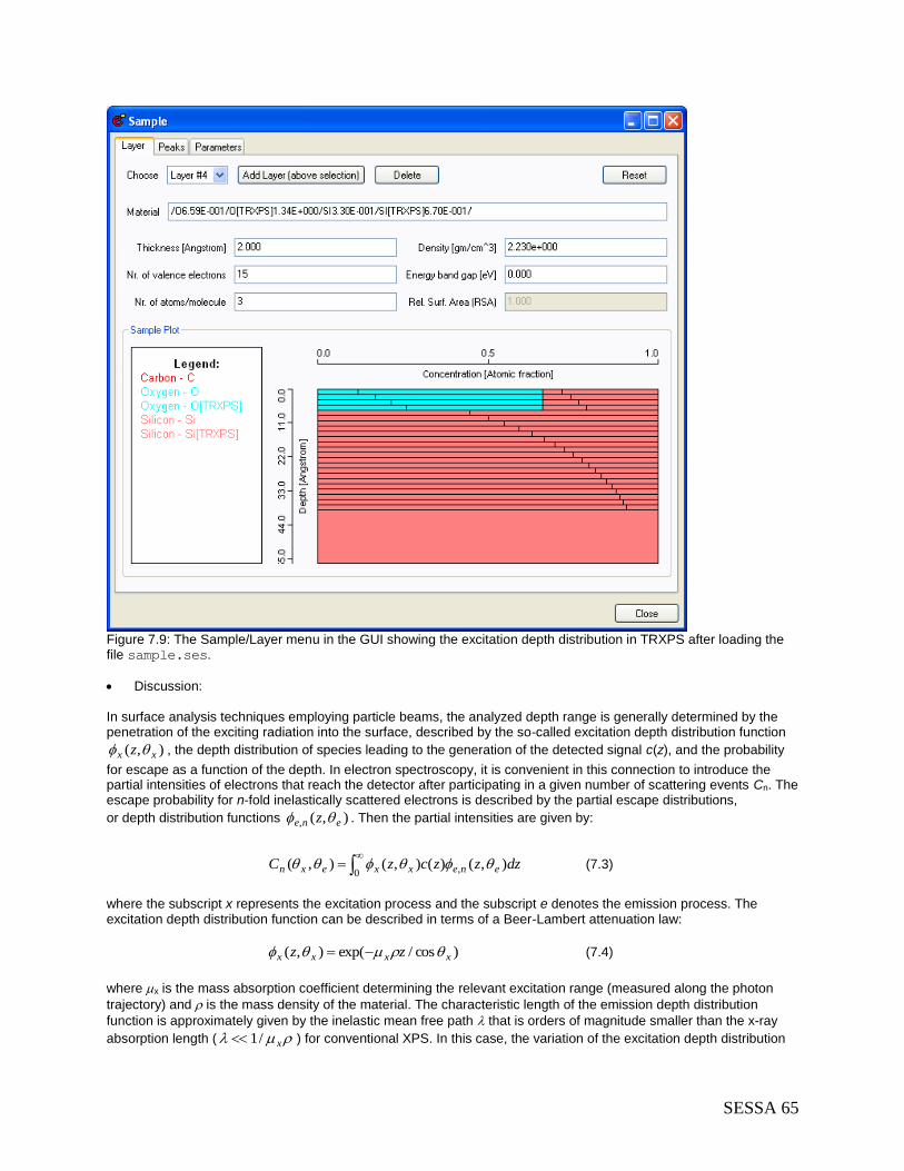
SESSA 65

Figure 7.9: The Sample/Layer menu in the GUI showing the excitation depth distribution in TRXPS after loading the file sample.ses.

Discussion: In surface analysis techniques employing particle beams, the analyzed depth range is generally determined by the penetration of the exciting radiation into the surface, described by the so-called excitation depth distribution function

),( xx z , the depth distribution of species leading to the generation of the detected signal c(z), and the probability

for escape as a function of the depth. In electron spectroscopy, it is convenient in this connection to introduce the partial intensities of electrons that reach the detector after participating in a given number of scattering events Cn. The escape probability for n-fold inelastically scattered electrons is described by the partial escape distributions,

or depth distribution functions ),(, ene z . Then the partial intensities are given by:

dzzzczC enexxexn ),()(),(),( ,0

(7.3)

where the subscript x represents the excitation process and the subscript e denotes the emission process. The excitation depth distribution function can be described in terms of a Beer-Lambert attenuation law:

)cos/exp(),( xxxx zz (7.4)

where x is the mass absorption coefficient determining the relevant excitation range (measured along the photon

trajectory) and is the mass density of the material. The characteristic length of the emission depth distribution

function is approximately given by the inelastic mean free path that is orders of magnitude smaller than the x-ray

absorption length ( x/1 ) for conventional XPS. In this case, the variation of the excitation depth distribution

SESSA 66

Figure 7.10. Simulated spectra of a sample consisting of a 0.5 Å thick C-contamination layer on top of a 8 Å thick SiO2 layer on a Si substrate. (a) Simulation of a conventional XPS spectrum; (b) total reflection XPS spectrum, where the angle of incidence of the x-rays is close to the angle for total reflection. with depth in the integral (7.3) can be neglected and the surface sensitivity of XPS is entirely determined by the escape process.

SESSA 67

When the angle of incidence of the x-rays is close to the critical angle for total reflection cx, , the characteristic length

for the excitation process becomes comparable to the inelastic mean free path [61], and an angular variation of the (glancing) incidence angle according to Eq.(7.3) allows probing of different depth regions by effectively changing the excitation depth distribution experimentally. In this case, the detected photoelectrons mainly escape from shallow depths (as indicated by the depth distribution of the species labeled [trxps] in the Sample/Layer menu), and consequently the higher order partial intensities that make up the inelastic background are suppressed since the emission depth distribution function for increasing order of

scattering samples increasingly larger depths (approximately ein cos/ for n-th order scattering [13]). This explains

the reduced inelastic background seen in the TRXPS spectrum in Fig. 7.10(b).

7.3.2 Ion-induced Auger-electron emission

Purpose: Demonstrate that the source depth distribution can be specified in a flexible way using a technique involving chemical-state labeling.

Time required for simulation: ~35 min.

Directory: tutorials\ion-induced

CLI-files (*.ses): sim.ses, geo.ses, cu.ses

GNUPLOT-files (*.g): pi.g,spc.g

Output-files (output\*.*): cucuLM9_emitting.*

Other files: CULMM.REG

Procedure: Start SESSA. 1. Open the sample menu (CTRL-5). Load the file cu.ses and wait a moment. The commands in this file set up a

depth profile of emitters distributed with a Gaussian profile at 12 Å mean depth and a full width at half maximum intensity of 5 Å. This profile is assumed to be caused by energy deposited in the solid by some kind of incident particle (e.g., ions) and the energy deposition profile is assumed to be related to the depth profile of Auger electron emission. The profile is seen in the sample menu after SESSA has processed the commands in this file. By clicking on the various layers in the depth profile and observing the material box in the sample GUI menu, it is seen how the chemical state labeling can be used to specify a depth profile of emitters in a flexible way.

2. Load the file geo.ses. This sets up the geometry: the analyzer is rotated around the sample surface normal in

the range between 0o and 60

o.

3. Load the file sim.ses. SESSA performs a simulation of the spectrum for the specified geometries. Open the

simulation menu (CTRL-7) before or after loading sim.ses to see the simulation results. 4. Open the Sample/Peak menu and choose "partial intensities" in the display selection box to view the partial

intensities. You may wish to double click on this window to transfer its contents to the separate plot window that can be enlarged to fit the screen, improving clarity.

Discussion: Figure 7.11 shows the result of the simulation. It is seen that both the peak height and shape depend on emission angle. Inspection of the partial intensities reveals the reason for the dependence of the peak shape on the emission angle: for more oblique emission, the signal electrons have to travel a longer distance through the solid, thereby increasing the probability for an energy loss. In principle, measurements of the angular distribution of the peak shape contain information on the emission depth distribution function (EDDF). However, it is difficult to rigorously retrieve EDDFs from such measurements. Simulations that optimize the consistency between experiment and theory by varying the depth distribution of the emitters provide a straightforward means of obtaining at least a rough impression of the EDDF.

SESSA 68

Figure 7.11. Cu LMM Auger spectra for different emission angles and for the source depth distribution shown in the inset. These results simulate ion-induced Auger electron spectra.

8 CALLING SESSA FROM AN EXTERNAL APPLICATION

A special and important feature of SESSA is that it can not only be operated interactively as a stand-alone program, but that it can also be run from within an external application. This external application could be a simple program, written by a SESSA user in which a certain parameter such as the thickness of a given layer in a specimen is varied over a certain range in order to compare measured and simulated spectra as a function of layer thickness. The external software could also be more complex software such as a non-linear least-squares fitting program that automatically optimizes the structural parameters of a specimen so that the final result of a series of SESSA simulations optimally matches experimental data. That is, a user could retrieve the optimal specimen structure by means of an inverse modeling approach in which SESSA provides the simulation core. An external application can thus harness the full potential of SESSA, for an arbitrary application, in a simple way, as explained below. This feature of SESSA was introduced in Version 1.3. The communication of an external program with the SESSA software is implemented via the so-called piping mechanism. This method implies that the external software actually invokes the SESSA software and subsequently passes commands to SESSA by writing a string of characters to a file-handle that was opened for this purpose. In addition, feedback from SESSA can be read from the same filehandle. This mechanism is what is generally referred to as “piping”. The commands that are passed to SESSA via the piping mechanism are identical to the SESSA CLI-commands that are explained in this Users’ Guide. For the external software to access results of SESSA simulations or database operations, one needs to tell SESSA to write the corresponding information to a file, open the corresponding file, and read the relevant information from within the external software. This procedure is explained in the sample programs SESSA_LINUX.c in Table 8.1 (for the Linux or MacIntosh OSX operating system) and SESSA_WINDOWS.c in Table 8.2 (for the Windows operating system). These programs are also included in digital form with the SESSA software in the folder “External software”. These sample programs are intended to guide a user in applying this special feature of SESSA. They can also be used as a first building block to incorporate the functionality of SESSA in any software for quantification of electron spectra. Note that the names of files and directories that are used in these sample programs will need to be changed according to the user’s installation of SESSA in order for these programs to run.

SESSA 69

While the mechanism of calling SESSA from an external application, as explained above, is completely analogous on the Windows and Linux or MacIntosh OSX operating systems, it is simpler on the latter and therefore the various required steps in the file SESSA_LINUX.c in Table 8.1 will be described first.

8.1 The Program SESSA_LINUX.c In the section “//1.)”, the usual include statements and variable declarations for the sample program are given. The filepointer named fp is declared to serve as the pipe through which commands are relayed to SESSA. In the section “//2.)”, the pipe is opened, i.e., the SESSA software is invoked and each string of characters written to the filepointer fp at any later time via a call to fprintf(fp, “SESSA CLI-command” will be interpreted by SESSA as if a command had been interactively made on the SESSA CLI console. Note that the first argument of the popen command should contain the full directory path and filename of the SESSA executable as it is installed on the user’s computer. The option ”-c” must be added to indicate that SESSA is to be run in the console mode. A user may verify the correct value of the path and filename by opening a shell in Linux or MacIntosh OSX, and typing the path and filename of the SESSA-executable with the “-c” option appended, and SESSA should start and run in the console mode and will accept the CLI commands issued by the user in the shell.

Commands for the control of SESSA can be written as appropriate strings of characters to the filepointer fp using the fprintf statement as exemplified in section “//3.)”. These commands are issued within the external program and passed to SESSA after the popen statement of section “//2.)”. Note that the buffer of the filepointer needs to be flushed using a fflush(fp) statement after each SESSA CLI command in order for the command to be actually processed. In the sample program, SESSA is reset to its default conditions by the first command, the material is then set to SiO2, the number of collisions in the simulation is set to 10, and the simulation is performed by the following command. The subsequent three commands make SESSA write the desired output to a file, which is then opened for further processing in section “//4.)”. The last CLI command deactivates SESSA. In section “//4.)”, one of the files produced by the software, as discussed above, is opened and the partial intensities of the Si 2p peak are read by the external software. In the simple example program, these partial intensities are finally written to the screen, thereby demonstrating the means of bidirectional communication between SESSA and the external application.

8.2 The Program SESSA_WINDOWS.c The mechanism for external calling of SESSA with the Windows operating system is analogous to that described in the previous section. The only essential difference is that SESSA needs to be invoked from the command line within Windows before the external application is launched. After issuing one of the following the commands on a Windows

terminal console: >SESSA -p

or >SESSA –c

SESSA starts in the pipemode. SESSA then runs in the background without opening windows for the graphical user interface or any other action noticeable by the user. In this mode, SESSA has opened a so-called named pipe identified by “\\.\pipe\SessaPipe” through which it expects valid SESSA CLI commands at a later time. In the sample program SESSA_WINDOWS.c in Table 8.2, the section marked “//1.)” provides the include statements and variable declarations used within the sample program. In the sections “//F1.)” and “//F2.)”, the functions WriteToPipe and WaitForCommand are declared that are used to relay commands and flush the buffer. These functions are equivalent to the fprintf and fflush commands shown in section “//3.)” of Table 8.1.

The filepointer named hFile is declared in section “//2)” with the CreateFile command as the pipe through which desired CLI commands are relayed to SESSA from the external program. This is done by opening a channel to the named pipe “\\.\pipe\SessaPipe” that was established previously when SESSA was started with the “-p” or “-c” option. All further communications from the external program to SESSA can then proceed by writing a string of characters corresponding to one or more valid SESSA CLI commands to this named pipe. The communications in the opposite direction, i.e., from SESSA to the external program, again proceed via the output files produced by SESSA, as in the case described in the previous section.

SESSA 70

Table 8.1. Illustrative program for calling SESSA from an external application using the Linux or the MacIntosh OSX operating system.

//Calling SESSA from an external application on LINUX or the MacIntosh OSX operating system //1.) Variable declarations #include <stdio.h> #include <stdlib.h> #include <math.h> main() { double x,y; int k; char c[100]; FILE *fp; //2.) activate SESSA if (( fp=popen("/Applications/SESSA\\ v1.3.app/Contents/MacOS/SESSA\\ v1.3 -c","w")) == NULL) { perror("popen");exit(1); } //3.) Now pipe commands to SESSA just as you would in the SESSA CLI fprintf(fp, "PROJECT RESET\n"); fflush(fp); fprintf(fp, "SAMPLE SET MATERIAL /Si/O2/ LAYER 1\n"); fflush(fp); fprintf(fp, "MODEL SET NCOL 10 REGION 1\n"); fflush(fp); fprintf(fp, "MODEL SIMULATE\n"); fflush(fp); fprintf(fp, "PROJECT SAVE OUTPUT \"/Users/werner/Desktop/testsessalinux/output/test\"\n"); fflush(fp); fprintf(fp, "SAMPLE PEAK PLOT PART_INT PEAK 1\n"); fflush(fp); fprintf(fp, "PLOT SAVE DATA \"/Users/werner/Desktop/testsessalinux/output/Si2p.cn\"\n"); fflush(fp); fprintf(fp, "quit\n"); fflush(fp); pclose(fp); //4.) Now we can open the output SESSA has produced for further analysis fp=fopen("/Users/werner/Desktop/testsessalinux/output/Si2p.cn","r"); if(fp==NULL) { printf("Error:can’t open file.\n");} else { k=0; printf("First partial intensities:\n"); while(fgets(c,100,fp)!=NULL) { if (c[0]=='#') continue; fscanf(fp, "%le %le",&x,&y ); if (k>1) {printf("%le %le\n",x,y);} k++; } }

}

In section “//3.)”, CLI commands are sent to SESSA for processing through the named pipe using the WriteToPipe function in conjunction with the WaitForCommand function that clears the buffer. As in the example program of Table 8.1, a simulation is setup and run for SiO2 and, in the present case, the partial intensities for the Si 2s peak are written to a file which is then read in section “//4.)”. These partial intensities are again printed on the screen, thereby demonstrating the mechanism for bidirectional communication between SESSA and the external program.

SESSA 71

Table 8.2 Illustrative program for calling SESSA from an external application using the Windows operating system.

//SESSA_WINDOWS.c /Calling SESSA on the Windows operating system //1.) Variable Declarations #include <windows.h> #include <stdio.h> #define BUFSIZE 1024 HANDLE hFile; char buffer[BUFSIZE]; //F1.) Function to actually relay a command to SESSA void WriteToPipe(char* message) { DWORD dwWrite; BOOL success; printf("Sending message %s to pipe\n", message); strcpy(buffer, message); strcat(buffer, "\n"); success = WriteFile(hFile, buffer, strlen(buffer), &dwWrite, NULL); if(!success) { printf("WriteFile to pipe failed (%s, GLE=%d)\n", message, GetLastError() ); exit(-1); } } //F2.) Clear Buffer and wait void WaitForCommand() { BOOL success, finished; DWORD cbRead; do { success = ReadFile(hFile, // pipe handle buffer, // buffer to receive reply BUFSIZE, // size of buffer &cbRead, // number of bytes read NULL); // not overlapped if(!success && GetLastError()!=ERROR_MORE_DATA) break; buffer[cbRead] = '\0'; printf("Sessa: %s", buffer); finished = strstr(buffer, "Done")!=NULL; } while(!success || !finished);// repeat loop if ERROR_MORE_DATA } int main() { FILE* fp; //2.) Open the pipe to SESSA hFile = CreateFile("\\\\.\\pipe\\SessaPipe", GENERIC_WRITE | GENERIC_READ, 0, NULL, OPEN_EXISTING, 0, NULL); if(hFile == INVALID_HANDLE_VALUE) { printf("CreateFile failed for Named Pipe client\n" ); exit(-1);} //3.) Pass CLI commands to SESSA WriteToPipe("PROJECT RESET"); WaitForCommand(); WriteToPipe("SAMPLE SET MATERIAL /Si/O2/ LAYER 1"); WaitForCommand(); WriteToPipe("MODEL SIMULATE");

SESSA 72

WaitForCommand(); WriteToPipe("SAMPLE PEAK PLOT PART_INT PEAK 1"); WaitForCommand(); WriteToPipe("PLOT SAVE DATA \"C:\\Temp\\Si2s.txt\""); WaitForCommand(); WriteToPipe("QUIT"); WaitForCommand(); CloseHandle(hFile); //4.) Open the SESSA output for further analysis fp = fopen("C:\\Temp\\Si2s.txt", "r"); if(fp==NULL) { puts("Error: cannot open data file."); exit(-1); } else { puts("Showing partial intensities for the Si2s peak"); puts("n\t\tC_n"); while(fgets(buffer, BUFSIZE, fp)!=NULL) { double x, y; if(buffer[0]=='#') continue; fscanf(fp, "%le %le", &x, &y ); printf("%le\t%le\n", x, y); } fclose(fp); } }

SESSA 73

9 GETTING HELP, TESTING AND DEBUGGING

9.1 Getting Help Online help is provided by SESSA in the GUI and in the CLI. In the GUI, selecting Help in the main menu and then selecting SESSA help and then Read Manual invokes Adobe Acrobat Reader or other software to display a PDF file. Most of the text from this Users' Guide present will then be displayed on the screen, together with bookmarks and thumbnails that facilitate navigation through this documentation. In the CLI, typing HELP in any scope produces corresponding help messages. This can also be achieved by opening the command syntax tree in the CLI console by clicking on the button Command List and clicking on the command in the list for which information is desired. Further information on SESSA and its applications can be found by accessing the SESSA home page. This can be done by selecting Visit Homepage from the Help menu.

9.2 SESSA User Forum The SESSA User Forum is accessed by choosing "Visit forum" from the Help menu. This Forum exists to promote exchange of information and to help address questions among SESSA users.

9.3 General Information The Help menu also gives access to the About and the Disclaimer boxes. The disclaimer box displays the message that can also be found on page ii of this Users’ Guide. The About box provides some general information on the history of SESSA and acknowledges software resources that were helpful in its development. The latter comprise:

NetCDF: http://www.unidata.ucar.edu/packages/netcdf/

wxWindows: http://www.wxwindows.org/

CVS: http://www.cvs.org/

Inno Setup: http://www.jrsoftware.org/isinfo.php

SCITE: http://www.scintilla.org/SciTE.html

Free Borland C++ 5.5 Compiler: http://www.borland.com/

GNUPlot: http://www.gnuplot.info The authors gratefully acknowledge the use of these resources for the development of SESSA [63].

9.4 Testing and Debugging

Despite the complexity of the software, SESSA was developed by a very small team (see the About box). For successful testing of the software, it was considered essential to involve a larger group of users. A world-wide-web interface has been set up for the exchange of information on SESSA (see Section 8.2) as well as to facilitate the reporting of bugs described here. From the Help menu, choose the Submit Bug option and then clicking on "Open new task anonymously" from the SESSA-bugfix webpage and following the instructions there. It is essential to add the files "debug_crash.ses" and "debug_last.ses" at this stage. If, after inspecting the list for the given class and subsystem, a user concludes that a particular error is not present in this list, the option I found a NEW feature/bug in the Databases subsystem of SESSA should be selected at the top of the page to report a bug not previously listed. The local email program will pop up with an appropriate address. A brief explanation of the observed bug should be given in the body of the message. Furthermore, the following message will appear in the body of the message: "Please attach debug.ses/debug_crash.ses/debug_last.ses (location: SESSA binaries)". This message prompts a user to attach any of these files that are present when submitting the bug report. During a SESSA session, a file debug.ses is written that contains all commands issued. If the program terminates

properly, this file is renamed to debug_last.ses. If the program crashes, the file debug.ses contains all

commands necessary to analyze the problem at hand. If SESSA is run again after the crash, this file is renamed to debug_crash.ses. To facilitate analysis of the reported bug, it is essential that the tester attach any of the above files that are present in the directory where the SESSA binaries reside. To ensure that these files are up to date, a bug should always be reported as soon as possible after it was encountered. If the program crashes it should be started again and a bug report should immediately be sent. If the program is still active, the Submit bug option in the Help menu should be chosen and the bug should be reported accordingly.

http://www.unidata.ucar.edu/packages/netcdf/

http://www.wxwindows.org/

http://www.cvs.org/

http://www.jrsoftware.org/isinfo.php

http://www.scintilla.org/SciTE.html

http://www.borland.com/

http://www.gnuplot.info/

SESSA 74

10 CONTACTS If you have comments or questions about the database, the NIST Measurement Services Division Standard Reference Data Program would like to hear from you. Also, if you have any problems with the disk or installation, please let us know by contacting: National Institute of Standards and Technology 100 Bureau Drive, Stop 2320 Gaithersburg. MD 20899-2320 E-mail: [email protected] Phone: (301) 975-2008 FAX: (301) 926-0416 If you have technical questions relating to the database, contact: Dr. C.J. Powell National Institute of Standards and Technology 100 Bureau Drive, Stop 8370 Gaithersburg. MD 20899-8370 E-mail: [email protected] Phone: (301) 975-2534 FAX: (301) 216-1134 Prof. Dr. W.S.M. Werner Institut fűr Allgemeine Physik Vienna University of Technology Wiedner Hauptstr. 8-10 A-1040, Vienna, Austria E-mail: [email protected] Phone: +43-1-58801-13462 FAX: +43-1-58801-13499 Dr. W. Smekal Institut fűr Allgemeine Physik Vienna University of Technology Wiedner Hauptstr. 8-10 A-1040, Vienna, Austria E-mail: [email protected] Phone: +43-1-58801-13463 FAX: +43-1-58801-13499

11 ACKNOWLEDGMENTS The authors are grateful for the work of Herbert Beilschmidt, Thomas Cabela, Gerald Richter, Ljubomir Milanovic, Fabian Moser, Alexander Gross, Gunther Cronenberg, Stephan Heiss, Lukas Hille, Rudolf Höfler, Wernfried Mayr-Schmölzer, Heinrich Schindler, and Thomas Hisch in programming and database compilation at the Institute of Applied Physics, Vienna University of Technology.

SESSA 75

Bibliography [1] W. S. M. Werner, Surf. Interface Anal. 31, 141 (2001). [2] K. D. Sevier. Low Energy Electron Spectrometry. Wiley-Interscience, New York, 1972. [3] T. A. Carlson, Photoelectron and Auger Spectroscopy, Plenum, New York, 1975. [4] W. A. Coghlan and R. E. Clausing, Atomic Data 5, 317 (1973). [5] W. S. M. Werner, Surf. Interface Anal. 23, 696 (1995). [6] S. Tanuma, C. J. Powell, and D. R. Penn, Surf. Interface Anal. 21, 165 (1994). [7] S. Tougaard, Surf. Interface Anal. 25, 137 (1997). [8] W. H. Gries and W. S. M. Werner, Surf. Interface Anal. 16, 149 (1990).

[9] N. F. Mott and H. S. W. Massey. The Theory of Atomic Collisions, Oxford University Press, Oxford, 1949. [10] H. S. W. Massey and E. H. S. Burhop, Electronic and Ionic Impact Phenomena, Clarendon Press, Oxford, 1952. [11] I. S. Tilinin and W. S. M. Werner, Phys. Rev. B 46, 13739 (1992). [12] W. S. M. Werner, Phys. Rev. B 55,14925 (1997). [13] W. S. M. Werner, Surf. Interface Anal. 23, 737 (1995). [14] W. S. M. Werner, Phys. Rev. B 52, 2964 (1995). [15] W. S. M. Werner, Surf. Science 526, L159 (2003). [16] W. S. M. Werner, in Surface Analysis by Auger and X-Ray Photoelectron Spectroscopy, D. Briggs and J. T.

Grant, editors, IM Publications, Chichester, 2003, p. 235. [17] W. S. M. Werner and P. Schattschneider, J. Electron Spectrosc. Relat. Phenom. 143, 81 (2005). [18] R. Shimizu and Z.-J. Ding, Rep. Prog. Phys. 55, 487 (1992). [19] L. D. Landau. J. Phys. (Moscow) 8, 201 (1944).

[20] K. M. Case and P. F. Zweifel, Linear Transport Theory, Addison-Wesley, Reading,1967. [21] D. R. Penn, Phys. Rev. B 35, 482 (1987).

[22] C. J. Powell (private communication). [23] R. C. Weast and M. J. Astle, CRC Handbook of Chemistry and Physics, 60

th ed., CRC Press, Boca Raton, 1980.

[24] F. J. Garcia de Abajo, Rev. Mod. Phys. 82, 209 (2010).

[25] E. D. Palik, Handbook of Optical Constants of Solids, Academic Press, New York, 1985. [26] E. D. Palik, Handbook of Optical Constants of Solids II, Academic Press, New York, 1991. [27] B. L. Henke, E. M. Gullikson, and J. C. Davis, At. Data Nucl. Data Tables 54, 181 (1993). [28] S. Tanuma, C. J. Powell, and D. R. Penn, Surf. Interface Anal. 43, 689 (2011). [29] J. Vinson, J. J. Rehr, J. J. Kas, and E. L. Shirley, Phys. Rev. B 83, 115106 (2011). [30] A. P. Sorini, J. J. Kas, J. J. Rehr, M. P. Prange, and Z. H. Levine, Phys. Rev. B 74, 165111 (2006). [31] A. Frydman, D. G. Castner, M. Schmal, and C. T. Campbell, J. Catalysis 157, 133 (1995). [32] A. C. Yates, Comp. Phys. Comm. 2, 175 (1971). [33] R. A. Bonham and T. G. Strand, J. Chem. Phys. 39, 2200 (1963).

[34] A. Jablonski, F. Salvat, and C J Powell, NIST Electron Elastic-Scattering Cross-Section Database (SRD 64), Version 3.2 (National Institute of Standards and Technology, Gaithersburg, 2010); http://www.nist.gov/srd/nist64.cfm.

[35] I. S. Tilinin, Sov. Phys. JETP 67, 1570 (1988). [36] J. H. Scofield, J. Electron Spectrosc. Relat. Phenom. 1, 129 (1976). [37] J. J. Yeh and I. Lindau, At. Data Nucl. Data Tables 32, 1 (1985). [38] M. B. Trzhaskoskaya, V. I. Nefedov, and V. G. Yarzhemsky, At. Data Nucl. Data Tables 77, 97 (2001). [39] M. B. Trzhaskoskaya, V. I. Nefedov, and V. G. Yarzhemsky, At.. Data Nucl. Data Tables 82, 257 (2002). [40] R. F. Reilman, A. Msezane, and S. T. Manson, J. Electron Spectrosc. Relat. Phenom. 8, 289 (1976). [41] E. Casnati, A. Tartari, and C. Baraldi, J. Phys. B: At. Mol. Phys. 15, 155 (1982). [42] M. Gryzinski, Phys. Rev. 138, A336 (1965). [43] C. R. Worthington and S. G. Tomlin, Proc. Phys. Soc. London A 69, 401 (1956). [44] G. P. Williams, X-ray Data Booklet, Lawrence Berkeley National Laboratory, University of California, Berkeley,

2001. [45] J. H. Hubbell, P. N. Trehan, N. Singh, B. Chand, D. Mehta, M. L. Garg, R. R. Garg, S. Singh, and S. Puri, J.

Phys. Chem. Ref. Data, 23, 339 (1994); ibid. 33, 621 (2004). [46] W. Bambynek, in Proceedings of International Conference on X-ray and Inner Shell Processes, Leipzig,

Germany, 1984. [47] E. H. S. Burhop, J. Phys. Radium 16, 625 (1955). [48] R. Shimizu, Japan. J. Appl. Phys. 22, 1631 (1983). [49] S. Chandrasekhar, Radiative Transfer, Dover Publications, New York, 1960. [50] W. S. M. Werner, I. S. Tilinin, and A Jablonski, Surf. Interface Anal. 23, 823 (1995). [51] O. A .Baschenko, G. V. Machavariani, and V. I. Nefedov, J. Electron Spectrosc. Relat. Phenom. 34, 305 (1984). [52] M. P. Seah and R. White, Surf. Interface Anal. 33, 960 (2002). [53] P. J. Cumpson, J. Electron Spectrosc. Relat. Phenom. 73, 25 (1995). [54] J. Zemek, P. Jiricek, S. Hucek, A. Jablonski, and B. Lesiak, Surf. Science 473, 8 (2001).

http://www.nist.gov/srd/nist64.cfm

SESSA 76

[55] W. S. M. Werner, W. H. Gries, and H. Störi, J. Vac. Sci. Technol. A 9, 21 (1991).

[56] ISO 18115-1:2010, Surface chemical analysis – Vocabulary – Part 1: General terms and terms used in spectroscopy (International Organization for Standardization, Geneva); https://www.iso.org/obp/ui/#iso:std:iso:18115:-1:ed-1:v1:en.

[57] C. J. Powell and A. Jablonski, Surf. Interface Anal. 33, 211 (2002). [58] O. K. T. Wu and E. M. Butler, J. Vac. Sci. Technol. 30, 453 (1982). [59] O. K. T. Wu, G. G. Peterson, W. J. La Rocca, and E. M. Butler, Appl. Surf. Science 11/12, 118 (1982). [60] S. Brunauer, P. H. Emmet, and E. Teller, J. Am. Chem. Soc. 60, 309 (1938). [61] B. L. Henke, Phys. Rev. A 6, 94 (1972). [62] A. Jablonski, F. Salvat, and C. J. Powell, J. Phys. Chem. Ref. Data 33, 409 (2004).

[63] A vendor is identified to specify the source of experimental data, information or software. Such identification does not imply recommendation or endorsement by the National Institute of Standards and Technology, not does it imply that the data concerned are the best available for the purpose.

[64] A commercial product is identified to specify conditions for an experimental test. Such identification does not imply recommendation or endorsement by the National Institute of Standards and Technology, not does it imply that the product concerned is the best available for the purpose.

[65] A .Jablonski and C. J. Powell, Surf. Science Reports 47, 33 (2002). [66] A. Jablonski and C. J. Powell, J. Vac. Sci. Tech. A 21, 274 (2003). [67] A. Jablonski, F. Salvat, and C. J. Powell, Comput. Phys. Commun. 165, 157 (2005).

[68] A. V. Naumkin, A. Kraut-Vass, and C. J. Powell, NIST X-ray Photoelectron Spectroscopy Database, SRD 20, Version 4.1 (National Institute of Standards and Technology, Gaithersburg, 2012); http://www.nist.gov/srd/nistweb20v4.htm.

[69] M. B. Trzhaskoskaya, V. I. Nefedov, and V. G. Yarzhemsky, At. Data Nucl. Data Tables 77, 97 (2001). [70] P. S. Shaw, U. Arp, and S. H. Southworth, Phys. Rev. A 54, 1463 (1996). [71] J. W. Cooper, Phys. Rev. A 47, 1841 (1993). [72] D. R. Baer and M. H. Engelhard, J. Electron Spectrosc. Relat. Phenom. 178/179, 415 (2010). [73] H. P. C. E. Kuipers, H. C. E. van Leuven, and W. M. Visser, Surf. Interface Anal. 8, 235 (1986).

[74] W. S. M. Werner (unpublished results).

[75] American Institute of Physics Handbook, D. E. Gray, ed. (McGraw-Hill, New York, 1963), p. 9-22.

[76] Ashcroft, N. W., and Mermin, N. D., Solid State Physics (Holt, Rinehart and Winston, 1976), p. 566.

[77] Kittel, C., Introduction to Solid State Physics, sixth edition (John Wiley, New York, 1986), p. 185.

[78] Wolfe, C. M., Holonyak, J., and Stillman, G. E., Physical Properties of Semiconductors (Prentice-Hall, Englewood

Cliffs, 1989).

[79] CRC Handbook of Chemistry and Physics, 77th edition, D. R. Lide, ed. (CRC Press, Boca Raton, 1996), pp. 12-

94–12-98.

[80] W. H. Strehlow and E. L. Cook, J. Phys. Chem. Ref. Data 2, 163 (1973).

[81] S. Tanuma, C. J. Powell, and D. R. Penn, Surf. Interface Anal. 17, 927 (1991).

[82] S. Tanuma, C. J. Powell, and D. R. Penn, Surf. Interface Anal. 20, 77 (1993).

[83] J. Baro, J. Sempau, J. M. Fernandez-Varea, and F. Salvat, Nucl. Instrum. Methods Phys. Res. B 100, 31 (1995).

https://www.iso.org/obp/ui/#iso:std:iso:18115:-1:ed-1:v1:en

http://www.nist.gov/srd/nistweb20v4.htm

nist database for the simulation of electron spectra for ... · nist database for the simulation of...

Documents