nist priority action plan 2 - home - open smart grid - …osgug.ucaiug.org/utilicomm/shared...

NIST Priority Action Plan 2Wireless Standards for Smart Grid

Table of Contents

Revision History................................................................................................................ivPreface..........................................................................................................................- 1 -Authors..........................................................................................................................- 2 -1 Overview of the Process........................................................................................- 3 -2 Acronyms and Definitions......................................................................................- 4 -2.1 Acronyms.......................................................................................................- 4 -2.2 Definitions......................................................................................................- 8 -3 Smart Grid Conceptual Model and Business Functional Requirements..............- 13 -3.1 Smart Grid Conceptual Reference Diagrams..............................................- 13 -3.2 List of Actors................................................................................................- 16 -3.3 Smart Grid Use Cases.................................................................................- 18 -3.4 Smart Grid Business Functional and Volumetric Requirements..................- 20 -3.5 Use of Smart Grid User Applications’ Quantitative Requirements for PAP 2 Tasks - 22 -3.6 Adaptation of SG Network TF’s Requirements Table Data for Use in Network Modeling Tools............................................................................................................- 23 -3.7 Security........................................................................................................- 30 -4 Wireless Technology............................................................................................- 32 -4.1 Technology Descriptor Headings.................................................................- 32 -4.2 Technology Descriptor Details.....................................................................- 33 -4.2.1 Descriptions of Groups 1-7 Submissions....................................................- 33 -4.2.1.1 Group 1: Link Availability............................................................................- 34 -4.2.1.2 Group 2: Data/Media Type Supported.........................................................- 34 -4.2.1.3 Group 3: Coverage Area..............................................................................- 34 -4.2.1.4 Group 4: Mobility..........................................................................................- 34 -4.2.1.5 Group 5: Data Rates....................................................................................- 35 -4.2.1.6 Group 6: RF Utilization................................................................................- 35 -4.2.1.7 Descriptions of Groups 1-7 Submissions....................................................- 36 -4.2.2 Descriptions of Groups 8-12 Submissions..................................................- 37 -4.2.2.1 Group 8: Link Quality Optimization..............................................................- 37 -4.2.2.2 Group 9: Radio Performance Measurement & Management......................- 37 -4.2.2.3 Group 10: Power Management...................................................................- 38 -4.2.2.4 Group 11: Connection Topologies...............................................................- 38 -4.2.2.5 Group 12: Connection Management...........................................................- 38 -4.2.3 Descriptions of Groups 13-20 Submissions................................................- 38 -4.2.3.1 Group 13: QoS and Traffic Prioritization......................................................- 39 -4.2.3.2 Group 14: Location characterization............................................................- 39 -4.2.3.3 Group 15: Security and Security Management............................................- 39 -4.2.3.4 Group 16: Radio Environment.....................................................................- 39 -4.2.3.5 Group 17: Intra-technology Coexistence.....................................................- 40 -4.2.3.6 Group 18: Inter-technology Coexistence.....................................................- 40 -4.2.3.7 Group 19: Unique Device Identification.......................................................- 40 -4.2.3.8 Group 20: Technology Specification Source...............................................- 40 -4.2.4 Descriptions of Group 21 Submission.........................................................- 40 -4.2.4.1 Group 21 Description...................................................................................- 40 -4.3 Technology Submission Titles.....................................................................- 41 -

ii

5 Modeling and Evaluation Approach.....................................................................- 41 -5.1 Assessment of Wireless Technologies Against Smart Grid Business Application Requirements...........................................................................................- 42 -5.1.1 Initial screening............................................................................................- 42 -5.1.2 Perform refinements to initial screening......................................................- 42 -5.1.2.1 Mathematical Models...................................................................................- 42 -5.1.2.2 Simulation Models.......................................................................................- 43 -5.1.2.3 Testbeds......................................................................................................- 43 -5.2 Modeling Framework...................................................................................- 44 -5.2.1 Channel Models...........................................................................................- 44 -5.2.2 Coverage Analysis.......................................................................................- 46 -5.2.3 PHY Layer...................................................................................................- 46 -5.2.4 MAC Sublayer..............................................................................................- 47 -5.2.5 NET Layer....................................................................................................- 49 -5.3 An Example.................................................................................................- 49 -5.3.1 Link Traffic Model........................................................................................- 49 -5.3.2 Coverage Analysis.......................................................................................- 50 -5.3.3 PHY Layer Model.........................................................................................- 51 -5.3.4 MAC Layer Model........................................................................................- 52 -5.3.5 NET Layer Model.........................................................................................- 53 -6 Performance Findings..........................................................................................- 54 -6.1 Performance Metrics and User Applications’ Requirements.......................- 54 -6.2 The Effect of Interference............................................................................- 55 -6.3 The Effect of the Wireless Link Environment...............................................- 58 -6.4 The Effect of the Size of the Coverage Range............................................- 61 -6.5 Extending the Deployment Range...............................................................- 65 -6.6 Conclusions.................................................................................................- 68 -6.7 Parameters and Assumptions Used in the Numerical Examples................- 69 -7 Conclusions..........................................................................................................- 71 -8 References...........................................................................................................- 73 -9 Bibliography.........................................................................................................- 73 -

iii

Revision History

Revision Number

Revision Date

RevisionBy

Summary of Changes

.01 3/31/2010

Matt Gillmore

Initial take on the outline, TOC, ,authors, definitions, acronyms, reference architecture

.02 4/28/2010

David Cypher

Added outline numbering for cross reference purposes, added text for 1, 3.3 and 5

.03 5/3/2010 David Cypher

Edits and additional material for 3.2, 5 and 6

.04 5/4/2010 Nada Golmie

Edits to section 5

.05 7/28/2010

NIST & PAP2 Team

Updated most of the document

.06 9/30/10 NIST & PAP2 Team

Updated most of the existing sections and provided material for empty sections.

iv

PrefaceWireless technologies for technical and business communications have been available for over a century and are widely used for many popular applications. The use of wireless technologies in the power system is also not new. Its use for system monitoring, metering and data gathering goes back several decades. However, the advanced applications and widespread use now foreseen for the Smart Grid require highly reliable, secure, well designed and managed communication networks.

The decision to apply wireless technologies for any given set of applications is a local decision that must take into account several important elements including both technical and business considerations. Smart Grid applications requirements must be defined with enough specificity to quantitatively define communications traffic loads, levels of performance and quality of service. Applications requirements must be combined with as complete a set of management and security requirements for the life-cycle of the system. These requirements can then used to assess the suitability of various wireless technologies to meet the requirements in the particular applications environment.

This report is a draft of key tools to assist Smart Grid system designers in making informed decisions about existing and emerging wireless technologies. An initial set of quantified requirements have been brought together for advanced metering infrastructure (AMI) and initial Distribution Automation (DA) communications. These two areas present technological challenges due to their scope and scale. These systems will span widely diverse geographic areas and operating environments and population densities ranging from urban to rural.

The wireless technologies presented here encompass different technologies that range in capabilities, cost, and ability to meet different requirements for advanced power systems applications. System designers are be further assisted by the presentation of a set of wireless capability characteristics matrices for existing and emerging standards based wireless technologies. Details of the capabilities are presented in this report as a way for designers to initially sort through the available wireless technology options.

To further assist decision making, the document presents a set of tools in the form of models that can be used for parametric analyses of the various wireless technologies.

This document represents an initial set of guidelines to assist Smart Grid designers and developers in their independent evaluation of candidate wireless technologies. While wireless holds many promises for the future it is not without limitations. In addition wireless technology continues to evolve. Priority Action Plan 2 is fundamentally cuts across the entire landscape of the Smart Grid. Wireless is one of several communications options for the Smart Grid that must be approached with technical rigor to ensure communication systems investments are well suited to meet the needs of the Smart Grid both today as well as in the future.

Follow-on reports under Priority Action Plan 2 will include further requirements development for advanced distribution automation, transmission wide area measurement

1

and control and advancements in customer communications. These requirements will be drawn from power industry sources and significant projects underway such as the North American Synchrophasor Initiative and work taking place now within other Priority Action Plans (PAP) and Smart Grid Interoperability Panel (SGIP) committees.

The scope and scale of wireless technology will represent a significant capital investment. In addition the Smart Grid will be supporting a wide diversity of applications including several functions that represent critical infrastructure for the operation of the Nations electric and energy services delivery systems.

Feedback and critical review of this document are welcome. Individuals interested in directly participating in follow on work are encouraged to join in assisting with tasks defined within PAP 2 on the SGIP twiki page at http://collaborate.nist.gov/twiki-sggrid/bin/view/SmartGrid/PAP02Wireless.

Authors

Provide feedback and edits to this document to get your name here!

Ron Cunningham – American Electric PowerDavid Cypher – NISTCamillo Gentile – NISTMatthew Gillmore – Consumers EnergyWilliam (Bill) Godwin – Progress EnergyNada Golmie - NISTDavid Griffith – NISTJoe Hughes - Electric Power Research InstituteMark Klerer – QualcommBruce Kraemer – Marvell Michael Souryal – NIST

2

http://collaborate.nist.gov/twiki-sggrid/bin/view/SmartGrid/PAP02Wireless

1 Overview of the Process

The process by which this document was generated is based on the six tasks for Priority Action Plan 2 (PAP#2).


Task 1: Segment the smart grid and wireless environments into a minimal set of categories for which individual wireless requirements can be identified. This was accomplished by the creation of a template (app_matrix_pap.xls) for input to application communication requirements. This template contained two main sheets one for characterizing the user application and the other for characterizing the physical devices that would be used for the user applications. With this template as a basis OpenSG1 submitted a subset of user application quantitative information (SG Network System Requirements Specification v4.0.xls). See section 3.4.

Task 2: Develop Terminology and definitions. This was accomplished by combining the terms and definitions from the various input documents to other tasks of PAP#2, as well as using those from the base Smart Grid documents (Second DRAFT NIST IR 7628 Smart Grid Cyber Security Strategy and Requirements and NIST Framework and Roadmap for Smart Grid Interoperability Standards, Release 1.0). For Acronyms see 2.1 and definitions see 2.2.

Task 3: Compile and communicate use cases and develop requirements for all smart grid domains in terms that all parties can understand. This task is in progress and has been partially completed for the submitted user applications (see 3.3) and the smart grid domains that are applicable to the user requirements.

Task 4: Compile and communicate a list of capabilities, performance metrics, etc. in a way that all parties can understand. - Not quantifying any standard, just defining the set of metrics. This was accomplished by default with the submission for Task 5.

Task 5: Create an inventory of wireless standards and their associated characteristics (defined in task 4) for the environments identified in task 1. The Wireless Functionality and Characteristics Matrix for the identification of Smart grid domain application (Consolidated_NIST_Wireless_Characteristics_Matrix-V5.xls.) excel spread sheet captures a list of wireless standards and their associated characteristics. (See section 4)

Task 6: Perform the mapping and conduct an evaluation of the wireless technologies based on the criteria and metrics developed in task 4. This is the subject of Sections 5 – 6 of this document ( Modeling and Evaluation Approach (5), Performance Findings (6), and Conclusions (7))

1 The full description of the procedures used in this document requires the identification of certain commercial products and their suppliers. The inclusion of such information should in no way be construed as indicating that such products or suppliers are endorsed by NIST or are recommended by NIST or that they are necessarily the best materials, instruments, software or suppliers for the purposes described.

3

2 Acronyms and Definitions

The acronyms and definitions provided are used in this document and in its referenced supporting documentation.

2.1 Acronyms

3G Third GenerationAC Alternating CurrentACK AcknowledgementAICPA American Institute of Certified Public Accountants2

AMI Advanced Metering InfrastructureAMS Asset Management SystemARQ Automatic Repeat-reQuestASAP-SG Advanced Security Acceleration Project-Smart GridB2B Business to BusinessBAN Business Area NetworkBER Bit Error RateBGAN Broadband Global Area NetworkBPSK Binary Phase Shift KeyingCIM Common Information ModelCIP Critical Infrastructure ProtectionCPP Critical Peak PricingCRC Cyclic Redundancy CheckCSWG Cyber Security Working GroupDA Distribution AutomationDAC Distributed Application ControllerDAP Data Aggregation PointDCF Distributed Coordination FunctionDER Distributed Energy ResourcesDHS Department of Homeland Security3

DIFS Distributed InterFrame SpaceDMS Distribution Management SystemDNP Distributed Network ProtocolDOE Department of EnergyDOMA Distribution Operations Model and AnalysisDR Demand ResponseDRMS Distribution Resource Management SystemDSDR Distribution Systems Demand ResponseDSM Demand Side ManagementDVB Digital Video BroadcastEDGE Enhanced Data rates for GSM EvolutionEIFS Extended InterFrame Space

2 AICPA, 1211 Avenue of the Americas, New York, NY 10036; www.aicpa.org3 Department of Homeland Security – www.dhs.gov

4

EIRP Effective Isotropic Radiated PowerEMS Energy Management SystemEPRI Electric Power Research Institute4

ES Electric StorageESB Enterprise Service BusESI Energy Services InterfaceET Electric TransportationEUMD End Use Measurement DeviceEV/PHEV Electric Vehicle/Plug-in Hybrid Electric VehiclesEVSE Electric Vehicle Service ElementFAN Field Area NetworkFDD Frequency Division DuplexingFEP Front End ProcessorFER Frame Error RateFERC Federal Energy Regulatory Commission5

FIPS Federal Information Processing Standard DocumentFLIR Fault Location, Isolation, RestorationG&T Generations and TransmissionGAPP Generally Accepted Privacy PrinciplesGFSK Gaussian Frequency-Shift KeyingGIS Geographic Information SystemGL General LedgerGMR Geo Mobile RadioGMSK Gaussian Minimum Shift KeyingGPRS General Packet Radio ServiceHAN Home Area NetworkHARQ Hybrid Automatic Repeat reQuestHMI Human-Machine InterfaceHRPD High Rate Packet DataHSPA+ Evolved High-Speed Packet AccessHVAC Heating, Ventilating, and Air ConditioningI2G Industry to GridIEC International Electrotechnical Commission6

IED Intelligent Electronic DeviceIETF Internet Engineering Task ForceIHD In-Home Display / In-Home DeviceIKB Interoperability Knowledge BaseIPoS Internet Protocol over SatelliteISA International Society of Automation7

ISO Independent System Operator

4 Electric Power Research Institute, Inc. (EPRI) 3420 Hillview Avenue, Palo Alto, California 943045 Federal Energy Regulatory Commission - www.ferc.gov6 International Electrotechnical Commission – www.iec.ch7 ISA, 67 Alexander Drive, Research Triangle Park, NC 27709 USA - www.isa.org

5

International Organization for Standardization

IT Information TechnologyLAN Local Area NetworkLMS Load management SystemLMS/DRMS Load Management System/ Distribution Resource Management SystemLTE Long Term EvolutionLV Low voltage (in definition)MAC Medium Access ControlMDMS Meter Data Management SystemMFR Multi-Feeder ReconnectionMSW Meter Service SwitchMV Medium VoltageNAN Neighborhood Area NetworkNERC North American Electric Reliability Corporation8

NIPP National Infrastructure Protection PlanNISTIR NIST Interagency ReportNLOS Non Line Of SightNMS Network Management SystemODW Operational Data WarehouseOFDM Orthogonal Frequency Division MultiplexingOMS Outage Management SystemOSI Open Systems InterconnectionOWASP Open Web Application Security ProjectPAP Priority Action PlanPCT Programmable Communicating ThermostatPEV Plug-In Electric VehiclePGF Probability Generating FunctionPHEV Plug-in Hybrid Electric VehiclePHY Physical layerPI Process InformationPIA Privacy Impact AssessmentPII Personally Identifying InformationQAM Quadrature Amplitude ModulationQoS Quality of ServiceQPSK Quadrature Phase Shift KeyingR&D Research and DevelopmentREP Retail Electric ProviderRF Radio FrequencyRFC Request for CommentsRSM Regenerative Satellite MeshRSSI Received Signal Strength IndicationRTO Regional Transmission Operator

8 www.nerc.com

6

RTP Real Time PricingRTU Remote Terminal UnitSCADA Supervisory Control and Data AcquisitionSCE Southern California Edison9

SDO Standards Development OrganizationSGIP Smart Grid Interoperability PanelSGIP-CSWG SGIP – Cyber Security Working GroupSIFS Short InterFrame SpaceSIM Subscriber Identity ModuleSINR Signal to Interference plus Noise RatioSM Smart MeterSNR Signal to Noise RatioSP Special PublicationSSP Sector-Specific PlansT/FLA Three/Four Letter AcronymTDD Time Division DuplexingTOU Time Of UseUMTS Universal Mobile Telecommunications SystemVAR Volt-Amperes ReactiveVVWS Volt-VAR-Watt SystemWAMS Wide-Area Measurement SystemWAN Wide Area NetworkWASA Wide Area Situational AwarenessWLAN Wireless Local Area NetworkWMS Work Management System

9 www.sce.com

7

2.2 Definitions

Actor A generic name for devices, systems, or programs that make decisions and exchange information necessary for performing applications: smart meters, solar generators, and control systems represent examples of devices and systems.

Anonymize A process of transformation or elimination of PII for purposes of sharing data

Aggregation Practice of summarizing certain data and presenting it as a total without any PII identifiers

Aggregator SEE FERC OPERATION MODELApplications Tasks performed by one or more actors within a domain.Asset Management System

A system(s) of record for assets managed in the Smart Grid. Management context may change (e.g. financial, network).

Capacitor Bank This is a device used to add capacitance as needed at strategic points in a distribution grid to better control and manage VARs and thus the Power Factor and they will also affect voltage levels.

Common Information Model

A structured set of definitions that allows different Smart Grid domain representatives to communicate important concepts and exchange information easily and effectively.

Common Web Portal Web interface for Regional Transmission Operator, customers, retail electric providers and transmission distribution service provider to function as a clearing house for energy information. Commonly used in deregulated markets.

Data Collector See Substation ControllerData Aggregation Point

This device is a logical actor that represents a transition in most advanced metering infrastructure (AMI) networks between Wide Area Networks and Neighborhood Area Networks. (e.g. Collector, Cell Relay, Base Station, Access Point, etc)

De-identify A form of anonymization that does not attempt to control the data once it has had Personally Identifiable Information (PII) identifiers removed, so it is at risk of re-identification.

Demand Side Management

A system that co-ordinates demand response / load shedding messages indirectly to devices (e.g. Set point adjustment)

Distribution Management System

A system that monitors, manages and controls the electric distribution system.

Distribution Systems Demand Response

A system used to reduce load during peak demand. Strictly used for Distribution systems only.

Electric Vehicle/Plug-in Hybrid Electric Vehicles

Cars or other vehicles that draw electricity from batteries to power an electric motor. PHEVs also contain an internal combustion engine.

8

Energy Services Interface

Provides the communications interface to the utility. It provides security and, often, coordination functions that enable secure interactions between relevant Home Area Network Devices and the Utility. Permits applications such as remote load control, monitoring and control of distributed generation, in-home display of customer usage, reading of non-energy meters, and integration with building management systems. Also provides auditing/logging functions that record transactions to and from Home Area Networking Devices.

Enterprise Service Bus

The Enterprise Service Bus consists of a software architecture used to construct integration services for complex event-driven and standards-based messaging to exchange meter or grid data. The Enterprise Service Bus (ESB) is not limited to a specific tool set rather it is a defined set of integration services.

Fault Detector A device used to sense a fault condition and can be used to provide an indication of the fault.

Field Force Employee working in the service territory that may be working with Smart Grid devices.

Generally Accepted Privacy Principles

Privacy principles and criteria developed and updated by the American Institute of Certified Public Accountants (AICPA) and Canadian Institute of Chartered Accountants to assist organizations in the design and implementation of sound privacy practices and policies.

Home Area Network A network of energy management devices, digital consumer electronics, signal-controlled or enabled appliances, and applications within a home environment that is on the home side of the electric meter.

Intelligent Fault Detector

A device that can sense a fault and can provide more detailed information on the nature of the fault, such as capturing an oscillography trace.

ISO/IEC27001 Provides an auditable international standard that specifies the requirements for establishing, implementing, operating, monitoring, reviewing, maintaining and improving a documented Information Security Management System within the context of the organization's overall business risks. It uses a process approach for protection of critical information

Last Gasp Refers to the capability of a device to emit one last message when it loses power. Concept of an energized device within the Smart Grid detecting power loss and sending a broadcast message of the event

Latency As used in the OpenSG – SG Communicaions SG Network TF’s Requirement Table, is the summation of actor (including network nodes) processing time and network transport time measured from an actor sending or forwarding a payload to an actor, and that receiving actor processing (consuming) the payload. This “latency” is not the classic round trip “response time”, or the same as “network link latency”

Load Management System

A system that controls load by sending messages directly to device (e.g. On/Off)

9

Low Voltage Sensor A device used to measure and report electrical properties (such as voltage, current, phase angle or power factor, etc.) at a low voltage customer delivery point.

Medium Voltage Sensor

A device used to measure and report electrical properties (such as voltage, current, phase angle or power factor, etc.) on a medium voltage distribution line.

Motorized Switch A device under remote control that can be used to open or close a circuit.

Neighborhood Area Network

A network comprised of all communicating components within a distribution domain.

Network Management System

A system that manages Fault, Configuration, Auditing/Accounting, Performance and Security of the communication. This system is exclusive from the electrical network.

Outage Management System

A system that receives out power system outage notifications and correlates where the power outage occurred

Personal Information

Information that reveals details, either explicitly or implicitly, about a specific individual’s household dwelling or other type of premises. This is expanded beyond the normal "individual" component because there are serious privacy impacts for all individuals living in one dwelling or premise. This can include items such as energy use patterns or other types of activities. The pattern can become unique to a household or premises just as a fingerprint or DNA is unique to an individual.

Phase Measuring Unit

A device capable of measuring the phase of the voltage or current waveform relative to a reference.

Power Factor A dimensionless quantity that relates to efficiency of the electrical delivery system for delivering real power to the load. Numerically, it is the Cosine of the phase angle between the voltage and current waveforms. The closer the power factor is to unity the better the inductive and capacitive elements of the circuit are balanced and the more efficient the system is for delivering real power to the load(s).

Privacy Impact Assessment

A process used to evaluate the possible privacy risks to personal information, in all forms, collected, transmitted, shared, stored, disposed of, and accessed in any other way, along with the mitigation of those risks at the beginning of and throughout the life cycle of the associated process, program or system

Programmable Communicating Thermostat

A device within the premise that has communication capabilities and controls heating, ventilation and cooling systems.

Recloser (non-Team) A device used to sense fault conditions on a distribution line and trip open to provide protection. It is typically programmed to automatically close (re-close) after a period of time to test if the fault has cleared. After several attempts of reclosing it can be programmed to trip open and stop trying to reclose until reset either locally or under remote control.

10

Recloser (Team) A device that can sense fault conditions on a distribution line and to communicate with other related reclosers (the team) to sectionalize the fault and provide a coordinated open/close arrangement to minimize the effect of the fault.

Regional Transmission Operator

An organization that is established with the purpose of promoting efficiency and reliability in the operation and planning of the electric transmission grid and ensuring non-discrimination in the provision of electric transmission services based on the following required/demonstrable characteristics and functions.

Remote Terminal Unit

Aggregator of multiple serialized devices to a common communications interface

Smart Meter Term applied to a 2-Way Meter (meter metrology plus a network interface component) with included energy services interface (ESI) in the meter component

Sub Meter Premise based meter used for Distributed Energy Resources and PHEV. This device may be revenue grade.

Substation Controller Distributed processing device that has supervisory control or coordinates information exchanges from devices within a substation from a head end system.

Transformer (MV-to-LV)

A standard point of delivery transformer. In the Smart Grid context it is assumed there will be a need to measure some electrical or physical characteristics of this transformer such as voltage (high and/or low side) current, MV load, temperature, etc.

Use Case A systems engineering tool for defining a system’s behavior from the perspective of users. In effect, a use case is a story told in structure and detailed steps—scenarios for specifying required usages of a system, including how a component, subsystem, or system should respond to a request that originates elsewhere.

Voltage Regulator This device is in effect an adjustable ratio transformer positioned at strategic points in a distribution grid and is utilized to better manage and control the voltage as it changes along the distribution feeder.

VAR – Volt-Amperes Reactive;

In an alternating current (AC) power system the voltage and current measured at a point along the delivery system will often be out of phase with each other as a result the combined effects of the resistive and reactive (i.e. the capacitance and inductive) characteristics of the delivery system components and the load. The phase angle difference at a point along the delivery system is an indication of how well the inductive and capacitive effects are balanced at that point. The real power passing that point is the product of the magnitude of the Voltage and Current and the Cosine of the angle between the two. The VAR parameter is the product of the magnitude of the Voltage and Current and the Sine of the angle between the two. The magnitude of the VAR parameter is an indication of the phase imbalance between the voltage and current waveforms.

Web Portal Interface between energy customers and the system provider. Could be the utility or a third party.

11

Link Budget Accounts for the attenuation of the transmitted signal due to antenna gains, propagation, and miscellaneous losses.

Packet A formatted unit of data sent across a network.Header The portion of a packet, before the data field that typically contains

source and destination addresses , control fields and error check fields.Goodput Goodput is the application level throughput, i.e. the number of useful

bits per unit of time forwarded by the network from a certain source address to a certain destination, excluding protocol overhead, and excluding retransmitted data packets.

Throughput The number of bits (regardless of purpose) moving over a communications link per unit of time. Throughput is most commonly expressed in bits per second.

Rate Adaptation The mechanism by which a modem adjusts its modulation scheme, encoding and/or speed in order to reliably transfer data across channel exhibiting different SNR characteristics.

12

3 Smart Grid Conceptual Model and Business Functional Requirements

This section provides an overview of the primary sets of information that UCAiug – OpenSG – SG Communications – SG Network Task Force (SG Network TF), prepared to address Task 3 of PAP 2, plus an explanation of how this information is intended to be interpreted and an example of how to consume the information as an input into other analysis tools (e.g. network traffic modeling).

3.1 Smart Grid Conceptual Reference Diagrams

SG Network TF expanded upon the Smart Grid conceptual reference diagram that was introduced in version 1.0 of the NIST Smart Grid Interoperability Framework and other reference diagrams included in NISTIR 7628. The Smart Grid conceptual reference diagram is included below, along with two views of SG Network TF’s conceptual reference diagrams, one without and one with cross domain data flows. Alternative (optional) interfaces between actors and communication paths amongst actors are also contained in the diagrams. These reference diagrams are further explained in Smart Grid use case documentation and detailed business functional and volumetric requirements in the sections that follow.

Figure 1 - Smart Grid Conceptual Reference Diagram

13

Figure 2 - OpenSG SG Network TF Smart Grid Conceptual Reference Diagram

16

Figure 3 - OpenSG_SG Network TF Smart Grid Conceptual Reference Diagram with Cross Domain Data Flows

18

The latest set of SG Network TF reference diagrams are located at http://osgug.ucaiug.org/UtiliComm/Shared%20Documents/

Latest_Release_Deliverables/Diagrams/

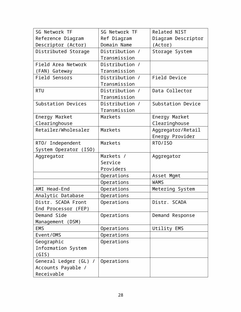
3.2 List of ActorsTable 1 maps the actors included in the SG Network TF Smart Grid Conceptual Reference Diagram (Figure 3) and the NIST smart grid conceptual reference diagram (Figure 1). The SG Network TF high level list of actors are further qualified by domain and sub-domain as used in documenting the Smart Grid business functional and volumetric requirements.

Table 1: Mapping of actors to domain namesSG Network TF Reference Diagram Descriptor (Actor)

SG Network TF Ref Diagram Domain Name

Related NIST Diagram Descriptor (Actor)

Field Tools Customer / DistributionGenerators Bulk Generation Generators Market Services Interface Bulk Generation Market Services InterfacePlant Control Systems Bulk Generation Plant Control Systems

Customer Electric StorageCustomer Energy Management System (EMS)

Customer Customer EMS

DERs (Solar, Wind, premise generation sources)

Customer Distributed Generation

ESI (3rd party) Customer Energy Services InterfaceESI (Utility) Customer Energy Services InterfaceESI (In meter) Customer Energy Services InterfaceElectric Vehicle Service Element (EVSE) / End Use Measurement Device (EUMD)

Customer Customer Equipment

Heating, Ventilating, and Air Conditioning (HVAC)

Customer Customer Equipment

IHD (In Home Device) Customer Customer EquipmentLoad Control Device Customer Customer EquipmentPCT Customer ThermostatPHEV Customer Electric VehiclePhone/Email/Text/Web Customer Customer EquipmentSmart Appliances Customer AppliancesSmart Meter Customer MeterSub-Meter Customer Customer EquipmentTwo Way Meter - Electric Customer MeterTwo Way Meter - Gas Customer MeterTwo Way Meter - Water Customer MeterCapacitor Bank Distribution Field DeviceCircuit Breaker Distribution Field DeviceRecloser Distribution Field Device

19

SG Network TF Reference Diagram Descriptor (Actor)



Distributed Customer Generation

Distribution Distribution Generation

Distributed Customer Storage Distribution Storage SystemSectionalizer Distribution Field DeviceSwitch Distribution Field DeviceVoltage Regulator Distribution Field DeviceDistributed Application Controller (DAC)

Distribution / Transmission

Substation Controller

Distributed Generation Distribution / Transmission

Distributed Generation

Distributed Storage Distribution / Transmission

Storage System

Field Area Network (FAN) Gateway

Distribution / Transmission

Field Sensors Distribution / Transmission

Field Device

RTU Distribution / Transmission

Data Collector

Substation Devices Distribution / Transmission

Substation Device

Energy Market Clearinghouse Markets Energy Market Clearinghouse

Retailer/Wholesaler Markets Aggregator/Retail Energy Provider

RTO/ Independent System Operator (ISO)

Markets RTO/ISO

Aggregator Markets / Service Providers

Aggregator

Operations Asset MgmtOperations WAMS

AMI Head-End Operations Metering SystemAnalytic Database OperationsDistr. SCADA Front End Processor (FEP)

Operations Distr. SCADA

Demand Side Management (DSM)

Operations Demand Response

EMS Operations Utility EMSEvent/OMS Operations Geographic Information System (GIS)

Operations

General Ledger (GL) / Accounts Payable / Receivable

Operations

20

SG Network TF Reference Diagram Descriptor (Actor)



Load Management System (LMS)

Operations

MDMS Operations MDMSNMS Operations RTO SCADA Operations RTO SCADA Trans. SCADA FEP Operations Trans. SCADA FEP Utility Distribution Management System (DMS)

Operations DMS

Utility EMS Operations EMSWork Management System Operations Bill Payment Orgs/Banks Service Provider OtherCommon Web Portal-Jurisdictional

Service Provider Other

Home/Building Manager Service Provider Home/Building Manager Internet/Extranet Gateway Service ProviderODW Service Provider REP CIS/Billing Service Provider Retail Energy Providers

BillingREP CIS/Billing Service Provider Retail Energy Providers

CISUtility CIS/Billing Service Provider Utility CISUtility CIS/Billing Service Provider Utility BillingWeb Portal Service Provider

3.3 Smart Grid Use CasesFrom the Interoperability Knowledge Base (IKB),

http://collaborate.nist.gov/twikisggrid/in/view/SmartGrid/InteroperabilityKnowledgeBase#Use_Cases

use cases come in many shapes and sizes. With respect to the IKB, fairly comprehensive use case descriptions are used to expose functional requirements for applications of the Smart Grid. In order to provide this depth, these use cases contain the following:

Narrative: a description in prose of the application represented including all important details and participants described in the context of their activities

Actors: identification of all the persons, devices, subsystems, software applications that collaborate to make the use case work

Information Objects: defines the specific aggregates of information exchanged between Actors to implement the use case

Activities/Services: description of the activities and services this use case relies on or implements

Contracts/Regulations: what contractual or regulatory constraints govern this use case

21

Steps: the step by step sequence of activities and messaging exchanges required to implement the use case

For use cases following this description, see: http://collaborate.nist.gov/twiki-sggrid/bin/view/SmartGrid/IKBUseCases

SG-Network TF performed an exercise to research and to identify all pertinent use cases that involve network communication to help satisfy the OpenSG input requirements into the NIST PAP 2 tasks. Use cases from several sources (Southern California Edison, Grid Wise Architectural Console, Electric Power Research Institute and others) were researched. Table 2 summarizes the use cases SG-Network TF has currently in scope for this work effort.

Table 2: OpenSG SG Network TF Use Cases and Status

Smart Grid Use Case

Requirements in Release 4.0 of the Requirements Table, or planned for later release(s)

Accounting Management YesConfiguration Management YesDirect Load Control YesDistributed Storage YesDistribution Systems Demand Response (DSDR) - Centralized Control YesFault Clear Isolation Reconfigure YesFault Management YesMeter Events YesMeter Read YesPre-Pay Metering YesService Switch YesCustomer Information / Messaging PartialDemand Response PartialDistribution automation support PartialOutage Restoration Management PartialPHEV PartialPremise Network Administration PartialSecurity Management PartialSystem Updates PartialVolt/VAR Management PartialDistributed Generation PlannedField Force Tools PlannedPerformance Management PlannedPricing: Time of Use (TOU) / Real Time Pricing (RTP)/

Planned

22

Smart Grid Use Case

Requirements in Release 4.0 of the Requirements Table, or planned for later release(s)

Critical Peak Pricing (CPP)Transmission automation support Planned

Documenting and describing the in-scope Smart Grid use cases by SG Network TF is contained in the System Requirements Specification (SRS) document. The SG Network TF objective for the SRS is to provide sufficient information for the reader to understand the overall business requirements for a smart grid implementation and to summarize the the business volumetric requirements at a use case payload level as focused on the communications networking requirements, without documenting the use cases to the full level of documentation detail as described by the IKB.

The scope of the SRS focuses on explaining: the objectives, approach to documenting the use cases; inclusion of summarization of the network and volumetric requirements and necessary definition of terms; and guidance upon how to interpret and consume the business functional and volumetric requirements. The latest released version of the SRS is located at

http://osgug.ucaiug.org/UtiliComm/Shared%20Documents/Latest_Release_Deliverables/

with a file name syntax of “SG Network System Requirements Specification vN.doc”,where N represents the version number.

3.4 Smart Grid Business Functional and Volumetric RequirementsThere are many smart grid user applications (use cases) collections of documentation. Many have text describing the user applications (see IKB), but few contain quantitative business functional and volumetric requirements, which are necessary to design communications protocols, to assess, or to plan communication networks. Documenting the detailed actor to actor payloads and volumetric requirements allows for:

aggregation of the details to various levels (e.g., specific interface or network link, a specific network or actor and have the supporting details versus making assumptions about those details) and

allows the consumer of the Requirements Table to scope and customize the smart grid deployment specific to their needs (e.g., which set of use cases, payloads, actors, communication path deployments).

OpenSG_SG Communications_SG Network TF took on the task to document the Smart Grid business functional and volumetric requirements for input into the NIST PAP 2 tasks and to help fill this requirements documentation void. The current SG-Network business functional and volumetric requirements are located at


with a file name syntax of “SG Network System Requirements Specification vN.R.xls”, where N represents the version number and R represents the revision number. This spreadsheet is referred to below as the Requirements Table.

23

Instructions for how to document the business functional and volumetric requirements was prepared for the requirement authors, but also can be used by the consumer of the Requirements Table to better understand what is and is not included, and how to interpret the requirement data. The requirements documentation instructions are located at:


with a file name syntax of “rqmts-documentation-instructions-rN.R.doc”, where N represents the version number and R represents the revision number.

The Requirements Table consists of several major sets of information for each use case: For example:

Business functional requirement statements are documented as individual information flows (e.g., specific application payload requirement sets). This is comparable to what many use case tools capture as information flows and/or illustrated in sequence diagram flows.

To the baseline business requirements are added the:o volumetric attributes (the when, how often, with what availability, latency,

application payload size). Take note that the SG Network TF Requirements Table definition for some terms (e.g. latency) is different than the classic “network link latency” usage. Please refer to the SG Network TF Requirements Documentation Instructions or section 2.2 for the detailed definitions for clarification.

o an assignment of the security confidentiality, integrity, and availability low-medium-high risk values for that application payload.

Payload requirement sets are grouped by rows in the table that contains all the detailed actor to actor passing of the same application payloads in a sequence that follows the main data flow from that payload’s originating actor to primary consuming actor(s) across possible multiple communication paths that a deployment might use. The payload requirements’ sets will always contain a parent (main) actor to actor row and most will contain child (detailed) rows for that requirement set.

Payload communication path (information or data flow) alternatives that a given smart grid deployment might use.

The process of requirements gathering and documentation has been evolutionary in nature as various combinations of additional attributes are documented; use cases added; payload requirement sets added; and alternative communication paths documented. The SG Network TF has defined over 1400 (as of release 4.0) functional and volumetric detailed requirements rows in the Requirements Table representing 165 different payloads for 18 use cases.

SG Network TF intends to continue this incremental version release approach to manage the scope and focus on documenting the requirements for specific use cases and payloads, yet giving consumers of this information something to work with and provide feedback for consideration in the next incremental releases. It is expected that the number of

24

requirements rows in the Requirements Table will more than double if not triple from the current size when completed.

To effectively use the business functional and volumetric requirements, the consumer of the Requirements Table must:

select which use cases and payloads are to be included select which communication path scenario (alternative) is to be used for each of

the main information/data flows from originating actor to target consuming actor specify the size (quantity and type of devices) of the smart grid deployment perform other tweaks to the payload volumetrics to match that smart grid

deployment’s needs

The current Requirements Table as a spreadsheet is not very conducive to performing these tasks. SG-Network TF is building a database that is synchronized with the latest release of the Requirements Table (spread sheet). SG Network TF will be adding capabilities to the database to:

solicit answers to the questions summarized above; query the database; and format and aggregate the query results for either reporting or exporting into other

tools.

The current SG-Network TF Requirements Database and related use documentation are located at

http://osgug.ucaiug.org/UtiliComm/Shared%20Documents/Latest_Release_Deliverables/ Rqmts_Database/

3.5 Use of Smart Grid User Applications’ Quantitative Requirements for PAP 2 TasksAn earlier release of the Requirements Table (i.e., “SG Network System Requirements Specification v2.1” (March 12, 2010)) contained sufficient data for consideration as a partial list of Smart Grid user applications’ quantitative requirements to PAP 2. This version contained three user applications (use cases): meter reading, PHEV, and service switching along with their quantitative (volumetric attributes) requirements.

Subsequent releases of the Requirements Table from SG-Network have also been made available to PAP 2 for their use. Release 4.0 (June 15, 2010)of the SG Betwork TF Requirements Table contains numerous 18 use cases, payloads (applications), communication path options, and associated volumetric requirements data sufficient for a variety of smart grid deployment scenarios as input to PAP 2. As SG Network TF continues to provide incremental Requirement Table releases and eventually completes that effort, that availability of quantified business functional and volumetric data will provide PAP 2 and the reader of this document with a more complete set of smart grid business functional and volumetric requirement data for assessment of any given network standard and technology against. This is not a do it once and it’s done completed type of task.

25

3.6 Adaptation of SG Network TF’s Requirements Table Data for Use in Network Modeling Tools

When examining the detailed records of the Requirements Table and as noted in section 3.4, there are several decisions and selections the consumer of the Requirements Table must make. This section identifies a method for making most of those decisions and selections, and how to adapt the detailed quantified requirements into a form that can be loaded into the wireless model in section 5.2 or into any other traffic modeling or assessment tool.

Method:Step 1 - Determine which use cases (applications) to use.Step 2 - Select which actor to actor interface is to be investigated:

a) which communication pathb) which network link(s).

Step 3 - Identify the applications’ events (payloads) that are to be used.Step 4 - Select one value for metrics where ranges are provided.Step 5 - Assume (and document) values for missing information.Step 6 - Select which type of data analysis method is to be used:

a) aggregation of data volumetrics based on values per a specified time period for input into a static system model

b) simulation of multiple discrete transactions (payloads) retaining each events unique data volumetrics and profiles

Step 7 – Finalize the data preparation tasks based on the selections and assumptions from steps 1-6.

As of April 12, 2010 there were three user applications provided (meter reading, PHEV, and service switching) in the SG Network System Requirements Specification v2.1. The remainder of this section provides an EXAMPLE of using the steps above on the v2.1 4.0 release of the Requirements Table. As the 7 steps are exercised, mentioned above, for a very limited and focused amount of requirements from the Requirements Table will be selected for analysis.. The user of the Requirements Table and this method needs to perform the steps as driven by the specific to the objectives and scope of their assessment.

Example use of the methodStep 1 - Determine which use cases (applications) to use The spreadsheet filter feature can be used on the “Use Case Ref” column to identify and select which uses cases are of interest. For this EXAMPLE exercising of the steps above, all threetwo applications (Meter Rreading, PHEV, and Service Switch) of the available use cases will be used.

Step 2 - Select which actor to actor interface is to be investigated:a) which communication pathUsing a combination of “pivot tables or data pilots” and additional queriesthe filtered view of the Requirements Table for the three two selected applications

26

and reviewing the distinct 2-way communications between the “From” and “To” actors indicates that there are 32 41 unique one directional primary “From-To”actor to actor pairings, excluding all the intermediary actor to actor pairings..

Let us focus on the Data Aggregation Point (DAP) from/to 2-Way Meter actor to actor pairing.

b) which network link

In reviewing the SG Network TF Reference Diagrams (Figure 2 and Figure 3), indicates that there are three network interfaces “MeA”, “MgA”, :MwA” between the DAP and the 2-Way Meters10. Note the term Smart Meter includes both the 2-Way Meter and the ESI – in meter components. There are two independent data flows that identified between the DAP to the electric Smart Meter: “1D’” which is intended to deal with that traffic terminating with the meter metrology, and “5Ba” which is terminating with the ESI module in meters that have ESI modules, plus “1Dg” and “1Dw” for the other two 2-Way Meters. Without getting too technology specific, many technologies for communicating with 2-way meters use one network interface module that “MeA” interfaces to. Consequently, both the “1D” and “5Ba” data flows would traverse across the “MeA” interface.

The vast majority of the communication interfaces included in the Requirements Table are documented as data flows, which can beare further decomposed to specific network actor to actor or actor to network or network to network links. If the modeling effort is intended to focus on ALL traffic that passes across a network link (e.g. “MeA”), for a specific smart grid deployment, then regardless of the payloads or use cases, all business requirements in the Requirements Table that have data flows that traverse this interface for the specific selection of use cases, payloads, and communication paths (deployment topologies),MUST be used in selecting the requirements data for analysis.

For this simple example, let us focus on just the payloads that are targeted touse the 2-Way Meter –Electric actor metrology from the DAP (i.e., “1D” and “1Dg” and “1Dw”) and NOT the traffic with the ESI – In meter component via “5Ba” or the gas “1Dg” or water “1Dw” dataflows.

Step 3 – Identify the applications` events (payloads) that are to be usedUsing the Requirements Table (v2.14.0) filter capabilities :against the previous 2 application filters, applying using any two of the following three two column filters:• “Data Flow Ref” contains “1D”• “Data Flow from Actor” equals “DAP”• “Data Flow to Actor” equals “Smart Meter”10 Smart Grid architectures include the use of AMI technologies which specifies telecommunication capabilities with the meters as being 2-way. Consequently this excludes 1-way meters and meters without any remote communication capabilities. If the user of the Requirements Table want to include 1-way meters into their analysis, then the requirements specific to those 1-way meters will need to be created by the user specify to their needs.

27

would include those events coming from 3 actors: CIS/Billing – Utility IHD if the communications option via ESI –Utility actor “1D +

5Bb + 16Ab” is selected Cust. EMS if the communications option – ESI – Utility actor “1D

+ 5Bb + 16Cb” is selected .For this example let us restrict the events only coming from the CIS/Billing – Utility actor which results in five events are present in the DAP to Smart 2-Way Meter – Electric metrology direction

2 for the meter reading application,o multiple interval meter reading request and o on-demand meter read requests

. 3 for Service Switch application

o cancel service switch operate request,o service switch operate request, ando service switch state request.

0 for all other applications

and aAfter resetting the previous filters immediately prior,and applying using any two of the following three two column filters:• “Data Flow Ref” contains “1D”• “Data Flow from Actor” equals “Smart Meter”• “Data Flow to Actor” equals “DAP”

would include those events going to 3 actors: CIS/Billing – Utility IHD if the communications option via ESI –Utility actor “16Ab +

5Bb + 1D” is selected Cust. EMS if the communications option – ESI – Utility actor

“16Cb + 5Bb + 1D” is selected .For this example let us restrict the events only going to the CIS/Billing – Utility actor which results in ten8 events are present in the Smart 2-Way Meter –Electric metrology to DAP direction

6 4 for meter reading application,o multiple interval meter read data

Commercial / Industrial Gas smart meters, Commercial / Industrial Electric meters, Residential gas smart meters, and Residential electric smart meters.

o on-demand read request app errors, ando on-demand meter read data.

4 for Service Switch applicationo send service switch operate acknowledgment,o send service switch operate failure,o send metrology information after a successful service switch operate, and

28

o send service switch state data. 0 for all other applications

Step 4 – Select one value for metrics where ranges are provided.Use the information from these events (and perhaps others) to calculate the individual contribution of each event in terms of its frequency (Requirements Table: “How Often” values) and its application payload size. Please note that the Requirements Table “Daily Clock Periods” values directly impacts the frequency calculations when the frequency is taken down from say a daily value to an hourly value for specific time blocks in the day, refer to the hourly columns in Table 3 and Table 4 below. Also if the hour of consideration is shifted to an evening hour, the values may or may not change depending upon the “Daily Clock Periods” for that payload (event).

These metrics have either ranges of values or scalar values. An example of a range of values is the multiple interval meter read data (Commercial / Industrial Gas Electric smart meters) where the frequency is 1 – 612 - 24 transactions per day and the size of the data is 1600 200 bytes – 2400 1600 bytes. An example of a scalar value is the send service switch operate failure to DAP where the frequency is 1 trans per 1000 switch operate per day. Since this is an error based on the original number of switch operate commands, we must obtain that event’s frequency information, which is 1 - 50 transactions per 1000 meters per day.

For each of the possible range of values select a value that is meaningful to your particular deployment scenario. The following tables contain example selections of values.

Table 3: Selected values for DAP to Smart meter directionEvent How often

(events/SMMtr/day)How often (events/SMMtr/midday hour)

Size (bytes)

multiple interval meter reading request

25 events / 1000 SMs Mtrs / day

Daily value/11 25

on-demand meter read requests

25/1000 Daily value/15 25

cancel service switch operate request


service switch operate request 50/1000 Daily value/8 25service switch state request 50/1000 Daily value/8 25

Table 4: Selected values for Smart meter to DAP directionEvent How often

(events/SMMtr/day)How often (events/SMMtr/midday hour)

Size (bytes)

multiple interval meter read data

6 events/SM/day If randomized then daily

240011

29

Event How often (events/SMMtr/day)

How often (events/SMMtr/midday hour)

Size (bytes)

(Commercial / Industrial Gas smart meters)

value/24, otherwise depends on fixed hourly periods

multiple interval meter read data (Commercial / Industrial Electric meters)

2412 If randomized then daily value/24, otherwise depends on fixed hourly periods

1600

multiple interval meter read data (Residential gas smart meters)


2400

multiple interval meter read data (Residential electric smart meters)


2400

on-demand read request app errors

(25/1000+*10)/1000 Daily value/15 50

on-demand meter read data 25/1000 Daily value/15 100send service switch operate acknowledgment


send service switch operate failure

1/1000 * 50/1000 Daily value/8 50

send metrology information after a successful service switch operate


11 The range on the interval data responses is driven by the how often the interval data is transmitted, how many meter data points and interval time spans e.g. 60 minutes - 15 minute. The value as intended to be interpreted from the Requirements Table for this payload specific to the “How Often” specified should be 1600. The 2400 would apply for a “How Often” of 4 events /SM/day. This same clarification applies across the other values in this table and Table. Note, this synching against the Requirements Table should not take away from the example of using the method/steps, just clarifying the intended interpretation of the Requirements table.12 Similar to footnote 10, There is a general inverse relationship between one value of the “How Often” range to that of some of the associated “Payload Size” range values. Tthe intended interpretation of the stated payload size of 1600 is associated with a “How Often” value of 12 which ties with 15 minute interval data and 20 data points per interval. This misinterpretation of the Requirements Table should not take away from the example of using the method/steps. SG Network TF will address how to better document the intended interepretation and use of these range of values in the next release of the Requirements table.

30

Event How often (events/SMMtr/day)

How often (events/SMMtr/midday hour)

Size (bytes)

send service switch state data 50/1000 Daily value/8 100

Step 5 - Assume (and document) values for missing information.There is still some information not available from the user applications matrix. For example to calculate the aggregate traffic from a single smart 2_way meter to a DAP, the type of smart 2-way meter is needed; also the number of smart 2-way meters that will be sending their data to a single DAP is needed.

How many Smart 2-Way Meters?o What proportion of types (deployment classifications using the same

network technology) of smart meters? Commercial / Industrial Gas smart meters, Commercial / Industrial Electric meters, Commercial / Industrial Water meters, Residential gas smart meters, Residential electric smart meters, and Residential water smart meters.

Assume the following proportions of types of smart 2-way meters using scenario 1 2 in Table 5 as this example has been filterd to just the electric meters: Table 5: Example 2-way meter deployment classifications and example apportionments2-Way Meter Deployment Classifications Scenario 1 –

meter (%)Scenario 2 – meter (%)

Scenario 3 – meter (%)

Commercial / Industrial Gas smart meters 6.5 2.5Commercial / Industrial Electric meters 17.4 10 5.0Commercial / Industrial Water meters 2.5Residential gas smart meters 6.5 20Residential electric smart meters 69.6 90 45Residential water smart meters 25Total 100 100 100

Quantity of endpoints (meters) per the same technology DAP in a specific deployment geographic area.

NOTE: Some current technology DAPs AMI Networks have design maximum number of endpoints per DAP that typically range from 1,000 – 50,000. Actual deployment quantity of endpoints per DAP will be less than the technology’s maximums based on:

the endpoint density design limits’ thresholds imposed by the network designers to address

application latency requirements and providing “headroom” in the network.

31

For deployments of 100,000 endpoints, multiple DAPs will be required, with the actual quantity of endpoints (e.g. meters) per DAP varying significantly across that 100,000 deployment. When the assessment is focused on the ability of a technology to handle the deployment, two areas of concern arise (i.e., the high density urban areas and the low endpoint density rural areas). One is focused on the handling of all the traffic and the other is being able to extend the reach between the DAP and the endpoints and still provide acceptable application latency and reliability at acceptable cost points.

For example purposes only, let us assume a 1000 endpoints (smart meters) per DAP assessment.

Step 6 - Select which type of data analysis method is to be used:There are at least two common approaches to data analysis that deal with events that occur in time displaying deterministic timings and those with probabilistic distributions:

a) aggregation of data volumetrics based on values per a specified time period for input into a static system model

b) simulation of multiple discrete transactions (payloads) retaining each events unique data volumetrics and profiles

The aggregation of data volumes based on values per specified time periods will be discussed in this step. The simulation approach is further discussed in section 5.

Aggregation of data volumes based on values per specified time periods, carries with it no indication of when those events occur during the time period. Many readers may make the assumption that the events occur evenly across the time period, but it is just that, an assumption. All that can be stated is that during that time period the events are expected to occur at the stated quantity per total period.

When using the “Daily Clock Periods” a better understanding of the quantity of events occurring in that shorter time period is possible, though as in illustrated in Table 3 and Table 4 above, interpolating that value to an hourly value for a specific hour of the day is possible, but carries the same limits to that usage as mentioned above.

An alternative to just these simple “How Often” values is to consider what those values would be for different operating modes that a smart grid deployment might encounter. This might be represented as three different values to account for: normal; medium; and high periods of event occurrence. For the Meter Reading, Service Switch use cases, this might entail:

after new rate structures have been imposed high energy usage billing periods college move ins / move outs or entry or exodus of customers storm events

Whether or not SG Network TF adds this additional level of detail to the Requirements Table, the user of the Requirements Table can modify the requirement data themselves to match their analysis needs and assumptions, but it must be documented.

32

For simplicity, let us disregard the “Daily Clock Periods” and keep the frequency (How Often) based on a 24 hour period, daily values.

Step 7 – Finalize the data preparation tasks based on the selections and assumptions from steps 1-6.

Using the selected values from step 4 and the assumed values from step 5, and assuming that a data analysis method is selected using the aggregatation of data volumetrics to simple per period metrics, the aggregate traffic for each direction is calculated in Table 6 and Table 7 below.

Table 6: DAP to Smart Meter directionEvent How often

(events/SMMtr/day)Size (bytes/event)

Avg. Traffic Load (bytes/SMMtr/day)

multiple interval meter reading request

25/1000 25 0.625

on-demand meter read requests

25/1000 25 0.625

cancel service switch operate request

2/1000 25 0.05

service switch operate request 50/1000 25 1.25service switch state request 50/1000 25 1.25Total 0.152 N/A 3.8

Mean message size (bytes) per event = 3.8 / 0.152 = 25 bytes/eventNumber of events per meter per second = 0.152 / 86400 = 1.76 x 10-6 events/SMmtr/s

Table 7: Smart Meter to DAP directionEvent How often

(events/SMMtr/day)

proportion Size (bytes/event)

Avg. Traffic Load (bytes/ SMMtr/day)

multiple interval meter read data(Commercial / Industrial Gas smart meters)

6 0.065 2400 936

multiple interval meter read data (Commercial / Industrial Electric meters)

24 0.174 1600 6681.6

multiple interval meter read data (Residential gas smart meters)

6 0.065 2400 936

multiple interval meter read data (Residential electric smart

6 0.696 2400 10022.4

33

meters)Subtotal Frequency *

proportion =9.1328.352 events/ SMMtr/day

Frequency * Size * proportion =

18576 16704 bytes/ SMMtr/day

on-demand read request app errors

(25/1000+*10)/1000 50 0.5012500125

on-demand meter read data 25/1000 100 2.5send service switch operate acknowledgment

2/1000 25 0.05

send service switch operate failure

1/1000 * 50/1000 50 0.0025

send metrology information after a successful service switch operate

2/1000 100 0.2

send service switch state data 50/1000 100 5Subtotal 0.0789 N/A 8.2547.754Total 9.228.43

events/SMMtr/dayN/A 18584

16712 bytes/ SMMtr/day

Mean message size (bytes) per event = 18584 16712 / 9.228.43 = 2016 1982 bytes/eventNumber of events per meter per second = 9.228.43 / 86400 = 1.07 9.76x 10-5 4 events/SMMtr/s

3.7 SecuritySecurity can be considered at every layer of the protocol stack, from the physical layer to the application layer. To consider security in the context of PAP 2, which is mainly concerned with the physical and media access control layers, implies the inclusion of additional protocol and traffic events to achieve security signaling functionality as in the case of authentication and authorization, and additional bytes to existing payloads to achieve encryption. As a first step towards this goal, the SG Network TF Requirements Table lists the Security CIA’s for each event. As a second step, a mapping between these CIA levels and the security protocols available at the various network layers is needed in order to fully address security in the context of PAP 2.

34

4 Wireless TechnologyPAP#2’s Task 5 calls for the collection of an inventory of wireless technologies. This inventory of wireless technologies is captured as a spread sheet, Wireless Functionality and Characteristic Matrix for the Identification of Smart Grid Domain Applications, which can be found on the PAP#2 web site:

http://collaborate.nist.gov/twiki-sggrid/bin/view/SmartGrid/PAP02Wirelesswith a file name syntax of “Consolidated_NIST_Wireless_Characteristics_Matrix-VN.xls”, where N represents the version number.

Disclaimer: The spread sheet was created and populated by the Standards Setting Organizations (SSO), which proposed their wireless technologies as candidates for the smart grid. The parameters and metrics contained and values entered for each wireless technology were done by proponents for that technology. The values were not verified by PAP#2.

The next sections give a brief description of the parameters and metrics contained in the spread sheet, Wireless Functionality and Characteristic Matrix for the Identification of Smart Grid Domain Applications and a listing of the technologies submitted so far.

4.1 Technology Descriptor HeadingsTo be able to describe wireless technology a set of characteristics were identified and organized into logical groups. The group titles are listed below.

• 1. Link Availability• 2. Data/Media Type Supported• 3. Coverage Area• 4. Mobility• 5. Data Rates• 6. RF Utilization• 7. Data Frames & Packets• 8. Link Quality Optimization• 9. Radio Performance Measurement & Management• 10. Power Management• 11. Connection Topologies• 12. Connection Management• 13. QoS & Traffic Prioritization• 14. Location Characterization• 15. Security & Security Management• 16. Radio Environment• 17. Intra-technology Coexistence• 18. Inter-technology Coexistence• 19. Unique Device Identification• 20. Technology Specification Source• 21. Deployment Domain Characterization• 22. Exclusions

35

4.2 Technology Descriptor DetailsEach of these groups was composed of individual descriptive components for which an entry for each technology was requested. The rows are described in more detail below.

4.2.1 Descriptions of Groups 1-7 Submissions

Wireless Functionality and Characteristics Matrix for the Identification of Smart Grid Domain Application

Functionality/Characteristic Measurement Unit

Group 1: Link Availability

a:Ability to reliably establish an appropriate device link % of time

b: Ability to maintain an appropriate connection failure rate per 1000 sessionsGroup 2: Data/Media Type Supported a: Voiceb: Data Max user data rate per user

in Mb/sc: Video Max resolution in pixels @

x fpsGroup 3: Coverage Area a: Geographic coverage area km2

b: Link budget dBGroup 4: Mobility a: Maximum relative movement rate m/sb: Maximum Doppler HzGroup 5: Data Rates a: Peak over the air uplink data rate Mb/sb: Peak over the air downlink data rate Mb/sc: Peak goodput uplink data rate Mb/sd: Peak goodput downlink data rate Mb/sGroup 6: RF Utilization a: Public radio standard operating in unlicensed bands GHz L/ULb: Public radio standard operating in licensed bands GHz L/ULc: Private radio standard operating in licensed bands GHz L/ULd: Duplex method TDD/FDDe: Bandwidth kHzf: Channel separation kHz

g;Number of non overlapping channels in band of operation

h: Spectral Efficiency bits/s/Hzi: Cell Spectral Efficiency bits/s/Hz/cellGroup 7: Data Frames and Packets

36

Wireless Functionality and Characteristics Matrix for the Identification of Smart Grid Domain Application a: Frame duration msb: Maximum packet size bytesc: Segmentation support Yes/No

4.2.1.1 Group 1: Link AvailabilityThe desire is to be able to use the radio link whenever it is needed by the application. There is an expectation that the radio link will not be continuously maintained and that some devices will be “put to sleep” for periods of time and then, upon “wake up” be required to connect to another device on the network to transfer control information or data. Since there is no absolute certainty that a link will be fully operational there is a probability associated with the connection. The technology “Operating Point” chosen is presumably chosen recognizing that a high % availability is desired.

During the period when a radio link is active there is, again, no guarantee that the link will be flawlessly maintained. The failure source is not defined but is presumed to be associated with the failure of the radio to decode properly the radio symbols causing a packet error. Failure could also be caused by interference from other radio sources or perhaps deep fading due to shadowing, but these effects are not explicitly included in the failure calculations. Rate is another way to represent the statistical nature of a radio link. The technology “Operating Point” chosen is presumably chosen recognizing that achieving a low failure rate is desirable.

4.2.1.2 Group 2: Data/Media Type SupportedInformation transferred within the Smart Grid is usually associated with data. However, it was noted that there would be value in transferring both voice and video information. Voice: There is no specification of the codec being used but the assumption was that some form of packetized voice processing would be used and the connection would be two-way.Data: is a generic term for information being transferred from machine to machine and can include information being displayed to a person for interpretation and further action.

Video: Especially in cases where there is an outage and the situation in the field needs to be displayed to others remote from the outage site, video is desirable. Video could be still pictures or motion pictures. The request is that the best case capabilities be reported.

4.2.1.3 Group 3: Coverage AreaWireless systems are designed to service a wide variety of application scenarios. The intent of this group is to capture the expected coverage area in a typical deployment. Some systems are optimized for very short ranges, perhaps 10 meters or less, while others are intended for longer ranges, perhaps on the order of 30 km.The intent of this group is to capture the expected coverage area in a typical deployment.

4.2.1.4 Group 4: Mobility

37

Some Smart Grid applications might require relative movement between a transmitter and receiver during the operation of the radio link. The inability of the radio link to operate successfully in situations of movement is due to Doppler shift. This metric is intended to display the mobility capability of the radio technology in one or both of the two ways commonly used:

a. Maximum relative movement rate (expressed in meters/second)b. The maximum tolerated Doppler shift (expressed in Hertz)

4.2.1.5 Group 5: Data RatesData rates are a very frequently used metric of radio link capability. The data rates for wireless technologies can span 6 decades of range starting at a few kilo bits per second up to several giga bits per second. However, data rate can be considered to be an ambiguous term unless the terms of use are fully described. An additional complication comes from the fact that the data payload of interest is “surrounded” with additional bits used to provide error correction, error detection, address information and a variety of pieces of control information. Because of these added bits the data payload may be a small portion of the total number of bits transmitted and received. The metrics used for this group are therefore in two subsets.Peak over the air data rates are intended to display the data rates of the PHY when sending bits through the air from transmitter to receiver.Goodput is intended to display the rate at which “application data” is being transferred. Goodput rate calculations remove such items as PHY and MAC preamble, address and error correction from the calculation. A Goodput data rate will always be less than the over the air rate used to send data.

Additionally, some radio systems are designed with uplink and downlink data rates that are equal in both directions, as well as others that allow asymmetric rates. Downlink (see terms and definitions) represents the data transmission from the “central” transmitter to the client device receiver. Uplink (see terms and definitions) represents the data transmission from the client device transmitter to the “central” receiver. Typically the asymmetry is designed to provide a higher downlink rate than uplink. This allows a “central” station or base station to take advantage of antenna height and transmit power not available on the client device.

4.2.1.6 Group 6: RF UtilizationThis group asks for display of information on radio spectrum use.

a) Public Radio standard operating in unlicensed bandb) Public Radio standard operating in licensed bandc) Private Radio standard operating in licensed band

Some radio spectrum is available without license fees and is shared among a wide variety of devices. An example of this would be the 2.4GHz ISM band which is generally available anywhere in the world but shared among diverse radio technologies, such as cordless phones, 802.11 Wireless Local Area Networks (WLANs), 802.15 Personal Area Networks and Bluetooth devices, to name a few.

38

Some spectrum is sold and licensed to individual entities, such as a mobile phone service provider, and the designated spectrum (at least on a regional basis) is not expected to be used by any other radio type.

d) Duplex method - It is also generally assumed that Smart Grid radios will be both transmitting and receiving information. One method used to accomplish bi-directional transfer is time division duplexing (TDD) where uplink and down link packets are alternated in time. Another method is frequency division duplexing (FDD) where uplink and downlink packets are carried on different frequencies.

e) Channel Bandwidth - As with data rates, some radios use a very small amount of radio spectrum for their channel bandwidths (perhaps a few kilohertz) while others may use a very large swath (perhaps several GHz).

f) Channel Separation - This metric is intended to report the separation between channels.

g) Non-overlapping channels in the bandTo use an example, some 802.11 radios operate in the 2.4GHz unlicensed ISM band. Within the US there is 83.5MHz of spectrum available; however, there are restrictions on “out of band emissions”. (Described in FCC Title 47). 802.11 initially chose to use a spread spectrum technology that occupied 20MHz of channel bandwidth. When the FCC rules and the technology choices are combined, the result is a technology that has 11 operating channels defined with center carrier frequencies separated by 5 MHz. Hence, in the 2.4 GHz band, 802.11 technology would be described as having 11 operating channels, separated by 5 MHz and 3 non-overlapping channels.

h) Spectral efficiency (bits/second/Hz) - This is a measure of the efficiency of use of the spectrum. It is highly dependent on the modulation scheme being used. Although the differences between over-the-air and usable data described under “Group 4 - data rate” could be repeated here, the intent for this study is only to represent over-the air information. As an example, a radio system operates at a nominal 1800 MHz with a signal that uses 10 kHz of spectrum (Channel bandwidth) to transfer 10 kb/s of signal information, plus has a spectral efficiency of 1 bit per second per Hertz.

i) Spectral efficiency (bits/second/Hz/cell) - By default a simple monopole antenna generates an isotropic pattern with equal transmit and receive gain equal in all directions. Some systems employ narrow band antenna technology to allow the otherwise circular coverage area to be subdivided into “sectors”. Each sector then services its own group of radios independently. Although the “central” station requires a separate antenna for each sector the scheme allows for a greater number of client devices per area of coverage.

4.2.1.7 Descriptions of Groups 1-7 SubmissionsGroup 7: Data Frames and PacketsThis group asks for display of information on packetization process.

a) What is the maximum frame duration?b) What is the maximum packet size that can be sent in one radio frame?

39

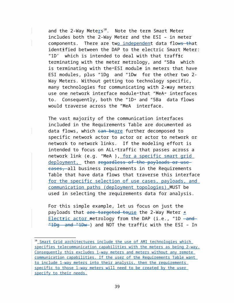
c) Does the radio system support segmentation when the payload size exceeds the capacity of one radio frame?


Group 8: Link Quality Optimization a: Diversity technique antenna, polarization,

space, timeb: Beam steering Yes/Noc: Retransmission ARQ/HARQ/-d: Error correction techniquee: Interference cancellationGroup 9: Radio Performance Measurement & Management a: RF frequency of operationb: Retriesc: RSSId: Lost packetsGroup 10: Power Management a: Mechanisms to reduce power consumptionb: Low power state supportGroup 11: Connection Topologies a: Point to pointb: Point to Multipointc: Broadcastd: MESHGroup 12: Connection Management a: Handoverb: Media Access Methodc: Discoveryd: Association

4.2.2.1 Group 8: Link Quality OptimizationRadio systems can use a variety of techniques to improve the likelihood a transmitted packet will be successfully received. The most fundamental technique is to have the receiving radio send an acknowledgement (ACK) back to the transmitting station. If the ACK is not received then the transmitter will try again (up to some limit of retries). Other techniques seek to improve the signal to noise ratio (SNR) at the receiver. The techniques include polarization, beam steering, etc. The intent here is to capture the techniques employed by the candidate systems.

4.2.2.2 Group 9: Radio Performance Measurement & ManagementThis group is used to indicate what the radio technology provides to an administrator to assist in link assessment. Most radio systems dynamically and autonomously assess their environment and adjust to optimize performance. Sometimes it is useful for an network administrator to monitor behavior to determine if problems exist that are impeding

40

performance or perhaps make manual selections that might indeed improve radio performance beyond what might be achieved autonomously.

4.2.2.3 Group 10: Power ManagementRadio devices may not be directly powered by mains power supply and may be required to run off a battery that is seldom, if ever, recharged. The intent is to capture information on techniques the radio technology has defined that can be used to reduce power consumption.

4.2.2.4 Group 11: Connection TopologiesRadio systems may be designed to use one or more connection topology. One form that is often used is the star topology.

Common topologies

Bus Ring

Mesh

Star

4.2.2.5 Group 12: Connection ManagementThis group is intended to capture the capabilities provided to initiate and maintain radio connectivity.


Group 13: QoS and Traffic Prioritization a: Traffic priority diffserv, resservb: Pass-thru Data Taggingc: Radio queue priorityGroup 14: Location characterization a: Location awareness (x,y,z coordinates)b: Ranging (distance reporting)Group 15: Security and Security Management a: Encryption Algorithms supportedb: Authenticationc: Replay protectiond: Key exchange Protocols supportede: Rogue node detectionGroup 16: Radio Environment

Channel modelInterference sources

Group 17: Intra-technology Coexistence

41

a: Co-channel interferenceb: Adjacent channel interferencec: Alternate channel interferenced: Collision avoidancee: Protection mechanismsGroup 18: Inter-technology Coexistence a: Sensitivity to other interfering radio technologiesb: Degree of interference caused to other radio technologiesc: Sensitivity to power line RF emissionsGroup 19: Unique Device Identification a: MAC addressb: SIM cardc: Other identityd: Rogue detectionGroup 20: Technology Specification Source a: Base Standard SDO SDO name

b:Profiling and Application Organizations Association / Forum

Name

4.2.3.1 Group 13: QoS and Traffic PrioritizationQuality of service can be viewed as and end-to-end requirement, but some radio systems assist in the process by providing QoS between radio nodes. This group is used to capture information regarding the capabilities to manage traffic priority.

a. Traffic priority refers to the ability of radio systems to use high level priority schemes such as diffserv (defined by Internet Engineering Task Force (IETF) RFCs 2472 & 2475) & intserv (defined by IETF RFCs 1633 & 2205).

b. Pass-thru Data tagging refers to the ability to transfer successfully packets that use a class of service priority tags, such as those defined by IEEE 802.1p

c. Radio queue priority refers to the ability of radio nodes to prioritize packets that are queued for transmission.

4.2.3.2 Group 14: Location characterizationRadio systems that provide information about their location can be helpful. One common form of location information would provide 3-dimensional information regarding position, such as that provided via GPS coordinates. An alternate form would provide range information such that when the absolute location of every node is not known, if the location of one radio device was known, then at least the distance between the nodes could be provided.

4.2.3.3 Group 15: Security and Security ManagementEnsuring that Smart Grid data is transferred securely is a high priority. As with other such as QoS there are options to apply security at multiple different layers in the OSI model. This group focuses on options provided and by the radio system at layer 1 and layer 2.

4.2.3.4 Group 16: Radio Environment

42

4.2.3.5 Group 17: Intra-technology CoexistenceSome radio technologies provide mechanisms for avoiding or detecting interference cause by other radios of the same type within receiving range. The intent is to determine if a system has such capabilities that can be used to reduce detrimental interference and thereby improve SNR, and thus will allow the radio to maintain a low error rate link.

4.2.3.6 Group 18: Inter-technology CoexistenceAs with the previous group, some radio technologies provide mechanisms for avoiding or detecting interference cause by other radios of a different type that are operating in the same spectrum and are within receiving range. The intent is to determine if a system has such capabilities that can be used to reduce detrimental interference and thereby improve SNR, and thus will allow the radio to maintain a low error rate link.

4.2.3.7 Group 19: Unique Device IdentificationIt was desired that each radio node be directly identifiable and addressable. This requires that each device have a unique identification scheme. There is more than one way to accomplish this. The information provided will identify the unique identification scheme offered.

4.2.3.8 Group 20: Technology Specification SourceThe intent is to provide information about the SDO that developed and maintains the radio technology, plus identify who provided the information for the matrix. Also, in some cases the base standard source is assisted by a compatriot organization that provides additional support including specifications or applications that operate above Layer 2. The support organizations may also provide certification of specification compliance, interoperability and performance.

4.2.4 Descriptions of Group 21 Submission

Wireless Functionality NOT directly specified by a standard that is needed in quantifying operating metrics

Rx sensitivity dBmTx Power peak dBmAntenna gain dBiNoise floor dBmModulation GFSK, OFDM,

BPSK, GMSKForward error Coding Coding rate

4.2.4.1 Group 21 DescriptionAlthough these items are vital components of a radio technology description, they do not directly affect the suitability of a technology to a Smart Grid application.

They are a few additional characteristics that are needed to characterize the operation of the radio for the chosen operating point.

43

Rx sensitivity - Receiver sensitivity may be specified as a minimum capability required by the SDO in the technology specification. Technology implementations may provide much greater sensitivity than the minimum, so the intent is to capture a typical value that is used for the operating point calculations.

Tx Power peak – Transmission Peak power is needed for the calculations as well. Some technologies specify only a regulatory limit or allow for a wide variety of options. The Tx power of the devices under consideration for the operating point calculations needs to be specified.

Antenna gain - Antenna gain is rarely part of a technical radio standard but is a critical component of link budget calculations.

Noise floor - Noise floor is much like receiver sensitivity. There might be a minimal specification for noise floor required by the SDO in the technology specification. Technology implementations may provide a much lower noise floor than the minimum, so the intent is to capture a typical value that is used for the operating point calculations.

Modulation - The modulation scheme is not directly part of any calculation but needs to be indentified to aid in other technologists verifying the operating point calculations were correct.

Forward Error Coding - The methods used by the technology are not of direct interest but the coding rate is when trying to understand the difference between over-the-air data rates and Goodput rates.

4.3 Technology Submission TitlesResponses have currently been received for the following technologies:

• Cdma2000 1x and cdma2000 High Rate Packet Data (HRPD)• Cdma2000 xHRDP• Geo Mobile Radio 1 (GMR-1) Third Generation (3G)• Internet Protocol over Satellite (IPOS) /Digital Video Broadcast (DVB)-S2• Regenerative Satellite Mesh - A (RSM-A)• IEEE 802.16 e,m• IEEE 802.11• IEEE 802.15• Inmarsat Broadband Global Area Network (BGAN)• Long Term Evolution (LTE)• Evolved High-Speed packet Access (HSPA+)• Universal Mobile Telecommunications Systems (UMTS)• Enhanced Data rates for GSM Evolution (EDGE)• Bluetooth

5 Modeling and Evaluation Approach

Determining an assessment method for evaluating whether a wireless technology can satisfy the smart grid user applications’ requirements is a daunting task, especially given that there are many possible physical deployment options for smart grid devices and facilities, many wireless technology standards, and uncertainty in planning for future needs.

44

Some wireless technologies are a part of a larger system, while others are complete communication networks. For example, wireless technologies developed by the IEEE 802 working group consider mostly the Media Access Control (MAC) sublayer and Physical Layer (PHY), while the Universal Mobile Telecommunications System (UMTS) is a complete mobile (and wireless) network system. This makes comparing wireless technologies impractical. For this reason, PAP 2 assesses each wireless technology on whether it can satisfy the smart grid user applications requirements; PAP 2 will not rank the various wireless technologies relative to each other.

5.1 Assessment of Wireless Technologies Against Smart Grid Business Application Requirements

The assessment approach described below should be considered as an approach, not the approach that must be used. Options are discussed on how the assessment can be refined with one method further described and detailed in this section’s sub-sections. The two main tasks are:

1) Perform an initial screening of the wireless technologies against the Smart Grid Business Functional and Volumetric Requirements and

2) Perform refinements to the initial screening using one or a combination of the following:

Mathematical models Simulation models Testbeds (lab and in the field)

5.1.1 Initial screeningThe initial assessment (technology screening) is based on the smart grid user applications’ requirements in Section 3.4 and the wireless functionality and characteristics matrix in Section 4. For example, a user application’s requirement for reliability should be related to the wireless technology’s link availability (i.e. the ability to reliably establish an appropriate device link and the ability to maintain an appropriate connection). One can use the results from the initial assessment to determine whether a given wireless technology should be further considered for use with a particular application in a particular deployment.

5.1.2 Perform refinements to initial screeningAfter the initial assessment, the next step is to refine the assessment using other methods (i.e., mathematical models, simulations models, or testbeds).

5.1.2.1 Mathematical Models These types of models require creating mathematical model representations that approximate the characteristics of the system in question (e.g., the Smart Grid). These models can be simplistic in that event data volumetrics are aggregated to singular values, or events are treated as individual inputs into the models, or data volumetrics represented and input based on probabilities. Mathematical models usually take less time to produce results than simulation models. There are some limitations to what some of the simpler mathematical models can adequately model.

45

5.1.2.2 Simulation Models These types of models, attempt to account for more of the event occurrence variability as noted in the mathematical model discussion above. Simulation models can provide more realistic results than mathematical models, which often require simplifying assumptions to make them tractable.

5.1.2.3 TestbedsUsually, neither mathematical or simulation model types are able to capture most of the details of a proposed network deployment (e.g., accurate channel models are difficult to obtain without direct measurement of the deployment environment). Using testbeds (in the lab and preferably actual in the field), can provide very accurate results; however, this method requires the most time, effort, and resources to produce results.

The key for network design is to understand and define the networks system design goals. Designing a network system to support the average data requirements is one design concept, which tends to result in under designed and built networks. Another concept is to design network systems that can handle the absolute worst case imaginable, which tends to result in over designed and built networks. Again the key is to establish a goal of the network and of the individual elements and threads of that network so that it will handle the heaviest expected (combined) burst rates with an acceptable level of failure. For example, in the old telephone trunk design days, one would specify the number of voice trunks necessary to carry the “busy hour” traffic with an acceptable level of failure (2% failure, 5% failure, etc.).

This then leads to two questions that the network designers and implementers need to address, but are not answered in this guideline:

1) What is this highest level of traffic that must be accommodated over the burst period(s)?

a. The methods for determining this will be highly dependent on the individual utility operational modes and the aggregated data that will flow through a particular network link or thread. As you can imagine, this will vary greatly from utility to utility and with the topology/technology used to construct the network threads.

2) What is an acceptable level of overloading these threads that will result in failure to deliver the data within the required latency and fidelity constraints?

a. This will depend on multiple factors, including the latency and fidelity requirements of the system or application, buffering capabilities to buffer overflow traffic, and how error recover is accomplished.

The Utilities will need to implement systems that will satisfy the needs of that specific utility. Translation – one size does not fit all. So the network designers need to find a way to project and predict the real temporal (and spatial) requirements of the data flows (for the utility, application, or operating mode in question) and to then select and implement technologies and topologies that will provide the needed capacity, reliability, security, cost effectiveness, etc.

46

For illustrative purposes, a general modeling framework was developed by the PAP2 working group. It is described below, with additional detail provided in references. Following the description is an example mathematical model showing how the modeling framework can be used.

5.2 Modeling Framework The goal of the development process was to produce an analytical structure that was flexible so that it allows users to employ a variety of modeling techniques, and it can be used with virtually any proposed wireless technology. The framework’s main components are a MAC sublayer model, a PHY layer model, a module that performs coverage analysis, a channel propagation model, and a network (NET) model. The overall design of the model is shown in Figure 4. This subsection discusses each of these components and explains how they interact with each other and operate within the larger analytical framework.

ProbabilityTx Failure

Requ

ireme

ntsOu

tput

Appli

catio

n

DistanceTx-Rx

PHYModel

SNR

Appli

catio

n Req

uirem

ents

Inpu

t

SINR

Number of Devices

Message Frequency

Message Size

Environment

Outage Prob.

Net Reliability

Net Delay

Net Throughput

RoutingTop. Link Reliability

Link Delay

Link Throughput

ModelPropagation

Channel

Path Loss

Model

AnalysisCoverage

Max. OutageProb.

Max. Tx-Rx Dist.

Wire

less T

echn

ology

Inpu

ts

MACModel

ModelNET

Figure 4 – Modeling Framework Building Blocks

5.2.1 Channel Models

Channel models represent the electromagnetic environments that affect the characteristics of a communications signal along the wireless propagation path between a transmitter and receiver. Characteristics which are of greatest interest to the wireless communications designer are the attenuation and the time dispersion of the signal, which can compromise its integrity at receiver.

47

The path loss quantity L models the attenuation of the signal in terms of the fraction of the received power to the transmitted power at the antennas. The deterministic component of the path loss Ld is a function of the distance d (m) between the pair. The widely accepted model in the wireless propagation community is exponential attenuation in function of distance according to a path loss exponent n0. However, in many environments, the degree of exponential fading increases to n1 after a certain breakpoint distance d1. The breakpoint path loss model below (equivalently shown on a dB scale) is more general to capture this phenomenon:

,

where L0,dB is the reference path loss at d0 = 1 m.

The random component of the path loss Ls,dB = Xs,dB + Xf,dB is composed from two terms. The first term Xs,dB is referred to as shadowing. Shadowing represents the deviation of the signal from its predicted deterministic model due to the presence of large obstructions on the wireless path. Obstructions may be buildings or cars in the outdoor environment or walls or furniture in the indoor environments. These objects have varying size, shape, and material properties which affect the signal in different ways. Xs,dB is modeled as a zero mean Gaussian random variable with standard deviation, . The second term Xs,dB is referred to as fading. Shadowing represents the deviation of the signal due to the presence of smaller obstructions on the path which cause scattering of the signal. The signals then constructively and destructively recombine at the receiver. Xf is modeled as a unit-mean gamma-distributed random variable with variance 1/m (where m is the Nakagami fading parameter) and Xf;dB = 10 log10(Xf ). We assume that the shadowing and fading are constant during the transmission of a frame, are mutually independent, and are independent of those on other links.

The complete path loss model, including both deterministic and random components, is

LdB = Ld,dB(d) + Lr,dB.

Figure 5 shows the path loss model extracted from actual measured data points. The deterministic component in red is fit to the blue data points collected in an indoor-indoor residential environment at fc = 5 GHz. The deviation of the data points from the line reflects the random component.

48

Figure 5 - The breakpoint path loss model in an indoor-indoor residential environment at fc = 5 GHz

5.2.2 Coverage AnalysisThe purpose of the coverage analysis is to predict the maximum range of a wireless technology for a given outage probability and a specified set of operating parameters. The range of a wireless technology can help to determine its suitability for linking a particular pair of actors and its coverage area in a point-to-multipoint arrangement.

The outage criterion is the probability that the wireless transmitter-receiver link is not operational. It is expressed in terms of a probability because of the unpredictable behavior of RF propagation, which is often modeled as a stochastic process when accounting for the possible losses due to obstructions (shadowing) and reflections (multipath fading).

In the context of a point-to-multipoint wireless technology, coverage is often analyzed in terms of the maximum cell radius that a base station (BS) or access point (AP) can support. Within the cell, the outage probability varies, generally increasing as a terminal approaches the cell edge. In the example below, the outage criterion is expressed in terms of the average outage probability, averaged over all locations in the coverage area. Thus, a reported outage probability of 1%, for example, means that a terminal located at a random point in the cell has a 1% chance of being in outage.

We define the outage probability as the probability that the received signal-to-noise-ratio (SNR) is below the required SNR to operate the link. The required SNR depends on the wireless technology under consideration and serves as an input to the analysis. The received SNR is modeled using the path loss model described in Section 5.2.1.

5.2.3 PHY Layer

The purpose of the PHY layer model is to estimate the probability that a transmission attempt fails due to channel errors caused by noise and interference. The transmission failure probability takes into account factors affecting the link budget, including transmission power, antenna gains, channel attenuation, thermal noise, background

49

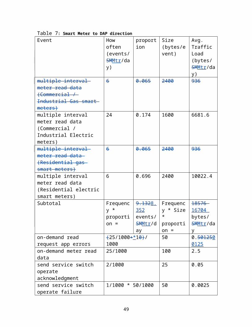
interference, the number of contending stations (if the channel is shared), and the spread spectrum processing gain, if applicable. Depending on the level of modeling, the PHY layer model may also explicitly model the stages of the transceiver, such as channel equalization, demodulation, and forward error correction, resulting in a bit error rate or block error rate. Alternatively, the PHY model may abstract some of these functions and model them with an overall required Eb/N0 (energy per bit to noise power spectral density ratio), wherein the probability of transmission failure is reflected as the probability that the received signal-to-noise-and-interference ratio (SINR) per bit exceeds the required Eb/N0.

As part of the modeling framework, the PHY layer model provides the MAC sublayer model with a conditional probability of transmission failure. For example, with a contention-based MAC, the MAC model supplies the PHY model with the number of contending transmissions. Given the parameters of the link budget and channel statistics, the PHY model then returns the probability that the transmission of interest is unsuccessful conditioned on the number of contending transmissions.

5.2.4 MAC Sublayer

The MAC sublayer model can be either analytical or simulation-based, and its complexity is determined by the preferences and needs of the user. The MAC model receives inputs based on the application requirements and the wireless (or wired) technology that is being used to transport the data; the model interacts with both the PHY layer and the coverage models.

The MAC sublayer model is responsible for returning values for the following performance metrics for the communications system:

Reliability Mean packet delay Throughput

We define the reliability, R, to be the probability that a packet originating from a sending node’s MAC layer is correctly received by the corresponding MAC layer at the receiving node. Thus the reliability is defined with respect to a single link, rather than on an end-to-end or edge-to-edge basis. For MAC layers with a shared channel, where there is contention for resources, the reliability is the probability that the packet does not collide with any packets that are transmitted by other senders and that the packet is not corrupted by channel errors. If the channel is dedicated to the sender (no contention), then the reliability is simply the probability that the packet does not experience any channel errors.

The mean packet delay, D, is the average time from the passage of the packet to the sender’s MAC layer from the protocol layer immediately above to the delivery of the packet by the receiver’s MAC layer to the protocol layer immediately above it. The mean packet delay includes the following:

The time that the packet spends in the sender’s MAC layer’s transmission buffer The processing time at the sender’s MAC layer

50

The time required to transmit the packet, which is the packet length in bits divided by the PHY layer channel rate in bits/s

The time spent waiting to retransmit the packet if it encounters collisions (in the case of a contention-based MAC protocol) or channel errors

The propagation delay between the sender and the receiver The processing time at the receiver’s MAC layer

The throughput, S, is a measure of how efficiently the channel is being used, and it is measured in units of application bits per second. The model computes two types of throughput. The first type is the average throughput, which is the product of the offered load at the application layer, , and the packet reliability, R. Note that this means that the ratio of the throughput to the offered load is always a number between 0 and 1. The second type of throughput measured by the model is the instantaneous throughput, which is the ratio of the mean number of application data bits per packet to the mean packet delay. This gives the effective channel rate experienced by a packet that is ultimately successfully sent across the link, even if it requires retransmissions.

The major external inputs that do not depend on the particular MAC technology are the number of devices accessing the channel, the mean packet generation rate of each device, and the mean packet size. The mean packet generation rate is typically given in units of packets per second; the actual packet generation process is arbitrary. Packets can arrive according to a deterministic process, in which case the mean generation rate is simply the actual generation rate, or they can arrive according to a random process, e.g. a Poisson arrival process. The size of the packet typically includes the size of the application data as well as the combined size of all headers, including the MAC and PHY layer headers. The packet size can be deterministic or random, depending on the applications that are being modeled.

There are additional inputs that are unique to the MAC technology that is being modeled. In the case of a contention-based MAC technology, these parameters can include the number of times the MAC layer will attempt to transmit a packet before giving up and dropping it, rules for handling packet collisions, such as the amount of time that the MAC layer must wait to retransmit a packet after it has collided with a packet from another transmitter, and the amount of time the sending MAC layer must wait for an acknowledgement of a transmitted packet before taking further action. Non-contention MAC technologies will use different parameter sets.

The PHY layer model exports the probability of transmission failure (Pfail) to the MAC sublayer model, which uses it to help compute the output metrics. For instance, if we were modeling a very simple MAC layer that uses dedicated resources (so no contention) and no retransmissions, we would find that the reliability is equal to (1 − Pfail), and the mean delay of successfully received packets is the sum of the propagation delay and the transmission time.

51

The coverage model exports the maximum Tx-Rx distance to the MAC sublayer model. If we have only a user population density, we can use the maximum Tx-Rx distance to compute the size of the user population.

5.2.5 NET LayerWhile the MAC layer model generates the performance metrics per link in a network, the NET layer model works interactively with the MAC to generate the end-to-end performance metrics for collections of links in the network. The MAC performance metrics depend on the amount of contention at a generic station and as a result are a function of the number of contending stations, (i.e. the number of stations within its coverage range). This number is determined in part by the coverage analysis; however, it may vary locally according to the station distribution in the network. The distribution can be defined by a statistical model or given from a real deployment. Given a local population of contenders at a station, the MAC returns the corresponding link performance metrics to the NET. The model synthesizes the link performance metrics to generate network performance metrics for the whole network.

The input parameter to the MAC from the NET is the routing topology. If a destination station lies within the coverage range of a source station, the source can route directly to it. As an alternative if the destination lies outside the range, the source can route to it through consecutive relay stations, each within the range of the previous, in a multi-hop routing topology. Consequently, the local traffic at a relay is particularly sensitive to the selected topology because it depends, not only on it own source traffic generation rate, but also on the amount of traffic generated from forwarding relays.

5.3 An ExampleIn this subsection we use the methodology that we described in the previous subsections to demonstrate how one can begin with a set of traffic characteristics, a physical channel description, and a MAC layer protocol of interest, and arrive at output metrics that quantify the performance of the system. For this example, we consider a hypothetical channel between a population of smart meters and a DAP. The link is loaded with traffic from applications associated with the following three use cases defined in [1]: Service Switch (SS), Meter Reading (MR), and Plug in Hybrid Electric Vehicle (PHEV). In this example, the link uses IEEE 802.11 and features losses due to fading, shadowing, and interference. We begin by considering the input from the application requirements.

Other examples may be found on the PAP#2 web page under Call for input to Task 6. http://collaborate.nist.gov/twiki-sggrid/bin/view/SmartGrid/PAP02Wireless

5.3.1 Link Traffic ModelUsing the requirements of the applications that cross the DAP–smart meter interface, this section illustrates how these requirements can be translated into link traffic characteristics for telecommunications modeling. For example, on the downlink from the DAP to the smart meter (2 way), two applications (creating five events) send traffic across this link. The message generation rates and message sizes of these applications are shown in Figure 6. For the purpose of analysis, we shall assume that the sources can be modeled

52


as independent Poisson processes. Adding up the message rates yields an aggregate message arrival rate of 1.8×10-6 events per electric smart meter (emeter) per second on this link. Furthermore, taking a weighted average of the message size, weighted by the individual message rates, yields an average application message size of 25 bytes. We can repeat this process for the uplink to find the aggregate arrival rate and average message size to be 7.0×10-5 events/emeter/s and 2366 bytes, respectively. Application message rates and sizes obtained similarly for other links can be found in [2].

DAP Smart Meter

MR-25 25/1000 events/meter/day 25 bytes


SS-26 2/1000 events/meter/day 25 bytes



MR-42 25/1000 *X events/meter/day 50 bytes




SS-37 1/1000 * 50/1000 events/meter/day 50 bytes


MR- 25/1000 events/meter/day 2400 bytes

Figure 6 - Application flows from DAP to Smart Meter and Smart Meter to DAP

5.3.2 Coverage AnalysisThe 2.4 GHz ISM band is commonly used in conjunction with IEEE 802.11b/g, the technology considered in this example. Table 8 lists values for the parameters in the equation above that were extracted from measurements made at 2.4 GHz in various environments [3], [4], [5], and [6].

Table 8: Path loss parameters at 2.4 GHz for several environmentsEnvironment L0 (dB) n0 d1 (m) n1 (dB)

Indoor residential LOS 16.3 4.2 N/A N/A 2.4Indoor residential NLOS 12.5 4.2 11 7.6 3.0Indoor industrial NLOS 29.4 3.4 N/A N/A 6.3

Outdoor urban-canyon NLOS 21.3 3.6 N/A N/A 7.4Indoor-outdoor convention center NLOS 4.2 2.6 100 5.7 4.6

Using these channel model parameters, Figure 7 plots sample results for the average outage probability in a circular coverage area as a function of the coverage range. Outage curves for three cases are shown, all at 2.4 GHz: (i) the indoor residential non-line-of-sight (NLOS) environment (row 2 of Table 8) at typical transmit power, (ii) the outdoor urban NLOS environment (row 4 of Table 8) at typical transmit power, and (iii) the same outdoor environment but operating at the maximum permitted Effective Isotropic Radiated Power (EIRP) for the unlicensed 2.4 GHz band. In each case, the fading is

53

Rayleigh (i.e., Nakagami fading parameter m = 1). The values for the remaining technology-specific parameters used in this example are listed in Table 9 and generally correspond to the IEEE 802.11 standard operating at 1 Mb/s. The mathematical expressions used to generate the curves in Figure 7 are detailed in [2].

Table 9: PHY parameter values used for Figure 7PHY data rate 1 Mb/sRequired Eb/N0 10.4 dB

Receiver noise figure 5 dBImplementation loss 1.5 dB

Figure 7 - Sample outage results at 2.4 GHz

Figure 7 shows that, for this example, the outdoor coverage range corresponding to a 1 % outage probability is 220 m at moderate transmission power and nearly 500 m at maximum transmission power. Furthermore, the indoor range is clearly sufficient for most indoor residential environments.

5.3.3 PHY Layer Model

The probability of failure of a transmission attempt is modeled as the probability that the received signal-to-interference and-noise ratio (SINR) is less than a threshold. The received SINR is modeled as random due to channel attenuation (fading, shadowing, path loss) and interference, both of which are treated as random processes. The SINR threshold model for transmission success/failure is based on the observation that for block transmissions the block error probability in the absence of fading and shadowing is a steep function of the SINR. The model approximates this function as a step function at a threshold value of SINR. According to this model, when the actual received SINR—after accounting for fading, shadowing, and the instantaneous interference power—is less than this threshold, the transmission is deemed a failure; otherwise, it is deemed

54

successful. The probability of failure jointly accounts for loss due to a weak received signal, failure due to collision with other stations, and the possibility of capture in the presence of interfering transmissions. Mathematical expressions used in this example for the probability of transmission failure are detailed in [7].

5.3.4 MAC Layer Model

The MAC model used in this example combines elements of the Bianchi and Zhai models of the IEEE 802.11 MAC [8], [9] to produce an extended MAC layer model for the half-duplex channel. This model contains novel elements that allow us to more accurately predict the performance of lightly loaded wireless networks that feature bidirectional traffic patterns on their links. The principal features of this model are described in detail in [7].

Using this model, we analyzed the logical link between a DAP and the smart meters assuming the use of an intervening layer of relays. The relays aggregate traffic from smart meters and send the aggregated traffic to the DAP over an 802.11 wireless multiple access network. Using the physical layer parameter values of Table 9 along with the channel parameters for the outdoor urban NLOS environment in Table 8, our 802.11 analysis tool processed the traffic parameters of the DAP-relay link and returned its mean delay, reliability, and throughput. The number of relays communicating with the DAP was set to 40 in this example, and the smart meters were assumed to be evenly allocated to the relays.

Figure 8 plots the throughput and Figure 9 plots the delay on the DAP-relay link as a function of the number of smart meters served by each relay. The relay-DAP uplink saturates first, because of its higher traffic load, but not until 4000 smart meters per relay. Recalling the coverage analysis of Figure 7, the coverage range at maximum power and 1% outage probability is about 0.5 km. Assuming comparable DAP and relay coverage ranges, and an urban meter density of 2000 electric meters per square kilometer, the DAP would only have about 6000 smart meters within its two-hop coverage area, or about 150 smart meters per relay, far below the link’s capacity limit of 4000 smart meters per relay. Thus, considering all factors—geographic coverage, traffic load, and link performance—we observe that the SM relay-DAP link in this example is coverage-limited, not bandwidth-limited, and therefore has excess network capacity.

The traffic load used in this example is derived from the SS, MR, and PHEV use cases, as described in Section 5.3.1. Additional application traffic will cause the network to saturate at a lower number of meters.

55

Figure 8 - Relay throughput, versus number of SMs aggregated per DAP

Figure 9 - Mean delay of relay and DAP, versus number of SMs aggregated per DAP

5.3.5 NET Layer Model

In this subsection, we provide an overview of the NET layer modeldescribed in [10] . The model serves to extend the deployment range of the stations in a network to beyond the coverage range of the access point. In order to do so, the stations route or hop through multiple relay stations to the access point. The model is used to generate the throughput, reliability, and delay performance metrics for the example in Section 6.5.

The performance metrics of the network can be analyzed by indexing the stations according to the number of hops they require to reach the access point. The indexing is both a function of the distribution of the stations and of the selected routing protocol. In

56

our model, we assume the minimum-hop routing protocol, however our framework is general enough to deal with other protocols such as minimum airtime, minimum bit error, etc.

Once the stations have been indexed according to hops, they are grouped according to their hop index. The stations in each group share parameters such as load. For example, the stations farthest away from the access point in terms of hop distance have the lightest load. This is because there are no stations yet farther away to forward their loads through them. Conversely, the stations closest to the access point must forward the loads of all stations farther away, so their loads are the heaviest. These group parameters are used as inputs to the MAC layer model described in Section 5.3.4. In turn, the performance metrics of the stations in each group are returned as outputs of the MAC layer model by calling it separately for each group. Once the performance metrics of the stations in each group are computed, the network performance metrics are found by averaging those of all the stations.

6 Performance Findings

The purpose of this section is to discuss key performance trends and findings related to wireless communications and how well they support the operational requirements of a smart grid.

Rather than consider every candidate wireless technology in the context of every environment and smart grid application that has been catalogued, and given the need to produce this report in a timely fashion, we choose to focus on key factors that affect performance of most wireless technologies using IEEE 802.11 in the example numerical results. The key factors that we identify as having significant impact on performance include interference, wireless environment, deployment coverage range, and extension of the deployment range. These factors will have to be considered in almost any deployment environment. Thus, we vary each factor over a range of parameter values and discuss the implications that these parameter variations bring with respect to a set of performance metrics. The performance metrics include the application throughput, the reliability (i.e. the probability that the frame can be successfully sent over the wireless link), and the average delay in sending a frame over the wireless link from one node to the next. Note that these performance metrics directly relate to the user requirements that have been compiled for this effort.

It is important to note that the quantitative data based on IEEE 802.11 used in this section is for illustrative purposes only. While the degree to which the environment impacts a particular wireless technology depends on the technology itself and how it is implemented, the general implications of the environmental effects that we discuss will apply to any wireless link-layer technology that could be used to communicate over the link of interest.

6.1 Performance Metrics and User Applications’ Requirements

57

The figures presented in the following subsections show performance metric curves that are representative of the general case. Wherever applicable, horizontal or vertical lines were added in order to show how these curves compare to the user applications’ requirements. In the case of the vertical lines, the threshold is associated with the size of the data and maps into the offered load that is varied on the x-axis. On the other hand the horizontal lines are associated with latency and reliability thresholds provided as part of the user applications’ requirements. It is important to note that the user requirements are measured at the application layer, while the numerical data presented in this section is for the link performance and represents only a component of these requirements. Additional protocol and processing overheads may introduce additional components that need to be considered. For example, the link performance for latency is required to be less than the application latency requirement in order to account for the additional delay components introduced by higher layer functionalities and processing times. For illustrative purposes, we continue to use the example that is described in section 3.6 and section 5.3.1. This example selects the meter reading and service switch use cases and the 1D path (i.e., between DAP and Smart meter). The delay requirement for these events is less than five seconds. The reliability for these events is greater than 98 percent. The calculated throughputs under these conditions are 1.333 bit/s per smart meter on average and 3840 bit/s for a single meter read burst.

6.2 The Effect of Interference The ambient interference on a link, which is distinct from the interference that results from the collision of frames sent by simultaneously transmitting stations, affects the performance of all network elements that are trying to communicate, because it decreases the available link margin. If the margin is degraded enough, transmitted frames will be so severely corrupted that they will be unrecoverable and will have to be resent. This will in turn reduce throughput, decrease reliability, and increase the average frame delay.

We show how the level of ambient interference can affect system performance, using a hypothetical environmental scenario with moderate path loss and shadowing. Detailed parameter values and assumptions used for this scenario and the models used in the evaluation are presented in Section 6.7. We show throughput, reliability, and mean delay in Figure 10, Figure 11, and Figure 12, respectively. In each figure we plot the performance metric versus the offered load (measured in application bits per second) for three values of the ratio of the interference power spectral density to the noise power spectral density. Each figure also features a dash-dotted vertical line indicating the average offered load of a single smart meter operating under normal conditions, and a dotted vertical line indicating the peak offered load per smart meter. In Figure 11 and Figure 12, we use a dashed horizontal line to indicate a lower limit on the reliability and an upper limit on the delay. In practice, these limits would be determined by the network designer based on the smart grid’s operational requirements.

58

Figure 10 - Application throughput versus application offered load for various levels of interference.

Figure 11 shows that we have very poor reliability even at very low loads under moderate and severe interference conditions. For all three levels of interference, when the offered load increases beyond the saturation point, the reliability will decline from its nominal low-load value. We observe that the critical value of the offered load beyond which we see saturation is lower for the highest interference case than it is when the interference is less severe.

59

Figure 11 - Reliability versus application offered load for various levels of interference.

We can also examine the effect of interference using the mean MAC-layer delay in Figure 12. Here the difference in performance between the lower two interference cases is apparent, even at low loads. All three interference scenarios resulted in unacceptable delays at peak offered load. The delay for the highest interference case at low loads is within the limit, but Figure 11 shows that the reliability is unacceptably low.

Again we note that while the numerical values presented in these graphs are applicable only to this example scenario, we can expect to see similar effects for other wireless technologies. The task for the network designer will be to identify the maximum tolerable interference strength for the technologies under consideration and determine, based on the ambient interference in the deployment environment, which subset of technologies are feasible. One must keep in mind that the exact value of the maximum tolerable interference will depend on the environment and the wireless technology that the network operator decides to use.

60

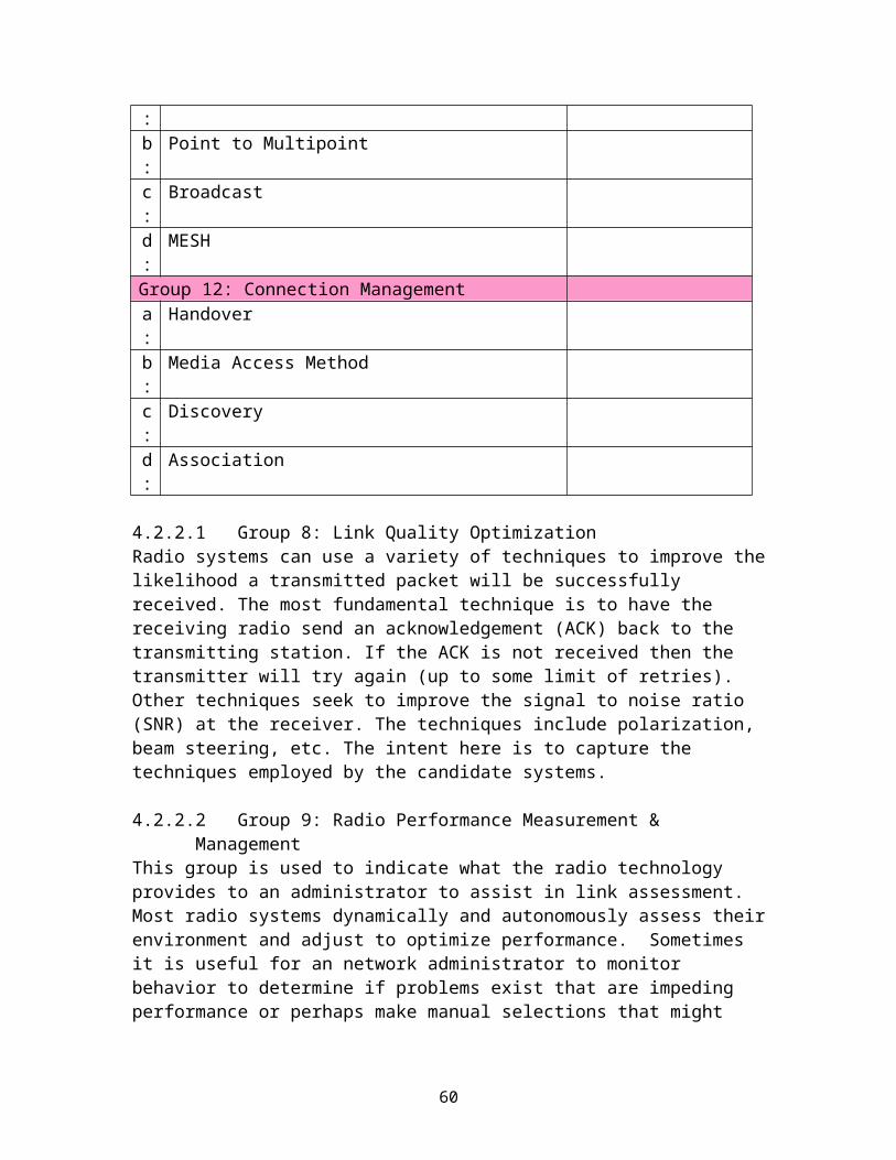
Figure 12 – Mean MAC layer delay versus application offered load for various levels of interference.

6.3 The Effect of the Wireless Link EnvironmentWe have shown that interference can have a significant impact on performance. We now show how a given wireless technology, when used in different operating environments, exhibits different behaviors. In Figure 13, Figure 14, and Figure 15 we show throughput, reliability, and delay curves for three environments, all of whose characteristics are given in Section 6.7. As in Figure 10, Figure 11, and Figure 12 we use a horizontal dashed line to indicate minimum reliability or maximum delay bounds, and we use dash-dotted and dotted vertical lines to show average and worst-case offered loads per smart meter. One environment, which we denote as “rural,” is relatively benign, featuring shallow path loss and low-variance shadowing. The other environments, denoted as “suburban” and “urban,” feature steeper path loss and more severe shadowing, with the “urban” environment being the worst.

The figures show a small difference in performance under the two most severe scenarios. This is to be expected given the similarity of the physical channel characteristics for the two environments. Because the rural environment is more benign, we observe that we are able to maintain high reliability at a much greater offered load per smart meter than we would in either the urban or suburban environments. The figures also show that we can expect good performance relative to the performance bounds in all three environments under the average offered load, but that only in the benign rural environment do we see acceptable performance under peak load conditions.

61

Figure 13 – Effect of environmental conditions on the throughput performance metric.

For instance, Figure 13 shows that the offered load per smart meter at which the throughput saturates (i.e., the throughput curve levels off and becomes flat) in the rural environment is higher than the corresponding turning points for the other two environments. Looking at Figure 14, we see the same pattern in the reliability curves; the offered loads at which the reliability drops from one are the same as those at which the throughput saturates. The other thing that the reliability figure reveals, keeping in mind that the x-axis scale is logarithmic, is that the downward slope of the “rural” curve is less steep than that of the other two curves. This indicates that the performance degradation in a benign environment will be less severe with increasing load than in a more severe environment.

This difference in performance is related to the relative sizes of the coverage areas combined with the smart meter densities in each of these environments. As we stated previously, for the channel parameters and smart meter densities shown in Table 10, we had much smaller populations of smart meters to contend with in the rural environment, even though the coverage range was much greater than in the suburban or urban environments.

62

Figure 14 - Effect of environmental conditions on the reliability performance metric.

The implication of these results is that, under average load conditions, the wireless link is coverage-limited in all three environments. However, under peak load conditions, the link is capacity-limited in the urban and suburban environments but remains coverage-limited in the rural environment.

Finally, we see from a plot of the mean delay in Figure 15 that the critical values of the offered load for the three environments appear on a delay curve as the values at which the mean delay increases sharply from its unsaturated value to its saturated value. The plot also shows that while the severity of the environment does not impact the mean delay, provided that the offered load is low enough, the saturation delay is worse if the environment is more severe.

63

Figure 15 - Effect of environmental conditions on the mean delay performance metric.

6.4 The Effect of the Size of the Coverage RangeThere are several factors which may influence the setting of the coverage range by a network designer. Typically, a designer wishes to extend the coverage range as much as possible. For example in the case of the link between a DAP and a smart meter, this enables the DAP to serve the greatest number of smart meters. In some other examples, the coverage range may be intentionally set lower in order to mitigate interference, conserve power, or increase the available bandwidth per smart meter.

The coverage range can be extended by boosting the station transmission power. However as the coverage range increases, there are more stations contending for access to the medium. If two or more smart meters attempt to transmit during the same time slot, the smart meters will back off according to CSMA/CA and attempt to retransmit at a later time slot, making for a failed transmission attempt. This in turn diminishes the performance of the network. Figure 16 illustrates this concept for the DAP to smart meters link scenario. We plot both the coverage range and the number of smart meters that can communicate with the DAP as functions of the smart meter EIRP for the suburban environment. We observe that the coverage range and the number of supportable smart meters increase rapidly at relatively high power levels. This means that a network designer can expect that the network performance will be moderately to strongly sensitive to the transmit power, depending on the channel conditions.

64

Figure 16 - Number of supportable smart meters and coverage range versus smart meter EIRP in the suburban environment.

In order to further investigate the effect of the coverage range, we used the suburban environment for three different coverage ranges representing small, moderate, and large coverage areas. Details pertaining to parameter values and models used in the evaluation are available in Section 6.7. We show the application throughput, reliability, and mean MAC layer delay versus the application offered load in Figure 17, Figure 18, and Figure 19, respectively. These figures feature the indicator lines that we used in the previous figures in this section that show the minimum performance requirements for reliability and delay, as well as the offered loads associated with average and peak usage.

Here we see that we have a link whose parameters are such that we have acceptable performance for all three coverage ranges at both average and worst-case offered loads. Again we note that the critical values of the offered load, beyond which the system saturates and the performance becomes poor, are the values at which the throughput plot flattens, the reliability plot turns downward, and the delay plot jumps from a low unsaturated value to a higher saturated value. The plot of the application throughput also shows that while DAPs using the three coverage ranges will have the same performance at low offered loads, the offered load that results in saturation is less for greater values of the coverage range. In other words, as the coverage range increases, the sustainable load per smart meter decreases. Two factors contribute to the decrease. First, a greater coverage range results in more smart meters sharing the link to the DAP. Second, average channel conditions worsen with a larger coverage area, further depressing the capacity of the link.

We observe that a greater impact on performance results from increasing the coverage range from small to medium-sized than from increasing from medium-sized to large, as we can see by examining Figure 18 and Figure 19. In particular, Figure 19 shows that the saturation delay becomes worse as the coverage range increases, which is attributable to the fact that the higher population of smart meters associated with a large coverage range

65

will lead to a higher total offered load at the DAP and a greater number of frames in each smart meter's transmit buffer on average.

Figure 17 - Application throughput versus application offered load for various coverage ranges.

66

Figure 18 - Reliability versus application offered load for various coverage ranges.

67

Figure 19 - Mean MAC layer delay versus application offered load for various coverage ranges.

6.5 Extending the Deployment RangeIn the previous subsection, we drew attention to the relationship between coverage range and the sustainable load per smart meter. By modifying the coverage range, an access point or base station can be made to serve a lesser or greater number of stations. When adjusting the parameters, a network designer may find that by extending the coverage range, the performance begins to break down at the network saturation point. This indicates that the network has reached full capacity. Conversely, the coverage area may be first maximized before reaching full capacity. In the latter case, the network resources are underutilized.

In order to fully utilize the network resources in coverage-limited scenarios, multi-hop communications offers an alternative means to extend the deployment range of the stations beyond the maximum coverage range. Using this scheme, stations route through one or more relay stations in the network when there is no direct link to the access point. However, a consequence of multi-hop communication is the buildup of traffic at the relay stations. Besides transmitting their own generated traffic, the relays are charged with forwarding traffic from stations routing through them. The stations with a direct link to the access point are the most heavily taxed, since they must relay for all other stations. Their forwarded traffic can be orders of magnitude greater than their own generated traffic. As a result, they are the first to reach saturation. As the deployment range increases, so does the amount of forwarded traffic through them. At some deployment range, they reach full capacity at which the network resources are fully exploited.

68

In Figure 20, Figure 21, and Figure 22, we show the effect of deployment range extension through multi-hop routing on the performance of a network of smart meters connected to a DAP. In this example the smart meters are operating at their peak offered load. In Figure 20, the throughput of the smart meters is plotted versus the deployment range in the three environments. For the nominal transmission power indicated in Section 6.7, the coverage ranges are 113 m, 159 m, and 738 m in the urban, suburban, and rural environments respectively, as indicated on the plots by the colored dashed lines. The networks in the urban and suburban environments are shown to reach saturation for a deployment range value below that of the coverage range (i.e., for a single-hop communication), as indicated by the drop in the throughput. This means that the networks are capacity-limited, not coverage-limited, so extending the deployment range would not prove beneficial. The drop is particularly sharp in the urban environment which has the highest density of smart meters; an increment in the deployment range increases the number of smart meters added to the network the most and as a result increases the additional forwarded load placed on the relays the most. The same occurs in the suburban environment, but the drop-off is more gradual since the density is lower. Note the discontinuity on the abscissa in the plot. When the deployment range reaches 2150 m, the throughput is virtually zero for both environments.

Figure 20 - Application throughput versus deployment range for various environments.

69

For the peak offered load, the rural environment is a suitable candidate for deployment extension. The network reaches saturation at a deployment range value beyond 2150 m, at nearly triple the coverage range. Since the density is so low in the rural environment, the drop-off is also more gradual. Figure 21 shows the reliability for the smart meters. Since the application load is fixed, the throughput is just a constant value multiplied by the reliability, so we observe the same saturation points and trends as in Figure 20. Also, the dashed line indicates the reliability threshold value of 0.98 for acceptable performance.

Figure 21 - Reliability versus deployment range for various environments.

Figure 22 shows the mean MAC layer delay of the smart meters. Before the saturation point, there is a sharp rise in the delay in all three environments. The rise is more pronounced in the urban and suburban environments due to the denser smart meter population. Once the delay reaches its maximum value, the relays begin to drop frames. When a frame is dropped, it carries no additional delay to the DAP. This explains the exhibited fall-off. As the deployment range increases, the relays drop more and more frames due to the incremental load forwarded from the additional smart meters, reducing the mean delay further. However, the decrease is compensated by the longer delay of the additional smart meters. They have a longer delay because they are farthest from the DAP and so require the greatest number of hops to reach it. Ultimately, an equilibrium point is reached. Equilibrium is shown here for the urban and suburban environments as a constant delay versus the deployment range. For the deployment range shown here, the rural environment does not reach equilibrium. Also, the dashed line indicates the delay threshold value of 5 seconds for acceptable performance.

70

Figure 22 - Mean MAC layer delay versus deployment range for various environments.

6.6 ConclusionsIn this section, we looked at factors that can affect performance of the wireless link from the smart meter to the DAP. These factors include ambient interference, the propagation environment, and coverage area. While we chose one wireless link layer technology and one set of example environments to illustrate how performance depends on these factors, the conclusions that we draw generally apply to many other wireless technologies and many other deployment scenarios.

First, we examined the impact of ambient interference on performance. We observed that interference lowers the maximum load per smart meter that can be sustained while still satisfying reliability and delay requirements. Furthermore, associated with each wireless technology deployment is a maximum tolerable level of interference beyond which reliability suffers even at low smart meter loads.

We also examined the impact of the coverage range on performance. We saw that reducing the coverage range (e.g., by lowering the smart meter EIRP) increases the maximum sustainable load per smart meter. However, if ambient interference is severe enough to cause performance loss even at low loads, then reducing coverage will not bring any benefit. Also, there is a cost associated with reducing coverage; each DAP will service fewer smart meters, so the network will have to use more DAPs or relays.

For the representative urban, suburban, and rural environments that we used, we saw that at nominal network settings and under average offered load per smart meter, the wireless link is coverage-limited in all three environments. In other words, the loads that are expected to occur during normal operations are so small that we can expect good

71

performance at maximum coverage, as long as interference does not inhibit the smart meters’ ability to transmit data. However, if the network designer wishes to make sure that the link can handle the more infrequent high-load cases, one must consider the environment carefully. We observed that at peak offered load, the link is capacity-limited in urban and suburban environments but remains coverage-limited in a rural environment.

Thus, whether the link is coverage-limited or capacity-limited at a given load will depend on environmental conditions. However, there are means available to mitigate some environmental effects. For example, we saw that the range of the otherwise under-utilized link in the rural environment can be nearly tripled through multi-hop range extension. However, this approach works only if the environment is sufficiently benign or the load is sufficiently light.

All of the results in this section show that a network designer has to accurately measure the environment over a period of time to fully characterize the channel, and that only then can one make predictions about how the link will perform. Considering the interference and the wireless protocol’s ability to deal with it will be an important step in the design process. Determining the coverage area for a given DAP will also involve design tradeoffs that can be made only with an accurate picture of the environment in hand. Finally, the network operator must make design decisions with future traffic growth in mind.

6.7 Parameters and Assumptions Used in the Numerical ExamplesFor the calculations in Section 6, we used the modeling components that we described in Section 5 to compare the performance of three environments: a rural environment, a suburban environment, and an urban environment. We used the PAP2 model of the IEEE 802.11 wireless protocol, but a similar analysis could be performed for any of the other wireless protocols that a smart grid operator might consider using. We present the channel parameters, as well as the smart meter density associated with the three environments in Table 10. The channel parameters based on ground-to-ground links were taken from [11], [12], and [13].

Table 10 : Channel parameters and smart meter density for rural, suburban, and urban environments (2.4 GHz)Environment Rural Suburban Urbann0 2.1 2.7 3.6n1 7.5 N/A N/Ad1 (m) 650 N/A N/AL0 (dB) 38.3 40 21.3 (dB) 2.2 7.4 7.4n (Nakagami fading) 1 1 1 (smart meters per km2) 10 800 2000

In Figure 23 we show outage curves for the three environments. We generated each curve by computing the outage probability for a given coverage range, assuming a station EIRP of 25 dBm. The graph shows that, for this range of outage probabilities, the

72

coverage range in the rural environment far exceeds that of either the urban or suburban environments. Furthermore, the coverage areas that can be achieved in the urban and suburban environments are very close in size, especially as the value of the average outage probability decreases. We can also see that the maximum coverage range of the rural environment approaches that of the urban and suburban environments as the average outage probability becomes large. However, the outage values at which this occurs are large enough to preclude effective communication.

101 102 10310-4

10-3

10-2

10-1

100

Maximum coverage radius, rcoverage (m)

Ave

rage

out

age

prob

abilit

y in

cov

erag

e ar

ea

UrbanSuburbanRural

Figure 23 - Outage curves for three environments at 2.4 GHz (0.1 % outage ranges: 113 m, 159 m, and 738 m)

For each environment, we examined the effect of interference and smart meter densities for various amounts of offered load per smart meter. For the case where we varied the interference to noise ratio, we set the Effective Isotropic Radiated Power (EIRP) to 25 dBm. Using this value, we computed the maximum coverage range of the DAP for each of the three environments, given an outage probability of 0.001. We obtained coverage ranges of 738 m, 159 m, and 113 m for the rural, suburban, and urban channels, respectively. For the smart meter densities shown in Table 10, we obtained the number of meters that can communicate with a DAP as follows:

6.6-1

resulting in N = 17, 64, and 80 for the rural, suburban, and urban environments, respectively.

73

The values of EIRP = 25 dBm, Pout = 0.001, and their resultant values for rcoverage and N in each environment, together with an interference ratio of I0/N0 = 10 dB, provide a set of nominal PHY parameter values given in Table 11. This nominal set was used for the simulations in Section 6. Table 12 lists the parameters that are varied from this nominal set according to the figure number.

Table 11 : Nominal PHY parameter values used for the simulations in Section 6.Environment Rural Suburban UrbanEIRP 25 dBm 25 dBm 25 dBmPout 0.001 0.001 0.001rcoverage 738 m 159 m 113 mN 17 64 80I0/N0 10 dB 10 dB 10 dB

Table 12 : Varied PHY parameters from their nominal values used to generate the indexed figures in Section 6.

Parameter varied from its nominal valueFigures 10-12 I0/N0 = {20, 40, 60} dBFigures 13-15 N/AFigure 16 EIRP = 10 - 25 dBmFigures 17-19 rcoverage = {50, 100, 150} mFigures 20-22 N varies according to Equation 6.6-1, however by replacing rcoverage with

rdeployment ; Offered load per Smart Meter = 3.84 kb/s from the application.

In Table 13 we list the input parameters that we used when we implemented the PAP2 model of the IEEE 802.11 wireless protocol. As described in Section 5.2, the MAC layer model was designed to capture some of the main features of the IEEE 802.11 half-duplex channel, and allows the user to characterize the remote stations (whose role is taken by the smart meters in this study) separately from the central access point (whose role is taken by the DAP). In the calculations for Section 6, we varied the frame arrival rate for the smart meters and the DAP, so the arrival rate is not given in this table.

Table 13 : Input parameters for IEEE 802.11 model (2.4 GHz)Parameter Smart Meters DAP (maximum number of retries) 7 7K (buffer size in frames) 50 100L (application data, bytes) 785 25C (channel data rate, Mb/s) 1.0 1.0

7 Conclusions

74

The goals of PAP#2 are to develop guidelines for the use wireless communications in a smart grid environment. To date several milestones have been achieved towards these goals and are described in this report.

The first significant milestone is the development of smart grid application communication requirements. While many use cases and scenarios have been described in the past, the task undertaken by OpenSG provides comprehensive and detailed sets of quantitative user communication requirements capturing different use cases and environments. These requirements are tremendously valuable to both the user and network technology communities in order to better understand the smart grid landscape. The use of these requirements is not only limited to wireless technologies, but they can also be used for evaluating any communication technology, be it wireless or wired.

Another milestone described in this report is a framework to evaluate wireless communication technologies. This is a general methodology that helps users and network technologists provide answers to the question: how well does wireless technology X support application requirements Y? Rather than provide a single answer to this question, we chose to provide a framework and a set of tools for users and network technologists to help them formulate answers that apply to their own environment. Recognizing that every environment is different and every user requirement may pose additional constraints and challenges to the network designer, this approach is more useful because it is universal. Proof of concept examples are also included in this document in order to further illustrate the concepts described and make it easier for users to develop their own evaluations. Additional tools and evaluation models developed by different contributors are referenced in this document and are available on the NIST PAP#2 collaborative site.

Also included in this report are key performance findings that are applicable to most environments and wireless technologies. These represent key factors to consider in the assessment of wireless technologies such as interference, environment, coverage range, and deployment range extension.

Going forward, this document may be revised as needed in order to include additional material contributed by PAP 2 members. Additional material may include examples on how to combine security and communication requirements and their implications on performance, additional communication requirements and wireless technology evaluation examples and models.

75

8 References

ISO/IEC27001 - International Organization for Standardization/International Electrotechnical Commission Standard 27001 –Information technology -- Security techniques -- Information security management systems -- Requirements

NIST Special Publication 1108 - NIST Framework and Roadmap for Smart Grid Interoperability Standards, Release 1.0, January 2010

Second DRAFT NIST IR 7628 Smart Grid Cyber Security Strategy and Requirements

http://osgug.ucaiug.org/UtiliComm/Shared%20Documents/Forms/AllItems.aspx?RootFolder=http%3a%2f%2fosgug%2eucaiug%2eorg%2fUtiliComm%2fShared%20Documents%2fInterium%5fRelease%5f2&FolderCTID=0x012000D61E6400383B0E4DA3A3454503972C5A

9 Bibliography

[1] SG Network Systems Requirements Specification, v. 2.1, Mar. 12, 2010. Available online at http://osgug.ucaiug.org/UtiliComm/Shared%20Documents/Interium_Release_2/.

[2] Souryal, M., Gentile, C., Griffith, D., Cypher, D., and Golmie, N., “A methodology to evaluate wireless technologies for the smart grid”, to appear in Proc. IEEE SmartGridComm, Oct. 2010.

[3] C. Gentile, S. M. Lopez, and A. Kik, “A comprehensive spatial-temporal channel propagation model for the ultra-wideband spectrum 2-8 GHz,” in Proceedings of IEEE Global Telecommunications Conference, December 2009.

[4] NIST UWB-MIMO Channel Propagation Measurements in the 2-8 GHz Spectrum. Available online at http://www-x.antd.nist.gov/uwb.

[5] W. F. Young, K. A. Remley, J. Ladbury, C. L. Holloway, C. Grosvenor, G. Koepke, D. Camell, S. Floris, W. Numan, and A. Garuti, “Measurements to support public safety communications: Attenuation and variability of 750 MHz radio wave signals in four large building structures,” National. Institute of Standards and Technology. Note 1552, August 2009.

[6] D. W. Matolak, K. A. Remley, C. Gentile, C. L. Holloway, Q. Wu, and Q. Zhang, “Ground-based urban channel characteristics for two public safety bands,” submitted to IEEE Transactions on Antennas and Propagation, December 2009.

76

http://osgug.ucaiug.org/UtiliComm/Shared%20Documents/Interium_Release_2/

http://osgug.ucaiug.org/UtiliComm/Shared%20Documents/Forms/AllItems.aspx?RootFolder=http%3A%2F%2Fosgug.ucaiug.org%2FUtiliComm%2FShared%20Documents%2FInterium_Release_2&FolderCTID=0x012000D61E6400383B0E4DA3A3454503972C5A



[7] Griffith, D., Souryal, M., Gentile, C., and Golmie, N., “An integrated PHY and MAC layer model for half-duplex IEEE 802.11 networks”, to appear in Proc. IEEE Military Communications Conference (MILCOM), Nov. 2010.

[8] Bianchi, G., “Performance analysis of the IEEE 802.11 distributed coordination function,” IEEE J. Selected Areas Communications., vol. 18, no. 3, pp. 535–547, 2000.

[9] Zhai, H.Q., Kwon, Y.G., and Fang, Y.G., “Performance analysis of IEEE 802.11 MAC protocols in wireless LANs,” Wireless Communications and Mobile Computing, vol. 4, no. 8, pp. 917–931, 2004.

[10] Gentile, C., Griffith, D., Souryal, M., and Golmie, N., “Throughput and Delay Analysis in Half-Duplex IEEE 802.11 Mesh Networks”, submitted to IEEE Intl. Conf. on Communications (ICC), Sept. 2010.

[11] Laselva, D., Zhao, X., Meinila, J., Jamsa, T., Nuutinen, J.-P., Kyosti, P., and Hentila, L., “Empirical Models and Parameters fro Rural and Indoor Wideband Radio Channels at 2.45 and 5.25 GHz,” IEEE Intl. Symposium on Personal, Indoor, and Mobile Radio Communications, pp. 654-658, Sept. 2010.

[12] Xia, H.H., Bertoni, H.L., Maciel, L.R., Lindsay-Stewart, A., and Rowe, R., “Microcellular Propagation Characteristics for Personal Communications in Urban and Suburban Environments,” IEEE Trans. on Vehicular Technology, vol. 43, no. 3, Aug. 1994.

[13] Matolak, D.W., Remley, K.A., Gentile, C., Holloway, C.L., Wu, Q., and Zhang, Q. “Ground-Based Urban Channel Characteristics for Two Public Safety Frequency Bands,” Submitted to IEEE Trans. on Antennas and Propagation, Aug. 2010.

[14] Daneshgaran, F., Laddomada, M., Mesiti, F., and Mondin, M., “Unsaturated throughput analysis of IEEE 802.11 in presence of non ideal transmission channel and capture effects,” IEEE Transactions on Wireless Communications, vol. 7, no. 4, pp. 1276–1286, April 2008.

[15] Jin, H., Jung, B.C., Hwang, H.Y., and Sung, D.K., “A throughput balancing problem between uplink and downlink in multi-user MIMObased WLAN systems,” in Proceedings of IEEE WCNC, pp. 17951800, April 2009.

[16] A. Papoulis, Probability, Random Variables, and Stochastic Processes, McGraw-Hill, Inc., Third Edition, 1991.

[17] T. S. Rappaport, Wireless Communications: Principles and Practice. Upper Saddle River, New Jersey: Prentice Hall PTR, 1996.

[18] “IEEE 802.11-2007, Wireless LAN Medium Access Control (MAC) and Physical Layer (PHY) Specifications,” June 2007.

77

[19] Gross, D. and Harris, C.M., Fundamentals of Queueing Theory, Wiley Series in Probability and Mathematical Statistics, 1985.

[20] M. Zorzi and R. R. Rao, “Capture and retransmission control in mobile radio,” IEEE J. Selected Areas Communications., vol. 12, no. 8, pp. 1289–1298, October 1994.

[21] M. R. Souryal, B. R. Vojcic, and R. L. Pickholtz, “Interference model for ad hoc DS/CDMA packet radio networks with variable coherent modulation,” in Proc. MILCOM, October 2003.

[22] Denardo, E.V., “Dynamic Programming: Models and Applications,” Prentice-Hill, Inc., Englewood Cliffs, NJ, 1991.

[23] Shen, Q. and Fang, X., “A Multi-Metric AODV Routing in IEEE 802.11s,” IEEE Conf. on Communication Technology Cliffs, pp. 1-4, Nov. 2006.

78