Dynamical Groups, Coherent States and Some of their Applications in Quantum

Optics and Molecular Spectroscopy

Alexander V. Gorokhov,Samara State University, Russiagorokhov@samsu.ru

8 August, 2014

2Samara

3

Contents

IntroductionDynamical algebras and groups in Quantum PhysicsCoherent States (CS), Path Integrals and Classical EquationsOpen Systems & Fokker – Planck equations in CS representation Summary

4

Introduction“In the thirties, under the demoralizing influence of quantum – theoretic perturbation theory, the mathematics required of a theoretical physicist was reduced to a rudimentary knowledge of the Latin and Greek alphabets.” R. Iost

Lie groups and Lie algebras have been successfully applied in quantum mechanics since its inception.

5

Wigner’s approach to quantum physics{ }, , 1.

ˆ ˆ ˆ( ) : ,ˆ ˆ

i ie e

g T g T T

T T

θ θ

+

∗+

Ψ Ψ Ψ ⊂Η Ψ =

→ Ψ Φ = Ψ Φ

Ψ Φ = Ψ Φ

∼

SO(3 ) ~ SU(2)/Z2

SU(2)

Spin 0 Spin ½ Spin 1, ….

Scalar Spinor Vector …

Poincare group

ISL(2,C)

Trivial

reps.

Massive

states

Massless

statesVacuum electron neutrinos ?

quarks photon,

… graviton 2ˆ ˆ( 1) , 0, 1 2 , 1, ...J j j I j= + =

6

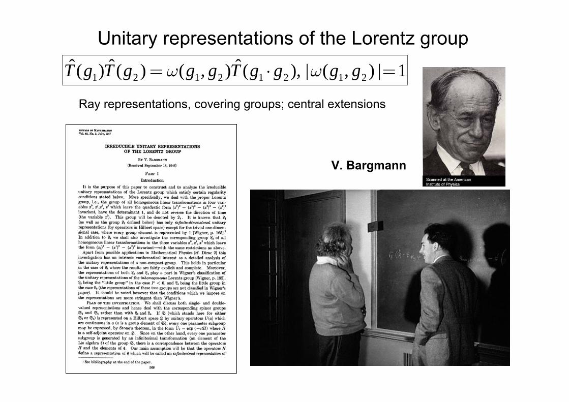
Unitary representations of the Lorentz group

{ }, , 1.

ˆ ˆ ˆ( ) : ,ˆ ˆ

i ie e

g T g T T

T T

θ θ

+

∗+

Ψ Ψ Ψ ⊂Η Ψ =

→ Ψ Φ = Ψ Φ

Ψ Φ = Ψ Φ

∼

1 2 1 2 1 2 1 2ˆ ˆ ˆ( ) ( ) ( , ) ( ), | ( , ) | 1T g T g g g T g g g gω ω= ⋅ =

V. Bargmann

Ray representations, covering groups; central extensions

7

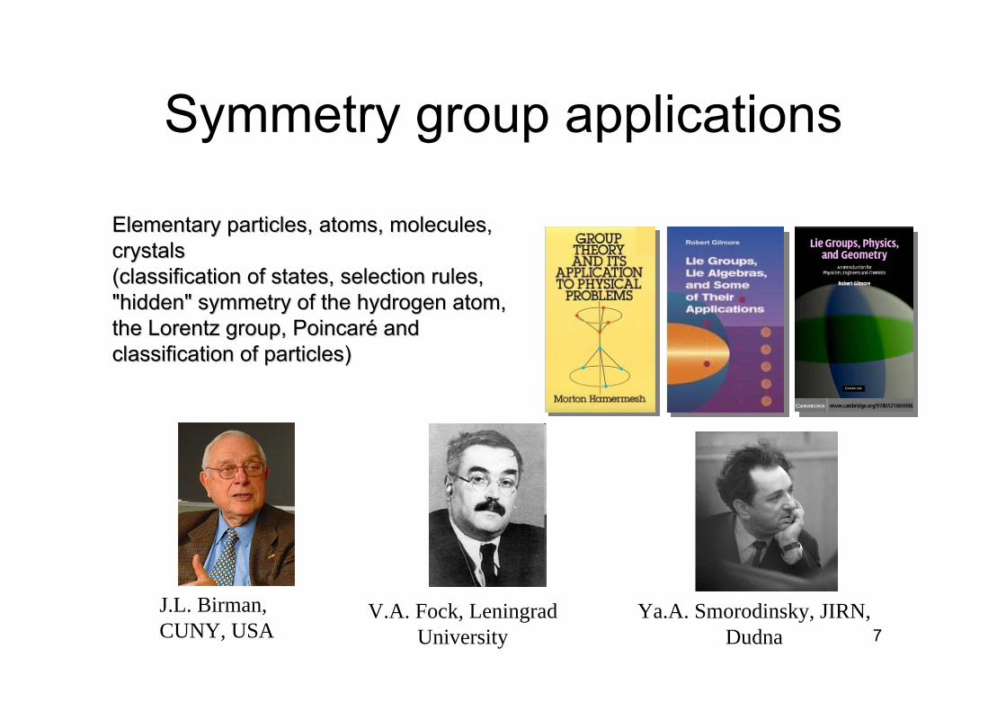
Symmetry group applications

Elementary particles, atoms, molecules, Elementary particles, atoms, molecules, crystals crystals (classification of states, selection rules, (classification of states, selection rules, "hidden" symmetry of the hydrogen atom, "hidden" symmetry of the hydrogen atom, the Lorentz group, Poincarthe Lorentz group, Poincaréé and and classification of particles)classification of particles)

J.L. Birman, CUNY, USA

Ya.A. Smorodinsky, JIRN, Dudna

V.A. Fock, Leningrad University

8

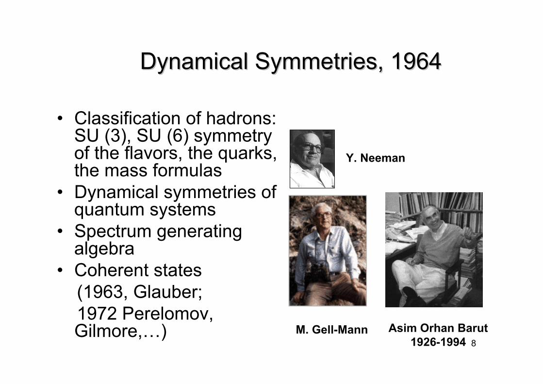
Dynamical Symmetries, 1964Dynamical Symmetries, 1964

• Classification of hadrons: SU (3), SU (6) symmetry of the flavors, the quarks, the mass formulas

• Dynamical symmetries of quantum systems

• Spectrum generating algebra

• Coherent states (1963, Glauber; 1972 Perelomov, Gilmore,…) M. Gell-Mann

Y. Neeman

Asim Orhan Barut 1926-1994

9

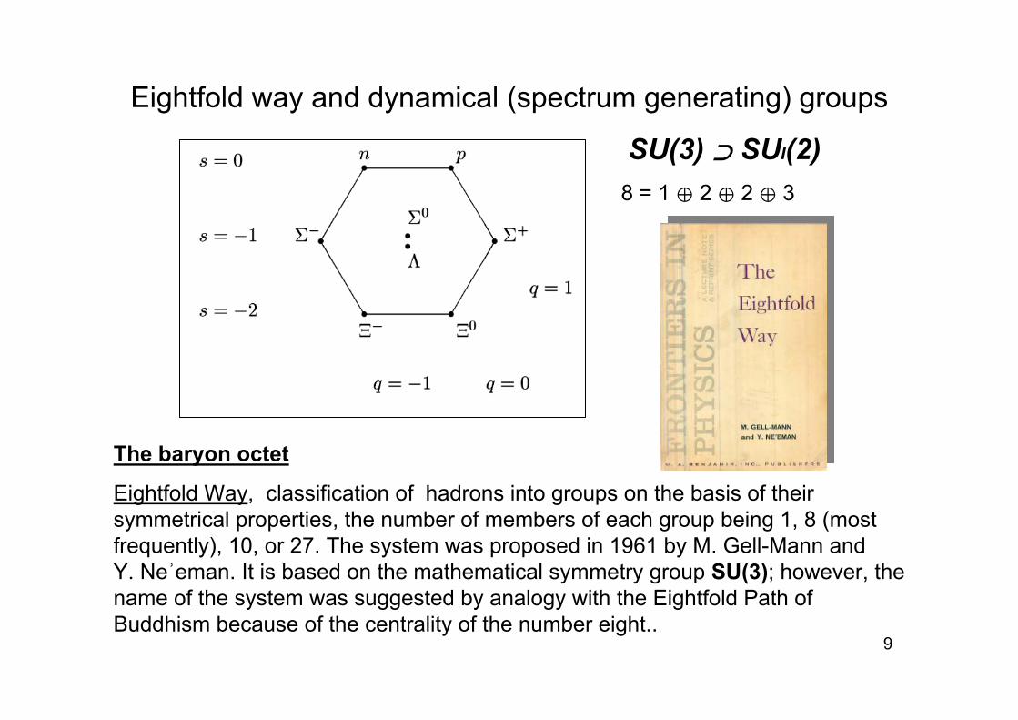
Eightfold way and dynamical (spectrum generating) groups

The baryon octet

Eightfold Way, classification of hadrons into groups on the basis of their symmetrical properties, the number of members of each group being 1, 8 (most frequently), 10, or 27. The system was proposed in 1961 by M. Gell-Mann and Y. Neʾeman. It is based on the mathematical symmetry group SU(3); however, the name of the system was suggested by analogy with the Eightfold Path of Buddhism because of the centrality of the number eight..

SU(3) … SUI(2)8 = 1 ∆ 2 ∆ 2 ∆ 3

10

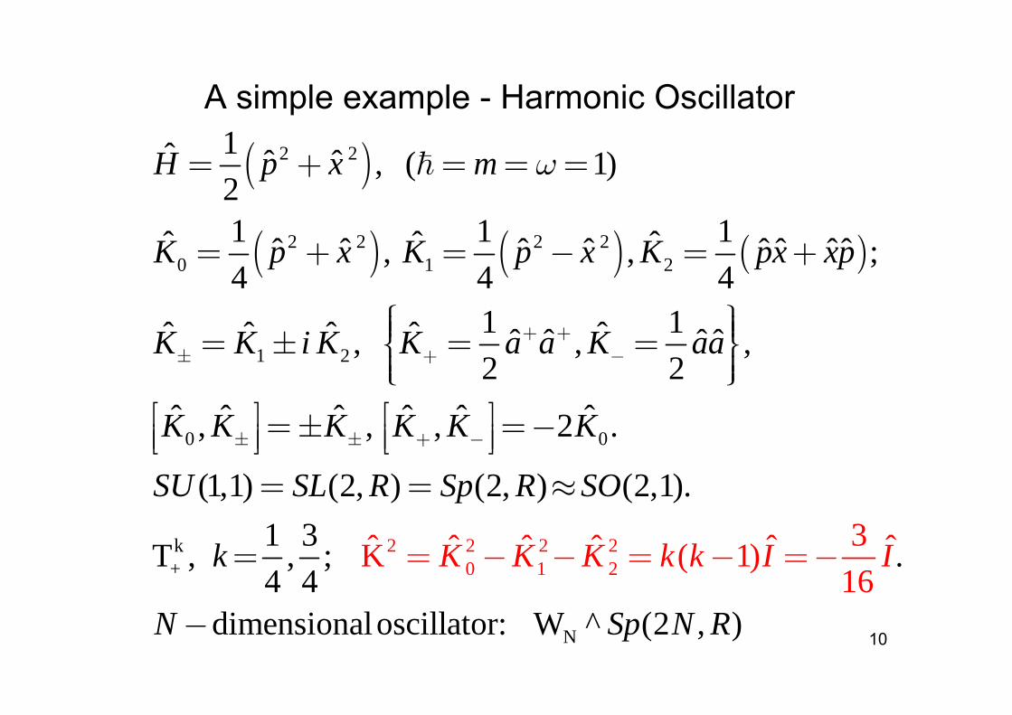
A simple example - Harmonic Oscillator

( )

( ) ( ) ( )

2 2

2 2 2 20 1 2

1 2

0 0

k+

1ˆ ˆ ˆ , ( 1)21 1 1ˆ ˆ ˆˆ ˆ ˆ ˆ ˆ ˆ ˆˆ, , ;4 4 4

1 1ˆ ˆ ˆ ˆ ˆˆ ˆ ˆ ˆ, , ,2 2

ˆ ˆ ˆ ˆ ˆ ˆ, , , 2 .

(1,1) (2, ) (2, ) (2,1).1 3T , , ;4 4

H p x m

K p x K p x K px xp

K K i K K a a K aa

K K K K K K

SU SL R Sp R SO

k

ω

+ +± + −

± ± + −

= + = = =

= + = − = +

⎧ ⎫⎪ ⎪⎪ ⎪= ± = =⎨ ⎬⎪ ⎪⎪ ⎪⎩ ⎭⎡ ⎤ ⎡ ⎤=± =−⎢ ⎥ ⎢ ⎥⎣ ⎦ ⎣ ⎦

= = ≈

= 2 2 2 20 1 2

N

3ˆ ˆ ˆ ˆ ˆ .̂

dimensionaloscill

K ( 1)

ator: W ^1

)6

(2 ,N

K K K

Sp N

k k

R

I I= − − = − =−

−

11

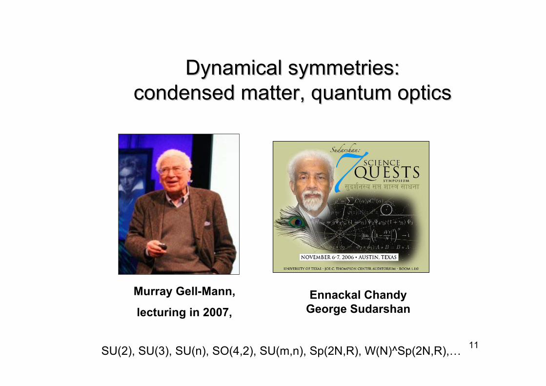
Dynamical symmetries:Dynamical symmetries:condensed mattercondensed matter, , quantum opticsquantum optics

Murray Gell-Mann,

lecturing in 2007,Ennackal Chandy

George Sudarshan

SU(2), SU(3), SU(n), SO(4,2), SU(m,n), Sp(2N,R), W(N)^Sp(2N,R),…

12

13

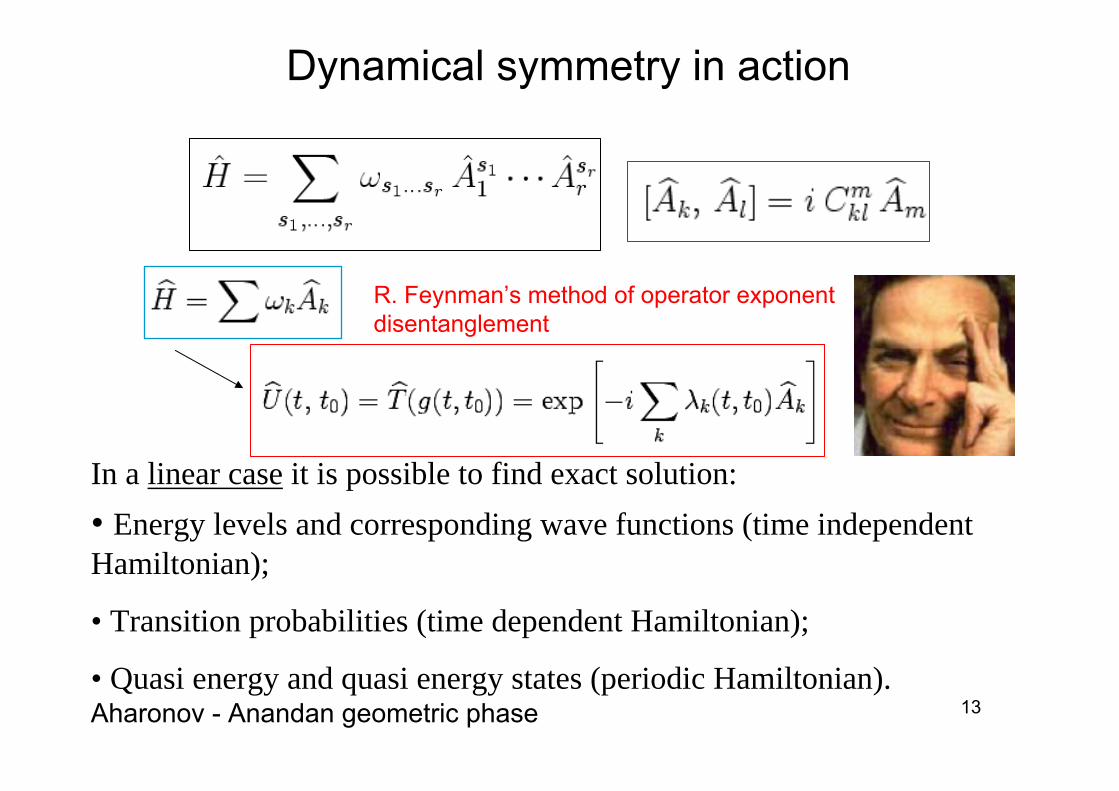
Dynamical symmetry in action

In a linear case it is possible to find exact solution:• Energy levels and corresponding wave functions (time independentHamiltonian);

• Transition probabilities (time dependent Hamiltonian);

• Quasi energy and quasi energy states (periodic Hamiltonian).Aharonov - Anandan geometric phase

R. Feynman’s method of operator exponent disentanglement

14

( )( ) ( ) ( )1 1 2 2 2

ˆ ˆˆ ( ),' "

' "ˆ ...

A,A A A ...,

A A A

k kH f A A

H f C f C f Cα α α

= ∈

⎛ ⎞ ⎛ ⎞= + + +⎜ ⎟ ⎜ ⎟⎝ ⎠ ⎝ ⎠

⊃ ⊃ ⊃

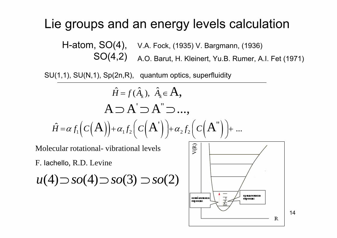
Lie groups and an energy levels calculation

Molecular rotational- vibrational levels

F. Iachello, R.D. Levine

(4) (4) (3) (2)u so so so⊃ ⊃ ⊃

H-atom, SO(4), SO(4,2)

V.A. Fock, (1935) V. Bargmann, (1936)

A.O. Barut, H. Kleinert, Yu.B. Rumer, A.I. Fet (1971)

SU(1,1), SU(N,1), Sp(2n,R), quantum optics, superfluidity

15

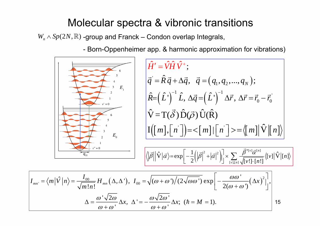
Molecular spectra & vibronic transitions(2 , )nW Sp N∧ R

( )

( ) ( )

[ ]( ) [ ] [ ] [ ]

'1 2

1 1 '0 0

' '

;ˆ , , ,..., ;

ˆ ˆ ˆ ˆ' , ' ,

, |

ˆ ˆ ˆ ˆ

ˆ ˆ ˆ ˆV =T( )D( ) U(R)ˆI V

Nq R q q q q q q

R L L q

H

L r r r r

m n

VH

m n m n

V

δ ρ

− −

+

= +Δ =

= Δ = Δ Δ = −

⎡ ⎤ ⎡ ⎤=⎣ ⎦ ⎣ ⎦

′ =

< >=

( ) *[ ] [ ]2 2

[ ],[ ]

1exp [ ] [ ]2 [ !] [ !]

ˆ ˆV Vv n

v nv n

v nβ αβ α β α⎡ ⎤= − + ×⎢ ⎥ ⋅⎣ ⎦

∑

-group and Franck – Condon overlap Integrals,

- Born-Oppenheimer app. & harmonic approximation for vibrations)

( ) ( )200' 00

'ˆ , ' , ( ') (2 ') exp ,2( ')! !

' 2 2 ', ' ; ( 1).' '

mn mnII m V n H I xm n

x x M

ωωω ω ωωω ω

ω ω ω ωω ω ω ω

⎡ ⎤= = Δ Δ = + − Δ⎢ ⎥+⎣ ⎦

Δ = Δ Δ = − Δ = =+ +

16

17

Model Hamiltonians, dynamical groups and coherent states

Klauder, Glauber, Sudarshan, Perelomov, Berezin, Gilmore, …

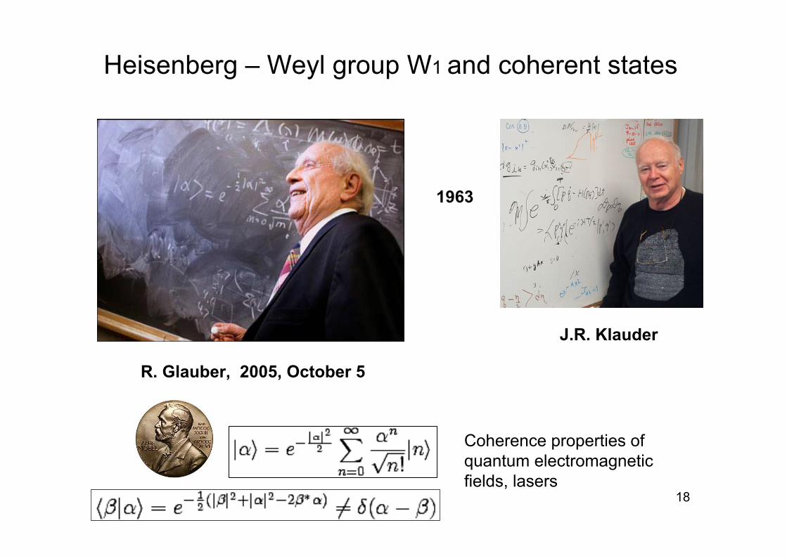
18

J.R. Klauder

R. Glauber, 2005, October 5

Heisenberg – Weyl group W1 and coherent states

Coherence properties of quantum electromagnetic fields, lasers

1963

19

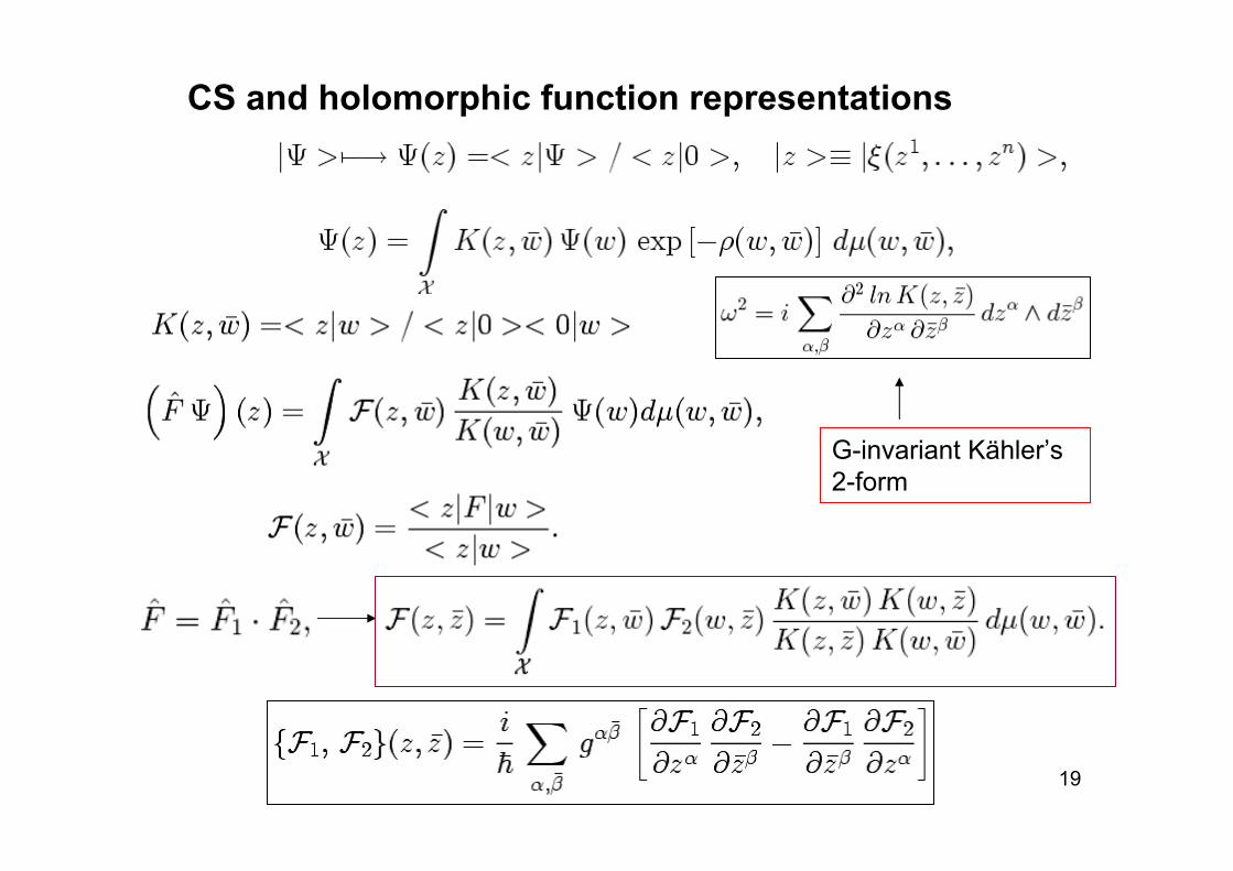
CS and holomorphic function representations

G-invariant Kähler’s 2-form

20

Path Integrals in CS - representation

0 0 1 1 2 1 0ˆ ˆ ˆ ˆ ˆ( , ) ( , ) ( , ) ( , ) ( , )N N N N NU t t U t t U t t U t t U t t− − −≡ = ⋅⋅⋅

21

“Classical” Equations

2

1

2

1

( , ) ln ( , ) ,

( , ) ln ( , ) .

n

n

i z z K z z zz z z

i z z K z z zz z z

βα α β

β

βα α β

β

=

=

∂ ∂=

∂ ∂ ∂

∂ ∂− =

∂ ∂ ∂

∑

∑

2 ln ( , ) , , .K z zg g g g gz z

α β α α β βκ αγ γαβ κβα β δ δ∂

= ⋅ = ⋅ =∂ ∂

For linear systems classical dynamics of coherent states is exact!

22

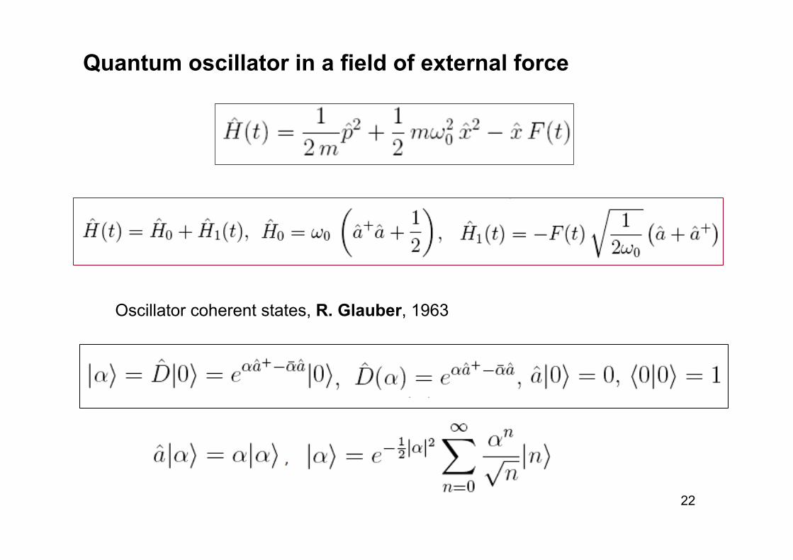
Quantum oscillator in a field of external force

Oscillator coherent states, R. Glauber, 1963

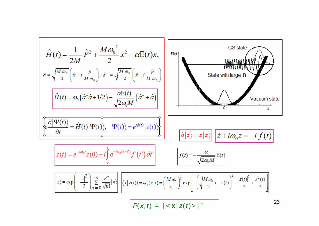
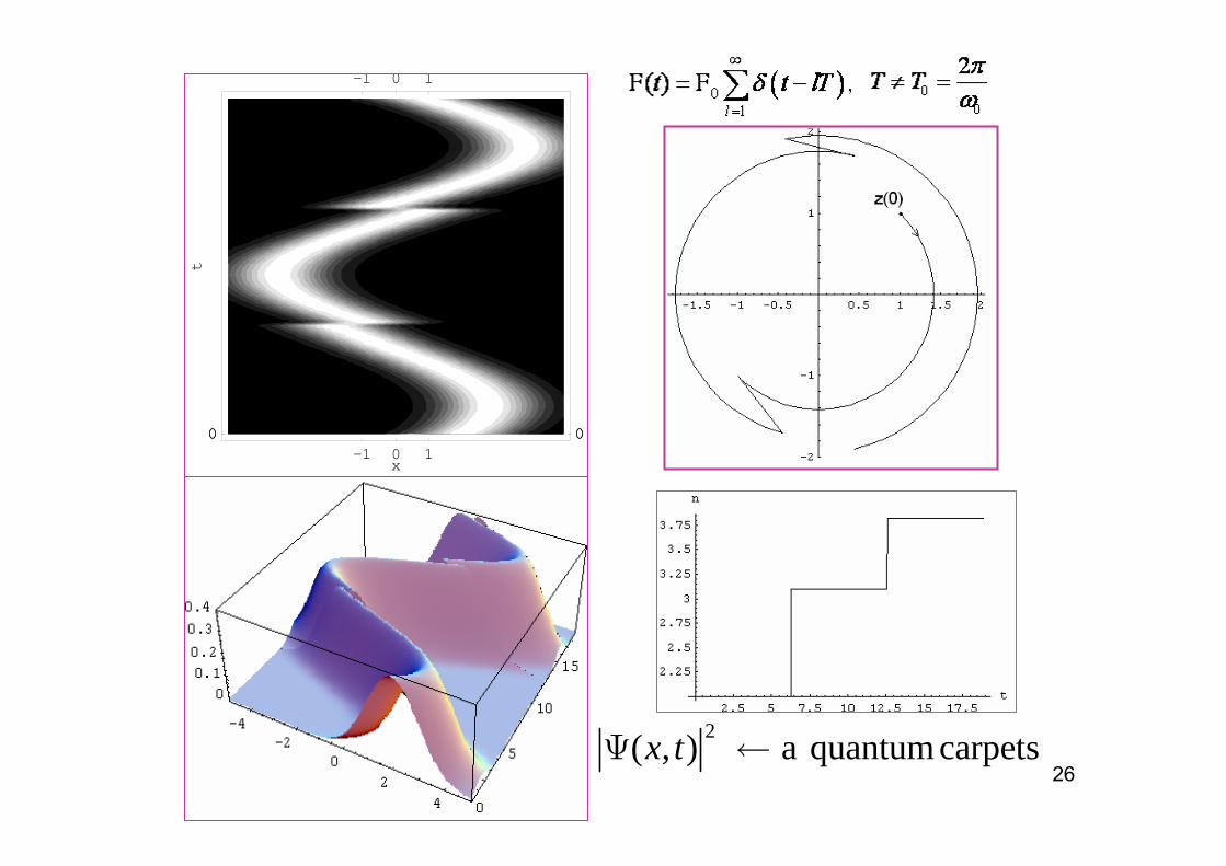
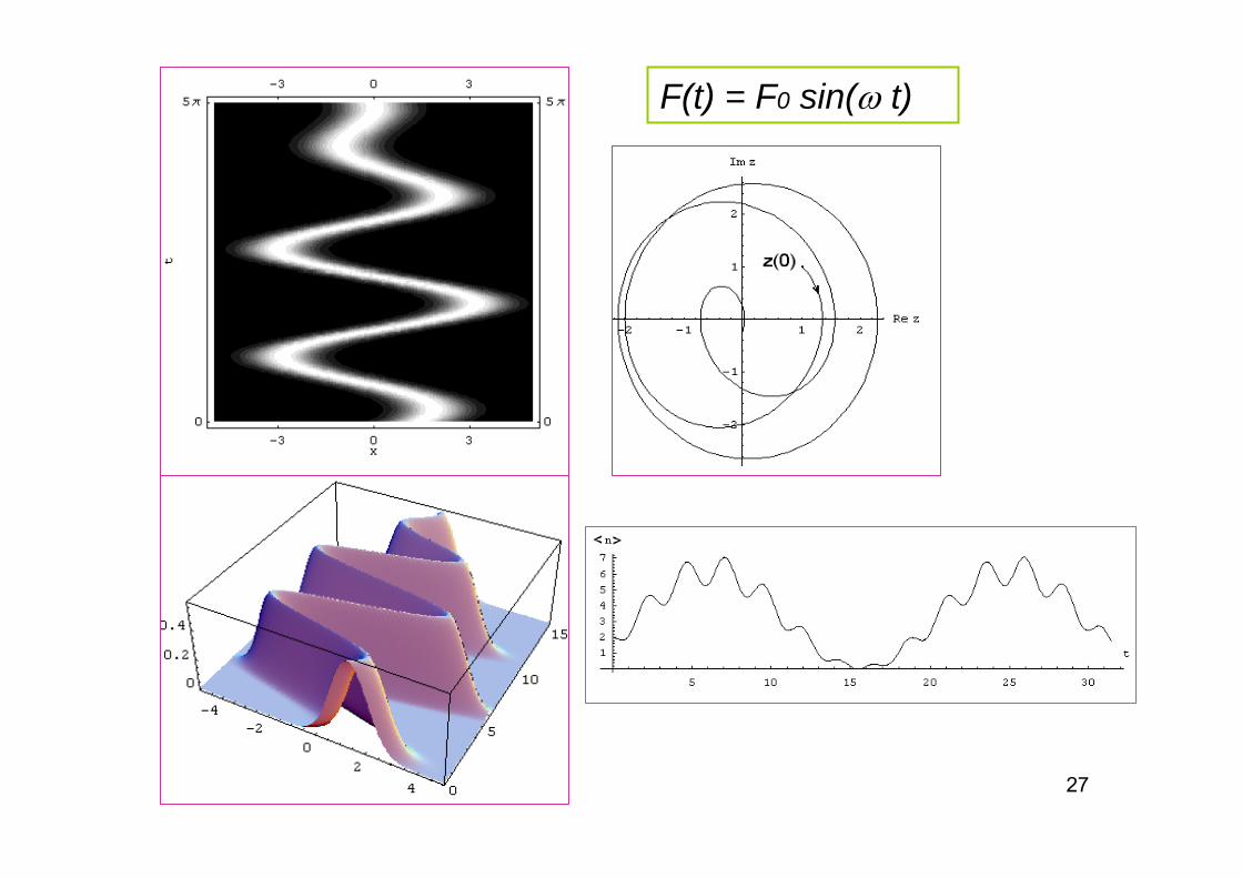
23P(x,t) = |<x|z(t)>|2

24

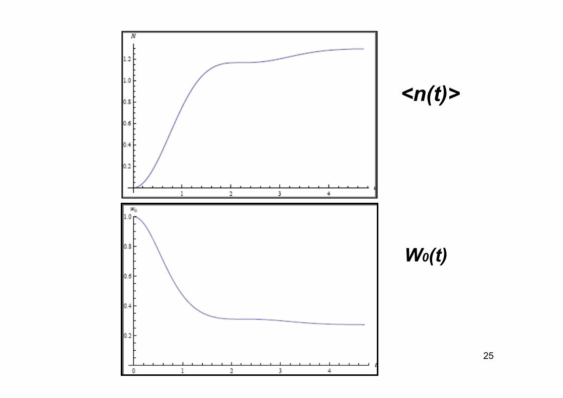
25

<n(t)>

W0(t)

26

0-1 1x

00

t

0-1 1

00

2( , ) a quantum carpetsx tΨ ←

27

F(t) = F0 sin(ω t)

28

N-level atoms in classical fields. G = SU(N), ( |k><l| œ u(N) )

29

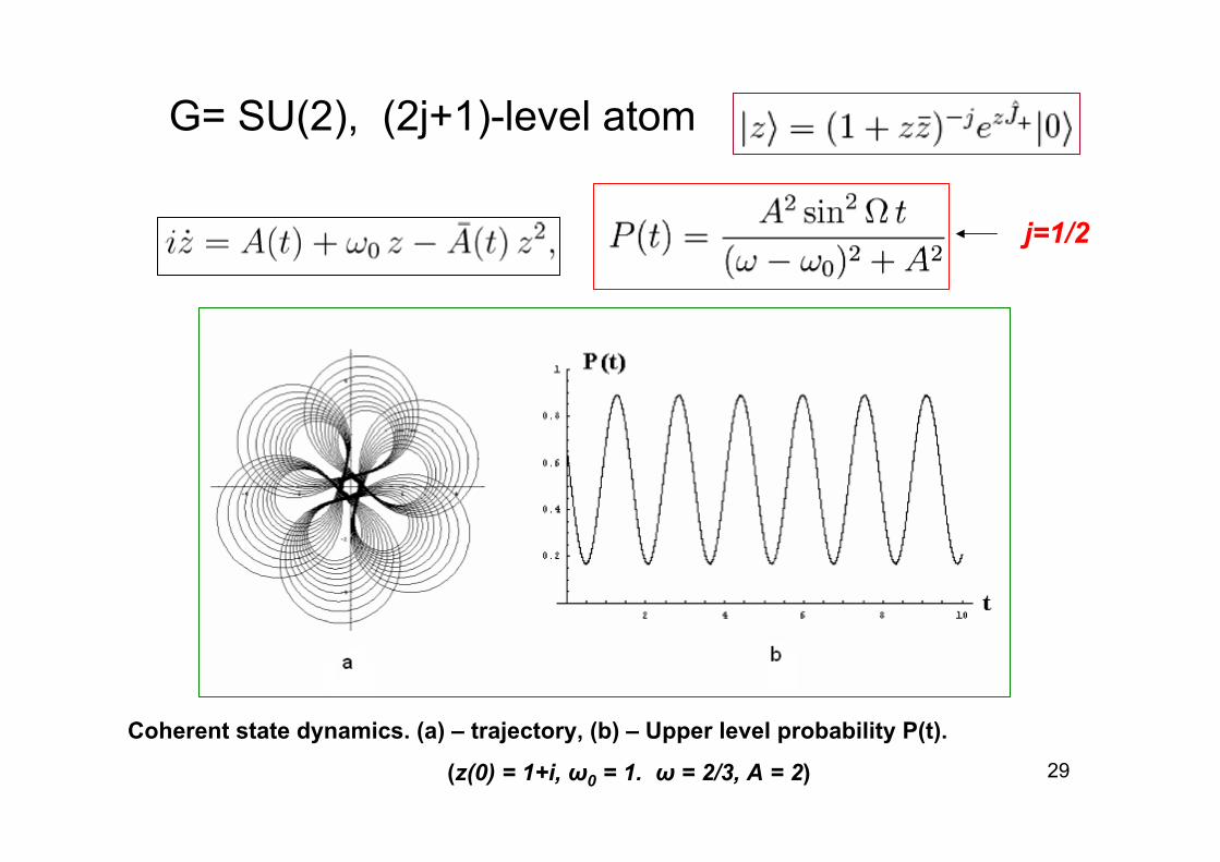
G= SU(2), (2j+1)-level atom

Coherent state dynamics. (a) – trajectory, (b) – Upper level probability P(t).

(z(0) = 1+i, ω0 = 1. ω = 2/3, A = 2)

j=1/2

30

Complex plane & Bloch’s sphere

tan2

iz e φ ϑ⎛ ⎞= ⎜ ⎟⎝ ⎠

31

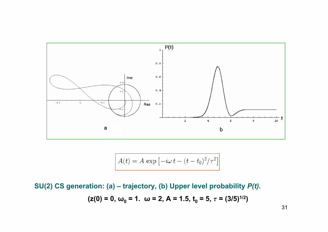
SU(2) CS generation: (a) – trajectory, (b) Upper level probability P(t).

(z(0) = 0, ω0 = 1. ω = 2, A = 1.5, t0 = 5, t = (3/5)1/2)

32

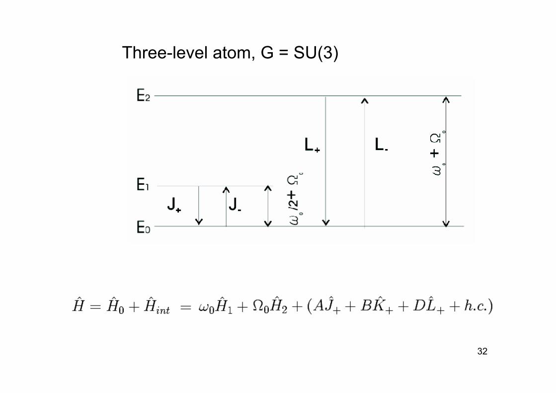
Three-level atom, G = SU(3)

33Case of V – atom transitions and dynamics of the level populations.

We have not here a funny pictures for CS trajectories as in SU(2) case…

coherent population trapping

34

Molecular rotator in external magnetic field

A symbol of the hamiltonian:

( ) ( )2

2 23

1 2 1 2 3

22 22 31 2

1 2 3

2 2 21 1 1 1ˆ ˆ ˆ ˆ ˆ ˆ ˆ8 8 8 8 2

ˆˆ ˆˆ ˆ( ) ( )2 2 2

ˆ( ) ,J J J J J J JI I I I I

JJ JH t V tI I I

B t Jγ+ − + − − +− + + + +

⎛ ⎞= + + + =⎜ ⎟

⎝ ⎠⎛ ⎞ ⎛ ⎞

= + −⎜ ⎟ ⎜ ⎟⎝ ⎠ ⎝ ⎠

2 2 2 2 2 2

2 2 2

ˆ( , , ) ( )

4 2 1 (1 ) / 2 (1 )2 (2 1)(1 ) (1 ) (1 )

( ) .1

i t i t

z z t z H t z

z z Jzz Jz z J z z J zzJ a J b czz zz zz

ze zeJB tzz

ω ω

γ−

= =

⎧ ⎫⎛ ⎞+ + + + + −⎪ ⎪= − + + −⎨ ⎬⎜ ⎟+ + +⎪ ⎪⎝ ⎠⎩ ⎭+

−+

2 1 2 1

1 2 1 2 3

1, , .8 8 2I I I Ia b c

I I I I I− +

= = =

( )1 2( ) ( ) cos sin .B t B t e t e tω ω= +

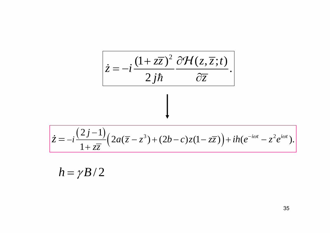
35

( ) ( )3 22 12 ( ) (2 ) (1 ) ( ).

1i t i ti

ja z z b c z zz ih e z e

zzz ω ω−−

−− + − − + −

+=

2(1 ) ( , ; ) .2

zz z z tz ij z

+ ∂= −

∂

/ 2h Bγ=

3636

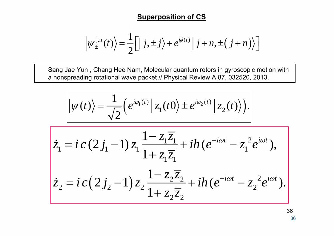
Superposition of CS

( )1 2( ) ( )1 2

1( ) ( 0 ( ) .2

i t i tt e z t e z tϕ ϕψ = ±

( )

21 11 1 1 1

1 1

22 22 2 2 2

2 2

1(2 1) ( ),112 1 ( ).1

i t i t

i t i t

z zz i c j z ih e z ez zz zz i c j z ih e z ez z

ω ω

ω ω

−

−

−= − + −

+−

= − + −+

( )j,n ( )1( ) , ,2

i tt j j e j n j nφψ ± ⎡ ⎤= ± + + ± +⎣ ⎦

Sang Jae Yun , Chang Hee Nam, Molecular quantum rotors in gyroscopic motion witha nonspreading rotational wave packet // Physical Review A 87, 032520, 2013.

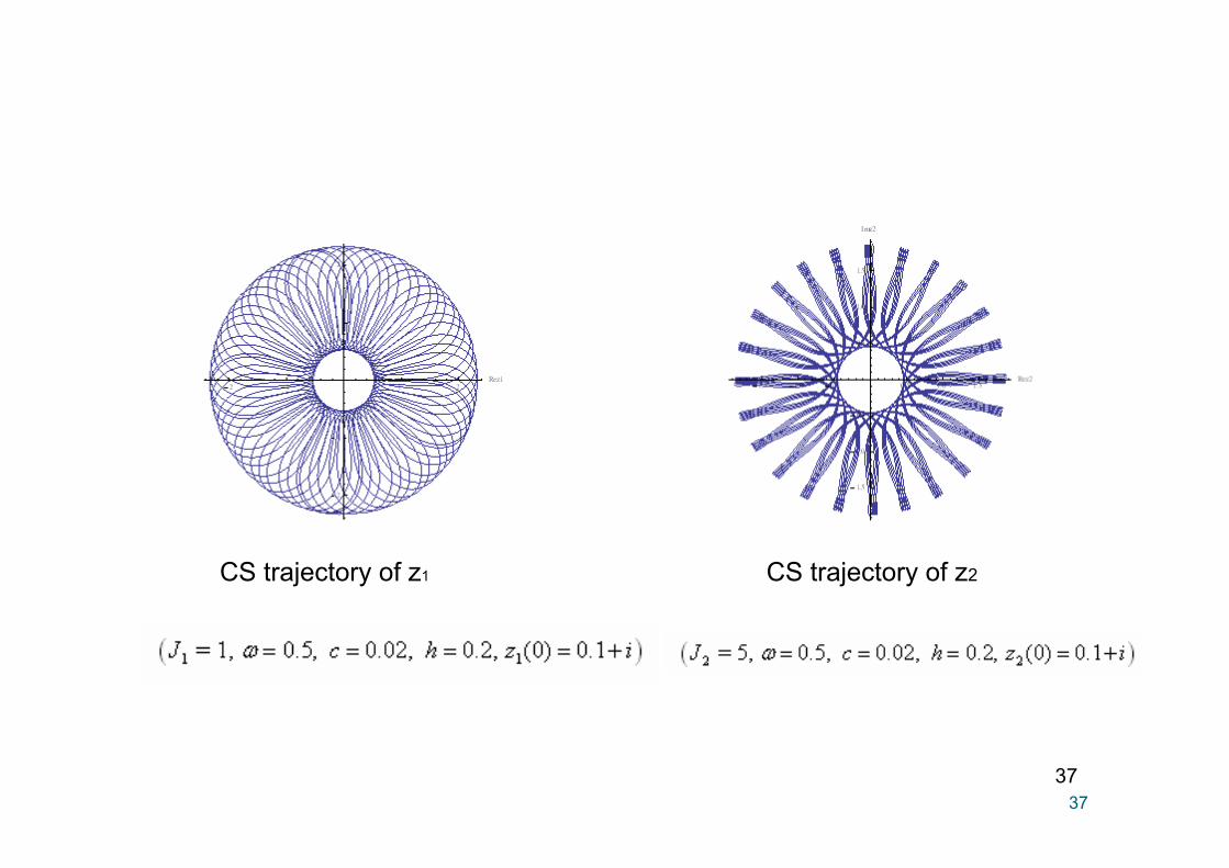
3737

CS trajectory of z1 CS trajectory of z2

38

39

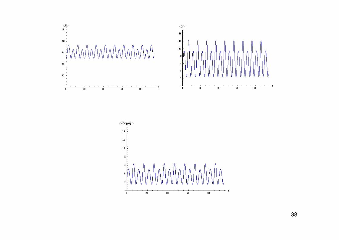
Dynamical chaos of CS parameters for two-level models

ω0ω

1 (2),G W SU CS α ζ= ⊗ = ⊗/ 2; 1,2,...j N N= =

( 1)N àThe Dicke model

m =1, 2.

One-atom maser j = 1/2

40

“Bee-like” trajectory for atomic SU(2)

g=λ=0.2; ν=1.1, ω=1. J = 1

41

Mean values and chaos

42

43

The Dicke – model with parametric interaction

(1) (2)

44

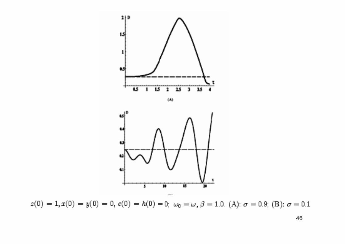
Lyapunov’s maximal coefficient

45

46

47

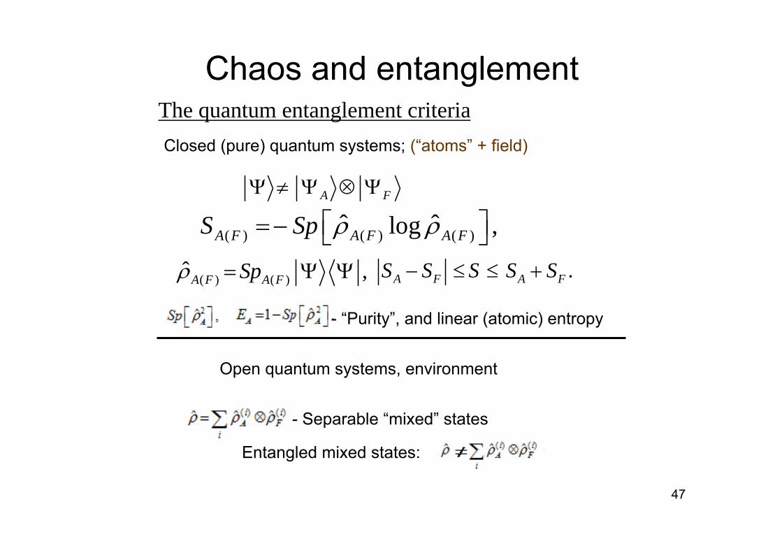
Chaos and entanglement

A FΨ ≠ Ψ ⊗ Ψ

The quantum entanglement criteria

( ) ( ) ( )ˆ ˆlog ,A F A F A FS Sp ρ ρ⎡ ⎤=− ⎣ ⎦

( ) ( )ˆ ,A F A FSpρ = Ψ Ψ .A F A FS S S S S− ≤ ≤ +

- “Purity”, and linear (atomic) entropy

Closed (pure) quantum systems; (“atoms” + field)

- Separable “mixed” states

Entangled mixed states:

Open quantum systems, environment

48

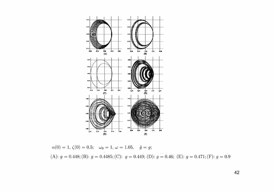
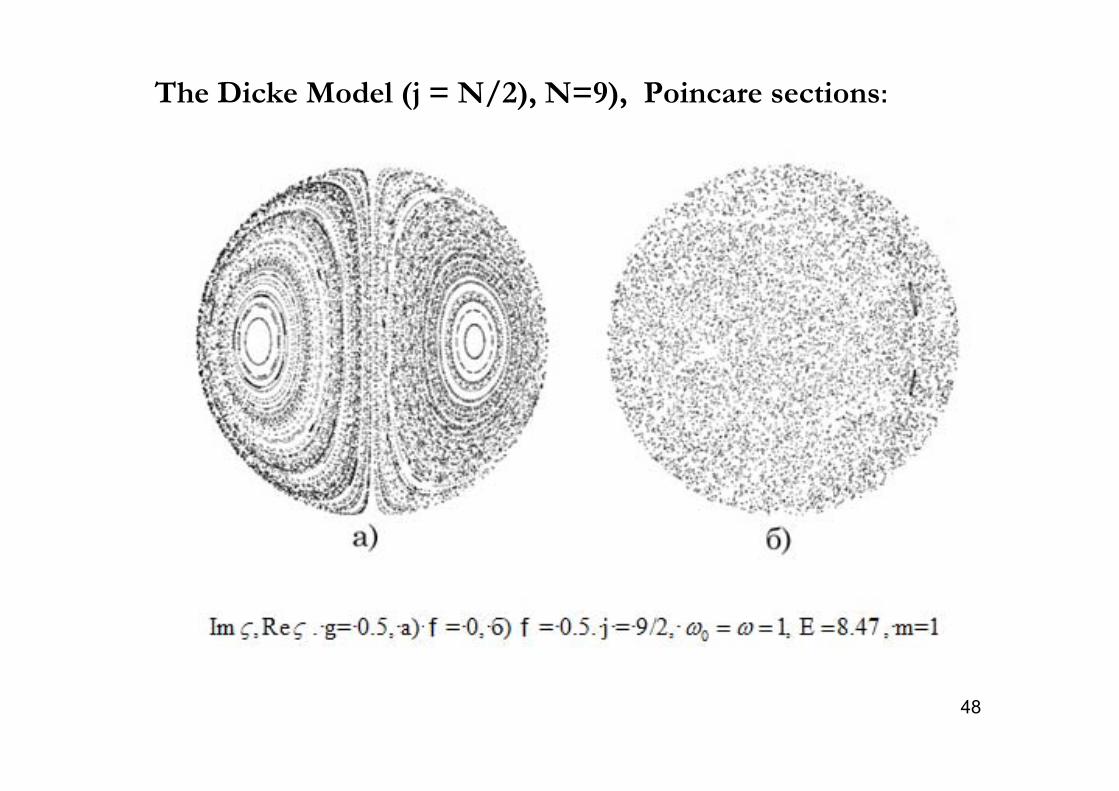
The Dicke Model (j = N/2), N=9), Poincare sections:

49

20 0( ) ( ) ( , ; , | ) , .t d d f tα μ ς α ζ α ζ α ζΕΨ = ∫∫

( )2

22

Re Im 2 1 Re Im, ( ) .1 | |

d d j d dd dα α ς ςα μ ςπ π ς

+= =

+

0 0 2 0 2 00lim ( , | , ; ) ( ) ( )t

f tα ζ α ζ δ α α δ ζ ζΕ→= − −

2ˆ( ) 1 ( ) ,A F AE t Sp tρ⎡ ⎤= − ⎣ ⎦ { }max max ( ) ,AtE E t= ( )

01 ( ) .

T

A AE T E t dt= ⋅ ∫

We have to calculate:

2( ; ) ( ); ( ; ) exp ( ) ( ) ; ( ) ,j

j jE m m m m cl m

m j

f f t f t t t j mα ψ ζ α κ α α ψ ζ ζ=−

⎡ ⎤= ∼ − ⋅ − =⎣ ⎦∑

( )( )

ˆ ˆ| | ; | 2 | ;

ˆ ˆ | 2 | .

a a

a a

α α α α α α α

α α α αα α

+

+

>= > >= ∂ ∂ + >

>= ⋅∂ ∂ + >

( ) ( )( )

2

0 2

ˆ ˆ| (1 ) | ; | (1 ) | ;

ˆ | (1 ) (1 ) | .j

J j J j

J

ζ ζ ζ ζζ ζ ζ ζ ζ ζ ζζ ζ

ζ ζ ζ ζζ ζζ ζ

+ −>= ∂ ∂ + + > >= − ⋅∂ ∂ + + >

>= ⋅∂ ∂ + − + >

The initial condition:

(0) (0) (0) .α ζΨ = | > ⊗ | > ˆ ˆ(0) (0) ( ) ( ) ;E H t H tΕ = = Ψ Ψ = Ψ Ψ

ˆ( ) ( )i t H tt∂

Ψ = Ψ∂

Q-corrections

50

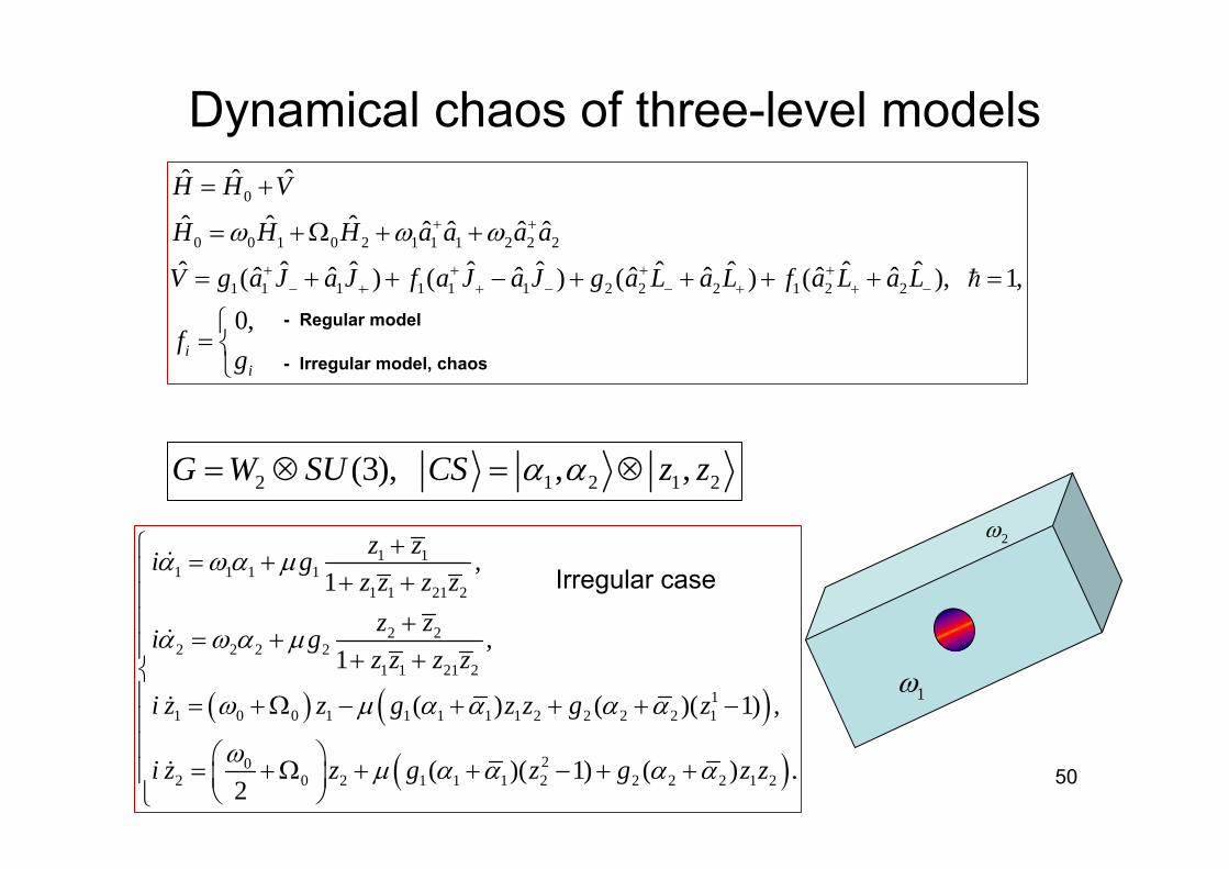
Dynamical chaos of three-level models0

0 0 1 0 2 1 1 1 2 2 2

1 1 1 1 1 1 2 2 2 1 2 2

ˆ ˆ ˆ

ˆ ˆ ˆ ˆ ˆ ˆ ˆˆ ˆ ˆ ˆ ˆ ˆ ˆ ˆ ˆˆ ˆ ˆ ˆ ˆ ˆ ˆ( ) ( ) ( ) ( ), 1,

0,i

i

H H V

H H H a a a a

V g a J a J f a J a J g a L a L f a L a L

fg

ω ω ω+ +

+ + + +− +− + − − + + −

= +

= +Ω + +

= + + − + + + + =

⎧= ⎨⎩

2 1 2 1 2(3), , ,G W SU CS z zα α= ⊗ = ⊗

( ) ( )

( )

1 11 1 1 1

1 1 21 2

2 22 2 2 2

1 1 21 2

11 0 0 1 1 1 1 1 2 2 2 2 1

202 0 2 1 1 1 2 2 2 2 1 2

,1

,1

( ) ( )( 1) ,

( )( 1) ( ) .2

z zi gz z z z

z zi gz z z z

i z z g z z g z

i z z g z g z z

α ωα μ

α ω α μ

ω μ α α α α

ω μ α α α α

+⎧ = +⎪ + +⎪+⎪

= +⎪ + +⎨⎪ = +Ω − + + + −⎪⎪ ⎛ ⎞= +Ω + + − + +⎪ ⎜ ⎟

⎝ ⎠⎩

- Regular model

- Irregular model, chaos

1ω

2ω

Irregular case

51

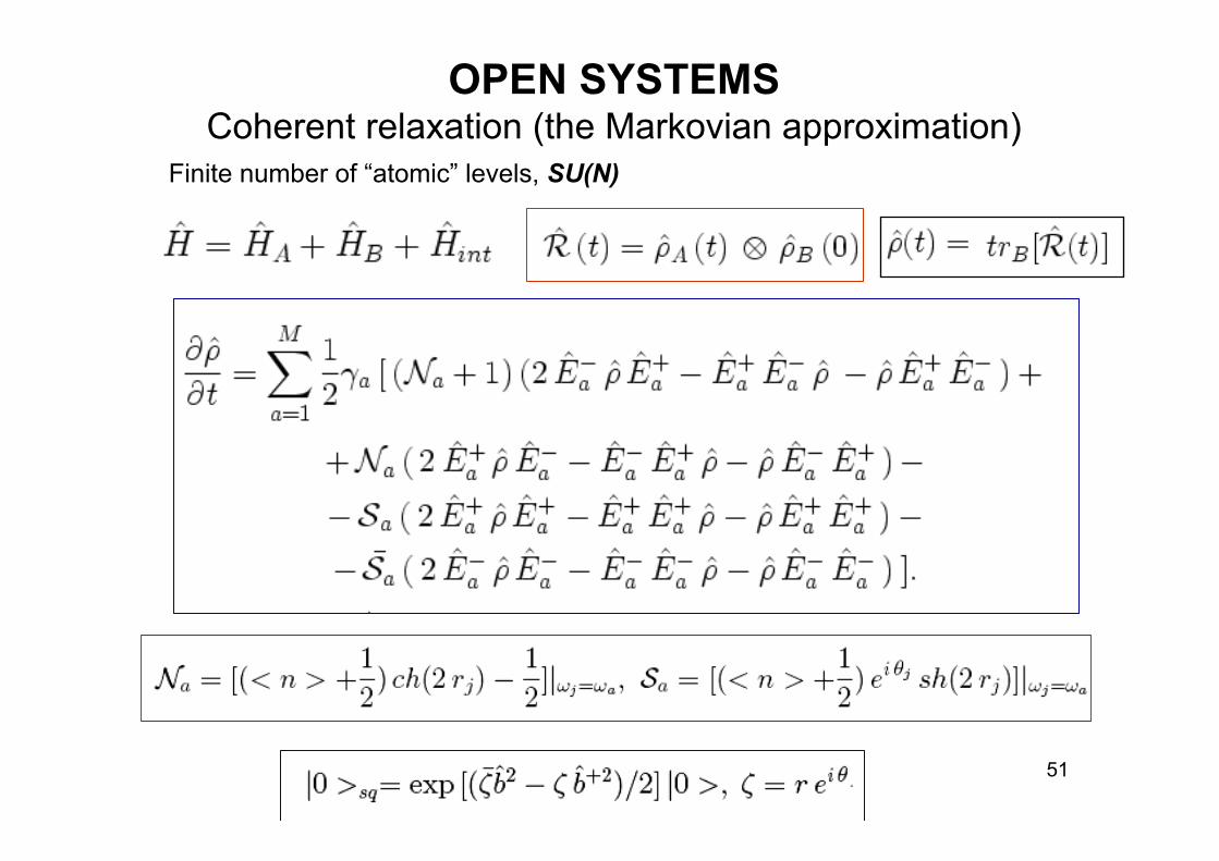
OPEN SYSTEMSCoherent relaxation (the Markovian approximation)

Finite number of “atomic” levels, SU(N)

52

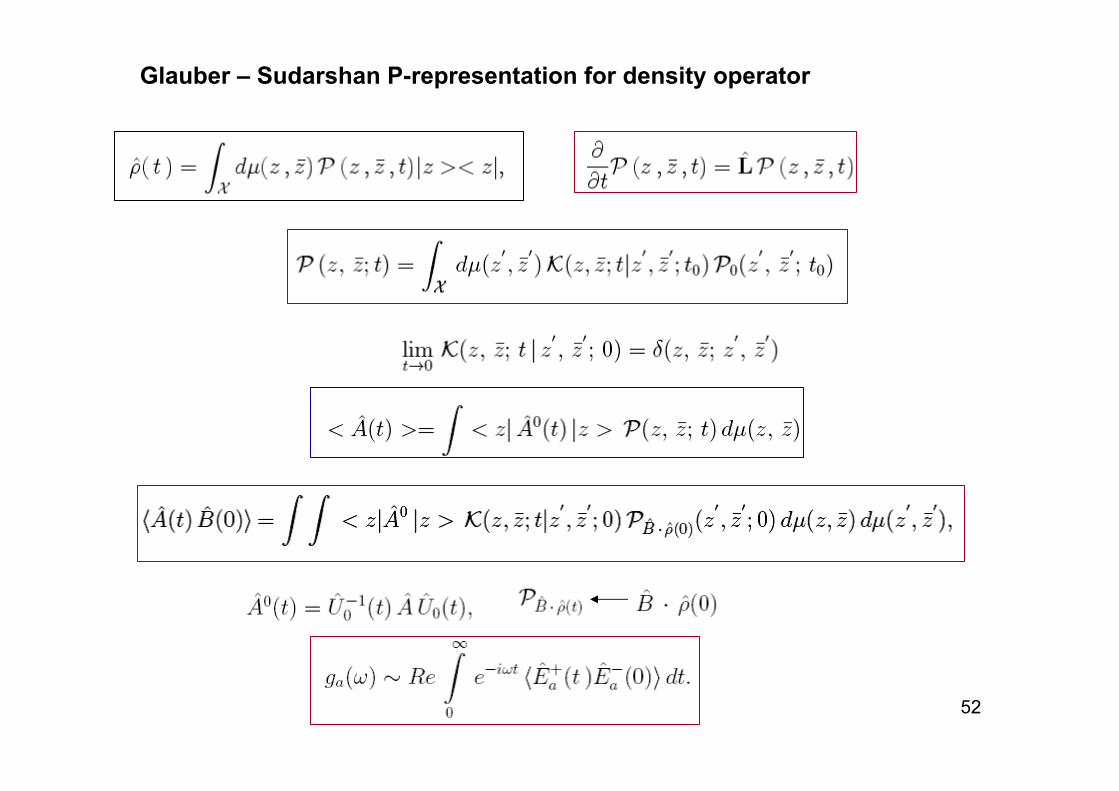
Glauber – Sudarshan P-representation for density operator

53

G=SU(2), (2j+1)-level atom ( j=1/2, 1; j •)

The Fokker-Planck (FP) equation:

54

Method on spherical functions expansion:

FP-equation in the case of squeezed bath:

55

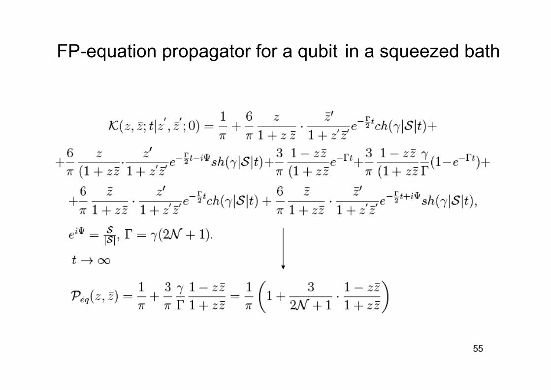
FP-equation propagator for a qubit in a squeezed bath

56

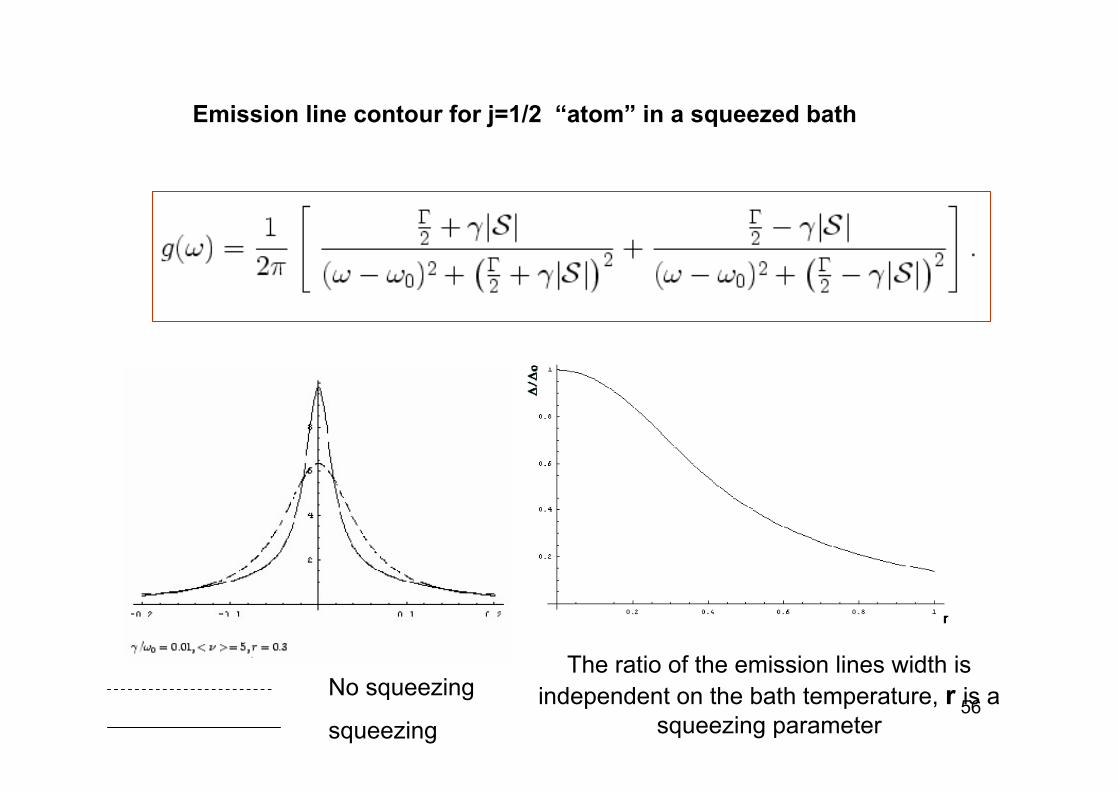
Emission line contour for j=1/2 “atom” in a squeezed bath

No squeezing

squeezing

The ratio of the emission lines width is independent on the bath temperature, r is a

squeezing parameter

57

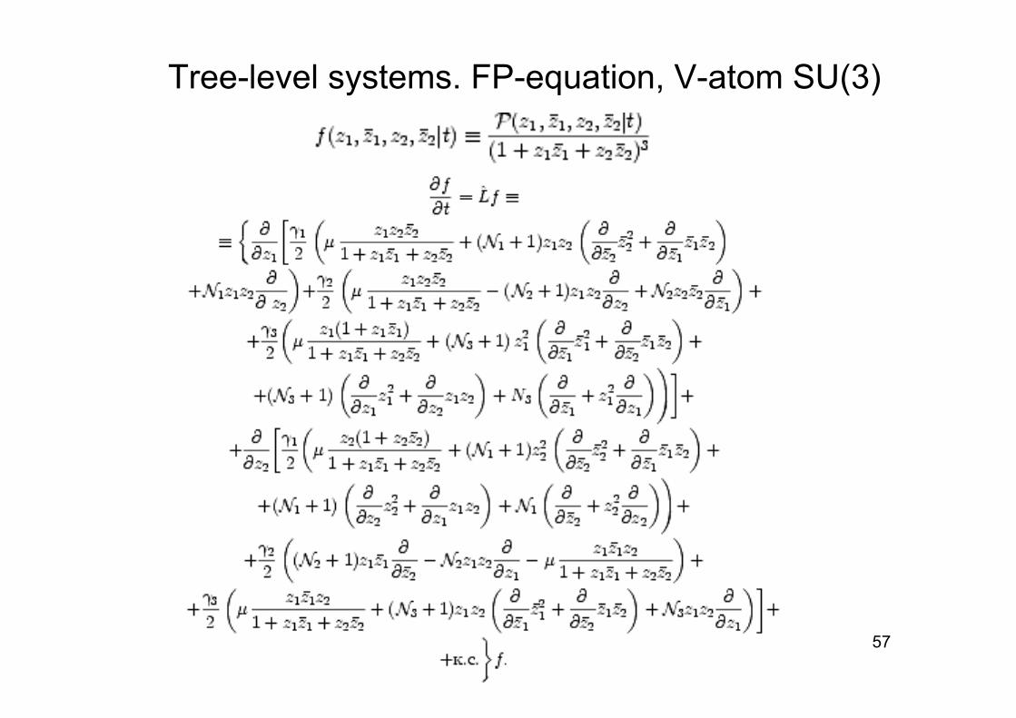
Tree-level systems. FP-equation, V-atom SU(3)

58

Spherical functions on SU(3)/U(2)

1 2 1 2

1 2

1 2 1 2

2

2 2 21 2

( )Y ,

Y ( 3)Y .ˆ, , ,

nl l m nl l mnl l m

nl l m nl l m

f F t

n n

M

=

∇ = +

∇ ∇ ∇

∑

59

Coherent relaxation of large number of “atoms”

60

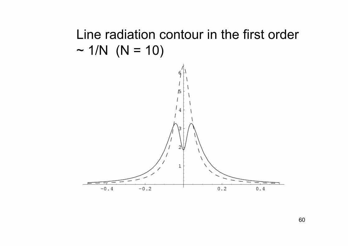
Line radiation contour in the first order~ 1/N (N = 10)

61

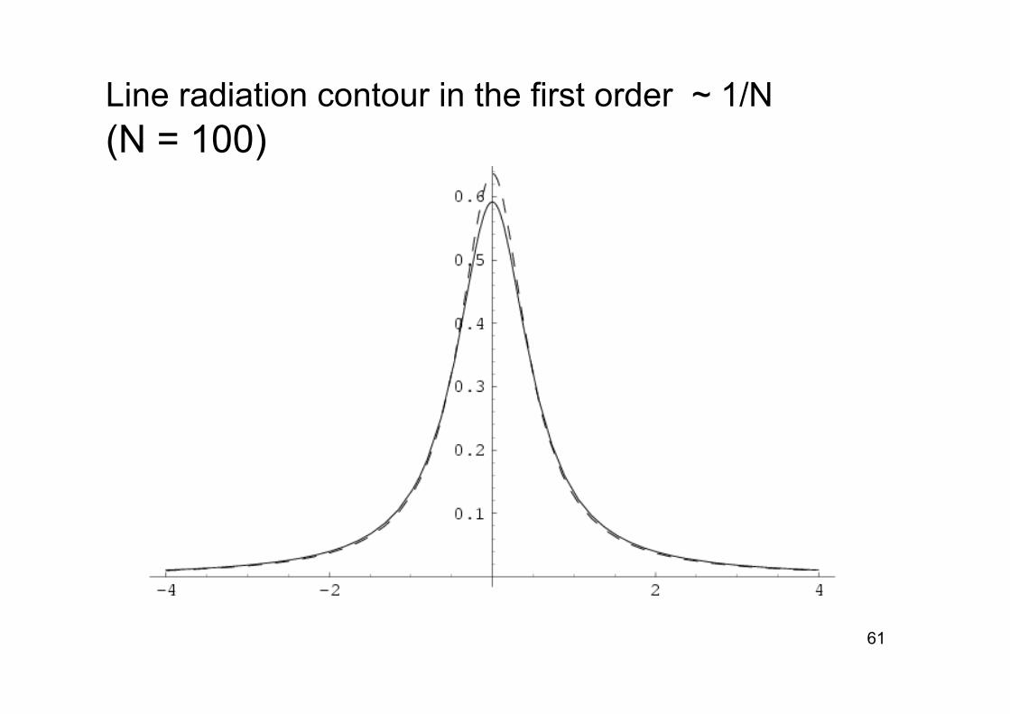
Line radiation contour in the first order ~ 1/N(N = 100)

62

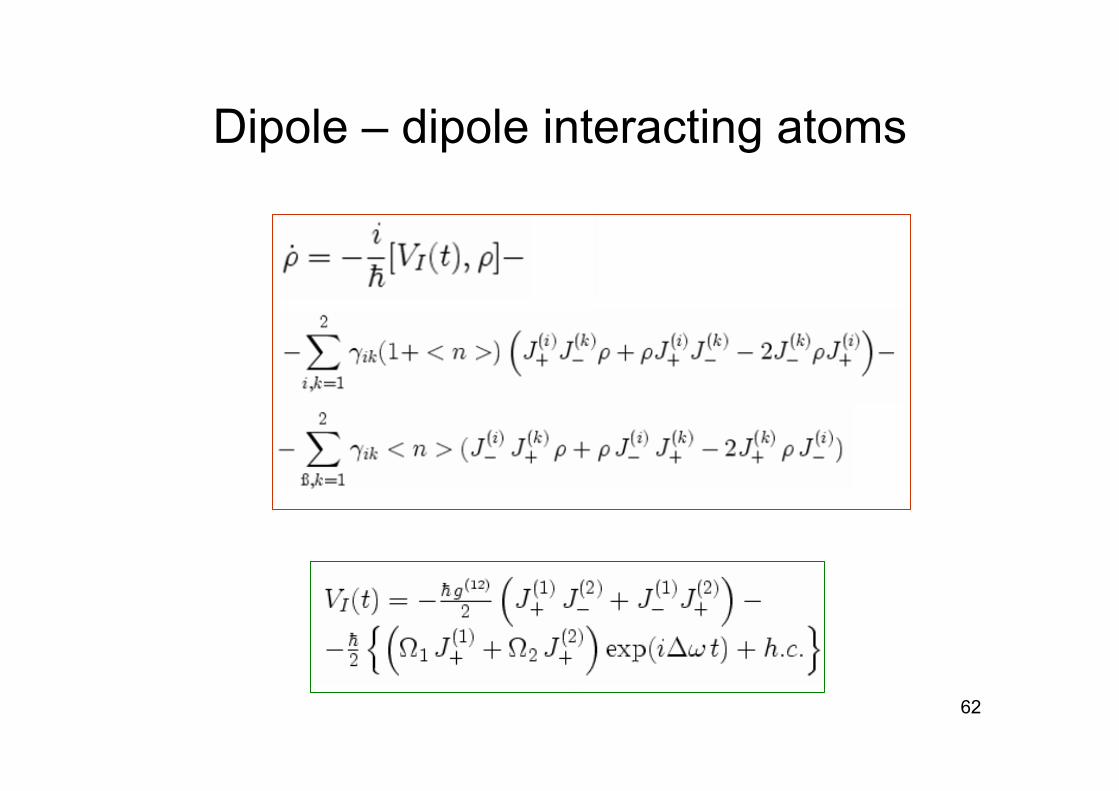
Dipole – dipole interacting atoms

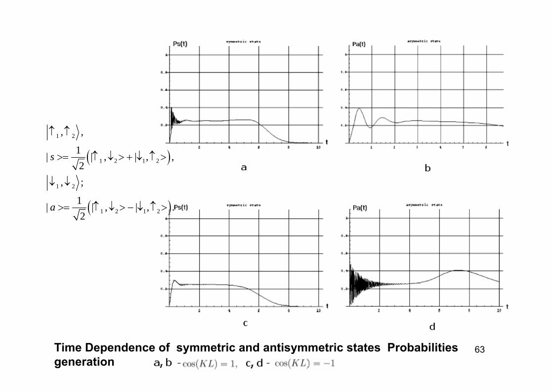
63Time Dependence of symmetric and antisymmetric states Probabilities generation

( )

( )

1 2

1 2 1 2

1 2

1 2 1 2

, ,

1| | , | , ,2

, ;

1| | , | , .2

s

a

↑ ↑

>= ↑ ↓ > + ↓ ↑ >

↓ ↓

>= ↑ ↓ > − ↓ ↑ >

64

Two - level system in external stochastic fields

0 1( )1 1 1 1

0 0

( ) ( ) ( ) , ( ) ( ) ( )t t

i t tK t t t dt K t t t e dtως ς ς −

Ω = Ω Ω =∫ ∫

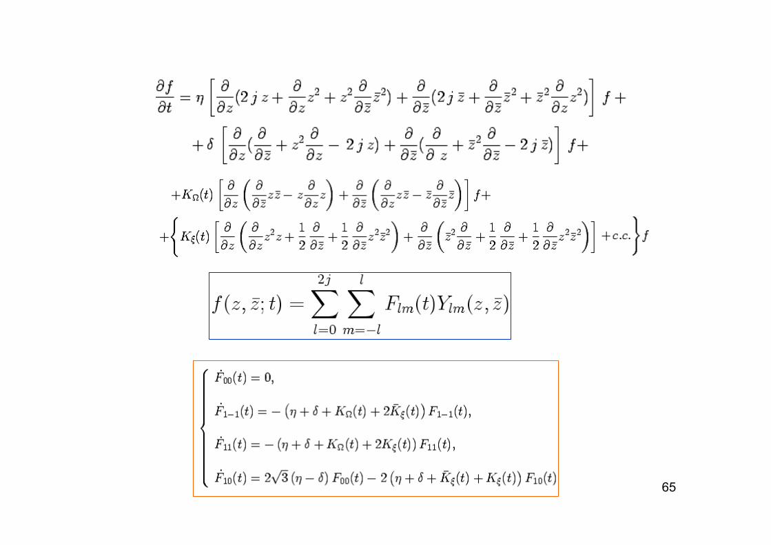
65

66

Probability to find atom in the upper level P↑ for Kubo – Andersen processes

Exact soluble modelPerturbation theoryRelaxation without stochastic field

67

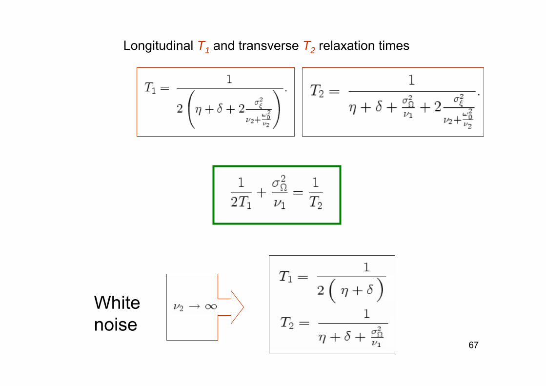
Longitudinal T1 and transverse T2 relaxation times

White noise

68

Line Radiation Contour for Dichotomic Process

(strong field)

Line contour without stochastic field

69

Parametric Amplifier in a thermal squeezed bath2 2

01ˆ ˆ ˆ ˆ ˆ ˆ ˆ( ) ( ) ( )2

i t i tH t a a g aae a a e+ + + −= + + +ω ωω1 1ˆ ˆ ˆ ˆ ˆU ( , ) exp2 2I t t t a a aaξ ξ+ +⎛ ⎞

⎜ ⎟⎝ ⎠

+Δ ≈ −02 exp[ 2 ( ) ]ig t i tξ ω ω= − Δ − −

( ) ( ) ( )0 0ˆ ,P t U t t P t=

( ) ( )00

ˆ , ˆ ˆ ˆ ˆ, , .U t t

LU U t t It

∂= =

∂

( ) ( )

0 02 ( ) t 2 ( ) t

0 02 2

2

2 , 2 ,

2 , 2 ,12 ,2

1 .2

d d d d

d d d d

i id d d d

i t i tr r

r ae r

ge ge

a ad be ge a ad be ge

b d d b ae N

re re d dω ω ω ω

ω ω ω ω

γ

γ

− −

− −

− − −− −

− − −

⎛ ⎞ +⎜ ⎟⎝ ⎠

= =

+ + = + + =

+ + + =

= =

70

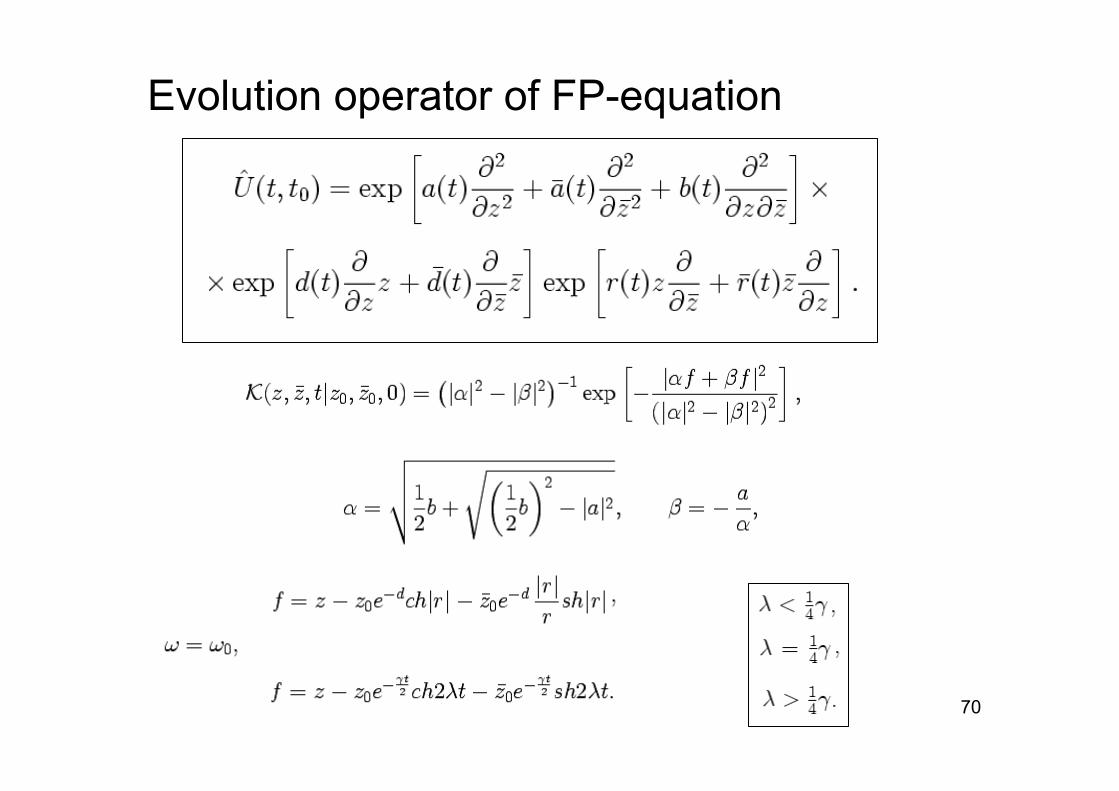
Evolution operator of FP-equation

71

The case of zero detuning

72

Nonzero detuning

73

Summary and some problemsWe have presented a mathematical formalism for describing the dynamics and relaxation of quantum systems. Group theoretical method and the CS technique are naturally used in quantum optics, quantum information theory, condensed matter and so on. Search for quantum corrections to the semi-classical dynamics CS in this approach in the general case has not been solved to date.One of the main problems here is the inclusion of non-Markovian effects into consideration.Possible generalizations of the concept of dynamical symmetries (super-algebras, associative algebras, …) to more complicated and realistic systems also a worthy of special consideration.

74

AcknowledgementsI’m sincerely grateful to my former students and colleagues (Ilya Sinayskiy, Vitaly Semin, Elena Rogacheva, Viktor Mikhailov, Slava Ruchkov, Vadim Asnin, Dmitriy Umov,…). The collaboration with them was very helpful for me!

I am also very grateful to Professor Francesco Petruccione for his kind invitation and for the opportunity to spend the amazing month in Durban!

75

Thank You!

z