nmof fixed income review – final report - … · nmof fixed income review – final report . ......
TRANSCRIPT

NMoF Fixed Income Review – Final Report Stephen Schaefer & Jörg Behrens 29 March 2011
Acknowledgement:
The authors gratefully acknowledge helpful suggestions and comments from Christof Schmidhuber

Review of Fixed Income Investments Page 2

Review of Fixed Income Investments Page 3
Contents 1. Executive Summary ..................................................................................... 5 1.1. Objectives of the Report ............................................................................. 5 1.2. Systematic Risk Factors for Fixed Income ................................................... 5 1.3. Review of Management Model ................................................................... 7 2. The Composition of the GPF-Global Portfolio ........................................... 10 2.1. The Role of Bonds in the Fund’s Portfolio ................................................. 10 2.2. The Global Fixed Income Market and the Coverage of the Barclays Global
Aggregate Index. ....................................................................................... 16 3. The Analysis of Factors and their Premia .................................................. 19 3.1. Overview and Introduction ....................................................................... 19 3.2. Relevant Systematic Risk Factors in the Fixed Income Market and their
Properties .................................................................................................. 19 3.3. Factors used in the Empirical Analysis ...................................................... 22 3.4. Properties of these Factors ....................................................................... 24 4. Risk Factor Exposure in the Current Benchmark ...................................... 41 4.1. Risk Factor Exposures and the Stability of Risk Exposures over Time ...... 41 5. Core & Satellite Model .............................................................................. 47 5.1. Overall Set-Up ........................................................................................... 47 5.2. The Core .................................................................................................... 49 5.3. The Satellites ............................................................................................. 50 5.4. Choice of Satellites .................................................................................... 51 6. Management Model .................................................................................. 54 6.1. Current Setup ............................................................................................ 54 6.2. Proposed Scheme: Formulation of the Mandate ...................................... 55 6.3. Proposed Scheme: Challenges .................................................................. 58 6.4. Proposed Scheme: Benefits ...................................................................... 59 7. Risk Budgeting and Asset Rebalancing ...................................................... 61 7.1. Asset Rebalancing between the Fixed Income Core and Risk Assets ....... 61 7.2. Risk Allocation at the Portfolio Level ........................................................ 62 7.3. Definition of Risk Budgets and Asset Rebalancing within Satellites ......... 63 7.4. Risk Budgeting Approach and Allocation - Reviewing the Choices ........... 65 8. Benchmark Construction ........................................................................... 66 8.1. Benchmarks are Incentive Schemes .......................................................... 66 8.2. Benchmark Construction - Available Options ........................................... 68 8.3. Market-implied Benchmarks ..................................................................... 68 8.4. Core Portfolio Benchmark ......................................................................... 69 8.5. Satellite Setup Processes and Benchmark Definition ............................... 71 9. Conclusion and Outlook ............................................................................ 76

Review of Fixed Income Investments Page 4

Review of Fixed Income Investments Page 5
1. Executive Summary
1.1. Objectives of the Report
This report deals with two important questions regarding the management of the fixed income component of the Government Pension Fund (the Fund). The first concerns the composition of the fixed income benchmark portfolio and the second addresses the management model.
In addition to this Executive Summary, the report contains seven main sections and a conclusion. Sections 2, 3 and 4 are devoted to the composition and risk characteristics of the portfolio and 5, 6 and 7 to the management model. Section 8 deals with the composition of the fixed income benchmark. In addressing the first question, the starting point is a discussion of the role that fixed income plays in the overall portfolio. Is it to reduce overall risk, to generate a risk premium or to hedge the Fund’s liabilities?
To answer these questions the report first identifies the risk factors to which fixed income assets are exposed. It then goes on to estimate their risk and return characteristics and the exposure of different asset classes to these factors.
Several categories of fixed income assets, e.g., asset-backed securities and corporate debt, have exposure to so-called long-tailed risk factors, i.e., those that exhibit little variability for much of the time but occasionally give rise to severe losses. Liquidity risk and volatility risk have these characteristics. An important problem that this raises for the management of the Fund is that relying on the standard deviation of the tracking error as a method of controlling risk may be inadequate unless the exposure to different types of risk is also monitored. Sections 5, 6 and 7 address this question and suggest a solution that, so far as possible, isolates the Fund’s exposure to long-tailed risks in satellite funds and allows the core fund to invest only in assets with risk factors that are not expected to have this feature.
1.2. Systematic Risk Factors for Fixed Income
The bond portfolio contains a very large number of positions. At the same time many different types of bonds are influenced by the same types of risk; for

Review of Fixed Income Investments Page 6
example, almost all bonds are strongly affected by interest rate movements. It is therefore useful to discuss the risk profile of the bond portfolio mainly in terms of “factors”, i.e., systematic influences on returns, and “factor exposures”, the sensitivity of returns to these factors, rather than asset categories or, still less, individual positions.
A primary objective of the Fund is, subject to constraints on risk, to maximise its long-run return, and the exposure of fixed income assets to factors that have non-zero risk premia provides an opportunity for the Fund to deliberately take exposure to these factors in order to “harvest” the risk premia. In principle this is a sound strategy for the Fund to pursue but there are a number of issues to be addressed.
A second role for the bond component of the Fund is simply to lower the overall volatility of the portfolio. Most government bonds preserve value better than non-government bonds but this effect is significant only in major crises and the value of this type of liquidity may be of lower value to an investor, such as the GPF, that has no leverage, a long horizon and little immediate need for cash.
A third potentially important role for bonds in the portfolio is as a source of liquidity both for rebalancing and the Fund’s long-term future cash outflows. The timing and risk characteristics of these outflows have implications for the choice of benchmark and this point is taken up in Section 4 of Chapter 8.
Section 3 of the report identifies the key risk factors that drive returns in fixed income markets and estimates their risk and return characteristics. The most important factor in terms of overall variability is the government yield curve. For the BGAI this accounts for almost 90% of the monthly variation. However yield curve factors do not provide strong evidence of risk premia: the average premium of long-term bonds over Treasury bills in both the US and the UK is around one percent per year, a number that cannot be statistically distinguished from zero even with 100 years of data.
The factors analysed in this section include the Fama-French factors, credit spreads, a liquidity factor and two volatility factors. One of these, the returns on variance swaps, has a large historical risk premium, relatively low volatility on average and occasional very large drawdowns. Given its large risk bearing capacity, the Fund may have a competitive advantage in bearing this type of risk.
Section 4 estimates the sensitivity of the Main asset categories represented in the BGAI to the factors identified in Section 3. To protect the Fund from inadvertent
Review of Fixed Income Investments Page 7
exposure to risk factors with long left tails, it is important that the factor exposure of the various assets be both measurable and measured.
Overall the results in this section are encouraging and lead to a number of useful conclusions. First, assets may have risk exposures that would not be expected given the nature of their cash flows. One example here is the equity exposure of US agency debt. Second, many apparently different asset classes have exposure to common factors and, in particular to the returns on variance swaps, liquidity and, again, the stock market. Third, the exposure of the Fund’s active returns changed markedly over time, moving from tracking the benchmark very closely indeed to having quite significant interest rate and liquidity exposures in the period leading up to the crisis. The results suggest that these and other risk exposures can be usefully measured.
1.3. Review of Management Model
The GPF benefits from the fact that it has an indefinite investment horizon and, as long as oil revenues exceed fund outflows, it has almost no liquidity constraints. This makes it an ideal risk taker with tremendous risk bearing capacity for many types of financial investment risks.
In the 2008 crisis, while the absolute return on the Fund’s fixed income portfolio was close to zero, gains in high-quality, highly liquid assets such as AAA government bonds were offset by an unexpectedly large underperformance relative to the benchmark, a fact which Ang, Goetzmann and Schaefer (2010), in a previous report, found could be attributed to exposure to heavily left-tailed risk factors that had not been apparent.
In chapter 5ff. we will propose an improved management mandate with the particular objective of institutionalising a structure that allows the Fund to deal will the challenges that may well resurface in the next market crisis. This structure will ensure that drawdowns in stress situations remain within expected ranges while the Fund can still exploit the full potential of its risk bearing capacity.
The following steps seem crucial in progressing towards this objective:
• Non-standard risks need to be separated from the core portfolio so that they are better understood, and in order to create incentives that are consistent with the dual objectives of the fixed income portfolio.

Review of Fixed Income Investments Page 8
• Clear rules must be put in place to decide whether particular non-standard risks represent a desirable investment, should be hedged or entirely avoided. These rules must account for low variance / long-left-tail characteristics. The investment mandate needs to distinguish between index tracking and risk taking mandates in order to reflect the different nature of the risks taken, and the incentives of managers must be aligned with the objectives of their mandates, i.e. either to track an index where the objective is a minimal tracking error or to take a specific risk according to a clearly defined set of rules.
In chapter 5, the authors propose a core satellite approach to split the management mandate into two parts, one addressing a "core" investment portfolio comprising high quality fixed income investments and the other an additional "satellite" mandate (implemented by NBIM through a small number of separate satellites) to take some specific, desired fixed income risks. This approach allows separation of the dual objectives of the fixed income portfolio and setting the correct incentives for them both: The “insurance” function of holding highly liquid bonds is placed into the core portfolio, and the “income” function is provided by one or more dedicated satellites actively seeking exposure to risk factors such as credit, liquidity and volatility - in order to monetise the risk bearing capacity of the GPF.
The benefits of the core satellite approach are not only to be seen in increased transparency, but also through improvements in the effectiveness of risk control, and in the ability to include exposure to risk factors that are consistent with the Fund’s risk appetite. This means that the Ministry will, first, be able to define the overall risk budget and will thus limit the total amount of risk that can be taken. Secondly, the explicit handling of all non-core risk factors in a separate portfolio will enforce an effective culture of dedicated investment and risk management that has so far been applied by NBIM mainly in dedicated “alpha” mandates. The core satellite approach thus results in a transparent and positive “competition among investment risk factors” where the most “profitable” risk factors relative to the allocated risk budget will prevail, possibly resulting in a better performance with a clearly controlled and limited overall level of risk.
The satellite risks already present in the current portfolio, in particular credit, liquidity and volatility, could at a later time be supplemented with a number of other satellite investments such as insurance risks, which may have favorable diversification effects. Overall the result is a more favourable risk reward profile for the Fund while minimising the opportunity for taking opaque investments.

Review of Fixed Income Investments Page 9
In the new management model the incentives of all stakeholders will be better aligned as investments into non-core risk factors will be based on a conscious risk/reward analysis within a dedicated and controlled satellite portfolio.

Review of Fixed Income Investments Page 10
2. The Composition of the GPF-Global Portfolio
2.1. The Role of Bonds in the Fund’s Portfolio
Currently 40% of the GPF benchmark portfolio is allocated to bonds. Going forward, the fixed income allocation will be reduced gradually towards 35% to accommodate a real estate allocation of up to 5 per cent. What role do bonds play in the overall portfolio? Is 35% the right proportion? And, within the bond component of the benchmark, is the allocation to government bonds, agency bonds, corporate bonds etc. optimal?
In simple terms, bonds might be considered the “riskless asset” in the standard portfolio selection model: the investor chooses the proportion of the portfolio to be allocated to risky assets (say, stocks) with the remainder invested in the riskless asset (bonds). For example, if 40% of the portfolio is invested in the riskless asset, then, since the riskless asset is assumed to have a rate of return volatility of zero, the portfolio volatility is 60% (100% - 40%) of the volatility of an all-stock portfolio. In the same way, since the riskless asset has, by definition, a zero risk premium, the risk premium on the portfolio in this example is also 60% of the risk premium of an all-stock portfolio.
While clearly oversimplified, this simple framework does say something useful about role of bonds in the GPF portfolio. Overall, bonds do have both a lower risk premium and a lower volatility than equities and so, by investing part of the portfolio in bonds the risk of the overall portfolio is lowered along with the risk premium. From this perspective the decision about the proportion of the GPF to be invested in bonds reflects the risk appetite, or tolerance of the Fund for equity risk.
This simple story ignores three important aspects of bond investment. The first is the term or maturity of the bonds in the portfolio. The second is the pattern of risk exposures that accompanies investment in different types of bonds and the third is liquidity. We discuss each of these in turn.
Maturity In the simple bond-stock portfolio example the investor’s horizon is just one period. What this means is that the investor cares only about the market value of the portfolio at the end of the period (e.g., one year) and has no interest in how this portfolio will provide for consumption in the longer run.

Review of Fixed Income Investments Page 11
This short-term perspective is far removed from the objective of the GPF which is to support the long-run pension needs of the Norwegian people. The time horizon of the Fund is very long indeed and the maturity composition of the Fund is therefore potentially important. Long term bonds, particularly long term inflation linked bonds, may help to hedge long-term consumption needs and, in this case, the risk borne by the Fund cannot be measured simply in terms of short-term fluctuations in value (since the value of the Fund’s future cash outflows are correlated with the value of the bond portfolio). Even though they have higher volatility, long-term bonds may therefore serve an important purpose in the portfolio (hedging) whether or not they provide a risk premium.
Risk Exposure The bond portfolio contains a very large number of positions. At the same time many different types of bond are influenced by the same types of risk; for example, almost all bonds are strongly affected by interest rate movements. It is therefore useful to discuss the risk profile of the bond portfolio mainly in terms of “factors”, i.e., systematic influences on returns, and “factor exposures”, the sensitivity of returns to these factors, rather than asset types or individual positions.
The fixed income portfolio currently held by the Fund has a relatively low exposure to credit risk and, largely for this reason, the main drivers of return are the government yield curves in the countries in which it is invested. Between 80% and 90% of the variance of the returns on the BGA index is explained by just two return series: long term US Treasuries and long-term Euro-denominated government bonds.1
The evidence in support of significant long-term risk premia from exposure to government yield curves is not strong. (The evidence is discussed in detail in Section 3.4). Because yield curve risk is the single most important source of risk for the bonds currently in the Fund’s fixed income investment universe, if these risks are not rewarded by a risk premium it raises the question of whether it makes sense for the Fund to have these exposures.
Since over 60% of the index consists of debt that is either issued or guaranteed by government, with the remainder having relatively little default risk, this is not a surprise.
1 Unless stated otherwise, all the analysis in this report is carried out on returns that are hedged against currency fluctuations.

Review of Fixed Income Investments Page 12
One possible rationale has already been discussed, namely that long term bonds may hedge the Fund’s future cash outflows or liabilities. Or, to put the same point another way, changes in the value of the Fund’s future cash outflows may be correlated with the yield curve. However, a more extensive analysis of this important issue lies outside the scope of this report.
While the yield curve represents the largest single source of risk in the Fund’s fixed income portfolio, other risk factors are also important. These include credit risk, liquidity risk, volatility risk and others. The properties of these factors and the corresponding factor exposures of the BGAI are discussed in Sections 3 and 4 below.
The exposure of fixed income assets to these various factors, combined with non-zero risk premia (in some cases) provides an opportunity for the Fund to deliberately take on factor exposure in order to “harvest” the risk premia. In principle this is a sound strategy for the Fund to pursue but it also raises a number of issues.
The first is the appetite that the Fund has for different types of risk; in principle resolving this issue is no different from the Fund deciding on the allocation between bonds and equity. The second is the difficulty that always exists in estimating the size of the factor risk premia. A third difficulty, linked to the second, concerns the distribution of returns on a factor. During the crisis some factors, e.g., volatility, which appeared to offer high risk premia with relatively low risk had drawdowns over a few months that were large enough to offset several years of gain. Finally, for some factors it is difficult to estimate the exposure of an instrument or portfolio to that factor. As a result, a portfolio may turn out to have unplanned exposure to a factor or, conversely, to lack exposure in cases where positive or negative exposure had been planned. All these issues are discussed in more detail in Sections 3 and 4.
Any portfolio remotely similar to the Fund’s current fixed income portfolio will have exposures to a variety of risk factors and it is important that these exposures are monitored as precisely as possible. During the crisis one of the reasons – probably the main reason – for the Fund’s poor performance relative to its benchmark was the fact that it had unplanned exposure to factors such as liquidity and volatility and that these factors had large drawdowns in the crisis.
The Multi-Factor Setting and Diversification
Review of Fixed Income Investments Page 13
In a world where asset returns are driven by multiple factors and investors are interested in hedging future consumption, the market portfolio is not necessarily the optimal portfolio for all investors.
This statement holds quite generally, e.g., for equities as well as bonds, but there is an important qualitative difference between equities and the majority of bonds. This is the fact that, for a typical equity, a large fraction of the risk is idiosyncratic while for most bonds it is not. The presence of substantial idiosyncratic risk in equities means that there is always a strong imperative to diversify while, for most bonds, there is not. Thus, in general, there is more scope in a bond portfolio than a stock portfolio to acquire risk exposures that deviate from the benchmark without, at the same time, acquiring significant tracking error.
However, diversification does have an important role to play in parts of the fixed income portfolio. First, in credit markets idiosyncratic risk can be significant, especially for bonds outside the highest credit categories. Second, for some developed countries sovereign risk has emerged as a potentially important issue in the last few years and this may also provide a motivation for diversification.
Credit Exposure An important insight from the large amount of research that has been carried out on credit risk over the past few years is that the risk of default and the pricing of credit risk are related but distinct issues2
Accordingly, one of the objectives of this study is to identify the factors that influence the return on the Fund’s FI portfolio and estimate their risk and return characteristics.
. The risk of default appears to be relatively well explained by fundamentals, in particular by corporate leverage, measured in terms of the market value of a firm’s equity, and the volatility of its asset value. According to contingent claims theory, these same variables should explain credit spreads, but a succession of research studies has found that yield spreads on credit risky bonds are (a) typically larger than those predicted by the Merton model and its variants and (b) also influenced by other factors including liquidity proxies and the Fama-French factors.
As already discussed, one possible role for credit risky debt is to provide the Fund with exposure to these factors. Overall, if there are risk premia attached to these
2 Huang & Huang (2003), Schaefer & Strebulaev (2009), Collin-Defresne, Goldstein & Martin (200

Review of Fixed Income Investments Page 14
factors then this provides one motivation for taking credit exposure. These questions are addressed later in the report.
Liquidity An important characteristic of government bonds is that in periods of market stress they maintain liquidity, and value, better than other assets. This was seen strikingly in the recent crisis where the spread between, for example, high grade corporate debt and government debt rose to levels that appear (then and now) to be unrelated either to the objective risks of default or to a risk premium that is consistent with empirical estimates of the “beta risk” of corporate debt.3
Government debt is often described as a “store of value” in a crisis, a characteristic that is valuable to many market participants and provides a motivation for holding government debt that is quite separate from any risk premium it might offer. The value of government debt liquidity differs across market participants. For investors with fixed liabilities, particularly those liabilities with uncertain cash flow timing, e.g., banks, it can be very valuable indeed. For the Fund, which has few fixed obligations and a positive net cash flow for the medium term, the value of liquidity may be generally much smaller.
4
In a crisis, however, the liquidity of the bond portfolio plays an important role since the value of the equity portfolio is likely to fall by much more than the fixed income portfolio. If, under these conditions, the Fund wishes to maintain its target allocation to equities and bonds, it will need to sell some bonds in order to be able to buy equities. It follows that if the risk preferences of the Fund dictate that it allocates less than 100% to equities, the bonds that it does hold must be sufficiently liquid to be sold at non fire-sale prices under conditions when equity prices may have fallen sharply.
It is also useful to put the “value preservation” services of corporate debt into context. Figure 1 shows the results of the following calculation: monthly returns on long-term US government debt are regressed on monthly returns on long-term US corporate BBB debt to calculate the monthly “predicted” return on government debt conditional on the corporate debt return. Next, the “surprise” in the return on government debt is calculated as the difference between the actual return and the predicted return. Figure 1 then plots the monthly “surprise” against the corporate return.
3 Huang & Huang (2003) & Schaefer & Strebulaev (2009) 4 Krishnamurthy (2010) discusses the “store of value” characteristics of government debt.

Review of Fixed Income Investments Page 15
The figure uses data from the past 37 years (Jan-1973 to Jun-2010) and the area of most interest is the left hand part of the figure, i.e., when corporate returns are negative. Here, we see that, for modest falls in the bond market of 5% or less, the surprises in government bond returns are as often negative as positive. (For BBB returns of between 0% and -5% the average surprise in the government return is a negative 0.5%). It is only for very large monthly falls in the corporate market that government bonds perform much better on a consistent basis. Altogether, out of the 449 months of data included in the Figure, there are just five months where the behaviour of the return on government bonds clearly exhibits the “store of value effect” described above. These months are marked in the figure: there are two months from 1974, two from 1979-80 and one from the recent crisis. However, for the two months in the 1979-80crisis, when the BBB index fell by 9.0% (Oct-79) and 8.0% (Feb-80) government bonds did little better than normal (0.96% and 0.66% respectively).
There are therefore only three months over the past 37 years when (i) US corporate debt has fallen by more than 5% in one month and (ii) government bonds have performed significantly better than normal. Two of these months were in the 1974 crisis and the one remaining month was in the recent crisis.
Summary The bond component of the GPF portfolio lowers the overall volatility of the portfolio. For the relatively high quality bonds that the GPF holds this applies to both government and non-government bonds. Government bonds preserve value better than non-government bonds, but this effect is significant only in major crises and the value of this type of liquidity is of less value to an investor, such as the GPF, that has no leverage, a long horizon and little immediate need for cash. Within the government component of the portfolio, more attention currently needs to be paid to sovereign default risk than was probably necessary in the past and this may well provide a motivation for diversification across countries and currencies. Long-run nominal bonds, while a hedge against deflation, are subject to inflation risk. Since some major holders of government debt have liabilities that are denominated in real terms, e.g., pension funds with benefits linked to final salary, the demand for inflation protection may result in inflation linked bonds providing lower returns than nominal bonds.5
5 See Wright (2008)
If the Fund’s main purpose in holding government bonds is as a source of liquidity rather than hedging, this

Review of Fixed Income Investments Page 16
suggests that inflation linked bonds may not play an important role in the portfolio.
2.2. The Global Fixed Income Market and the Coverage of the Barclays Global Aggregate Index.
The Barclays Global Aggregate Index (BGAI) aims to provide a broad-based measure of the global investment grade fixed-rate debt markets. The Global Aggregate Index family includes a wide range of standard and customised sub-indices categorised by liquidity, sector, quality, and maturity. The Global Aggregate Index was created in 1999, with index history backfilled to January 1, 1990.
The Barclays Global Aggregate Index Criteria for Inclusion
The two main criteria for a bond’s inclusion in the BGAI are a liquidity requirement, expressed in terms of the size of the issue, and a quality threshold, expressed in terms of the rating. In addition, constituents must have a remaining maturity of at least one year and coupons must be fixed rate. Bonds with any form of equity dependence – e.g., convertibles – are excluded, as are floating rate notes, warrants and structured products.
Table 1 shows the composition of the BGAI in terms of the main geographic regions. The index currently contains over thirteen thousand issues of which just under ten thousand are either US or Euro area issues. In terms of the amount outstanding (columns 2 and 4) these two regions account for 38% and 34% respectively of the total of over $36 trillion. The weighted average maturity of the index is currently just over 7.5 years. The modified duration of the BGAI as of February 2011 is 5.68 years.
If the objective is to construct a “market portfolio” of the world’s bond markets then the BGAI fails in a number of respects. For example, a market portfolio would include some of the instruments currently excluded, such as bonds with a maturity of under one year and floating rate bonds. But does it make sense for the Fund to aim to hold the world market portfolio for bonds?
As described earlier in this report, the need to diversify, so critical in equity markets, is much less strong in bond markets. Within a high quality bond portfolio – and the average quality of the BGAI is around AA (Figure 2) – the return on a

Review of Fixed Income Investments Page 17
portfolio chosen from a large set of bonds can usually be quite closely replicated by a portfolio chosen from a much smaller set. For example, in liquid government bond markets (e.g., the US) two factors typically account for substantially all of the variation in the prices of individual bonds and this implies that a portfolio containing just two bonds (and cash) is able to replicate closely the return on a portfolio containing a large number of issues.
Neither equity nor bond investors usually choose to hold a portfolio with a very small number of securities, but the reason in the two cases is different. An equity investor would diversify extensively because not to do so would mean adding substantially to the risk of the portfolio without a compensating increase in the expected return. For a bond investor – again for high quality bonds – the risk reduction benefits of diversification are relatively modest.
Most high quality bond portfolios contain many positions for reasons related to liquidity rather than diversification. If a large position is taken in a particular bond issue it may well be costly, in terms of transaction costs, both to acquire the position initially and to sell it prior to maturity.
“Optimal” Bond Portfolios By constructing a portfolio that avoids very small issues (the size requirement) and holding bonds in proportion to the amount outstanding the BGAI avoids these illiquidity costs, but this does not by itself imply any form of portfolio optimality.
As described earlier, one of the potential roles for the Fund’s bond portfolio is to hedge its future cash outflows. This means that the Fund’s portfolio must be chosen to reflect the particular risk characteristics of these cash outflows. Other investors will have different needs and this will result in portfolios with different composition and, different duration. When assets, such as bonds, provide investors with the opportunity to hedge, different investors will choose different portfolios. One size, in this situation, does not fit all.
If Fund were to use the fixed income component of the portfolio to hedge, it would mean targeting particular factor sensitivities, e.g., duration. However, duration changes over time with the level of interest rates and so, even if the BGAI happened to have the right level of duration for the Fund at one point in time, there is no guarantee that this would be the case when interest rates change or time simply moves forward.
Summary

Review of Fixed Income Investments Page 18
The BGAI is a broadly based, well diversified bond portfolio with a low exposure to credit risk. Its rules for inclusion and exclusion mean that it is feasibly investable and, by the standards of bond markets, relatively liquid. The BGAI’s relatively low volatility and attention to liquidity are valuable to the Fund. However, there is no reason to think that the BGAI’s particular pattern of exposure to the main risk factors driving its return – yield curves, and credit spreads – is necessarily optimal, or even suitable for the Fund.

Review of Fixed Income Investments Page 19
3. The Analysis of Factors and their Premia
3.1. Overview and Introduction
This section of the report addresses some key questions concerning the composition and management of the Fund’s fixed income portfolio and continues the line of analysis developed in the earlier study by Ang, Goeztmann and one of the present authors (AGS). AGS proposed that the Fund’s exposure to systematic “non-standard” factors should play an important role in both performance measurement and the construction of the benchmark. A key objective of this report is to consider how this approach might be implemented for the Fund’s fixed income investments.
The purpose of the Fund is to support government savings to finance pension provision for current and future generations of Norwegians. It seeks to achieve the “best possible trade-off between return and risk”.6
3.2. Relevant Systematic Risk Factors in the Fixed Income Market and their Properties
One consequence of multi-factor framework – as distinct from the standard CAPM setting – is that the Fund needs to take into account that it may have a different appetite for different types of risk. For example, it may have a high tolerance for interest rate risk but not for volatility risk since the economic conditions under which losses would occur may be different. Thus the trade-off between risk and return that is best for the Fund may be different for the different types of risk. These are questions for the Fund’s owners but, whatever the answers to these questions, it cannot be assumed that the relevant measure of risk for the portfolio is a simple aggregate statistic such as the volatility of the return on the Fund.
In a well diversified portfolio the great majority of the risk is systematic rather than idiosyncratic. This is true in equity markets even though, at the individual security level, a large fraction of the risk is idiosyncratic. It is even more true in fixed income markets where, at least for investment grade bonds, the great majority of the risk at the individual security level is systematic.
For a given portfolio, one objective of identifying the relevant risk factors is, therefore, simply to describe and measure the risks of the portfolio. These will usually be expressed as “betas”, or price elasticities, measuring the sensitivity of
6 Project brief.

Review of Fixed Income Investments Page 20
an asset’s value to movements in a given factor. As described earlier, the economic nature of the risks represented by each factor may be quite diverse and an investor may have a high tolerance for one type of risk and a low tolerance for another.
Each risk factor will have a risk premium (positive, negative or even zero) and the overall risk premium on the portfolio is simply the sum of the individual premia weighted by the portfolio betas. The problem of choosing a well-diversified portfolio may therefore be thought of in terms of choosing the betas, i.e., the level of exposure, to each of the factors; these determine both the risk premium on the portfolio and its risk profile.
To implement this approach it is therefore necessary to:
• Identify the relevant factors, their volatilities and correlations;
• Estimate the risk premium on each factor; and
• Estimate the sensitivity of the portfolio to each factor.
This section first describes the risk factors and then gives estimates of their risk premia and other properties. Section 4 below gives estimates of the sensitivity of the BGAI and its major components to the factors.
One of the aims of this study is to provide advice that would assist the Fund in deciding whether it should, as a matter of policy, include exposure to particular factors in the benchmark. To this end we discuss the factors that are relevant to pricing fixed income assets and describe the distribution of their returns.
As described below, the factor approach is routinely applied in one form or another to analyse the term structure of government yields. It has also been used to analyse fixed income returns in the context of performance measurement (Brown and Marshall (2001), Chen, Ferson and Peters (2010)), asset pricing (Baele, Baekaert and Inghelbrecht (2007), Fama and French (1993)) and capital structure arbitrage (Schaefer and Strebulaev (2006)).
Existing Evidence on the Factor Structure of Fixed Income Returns For government bonds there is extensive research, using data from many countries on the factors driving the yield curve (and, therefore, returns). Often these factors are chosen to be the “level” and “slope” of the yield curve.7
7 Litterman & Scheinkman & Weiss (1991)
The specific maturity characteristics of these factors will depend on the range of maturities represented

Review of Fixed Income Investments Page 21
in the data but, broadly speaking, the “level” factor will be a rate of intermediate maturity (relative to the data under investigation) and the slope factor will be the difference between a long term and a short term rate.
In liquid government bond markets, these two factors together typically explain in excess of 95% of the variation in both changes in the yield curve and, because the level of idiosyncratic risk is small, actual returns on bonds. The overall risk premium from yield curve exposure is discussed below in Section 3.3. There is evidence that the slope factor is itself a predictor of future returns, i.e., of time varying risk premia.8
In liquid government bond markets, e.g., the US and major European countries, the part of the return not explained by the level and slope is small and has negligible exposure to other factors.
9
The results of the empirical analysis of factor exposures in Section 4 are more easily interpreted when the factors used are investable. For this reason we use returns on long-term and short-term bond indices as factors rather than the level and slope of the yield curve.
Corporate Credit Markets The existing literature on credit risky corporate bonds includes both theory and empirical work. For the issues addressed in this report the most useful theoretical framework is the so-called structural approach which treats both the debt and equity of a firm as contingent claims on its assets. Equity has the character of a call on the assets; holding a corporate bond is similar to holding riskless debt and having written a put option on the firm’s assets.
According to this framework the risk factors that should appear in returns on credit risky debt are (a) those that drive the government yield curve (level and slope) and (b) the value of the firm’s assets. The latter is highly correlated with equity. What the data show is that these factors are indeed significant drivers of return but other factors that are inconsistent with the theory are also significant. These include the Fama-French factors, volatility and the S&P. The results in
8 Fama & Bliss (1987) 9 There are well-know liquidity related frictions in these markets (e.g., those connected with repo-specialness) and this may influence the Fund’s decisions on of precisely which securities to hold. However, these effects are small and, in our view, not best handled via a factor approach.

Review of Fixed Income Investments Page 22
Section 4 show that the corporate debt segments of the BGAI are significantly related to these same factors.10
Other Debt Securities
The BGAI also contains other categories of debt, in particular government related (e.g., agency) bonds and asset backed securities. Prior to the crisis the debt of US government agencies such as Freddie Mac and Fannie Mae, though not formally guaranteed by the US Treasury, was generally regarded as virtually default free, and the difference between the pricing of agency and Treasury debt was typically ascribed to liquidity. However, the events of the recent crisis have called into question the creditworthiness of agency debt.
Finally, the asset backed securities market includes issues with a wide variety of collateral types (including mortgages, credit cards, auto loans etc.). Factors related to liquidity, volatility and asset value may be expected to be related to returns on these asset classes.
Correlation between Factors Our empirical analysis in Section 4 will show that some securities have a significant exposure to risk factors that appear to be unrelated to the asset in question. A good example is provided by the returns on US Government agency securities which are strongly related to the S&P despite having no obvious connection with the equity market.
While this might appear puzzling it is important to remember that many of the factors we consider are correlated and so it may be misleading to over-interpret the economic character of a particular factor. Moreover, the return on a security also reflects fluctuations in the risk premia and these are likely to be correlated across asset categories, even if the cash flows are not.
3.3. Factors used in the Empirical Analysis
The factors used in the empirical analysis fall into three groups:
• Returns on long and short government bonds;
• Stock market returns (in particular, the S&P 500); and
• Volatility and other non-standard factors (see below).
In the empirical analysis carried out so far the following factors have been used:
10 Collin-Dufresne, Goldstein & Martin (2001) and Schaefer & Sterbulaev (2008).

Review of Fixed Income Investments Page 23
Government Bond Returns:
• Return indices on (i) medium/long term bonds and (ii) 1-5 year bonds in the US, UK, the Euro-zone, Asia and Japan. Source: BarCap.
Volatility and other non-standard factors
• Fama-French factors: The standard SMB, HML and MOM factors. (Source: Ken French’s website).
• Liquidity: The spread between REFCO and Treasury 10-year STRIP yields. (Source: Bloomberg).
• Volatility: The VIX index. (Source: CBOE).
• Volatility: Returns to equity variance swaps. (Source: CBOE (VIX) and own calculations. See below).
• Credit Spread: The difference between the yield on BBB and AAA corporate debt. (Source: Moody’s – from US Treasury website).
Stock market indices
• Returns on the S&P 500, FTSE All-share, EuroStoxx, Nikkei 225 and S&P Asia indices. (Source: Morningstar/DataStream).
The Volatility Factors The empirical analysis uses two related, but distinct volatility factors. The first is the well known VIX index that was introduced in 1993 as the implied volatility on short-term at-the-money options on the S&P 100. In 2003 the index was redefined as a (different) function of option prices (on the S&P 500) that gives the fair value of the fixed payment on a one-month “variance swap” that pays fixed and receives the actual realised variance on the S&P 500.11
The second volatility factor is the return on this swap, i.e., the difference (or log difference) between the realised variance and the VIX. Subject to variance swaps being actually priced at the VIX, this second factor is actually tradable. The VIX factor by itself does not represent the return on any particular strategy but VIX futures are traded and the risk characteristics of returns on the future are likely to be similar to the factor used here which is the first difference of the VIX index.
Liquidity Factors
11 Despite the difference in definition between the old and new versions of the VIX, their values are quite similar.

Review of Fixed Income Investments Page 24
Although there has recently been an upsurge in research on liquidity in financial markets, financial economics is still some distance from developing a comprehensive model of liquidity risk with quantitative predictions. A good description of the state of the art is given in Amihud, Mendelson and Pederson (2005). Dick-Nielsen, Feldhutter and Lando (2010) and De Jong and Driessen (2006) analyse liquidity effects in corporate credit markets.
The liquidity factor used in this report is the difference between the yields on 10-year REFCORP STRIPS and 10-year Treasury STRIPS. REFCORP bonds were issued in the wake of the S&L crisis of the late 1980s and early 1990s and are, in effect, guaranteed by the US Treasury. The difference in yield therefore primarily reflects liquidity.
AGS used the yield spread between the on- and off-the-run 10-year Treasury as a liquidity proxy. This behaves in a broadly similar manner to the REFCORP – Treasury spread (see Figure 3) and there is no theoretical reason to use one or the other.12
In the regressions – as in AGS – the liquidity measure is used in the form of the change in yield spread rather than as a rate of return. In this form the liquidity proxy is not investable. It would be possible to compute the return from a long position in the REFCORP bond and a short position in the Treasury but, computing the achievable rate of return would involve knowing the borrowing costs for the Treasury security and these data are not currently available.
Credit Spreads. We use the difference between the yield on BBB and AAA US corporate debt as a credit factor. AAA corporate debt was used as the benchmark rather than Treasury debt to abstract from liquidity effects in Treasuries.
3.4. Properties of these Factors
In this section we describe the properties of these factors in terms of the distribution of their historical returns and the correlation between them. Because the properties of stock market returns are relatively well understood, attention will be focussed on the factors driving government bond returns, volatility, liquidity and credit.
12 The yield spread between the on- and off-the-run 10-year Treasury is a proprietary series produced by the Treasury and was not available for the whole period covered by this study. Another possibility would have been the LIBOR-OIS Spread but this has only a short history. See Sengupta and Yun (2008).

Review of Fixed Income Investments Page 25
The complete list of the 20 factors used in our analysis is given in Table 2. The first eight are the returns on Government bonds, the next seven include the three Fama-French factors, two volatility measures, the liquidity proxy and the credit spread and the remaining five are returns on national and regional stock indices.
The objective of this section is to assess the risk and return characteristics of the factors that are used in the next section to estimate the risk exposures of the BGA index. We begin with an analysis of risk premia in government bond markets. In the remainder of this section, since the properties of stock market returns are well understood, we focus on the Fama-French factors, liquidity, credit spreads and, particularly, on volatility.
Government Yield Curve Risk Premia Because a large fraction of the variability of the BGAI is explained by government rates, an important question for the Fund is whether it should expect a positive risk premium for bearing these risks specifically.
The available data show that the risk premium on government bonds has been small. Using a one hundred year history, Dimson, Marsh and Staunton (2000) found the premium on long term US Treasury bonds to be 0.7% (Table 3) and, importantly, that this estimate was slightly smaller than one standard error from zero. For the UK the mean premium was slightly higher but also within one standard error from zero. In other words, even 100 years of data would be insufficient to convince a sceptic that government bonds in the US or the UK provide a premium over Treasury bills.13
With the reduction in inflationary expectations over the past 10-20 years and the resulting fall in long-term nominal rates, long bonds have recently outperformed short bonds. Table 4 provides estimates of the risk premia on US Treasury bonds of different maturities and shows that between 1952 and 2010 10-year bonds earned an annual premium over Treasury bills of 1.79% (panel (e)). The t-statistic on this figure is 2.35. However, this positive premium is largely due to the behaviour of interest rates over just the past ten years; excluding the period from January 2000 onwards, the premium falls to 1.34% and is statistically insignificant (panel (d)).
13 The predictions of the various classical term structure hypotheses accommodate virtually every possible pattern of risk premia. For example, (one version of) the pure expectations hypothesis predicts that risk premia are zero and the liquidity preference hypothesis predicts a positive risk premium on long-term bonds. More recent theory, e.g., post Vasicek, (1977), is much more consistent with the approach taken in this report and identifies risk premia with the factors driving the term structure rather than particular bond maturities, as in the classical literature.

Review of Fixed Income Investments Page 26
At the short end of the yield curve there does appear to be some evidence of a return premium on bonds up to around three years. Some investors, e.g., PIMCO, regard this as a more or less permanent feature of the market but there is a danger in identifying such “patterns” ex-post. Looking at the results for bonds of over 10 years, in the first half of the sample, from 1952-81, there is a negative (and statistically significant) risk premium (panel (a)) while in the second half it is positive (and statistically significant) (panel (b)).
In the equity market the historical data overwhelmingly indicate that the equity risk premium is positive. The same is not true in the government bond market and this should not be too surprising since long term bonds, which are viewed as risky by some investors, may act as a hedge for others – such as the Fund – with long term horizons. Whether government bonds have higher or lower expected returns than Treasury bill depends on whether the supply of long term bonds exceeds hedging demand or the other way around.
Time Varying Risk Premia Recent research by Cochrane and Piazzesi (CP, 2005 and 2008) and others has suggested that, although the long run average risk premium in the US Treasury market may be small, it is also time varying, i.e., predictably positive at some times and negative at others.
The variable that CP identify as a predictor of either high or low future returns is a “tent-shaped”, or “inverted-V” function of forward rates of interest at the short end of the yield curve. This idea extends an earlier result of Fama and Bliss (1987) who showed that the slope of the forward rate curve predicts excess returns on bonds. Sekkel (2011, forthcoming) provides evidence of an effect similar to the one found by CP in the Government bond markets of other countries.
At present there is no accepted theoretical explanation for this result and it is always possible that CP’s findings are simply an artefact of the particular history of interest rates in the past half-century. Nonetheless two features of the government yield curve give some support, at least to the idea that risk premia are time varying. First, it has been known for many years that the slope of the term structure, a highly cyclical variable, has forecasting power for economic growth and for returns in both the stock and bond markets.14
14 See, e.g., Rosenberg and Maurer (2008).

Review of Fixed Income Investments Page 27
Second, a recent paper by Campbell, Sundaram and Viceira (CSV, 2007) emphasises the changing economic character of government bond returns over time. From the late 1970s to the mid-1990s the beta of nominal government bonds (against equities) was strongly positive. CSV characterise this period as exhibiting “stagflation”, meaning that a positive shock to inflation expectations was bad for both returns on nominal bonds and the expected growth rate of output (and, therefore, for returns on equity). More recently – since the late 1990s – the beta of nominal debt has not only fallen but has become negative. This is partly due to a flight-to-quality effect, particularly in the dot-com bust and the recent crisis, and partly due to changes in the level and variability of inflation.
What are the implications of these findings for the role of bonds in the Fund’s portfolio?
First, the long run average risk premium is small and therefore the Fund cannot expect confidently to earn a significant long-term risk premium from a position that maintains a constant exposure to long-term yields. Attempting to capture the premia identified by Cochrane and Piazzesi would require a maturity profile that changes over time with the shape of the yield curve. Second, because long-term bonds have higher rate-of-return variability, the absence of a risk premium would suggest a relatively short maturity portfolio but this must be set against the potential hedging benefits of long-term debt.
The Fama-French Factors Panel (a) of Table 5 shows summary statistics on the Fama-French factors along with the excess return on the US stock market over the whole of the period covered in this study (1973-2010).15
The table also shows the correlation between the factors in the same two sample periods. The market has a positive correlation with SMB and momentum is negatively correlated with the other three factors. The correlations between HML and the market and between HML and SMB switches sign between the two samples.
The mean premium on all four factors is positive. The premium on the momentum factor (0.72% per month) is very highly significant but the significance of the other three – including the market portfolio – is marginal. Over the entire available history, 1927-2010, (Table 5, Panel (b)), the premium on each of the four factors is positive and highly significant.
15 Here the market return is measured using the CRSP value weighted index.

Review of Fixed Income Investments Page 28
The standard deviation of each factor gives one measure of its risk. The maximum loss in any one month gives another measure. For example, the maximum one-month loss on the market over 1973-2010 (23%) is 4.9 times its standard deviation. For the momentum factor the maximum loss of 34.7% is around 7.5 times the standard deviation. Thus the distribution of momentum appears to have fat tails and this is confirmed by its excess kurtosis of 10.4 versus only 2.0 for the stock market.16
The relatively fat tails of the three FF factors compared to the stock market can be seen in the histograms of the returns shown in Figure 4 which also shows scatter plots of SMB versus the market and momentum versus HML.
The Volatility Factors Many asset prices are sensitive to changes in volatility. For example, because options are non-linear claims on the underlying asset, changes in implied volatility will affect the price. Similarly, differences between realised and implied volatility will affect the realised return on an option position.
Even assets that have no explicit option features may respond to volatility, either because the asset has embedded option characteristics or because volatility is a proxy for another determinant of price such as the size of the risk premium.
Equity prices may be affected by volatility for both these reasons. For example, recent papers by Bollerslev and Zhou (2006) and Bollerslev, Tauchen and Zhou (2008) show that the difference between implied and realised volatility predicts equity returns. The explanation proposed by BZ is that the difference between implied and expected volatility is a measure of risk aversion (and that realised volatility is a reasonable proxy for expected volatility because volatility is persistent).
The VIX index is the most well known market wide measure of volatility and has been used in many studies as a “factor” to explain returns. However, the VIX index itself – essentially a measure of volatility implied by option prices – is not an asset price. One cannot “invest” in the VIX and, therefore, while it may be a useful diagnostic in, for example, performance measurement, it does not itself represent the price of an asset in which the Fund could invest.
16 For 1927-2010 the corresponding values for excess kurtosis are 26.6 for momentum and 7.4 for the stock market.

Review of Fixed Income Investments Page 29
Two possible avenues through which the Fund could gain exposure to volatility are through futures on the VIX and variance swaps. The VIX futures contract has a settlement price that is equal to the VIX index on the maturity date; it therefore gives exposure to (and allows hedging against) changes in implied volatility.
A volatility swap is a contract that pays the difference between a fixed (contract) amount and the realised volatility of the underlying over the length of the contract. In fact these contracts are often based on variance rather than volatility and the construction of the VIX index means that the VIX itself (expressed as a variance) is the fair value of the fixed payment in a one-month variance swap.17
Figure 5 shows both VIX and the monthly times series volatility of returns on the S&P 500 (calculated from daily data). As is well known, the implied volatility is generally higher than the times series volatility. For data shown in Figure 5, the mean value of the VIX index is 20.2% and the mean annualised time series volatility is 16.0%.
Suppose an investor were to enter a one-month variance swap to receive fixed (VIX2) and pay realised variance (VA). The payoff on the swap at the end of the month would be:
( )2 ,VIX VA N− × .
where N is the notional amount of the contract.
The payoff on a swap is equivalent to an excess return in the sense that both represent the cash payoff from a zero net investment position. However, the average excess return (an estimate of the risk premium) depends on the variation over time in the size of the exposure. In the case of a swap this exposure is measured by the notional amount (N). In the case of assets, e.g., the market portfolio, it is conventional to assume a constant investment of one “dollar” but both in this case and for swaps there are other possible investment strategies. Varying the exposure over time is equivalent to an investment strategy.
We provide two examples of such strategies for the case of variance swaps. In the first, the notional exposure in the swap (N) is a constant. In this case the payoff to the investor paying the realised variance (VA) and receiving fixed (VIX2) is simply
17 Carr & Madan (2002), Carr and Wu (2006), Carr( 2008). See also Bondarenko (2004, 2007).

Review of Fixed Income Investments Page 30
the expression given above and the corresponding average risk premium is the average value of this quantity (calculated using a fixed value of N).
In the second approach the amount paid or received on the fixed side of the swap is constant. Since this amount is equal to VIX2 x N it means that the notional amount of the contract is inversely proportional to N. When the fixed payment is unity the notional amount of the contract each month (N) is simply 1/VIX2.
In this second case the excess return to the receiver of the fixed payment is the log of the ratio of the VIX2 to the actual variance.
2
ln VIXVA
.
Panel (a) of Figure 6 shows excess returns for the (second) case just described and panel (b) the excess returns for the case where N is constant. In both cases it is clear that the mean excess return is strongly positive. It is also clear that the distribution of returns in the two cases is quite different and that in the second case the drawdown in the crisis was much larger.
The reason for this difference is that, as described above, the investment strategies in the two cases are different. In particular, in the case where the notional amount is inversely proportional to VIX2, when VIX is high the investor has a smaller quantity of the contract. Because the large drawdowns on this policy occurred at a time when the VIX was already high, reducing the quantity of exposure reduced the size of the drawdown.
Figure 7 shows the cumulative values of the returns in Figure 6 and here the difference in the drawdown is very clearly seen. When the payment on the fixed side is constant (panel (a)), the losses in the recent crisis wipe out just under two years of profit. With a fixed notional amount (panel (b)) the crisis wipes out around eight years of profit. Of course, reducing the exposure in this way also reduces profitability.
Table 6 shows summary statistics on the excess returns when there is a fixed payment on the fixed side. Because (as with all swaps) this is a zero net investment strategy, there is no natural scale for the results – doubling the fixed payment would double the mean and standard deviation of the excess return. To provide a benchmark for comparison, the table also shows the corresponding statistics for

Review of Fixed Income Investments Page 31
excess returns on the S&P over the same period. The returns on the variance swap are scaled to have the same standard deviation (4.4% per month) as the S&P.
The results are striking. With a fixed payment chosen to produce the same volatility as the S&P, the variance swap has a mean monthly return of 5.48% – around 66% annualised – versus 0.67% per month on the S&P. Figure 8 shows the empirical distribution of these two series.
Of course there are a number of caveats. In particular these calculations ignore transaction costs and assume that the market rate for the swap is equal to the VIX.1819
“Selling volatility” in this way would mean that the Fund would also take on counterparty risk and this is clearly an important consideration. The counterparty risk would be greatest in conditions such as the crisis but this is precisely the time when the Fund would owe money to the buyers of volatility protection. These buyers would owe money to the Fund in non-crisis times. The counterparty risk is so-called “right-way” risk.
The report has devoted a great deal of space to variance swaps for two reasons. The first is that we use the return on variance swaps as a factor in our analysis of the risk exposure of the benchmark and, compared to the other factors, variance swaps are possibly less familiar. The second is that, if the Fund were to decide to acquire exposure to this factor, it provides a canonical example of a risk factor that should be located in a satellite rather than in the core portfolio. We pursue this issue further below.
The Liquidity Factor The liquidity factor (the REFCORP-Treasury spread) has been described above and is shown in Figure 3 along with the on-the-run vs. off-the-run spread.
The average value of the spread difference is 21 bp and this gives a very rough idea of the long ren average return on this factor. Computing the difference in return between the REFCORP and Treasury STRIPs gives mean annualised return of 10 bp with a standard deviation of 2.78%.
18 Carr and Wu (2009) carry out similar calculations using data from before the crisis and obtain very similar results. 19 Recent discussion with an investment bank suggests that this is a reasonable assumption. In practice there appears to be a small positive difference of about 0.5% (in the volatility) between VIX and the market rate on the swap.

Review of Fixed Income Investments Page 32
The estimates of factor exposure in Section 4 will show that the liquidity factor is a significant driver of returns for a number of asset categories. However, this particular liquidity proxy does not represent a significant source of risk premia for the Fund.
Events in the recent crisis suggest that liquidity is an important source of risk, particularly in extreme events. Unfortunately, there is at present little in the way of theory to guide the choice of suitable risk factors that might provide a good proxy for a broad measure of liquidity risk. The proxy used in our analysis – the spread between REFCORP and Treasury STRIPS – is, almost by definition, a reasonable proxy for the relative liquidity between these two instruments but there is no good theoretic reason why it should also be a good proxy for liquidity effects in other markets such as the corporate bond market, the asset backed securities market or – still less – the equity market.
Constructing a benchmark factor for liquidity that is both (i) tradable and (ii) successful in accounting for liquidity effects across different markets is a challenging task. The liquidity proxy used in the analysis in this report does not fully satisfy either of these criteria. There is currently a great deal of research in this area but, as regards addressing the issues just raised, it is still very much “early days”.
The Credit Factor & a Hedged Credit Strategy For the credit factor we use the difference between BBB and AAA corporate yields from Moody’s. This will not capture the movement of the entire credit spectrum but should reflect the broad pattern of movements.
According to the structural theory of credit risk, much of the variation in credit spreads should be explained by a combination of equity returns and changes in the government yield curve. If this were to hold in practice a separate credit factor would be unnecessary. In fact, as previously noted, this is not the case and actual credit spreads appear to be influenced by other factors such as liquidity and, quite possibly, other credit market specific influences. For this reason we include a separate factor to capture these credit specific effects.
Because the factor we use is a yield spread it does not directly measure returns and is therefore not investable. We employ a yield spread because it is less affected by movements in the yield curve than the corresponding return difference. It would be possible to produce an investable factor that is highly correlated with changes in this yield spread.

Review of Fixed Income Investments Page 33
A Hedged Corporate Credit Strategy
There is an extensive research literature that shows that corporate credit spreads are larger than can easily be explained in terms of their exposure to interest rates and equity values, with the difference being often attributed to the effect of factors such as liquidity and volatility. One mechanism for the Fund to gain exposure to liquidity and volatility might, therefore, be to take a long position in credit and hedge out the interest rate and equity exposure. Calculating the excess returns on such a strategy would allow the total risk premium on corporate debt to be decomposed into a separate premia attributable to equity exposure, government yield curve exposure and a residual capturing exposure to liquidity, volatility and possibly other risk factors.
Table 7 shows the results of such an exercise which mimics a feasible hedging strategy. Each month the excess return (over the one month rate) on an index of corporate debt is regressed against the excess returns on long- and short-term government bonds and the S&P. The data used in the regression are for the previous three years (ending one month prior to the current month) and the betas from the regression give estimates of the exposure of corporate debt to long-term government bonds, short-term government bonds and to the S&P. The estimated betas also give the composition of the hedging portfolio and the excess return on this portfolio in a given month is the sum of each of the betas multiplied by the corresponding excess return on government bonds or the S&P. The hedged return on corporate debt in a given month is then simply the difference between the excess return on corporate debt in that month and the excess return on the hedging portfolio.
The results are shown in Table 7. This also includes the case where corporate debt is hedged only against government bonds, i.e., not against the S&P.
Panel (a) gives the results for the BarCap High Yield index and uses data from 1983-2010. Since the first three years of data are used to compute the first beta, the hedged returns are computed from 1986. The first column gives summary statistics for the unhedged returns. The data given are monthly except in the last row which gives the annualised premium. Over this period, HY corporate debt provided an average excess return of 4.43% p.a. with a monthly standard deviation of 2.65%. The annualised premium is statistically significant with a t-statistic of 2.34. At 4.43% it is also economically significant.

Review of Fixed Income Investments Page 34
The second column shows the results from hedging against long- and short-term government bonds (but not the S&P). Here the annualised premium falls to 4.13% p.a. but is still significant.20
Panel (b) shows the corresponding results for investment grade debt. Over this period (1979-2010) the unhedged risk premium is 3.53% (with a t-statistic of 2.65) but, as the second column shows, the great majority of the risk premium is due to exposure to government rates. The risk premium hedged against government bonds is only 0.43% p.a. and statistically insignificant. The final column shows the results from hedging against both government yield curves as the S&P and the annualised risk premium is now approximately zero (actually three basis points) and both statistically and economically insignificant.
The final column shows the results from hedging against both government bonds and the S&P. Here the annualised premium falls to 1.94% but, importantly, is no longer statistically significant. The monthly standard deviation of the hedged returns is 2.17% (7.53% annualised). What these results show is that, while there may be a sizeable risk premium on high yield debt that is not attributable to interest rate or equity exposure, it is also highly volatile. As a source of risk premia for the fund it does not appear very promising.
21
The overall conclusion is fairly clear. For high yield debt, after accounting for exposure to government yield curves and the equity market, there does appear to be a positive premium but it is highly variable and, even using more than 25 years data, not statistically significant. For investment grade debt the premium appears to be much smaller and, again, statistically insignificant. As a mechanism for the fund to access risk premia associated with non-standard risk factors such as liquidity and volatility, corporate debt does not appear to represent an efficient vehicle.
Summary Statistics, Factor Risk Premia and Correlations
Table 8 gives summary statistics on the 20 factors that were considered in the regression analysis of factor exposures that is described in the next section. As
20 Note that the standard deviation of the hedged returns is actually higher than for the unhedged returns. If the hedging analysis had been performed in-sample this would, of course, be impossible. Since the hedged returns are computed from the previous three years data, this result is indeed possible but illustrates that government bonds provide a very poor hedge indeed for high-yield debt. 21 The fact that the hedged returns for investment grade debt are almost precisely zero should not be taken too literally – using a slightly different hedging strategy will change the results slightly. For example, hedging against only long-term government bonds and the S&P gives a slightly higher but still insignificant risk premium.

Review of Fixed Income Investments Page 35
already described, the factors fall into three categories: (i) (government) yield curve factors, (ii) Fama-French and liquidity factors22
The first point to notice is that the mean monthly excess returns on the US and European (including UK) bonds are quite strongly positive. In fact, despite the fact that in many cases there is only around ten years of data these risk premia are apparently statistically significant. This is the result of the substantial reduction in interest rates over the period, due in part to the crisis and the flight to quality. These strongly positive premia are in stark contrast to the insignificant premia presented earlier calculated from 100 years of data and this difference serves as a reminder not to over-interpret relatively short periods of data.
and (iii) stock market returns.
The summary statistics on the Fama-French factors and the S&P have been already discussed. The liquidity and credit factors in the main table are not investable and the mean is therefore not informative. The bottom row of the table gives the summary statistics for the return version of the REFCORP-Treasury spread; as mentioned above, the mean is not significantly different from zero. Note that the estimates in this table are somewhat different from elsewhere in the paper because they are calculated from the (smaller) sample used in the regressions in the next section.
Factor Risk Premia – Summary
Yield Curve Factors
• Factors driving government yield curves account for the great majority of variability in the BGAI index. At the same time there is little evidence that, in the long run, government bonds earn a premium over short term rates. Because long term bonds provide a hedge for some investors the absence of a risk premium on assets that have significant rate-of-return variability is not necessarily a paradox.
• There is some evidence that, although long-run risk premia in government bond markets may be close to zero, there are periods when risk premia are predictably positive and predictably negative (Cochrane & Piazzesi, 2006 & 2008).
22 Note that, for brevity, we use the phrase “Fama-French and liquidity factors” to include all the “non-standard” factors, including the volatility factors and credit spreads.

Review of Fixed Income Investments Page 36
• There is also evidence of secular changes in the economic character of long-term bonds with positive equity market betas in the seventies, eighties and nineties and zero or even negative betas more recently.
Equity Factors
• Many debt instruments have exposure to the equity market. The extent of this exposure will be discussed in the next section. In the case of corporate debt the exposure to equity has the same economic character as equity itself – as a contingent claim on the firm’s assets – and this is responsible for a part of the yield spread on corporate debt. Investors can expect to earn the equity risk premium on this exposure.
The Fama-French Factors
• Along with the equity risk premium itself, the historical risk premium characteristics of the Fama-French factors have been widely discussed and the data have been presented here mainly for completeness. As the next Section will show, few of the main sub-portfolios of the BGAI have significant exposure to the Fama-French factors.
Liquidity Factors
• As emphasised earlier, theory does not currently provide much guidance on identifying a liquidity proxy that should work well across asset classes. Therefore, while the risk premium on the liquidity proxy used here is statistically indistinguishable from zero, we cannot say that liquidity exposure in general also has a zero risk premium.
• Among the risk factors used in this study, the liquidity proxy is also the one that would be most difficult to implement as an investable strategy.
Volatility Factors
• As other authors have found, investors who have taken on the risk of fluctuations in realised volatility via variance swaps have earned a very high risk premium. In the results presented here the risk premium has depended strongly on the strategy employed to gain exposure.
• The second volatility factor used in this report is changes in the VIX index. This reflects changes in implied volatility rather than the difference between realised and implied volatility. This risk factor is potentially investable but the data used in this study do not allow us to measure the size of the risk premium.

Review of Fixed Income Investments Page 37
Credit Risk
• Credit risk is, to some extent, a composite factor, reflecting the dependence of credit exposure on equity values and interest rates but also on other factors such as liquidity and volatility. The use of a simple credit spread as a factor in the analysis reflects the difficulty in isolating successfully the part of credit market risk that is unrelated to these other factors.
• The results on hedging high yield debt against Treasury debt and equity suggest that there is a remaining positive credit market premium but, even with 37 years of monthly data a risk premium of almost 200 basis points was not statistically significant.
Factor Correlation Table 9 gives the correlation between the factors. It should be noted that, for consistency, each correlation coefficient is calculated using data from the same period. The sample period employed must therefore have data available for each of the factors and this restricts the period to August 2000 to March 2010.23
The matrix is divided into the three groups described above – (i) yield curves, (ii) Fama-French factors and liquidity and (iii) stock indices. The correlation between each pair of yield curve factors and between each pair of stock indices is positive. The correlation between the yield curve factors and the stock indices is negative (consistent with the observation by Campbell et. al. about the changing correlation between stocks and government bonds).
The correlation between the yield curve factors and the Fama-French factors is small but the short end of the yield curve in this (crisis) period is correlated with volatility. Returns on short term bonds are positively correlated with the VIX and negatively correlated with the return to selling volatility via variance swaps; both are consistent with a flight-to-quality effect.
Credit spreads are positively correlated with returns on government bonds. This reflects the well known negative correlation between credit spreads and government bond yields. Credit spreads are also, as expected, negatively correlated with stock returns: other things equal, increases in the value of the firm’s assets decreases credit risk.
23 Note that the correlation matrix includes the FTSE, Eurostoxx, Nikkei and S&P Asia stock indices even though these are not, in fact used in the regressions in the next section (or included in the summary statistics shown earlier).

Review of Fixed Income Investments Page 38
Summary Statistics on the Returns on the Major Components of the BGAI Finally in this section, and for completeness, Table 10 provides summary statistics on the main components of the BGAI index. The table includes estimates for government bonds, government related bonds, securitised debt and investment grade debt for the US, Europe and Asia-Pacific. It also includes US high yield debt and a number of other series (e.g., for UK Treasuries).
One point to note is that, as with the yield curve factors, as a result of the bull market in (particularly government) debt markets, the majority of these series have risk premia that are positive and statistically significant (despite the relatively short span of data).
Summary This section has described the factors used to explain returns on the BGAI and its main components. These included standard factors with well known properties, such as the returns on government bonds, stock market indices and the Fama-French factors and also non standard factors capturing liquidity, volatility and credit risk.
Objectives in identifying risk factors
Identifying these factors and estimating their associated risk profiles and risk premia has two related but distinct objectives. The first is to identify the types of risk that influence returns and the second is to identify the risk premium associated with each of the factors. These estimated premia, along with information on the risk profile of each factor, are critical inputs to the Fund’s decisions on the factor exposures it should to acquire in order to “harvest” risk premia. The results of this section provide useful inputs to these decisions and also highlight the difficulties that are likely to be encountered.
Equity and Government Bonds
First it is worth re-emphasising that the phrase “precise estimates of risk premia” is, for practical purposes, an oxymoron. If the returns from which a risk premium is estimated are not highly volatile it is unlikely that the asset in question would command a significant risk premium. As Dimson, Marsh and Staunton (2002) show, even 100 years of data leads to a t-statistic on the estimated equity risk premium of only around three and, for government bonds, around one. For non-standard factors such as liquidity and volatility that have long left tails – and, typically,

Review of Fixed Income Investments Page 39
shorter histories of available data – there is no reason to think that estimates of risk premia will be any more precise.
The risk factors connected with equity markets (the market portfolio and the three Fama-French factors) have been extensively studied and their properties well documented. The data indicate that there is a significant historical risk premium for all four factors and, particularly, with momentum.
Liquidity
The difficulties in constructing a reliable, tradable proxy for liquidity risk have been discussed in detail above. Of all the factors used in this report, the liquidity proxy is probably the least satisfactory in the sense that (i) it is not obviously tradable, and (ii) it does not necessarily reflect fluctuations in liquidity across different markets. These drawbacks reflect the rudimentary state of theory in this area and no simple solution is in sight.
The estimated risk premium on the liquidity factor used in this study is very small indeed and its t-statistic is only 0.15. For this particular liquidity proxy there is no risk premium to be harvested.
Credit Risk
The limitations of using the BBB – AAA credit spread as a credit factor are rather different. According to theory a separate credit factor should not even be required since credit spreads should be explained by equity prices and the yield curve. This theory actually accounts quite well for the exposure of credit spreads to equity but is incomplete in the sense that other risk factors also affect credit spreads. In the credit market, therefore, the real need is to account for these other factors. It seems highly likely that one of these factors reflects liquidity risk but it is very difficult to disentangle liquidity effects from other influences on spreads.
The results of the analysis on the BarCap high-yield index suggest that there is indeed a risk premium to bearing credit risk but that, while a significant part of the risk premium is accounted for by exposure to equity, a great deal of variability remains. Thus, while hedged high yield returns do have an economically significant risk premium the t-statistic is only a little greater than one.
Volatility
Of all the factors considered in this report the one that, at least in the available history, has a very significant risk premium, is volatility. Returns on variance swaps

Review of Fixed Income Investments Page 40
have a risk premium that has a t-statistic of over 15. These returns are tradable and exposure to this factor does not require a long-term exposure.
It is interesting to speculate why the risk premium on volatility risk is so high and it seems plausible that the reason is less connected with volatility per se than with the risk of economic crisis. The circumstances under which stock market volatility spikes upwards are almost invariably those of crisis rather than euphoria. So, in a general sense, selling variance via a variance swap is equivalent to providing crisis insurance. Few investors are in a position to do this but, quite possibly, sovereign wealth funds are. A similar comment was made recently in a presentation by a leading economist who suggested that sovereign wealth funds were natural holders of so-called contingent capital bonds, i.e., bonds issued by banks that convert to equity in the event that the bank’s capital falls below a given threshold.24
24 Bolton & Samama (2010)

Review of Fixed Income Investments Page 41
4. Risk Factor Exposure in the Current Benchmark
4.1. Risk Factor Exposures and the Stability of Risk Exposures over Time
This section presents our estimates of the sensitivity of the BGAI and its main components to the factors described in the previous section. We focus on:
• The BGAI itself
• US Government related debt
• US investment grade corporate debt
• US Securitised debt
• US High Yield debt
• The Fund’s actual returns in excess of its benchmark (the “active returns”)
• The difference in return between the Fund’s benchmark and the BGAI.
We describe the results for the BGAI itself in some detail and the remaining results more briefly.
The BGAI Table 11 gives the results for the BGAI. Panel (a) has results for the whole period (1999-2010), panel (b) for 1999-2004 and panel (c) for 2004-2009.
Panel (a) gives the results of regressing returns on the BGAI index on fourteen different combinations of regressors. In the first column only government yield curve factors are included and, as mentioned earlier, this accounts for a very high proportion (88%) of the variability. The returns on US and Euro long- and short-term bonds have significant t-statistics. The coefficients on UK returns are not significant.
The next regression includes the same interest rate factors together with the S&P. The S&P is significant, and remains significant in each of the remaining seven regressions in which it is included in this table. The third regression includes the Fama-French factors together with the government yield curve factors and the S&P; none of the three FF factors is significant.
Review of Fixed Income Investments Page 42
In the remaining regressions the government yield curve factors are always included together with some combination of the volatility factors (variance swap returns and the VIX), the liquidity and credit factors and the S&P. All these factors are significant in each of the combinations employed.
Where the sample period includes the recent crisis, there is a danger that the results are driven or at least strongly affected by the events of the crisis. Accordingly, we also present results for two sub-periods: one for 1999-2004 and the second for 2004-2009. What is immediately clear is that the results for sub-period that includes the crisis (2004-2009) are very similar to those for the whole period, while those for the earlier period (1999-2004) are different. Specifically, in the earlier period, apart from the government yield curve factors, the only factor that is consistently significant is the credit spread. Since the BGAI includes corporate debt, the fact that the credit spread is significant is unsurprising. In the crisis period almost all the factors are significant except, paradoxically, the credit spread. This last result may seem counterintuitive but the likely explanation is simply that the highly volatile returns in credit markets during the crisis are being picked up by the other variables and, in particular, the volatility factors, liquidity and the S&P.
These regressions illustrate three points. The first is that even the relatively high quality BGAI has significant exposure to risk factors connected to equity markets, volatility, credit risk etc. The second is that factor sensitivities can appear to move very markedly over time: the coefficients for 2004-2009 were very different from those for 1999-2004. Third, since many of the factors move together in a crisis, it can be difficult to identify the type of risk to which an asset is exposed.
The apparent variation over time in the factor exposure of an asset may in some cases be simply the result of sampling error. However in many cases it is likely that the actual exposure changes over time. For some of the factors, e.g., liquidity, there is little in the way of theory to provide guidance on this point but it is worth recalling that, where theory is available, it does not often suggest that elasticities remain constant. Examples here would include option deltas, credit exposure (e.g., in a structural model) and duration. All these measures of risk exposure are functions of market variables such as interest rates and asset values and thus vary over time.
US Government Related Index This index, for which the results are given in Table 12, includes mainly agency debt; these assets have no explicit dependence on equity markets or equity volatility.

Review of Fixed Income Investments Page 43
Nonetheless, for the 2001-2010 sample, the S&P, both volatility factors, the credit factor and liquidity are all significant. This illustrates the point that it can be misleading to impute risk exposure from what appears to be the character of the cash flows on an asset. Risk exposures reflect changes in discount rates applied to the cash flows, and therefore, fluctuations in the market prices of risk, as well as the risk of the cash flows themselves.
US Investment Grade Debt Table 13, for US investment grade debt, has three panels: one (a) for the entire 2000-2010 sample and the remaining two for the sub-periods 2000-2005 (b) and 2005-2010 (c).
Here it is again useful to compare the pre-crisis (b) and crisis (c) panels. In contrast to the results for the BGAI, liquidity, credit spreads, etc. are generally significant before the crisis (although, since the credit factor is defined as the BBB – AAA spread, it is not surprising that this is always highly significant). It is also interesting to note that the sensitivity to liquidity is broadly similar in the pre-crisis and crisis period while the volatility exposures appear much higher in the crisis. Once again, since this asset category clearly has credit exposure, it is curious that the estimated exposure to the credit factor is lower in the crisis period than the non-crisis period. As in the case of the BGAI, this is probably due to a confounding of effects between different factors in a highly volatile period.
US Securitised Debt Table 14, for US securitised debt, gives results only for the whole period. This index includes MBS, CMBS etc., asset classes that performed very poorly in the crisis. The liquidity and credit spread factors are highly significant here along with the S&P.
US High Yield Debt Panels (a), (b) and (c) of Table 15 give the corresponding results for US high yield debt. Here the government yield curve factors explain a much smaller fraction of the overall return variation (11% for the whole sample using all the yield curve factors and 9% using only US yield curve factors). As might be expected from structural view of credit, the sensitivity to the S&P, as an index of collateral value, is large and highly significant – in the crisis sub-period, high yield debt has a market beta of 0.5-0.6. The exposures to variance swaps, liquidity and (unsurprisingly) credit are also generally significant, both in the crisis and before. Interestingly, the estimated liquidity exposure is quite similar in the crisis- and non-crisis periods. The Fama-French factors are also significant in several cases.

Review of Fixed Income Investments Page 44
The Fund’s Active Returns Table 16 gives estimates of factor exposures for the Fund’s active returns, i.e., the difference between the actual and benchmark returns, on the Fund’s fixed income portfolio. We present results for four different time periods: (a) the entire sample (1998-2010), (b) 1998-2002, (c) 2003-June 2007 and (d) July 2007-2010. The reason for choosing June 2007 as the end date for panel (c) is that this date clearly precedes the onset of the crisis.
Looking at the results for the entire twelve year period in panel (a), we see that the active returns appear to exhibit exposure to most of the non-interest rate risk factors (variance swaps, liquidity, credit spreads and the S&P).
However, once again, the results for the whole period are different from those in the pre-crisis period. For 1998-2002, the value of the R2 in the regressions is always 3% or less and not one coefficient in the table is significant. For 2003-June 2007, the R2 are much higher (10% - 20%) and this is due to two effects. First, the active returns have some significant exposure to US interest rates and second, the exposure to liquidity is moderately significant. Both these findings are interesting, but particularly the latter since it shows the extent to which exposure to liquidity risk could in fact have been detected prior to the crisis. Finally, panel (d) shows the results for the crisis and here the exposure to variance swaps and the S&P are highly significant. Also, as we have seen in previous tables, the liquidity and credit spread exposures are swamped by the large movements in returns on variance swaps and the stock market.
These results are consistent with those reported in AGS who also analysed active returns on the Fund’s fixed income portfolio. In particular, Table 5 of AGS reports the partial correlation of the active returns with a similar set of factors to that used here and finds that the correlations are highly significant for two credit factors, liquidity and volatility. The period covered by these results is from the inception of the Fund (1998) up to late 2009. This period is similar to that covered in Table 16(a) in this report which gives results that are consistent with those reported by AGS. However, the results for sub-periods (Tables 16 (b) – (d)) are different, showing little exposure to credit, liquidity and volatility until the crisis, the exception being a significant exposure to liquidity for the period 2002 to 2007.
Finally, Table 17 analyses the risk characteristics of the difference in return between the Funds’ own Benchmark and the BGAI. The results for the whole period (1998 – 2010) and when the data are broken into sub-periods are similar and so only the results for the whole period are given.
Review of Fixed Income Investments Page 45
The key finding here is the highly significant positive coefficient on the return on US long bonds and marginally significant negative coefficient on US short bonds. These two coefficients are roughly the same size (about 0.07) but of opposite sign. What this suggests is that the Fund’s own benchmark has a slightly higher duration (by about half a year). Notice that the R-squared in these regressions is quite high (0.3-0.4). None of the other risk factors is consistently significant; the main difference in the two indices appears to be simply the duration.
Summary During the crisis the fixed income component of the Fund deviated significantly from its benchmark in a way that suggests it had acquired exposure to other factors. In this section we have estimated the exposure of the BGAI index, several of its component indices and the Fund’s active returns to the risk factors described in the previous section.
The results illustrate a number of problems in estimating risk exposures. First, we cannot generally assume that the true value of a risk exposure remains constant over time. Where theory is available – e.g., for bond durations, credit exposures, etc. – it suggests that risk exposures depend on the level of market variables such as asset values, interest rates and volatility that vary over time. Time variation makes prediction of risk exposures difficult.
The second problem is sampling error. In some periods risk exposures for some factors cannot be measured very precisely. Also, in times of exceptionally high market volatility, such as the recent crisis, there is a concern that, not only may the true value of the exposures have changed, but that conventional estimates of parameter reliability may themselves become unreliable.
A third problem is that the factors themselves are correlated and it therefore becomes difficult to identify the level of exposure to any one factor. For example, if two factors are highly correlated then, even though the data may identify the aggregate exposure for the two factors quite well, it will not allow the exposure to be allocated accurately to one or the other. This problem is particularly acute in the crisis when several of the factors experienced large correlated movements.
The results do lead to a number of useful conclusions. First, assets may have risk exposures that would not be expected given the nature of their cash flows. One example here is the equity exposure of US agency debt. Second, many apparently different asset classes have exposure to common factors and, in particular to the returns on variance swaps, liquidity and the stock market. Third, the exposure of

Review of Fixed Income Investments Page 46
the Fund’s active returns changed markedly over time, moving from tracking the benchmark very closely indeed to having quite significant interest rate and liquidity exposure in the period leading up to the crisis.
The results suggest that reasonable estimates of the Fund’s risk exposures can be obtained. However, given the importance of their accuracy, it would be worthwhile investigating whether the use of more frequent data – e.g., weekly rather than monthly data, as used in this section – would lead to improvements.
How should the Fund acquire factor exposure?
An important conclusion of the AGS report was that, while the poor performance of the fixed income portfolio against its benchmark was largely the result of the exposure of active returns to factors such as volatility and liquidity, these exposures were nevertheless potentially suitable for the Fund which could expect to earn a risk premium in the long run from bearing these risks.
If the Fund were to decide to follow this proposal and take on exposure to one or more factors, how should this be done? There are essentially two routes.
First, if the factor is tradable the Fund could take on exposure to the factor directly by “buying” the factor. Alternatively, if some standard assets have exposure to the factor, the Fund could buy the standard asset and acquire exposure to the factor in a “package” with other exposures. Volatility risk provides a good example. The Fund could either enter a variance swap as a seller of variance or it could purchase one of the assets that this Section has identified as having volatility exposure (e.g., high-yield debt).
In cases where the Fund wishes explicitly to acquire exposure to a factor, there are at least two reasons why it seems preferable to do the former, i.e., to buy the factor directly. The first is that, for reasons given earlier, it is difficult to estimate factor exposures with great accuracy and so controlling the level of exposure would therefore be difficult. The second reason is that, in the latter approach, the pattern of exposures from a given asset may well not correspond to the desired level and the Fund would have to engage in complex, and costly hedging in order to adjust the exposures to the desired level. .
The same conclusion holds for other tradable factors such as the equity market returns and the Fama–French factors. If the Fund wishes to obtain exposures to these factors it seems much better to do this directly.

Review of Fixed Income Investments Page 47
5. Core & Satellite Model
The recent financial crisis has shown that sometimes “unexpected market developments” and “bad luck” are not entirely random but linked to hidden investment risks.
As pointed out in AGS, during the 2008 financial crisis the fund was exposed to long-tailed risks that remained hidden in “normal markets” and the risk management concept of adhering to pre-defined tracking error bands, while a perfectly sensible solution in normal markets, did not provide adequate protection in a market crisis.
Normally these risk factors (e.g., volatility, liquidity etc.) have a low variance but are also strongly asymmetric, with a long left tail, and thus these risks surface only once the crisis has started. This meant that in reality the drawdowns faced by investors were often more severe than had been expected and the actual portfolio behaved differently from the benchmark (and in a different way than expected).
On the other hand the Fund benefits from a huge risk-bearing capacity and enormous excess liquidity, given that the first net-outflow (i.e., annual petroleum revenues less transfers to finance the budget deficit) is expected around 2020. Thus it could invest in factors with long tails such as liquidity, credit, volatility and even others such as insurance (to be discussed later) if the prospective risk premia are sufficiently high.
In the following chapters we will propose a new structure for the Fund with the particular objective of institutionalising a framework that will allow the Fund to (a) deal better with the challenges that will likely resurface in a future market crisis, and (b) put in place mechanisms to limit drawdowns in such periods. Specifically, this includes addressing the issues of how to make opaque risks transparent, how to create incentives that align the interests of all stakeholders, and how to create a framework that provides a solid basis to exploit attractive risk factors within a safe and controlled environment.
5.1. Overall Set-Up
Our key proposal is to split the mandate into two fundamentally different categories, a core and a satellite portfolio, which serve distinct purposes:
• The objective of the core portfolio is to preserve wealth by allocating the main portion of the Fixed Income portfolio to the “classical” highest quality

Review of Fixed Income Investments Page 48
investment grade fixed income instruments. The tracking error to a (possibly redefined) benchmark should be as low as possible, at low cost.
• In addition to the core portfolio, a “satellite portfolio” will be set up that captures other, possibly long-tailed risk factors. While the mandate provided by the NMoF will focus on a general framework for “the satellite”, NBIM will implement the concept by establishing different individual satellites, each focussing on investment in specific risk factors.
• The objective of the satellite portfolios is twofold. First and foremost, they should include all non-standard risks, which are currently inherent in the fixed income portfolio, or other risks that display the long-left-tail characteristics discussed earlier. Structuring the portfolio in this way should make risks that were opaque in the 2008 crisis transparent. (To some extent these risk might still be opaque, though the recent reorganization of the FI portfolio certainly has improved the situation). Making such risks transparent requires constant monitoring, formulating an appropriate strategy to manage (hedge / exploit) them, and finally, setting the right incentives for those in charge of managing them.
• Secondly, risk premia that satisfy pre-defined criteria and are within pre-defined risk-budgets, should be exploited to add income/yield to the core portfolio. Factors could include credit, liquidity and volatility but at a later stage also unrelated factors such as insurance.
What this means, in practical terms, is that monitoring of risk exposures takes place not only at the level of the overall portfolio, but at the level of sub-portfolios (core and each of the one or more satellites). Effective risk monitoring at the sub-portfolio level is essential to the viability of this proposed structure.
As visualised below, the core-satellite approach represents an evolution to a setup where the benchmark replication part is separated from the alpha generation part. The tracking error in the benchmark replication part is minimised and, if not attributable to execution efficiency, should be effectively zero. The income generation part is located in one or more satellite portfolios, each with individual accountability.

Review of Fixed Income Investments Page 49
The Current GPF portfolio with tracking error used to generate excess returns (left) vs. the proposed GPF portfolio with enhanced indexing to closely track benchmark and additional mandate for specific satellites to generate desired exposure to specific risk factors (right)
In the following sections we will have a closer look at the features of the core and satellite portfolios.
5.2. The Core
The core portfolio should cover the investment grade fixed income investment universe. In practice it will have a strong bias towards highest quality sovereign assets that maintain liquidity in times of crisis. Therefore the core portfolio has the effect of reducing the overall volatility of the fund, or can be seen as “insurance” for the portfolio.
In other words, the core portfolio contains all those low risk assets that either depend only on risk factors without large left-tails or where the degree of sensitivity is extremely limited. The benchmark for the core portfolio should be defined such that secondary risks can be easily distilled into individual risks factors and changes in risk levels can easily be observed. In order to define selection criteria one might separate core investments into two categories:

Review of Fixed Income Investments Page 50
Highest Quality Sovereign Debt As stated above, highest quality government debt will inevitably be the main component of the core portfolio. However, as the risk perception may be changing even towards some sovereigns currently considered "AAA", the authors advocate a more market-based approach for the selection of the high quality issues instead of simply relying on rating agencies.
Highest Quality Corporate Debt The Fund may be well advised to complement the government debt with a well diversified portfolio of high quality corporate debt.
The question for both categories is how to define high quality. While traditionally, an investor would rely on the rating agencies, and say take only bonds rated AA or higher, the recent crisis has shown the shortcomings of this approach. In particular public ratings by rating agencies have the drawback that they do not reflect point-in-time default risk.
In chapter 8, we will elaborate on the benchmark construction and suggest an approach combining ratings with a more current market view that takes default probabilities implied by debt markets into consideration.
5.3. The Satellites
The satellite portfolio is defined by exclusion; i.e. it should include all those risks that do not fulfill the criteria for inclusion in the core portfolio.
In the current portfolio, instruments such as lower rated corporate bonds and sovereign bonds of some higher risk jurisdictions would not pass the core requirements, and thus qualify as satellite. Other risks may be added to these, such as the short volatility type of exposure described earlier.
The profile of satellite risks is typically asymmetric: While they are of low variance nature in most times, they may infrequently have large drawdowns, i.e. they have a large left tail. These are risks appear benign in most periods but have the potential to cause significant drawdowns in times of a financial crisis. The holder may or may not be paid a sufficient premium for that risk because, for example, the price of insurance depends on supply and demand and there might be more sellers than buyers of insurance.

Review of Fixed Income Investments Page 51
The function of the satellites is to make those risks that are currently not systematically visible transparent. The satellites will need to monitor all the remaining risks individually, provide a clear management strategy and, in particular, describe how to manage their fat left tails.
It is a relatively straightforward process to define risk factors theoretically. However, in practice, some compromises with practical constraints, in particular in the light of the size of the Fund, will inevitably have to be made. In our management model, we will thus apply a two-layered process where the NMoF determines eligibility of risk factors and the risk tolerance for the satellite. The practical implementation and definition of the “real world risk factors” is then delegated to Norges Bank.
5.4. Choice of Satellites
As outlined above, the credit, liquidity and volatility factors are currently present in the Fund’s fixed income portfolio and such investments should therefore be moved into the satellite portfolio.
In particular, lower rated corporate bonds expose the fund to a combination of credit, liquidity and volatility risk that might not be apparent and/or might not provide a return that compensates for the risks taken.
5.4.1. First-order Risk Factors
„pure“ RF NMoF definition of risk appetite
„real-world“ RF NBIM definition of overall exposure limits
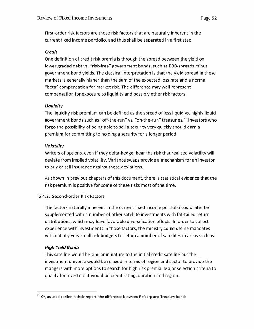
Review of Fixed Income Investments Page 52
First-order risk factors are those risk factors that are naturally inherent in the current fixed income portfolio, and thus shall be separated in a first step.
Credit One definition of credit risk premia is through the spread between the yield on lower graded debt vs. “risk-free” government bonds, such as BBB-spreads minus government bond yields. The classical interpretation is that the yield spread in these markets is generally higher than the sum of the expected loss rate and a normal “beta” compensation for market risk. The difference may well represent compensation for exposure to liquidity and possibly other risk factors.
Liquidity The liquidity risk premium can be defined as the spread of less liquid vs. highly liquid government bonds such as “off-the-run” vs. “on-the-run” treasuries.25
Volatility
Investors who forgo the possibility of being able to sell a security very quickly should earn a premium for committing to holding a security for a longer period.
Writers of options, even if they delta-hedge, bear the risk that realised volatility will deviate from implied volatility. Variance swaps provide a mechanism for an investor to buy or sell insurance against these deviations.
As shown in previous chapters of this document, there is statistical evidence that the risk premium is positive for some of these risks most of the time.
5.4.2. Second-order Risk Factors
The factors naturally inherent in the current fixed income portfolio could later be supplemented with a number of other satellite investments with fat-tailed return distributions, which may have favorable diversification effects. In order to collect experience with investments in those factors, the ministry could define mandates with initially very small risk budgets to set up a number of satellites in areas such as:
High Yield Bonds This satellite would be similar in nature to the initial credit satellite but the investment universe would be relaxed in terms of region and sector to provide the mangers with more options to search for high risk premia. Major selection criteria to qualify for investment would be credit rating, duration and region.
25 Or, as used earlier in their report, the difference between Refcorp and Treasury bonds.

Review of Fixed Income Investments Page 53
Emerging Market Bonds The logic here is the same as for high yield bonds, but based on high-yielding sovereign bonds from governments with significant credit risk.
Structured Finance Instruments This satellite would include structured products that might be highly illiquid but potentially “undervalued”. This would require extensive analysis and due diligence on such structures.
Insurance-linked Products such as “Cat Bonds” Given its tremendous risk bearing capacity, The Fund might be an ideal buyer of catastrophe- and reinsurance risk which would thereby diversify its investment risk (i.e., by assuming risk with very little correlation to financial markets such as earthquake risk). Realistically, a way to access this risk premium might be through an insurance tranche of structured products that are directly tailored for the Fund rather than through investments into readily available Catastrophe Bonds.

Review of Fixed Income Investments Page 54
6. Management Model
In this section we outline a proposal for an updated management model, suggest a division of responsibilities between the five key stakeholders, and reflect on the key parameters to be explicitly formulated in the NMoF’s mandate to Norges Bank, and what needs to be specified by Norges Bank.
Our suggested approach is an extension of the framework that was recently introduced by the NMoF that already implements various improvements in the areas of risk management and transparency. Particularly, Norges Bank is mandated to identify all relevant market risks and perform a return analysis of several systemic risk factors. Furthermore, specific limits for risks that are not well captured by the tracking error approach, for instance credit and liquidity risk, are introduced.
These changes are thus unquestionably in the spirit of our proposal and have the effect of improving transparency. Our proposed management mandate goes a step further by institutionalising a split between core assets and satellite risks that parallels the dual objectives of the fixed income portfolio. This has the benefit of a clear delineation of individual risk factors and adds an incentive to consciously select risk factors that can be managed within satellites. Thus, the result is not only transparency but hopefully also better performance with improved risk control.
6.1. Current Setup
The process of regulation, development, implementation and supervision encompasses five different instances. In short, the NMoF has the function of setting the general framework and guiding principles, the Executive Board of Norges Bank details the processes and standards within this framework, NBIM is in charge of the execution and can mandate internal and external managers.

Review of Fixed Income Investments Page 55
6.2. Proposed Scheme: Formulation of the Mandate
Stortinget The Parliament mandates the NMoF to elaborate a comprehensive strategy and approves the general framework.
Ministry of Finance The Ministry of Finance will formulate the mandate to the Norges Bank. The mandate should explicitly contain
• the general core-satellite framework (as described in this document),
• the suggested method for risk management
• the general risk management and reporting principles (disclosure)
For the core portfolio, this shall include
• A modified benchmark that suits the multiple objectives of the fund, with the goal of minimising its tracking error

Review of Fixed Income Investments Page 56
• Qualification criteria for core assets
For the satellite, this shall include guiding principles regarding general risk tolerance and rules:
• A maximum absolute risk budget for satellite assets defined as a function of risk tolerance and investment horizon. A comprehensive discussion of how to determine the optimal metric to define the risk budget would go beyond the scope of this report, but we will briefly mention possible approaches in chapter 7.3.
• A long term return target, or benchmark, defined as an absolute return above a risk-free rate, for the overall satellite portfolio
• A maximum level of deviation permissible from that benchmark in the interim under the assumption of severe stress events
• Possibly, a list of permissible “pure risk factors” or satellite assets, that could be grouped into "first order" satellites, already present in the current portfolio, and "second order satellites", that leverage the Fund’s risk bearing capacity and provide additional diversification
• Alternatively, a list of criteria that satellites need to fulfill, which leaves discretion regarding detailed specifications to the Executive Board of Norges Bank
The NMoF mandate to NBIM will thus only differentiate between core and non-core, i.e. assume one satellite. However the mandate shall give guidance as to how the non-core part is to be split into separate satellites by NBIM about its risk exposures and how satellites are opened and closed.
Executive Board of Norges Bank The NMoF delegates to the Executive Board the elaboration of definitions within the guidelines established:
The Executive Board designs a mechanism to mandate
• A dedicated (probably internal) instance directly responsible for the overall top down allocation and risk management
• Internal and/or external portfolio managers for the individual core and satellite mandates

Review of Fixed Income Investments Page 57
The Executive Board defines procedures for the measurement and management of risk
• at a portfolio level (the combination of satellites and core);
• at the level of the mandates assigned to the individual core and satellite managers;
and
• risk shall be estimated by means of different methods for normal and stress scenarios and shall include historical and forward-looking components.
For the core portfolio, the Executive Board shall
• Define criteria to select the core assets that qualify under the guidelines established by the NMoF
• Specify responsibilities, monitoring and risk management mechanisms
For the satellite portfolio, the Executive Board shall, in line with the overall framework and risk budgets defined by NMoF
• Define the “real world risk factors” within the permissible scope
• Define the allocation of those risk factors to the individual satellite portfolios
• Individually determine the benchmarks, management mechanisms and possible additional risk budgets for those satellites
• Develop a set of rules for the allocation of risk budgets
• Decide on the closure of a satellite or approve the opening of additional satellites at any point and define (absolute or relative) return targets for each new satellite
Norges Bank Investment Management The NBIM shall be responsible for
• The allocation of the total core portfolio (as defined by the Executive Board) to one or more core managers.
• The allocation of the total risk factor budget (as defined by the Executive Board) to one or more satellite managers.

Review of Fixed Income Investments Page 58
• The review of the allocation (to be done frequently, at least on a monthly basis).
• Performance measurement and control of individual managers, ensuring that at no point in time are there violations of risk budgets, other limit breaches or violations of allocation targets.
Internal and External Managers The appointed satellite managers
• Have full responsibility for their risks in accordance with the risk budgets and allocation targets.
• Shall act as centers of competence for the risks of responsibility, i.e., they are to perform detailed research, risk analysis, and develop action plans for any scenario in the fat tail region.
• They shall perform feasibility studies, paying particular regard, given the size of the institution, to market impact, and they shall devise systematic mechanisms to implement the allocation in order to use risk targets as effectively as possible and systematise risk management. These shall be submitted to and reviewed by the NBIM and the Executive Board.
6.3. Proposed Scheme: Challenges
In chapter 3 we have addressed some of the challenges in moving towards to this new framework. Notably, it has proven difficult to measure exposure to satellite risk factors. It is, in some instances, hard to find publicly-available and tradable indices for the various factors, and it may be difficult to separate the various factors from each other.
Measuring Exposure to Risk Factors The effort to separate the risk factors in a fixed income portfolio reveals the following challenges: Some instruments have components of different individual risk factors, others could be theoretically classified into different categories. For instance, it could already be argued that an AAA corporate bond is “riskier” (i.e. in terms of default risk) than an AAA government bond. Strictly speaking it could therefore be a satellite asset, although the markets may judge either the AAA corporate bond or the AAA government bond “safer”, meaning that the AAA corporate-over-government risk premium may be positive or negative. Often one

Review of Fixed Income Investments Page 59
would argue that AAA government and AAA corporate bonds are both core assets as they both fulfill typical “safety” and liquidity requirements.
Separating Risk Factors While some market risk factors can clearly be separated from one another, for example interest rate volatility from interest rate “level” risk, and others such as interest rate and earth quake insurance risks might even seem independent, many risk factors are inherently correlated and often difficult to separate. In particular the risk factor “liquidity” is difficult to separate from risk types such as “credit” or “high yield” risk as pointed out in section 3.
Finding publicly-available Benchmarks Public benchmarks are either not available at all, or, where they are available, often not liquid enough and thus in practice impossible to track for a fund as large as the GPF.
Indeed compromises are inevitable when addressing the above mentioned issues and a conservative but pragmatic set of rules for core/satellite asset selection needs to be developed. The different components of the current portfolio need be analyzed thoroughly, and if an asset class does not qualify this could be an indicator that it may contain opaque risks and should be removed. A satisfactory definition of a benchmark for an overall satellite might be difficult to find, so an absolute return target would then be an alternative.
6.4. Proposed Scheme: Benefits
Transparency, Accountability and clear Incentives The first and obvious benefit is that risk can be measured, and yield attributed to each satellite as well as to the core portfolio. Each manager has a clearly defined objective for which he is fully accountable.
Less obviously, the benefit of the core satellite approach is that it allows the - potentially competing - dual objectives of preserving wealth in times of crisis and generating income by taking some specific risks to be satisfied. The proposed scheme separates the two objectives and sets distinct incentives in accordance with the distinct nature of both objectives.

Review of Fixed Income Investments Page 60
We will elaborate this point in 8.1, but it should already be stated here that the proposed structure ensures that portfolio managers have no incentive to take undesirable risks.
Reduction of Fat Tail Risks The NMoF is directly in charge of setting the maximum risk budget for the overall satellite portfolio. Thus, there should be no significant underperformance in the sense that "hidden" risks suddenly surface beyond what is defined as risk tolerance by the NMoF.
In a core satellite approach, the risks would clearly be limited to the maximum risk level as defined by the NMoF, whereas in the current setup the actual risk can reach levels that are not tolerable.
Better Risk Reward Characteristics Firstly, the core satellite approach allows a clear analysis of which risks are worth taking in the long run and which are not, as well as an analysis of the benefits of low correlation between individual risks. Therefore, a core satellite approach introduces a “competitive element” between risk factors and the incentive scheme supports an efficient selection. As a result, the quality of the risks will tend to improve which is likely to lead to better performance.
Secondly, the satellite portfolio allows for the flexible addition of new, potentially better-diversified risks. At a future time this might include insurance-linked products that would ideally leverage the risk bearing capacity of the Fund.
As a result, the core satellite approach has the potential to both improve the performance and decrease the risk of the portfolio.

Review of Fixed Income Investments Page 61
7. Risk Budgeting and Asset Rebalancing
7.1. Asset Rebalancing between the Fixed Income Core and Risk Assets
As long as oil revenues provide large cash inflows to the Fund, the investment horizon is in principle “indefinite” and rebalancing can to a large extent be performed indirectly through directed allocation of new revenues. As pointed out in section 2 of this report, the core fixed income portfolio reduces the overall volatility of the Fund. This is particularly true in times of stress. Both the equity allocation and the satellite Fixed Income assets have the function of generating additional income beyond the "risk free return".
For the allocation between fixed income core and satellite assets the following options are possible:
• Fixed allocation, determined by the NMoF. Rebalancing occurs only as a function of value changes, which means that risky assets are bought when they get cheaper and sold when they get more expensive. Even though in practice this will occur with a certain lag, as a function of the rebalancing frequency and execution procedures, this can be described as acyclical. It excludes any discretion by the portfolio manager.
• Flexible allocation determined by a fixed rule set, which is designed by the NMoF. The rule set allows for the setting of additional (counter-)cyclical elements by systematically buying equities after falls and decreasing risky asset exposure after long periods of benign markets, while excluding any discretion. The question of whether outperformance (or to put it differently “improved asset protection”) can be generated by such a rule needs to be tested separately, but ruling out discretion gives protection from behavioral biases.
• The NMoF determines strategic allocation bands with room for “tactical adjustments” by NBIM. This allows for marginal discretionary or systematic adjustments within the bands.
• Flexible allocation based on decisions by NBIM.
In any case, large adjustments are not realistic as the volume is too large to rebalance frequently. Thus the current allocation between equities, fixed income

Review of Fixed Income Investments Page 62
and real estate has been set as fixed, and (customized version of) the BGAI has been selected as the benchmark for the bond portfolio. Within the narrow bandwidth that would be practically feasible we would favor a systematic approach because
• It is suggested by research and experience that systematic strategies tend to produce better results in the long run than human discretion,
• It can be more easily explained to parliament,
• It is transparent and results are replicable,
• And last but not least it discourages taking opaque risks.
There are indeed various possible rebalancing rules:
Simply keeping the 60% / 35% / 5% split constant has a contrarian component and is countercyclical to “typical fund behaviour”, as the Fund would sell performing assets (say equities in case of an equity rally) to invest in underperforming assets (i.e., fixed income).
7.2. Risk Allocation at the Portfolio Level
The starting point is the target risk allocation between the core and specific satellites as defined by the NMoF on a macro level and specified by the Executive Board of Norges Bank (cf. chapter 6).
The typical investment fund management strategy would attempt to increase the percentage allocation to safe government bonds (i.e. to the core) in times of uncertain market situations and in particular during a crisis, while increasing the allocation to risk-bearing investments (i.e. to satellites) when conditions are improving, early in an expansion cycle.
On the other hand a fixed allocation rule between core and satellite (as for the allocation between equity, fixed income and property investments) could have the opposite effect: a satellite portfolio that had declined in value would trigger further investments financed by potential gains (or relatively weaker losses) of the core portfolio. Clearly this strategy is risky even though not necessarily bad given the risk-bearing capacity of the Fund.

Review of Fixed Income Investments Page 63
We therefore suggest that the updated management model will have a fixed limit of total satellite risk tolerance but not necessarily a fixed allocation rule between fixed income core and satellite.
However, the updated GPF mandate might differentiate between declines in the prices of individual investments that trigger a transfer from the core to a satellite according to the selection criteria of such assets, and a global crisis situation that would allow the keeping of those assets within the core in order to avoid excessive disturbance to the management process.
7.3. Definition of Risk Budgets and Asset Rebalancing within Satellites
Here we outline a number of approaches that might serve as a reference in defining the right risk metric as a basis for allocation rules. They are not mutually exclusive, and taking into account the very different nature of some satellite risks, the mandate should provide the flexibility to define risk in the most appropriate way for each satellite.
Discretionary Allocation based on Maximum Risk Tolerance
Asset allocation in the satellites will, as a first step, be defined as a function of the total portfolio risk tolerance and investment horizon. Once the total risk tolerance is defined, the rebalancing of risks between satellites could be simply delegated to NBIM. NBIM could then decide on a discretionary basis in a top-down manner to increase or decrease particular exposures of or within individual satellites such that diversification benefits can be optimised while target risk exposures can be maintained.
However, if the NMoF wants to define a scheme for risk budgeting more specifically, risk limits will likely have to be set either as maximum expected drawdown in a static exposure, over volatility targets, or as a combination of the two.
Volatility or Value at Risk Target
The volatility target can be defined as a maximum absolute volatility target or as the marginal contribution to volatility in a portfolio context. Defining an absolute volatility / VaR (or Expected Shortfall) target for satellites means that allocations

Review of Fixed Income Investments Page 64
are divided by a volatility measure as soon as the volatility measure crosses the previously defined maximum acceptable limit.
Provided a reasonably reliable indicator for implied volatility is available, this thus proactively reduces risk when crisis scenarios become more likely and allows the fund to benefit optimally from its risk-taking capacity: Reduce exposure when risk is high, increase exposure when risk is low.
The volatility target approach is only sensible for the more liquid types of risks that have a clear correlation with financial cycles, for instance high yield bonds or emerging markets bonds.
Static Exposure
For any other asset, particularly the illiquid and more exotic satellites, or where the benefits of a volatility target cannot clearly be proven, setting a static limit to exposure may be the best option. For instance, in the case of selling insurance a static exposure is probably the ideal solution as there is no implicit correlation with financial cycles and risk premia might be significant, particularly in periods following insurance events.
Of course, such static exposures imply that a mechanism to respond to drawdowns is not required and thus mark-to-market drawdowns have to be "sat through". By design, this has a countercyclical feature that tries to exploit the time-varying perception of risk by "writing insurance when the premium is high". As a result, risk needs to be defined as a maximum possible drawdown using methods such as stress testing and modeling on the basis of historic events, so rebalancing between satellites for such categories will be minimal.
“Pure Alpha” Approach
In a “pure alpha” approach risk is defined as the total investment amount. For most assets, it is probable that there are more precise risk metrics. For some exotic risks however such as cat bonds, if there is evidence that they produce superior returns in the long term but no immediate way to measure the expected shortfall or other risk measures due to the non-availability of data, the “pure alpha” approach might be the only valid option to measure risk.

Review of Fixed Income Investments Page 65
7.4. Risk Budgeting Approach and Allocation - Reviewing the Choices
Chapter 7.3 is provided as an illustration of possible mechanisms, and a comprehensive analysis would go beyond the scope of this report. We now quickly review the suitability of these mechanisms for the risks in the Fund.
Theoretically, a volatility-measure based approach has the advantage that it improves the exploitation of the risk-bearing capacity of the fund by dynamically adjusting the exposure to actual market risk. However, as became evident in the last chapter, the availability of choices mainly depends on whether the assets in question are sufficiently liquid to permit dynamic risk management, and whether there is clear evidence that this actually produces a benefit for the Fund in the long run when transaction costs are factored in. Otherwise a static exposure, where risk is defined as maximum drawdown, is the best practical option.
Of course, volatility targets do not only require enough liquidity, but are also feasible only if a leading implied volatility indicator is available. For GPF satellites, volatility / VaR targets would need to be defined very carefully in order to avoid frequent reallocations which would lead to significant trading costs.
Applying this scheme to a few selected satellite assets, one might come up with the following definition of risk budget approaches (for illustrative purposes only):
Risk type (example) LiquidityAvailability of leading implied vol measure
Risk budgeting approach
Risk definition
Credit highoption markets, implied CDS volatilities
volatility target or VaR
absolute amount dynamically manageable via volatility target
Emerging markets bonds
relatively high
implied CDS volatilitiesvolatility target or VaR or static appr.
absolute amount dynamically manageable via volatility target
Structured Finance lownot practicable even if maybe theoretically possible
static risk budgetmtm drawdown in worst case scenario such as multiple default
Insurance, Cat Bonds very low none static risk budgetmtm drawdown in worst case scenario such as California earthquake

Review of Fixed Income Investments Page 66
8. Benchmark Construction
The construction of the benchmark is a very delicate task which has multiple objectives. The primary goal of this chapter is to show that the benchmarks for core and satellite tranches need to be formulated very differently as a result of their different objectives, and that we believe a proprietary set of benchmarks would likely serve the purpose better than any publicly-available benchmark.
The proposals below should be seen as explorative. Further research is required to define solid benchmarks for both core and satellites.
In our case the benchmark needs to satisfy the following criteria
• Fulfill the basic function of implementing the desired asset allocation
• Act as a valid risk management tool
• Set the right incentives for the portfolio managers
More specifically, the GPF may require some additional filters in the light of its long term horizon and sheer size.
• The size may require a benchmark system that incentivises low portfolio turnover to minimize slippage and market impact while still enabling hedging in periods of stress
• Optimize the risk-taking capacity
8.1. Benchmarks are Incentive Schemes
As noted in 6.3, a particular benefit of the core satellite approach is that it allows the incentives to be set distinctly according to the dual objectives of the fixed income portfolio, i.e. preserving wealth in times of crisis and generating income by taking some specific risks. Particular emphasis should be placed on setting the right incentives to ensure an alignment of the interests of all stakeholders with the overall interests of the Fund.
One of the main objectives of the core satellite approach is indeed to ensure that all stakeholders are remunerated for achieving clear targets that support the long-term growth of the Fund.

Review of Fixed Income Investments Page 67
• The objective for the core portfolio managers is to track the benchmark. This requires a tracking error target of as close as practically possible to zero. How close depends on each individual market, but the core managers should only be allowed a minimum tracking error and this only for the reason of improving the efficiency of implementation. Portfolio managers should not have any incentive to include opaque risks in their portfolio, nor should they have any incentive to try to improve the performance of the portfolio. The current objective of the core portfolio is to act as a safety cushion in times of crisis. Should the NMoF change/extend this objective, the benchmark must be reviewed accordingly.
• The satellite portfolio managers should be rewarded for their capacity to use their risk budget as effectively as possible. A long-term metric along the lines of absolute return versus the risk budget should be used to incentivize the manager to distinguish “most profitable” investments given the same level of risk, or to minimize costs. Periodical audits should make sure that the manager complies with the asset restrictions defined in the mandate. This should not be connected to the size of their assets, as the allocation to the satellites can vary according to their allocated risk budgets. Even if the allocation factor at some point is close to zero, the manager should have the same incentives as a manager who is responsible for a significantly larger exposure to another risk type.
• Since the Fund has a very long-term perspective, the incentive system should also have a very long time horizon (at least over one full business cycle) to avoid the possibility that a stakeholder might take short-term decisions at the expense of the long-term objective. The incentive system needs to be formulated both for Norges Bank, being responsible for the overall macro management of the portfolio, and for individual managers. Remuneration needs to be linked to adherence to the defined targets, while a fully transparent system of penalties needs to be defined for breaches of the risk budgets or scope of mandated assets.

Review of Fixed Income Investments Page 68
8.2. Benchmark Construction - Available Options
In practice, investors have a choice between standard publicly-available indices calculated by Investment Banks and based partly on Ratings, or constructing their own proprietary benchmarks.
Publicly-available Indices As opposed to equity indices, an institutional fixed income investor may find the availability of public benchmarks that suit its objectives limited.
As described in chapter 2.1.ff, the existing benchmark BGAI aims to cover the fixed income sector very broadly. It will not be adequate for the purpose of the new core & satellite set-up because it includes a variety of types of debt security and thus mixes core and satellite objectives.
Rating Agencies Ratings provided by rating agencies may provide useful guidance for selection of FI instruments in good times. However, their limitations have been amply demonstrated during the crisis when the quality of ratings for some instruments – in particular, structured credit – was much lower than expected. Also, and importantly for investors, adjustments in ratings have been shown to lag significantly behind the market’s perception of default risk.
Proprietary Benchmarks The construction of proprietary benchmarks is thus often the best (and sometimes the only valid) option, in particular for large funds. This may include some dependence on ratings and even public benchmarks, but it needs to allow for the possibility of bespoke components. To make up for the possible loss of transparency from using internal benchmarks, these need to be calculated by a fully independent external party.
8.3. Market-implied Benchmarks
In contrast to ratings by major agencies markets typically respond to increasing risk perception much more quickly. The advent of markets that price default risks (through CDS and similar instruments) is relatively recent. However we think that it provides guidance and information that should not be overlooked and that is highly relevant. We therefore propose using market-implied ratings as a complement to traditional benchmarks.

Review of Fixed Income Investments Page 69
Alternatively, the quality of bonds may be determined in a traditional way through the credit agencies ratings, e.g., one could decide that only an AAA rating by one of the leading agencies qualifies for the core. To make sure that the portfolio managers stay ahead of the curve, the NMoF could set guidelines requiring the NBIM to monitor the volatility of default spreads, and if there were unusual volatility in one issue, benchmarks would reflect these adjustments.
This is further explored in an example below.
8.4. Core Portfolio Benchmark
The Role of the Core Portfolio The fixed income (FI) component of the Fund has a number of key functions. Some of these have been discussed earlier in the report but we reiterate them here for the sake of clarity.
First, the FI portfolio should moderate the overall level of risk in the Fund (because it has lower volatility than does equity). Second, the FI component must provide sufficient liquidity to allow the fund to rebalance in times of stress. Third, the FI component has the potential to act as a (partial) hedge for the future cash outflows in the fund. Fourth, as with the equity component, it is a vehicle through which the Fund’s owners can express their risk preferences in order to earn risk premia.
These are the main functions of the FI component. In order for these functions to be realised it is important that the performance and risk exposure of the fund be “monitorable”. This means that the rules determining the composition of the benchmark portfolio must be transparent, i.e. the benchmark must, at all times, be both theoretically replicable and practically both replicable and investable by an external party.
These issues are common to most long-term investment portfolios. However, in this report we propose (i) separating the FI portfolio into a core portfolio and one or more satellite portfolios, and (ii) locating essentially all long-left-tail risks in the satellites. These long-tailed risks include liquidity and volatility risk and, perhaps, a part of the risk associated with high yield debt. The core FI portfolio should not have significant exposure to these long-left-tailed risks.
The types of instrument that should be included in the core in order to provide (i) risk moderation at the overall portfolio level, (ii) liquidity (to allow rebalancing)

Review of Fixed Income Investments Page 70
and (iii) cash flow hedging are high-grade government debt, government-related debt, high-grade corporates and high-grade securitised debt. This list overlaps very substantially with the types of instrument in the current BGAI (and, therefore, with the Fund’s current FI benchmark). What may well be different in the Fund’s core portfolio is the maturity profile.
Maturity Profile of the Core Portfolio The analysis presented earlier in this report reveals two results that are relevant to the question of the maturity profile of the core portfolio. The first is the factor structure, i.e., that returns in government bond markets are well described by two factors, the level and the slope of the yield curve. Moreover, apart from very short-term bonds, the level factor is dominant (in terms of the R-squared) and choosing among alterative portfolios is effectively the same as choosing the degree of exposure to the level factor (i.e., choosing the duration).
The second result is the absence of convincing evidence of a long-run risk premium for bearing yield curve risk and, without a risk premium, the only reason to take on exposure to the level of interest rates is if it acts as a hedge.
Regional and Currency Distribution The currency of an issue determines the particular yield curve to which the issue is exposed (US dollar, Yen etc.). The country of an issue determines its exposure to sovereign risk. Currency exposure and sovereign exposure can be managed independently. However, sovereign risk and currency risk are likely to be correlated: if country X defaults then its currency is likely to weaken. Currency exposure and country exposure need to be determined jointly.
The Current Benchmark The current benchmark meets at least some of the requirements outlined above. It consists substantially (around two thirds) of high quality government or government-related bonds and is therefore likely to help to lower the overall risk of the portfolio and provide good liquidity in all but the most extreme conditions.
On the other hand, the quasi-market weights of the BGAI serve no particular purpose apart from creating a very wide spread of holdings. Similarly, because the maturity profile of the BGAI is, effectively, just what happens to have been issued at a point in time, the degree of interest rate exposure in the benchmark has no connection with any of the parameters that define the “purpose” of the Fund such as the timing and risk characteristics of the Fund outflows.

Review of Fixed Income Investments Page 71
Redefining the Benchmark These two areas, the weighting pattern across issues and the maturity profile, are ones that could be usefully addressed in redefining the benchmark. The maturity profile is particularly important, and also difficult to resolve. To improve the liquidity of the fund it might make sense to reduce the average maturity and include bonds with less than one year to maturity. This would also lower the rate of return volatility and so improve the likelihood that the fund would be able to rebalance in a crisis. The other considerations here are the risk characteristics of the Fund’s outflows.
The distribution of the benchmark across countries requires an analysis of their default risks. Sovereign default is a left-tail event and, while the probability of the default of a major country may be small, it is probably to be taken more seriously than it would have been five or ten years ago.
Finally, a positive feature of the current benchmark is that it is investable, observable and easily measureable. The new benchmark must maintain these qualities but it needs to focus on core assets only and limit tracking error to the minimum consistent with efficient replication.
8.5. Satellite Setup Processes and Benchmark Definition
Benchmark setting at the satellite level is a relatively complex issue and the design process needs to involve all stakeholders. As opposed to the core benchmark, which needs to be highly liquid and easily replicable, the framework for setting the satellite benchmark needs to be flexible enough to account for the multifaceted nature of satellite risks, while institutionalising a clear framework that a) ensures that the total risk is controlled and limited; b) restricts and defines the scope of risks held by individual satellite managers and ensures uncontrolled risk-taking behaviour is avoided while c) delegating the actual formulation of the strategy to the NBIM / the managers.
The benchmark-setting exercise for satellites is thus most likely a two-level process in which a) a long term return target is estimated and b) individual satellite benchmarks may be formulated. The long-term return target needs to be estimated and formulated by the NMoF as it will serve as an exclusion criterion for the establishment of any new satellite. The individual benchmarks need not necessarily be defined by the NMoF; in principle, they could be formulated by

Review of Fixed Income Investments Page 72
other stakeholders. This ensures that satellites are set up to harvest high long-term risk premia in a competitive way rather than simply taking fat-tailed risks.
At this stage, two distinct approaches to benchmark formulation, or a hybrid of the two, are possible. It might serve the reader's understanding to illustrate the process, by means of two examples - high yield government bond/emerging markets bonds and volatility/insurance.
8.5.1. Standard Approach: Top-Down Benchmark Definition
Step 1: Target Return Estimate A long-term target return estimate for certain products or risk factors will likely serve as a trigger to request an investment mandate for a new product class. In case the risk factors are not already part of the NMoF approved “risk factor universe”, NMoF must approve the overall risk type and possibly specify an overall limit for such risk.
Step 2: Risk Return Analysis Prior to setting up a satellite, a risk/return analysis including an analysis of risk premia as outlined in chapter 3.7 is performed for each satellite candidate. If the results indicate that such an investment is beneficial in the long term, a satellite can be set up. “Beneficial” could mean that the target return per risk unit is high, diversification benefits are significant or a combination of the two.
Step 3: Definition of Benchmark Portfolio Once a satellite is approved, a benchmark portfolio will be defined to help specify typical instruments. Indeed, as the characteristics of individual satellites may be very different, flexibility to tailor these benchmark portfolios to each satellite is necessary. In some instances publicly-available indices might be used as a reference. The benchmark system for classical higher-yielding fixed income instruments, such as high-yield corporate or emerging markets bonds etc. could be based on either an appropriate publicly-available index, rating brackets, or default spread volatility. Where no valid benchmarks can be defined, as might be the case for insurance or volatility, absolute targets might be used.
Step 3: Definition of Risk Characteristics In order to determine the risk appetite for a satellite, the relevant risk characteristics need to be defined. Possible options are outlined in section 7.3.

Review of Fixed Income Investments Page 73
Step 4: Drawdown Limits NBIM will need to define limits for these risks and an overall stress-draw-down-limit for the satellite. Managers would be incentivised to hold a portfolio only if it has the same characteristics as the benchmark.
Satellite Benchmark Construction - Example High Yield / Emerging Markets This will be illustrated with the example of the high-yield government bond and/or emerging market bond satellites.
The risk return analysis serves as ex-ante criterion of investment characteristics, e.g., evidence that the satellites can produce returns in excess of the long-term target or provide desirable diversification effects shall be produced before the satellite is set up.
A benchmark is then to be defined. For example, for bond markets it would possibly include:
• Credit type
• Credit quality
• Credit duration
• Maturity
• Region
These parameters must be chosen in line with the specific targets. In the case of high-yield and emerging markets there are a handful of reasonable indices available that can be tracked. It might thus be considered sufficient to use an index such as the Barclays High Yield Index or the JPMorgan Emerging Market Bond Index (EMBI) as a flexible benchmark.
Alternatively, the satellites may encompass different brackets of risk tranches as priced by the market. Tranches could be defined as follows:
Definition, Implied Risk Absolute Benchmark Relative Benchmark
Core <80 None Target Portfolio Core
Low Risk Satellite 80 to 150 LIBOR + XX% Target Portfolio 80/150
High Yield Satellite 150 to 300 LIBOR + XX% + YY% Target Portfolio 150/300
Junk Satellite 300 to 600 LIBOR + XX% + YY%+ ZZ% Target Portfolio high riskIn basis points p.a.

Review of Fixed Income Investments Page 74
For illustrative purposes, at current implied rates, the following bond issuers would constitute, amongst others, these benchmarks:
Issuer 5Yr CDSSweden 33.84Finland 37.46Switzerland 46.51USA 46.69Germany 53.17Australia 53.5United Kingdom 60.92Japan 77.09Malaysia 80.87Chile 83.08Austria 85.54France 89.7Thailand 116.76Brazil 120.28Indonesia 156.07Turkey 169.97Italy 175Vietnam 378.74Dubai 402.6Portugal 440Argentina 613.53Greece 845.83
In basis points p.a.
Source: Bloomberg
The only incentives for managers would be to replicate the target portfolio. It is important that "replicating" does not mean "minimising the tracking error" but investing in a portfolio “with very similar characteristics” and, in particular, without exposure to other risk factors.
8.5.2. Alternative Approach: Absolute Target
Whenever it is not possible to find an appropriate benchmark, the following approach might be chosen, once NMoF has approved the risk category and overall risk appetite as mentioned above:
Step 1: Target Return Estimate A long-term target return estimate is proposed or agreed by the NBIM Executive Board.
Step 2: Complementary Benchmarks The NBIM Executive Board could either define a maximum risk exposure for the satellite or per risk class (as discussed in chapter 7.3.).

Review of Fixed Income Investments Page 75
Step 3: Definition of Risk Characteristics In order to determine the risk appetite for this satellite, the relevant risk characteristics will be defined; possible options are outlined under chapter 7.3. Possibly the NBIM Executive Board would define maximum drawdown limits for pre-defined stress scenarios.
Satellite Benchmark Construction - Example Volatility / Insurance With reference to another example that was described in more detail earlier, we consider the volatility satellite. This discussion should also be valid for other satellites that could also be considered as "sellers of insurance".
Firstly, the targeted average long run rate of return over risk-free assets will serve as a long-term benchmark and criterion for investment possibility.
Again, if no relative benchmark is defined, the risk budget is sufficient to limit the risk a manager can take, while theoretically he has many options for the implementation of the strategy. For instance, he could choose to sell options, or take positions in VIX futures or Variance Swaps.
If a shorter-term relative benchmark were chosen, the parameters that must be set to construct a benchmark would consist of the following features:
• Type of assets permitted
• Maximum shortfall as a percentage of the total notional exposure
• Maturity
• Regional focus
These examples are purely illustrative. It would require extensive research to find an exhaustive list of parameters to be considered and for risk levels to be set. A comprehensive discussion of benchmark setting would go beyond the scope of this report.

Review of Fixed Income Investments Page 76
9. Conclusion and Outlook
This report proposes a new framework designed to improve the Fund’s structural capability to control risks and deal with crises. It also institutionalizes mechanisms to reduce drawdowns in such events while optimising its risk-taking potential in normal markets.
The fixed income portfolio has two – possibly competing – objectives: (i) preserving wealth in times of crisis and (ii) generating income by taking exposure to risks such as liquidity, credit and volatility. In the current setup these dual objectives are reflected, on the one hand, by targeting a passive benchmark and, on the other hand, by allowing the portfolio manager to generate “alpha” within a certain tolerance band.
This study discusses the possibility of separating these two objectives and suggests the implementation of a core and satellite approach. We argue that managing the portfolio along such lines would lead, first of all, to increased transparency by attributing the performance to risk factors wherever possible.
A core-satellite approach would facilitate the separation of the two different principal functions of the fixed income portfolio – reducing volatility and providing liquidity on one hand and, on the other, using the fund’s risk-bearing capacity to exploit certain risk premia inherent in fixed income markets.
This would make it possible to formulate separate mandates according to the distinct requirements of the two functions and to define incentive structures in line with the particular requirements of the dual objectives.
Core managers should focus on benchmark tracking, while satellite managers should be rewarded for the efficient use of their risk budgets. This would create positive competition between the possible risk factors, improving the overall performance of the fund while decreasing the overall risk.
The benefit of the core-satellite approach is thus to be seen not only in increased transparency, but in the possibility of a more favourable risk-reward profile for the fund. The NMoF will also be able to directly set and control the maximum allowable risk for non-standard fixed income risk factors.
We have also outlined in an “updated management model” for how the NMoF mandate could be formulated and how the responsibilities, delegation of powers and reporting lines for the five primary stakeholders could be separated.

Review of Fixed Income Investments Page 77
Of course, some aspects relevant to the implementation of the core-satellite model were only very briefly touched upon in this report. One question is the design of the allocation mechanisms between the risky satellites and the safe core portfolio. Another question is the definition of benchmarks, which needs to be done carefully for both the core and satellite, and probably individually for each satellite.
The development of specific allocation mechanisms and the formulation of individual satellite benchmarks require further research and are outside the scope of this document.
Review of Fixed Income Investments Page 78
References
Amihud, Yakov, Haim Mendelson and Lasse Heje Pedersen, “Liquidity and Asset Prices”, Foundations and Trends in Finance, Vol 1, No 4, pp 270 - 364 Baele, Lieven, Geert Bekaert and Koen Inghelbrecht, 2007, “The Determinants of Stock and Bond Return Movements”, National Bank of Belgium working paper research Bakshi, Gurdip and Nikunj Kapadia, 2003, “Delta-Hedged Gains and the Negative Market Volatility Risk Premium”, The Review of Financial Studies, Vol 16, No 2, pp 527-566 Boland, Vincent D., Guy Sanderson, Rachel TettDillian, “An exposed Position”, Financial Times, March 9 , 2010 Bollerslev, Tim and Hao Zhou, 2006, “Expected Stock Returns and Variance Risk Premia”, Finance and Economics Discussion Series, Federal Reserve Board, Washington D.C. ___________ , George Tauchen and Hao Zhou, 2008, “Expected Stock Returns and Variance Risk Premia”, working paper Bolton, P and Federic Samama, “Contingent Capital & SWFs: A Natural Match”, October 2010. Presentation available at cgt.columbia.edu/files/papers/Patrick_Bolton_Powerpoint.pptx Bondarenko, Oleg, 2007, “Variance Trading and Market Price of Variance Risk”, working paper Bondarenko, Oleg, 2004, “Market Price of Variance Risk and Performance of Hedge Funds”, working paper Brown, David T. and William J. Marshall, 2001, “Assessing Fixed-Income Fund Manager Style and Performance from Historical Returns”, Journal of Fixed Income, pp 15-25 Campbell, John Y., Adi Sunderam and Luis M. Viceira, 2007, “Inflation Best or Deflation Hedges? - The Changing Risks of Nominal Bonds”, NBER Working paper Carr, Philip and Dilip Madan, 2002, “Towards a Theory of Volatility Trading”, working paper _________ and Liuren Wu, 2006, “A Tale of Two Indices”, Journal of Derivatives _________, 2008, “Variance Risk Premiums”, The Review of Financial Studies, Vol 22, No 3 ,pp 1311-1341

Review of Fixed Income Investments Page 79
Chen, Yong, Wayne Ferson and Helen Peters, 2010, “Measuring the timing ability and performance of bond mutual funds”, Journal of Financial Economics, Vol 98, pp 72-89 Cochrane, John H., and Monika Piazzesi, 2005, “Bond Risk Premia”, The American Economic Review, Vol 95, No.1, pp 138 -160 ____________ , (2008) “Decomposing the Yield Curve”, Working Paper. Available at SSRN: http://ssrn.com/abstract=1333274 Collin-Dufresne, Pierre, Robert S. Goldstein and J. Spencer Martin, 2001, “The Determinants of Credit Spread Changes”, Journal of Finance, Vol 56, No 6, pp 2177-2208 De Jong, Frank and Joost Driessen, 2006, “Liquidity Risk Premia in Corporate Bond Markets”, working paper Dick-Nielsen, Jens, Peter Feldhutter and David Lando, “Corporate Bond Liquidity Before and After the Onset of the Sub-prime Crisis”, MAARC meeting, Moody’s New York, October 27, 2010 Dimson, Elroy, Paul Marsh and Staunton , 2002, Triumph of the Optimists, Princeton University Press. Fama, Eugene F. and Kenneth French, 1993, “Common Risk Factors in the Returns on Stocks and Bonds”, Journal of Financial Economics, Vol 33, pp 3 - 56 ______________ and Robert R. Bliss , 1987, “ The Information in Long-Maturity Forward Rates”, The American Economic Review, Vol 77, No. 4, pp 680 - 692 Fung, William and David A. Hsieh, 2001, “Risk in Hedge Fund Strategies: Theory and Evidence from Trend Followers”, The Review of Financial Studies, Vol 14, No 2, pp 313-341 Hordahl, Peter, 2008, “The Inflation Risk Premium in the Term Structure of Interest Rates”, BIS Quarterly Review Huang, Jing-Zhi and Huang, Ming, 2003, “How Much of Corporate-Treasury Yield Spread Is Due to Credit Risk?: A New Calibration Approach”, Working paper. Available at SSRN: http://ssrn.com/abstract=307360 Krishnamurthy, Arvind, 2010, “ “How Debt Markets Have Malfunctioned in the Crisis”, Journal of Economic Perspectives, Vol 24, No 1, pp 3 – 28 Litterman, Bob & Scheinkman, José, 1991, Common Factors Affecting Bond Returns, Journal of Fixed Income (June) pp 54-61.

Review of Fixed Income Investments Page 80
Longstaff, Francis A., Jun Pan, Lasse H. Pedersen and Kenneth J. Singleton, (2007), “How Sovereign is Sovereign Credit Risk”, working paper. Rosenberg, Joshua V. and Samuel Maurer, 2008, “Signal or Noise? Implications of the Term Premium for Recession Forecasting”, Federal Reserve Bank of New York Economic Policy Review Schaefer, Stephen M. and Ilya Strebulaev, 2006, “Risk in Capital Structure Arbitrage”, working paper Schaefer, Stephen M. and Ilya Strebulaev, 2008, “Structural Models of Credit Risk are Useful: Evidence from Hedge ratios on Corporate Bonds”, Journal of Financial Economics, Vol. 90, pp. 1-19 . Sekkel, Rodrigo, 2011, “International Evidence on Bond Risk Premia”, Journal of Banking and Finance, Vol. 35, pp 174 - 181 Sengupta, Rajiv and Yun Man Tan, 2008, “The LIBOR-OIS Spread as a Summary Indicator”, Economic Synopses, Federal Reserve Bank of St Louis Wright, Jonathan H., 2008, “ Term Premiums and Inflation Uncertainty : Evidence from an International Panel Dataset”, Finance and Economics Discussion Series, Federal Reserve Board, Washington D.C.

Review of Fixed Income Investments Page 81
Figures

Review of Fixed Income Investments Page 82
Flight to Quality and Liquidity of Government Bonds
Figure 1
-Feb '80
Apr 74
Jun 74-Oct '08
-15%
-10%
-5%
0%
5%
10%
15%
-15% -10% -5% 0% 5% 10% 15%
BBB Return
Trea
s Re
turn
: Act
ual -
Pre
dict
ed
Oct '79
Source: Morningstar and authors’ calculations

Review of Fixed Income Investments Page 83
Figure 2
BGAI Historical Composition by Quality (MV%) – Trailing 5 Years*
Source: Barclays Capital

Review of Fixed Income Investments Page 84
Figure 3
REFCO – Treasury spread versus On-Off-the-run Treasury Spread
Comparison of liquidity proxies
0
20
40
60
80
100
120
140
160
Apr
-91
Apr
-92
Apr
-93
Apr
-94
Apr
-95
Apr
-96
Apr
-97
Apr
-98
Apr
-99
Apr
-00
Apr
-01
Apr
-02
Apr
-03
Apr
-04
Apr
-05
Apr
-06
Apr
-07
Apr
-08
Apr
-09
Apr
-10
bps
REFCO - Treasury spread
On-off the run treasury spread (AA data)
Source: Bloomberg and AGS report.

Review of Fixed Income Investments Page 85
Figure 4
Distribution & Correlation of Monthly Returns on FF Factors (1927-2010)
Monthly Excess Returns on SMB
0%
5%
10%
15%
20%
25%
30%
35%
-30 -26 -22 -18 -14 - 0 -6 -2 2 6 10 14 18 22 26
Monthly Excess Returns on Market
0%
5%
10%
15%
20%
25%
-30 -26 -22 -18 -14 -10 -6 -2 2 6 10 14 18 22 26
Monthly Excess Returns on HML
0%
5%
10%
15%
20%
25%
30%
35%
-30 -26 -22 -18 -14 -10 -6 -2 2 6 10 14 18 22 26
Monthly Excess Returns on MOM
0%
5%
10%
15%
20%
25%
30%
-30 -26 -22 -18 -14 -10 -6 -2 2 6 10 14 18 22 26
-20
-10
0
10
20
30
40
50
-40 -30 -20 -10 0 10 20 30 40 50
Rm - Rf
SMB
-60
-50
-40
-30
-20
-10
0
10
20
30
-30 -20 -10 0 10 20 30 40
HML
MO
M
Source: K. French website and author calculations

Review of Fixed Income Investments Page 86
Figure 5
VIX and Time Series Volatility (1990-2010)
0%
10%
20%
30%
40%
50%
60%
70%
80%
90%
Jan-90
Jan-91
Jan-92
Jan-93
Jan-94
Jan-95
Jan-96
Jan-97
Jan-98
Jan-99
Jan-00
Jan-01
Jan-02
Jan-03
Jan-04
Jan-05
Jan-06
Jan-07
Jan-08
Jan-09
Jan-10
Annualised Vol Times Series Vol
VIX
Source: CBOE and author calculations

Review of Fixed Income Investments Page 87
Figure 6
Returns to Variance Swaps
Panel (a) Log excess return
Log (VIX / Realised Vol.)
-100%
-50%
0%
50%
100%
150%
200%
250%
Jan-90
Jan-91
Jan-92
Jan-93
Jan-94
Jan-95
Jan-96
Jan-97
Jan-98
Jan-99
Jan-00
Jan-01
Jan-02
Jan-03
Jan-04
Jan-05
Jan-06
Jan-07
Jan-08
Jan-09
Jan-10
Panel (b) Net dollar payoff
VIX - Realised Var
-3000%
-2500%
-2000%
-1500%
-1000%
-500%
0%
500%
1000%
1500%
Jan-90
Jan-91
Jan-92
Jan-93
Jan-94
Jan-95
Jan-96
Jan-97
Jan-98
Jan-99
Jan-00
Jan-01
Jan-02
Jan-03
Jan-04
Jan-05
Jan-06
Jan-07
Jan-08
Jan-09
Jan-10
Source: CBOE and author calculations
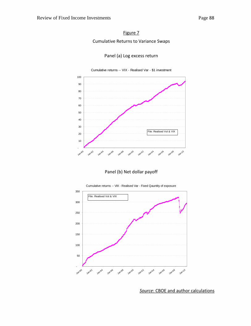
Review of Fixed Income Investments Page 88
Figure 7
Cumulative Returns to Variance Swaps
Panel (a) Log excess return
Cumulative returns -- VIX - Realised Var - $1 investment
-
10
20
30
40
50
60
70
80
90
100
Jan-90Jan-92
Jan-94Jan-96
Jan-98Jan-00
Jan-02Jan-04
Jan-06Jan-08
Jan-10
File: Realised Vol & VIX
Panel (b) Net dollar payoff
Cumulative returns -- VIX - Realised Var - Fixed Qauntity of exposure
-
50
100
150
200
250
300
350
Jan-90Jan-92
Jan-94Jan-96
Jan-98Jan-00
Jan-02Jan-04
Jan-06Jan-08
Jan-10
File: Realised Vol & VIX
Source: CBOE and author calculations

Review of Fixed Income Investments Page 89
Figure 8
Distribution of Returns to Variance Swaps and S&P
0.0%
5.0%
10.0%
15.0%
20.0%
25.0%
-16%
-13%
-10% -7% -4% -1% 2% 5% 8% 11
%14
%17
%
Scaled variance SwapS&P Monthly Return
Source: CBOE and author calculations

Review of Fixed Income Investments Page 90
Tables

Review of Fixed Income Investments Page 91
Table 1
Composition of the Barclays Global Aggregate Index (Feb. 2011)
# Issues % Nom Maturity Amt Out ($MM) Market Val ($MM)U.S. Agg: 300MM 5,285 38% 7.276 13,668,607 14,426,399Pan-Euro: 300MM 4,521 34% 7.888 12,286,940 12,762,912Asian-Pac Agg: 35B Yen 1,933 23% 7.464 8,253,408 8,544,250Eurodollar: 300MM 322 1% 3.874 274,928 284,787144A: 300MM 783 2% 7.776 714,954 759,313Canadian: 300MM 501 3% 9.737 924,466 1,001,082Euro-Yen: 35B Yen 31 0% 4.694 23,736 24,391Other Currencies 75 1% 9.290 198,267 197,821Global Aggregate 13,451 100% 7.582 36,345,306 38,000,951
Source: Barclays Capital.

Review of Fixed Income Investments Page 92
Table 2
Factors used in the Analysis
Variable DescriptionTreasury Returns
1 US_long US Treasury Long Bonds2 US_short US Treasury 1 - 5 year3 UK_long Sterling gilts 5-10 year4 UK_short Sterling gilts 1 -5 year5 Euro_long Euro Agggregate 10+ year6 Euro_short Euro Agggregate 1 - 3 year7 Asia_yc Asian-Pacific Non-Japan treasury8 Jap_yc Japan treasury
Fama-French & Liquidity9 SMB Small-minus-big10 HML High-minus-low11 Momn Momentum12 VIX VIX13 vol_swap Returns to Volatility Swap14 Refco REFCO - treasury yield spread15 Cr_spread US Corporate AAA - BBB spread
Stock Market16 S&P S&P 50017 ftse FTSE All Share18 eurostoxx Eurostoxx19 nikkei Nikkei 22520 snp_asia S&P Asia

Review of Fixed Income Investments Page 93
Table 3 Estimates of Risk Premia on US Treasury Bonds 1900 –2000

Review of Fixed Income Investments Page 94
Table 4
Estimates of Risk Premia on US Treasury Bonds: 1952 – 2010
Panel a: Jan 1952 to Dec 1981
Start 19520131 1-yr 2-yr 3-yr 4yr 5-yr 10-yr > 10 yrEnd 19811231Mean 0.04% 0.03% 0.02% 0.00% -0.03% -0.05% -0.22%Mean (ann) 0.43% 0.37% 0.26% 0.01% -0.37% -0.55% -2.61%Stdev 0.29% 0.71% 1.03% 1.23% 1.40% 1.64% 1.96%Max 2.26% 5.59% 8.08% 7.68% 8.80% 9.67% 12.86%Min -1.27% -3.92% -5.87% -6.69% -6.76% -8.33% -8.71%Count 360 360 360 360 360 360 360t-mean 2.34 0.84 0.39 0.01 -0.42 -0.53 -2.11
Panel b: Jan 1982 to Sep 2010
Start 19820129 1-yr 2-yr 3-yr 4yr 5-yr 10-yr > 10 yrEnd 20100930Mean 0.07% 0.15% 0.22% 0.27% 0.30% 0.35% 0.49%Mean (ann) 0.90% 1.86% 2.61% 3.26% 3.55% 4.25% 5.89%Stdev 0.19% 0.50% 0.82% 1.10% 1.34% 1.72% 2.83%Max 1.23% 2.10% 2.84% 3.59% 4.37% 6.64% 12.85%Min -1.01% -1.97% -2.99% -3.23% -3.73% -5.03% -8.59%Count 345 345 345 345 345 345 345t-mean 7.23 5.73 4 93 4.61 4.09 3.81 3.22
Panel c: Jan 1952 to Dec 1999
Start 19520131 1-yr 2-yr 3-yr 4yr 5-yr 10-yr > 10 yrEnd 19991231Mean 0.06% 0.09% 0.10% 0.11% 0.09% 0.11% 0.05%Mean (ann) 0.71% 1.06% 1.23% 1.29% 1.10% 1.34% 0.57%Stdev 0.26% 0.65% 0.97% 1.20% 1.39% 1.71% 2.31%Max 2.26% 5.59% 8.08% 7.68% 8.80% 9.67% 12.86%Min -1.27% -3.92% -5.87% -6.69% -6.76% -8.33% -8.71%Count 576 576 576 576 576 576 576t-mean 5.40 3.26 2 53 2.15 1.58 1.57 0.49
Panel d: Jan 2000 to Sep 2010
Start 20000131 1-yr 2-yr 3-yr 4yr 5-yr 10-yr > 10 yrEnd 20100930Mean 0.04% 0.11% 0.18% 0.25% 0.30% 0.32% 0.49%Mean (ann) 0.44% 1.29% 2.19% 2.99% 3.56% 3.82% 5.93%Stdev 0.17% 0.45% 0.76% 1.04% 1.33% 1.58% 2.98%Max 0.66% 1.44% 2.14% 2.82% 4.37% 6.64% 12.85%Min -1.01% -1.97% -2.99% -3.23% -3.73% -5.03% -8.59%Count 129 129 129 129 129 129 129t-mean 2.46 2.74 2.72 2.71 2.54 2.28 1.89
Panel e: Jan 1952 to Sep 2010
Start 19520131 1-yr 2-yr 3-yr 4yr 5-yr 10-yr > 10 yrEnd 20100930Mean 0.05% 0.09% 0.12% 0.13% 0.13% 0.15% 0.13%Mean (ann) 0.66% 1.10% 1.41% 1.60% 1.55% 1.79% 1.55%Stdev 0.25% 0.62% 0.94% 1.17% 1.38% 1.69% 2.45%Max 2.26% 5.59% 8.08% 7.68% 8.80% 9.67% 12.86%Min -1.27% -3.92% -5.87% -6.69% -6.76% -8.33% -8.71%Count 705 705 705 705 705 705 705t-mean 5.89 3.95 3 32 3.02 2.48 2.35 1.40
Source: Author calculation

Review of Fixed Income Investments Page 95
Table 5 Summary Statistics on the Fama-French Factors
Panel (a) 1973 - 2010
Rm-Rf SMB HML MomMean 0.43 0.27 0.36 0.72SD 4.69 3.06 3.54 4.64Max 16.01 14.62 19.72 18.35Min -23.00 -11.60 -20.79 -34.69Ann mean 5.15 3.19 4.30 8.59Ann SD 16.23 10.61 12.26 16.09N 449 449 449 449T-Mean 1.94 1.84 2.14 3.27
Correlation
Rm-Rf SMB HML MomRm-Rf 1 0.29 -0.21 -0.14SMB 1 -0.14 -0.11HML 1 -0.51Mom 1
Panel (b) 1927 - 2010
Rm-Rf SMB HML MomMean 0.61 0.26 0.35 0.70SD 5.43 3.24 3.73 4.83Max 37.43 37.63 35.95 18.35Min -28.37 -11.60 -20.79 -50.63Ann mean 7.37 3.09 4.15 8.37Ann SD 18.81 11.23 12.94 16.72N 1002 1002 1002 1002T-Mean 3.58 2.51 2.93 4.57
Correlation
Rm-Rf SMB HML MomRm-Rf 1 0.34 0.24 -0.34SMB 1 0.12 -0.20HML 1 -0.53Mom 1
Source: K. French website and author calculations

Review of Fixed Income Investments Page 96
Table 6
Summary Statistics on Monthly Excess Returns on Constant Dollar Exposure in
Variance Swap Exposure
Const $Variance
S&P Swap Mean 0.7% 5.5%Stdev 4.4% 4.4%Max 10.8% 17.6%Min -18.4% -6.1%Count 243 243 t=mean 2.39 19.50
Source: CBOE and author calculations
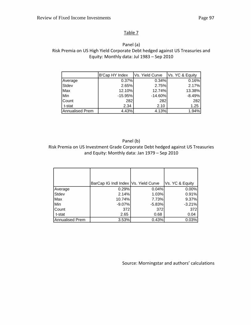
Review of Fixed Income Investments Page 97
Table 7
Panel (a) Risk Premia on US High Yield Corporate Debt hedged against US Treasuries and
Equity: Monthly data: Jul 1983 – Sep 2010
B'Cap HY Index Vs. Yield Curve Vs. YC & EquityAverage 0.37% 0.34% 0.16%Stdev 2.65% 2.75% 2.17%Max 12.10% 12.74% 13.38%Min -15.95% -14.60% -8.49%Count 282 282 282t-stat 2.34 2.10 1.25
Annualised Prem 4.43% 4.13% 1.94%
Panel (b) Risk Premia on US Investment Grade Corporate Debt hedged against US Treasuries
and Equity: Monthly data: Jan 1979 – Sep 2010
BarCap IG Indl Index Vs. Yield Curve Vs. YC & EquityAverage 0.29% 0.04% 0.00%Stdev 2.14% 1.03% 0.91%Max 10.74% 7.73% 9.37%Min -9.07% -5.83% -3.21%Count 372 372 372t-stat 2.65 0.68 0.04
Annualised Prem 3.53% 0.43% 0.03%
Source: Morningstar and authors’ calculations

Review of Fixed Income Investments Page 98
Table 8
Summary Statistics on Factor Returns
Start End Nobs mean stdev median min max t-meanUS_long 28-Feb-73 30-Sep-10 452 0.31 3.00 0.38 -9.02 13.56 2.19US_short 27-Feb-76 30-Sep-10 416 0.17 1.00 0.15 -5.07 7.11 3.41UK long 26-Feb-99 30-Sep-10 140 0.25 1.78 0.30 -4.66 6.05 1.68UK short 26-Feb-99 30-Sep-10 140 0.22 0.64 0.18 -1.32 2.33 4.10Eur long 31-Jul-98 30-Sep-10 147 0.32 2.04 0.41 -3.92 7.87 1.90Eur short 31-Jul-98 30-Sep-10 147 0.10 0.44 0.08 -0.84 1.54 2.77Asia yc 31-Aug-00 30-Sep-10 122 0.13 0.85 0.19 -1.86 3.69 1.71Japan yc 31-Aug-00 30-Sep-10 122 -0.03 0.63 0.00 -2.30 1.82 -0.53
SMB 28-Feb-73 30-Jun-10 449 0.24 3.23 0.09 -16.85 21.99 1.58HML 28-Feb-73 30-Jun-10 449 0.45 3.11 0.41 -12.37 13.87 3.04Momentum 28-Feb-73 30-Jun-10 449 0.72 4.64 0.81 -34.69 18.35 3.27VIX 28-Feb-90 30-Sep-10 248 1.17 18.25 -1.67 -32.97 90.67 1.01Vol_swap 31-Jan-90 31-Mar-10 243 0.04 0.04 0.04 -0.15 0.15 15.59Refco 31-May-91 30-Sep-10 236 0.00 0.08 0.00 -0.31 0.46 0.18Cr_spread 28-Feb-73 31-May-10 448 0.01 0.22 0.00 -1.18 1.95 0.49
S&P 28-Feb-73 30-Sep-10 452 0.28 4.62 0.59 -22.21 15.99 1.30FTSE 28-Feb-73 30-Sep-10 452 0.51 5.89 1.01 -27.59 51.94 1.83Eurostoxx 30-Jan-87 30-Sep-10 285 0.28 5.52 0.77 -22.83 15.57 0.87Nikkei 28-Feb-73 30-Sep-10 452 -0.15 5.66 -0.13 -24.57 19.58 -0.56S&P Asia 27-Feb-98 30-Sep-10 152 1.04 7.54 0.01 -19.18 29.95 1.70
Refco_ret_spread 31-May-91 30-Sep-10 236 0.01 0.80 0.01 -4.50 3.19 0.15
Source: BarCap, Morningstar and Author Calculations

Review of Fixed Income Investments Page 99
Table 9
Correlation Matrix of Factor Returns
Panel (a): Correlation between treasury returns
US_long US_short UK_long UK_short Eur_long Eur_short Asia_yc Japan_ycUS_long 1 0.77 0.82 0.59 0.75 0.46 0.55 0.35US_short 1 0.65 0.73 0.57 0.69 0.62 0.35UK_long 1 0.77 0.78 0 53 0.55 0.41UK_short 1 0.60 0.75 0.65 0.44Eur_long 1 0 56 0.55 0.31Eur_short 1 0.70 0.37Asia_yc 1 0.40Japan_yc 1SMBHMLMomentumVIXVol_swapRefcoCr_spreadS&PFTSEEurostoxxNikkeiS&P_Asia
Panel (b) : Correlation between F-F, liquidity and other returns
SMB HML Momentum VIX Vol_swap Refco Cr_spread S&P FTSE Eurostoxx Nikkei S&P_AsiaUS_long -0.13 0.12 0.14 0.12 -0.10 0.16 0 27 -0.09 -0.09 -0.23 -0.10 -0.17US_short -0.26 0.09 0.14 0.36 -0.36 0.17 0.49 -0.31 -0.37 -0.49 -0.38 -0.38UK_long -0.08 0.08 0.05 0.15 -0.11 0.15 0 31 -0.13 -0.12 -0.23 -0.13 -0.18UK_short -0.17 0.03 0.08 0.31 -0.30 0 29 0 33 -0.30 -0.28 -0.40 -0.36 -0.35Eur_long 0.01 0.12 -0.05 0.07 0.02 0 02 0.15 -0.12 -0.07 -0.15 -0.08 -0.08Eur_short -0.07 0.01 0.01 0.33 -0.32 0.14 0 30 -0.36 -0.38 -0.47 -0.43 -0.34Asia_yc 0.00 0.14 -0.08 0.12 -0.20 0 33 0 25 -0.12 -0.15 -0.26 -0.24 -0.22Japan_yc 0.06 -0.03 -0.05 0.00 -0.06 0 27 0.13 -0.07 -0.07 -0.11 -0.28 -0.14SMB 1 -0.07 -0.23 -0.30 0.30 0 02 -0 20 0.28 0.29 0.35 0.29 0.38HML 1 0.10 0.16 0.04 0.10 0 04 -0.07 -0.01 -0.04 -0.01 -0.11Momentum 1 0.25 -0.10 0.11 0.19 -0.52 -0.45 -0.52 -0.29 -0.49VIX 1 -0.65 0 26 0 21 -0.62 -0.68 -0.66 -0.51 -0.60Vol_swap 1 -0 25 -0 26 0.48 0.54 0.54 0.47 0.46Refco 1 0 05 -0.12 -0.08 -0.14 -0.23 -0.20Cr_spread 1 -0.156 -0.183 -0.27 -0.21 -0.21S&P 1 0.88 0.88 0.63 0.79FTSE 1 0.92 0.64 0.75Eurostoxx 1 0.67 0.79Nikkei 1 0.66S&P_Asia 1
Note on formatting: Yellow: correlation >0.3. Blue: Correlation < -0.3.
Source: BarCap, Morningstar and author calculations

Review of Fixed Income Investments Page 100
Table 10 Summary Statistics on BGAI and its Components
Start End Nobs mean stdev median min max T-Mean1 Global_agg hedged 28-Feb-90 30-Sep-10 248 0.28 0.88 0.33 -2.15 3.02 5.022 US_treas GL_elig hedged 31-Oct-00 30-Sep-10 120 0.33 1.47 0.44 -4.47 5.31 2.463 US_govt GL_elig hedged 28-Feb-01 30-Sep-10 116 0 32 1.15 0.38 -3.81 3.76 3.044 US_corp GA_elig hedged 31-Oct-00 30-Sep-10 120 0.40 1.86 0.48 -8.07 6.89 2.355 US_secur GA_elig hedged 31-Oct-00 30-Sep-10 120 0 33 0.85 0.35 -2.12 2.80 4.22
6 US_agg GA_elig 30-Nov-00 30-Sep-10 119 0 34 1.12 0.47 -3.42 3.75 3.337 Pan_Euro GA_elig hedged 30-Nov-00 30-Sep-10 119 0 26 0.95 0.31 -1.82 2.94 3.018 Asia_Pac GA_elig hedged 30-Nov-00 30-Sep-10 119 0 21 0.57 0.21 -1.98 2.08 4.039 Canadian GA_elig hedged 30-Nov-00 30-Sep-10 119 0 35 1.10 0.42 -2.28 3.25 3.4510 Other GA_elig hedged 28-Feb-05 30-Sep-10 68 0 23 1.93 0.43 -5.90 5.77 0.98
11 Euro_dol GA_eligible 30-Nov-00 30-Sep-10 119 0 32 0.91 0 37 -2.46 2.27 3.8612 144A GA_eligible 30-Nov-00 30-Sep-10 119 0 37 2.03 0 69 -12.49 4.41 2.0113 Euroyen GA_elig hedged 30-Nov-00 30-Sep-10 119 0.13 0.53 0.18 -1.69 1.38 2.7414 Apac_tre GA_elig hedged 31-Oct-00 30-Sep-10 120 0 22 0.60 0 23 -2.15 2.26 3.9515 Apac_gov GA_elig hedged 28-Feb-01 30-Sep-10 116 0.19 0.51 0 21 -1.59 1.47 3.92
16 Apac_corp GA_elig hedged 31-Oct-00 30-Sep-10 120 0.19 0.41 0 21 -1.30 1.15 5.0717 Apac_sec GA_elig hedged 31-Oct-00 30-Sep-10 120 0.16 0.51 0.13 -1.33 1 87 3.4218 Euro_tre GA_elig hedged 31-Oct-00 30-Sep-10 120 0 27 1.04 0 35 -1.71 3.73 2.8519 Euro_gov GA_elig hedged 28-Feb-01 30-Sep-10 116 0 26 0.90 0 29 -1.65 2 62 3.0920 Euro_corp GA_elig hedged 31-Oct-00 30-Sep-10 120 0 26 1.14 0 36 -5.15 3.47 2.45
21 Euro_sec GA_elig hedged 31-Oct-00 30-Sep-10 120 0 25 0.82 0 26 -1.39 2 29 3.3522 US_securitised 28-Feb-97 30-Sep-10 164 0 27 0.80 0 29 -2.21 2.74 4.3323 US_government 28-Feb-94 30-Sep-10 200 0 24 1.15 0 27 -3.78 3.78 3.0024 US_corporate 28-Feb-90 30-Sep-10 248 0 34 1.61 0.44 -7.85 6.79 3.3725 US_corp_inter 28-Feb-90 30-Sep-10 248 0 31 1.30 0 38 -7.22 4.49 3.78
26 US_corporate_long 28-Feb-90 30-Sep-10 248 0.43 2.53 0 54 -11.24 14.12 2.6627 US_high_yield 28-Feb-90 30-Sep-10 248 0.47 2.76 0 64 -15.93 12.10 2.7028 US_aggregate 27-Feb-76 30-Sep-10 416 0 25 1.66 0 34 -7.06 10.57 3.0229 US_treasuries 31-Jan-73 30-Sep-10 453 0 22 1.57 0 25 -6.04 8.75 2.9330 UK_agg hedged 31-Mar-99 30-Sep-10 139 0 09 1.50 0.14 -6.76 4 35 0.7331 UK_treasuries hedged 26-Feb-99 30-Sep-10 140 0.13 1.49 0.15 -4.84 5 04 1.0532 GPFG_BM hedged 1-Jan-98 30-Sep-10 153 0.18 0.97 0 20 -2.29 3.47 2.3033 Actual_ret hedged 30-Jan-98 30-Sep-10 153 0 22 1.06 0.27 -3.39 3.08 2.5234 Active_ret hedged 30-Jan-98 30-Sep-10 153 0.02 0.36 0.02 -1.79 1.51 0.62
Comparison Start End Nobs mean stdev median min max T-MeanGlobal_agg hedged 1-Jan-98 30-Sep-10 153 0.25 0.81 0.31 -2.14 2.71 3.82GPFG_BM hedged 1-Jan-98 30-Sep-10 153 0.18 0.97 0.20 -2.29 3.47 2.30
Source: BarCap, Morningstar and author calculations

Table 11 Regression of BGAI on Factors
Panel (a) 1999-2010
Start Feb-99 Feb-99 Feb-99 Feb-99 Feb-99 Feb-99 Feb-99 Feb-99 Feb-99 Feb-99 Feb-99 Feb-99 Feb-99 Feb-99End Sep-10 Sep-10 Jun-10 Sep-10 Sep-10 Mar-10 Mar-10 Mar-10 Mar-10 May-10 May-10 Mar-10 Mar-10 Mar-10Constant 0.08 0.07 0.06 0.08 0.07 -0.04 -0.02 0.00 0.00 0.07 0.06 -0.03 -0.02 0.00
3.00 2.65 2.30 3.06 2.81 -1.06 -0.53 0.11 0.09 2.71 2.44 -1.05 -0.48 0.10US_long 0.11 0.11 0.11 0.10 0.11 0.11 0.10 0.10 0.10 0.10 0.10 0.10 0.10 0.10
5.34 5.84 5.82 5.67 5.87 5.54 5.63 5.47 5.55 5.18 5.37 5.32 5.46 5.29US_short 0.25 0.28 0.28 0.31 0.31 0.29 0.30 0.31 0.32 0.38 0.38 0.35 0.37 0.39
3.34 4.05 3.87 4.55 4.59 3.96 4.38 4.47 4.59 5.02 5.16 4.61 5.14 5.35UK_long 0.00 -0.01 -0.01 0.01 0.00 0.00 -0.01 0.00 -0.01 0.02 0.01 0.01 0.00 0.01
0.07 -0.39 -0.29 0.17 -0.15 -0.01 -0.37 0.06 -0.24 0.64 0.28 0.38 0.02 0.19UK_short 0.00 0.05 0.06 0.02 0.05 0.04 0.06 0.03 0.05 0.03 0.06 0.06 0.09 0.07
-0.05 0.65 0.74 0.27 0.60 0.48 0.79 0.40 0.66 0.39 0.78 0.74 1.12 0.91Eur_long 0.14 0.14 0.13 0.13 0.13 0.13 0.14 0.13 0.13 0.12 0.12 0.12 0.12 0.12
6.22 6.59 5.94 6.20 6.42 6.04 6.43 6.20 6.42 5.69 5.93 5.45 5.84 5.87Eur_short 0.24 0.29 0.27 0.28 0.30 0.30 0.33 0.33 0.34 0.29 0.30 0.28 0.31 0.32
2.43 3.22 2.87 3.18 3.43 3.25 3.67 3.63 3.81 3.28 3.58 3.12 3.59 3.72SMB 0.01
1.20HML 0.01
0.91Momentum -0.01
-1.51VIX -0.01 -0.01 -0.01 0.00 -0.01 0.00 0.00
-5.63 -3.14 -3.23 -1.85 -5.08 -2.67 -1.71Vol_swap 3.02 2.23 1.82 1.68 2.74 1.89 1.42
5.03 3.63 2.64 2.47 4.65 3.18 2.16Refco -0.48 -0.53 -0.53 -0.57 -0.50
-1.90 -2.15 -2.00 -2.26 -1.99Cr_spread -0.26 -0.26 -0.23 -0.24 -0.25
-3.26 -3.34 -2.79 -3.07 -3.14S&P 0.03 0.02 0.02 0.02 0.01 0.02 0.02 0.02
5.38 3.75 2.73 3.62 2.44 3.05 3.95 2.76R-squared 0.88 0.90 0.90 0.90 0.91 0.90 0.91 0.91 0.91 0.91 0.92 0.91 0.92 0.92N 140 140 137 140 140 134 134 134 134 136 136 134 134 134

Review of Fixed Income Investments Page 102
Panel (b) 1999-2004
Start Feb-99 Feb-99 Feb-99 Feb-99 Feb-99 Feb-99 Feb-99 Feb-99 Feb-99 Feb-99 Feb-99 Feb-99 Feb-99 Feb-99End Jan-04 Jan-04 Jan-04 Jan-04 Jan-04 Jan-04 Jan-04 Jan-04 Jan-04 Jan-04 Jan-04 Jan-04 Jan-04 Jan-04Constant 0.06 0.06 0.03 0.06 0.06 0.05 0.06 0.06 0.06 0.04 0.04 0.05 0.05 0.05
2.09 1.93 0.97 1.88 1.84 1.17 1.32 1.47 1.45 1.48 1.44 1.22 1.30 1.24US_long 0.11 0.11 0.11 0.11 0.11 0.11 0.11 0.11 0.11 0.09 0.08 0.08 0.09 0.09
4.96 4.98 4.58 5.05 5.00 4.73 4.82 4.93 4.89 3.63 3.57 3.67 3.72 3.53US_short 0.33 0.34 0.39 0.35 0.35 0.34 0.34 0.34 0.34 0.52 0.52 0.53 0.51 0.52
3.62 3.78 4.16 3.86 3.84 3.59 3.66 3.69 3.67 4.51 4.50 4.74 4.54 4.38UK_long 0.01 0.01 0.01 0.01 0.01 0.01 0.01 0.02 0.01 0.02 0.01 0.02 0.02 0.02
0.30 0.13 0.15 0.33 0.23 0.21 0.12 0.37 0.28 0.43 0.31 0.46 0.40 0.37UK_short 0.00 0.04 0.08 0.02 0.03 0.01 0.04 0.01 0.02 0.01 0.02 0.00 0.01 0.02
0.01 0.32 0.74 0.18 0.28 0.11 0.32 0.12 0.21 0.10 0.22 0.02 0.13 0.14Eur_long 0.10 0.10 0.08 0.10 0.10 0.10 0.10 0.10 0.09 0.10 0.10 0.10 0.10 0.10
3.04 2.93 2.34 3.00 2.93 3.04 2.86 2.88 2.81 3.29 3.23 3.26 3.12 3.08Eur_short 0.37 0.39 0.35 0.39 0.40 0.36 0.39 0.40 0.40 0.30 0.30 0.30 0.32 0.31
3.28 3.45 3.00 3.49 3.49 3.08 3.30 3.39 3.39 2.58 2.59 2.59 2.70 2.57SMB 0.01
1.40HML 0.01
1.51Momentum -0.01
-1.10VIX 0.00 0.00 0.00 0.00 0.00 0.00 0.00
-1.76 -0.99 -1.71 -1.01 -0.27 0.21 0.13Vol_swap 0.31 0.02 -0.19 -0.20 -0.17 -0.29 -0.26
0.40 0.03 -0.23 -0.25 -0.22 -0.37 -0.33Refco 0.08 0.12 0.07 0.10 0.11
0.16 0.25 0.15 0.22 0.23Cr_spread -0.49 -0.49 -0.53 -0.48 -0.49
-2.24 -2.23 -2.74 -2.40 -2.23S&P 0.01 0.01 0.00 0.01 0.00 0.01 0.01 0.01
1.55 1.58 0.58 1.48 0.59 0.73 0.81 0.74R-squared 0.94 0.95 0.95 0.95 0.95 0.94 0.95 0.95 0.95 0.95 0.95 0.95 0.95 0.95N 60 60 60 60 60 60 60 60 60 60 60 60 60 60

Review of Fixed Income Investments Page 103
Panel (c) 2004-2009
Start Feb-04 Feb-04 Feb-04 Feb-04 Feb-04 Feb-04 Feb-04 Feb-04 Feb-04 Feb-04 Feb-04 Feb-04 Feb-04 Feb-04End Jan-09 Jan-09 Jan-09 Jan-09 Jan-09 Jan-09 Jan-09 Jan-09 Jan-09 Jan-09 Jan-09 Jan-09 Jan-09 Jan-09Constant 0.03 0.04 0.06 0.05 0.04 -0.11 -0.04 -0.07 -0.02 0.04 0.04 -0.10 0.01 -0.01
0.61 1.03 1.94 1.22 1.25 -2.41 -0.78 -1.15 -0.31 1.11 1.25 -2.14 0.33 -0.12US_long 0.12 0.11 0.09 0.10 0.10 0.12 0.11 0.12 0.11 0.11 0.14 0.14 0.14 0.15
3.29 3.52 3.26 3.12 3.38 4.00 3.83 3.66 3.61 3.20 4.98 4.33 5.07 5.10US_short 0.11 0.27 0.30 0.23 0.29 0.18 0.26 0.21 0.27 0.20 0.14 0.13 0.16 0.13
0.91 2.82 3.47 2.20 3.07 1.88 2.80 2.13 2.86 1.62 1.40 1.22 1.78 1.30UK_long 0.10 0.01 0.05 0.10 0.03 0.10 0.04 0.10 0.04 0.11 0.01 0.11 0.03 0.02
1.33 0.14 0.77 1.54 0.47 1.53 0.57 1.56 0.62 1.77 0.19 1.80 0.47 0.32UK_short -0.15 -0.08 -0.15 -0.15 -0.10 -0.12 -0.08 -0.13 -0.09 -0.08 0.02 -0.05 0.01 0.02
-0.87 -0.58 -1.16 -1.06 -0.74 -0.84 -0.65 -0.92 -0.70 -0.58 0.20 -0.35 0.06 0.21Eur_long 0.11 0.16 0.16 0.10 0.14 0.07 0.12 0.08 0.12 0.08 0.11 0.05 0.10 0.10
2.92 5.07 5.71 2.95 4.45 2.25 3.65 2.39 3.63 2.20 4.05 1.48 3.46 3.40Eur_short 0.31 0.42 0.38 0.39 0.43 0.49 0.48 0.47 0.47 0.41 0.54 0.52 0.54 0.57
1.72 2.94 2.60 2.46 3.07 3.22 3.41 3.10 3.32 2.62 4.31 3.51 4.35 4.45SMB -0.01
-0.41HML -0.05
-3.74Momentum -0.01
-1.27VIX -0.01 0.00 0.00 0.00 -0.01 0.00 0.00
-4.39 -1.80 -1.25 -0.69 -3.51 0.52 0.99Vol_swap 4.48 2.32 3.31 1.80 3.93 0.77 1.29
5.12 2.19 2.59 1.39 4.58 0.76 1.14Refco -0.83 -1.43 -0.93 -1.27 -1.39
-2.17 -4.42 -2.72 -4.23 -4.30Cr_spread -0.04 0.19 0.01 0.15 0.18
-0.35 1.81 0.12 1.50 1.75S&P 0.05 0.05 0.04 0.04 0.04 0.06 0.05 0.06
5.80 5.37 3.76 3.17 2.93 5.50 4.59 4.63R-squared 0.88 0.93 0.95 0.92 0.93 0.92 0.94 0.93 0.94 0.92 0.95 0.93 0.95 0.95N 60 60 60 60 60 60 60 60 60 60 60 60 60 60

Review of Fixed Income Investments Page 104
Table 12 Regression of US Government Related Index on Factors 2001-2010
Start Feb-01 Feb-01 Feb-01 Feb-01 Feb-01 Feb-01 Feb-01 Feb-01 Feb-01 Feb-01 Feb-01 Feb-01 Feb-01 Feb-01 Feb-01End Sep-10 Sep-10 Sep-10 Jun-10 Sep-10 Sep-10 Mar-10 Mar-10 Mar-10 Mar-10 May-10 May-10 Mar-10 Mar-10 Mar-10Constant 0.08 0.07 0.04 0.04 0.06 0.04 -0.07 -0.04 -0.03 -0.03 0.04 0.02 -0.07 -0.04 -0.03
2.25 1.72 1.09 0.97 1.56 1.16 -1.37 -0.90 -0.52 -0.54 1.12 0.69 -1.60 -1.07 -0.70US_long 0.22 0.26 0.25 0.26 0.25 0.25 0.27 0.26 0.26 0.26 0.24 0.24 0.26 0.24 0.24
12.16 8.48 9.27 9.16 8.93 9.31 9.63 9.70 9.46 9.57 9.35 9.73 9.83 10.05 9.81US_short 0.64 0.52 0.58 0.52 0.63 0.63 0.54 0.57 0.57 0.59 0.74 0.75 0.68 0.74 0.75
8.20 4.81 6.14 5.08 6.35 6.64 5.25 5.84 5.62 5.91 7.29 7.86 6.82 7.85 7.86UK_long -0.10 -0.11 -0.11 -0.09 -0.10 -0.09 -0.10 -0.08 -0.09 -0.05 -0.06 -0.05 -0.06 -0.05
-1.87 -2.37 -2.25 -1.93 -2.26 -1.81 -2.12 -1.82 -2.07 -1.09 -1.39 -1.15 -1.43 -1.35UK_short 0.09 0.15 0.15 0.12 0.15 0.15 0.16 0.15 0.16 0.16 0.18 0.18 0.19 0.18
0.74 1.35 1.39 1.12 1.41 1.35 1.57 1.35 1.54 1.55 1.84 1.74 2.01 1.92Eur_long 0.02 0.02 0.02 0.01 0.01 -0.01 0.00 -0.01 0.00 -0.03 -0.02 -0.04 -0.03 -0.03
0.77 0.77 0.83 0.25 0.46 -0.34 0.01 -0.25 0.01 -0.96 -0.78 -1.47 -1.16 -1.14Eur_short 0.16 0.23 0.26 0.19 0.23 0.23 0.26 0.23 0.25 0.17 0.21 0.19 0.22 0.22
1.10 1.86 1.96 1.48 1.88 1.75 2.03 1.77 2.00 1.51 1.98 1.63 2.01 1.99SMB -0.01
-0.39HML 0.01
0.97Momentum 0.00
0.17VIX -0.01 -0.01 0.00 0.00 -0.01 0.00 0.00
-5.07 -2.50 -2.07 -0.90 -4.42 -2.07 -0.88Vol_swap 3.54 2.43 2.32 2.01 3.02 1.83 1.48
4.09 2.73 2.24 1.98 3.91 2.37 1.70Refco -0.95 -0.97 -1.00 -0.98 -0.94
-3.03 -3.30 -3.09 -3.30 -3.08Cr_spread -0.51 -0.51 -0.46 -0.49 -0.50
-5.21 -5.56 -4.69 -5.32 -5.37S&P 0.04 0.04 0.03 0.02 0.02 0.03 0.03 0.02
5.67 4.12 3.42 3.32 2.69 3.73 4.18 3.49R-squared 0.89 0.89 0.92 0.92 0.91 0.92 0.92 0.93 0.92 0.93 0.94 0.95 0.94 0.95 0.95N 116 116 116 113 116 116 110 110 110 110 112 112 110 110 110

Table 13 Regression of US Investment Grade Corporate Debt on Factors 2000-2010
Panel (a) 2000 - 2010: Start Oct-00 Oct-00 Oct-00 Oct-00 Oct-00 Oct-00 Oct-00 Oct-00 Oct-00 Oct-00 Oct-00 Oct-00 Oct-00 Oct-00 Oct-00End Sep-10 Sep-10 Sep-10 Jun-10 Sep-10 Sep-10 Mar-10 Mar-10 Mar-10 Mar-10 May-10 May-10 Mar-10 Mar-10 Mar-10Constant 0.26 0.26 0.14 0.15 0.20 0.15 -0.43 -0.32 -0.16 -0.16 0.11 0.07 -0.43 -0.32 -0.18
1.81 1.69 1.07 1.07 1.52 1.20 -2.25 -1.77 -0.81 -0.85 0.93 0.57 -2.40 -1.91 -1.03US_long 0.43 0.46 0.43 0.49 0.42 0.41 0.44 0.41 0.41 0.39 0.41 0.40 0.45 0.41 0.39
6.00 3.90 4.16 4.55 4.17 4.26 4.10 4.01 4.01 3.96 4.09 4.13 4.26 4.20 4.03US_short -0.40 -0.33 -0.11 -0.25 0.12 0.11 -0.07 0.06 0.13 0.16 0.38 0.41 0.21 0.37 0.50
-1.35 -0.81 -0.29 -0.65 0.34 0.33 -0.17 0.16 0.36 0.45 0.99 1.10 0.52 1.00 1.37UK_long -0.36 -0.40 -0.42 -0.33 -0.36 -0.34 -0.38 -0.33 -0.36 -0.24 -0.27 -0.28 -0.32 -0.29
-1.76 -2.20 -2.32 -1.88 -2.10 -1.81 -2.15 -1.88 -2.09 -1.42 -1.68 -1.58 -1.92 -1.77UK_short 0.01 0.24 0.27 0.20 0.27 0.15 0.23 0.17 0.22 0.36 0.42 0.43 0.51 0.44
0.03 0.56 0.64 0.50 0.69 0.35 0.57 0.42 0.56 0.89 1.09 1.01 1.29 1.15Eur_long 0.27 0.25 0.23 0.18 0.20 0.15 0.19 0.16 0.19 0.09 0.11 0.04 0.08 0.09
2.16 2.30 1.94 1.68 1.88 1.21 1.66 1.42 1.68 0.86 1.09 0.36 0.79 0.83Eur_short -0.07 0.24 0.16 0.09 0.22 0.44 0.56 0.44 0.53 0.14 0.29 0.29 0.42 0.40
-0.13 0.50 0.32 0.20 0.48 0.83 1.14 0.90 1.10 0.32 0.67 0.60 0.94 0.91SMB 0.00
0.04HML 0.00
-0.08Momentum -0.05
-2.13VIX -0.04 -0.03 -0.03 -0.02 -0.04 -0.03 -0.02
-6.58 -3.97 -4.01 -2.66 -5.87 -3.42 -2.53Vol_swap 16.97 12.12 8.51 7.60 14.84 9.75 5.95
5.03 3.55 2.24 2.04 4.68 3.10 1.75Refco -3.79 -3.92 -4.46 -4.50 -4.00
-3.07 -3.31 -3.34 -3.65 -3.28Cr_spread -1.36 -1.36 -1.21 -1.28 -1.33
-3.51 -3.66 -2.94 -3.39 -3.60S&P 0.15 0.10 0.08 0.11 0.07 0.09 0.11 0.08
5.77 3.26 2.75 3.86 2.44 3.17 4.42 2.99R-squared 0.34 0.38 0.52 0.54 0.56 0.58 0.52 0.58 0.58 0.60 0.63 0.66 0.59 0.66 0.68N 120 120 120 117 120 120 114 114 114 114 116 116 114 114 114

Review of Fixed Income Investments Page 106
Panel (b): 2000 – 2005
Oct-00 Oct-00 Oct-00 Oct-00 Oct-00 Oct-00 Oct-00 Oct-00 Oct-00 Oct-00 Oct-00 Oct-00 Oct-00 Oct-00 Oct-00End Sep-05 Sep-05 Sep-05 Sep-05 Sep-05 Sep-05 Sep-05 Sep-05 Sep-05 Sep-05 Sep-05 Sep-05 Sep-05 Sep-05 Sep-05Constant 0.18 0.23 0.17 -0.05 0.15 0.14 -0.06 -0.01 0.09 0.07 0.00 0.00 -0.11 -0.14 -0.08
1.71 1.62 1.32 -0.32 1.20 1.15 -0.29 -0.03 0.53 0.44 0.00 0.02 -0.83 -1.08 -0.63US_long 0.45 0.43 0.38 0.38 0.40 0.39 0.38 0.36 0.40 0.38 0.26 0.26 0.23 0.23 0.24
6.83 4.41 4.55 4.68 4.99 4.89 4.03 4.26 4.76 4.65 3.95 3.86 3.54 3.35 3.59US_short 0.05 0.23 0.49 0.48 0.54 0.59 0.53 0.65 0.59 0.64 1.34 1.34 1.45 1.51 1.42
0.18 0.63 1.52 1.62 1.76 1.93 1.40 1.93 1.80 1.99 4.93 5.00 5.28 5.30 5.04UK_long 0.11 0.09 -0.16 0.18 0.15 0.04 0.05 0.17 0.13 0.02 0.02 -0.02 -0.05 -0.01
0.43 0.42 -0.72 0.86 0.73 0.18 0.24 0.76 0.62 0.13 0.12 -0.15 -0.31 -0.04UK_short -0.51 -0.37 0.20 -0.35 -0.32 -0.34 -0.27 -0.32 -0.29 0.04 0.02 0.08 0.12 0.07
-1.04 -0.86 0.47 -0.85 -0.80 -0.71 -0.64 -0.77 -0.71 0.13 0.07 0.24 0.37 0.21Eur_long 0.02 0.01 0.04 -0.02 -0.01 0.02 0.01 -0.02 -0.01 0.01 0.01 0.02 0.03 0.01
0.15 0.10 0.32 -0.16 -0.10 0.14 0.09 -0.15 -0.09 0.10 0.10 0.18 0.25 0.13Eur_short 0.05 0.23 0.24 0.04 0.13 -0.08 0.13 0.01 0.10 -0.12 -0.04 -0.08 -0.21 -0.08
0.09 0.46 0.53 0.09 0.29 -0.15 0.26 0.03 0.22 -0.34 -0.11 -0.21 -0.55 -0.22SMB 0.04
1.36HML 0.09
2.57Momentum -0.06
-3.13VIX -0.03 -0.02 -0.03 -0.02 -0.01 -0.01 -0.01
-4.85 -2.76 -4.15 -2.36 -2.19 -1.09 -0.69Vol_swap 7.24 4.45 1.48 1.70 2.88 3.79 2.28
2.16 1.44 0.46 0.54 1.26 1.63 0.93Refco -2.83 -2.26 -2.19 -3.01 -2.27
-2.01 -1.56 -1.52 -2.10 -1.56Cr_spread -3.50 -3.38 -3.54 -3.99 -3.40
-6.15 -5.94 -6.64 -7.91 -5.96S&P 0.10 0.09 0.05 0.09 0.05 0.03 0.04 0.03
4.23 2.82 1.81 3.81 1.82 1.43 2.13 1.46R-squared 0.73 0.74 0.81 0.85 0.82 0.83 0.76 0.81 0.82 0.83 0.90 0.90 0.90 0.89 0.90N 60 60 60 60 60 60 60 60 60 60 60 60 60 60 60
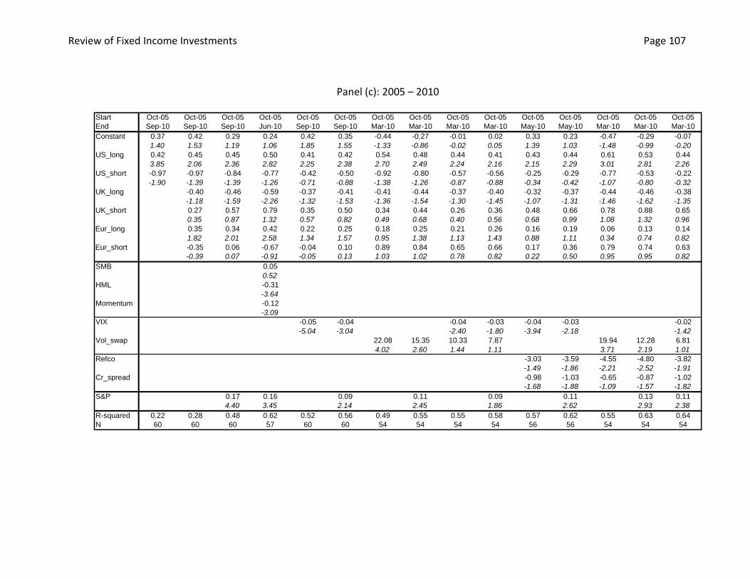
Review of Fixed Income Investments Page 107
Panel (c): 2005 – 2010
Start Oct-05 Oct-05 Oct-05 Oct-05 Oct-05 Oct-05 Oct-05 Oct-05 Oct-05 Oct-05 Oct-05 Oct-05 Oct-05 Oct-05 Oct-05End Sep-10 Sep-10 Sep-10 Jun-10 Sep-10 Sep-10 Mar-10 Mar-10 Mar-10 Mar-10 May-10 May-10 Mar-10 Mar-10 Mar-10Constant 0.37 0.42 0.29 0.24 0.42 0.35 -0.44 -0.27 -0.01 0.02 0.33 0.23 -0.47 -0.29 -0.07
1.40 1.53 1.19 1.06 1.85 1.55 -1.33 -0.86 -0.02 0.05 1.39 1.03 -1.48 -0.99 -0.20US_long 0.42 0.45 0.45 0.50 0.41 0.42 0.54 0.48 0.44 0.41 0.43 0.44 0.61 0.53 0.44
3.85 2.06 2.36 2.82 2.25 2.38 2.70 2.49 2.24 2.16 2.15 2.29 3.01 2.81 2.26US_short -0.97 -0.97 -0.84 -0.77 -0.42 -0.50 -0.92 -0.80 -0.57 -0.56 -0.25 -0.29 -0.77 -0.53 -0.22
-1.90 -1.39 -1.39 -1.26 -0.71 -0.88 -1.38 -1.26 -0.87 -0.88 -0.34 -0.42 -1.07 -0.80 -0.32UK_long -0.40 -0.46 -0.59 -0.37 -0.41 -0.41 -0.44 -0.37 -0.40 -0.32 -0.37 -0.44 -0.46 -0.38
-1.18 -1.59 -2.26 -1.32 -1.53 -1.36 -1.54 -1.30 -1.45 -1.07 -1.31 -1.46 -1.62 -1.35UK_short 0.27 0.57 0.79 0.35 0.50 0.34 0.44 0.26 0.36 0.48 0.66 0.78 0.88 0.65
0.35 0.87 1.32 0.57 0.82 0.49 0.68 0.40 0.56 0.68 0.99 1.08 1.32 0.96Eur_long 0.35 0.34 0.42 0.22 0.25 0.18 0.25 0.21 0.26 0.16 0.19 0.06 0.13 0.14
1.82 2.01 2.58 1.34 1.57 0.95 1.38 1.13 1.43 0.88 1.11 0.34 0.74 0.82Eur_short -0.35 0.06 -0.67 -0.04 0.10 0.89 0.84 0.65 0.66 0.17 0.36 0.79 0.74 0.63
-0.39 0.07 -0.91 -0.05 0.13 1.03 1.02 0.78 0.82 0.22 0.50 0.95 0.95 0.82SMB 0.05
0.52HML -0.31
-3.64Momentum -0.12
-3.09VIX -0.05 -0.04 -0.04 -0.03 -0.04 -0.03 -0.02
-5.04 -3.04 -2.40 -1.80 -3.94 -2.18 -1.42Vol_swap 22.08 15.35 10.33 7.87 19.94 12.28 6.81
4.02 2.60 1.44 1.11 3.71 2.19 1.01Refco -3.03 -3.59 -4.55 -4.80 -3.82
-1.49 -1.86 -2.21 -2.52 -1.91Cr_spread -0.98 -1.03 -0.65 -0.87 -1.02
-1.68 -1.88 -1.09 -1.57 -1.82S&P 0.17 0.16 0.09 0.11 0.09 0.11 0.13 0.11
4.40 3.45 2.14 2.45 1.86 2.62 2.93 2.38R-squared 0.22 0.28 0.48 0.62 0.52 0.56 0.49 0.55 0.55 0.58 0.57 0.62 0.55 0.63 0.64N 60 60 60 57 60 60 54 54 54 54 56 56 54 54 54

Review of Fixed Income Investments Page 108
Table 14 Regression of US Securitised Debt (MBS, ABS, CMBS) on Factors
Start Oct-00 Oct-00 Oct-00 Oct-00 Oct-00 Oct-00 Oct-00 Oct-00 Oct-00 Oct-00 Oct-00 Oct-00 Oct-00 Oct-00 Oct-00End Sep-10 Sep-10 Sep-10 Jun-10 Sep-10 Sep-10 Mar-10 Mar-10 Mar-10 Mar-10 May-10 May-10 Mar-10 Mar-10 Mar-10Constant 0.16 0.17 0.14 0.16 0.15 0.14 0.08 0.11 0.14 0.13 0.13 0.11 0.08 0.12 0.13
3.42 3.36 2.96 3.43 3.27 2.98 1.12 1.78 1.94 1.99 3.24 2.93 1.32 2.22 2.28US_long 0.14 0.13 0.12 0.14 0.12 0.12 0.13 0.12 0.12 0.12 0.12 0.12 0.13 0.12 0.12
6.32 3.47 3.56 3.86 3.43 3.52 3.44 3.31 3.29 3.25 3.62 3.69 3.82 3.77 3.68US_short 0.44 0.48 0.54 0.47 0.56 0.56 0.50 0.55 0.55 0.56 0.68 0.69 0.65 0.70 0.71
4.63 3.60 4.38 3.69 4.37 4.52 3.63 4.20 4.01 4.28 5.24 5.68 4.91 5.92 5.92UK_long -0.01 -0.02 -0.01 0.00 -0.01 0.00 -0.01 0.00 -0.01 0.05 0.03 0.03 0.02 0.02
-0.11 -0.29 -0.19 -0.03 -0.23 -0.01 -0.24 0.02 -0.20 0.79 0.60 0.48 0.30 0.34UK_short -0.13 -0.07 -0.06 -0.09 -0.06 -0.09 -0.06 -0.08 -0.06 0.00 0.02 0.03 0.06 0.06
-0.83 -0.47 -0.45 -0.62 -0.44 -0.57 -0.40 -0.55 -0.41 -0.03 0.18 0.24 0.50 0.45Eur_long 0.04 0.03 0.04 0.02 0.03 0.03 0.05 0.04 0.05 -0.02 -0.01 -0.02 0.00 0.00
0.94 0.91 0.96 0.55 0.75 0.74 1.18 0.84 1.17 -0.43 -0.22 -0.47 -0.07 -0.06Eur_short 0.08 0.17 0.14 0.11 0.17 0.10 0.15 0.10 0.14 0.07 0.13 0.03 0.08 0.08
0.46 1.01 0.84 0.67 1.00 0.54 0.84 0.56 0.81 0.44 0.89 0.21 0.56 0.55SMB -0.02
-1.46HML 0.01
0.49Momentum -0.01
-1.74VIX -0.01 0.00 -0.01 0.00 -0.01 0.00 0.00
-3.47 -1.16 -2.44 -0.94 -2.68 -0.27 -0.57Vol_swap 2.48 0.74 0.59 0.16 1.50 -0.35 -0.63
2.09 0.62 0.42 0.12 1.45 -0.35 -0.56Refco -1.67 -1.72 -2.02 -2.03 -1.99
-4.02 -4.41 -4.63 -5.18 -5.00Cr_spread -0.59 -0.59 -0.59 -0.62 -0.62
-4.56 -4.86 -4.43 -5.14 -5.15S&P 0.04 0.03 0.03 0.04 0.03 0.03 0.04 0.04
4.62 3.01 3.13 3.94 3.15 3.91 5.04 4.28R-squared 0.68 0.69 0.74 0.76 0.72 0.74 0.72 0.75 0.73 0.75 0.80 0.83 0.79 0.84 0.84N 120 120 120 117 120 120 114 114 114 114 116 116 114 114 114

Review of Fixed Income Investments Page 109
Table 15 Regression of US High Yield Debt on Factors
Panel (a) 1999-2010 Start Feb-99 Feb-99 Feb-99 Feb-99 Feb-99 Feb-99 Feb-99 Feb-99 Feb-99 Feb-99 Feb-99 Feb-99 Feb-99 Feb-99 Feb-99End Sep-10 Sep-10 Sep-10 Jun-10 Sep-10 Sep-10 Mar-10 Mar-10 Mar-10 Mar-10 May-10 May-10 Mar-10 Mar-10 Mar-10Constant 0.64 0.68 0.44 0.29 0.62 0.45 -0.65 -0.31 -0.26 -0.28 0.47 0.30 -0.63 -0.28 -0.28
2.40 2.45 2.02 1.34 2.45 2.07 -1.89 -1.08 -0.72 -0.91 1.98 1.52 -1.97 -1.10 -1.04US_long 0.24 0.26 0.26 0.31 0.22 0.24 0.24 0.19 0.20 0.19 0.16 0.17 0.19 0.14 0.14
1.77 1.26 1.56 1.93 1.15 1.49 1.26 1.17 1.05 1.14 0.85 1.09 1.03 0.95 0.94US_short -2.00 -2.00 -1.59 -1.35 -1.35 -1.45 -1.60 -1.28 -1.32 -1.26 -0.44 -0.47 -0.63 -0.27 -0.27
-3.48 -2.58 -2.63 -2.28 -1.92 -2.38 -2.19 -2.10 -1.85 -2.04 -0.60 -0.76 -0.85 -0.46 -0.46UK_long -0.17 -0.39 -0.36 -0.14 -0.36 -0.22 -0.41 -0.20 -0.41 0.05 -0.19 -0.04 -0.24 -0.24
-0.50 -1.45 -1.43 -0.47 -1.33 -0.69 -1.57 -0.65 -1.54 0.17 -0.76 -0.14 -1.03 -1.02UK_short -0.54 0.30 0.44 -0.28 0.27 -0.05 0.36 -0.12 0.35 -0.12 0.49 0.22 0.69 0.69
-0.61 0.43 0.68 -0.35 0.40 -0.06 0.54 -0.16 0.51 -0.15 0.78 0.28 1.11 1.10Eur_long 0.17 0.09 -0.05 0.03 0.06 0.02 0.06 0.01 0.06 -0.14 -0.12 -0.17 -0.14 -0.14
0.72 0.49 -0.26 0.12 0.31 0.09 0.34 0.03 0.32 -0.69 -0.69 -0.81 -0.85 -0.85Eur_short 0.68 1.45 0.93 1.15 1.50 1.36 1.83 1.60 1.84 1.14 1.52 1.07 1.54 1.54
0.67 1.82 1.22 1.26 1.88 1.44 2.31 1.75 2.32 1.33 2.16 1.23 2.22 2.21SMB 0.20
3.79HML 0.07
1.35Momentum -0.12
-3.58VIX -0.08 -0.02 -0.05 -0.01 -0.07 -0.01 0.00
-5.79 -1.60 -3.14 -0.33 -5.25 -0.96 0.01Vol_swap 33.75 19.38 21.88 18.48 29.83 14.69 14.71
5.55 3.56 3.13 3.03 5.22 3.05 2.75Refco -6.35 -7.37 -7.05 -7.72 -7.72
-2.54 -3.58 -2.73 -3.80 -3.74Cr_spread -3.57 -3.53 -3.25 -3.42 -3.42
-4.48 -5.38 -4.03 -5.37 -5.34S&P 0.39 0.31 0.35 0.34 0.33 0.36 0.35 0.35
9.27 6.57 6.70 7.42 6.46 7.83 8.78 7.78R-squared 0.09 0.11 0.46 0.54 0.29 0.47 0.3 0.51 0.35 0.51 0.41 0.61 0.41 0.63 0.63N 140 140 140 137 140 140 134 134 134 134 136 136 134 134 134

Review of Fixed Income Investments Page 110
Panel (b) 1999-2004
Start Feb-99 Feb-99 Feb-99 Feb-99 Feb-99 Feb-99 Feb-99 Feb-99 Feb-99 Feb-99 Feb-99 Feb-99 Feb-99 Feb-99 Feb-99End Jan-04 Jan-04 Jan-04 Jan-04 Jan-04 Jan-04 Jan-04 Jan-04 Jan-04 Jan-04 Jan-04 Jan-04 Jan-04 Jan-04 Jan-04Constant 0.47 0.49 0.34 -0.17 0.32 0.29 -0.64 -0.50 -0.41 -0.42 0.09 0.07 -0.68 -0.58 -0.58
1.29 1.28 0.99 -0.46 0.93 0.87 -1.28 -1.08 -0.87 -0.90 0.28 0.21 -1.56 -1.38 -1.34US_long 0.37 0.28 0.26 0.14 0.28 0.27 0.11 0.13 0.16 0.15 -0.02 -0.05 -0.21 -0.15 -0.14
1.71 1.00 1.03 0.56 1.11 1.08 0.40 0.53 0.65 0.62 -0.09 -0.18 -0.86 -0.62 -0.58US_short -1.84 -2.38 -2.07 -1.17 -1.97 -1.94 -1.55 -1.49 -1.50 -1.48 0.66 0.71 1.48 1.07 1.06
-2.16 -2.06 -1.99 -1.18 -1.89 -1.90 -1.41 -1.46 -1.45 -1.46 0.51 0.57 1.24 0.92 0.87UK_long -0.14 -0.32 -0.38 -0.11 -0.24 -0.45 -0.53 -0.33 -0.44 -0.11 -0.23 -0.34 -0.42 -0.41
-0.26 -0.69 -0.87 -0.24 -0.51 -0.91 -1.17 -0.71 -0.97 -0.26 -0.53 -0.79 -1.01 -0.99UK_short -0.29 0.63 1.68 0.15 0.54 0.80 1.32 0.80 1.16 0.30 0.65 0.84 1.21 1.20
-0.22 0.51 1.39 0.12 0.44 0.61 1.08 0.65 0.95 0.26 0.57 0.74 1.09 1.07Eur_long 0.21 0.08 -0.05 0.13 0.08 0.40 0.25 0.28 0.23 0.15 0.11 0.35 0.25 0.25
0.49 0.22 -0.12 0.35 0.23 1.03 0.69 0.76 0.64 0.42 0.33 1.01 0.75 0.74Eur_short 1.73 2.15 1.05 2.18 2.27 0.74 1.32 1.41 1.51 0.68 0.76 -0.47 0.11 0.12
1.20 1.66 0.85 1.68 1.78 0.54 1.04 1.08 1.18 0.53 0.61 -0.39 0.09 0.10SMB 0.26
3.38HML 0.18
1.93Momentum -0.08
-1.57VIX -0.09 -0.05 -0.07 -0.04 -0.05 -0.02 0.00
-3.71 -1.83 -2.83 -1.26 -1.92 -0.52 -0.04Vol_swap 28.63 22.01 19.51 19.03 20.91 17.47 17.40
3.17 2.55 2.15 2.14 2.59 2.22 2.13Refco -9.02 -7.91 -8.21 -7.29 -7.31
-1.79 -1.60 -1.68 -1.55 -1.53Cr_spread -7.70 -7.74 -8.86 -7.53 -7.50
-3.20 -3.30 -4.29 -3.65 -3.30S&P 0.26 0.31 0.16 0.22 0.15 0.15 0.15 0.15
3.69 3.47 1.78 3.13 1.78 1.86 2.31 1.88R-squared 0.08 0.12 0.3 0.45 0.3 0.34 0.26 0.38 0.36 0.4 0.43 0.47 0.46 0.51 0.51N 60 60 60 60 60 60 60 60 60 60 60 60 60 60 60
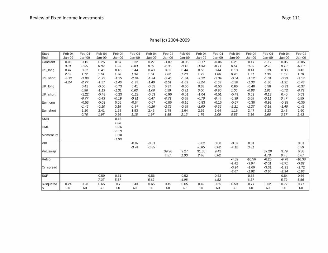
Review of Fixed Income Investments Page 111
Panel (c) 2004-2009
Start Feb-04 Feb-04 Feb-04 Feb-04 Feb-04 Feb-04 Feb-04 Feb-04 Feb-04 Feb-04 Feb-04 Feb-04 Feb-04 Feb-04 Feb-04End Jan-09 Jan-09 Jan-09 Jan-09 Jan-09 Jan-09 Jan-09 Jan-09 Jan-09 Jan-09 Jan-09 Jan-09 Jan-09 Jan-09 Jan-09Constant 0.00 0.15 0.25 0.37 0.32 0.27 -1.07 -0.05 -0.77 -0.06 0.21 0.17 -1.12 0.05 -0.05
0.01 0.35 0.82 1.23 0.83 0.87 -2.35 -0.12 -1.34 -0.11 0.61 0.65 -2.75 0.13 -0.13US_long 0.47 0.62 0.41 0.45 0.44 0.40 0.62 0.44 0.56 0.44 0.13 0.41 0.39 0.38 0.43
2.62 1.72 1.61 1.78 1.34 1.54 2.02 1.70 1.79 1.66 0.40 1.71 1.36 1.69 1.78US_short -3.12 -3.08 -1.29 -1.15 -2.04 -1.24 -2.41 -1.34 -2.22 -1.34 -0.54 -1.12 -1.31 -0.99 -1.17
-4.24 -2.77 -1.57 -1.46 -1.97 -1.49 -2.51 -1.63 -2.24 -1.59 -0.50 -1.38 -1.36 -1.31 -1.43UK_long 0.41 -0.60 -0.73 0.41 -0.55 0.37 -0.50 0.38 -0.50 0.60 -0.40 0.56 -0.33 -0.37
0.56 -1.13 -1.31 0.63 -1.00 0.59 -0.91 0.60 -0.90 1.05 -0.88 1.01 -0.72 -0.79UK_short -1.22 -0.48 -0.23 -1.29 -0.53 -0.96 -0.51 -1.04 -0.51 -0.49 0.52 -0.13 0.45 0.53
-0.77 -0.43 -0.19 -0.91 -0.47 -0.71 -0.45 -0.76 -0.44 -0.39 0.55 -0.11 0.47 0.55Eur_long -0.53 -0.03 0.05 -0.64 -0.07 -0.86 -0.16 -0.83 -0.16 -0.67 -0.30 -0.93 -0.35 -0.36
-1.45 -0.10 0.18 -1.97 -0.26 -2.72 -0.55 -2.60 -0.55 -2.21 -1.27 -3.18 -1.40 -1.42Eur_short 1.20 2.41 1.28 1.83 2.43 2.78 2.64 2.66 2.64 1.16 2.47 2.23 2.48 2.60
0.70 1.97 0.96 1.18 1.97 1.85 2.12 1.76 2.09 0.85 2.36 1.66 2.37 2.43SMB 0.15
1.08HML -0.26
-2.18Momentum -0.18
-1.99VIX -0.07 -0.01 -0.02 0.00 -0.07 0.01 0.01
-3.74 -0.55 -0.85 0.02 -4.12 0.31 0.59Vol_swap 39.26 9.27 31.36 9.42 37.20 3.79 6.38
4.57 1.00 2.48 0.82 4.78 0.45 0.67Refco -4.82 -10.56 -6.26 -9.78 -10.38
-1.42 -3.94 -2.01 -3.91 -3.82Cr_spread -3.94 -1.69 -3.31 -1.91 -1.72
-3.67 -1.92 -3.30 -2.34 -1.95S&P 0.59 0.51 0.56 0.52 0.52 0.58 0.54 0.56
7.37 5.57 5.62 4.98 4.82 6.37 5.79 5.56R-squared 0.24 0.28 0.65 0.7 0.43 0.65 0.49 0.65 0.49 0.65 0.59 0.77 0.62 0.77 0.77N 60 60 60 60 60 60 60 60 60 60 60 60 60 60 60

Review of Fixed Income Investments Page 112
Table 16 Regression of Active returns on Factors
Panel (a): 1998-2010
Start Jan-98 Jan-98 Jan-98 Jan-98 Jan-98 Jan-98 Jan-98 Jan-98 Jan-98 Jan-98 Jan-98 Jan-98 Jan-98 Jan-98End Sep-10 Sep-10 Jun-10 Sep-10 Sep-10 Mar-10 Mar-10 Mar-10 Mar-10 May-10 May-10 Mar-10 Mar-10 Mar-10Constant 0.04 0.03 0.01 0.04 0.03 -0.08 -0.06 -0.07 -0.07 0.03 0.02 -0.07 -0.05 -0.07
1.47 1.00 0.45 1.44 1.01 -2.12 -1.51 -1.75 -1.77 1.17 0.68 -1.93 -1.25 -1.70US_long 0.01 0.00 0.00 0.01 0.00 0.00 -0.01 0.00 -0.01 0.01 0.00 0.00 -0.01 -0.01
0.80 0.26 -0.21 0.48 0.25 -0.15 -0.51 -0.18 -0.48 0.33 -0.11 -0.28 -0.72 -0.67US_short -0.17 -0.09 -0.06 -0.11 -0.09 -0.06 -0.02 -0.05 -0.03 -0.05 0.00 0.00 0.05 0.04
-2.66 -1.40 -0.89 -1.75 -1.35 -0.86 -0.31 -0.77 -0.38 -0.66 -0.01 0.05 0.74 0.64UK_long
UK_short
Eur_long
Eur_short
SMB 0.012.00
HML 0.023.25
Momentum 0.00-0.95
VIX 0.00 0.00 0.00 0.00 0.00 0.00 0.00-2.87 -0.15 -0.54 1.03 -2.03 0.67 1.59
Vol_swap 3.18 2.22 2.94 2.57 2.76 1.71 2.204.54 3.01 3.52 3.17 3.98 2.36 2.80
Refco -0.80 -0.87 -0.77 -0.80 -0.87-2.63 -3.02 -2.57 -2.76 -3.01
Cr_spread -0.24 -0.25 -0.22 -0.24 -0.24-2.31 -2.64 -2.17 -2.53 -2.56
S&P 0.03 0.03 0.03 0.02 0.02 0.03 0.02 0.034.90 4.32 3.85 3.26 3.38 4.29 3.62 3.96
R-squared 0.07 0.20 0.27 0.12 0.2 0.19 0.24 0.19 0.25 0.18 0.28 0.24 0.31 0.32N 153 153 150 153 153 147 147 147 147 149 149 147 147 147

Review of Fixed Income Investments Page 113
Panel (b): 1998 – 2002
Start Jan-98 Jan-98 Jan-98 Jan-98 Jan-98 Jan-98 Jan-98 Jan-98 Jan-98 Jan-98 Jan-98 Jan-98 Jan-98 Jan-98End Dec-02 Dec-02 Dec-02 Dec-02 Dec-02 Dec-02 Dec-02 Dec-02 Dec-02 Dec-02 Dec-02 Dec-02 Dec-02 Dec-02Constant 0.02 0.02 0.01 0.02 0.02 0.01 0.00 0.01 0.01 0.02 0.02 0.01 0.00 0.01
1.26 1.26 0.99 1.23 1.29 0.31 0.23 0.36 0.35 1.21 1.28 0.31 0.23 0.36US_long 0.00 0.00 0.00 0.00 0.00 0.00 0.00 0.00 0.00 0.00 0.00 0.00 0.00 0.00
0.21 0.21 -0.01 0.32 0.40 0.13 0.10 0.18 0.26 0.29 0.42 0.10 0.06 0.30US_short -0.01 -0.01 -0.01 -0.01 -0.02 0.00 -0.01 0.00 -0.01 -0.01 -0.02 0.00 0.00 -0.01
-0.45 -0.49 -0.16 -0.38 -0.53 -0.15 -0.23 -0.15 -0.30 -0.30 -0.49 -0.08 -0.12 -0.33UK_long
UK_short
Eur_long
Eur_short
SMB 0.000.97
HML 0.000.66
Momentum 0.00-0.12
VIX 0.00 0.00 0.00 0.00 0.00 0.00 0.00-0.57 -0.90 -0.25 -0.67 -0.51 -0.85 -0.66
Vol_swap 0.28 0.33 0.25 0.28 0.27 0.33 0.280.91 1.02 0.74 0.83 0.86 0.98 0.82
Refco -0.03 -0.02 -0.03 -0.03 -0.01-0.13 -0.09 -0.16 -0.18 -0.07
Cr_spread 0.00 0.01 -0.01 -0.01 0.010.01 0.14 -0.07 -0.12 0.16
S&P 0.00 0.00 0.00 0.00 0.00 0.00 0.00 0.00-0.22 0.22 -0.73 -0.53 -0.81 -0.72 -0.53 -0.81
R-squared 0.00 0.01 0.02 0.01 0.02 0.02 0.02 0.02 0.03 0.01 0.02 0.02 0.02 0.03N 60 60 60 60 60 60 60 60 60 60 60 60 60 60

Review of Fixed Income Investments Page 114
Panel (c): Jan 2003 – Jun 2007
Start Jan-03 Jan-03 Jan-03 Jan-03 Jan-03 Jan-03 Jan-03 Jan-03 Jan-03 Jan-03 Jan-03 Jan-03 Jan-03 Jan-03End Jun-07 Jun-07 Jun-07 Jun-07 Jun-07 Jun-07 Jun-07 Jun-07 Jun-07 Jun-07 Jun-07 Jun-07 Jun-07 Jun-07Constant 0.03 0.03 0.02 0.03 0.02 0.03 0.03 0.03 0.03 0.02 0.02 0.03 0.03 0.03
5.68 5.24 4.19 5.63 4.51 4.63 4.69 3.47 3.34 5.33 4.44 4.45 4.56 3.25US_long 0.01 0.01 0.00 0.01 0.01 0.01 0.01 0.01 0.01 0.01 0.01 0.01 0.01 0.01
1.63 1.61 1.31 1.82 1.89 1.81 1.81 1.82 1.91 2.12 2.32 2.11 2.28 2.34US_short -0.04 -0.04 -0.04 -0.04 -0.05 -0.04 -0.04 -0.04 -0.05 -0.05 -0.06 -0.05 -0.06 -0.06
-2.25 -2.22 -2.13 -2.47 -2.57 -2.43 -2.42 -2.42 -2.54 -2.53 -2.74 -2.47 -2.64 -2.73UK_long
UK_short
Eur_long
Eur_short
SMB 0.000.5
HML 0.012.32
Momentum 0.00-0.89
VIX 0.00 0.00 0.00 0.00 0.00 0.00 0.001.1 1.46 0.35 0.80 0.97 1.41 0.79
Vol_swap -0.16 -0.23 -0.12 -0.16 -0.14 -0.22 -0.15-1.25 -1.51 -0.68 -0.89 -1.09 -1.44 -0.83
Refco -0.22 -0.20 -0.21 -0.20 -0.20-1.92 -1.75 -1.89 -1.70 -1.70
Cr_spread 0.01 0.03 0.01 0.03 0.030.10 0.49 0.15 0.55 0.52
S&P 0.00 0.00 0.00 0.00 0.00 0.00 0.00 0.000.04 -0.12 0.96 0.86 1.12 1.06 0.98 1.21
R-squared 0.1 0.1 0.2 0.12 0.14 0.13 0.14 0.13 0.15 0.19 0.21 0.2 0.21 0.22N 54 54 54 54 54 54 54 54 54 54 54 54 54 54

Review of Fixed Income Investments Page 115
Panel (d): 2007 – 2010
Start Jul-07 Jul-07 Jul-07 Jul-07 Jul-07 Jul-07 Jul-07 Jul-07 Jul-07 Jul-07 Jul-07 Jul-07 Jul-07 Jul-07End Sep-10 Sep-10 Jun-10 Sep-10 Sep-10 Mar-10 Mar-10 Mar-10 Mar-10 May-10 May-10 Mar-10 Mar-10 Mar-10Constant 0.17 0.14 0.15 0.16 0.14 -0.19 -0.12 -0.19 -0.16 0.12 0.09 -0.21 -0.14 -0.18
1.43 1.34 1.22 1.37 1.32 -1.31 -0.92 -1.24 -1.19 0.93 0.83 -1.41 -1.08 -1.28US_long 0.03 0.01 0.01 0.00 0.00 -0.02 -0.04 -0.02 -0.02 -0.01 -0.01 -0.02 -0.04 -0.03
0.65 0.16 0.34 0.09 0.1 -0.45 -0.97 -0.38 -0.64 -0.14 -0.34 -0.52 -1.14 -0.73US_short -0.46 -0.28 -0.34 -0.29 -0.27 -0.05 0.01 -0.06 -0.03 -0.13 -0.05 0.05 0.16 0.11
-2.41 -1.7 -1.57 -1.47 -1.52 -0.27 0.03 -0.29 -0.16 -0.52 -0.25 0.20 0.78 0.51UK_long
UK_short
Eur_long
Eur_short
SMB -0.02-0.32
HML 0.020.46
Momentum -0.02-1.24
VIX -0.01 0.00 0.00 0.01 -0.01 0.00 0.01-2.29 -0.29 0.11 0.98 -1.85 -0.16 0.93
Vol_swap 9.02 6.42 9.25 7.99 8.97 5.91 7.254.1 2.87 3.05 2.90 3.79 2.53 2.64
Refco -0.28 -0.58 -0.16 -0.34 -0.54-0.35 -0.82 -0.23 -0.55 -0.83
Cr_spread -0.26 -0.30 -0.22 -0.31 -0.28-1.08 -1.42 -1.03 -1.65 -1.45
S&P 0.05 0.04 0.05 0.04 0.04 0.06 0.04 0.054 2.19 3.03 2.63 2.80 3.24 2.95 3.08
R-squared 0.18 0.44 0.48 0.29 0.44 0.48 0.58 0.48 0.6 0.32 0.5 0.5 0.63 0.64N 39 39 36 39 39 33 33 33 33 35 35 33 33 33

Review of Fixed Income Investments Page 116
Table 17
Regression of benchmark difference (GPFG_BM minus Barclays Global Aggregate) on factors: 1998 – 2010
Start_dt Jan-98 Jan-98 Jan-98 Jan-98 Jan-98 Jan-98 Jan-98 Jan-98 Jan-98 Jan-98 Jan-98 Jan-98 Jan-98 Jan-98End_dt Sep-10 Sep-10 Jun-10 Sep-10 Sep-10 Mar-10 Mar-10 Mar-10 Mar-10 May-10 May-10 Mar-10 Mar-10 Mar-10Constant -0.06 -0.06 -0.06 -0.06 -0.06 -0.06 -0.06 -0.07 -0.07 -0.06 -0.06 -0.05 -0.05 -0.06
-3.30 -3.38 -3.28 -3.31 -3.35 -2.54 -2.54 -2.64 -2.63 -3.40 -3.38 -2.23 -2.23 -2.51US_long 0.06 0.06 0.07 0.06 0.06 0.07 0.07 0.07 0.07 0.07 0.07 0.07 0.07 0.07
6.48 6.32 6.57 6.34 6.28 7.52 7.49 7.55 7.49 7.49 7.41 7.81 7.76 7.81US_short -0.07 -0.06 -0.09 -0.06 -0.06 -0.09 -0.09 -0.09 -0.09 -0.09 -0.09 -0.09 -0.09 -0.10
-1.81 -1.49 -2.08 -1.51 -1.43 -2.15 -2.16 -2.24 -2.21 -2.03 -1.96 -2.09 -2.09 -2.17UK_long
UK_short
Eur_long
Eur_short
SMB 0.00-0.72
HML 0.000.68
Momentum -0.01-1.69
VIX 0.00 0.00 0.00 0.00 0.00 0.00 0.00-0.72 -0.25 0.78 0.71 0.51 0.52 1.22
Vol_swap 0.17 0.23 0.38 0.38 -0.03 0.02 0.260.42 0.51 0.77 0.76 -0.07 0.05 0.52
Refco -0.56 -0.56 -0.49 -0.49 -0.53-3.12 -3.11 -2.74 -2.73 -2.90
Cr_spread 0.00 0.00 0.01 0.01 0.010.07 0.06 0.16 0.18 0.16
S&P 0.00 0.00 0.00 0.00 0.00 0.00 0.00 0.000.88 -0.21 0.56 -0.31 0.04 0.19 -0.28 0.32
R-squared 0.30 0.31 0.34 0.31 0.31 0.39 0.39 0.39 0.39 0.39 0.39 0.42 0.42 0.43N 153 153 150 153 153 147 147 147 147 149 149 147 147 147

Review of Fixed Income Investments Page 117
File: Fixed_Income_Project_Final_Report_29_March_2011.doc