nmr study of lithium mobility in polymer electrolytes
TRANSCRIPT

NMR study of lithium mobility in polymer electrolytes
Tan-Vu Huynh
To cite this version:
Tan-Vu Huynh. NMR study of lithium mobility in polymer electrolytes. Polymers. Universited’Orleans, 2015. English. <NNT : 2015ORLE2054>. <tel-01362053>
HAL Id: tel-01362053
https://tel.archives-ouvertes.fr/tel-01362053
Submitted on 8 Sep 2016
HAL is a multi-disciplinary open accessarchive for the deposit and dissemination of sci-entific research documents, whether they are pub-lished or not. The documents may come fromteaching and research institutions in France orabroad, or from public or private research centers.
L’archive ouverte pluridisciplinaire HAL, estdestinee au depot et a la diffusion de documentsscientifiques de niveau recherche, publies ou non,emanant des etablissements d’enseignement et derecherche francais ou etrangers, des laboratoirespublics ou prives.

UNIVERSITE D’ORLEANS
ECOLE DOCTORALE
ENERGIE, MATERIAUX, SCIENCES DE LA TERRE ET DE
L’UNIVERS
Laboratoire CNRS UPR 3079 Conditions Extremes et Materiaux :
Haute Temperature et Irradiation
THESE presentee par :
Tan-Vu HUYNH
soutenue le : 4 Novembre 2015
pour obtenir le grade de : Docteur de l’universite d’Orleans
Discipline/ Specialite: Chimie
Etude par Resonance Magnetique Nucleaire
de la mobilite du lithium
dans les electrolytes a base de polymeres
THESE dirigee par :
Michael Deschamps Professeur, Universite d’Orleans
RAPPORTEURS :
Daniel ABERGEL Directeur de Recherche, Ecole NormaleSuperieure, Paris
Anne-Laure ROLLET Chargee de Recherches HDR, Universite Pierreet Marie Curie, Paris
JURY :
Renaud BOUCHET Professeur, Institut Polytechnique de GrenobleFrancois TRAN VAN Professeur, Universite de ToursMichael DESCHAMPS Professeur, Universite d’Orleans

1


Abstract
Nuclear magnetic resonance (NMR) spectroscopy is well known as a powerful tool
to study molecular structure and dynamics. In battery materials, the mobility of
lithium cations is especially important as it is the key to the limitations in battery
power and charging rates. NMR spectroscopy can give access to self-diffusion co-
efficients of spin bearing species using pulsed field gradients which measure atomic
displacement over 1-2 µm length scales. The relaxation of nuclear spins at high
magnetic fields, on the other hand, is governed by fluctuations of NMR interac-
tions resonant with the Larmor frequency, at the nanosecond timescale, and these
are usually related to atomic motions over 0.1 - 1 nm.
In this thesis, we recorded self-diffusion coefficients and 7Li relaxation rates for
two polymer electrolytes: LiTFSI in polyethylene oxide (PEO) and in a block-
copolymer PS-PEO(LiTFSI)-PS. We first investigated the effect of magic-angle
spinning (MAS) on diffusion and relaxation, showing that MAS can help retrieve
diffusion coefficient when relaxation is fast and diffusion is slow, and second, that
lithium motion is not perturbed by the partial alignment of PEO under MAS in-
duced pressure. The relaxation rates of 7Li were measured at three high magnetic
fields (4.7, 9.4 and 17.6 Tesla) allowing us to perform a simple relaxometry study
of Li+ motion at the nanosecond timescale. In order to reproduce the transverse
and longitudinal relaxation behaviors, it proved necessary to introduce a simple
model with two correlation times. It showed for the first time that the lithium
dynamics in PS-PEO(LiTFSI)-PS is slowed down by the presence of PS domains
compared to the pure PEO with similar chain lengths. The results are analyzed
and compared to other studies based on molecular dynamics or physical models
of diffusion in polymers.
A second series of gel polymer electrolytes based on poly(vinylidene fluoride-
co-hexafluoropropylene) (PVdF-HFP), PEGM (Poly ethyleneglycol methyl ether
methacrylate)/PEGDM (Poly ethyleneglycol dimethacrylate), and LiTFSI in ionic
liquids were also studied. Adding oxygenated polymers to increase the retention of
ionic liquids slowed the diffusion down and explained why the battery performance
was degraded at higher charging rates.

Acknowledgements
This works was carried out in the laboratory Conditions Extrêmes et Matéri-
aux : Haute Température et Irradiation (CEMHTI)-UPR3079 CNRS, Université
d’Orléans, under the direction of Prof. Michaël Deschamps.
I would like to thank Prof. Michaël Deschamps for proposing me this subject,
giving a chance to study in NMR world. He has aroused me about the inspiration
of science. I would like to thank him also about his kindness, his time to guide
me to finish this thesis.
I would like to thank Dr. Robert Messinger for teaching me about NMR ex-
periments, helping me to learn NMR theory, accompanying me throughout my
research work sympathetically.
I would like to thank Dr. Vincent Sarou-Kanian for helping to set up NMR experi-
ments, solving out technical problems, sharing his knowledge about NMR. I would
like to thank also Dr. Catherine Bessada, director of CEMHTI, for welcoming me
for three years.
I would like to thank Prof. Renaud Bouchet from the laboratory of Electrochimie
et de Physicochimie des Matériaux et des Interfaces (LEPMI) and Victor Chau-
doy from the laboratory Physico-Chime des Matériaux et des Electrolytes pour
l’Energie (PCM2E). They have provided me the materials that were used in this
thesis. Thank you a lot for spending your time on discussing about my works.
I would like to thank the jury for reading and correcting my thesis.
A big thank for all peoples working in CEMHTI, for your kindness. Finally, I
extend my gratitude to my family in Vietnam, my dear parents, my brother, and
my girlfriend who encouraged and supported me.
ii

Contents
Abstract i
Acknowledgements ii
Contents iii
Resumé de la thèse en français vii
1. Les électrolytes à base de polymères . . . . . . . . . . . . . . . . . . vii2. Introduction de Résonance Mangetique Nucléaire . . . . . . . . . . ix3. L’influence de la rotation à l’angle magique (MAS) sur les expéri-
ences de RMN dans les électrolytes polymères . . . . . . . . . . . . x4. Caractérisation des temps de relaxation et des coefficients de diffusion xi5. Les électrolytes polymères à base de PVdF-HFP . . . . . . . . . . . xii6. Conclusions et perspectives . . . . . . . . . . . . . . . . . . . . . . . xiv
1 Lithium metal battery 1
1.1 Lithium metal battery . . . . . . . . . . . . . . . . . . . . . . . . . 11.2 Ultra-thin lithium metal battery . . . . . . . . . . . . . . . . . . . . 31.3 Solid polymer electrolytes . . . . . . . . . . . . . . . . . . . . . . . 41.4 Ion motion mechanisms . . . . . . . . . . . . . . . . . . . . . . . . . 51.5 Materials . . . . . . . . . . . . . . . . . . . . . . . . . . . . . . . . 91.6 Difficulties in studying polymer electrolytes . . . . . . . . . . . . . . 10
2 Introduction to Nuclear Magnetic Resonance 13
2.1 Introduction to NMR . . . . . . . . . . . . . . . . . . . . . . . . . . 132.1.1 The Hamiltonians . . . . . . . . . . . . . . . . . . . . . . . . 132.1.2 Spin angular momentum operators . . . . . . . . . . . . . . 142.1.3 Zeeman interaction . . . . . . . . . . . . . . . . . . . . . . . 152.1.4 Chemical shift . . . . . . . . . . . . . . . . . . . . . . . . . . 152.1.5 Dipolar interaction . . . . . . . . . . . . . . . . . . . . . . . 162.1.6 Quadrupolar interaction . . . . . . . . . . . . . . . . . . . . 17
2.2 Relaxation of nuclear spins to study molecular motion . . . . . . . . 192.2.1 Longitudinal relaxation time T1 . . . . . . . . . . . . . . . . 202.2.2 Transverse relaxation time T2 . . . . . . . . . . . . . . . . . 20
iii

Contents iv
2.2.3 Molecular vibrations . . . . . . . . . . . . . . . . . . . . . . 212.2.4 Molecular flexibility . . . . . . . . . . . . . . . . . . . . . . . 212.2.5 Molecular rotations . . . . . . . . . . . . . . . . . . . . . . . 22
2.3 How to study molecular motions with relaxation times . . . . . . . 222.3.1 Angular dependent NMR interactions . . . . . . . . . . . . . 222.3.2 Auto-correlation functions . . . . . . . . . . . . . . . . . . . 232.3.3 Determination of the spectral density . . . . . . . . . . . . . 252.3.4 Spectral densities . . . . . . . . . . . . . . . . . . . . . . . . 25
2.3.4.1 Bloembergen-Purcell-Pound (BPP) model . . . . . 262.3.4.2 Cole-Davidson function . . . . . . . . . . . . . . . 262.3.4.3 Lipari-Szabo model . . . . . . . . . . . . . . . . . . 26
2.4 Diffusion . . . . . . . . . . . . . . . . . . . . . . . . . . . . . . . . . 272.4.1 Fick’s laws . . . . . . . . . . . . . . . . . . . . . . . . . . . . 282.4.2 Self-Diffusion . . . . . . . . . . . . . . . . . . . . . . . . . . 29
2.4.2.1 Introduction . . . . . . . . . . . . . . . . . . . . . 292.4.2.2 Stokes-Einstein equation . . . . . . . . . . . . . . . 302.4.2.3 Random walk theory . . . . . . . . . . . . . . . . . 302.4.2.4 Diffusion propagators . . . . . . . . . . . . . . . . 31
2.4.3 Conductivity and diffusion . . . . . . . . . . . . . . . . . . . 322.4.3.1 Mobility of Ions . . . . . . . . . . . . . . . . . . . . 322.4.3.2 Nernst-Einstein equation . . . . . . . . . . . . . . . 33
2.4.4 Diffusion coefficient measurements by NMR . . . . . . . . . 33
3 The Effect of Magic Angle Spinning on Relaxation and Diffusion 39
3.1 Magic angle spinning . . . . . . . . . . . . . . . . . . . . . . . . . . 393.2 Temperature calibration . . . . . . . . . . . . . . . . . . . . . . . . 403.3 Observation . . . . . . . . . . . . . . . . . . . . . . . . . . . . . . . 403.4 Previous studies . . . . . . . . . . . . . . . . . . . . . . . . . . . . . 423.5 Polymer state control . . . . . . . . . . . . . . . . . . . . . . . . . . 443.6 Diffusion and relaxation time results . . . . . . . . . . . . . . . . . 473.7 Conclusion . . . . . . . . . . . . . . . . . . . . . . . . . . . . . . . . 50
4 Relaxation times and diffusion coefficient measurement 51
4.1 Introduction . . . . . . . . . . . . . . . . . . . . . . . . . . . . . . . 514.2 Diffusion coefficient and conductivity of polymer samples . . . . . . 534.3 Relaxation rates R1 and R2 characterization . . . . . . . . . . . . . 60
4.3.1 Calculation of relaxation rates . . . . . . . . . . . . . . . . . 604.3.2 Simple models: Bloembergen–Purcell–Pound (BPP) and Cole-
Davidson function . . . . . . . . . . . . . . . . . . . . . . . 624.3.2.1
⟨
C2Q
⟩
variation . . . . . . . . . . . . . . . . . . . . 644.3.2.2 Dipolar Relaxation term RDD . . . . . . . . . . . . 66
4.3.3 Multi-exponentials correlation function . . . . . . . . . . . . 684.4 Conclusion . . . . . . . . . . . . . . . . . . . . . . . . . . . . . . . . 79
5 Polymer electrolytes in ultra thin film battery 81

Contents v
5.1 Introduction . . . . . . . . . . . . . . . . . . . . . . . . . . . . . . . 815.2 Experiments . . . . . . . . . . . . . . . . . . . . . . . . . . . . . . . 835.3 Results and discussions . . . . . . . . . . . . . . . . . . . . . . . . . 835.4 Conclusions . . . . . . . . . . . . . . . . . . . . . . . . . . . . . . . 90
6 Conclusions and Perspectives 91
6.1 Conclusions . . . . . . . . . . . . . . . . . . . . . . . . . . . . . . . 916.2 Perspectives . . . . . . . . . . . . . . . . . . . . . . . . . . . . . . . 92
A Experimental relaxation rates and calculated parameters 93
A.1 Calculation method . . . . . . . . . . . . . . . . . . . . . . . . . . . 93A.2 Experimental relaxation rates . . . . . . . . . . . . . . . . . . . . . 94A.3 The parameters calculated from successful model . . . . . . . . . . 97
Bibliography 99


Resumé vii
Resumé de la thèse en français
1. Les électrolytes à base de polymères
L’accumulateur lithium-métal-polymère (LMP) possède une grande capacité et une ten-
sion plus élevée grâce à l’utilisation de l’anode en lithium métallique. Cependant, les
risques d’incendie et d’explosion limitent l’application de ces types de batteries au quo-
tidien. Ces désavantages viennent de la formation de dendrites de lithium métallique
pendant la charge causant des court-circuits. Les électrolytes liquides sont inflammables
et peuvent réagir avec les électrodes actives (principalement le lithium métal). Par contre,
les électrolytes à base de polymères comme le polyoxyde d’éthylène (PEO) sont de bons
candidats pour une utilisation dans les batteries lithium-métal (comme dans la Bluecar
d’Autolib...). Deux problèmes sont néanmoins observés dans ces électrolytes: d’abord, la
conductivité est plus basse que dans un électrolyte liquide conventionnel, et deuxièmement,
leur résistance mécanique est faible et n’empêche pas forcément la formation de dendrites
au cours de la charge. Donc, les copolymères à bloc dérivés du PEO et renforcés par des
blocs de polystyrène (PS) [1] ont été développés pour augmenter la résistance à la forma-
tion de dendrites. La figure 1 montre le composition des électrolytes polymères étudiés
dans chapitres 3 et 4.
CH2 CH2 On
CH2 CHp
CH2CHp CF3
O=S=O
N- Li+
CF3
O=S=O
CH2 CH2 OnCF3
O=S=O
N- Li+
CF3
O=S=O
PEO(LiTFSI) PS-PEO(LiTFSI)-PS
Figure 1: La structure des électrolytes polymères étudiés: PEO(LiTFSI) etPS-PEO(LiTFSI)-PS
L’utilisation de la relaxation et de la diffusion vont ainsi permettre de mieux appréhen-
der l’effet des blocs de PS sur la dynamique du Li+ dans les domaines de PEO. Dans
un deuxième temps, un autre type d’électrolyte a aussi été étudié: ils sont réalisés à base
de PVdF-HFP -poly(vinylidène fluoride-co-hexafluoropropylène)- sous forme de gels. Ces
électrolytes sont utilisés dans des batteries ultra-fines à la place du LIPON (pour oxynitrure
de lithium et de phosphore LixPOyNz) en raison de leur coût plus faible. Le sel de LiTFSI
est ici solubilisé dans un liquide ionique (IL) Pyr13FSI(N-methyl-N-propylpyrrolidinium
bis(fluorosulfonyl)imide) mélangé avec le polymère pour avoir une conductivité plus élevée.

Resumé viii
PVdF-HFP
Figure 2: Echantillon PH: la solution de LiTFSI dans Pyr13FSI est mélangéeavec le PVdF-HFP (©Victor Chaudoy - Université de Tours).
PEGDM network
Cross-linked node
PEGM pendant chain
Permit to increase mobility
Figure 3: Echantillon POE: l’électrolyte (LiTFSI dans le Pyr13FSI) estmélangé avec un polymère PEGDM/PEGM (©Victor Chaudoy - Université de
Tours)
PEGDM network
Cross-linked node
PVdF-HFP
PEGM pendant chain
Permit to increase mobility
Figure 4: Echantillon SRIP: Le polymère est un mélange de PVdF-HFP etde PEGM/PEGDM -sans lien chimique entre eux-, avec le même électrolyte
(©Victor Chaudoy - Université de Tours).

Resumé ix
Cependant, les membranes poreuses de PVdF-HFP retiennent faiblement le liquide ion-
ique à température plus élevée (60 ) ce qui cause une perte de IL lorsque le système
est assemblé. L’utilisation de polymères de type PEGM (Poly ethyleneglycol methyl ether
methacrylate)/PEGDM (Poly ethyleneglycol dimethacrylate) permet d’améliorer la réten-
tion de l’électrolyte mais diminue malheureusement la vitesse de diffusion du lithium par
interaction de celui-ci avec le polymère ajouté. Les polymères étudiés sont décrits dans les
figures ci-dessus.
2. Introduction de Résonance Mangetique Nucléaire
Dans cette section, nous présenterons les principes de la Résonance Magnétique Nucléaire
(RMN) et les différentes méthodes expérimentales utilisées dans cette thèse. Le principal
avantage de la spectroscopie RMN réside dans sa capacité à fournir des informations sur
la structure (distances ou angles de liaisons) et la dynamique des molécules (relaxation
ou diffusion). Dans le cadre de cette étude, la RMN vient compléter les informations
données par les mesures de conductivité. La conductivité est une paramètre important
dans l’étude des matériaux électrolytes solides comme les polymères, et elle est étroitement
liée à la diffusion des cations et des anions dans l’électrolyte. L’utilisation de gradient
de champs magnétiques "pulsés" (PFG) donne accès aux coefficients d’auto-diffusion des
espèces portant un spin nucléaire détectable. Les coefficients d’auto-diffusion mesurés
valent entre 10−10 et 10−13 m2/s, et les déplacements spatiaux des ions sont mesurées sur
des temps variant de 1 ms (pour les espèces rapides) à 1 s (pour les espèces diffusant plus
lentement), ce qui correspond à des déplacements ioniques de quelques µm pour la mesure
du coefficient d’auto-diffusion. La mesure de la conductivité (plus simple dans sa mise en
oeuvre) ne peut mesurer que la somme des contributions de toutes les espèces chargés.
Ces deux techniques, ensemble, peuvent se compléter utilement pour étudier le mécanisme
de transport dans les électrolytes à base de polymère. [2] Cependant, elles ne peuvent
donner qu’une description macroscopique à l’échelle du micromètre. La complexité des
phénomènes en jeu montre que ces mesures ne suffisent pas pour comprendre parfaitement
la mobilité des cations comme le Li+, qui est cruciale pour améliorer la vitesse de charge
des batteries au lithium. La mobilité des molécules peut être étudiée via les processus
de relaxation (ou de retour à l’équilibre des états de spins) qui sont liés aux fluctuations
des interactions des spins avec leur environnement ayant lieu à des fréquences jusqu’à la
fréquence de Larmor (soit quelques centaines de MHz).
Dans cette thèse, nous avons ainsi combiné ces deux types d’étude afin de mieux com-
prendre la mobilité des ions lithium dans les électrolytes à base de polymères.
Resumé x
10 8 6 0
1H ref TMS
10 8 6 0 ppm
97 °C
10 kHz
1 hour
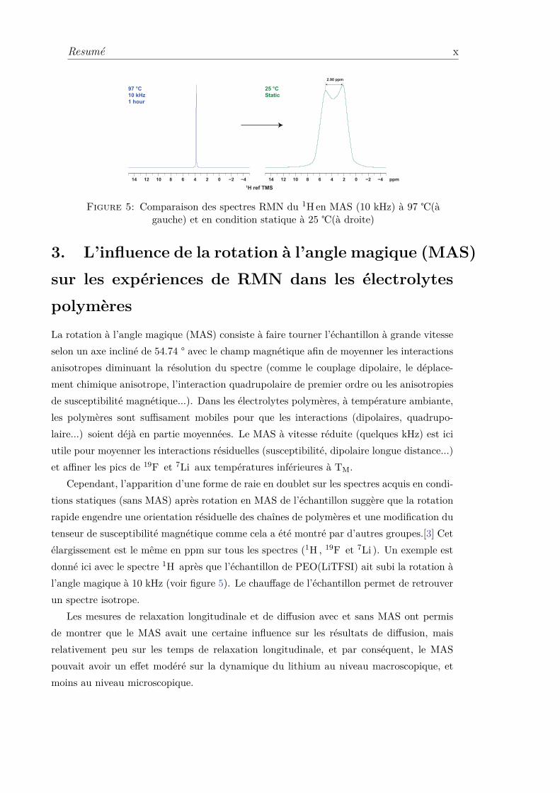
Static
Figure 5: Comparaison des spectres RMN du 1H en MAS (10 kHz) à 97 (àgauche) et en condition statique à 25 (à droite)
3. L’influence de la rotation à l’angle magique (MAS)
sur les expériences de RMN dans les électrolytes
polymères
La rotation à l’angle magique (MAS) consiste à faire tourner l’échantillon à grande vitesse
selon un axe incliné de 54.74 ° avec le champ magnétique afin de moyenner les interactions
anisotropes diminuant la résolution du spectre (comme le couplage dipolaire, le déplace-
ment chimique anisotrope, l’interaction quadrupolaire de premier ordre ou les anisotropies
de susceptibilité magnétique...). Dans les électrolytes polymères, à température ambiante,
les polymères sont suffisament mobiles pour que les interactions (dipolaires, quadrupo-
laire...) soient déjà en partie moyennées. Le MAS à vitesse réduite (quelques kHz) est ici
utile pour moyenner les interactions résiduelles (susceptibilité, dipolaire longue distance...)
et affiner les pics de 19F et 7Li aux températures inférieures à TM.
Cependant, l’apparition d’une forme de raie en doublet sur les spectres acquis en condi-
tions statiques (sans MAS) après rotation en MAS de l’échantillon suggère que la rotation
rapide engendre une orientation résiduelle des chaînes de polymères et une modification du
tenseur de susceptibilité magnétique comme cela a été montré par d’autres groupes.[3] Cet
élargissement est le même en ppm sur tous les spectres (1H , 19F et 7Li ). Un exemple est
donné ici avec le spectre 1H après que l’échantillon de PEO(LiTFSI) ait subi la rotation à
l’angle magique à 10 kHz (voir figure 5). Le chauffage de l’échantillon permet de retrouver
un spectre isotrope.
Les mesures de relaxation longitudinale et de diffusion avec et sans MAS ont permis
de montrer que le MAS avait une certaine influence sur les résultats de diffusion, mais
relativement peu sur les temps de relaxation longitudinale, et par conséquent, le MAS
pouvait avoir un effet modéré sur la dynamique du lithium au niveau macroscopique, et
moins au niveau microscopique.

Resumé xi
100 80 60 40 20
2.6 2.8 3 3.2 3.4
10-13
10-12
10-11
10-10
1013
1012
1011
1010
Temperature, T (°C)
1000/T (K-1)
Dif
fus
ion
Co
eff
icie
nt,
D (
m2/s
) TM
TM
59.6°C
55.5°C
Figure 6: Les coefficients d’auto-diffusion de Li+( ), TFSI−(N) dansPEO(LiTFSI) et PS-PEO(LiTFSI)-PS mesurés dans un échantillon statique.Les énergies d’activation sont calculées pour les coefficients de diffusion en util-isant la loi d’Arrhenius. Les températures de fusion de PEO(LiTFSI) et PS-
PEO(LiTFSI)-PS sont estimées ici à environ 59.6 et 55.5 .
4. Caractérisation des temps de relaxation et des
coefficients de diffusion
Dans cette section, nous étudierons la mobilité du Li+ au niveau microscopique (en util-
isant les temps de relaxation) et macroscopique (avec les mesures de diffusion par PFG,
conductivité, etc...). Pour éviter les effets éventuels du MAS, nous avions choisi de réaliser
les expériences en condition statique.
La figure 6 présente les coefficients d’auto-diffusion (D) de Li+ et TFSI− dans les
polymères PEO(LiTFSI) et PS-PEO(LiTFSI)-PS. Ils ont été mesurés de telle sorte que le
libre parcours moyen λ des ions durant le temps de diffusion ∆ était d’environ 2 µm en
utilisant l’équation: λ =√
6D∆.
Nous avons mesuré les temps de relaxation longitudinale et transverse du 7Li à trois
champs magnétiques (4.7, 9.4 et 17.6 T) en fonction de la température de 25 à 100 . Nous
avons observé que la relaxation longitudinale est mono-exponentielle avec un seul temps
caractéristique T1, tandis que la relaxation transverse a un comportement bi-exponentiel
pour PEO(LiTFSI)(si T < TM ) et PS-PEO(LiTFSI)-PS(à toute température). Les temps
de relaxation longitudinale et transverse sont ensuite interprétés en utilisant le logiciel
Maple (Maple est produit par Waterloo Maple Inc.) à l’aide d’un modèle à quatre variables,
le plus simple possible, décrivant la relaxation des 7Li comme provenant principalement

Resumé xii
de l’interaction quadrupolaire et d’une perturbation d’origine dipolaire (on négligera les
termes croisés).
Brièvement, nous avons considéré que l’interaction quadrupolaire fluctue à trois dif-
férentes échelles de temps:
a. Les mouvements très rapides: la vibration du lithium ou des atomes de polymères,
qui affecte la valeur de l’interaction quadrupolaire effective⟨
C2Q
⟩
, dépendante de la
température.
b. Les fluctuations dans la sphère de coordination des ions lithium, formée par les atomes
d’oxygènes voisins: arrivée ou départ d’un oxygène, ou réorientation de l’ensemble
du polyèdre de coordination par mouvements concertés des chaînes de polymère.
Ces fluctuations vont mener à un moyennement partiel de l’interaction quadrupolaire
(décrit par le paramètre d’ordre S2) avec une échelle de temps τ1.
c. Sur une échelle de temps plus longue (τ2), le lithium s’est déplacé dans un autre envi-
ronnement dans lequel son interaction quadrupolaire a une orientation complètement
différente.
Ce modèle nous a permis d’expliquer la relaxation de Li+ dans nos électrolytes polymères.
Les paramètres obtenus après ajustement sont présentés dans la figure 7. Le point le plus
important est que nous avons prouvé le ralentissement induit par les blocs de PS sur les
mouvements microscopiques du lithium, en contradiction avec l’hypothèse communément
admise: la conductivité est identique dans le polymère homogène PEO(LiTFSI) et dans les
domaines de PEO du copolymère PS-PEO(LiTFSI)-PS.[4, 5] Ceci implique que la différence
entre coefficients de diffusion (voir figure 6) n’est pas seulement un effet "géométrique" du
à la tortuosité des domaines de PEO.
5. Les électrolytes polymères à base de PVdF-
HFP
Ce projet est une collaboration entre le laboratoire "Physico Chimie des Matériaux et des
Electrolytes pour L’Energie" (PCM2E) à Tours et le CEMHTI. Le but de ce projet était
de comprendre pourquoi l’ajout d’un polymère oxygéné a des conséquences négatives sur
la capacité des batteries ultra-fines à vitesses de charge élevées (C ou 2C soit une charge
complète en 1 heure ou 1/2 heure). Ce polymère avait pour but d’améliorer la rétention
de l’électrolyte au sein de la membrane poreuse, et même si la conductivité diminuait avec
l’ajout de polymère oxygéné, il restait à confirmer que le lithium était bien ralenti par ce
polymère (et pas seulement les autres espèces, le cation du LI et les anions).
Les coefficients de diffusion des différentes molécules des échantillons ont été mesurés.
Le coefficient de diffusion de Li+ est maximal pour une concentration de LiTFSI de x = 1.3

Resumé xiii
PEO(LiTFSI)
Temperature, T (°C)
7L
i N
MR
Re
lax
ati
on
Tim
e (
s)
7L
i N
MR
Re
lax
ati
on
Ra
te (
s-1)
1000/T (K-1)
a. b. PS-PEO(LiTFSI)-PS
R2,slow
R2,fast
R2 R
1
100 80 60 40 20
2.6 2.8 3 3.2 3.4
100
101
102
103
100
10-1
10-2
10-3
Temperature, T (°C)
7L
i N
MR
Re
lax
ati
on
Tim
e (
s)
7L
i N
MR
Re
lax
ati
on
Ra
te (
s-1)
1000/T (K-1)
100 80 60 40 20
2.6 2.8 3 3.2 3.4
100
101
102
103
100
10-1
10-2
10-3T
MT
M
59.6 °C 55.5 °C
R2,fast
R2,slow
R1
25
35
45
55
CQ2
Q2 >
(kH
z)
1000/T (K-1)
Temperature, T (°C)100 80 60 40 20
2.6 2.8 3 3.2 3.4
1000/T (K-1)
Ord
er
Para
mete
r, S
2
0
0.2
0.4
0.6
0.8
1
S2
Temperature, T (°C)100 80 60 40 20
2.6 2.8 3 3.2 3.4
100 80 60 40 20
2.6 2.8 3 3.2 3.4
100
101
102
Co
rrela
tio
n t
ime,
1 &
2 (
ns)
1000/T (K-1)
Temperature, T (°C)
Dip
ola
r R
ela
xati
on
Term
, R
DD (
Hz)
1000/T (K-1)
Temperature, T (°C)
RDD
100 80 60 40 20
2.6 2.8 3 3.2 3.4100
101
102
c.
Figure 7: a. et b. Les vitesses de relaxation R1 (partie basse de la graphique)et R2 ( partie haute du graphique) observées pour le 7Li sous trois champsmagnétiques (17.4 T, 9.4 T, 4.7 T) en fonction de la température. Les lignescontinues et pointillées représentent les courbes ajustées pour R1 et R2. La
figure (c) présente les paramètres ajustés
√
⟨
C2Q
⟩
, τ1 et τ2, S2 et RDD dans
PEO(LiTFSI)( ) et PS-PEO(LiTFSI)-PS(N). Les énergies d’activation sontcalculées pour τ1 et τ2 en utilisant la loi d’Arrhenius.

Resumé xiv
M. Les coefficients de diffusion de Li+ des échantillons SRIP sont plus faibles que dans les
échantillons sans polymère oxygéné. De plus, le ratio PEGM:PEGDM n’a pas d’effet sur
la diffusion du lithium.
La présence d’interactions entre Li+ et le polymère oxygéné est confirmée par le car-
actère bi-exponentiel de la relaxation transverse du 7Li dans les échantillons SRIP et POE
(comme cela est détaillé dans le chapitre 5).
6. Conclusions et perspectives
Dans cette thèse, nous avons cherché à caractériser la mobilité du Li+ dans les électrolytes
à base de polymère, à l’échelle du nanomètre avec la relaxation des spins nucléaires, et à
l’échelle du micromètre avec la mesure de coefficients de diffusion par gradients de chanp
pulsés. Pour pouvoir interpréter les vitesses de relaxation du 7Li , nous avons réussi à
développer une nouvelle fonction de corrélation des interactions quadrupolaires subies par
Li+ dans un polymère. Ces résultats peuvent ensuite être combinés au sein de modèle
théorique tpe "Rouse".
Dans le futur, nous pourrons aussi appliquer la même démarche sur d’autres matériaux
comme PSTFSILi-PEO-PSTFSILi. Par ailleurs, des études de dynamique moléculaires
pourront être réalisées afin d’affiner notre compréhension de la relaxation.
En parallèle, les outils développés ont pu être utilisés sur des électrolytes à base de
PVdF-HFP et nous donne des résultats très intéressants. L’ajout de polymères oxygénés
PEGM/PEGDM permet d’améliorer la rétention de l’électrolyte dans les pores de la mem-
brane, cependant, la diffusion des ions Li+ est ralenties ce qui nuit aux propriétés de la
batterie à vitesse de charge élevée.
Dans le futur, nous pourrons aussi envisager des études similaires mais en condition
in situ, de façon à prendre en compte les modifications éventuelles des polymères lors de
l’assemblage des cellules.

Chapter 1
Lithium metal battery
1.1 Lithium metal battery
The development of mobile electronic technology and the need for clean energy
storage lead to the development of battery industry. In particular, the electric
car is expected to play an important place in near future, as 27 % of the world’s
energy consumption concerns transportation.[6] Batteries which possess a high
energy density are becoming more and more necessary, as most systems do not
yet offer enough capacity to compete with fossile fuels.
Presented by Sony in 1991, the Li-ion battery is based on a graphite anode and
have been developed during more than two decades. However, their improvement
is threatened due to the theoretical performance limits of both cathode and anode
materials. [6, 7]
The use of metallic lithium as anode in batteries started in the 70s.[6] This was due
to its high theoretical specific capacity (3860 mAh/g for the anode), its lightest
weight metal (M=6.94 g/mol, ρ=0.59 g/cm3), and to its lowest negative electro-
chemical potential (-3.040 V vs the standard hydrogen electrode).[8] Moreover,
polymer electrolytes can withstand the reductive power of metallic lithium. Fig-
ure 1.2 depicts a lithium-metal polymer battery, as the one used in the Bluecar
from the Bolloré company. It must be noted that the "LiPo" batteries that are
found on the market have no polymer electrolyte and are in fact, Li-ion batteries.
However, the formation of lithium dendrites during repeated charge/discharge
cycles is still the biggest problem of this kind of batteries, as seen in figure 1.1.
1

Chapter 1. Lithium metal battery 2
Figure 1.1: Formation of lithiums dendrite in a solid polymer electrolyte,adapted from G.M. Stone, UC Berkeley and LBNL (left) and ref [9](right)
Lithium-Metal anode Cathode
Polymer Electrolyte
e- : Discharge
Li+ charge
Li+ discharge
e- : Charge
e- : Discharge
e- : Charge
Figure 1.2: Lithium-metal-polymer battery
Dendrite
Low CE
Short circuit
‘Dead Li’
High surface
Consumming Li
& electrolyte
Safety hazards
Short cycle life
Low energy
density
Figure 1.3: The consequences of metallic lithium dendrites formation in bat-teries, adapted from ref [8]
The formation of dendrites causes internal short-circuits and limits the battery
life. Furthermore, it can lead to explosion or fires, which are the biggest issue
for common usage of these batteries. Figure 1.3 shows the consequences of the
development of lithium dendrites.
There are many ways to prevent the formation of lithium dendrites:[8] using
solid electrolyte interphases (SEI), polymer electrolytes or self-healing electrostatic

Chapter 1. Lithium metal battery 3
Anode
Lipon Electrolyte
Cathode
Substrate
Current
Collector Current
Collector
Protective coating
Figure 1.4: Schematic cross-section of a thin-film lithium battery, adaptedfrom ref [11].
shields (SHES).
However, to date, there is no electrolyte that can simultaneously prevent lithium
dendrites’ growth, enhance Coulombic efficiency and performance rate in Li-metal
electrodes. [7]
1.2 Ultra-thin lithium metal battery
The appearance of smart cards, sensors, implantable defibrillators or neural stim-
ulators leads to the study of thin-film batteries.[10] Figure 1.4 shows the construc-
tion of a thin-film lithium battery. Similarly to common batteries seen in figure
1.2, the thin-film batteries have more or less the same construction, however, com-
pared to the usual batteries with 100 µm-thick electrodes, the overall thickness of
these batteries is around 20-30 µm. [11]
The preparation of a thin-film battery is somewhat different from what is done
for common batteries. Patil et al. [12] have reviewed some methods used to
prepare anode, cathode and electrolyte in thin-film batteries: vacuum thermal
vapor deposition -VD- (usually used for Li-metal as anode), RF sputtering -RFS-,
RF magnetron sputtering -RFMS-, chemical vapor deposition -CVD-, electrostatic
spray deposition -ESD-, pulsed laser deposition -PLD-. Futhermore, Dudney et
al. [11] have reviewed also methods like electron cyclotron resonance, and aerosol
spray coating.

Chapter 1. Lithium metal battery 4
Dudney et al. [10, 13–15] have developed processes to prepare the physical vapor
phase deposition method. The battery cells were prepared onto an insulating
substrate, as seen in figure 1.4.
The famous LiPON electrolyte (for lithium phosphorus oxynitride LixPOyNz),
which was invented at the Oak Ridge National Laboratory in the early 1990s,
[11, 16] is widely used in thin film battery. [11] Importantly, LiPON expressed the
single conducting of Li+ with conductivity is up to 2.3±0.7×10⁻⁶ S/cm at 25 , it
has a wide electrochemical window (up 5.5 V versus Li/Li+), and no degradation
and reaction are observed at the Li/LiPON interface. [17]
On the other hand, the use of polymer electrolytes in thin-film batteries was
investigated.[11, 18–20] Two main advantages of polymer electrolytes over LiPON
in thin-film batteries are: [12]
a. Simpler fabrication of thin electrolyte film by casting or spin-coating;
b. Broader range of electrode and/or cell designs.
1.3 Solid polymer electrolytes
The polymer electrolytes were developed for lithium-metal batteries in order to
replace liquid electrolytes to improve their safety. The first polymer used as ionic
conductor is polyethylene oxide (PEO) containing sodium and potassium thiocy-
nates and sodium iodide in the works of Fenton et al. [21] Armand et al. [22]
have realized the PEO form complexes with the salts and introduced the notion
of solid polymer electrolytes (SPE). In this thesis, we will consider "dry polymer
electrolytes" in chapters 3, 4 and hydrid-polymer electrolytes in chapter 5.
The SPEs are expected to be the best technical solution for an all-solid-state bat-
tery with good mechanical and electrochemical properties, higher energy density
and easy tailoring. [12] However, the SPEs have a lower conductivity at room tem-
perature than liquid electrolytes (LEs). Therefore, the usage of SPEs in lithium
batteries requires a better understanding of the fundamentals of ion dissociation
and transport. [23]
Therefore, researchers are still paying attention on SPEs, especially for in lithium-
metal batteries. [5, 24] The advantages of SPEs are: [25]

Chapter 1. Lithium metal battery 5
• They possess much higher mechanical strengths than liquid electrolytes.
Thus, SPEs can prevent the formation of lithium dendrites.
• SPEs can possess high electrochemical stability (or the electrochemical sta-
bility window) which can be extended from 0 V to as high as 4-5V.
• A high chemical stability prevents undesired chemical reactions at the elec-
trode/electrolyte interfaces.
• The high thermal stability is also important because such batteries operate
at high temperature (around 80 [23]).
1.4 Ion motion mechanisms
We will assume that the electrolyte is completely dissociated in solvent. The
temperature-dependence of ionic conductivity σ in the polymer electrolyte may
follow a Vogel-Tamman-Fulcher (VTF) equation [25]
σ = AT −1/2 exp
[
−B
(T − T0)
]
(1.1)
where A is pre-exponential factor, T0 is a reference temperature which is usually
identical to Tg and B is the pseudo-activation energy. The Williams-Landel-Ferry
(WLF) theory is an extension of the VTF model. It is based on "free volume
theory". [26] The WLF equation can be written as:
log
[
σ (T )
σ (Tref )
]
= log(aT ) = − C1 (T − Tref )
C2 + T − Tref
(1.2)
where Tref is a reference temperature, aT is the shift factor, C1 and C2 are con-
stants. The free volume theory is based on the assumption that ion transport
is governed by the semi-random motion of short polymer segments which creates
free volumes for ions to migrate into.[26] In this theory, ion hopping is there-
fore strongly coupled with the relaxation/breathing and/or segmental motion of
polymer chains. [25]
On the other hand, the Arrhenius law behavior (which is observed for lithium
diffusion in our systems, between RT and 100 ) is usually associated to "simple"
Chapter 1. Lithium metal battery 6
hopping mechanisms, which may be "decoupled" from the breathing of polymer-
chains: [25]
σ = σ0 exp(−Ea
kT
)
(1.3)
Beside these models, the dynamic bond theory (DBP) [27] is also interesting. It
takes into account the dependence of ionic motion rates on the fluidity, or the
rate of segmental motion, of the polymer host. [28] The description of the time-
dependent hopping probability is linked to the structural evolution of the polymer
host. [27] The master equation of the probability of finding a particle at site i at
time t is:
Pi (t) =∑
j Ó=i
[Pj (t) wji − Pi (t) wij] (1.4)
where wij is the probability rate of hopping from site i to site j.
wij =
0, when path (i, j) not available
w, when path (i, j) available(1.5)
The fraction of available path is defined as: 0 ≤ f ≤ 1
The amorphous phase was believed to give rise to efficient ion transport. [29]
Berthier et al. have studied SPEs P(EO)8LiCF3SO3 and P(EO)10NaI. The a.c.
impedance measurements have shown that the conductivity of P(EO)8LiCF3SO3
follows the Arrhenius law above and below 328 K. On the other hand, the con-
ductivity of P(EO)10NaI is following the VTF law above 322 K, but below this
temperature the Arrhenius behavior was observed. The NMR experiments have
shown the melting of pure PEO (at 328 K) and the existence of PEO salt-rich
complexes (above 328 K) which progressively dissolve in the elastomeric phase.
They have found that the ionic motion mainly occurs within the amorphous phase
but not in the crystalline phase. Choi et al. [30] have studied the SPEs system of
P(EO)nLiClO4 (n = 8, 10, 16, 64) by the conductivity of SPEs during consecutive
thermal cyclings. The presence of a crystalline phase induces lower conductivities.
They observed a strong dependence of conductivity on cooling/heating rates and
on the previous thermal history of materials.
The works of Gadjourova et al. [31] provided us with new results. Using the
polymer electrolyte with composition P(EO)6:LiSbF6 (Mw=1000g/mol), -i.e. 6
units of ether oxygen per lithium ion- a purely crystalline phase was prepared.

Chapter 1. Lithium metal battery 7
They observed that the conductivity in the crystalline phase was higher than in the
equivalent amorphous phase (Mw=100000 g/mol) above Tg. It was explained by
the presence of permanently opened pathways for ionic transport. They described
these pathways like tunnels in which Li+ can diffuse easily. The anions stay outside
these tunnels and are immobile with respect to the polymer chains. Therefore, the
transport number t+ is expected to be 1.
Golodnitsky et al. [32] studied stretched and unstretched SPEs system with com-
position P(EO)n:LiI (3 ≤ n ≤ 100). The high-temperature stretched SPEs (at
TM) had more ordered fibers than room-temperature stretched ones. The room-
temperature longitudinal ionic conductivity of the former is also higher than the
latter one. However, Marzantowicz et al. [33] pointed out that the previous au-
thors did not consider the amorphous phase surrounding the crystalline one whose
width and alignment depend on the crystallization regime. Therefore, the ionic
transport may not take place only in the crystalline phase. They found the oppo-
site, a decrease of ionic conductivity with the degree of crystallinity. [33]
It was believed that the diffusivity or mobility of the ions is related to the motion
of polymer chains. [34, 35] An effort was put to produce SPEs having Tg as low
as possible in order to have a better segmental motion at room temperature. [34]
Shi et al. [36] have shown that the ionic conductivity in PEO(LiCF3SO3) and
PEO(Mg(CF3SO3)2) polymer electrolytes decreased with the molecular weights
then were constant at a certain molecular weight. The same observation was seen
for Li+ diffusion coefficient at 70 and 90 (using PFG-NMR) in this paper.
We should not forget the mechanical properties of SPEs for a use in lithium-metal
batteries. Cross-linked polymer electrolytes were made to meet this requirement.
[37] It can be physical or chemical crosslinking. [38] The former has one disadvan-
tage : phase separation lead to a phase that does not contribute to conductivity.
Another material was presented, based on stiff macromolecules with short flexi-
ble polyoxyethylene side chains attached. [39] It is expected that the side-chain
matrix supports the ion conductivity.
Block-copolymers electrolytes were introduced with the idea of combining a con-
ducting polymer with another one having a high mechanical strength. Giles et al.
[40] have shown that ABA triblock copolymers (styrene-butadiene-styrene) with
short PEO chains grafted on the B block can be used as electrolytes. Alloin et

Chapter 1. Lithium metal battery 8
al. [41] introduced an ABA block-copolymer where A is POS -poly(oxystyren)- or
PAGE -poly(allyle glycidyl ether)- and B is PEO(LiTFSI).
Singh et al. [1] used polystyrene-block -poly(ethylene oxide) doped with LiTFSI.
In contrast with Shi,[36] Singh have seen an increase of Li+ diffusion coefficient
with increasing molecular weigh. It was explained by the higher stretching degree
of PEO chains with higher molecular weights in comparison to the ones with lower
molecular weights. The more the chains are stretched the more difficult it is to
coordinate PEO with Li+ ions tightly, leading to faster Li+ diffusion coefficient.
Niitani et al. [42] studied a tri-block copolymer PS-b-PPME(LiClO4)-PS where
PPME is poly(ethylene glycol) methyl ether methacrylate with PEO. The conduc-
tivity of this copolymer with a ratio of [Li]/[EO]=0.05 is relatively high at room
temperature at 2 × 10⁻⁴ S/cm.
The transport numbers of each ion, as mentioned above, is an important param-
eter. The conductivity of SPEs has contributions from both, anion and cation.
The mobility of the anion may cause concentration polarization near the electrode
surfaces during battery operation. [43] Schaefer et al. [44] have mentioned that
low t+ will lead to problems such as low device performance due to ion concentra-
tion gradient and high internal resistances. Especially, in lithium-metal batteries,
the ion concentration gradient can destabilize the electrolyte-electrode interface,
leading to lithium dendrite formation. [44]
One method to enhance the transference number of cations is to use composite
SPEs. Bronstein et al. [45] have reported the following strategy: tether anions
directly to the inorganic component using silane with a sodium phosphate group.
The transference number t+ was enhanced up to 0.9. Mathews at al. [46] used the
strong interaction between the triflate anions and boron sites of inorganic particles,
leading to highest t+ of Li+ up to 0.89.
Another way is to incorporate the anion into the polymer chain such as: the end-
capped PEO(SO3Li)2,[47] the system of PEO/salt hybrids,[48] the system of PEO
separated by 5-sulfoisophthalate unit. [49]
Recently, Bouchet el al.[5] have developed a new single-ion conductor based on tri-
block copolymer PSTFSILi-PEO-PSTFSILi where the anions TFSI− were grafted
on the PS part. This polymer has advantages as the conductivity reaches up to
1.3×10⁻⁵ S/cm at 60 with 20 %wt of P(STFSILi), the transport number of

Chapter 1. Lithium metal battery 9
CH2 CH2 On
CH2 CHp
CH2CHp CF3
O=S=O
N- Li+
CF3
O=S=O
CH2 CH2 OnCF3
O=S=O
N- Li+
CF3
O=S=O
PEO(LiTFSI) PS-PEO(LiTFSI)-PS
Figure 1.5: Molecular structures of the PEO(LiTFSI) and PS-PEO(LiTFSI)-PS polymers that will be studied in chapters 3 and 4.
Li+ is greater than 0.85, and it has a better mechanical strength than neutral PS-
PEO-PS and a larger electrochemical window than PEO (up to 5 V versus Li+/Li).
Figure 1.5 shows the molecular structures of PEO(LiTFSI) and PS-PEO(LiTFSI)-
PS. These materials were prepared according to Bouchet et al. [50].
1.5 Materials
In chapters 3 and 4, we will study two solid polymer electrolytes based on poly(ethylene
oxide)-PEO- with lithium bis(trifluoromethane)sulfonimide (LiTFSI). Figure 1.5
shows the molecular structures of PEO(LiTFSI) and PS-PEO(LiTFSI)-PS. These
materials were prepared according to Bouchet et al. [50].
The molecular weights of PEO (provided by batScap Company) are 100 000 and 35
000 g/mol in PEO(LiTFSI) and in PS-PEO(LiTFSI)-PS, respectively. For homo-
geneous polymer electrolyte, PEO(LiTFSI) was prepared by using an acetonitrile
casting technique. LiTFSI salt was added into the PEO solution whether the
molar ratio of EO:Li=30. For block copolymer, the molecular weight of the PS
domain is 7 500 g/mol which is a product from Aldrich. The triblock copolymer
was made by the ATRP method. The block copolymer electrolyte was mixed with
LiTFSI (molar ratio O:Li=30) by using dichloromethane/acetonitrile (50% v/v).
The final solution was stirred for hours, and casted onto Teflons Petri dish. Then,
the solvents were allowed to evaporate slowly at 20 for 24h. The films were
annealed under vacuum for 24 h at 50 to eliminate the remaining solvent, then
placed in a glove box filled with argon (H2O < 1 ppm, Jacomex) for 1 week.

Chapter 1. Lithium metal battery 10
Figure 1.6: The appearance of PEO crystalline domains in PEO sample (figureadapted from ref [51])
1.6 Difficulties in studying polymer electrolytes
The first difficulty concerns the long duration of the diffusion experiments. As
the diffusion processes are slower at low temperatures, longer diffusion delays are
necessary although relaxation times (T2 and T1) are shorter, leading to signal loss.
F2 [ppm]
- 20 - 40
- 60 - 80 - 100
F1 [ms]
0.2 0.4
0.6
Artifacts
Figure 1.7: Artifacts appearing when applying high gradient strength
The most difficult part is to control the polymer state. To ensure the reproducibil-
ity of the NMR measurements (diffusion, relaxation time), the polymer "structural"
state should more or less be the same for each experiments. However, there is al-
way formation of PEO crystalline domains in the PEO polymer electrolyte (see
figure 1.6), the kinetics of which are hard to control. This leads to a sensitiv-
ity towards the heat treatment history. Therefore, the polymer was melted and

Chapter 1. Lithium metal battery 11
quenched before each series of measurements, to ensure that the amount of glassy
state was maximized, and the data points that are shown here are the results of
the averaging of several results.
Another difficulty comes from Magic angle spinning (MAS), which averages the
NMR anisotropic interactions and increases the sensitivity. We found that the
induced pressure (caused by centrifugal forces) can modify the morphology of our
polymer electrolytes, and induces alignment of the polymer chains. It leads to a
splitting in the NMR signal in 1H , 19F and 7Li static spectra after MAS. This
effect is discussed in details in chapter 3.
Beside these issues, instrumental problems (see figure 1.7), such as the tumbling of
rotor during high gradient pulse in static conditions, lead to artifact in the signals
(see figure 1.7), and the resulting "decay" (as we can see in figure) is not due to
diffusion. To fix this problem, we can physically block the rotor.


Chapter 2
Introduction to Nuclear Magnetic
Resonance
2.1 Introduction to NMR
2.1.1 The Hamiltonians
The Hamiltonian operator presents the relevant interactions in the system. One
can write the Schrödinger equation of the system formed by the nuclear spins: [52]
d
dt|ψ (t)〉 = −iH |ψ (t)〉 (2.1)
where |ψ〉 is the wave function of spin nuclei, H is the spin Hamiltonian.
With 7Li , the Hamiltonian interactions can be written as: [53]
H = HZ + HQ + HD,II + HD,IS + HCS + HRF (2.2)
where HZ is the Zeeman Hamiltonian interaction, HQ is the quadrupolar inter-
action, HD,II is the homonuclear dipolar interaction, HD,IS is the heteronuclear
dipolar interaction, HCS is the chemical shift term, and HRF describes the effect
of the RF (radio frequency)-pulses. These interactions will be discussed in detail
later.
13

Chapter 2. Introduction to Nuclear Magnetic Resonance 14
We can define the density operator which describes the quantum state of the entire
ensemble: [52]
ρ = |ψ〉 〈ψ| (2.3)
Then the Liouville-von Neumann equation, which is important in calculation of
dynamic processes in quantum mechanical systems [54], can be defined as:
d
dtρ (t) = −i
[
H (t) , ρ (t)]
(2.4)
If the Hamiltonian is time independent, its solution is given by:
ρ (t) = e−iHtρ (0) eiHt (2.5)
2.1.2 Spin angular momentum operators
The spin angular momentum operators of spin I are denoted as three components:
Ix, Iy, Iz. They have cyclic commutation relationships :
[
Ix, Iy
]
= iIz (2.6)
Then I2 can be defined:
I2 = I2x + I2
y + I2z (2.7)
For a spin I where I is the quantum number, M is the azimuthal quantum number,
we have
Iz |I, M〉 = m |I, M〉 (2.8a)
I2 |I, M〉 = I (I + 1) |I, M〉 (2.8b)
The shift operators I− and I+ were defined:
I+ = Ix + iIy (2.9a)
I− = Ix − iIy (2.9b)

Chapter 2. Introduction to Nuclear Magnetic Resonance 15
Therefore,
I± |I, M〉 =√
I (I + 1) − M (M ± 1) |I, M ± 1〉 (2.10)
2.1.3 Zeeman interaction
This is the strongest and most important interaction. When one puts the nucleus
under the magnetic field þB0, the interaction of the magnetic moments of the nu-
clei þµ with the magnetic field þB0 is called the Zeeman effect. The Hamiltonian
describing the Zeeman interaction is:
H = −γB0Iz = ω0Iz (2.11)
where ω0 is the Larmor frequency, the rate at which the spins rotates around the
magnetic field. The Larmor interaction is responsible for the difference in energy
between the spin eigenstates +1/2 and −1/2 (for a spin 1/2) or +3/2, +1/2, −1/2
and −3/2 (for a spin 3/2), and the existence of a macroscopic magnetization along
the magnetic field axis, with the spins being distributed into eigenstates following
a Boltzmann distribution.
2.1.4 Chemical shift
The external magnetic field þB0 will induce electronic currents which generate an
induced magnetic field BCS, which is three to six orders of magnitude lower than
the applied field:
BCS = δ · B0 (2.12)
where δ is a 3×3 matrix representing the chemical shift tensors with the following
form:
δ =
δxx δxy δxz
δyx δyy δyz
δzx δzy δzz
(2.13)

Chapter 2. Introduction to Nuclear Magnetic Resonance 16
In the principle axis system (PAS), this matrix will be transformed into:
δ =
δxx δxy δxz
δyx δyy δyz
δzx δzy δzz
P AS−−→ δP AS =
δXX 0 0
0 δY Y 0
0 0 δZZ
(2.14)
We have isotropic chemical shift defined as:
δiso =1
3(δXX + δY Y + δZZ) (2.15)
Then the anisotropic part of the chemical shift tensor can be defined by:
δaniso = δZZ − δiso (2.16)
using, as a convention:
|δZZ − δiso| ≥ |δY Y − δiso| ≥ |δXX − δiso| (2.17)
The asymmetry parameter can be written as:
η =δY Y − δXX
δaniso
(2.18)
The Hamiltonian of chemical shift can be presented as:
HCS = γI · δB0 (2.19)
2.1.5 Dipolar interaction
Each spin can generate itself a magnetic field around itself, which in turn can affect
the other neighboring spins. This interaction is usually called the through-space
dipole-dipole or direct dipole-dipole coupling. [52]
In the homonuclear case, where the two interacting nuclear spins belong to the
same isotopic species, the Hamiltonian is written as:
HD,II =−µ0
4π
γ2I~
r3[A + B + C + D + E + F ] (2.20)

Chapter 2. Introduction to Nuclear Magnetic Resonance 17
where
A = I2z
(
3 cos2 Θ − 1)
B = −1
4[I1+I2− + I1−I2+]
(
3 cos2 Θ − 1)
C = −3
2[I1zI2+ + I1+I2z] sin Θ cos Θe−iΘ
D = −3
2[I1zI2− + I1−I2z] sin Θ cos Θe+iΘ
E = −3
4[I1+I2+] sin2 Θe−2iΘ
F = −3
4[I1−I2−] sin2 Θe+2iΘ
(2.21)
where µ0 = 4π10−7Hm−1 is the magnetic constant, r is the distance between the
two nuclei and Θ is the angle between þr and þB0.
2.1.6 Quadrupolar interaction
Quadrupolar spins (I > 1/2) undergo a quadupolar interaction, which comes from
the interaction between the electric quadrupolar moment and the electric field
gradient at the nucleus.[55] The electric field gradient at the nuclear site can be
presented as a tensor:
V =
Vxx Vxy Vxz
Vyx Vyy Vyz
Vzx Vzy Vzz
P AS−−→ VP AS =
VXX 0 0
0 VY Y 0
0 0 VZZ
(2.22)
And
VXX + VY Y + VZZ = 0 (2.23a)
|VY Y | < |VXX | < |VZZ | (2.23b)
ηQ is the quadrupolar parameter (or asymmetry parameter):
ηQ =VXX − VY Y
VZZ
(2.24)

Chapter 2. Introduction to Nuclear Magnetic Resonance 18
Sz=3/2
Sz=1/2
Sz=-1/2
Sz=-3/2
Zeeman
+Quadrupolar
(first-order)
+Quadrupolar
(second-order)
3L L
'
Figure 2.1: Energy digram of a spin-3/2, showing the cumulative effects offirst-and second-order quadrupolar effects when the Zeeman interaction is dom-inant. The arrows indicate the transitions between the Sz = +m and Sz = −m
states, which are unaffected to first order by the quadrupolar Hamiltionian(adapted from ref [56])
The Hamiltonian of the quadrupolar interaction can be written as:
HQ =eVZZQ
4I (2I − 1) ~
[
3I2Z − I (I + 1) +
1
2ηQ
(
I2X − I2
Y
)
]
(2.25)
where Q is the quadrupolar moment of the nuclear spin. The quadrupole coupling
constant CQ is defined by:
CQ =eVZZQ
h(2.26)
Figure 2.1 [56] shows the energy level diagram of a spin-3/2 including the Zeeman,
first-and second order quadrupolar interactions. In our case, the quadrupolar
interaction for 7Li is very small, and we can neglect the second-order quadrupolar
interaction.
Chapter 2. Introduction to Nuclear Magnetic Resonance 19
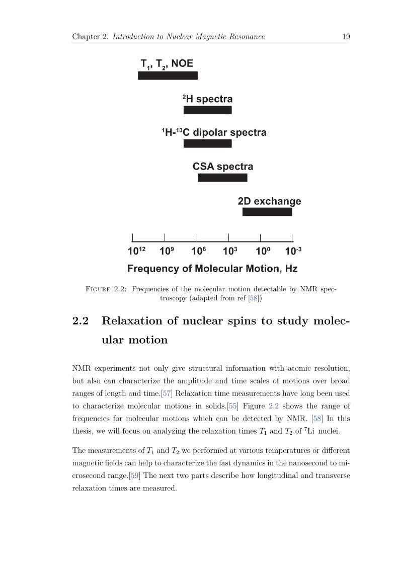
Frequency of Molecular Motion, Hz
103 1001061091012 10-3
T1, T
2, NOE
2H spectra
1H-13C dipolar spectra
CSA spectra
2D exchange
Figure 2.2: Frequencies of the molecular motion detectable by NMR spec-troscopy (adapted from ref [58])
2.2 Relaxation of nuclear spins to study molec-
ular motion
NMR experiments not only give structural information with atomic resolution,
but also can characterize the amplitude and time scales of motions over broad
ranges of length and time.[57] Relaxation time measurements have long been used
to characterize molecular motions in solids.[55] Figure 2.2 shows the range of
frequencies for molecular motions which can be detected by NMR. [58] In this
thesis, we will focus on analyzing the relaxation times T1 and T2 of 7Li nuclei.
The measurements of T1 and T2 we performed at various temperatures or different
magnetic fields can help to characterize the fast dynamics in the nanosecond to mi-
crosecond range.[59] The next two parts describe how longitudinal and transverse
relaxation times are measured.

Chapter 2. Introduction to Nuclear Magnetic Resonance 20
2.2.1 Longitudinal relaxation time T1
When one applies a RF (radio frequency) pulse on a spin system under a mag-
netic field, it will put the spin system into a thermodynamically unstable state.
The longitudinal relaxation time T1 is the characteristic time a spin system takes
to return to the equilibrium Boltzmann distribution of the populations. For a
mono-exponential relaxation behaviour, the evolution of magnetization after its
saturation by a train of RF pulses is given by:
Mz (t) = Mz (0)[
1 − exp(−t
T1
)]
(2.27)
where Mz (t) is the nuclear spin magnetization at time t, Mz (0) is the nuclear
spin magnetization at equilibrium. The pulse sequence used is a saturation re-
covery sequence, where the saturation pulse train (8 to 16 pulses, separated by
delays between 1 to 10 ms) is followed by a variable relaxation delay (t) and a π/2
"read" pulse which converts the relaxed magnetization into a detectable signal.
The relaxation rate is simply defined by R1 = 1/T1. For quadrupolar spins, a
consequence of their quadrupolar nature (as opposed to differences in the popula-
tions/environments) longitudinal relaxation is biexponential [60] and can be fitted
by using the equation:
Mz (t)
Mz (0)=
[
1 − 1
5exp
(
−t
T1,fast
)
− 4
5exp
(
−t
T1,slow
)]
(2.28)
However, if the difference between the two relaxation rates is small, usually, an
effective relaxation rates is measured and used in the calculations:
Mz (t)
Mz (0)=
[
1 − exp
(
−t
T1,eff
)]
(2.29)
2.2.2 Transverse relaxation time T2
After a perfect π/2 pulse, all spins are aligned in xy plane. The dephasing which
is caused by the sample’s inhomogeneity is prevented by the application of a
refocusing π pulse in the middle of the variable relaxation delay t (Hahn echo
sequence). The decay of the magnetization in the xy plan during the echo time
t is characterized by the transversal relaxation time T2. The equation describing

Chapter 2. Introduction to Nuclear Magnetic Resonance 21
mono-exponential transverse relaxation is:
Mxy (t) = Mxy (0) exp(−t
T2
)
(2.30)
For quadrupolar spins, the relaxation curve is also biexponential:[60]
Mxy (t)
Mxy (0)=
[
3
5exp
(
−t
T2,fast
)
+2
5exp
(
−t
T2,slow
)]
(2.31)
provided no residual quadrupolar interaction is present. As no splitting is ob-
served in our samples, we consider that no residual quadrupolar interaction is ever
observed in our samples. Similar to the case of longitudinal relaxation above, if
two transverse relaxation rates are close to each others, we have:
Mxy (t)
Mxy (0)= exp
(
−t
T2,eff
)
(2.32)
2.2.3 Molecular vibrations
The different types of motions which are relevant to the NMR experiments are
described in Levitt’s book.[52] We will briefly present about them. First, very fast
motions must be taken into account. This type of motion comes from the nuclei
which vibrates rapidly in their mean positions. The timescale of this motion
is in the range of 10−12 s (1012 Hz), thus it cannot be detected by relaxation
experiments (see figure 2.2) and the NMR Hamiltonians are effectively averaged
over this timescale.
2.2.4 Molecular flexibility
This motion comes from the internal flexibility (rotations around chemical bonds,
etc...) like in proteins or polymers. In our case, we studied PEO which is a
flexible polymer. The timescale of these motions can be short (picoseconds) to
much longer (seconds) when restraints to the motion are present.

Chapter 2. Introduction to Nuclear Magnetic Resonance 22
2.2.5 Molecular rotations
This type of motion comes from the rotationnal diffusion of molecules which can
be detected by modulations in the CSA, direct dipole-dipole or quadrupolar inter-
actions. In most case, the timescale lies in the range of picoseconds (10−12 s for
small molecules) to nanosecond (10−9 s for larger molecules) or 1012 to 109 Hz, so
that it can be detected by relaxation experiments.
It is very valuable to mention translational motion (the motion of the molecular
mass center through space) which is also detected by NMR. This type of motion
cannot be detected by relaxation experiments because its timescale is in microsec-
onds. To measure this motion, in this thesis, we used the method of pulse field
gradients (PFG) which is presented later.
2.3 How to study molecular motions with relax-
ation times
2.3.1 Angular dependent NMR interactions
As discussed above, the molecular motions can take place in a wide range of
timescale. The NMR interactions can detect the geometry and timescales of molec-
ular motions via isotropic and anisotropic nuclear spin interactions [57]. The re-
laxation processes characterized by T1, T2 are dominated by the NMR interactions
mentioned above. In other words, we understand the NMR interactions so we can
back-calculate the characteritics of molecular motions. In a recent paper, Hansen
et al. [57] have revisited the coupling between molecular motion and the NMR
interactions.
The general equation which describes the orientation-dependence of NMR inter-
actions can take the following form: [57, 61]
ω (θλ, φλ) − ωL = ωiso +∆λ
2
(
3 cos2 θλ − 1 − µλ sin2 θλ cos 2θλ
)
(2.33)
where ωL is Larmor frequency, ωiso is the isotropic frequency component. ∆λ, µλ
are asymmetry parameters, describing the deviation of axial system. The subscript

Chapter 2. Introduction to Nuclear Magnetic Resonance 23
λ describes the nature of the NMR interaction (CSA, dipole-dipole, quadrupolar
coupling). θλ, φλ denote the polar angles of the interaction PAS with respect to
external magnetic field.
Here, we should introduce an important concept: the order parameter. This pa-
rameter is the scaling factor of an interaction resulting from its averaging during
a given timescale. If the magnitude of the interaction does not fluctuate, during
this time, the tensor is distributed over an ensemble of thermally accessible orien-
tations defined by θ [62]. The order parameter S2 associated with this averaging
process can be written as:
S2 ≈ 1 − 3 〈θ2〉 (2.34)
2.3.2 Auto-correlation functions
If the Hamiltonian fluctuates, the solution to the Liouville-von Neumann will be
found by using a perturbation treatment as shown in equation 2.4: [63]
d ¯ρ
dt= −i
[
¯H, ¯ρ (0)
]
−∫ t
0
[
¯H (t) ,
[
¯H (t′) , ¯ρ (t′)
]]
dt′ (2.35)
where ρ0 is the thermal equilibrium of ρ.
Now, we will treat the Hamiltonian in form of spherical tensors which allows a
clear distinction between the time-dependent spin matrix elements and the time-
dependent spatial matrix elements. [64] The Hamiltonian in the laboratory frame
is given by:
H (t) =∑
α
Fα(t)Tα (2.36)
where Tα (α = k, l, λ) are the irreducible spherical tensor operators (acting on
the spin coordinates) of rank k and order l and λ denotes the type of interaction.
The ranks of irreducible spherical tensors Tα concern different interactions:
• Rank k=1: The spin-rotation and chemical shift anisotropy interactions
• Rank k=2: The dipolar and quadrupolar interactions

Chapter 2. Introduction to Nuclear Magnetic Resonance 24
Fα is the spatial part of the Hamiltonian interaction (linked to the orientation of
the interaction tensor in the laboratory frame): Fα (Ω (t)) = Fα (θ (t) , φ (t))
As equation 2.35 is developped, one can extract the spin parts from the integral,
and compute the integrals of products of the spatial parts Jα,α′ (ω):
Using this representation of the Hamiltonian, equation 2.35 will become:
d
dtρ (t) = −i
[
H0, ρ (t)]
(2.37)
−∑
α,α′
Jα,α′ (ω) [Tα, [Tα′ , (ρ (t) − ρ0)]]
The spectral densities Jα,α′ (ω) are the Fourier transforms of the correlation func-
tions, which express the correlation over time of the Fα functions with each other.
It can be written as: [53]
Gαα′ (|t − t′|) = 〈Fα (Ω (t)) Fα′ (Ω (t′))〉 (2.38)
where bra-ket notation is to show an ensemble or time average and (|t − t′|) = τ .
The Fourier transform of this correlation function transforms the time-dependent
Gαα′ (τ) function into a frequency-dependent function Jαα′ (ω):
Jαα′ (ω) =∫ ∞
0Gαα′ (τ) exp (iωτ) dτ (2.39)
which is called the spectra density.
For quadrupolar relaxation, the first order quadrupolar Hamiltonian is reduced to
only one term HQ = CQF2,0(t)T2,0, and cross-correlations with the much weaker
dipolar interactions will be neglected. Neglecting the effect of dipolar relaxation is
justified by the relative sizes of the interactions (tens of kHz for the quadrupolar
coupling, compared to 1.7 kHz for the dipolar interaction between 7Li and 1H if
they are 3 Å apart), and second we lack the necessary data to compute an extensive
model which would require many parameters. The only option would be to use
atomic trajectories from molecular dynamics simulations over sufficient timescales
to see if NMR relaxation parameters can be reproduced. Therefore, one has to
compute:
Gα (τ) =〈Fα (Ω (t)) Fα (Ω (t′))〉
〈F 2α (Ω (t))〉 (2.40)

Chapter 2. Introduction to Nuclear Magnetic Resonance 25
where 〈F 2α (Ω (t))〉 is the mean square of Fα (Ω (t)). Simple models of the corre-
lation functions usually consider it to be a mono-exponential decay with a time
constant τc. More generally, the correlation time τc expresses the time constant of
the decay of the reduced auto-correlation function, Gα (τ), which can be defined
as:
τα =∫ ∞
0Gα (t) dt (2.41)
Equation 2.39 can be written as:
Jα (ω) = 〈F 2α (Ω (t))〉 Jα (ω) (2.42)
where Jα (ω) is the reduced spectra density. We will focus on determining the
reduced spectra density from our relaxation data.
2.3.3 Determination of the spectral density
A nuclear spin relaxation rate R form can be written as:[64]
R (ωj, xi) = Aq (ωj, xi) (2.43)
where A represents the spin interactions.
The q (ωj, xi) function can be written as:
q (ωj, xi) =∑
j
njJ (ωj, xi) (2.44)
where ωj is a set of frequencies, xi is a set of parameters characterizing the dy-
namical processes involved.
From equation 2.42, equation 2.43 and equation 2.44 we can see the relationship
between relaxation rates, NMR interactions and molecular dynamics.
2.3.4 Spectral densities
Here, we present some spectral densities which are used frequently in fitting re-
laxation times.

Chapter 2. Introduction to Nuclear Magnetic Resonance 26
2.3.4.1 Bloembergen-Purcell-Pound (BPP) model
We started by analyzing the relaxation times T1 and T2 by the common Bloembergen-
Purcell-Pound (BPP) model [65–67], in which the correlation function is a single
exponential decay (i.e. one physical process, such as in the rotationnal diffusion
of a rigid molecule).
The spectral density is then given by:
Jn =τc
1 + n2ω2τ 2c
(2.45)
2.3.4.2 Cole-Davidson function
An other model was also tried, the so-called Cole-Davidson function:
Jn =2
ω
sin (β arctan (ωτc))[
1 + (n2ω2τ 2c )β/2
] (2.46)
where β(0 6 β 6 1) describes the deviation from exponentiality. This func-
tion originates from spectral density function used in dielectric relaxation.[68] The
Davidson-Cole spectral density is the most successful one used to interpret nuclear
spin relaxation experiments in solids.[64]
This function takes into account the distribution of motional barriers to correlated
motion like other models based on dielectric relaxation.
2.3.4.3 Lipari-Szabo model
This model-free approach is based on combining the effects of internal motion
-CI(t)- in molecules, which lead to partial averaging of the interactions, and of
the overall rotational motion -CO(t)- which averages the interactions over a longer
timescale.[69, 70]. For the case of isotropic overall motion, the total correlation
function is given by:
C (t) = CO (t) CI (t) (2.47)

Chapter 2. Introduction to Nuclear Magnetic Resonance 27
The internal correlation function is given by:
CI (t) = 〈P2 (µ (0) · µ (t))〉 = (1 − S2)e−t/τI + S2 (2.48)
where the unit vector µ describes the orientation of the interaction vector (or ten-
sor) in a reference frame and S2 describes the partial averaging of the interaction
by this internal correlation function. The overall correlation function CO (t) can
be defined in the case of isotropic or anisotropic motion, which is fully described
in reference. [70] In the case of isotropic molecules:
CO (t) = e−t/τO (2.49)
The spectral density is given by:
J (ω) =2
5
[
S2τO
1 + ω2τO
+(1 − S2) τe
1 + ω2τ 2e
]
(2.50)
where τO is the overall correlation time and τe is defined as:
1
τe
=1
τO
+1
τI
(2.51)
2.4 Diffusion
Diffusion is a phenomena, in which the molecules or small particles move randomly
due to the motion caused by thermal energy.[71] It is a transportation process of
particles in order to equalize the concentration in a whole system. The particles
will move from the high concentration places to low ones. Diffusion is a very
important process as it describes the mobility of each species (such as lithium
from one electrode to the other). This process can be presented by a specific
parameter D, called the diffusion coefficient with general unit in SI [m2/s]. Often,
D may follow an Arrhenius’ law:
D = D0 exp (−Ea/kBT ) (2.52)
whereas Ea is the activation energy, kB is Boltzmann’s constant , T is the absolute
temperature, D0 is the diffusion coefficient at infinite temperature.

Chapter 2. Introduction to Nuclear Magnetic Resonance 28
2.4.1 Fick’s laws
The Fick’s laws are used to describe the diffusion process. We will consider only
the one-dimension diffusion. The engine of the diffusion process is the concentra-
tion’s gradient. The movement of species is time and place-dependent; hence the
concentration is a function of the position and time t.
C = f (x, t) (2.53)
One can define the flux of diffusion J = ∂nS∂t
, where ∂n is the quantity of moving
species and S is the area perpendicular with the direction of diffusion. The first
Fick’s law describes the flux of one type of species(atoms, small particles etc...):
J =∂n
S∂t= −D
∂C
∂x= −DC (2.54)
where D is the diffusion coefficient(or the speed of diffusion when the gradient of
concentration is equal to unity). The sign ’-’ indicates that the flux J occurs in
the opposite direction of the concentration gradient (i.e. towards zones of lower
concentrations) and D is positive. The diffusion coefficient is expressed in [cm2/s]
or [m2/s].
ni(x) n
i(x+δ)
x-Axes
S1
Ji
dx
S2
Figure 2.3: Model of Fick’s laws

Chapter 2. Introduction to Nuclear Magnetic Resonance 29
The second Fick’s law is an expression of the law of conservation of matter:
∂C
∂t+ · J = 0 (2.55)
Combining with equation 2.54, we have:
∂C
∂t= · (DC) = D
∂2C
∂x2(2.56)
for a one-dimensional problem.
2.4.2 Self-Diffusion
2.4.2.1 Introduction
Self-diffusion is the transportation process without any chemical potential gradi-
ent, describing the uncorrelated movement of a particle. [72]
Figure. 2.3 explains how Fick’s laws are derived. The time it takes for the i species
to go from x to x + δ is τ (or the rate 1/τ). The probability for the i species to
go to the left or to the right are equal. The flux of i species that move across the
S plane is given by:
Ji = −[
n (x + δ, t)
τ− n (x, t)
τ
]
(2.57)
Since
C (x, t) =n (x + δ, t)
Sδ(2.58)
Therefore
C (x, t) − C (x + δ, t) = −δ∂C
∂x(2.59)
From equation 2.57 and equation 2.58, we have:
J = −δ2
τ
∂C
∂x(2.60)
Combining this with the first Fick’s law equation 2.54, we can derive the diffusion
coefficient in one-dimension:
D =δ2
τ(2.61)

Chapter 2. Introduction to Nuclear Magnetic Resonance 30
2.4.2.2 Stokes-Einstein equation
To explain Brownian motion, Einstein applied Stocks’ law to the diffusion of
species with Stokes drag ζ = 6πηR, and found the self-diffusion coefficient:
D =kBT
ζ(2.62)
This equation is also called Sunderland-Einstein equation.
2.4.2.3 Random walk theory
Now, we consider N species moving like in figure 2.3 with same velocity v =√
kBT/m, whereas kB is Boltzmann’s constant, m is the mass of the considered
species. The distance between the position of the species from their origins after
n jumps is:
〈x〉 =
∑
jx (j)
j(2.63)
Because the probabilities of jumps to the left and to the right are equal(half-half),
the average distance will be 〈x〉 = 0. To quantify the random walk movement,
we will focus on the mean square distance 〈x2〉, which is the characteristic of a
random walk:⟨
x2⟩
=
∑
j[x (j)]2
j(2.64)
The magnitude of 〈x2〉 is proportional to n jumps, and the time t:
⟨
x2⟩
∝ n,⟨
x2⟩
∝ t(2.65)
Now, we consider Figure. 2.3. The transit plane is in the middle between S1 and
S2, with the distance between each one is√
〈x2〉. The concentration of region
between S and S1 is C1, between S and S2 is C2. The diffusion flux of species
across the transit plane (or the net number of moles of species crossing through
the unit area of the transit plane per second from the left to the right) is given by:
J =1
2
√
〈x2〉t
(C1 − C2) (2.66)

Chapter 2. Introduction to Nuclear Magnetic Resonance 31
Since
C1 − C2 = −√
〈x2〉 dc
dx(2.67)
The equation 2.66 can be given:
J = −1
2
√
〈x2〉t
dc
dx(2.68)
In comparing with first Fick’s law equation 2.54:
D =
√
〈x2〉2t
or√
〈x2〉 = 2Dt (2.69)
Eq. 2.69 is also called the Einstein-Smoluchowski equation. It presents the micro-
scopic approach to diffusion. In two and three-dimensions, equation 2.69 trans-
forms into√
〈r2〉 = 4Dt and√
〈r2〉 = 6Dt, respectively.
2.4.2.4 Diffusion propagators
We consider the three-dimensional case with free isotropic diffusion, the propa-
gator is a function of the displacement but is independent of the initial position.
P (r0, r1, t) is the conditional probability of finding a particle initially in r0, and
in r1 after a time t. P (r0, r1, t) follows the normalization condition:
∫
P (r0, r1, t) dr1 = 1 (2.70)
The equilibrium particle density is given by:
ρ (r0) =∫
limt→∞
P (r0, r1, t) dr1 (2.71)
and∫
ρ (r0) dr0 = 1. The total probability P (r1, t) of finding a species at position
r1 at time t will be given by:
P (r1, t) =∫
ρ (r0) P (r0, r1, t) dr0 (2.72)
A detailed description can be found in.[73] Replacing C by P (r0, r1, t), the initial
condition can be written in the following form:
P (r0, r1, 0) = δ (r1 − r0) (2.73)

Chapter 2. Introduction to Nuclear Magnetic Resonance 32
where δ is the Dirac delta function. Then, equation 2.56 will become:
∂P (r0, r1, t)
∂t= D
2P (r0, r1, t) (2.74)
Eq. 2.74 has the following solution:
P (r0, r1, t) = (4πDt)−3/2 exp
[
−(r1 − r0)2
4Dt
]
(2.75)
2.4.3 Conductivity and diffusion
In this thesis, we focused on the materials used in battery systems. Therefore, the
connection between conductivity and diffusion is worth mentioning. The equations
were adapted from Modern Electrochemistry, vol 1. [74]
2.4.3.1 Mobility of Ions
Under an electric field, the random walk of ions becomes non-random. The ions
move in the direction dragged by the force þF with a drift velocity vd:
vd =dv
dtτ =
þF
mτ (2.76)
and τ is the time between ionic jumps. The absolute mobility is defined by:
uabs =τ
m=
vd
þF(2.77)
The absolute mobility uabs is the measure of drift velocity vd of ionic species under
force þF . The conventional (electrochemical) mobility is defined by:
uconv = uabszie0 (2.78)
whereas zie0 is the charge of ion.

Chapter 2. Introduction to Nuclear Magnetic Resonance 33
2.4.3.2 Nernst-Einstein equation
The molar ionic conductivity of a solution containing a z : z valent electrolyte is
given by:
Λ = F[
(uconv)+ + (uconv)−
]
(2.79)
where F is the Faraday constant. Combining Einstein relation D = uabskT with
equation 2.78, and replacing uconv, we have:
Λ =ze0F
kT(D+ + D−) (2.80)
This shows the direct relationship between conductivity and the sum of the self-
diffusion coefficients.
The ionic transport number (or transference number) is an important parame-
ter, describing the contribution of an ion to the overall conductivity. The ionic
transport number the cation t+ can be defined as:
t+ =u+
u+ + u−
=D+
D+ + D−
(2.81)
Hence, the transport numbers are related by: t− = 1−t+. In lithium batteries, the
cation transport number is of particular concern. A cation transport number of
one is expected to overcome the problems stemming from concentration gradients.
[75]
2.4.4 Diffusion coefficient measurements by NMR
In this thesis, we used the NMR method called "Pulsed Field Gradient" (PFG) to
measure the self-diffusion coefficients of spin bearing species. This is a noninvasive
method which is selective for nucleus of interest.[76]
A magnetic field gradient can be produced by a coil such as anti-Helmholtz or
Golay pairs of coils. When a magnetic field gradient G (T/m) is applied, where
the additional field is parallel to B0, it can be defined by: [77]
G = Bz =∂Bz
∂xi +
∂Bz
∂yj +
∂Bz
∂zk (2.82)

Chapter 2. Introduction to Nuclear Magnetic Resonance 34
where i, j ,k are unit vectors of the laboratory frame of reference. The precession
frequency of a nuclear spin will be modified:
ω (r) = ω0 + γ (G · r) (2.83)
We now consider the case of the magnetic field gradient is aligned with the z
direction, the magnitude of G will be: G = G · k = ∂Bz
∂z.
In the case of single quantum coherences, the cumulative phase shift experienced
by a nucleus in z(t) is given by:
φ (t) = γB0t + γ
t∫
0
G (t′) z (t′) dt′ (2.84)
the term γt∫
0G (t′) z (t′) dt′ is the result of the applied gradient. Eq. 2.84 shows the
dependence of the dephasing with the strength of the field gradient G(t) (pulsed
gradients have varying intensities), the duration t during which it is applied (oth-
erwise the field is homogeneous and no gradient is present), and the position z(t)
of the spin along the direction of the gradient.
The Hahn echo sequence [79] is used to measure diffusion coefficient by applying
the magnetic field gradient see Figure 2.4. The signal attenuation can be calculated
as:
S (2τ) = S (0) exp(
−2τ
T2
)
f (δ, G, ∆, D) (2.85)
The term of exp(
− 2τT2
)
expresses the attenuation due to relaxation. The function
f (δ, G, ∆, D) expresses the attenuation due to diffusion: as the diffusing species
are not in the same place after ∆, they do not experience the same gradient-induced
phase shifts, and therefore the magnetization is not refocused.
To eliminate the former term, we can perform several experiments with constant
∆ values and varying gradient strengths G. We then need to measure the following
quantity:
E =S (2τ)
S (2τ)g=0
= f (δ, G, ∆, D) (2.86)

Chapter 2. Introduction to Nuclear Magnetic Resonance 35
Figure 2.4: The Hahn spin-echo used to measure the diffusion coefficient. In(a), no diffusion means that the magnetizations of each slice in the sample alongz are refocused at the end. In (b), the random motion of spins implies that theydo not experience the same dephasing during the first and second gradient, and
therefore, the signal is incompletely refocused(adapted from ref [78])
The determination of the f function will lead to the diffusion coefficient D. Using
equation 2.75, for the standard spin-echo sequence, the expression of f is:
f (δ, G, ∆, D) = exp
[
−Dγ2g2δ2
(
∆ − δ
3
)]
(2.87)
In our case, the measurement of the diffusion coefficient was made with a gradient
applied along the MAS axis (see Figure 2.5), implying that MAS does not modulate
the gradient experienced by each spin. Such a gradient is created by applying three
gradients of equal strengths along the x, y and z axis. Diffusion is measured along
the MAS axis in this case.
In this thesis, we used the bipolar-gradient pulses which reduce the effects of
inhomogeneous background gradients and of eddy-currents.[81] As in our samples

Chapter 2. Introduction to Nuclear Magnetic Resonance 36
Figure 2.5: Magic Angle Spinning: rotating the sample around the diagonalof the cube exchange the x, y and z axis for each crystallite and thereforeaverages the anisotropic interactions. The three Euler angles α, β, γ describethe coordinate transformation from the MAS rotor frame to the laboratoryframe where β = θm (magic angle), γ = ωrt (ωr is the speed of rotation about
the rotor axis)(adapted from ref [80])
T Te
/2
rf pusle
gradient pusle
signal
/2 /2 /2 /2
Figure 2.6: Stimulated echo-bipolar gradient pulse sequence used to measurethe diffusion coefficient
T2 < T1, the magnetization was stored along z during ∆, as in the stimulated echo
sequence.
Figure 2.6 shows the pulse sequence that we used to measure the diffusion coeffi-
cient in this thesis. The f attenuation function is similar. To retrieve the diffusion
coefficient, several experiments are recorded, with varying gradient intensities,
keeping δ and ∆ constant. An example is shown below, in figure 2.7.
The measurements were performed on a 17.6 T wide-bore Advance HD Bruker
spectrometer, using a three axes Micro 2.5 G/A/cm gradient system coupled to
40 A amplifiers, therefore able to achieve a maximum 160 G/cm gradient with a 3.2

Chapter 2. Introduction to Nuclear Magnetic Resonance 37
0.8
0.6
0.4
0.2
0
1
0 20 40 60 80 100 120 140
Att
en
ua
tio
n o
f s
ign
al, S
/S0
Gradient strenght, G (G/cm)
T= 25 °C
D= 2.0 × 10⁻¹⁰ m2/s
= 4 ms
= 50 ms
Figure 2.7: Fitting the diffusion coefficient of Li+ in 1M LiPF6 in EC:DMC1:1.
mm Magic Angle Spinning (MAS), 1H -19F /31P-14N double resonance probe. To
ensure that experimental errors can be neglected, the measurements were repeated
several times and the presented results are averaged.


Chapter 3
The Effect of Magic Angle
Spinning on Relaxation and
Diffusion
3.1 Magic angle spinning
Magic angle spinning is a technique used to reduce inhomogeneous magnetic sus-
ceptibility effects [80] and anisotropic spin interactions such as CSA, dipolar cou-
pling and quadrupolar coupling (first order). This technique is usually used in
solid-state NMR. The spinning axis is inclined at the magic angle (54.74°) with
respect to the magnetic field B0, see figure 3.1.
Figure 3.1: Magic angle spinning of a rotor
39

Chapter 3. The Effect of Magic Angle Spinning 40
If the spinning frequency is high enough, the high-resolution isotropic NMR spec-
trum is obtained. Furthermore, small signals can become visible as narrower peaks
are easier to detect. [82] It should be mentioned that reducing the interactions
stated above can lead to an increase of T2 which limits the gradient pulse length
δ.
3.2 Temperature calibration
When the sample is rotated, friction forces tend to heat the rotor and the temper-
ature inside the rotor rises. Therefore, a proper monitoring of the temperature is
necessary. The temperature calibration for MAS spinning rates between 2 and 10
kHz with Pb(NO3)2. [83] To calculate the temperature inside the rotor, we used
the relationship between 207Pb chemical shift δCS and temperature: [83]
T () =δCS (ppm)
0.753 (ppm/)(3.1)
This equation works in the temperature range between -130 and +150 .
The temperature calibration under static conditions was done with ethylene glycol
(EG). [84] The relationship between the difference of the 1H chemical shifts of the
two peaks (∆δCS) and temperature is:
T (K) = 466.5 − 102.00 × ∆δ (ppm) (3.2)
This equation works in the temperature range between 273 and 416 K (or between
0 and +143 ).
3.3 Observation
The comparison of the 7Li spectra with different MAS rates is shown in figure 3.2.
The 7Li static spectrum can be fitted by two Lorentzian components (at the same
position), as expected from its quadrupolar nature. Table 3.1 shows the linewidth
of 7Li -NMR spectra in figure 3.2. Clearly, under MAS, the linewidth of the 7Li
spectrum becomes narrower than under static conditions. This shows that a clear
gain in sensitivity is obtained by MAS, allowing a significant gain in experimental

Chapter 3. The Effect of Magic Angle Spinning 41
07Li ref LiNO
3 (aq)
ppm
Static
kHz
10 kHz
Figure 3.2: 7Li NMR spectrum of PEO(LiTFSI) with different MAS rates at35 .
time, especially at lower temperatures, where the lines are broadened by residual
interactions. Interestingly, the linewidth is more or less the same under 2 kHz and
10 kHz MAS, as most residual interactions (quadrupolar, dipolar, susceptibility)
are quickly averaged by MAS.
Table 3.1: The linewidths (in Hz) extracted from the 7Li -NMR spectra ofPEO(LiTFSI) in figure 3.2
1st component 2nd component
Static 150.70 626.40
2 kHz 27.30 150.25
10 kHz 29.00 171.90
The experiments were performed also at higher temperatures up to 97 where
PEO(LiTFSI) is melted.
After our experiments at a 10 kHz MAS rate, we stored the sample in the glove
box. After one week, we ran a 1H -NMR spectrum, as seen in figure 3.3. The
lineshape of the 1H -NMR spectrum is clearly changed upon spinning, and the
splitting does not disappear quickly after spinning the sample. The same splitting
is also detected in the 7Li and 19F NMR spectra, as seen in figure 3.4, and the
lineshapes can be superimposed to each other if the scale is in ppm. Two questions

Chapter 3. The Effect of Magic Angle Spinning 42
10 8 6 0 10 8 6 0 ppm1H ref TMS
After 10 kHz-MAS
Figure 3.3: Comparison of the static 1H -NMR spectra of PEO(LiTFSI) before(left) and after (right) the experiments 10 kHz-MAS. These experiments were
performed at 31
F ref 4’-fluoroacetophenone
ppm
7Li ref LiNO3 (aq)
Figure 3.4: Static 7Li - and 19F -NMR spectra of PEO(LiTFSI) at room tem-perature after spinning the samples at a 10 kHz MAS rate.
arise: what happens to the polymer sample? How does this affect other properties
such as diffusion and relaxation?
3.4 Previous studies
Kawamura et al. explain in their paper [85] that spinning the sample generates
a pressure on it, because of the centrifugal forces that press the sample against
the inner wall of the rotor. Calculations show that MAS induce a pressure that
is proportional to the square of the MAS frequency. They observed the pressure
effect on the equilibrium constant of [all-trans-bR]/[13-cis-bR] in retinal. They

Chapter 3. The Effect of Magic Angle Spinning 43
10 8 6 0
1H ref TMS
10 8 6 0 ppm
97 °C
10 kHz
1 hour
Static
Figure 3.5: Comparison of 1H -NMR spectrum under 10 kHz MAS at 97
(left) and under static condition at 25 (right)
also observed how this pressure generates isomerization of retinal from all-trans
to 13-cis state in the membrane protein bR.
Asano et al. [86] studied by 1H MAS-NMR styrene-butadiene rubbers samples
(SBR) filled with SiO2 (SBR/Si composite). They realized that the molecular
motion of SBR/Si composites became slower because of the centrifugal forces
caused by spinning the sample. The authors have also calculated the pressure
P (Pa) generated by MAS at νR (Hz), the inner radius of the rotor r(m) and the
sample density ρ (kg/m3) by: [85, 87]
P =4
3π2ν2
Rr2ρ (3.3)
Furthermore, MAS affects also longitudinal relaxation T1 of 1H . It is shown that
the molecular motions are affected by the centrifugal force.
Kitamura et al. [3] observed also the effects of pressure when studying 13C MAS-
NMR spectrum of natural rubber(NR). The 13C -NMR spectrum, after MAS at
9 kHz for 1 days at 333 K, showed anisotropic peaks. The elongated sample
showed a doublet-like peak. However, WAXD analysis exhibited that there was no
crystalline phase presents, so that the doublet-like peak is caused by the existence
of some molecular orientation.
Kitamura [3] showed that this lineshape did no arise from a crystalline phase
but was caused by the existence of molecular orientation, which affects the local
magnetic susceptibility tensor (explaining why the lineshape is the same for all
nuclei when compared in ppm).
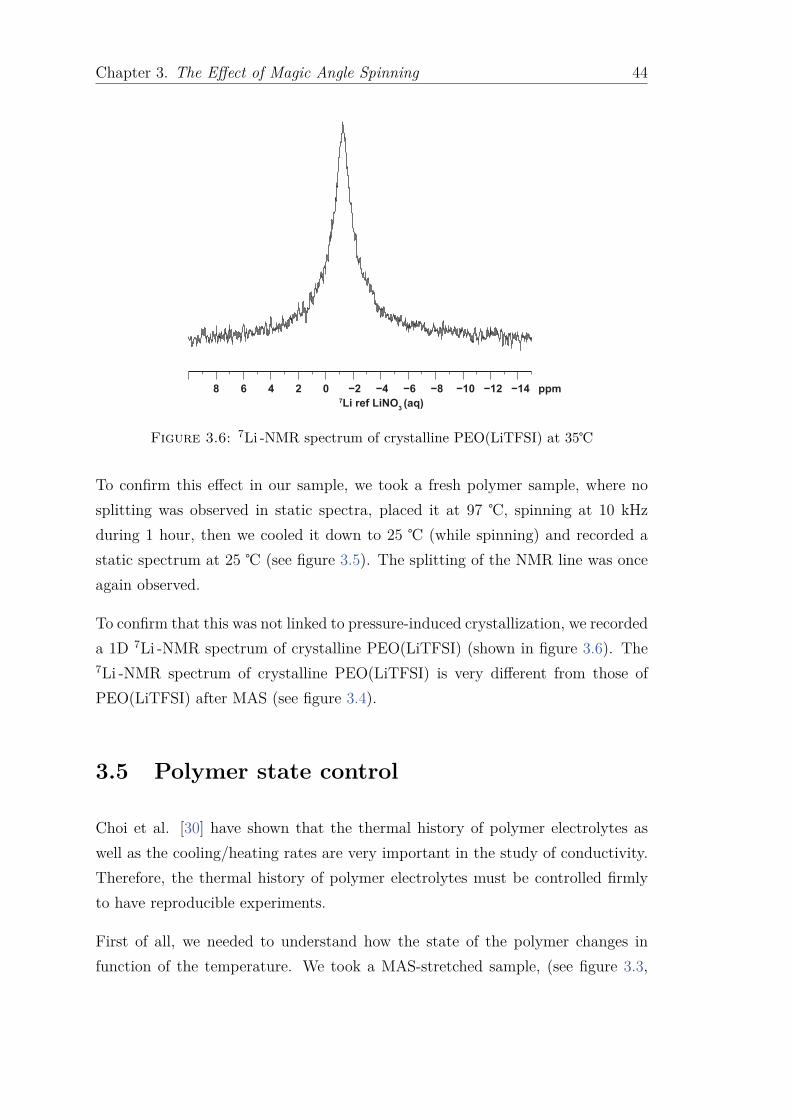
Chapter 3. The Effect of Magic Angle Spinning 44
ppm7Li ref LiNO
3 (aq)
Figure 3.6: 7Li -NMR spectrum of crystalline PEO(LiTFSI) at 35
To confirm this effect in our sample, we took a fresh polymer sample, where no
splitting was observed in static spectra, placed it at 97 , spinning at 10 kHz
during 1 hour, then we cooled it down to 25 (while spinning) and recorded a
static spectrum at 25 (see figure 3.5). The splitting of the NMR line was once
again observed.
To confirm that this was not linked to pressure-induced crystallization, we recorded
a 1D 7Li -NMR spectrum of crystalline PEO(LiTFSI) (shown in figure 3.6). The7Li -NMR spectrum of crystalline PEO(LiTFSI) is very different from those of
PEO(LiTFSI) after MAS (see figure 3.4).
3.5 Polymer state control
Choi et al. [30] have shown that the thermal history of polymer electrolytes as
well as the cooling/heating rates are very important in the study of conductivity.
Therefore, the thermal history of polymer electrolytes must be controlled firmly
to have reproducible experiments.
First of all, we needed to understand how the state of the polymer changes in
function of the temperature. We took a MAS-stretched sample, (see figure 3.3,

Chapter 3. The Effect of Magic Angle Spinning 45
10 8 6 0 ppm
Temperatu
re, T (°C
) 31
55
67
79
91
1H ref TMS
Figure 3.7: The evolution of the static 1H -NMR Hahn echo spectrum as afunction of temperature
right hand side), we recorded 1H -NMR 1D spectra at various temperatures, in-
terleaving 30 minutes waiting times between each temperature point. Figure 3.7
shows the evolution of the 1D 1H NMR Hahn echo spectrum. From 31 to 55 the
splitting survives, and starts vanishing at 67 , when the polymer starts melting.
Kitamura [3] have observed same disappearance of the splitting when the sample
is annealed.
The presence of a narrow component (disordered polymer) and of a splitting (still
ordered polymer) may come from residual temperature gradients (the polymer
is not melted everywhere in the sample), and from the kinetics of the polymer
chain reorientation. To check the kinetics of this phenomenon, we recorded a se-
ries of 1H NMR spectra at 97 after various evolution times (see Figure 3.8). No
evolution is detected after 40 minutes, and the polymer can be considered as disor-
dered at that stage (the lineshape is still affected by shimming and inhomogeneity
issues).
We dropped the temperature down from 97 to 25 within 1 minute, as seen in
figure 3.10 to freeze the polymer in the disordered and amorphous state. 1H NMR
spectra were recorded at 25 as a function of time (Figure 3.9). No evolution
whatsoever of the 1H NMR spectrum was detected after one hour.

Chapter 3. The Effect of Magic Angle Spinning 46
10 8 6 0 ppm
Tim
e, t (min
)
0
10
30
50
1H ref TMS
60
Figure 3.8: The evolution of the static 1H -NMR Hahn echo spectrum at 97 as a function of time
10 8 6 0 ppm
Tim
e, t (h)
0
1
3
1H ref TMS
Figure 3.9: The evolution of the 1H -NMR spectrum at 25 after quenchingthe sample from 97 under static condition

Chapter 3. The Effect of Magic Angle Spinning 47
Polymer sample 97 °C
10 KHz-MAS
Static
1 hour
25 °C, Static1 min
Amorphous Polymer
Ordered Polymer
Figure 3.10: The scheme for controlling the polymer state
To ensure the reproducibility of our experiments, we introduced the following tem-
perature treatment scheme (figure 3.10). The polymer sample is first completely
melted at 97 , and quenched at 25 by shutting down the heating system. Af-
ter one hour, the sample is considered as stabilized, and the temperature is raised
at the desired temperature for relaxation or diffusion experiments. It turns out
that such procedure may damage the NMR probehead and lead to difficulties in
spinning the sample after a couple of heating/cooling cycles.
3.6 Diffusion and relaxation time results
It is very interesting to compare the results of diffusion and relaxation experiments
with and without MAS. At the start, the sample was always conditioned in the
amorphous state. Equation 3.3 was used to calculate the inner pressure induced
by MAS with νR = 104 Hz, r = 1 × 10⁻³ m, ǫ = 1.13 × 10³ kg/m3. Therefore, the
inner pressure inside a 3.2 mm rotor under 10 kHz MAS is around P = 15 bar.
Figure 3.11 shows the comparison of diffusion coefficients of Li+ and TFSI− under
10 kHz MAS and in static conditions, at the same temperature (taking into account
the real temperature inside the rotor). At around 60 , the change in the slope
occurs at the melting temperature of our PEO(LiTFSI) polymer sample. The
diffusion coefficients are fitted with an Arrhenius law, the activation energies can
be found in table 3.2.
Table 3.2: Activation energies calculated (in kJ/mol) for DLi+ and DTFSI−
using an Arrhenius law.
Static 10 kHz-MAS
Li+ TFSI− Li+ TFSI−
Below TM 101.25 ± 1.69 107.39 ± 3.42 127.90 ± 20.90 126.94 ± 16.61
Above TM 38.15 ± 0.80 37.62 ± 0.84 47.72 ± 1.57 43.55 ± 1.71

Chapter 3. The Effect of Magic Angle Spinning 48
100 80 60 40 20
2.6 2.8 3 3.2 3.4
10-13
10-12
10-11
10-10
1013
1012
1011
1010
Temperature, T (°C)
1000/T (K-1)
Dif
fus
ion
Co
eff
icie
nt,
D (
m2/s
) T
M
59.6°C
Figure 3.11: Diffusion coefficients of Li+( ) and TFSI−(N) under 10 kHzMAS (open blue symbols) and in static conditions (full green symbols). Thecontinuous lines are Arrhenius fits. At low temperatures, the sensitivity of MAS
experiments is much better than their static counterparts.
The diffusion coefficients can also be fitted with a VTF equation, as seen in figure
3.12. The table 3.3 shows the pseudo-activation energies calculated by the VTF
fit.
Table 3.3: Pseudo-activation energies (kJ/mol) calculated for DLi+ andDTFSI− using a VTF law, with T0 = −40 .
Static 10 kHz-MAS
Li+ TFSI− Li+ TFSI−
Below TM 7.34 ±0.19 7.77 ±0.36 9.82 ±1.39 9.72 ±1.06
Above TM 4.58 ±0.13 4.50 ±0.20 5.46 ±0.14 5.01 ±0.13
In figure 3.11, the diffusion coefficients of species look very similar under both
conditions. The activation energies are 18-25 % higher under MAS than in the
static sample. However, when taking into account the error of the fits, we saw
that the activation energies get close to each others . Anisotropic diffusion was

Chapter 3. The Effect of Magic Angle Spinning 49
100 80 60 40 20
2.6 2.8 3 3.2 3.4
10-13
10-12
10-11
10-10
1013
1012
1011
1010
Temperature, T (°C)
1000/T (K-1)
Dif
fus
ion
Co
eff
icie
nt,
D (
m2/s
)
TM
59.6°C
Figure 3.12: Diffusion coefficients of Li+( ) and TFSI−(N) under 10 kHzMAS (open blue symbols) and in static conditions (full green symbols). The
continuous lines are VTF fits.
not detected as no deviation from the Gaussian decay was observed in the fitting
of the attenuation curve.
On the one hand, we know that MAS has modified our sample, and that the
pressure has induced some kind of alignment of the polymer chains. On the other
hand, the diffusion coefficient does not change significantly under MAS, and no
significant anisotropy is detected, as opposed to what Golodnitsky et al. [88] have
found for PEO9LiI: the diffusion coefficient of Li+ measured at 60 can be 1.4
times faster (‖ the stretched direction), 2.7 times slower (⊥ the stretched direction)
than in the unstretched one.
The longitudinal relaxation time T1 were also recorded, as seen in figure 3.13. Inter-
estingly, the longitudinal relaxation seems to be unaffected by spinning, although
at higher temperatures, a slight difference can be detected. This may indicate
that the dynamics at the nanosecond level (or close to the Larmor frequency) are
unaffected by pressure.

Chapter 3. The Effect of Magic Angle Spinning 50
100 80 60 40 20Temperature, T (°C)
2.6 2.8 3 3.2 3.40.8
1.2
1.6
2
7L
i N
MR
Rela
xati
on
Rate
(s
-1)
1000/T (K-1)
Figure 3.13: The longitudinal relaxation times T1 of Li+ in PEO(LiTFSI)under 10 kHz MAS (open blue symbols), 2 kHz MAS (open red symbols) and
in static conditions (full green symbols)
3.7 Conclusion
The effect of MAS on PEO(LiTFSI) have been explored by 1D-NMR, PFG diffu-
sion and relaxation rates measurements. The presence of a slitting is clearly caused
by the change in the magnetic susceptibility tensor which is induced by MAS. This
change occurs upon the ordering of the polymer chains under the pressure which
results from the centrifugal forces. The diffusion coefficients of the electrolyte
species and their mobility at the nanosecond timescales seem unaffected. The ac-
tivation energy of the diffusion coefficients seem to be similar upon spinning the
sample when we took into account the error of the fits.
The splitting is removed by melting the polymer sample, and therefore we imple-
mented a systematic heating/cooling cycle to trap the polymer in the amorphous
state and ensure the reproducibility of our experiments.
In the following, our study on relaxation rates and diffusion coefficients was per-
formed on static samples, in order to avoid potential effects induced by MAS, such
as on polymer’s morphology.

Chapter 4
Relaxation times and diffusion
coefficient measurement
4.1 Introduction
Lithium-polymer batteries display high specific capacities and high voltages as
they benefit from the lithium-metal anode. However, at high charging rates,
lithium dendrites tend to appear and lead to short-circuits, battery fire and ex-
plosions as the mechanical strength of the classical PEO polymer is small. One
way to overcome this limit is to use nano-structured block copolymers[1], in which
PS blocks provide the missing mechanical strength. Above their melting tem-
peratures, block-copolymers display lower conductivities than pure PEO, as the
tortuosity of the phase separated polymer slows the diffusion of Li+ down. [50]
However, at lower temperatures, the confinement effect reduces the melting tem-
perature of the PEO domains, and the ionic conductivity of block-copolymers is
comparable to the conductivity of neat PEO.
The mechanisms of Li+-motion were well discussed in many papers.[89] It is as-
sumed that the Li+ cation diffusion process is governed by the coupling of the
mobile Li+ cation with the structural relaxation modes of the polymer chains, and
many studies are focused on the characterization of the polymer chain motion.
For ion concentrations that give the maximum conductivity, single lithium ions
are expected to be coordinated by 5-6 ether oxygens [90] and the local structures
observed in crystals are expected to survive above the melting temperature. [91]
51

Chapter 4. Relaxation times and diffusion coefficient measurement 52
Several models[92–94] describe three mechanisms of Li+-motion, corresponding to
motion along the polymer chain, correlated motion with the chain segments, and
jumps between neighboring chains. Molecular dynamics show that lithium ions
can complex oxygen atoms from several PEO chains and therefore act as cross-
links with a lifetime of 13 to 40 ns [92, 95] and motions occur through changes
in the lithium-oxygen bond network, with Li+- EO bonds that have a 0.1 to 1 ns
lifetime.[96] All in all, theoretical studies based on analytical models or molecular
dynamics calculations are usually in good agreement with self-diffusion coefficient
or conductivity measurements. Quasi-elastic neutron scattering is usually lim-
ited to timescales around 0.1 ns, while neutron spin-echo spectrometry was used
to comprehend polymer dynamics at timescales below 1.7 ns.[97] Nuclear Mag-
netic Resonance spectroscopy, on the other hand, can study 7Li motion above the
nanosecond timescale, but most studies obtained a single characteristic time and
fail to describe the motional process in a more detailed manner. A recent study
[98] highlights that contrary to the widespread belief that polymer chain motions
control the ionic diffusion, the ionic mobility can be decoupled from chain motions.
Therefore, more information is needed to directly characterize the motion of Li+
at the nanosecond-nanometer scale in order to design polymer electrolytes with
better mechanical properties and conductivities.
On the one hand, pulse-field gradients NMR (PFG-NMR) can be used to mea-
sure self-diffusion coefficients, which are measured for Li+ displacement over 1-2
µm. On the other hand, Nuclear Magnetic Resonance (NMR) relaxation is able
to characterize the dynamics of the fluctuations of the Hamiltonians that govern
the spin system evolution. For 7Li (S = 3/2), the relaxation of the spin system
is governed by the quadrupolar interaction, which results from the presence of an
electric field gradient (EFG) at the nucleus and are created by asymmetric charge
distribution in the lithium environment. Longitudinal relaxation (characterized
by T1), for example, describes how the lithium spin polarization builds up and
is the most efficient when the characteristic frequencies of the fluctuations of the
quadrupolar interaction are close to the 7Li Larmor frequency. Transverse relax-
ation (T2), which describes the non-refocusable decay of single-quantum coherences
is affected by slow and fast fluctuations alike, and when slow fluctuations domi-
nate, a bi-exponential magnetization decay is observed. Most of the 7Li relaxation
measurements were made so far at a single high magnetic field and usually pro-
vided a single correlation time τc for the fluctuation of the lithium ion quadrupolar

Chapter 4. Relaxation times and diffusion coefficient measurement 53
interactions in the nanosecond regime. Relaxometry, on the other hand, is per-
formed at lower magnetic fields (lower than 1 T) and has been mostly used to
characterize motions on a frequency range from kHz to 10s of MHz for 1H or 19F ,
and therefore does not probe motion at the nanosecond timescale for 7Li .
In this thesis, we measured longitudinal and transverse 7Li relaxation rates at
three magnetic fields (4.7, 9.4 and 17.6 T) and various temperatures ranging be-
tween 25 and 100 . The usage of relaxometry at high fields helps us to detect the
range of motion from ns to 10s of ns. The longitudinal relaxation was observed
to be single-exponential while, for transverse relaxation, bi-exponential relaxation
was observed below the melting temperature for PEO(LiTFSI) and at all tem-
peratures for PS-PEO(LiTFSI)-PS. Interestingly, above melting temperature, in
PEO(LiTFSI), the transverse relaxation time was observed as single-exponential.
These relaxation rates were fitted using the Maple software with the simplest
model possible describing 7Li quadrupolar relaxation with a perturbation stem-
ming from heteronuclear dipolar relaxation and featuring four adjustable param-
eters, including two nanosecond timescales τ1 and τ2. Simpler models, all de-
rived from Bloembergen-Purcell-Pound (BPP) theory,[65, 99] failed to correctly
reproduce the observed relaxation rates. Similarly, using stretched exponentials
or Cole-Davidson functions for correlation functions [100–102] failed to produce
satisfying results.
4.2 Diffusion coefficient and conductivity of poly-
mer samples
The diffusion coefficients of polymer samples were measured under static condition
by PFG-NMR, as seen in figure 4.1. The melting temperature TM of PEO(LiTFSI)
and PS-PEO(LiTFSI)-PS was estimated by the change of slope in the diffusion
coefficient curve, and the melting temperature was calculated with the averaged
temperatures measured before and after such the discontinuity. The melting tem-
perature, here, is expected to be the melting temperature of the PEO part.
Measurements were conducted such that the mean free path the ions diffusively
explored over the diffusion time ∆ was approximately 2 µm. The equation is used

Chapter 4. Relaxation times and diffusion coefficient measurement 54
100 80 60 40 20
2.6 2.8 3 3.2 3.4
10-13
10-12
10-11
10-10
1013
1012
1011
1010
Temperature, T (°C)
1000/T (K-1)
Dif
fus
ion
Co
eff
icie
nt,
D (
m2/s
) TM
TM
59.6°C
55.5°C
Figure 4.1: Diffusion coefficients of PEO(LiTFSI) and PS-PEO(LiTFSI)-PSmeasured under static condition: Li+( ), TFSI−(N). The lines are guides forthe eyes, and the activation energies were calculated for diffusion coefficientusing an Arrhenius law. The melting temperature of PEO(LiTFSI) and PS-
PEO(LiTFSI)-PS were estimated around 59.6 and 55.5 , respectively.
to calculate the mean free path:
I =√
6D∆ (4.1)
Interestingly, the anion TFSI− is more mobile than the Li+ cation regardless of
their respective sizes. The same phenomenon was also observed in previous studies.
[2, 103, 104] It was explained by the interaction Li+... O between lithium ions and
oxygens in polymer chains.
The difference of TM between PEO(LiTFSI) and PS-PEO(LiTFSI)-PS may come
from the difference in molecular weight of the PEO part which is 100000 g/mol
for PEO(LiTFSI) and 35000 g/mol in PS-PEO(LiTFSI)-PS. Furthermore, the
decrease of the melting temperature may come from the confinement effect [105,
106] which also reduce the PEO domains crystallinity below TM.

Chapter 4. Relaxation times and diffusion coefficient measurement 55
Above TM, both of Li+ and TFSI− in PEO(LiTFSI) have higher diffusion coeffi-
cients than those in PS-PEO(LiTFSI)-PS. It is due to the PS domain which has
a melting temperature of up to 240 . [107] The presence of PS domains over a
length scale of nanometers (into which Li+ and TFSI− cannot diffuse) slows down
the overall diffusion. The diffusion activation energies of Li+ and TFSI− are very
similar for both polymer samples.
Below TM, both of Li+ and TFSI− in PS-PEO(LiTFSI)-PS diffuses faster than
those in PEO(LiTFSI). This interesting results can be explained by the confine-
ment effect [105, 106], which lowers TM in PS-PEO(LiTFSI)-PS and decrease its
crystallinity. More amorphous region, with more mobility for polymer chains (τ2
is shorter in PS-PEO(LiTFSI)-PS, see section 4.3) will give rise to higher diffusion
coefficients, even though tortuosity slows diffusion down. The activation energies
of Li+ and TFSI− are nearly similar for PEO(LiTFSI). For PS-PEO(LiTFSI)-PS,
one can find that the activation energies of Li+ is significantly smaller than the
one measured for TFSI−. Table 4.1 shows the activation energies calculated by
the Arrhenius law for the self-diffusion coefficients of Li+ and TFSI−.
Table 4.1: Activation energies calculated (kJ/mol) for DLi+ , DTFSI− and forthe ionic conductivities, measured experimentally and computed from the dif-
fusion coefficients, both using an Arrhenius law.
PEO(LiTFSI) PS-PEO(LiTFSI)-PS
Diffusioncoefficient
Li+ TFSI− Li+ TFSI−
Below TM101.25±1.69
107.39±3.41
68.86±6.24
87.84±5.14
Above TM38.15±0.80
37.62±0.84
40.80±0.63
39.64±0.94
Ionic conductivity
(experimental /
Nernst-Einstein
equation)
PEO(LiTFSI) PS-PEO(LiTFSI)-PS
Below TM 144.08 ±25.21/103.35 ±2.86 97.89 ±14.01/92.18 ±4.46
Above TM 27.95 ±0.31/34.79 ±0.67 37.37 ±1.05/36.95 ±0.86
The conductivities of PEO(LiTFSI) and PS-PEO(LiTFSI)-PS were also measured,
as seen in figure 4.2. Activation energies of the conductivity were calculated with

Chapter 4. Relaxation times and diffusion coefficient measurement 56
100 80 60 40 20
2.6 2.8 3 3.2 3.410
10
10
10
106
10
104
103
Ion
ic c
on
du
cti
vit
y,
(S
/cm
)
Temperature, T (°C)
1000/T (K-1)
TM
TM
42°C
Figure 4.2: Ionic conductivities of PEO(LiTFSI) and PS-PEO(LiTFSI)-PS.The full symbol indicates experimental data while the open symbol indicatesthe data calculated with the Nernst-Einstein equation. The lines are guides forthe eyes, and the activation energies were calculated for diffusion coefficientsusing an Arrhenius law. The melting temperature of PEO(LiTFSI) and PS-
PEO(LiTFSI)-PS were estimated around 52 and 42 , respectively.
an Arrhenius law and the values can be found in table 4.1. The TM found by
conductivity and diffusion differ. This difference can be assigned to the kinetic of
crystallization process. For diffusion measurements, we increased the temperature
and waited until the system to be equilibrated. For conductivity measurements,
the inverse process was performed by decreasing in the temperature. Therefore,
the percent of PEO crystalline in both cases may be different to each others and it
leads to the difference in melting temperature. However, the agreement between
the curve is relatively good.
As expected, above TM, the ionic conductivity in PEO(LiTFSI) is higher than
in PS-PEO(LiTFSI)-PS. Below TM, the inverse phenomena is observed again.
However, the activation energies calculated from conductivity and diffusion mea-
surements are different.

Chapter 4. Relaxation times and diffusion coefficient measurement 57
Tra
ns
fere
nc
e n
um
be
r
0.2
0.4
0.6
0.8
0.19±0.01
0.22±0.01
100 80 60 40 20
2.6 2.8 3 3.2 3.4
Temperature, T (°C)
1000/T (K-1)
1.0
0
Figure 4.3: The transference numbers of Li+( ) and TFSI−(N) inPEO(LiTFSI) and PS-PEO(LiTFSI)-PS. The dashed lines show the average
values of transference numbers.
The conductivity calculated by the Nernst-Einstein equation shows an overesti-
mated value in comparing with experimental data, see figure 4.2, the same obser-
vation was reported by Arumugam. [2] The main reason may be the presence of
ion pairs and of larger ion clusters which do not (or less) contribute to the con-
ductance. The existence of ion pairs may be expected as the diffusion activation
energies for Li+ and TFSI− are similar, seemingly indicating a correlated diffusion
process.
Figure 4.3 show the transference number of Li+ and TFSI− in PEO(LiTFSI) and
PS-PEO(LiTFSI)-PS, the calculation was performed by using the equations:
t+ =DLi+
DLi+ + DTFSI−
(4.2a)
t− =DTFSI−
DLi+ + DTFSI−
(4.2b)
The transference numbers seem to be temperature-independent. The average

Chapter 4. Relaxation times and diffusion coefficient measurement 58
100 90 80 70 60
2.6 2.7 2.8 2.9 30.5
1.0
1.5
2.0
To
rtu
os
ity
Temperature, T (°C)
1000/T (K-1)
Figure 4.4: The tortuosities of Li+( ), TFSI−(N) in PS-PEO(LiTFSI)-PSwere calculated by using equation 4.3; Li+( ), TFSI−(N) present for the tor-tuosities calculated by taking into account of volume fraction of PEO-TFSI(ǫ=0.707). The tortuosity from conductivity is calculated by equation 4.4 ().
The dashed lines represent for average values of each species.
transference numbers of Li+ are 0.22 ±0.01 and 0.19 ±0.01 for PEO(LiTFSI)
and PS-PEO(LiTFSI)-PS, respectively.
In PS-PEO(LiTFSI)-PS, the diffusion of species is deviated from straight path by
the presence of PS domains (see figure 4.5a). [108] The tortuosity (T ) represents
this deviation and was calculated by: [108]
T =Dm
Dm′
(4.3)
where Dm, Dm′ are the diffusion coefficients of diffusing species without and with
the presence of PS part, respectively. The equation 4.3 will be T =DPEO(LiTFSI)
DPS-PEO(LiTFSI)-PS.
Figure 4.4 shows the tortuosity calculated for PS-PEO(LiTFSI)-PS, assuming
that, on the lengthscale of PEO domains, the diffusion coefficients are equal
whether they are attached to PS chains at each end or not.
The calculation was performed above the melting temperature, as below TM, crys-
talline domains may be found in PEO (in which Li+ can’t diffuse), creating some
sort of undetermined tortuosity. As presented in ref. [50], Bouchet et al. have
discussed the effect of the PS part in PS-PEO(LiTFSI)-PS. They proposed that

Chapter 4. Relaxation times and diffusion coefficient measurement 59
RPEO
D0
l
x
a. b.
Figure 4.5: (a) Representation of tortuosity: the red arrow presentsthe straight path of the moving species in case of homogeneous polymerPEO(LiTFSI) while the blue one presents for the case of block copolymerPS-PEO(LiTFSI)-PS. The black areas shows for the PS domains. (figureadapted from ref [108]) (b) Size of polymer domains in block copolymer PS-
PEO(LiTFSI)-PS where RP EO=9.45 nm, D0=25 nm.
the tortuosity can be calculated by:
T (ǫ) =σ0ǫ
σ(4.4)
where ǫ is the volume fraction of PEO-LiTFSI. σ0 and σ are the conductivities
of pure PEO(LiTFSI) and PS-PEO(LiTFSI)-PS, respectively. The authors pos-
tulated the existence of a "dead-zone" where ionic motion is forbidden (see figure
4.6). [106] The volume fraction of PEO domains seemed to be smaller than ex-
pected, indicating that a fraction of the PEO volume, at the interface between PS
and PEO, is either forbidden for Li+ or its conductivity is considerably reduced
in it. The conductivity is affected by the volume fraction of PEO-LiTFSI and
the thickness λ of the dead zone at the PS/PEO interface. The tortuosity was
recalculated:
T (ǫ) =σ0ǫ (λ)
σ (ǫ)(4.5)
The tortuosity calculated from diffusion coefficients with taking into account the
volume fraction of PEO is, interestingly, close to what was obtained from the
conductivities.
However, the assumption that the conductivity in PEO domain of PS-PEO(LiTFSI)-
PS is identical to the conductivity in homogeneous PEO(LiTFSI), need to be
proved. The technique PFG-NMR as well as conductivity measure ionic displace-
ments at the macroscopic length scale (i.e. ≥ 1 µm). Therefore, to understand

Chapter 4. Relaxation times and diffusion coefficient measurement 60
Dead zone
PEO domain PS domainPS domain
Li+TFSI-
Figure 4.6: The representation of the microstructure of the BCE. The hatchedred areas show the "dead zone" where the ions can’t diffuse. The purpose areas
are PEO crystallites. (figure adapted from [50])
the Li+ mobilities over the size of the PEO domains (≈ 20nm, see figure 4.5b), we
need relaxation study.
4.3 Relaxation rates R1 and R2 characterization
4.3.1 Calculation of relaxation rates
The relaxation matrix, R can be described as:[109]
R = RQ + RD + R
CSA (4.6)
assuming that the fluctuations of the quadrupolar (Q), dipolar (D) and chemical
shift anisotropy interactions (CSA) are not correlated. For 7Li (S = 3/2), the
relaxation of the spin system is governed by the quadrupolar interaction, which
results from the presence of an electric field gradient (EFG) at the nucleus, created
by asymmetric charge distribution in the lithium environment. The relaxation rate
of quadrupolar nuclei have been calculated elsewhere and are linear combinations
of the spectral density function JQQ(0), JQQ(ω0) and JQQ(2ω0) which are the
Fourier transforms of the correlation function CQQ(τ) at 0, once and twice ω0 (the
Larmor frequency). [60]
For longitudinal relaxation time (T1), the bi-exponential curve was showed as 80/20
% weight for the fast and slow components. However, these two rates are very

Chapter 4. Relaxation times and diffusion coefficient measurement 61
0
0.2
0.4
0.6
0.8
1.0
0 108642
Mz(t
)/M
z(0
)
t (s)
0
0.2
0.4
0.6
0.8
1.0
0 108642t (s)
a. b.
Mz(t
)/M
z(0
)
Figure 4.7: Comparison of bi-exponential (a) and single-exponential (b) lon-gitudinal relaxation fits (7Li longitudinal relaxation time of PEO(LiTFSI) at 35
). There is almost no difference between bi- and single-exponential fits.
close to each others and a single-exponential magnetization recovery was detected
with an effective longitudinal relaxation rate (see figure 4.7 and section 2.2.1 for
details) equal to:
R1 =4π2
⟨
C2Q
⟩
50[J (ω0) + 4J (2ω0)] (4.7)
For transverse relaxation, the behavior is clearly bi-exponential at low tempera-
tures (i.e. single exponential functions do not fit the relaxation curve, see figure
4.8, and section 2.2.2 for details), with:
R2,fast =4π2
⟨
C2Q
⟩
20[J (0) + J (ω0)] (4.8)
R2,slow =4π2
⟨
C2Q
⟩
20[J (ω0) + J (2ω0)] (4.9)
Above melting temperature (estimated by diffusion measurements above), in PEO(LiTFSI),
ω0τ < 1, and the bi-exponentiality becomes difficult to detect, and therefore, an
effective relaxation rate (see figure 4.9) is measured in a similar manner to what
was done for longitudinal relaxation:
R2 =4π2
⟨
C2Q
⟩
20
[
3
5J (0) + J (ω0) +
2
5J (2ω0)
]
(4.10)

Chapter 4. Relaxation times and diffusion coefficient measurement 62
0
0.2
0.4
0.6
0.8
1.0
0 10080604020t (ms)
0
0.2
0.4
0.6
0.8
1.0
t (ms)0 10080604020
Mxy(t
)/M
xy(0
)
a. b.
Mxy(t
)/M
xy(0
)
Figure 4.8: Comparison of bi-exponential (a) and single-exponential (b) trans-verse relaxation fits (7Li transverse relaxation time of PEO(LiTFSI) at 35 ).
The biexponential fit gives a better fit than single-exponential one.
0
0.2
0.4
0.6
0.8
1.0
t (ms)0 12080604020 100
Mxy(t
)/M
xy(0
)
Figure 4.9: The single-exponential transverse relaxation fit (7Li transverserelaxation time of PEO(LiTFSI) at 75 )
The experimental data of relaxation times of PEO(LiTFSI) and PS-PEO(LiTFSI)-
PS was shown in figure 4.10 and 4.11, respectively.
4.3.2 Simple models: Bloembergen–Purcell–Pound (BPP)
and Cole-Davidson function
The data was interpolated with polynomial functions to enable the simultaneous
fit of the relaxation rates at various temperatures between 25 and 100 . At first,
we started with the simple Bloembergen–Purcell–Pound (BPP) model, based on
isotropic rotational diffusion of molecules. The correlation function C (t) is a
single exponential decay: C (t) = exp (−t/τ). The spectral density was given
by Jn = τc
1+n2ω2τ2c. The calculation method was shown in appendix A. Figure 4.12
shows the fitting results of PEO(LiTFSI) relaxation rates by the BPP model. This
model cannot reproduce both R1 and R2.

Chapter 4. Relaxation times and diffusion coefficient measurement 63
0
1
2
3
4
5
6
7
2.6 2.8 3 3.2 3.4
100 80 60 40 20
103
102
101
100
Temperature, T (°C)
7L
i N
MR
Re
lax
ati
on
Ra
te (
s-1)
1000/T (K-1)
2.6 2.8 3 3.2 3.4
100 80 60 40 20
103
102
101
100
Temperature, T (°C)
7L
i N
MR
Re
lax
ati
on
Ra
te (
s-1)
1000/T (K-1)2.6 2.8 3 3.2 3.4
100 80 60 40 20
103
102
101
100
Temperature, T (°C)
7L
i N
MR
Re
lax
ati
on
Ra
te (
s-1)
1000/T (K-1)
2.6 2.8 3 3.2 3.4
100 80 60 40 20Temperature, T (°C)
7L
i N
MR
Re
lax
ati
on
Ra
te (
s-1)
1000/T (K-1)
750
400
200R1
R2, 400
R2, 750
R2, 200
R2,slow
R2,fast
R2
TM
59.6 °C
TM
59.6 °C
TM
59.6 °C
TM
59.6 °C
Figure 4.10: Relaxation rates R1 and R2 observed for 7Li in PEO(LiTFSI)at three magnetic fields (17.4 T, 9.4 T, 4.7 T) and various temperatures.
0
1
2
3
4
5
6
7
2.6 2.8 3 3.2 3.4
100 80 60 40 20
103
102
101
100
Temperature, T (°C)
7L
i N
MR
Re
lax
ati
on
Ra
te (
s-1)
1000/T (K-1)
2.6 2.8 3 3.2 3.4
100 80 60 40 20
103
102
101
100
Temperature, T (°C)
7L
i N
MR
Re
lax
ati
on
Ra
te (
s-1)
1000/T (K-1)2.6 2.8 3 3.2 3.4
100 80 60 40 20
103
102
101
100
Temperature, T (°C)
7L
i N
MR
Re
lax
ati
on
Ra
te (
s-1)
1000/T (K-1)
2.6 2.8 3 3.2 3.4
100 80 60 40 20Temperature, T (°C)
7L
i N
MR
Re
lax
ati
on
Ra
te (
s-1)
1000/T (K-1)
750
400
200R1
R2, 400
R2, 750
R2, 200
R2,slow
R2,fast
TM
55.5 °C
TM
55.5 °C
TM
55.5 °C
TM
55.5 °C
Figure 4.11: Relaxation rates R1 and R2 observed for 7Li in PS-PEO(LiTFSI)-PS at three magnetic fields (17.4 T, 9.4 T, 4.7 T) and various
temperatures.

Chapter 4. Relaxation times and diffusion coefficient measurement 64
0
1
2
3
4
5
6
7
2.6 2.8 3 3.2 3.4
100 80 60 40 20
103
102
101
100
Temperature, T (°C)
7L
i N
MR
Re
lax
ati
on
Ra
te (
s-1)
1000/T (K-1)
2.6 2.8 3 3.2 3.4
100 80 60 40 20
103
102
101
100
Temperature, T (°C)
7L
i N
MR
Re
lax
ati
on
Ra
te (
s-1)
1000/T (K-1)2.6 2.8 3 3.2 3.4
100 80 60 40 20
103
102
101
100
Temperature, T (°C)
7L
i N
MR
Re
lax
ati
on
Ra
te (
s-1)
1000/T (K-1)
2.6 2.8 3 3.2 3.4
100 80 60 40 20Temperature, T (°C)
7L
i N
MR
Re
lax
ati
on
Ra
te (
s-1)
1000/T (K-1)
a. b.
c. d.
R1
R2, 400
R2, 750
R2, 200
750
400
200
Figure 4.12: Fitting results of PEO(LiTFSI) relaxation rates using the BPPmodel. The continuous lines represent the fitted curves for R1 and R2.
To introduce distributions of correlation times, the Cole-Davidson (CD) function
was also used, and the spectral density of the CD function is described by Jn =2ω
sin(β arctan(ωτc))
[1+(n2ω2τ2c )β/2]
. The best results were obtained here with β = 0.56. This function
cannot reproduce the experimental data (see figure 4.13).
4.3.2.1⟨
C2Q
⟩
variation
Arun et al. observed a temperature dependence of the quadrupolar coupling
constant [110] when fitting the 7Li longitudinal relaxation times while using the
Bloembergen–Purcell–Pound (BPP) model for the correlation function in the fol-
lowing intercalated polymer electrolyte: Cd0.75PS3Li0.5(PEO). In a follow-up paper
[111], the authors gave a full description of this behavior. Halstead et al. argued
that there are three mechanisms explaining the increase in quadrupolar coupling
constants [112]:
• a change in the electric field gradient (EFG) at the origin of the quadrupolar
interaction caused by changes in the atomic coordinates

Chapter 4. Relaxation times and diffusion coefficient measurement 65
0
1
2
3
4
5
6
7
2.6 2.8 3 3.2 3.4
100 80 60 40 20
103
102
101
100
Temperature, T (°C)
7L
i N
MR
Re
lax
ati
on
Ra
te (
s-1)
1000/T (K-1)
2.6 2.8 3 3.2 3.4
100 80 60 40 20
103
102
101
100
Temperature, T (°C)
7L
i N
MR
Re
lax
ati
on
Ra
te (
s-1)
1000/T (K-1)2.6 2.8 3 3.2 3.4
100 80 60 40 20
103
102
101
100
Temperature, T (°C)
7L
i N
MR
Re
lax
ati
on
Ra
te (
s-1)
1000/T (K-1)
2.6 2.8 3 3.2 3.4
100 80 60 40 20Temperature, T (°C)
7L
i N
MR
Re
lax
ati
on
Ra
te (
s-1)
1000/T (K-1)
a. b.
c. d.
R1
R2, 400
R2, 750
R2, 200
Figure 4.13: Fitting results of PEO(LiTFSI) relaxation rates using the CDspectral density function. The continuous lines represent the fitted curves for
R1 and R2.
• a change in the EFG caused by a modification of the electric density distri-
bution
• a change in the time average of the EFG "felt" by the moving nucleus
In Arun’s case, the temperature dependence of the quadrupolar coupling constant
is due to the time averaged electric field gradient (EFG). As temperature increase,
the region of space in which the Li+ ion is located changes and the magnitude of
the time averaged EFG depends on the shape and extent of this region. In the next
paper [111], Arun et al. described the time average of the electric field gradient
sampled by a 7Li nucleus vibrating anisotropically about it equilibrium value [112].
The full details can be found in their papers. The longitudinal relaxation time
equation, which Arun used, is [111]:
1
T1
= ω2Q (T ) [J (ω0) + 4J (2ω0)] = ω2
Q (T )
[
τc
1 + ω20τ 2
c
+4τc
1 + 4ω20τ 2
c
]
(4.11)
where ω2Q represents the quadrupolar coupling pre-factor. The correlation time
τc was described by a Arrhenius law : τc = τ0 exp (−Ea/kT ). They found that

Chapter 4. Relaxation times and diffusion coefficient measurement 66
0
1
2
3
4
5
6
7
2.6 2.8 3 3.2 3.4
100 80 60 40 20
103
102
101
100
Temperature, T (°C)
7L
i N
MR
Re
lax
ati
on
Ra
te (
s-1)
1000/T (K-1)
2.6 2.8 3 3.2 3.4
100 80 60 40 20
103
102
101
100
Temperature, T (°C)
7L
i N
MR
Re
lax
ati
on
Ra
te (
s-1)
1000/T (K-1)2.6 2.8 3 3.2 3.4
100 80 60 40 20
103
102
101
100
Temperature, T (°C)
7L
i N
MR
Re
lax
ati
on
Ra
te (
s-1)
1000/T (K-1)
2.6 2.8 3 3.2 3.4
100 80 60 40 20Temperature, T (°C)
7L
i N
MR
Re
lax
ati
on
Ra
te (
s-1)
1000/T (K-1)
a. b.
c. d.
R1
R2, 400
R2, 750
R2, 200
750
400
200
Figure 4.14: Fitting results of PEO(LiTFSI) relaxation rates using the BPPmodel with 〈CQ〉 variation.
the quadrupolar coupling pre-factor was constant below 50 and increased with
temperature above 50 .
Inspired by this idea, we let the quadrupolar coupling pre-factor vary freely in our
fits. Figures 4.14 and 4.15 show the results using either the BPP or CD spectral
density functions, respectively, with adjusted⟨
C2Q
⟩
. The longitudinal relaxation
rates are more correctly reproduced, and the CD function gives better results
than the BPP model. However, the calculation of transverse relaxation rates is
still poor.
Therefore, it appears that allowing the pre-factor⟨
C2Q
⟩
to vary with T is necessary
to reproduce the longitudinal relaxation rates.
4.3.2.2 Dipolar Relaxation term RDD
The poor agreement between our fits and the transverse relaxation times shown
above pointed towards the contribution of others NMR interactions to transverse

Chapter 4. Relaxation times and diffusion coefficient measurement 67
0
1
2
3
4
5
6
7
2.6 2.8 3 3.2 3.4
100 80 60 40 20
103
102
101
100
Temperature, T (°C)
7L
i N
MR
Re
lax
ati
on
Ra
te (
s-1)
1000/T (K-1)
2.6 2.8 3 3.2 3.4
100 80 60 40 20
103
102
101
100
Temperature, T (°C)
7L
i N
MR
Re
lax
ati
on
Ra
te (
s-1)
1000/T (K-1)2.6 2.8 3 3.2 3.4
100 80 60 40 20
103
102
101
100
Temperature, T (°C)
7L
i N
MR
Re
lax
ati
on
Ra
te (
s-1)
1000/T (K-1)
2.6 2.8 3 3.2 3.4
100 80 60 40 20Temperature, T (°C)
7L
i N
MR
Re
lax
ati
on
Ra
te (
s-1)
1000/T (K-1)
a. b.
c. d.
R1
R2, 400
R2, 750
R2, 200
Figure 4.15: Fitting results of PEO(LiTFSI) relaxation rates using the CDspectral density function with 〈CQ〉 variation.
relaxation. In ref [109], Eliav et al. have shown that both dipolar and quadrupo-
lar interaction can potentially contribute to T1 and T2. The magnitude of the
quadrupolar interaction CQ is around tens of kHz, while the dipolar interaction
between 7Li and 1H (as the salt concentration allows us to neglect the other pairs)
is a secondary potential source of relaxation, the magnitude of which is 1.7 kHz for1H -7Li pairs separated by 3 Å.[109] Therefore, the dipole-dipole term is considered
as a perturbation in our treatment, while dipolar-quadrupolar cross-terms will be
neglected here. 19F atoms from the TFSI anion are expected to be more than 5 Å
away and are expected to provide a minor contribution to relaxation [104, 113, 114]
which would be at least an order of magnitude lower than the quadrupolar interac-
tion measured at low temperatures (tens of kHz). Moreover, T1 measurements in
protonated and 100% deuterated PEO gave similar results.[113] Therefore, we ne-
glected the dipolar contribution to longitudinal relaxation. However, fitting both
T1 and T2 is impossible without taking into account a supplementary term, which
is independent of the magnetic field and affects the three transitions of 7Li in
the same manner (no multi-exponential relaxation). The fact that it is both field
independent and does not contribute to multi-exponential relaxation is in favor of
dipolar interactions and rules out any effects from the chemical shift anisotropy. As

Chapter 4. Relaxation times and diffusion coefficient measurement 68
first, it is field independent and second, it does not affect longitudinal relaxation,
it is most probably a contribution of the 1H -7Li heteronuclear dipolar coupling
with a dominant contribution from JDD(0). A "slow" fluctuation of this dipolar
interaction would be characterized by a long correlation time τdip, leading to a
large spectral density at 0 frequency JDD(0) and smaller spectral densities at the
Larmor frequency JDD(ω0), resulting in a negligible contribution to longitudinal
relaxation.
As seen in equations 4.12a-4.12b, the dipolar relaxation term is the additional
term taking into account the contribution of 7Li -1H dipolar intractions. Figures
4.16 and 4.17 show the calculations with this additional term RDD, contributing
to fast and slow transverse relaxation rates below TM.
R2,fast =4π2
⟨
C2Q
⟩
20[J (0) + J (ω0)] + RDD (4.12a)
R2,slow =4π2
⟨
C2Q
⟩
20[J (ω0) + J (2ω0)] + RDD (4.12b)
R2 =4π2
⟨
C2Q
⟩
20
[
3
5J (0) + J (ω0) +
2
5J (2ω0)
]
+ RDD (4.12c)
The longitudinal relaxation and slow transverse can be correctly fitted together.
However, above TM, the calculation of transverse relaxation rates is still unsatis-
factory. Therefore, we added a dipolar relaxation term above TM (equation 4.12c),
as seen in figures 4.18 and 4.19.
These calculations were performed to demonstrate the need for a⟨
C2Q
⟩
dependence
to temperature, and the importance of the additional dipolar term to reproduce
the relaxation rates. Furthermore, the failure of simple models like BPP and CD
function lead to consider multi-exponentials correlation functions in our relaxation
model. Moreover, the dipolar relaxation term strongly affects transverse relaxation
rates. The same observation was found for PS-PEO(LiTFSI)-PS.
4.3.3 Multi-exponentials correlation function
To describe the effect of the fluctuations of the quadrupolar interaction on the
relaxation properties of 7Li spins, we consider that the correlation function can

Chapter 4. Relaxation times and diffusion coefficient measurement 69
0
1
2
3
4
5
6
7
2.6 2.8 3 3.2 3.4
100 80 60 40 20
103
102
101
100
Temperature, T (°C)
7L
i N
MR
Re
lax
ati
on
Ra
te (
s-1)
1000/T (K-1)
2.6 2.8 3 3.2 3.4
100 80 60 40 20
103
102
101
100
Temperature, T (°C)
7L
i N
MR
Re
lax
ati
on
Ra
te (
s-1)
1000/T (K-1)2.6 2.8 3 3.2 3.4
100 80 60 40 20
103
102
101
100
Temperature, T (°C)
7L
i N
MR
Re
lax
ati
on
Ra
te (
s-1)
1000/T (K-1)
2.6 2.8 3 3.2 3.4
100 80 60 40 20Temperature, T (°C)
7L
i N
MR
Re
lax
ati
on
Ra
te (
s-1)
1000/T (K-1)
a. b.
c. d.
R1
R2, 400
R2, 750
R2, 200
750
400
200
Figure 4.16: Fitting results of PEO(LiTFSI) relaxation rates using the BPPmodel with 〈CQ〉 variation and a dipolar relaxation term below TM.
0
1
2
3
4
5
6
7
2.6 2.8 3 3.2 3.4
100 80 60 40 20
103
102
101
100
Temperature, T (°C)
7L
i N
MR
Re
lax
ati
on
Ra
te (
s-1)
1000/T (K-1)
2.6 2.8 3 3.2 3.4
100 80 60 40 20
103
102
101
100
Temperature, T (°C)
7L
i N
MR
Re
lax
ati
on
Ra
te (
s-1)
1000/T (K-1)2.6 2.8 3 3.2 3.4
100 80 60 40 20
103
102
101
100
Temperature, T (°C)
7L
i N
MR
Re
lax
ati
on
Ra
te (
s-1)
1000/T (K-1)
2.6 2.8 3 3.2 3.4
100 80 60 40 20Temperature, T (°C)
7L
i N
MR
Re
lax
ati
on
Ra
te (
s-1)
1000/T (K-1)
a. b.
c. d.
R1
R2, 400
R2, 750
R2, 200
Figure 4.17: Fitting results of PEO(LiTFSI) relaxation rates using the CDspectral density function with 〈CQ〉 variation and a dipolar relaxation term
below TM.
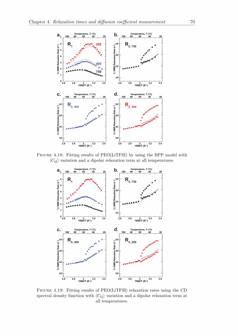
Chapter 4. Relaxation times and diffusion coefficient measurement 70
0
1
2
3
4
5
6
7
2.6 2.8 3 3.2 3.4
100 80 60 40 20
103
102
101
100
Temperature, T (°C)
7L
i N
MR
Re
lax
ati
on
Ra
te (
s-1)
1000/T (K-1)
2.6 2.8 3 3.2 3.4
100 80 60 40 20
103
102
101
100
Temperature, T (°C)
7L
i N
MR
Re
lax
ati
on
Ra
te (
s-1)
1000/T (K-1)2.6 2.8 3 3.2 3.4
100 80 60 40 20
103
102
101
100
Temperature, T (°C)
7L
i N
MR
Re
lax
ati
on
Ra
te (
s-1)
1000/T (K-1)
2.6 2.8 3 3.2 3.4
100 80 60 40 20Temperature, T (°C)
7L
i N
MR
Re
lax
ati
on
Ra
te (
s-1)
1000/T (K-1)
a. b.
c. d.
R1
R2, 400
R2, 750
R2, 200
750
400
200
Figure 4.18: Fitting results of PEO(LiTFSI) by using the BPP model with〈CQ〉 variation and a dipolar relaxation term at all temperatures.
0
1
2
3
4
5
6
7
2.6 2.8 3 3.2 3.4
100 80 60 40 20
103
102
101
100
Temperature, T (°C)
7L
i N
MR
Re
lax
ati
on
Ra
te (
s-1)
1000/T (K-1)
2.6 2.8 3 3.2 3.4
100 80 60 40 20
103
102
101
100
Temperature, T (°C)
7L
i N
MR
Re
lax
ati
on
Ra
te (
s-1)
1000/T (K-1)2.6 2.8 3 3.2 3.4
100 80 60 40 20
103
102
101
100
Temperature, T (°C)
7L
i N
MR
Re
lax
ati
on
Ra
te (
s-1)
1000/T (K-1)
2.6 2.8 3 3.2 3.4
100 80 60 40 20Temperature, T (°C)
7L
i N
MR
Re
lax
ati
on
Ra
te (
s-1)
1000/T (K-1)
a. b.
c. d.
R1
R2, 400
R2, 750
R2, 200
Figure 4.19: Fitting results of PEO(LiTFSI) relaxation rates using the CDspectral density function with 〈CQ〉 variation and a dipolar relaxation term at
all temperatures.

Chapter 4. Relaxation times and diffusion coefficient measurement 71
be described by a normalized and discrete sum of exponential functions,[64] and
therefore, the spectral density function J can be written:
J (ω, τi, xij...) =∑
i
Λi (τi, xi1, xi2, ...)2τi
1 + ω2τ 2i
(4.13)
where Λi (τi, xi1, xi2, ...) is the weight of the ith exponential correlation function
characterized by the correlation time τi.
This strategy has been often used in NMR, especially for the correlation function
describing the fluctuations of dipolar interactions stemming from internal bond
motions and molecular tumbling in molecules.[70] In our case, we assumed that
the quadrupolar interaction fluctuates at three different timescales:
a. Very fast motions (e.g. vibrations) over sub-nanosecond timescales partly av-
erage 7Li quadrupolar couplings, and therefore are reflected in the temperature-
dependent pre-averaged⟨
C2Q
⟩
[111]
b. Fluctuations in the coordination polyhedron of lithium ions to neighboring
oxygen atoms and the concerted motion of statistical or Kuhn’s segments of
the polymer chains lead to partial averaging of the quadrupolar interaction,
this averaging is described by an order parameter S2 -i.e. the proportion
of quadrupolar interaction that remains to be averaged at the end of this
process- and a characteristic time τ1.
c. The quadrupolar interaction is completely averaged over a longer timescale
τ2, as the lithium has moved to an environment with a completely different
EFG orientation. Complete reorientation of the Kuhn’s segment is expected
to occur on a slower timescale as our polymers are entangled, having a mo-
lar mass larger than the critical molecular mass (around 5000 g/mol for
PEO[115]).
Figure 4.20 shows a simple model which depicts the influence of oxygen coordi-
nation around Li+. As the oxygen atoms get close to Li+, the electron cloud of
Li+ is deformed in the Li-O direction. This assumption was similar to Chung’s
study, [116] as they have found the changing of EFG distribution when passing
from unstretched to stretched polymer. This changing was implied by the change
of Li-O bond angle and lengths upon stretching the polymer.

Chapter 4. Relaxation times and diffusion coefficient measurement 72
-+
-
+
+
+
-+
-
+
+
+-+
-
+
+
+
-+
-+
+
+
a. b. c.
Vibration Fluctuation
1 2
Complete reorientation
Figure 4.20: Modeling of the fluctuations of the quadrupolar interaction atthree different timescales
0
0.2
0.4
0.6
0.8
1.0
CQ2
1-S2
S2
t
Co
rre
lati
on
fu
nc
tio
n,
C(t
)
sub ns
Figure 4.21: Correlation function’s representation diagram of three differenttimescales.
The correlation function describing these two last averaging processes can therefore
be written as (see figure 4.21):
C (t) =[
(
1 − S2)
exp(−t
τ1
)
+ S2]
exp(−t
τ2
)
(4.14)
And the corresponding spectral density is given by:
J (ω) =(1 − S2) τ12
1 + ω2τ 212
+S2τ2
1 + ω2τ 22
(4.15)
with1
τ12
=1
τ1
+1
τ2
≈ 1
τ1
(4.16)
if τ2 ≫ τ1.
⟨
C2Q
⟩
, τ1, τ2 and S2 parameters retrieved from the relaxation data are shown in
figure 4.24, for both PEO(LiTFSI) and PS-PEO(LiTFSI)-PS. In figures 4.22 and

Chapter 4. Relaxation times and diffusion coefficient measurement 73
0
1
2
3
4
5
6
7
2.6 2.8 3 3.2 3.4
100 80 60 40 20
103
102
101
100
Temperature, T (°C)
7L
i N
MR
Re
lax
ati
on
Ra
te (
s-1)
1000/T (K-1)
2.6 2.8 3 3.2 3.4
100 80 60 40 20
103
102
101
100
Temperature, T (°C)
7L
i N
MR
Re
lax
ati
on
Ra
te (
s-1)
1000/T (K-1)2.6 2.8 3 3.2 3.4
100 80 60 40 20
103
102
101
100
Temperature, T (°C)
7L
i N
MR
Re
lax
ati
on
Ra
te (
s-1)
1000/T (K-1)
2.6 2.8 3 3.2 3.4
100 80 60 40 20Temperature, T (°C)
7L
i N
MR
Re
lax
ati
on
Ra
te (
s-1)
1000/T (K-1)
750
400
200R1
R2, 400
R2, 750
R2, 200
R2,slow
R2,fast
R2
Figure 4.22: Fitting results of PEO(LiTFSI) by using the new relaxationmodel with 〈CQ〉 variation and dipolar relaxation term at all temperatures.
0
1
2
3
4
5
6
7
2.6 2.8 3 3.2 3.4
100 80 60 40 20
103
102
101
100
Temperature, T (°C)
7L
i N
MR
Re
lax
ati
on
Ra
te (
s-1)
1000/T (K-1)
2.6 2.8 3 3.2 3.4
100 80 60 40 20
103
102
101
100
Temperature, T (°C)
7L
i N
MR
Re
lax
ati
on
Ra
te (
s-1)
1000/T (K-1)2.6 2.8 3 3.2 3.4
100 80 60 40 20
103
102
101
100
Temperature, T (°C)
7L
i N
MR
Re
lax
ati
on
Ra
te (
s-1)
1000/T (K-1)
2.6 2.8 3 3.2 3.4
100 80 60 40 20Temperature, T (°C)
7L
i N
MR
Re
lax
ati
on
Ra
te (
s-1)
1000/T (K-1)
750
400
200R1
R2, 400
R2, 750
R2, 200
R2,slow
R2,fast
Figure 4.23: Fitting results of PS-PEO(LiTFSI)-PS by using the new relax-ation model with 〈CQ〉 variation and dipolar relaxation term at all temperatures.

Chapter 4. Relaxation times and diffusion coefficient measurement 74
25
35
45
55
CQ2
Q2 >
(kH
z)
1000/T (K-1)
Temperature, T (°C)100 80 60 40 20
2.6 2.8 3 3.2 3.4
1000/T (K-1)
Ord
er
Para
mete
r, S
2
0
0.2
0.4
0.6
0.8
1
S2
Temperature, T (°C)100 80 60 40 20
2.6 2.8 3 3.2 3.4
100 80 60 40 20
2.6 2.8 3 3.2 3.4
100
101
102
Co
rrela
tio
n t
ime,
1 &
2 (
ns)
1000/T (K-1)
Temperature, T (°C)
Dip
ola
r R
ela
xati
on
Term
, R
DD (
Hz)
1000/T (K-1)
Temperature, T (°C)
RDD
100 80 60 40 20
2.6 2.8 3 3.2 3.4100
101
102
Figure 4.24: The parameters
√
⟨
C2Q
⟩
, τ1 and τ2, S2 and RDD fitted from the
measured relaxation rates in PEO(LiTFSI)( ) and PS-PEO(LiTFSI)-PS(N).The lines are guides for the eyes, and the activation energies (see table 4.2)
were calculated for τ1 and τ2 using an Arrhenius law.
4.23, the relaxation rates obtained by adjusting the⟨
C2Q
⟩
, τ1, τ2, S2 and RDD
parameters (numerical results shown in appendix A) are shown as lines and fit
very well with the experimental data.
Table 4.2: Activation energy calculated (kJ/mol) for τ1 and τ2 using an Ar-rhenius law.
PEO(LiTFSI) PS-PEO(LiTFSI)-PS
τ1 τ2 τ1 τ2
Below TM 7.37 ± 0.31 41.71 ± 1.65 1.51 ± 0.70 46.80 ± 0.87
Above TM 11.40 ± 0.95 11.63± 1.27 24.32 ± 0.12 0
Below the melting temperature,√
⟨
C2Q
⟩
decreases as the temperature increases
for both PEO and PS-PEO(LiTFSI)-PS, reflecting the increase in the amplitude

Chapter 4. Relaxation times and diffusion coefficient measurement 75
of fast motions as the temperature rises. Above the melting temperature, the de-
crease of√
⟨
C2Q
⟩
stops at around 27 kHz for PEO and 30 kHz for PS-PEO(LiTFSI)-
PS. When the PEO phase is melted, this indicates that no further averaging of
the EFG is possible over this short timescales, and no increase in the amplitude
of local motions is observed. A longer time is needed to further average the EFG,
and this requires another source of EFG fluctuation, i.e. most likely a change
in the oxygen coordination layer or reorientation of the EFG following concerted
polymer chain motions.
Such a change is expected to occur over a time corresponding to τ1. τ1 is found at
around 2-3 ns below the melting temperature, and decreases to 0.5-0.8 ns above the
melting temperature. The τ1 curve can easily be fitted with an Arrhenius law where
τ = τ0 exp(Ea/RT ), providing activation energies at 7.37 kJ/mol and 11.40 kJ/mol
before and after melting respectively, confirming that it is indeed a thermally
activated process. The low activation energy at below the melting temperature
may result from the restriction of motion imposed by the rigidity of the polymer
structure below the melting temperature. Although over such timescales, the
Mean Square Displacement (MSD) is supposed to follow a subdiffusive law, [92] it
is interesting to compute√
〈R2〉 using a diffusive behavior, i.e.:
⟨
R2⟩
= 6Dτc (4.17)
where D is the diffusion coefficient we measured in the same conditions. The
results are shown in figure 4.25a. In this case, the true value of√
〈R2〉 will be larger
than the one computed assuming a diffusive behavior. Such a strategy cannot be
applied to PEO(LiTFSI) below the melting temperature as we expect that some
PEO may be crystallized and therefore, as diffusion occurs in the glassy domains,
the self-diffusion coefficient is measured over 1-2 µm and therefore influenced by
the tortuosity of the glass domains. Hence, D cannot be easily related to motion
at smaller lenghtscale. A similar problem occurs for PS-PEO(LiTFSI)-PS because
of the presence of PS domains.
Fluctuations of the EFG occurring over this timescale can therefore be associ-
ated with a displacement of the Li+ during τ1:√
〈R2〉 ranges between 1 and 2
Å when calculated for τ1. Such a displacement could easily be observed follow-
ing rearrangements of the oxygen coordination layer or reorientation of the poly-
mers which are coordinated to Li+. The latter has been detected with neutron
spin-echo spectrometry,[97] while the former is expected to occur over a 0.1 to 1

Chapter 4. Relaxation times and diffusion coefficient measurement 76
100 90 80 70 60
2.7 2.8 2.9 3.00
2
4
6
8100 80 60 40 20
2.6 2.8 3.0 3.2 3.410-10
10-9
10-8
10-7
10-6
1000/T (K -1)
Temperature, T (°C) Temperature, T (°C)(a) (b)
Co
rre
lati
on
tim
e,
c (
s)
Dis
pla
ce
me
nt,
R (
Å)
2.5
1000/T (K -1)
Figure 4.25: a. Displacement√
〈R2〉 of Li+calculated from Eq. 4.17, N:calculated using τ1, : calculated using τ2; b. The time τinter between interchainjumps for Li+ in PEO(LiTFSI), calculated using [93]. The lines are guides for
the eyes.
ns timescale.[96] Similarly,[117] in polymer electrolyte PEO10LiTFSI, the authors
have shown that the hopping of Li+ from a cage formed by several PEO units
to an alternative cage takes roughly 1 ns, and the residence time of Li+ within
a cage is around 4-7 ns. Both phenomena are expected to be strongly correlated
and both contribute to the fluctuation of the quadrupolar interaction tensor.
The results for τ2 show a correlation time that starts at 250 ns at low temperature,
decay towards 37 ns at the melting temperature with an activation energy of 41.71
kJ/mol. Above the melting temperature, in PEO(LiTFSI), the long correlation
time decays sharply, down to 6.6 ns and decays to 4.3 ns at 100 with an ac-
tivation energy of 11.63 kJ/mol. A similar calculation can be made with τ2, and
yields√
〈R2〉 ranging between 4 to 6 Å closing to the expected length of Kuhn’s
segments in PEO, at 2.5 monomeric units. It would therefore make sense that
the complete averaging of the EFG occurs when Li+ has diffused over a compa-
rable lengthscale. Interestingly, crystal structures of PEO:LiAsF6 complexes [118]
found some lithium channels surrounded by a double PEO helix, with lithium
sites separated by 4.5-5 Å distances. Although the lithium concentration is lower
in our systems, it is interesting to note that such a distances could correspond
well with the distance travelled by Li+ which had their oxygen coordination layer
renewed and progress towards the next site along the double PEO helix. These
studies based on molecular dynamics,[92] with polymer electrolyte PEOnLiTFSI
(n = 7.5, 10, 20, 39; Mw = 2380 g/mol) at temperatures ranging between 120 and

Chapter 4. Relaxation times and diffusion coefficient measurement 77
150 , the authors have pointed out by using MD simulation that the interseg-
mental hops in the range from 5 to 8 Å, and at lower temperature it tends to have
longer intersegmental hopping length. Therefore, there is good agreement between
the time and length scales we measure, and what was observed in previous studies.
Moreover, the order parameter S2 (which describes the proportion of the quadrupo-
lar interaction that has to be averaged over τ2) is fairly high (0.9) at low tempera-
ture and decays fast below melting temperature. An order parameter of 0.9 corre-
sponds to the averaging obtained by a fluctuation of ±21° amplitude of the EFG
axis around its average orientation. [119] After melting, the decay slows down to
0.2 (±72°), indicating that 55% of the quadrupolar interaction is averaged during
τ1, and the rest (45%) is averaged during τ2.
The comparison with PS-PEO(LiTFSI)-PS is very interesting: first, the√
⟨
C2Q
⟩
parameter is systematically higher for PS-PEO(LiTFSI)-PS as the PS domains are
crystallized over the whole temperature range, and may limit the amplitude of fast
PEO segmental motions. Below the melting temperature, the S2 parameter are
similar, although after melting, S2 measured in PS-PEO(LiTFSI)-PS has a similar
decline but toward larger value (0.3 or ±65°) that may be due to reduced motion
caused by the rigidity induced by PS domains. The striking difference concerns
τ2, which does not undergo the sharp decline upon melting the PEO domains,
although it is similar to τ2 measured in PEO(LiTFSI) below the meting temper-
ature, with an activation energy of 46.80 kJ/mol. This may be linked with the
fundamental difference between the PS-PEO(LiTFSI)-PS and the PEO(LiTFSI)
polymers. The PEO chains in PS-PEO(LiTFSI)-PS are anchored to rigid PS
chains, and therefore, these slow motions cannot be accelerated unless PS is also
melted. This has a clear implication for NMR measurements: the transverse re-
laxation of 7Li stays multi exponential beyond the melting of PEO domains. The
short correlation time τ1 is nearly constant at low temperatures (activation energy
of 1.51 kJ/mol), which may be linked with the confinement effect: the presence of
PS domains inhibits the crystallization of PEO domains in which Li+ move inside
tunnels created by parallel polymer chains,[31] so that the Li+ motion is easier
than in neat PEO. After melting, τ1 declines with an activation energy of 24.32
kJ/mol with values close to those of PEO(LiTFSI). The dipolar coupling term is
very similar in both polymers below the melting temperature, however, above the
melting temperature, the dipole-dipole term shows a plateau at 10 Hz, which may
be due again to the effect PS domains. Thus, it seems that the lithium motions are

Chapter 4. Relaxation times and diffusion coefficient measurement 78
constantly slowed down in PS-PEO(LiTFSI)-PS, seemingly due to the restrictions
in motion imposed by the presence of rigid PS domains. This is illustrated in the
correlation functions of the fluctuations of 7Li quadrupolar interactions that are
shown in figure 4.26.
Co
rre
lati
on
Fu
nc
tio
n o
f M
oti
on
Time, t (ns)10-1 100 101 102 103
10-3
10-2
10-1
100
25°C
43°C
62°C85°C
Figure 4.26: Correlation functions describing the fluctuations of the7Li quadrupolar interaction at various temperatures. The correlation functionfor PEO(LiTFSI)(continuous line) shows a systematically faster decay than in
PS-PEO(LiTFSI)-PS (dashed line).
The dipole-dipole term slowly decays as temperature increases, and becomes very
weak above the melting temperature, as expected as the mobilities of the lithium
ions increase and the reorientation of CH bonds becomes faster at higher tem-
peratures. The dipolar coupling term is very similar in both polymer below TM,
however, above TM, the dipole-dipole term shows a plateau at 10 Hz, which may
be due to again to the effect of PS domains.
Maitra et al. [93] found a relationship between the diffusion coefficient and the
mean square end-to-end distance of a polymer chain R2e, the correlation time τintra
(Li+ moves along one chain from head to tail), τchains (Li+ moves cooperatively
with the chains), τinter (Li+ jumps between the chains). Figure 4.27 depicts these
three different timescales. In our case, τchains is very long due to the long PEO
chain. τinter can be calculated by:
τinter =R4
e
(6π)2 D2τintra
(4.18)

Chapter 4. Relaxation times and diffusion coefficient measurement 79
+
inter
intrachains
Figure 4.27: Three different timescales of Li+ motion in polymers were dividedby Borodin et al. [92] : τintra (Li+ moves along one chain from head to tail),τchains (Li+ moves cooperatively with the chains), τinter (Li+ jumps between
the chains) (figure adapted from ref [93])
where R2e is N × L2 with N the number of units (2272 units), L is the distance
between O-O in crystal of (G2)2:LiTFSI [114] is 2.578 Å. τintra was calculated by
τ2, because each Li+ coordinates with 4-5 oxygens (or 4.5 in average) then the
time it takes to go from head to tail is τintra = N2
4.52 τ2. Figure 4.25b shows the τinter
values calculated from equation 4.18.
Do et al. [117] have studied Li+ transport in PEO by neutron spin-echo(NSE),
dielectric spectroscopy and molecular dynamics simulation, showing the important
role of the Li+ hopping process in contributing to macroscopic conductivity.
Golodnitsky et al. [120] have proposed that the conductivity of Li+ in PEO-based
polymer electrolytes below the melting temperature may be due to ’interchain’
hopping. Moreover, Maitra et al. [93] have shown that τinter ∝ N0. Considering
that the correlation times we measured have activation energies which are lower
than the activation energy found for diffusion, it may well be possible that the
limiting process for macroscopic diffusion is the inter-chain hopping motion. This
could explain why spinning the sample increase the activation energy of diffusion
although the relaxation properties seem unaffected by pressure. In this case, spin-
ning the sample may change the relative orientations of polymer chains and make
the inter-chain jumps more difficult.
4.4 Conclusion
The Li+ motion were characterized by both NMR relaxation and PFG-NMR dif-
fusion experiments. The relaxation times characterizing Li+ motion showed that
the quadrupolar interaction fluctuates at three different timescales, and for two of

Chapter 4. Relaxation times and diffusion coefficient measurement 80
them, correlation times can be extracted using a simple model for motion. The
relaxation analysis clearly show that the Li+ dynamics are slowed down in PS-
PEO(LiTFSI)-PS compared to PEO(LiTFSI). From the characteristic timescale
for the averaging of the quadrupolar interaction and the self-diffusion coefficients,
the characteristic time τinter between interchain jumps can be estimated experi-
mentally.

Chapter 5
Polymer electrolytes in ultra thin
film battery
5.1 Introduction
In this part, we will discuss about the use of polymer electrolytes in ultra-thin
battery. This project is a collaboration between the laboratory Physico Chimie de
Matériaux et des Electrolytes pour l’Energie (PCM2E) in Tours and the CEMHTI
laboratory.
Porous solid polymer electrolytes (PSPE) are one of the SPEs which are used in
high energy batteries. [121] The ionic conductivity of PSPE mainly depends on
the conductivity of the electrolyte entrapped in the pores of the membranes. [122]
Microporous polymer electrolytes can feature high ionic conductivities and high
mechanical strengths. [123]
PVdF (Vinylidene fluoride) and its copolymer (PVdF with hexafluoropropylene)
PVdF-HFP are good candidates as battery electrolytes. Therein, PVdF-HFP has
many advantages such as lower crystallinity, high solubility, lower glass transition
temperature than its homogeneous counterpart PVdF. [124, 125]
Lalia et al. [126] improved the ionic conductivity by adding ionic liquids (IL) into
PVdF-HFP polymers. Furthermore, IL are non-volatile, have large ionic conduc-
tivities and excellent thermal, chemical and electrochemical stabilities. [127]
81

Chapter 5. Ultra thin film battery 82
In order to enhance ionic conductivity, mechanical and thermal properties of
PVdF-based polymer electrolytes, polymer blends may also be used. [128] Xi
et al. [129] have shown that the addition of polyoxyethylene (POE, corresponding
to polymer with shorter chains than PEO) to PVdF can improve the pore con-
figuration (pore size, pore connectivity) leading to an enhancement of their ionic
conductivity. However, the mechanical strength of this polymer is lower than the
one observed for pure PVdF. Chung et al. [130] added PEG to PVdF-HFP and
reported that it can increase the porosity and conductivity of the PVdF-HFP net-
work. Cheng et al. [131] designed a new polymer electrolyte based on PVdF-HFP
with PEG acting like plasticizer to increase the flexibility while PEGDMA is in-
troduced to reinforce the PVdF-HFP matrix. The combination of %wt of each
polymer is crucial to control the flexibility, tensile modulus and porosity of poly-
mer samples. Depending on the PEG:PEGDMA ratio, the mechanical strength
decreases while the ionic conductivity increases.
However, the PVdF-HFP membranes show very poor retention of the liquid phase
at high temperature (60 ). POE polymers are known for their electrostatic in-
teractions (Van der Waals) with ions. Therefore, mixing cross-linked POE with
PVdF-HFP is expected to improve its retention of ionic liquid while keeping the
transport properties of PVdF-HFP.
In this work, we will study the diffusion process and relaxation times of hybrid
polymer electrolytes. A set of polymer electrolytes were synthesized including:
• A PVdF-HFP based electrolyte with addition of IL Pyr13FSI and LiTFSI
• A PEGDM/PEGM cross-linked polymer with LiTFSI dissolved in Pyr13FSI
• A mixture of PVdF-HFP and PEGM(Poly ethyleneglycol methyl ether methacry-
late)/PEGDM (Poly ethyleneglycol dimethacrylate) to form a semi-interpenetrated
(SRIP) network [132]
All synthesis were performed by Victor CHAUDOY in the PCM2E laboratory at
the University François Rabelais of Tours.

Chapter 5. Ultra thin film battery 83
O
O
O
On
O
O
O
n
nF F pF CF3
F F
PEGDM PEGM
N+
N(SO2F)
2-
Pyr13
FSI
N-methyl-N-propylpyrrolidinium bis(fluorosulfonyl)imide
Poly ethyleneglycol dimethacrylate (Mn = 550) Poly ethyleneglycol methyl ether methacrylate (M
n = 475)
Poly(vinylidene fluoride-co-hexafluoropropylene)
PVdF-HFP
PVdF-HFP structure was adapted from Sigma-Aldrich
Figure 5.1: Molecule structure of materials used to prepare the polymer elec-trolytes.
5.2 Experiments
An artist’s view of the structure of the PH based on linear PVdF-HFP and POE
samples are shown in figures 5.2 and 5.3, respectively. In this sample, crosslinked
PEGDM maintain the polymer network while the domains and pendant chains
of PEGM are expected to help the flexibility of the chains and the mobility of
the electrolyte species. Adding PEGM is known to lower the glass transition
temperature Tg which favors higher Li+ mobility and ionic conductivity. [133]
Figure 5.4 presents the SRIP gel polymer electrolyte. In SRIP, the PEGDM/PEGM
polymer was expected to limit the syneresis (expulsion of liquid outside the poly-
mer matrix) of PVdF-HFP. The influence of the PEGM:PEGDM ratio on diffusion
coefficients in SRIP sample will be examined. The of IL was kept around 80% (%
wt) for every samples. The composition of prepared samples is shown in table 5.1.
5.3 Results and discussions
Figure 5.5 shows the diffusion coefficients of cation and anion of samples in function
of LiTFSI concentration in PH and SRIP(ratio PEGM:PEGDM-4:1) samples.

Chapter 5. Ultra thin film battery 84
PVdF-HFP
Figure 5.2: PH sample: only PVdF-HFP with IL PyrFSI and salt LiTFSI(©Victor Chaudoy - Université de Tours)
PEGDM network
Cross-linked node
PEGM pendant chain
Permit to increase mobility
Figure 5.3: POE sample:PEGDM/PEGM crosslinked with IL PyrFSI and saltLiTFSI (©Victor Chaudoy - Université de Tours)
PEGDM network
Cross-linked node
PVdF-HFP
PEGM pendant chain
Permit to increase mobility
Figure 5.4: SRIP sample: the linear chain PVdF-HFP is tangled in networkPEGM/PEGDM. There is no chemical link between PVdF-HFP and network
PEGM/PEGDM (©Victor Chaudoy - Université de Tours)

Chapter 5. Ultra thin film battery 85
Table 5.1: The composition of samples
Ref Name PVdF HFP PEGM PEGDM Pyr13FSI+LiTFSI x
% wt M (mol/l)
107A PH 1,3 20 0 0 80 1.3
109C PH 1M 20 0 0 80 1
97C PH 0,6M 20 0 0 80 0.6
116A SRIP 0,6M 15 4 1 80 0.6
76F SRIP 1M 15 4 1 80 1
109A SRIP 1,3M 15 4 1 80 1.3
110D SRIP 1,9M 15 4 1 80 1.9
97E SRIP 2,8M 15 4 1 80 2.8
97F SRIP 3,2M 15 4 1 80 3.2
109B SRIP 1,3M4% 15 1 4 80 1.3
107F SRIP 1,3M5% 15 0 5 80 1.3
110B POE 1,3M 0 16 4 80 1.3
0.6 1 1.3 1.9 2.8 3.2
Concentration, x (M)
Dif
fusio
n C
oeff
icie
nt,
D (
m2/s
)
0.6 1 1.3
10
10
Figure 5.5: Diffusion coefficients of Li+( ), Pyr+13(), TFSI−(N) and FSI−(⋆)
of PH (left), SRIP (right) as a function of LiTFSI concentration x (M). Thelines were guided for eyes

Chapter 5. Ultra thin film battery 86
Figure 5.6: SEM micrographs of the PVdF-HFP membrane (PH sample with-out IL and LiTFSI)
In the PH samples, the self-diffusion coefficients of Li+ decrease with the LiTFSI
concentration from 0.6 to 1.3 M when diffusion coefficients of Pyr+13 slightly increase
from 1 to 1.3 M. On the other hand, diffusion coefficients of TFSI− and FSI−
slightly decrease with increasing concentrations of LiTFSI (from 1 to 1.3 M) in
the PH samples. Figure 5.6 shows the SEM micrographs of PH samples, the porous
structure is easily seen. Therefore, the IL can swell inside these pores leading to
a high conductivity.
FSI− has the highest diffusion coefficient followed by Pyr+13 and TFSI−. Li+ is the
slowest, regardless of its size as Li+ are coordinated to FSI−and/or TFSI−anions
which slow its diffusion to a larger extent than Pyr+13. [134] Moreover, TFSI− is
bulkier than FSI− [135], explaining why TFSI− diffuses slower than FSI−. Further-
more, as Li+ tends to be coordinated to anions, an increase in Li+ concentration
leads to an increase in the self-diffusion coefficient of Pyr+13 and in the viscosity
of the solution, while the diffusion coefficients of Li+, FSI− and TFSI− decrease.
[134] It should be noted that the quantity of ionic liquid is also important for the
diffusion of species. The increase of LiTFSI concentration leads to the decrease of
quantity of ionic liquid because the % wt of Pyr13FSI+LiTFSI was kept the same
for every samples. Therefore, the decrease of diffusion coefficients of species must
be considered to result from several causes.
In the SRIP samples, the self-diffusion coefficient of Li+ reaches its maximum
for a LiTFSI concentration of 1.3 M. This is in contrast with the PH samples
(over the LiTFSI concentration range 0.6-1.3 M). It may be explained by the
presence of POE. When one adds POE, part of the Li+ can be coordinated by the
oxygen atoms of the POE part (see table 5.2 for the number of available oxygens
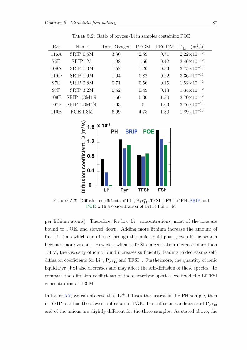
Chapter 5. Ultra thin film battery 87
Table 5.2: Ratio of oxygen/Li in samples containing POE
Ref Name Total Oxygen PEGM PEGDM DLi+ (m2/s)
116A SRIP 0,6M 3.30 2.59 0.71 2.22×10⁻¹²
76F SRIP 1M 1.98 1.56 0.42 3.46×10⁻¹²
109A SRIP 1,3M 1.52 1.20 0.33 3.75×10⁻¹²
110D SRIP 1,9M 1.04 0.82 0.22 3.36×10⁻¹²
97E SRIP 2,8M 0.71 0.56 0.15 1.52×10⁻¹²
97F SRIP 3,2M 0.62 0.49 0.13 1.34×10⁻¹²
109B SRIP 1,3M4% 1.60 0.30 1.30 3.70×10⁻¹²
107F SRIP 1,3M5% 1.63 0 1.63 3.76×10⁻¹²
110B POE 1,3M 6.09 4.78 1.30 1.89×10⁻¹³
0
0.4
0.8
1.2
1.6 x 10⁻¹¹
Dif
fus
ion
co
eff
icie
nt,
D (
m2/s
)
Li+ Pyr+ TFSI- FSI-
PH SRIP POE
Figure 5.7: Diffusion coefficients of Li+, Pyr+13, TFSI−, FSI−of PH, SRIP and
POE with a concentration of LiTFSI of 1.3M
per lithium atoms). Therefore, for low Li+ concentrations, most of the ions are
bound to POE, and slowed down. Adding more lithium increase the amount of
free Li+ ions which can diffuse through the ionic liquid phase, even if the system
becomes more viscous. However, when LiTFSI concentration increase more than
1.3 M, the viscosity of ionic liquid increases sufficiently, leading to decreasing self-
diffusion coefficients for Li+, Pyr+13 and TFSI−. Furthermore, the quantity of ionic
liquid Pyr13FSI also decreases and may affect the self-diffusion of these species. To
compare the diffusion coefficients of the electrolyte species, we fixed the LiTFSI
concentration at 1.3 M.
In figure 5.7, we can observe that Li+ diffuses the fastest in the PH sample, then
in SRIP and has the slowest diffusion in POE. The diffusion coefficients of Pyr+13
and of the anions are slightly different for the three samples. As stated above, the

Chapter 5. Ultra thin film battery 88
0
0.5
1.0
1.5x 10⁻¹¹
Dif
fus
ion
co
eff
icie
nt,
D (
m2/s
)
Li+ Pyr+ TFSI- FSI-
4:1 1:4 0:5
Figure 5.8: Diffusion coefficients of Li+, Pyr+13, TFSI−and FSI−in SRIP sam-
ples with difference ratio of PEGM:PEGDM (4:1, 1:4, 0:5) with an LiTFSIconcentration 1.3 M
largest diffusion coefficient for Li+ is found in the PH sample, as expected as Li+
ions are only coordinated to the anions of the ionic liquid. The higher diffusion
coefficient of Li+ in SRIP than in POE can be explained by the presence of a
porous structure. The IL can swell in the pores where Li+ can diffuse easier than
the case of POE.
The self-diffusion coefficients dependence upon the PEGM:PEGDM ratio in SRIP
samples is shown in figure 5.8. The PEGM:PEGDM ratio does not seem to have
much influence on the Li+ diffusion coefficients in the SRIP samples, while the
diffusion coefficients of Pyr+13 and anions variate slightly. This observation is in
contradiction to what was expected: increasing the PEGM:PEGDM ratio was
supposed to improve the mobility of Li+. Therefore, we can infer that Li+ is
coordinated to oxygens of the PEGDM network and that adding PEGM decreased
the glass transition temperature but do not favor the mobility of Li+.
The 7Li longitudinal and transverse relaxation rates of these samples are shown in
figures 5.9, 5.10, respectively. On the one hand, we observed the mono-exponential
behavior of longitudinal relaxation while transverse relaxation is bi-exponential
(with a 60/40 ratio between the two exponentials) in both SRIP and POE sam-
ples. On the other hand, both transverse and longitudinal relaxations are mono-
exponential in the PH samples.
As shown in chapter 4, the bi-exponentiality of 7Li transverse relaxation is found
in POE(LiTFSI) below the melting temperature.

Chapter 5. Ultra thin film battery 89
0.6 1 1.3 1.9 2.8 3.20.5
0.6
0.7
0.8
0.9
1
Concentration, x (M)
Lo
ng
itu
din
al R
ela
xati
on
rate
, R
1 (
s-1)
Figure 5.9: 7Li longitudinal relaxation rates of PH, SRIP(PEGM:PEGDM-4:1) and POE samples as a function of the LiTFSI concentration. The lines
were guided for eyes.
102
103
0.6 1 1.3 1.9 2.8 3.2Concentration, x (M)
Tra
nsvers
al R
ela
xati
on
rate
, R
2 (
s-1)
101
100
R2, fast
R2, slow
R2, fast
R2, slow
R2
Figure 5.10: 7Li transverse relaxation rates of PH, SRIP(PEGM:PEGDM-4:1)and POE samples as a function of the LiTFSI concentration. The lines were
guided for eyes.

Chapter 5. Ultra thin film battery 90
Therefore, it seems that the local environment of Li+ is modified when adding
PEGDM/PEGM into the PH sample, leading, not only to a decrease of the diffu-
sion coefficient, but also to an increase of the correlation times of the fluctuation of
the Li+ quadrupolar interaction (less mobility at the atomic scale), confirming the
presence of interactions between Li+ and the oxygen atoms of the POE fragments.
5.4 Conclusions
The study of self-diffusion coefficients of electrolyte species provided us with in-
teresting results. The presence of oxygen atoms lead to the coordination of Li+
to them and slowed their diffusion down. In the SRIP samples, the presence of
a porous structure improved the self-diffusion coefficients of Li+ compared to the
POE samples while the Pyr+13 cation and the anions were not strongly influenced.
Adding PEGM/PEGDM to PVdF-HFP (SRIP sample) decreased the self-diffusion
coefficient of Li+ by 20 % compared to the original PH sample. Moreover, the ratio
PEGM:PEGDM has no influence on the diffusion coefficient of Li+ in the SRIP
samples.
The lower diffusion results from coordination effects at the atomic scale, as the
change in relaxation rates of Li+ show an increase in the correlation times of
the fluctuations of the Li+ environment when POE domains are added. This
is clearly seen as transverse relaxation becomes bi-exponential in the POE and
SRIP samples, and confirms what was inferred from the lower conductivities and
the worse battery performance.

Chapter 6
Conclusions and Perspectives
6.1 Conclusions
Solid polymer electrolytes are strong candidates for lithium-metal batteries regard-
less their low ionic conductivities. NMR is very useful for the characterization of
SPEs as it gives the possibility to look at diffusion coefficients at the micron scale,
and at the microscopic motion of Li+ through high-field relaxometry. Although
MAS has many advantages, like reducing the residual dipole-dipole interactions
and susceptibility effects, leading to better resolution, increased sensitivity, and
more homogeneous field gradients, it has some serious side effects due to the cen-
trifugal forces. Although lithium motion at the nanoscale seems unaffected, the
diffusion process seems to be altered by the applied pressure.
Microscopic motion of Li+ was then studied by a high-field relaxometry approach.
Using a "model-free" approach, two timescales are detected for the Li+ motion,
linked with changes in the coordination layer and with the complete averaging of
the quadrupolar interaction, both at the nanosecond timescale, and corresponding
to mean-square displacement over 2-6 Å. Other models failed to reproduce the
data.
Two polymer electrolytes, PEO(LiTFSI) and PS-PEO(LiTFSI)-PS were studied
by diffusion and relaxation. The phase-separated PS-PEO(LiTFSI)-PS has a
slower diffusion, mainly because of the tortuosity of the PEO phase. However,
relaxation rates showed that the presence of PS chains attached at each end of the
91

Chapter 6. Conclusions and Perspectives 92
PEO chain tend to slow the motion of Li+ at the nanosecond timescale. There-
fore, assuming that the motion of Li+ in PEO(LiTFSI) and in the PEO domains
of PS-PEO(LiTFSI)-PS are similar at the atomic level may be wrong. This has
deep implications for the design of block-copolymer electrolytes.
The diffusion and relaxation properties of thin film polymer electrolytes based on
PVdF-HFP were also investigated. Introducing a PEGDM/PEGM network inside
the porosity of PVdF-HFP increase the retention of ionic liquids, however, it also
slows Li+ diffusion down, mainly because Li+ interacts with the oxygen atoms of
these polymer chains.
6.2 Perspectives
Three main perspectives can be considered:
1. Molecular dynamics: First, the understanding of Li+ motion could be en-
hanced by using molecular dynamics (MD) trajectories to retrieve relaxation
properties of 7Li , and check if an agreement can be reached between the
NMR relaxation rates and the motion depicted by MD.
2. New samples, new experiments: Other samples could benefit from the re-
laxation and diffusion analysis, in particular, PSTFSILi-PEO-PSTFSILi is
currently being analyzed in a similar manner. Moreover, the existence of a
"dead zone" close to the PS domains could be probed by NMR correlation
experiments.
3. Magnetic Resonance Imaging (MRI): In situ analysis of the concentration
profiles can be measured by NMR imaging techniques, and would provide
interesting information about the mobility of ions inside an electric field.

Appendix A
Experimental relaxation rates
and calculated parameters
A.1 Calculation method
In this section, we will explain how the calculations were performed at each temper-
ature points simultaneously for three different magnetic fields. For each magnetic
field, the relaxation rates were measured at various temperatures between 25 and
100. As the temperatures are not exactly the same for each spectrometer, we
modelled the data with a polynomial curve to interpolated the experimental data
and obtain for each field, the relaxation rates at exactly the same temperature.
The equations of relaxation rates were shown in Chapter 4. The parameters were
variated to minimize the difference between experimental relaxation rates at each
field and their calculated values using a χ2 minimization method in Maple:
χ2 = a∑
i
(
R1(cal) − R1(exp, i)
R1(exp, i)
)2
+∑
i
(
R2,fast(cal) − R2,fast(exp, i)
R2,fast(exp, i)
)2
+∑
i
(
R2,slow(cal) − R2,slow(exp, i)
R2,slow(exp, i)
)2(A.1)
where a is a weighting parameter fo ensure the fit is correct. The additional a
term compensate the large difference of R1 and R2 values which leads to the local
χ2 minima (see tables A.1 and A.2). In our case, a was set to 10. Equation A.1
93

Appendix . Experiment relaxation rates and calculated parameters 94
was used for the case of PS-PEO(LiTFSI)-PS at all temperature points and for
PEO(LiTFSI) below the melting temperature, while equation A.2 was used for
PEO(LiTFSI) above the melting temperature. i stand for the magnetic field and
takes the following values 4.7 (200 MHz for 1H ), 9.4 (400 MHz for 1H ) and 17.6
T (750 MHz for 1H ).
χ = a∑
i
(
R1(cal) − R1(exp, i)
R1(exp, i)
)2
+∑
i
(
R2(cal) − R2(exp, i)
R2(exp, i)
)2
(A.2)
A.2 Experimental relaxation rates
The longitudinal and transversal relaxation rates are shown in tables A.1 for
PEO(LiTFSI) and A.2 for PS-PEO(LiTFSI)-PS.

App
endix.
Experim
ent
relaxa
tion
rates
and
calcu
lated
para
meters
95
Table A.1: 7Li relaxation rates (s−1) of PEO, where the unit for 1000/T is (K−1)
1000/T R1750 1000/T R1400 1000/T R1200 1000/T R2,slow750 R2,fast750 R2750 1000/T R2,slow400 R2,fast400 R2400 1000/T R2,slow200 R2,fast200 R2200
3.372 0.876 3.372 1.942 3.356 4.260 3.310 62.786 679.569 3.372 113.000 909.000 3.356 71.625 704.176
3.340 0.936 3.310 2.152 3.328 4.570 3.250 42.847 446.309 3.310 94.859 660.946 3.328 69.105 700.378
3.310 1.004 3.250 2.489 3.300 4.810 3.192 30.032 266.386 3.250 55.741 432.526 3.300 49.675 551.846
3.279 1.092 3.221 2.637 3.273 5.130 3.164 31.212 213.610 3.221 46.045 369.549 3.273 45.846 507.949
3.250 1.182 3.192 2.743 3.247 5.380 3.136 26.152 150.664 3.192 38.751 234.852 3.247 36.189 411.435
3.221 1.224 3.164 2.872 3.221 5.490 3.109 25.142 118.464 3.164 31.526 227.169 3.221 31.345 351.335
3.192 1.320 3.136 3.009 3.195 5.680 3.082 23.865 87.418 3.136 25.691 177.368 3.195 26.903 308.567
3.164 1.454 3.109 3.064 3.170 6.020 3.056 19.557 56.491 3.109 21.638 128.833 3.170 26.697 257.945
3.136 1.534 3.082 3.131 3.145 6.020 3.030 21.021 38.201 3.082 18.083 86.580 3.145 19.769 204.456
3.109 1.589 3.056 3.180 3.120 5.920 2.980 10.455 3.056 13.635 50.251 3.120 20.296 174.483
3.082 1.698 3.030 3.164 3.096 6.020 2.931 9.312 3.030 15.883 3.096 16.277 130.429
3.056 1.738 3.005 3.145 3.072 5.950 2.884 8.384 3.005 12.189 3.072 14.890 109.795
3.030 1.828 2.980 3.139 3.049 5.920 2.839 7.807 2.980 11.001 3.049 12.711 62.610
2.980 1.865 2.956 3.053 3.026 5.710 2.794 7.295 2.955 10.597 3.026 10.769 34.339
2.931 1.872 2.931 2.916 3.003 5.320 2.752 6.998 2.931 10.261 3.003 13.382
2.884 1.839 2.908 2.877 2.981 5.260 2.710 6.465 2.908 9.702 2.981 13.046
2.839 1.794 2.884 2.811 2.959 5.050 2.670 6.028 2.884 9.187 2.959 11.774
2.794 1.750 2.861 2.717 2.937 4.900 2.861 8.872 2.937 10.838
2.752 1.690 2.839 2.641 2.915 4.590 2.839 8.280 2.915 10.640
2.710 1.612 2.795 2.475 2.874 4.310 2.794 7.862 2.874 9.160
2.670 1.538 2.752 2.367 2.833 3.920 2.752 7.296 2.833 8.341
2.710 2.199 2.793 3.660 2.710 6.939 2.793 7.933
2.670 2.108 2.755 3.450 2.670 6.557 2.755 7.258
2.717 3.030 2.717 6.626
2.681 2.850 2.681 6.538

App
endi
x.
Exp
erim
ent
rela
xati
on
rate
sand
calc
ula
ted
para
met
ers
96 Table A.2: 7Li relaxation rates (s−1) of PS-PEO(LiTFSI)-PS, where the unit for 1000/T is (K−1)
1000/T R1750 1000/T R1400 1000/T R1200 1000/T R2,slow750 R2,fast750 1000/T R2,slow400 R2,fast400 1000/T R2,slow200 R2,fast200
3.372 1.011 3.372 1.952 3.356 4.121 3.372 215.117 2127.868 3.372 122.100 1709.402 3.356 98.700 936.000
3.340 1.073 3.310 2.176 3.328 4.154 3.340 166.667 1784.446 3.310 84.746 1129.944 3.328 86.500 998.000
3.310 1.135 3.250 2.497 3.300 4.628 3.310 99.681 1079.805 3.250 56.180 645.161 3.300 68.800 828.000
3.279 1.216 3.221 2.657 3.273 4.868 3.279 106.273 1127.040 3.221 39.216 500.000 3.273 62.500 626.000
3.250 1.296 3.192 2.762 3.247 4.916 3.250 63.452 657.412 3.192 31.847 328.947 3.247 48.400 609.000
3.221 1.345 3.164 3.000 3.221 5.308 3.221 65.405 630.146 3.164 26.110 249.377 3.221 37.700 499.000
3.192 1.451 3.136 3.049 3.195 5.217 3.192 41.333 335.503 3.136 19.763 167.785 3.195 32.500 335.000
3.164 1.485 3.109 3.145 3.170 5.672 3.164 41.225 322.079 3.109 16.835 125.471 3.170 29.000 303.000
3.136 1.595 3.082 3.094 3.145 5.795 3.136 27.013 148.640 3.082 21.930 76.923 3.145 23.500 218.000
3.109 1.643 3.056 3.080 3.120 5.975 3.109 26.564 119.992 3.056 20.367 61.350 3.120 19.200 175.000
3.082 1.718 3.034 3.049 3.096 5.826 3.082 22.154 93.500 3.034 20.161 60.976 3.096 17.500 125.000
3.056 1.735 3.005 2.976 3.072 5.953 3.056 17.700 73.669 3.005 21.866 50.251 3.072 16.300 99.400
3.030 1.845 2.980 2.994 3.049 5.767 3.030 16.029 54.435 2.980 19.802 55.866 3.049 13.700 82.200
2.980 1.885 2.956 2.968 3.026 5.498 2.980 14.580 53.286 2.955 17.391 54.348 3.026 14.500 62.000
2.931 1.856 2.931 2.839 3.003 5.482 2.931 14.228 50.398 2.931 16.420 55.556 3.003 13.600 63.800
2.884 1.871 2.908 2.825 2.981 5.218 2.884 13.995 48.768 2.908 17.500 51.900 2.981 13.200 57.100
2.839 1.842 2.884 2.763 2.959 5.234 2.839 11.575 47.668 2.884 16.722 52.083 2.959 14.200 57.700
2.794 1.796 2.861 2.710 2.937 4.985 2.794 11.478 45.508 2.861 15.649 51.813 2.937 13.600 61.400
2.752 1.707 2.839 2.650 2.915 4.706 2.752 11.400 45.840 2.839 15.949 52.632 2.915 12.600 58.500
2.710 1.632 2.795 2.472 2.874 4.347 2.710 11.692 44.369 2.794 15.699 49.505 2.874 12.100 53.100
2.670 1.598 2.793 3.879 2.670 11.811 42.510 2.833 12.100 53.200
2.755 3.508 2.793 14.500 54.400
2.717 3.225 2.755 12.600 52.400
2.681 2.937 2.717 12.300 51.700
2.681 11.400 47.700

Appendix . Experiment relaxation rates and calculated parameters 97
A.3 The parameters calculated from successful
model
The parameters are calculated from the model presented in chapter 4, as seen in
table A.3.

App
endi
x.
Exp
erim
ent
rela
xati
on
rate
sand
calc
ula
ted
para
met
ers
98
Table A.3: Parameters of PEO(LiTFSI) and PS-PEO(LiTFSI)-PS calculated from successful model
PEO(LiTFSI) PS-PEO(LiTFSI)-PS
1000/T (K−1)√
⟨
C2Q
⟩
(kHz) τ1 (ns) τ2 (ns) τinter (ns) S2 RDD(Hz)√
⟨
C2Q
⟩
(kHz) τ1 (ns) τ2 (ns) S2 RDD(Hz)
3.372 44.643 3.227 248.436 0.896 109.987 52.037 2.141 288.214 0.919 135.294
3.340 44.615 3.048 198.899 0.895 80.948 50.913 2.141 257.928 0.909 107.229
3.310 43.625 2.987 171.666 0.884 60.997 49.357 2.141 226.067 0.897 83.439
3.279 42.446 2.956 151.968 0.868 47.712 47.500 2.141 195.172 0.881 64.511
3.250 41.370 2.918 136.115 1902.483 0.849 38.302 45.423 2.141 166.500 0.862 49.835
3.221 39.997 2.857 119.424 0.826 31.906 43.201 2.141 140.718 0.838 38.615
3.192 38.704 2.784 105.810 600.826 0.801 26.785 40.915 2.141 118.181 0.808 30.143
3.164 37.248 2.708 93.916 291.404 0.769 22.508 38.654 2.141 99.027 0.772 23.832
3.136 35.526 2.633 82.803 173.101 0.727 18.816 36.555 2.141 82.645 0.732 19.185
3.109 33.604 2.553 71.746 123.610 0.675 15.557 34.394 2.141 70.817 0.682 15.884
3.082 31.649 2.460 59.977 74.882 0.613 12.640 32.234 2.141 60.344 0.622 13.853
3.056 29.480 2.397 49.287 45.035 0.530 10.116 30.780 2.066 52.553 0.570 11.875
3.030 27.388 2.343 37.399 31.280 0.432 7.893 29.951 1.876 45.045 0.532 11.356
2.980 27.388 0.843 6.644 27.531 0.359 6.039 29.951 1.608 44.440 0.501 10.901
2.931 27.388 0.839 6.644 17.154 0.307 4.983 29.951 1.406 44.440 0.474 10.610
2.884 27.388 0.796 6.412 11.433 0.270 4.429 29.951 1.226 44.440 0.446 10.414
2.839 27.388 0.750 5.971 8.882 0.237 4.177 29.951 1.065 44.440 0.414 10.220
2.794 27.388 0.705 5.626 5.818 0.209 4.017 29.951 0.934 44.440 0.385 10.194
2.752 27.388 0.659 5.280 3.870 0.187 3.886 29.951 0.825 44.440 0.358 10.194
2.710 27.388 0.610 4.855 3.022 0.173 3.744 29.951 0.733 44.440 0.333 10.194
2.670 27.388 0.556 4.306 2.599 0.171 3.558 29.951 0.654 44.440 0.311 10.194

Bibliography
[1] M. Singh, O. Odusanya, G. M. Wilmes, H. B. Eitouni, E. D. Gomez, A. J.
Patel, V. L. Chen, M. J. Park, P. Fragouli, H. Iatrou, N. Hadjichristidis,
D. Cookson, and N. P. Balsara, Macromolecules 40, 4578 (2007).
[2] S. Arumugam, J. Shi, D. P. Tunstall, and C. A. Vincent, Journal of Physics:
Condensed Matter 5, 153 (1993).
[3] M. Kitamura, Y. Hata, H. Yasuoka, T. Kurotsu, and A. Asano, Polymer
Journal 44, 778 (2012).
[4] A. Panday, S. Mullin, E. D. Gomez, N. Wanakule, V. L. Chen, A. Hexemer,
J. Pople, and N. P. Balsara, Macromolecules 42, 4632 (2009).
[5] R. Bouchet, S. Maria, R. Meziane, A. Aboulaich, L. Lienafa, J.-P. Bon-
net, T. N. T. Phan, D. Bertin, D. Gigmes, D. Devaux, R. Denoyel, and
M. Armand, Nature Materials 12, 452 (2013).
[6] M. S. Whittingham, Proceedings of the IEEE 100, 1518 (2012).
[7] J. Qian, W. A. Henderson, W. Xu, P. Bhattacharya, M. Engelhard,
O. Borodin, and J.-G. Zhang, Nature Communications 6, 6362 (2015).
[8] W. Xu, J. Wang, F. Ding, X. Chen, E. Nasybulin, Y. Zhang, and J.-G.
Zhang, Energy & Environmental Science 7, 513 (2014).
[9] M. Dollé, L. Sannier, B. Beaudoin, M. Trentin, and J.-M. Tarascon, Elec-
trochemical and Solid-State Letters 5, A286 (2002).
[10] N. Dudney and B. Neudecker, Current Opinion in Solid State and Materials
Science 4, 479 (1999).
[11] N. J. Dudney, The Electrochemical Society Interface 17, 44 (2008).
99

Bibliography 100
[12] A. Patil, V. Patil, D. W. Shin, J.-W. Choi, D.-S. Paik, and S.-J. Yoon,
Materials Research Bulletin 43, 1913 (2008).
[13] J. Bates, N. Dudney, B. Neudecker, A. Ueda, and C. Evans, Solid State
Ionics 135, 33 (2000).
[14] N. Dudney, J. Bates, and B. Neudecker, in Encyclopedia of Materials: Sci-
ence and Technology (Elsevier BV, 2001) pp. 9302–9306.
[15] N. J. Dudney, Materials Science and Engineering: B 116, 245 (2005).
[16] J. Bates, N. Dudney, G. Gruzalski, R. Zuhr, A. Choudhury, C. Luck, and
J. Robertson, Journal of Power Sources 43, 103 (1993).
[17] X. Yu, J. Bates, G. Jellison, and F. Hart, Journal of The Electrochemical
Society 144, 524 (1997).
[18] M. Liu, S. J. Visco, and L. C. De Jonghe, Journal of The Electrochemical
Society 138, 1891 (1991).
[19] P. E. Trapa, B. Huang, Y.-Y. Won, D. R. Sadoway, and A. M. Mayes,
Electrochemical and Solid-State Letters 5, A85 (2002).
[20] P. E. Trapa, M. H. Acar, D. R. Sadoway, and A. M. Mayes, Journal of The
Electrochemical Society 152, A2281 (2005).
[21] D. Fenton, J. Parker, and P. Wright, Polymer 14, 589 (1973).
[22] M. Armand, J. Chabagno, and M. Duclot, Fast ion transport in solids, edited
by P. Vashishta, J. Mundy, and G. Shenoy (North Holland, Amsterdam,
1979).
[23] J.-M. Tarascon and M. Armand, Nature 414, 359 (2001).
[24] J.-H. Shin, W. A. Henderson, and S. Passerini, Journal of The Electrochem-
ical Society 152, A978 (2005).
[25] R. Agrawal and G. Pandey, Journal of Physics D: Applied Physics 41, 223001
(2008).
[26] F. Gray and M. Armand, in Handbook of Battery Materials (Wiley-Blackwell,
2011) pp. 627–656.

Bibliography 101
[27] S. D. Druger, A. Nitzan, and M. A. Ratner, The Journal of Chemical Physics
79, 3133 (1983).
[28] M. A. Ratner and D. F. Shriver, Chemical Reviews 88, 109 (1988).
[29] C. Berthier, W. Gorecki, M. Minier, M. Armand, J. Chabagno, and
P. Rigaud, Solid State Ionics 11, 91 (1983).
[30] B.-K. Choi and Y.-W. Kim, Electrochimica Acta 49, 2307 (2004).
[31] Z. Gadjourova, Y. G. Andreev, D. P. Tunstall, and P. G. Bruce, Nature
412, 520 (2001).
[32] D. Golodnitsky, E. Livshits, Y. Rosenberg, I. Lapides, and E. Peled, Solid
State Ionics 147, 265 (2002).
[33] M. Marzantowicz, J. Dygas, F. Krok, Z. Florjańczyk, and E. Zygadło-
Monikowska, Electrochimica Acta 53, 1518 (2007).
[34] K. Nagaoka, H. Naruse, I. Shinohara, and M. Watanabe, Journal of Polymer
Science: Polymer Letters Edition 22, 659 (1984).
[35] J. L. Souquet, M. Levy, and M. Duclot, Solid State Ionics 70, 337 (1994).
[36] J. Shi and C. A. Vincent, Solid State Ionics 60, 11 (1993).
[37] J.-F. L. Nest, A. Gandini, and H. Cheradame, British Polymer Journal 20,
253 (1988).
[38] W. H. Meyer, Advanced Materials 10, 439 (1998).
[39] U. Lauter, W. H. Meyer, and G. Wegner, Macromolecules 30, 2092 (1997).
[40] J. Giles, F. Gray, J. MacCallum, and C. Vincent, Polymer 28, 1977 (1987).
[41] F. Alloin, J. Sanchez, and M. Armand, Electrochimica Acta 37, 1729 (1992).
[42] T. Niitani, M. Shimada, K. Kawamura, K. Dokko, Y.-H. Rho, and K. Kana-
mura, Electrochemical and Solid-State Letters 8, A385 (2005).
[43] K. Xu, Chemical Reviews 104, 4303 (2004).
[44] J. L. Schaefer, D. A. Yanga, and L. A. Archer, Chemistry of Materials 25,
834 (2013).

Bibliography 102
[45] L. M. Bronstein, R. L. Karlinsey, B. Stein, Z. Yi, J. Carini, and J. W.
Zwanziger, Chemistry of Materials 18, 708 (2006).
[46] K. L. Mathews, A. M. Budgin, S. Beeram, A. T. Joenathan, B. D. Stein,
U. Werner-Zwanziger, M. Pink, L. A. Baker, W. E. Mahmoud, J. P. Carini,
and L. M. Bronstein, Journal of Materials Chemistry A 1, 1108 (2013).
[47] T. Hamaide and C. Le Deore, Polymer 34, 1038 (1993).
[48] K. Ito, N. Nishina, Y. Tominaga, and H. Ohno, Solid State Ionics 86, 325
(1996).
[49] R. J. Klein and J. Runt, The Journal of Physical Chemistry B 111, 13188
(2007).
[50] R. Bouchet, T. Phan, E. Beaudoin, D. Devaux, P. Davidson, D. Bertin, and
R. Denoyel, Macromolecules 47, 2659 (2014).
[51] Z. Xue, D. He, and X. Xie, Journal of Materials Chemistry A 3, 19218
(2015).
[52] M. H. Levitt, Spin dynamics: basics of nuclear magnetic resonance, Second
edition (John Wiley & Sons, 2008).
[53] R. Böhmer, K. Jeffrey, and M. Vogel, Progress in Nuclear Magnetic Reso-
nance Spectroscopy 50, 87 (2007).
[54] T. Meersmann, Relaxation and Coherenceherent Evolution as Competing
Mechanisms for Coherence Transfer in Nuclear Magnetic Resonance Spec-
troscopy, Ph.D. thesis, University of Lausane (1997).
[55] M. J. Duer, Solid state NMR spectroscopy: principles and applications (John
Wiley & Sons, 2008).
[56] A. Medek, J. S. Harwood, and L. Frydman, Journal of the American Chem-
ical Society 117, 12779 (1995).
[57] M. R. Hansen, R. Graf, and H. W. Spiess, Accounts of Chemical Research
46, 1996 (2013).
[58] T. Asakura and I. Ando, Solid state NMR of polymers, Vol. 84 (Elsevier,
1998).

Bibliography 103
[59] K. Saalwächter and H. Spiess, in Polymer Science: A Comprehensive Refer-
ence (Elsevier BV, 2012) pp. 185–219.
[60] S. Wimperis, Encyclopedia of Magnetic Resonance (2011).
[61] K. Schmidt-Rohr and H. W. Spiess, Multidimensional Solid-State NMR and
Polymers (Academic Press, 1994).
[62] A. G. Palmer III and C. Bracken, in NMR in Supramolecular Chemistry
(Springer, 1999) pp. 171–190.
[63] M. Goldman, Journal of Magnetic Resonance 149, 160 (2001).
[64] P. A. Beckmann, Physics Reports 171, 85 (1988).
[65] N. Bloembergen, E. M. Purcell, and R. V. Pound, Physical Review 73, 679
(1948).
[66] K. Hayamizu, Y. Aihara, and W. S. Price, Journal of Chemical Physics
113, 4785 (2000).
[67] L. G. Werbelow, Encyclopedia of Magnetic Resonance (2011).
[68] L. A. Dissado and R. M. Hill, Nature 279, 685 (1979).
[69] G. Lipari and A. Szabo, Biochemistry 20, 6250 (1981).
[70] G. Lipari and A. Szabo, Journal of the American Chemical Society 104,
4546 (1982).
[71] R. M. Roque-Malherbe, The Physical Chemistry of Materials: Energy and
Environmental Applications (CRC Press, 2010).
[72] M. Kizilyalli, J. Corish, R. Metselaar, et al., Pure and Applied Chemistry
71, 1307 (1999).
[73] W. S. Price, NMR Studies of Translational Motion: Principles and Applica-
tions (Cambridge University Press, 2009).
[74] R. A. K. Bockris, John O’M., Volume 1: Modern Electrochemistry, edited
by J. O. Bockris (Springer US, 1998).
[75] J. Kerr, in Lithium Batteries: Science and Technology (Springer, 2003) pp.
575–622.

Bibliography 104
[76] E. M. Terentjev, P. T. Callaghan, and M. Warner, The Journal of Chemical
Physics 102, 4619 (1995).
[77] W. S. Price, Concepts in Magnetic Resonance 9, 299 (1997).
[78] K. A. Heisel, J. J. Goto, and V. V. Krishnan, American Journal of Analytical
Chemistry 3, 401 (2012).
[79] E. Stejskal and J. Tanner, The Journal of Chemical Physics 42, 288 (1965).
[80] A. Pampel, F. Engelke, D. Groß, T. Oerther, and K. Zick, Spin Report
157-158, 26 (2006).
[81] D. Wu, A. Chen, and C. S. Johnson, Journal of Magnetic Resonance, Series
A 115, 260 (1995).
[82] A. Pampel, D. Michel, and R. Reszka, Chemical Physics Letters 357, 131
(2002).
[83] A. Bielecki and D. P. Burum, Journal of Magnetic Resonance, Series A 116,
215 (1995).
[84] C. Ammann, P. Meier, and A. Merbach, Journal of Magnetic Resonance
(1969) 46, 319 (1982).
[85] I. Kawamura, Y. Degawa, S. Yamaguchi, K. Nishimura, S. Tuzi, H. Saitô,
and A. Naito, Photochemistry and Photobiology 83, 346 (2007).
[86] A. Asano, S. Hori, M. Kitamura, C. T. Nakazawa, and T. Kurotsu, Polymer
Journal 44, 706 (2012).
[87] I. Kawamura, N. Kihara, M. Ohmine, K. Nishimura, S. Tuzi, H. Saitô, and
A. Naito, Journal of the American Chemical Society 129, 1016 (2007).
[88] D. Golodnitsky, E. Livshits, A. Ulus, Z. Barkay, I. Lapides, E. Peled,
S. Chung, and S. Greenbaum, The Journal of Physical Chemistry A 105,
10098 (2001).
[89] J. K. Maranas, in Polymers for Energy Storage and Delivery: Polyelectrolytes
for Batteries and Fuel Cells (American Chemical Society (ACS), 2012) pp.
1–17.

Bibliography 105
[90] Z. Gadjourova, D. Martín y Marero, K. H. Andersen, Y. G. Andreev, and
P. G. Bruce, Chemistry of Materials 13, 1282 (2001).
[91] R. Frech, S. Chintapalli, P. G. Bruce, and C. A. Vincent, Chemical Com-
munications , 157 (1997).
[92] O. Borodin and G. D. Smith, Macromolecules 39, 1620 (2006).
[93] A. Maitra and A. Heuer, Physical Review Letters 98 (2007).
[94] D. Diddens, A. Heuer, and O. Borodin, Macromolecules 43, 2028 (2010).
[95] O. Borodin, G. D. Smith, and R. Douglas, The Journal of Physical Chem-
istry B 107, 6824 (2003).
[96] O. Borodin and G. D. Smith, Macromolecules 33, 2273 (2000).
[97] G. Mao, M.-L. Saboungi, D. L. Price, M. Armand, F. Mezei, and S. Pouget,
Macromolecules 35, 415 (2002).
[98] Y. Wang, A. L. Agapov, F. Fan, K. Hong, X. Yu, J. Mays, and A. P.
Sokolov, Physical Review Letters 108, 088303 (2012).
[99] K. Hayamizu, Y. Aihara, and W. S. Price, Electrochimica Acta 46, 1475
(2001).
[100] D. Davidson and R. Cole, The Journal of Chemical Physics 19, 1484 (1951).
[101] M. Zeidler, Berichte der Bunsen-Gesellschaft für Physikalische Chemie 95,
971 (1991).
[102] A. Friedrich, A. Dölle, and M. D. Zeidler, Magnetic Resonance in Chemistry
41, 813 (2003).
[103] S. Bhattacharja, S. Smoot, and D. Whitmore, Solid State Ionics 18-19,
Part 1, 306 (1986).
[104] W. Gorecki, M. Jeannin, E. Belorizky, C. Roux, and M. Armand, Journal
of Physics: Condensed Matter 7, 6823 (1995).
[105] T. H. Epps, T. S. Bailey, R. Waletzko, and F. S. Bates, Macromolecules 36,
2873 (2003).

Bibliography 106
[106] E. Beaudoin, T. N. Phan, M. Robinet, R. Denoyel, P. Davidson, D. Bertin,
and R. Bouchet, Langmuir 29, 10874 (2013).
[107] R. O. Ebewele, Polymer Science and Technology (CRC Press, 2000).
[108] L. Shen and Z. Chen, Chemical Engineering Science 62, 3748 (2007).
[109] U. Eliav and G. Navon, Journal of Magnetic Resonance, Series A 123, 32
(1996).
[110] N. Arun, S. Vasudevan, and K. Ramanathan, Journal of Chemical Physics
119, 2840 (2003).
[111] N. Arun, S. Vasudevan, and K. Ramanathan, Journal of Chemical Physics
119, 2849 (2003).
[112] T. Halstead, The Journal of Chemical Physics 53, 3427 (1970).
[113] W. Gorecki, P. Donoso, and M. Armand, Brazilian Journal of Physics 22,
194 (1992).
[114] W. A. Henderson, F. McKenna, M. A. Khan, N. R. Brooks, V. G. Young,
and R. Frech, Chemistry of Materials 17, 2284 (2005).
[115] R. Kimmich, Principles of Soft-Matter Dynamics: Basic Theories, Non-
invasive Methods, Mesoscopic Aspects (Springer, 2012).
[116] S. Chung, Y. Wang, S. Greenbaum, D. Golodnitsky, and E. Peled, Electro-
chemical and Solid-State Letters 2, 553 (1999).
[117] C. Do, P. Lunkenheimer, D. Diddens, M. Götz, M. Weiß, A. Loidl, X.-G.
Sun, J. Allgaier, and M. Ohl, Physical Review Letters 111, 018301 (2013).
[118] G. S. MacGlashan, Y. G. Andreev, and P. G. Bruce, Nature 398, 792 (1999).
[119] G. Lipari, A. Szabo, and R. M. Levy, Nature 300, 197 (1982).
[120] D. Golodnitsky, E. Livshits, Y. Rosenberg, E. Peled, S. Chung, Y. Wang,
S. Bajue, and S. Greenbaum, Journal of Electroanalytical Chemistry 491,
203 (2000).
[121] R. Miao, B. Liu, Z. Zhu, Y. Liu, J. Li, X. Wang, and Q. Li, Journal of
Power Sources 184, 420 (2008).

Bibliography 107
[122] A. M. Stephan and Y. Saito, Solid State Ionics 148, 475 (2002).
[123] S. W. Choi, S. M. Jo, W. S. Lee, and Y.-R. Kim, Advanced Materials 15,
2027 (2003).
[124] A. S. Gozdz, C. N. Schmutz, and J.-M. Tarascon, “Rechargeable lithium
intercalation battery with hybrid polymeric electrolyte,” (1994), US Patent
5,296,318.
[125] J.-M. Tarascon, A. Gozdz, C. Schmutz, F. Shokoohi, and P. Warren, Solid
State Ionics 86-88, 49 (1996).
[126] B. S. Lalia, K. Yamada, M. Hundal, J.-S. Park, G.-G. Park, W.-Y. Lee, C.-S.
Kim, and S. Sekhon, Applied Physics A 96, 661 (2009).
[127] P. Kubisa, Journal of Polymer Science Part A: Polymer Chemistry 43, 4675
(2005).
[128] C. M. Costa, M. M. Silva, and S. Lanceros-Méndez, RSC Advances 3, 11404
(2013).
[129] J. Xi, X. Qiu, J. Li, X. Tang, W. Zhu, and L. Chen, Journal of Power
Sources 157, 501 (2006).
[130] N. Chung, Y. Kwon, and D. Kim, Journal of Power Sources 124, 148 (2003).
[131] C. Cheng, C. Wan, and Y. Wang, Electrochemistry Communications 6, 531
(2004).
[132] F. Tran-Van, L. Beouch, F. Vidal, P. Yammine, D. Teyssié, and C. Chevrot,
Electrochimica Acta 53, 4336 (2008).
[133] C. Liao, X.-G. Sun, and S. Dai, Electrochimica Acta 87, 889 (2013).
[134] H. Ye, J. Huang, J. J. Xu, A. Khalfan, and S. G. Greenbaum, Journal of
The Electrochemical Society 154, A1048 (2007).
[135] H.-B. Han, S.-S. Zhou, D.-J. Zhang, S.-W. Feng, L.-F. Li, K. Liu, W.-F.
Feng, J. Nie, H. Li, X.-J. Huang, et al., Journal of Power Sources 196, 3623
(2011).

Tan-Vu HUYNH
Etude par Resonance Magnetique Nucleaire de la mobilite du
lithium dans les electrolytes a base de polymeres
Resume :Dans les materiaux de batterie, le controle de la mobilite des cations lithium est la cle pour repousser leslimites de la puissance et des vitesses de charge des batteries. La spectroscopie RMN permet de mesurerles coefficients d’auto-diffusion des especes porteuses d’un spin nucleaire en utilisant des gradients dechamp pulses qui mesurent le deplacement atomique sur une echelle de 1-2 µm. La relaxation des spinsnucleaires a des champs magnetiques eleves, d’autre part, est regie par les fluctuations des interactions ades frequences proches de la frequence de Larmor (fluctuant donc a l’echelle de la nanoseconde), et celles-cisont generalement liees a des mouvements atomiques sur 1 A - 1 nm. Dans cette these, nous avons mesureles coefficients d’auto-diffusion et les temps de relaxation du 7Li pour deux electrolytes polymeres: LiTFSIdans de l’oxyde de polyethylene (PEO) et dans un copolymere a blocs PS-PEO(LiTFSI)-PS. Les temps derelaxation ont ete mesurees a trois champs magnetiques eleves (4.7, 9.4 et 17.6 Tesla) nous permettantd’effectuer une etude simple par relaxometrie des mouvements du Li+ a l’echelle de la nanoseconde. Afinde reproduire l’ensemble des vitesses de relaxation, il est apparu necessaire d’introduire un modele simplea deux temps de correlation. Ceci a montre pour la premiere fois que la dynamique de lithium dans PS-PEO(LiTFSI)-PS est ralentie par la presence de domaines de PS par rapport au PEO pur avec des longueursde chaıne similaires. Les resultats sont analyses et compares a d’autres etudes basees sur des modeles dedynamique moleculaire ou de diffusion dans les polymeres. Une deuxieme serie d’electrolytes polymeres engel a base de poly(fluorure de vinylidene-co-hexafluoropropylene (PVDF-HFP), PEGM (Poly-ether methyliqued’ethyleneglycol methacrylate)/PEGDM (Poly dimethacrylate d’ethyleneglycol), et LiTFSI dans les liquidesioniques ont egalement ete etudies. L’ajout de polymeres oxygenes permet d’augmenter la retention desliquides ioniques, mais ralentit la diffusion expliquant ainsi la baisse de performance de ces batteries a vitessede charge elevee.
Mots cles : RMN, diffusion, relaxation, polymere, batterie, lithium
NMR study of lithium mobility in polymer electrolytes
Abstract :In battery materials, the mobility of lithium cations is the key to the limitations in battery power and chargingrates. NMR spectroscopy can give access to self-diffusion coefficients of spin bearing species using pulsedfield gradients which measure atomic displacement over 1 − 2µm length scales. The relaxation of nuclearspins at high magnetic fields, on the other hand, is governed by fluctuations of NMR interactions resonantwith the Larmor frequency, at the nanosecond timescale, and these are usually related to atomic motionsover 1A− 1nm. In this thesis, we recorded self-diffusion coefficients and 7Li relaxation rates for two polymerelectrolytes: LiTFSI in polyethylene oxide (PEO) and in a block-copolymer PS-PEO(LiTFSI)-PS. We firstinvestigated the effect of magic-angle spinning (MAS) on diffusion and relaxation, showing that MAS canhelp retrieve coefficient diffusion when relaxation is fast and diffusion is slow, and second, that lithium motionis not perturbed by the partial alignment of PEO under MAS induced pressure. The relaxation rates of7Li were measured at three high magnetic fields (4.7, 9.4 and 17.6 Tesla) allowing us to perform a simplerelaxometry study of Li+motion at the nanosecond timescale. In order to reproduce the transverse andlongitudinal relaxation behaviors, it proved necessary to introduce a simple model with two correlation times.It showed for the first time that the lithium dynamics in PS-PEO(LiTFSI)-PSis slowed down by the presenceof PS domains compared to the pure PEO with similar chain lengths. The results are analyzed and comparedto other studies based on molecular dynamics or physical models of diffusion in polymers. A second series ofgel polymer electrolytes based on poly(vinylidene fluoride-co-hexafluoropropylene (PVdF-HFP), PEGM(Polyethyleneglycol methyl ether methacrylate)/PEGDM (Poly ethyleneglycol dimethacrylate), and LiTFSI in ionicliquids were also studied. Adding oxygenated polymers to increase the retention of ionic liquids slowed thediffusion down and explained why the battery performance was degraded at higher charging rates.
Keywords : NMR, diffusion, relaxation, polymer, battery, lithium
UPR 3079-CEMHTI, 1D, avenue de la Recherche
Scientifique, 45071 Orleans Cedex 2 France