noaa technical memorandum nmfsswfsc.noaa.gov/publications/tm/swfsc/noaa-tm-nmfs-swfsc...an...

APRIL 2008

NOAA-TM-NMFS-SWFSC-422

U.S. DEPARTMENT OF COMMERCENational Oceanic and Atmospheric AdministrationNational Marine Fisheries ServiceSouthwest Fisheries Science Center

NOAA Technical Memorandum NMFS

U

AN

CI IT

RE

EDMS ATA FT OE S

OFT CN OE MM MT

R E

A R

P C

E E

D

ESTIMATES OF 2006 DOLPHIN ABUNDANCE

IN THE EASTERN TROPICAL PACIFIC,

WITH REVISED ESTIMATES FROM 1986-2003

Tim Gerrodette

George Watters

Wayne Perryman

Lisa Ballance

The National Oceanic and Atmospheric Administration (NOAA), organized in 1970, has evolved into an agency that establishes national policies and manages and conserves our oceanic, coastal, and atmospheric resources. An organizational element within NOAA, the Office of Fisheries is responsible for fisheries policy and the direction of the National Marine Fisheries Service (NMFS).

In addition to its formal publications, the NMFS uses the NOAA Technical Memorandum series to issue informal scientific and technical publications when complete formal review and editorial processing are not appropriate or feasible. Documents within this series, however, reflect sound professional work and may be referenced in the formal scientific and technical literature.

MOSTA PHD EN RA ICCI AN DA ME IC N

O IS

L T

A R

N ATOI IOT

A N

N

U

E.S C. RD EE MPA MR OT CM FENT O

NOAA Technical Memorandum NMFSThis TM series is used for documentation and timely communication of preliminary results, interim reports, or specialpurpose information. The TMs have not received complete formal review, editorial control, or detailed editing.

NOAA-TM-NMFS-SWFSC-422

U.S. DEPARTMENT OF COMMERCECarlos M. Gutierrez, SecretaryNational Oceanic and Atmospheric AdministrationVADM Conrad C. Lautenbacher, Jr., Undersecretary for Oceans and AtmosphereNational Marine Fisheries ServiceJames W. Balsiger, Acting Assistant Administrator for Fisheries

NOAA, National Marine Fisheries ServiceSouthwest Fisheries Science Center

8604 La Jolla Shores DriveLa Jolla, California, USA 92037

APRIL 2008

ESTIMATES OF 2006 DOLPHIN ABUNDANCE

IN THE EASTERN TROPICAL PACIFIC,

WITH REVISED ESTIMATES FROM 1986-2003

Tim Gerrodette, George Watters, Wayne Perryman and Lisa Ballance

2

ABSTRACT

As part of continuing research to monitor dolphin populations affected by the yellowfin tuna purse-seine fishery in the eastern tropical Pacific, a large-scale line-transect survey was carried out from August-December in 2006. Based on data collected on that cruise and using analyses similar to previous studies, estimates of abundance are reported for 10 dolphin stocks in the eastern tropical Pacific for 10 years between 1986 and 2006. Estimates of 2006 abundance and coefficients of variation are: northeastern offshore spotted (857,884, CV=0.23), western/southern offshore spotted (439,208, CV=0.29), coastal spotted (278,155, CV=0.59), eastern spinner (1,062,879, CV=0.26), whitebelly spinner (734,837, CV=0.61), striped (964,362, CV=0.21), rough-toothed (107,633, CV=0.22), short-beaked common (3,127,203, CV=0.26), bottlenose (335,834, CV=0.20) and Risso’s (110,457, CV=0.35) dolphins. Revised estimates of abundance for previous years are based on new data on observer school size estimation bias and the addition of unidentified spinner and unidentified common dolphins. The 2006 estimates of abundance for northeastern offshore spotted dolphins are somewhat higher, and for eastern spinner dolphins substantially higher, than estimates from 1998-2000. Coefficients of variation and confidence intervals for the 2006 estimates are also larger than for other recent estimates. Estimates of population growth rate for these two depleted stocks, plus the depleted coastal spotted stock, may indicate that these populations are beginning to recover, but the western/southern offshore spotted stock may be declining. Population models which integrate all available information are needed to assess recovery.

INTRODUCTION

In 1997 the U.S. Congress directed the Secretary of Commerce to determine whether chasing dolphins and deployment of purse-seine nets around dolphins during tuna fishing operations in the eastern tropical Pacific (ETP) was having a significant adverse impact on depleted dolphin stocks (International Dolphin Program Conservation Act, Public Law 105-42). A portion of this law directed NOAA Fisheries to undertake three large-scale cruises between 1998 and 2000 to estimate the abundances of dolphin populations affected by the fishery. Among other results, data from the 1998-2000 cruises indicated that northeastern offshore spotted and eastern spinner dolphin populations were not recovering as expected (Gerrodette and Forcada 2005, Reilly et al. 2005). Accordingly, the Southwest Fisheries Science Center conducted additional research cruises in 2003 and 2006 to monitor the dolphin populations. Preliminary estimates of abundance from the 2003 cruise were reported in Gerrodette et al. (2005).

This technical memorandum reports 2006 estimates of abundance of 10 dolphin stocks (management units) in the ETP, based on data collected during the 2006 Stenella Abundance Research (STAR06) cruise (Jackson et al. 2008). Estimates of abundance in earlier years back to 1986 are also reanalyzed with the latest estimates of group size

3

estimation bias to produce a consistent time series of abundance estimates. A question of primary interest for northeastern offshore spotted and eastern spinner stocks is whether the populations are recovering now that reported fishery-related mortality has been reduced to a low level.

METHODS

Study area and stratification The 2006 study area was the same as for the 1998-2000 and 2003 cruises. The study area extended from the US/Mexico border south to the territorial waters of Peru, bounded on the east by the continental shores of the Americas, and to the west by Hawaii, roughly from 32° N to 18° S latitude, and from the coastline of the Americas to 153° W longitude (Fig. 1). Survey effort within the study area was stratified according to the geographic distribution of the two stocks which have been most affected by the fishery: the northeastern offshore stock of the pantropical spotted dolphin, Stenella attenuata attenuata, north of 5ΕN and east of 120ΕW (Perrin et al. 1994), and the eastern spinner dolphin, Stenella longirostris orientalis (Perrin 1990). Northeastern offshore spotted dolphins are found only in the Core stratum by definition, and eastern spinner dolphins are found primarily in the Core and Core2 strata (Fig. 1), so search effort per unit area was, by design, higher in these strata (Fig. 2). Within each stratum, transect lines were randomly but not uniformly spaced, given the logistical constraints of ship range and speed. Ships moved at night, which contributed to some independence among daily transects. The starting point of each day’s transect effort was wherever the ship happened to be at dawn along the overall trackline. The STAR06 survey was carried out with NOAA Ships David Starr Jordan and McArthur II between July 29 and Dec 7, 2006, the same time as previous surveys (Jackson et al. 2008). The Jordan has been used for ETP cetacean surveys for many years. It is 52.1m in length and has an observer eye height of 10.7m. The McArthur II was used on ETP surveys for the first time in 2003. It is a larger ship, with a length of 68.3m and an observer eye height of 15.2m.

Ships, study area and stratification in earlier years are described in Gerrodette and Forcada (2005). This report includes data from 10 ETP cruises carried out in 1986-1990, 1998-2000, 2003 and 2006. Field methods Methods of collecting data in all years followed standard protocols for line-transect surveys conducted by the Southwest Fisheries Science Center (Kinzey et al. 2000). In workable conditions, a visual search for cetaceans was conducted on the flying bridge of each vessel during all daylight hours as the ship moved along the trackline at a

4

speed of 10 knots. The team of 3 observers rotated positions every 40 minutes; thus, each observer stood watch for 2 hours, then had 2 hours rest. Two observers, one on each side of the ship, searched with pedestal-mounted 25x150 binoculars. In 2003 and 2006, each 25X observer scanned from abeam (90Ε from the trackline) to the trackline. Together, the two 25X observers thus searched the 180Ε forward of the ship. This was a slight change from searching protocol prior to 2003. On cruises before 2003, each observer scanned from abeam to 10Ε past the trackline on the opposite side; thus, there was a 20Ε area of overlap near the trackline. The 25X binoculars were fitted with azimuth rings and reticles for angle and distance measurements. The third observer searched by eye and with hand-held 7X binoculars, covering areas closer to the ship over the whole 180Ε forward of the ship.

When a marine mammal was sighted, the horizontal and vertical angles to the sighting were measured, and the third observer entered the data in a computer using a customized data entry program, WinCruz. The program computed the radial and perpendicular distances to the sighting based on these angles (Kinzey and Gerrodette 2003). If the sighting was less than 5.6 km (3.0 nautical miles) from the trackline, the team went "off-effort" and directed the ship to leave the trackline and approach the sighted animal(s). The observers identified the sighting to species or subspecies (if possible) and made school-size estimates. Each observer team had at least one observer who was highly experienced in the field identification of marine mammals in the ETP. Observers discussed distinguishing field characteristics in order to obtain the best possible identification, but they estimated school sizes and, in the case of mixed-species schools, school composition, independently. The computer was connected to the ship’s Global Positioning System to record the position of each sighting and all other data events. Effort and sightings Estimation of dolphin abundance was based on search effort and sightings that occurred during on-effort periods. We used sightings and effort in conditions of Beaufort sea state ≤ 5 and visibility ≥ 4km, discarding a small number of sightings and low amount of effort beyond these conditions. Sightings and effort within a day were summed; thus, one day of search effort was considered the sampling unit for purposes of variance estimation. If the ship crossed a stratum boundary during a day, separate transects were recorded for each stratum. In this report, we consider sightings and estimate abundance for the following species and stocks: spotted (Stenella attenuata, northeastern offshore, western/southern offshore, and coastal stocks), spinner (S. longirostris, eastern and whitebelly stocks), striped (S. coeruleoalba), rough-toothed (Steno bredanensis), short-beaked common (D. delphis, northern, central, and southern stocks combined), bottlenose (Tursiops truncatus), and Risso’s (Grampus griseus) dolphins. School (group) size

5

In 2006, unlike previous ETP surveys, the David Starr Jordan did not carry a helicopter to photograph dolphin schools. Instead, aerial photogrammetry and photography for school size calibration were carried out with fixed-wing aircraft while the ships were relatively close to the coast. From October 26-November 4 for the Jordan (first part of Leg 5) and from November 9-18 for the McArthur II (first part of Leg 4), joint ship/aricraft operations were conducted with a NOAA Twin Otter aircraft using airports along the west coast of Mexico (mainly Acapulco). On days with excellent weather (Beaufort 2 and below), the aircraft flew to the vessel area to take vertical aerial photographs of schools detected from the ship. During days of joint ship/aircraft operations, no line-transect sampling took place. By comparing each observer’s estimates of the photographed schools to the counts from the color transparencies and black-and-white negatives, individual correction or calibration coefficients were estimated (Gerrodette et al. 2002). The calibration coefficients adjusted for each observer’s tendency to over- or under-estimate dolphin school size. The application of these calibration coefficients to improve observers’ estimates of school sizes had a strong effect on the estimates of abundance. The 2006 aerial photography data modified these coefficients for observers who worked in previous years, and thus affected past estimates of abundance. For uncalibrated observers, or for schools which fell outside the range of school sizes for which an observer had been calibrated, we used a group average correction factor (Gerrodette and Forcada 2005). Abundance Estimation of abundance was based on distance sampling (Buckland et al. 2001, Marques and Buckland 2003, Buckland et al. 2004) and followed methods described in Gerrodette and Forcada (2005). A multivariate extension of conventional line-transect analysis estimated abundance as

ˆˆ ˆ(0, ) ,2

jij ij ij

j ij

AN f c s

L=∑ ∑ (1)

where Aj is the area and Lj the length of search effort in stratum j, ˆ (0, )ij ijf c the estimated probability density evaluated at zero perpendicular distance of the sighting i in stratum j under conditions cij, and ijs the estimated school size of the ith sighting in stratum j (or subschool size of the species of interest in the case of mixed-species schools). The vector of covariates cij included the continuous variables school size (total school size in the case of mixed-species schools), sea state, swell height and time of day, and the categorical variables ship (Jordan or McArthur II), sighting cue (the cue which led to the sighting, such as seabirds, splashes or the animals themselves), method of sighting (naked eye, 7X or 25X binocular), presence/absence of glare on the trackline, and presence/absence of seabirds associated with the school. Sea state measured on the Beaufort scale was actually a discrete variable, but the ordinal Beaufort scale could be modeled satisfactorily as a continuous variable (Barlow et al. 2001). All dolphin schools on or near the trackline were assumed to be detected.

6

As in previous analyses, we used the half-normal model to estimate fij (0,cij), with sightings truncated at 5.5 km. Each species was treated separately for estimation of fij (0,cij), but stocks within species were pooled, including sightings identified to species but not stock (e.g., unidentifed spotted dolphins). Sightings of unidentified dolphins, unidentified small delphinids and unidentified medium delphinids were pooled together into a single category to estimate fij (0,cij). Covariates were tested singly and in combination, and a set of models was chosen on the basis of Akaike’s Information Criterion corrected for sample size (AICc) (Hurvich and Tsai 1989). For computational efficiency, we retained all models with an AICc difference (ΔAIC) less than or equal to 2 from the model with the minimum AICc. Final values of fij (0,cij) were estimated by averaging across all the retained models, using the AICc scores as weights. The weight from the jth model was exp( 0.5 ) exp( 0.5 )/

jj jAIC AIC− Δ − Δ∑ (Burnham and Anderson 2002). Pooled components of the abundance estimates were computed to provide additional summary and diagnostic statistics. Pooled components ˆ (0)f , expected school size E( )s , school encounter rate n/L, and percentage of the total abundance estimate due to the prorated abundance of unidentified sightings (see next section) were calculated across all sightings i and strata j as

( ), , ,

ˆ ˆ(0) (0, ) (2)

ˆ ˆˆ ˆE( ) (0, ) (0, ) (3)

/ (4)

ˆ ˆ ˆ% pro 100 (5)

ij ij jj i j

ij ij ij ij ijj i j i

j jj j

unid j unid j id jj j

f f c n

s f c s f c

n L n L

N N N

=

=

=

= +

∑∑ ∑

∑∑ ∑∑

∑ ∑

∑ ∑

for each stock and year. For stratum j, nj is the number of sightings, ,ˆ

id jN is the

estimated abundance based on identified sightings, ,ˆ

unid jN is the estimated abundance based on unidentified sightings. Specific code in S-Plus was written to implement the analysis. The code included calls to FORTRAN routines for the maximum likelihood optimization of the covariate density models. These routines are modifications of Buckland’s (1992) algorithm to fit maximum-likelihoods of density functions using the Newton-Raphson method. Unidentified sightings Not all sightings could be identified to stock with certainty. We dealt with unidentified sightings in the same way as previous analyses (Gerrodette and Forcada 2005). The number of sightings recorded as unidentified was first reduced by assigning sightings recorded as “probable” to that identified category. For the remaining unidentified sightings, we estimated abundance for the unidentified category and prorated

7

abundance among appropriate stocks in proportion, by stratum, to the estimated abundance from identified sightings of those stocks that were included in the broader unidentified category. The general form of the proration was

**

* *

ˆˆ ˆ ˆ , (6)ˆ ˆ

ijij ij uj

ij kjk

NN N N

N N

⎛ ⎞⎜ ⎟= + ⎜ ⎟+⎜ ⎟⎝ ⎠

∑

where ˆijN is the revised abundance estimate of stock i in stratum j, *ˆ

ijN is the abundance of

stock i in stratum j estimated from identified sightings of stock i, ˆujN is the abundance of

the unidentified category estimated from unidentified sightings in stratum j, and *ˆkjN is the

abundance of stock k in stratum j for stocks other than i included in the unidentified sighting category. The proration is based the assumption that all taxa within the unidentified category were equally likely to be unidentified. While probably unrealistic, no data were available to relax this assumption. We estimated and prorated abundance of four unidentified sighting categories: Unidentified sighting category Prorated to dolphin stock or species Unidentified spotted dolphin Northeastern, western/southern, and coastal spotted Unidentified spinner dolphin Eastern and whitebelly spinner Unidentified common dolphin Short-beaked common Unidentified dolphin All of the above, plus striped, Risso’s, rough-

toothed, and bottlenose dolphins The proration of unidentified dolphins did not include sightings of Fraser’s (Lagenodelphis hosei), Pacific white-sided (Lagenorhynchus obliquidens), or dusky (L. obscurus) dolphins. These species are rare in the core of the study area, and we did not attempt to estimate their abundance for this report. The exclusion of these species from the proration of unidentified dolphin abundance had a negligible effect on the estimates of abundance of the other species. Precision Precision of the abundance estimates and pooled abundance components was estimated by bootstrap. Within each stratum, a bootstrap sample was constructed by sampling transects (days on effort) with replacement. To include variability due to school-size estimation and the bias correction procedure, for each school size estimate s , the logarithm of a new school size for the bootstrap sample was chosen from a normal distribution with mean ln( s ) and variance var[ln( s )], where the variance of the logarithm of the sighting’s school-size estimate was obtained by from the calibration procedure (Gerrodette et al. 2002). The school size for the bootstrap sample was ˆBs = exp(x – var(x)/2), where x was the random variate from the normal distribution. For each bootstrap sample, the full estimation procedure was carried out, including proration and model averaging. To include model selection uncertainty and to avoid overestimating

8

precision, multiple models were used in each bootstrap. Models for fij (0,cij) estimation were restricted to the set of models with ΔAIC ≤ 2, based on the original data, plus the univariate half-normal model. We computed the standard errors (SE), coefficients of variation (CV) and 95% confidence intervals of the estimates of total abundance and pooled abundance components from the appropriate quantiles of 1,000 or more bootstrap samples. Trend estimation To examine trends in the 10 abundance estimates from 1986-2006 for each dolphin stock, we fitted the log-linear model log(Nt) = log(N0) + rt, where t was time in years and the fit was weighted by the squared inverse of the coefficient of variation. The parameter r summarized the trend from 1986-2006. We also estimated r from 1998-2006 because after 1993, reported dolphin bycatch has been so low that such mortality should have negligible effects on population dynamics. Exponential population growth could reasonably be expected for stocks recovering from effects of the tuna fishery in previous years.

RESULTS

Effort and sightings On STAR06 during conditions of Beaufort ≤ 5 and visibility ≥ 4km, there was a total of 21,229 km of transect effort on 194 transects, 8,639 km by the Jordan and 12,590 km by the McArthur II. Effort and number of transects by stratum are shown in Table 1 and Fig. 2. The amount of survey effort has fallen steadily over the last decade, and both the distance on effort and number of days on effort in 2006 were the lowest in the last 20 years (Fig. 3). All 2006 on-effort sightings for species and stocks whose abundance is estimated in this report are shown in Figs. 4-11. The numbers of sightings used for abundance estimation (with perpendicular distance ≤ 5.5 km) are shown by stratum in Table 1. There were no sightings of long-beaked common dolphins (Delphinus capensis) in 2006; therefore, no estimate of abundance is reported here. Effort and number of sightings in previous years have been reported in Gerrodette and Forcada (2005) and Gerrodette et al. (2005). Detection probabilities Schools of dolphin species varied in the probability of being detected. Histograms of sighting frequency as a function of perpendicular distance from the trackline differed among species in 2006 (Fig. 12). Half-normal detection curves based on the estimated pooled f(0) for each stock (eq. 2) are provided in Fig. 12 as visual summaries, but the actual detection probabilities used to estimate abundance (eq. 1) were usually functions of covariates such as school size in addition to perpendicular distance.

9

School size was the most common covariate selected among the 2006 detection models (Table 2). All eight categories for which a detection function was estimated had a model with school size within 2 AIC units, indicating that school size had an important effect on detection probability. A model with school size was the best model for spotted, spinner, rough-toothed and bottlenose dolphins, while a univariate model (perpendicular distance only) was the best for striped, short-beaked common, Risso’s and unidentified dolphins (Table 2). Beaufort sea state and time of day were additional covariates selected for some stocks. Values of pooled ˆ (0)f (eq. 2) for each dolphin stock in 2006 ranged from 0.25 km-1 for offshore spotted dolphins to 0.49 km-1 for rough-toothed dolphins (Table 3). These values imply a range of effective half-strip widths [1/f(0)] from 3.93 to 2.05 km. These values also imply that within the 11 km-wide strip transect (5.5 km on each side of the trackline), the probability of detecting a dolphin school ranged from 0.66 for offshore spotted dolphins to 0.37 for rough-toothed dolphins, pooled over all covariates (school size, Beaufort, etc). The probabilities of detecting other species fell between these values. Based on the bootstrap replicates for the two dolphin stocks which interact most frequently with the fishery, northeastern offshore spotted and eastern spinner dolphins, effective strip widths tended to be larger in 2003 and 2006 than in previous years, particularly for eastern spinners (Fig. 13). School size Approximately 75% of observers’ best estimates in 2006 were below the the true size based on aerial photography, a result consistent with past years (Fig. 14). The median ratio of school size estimate to true school size was 0.68 in 2006, slightly less than the long-term median of 0.71. Thus, observers tended to underestimate true school size by about 30% overall, and adjustment for this estimation bias on an individual observer basis was an important part of estimating abundance of dolphins accurately. All values of school size discussed below and used in abundance estimation included this bias correction based on school-size calibration photographs, using the procedures described in Gerrodette et al. (2002) and Gerrodette and Forcada (2005). As already noted, the addition of 2006 aerial photography data affected school-size bias correction, and thus the estimates of abundance, for data prior to 2006. Dolphin schools varied in size both among and within species (Fig. 15). In 2006, whitebelly spinner and short-beaked common dolphins had the largest observed mean school sizes (271 and 268, respectively), while rough-toothed dolphins had the smallest (13). Among the focal species, the mean observed school size for offshore spotted dolphins was 117 and for eastern spinner dolphins 193. Observed mean school sizes are biased estimates of true mean school sizes because they do not include factors which affect the probability that the schools are detected. For example, large schools are more easily detected than small schools, and more schools are detected in low than in high Beaufort conditions. Pooled estimated mean group sizes, E( )s (eq. 3), which include the effects of the covariates, are given in Table 3 for each stock in 2006, together with estimates of their precision based on bootstrap replicates. For the two dolphin stocks

10

most frequently set on, northeastern offshore spotted and eastern spinner dolphins, estimated mean school sizes were large in 2006 compared to previous years (Fig. 16). For eastern spinners, expected school size was approximately twice as large as in previous years. Encounter rates Because different dolphin stocks occur in different parts of the study area, the number of sightings and sightings per unit effort differed significantly by stratum (Table 1). Therefore, encounter rates pooled across strata, n/L (eq. 4), were less informative than effective strip width and school size. The mean number of schools detected per 100 km in 2006 varied from <0.1 for whitebelly spinner dolpins to >1.2 for western/southern offshore spotted dolphins (Table 3). Compared to previous years, encounter rates for northeastern offshore spotted and eastern spinner dolphins were high in 2003 and 2006 (Fig. 17). Abundance Estimates of abundance, f(0), mean school size, encounter rate, and percentage of total abundance due to proration of unidentified sightings for the 10 dolphin species and stocks are given in Tables 3-12 for the 10 ETP-wide line-transect surveys carried out between 1986 and 2006. The abundance estimates and their 95% confidence intervals are shown graphically in Fig. 18. The populations of northeastern offshore spotted and eastern spinner dolphins, the two stocks of primary interest, were estimated to be 857,884 (CV = 22.5%) and 1,062,879 (CV = 25.7%), respectively, in 2006. The most abundant dolphins in the study area were short-beaked common dolphins (about 3.13 million in 2006) and the least abundant (among these 10) were rough-toothed and Risso’s dolphins (about 108 and 110 thousand, respectively, in 2006). The estimates of abundance for short-beaked common dolphins included parts of the northern and southern stocks as well as all of the central stock. Proportions of the abundance estimates due to the proration of unidentified sightings were all < 10% in 2006 (Table 3), a result consistent with previous years. As a fraction of the total estimate, unidentified sightings were most important for eastern spinner dolphins, and contributed 8.7% of the total abundance.

For northeastern offshore spotted and eastern spinner dolphins, estimates of

abundance in 2003 and 2006 were higher than estimates from 1998-2000. The eastern spinner estimate in 2006 was especially large. The means of the estimates in 2003 and 2006 compared to the means of the estimates from 1998-2000 were 27% and 73% higher for northeastern offshore spotted and eastern spinner dolphins, respectively. The 95% confidence intervals in 2006 were larger than in previous surveys from 1998-2003 for these two stocks (Fig. 18).

ETP dolphin stocks showed varying patterns of change over the 20-year period

from 1986 to 2006 (Fig. 18). The estimated rates of exponential changes ranged from

11

-0.023 for western/southern offshore spotted to 0.307 for coastal spotted dolphins (Table 13). Rates of change were 0.010 for northeastern offshore spotted and 0.019 for eastern spinner dolphins. The 95% confidence intervals on these estimates included zero for all stocks except bottlenose and rough-toothed dolphins. Over the 8-year period from 1998 to 2006, northeastern offshore spotted, coastal spotted, and eastern spinner dolphins were estimated to be increasing at rates 0.035, 0.077 and 0.092, respectively (Table 13). Western/southern offshore spotted dolphins were estimated to be declining at a rate of -0.080. All 95% confidence intervals on rates of change from 1998-2006 included zero, although just barely for northeastern offshore spotted dolphins.

DISCUSSION

The 2006 STAR cruise, like previous ETP cruises, was designed to estimate abundance of northeastern offshore spotted dolphins and eastern spinner dolphins. We also estimated abundance of other dolphin species or stocks in the study area, but the estimates of the non-target stocks tended to be less precise because the survey was not optimized for them. School size was an important covariate affecting detection probability for most species in 2006 (Table 2). Despite the higher and more stable platform of the McArthur II compared to the Jordan, ship was not selected as an important factor for any of the best models based on the AIC criterion. We conclude that despite this obvious difference between the two ships, other factors, such as school size in particular, were more important predictors of detection probability. The use of the McArthur II since 2003 may be one reason that effective strip widths tended to be greater in 2003 and 2006 (Fig. 13), but most sightings of northeastern offshore spotted and eastern spinner dolphins were made by the Jordan in the Core area. Heuristically, estimates of abundance can be viewed as a product of three factors: probability of detection, rate of detection, and the number of individuals in each detected group. In general terms, the higher estimates of northeastern offshore spotted and eastern spinner dolphins in 2003 and 2006 compared to 1998-2000 (Fig. 18) can be understood as a result of higher rates of detection (Fig. 17) and larger school sizes, particularly for eastern spinners in 2006 (Fig. 16), despite higher probabilities of detection (wider effective strip widths, Fig. 13). For years prior to 2006, estimates given here differed from past estimates for several reasons. The first was that 2006 aerial photographic data affected both the individual school-size correction bias for individual observers who worked in previous years and the pooled school-size bias correction factor used for uncalibrated observers (Gerrodette et al. 2002). Observers as a group have generally been consistent in their tendency to underestimate schools (Fig. 14). However, the effects of using the latest bias correction data could be variable among years because bias correction was carried out on an individual observer-individual sighting basis; thus, it was possible for a few estimates of large schools by a particular observer or two to have had a larger effect. The second reason estimates in this report were different from past years was that sightings of

12

unidentified common and unidentified spinner dolphins were included in the proration scheme. Previous analyses were supposed to include these unidentified sightings, but during the preparation of this report it was discovered that they had been left out. The inclusion of these additional unidentified sightings increased the estimates of eastern and whitebelly spinner dolphins in the case of unidentified spinner dolphins and of short-beaked common dolphins in the case of unidentified common dolphins. The amount of increase was variable among years and stocks depending on the relative proportion of identified and unidentified sightings. The third general reason estimates in this report were different from past years was a number of changes to the computer code to correct small bugs, make analyses more consistent across years, and enable the code to execute faster. Examples of such changes included: elimination of sightings of Fraser’s, Pacific white-sided and dusky dolphins from unidentified dolphins, bootstrap sampling of school size from a lognormal rather than normal distribution, and, for 1986-1990, consistent pooling for f(0) estimation across all spinner stocks and across rough-toothed and Risso’s dolphin sightings. Over the whole 20-year period from 1986-2006, most dolphin stocks had variable estimates of abundance (Fig. 18) with small, non-significant rates of change, either slightly positive or slightly negative (Table 13). Two exceptions to this pattern were coastal spotted dolphins and bottlenose dolphins, for both of which the second set of 5 estimates (1998-2006) were higher than the first set of estimates (1986-1990). The apparent growth of the coastal spotted dolphin stock may indicate that this depleted stock is recovering, pending a stock assessment (see below). For bottlenose dolphins, which are rarely taken in the fishery, the decadal difference in abundance might indicate some kind of habitat change, a previously proposed but only weakly supported hypothesis for the lack of recovery of the focal dolphin stocks (Gerrodette and Forcada 2005). Here we simply note that the other dolphin stocks do not show this pattern and that the subject merits further study. Over the 8-year period from 1998-2006 when reported dolphin bycatch was at low levels relative to population sizes, all 3 of the officially depleted dolphin stocks (coastal and northeastern offshore spotted and eastern spinner dolphins) were estimated to be growing at rates considered to be near the 4-8% maximum possible for dolphins (Reilly and Barlow 1986) (Table 13). Western/southern offshore spotted dolphins were estimated to be declining at 8% per year, however, and this may have implications for the interpretation of growth of the northeastern offshore spotted stock, as discussed further below. Previous studies considering data through 2000 (Lennert-Cody et al. 2001, Gerrodette and Forcada 2005, Wade et al. 2007) have concluded that neither of the two focal dolphin stocks was recovering at a rate consistent with its depleted status and low reported bycatch. The new, higher estimates for 2003 and 2006 reported here, however, may indicate that the stocks are beginning to recover. Such an interpretation must be tempered by several caveats. First, despite the substantial ship time, the estimates of abundance have moderate amounts of uncertainty for surveys of this type because the study area is so large. The 95% confidence intervals on the estimates of growth rate

13

include zero for both stocks (Table 13). The 2006 coefficients of variation and confidence intervals for the estimates of abundance for these two stocks are larger than other recent estimates (Table 3, Fig. 18), which is at least partly due to the reduced survey effort in 2006 (Fig. 3). Second, the decline in abundance since 2000 of the western/southern stock of offshore spotted dolpins (Fig. 18) may indicate that the increase in the northeastern offshore stock is due to dolphins moving across the geographic boundaries at 120ºW and 5ºN that define the two stocks but which do not correspond to any obvious hiatus in distribution (Fig. 4). This has been a persistent issue for any changes, either increases or decreases, in the northeastern offshore spotted stock, and future assessment models will shed light on that question by including oceanographic habitat variables (Forney 2000). Third, the rates at which the two populations are currently growing should be estimated by assessment models, which can condition on realistic population dynamics. Further, assessment models can include additional information on fishery mortality (Wade et al. 2007) including cryptic kill (Archer et al. 2001), reproduction (Kellar et al. 2006, Kellar 2008, Cramer et al. in press), behavior (Lennert-Cody and Scott 2005, Archer et al. submitted 2008), age structure (Hoyle and Maunder 2004), prey abundance (Fiedler et al. 1998), and habitat (Reilly and Fiedler 1994, Watters et al. 2003). Such models are the subject of current work.

ACKNOWLEDGEMENTS

Annette Henry was the cruise coordinator of the STAR06 cruise. We thank the observers for collecting the data, the cruise leaders for supervising the work, Al Jackson for editing the data, and the officers and crews of the vessels for their support. Jay Barlow and Megan Ferguson provided constructive criticism of the draft report. The S-Plus code used in the analysis was adapted from code originally written by Jaume Forcada.

14

LITERATURE CITED Archer, F., T. Gerrodette, A. Dizon, K. Abella, and Š. Southern. 2001. Unobserved kill of

nursing dolphin calves in a tuna purse-seine fishery. Marine Mammal Science 17:540-554.

Archer, F. I., S. L. Mesnick, and A. C. Allen. submitted 2008. Variation and predictors of vessel response behaviour in a tropical dolphin community. Animal Behavior 00:0.

Barlow, J., T. Gerrodette, and J. Forcada. 2001. Factors affecting perpendicular sighting distances on shipboard line-transect surveys for cetaceans. Journal of Cetacean Research and Management 3:201-212.

Buckland, S. T. 1992. Maximum likelihood fitting of hermite and simple polynomial densities. Applied Statistics 41:241-266.

Buckland, S. T., D. R. Anderson, K. P. Burnham, J. L. Laake, D. L. Borchers, and L. Thomas. 2001. Introduction to Distance Sampling: Estimating Abundance of Biological Populations. Oxford University Press, New York.

Buckland, S. T., D. R. Anderson, K. P. Burnham, J. L. Laake, D. L. Borchers, and L. Thomas. 2004. Advanced Distance Sampling: Estimating Abundance of Biological Populations. Oxford University Press, Oxford.

Burnham, K. P., and D. R. Anderson. 2002. Model Selection and Multimodel Inference: A Practical Information-Theoretic Approach, 2 edition. Springer, New York.

Cramer, K., W. Perryman, and T. Gerrodette. in press. Declines in reproductive output in two dolphin populations depleted by the yellowfin tuna purse-seine fishery. Marine Ecology Progress Series.

Fiedler, P. C., J. Barlow, and T. Gerrodette. 1998. Dolphin prey abundance determined from acoustic backscatter data in eastern Pacific surveys. Fishery Bulletin 96:237-247.

Forney, K. A. 2000. Environmental models of cetacean abundance: reducing uncertainty in population trends. Conservation Biology 14:1271-1286.

Gerrodette, T., and J. Forcada. 2005. Non-recovery of two spotted and spinner dolphin populations in the eastern tropical Pacific Ocean. Marine Ecology Progress Series 291:1-21.

Gerrodette, T., W. Perryman, and J. Barlow. 2002. Calibrating group size estimates of dolphins in the eastern tropical Pacific Ocean. Southwest Fisheries Science Center, Administrative Report LJ-02-08, 20 p.

Gerrodette, T., G. M. Watters, and J. Forcada. 2005. Preliminary estimates of 2003 dolphin abundance in the eastern tropical Pacific. Southwest Fisheries Science Center, Administrative Report LJ-05-05, 26 p.

Hoyle, S. D., and M. N. Maunder. 2004. A Bayesian integrated population dynamics model to analyze data for protected species. Animal Biodiversity and Conservation 27.1:247-266.

Hurvich, C. M., and C.-L. Tsai. 1989. Regression and time series model selection in small samples. Biometrika 76:297-307.

Jackson, A., T. Gerrodette, S. Chivers, M. Lynn, S. Rankin, and S. Mesnick. 2008. Marine mammal data collected during a survey in the eastern tropical Pacific Ocean aboard the NOAA ships David Starr Jordan and McArthur II, July 28-

15

December 7, 2006. NOAA Technical Memorandum NMFS NOAA-TM-NMFS-SWFSC-421, 45 p.

Kellar, N. M. 2008. Pregnancy patterns of pantropical spotted dolphins (Stenella attenuata) in the eastern tropical Pacific determined from hormonal analysis of biopsies and correlations of the patterns with the purse-seine tuna fishery. PhD thesis. University of California, San Diego

Kellar, N. M., M. L. Trego, C. I. Marks, and A. E. Dizon. 2006. Determining pregnancy from blubber in three species of delphinids. Marine Mammal Science 22:1-16.

Kinzey, D., and T. Gerrodette. 2003. Distance measurements using binoculars from ships at sea: accuracy, precision and effects of refraction. Journal of Cetacean Research and Management 5:159-171.

Kinzey, D., P. Olson, and T. Gerrodette. 2000. Marine mammal data collection procedures on research ship line-transect surveys by the Southwest Fisheries Science Center. Southwest Fisheries Science Center, Administrative Report LJ-00-08, 32 p.

Lennert-Cody, C. E., S. T. Buckland, and F. F. C. Marques. 2001. Trends in dolphin abundance estimated from fisheries data: a cautionary note. Journal of Cetacean Research and Management 3:305-319.

Lennert-Cody, C. E., and M. D. Scott. 2005. Spotted dolphin evasive response in relation to fishing effort. Marine Mammal Science 21:13-28.

Marques, F. F. C., and S. T. Buckland. 2003. Incorporating covariates into standard line transect analyses. Biometrics 59:924-935.

Perrin, W. F. 1990. Subspecies of Stenella longirostris (Mammalia: Cetacea: Delphinidae). Proceedings of the Biological Society of Washington 103:453-463.

Perrin, W. F., G. D. Schnell, D. J. Hough, J. W. Gilpatrick, Jr., and J. V. Kashiwada. 1994. Reexamination of geographic variation in cranial morphology of the pantropical spotted dolphin, Stenella attenuata, in the eastern Pacific. Fishery Bulletin 92:324-346.

Reilly, S. B., and J. Barlow. 1986. Rates of increase in dolphin population size. Fishery Bulletin 84:527-533.

Reilly, S. B., M. A. Donahue, T. Gerrodette, K. Forney, P. Wade, L. Ballance, J. Forcada, P. Fiedler, A. Dizon, W. Perryman, F. A. Archer, and E. F. Edwards. 2005. Report of the scientific research program under the International Dolphin Conservation Program Act. NOAA Technical Memorandum, National Marine Fisheries Service, Southwest Fisheries Science Center 372, 100 p, La Jolla.

Reilly, S. B., and P. C. Fiedler. 1994. Interannual variability of dolphin habitats in the eastern tropical Pacific. I: Research vessel surveys, 1986-1990. Fishery Bulletin 92:434-450.

Wade, P. R., G. M. Watters, T. Gerrodette, and S. B. Reilly. 2007. Depletion of spotted and spinner dolphins in the eastern tropical Pacific: modeling hypotheses for their lack of recovery. Marine Ecology Progress Series 343:1-14.

Watters, G. M., R. J. Olson, R. C. Francis, P. C. Fiedler, J. J. Polovina, S. B. Reilly, K. Y. Aydin, C. H. Boggs, T. E. Essington, C. J. Walters, and J. F. Kitchell. 2003. Physical forcing and the dynamics of the pelagic ecosystem in the eastern tropical Pacific: simulations with ENSO-scale and global-warming climate drivers. Canadian Journal of Fisheries and Aquatic Sciences 60:1161-1175.

16

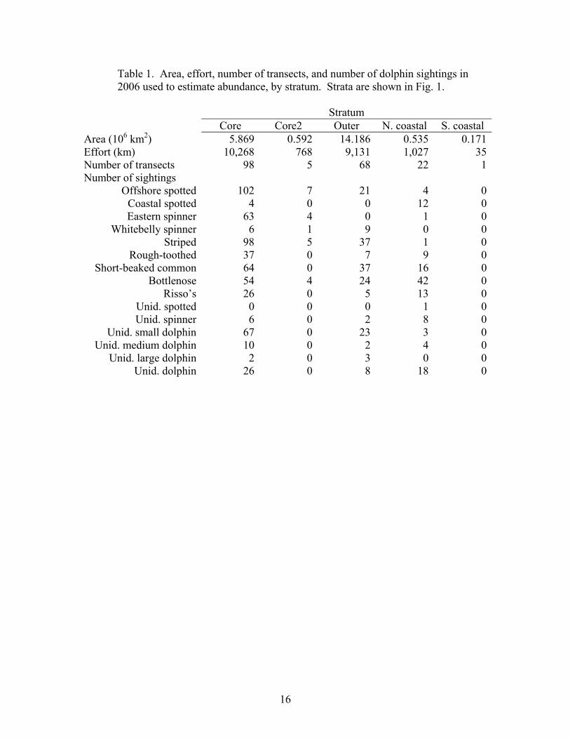
Table 1. Area, effort, number of transects, and number of dolphin sightings in 2006 used to estimate abundance, by stratum. Strata are shown in Fig. 1.

Stratum Core Core2 Outer N. coastal S. coastal Area (106 km2) 5.869 0.592 14.186 0.535 0.171Effort (km) 10,268 768 9,131 1,027 35Number of transects 98 5 68 22 1Number of sightings

Offshore spotted 102 7 21 4 0Coastal spotted 4 0 0 12 0Eastern spinner 63 4 0 1 0

Whitebelly spinner 6 1 9 0 0Striped 98 5 37 1 0

Rough-toothed 37 0 7 9 0Short-beaked common 64 0 37 16 0

Bottlenose 54 4 24 42 0Risso’s 26 0 5 13 0

Unid. spotted 0 0 0 1 0Unid. spinner 6 0 2 8 0

Unid. small dolphin 67 0 23 3 0Unid. medium dolphin 10 0 2 4 0

Unid. large dolphin 2 0 3 0 0Unid. dolphin 26 0 8 18 0

17

Table 2. Models for estimation of detection probability in 2006. All models included perpendicular distance (pd), plus covariates indicated. For each species, Model 1 is the model with lowest AIC. Additional models are shown if the AIC difference from Model 1 is less than 2.0. School size = total size of dolphin school, Beaufort = Beaufort sea state, time = local time of day. “pd only” indicates a model with perpendicular distance only (no covariates). Models for striped dolphins included a fourth model with swell height, and models for unidentified dolphins included two additional models with swell height and Beaufort, not shown here.

_Model 1_ ____Model 2____ ____Model 3____ Dolphin species covariate(s) covariate(s) ΔAIC covariate(s) ΔAIC

Spotted school size pd only 1.01

Spinner school size pd only 0.94

Striped pd only school size 0.72 time 1.88

Rough-toothed school size

Short-beaked common pd only school size 0.99 time 1.77

Bottlenose school size school size + Beaufort 1.38

Risso’s pd only school size 0.55

Unidentified pd only time 0.23 school size 0.96

18

Table 3. 2006 estimates of abundance, pooled components of abundance, and measures of their precision. N = abundance, f (0) = value of probability density function of detection at zero perpendicular distance in km-1, E (s) = expected school size, 100*n/L = encounter rate in sightings per 100 km, % pro = percentage of abundance estimate contributed by unidentified sightings, SE = standard error, CV = coefficient of variation expressed as a percentage, and lwr95 and upr95 = limits of 95% confidence interval.

Species / stock Estimate SE CV lwr95 upr95NE offshore spotted N 857884 197176 22.5 551852 1274019 f (0) 0.255 0.016 6.2 0.237 0.300 E (s) 118.2 20.0 17.3 85.8 149.9 100*n/L 0.861 0.128 14.9 0.621 1.115 % pro 2.49 2.92 103.0 0.04 10.29W/S offshore spotted N 439208 129197 28.8 227055 724675 f (0) 0.254 0.016 6.2 0.237 0.298 E (s) 114.9 16.4 14.6 87.0 141.7 100*n/L 1.258 0.162 12.9 0.960 1.582 % pro 0.13 0.19 146.3 0.02 0.50Coastal spotted N 278155 162886 59.0 31150 656534 f (0) 0.262 0.039 13.8 0.244 0.396 E (s) 223.4 130.2 61.1 24.9 539.9 100*n/L 0.080 0.023 29.1 0.037 0.128 % pro 7.37 9.35 107.7 0.40 32.78Eastern spinner N 1062879 280277 25.7 607428 1727235 f (0) 0.255 0.019 7.3 0.228 0.299 E (s) 196.3 29.1 14.9 138.9 253.3 100*n/L 0.305 0.056 18.1 0.202 0.416 % pro 8.73 7.29 80.0 0.35 26.16Whitebelly spinner N 734837 447764 60.8 154246 1802469 f (0) 0.257 0.019 7.3 0.228 0.300 E (s) 264.2 128.6 49.3 92.7 591.1 100*n/L 0.075 0.021 28.7 0.037 0.121 % pro 3.13 4.60 98.8 0.22 17.64Striped N 964362 201255 20.7 616898 1404055 f (0) 0.282 0.021 7.4 0.251 0.331 E (s) 54.8 6.3 11.8 42.1 66.8 100*n/L 0.633 0.097 15.2 0.464 0.843 % pro 0.90 1.32 119.4 0.05 4.68Rough-toothed N 107633 22908 21.6 66891 153970 f (0) 0.487 0.055 11.4 0.384 0.601 E (s) 12.2 1.6 13.4 9.3 15.6 100*n/L 0.249 0.043 17.1 0.174 0.335 % pro 1.47 1.92 110.7 0.12 6.96Short-beaked common N 3127203 835650 26.4 1620370 4876096 f (0) 0.275 0.019 6.7 0.245 0.314 E (s) 258.5 34.7 13.8 185.7 320.9 100*n/L 0.521 0.099 18.9 0.337 0.731 % pro 1.14 1.47 108.8 0.12 5.36Bottlenose N 335834 68709 19.7 231636 495304 f (0) 0.330 0.025 7.5 0.289 0.390 E (s) 23.0 3.5 14.9 17.6 31.0 100*n/L 0.577 0.079 13.6 0.434 0.735 % pro 1.15 1.29 95.5 0.16 5.10Risso’s N 110457 41355 34.8 52510 209008 f (0) 0.364 0.052 13.9 0.284 0.482 E (s) 22.3 6.1 25.8 13.5 37.8 100*n/L 0.202 0.057 28.0 0.104 0.321 % pro 1.46 1.70 99.2 0.11 6.06

19


Species / stock Estimate SE CV lwr95 upr95NE offshore spotted N 822157 127087 15.7 579926 1075088 f (0) 0.278 0.040 13.9 0.248 0.405 E (s) 91.8 12.1 13.5 59.0 108.8 100*n/L 0.909 0.106 11.8 0.697 1.100 % pro 4.49 2.71 52.8 1.19 12.06W/S offshore spotted N 758985 201434 26.5 408918 1162696 f (0) 0.277 0.039 13.5 0.248 0.397 E (s) 92.1 10.1 11.2 67.6 107.8 100*n/L 1.438 0.163 11.4 1.147 1.782 % pro 2.35 1.02 39.6 1.14 5.21Coastal spotted N 161596 46943 30.8 65979 257914 f (0) 0.329 0.052 16.1 0.261 0.449 E (s) 53.2 15.5 27.3 32.5 91.8 100*n/L 0.343 0.103 32.6 0.097 0.497 % pro 12.41 6.96 51.9 2.64 31.20Eastern spinner N 673943 147914 22.1 408922 977001 f (0) 0.251 0.039 15.4 0.189 0.359 E (s) 123.5 18.0 14.5 93.1 163.7 100*n/L 0.306 0.053 17.9 0.195 0.406 % pro 2.68 8.31 158.2 0.70 33.32Whitebelly spinner N 531496 229556 43.2 170363 1022845 f (0) 0.259 0.040 15.4 0.190 0.358 E (s) 86.2 17.6 19.6 61.5 132.4 100*n/L 0.136 0.049 39.3 0.030 0.212 % pro 5.90 15.46 145.3 1.55 63.81Striped N 1617012 283949 19.7 924869 2025765 f (0) 0.357 0.036 10.7 0.280 0.422 E (s) 54.0 5.9 11.1 39.3 63.3 100*n/L 0.682 0.108 16.3 0.454 0.874 % pro 1.93 0.82 38.7 1.03 4.30Rough-toothed N 47593 16484 31.0 27218 92670 f (0) 0.432 0.103 21.4 0.365 0.764 E (s) 8.9 0.9 10.2 7.4 10.9 100*n/L 0.157 0.030 19.8 0.099 0.215 % pro 1.43 0.75 46.1 0.72 3.46Short-beaked common N 1197168 472773 35.5 709369 2669497 f (0) 0.319 0.036 11.6 0.249 0.382 E (s) 129.6 27.8 19.1 107.7 222.4 100*n/L 0.331 0.058 17.4 0.233 0.451 % pro 1.66 1.84 82.8 0.90 8.13Bottlenose N 312225 87168 26.8 188168 509506 f (0) 0.324 0.038 11.3 0.293 0.435 E (s) 40.6 16.8 43.2 17.9 80.7 100*n/L 0.583 0.083 14.0 0.440 0.765 % pro 0.94 0.65 55.0 0.43 3.06Risso’s N 81474 20304 24.8 48140 122422 f (0) 0.365 0.044 11.8 0.287 0.459 E (s) 18.6 3.9 20.9 11.8 26.6

100*n/L 0.203 0.044 21.6 0.131 0.295% pro 1.37 0.62 40.0 0.72 3.18

20



21



100*n/L 0.168 0.042 24.9 0.097 0.259% pro 1.83 0.60 33.5 0.89 3.15

22


Species / stock Estimate SE CV lwr95 upr95NE offshore spotted N 689410 95005 13.5 525396 902631 f (0) 0.378 0.020 5.3 0.339 0.419 E (s) 63.9 6.1 9.3 53.7 77.9 100*n/L 0.787 0.092 11.8 0.607 0.967 % pro 9.72 3.50 37.0 4.14 17.47W/S offshore spotted N 765437 229771 29.6 390996 1277560 f (0) 0.373 0.020 5.2 0.338 0.415 E (s) 72.9 6.7 9.0 61.7 87.9 100*n/L 1.315 0.140 10.7 1.050 1.600 % pro 3.33 1.67 51.1 1.07 7.31Coastal spotted N 125248 38629 32.9 52678 199845 f (0) 0.454 0.049 11.7 0.343 0.503 E (s) 57.5 19.4 31.5 31.8 111.0 100*n/L 0.122 0.029 23.8 0.071 0.188 % pro 25.05 12.32 51.1 4.34 50.49Eastern spinner N 545213 132873 23.6 341864 854979 f (0) 0.338 0.024 7.2 0.294 0.389 E (s) 111.7 14.5 12.6 89.8 147.4 100*n/L 0.230 0.037 16.1 0.163 0.309 % pro 4.63 1.97 43.8 2.13 9.56Whitebelly spinner N 271442 103317 36.5 102823 509931 f (0) 0.338 0.024 7.2 0.295 0.388 E (s) 103.3 26.2 24.3 59.5 160.7 100*n/L 0.039 0.011 27.1 0.020 0.061 % pro 12.62 9.07 74.3 1.47 32.61Striped N 1066521 151115 14.1 796923 1379690 f (0) 0.408 0.024 5.8 0.367 0.460 E (s) 41.8 3.1 7.4 36.5 48.6 100*n/L 0.490 0.047 9.5 0.402 0.578 % pro 3.11 1.33 43.6 1.31 6.36Rough-toothed N 68274 19300 28.1 35618 110086 f (0) 0.698 0.069 9.7 0.585 0.893 E (s) 9.4 1.2 13.2 7.1 12.0 100*n/L 0.115 0.018 15.5 0.082 0.152 % pro 2.71 0.93 34.9 1.43 5.06Short-beaked common N 2277456 580256 25.5 1258256 3543480 f (0) 0.352 0.025 7.2 0.303 0.402 E (s) 194.8 39.2 19.9 128.9 280.0 100*n/L 0.319 0.043 13.6 0.240 0.408 % pro 5.93 2.75 46.9 2.05 12.78Bottlenose N 327166 76444 23.2 202889 495622 f (0) 0.417 0.023 5.5 0.379 0.467 E (s) 20.1 2.6 13.2 15.2 25.3 100*n/L 0.657 0.075 11.4 0.524 0.816 % pro 2.27 0.67 30.4 1.30 3.81Risso’s N 64962 14567 20.8 44235 101914 f (0) 0.372 0.051 12.4 0.331 0.523

E (s) 17.1 4.2 25.2 10.3 26.1100*n/L 0.199 0.035 17.6 0.133 0.271% pro 2.34 0.63 26.7 1.43 4.04

23


Species / stock Estimate SE CV lwr95 upr95NE offshore spotted N 755112 294936 39.1 321828 1459104 f (0) 0.254 0.020 8.0 0.218 0.303 E (s) 112.0 36.4 33.2 55.6 192.3 100*n/L 0.660 0.106 16.1 0.458 0.874 % pro 11.44 7.76 67.7 2.40 29.25W/S offshore spotted N 533076 123379 23.1 314099 797611 f (0) 0.252 0.020 7.7 0.217 0.299 E (s) 136.8 27.4 20.6 86.7 193.9 100*n/L 0.622 0.075 12.0 0.480 0.781 % pro 35.32 10.35 28.0 17.32 58.03Coastal spotted N 3350 3424 107.2 0 11098 f (0) 0.262 0.041 14.9 0.223 0.397 E (s) 17.9 6.0 33.2 9.0 31.5 100*n/L 0.006 0.005 95.0 0.000 0.016 % pro 11.89 9.16 60.8 2.22 35.22Eastern spinner N 460952 158402 33.6 218201 852120 f (0) 0.300 0.032 10.6 0.250 0.374 E (s) 102.7 22.7 22.2 66.3 150.9 100*n/L 0.145 0.027 18.8 0.095 0.205 % pro 11.21 7.47 66.0 2.49 29.80Whitebelly spinner N 422259 236502 54.0 116459 992160 f (0) 0.301 0.039 12.6 0.254 0.417 E (s) 179.0 75 42.5 78.1 357.7 100*n/L 0.068 0.018 26.4 0.034 0.104 % pro 5.48 2.59 46.4 2.21 11.56Striped N 1053945 179309 16.7 755738 1464656 f (0) 0.347 0.025 7.2 0.305 0.403 E (s) 62.7 6.6 10.5 50.2 76.9 100*n/L 0.462 0.047 10.1 0.371 0.555 % pro 7.49 3.27 42.0 3.28 15.95Rough-toothed N 122454 52405 42.7 46080 238586 f (0) 0.563 0.054 9.4 0.485 0.688 E (s) 25.1 9.1 36.6 12.3 46.6 100*n/L 0.084 0.018 21.0 0.051 0.119 % pro 7.88 5.28 60.8 2.57 21.36Short-beaked common N 1148256 336943 28.9 573654 1886923 f (0) 0.318 0.034 10.7 0.260 0.392 E (s) 313.3 65.8 20.7 212.9 467.4 100*n/L 0.100 0.027 26.9 0.053 0.159 % pro 12.92 6.40 48.5 3.51 28.37Bottlenose N 190351 56326 28.3 108761 324815 f (0) 0.340 0.044 12.6 0.277 0.447 E (s) 25.2 4.4 17.2 17.7 34.3 100*n/L 0.216 0.032 14.8 0.157 0.282 % pro 8.50 4.44 49.1 3.25 19.04Risso’s N 120165 164392 131.8 41011 419940 f (0) 0.570 0.056 9.6 0.488 0.710 E (s) 19.4 23.7 120.0 9.4 60.3

100*n/L 0.100 0.025 24.8 0.057 0.153% pro 5.58 3.47 56.7 1.60 14.47

24


Species / stock Estimate SE CV lwr95 upr95NE offshore spotted N 1012176 246687 23.5 641315 1624213 f (0) 0.270 0.017 6.1 0.249 0.313 E (s) 152.4 32.7 21.1 106.1 227.9 100*n/L 0.661 0.102 15.4 0.467 0.872 % pro 11.12 4.77 43.5 3.47 21.57W/S offshore spotted N 1234593 403802 30.9 699684 2219923 f (0) 0.288 0.017 5.8 0.269 0.337 E (s) 163.5 24.9 15.1 124.2 218.5 100*n/L 0.894 0.109 12.2 0.684 1.120 % pro 19.06 10.06 52.6 3.50 41.05Coastal spotted N - - - - - f (0) - - - - - E (s) - - - - - 100*n/L - - - - - % pro - - - - - Eastern spinner N 617298 195391 30.9 314479 1062500 f (0) 0.284 0.021 7.3 0.247 0.327 E (s) 118.6 29.6 24.4 73.8 185.2 100*n/L 0.242 0.040 16.6 0.166 0.329 % pro 4.52 2.83 69.5 1.25 11.53Whitebelly spinner N 952381 441688 42.9 333384 2029577 f (0) 0.294 0.031 10.0 0.268 0.388 E (s) 208.1 47.9 22.8 127.6 313.3 100*n/L 0.103 0.022 21.6 0.063 0.149 % pro 0.82 0.94 112.1 0.25 2.70Striped N 1299832 306296 21.1 963433 2126277 f (0) 0.353 0.035 9.2 0.321 0.452 E (s) 54.9 6.2 11.0 45.1 68.6 100*n/L 0.673 0.064 9.5 0.557 0.806 % pro 2.09 1.41 70.5 0.72 5.42Rough-toothed N 59032 24426 41.6 25300 120001 f (0) 0.495 0.069 13.6 0.394 0.663 E (s) 13.9 5.1 37.4 8.4 28.6 100*n/L 0.103 0.023 22.2 0.061 0.152 % pro 3.99 2.35 62.9 1.32 10.46Short-beaked common N 2330910 799899 34.2 1086694 4109733 f (0) 0.328 0.040 12.2 0.254 0.410 E (s) 400.4 113.5 28.3 243.5 629.3 100*n/L 0.157 0.034 21.4 0.099 0.227 % pro 12.43 6.84 52.7 2.44 29.21Bottlenose N 141091 44770 30.5 73102 251281 f (0) 0.418 0.054 13.4 0.299 0.508 E (s) 17.3 4.2 23.1 11.4 28.2 100*n/L 0.200 0.036 17.6 0.139 0.274 % pro 2.54 1.76 71.9 0.76 6.60Risso’s N 78596 30476 37.5 38772 139034 f (0) 0.495 0.069 13.6 0.394 0.663

E (s) 13.4 3.7 27.9 7.6 21.0100*n/L 0.135 0.027 20.0 0.088 0.194% pro 3.36 2.26 71.5 0.99 8.45

25


Species / stock Estimate SE CV lwr95 upr95NE offshore spotted N 906369 213612 23.3 528342 1354159 f (0) 0.331 0.024 7.3 0.290 0.383 E (s) 145.1 19.5 13.4 107.0 186.2 100*n/L 0.552 0.096 17.4 0.373 0.751 % pro 1.44 0.77 53.1 0.60 3.19W/S offshore spotted N 1161047 684108 57.3 416915 2630931 f (0) 0.331 0.025 7.4 0.290 0.386 E (s) 152.9 29.2 19.0 115.5 214.4 100*n/L 0.703 0.100 14.3 0.509 0.909 % pro 12.87 9.31 62.1 2.49 38.69Coastal spotted N - - - - - f (0) - - - - - E (s) - - - - - 100*n/L - - - - - % pro - - - - - Eastern spinner N 679538 198460 30.2 303807 1094261 f (0) 0.359 0.030 8.4 0.305 0.421 E (s) 160.5 33.5 21.2 100.0 235.1 100*n/L 0.155 0.038 24.8 0.088 0.238 % pro 1.23 0.66 51.8 0.50 2.52Whitebelly spinner N 875437 250535 29.3 417373 1354965 f (0) 0.359 0.030 8.4 0.308 0.422 E (s) 101.4 24.5 24.5 59.1 154.5 100*n/L 0.168 0.034 20.3 0.104 0.238 % pro 2.43 1.14 44.0 1.05 5.16Striped N 1544721 234479 15.0 1135040 2013991 f (0) 0.336 0.019 5.8 0.301 0.377 E (s) 62.2 3.8 6.1 55.1 70.1 100*n/L 0.760 0.075 9.9 0.616 0.915 % pro 2.25 0.89 38.4 1.18 4.40Rough-toothed N 110349 35919 32.7 50173 191045 f (0) 0.615 0.060 9.8 0.519 0.749 E (s) 12.6 4.3 32.7 7.3 24.1 100*n/L 0.147 0.047 32.0 0.069 0.250 % pro 1.58 0.79 45.9 0.67 3.76Short-beaked common N 3630548 2096690 57.2 1338894 8633349 f (0) 0.284 0.030 10.5 0.229 0.356 E (s) 426.7 102 23.8 247.8 639.8 100*n/L 0.210 0.047 22.5 0.127 0.308 % pro 38.03 22.49 78.8 1.11 73.57Bottlenose N 167560 61383 35.2 79029 304083 f (0) 0.354 0.043 11.8 0.291 0.461 E (s) 23.7 6.9 28.9 13.5 36.6 100*n/L 0.231 0.041 17.9 0.153 0.312 % pro 1.36 0.83 60.6 0.51 3.11Risso’s N 128104 66660 49.9 58939 247266 f (0) 0.620 0.059 9.4 0.530 0.760 E (s) 11.4 4.9 42.0 7.3 21.1

100*n/L 0.172 0.033 19.1 0.114 0.240% pro 1.44 0.74 48.2 0.52 3.38

26



100*n/L 0.189 0.031 16.4 0.130 0.250% pro 4.18 1.96 43.5 2.35 9.05

27



28

Table 13. Estimates of exponential rate of change r, with lower and upper limits of the 95% confidence interval on the estimate, for 10 ETP dolphin stocks for two time periods: 1986-2006 and 1998-2006.

1986 - 2006 1998 – 2006 Species / stock r lwr95 upr95 r lwr95 upr95 NE offshore spotted 0.010 -0.014 0.034 0.035 -0.002 0.071W/S offshore spotted -0.023 -0.058 0.013 -0.080 -0.189 0.028Coastal spotted 0.104 0.004 0.204 0.077 -0.091 0.245Eastern spinner 0.019 -0.013 0.051 0.092 -0.017 0.202Whitebelly spinner -0.005 -0.054 0.043 0.062 -0.302 0.425Striped -0.004 -0.028 0.020 0.012 -0.095 0.119Rough-toothed 0.026 -0.022 0.074 0.081 -0.071 0.232Short-beaked common 0.047 -0.012 0.107 -0.006 -0.221 0.208Bottlenose 0.040 0.020 0.060 -0.004 -0.033 0.024Risso's 0.011 -0.017 0.040 0.039 -0.112 0.189

29

160°W 145°W 130°W 115°W 100°W 85°W 70°W

160°W 145°W 130°W 115°W 100°W 85°W 70°W

20°S

5°S

10°N

25°N

20°S

5°S

10°N

25°N

Longitude

Latit

ude

CORE

CO

RE

2

OUTER

NORTH COASTALSO

UTH COASTAL

Fig. 1. Strata for the STAR06 cruise.

160°W 145°W 130°W 115°W 100°W 85°W 70°W

160°W 145°W 130°W 115°W 100°W 85°W 70°W

15°S

0°

15°N

30°N

15°S

0°

15°N

30°N

Fig. 2: Line-transect effort (broken dark lines) and stratum boundaries (solid gray lines) for the STAR06 cruise.

30

1986 1987 1988 1989 1990 1998 1999 2000 2003 2006

Distance on effortNumber of transects

DIS

TAN

CE

ON

EFF

OR

T (1

000

km)

010

2030

40

010

020

030

0

NU

MB

ER

OF

TR

AN

SE

CTS

(da

ys o

n ef

fort)

Fig. 3: Two measures of survey effort in the ETP by year.

31

160°W 145°W 130°W 115°W 100°W 85°W 70°W

160°W 145°W 130°W 115°W 100°W 85°W 70°W

15°S

0°

15°N

30°N

15°S

0°

15°N

30°N

Stenella attenuata (offshore)Stenella attenuata graffmaniStenella attenuata (unid. subsp.)

Fig. 4: Spotted dolphin sightings during STAR06. Gray lines are stratum boundaries and survey effort.

160°W 145°W 130°W 115°W 100°W 85°W 70°W

160°W 145°W 130°W 115°W 100°W 85°W 70°W

15°S

0°

15°N

30°N

15°S

0°

15°N

30°N

Stenella longirostris orientalisStenella longirostris (whitebelly)Stenella longirostris (southwestern)Stenella longirostris (unid. subsp.)

Fig. 5: Spinner dolphin sightings during STAR06. Gray lines are stratum boundaries and survey effort.

32

160°W 145°W 130°W 115°W 100°W 85°W 70°W

160°W 145°W 130°W 115°W 100°W 85°W 70°W

15°S

0°

15°N

30°N

15°S

0°

15°N

30°N

Stenella coeruleoalba

Fig. 6: Striped dolphin sightings during STAR06. Gray lines are stratum boundaries and survey effort.

160°W 145°W 130°W 115°W 100°W 85°W 70°W

160°W 145°W 130°W 115°W 100°W 85°W 70°W

15°S

0°

15°N

30°N

15°S

0°

15°N

30°N

Steno bredanensis

Fig. 7: Rough-toothed dolphin sightings during STAR06. Gray lines are stratum boundaries and survey effort.

33

160°W 145°W 130°W 115°W 100°W 85°W 70°W

160°W 145°W 130°W 115°W 100°W 85°W 70°W

15°S

0°

15°N

30°N

15°S

0°

15°N

30°N

Delphinus delphis

Fig. 8: Common dolphin sightings during STAR06. Gray lines are stratum boundaries and survey effort.

160°W 145°W 130°W 115°W 100°W 85°W 70°W

160°W 145°W 130°W 115°W 100°W 85°W 70°W

15°S

0°

15°N

30°N

15°S

0°

15°N

30°N

Tursiops truncatus

Fig. 9: Bottlenose dolphin sightings during STAR06. Gray lines are stratum boundaries and survey effort.

34

160°W 145°W 130°W 115°W 100°W 85°W 70°W

160°W 145°W 130°W 115°W 100°W 85°W 70°W

15°S

0°

15°N

30°N

15°S

0°

15°N

30°N

Grampus griseus

Fig. 10: Risso’s dolphin sightings during STAR06. Gray lines are stratum boundaries and survey effort.

160°W 145°W 130°W 115°W 100°W 85°W 70°W

160°W 145°W 130°W 115°W 100°W 85°W 70°W

15°S

0°

15°N

30°N

15°S

0°

15°N

30°N

unid. dolphinunid. small delphinidunid. medium delphinidunid. large delphinid

Fig. 11: Unidentified dolphin sightings during STAR06. Gray lines are stratum boundaries and survey effort.

35

PERPENDICULAR DISTANCE (km)

PRO

BABI

LITY

DEN

SITY

0 1 2 3 4 5

00.

10.

20.

3

Spotted


PRO

BABI

LITY

DEN

SITY

0 1 2 3 4 5

00.

10.

20.

3 Spinner


PRO

BABI

LITY

DEN

SITY

0 1 2 3 4 5

00.

10.

20.

3

Striped


PRO

BABI

LITY

DEN

SITY

0 1 2 3 4 50

0.1

0.2

0.3

0.4

0.5

Rough-toothed


PRO

BABI

LITY

DEN

SITY

0 1 2 3 4 5

00.

10.

20.

3 Short-beaked common


PRO

BABI

LITY

DEN

SITY

0 1 2 3 4 5

00.

10.

20.

30.

40.

5 Bottlenose


PRO

BABI

LITY

DEN

SITY

0 1 2 3 4 5

00.

10.

30.

50.

7 Risso's


PRO

BABI

LITY

DEN

SITY

0 1 2 3 4 5

00.

10.

20.

30.

4 unidentified

Fig. 12: Histograms of perpendicular distances to sightings of dolphins of different species during STAR06, with half-normal detection functions.

36

1986 1987 1988 1989 1990 1998 1999 2000 2003 2006

2.0

2.5

3.0

3.5

4.0

4.5

5.0

Northeastern offshore spottedE

FFE

CTI

VE

STR

IP W

IDTH

(km

)

1986 1987 1988 1989 1990 1998 1999 2000 2003 2006

2.0

2.5

3.0

3.5

4.0

4.5

5.0

Eastern spinner

EFF

EC

TIV

E S

TRIP

WID

TH (

km)

Fig. 13: Bootstrap distributions of pooled effective strip width [1/ ˆ (0)f , eq. 2] by year for northeastern offshore spotted and eastern spinner dolphins. Dark horizontal lines show medians, open boxes first and third quartiles, and dashed vertical lines the range of values within twice the interquartile range.

1987 1988 1989 1990 1992 1993 1998 1999 2000 2003 2006

OB

SE

RV

ER

ES

TIM

ATE

/ P

HO

TO C

OU

NT

0.25

0.5

12

4

n = 244 268 200 205 273 295 183 210 165 200 232

Fig. 14: Distributions of the ratio of an observer’s best estimate of school size to the count of dolphins in an aerial photograph of the school, by year. Sample size is given along the top. Note the logarithmic scale, and that calibration photographs were carried out in 1992 and 1993 although abundance estimates are not available in those years. The solid horizontal line indicates estimates equal to the photo count (a ratio of 1.0). The dotted horizontal line is the overall median ratio of 0.71.

37

010

020

030

040

0

SC

HO

OL

SIZ

E

BottlenoseCoastalspotted

Easternspinner

Offshorespotted Risso's

Short-beakedcommon Steno Striped

Whitebellyspinner

*

**

**

*

**

*

Fig. 15: Distributions of school sizes observed on STAR06 by stock. Means (*), medians (dark horizontal lines), 95% confidence intervals on the medians (hatched boxes), interquartile ranges (open boxes), standard spans (dashed lines), and outliers (circles) are shown for sightings used in abundance estimation. Some outliers are not shown.

1986 1987 1988 1989 1990 1998 1999 2000 2003 2006

5010

015

020

025

030

0

Northeastern offshore spotted

SC

HO

OL

SIZ

E

1986 1987 1988 1989 1990 1998 1999 2000 2003 2006

5010

015

020

025

030

0

Eastern spinner

SC

HO

OL

SIZ

E

Fig. 16: Bootstrap distributions of pooled expected school size [ E( )s , eq. 3] by year for northeastern offshore spotted and eastern spinner dolphins. Dark horizontal lines show medians, open boxes first and third quartiles, and dashed vertical lines the range of values within twice the interquartile range.

38

1986 1987 1988 1989 1990 1998 1999 2000 2003 2006

0.4

0.6

0.8

1.0

1.2


EN

CO

UN

TER

RA

TE (

scho

ols/

100k

m)

1986 1987 1988 1989 1990 1998 1999 2000 2003 2006

0.1

0.2

0.3

0.4

Eastern spinner

EN

CO

UN

TER

RA

TE (

scho

ols/

100k

m)

Fig. 17: Bootstrap distributions of pooled encounter rate (schools/100km, 100n/L, eq. 4) by year for northeastern offshore spotted and eastern spinner dolphins. Dark horizontal lines show medians, open boxes first and third quartiles, and dashed vertical lines the range of values within twice the interquartile range. Note the different ordinate scales.

39

050

010

0015

00

ABU

ND

ANC

E (i

n th

ousa

nds)

1985 1990 1995 2000 2005


050

015

0025

00

ABU

ND

ANC

E (i

n th

ousa

nds)

1985 1990 1995 2000 2005

Western/southern offshore spotted

010

030

050

0

ABU

ND

ANC

E (i

n th

ousa

nds)

1985 1990 1995 2000 2005

Coastal spotted

050

010

0015

00

ABU

ND

ANC

E (i

n th

ousa

nds)

1985 1990 1995 2000 2005

Eastern spinner

050

010

0015

0020

00

ABU

ND

ANC

E (i

n th

ousa

nds)

1985 1990 1995 2000 2005

Whitebelly spinner0

500

1000

1500

2000

ABU

ND

ANC

E (i

n th

ousa

nds)

1985 1990 1995 2000 2005

Striped

050

100

150

200

ABU

ND

ANC

E (i

n th

ousa

nds)

1985 1990 1995 2000 2005

Rough-toothed

020

0040

0060

0080

00

ABU

ND

ANC

E (i

n th

ousa

nds)

1985 1990 1995 2000 2005

Short-beaked common

010

030

050

0

ABU

ND

ANC

E (i

n th

ousa

nds)

1985 1990 1995 2000 2005

Bottlenose

010

020

030

040

0

ABU

ND

ANC

E (i

n th

ousa

nds)

1985 1990 1995 2000 2005

Risso's

Fig 18: Estimates of abundance for 10 dolphin stocks for 10 surveys between 1986 and 2006. Vertical lines show 95% confidence intervals on the point estimates based on a bootstrap procedure. Solid lines show fit of a model of exponential change from 1986-2006, dashed lines from 1998-2006. Statistics of model fit are summarized in Table 13.

RECENT TECHNICAL MEMORANDUMSCopies of this and other NOAA Technical Memorandums are available from the National Technical Information Service, 5285 Port Royal Road, Springfield, VA 22167. Paper copies vary in price. Microfiche copies cost $9.00. Recent issues of NOAA Technical Memorandums from the NMFS Southwest Fisheries Science Center are listed below:

NOAA-TM-NMFS-SWFSC-412 Updated estimates of mortality and injury of cetaceans in the Hawaii- based longline fishery, 1994-2005. K.A. FORNEY and D.R. KOBAYASHI (November 2007)

413 Assessment of the Pacific sardine resource in 2007 for U.S. Management in 2008. K.T. HILL, E. DORVAL, N.C.H. LO, B.J. MACEWICZ, C. SHOW and R. FELIX-URAGA (December 2007

414 U.S. Pacific marine mammal stock assessments: 2007. J.V. CARRETTA, K.A. FORNEY, M.S. LOWRY, J. BARLOW, J. BAKER, B. HANSON, and M.M. MUTO (December 2007)

415 California current ecosystem survey 2006 acoustic cruise reports for NOAA FSV Oscar Dyson and NOAA FRV David Starr Jordan G.R. CUTTER, JR., Editor and D.A. DEMER (January 2008)

416 An assessment of the accuracy and precision of localization of a stationary sound source using a two-element towed hydrophone array. S. RANKIN, J. BARLOW, and J. OSWALD (January 2008)

417 A guide to consturcting hydrophones and hydrophone arrays for monitoring marine mammal vocalizations. J. BARLOW, S. RANKIN, and S. DAWSON (February 2008)

418 Diet of the striped dolphin, Stenella coeruleoalba, in the eastern tropical Pacific ocean. W.F. PERRIN, K.M. ROBERTSON, and W.A. WALKER (March 2008)

419 Report of a hydrographic survey of Clipperton Ridge conducted aboard the David Starr Jordan during the Stenella abundance research cruise 2006. C. HALL, K.W. ROBERTS, S.M. FINNEY, W.P. MOWITT, D. GOTHAN, and L.T. BALLANCE (March 2008)

420 Marine mammal data collected during the Pacific islands cetacean and ecosystem assessment survey (PICEAS) conducted aboard the NOAA ship McArthur II, July - November 2005. J. BARLOW, S. RANKIN, A. JACKSON, and A. HENRY (March 2008)

421 Marine mammal data collected during a survey in the eastern tropical Pacific ocean aboard NOAA ships David Starr Jordan and McArthur II, July 28 - December 7, 2006. A. JACKSON, T. GERRODETTE, S. CHIVERS, M. LYNN, S. RANKIN, and S. MESNICK (April 2008)