NOAA Technical Memorandum ERL GLERL-37

AN EQUILIBRIUM MODEL FOR THE PARTITIONING OF SYNTHETIC

ORGANIC COMPOUNDS INCORPORATING FIRST-ORDER DECOMPOSITION

B. J. EadieM. J. McCormickC. RiceP. LeVonM. Simmons

Great Lakes Environmental Research LaboratoryAnn Arbor, MichiganOctober 1981

IJEPARTMENT OF COMMERCENATIONAL OCEANIC ANDATMOSPHERIC ADMINISTRATION

John V. Byrne.Administrator

Environmental ResearchLaboratories

George H. LudwigDirector

NOTICE

Mention of a conaercial company or product does not constitutean endorsement by NOM Environmental Research Laboratories.Use for publicity or advertising purposes of information fromthis publication concerning proprietary products or the testsof such products is not authorized.

CONTENTS

Abstract

1. INTRODUCTION

2. THE EQUILIBRIUM MODEL

3. INCORPORATING DECOMPOSITION

4. DEFINING THE ECOSYSTEM

5. THE MODEL'S OPERATION

5.1 Model Runs

5.2 The Model Applied to DDT

5.3 The Model Applied to PCB's

5.4 Microbial Degradation

6. RESULTS

7. ACKNOWLEDGHENTS

8. REFERENCES

9. Appendix--PROGRAM OUTPUT

Page

1

1

1

4

4

5

6

6

a

12

16

22

23

25

iii

FIGURES

Page

1.

2.

3.

4.

5.

6.

7.

8.

Model output of DDT concentrations in fish, biota, and sedi-ments.

DDT concentrations.

DDT loss rates.

Isomeric composition of commercially available Aroclors".

a) PCB mixtures in biota using the low rates in table 2.b) PCB mixtures in sediments for the same run.

a) PCB mixtures in biota using the high rates in table 2.b) PCB mixtures in sediments for the same run.

Total PCB's in Lake Michigan fish.

PCB loss rates from the summer scenario (figure 6). a) Aroclor"1242, b) Aroclor@ 1254, and c) Aroclor" 1260.

'7

9

9

10

17

18

20

21

iv

TABLES

1. Input parameters for DDT model.

2. Input parameters for PCB model.

3. Laboratory microbial decomposition of PCB (per day).

Page

7

11

14

AN EQUILIBRIUM MODEL FOR THE PARTITIONING OF SYNTHETIC OfjGANICCOMPOUNDS INCORPORATING FIRST-ORDER DECOMPOSITION

B. J. Eadie, M. J. McCormick, C. Rice, P. IeVon, and M. Simmons

A simple equilibrium model incorporating several first-orderdecomposition athways has been calibrated for DDT and PCB mix-tures in a l-ms ecosystem with the characteristics of LakeMichigan. This exercise has revealed the weakness in currentlyavailable process-rate information. The model, as constructed,yields some valuable insights into the environmental pathways ofhydrophobic organic contaminants in aquatic ecosystems.

1. INTRODUCTION

A previous report (Eadie, 1981) described a model based on the con-cept of fugacity, which predicted the equilibrium distribution of hydropho-bic organic contaminants in aquatic ecosystems. This model did not containdecomposition and as such could only describe a static ecosystem. Althoughmany synthetic organic compounds are designed and used because of their sta-bility, they are subject to multiple environmental decomposition pathways,such as photolysis, biological decomposition, and chemical oxidation.These, along with physical processes, such as outflow and sediment burial,combine to remove the contaminant from an ecosystem. The obvious questionto ask of a model is how long will it be before the contaminant concentra-tion drops below a specified level.

There are several ways to address such questions; the approach basi-cally comes down to the level of detail required and the level of infor-mation available. The latter is the constraining factor in the developmentof ecosystem models. This report describes a simplified approach in whichall transformations are handled as first order with respect to contaminantconcentration and that provides useful insight into the fates of syntheticorganic compounds in well-mixed aquatic systems.

2. THE EQUILIBRIUM MODEL

The model, which is based on the fugacity concept described in detailelsewhere (Mackay, 1979; Eadie. 1981). assumes all compartments are in

*GLERL Contribution No. 266.

1

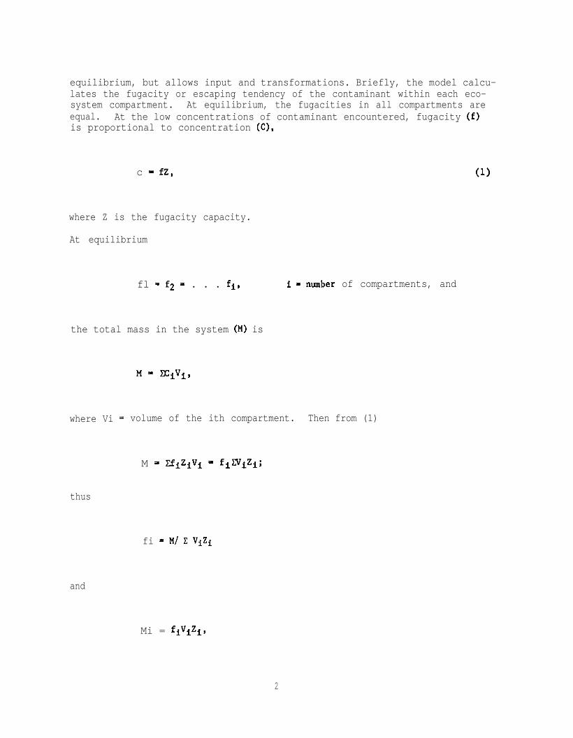
equilibrium, but allows input and transformations. Briefly, the model calcu-lates the fugacity or escaping tendency of the contaminant within each eco-system compartment. At equilibrium, the fugacities in all compartments areequal. At the low concentrations of contaminant encountered, fugacity (f)is proportional to concentration (C),

c = fZ, (1)

where Z is the fugacity capacity.

At equilibrium

fl = f2 = . . . fir i - number of compartments, and

the total mass in the system (M) is

where Vi = volume of the ith compartment. Then from (1)

M - ZfiZfVi = fiZ’JiZi;

thus

fi = Mf C ViZi

and

Mi = fiViZi,

2

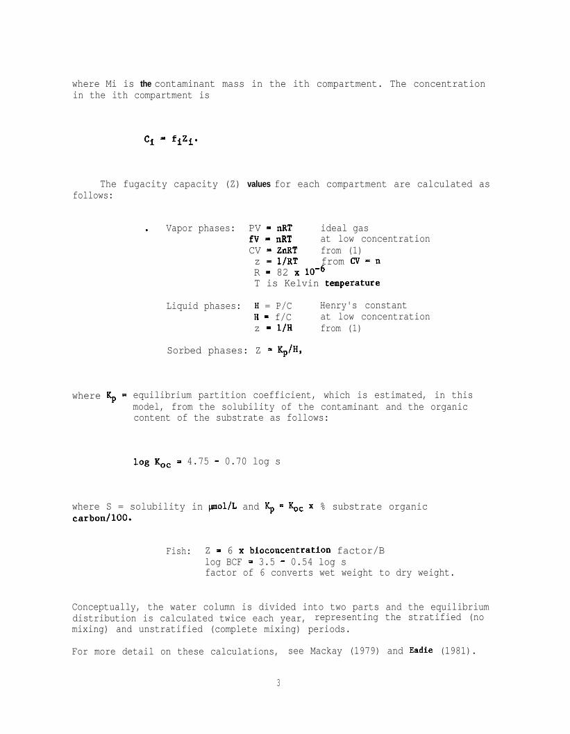
where Mi is the contaminant mass in the ith compartment. The concentrationin the ith compartment is

Cl = fiZi.

The fugacity capacity (Z) values for each compartment are calculated asfollows:

. Vapor phases: PV = nRT ideal gasfV * nRT at low concentrationCV = ZnRT from (1)z = l/RT from CV = nR = 82 x lo+T is Kelvin temperatUre

Liquid phases: H = P/C Henry's constantH = f/C at low concentrationz = l/H from (1)

Sorbed phases: Z = Kp/H,

where Kp = equilibrium partition coefficient, which is estimated, in thismodel, from the solubility of the contaminant and the organiccontent of the substrate as follows:

log Kc,, - 4.75 - 0.70 log s

where S = solubility in pmol/L and Kp = Koc x % substrate organiccarbon/lOO.

Fish: Z = 6 x bioconcentration factor/Blog BCF = 3.5 - 0.54 log sfactor of 6 converts wet weight to dry weight.

Conceptually, the water column is divided into two parts and the equilibriumdistribution is calculated twice each year, representing the stratified (nomixing) and unstratified (complete mixing) periods.

For more detail on these calculations, see Mackay (1979) and Eadie (1981).

3

3. INCOKPOBATING DECOMPOSITION

A more realistic model is constructed by including decomposition pro-cesses (photolysis, biolysis), settling, and burial in the fugacity model.All of the removal mechanisms are approximated as first-order reactions.The sum of the first-order rates for each compartment (I), period (j) is:

n

Kij - "Ki,j,k* n - number of processes.k-l

Thus the total removal rate from compartment I is

ViCi,jKi,j molfhalf year.

4. DEFINING TEE ECOSYSTEM

For the purposes of initial analyses and flexibility, the ecosystemwill represent a 1-m2, loo-m-deep basin with the biological and sedimentarycharacteristics of lake Michigan.

Ecosystem compartment

AtmosphereEpilimnionHypolimnionDetritusBiotaSedimentsFish

Volume (m3) comments

104 10 km thick25 25 m deep75 751.5 x 10-4

m deep

5 x 10-S1.5 ppm; 10% organic order

5010-2

mg/m3; 40% organic order2 x 22 x 10-7

cm mixed; 2% organic order

The semiannual time steps represent a cold, well-mixed system (temper-atures - 4°C) and a stratified condition with an epilimnion temperature of20°C and hypolimnion temperature held at 4°C. A caveat in this conceptualframework is that the sediments and hypolimnion are considered to be inequilibrium with the epilimnion and atmosphere during the stratified periodwhen it is well known that transport through the thermocline region issmall. The effect of this will be discussed later.

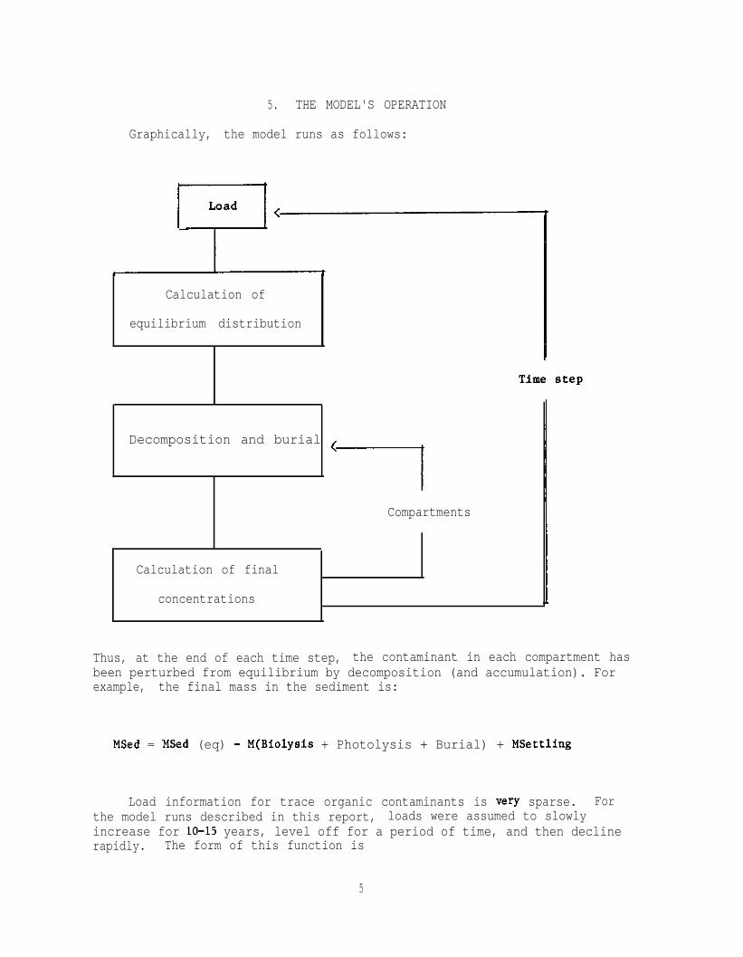
5. THE MODEL'S OPERATION

Graphically, the model runs as follows:

Calculation of

equilibrium distribution

Decomposition and burial <

./

Compartments

Calculation of final

concentrations

Thus, at the end of each time step, the contaminant in each compartment hasbeen perturbed from equilibrium by decomposition (and accumulation). Forexample, the final mass in the sediment is:

MSed = MSed (eq) - M(Biolysis + Photolysis + Burial) + MSettling

Load information for trace organic contaminants is very sparse. Forthe model runs described in this report, loads were assumed to slowlyincrease for lo-15 years, level off for a period of time, and then declinerapidly. The form of this function is

5

LOAD = t2 (Cl - c2t)

where t - time.

By adjusting cl and c2

, the loading function can be altered to conformto the limited data availa le.

Detritus settling is set at - 0.3 m/day (Chambers and Eadie, 1981);thus, one-half of the detritus mass enters the sediment each time step andan equivalent mass of sediment is buried, leaving the mixed layer constant.For this model, the detritus mass is renewed each time step, keeping allcompartment volumes constant. At the end of each time step, a mass balancecalculation is made to warn of any internal inconsistencies.

5.1 Model Runs

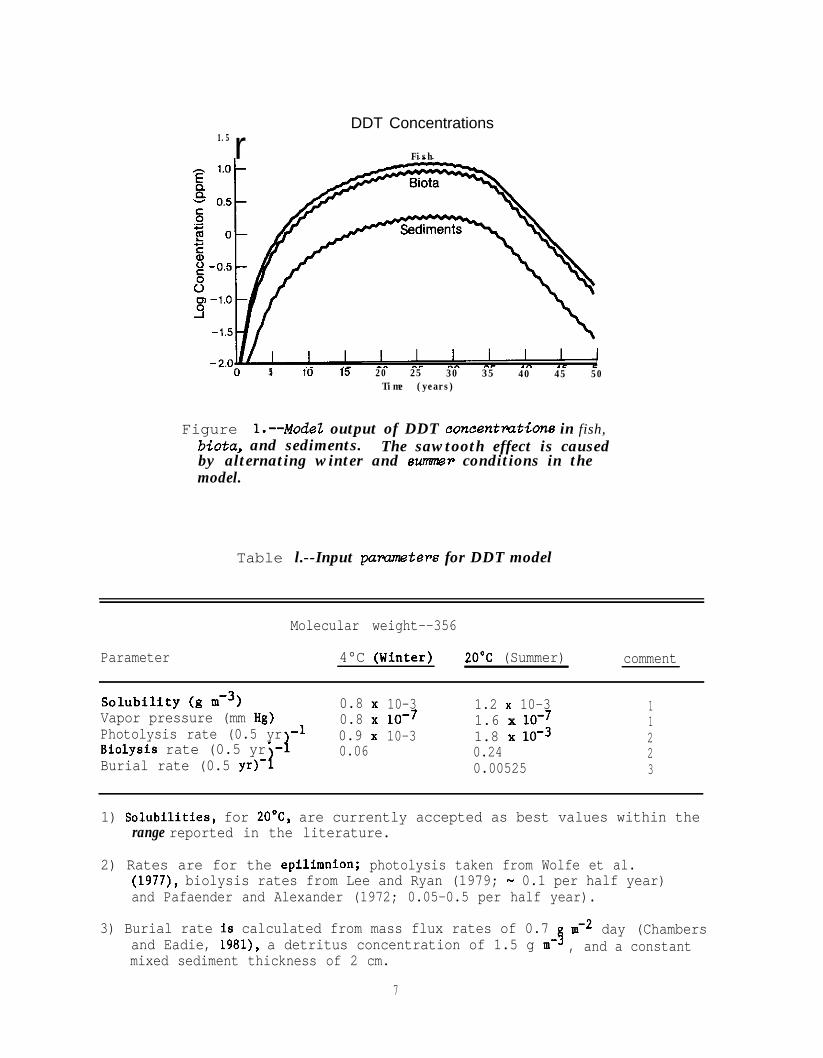
The model was run for DDT and a mixture of PCB's as Aroclors". Theresults are presented below. In the graphical output, winter conditionsimply that the epilimnion was kept at 4'C for all time steps and that micro-bial decomposition was one-quarter and photolysis one-half of the summercase. These winter/summer scenarios were designed to approximately span therange of decomposition rates in the literature. When the time steps werealternated between winter and summer conditions, the increase in solubilityand vapor pressure at the higher temperatures strongly affected the distri-bution as shown in figure 1.

The local maxima in the sediments and biota are the winter values. Themodel predicts an epilimnetic depletion of contaminant that can be testedwith a relatively modest field effort, currently being planned.

5.2 The Model Applied to DDT

DDT research is almost out of vogue; however, after the large amount ofmoney spent, some relatively basic information regarding the decompositionof the compound is on shaky ground. There is no clear information onloads; thus the model input was calibrated to concentrations reported inbloater chubs for Lake Michigan [International Joint Commission (IJC),19791. Information on solubility and vapor pressure as a function of tem-perature was not found; a difference of 50 percent was assumed between 4"and 20°C. This is less of a range than for many similar halogenated aro-matic hydrocarbons. The values used in the model are listed in table 1.

6

DDT Concentrations1.5 r Fish

I5 10 15 20 25 30 35 40 45 50

Time (years)

Figure I.--Model output of DDT concentmtione in fish,biota, and sediments. The sawtooth effect is causedby alternating winter and ewnmev conditions in themodel.

Table l.--Input pammeters for DDT model

Molecular weight--356

Parameter 4°C (Winter) 2o"c (Summer) comment

Solubility (g m-3) 0.8 x 10-3 1.2 x 10-3 1Vapor pressure (mm Hg) 0.8 x lO-7 1.6 x 1O-7 1Photolysis rate (0.5 yr ' 0.9 x 10-3 1.8 x lO-3 2Biolysis rate (0.5 yr 0.06 0.24 2Burial rate (0.5 yr)- 0.00525 3

1) Solubilities, for 2O"C, are currently accepted as best values within therange reported in the literature.

2) Rates are for the epilimnion; photolysis taken from Wolfe et al.(1977), biolysis rates from Lee and Ryan (1979; - 0.1 per half year)and Pafaender and Alexander (1972; 0.05-0.5 per half year).

3) Burial rate is calculated from mass flux rates of 0.7-3 mv2 day (Chambersand Eadie, 1981), a detritus concentration of 1.5 g m , and a constantmixed sediment thickness of 2 cm.

7

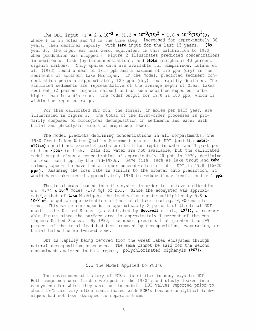
The DDT input (I - 2 x 10s3 x (1.2 x 10-3(TS)2 - 1.6 x 10-5(TS)3)),where I is in moles and TS is the time step, increased for approximately 30years, then declined rapidly, with zero input for the last 15 years. (BYyear 33, the input was near zero, equivalent in this calibration to 1970,when production was stopped.) Figure 2 illustrates predicted concentrationsin sediments, fish (by bioconcentration), and biota (sorption; 40 percentorganic carbon). Only sparse data are available for comparison. Leland etal. (1973) found a mean of 18.5 ppb and a maximum of 175 ppb (dry) in thesediments of southern Lake Michigan. In the model, predicted sediment con-centration peaks at approximately 120 ppb (dry), but rapidly declines. Thesimulated sediments are representative of the average depth of Great Lakessediment (2 percent organic carbon) and as such would be expected to behigher than Leland's mean. The model output for 1970 is 100 ppb, which iswithin the reported range.

For this calibrated DDT run, the losses, in moles per half year, areillustrated in figure 3. The total of the first-order processes is pri-marily composed of biological decomposition in sediments and water withburial and photolysis orders of magnitude lower.

The model predicts declining concentrations in all compartments. The1980 Great Lakes Water Quality Agreement states that DDT (and its metab-elites) should not exceed 3 parts per trillion (ppt) in water and 1 part permillion (ppm) in fish. Data for water are not available, but the calibratedmodel output gives a concentration of approximately 40 ppt in 1970, decliningto less than 1 ppt by the mid-1980s. Game fish, such as lake trout and cohosalmon, appear to have had a higher concentration of total DDT in 1970 (15-20PFQ). Assuming the loss rate is similar to the bloater chub prediction, itwould have taken until approximately 1980 to reduce those levels to the 1 ppm.

The total mass loaded into the system in order to achieve calibrationwas 4.74 x low4 moles (170 mg) of DDT. Since the ecosystem was approxi-mately that of Lake Michigan, the load value can be multiplied by 5.8 x101~ m2 to get an approximation of the total lake loading, 9,900 metrictons. This value corresponds to approximately 2 percent of the total DDTused in the United States (as estimated by Woodwell et al., 1971), a reason-able figure since the surface area is approximately 1 percent of the con-tiguous United States. By 1980, the model predicts that greater than 99percent of the total load had been removed by decomposition, evaporation, orburial below the well-mixed zone.

DDT is rapidly being removed from the Great Lakes ecosystem throughnatural decomposition processes. The same cannot be said for the secondcontaminant analyzed in this report, polychlorinated biphenyls (PCB).

5.3 The Model Applied to PCB's

The environmental history of PCB's is similar in many ways to DDT.Both compounds were first developed in the 1930's and slowly leaked intoecosystems for which they were not intended. DDT values reported prior toabout 1975 are very often contaminated with PCB's because analytical tech-niques had not been designed to separate them.

8

DDT Concentrations1.5r Fish

-z 1.0

g 0.5

s'=e 0.0

z2 -0.5

sv3 -1.0

-1.5

-2.0

1970 1980

Figure 2.--DDT concentrations. The lines are outputfrom a simulation using continuous summer condi-tione; points are data for bloater chubs and eedi-mente from Lake Michigan.

DDT Loss Rates

-12 I I I I I I I I I I0 5 ,O 15 20 25' 30 35 40 45 50

Time (years)

Figure 3.--DDT lose rates (mot8 per half year). ticro-bial decomposition is the rmjor loss.

9

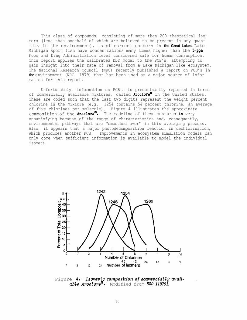
This class of compounds, consisting of more than 200 theoretical iso-mers (less than one-half of which are believed to be present in any quan-tity in the environment), is of current concern in the Great Lakes. LakeMichigan sport fish have concentrations many times higher than the 5-ppmFood and Drug Administration level considered safe for human consumption.This report applies the calibrated DDT model to the PCB’s, attempting togain insight into their rate of removal from a Lake Michigan-like ecosystem.The National Research Council (NRC) recently published a report on PCB’s inthe environment (NRC, 1979) that has been used as a major source of infor-mation for this report.

Unfortunately, information on PCB’s is predominantly reported in termsof commercially available mixtures, called AroclorsQ in the United States.These are coded such that the last two digits represent the weight percentchlorine in the mixture (e.g., 1254 contains 54 percent chlorine, an averageof five chlorines per molecule).composition of the Aroclorsm.

Figure 4 illustrates the approximateThe modeling of these mixtures is very

unsatisfying because of the range of characteristics and, consequently,environmental pathways that are “smoothed over” in this averaging process.Also, it appears that a major photodecomposition reaction is dechlorination,which produces another PCB. Improvements in ecosystem simulation models canonly come when sufficient information is available to model the individualisomers.

5 0 -

. 6 4 5 -

.%40-::E 35 -830-

zzs-

zzo-

-5El5-

a io-j 5:

O-0 2

I1 3 7 8 9 l o

1 3 12 24 4224 12 3 1

Number 2 Isonk

Figure 4.--Ieomeric composition of connnwaially avail-able Aroclors".

.Modified from NRC 119791.

10

The version of the model discussed in this report follows the movementof PCB mixtures 1242, 1248, 1254, and 1260. The model information is listedin table 2. The two temperatures and corresponding pairs of rate numbersand physical characteristics are designed to span a range that can beobtained from the literature. The low rates (winter conditions) are com-bined for the first run and the high rates (summer conditions) for thesecond run, producing an envelope of prediction.

Table 2.--Input parameter6 for PCB model

1242 1248 1254 1260 Comments

"Molecular weight" 258 290 324 375 1Temperature ("C) 1Solubility (g D-~)

4; 20 4; 20 4; 20 4; 200.20; 0.24 0.043; 0.054 0.010; 0.012 0.002; 0.003 2

Vapor pressure(mm Hg) x 104 1.5; 7.2 1.3; 6.3 0.28; 1.5 0.14; 0.75 3

Photolysis rate(0.5 yr)-l 0.05; 0.1 0.03; 0.06 0.02; 0.04 0.01; 0.02 4

Burial rate(0.5 yr)-l

Biolysis rate(0.5 yr)-l

0.005; 0.02 0.005; 0.02 0.005; 0.02 0.005; 0.02 5

0.5; 1. 0.2; 0.4 0.05; 0.1 0.01; 0.03

1) From NRC (1979).

2) Calculated from information in NRC (1979).

3) Estimated from Simmons (personal communication).

4) From Chambers and Eadie (1981); Robbins (personal communication).

5) Calculated from Rice (personal communication); Anderson (1980). Furukawaet al. (1978). See discussion on microbial decomposition rates fordissolved contaminant reduced by 10x (Lee and Ryan, 1979).

11

Individual process rates are often difficult to extrapolate from theliterature. Early results from GLERL's program at The University ofMichigan (Simmons, personal communication) provide the most realistic num-bers for photolysis. These have been subjectively combined with the resultsof Safe and Hutzinger (1971), Ruzo et al. (1972), Herring et al. (1972),Hutzinger et al. (1972), and Crosby and Moilanen (1973). Variations inexperimental conditions and exotic experimental procedures (from the pointof view of someone trying to extrapolate to an aquatic ecosystem) makeobjective comparisons impossible. Thus, the photolytic rate numbers intable 2 are comparatively weak at this time.

5.4 Microbial Degradation

The basic mechanisms involved in biodegradation of PCB's are differentfrom those found for DDT. The absence of an alkyl group between the benzenering in PCB's rules out the separation of the rings by cleaving the uncon-jugated bond. The typical mechanism described for PCB degradation consistsof hydroxylation, followed by ring fission, of the lesser-chlorinated ring.

One of the major drawbacks to direct application of laboratory rates tonatural systems is the type of organisms used in the rate-determinationexperiments. The first problem is the use of pure (or axenic) rather thanmixed cultures. Pure cultures do not exist in nature. The use of mixedcultures provides a better simulation of an environment where many types arepresent simultaneously, each representing unique intrinsic metabolic capa-bilities. The source of the cultures is also a weak point; most exponentsemploy enrichment isolation techniques that alter the population structureof the original culture.

Many researchers noted that degradation rates changed with time,increasing to a maximum as time progressed. This phenomenon, known as accli-mation, is not well understood in natural populations, but the occurrence ofhigher degradation rates for organisms from regions of chronic contaminationis fairly well documented. At the present time, acclimation (and ratechanges that are due to acclimation) in natural systems is an important partof the problem pertaining to the applicability of laboratory rates to ratesfound in the environment. From the limited evidence provided by a fewexperiments with simulated natural conditions, the difference in overallrates does not seem to be too substantial.

There are four identified major variables that have an effect ondegradation rates: (1) temperature, (2) type of organism, (3) cell con-centration, and (4) substrate (PCB) concentration.

Each type of bacterium will have an intrinsic rate of degradationspecific for that organism. (See Furukawa et al., 1978; Clark et al., 1979.)The bacteria that were tested in the experiments below had similar rates inmost cases. Another factor that would presumably be specific for each bac-terium is the induced rate, the rate following acclimation to the substrate.As stated above, acclimation times and their variablility are not known fornatural systems at the present time.

12

Furukawa and his co-workers showed that overall degradation ratesincrease with increasing cell concentration. They measured changes in therate of formation of a yellow compound, with a known absorption maximum,from a 4'substituted biphenyl (2,5,4'-trichlorobiphenyl) as the optical den-sity of the culture was increased. They found similar results with both ofthe cultures they tested: the amount of yellow compound formed increased toa maximum as the number of bacteria (optical density) increased. Boethlingand Alexander (1979) showed that degradation rates increased as substrateconcentration increased. While they used p-chlorobenzoate, chloroacetate,2,4-dichlorophenoxyacetate (2,4-D), and 1-naphthyl-N-methyl-carbamate (NMC),it is reasonable to believe that the results are generally applicable to PCBbiodegradation. They found that virtually no degradation occurred below athreshold concentration of 2 to 3 ng mL-l for ,2,4-D and NMC. At higher con-centrations, degradation (complete conversion to carbon dioxide) occurred ata rate of approximately 10 percent per day. For these experiments, micro-bial populations were collected from a stream in New York that drains agri-cultural runoff and receives treated sewage upstream from the sampling site.

Another important point raised by Boethling and Alexander (1979) wasthat extrapolation of rate information from high to low substrate con-centrations is not an accurate prediction of rates at low levels. Whenmeasuring complete degradation of 2,4-D to carbon dioxide, they found thatusing laboratory rates found for 22 mg mL-' and 220 ng mL -1 to predict therate at 2.2 ng mL-l (by assuming direct proportionality with substrateconcentration) yielded predicted rates that were more than one order ofmagnitude greater than actual laboratory rates.

Wong and Kaiser (1975) isolated bacteria from Hamilton Harbour, LakeOntario, and determined their ability to degrade PCB's. To isolate theseorganisms, they used media in which Aroclors" 1221, 1242, and 1254 were thesole carbon and energy source. All of their determinations were performedat 2o"c. With 0.05-percent solutions, no growth occurred on Aroclor" 1254,but degradation could be followed on 1221 and 1242. Wong and Kaiser foundthat the less-chlorinated compounds were degraded at a higher rate than themore highly chlorinated compounds. Thus, in experiments with single iso-mers, degradation rates could be arranged as follows: biphenyl >2-chlorobiphenyl > 4-chlorobiphenyl. They also observed that the positionof chlorination, as well as the degree of chlorination, was important indetermining the rate.

The bacterial population used in the Aroclor" 1221 experiment (summar-ized in table 3) started at approximately lo4 cells m~-l and reached anasymptotic maximum of LO7 cells rn~-l within 7 days, by which time up to 55percent of some of the gas chromatographic (GC) peaks had been degraded.This reduces to a rate of about 4 ng degraded cell-l day-', assuming that 55percent of the total PCB present was degraded by lo4 bacteria mL-' in 500 mLof solution in 7 days.

In another experiment, two species of bacteria were tested for theirability to degrade specific PCB isomers. Furukawa and his co-workers(Furukawa et al., 1978) used Alcaligenee sp. and Acinetobacter sp. isolatedfrom "aquatic sediment" by biphenyl and 4-cholorobiphenyl enrichment,

13

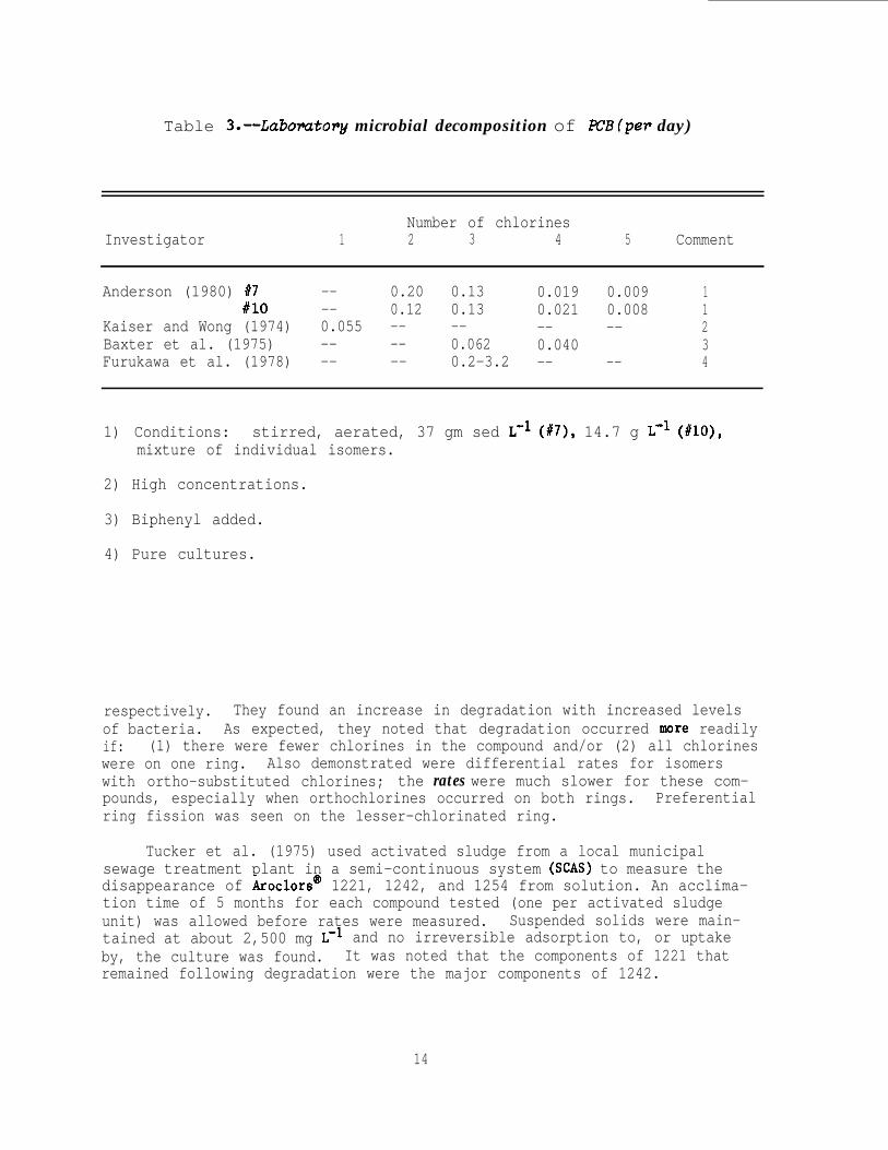
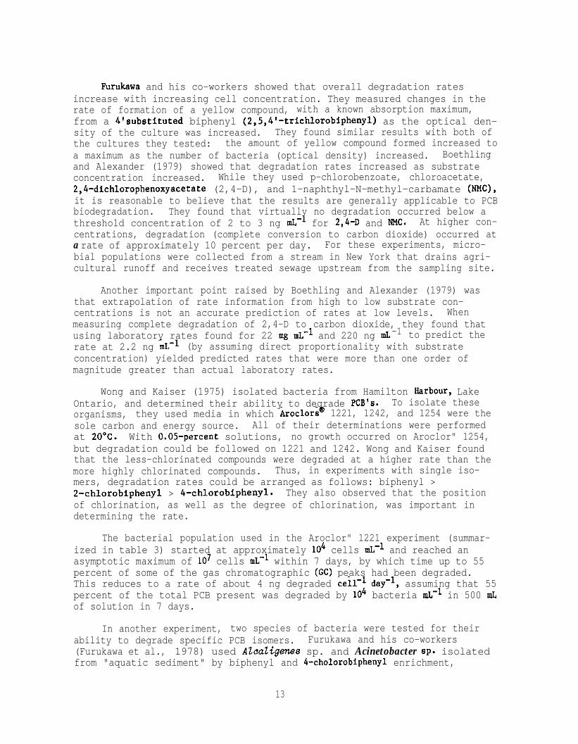
Table 3.--Labomtory microbial decomposition of EVE (per day)

Number of chlorinesInvestigator 1 2 3 4 5 Comment

Anderson (1980) #7 -- 0.20 0.13 0.019 0.009 1t10 -- 0.12 0.13 0.021 0.008 1

Kaiser and Wong (1974) 0.055 -- -- -- -- 2Baxter et al. (1975) -- -- 0.062 0.040 3Furukawa et al. (1978) -- -- 0.2-3.2 -- -- 4

1) Conditions: stirred, aerated, 37 gm sed L-l (#7), 14.7 g L-l (#lo).mixture of individual isomers.

2) High concentrations.

3) Biphenyl added.

4) Pure cultures.

respectively. They found an increase in degradation with increased levelsof bacteria. As expected, they noted that degradation occurred mOre readilyif: (1) there were fewer chlorines in the compound and/or (2) all chlorineswere on one ring. Also demonstrated were differential rates for isomerswith ortho-substituted chlorines; the rates were much slower for these com-pounds, especially when orthochlorines occurred on both rings. Preferentialring fission was seen on the lesser-chlorinated ring.

Tucker et al. (1975) used activated sludge from a local municipalsewage treatment plant in a semi-continuous system (SCAS) to measure thedisappearance of Aroclors@ 1221, 1242, and 1254 from solution. An acclima-tion time of 5 months for each compound tested (one per activated sludgeunit) was allowed before rates were measured.tained at about 2,500 mg L-l

Suspended solids were main-and no irreversible adsorption to, or uptake

by, the culture was found. It was noted that the components of 1221 thatremained following degradation were the major components of 1242.

14

Baxter et al. (1975) performed two series of experiments on each of twospecies of bacteria:10643, respectively*).

Nocadia sp. and Pseudomonas sp. (NCIB 10603 and NCIBThe first series consisted of simple systems con-

taining one, two, or three PCB isomers (some also included biphenyl), whilethe second was run with commercial mixtures along with excess biphenyl.Results showed that compounds with up to six chlorines could be degradedunder the proper conditions (in the presence of certain other isomers and/orbiphenyl, or as part of a commercial mixture). As before, the isomers withfewer chlorines were generally degraded faster.

Clark et al. (1979) experimented with a mixed culture of bacteriaobtained from polluted Hudson River sediment (the "Fort Miller disposalsite"). The most numerous organisms (in order of greater numbers) wereAlcaligenes odomns and AlCaligene8 denitrifioans. Again, lower chlorinatedisomers were degraded fastest, with differential rates according to theposition of chlorination.

Anderson (1980) reanalyzed the data from previous experiments andcalculated first-order rate constants. Ha also calculated first-order rateconstants from his own work using sediment suspensions from Saginaw Bay andmixtures of PCB's. The averaged results are summarized in table 3.

Intercomparison between investigators is difficult considering thevariations in experimental procedures employed. However, it is clear thatthe rates seem to agree fairly well, except for those of Furukawa et al.Their use of pure bacterial cultures known to degrade PCB isomers led topredictably high rates.

In summary, several main points can be extracted from all of theseexperiments:

(1) degradation decreases with increasing chlorination (ordecreasing water solubility);

(2) differential degradation occurs according to position ofchlorination;

(3) degradation increases with increased bacterial, and substrate,concentration; and

(4) degradation rates (for some compounds) change with certainisomeric combinations and with the addition of acetate orbiphenyl.

Several points must be kept in mind. First, all of the experimentsdescribed employed enrichment techniques of some sort, which obviouslychanged the populations. Second, most of the experiments were conducted atambient temperatures (20' to 25OC). Third, the PCB concentrations used in

*NCIB: National Collection of Industrial Bacteria

15

these experiments were much higher (on the order of hundreds of parts permillion) than those found in freshwater systems. Current PCB levels in theGreat Lakes are on the order of 10 ppt (water) to 100 ppb (sediments).

All of these indicate that natural rates should be lower than thosemeasured in laboratory experiments. Other arguments concerning theseresults also center around the cultures themselves. There is little doubtthat pure cultures do not exist in nature. The use of mixed natural popula-tions would be more appropriate to obtaining rates similar to those found innature. It is logical to assume that rates would be different in anenvironment in which a number of species participated in degradation.

A microbial decomposition rate can be estimated for Aroclor" mixturesfrom the isomer distribution illustrated in figure 4 and the biolysis ratesin table 3 as follows:

R1242 = 0.1 x R2 + 0.4 x R3 + 0.2 x R4 + 0.2 x R5 + 0.1 x R6,

where R2 = rate for dichlorobiphenyl (table 3). etc., and R6-9 = 0. Then

R1422 = 0.07 day-l = 12.6 (0.5 yr)-1

R1248 = 0.02 day-l = 3.6 (0.5 yr)-'

R1254 = 0.009 day-l = 1.6 (0.5 yr)-l

R1260 = 0.001 day-l = 0.25 (0.5 yr) ,-1

which yield reasonable laboratory rates. The deep water and sediment tem-peratures of the Great Lakes range from near zero to 4°C. This will leadto a reduction of at least an order of magnitude in the rate numbers (Leea& Ryan, 1979). The rates are probably high for other reasons cited above.

Considering the caveats, I have set the high rates equal to approxi-mately 10 percent of the laboratory values and the low rates at one-thirdthe value of the high rates.

6. RESULTS

Model output for sediments and biota are shown in figures 5 (winterconditions) and 6 (summer conditions). The winter condition is the resultof using the low rates in table 2 and is calibrated to yield a maximum con-centration of approximately 10 ppm in the biota. At the same time, sedimentconcentrations peak at approximately 75 ppb, a value within the rangereported for Lake Michigan (Konasewich et al., 1978). In order to obtainsimilar maximum concentrations, the summer condition run (figure 2) required20 times the load of PCB used for the winter case.

16

PCB in Biota; Winter Conditions

Total PCB

0

-1

E - 2,a

s‘x=49

-3

E

: -4n

’ “r (b)PCB in Sediments; Winter Conditions

Total PcB1

1260

1248

~‘~~~\-/I I I J0 5 10 15 20 25 30 35 40 45 50

Time (years)

Figure 5.--a) PCB mixtures in biota using the lowrates in table 2. The nwnbers refer to Aroclors' asdescribed in figure 6. The 1242 load is depictedto give a feeling for the shape of the input func-tion. The other Aroclore” have the came load fun+tion but a lower (0.25~) magnitude. b/ PCBmixtures in sediments for the same run.

17

r8s‘Gz5zs3

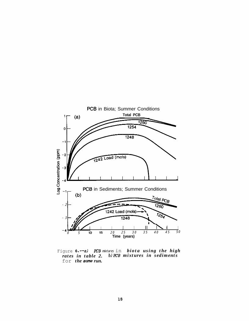
PC6 in Biota; Summer ConditionsTotal PCB

-17 PC6 in Sediments; Summer Conditions

- 2

- 3

‘,,, /

I (b)

I I I I II i\ I I0 5 10 15 2 0 2 5 3 0 3 5 4 0 4 5 5 0

Time (years)

Figure 6.--a) EB mixtures in biota using the highrates in table 2. bl PZ’B mixtures in sedimentsfor the cxzme run.

18

As for the DDT simulation, year 35 is approximately equal to 1972.Figure 7 compares model output for the winter and summer cases with PCB datafor Lake Michigan fish as summarized in Sonzogni et al. (1981). The modeloutputs can be moved up and down the page by altering the load, and the out-puts will remain very nearly parallel. The agreement with bloaters and cohosalmon is encouraging, considering the simplicity of the model. The laketrout data could not be simulated with a model as simple as this. Weininger(1978) proposed considerable food chain transfer from benthic organisms tolake trout and there is no food chain accumulation explicitly considered inthis model.

The model outputs indicate that the loss we are presently observing infish and sediments is primarily the lesser chlorinated isomers contained in1242 and 1248, whereas the Aroclors" 1254 and 1260 decay much more slowly.This scenario predicts an exponential approach to a lower concentration ofpredominately hexachlorinated and higher isomers that will remain for a longtime. The absolute value of this lower concentration strongly depends onthe present concentration of highly chlorinated isomers because atmospherictransport of such isomers is small and future loads are predicted to beSmall.

The loss rates from the ecosystem are illustrated in figure 8.Aroclors" 1242, 1254, and 1260 are shown; 1248 is intermediate between 1242and 1254, and was omitted for clarity. Atmospheric photolysis predominates,followed by microbial decomposition in the water and sediment. In theGreat Lakes, burial is a slow process, which is slowed by bioturbation. Themodel considered a general condition of a 2-cm-mixed thickness with 0.5- tol-mm accumulation per year. Assuming desorption occurs, the sediments canact as a source of stored hydrophobic contaminants for several decades.

19

24rLake Michigan Fish

Coho Salmon

0 I I I I I1972 1974 1976 1976 1960

Years

Figure 7.--Total PcB’e in Lake Michigan fish. Data aref r o m Konaeewich et al. (19781 and IJC 119791. Themodel outputs for biota from the runs illuetmted infigures la and 2a are shown as smooth curvea.

20

-4l-1242 Loss Rates; Summer Conditions

-1211254 LOSS Rates; Summer Conditions

-5

F

1260 LOSS Rates; Summer Conditions(c)

-6

0 5 10 16 20 25 30 35 40 45 50Time (years)

Figure a.--PCB toss mtes (mot per half year) from theammer scenario (figure 6). al Aroclo~@ 1242, blAroclor@ 1254, and cl Aroclor@ 1260 .

21

7. ACKNOWLEDGMENTS

Partial funding for this work "as provjded CIY the Office of MarimPollution Assessment (OMPA). We would like IX thank Dr. Bob Burns, directorof OMPA's Long Range Effects Research Program for his cooperation and Dr.Andrew Robertson for useful comments in re%lewlng this report.

22

a. REFERENCES

Anderson, M. L. (1980): Degradation of PCB in sediments of the GreatLakes. Ph.D. dissertation. Univ. of Mich., Ann Arbor. 256 pp.

Baxter, R. A., Gilbert, P. E., Lidgett, R. A., Mainprize, J. H., and Vodden,H. A. (1975): The degradation of polychlorinated biphenyls by micro-organisms. Sci. T o t a l Env. 4:53-61.

Boethling, R. S., and Alexander, M. (1979): Effect of concentration oforganic chemicals on their biodegradation by natural microbial con-munities. A p p t . a n d Env. M i c r o . 37(6):1211-1216.

Chambers, R. L., and Eadie, B. J. (1981): Nepheloid and suspended particulatematter in southeastern Lake Michigan. Sedimentotogy 28:439-447.

Clark, R. R., Chian, E. S. K., and Griffin, R. A. (1979): Degradation ofpolychlorinated biphenyls by nixed microbial cultures. Appt. and EnU.Micro. 37(4):680-685.

Crosby, D. G., and Moilanen, K. W. (1973): Photodecomposition ofchlorinated biphenyls and dibenzofurans. Bull. Env. Contam. a n dToxicol. 10(6):372-377.

Eadie, B. J. (1981): An equilibrium model for the partitioning of syntheticorganic compounds: Formulation and calibration, NOAA Tech. Memo.ERL GLERL-35. 44 pp.

Furukawa, K., Tononura, K.,'and Kamibayashi, A. (1978): Effect of chlorinesubstitution on the biodegradability of polychlorinated biphenyls.Appt. and Env. Micro. 35(2):223-227.

Herring, J. L., Hannan, E. J., and Bills, D. D. (1972): W irradiationof Aroclor" 1254. B u l l . Em. Contam. a n d ToxicoZ. 8(3):153-157.

Hutzinger, O., Safe, S., and Zitko, V. (1972): Photochemical degradation ofchlorobiphenyls (PCB's). Enu. Health Perepec. pp. 15-20 (April).

International Joint Commission. (1979): Great Lakes water quality:Seventh annual report to the International Joint Commission, GreatLakes Wat. Qual. Bd., Windsor, Oat.

Kaiser, K. L. E., and Wong, P. I. S. (1974): Bacterial degradation ofpolychlorinated bi henyls.ducts from Aroclor8

I. Identification of some metabolic pro-1242. Bull. Env. Contam. a n d Toxicol. 11(3):291-296.

Kooasewich, D., Traversy W., and Zar, H. (1978): Great Lakes waterquality: Status report on organic and heavy metal contaminants in LakesErie, Michigan, Huron, and Superior Basins, Great Lakes Wat. Qual. Bd.,Windsor, Ont.

23

Lee, R. F., and Ryan, C. (1979): Microbial degradation of organochlorinecompounds in estuarine waters and sediments. In: Proc. of theworkshop: Microbial Degradation of Pollutants in Marine Enoironmente,EPA report % EPA-600/9-79-012, National Technical Information Service,Springfield, Va. 22151.

Leland, H. V., Bruce, W. N., and Shimp, N. F. (1973): Chlorinated hydrocar-bon insecticides in sediments of southern Lake Michigan. Em. Sci. and~~42. 7:833-838.

Mackay, D. (1979): Finding fugacity feasible. Enu. Soi. and Tech.13:1218-1223.

National Research Council. (1979): Polychlorinated biphenyls. Nat. Acad.of sci., Washington, D.C., 182 pp.

Pfaender, F. K., and Alexander, M. (1972): Extensive microbial degradationof DDT in vitro and DDT metabolism by natural communities. J. Agr.Food Chem. 20:842-846.

Peakall, D. B., and Lincer, J. L. (1970): Polychlorinated biphenyls:Another long-life widespread chemical in the environment. B&Science20(17):958-964.

Ruzo, L. O., Zabik, M. J., and Schuetz, R. D. (1972): Polychlorinatedbiphenyls: Photolysis of 3,4,3',4'-tetrachlorobiphenyl and4,4'-dichlorobiphenyl in solution. Bull . of Em. Contam. and Toxicol .8(4):217-218.

Safe, S., and +tzinger, 0. (1971): Polychlorinated biphenyls: Photolysisof 2,4,6,2',4',6'-hexachlorobiphenyl. Nature 232:641-642.

Sonzogni, W. C., Simmons, M., Smith, S., and Rice, C. (1981): A criticalreview of available data on organic and heavy metal contaminants in theGreat Lakes, Great Lakes Basin Comm., Ann Arbor.

Tucker, E. S., Saeger, V. W., and Hicks, 0. (1975): Activated sludge pri-mary biodegradation of polychlorinated biphenyls. Bull. Env. Contam.and Toxicol. 14(6):705-713.

Weininger, D. (1978): Accumulation of PCB's by lake trout in Lake Michigan.Ph.D. dissertation. Univ. of Wis., Madison. 232 pp.

Wolfe, N. L., Zepp, R. G., Paris, D. F., Baughman, G. L., and Hollis, R. C.(1977): Methoxychlor and DDT degradation in water: Rates andProducts. Em. Sci. und Tech. 11:1077-1081.

Wong, P. T. S., and Kaiser, K. L. E. (1975): Bacterial degradation of poly-chlorinated biphenyls. II. Rate Studies. Butt. Gnu. Contam. andToxicol. 13(2):249-256.

Woodwell, G. M., Craig, P. P., and Johnson, H. A. (1971): DDT in thebiosphere: Where does it go? Science 174:1101-1107.

24

9. Appendix--PROGRAM OUTPUT

tiET.FUGKOD3/COPY,FUGllOD3

PROGRAM tiOD2 lINPUT.OUTPUT~TAPE3,TAPE5=INPUT,TAPEblC tiINENSION OF A y B. Al, A2 II R ARRAYS MUST BE (NT,W OF VARIABLES1c THESE ARRAYS ARE FOR PLOTTING ROUTINES

DIKENSION A1(100,101,62(100,101,TE1011001,TSED~1001DIKENSION R~100;i01,N0120I,A~100,91,d(100,81COtlllON /INDAAT/ S~5121,TK~2~,~U~5~,AA0,BB0COHKON /INFO/ LC,Z~8).VP~5).Hl5l,OC~8l~V~81COKKON /RATE/ PK(5.811BK(5~8)COKKON /INDEX/ I,J,K.JJ,NC,NT,NXCOtlKON /PARK/ TN~101,51,CN~8,100,51,PK18,100,51,CC~8,100~51COKKON /LOSS/ TLOSS~Jl,SD~100,5l,TL~lOO,~,~BD~8,lOO,5l,PD~8,lOO,5lCOKKON /INTO/ XI5),TINPUTl100,5),TLOADllOO,5l

CDATA A /900 1 -999./DATA B /800 * -999.1'DATA R /lOOO * -999./DATA Al /lOOO * -999.1DATA A2 /lo00 : -999.1

C THE ABOVE PRESET THE PLOTTIN ARRAYS ; DINENSIONS KUST BE EXACTCC **** ALL INPUT DATA IS IN THIS SECTION ***

* CALIBRATION DATA FOR DDT *DATA TK /275.,293./

TK = TEKPERATURES FOR THE TYO TINE STEPSDATA S /S*O.BE-3,5:1.2E-31

S = SOLUBILITY(G/N31 ; 5 CONTAWINENTS ; 2 TLllPSDATA NU /5*35bf

KU = KOLECULAR UEIONTSDATA PK /3.bE-3,7.2E-3,1.8E-3,2*3.bE-3,l.BE-3,3.bE-3,0.9E-3,12*1.8E-3,30*0./

PHOTOLYSIS RATE CONSTANTS (PER .5 YRlDATA BK /5*0.,7*I~.24,0.24,0.24,0.48,0.121/

BIOLOGIGAL LOSS RATES (KOL/K3/0.5YRlDATA X /5*2E-3/

x SCALES T HE LOAD FUNCTION ; x * SINlTINE**ZlVAPOR PRESSURE cnn HG)

DATA UP /5*1.bE-71

; SET UP UITH TECKTRONIX TERKINAL GRAPHICS OUTPUTCC EGUILIBRIUK llODEL(FUGACITY1 DESIGNED TO TAKE O.SYEAR Tlr(E STEPSCC

2 5

CCcCC

CCCCC

CCCC

CC

C

C

C

C

C

C

C

C

C

CC

C

MODEL UNITS ARE IN nOLS ; EXCEPT CCtI,J,K) UNICH IS G/n3S = SOLUBILITIES OF AROCLORS 1242-1260 AT 2 L 20 DEG C (0043)

INTERACTlUE INhJT

IJK

PRINT*,"ENTER THE NUHBER OF TIHE STEPS (100 MAX)"REIID*,NTPRINT*,"ENTER THE l!UnRER OF COMPOUNDS (5 AAX)"READ*,NX

IS THE COnPARTnENT INDEXIS THE TInE STEPIS THE CONPOUND INDEX

R = S2E-6TL = TOThL LOSS OF CONTAnINENT ; Ttl = TOTAL MASS

DESCRIBE THE ECOSYSTEn

NC = 7NC = NUMBER OF COW6RTnENTS1 = dTnOSPHERE (10 Kn X ln2)

U(t) = 1E42 = EPILInNION (25113

U(2) = 253 = HYPOLInNION (7511)

U(3) = 754 = DETRITUS (l.SPP~;10XOR6.c)

U(4) = l.SE-4S = BIOTA (SO nG/ti2)

U(5) = SE-66 = SEDIMENTS (2cn nIXED,2% DRG C)

U(6) = 2E-27 = FISH ; USING I\ BIOCONCENTRATION FACTOR

'J(7) = ZE-7PERCENT ORGhNIC CARBON INPUT

OC(4) = 10OC(S) = 40OC(6) = 2

DO 5 K = 1,NXTLOSStK) = 0.

5 TLOAD(l,K) = 0.DO 100 J = 1,NTDO 100 K * 1,NX

CALL LOAD

JJ = 1 FOR UNSTRITIFIED(YINTER; = 2 FOR SUWKERJJ = 2 - (J-(J/21*2)JJ = 2

CALCULlTE HENRYS CONSTllNTH(K) = (UP(K)/760)/(S(K,JJ)/nU(K))

26

C

C

C

CC

C

C

CC

C

CCCC

CC

CC

CC

CALCULATE 2 VALUES FOR EACH COWPARTtiENTZ(l) = l/LR*TK(JJ))Z(2) = l/H(K)Z(3) = l/((VPLK)/760) / (S4K,lT/tlULK))T

HYPOLIGNION(3) IS HELD AT 2 DEG CDO 20 I = 4,b

20 Z(I) * 1O:~~4.75-0.70~AL0GlO~S~K,JJ~r1000/nU~K~~~*.Ol*OC~Il/H~K~BIOCONCENTRATION FACTOR CALCULATION

Z(7) = 6r10tr~3.5-0.54*AL0810(6(K,JJ)a1000/nU(KTTT/H~KTZ(6) = 0.05 * Z(6)

PARTITION COEFFICIENT IN SEDIMENTS LOUER BY FACTOR OF 20CALCULATE THE FUGACITY

SUKF ~0.DO 30 I * 1,NC

30 SUNF = sunF t v(z) I z(I)F = TliLJ,KT/SUKF

CALCULATE THE EQUILIBRIUW DISTRIBUTIONDO 40 I = 1,NCCH(I.J,K) = F*U(I)*Z(Il

CALCULATE COKPARTKENT CONCENTRATIONS40 CC(I,J,K) = CK(I,J,KT*KU(K)/V(I)

CALL DECAY

100 CONTINUE

CALL OUTPUT

FILLING ARRAYS FDn PLOT

DO 300 K = 1,NX

FILLING A ARRAY ; COKPARTHEMT CONCENTRATIONSDO 250 J = 1,NTA(J,l) = J1FtTINPUTtJ.K) .GT. 0.) A(J,2) 8 ALOGlO(TINPUT(J,KTTDO 250 I = 1, NC

250 IF(CC(I,J,K) .GT. 0.) A(J,I*2) = ALDGlO(CC(I,J,K)T

FILLING R ARRAY ; CONTAKINENT LOSSEStHOLSTDO 280 J = l,NTR(J,l) = JIF(SD(J,K) .GT. 0.) R(J,2) = ALOGlOlSD(J,K)TDO 260 I = 1,2

2 6 0 IF(PD(IIJ,K) .GT. 0.1 R(J,1+2) = ALOG101PD(I,J,K))DO 270 I = 2,b

270 IF(BD(I,J,K) .GT. 0.) R(J,I+S) = ALOGtO(BD(I,J,K)T280 IF(TL(J,K) .GT. 0.1 R(J,lO) = ALDGlO(TL(J,KT)

L

300 CONTINUEC FILLING B ARRAYC

27

C FILLING Al ARRAY ;C

DO 400 J = 1,NTTEIO(J1 i 0.Al(J,l) = JDO 401 K = 1,NX

IOTAL CONC IN BIOTA

401 IF(TINPUT(J,Kl .GT. 0.1 Al(J,K+l) = ALOGlOIf!U(K) * TINPUT(J,KllDO 400 K = l.NXTBIOtJ) = TBiOtJ) t CCIS,J,K)IF(CC(J,J,Kl .6T. 0.) Al(J,KtS) = ALOGlO(CCtS,J,K))

400 IF(TUIO(Jl .GT. 0.) Al(J,lO) = ALOGlO~TBID~J))CC FILLING A2 ARh,+Y ; SEDINENT CONCENTRATIONS

DO 500 J = 1,NTTSEDfJ) = 0.A2(J,i) = JDO 501 K = 1,NX

501 IF(TINPUT(J,K) .GT. 0.) A2(J,Ktll = ALOGlO( KU(K) *TINPUT(J,K))DO 500 K = 1,NXT&D(J) = TSEBfJ) * CC(b,J,K)IFlCC(6,J.K) .GT. 0.) A2(J,K+5) = ALOGlO(CC(b,J,K))

500 IF(TSED(J) .GT. 0.) A2(J,lO) = ALDOlO(TSED(J11CCC URITE ARRAY(J,VARIABLE) FOR TECKTRONIX PLOTC OUTPUT URITTEN ON FILE TAPEb=NOUC TO SUBMIT , REPLACE,TAPEb=NOU , THEN CALL,SUB(F=TEKPLT)C

REUIND 6DO 600 J = 1,NTDO 599 I = I,10

599 IF(A(J,I) .LT. -2.) A(J,Il = -2.C600 URITEl6)~A~J.l),A~J,2),A~J,4),b(J,S),A~J,b~,A~J~S~,A~J,91~

CSTOPEN3

28

SUBROUTINE DECAYLrlnHON /RATE/ PK(S,E),BK(S,B)COnnON /BAL/ THERE(lOO,S)COnnON IINDAAT/ S~5,2~,TK~2l,KU~5~,AA~S~,))(5~COnnDN /LOSS/ TLOSS~Sl,SD~100,5~,TL~lOO,S~,BD~B,lOO,S~,PD~B,lOO,S~COMON /PARN/ TH~101,S~,CK~G,100,5~,PH~G,lOO,5~,CC~G,lOO,~~COnHON /INDEX/ I,J,K,JJ,NC,NT,NXCOIIHON /INFO/ LC,Z(B),UP(S),N(5),0C(G),U(B)

CC PK 6 BK ARE PHOTOLYTIC D BIOLOOICAL DECOHPOSITION RAfES(CHPD,CNPTlCC UNITS PK(O.JYR-0 , BK(nOL/H3/0.SYR)C ASSUMPTIONS IN BIO CALC ; KICROBIAL DENSITY = ZOCELLWKL 1 lE6/KLC IN IJATER 6 SEDInENTS RESPECTIVELYCC CALCULATE PHOTOLYTIC DECAY

DO 20 I = I,NCC PR REDUCES UINTER RATES BY l/2

PR = 1.0IF(JJ.EO.l)PR=O.JPD(I.JfK) = CK(I,J,K) : (PR l PK(K,I))

20 IF(PD(I,J,K).OT.CH(I,J,K)) PD(I,J,K) = CH(I,J,K)c NECESSARY FOR nnss BALANCECC CALCULATE BIOLOGICAL DECAY

DO 10 I = 1,NCCLOUT = 1.0IF(JJ.EO.1) CLOUT = 0.25

C THAT REDUCES UINTER RATES BY A FACTOR OF 4VIABLE = 1

C FRACTION OF VIABLE BACTERIABD(,,J,K) = VIABLE * CLOUT * BK(K,I) 1 CH(I,J,K)

10 IF(BD(I,J,K).OT. (Cn(I,J,K) - PD(I,J,K))) BD(I,J,K) = CH(I,J,K)1- PD(I,J,K)

C NECESSARY FOR HASS BALANCECCC CALCULATE THE NEU CONCENTRATION

DO 30 I = 1,NCCn(1.J.K) = CH(I,J,K) - (BD(I,J,K) + PD(I,J,K))IF(CH(I,J,K) .LE. 0.) CH(I,J,K) = 0.

30 CC(I,J,K) = CK(I,J,K) t W(K) / 'J(I)CC CALCULATE SEDIHENT ALTERATION ; RECEIVES 50% OF DETRITUS PER TIHEC STEP ; THICKNESS REHAINS CONSTANT

SD(J,K) = 0.375 * Cn(6,J,K) / 1~0.CHL6,J,K) = 99.625*CH(b,J,K)/lOO. + O.S*CH(4,J,K)CH(4,J,K) = 0.5 t CH(4,J,K)

C SD = HASS (noL) BURIED IN DEEP SEDIHENTSCC(6,J,K) = Cn(6,J,K) * nU(K) / U(6)

C

29

C CALCULATE NEU TOTAL MASS '.TH(J,K) = 0.TL(J,K) = 0.DO 40 I = 1,NCTll(J,K) s Tll(J,K) + CIiLI,J,Kl

40 TL(J,KT = TL(J,Kl t BDLI,J,KT t PD(I,J,KITLLJ,KT = TL(J,KI + SDLJ,Kl

C TL = MASS OF REMOVED CONTAIIINENTC THERE = HASS IN SYBTEK + SYSTEM LOSSESC

DO 44 I * 1,NC44 PllII,J,K) * 100. * CtlLI,J,Kl/TMJ,KT

C P!l IS THE PERCENTAGE DISTRIBUTIONCC SUKKING UP LDSSES

TLOSSCK) = TLOSSCK) + TL(J,K)THERE(J,K) = TK(J,Kl + TLOSSLKlRETURNEND

EOI ENCOUNTERED.

/GET,LOADZ/COPY,LOADZ

SUBROUTINE LOADCOGKON /INTO/ X~51,TINPUT(t00,5I,TLOAD(100,5)COMON /INDEX/ I,J,K,JJ,NC,NT,NXCOMON /PARK/ TH~101,5~,CH~8,100,5~,P~~8,100,5~,CC~8,100,5~CDKGON /INDAAT/ S~5,2l,TK~2l,KU~S),AA~S),BB~S)

CC ROUTINE INCREASES TOTAL CONPDUND MA88 EACH TIME STEP

iINPUTIJ,Kl = (X(K) / Ml(K) * (l.PE-3*J*J - l.bE-S*J*J*J)lIF(TINPUT(J,Kl .LE. O.TTINPUT(J,KT = 0.IF(J.EQ.1)6,7

b TK(l,K) = TINPUT(l,KlGO TO 8

7 TH(J,Kl = TN(J-1,KI t TINPUTLJ,Kl8 CONTINUE

CIFLJ.EQ.11 TLOADLJ,Kl = TINPUT(l,K) + TMl,KlIFLJ.GT.11 TLDAD(J,K) = TLOADLJ-1,K) t TINPUTLJ,KT

CRETURNEND

EOI ENCOUNTERED.

3 0

/GET,OUTPUTP/COPY,OUTPUTZ

SUBROUTINE OUTPUTCONKON /LOSS/ TL~SS~5~,SD~100,5~,TL~lOO,S~,BD~8,lOO,5l,PD~8,lOO,S~COKGON /BAL/ THERE(lOO,STCOGKON /PART!/ T~~101,5~,CK~G,100,5~,PN~8,100,5~,CC~S,100,5~COtlKON /INDEX/ I,J,K,JJ,NC,NT,NXCOKKON /INTO/ X~S~,TINPUT~lOO,ST,TLOAD~lOO,S~COHKON /INFO/ LC,Z(8),VP(S),H(J),OC(8),V(8)

CC CONTROLS PROGRAM OUTPUT FOR FUGHODC

1

7

2

JSKIP = (NT - 2)/2DO 100 J = l,NT,JSKIPPRINT l,JFORflAT~///,"TIKE STEP =",14,/)DO 100 K = 1,NXPRINT 7FORtlAT(/,2OX,"SYSTEW NASS BALANCE (NOLST")PRINT 2,TINPUTCJ,K),TK(J,K),TL(J,H)FORKAT(/,"T STEP LOAD =",EB.3,' TOTAL IIASS IN SYSTEG =",E8.3,

1 " STEP LOSS =",EG.3)PRINT lS,TLOAD(J,K),THERE(J,KT

15 FORKAT("T0 DATE:INPUT=*,E12.4,4X,"AHT TRACED=",El2.4,/)PRINT 8

8 FORKAT("INDICES CONTANINENT DISTRIBUTION",bX,"LOSS RATES(NOL/"I"0 SYR)")PR;NT 3

3 FORKAT(" I KU,4X,"CK~HOL~",3X,"PW(Z~",SX,~CC~PPn)"l3X,~BIO~,7X,1"PHOTO",5X,"SED",BX,"Z",/)DO 91 1 9 1,NCSED = 0.IF(I.EQ.NC) SED = SD(J,KTPRINT 4,I,K,CK(I,J,K),PN(I,J,K),CC(I,J,K),BD(I,J,K),PD~I,J,K)

l,SED,Z(IT4 FORGAT(213,7El0.2T

91 CONTINUE100 CONTINUE

RETURNEND

ED1 ENCOUNTERED.

31

/GET,TEKPLT/COPY,TEKPLT/JOB/NOSE0PCBPLOT,TlfO.ACCOUNT,GL14,VERDA,GERL.CHARGE,RJ,1766212.FTN,R=2.GET,TAPES=NOU.CALL,BEPLOT.REPLACE,TAPEZ=PLQT.GDTO,l.EXIT.l,GET,SAVRSLT/UN=SLERL.DAYFILE,DAY.REPLACE,DAY.CALL.SAVRSLT(RESULT~BJESAV)

BJE.

JEORPROGRAM PCB(INPUT,OUTPUT,TAPES~TAPE2)DIKENSION A~100,10),TL100)

C READ DATA 1ST VARIABLE IS INDEPENDEKiREUIND 5

CC NPLT = NUMBER OF PLOTSCC NP = NUKBER OF DEPENDENT VARIABLES ON SINOLE GRAPH

NP = 7

DO 1 J = 1,1001 READ(S) (ALJ,I),I=l,NP)

f I LOOP IS THE NUNBER OF PARNS BEING PLOTTEDC RESTRUCTURING ARRAYS

T(1) = 0.DO 10 J = I,99

10 TLJtl) = FLOAT(J) / 2.C

32

C TECKTRDNIX PLOTTING GARBAGECALL IDC" BJES',TOOTCALL TEKTRN~"AUTOHC=YES,GAUD=24OO,CENTER,BATCH,TERM=4014,END~~,

1100)CALL BGNPLLl)CALL NOCHEKCALL TITLELIH ,-1,"T1KE(YEAR9)R*,100,"L06 CONCENTRATIONLPPK)S*,1100.10..7.)CALL GRAF(O.,S.,SO.,-2.,.5,2.1CALL KESSAG('DDT CONCENTRATIONS;UINTER CONDITION8",3B,2.,6.S)

CDO 20 I = l,NPIF(I.EQ.2) CALL DOTIF(I.EQ.3) CALL CHNDOTIF(I.EQ.4) CALL DASH1FLI.EQ.S) CALL CHNDSN1FLI.EQ.b) CALL RESET("CNNDSH")

20 CALL CURUE~T,A~1,1),100,0)CALL ENDPLC-1)CALL DONEPLSTOPEND

EOI ENCOUNTERED.

33

/GET,SUBSZfCOPY,SL!BS2BREADP LOAD2 DECAY2 OUTPUT2EEOI ENCOUNTERED.

/

/GET,RUN3/COPY,RUN3GET,FUGHOD3.GET,SUBSZ.XEDIT,FUGtlOD3,I=SUBS2.nEUIND,LGO.FTN,I=FUGHOD3,L=O,PND.GET,FUGtlOD3.LGO.OP=T.COPY,OUTPUTED1 ENCOUNTERED.

34