noao newsleter (december 2008) 13 kpno reu 09 annual .pdf · isochrones. white dwarf candidates...

NOAO NEWSLETER (DECEMBER 2008)

Annual Report 2008 REU Site Program at KPNO48

PUBLICATIONS AND PRODUCTS


Monday, January 5, 2009

A Wavelet Time Series Analysis of Aperiodic Variable Stars in the Kepler Field

Timothy Arnold (The Ohio State University) , K. Mighell (NOAO), S. Howell (NOAO)

The variable sky offers insights into the physical mechanisms of astronomical objects and can be

used as a useful tool for many other purposes like the determination of distance with standard

candles. Periodic variables were the first to be classified, understood, and used. Many variable but aperiodic light curves are discarded or insufficiently analyzed because of the apparent uselessness

of the information contained in these data. Many contemporary projects (e.g. the Large Synoptic

Survey Telescope, PanSTARRS, the Kepler mission) aim to map the transient sky, and recently

methods of time series analysis have become increasingly advanced. It would be advantageous to discover identifying information in the large number of variable but ostensibly aperiodic light

curves. We use a wavelet analysis, based on a weighted projection of time series data on to basis

functions, to analyze aperiodic variable stars in the Burrell-Optical-Kepler Survey (BOKS). Using the Weighted Wavelet Z-Transform detailed in Foster 1996, we find that variable but aperiodic stars

in our sample offer few characteristic properties that would be useful for further classification.

Arnold's research was supported by the NOAO/KPNO Research Experiences for Undergraduates (REU) Program which is funded by the National Science Foundation Research Experiences for

Undergraduates Program and the Department of Defense ASSURE program through Scientific

Program Order No. 3 (AST-0754223) of the Cooperative Agreement No. AST-0132798

between the Association of Universities for Research in Astronomy (AURA) and the NSF.



Research in Astronomy (AURA) and the NSF.

Wednesday, January 7, 2009

[474.03] Analyzing the Effects of Scattered Light on Stellar Photometry

Ashley Stewart (University of Arkansas, Fayetteville), J. Glaspey (NOAO)

The CCD detectors that we use today are very good at converting most of the light gathered by a

telescope into an electronic signal without adding much noise to the process. What this means for

observers is that they are now only limited by the optical quality of the telescope in how well they can measure the brightness of faint sources. Our goal was to quantify the affect of the scattered light

component of telescope images, usually dominated by the quality of primary mirror coating, using

empirically derived models of stellar Point Spread Functions for ground based imagers. We

analyzed archived MOSAIC data from the W-Project, which used the Blanco 4m telescope in Cerro Tololo, primarily because it covered the same fields over multiple years using the same telescope,

instruments, filters, and exposure times. From this data set, we selected stars using Source Extractor

and performed the photometry with the IRAF package DAOPHOT. This gave an estimate of the magnitudes and magnitude errors of the stars in the fields which could be compared for data taken

before and after primary mirror re-aluminizing. Here, we will present the findings of our project and

discuss what future work could be done to improve the quality of science obtained from ground

based telescopes.Stewart's research was supported by the NOAO/KPNO Research Experiences for Undergraduates (REU) Program, which is funded by the National Science Foundation Research

Experiences for Undergraduates Program and the Department of Defense ASSURE program

through Scientific Program Order No. 3 (AST-0754223) of the Cooperative Agreement No. AST-0132798 between the Association of Universities for Research in Astronomy (AURA) and the NSF.

Tuesday, January 6, 2009

[443.02] Investigating Galaxy Merger Signatures with IGNITE

Matthew J. Zagursky (University of Maryland), J. M. Lotz (NOAO)

I present the software package IGNITE, the Interacting Galaxy Non-Interactive Tail Extractor. Its

purpose is to locate tidal tails and quantify their morphological and photometric properties. I

demonstrate the effective use of IGNITE on the case galaxy of NGC 2623 and report the photometric and morphological signatures of tidal tails in this galaxy. The future of the IGNITE

package is a merge with other successful software packages aimed at quantifying merging galaxies

to further enhance the accuracy of the quantitative measurements of morphologies and photometry

profiles of merging galaxy candidates.



Monday, January 5, 2009

[414.03] Collinder 121: Analyzing It's Pre-main Sequence Population

Matthew Henderson (NOAO), W. Sherry (NSO)

OB associations represent excellent opportunities to study the end products of stellar accretion. These diffuse groups of stars, whose lifespans are limited by the dispersive forces that scatter them

as they move through the galaxy, are thought to be the structures in which the majority of all stars

form. We present a VI photometric census of the regions surrounding some of the stars identified by de Zeeuw et al. (1999) to be part of Collinder 121 (CMa OB2). Orion OB1 includes a clustered

population of low-mass, pre-main sequence stars present in the regions around the OB stars that

define the group. This study demonstrates whether a clustered population of low-mass, PMS stars exists in CMa OB2 and determines if the spatial pattern observed in Orion can be extended to

another OB association in the solar neighborhood.Matt Henderson’s research was supported by the

NOAO/KPNO Research Experiences for Undergraduates (REU) Program which is funded by the

National Science Foundation Research Experiences for Undergraduates Program and the Department of Defense ASSURE program through Scientific Program Order No. 3 (AST-0754223)

of the Cooperative Agreement No. AST-0132798 between the Association of Universities for

Research in Astronomy (AURA) and the NSF.


[442.12] Deep Photometry of the Open Cluster IC4651

Tiffany Meshkat (NOAO), C. Claver (NOAO), K. Mighell (NOAO)

We present a preliminary analysis of deep CCD photometry of the Galactic open star cluster IC

4651. We seek to identify the white dwarf cluster members in order to determine the age, distance, metallicity of the star cluster and to test stellar evolutionary theory. Claver observed IC 4651 at the

CTIO 4-meter telescope in Chile on May 7 - 10, 1997. The star cluster was covered by four camera

fields with small overlapping regions; one field was observed each night. Long and short exposures were obtained with U, B, V, and I filters in each field. Two of the nights were photometric with

subarsecond seeing, and the remaining two nights were not photometric. Stellar photometry was

obtained using the DAOPHOT procedure within IRAF data reduction and analysis system.

Calibrated photometry in all 4 fields was obtained using IRAF’s PHOTCAL package with the DAOPHOT instrumental magnitudes and standard star fit files. We made calibrated color-

magnitude diagrams and color-color diagrams in all four fields. The distance modulus was

determined to be (m-M) = 10.015 magnitudes, making IC4651 approximately 1000 pc away. The V vs. V-I color-magnitude diagram of IC 4651 is bracketed by the 1.5 Gyr and 2.0 Gyr Yonsei-Yi

isochrones. White dwarf candidates were determined by selecting stars near the cooling sequences

for DA 0.5 and 0.9 solar-mass white dwarfs; several of these white dwarf candidates fit the cooling

sequences within one standard deviation errorbars. Meshkat’s research was supported by the NOAO/KPNO Research Experiences for Undergraduates (REU) Program which is funded by the

National Science Foundation Research Experiences for Undergraduates Program and the

Department of Defense ASSURE program through Scientific Program Order No. 3 (AST-0754223)of the Cooperative Agreement No. AST-0132798 between the Association of Universities for



KPNO REU Students at the 213rd

AAS Meeting

January 2009

The opportunity to present the findings of their original research at the most important national

meeting of US astronomy is arguably one of the most prized benefits enjoyed by KPNO REU students. All six of the 2008 summer students will attend the 213rd meeting of the American

Astronomical Society (AAS) at Long Beach, California in January 2009. The students attending the

AAS meeting at Long Beach will also present posters incorporating aspects of their REU summer

research projects. Abstracts of the REU papers for the January AAS meeting are accessible at theAAS web site for the meeting; all will be published in the Bulletin of the American Astronomical

Society, Vol. 41, No. 1, 2009. The abstracts of the REU student posters are reproduced below.


[460.24] Site Characterization of El Peñón: The Site of the Large Synoptic Survey Telescope

Taylor S. Chonis (University of Nebraska-Lincoln Dept. of Physics and Astronomy) , C. F. Claver

(NOAO), J. Sebag (NOAO)

El Peñón is located at the southwest end of the Cerro Pachón ridge in northern Chile. Since its

selection as the LSST observatory site, detailed measurements of wind and atmospheric seeing have been conducted to help determine design and operating parameters. The wind measurements are

made at 4 elevations (5, 12, 20, 30 meters) using ultrasonic 3-axis anemometers. The atmospheric

seeing is monitored with a Differential Image Motion Monitor (DIMM). We have studied

correlations in the wind speed and direction at the different elevations and with the atmospheric seeing. From the wind-elevation correlations, we find evidence for a surface turbulence layer up to

a minimum of 12 meters above the local topography. Knowing where the boundary layer is will

affect the overall height of telescope and the summit building. In examining the correlation of image quality from the DIMM with wind directions and speed, we found a surprising result: there

appears to be a weak preference for better seeing when the wind is coming from the south, rather

than from the northeast as expected. We also find that this correlation appears to be independent of wind speed below 30 meters. This information will be used in site design analysis along with

performance modeling of the LSST. This research was supported by the NOAO/KPNO Research

Experiences for Undergraduates (REU) Program which is funded by the National Science

Foundation Research Experiences for Undergraduates Program and the Department of Defense ASSURE program through Scientific Program Order No. 3 (AST-0754223) of the Cooperative

Agreement No. AST-0132798 between the Association of Universities for Research in Astronomy

(AURA) and the NSF.

FINAL RESEARCH REPORTS


4. Future Work

Future work on IGNITE includes automated quantitative diagnostics. That is to say, IGNITE will be able to distinguish the previous science results rather than a human by eye. This will allow for large

catalogs of galaxies to be fed into IGNITE for batch processing. Along these lines, another area of

future work is testing many galaxies of varying types, sizes, orientations, and other characteristics.

These include, but are not limited to, galaxies with known tails, normal spiral galaxies, elliptical galaxies, low resolution galaxies, and galaxies with low signal to noise. This will allow IGNITE to

be a robust tool for finding and quantifying tidal tails.

5. Acknowledgments

I would like to express my thanks and complete gratitude to my advisor, Dr. Jennifer Lotz. Without

her constant guidance and excitement, this project would not have been possible. Another thank you goes to Dr. Ken Mighell for leading the REU through the summer, the experience would have been

no where near as rewarding without him. I would also like to thank Dr. Tod Lauer for his great

insight into the bigger picture and his advice throughout the project. Lastly, thanks to all of the people in Tucson, especially the other REU Students, for making this summer as special as it was.

REFERENCES

Lotz, J. M., Primack J., & Madau P., 2004, ApJ, 128, 163

Petrosian, V., 1976, ApJ, 209, L1



3.2. Summed Intensity

The summed intensity is a quantity of the sum of each point along the science slit. This is used instead of peak intensity because it gives a smoother result and in combination with the full fit

width can show how the light is distributed in the slit. The summed intensity plot exhibits the same

characteristics for tails as the full _t width, a large bright core surrounded by two dim areas (in the

case of NGC 2623 with two tails). This plot can be seen in Fig. 4.

Figure 4 – The summed intensity exhibiting two tidal tails on either side of a larger core.

3.3. Position Angle

A large change in the position angle of the medial axis points may also be an indicator of tidal tails.

This argument is not as strong as the previous two and thus I impose the `two of three' rule. As can be seen in Fig. 5, a large change in the position angle occurs in one of the tails but not the other.

Figure 5 – The summed intensity exhibiting two tidal tails on either side of a larger core.



2.3. Limitations

The current limitations of the software are inherent of the simplicity used in some of the algorithms. I plan on bolstering these algorithms in the future to be able to handle these limitations. The first

limitation is the number of tails. Currently the software is designed to find only one medial axis

with no junctures, which means a maximum of two tails. The next limitation is `looping' tails where

the same tail appears to cross itself. Another limitation is finding faint tails at or below background noise. This is due to the attempt at keeping a smooth border to create a smooth medial axis. Thus,

faint tails are hard for IGNITE to pick up on. The last limitation is multiple galaxies in the same

frame. Currently, IGNITE can only handle one galaxy at a time, however there are plans to change this functionality.

3. Science Results

The science results are of NGC 2623, my test case. In this section, I am working with the

photometric ridge results, not the morphological results (unless mentioned). These results are an

attempt to find a quantitative measure of tidal tails. Based on a small amount of test cases, I have found three reliable criteria that a tidal tail candidate can fulfill. If a galaxy exhibits two of the three,

it is tagged as a galaxy with one or more tidal tails and its photometry and morphology

characteristics are saved. The three criterion follow.

3.1. Full Fit Width

The full fit width is a comparison of the length of the science slit vs. photometric ridge point number. As can be seen in Fig. 3, the shape of the segmentation map is widest in the center of the

photometric ridge, where the brightest part of the galaxy is, and thinnest at two tails on either side.

This is a signature of two tails on either side of a larger core. If a galaxy shows this thinning feature on either side of a core, it is a sign of a possible tidal tail.

Figure 3 – The Full Fit Width exhibiting two tidal tails on either side of a larger core.



Figure 2 – NGC 3509: Left: The difference between the medial axis (pink) and the photometric

axis (blue). Right: The original image with the segmentation map border (purple)

Minimize Slit Width

This is a similar algorithm to the previous, however when rotating a line it attempts to find the

minimum length of the line confined within the segmentation map. Once this is found, the line is

taken to be the science slit which is then fit to a Gaussian and the results are saved as a photometric ridge point.

Minimize Slit FWHM

This is the previous algorithm with one adjustment. Rather than finding the minimum length of the

line, each rotation angle is _t to a Gaussian and the FWHM is minimized. Once again, after a

minimum FWHM is found, that line is determined to be the science slit and the Gaussian results are saved as a photometric ridge point. It should be noted that this is very computationally expensive.

Slit Perpendicular to Slope

In this algorithm, the science slit is simply defined as the line perpendicular to the line tangent to

the medial axis at the point for each iteration. This slit is then fit and saved as in all previous

algorithms.



with all of the points in the correct order and gaps filled in.

2.2.4. Photometric Ridge

The photometric ridge is not the same as the medial axis. While the medial axis follows themorphology of the galaxy, the photometric ridge follows the light. IGNITE is outfitted with four

different algorithms to accomplish finding this ridge. In the future, the four algorithms will be used

on large samples to determine the most reliable and efficient method. All of them use the medial axis as a basis to follow. The difference between medial axis and photometric axis can be seen

clearly in the case of NGC 3509 (Fig. 2).

Maximize Perpendicular Length

This algorithm is the one used to produce the results in §3 and has been the most thoroughly tested

and debugged. In this algorithm, each point on the medial axis is used as a stationary point for a line to rotate around. IGNITE rotates a line one full revolution and finds where the length of that line is

a maximum. The length of the line is determined by how long the length is that is contained within

the segmentation map. Once this maximal length line is found, the perpendicular to this line (one pixel wide) is taken to be the `slit'. The slit is considered to be the active science area for a

particular iteration. In this algorithm, the values along the slit in the galaxy image are fit to a

Gaussian to find the peak brightness, its location, and its FWHM. This peak point defines the

photometric ridge point, and is saved as such. This process continues to find corresponding photometric ridge points for each point along the medial axis path.

Figure 1 – Left: Original Image of NGC 2623. Right: Segmentation Map Created from IGNITE of

NGC 2623.



possible) but also minimizing the noise on the edge of the segmentation map to make the rest of the

algorithms easier for the software to handle. Any pixels above the final level are defined as in the

galaxy and receive a pixel value different from that of the rest of the pixels, which are considered out of the galaxy, as seen in Fig. 1.

2.2.2. Medial Axis Path

The medial axis path is a set of points that defines the skeleton of a shape. It is necessary to quantify

the morphology of the galaxy as well as act as a guide for finding the photometric ridge. Without

the medial axis to follow, there is no information available to the algorithm as to the shape of the object, or in which direction to follow the light. Without a medial axis, dust lanes and other

obscuring features take the photometric ridge off course, and in many cases too far o_ course to

correct itself. The algorithm used in IGNITE makes use of IDL's THIN function to find the medial

axis. In Euclidean geometry the medial axis of an ellipse is defined as the straight line connecting the two foci. One can think of the morphology of a galaxy described as a series of overlapping

ellipses, each with their own medial axes. By joining these medial axes together, one creates a

medial axis path for the entire galaxy. It is important to note that the medial axis path is a function of the segmentation map's shape, not it's photometry. Thus, by using the medial axis path,

one follows the shape of the galaxy, not it's light.

2.2.3. Endpoints and Racecars

A medial axis path of an irregular shape will often have 'jumps' or gaps in the continuity due to the

effect of overlapping ellipses but not necessarily overlapping foci. In order to maximize the amount of data retrieved from the galaxy, the large gaps need to be filled in. A linear path between the gaps

is not sufficient. The path should curve with the morphology of the galaxy. First, the endpoints of

the medial axis must be defined to use as a starting point and end point. To accomplish this, IGNITE chooses a random point along the medial axis with a random direction. It then moves in

that direction until it encounters the end of the segment it's on. Then, the absolute distance to every

other segment end point is calculated. The absolute distance, da, is found using the following

equation:

da = dn / cos( � ) , (3)

where dn is the normal distance using the Euclidean distance formula and � is the angle tangent to

the point. This is used to give more weight to points in front of the point. If this distance is under a

certain threshold for a particular point, the algorithm `jumps' to that point and continues on. If not,

this point is saved as a possible endpoint. After 50 iterations of this process, the two possible

endpoints with the most number of counts are considered the endpoints.

Next, the gaps that were previously mentioned must be filled in. This has not been implemented yet,

however the following is a possible algorithm to accomplish this task. I find it easiest to think of a solution to this problem as a race car on a windy track. As the car moves from one end point to

another, it will come across these gaps. The car began with some initial velocity, and thus now has

some amount of angular momentum when approaching a gap. The angular momentum of the car is calculated on the other side of the gap as well (the point on the other side is defined by the

minimum of the absolute distance). Then, IGNITE uses the minimum change in angular momentum

to define a path between the two points. The output from this section is a complete medial axis path



Counting the number of objects with tidal tails can constrain galaxy merger rates. Until now, tidal

tails have been detected on an individual basis by visual inspection. A goal of IGNITE is to

automate the process and provide an unbiased method of detecting tails.

In §2 I will present the IGNITE software package and explain the algorithms used in the software.

§3 covers the science results from running the software package and §4 discusses the future work to

be done on this project. Finally, I will end with acknowledgments in §5.

2. The IGNITE Software Package

The IGNITE Software package is a complex combination of smaller programs with specific tasks.

Its purpose is to quantify the morphology and photometry of merging galaxies and especially their

tidal tails. I will present this section in subsections, to make the navigation and organization a bit

easier. I will begin by discussing the requirements of the software package (§2.1) followed by a discussion of the various algorithms in IGNITE (2.2). I will finish this section with the current

limitations of IGNITE (§2.3).

2.1. Requirements

There are many initial requirements that the software package must be built around. First, it must be able to accept a wide range of types of merger galaxies without knowing galactic parameters such

as orbits, relative position angles, masses, projection effects, galactic composition, initial collision

velocities, dark matter distribution, and the time since the collision. Second, it must be fully

automated. There should be minimal human interaction with the program once it begins running, it should be fully self-sufficient. Next, it must be able to systematically and accurately determine

which galaxies have tails and which do not. Fourth, it must build a dataset for each galaxy

consisting of quantitative measurements of its tail(s). Lastly, it must be built into existing code in order to take

advantage of some important algorithms already written by Jennifer Lotz (Lotz, Primack,

& Madau 2004). I should note that IGNITE fulfills all of these requirements.

2.2. Algorithms

The following is a series of algorithms that are fully automated. The input is a square image file (*.fits) with a galaxy of interest on the frame. The output is discussed in x3 and consists of

quantitative data of the morphology and photometry of the galaxy and its tidal tail.

2.2.1. Segmentation Map

The segmentation map algorithm builds an image of the morphology of the galaxy consisting of two

different values for the pixels. A `level' is defined by finding the average surface brightness as 1.5 times the Petrosian radius, RP (Petrosian 1976), times a factor found from the standard deviation of

the Petrosian radius, �P ) :

level = 1.5 < μ RP > / �P . (1)

The algorithm then `feels out' whether it needs a higher level or lower level. This is based on

attempting to maximize the amount of data for a galaxy (e.g. getting as much faint detail as



Investigating Galaxy Mergers with IGNITE

Matthew Zagursky

KPNO REU 2008 and University of Maryland

Advisor: Jennifer Lotz

ABSTRACT

I present the software package IGNITE, the Interacting Galaxy Non-Interactive Tail

Extractor. Its purpose is to locate tidal tails and quantify their morphological and photometric properties. Through the use of IGNITE, I find the photometric and

morphological signatures of tidal tails in merging galaxies and present a quantitative

analysis of a case-study, NGC 2623.

1. Introduction

The evolution of our universe is one of the most active research areas in Astronomy. An unsolved

problem is the growth of structure on small scales, the scales of galaxy formation and galaxy mergers. There has been considerable work on the structure of normal galaxies (spiral and elliptical)

and their evolution and formation. The role of galaxy mergers, however, are somewhat less

understood and less actively researched. There are many unanswered questions such as "Do all galaxies grow by mergers?" and "What is the merger rate at the present, and what was it in the

past?". To gain an understanding of the evolution of the universe, galaxy mergers must be studied

and quantified.

A galaxy merger is defined as two or more galaxies becoming gravitationally bound and interacting

with each other. The end result is a single galaxy composed of the sum of the material in each of the

original galaxies. There are two general types of galaxy mergers, minor mergers and major mergers. Minor mergers, also known as `galactic cannibalism', occur when two galaxies of non-similar

masses collide with one another. This results in the smaller galaxy being `eaten' by the larger

galaxy, which is essentially unaffected. Major mergers occur when two galaxies of similar masses collide. They are the most violent type of galaxy interaction resulting in a complete restructuring of

the original galaxies into one large galaxy. This process is thought to have created many of the

elliptical galaxies we see today and also result in AGN activity.

Tidal tails are the result of a major merger interaction. They occur due to a force gradient across the

galaxies due to gravity. Stars further from the interaction experience less force then those closer to

the incoming galaxy. Thus, this difference in forces allows for stars to appear to form tails on either side of a galaxy, somewhat similar to tides on the Earth, however in this case there is no rigid body

with a higher force of gravity to hold onto.



Figure 3. – Plot of the output photometric data for one field area and only one year.

Figure 4. – Comparison of fitting functions for three years. Time since last aluminization:red curve – 18 months; blue curve – 14 months; green curve – 6 months.



Image 1. – B and R filter images of the night sky taken with Kitt Peak all sky camera seconds apart,

demonstrating increased air glow in the R-band. (Source: KPASCA image index)

Figure 2 - Reflectivity and Scattering data KPNO 4m.(Source: http://www-kpno.kpno.noao.edu/kpno-misc/KP/Coatings/coatings.html)



coatings and cleanings, a deeper understanding of the effects of the primary mirror coating on

scientific data could be obtained

References

Bertin, E. & Arnouts, S. 1996, AAS, 117, 393

Mighell, K. J. 2008, private communication

Figure 1. – A bright and faint star against a background “fog”.

(Source: “Telescopes and Techniques”, Kitchin, page 170)



detections of bad pixels and galaxies were removed from the data set. Once we had a catalogue of

stellar detections only for one image in a particular field area, we then applied that same catalogue

to the other images in the same field area. This was done by measuring the shifts between images and transforming the coordinates of the SExtractor output to match each specific image. This was

done to ensure that the same stars were being analyzed in each image over all three years. From

here, we were now ready to do photometry on our selected images.

Photometry

The photometry of the detected stars was done using the IRAF package DAOPHOT. While our fields were not very crowded, we required a more sophisticated point-spread-function (psf) fitting

method, which DAOPHOT implemented. I began by defining several parameters that DAOPHOT

would need to run such as: the full width at half maximum, found for each image by averaging the

fwhm of several stars; the readnoise and gain, found in the image header; and the standard deviation, found using the following equation:

Sigma = (�(s*p+r2))/p

where s is the measured sky value in ADU’s, p is the gain, and r is the readnoise. Once these were

input into the parameter files that DAOPHOT required we could then run through the process of doing the photometry using the tasks: PHOT, PSF, and ALLSTAR. These three tasks combined

created a psf fitting function for the image and fit the psf, ultimately creating an output photometry

file that could be used to analyze the scatter of the data. I optimized the use of the output file by

trimming it down to only contain the following columns: x_center, y_center, magnitude, magnitude error, and sky values.

Plotting the Data

With the trimmed output photometry file, I could then begin plotting the data. We decided that the

best way to analyze the scatter was to plot magnitude versus magnitude error and fit some function to the data. We could then compare the plotted functions from year to year against one another to

determine how the condition of the coating affected the ability to measure the magnitudes of faint

stars (Fig. 3). We chose to use fit the bottom envelope of the data using the following equation:

S/N = �/(�(�/V +�(1+�(�/N))2 [B + �RON2]))

Where � = measured stellar intensity in electrons, V = volume integral (set to 1 here), � = effective

background area (defined as �=4��2, where �=fwhm/2.35), B = observed background sky level in

electrons, and �RON = rms readout noise (Mighell).

Conclusions and Future Work

The results from the work completed this summer imply that the Blanco 4m primary mirror has been well maintained, at least during the span of the observations. This means that there was no

measurable difference in the fitting function from year to year (Fig. 4). As this is an encouraging

result, future work using the same method could utilize data from a telescope that may not have as

good record as the 4m, such as the KPNO 2.1m. By comparing two with different histories of



Analyzing the Effects of Scattered Light on Stellar Photometry

Ashley StewartKPNO REU 2008 and University of Arkansas, Fayetteville

Advisor: John Glaspey

Introduction

Today’s CCD detectors are astonishingly good at converting most of the light gathered by the

telescope into electronic signals without adding much noise to the process. This means that observers are then limited in how well the brightness of faint stars can be measured by the optical

quality of the telescope itself. Often, we think of light imaged by a telescope as a narrow peak rising

up from a black background (Fig. 1). This background, however, is not black but has light as well,

mostly from the sky but also from scattered light. Sources of the background include: the detector background, which is usually small; the sky, which is related to both site characteristics and filter

bandpass (Img. 1); and the scattered light from the optics, which is usually dominated by the

Primary Mirror coating. As the coating gets degraded due to age and exposure to the dusty night air, the reflectivity decreases and scattered light from the mirror increases substantially, contributing

more to the background. Since all the light from every object in the field is affected by the condition

of the mirror, it is in the best interest of science to keep the coating in peak condition.

Operationally, however, there is much debate as to how often the primary mirror should be

realuminized in order to balance the operational cost of aluminizing against the scientific loss of

both time and quality of data. Typically, the primary mirror is cleaned with carbon dioxide frequently, washed every six months, and realuminized about every two years. This latter number,

however, has no real significance since there is no clear explanation as to why the engineers who

maintain the telescope decide to do the aluminizing. While they do measure reflectivity and scattering of the primary mirror, they have no way of relating these numbers to the quality of

science (Fig. 2). My project was designed to analyze the impact of the quality of the coating on the

quality of science.

Observations

The observations used were obtained from a supernova project, labeled the “W Project”, which were taken at the CTIO 4m using the MOSAIC camera. This data set was selected because it

covered the same fields for several years, taken with the same telescope, instrument and filters,

repeating the same exposure times as well. Data was only taken from the nights when the moon was down to eliminate its contribution.

Method

Selecting Stars

In order to make the best analysis, we chose to select images with a seeing measure above 1.2 arcsec and which used the R filter. From there, we selected three images for each field area, one for

each year of this particular data set, which spanned from 2003 to 2005. Then, we chose the image

with the best seeing for each field area and used SExtractor (Bertin 2006) to detect sources in that image. The output catalogue was then scaled down to stellar detections only by sorting and

removing all detections with sharpness below 1.2 and an elongation above 1.2 ensuring that



Figure 6 – Color-color diagram of just the objects which fit the white dwarf cooling sequence in

Figure 5.

Conclusion

These results are preliminary and there is further work required for this project. Before going any

further, I will run through the DAOPHOT routine again to ensure all objects have been detected. I

plan on making a full catalog of all the objects within all 4 fields with their standard magnitudes. This catalog plus several other color magnitude diagrams are the final steps in finishing this project.

At the conclusion of this project we will write a paper which we will submit to The Astronomical

Journal, with authors Claver, Meshkat and Mighell. These results will be presented on a poster at

the American Astronomical Society conference in winter 2009. Finishing a project within the 12 weeks of this REU was a challenge for several reasons.

Determining calibrated photometry of IC4651 was difficult due to the density of stars. Also the

faster and easier TERAPIX software was not robust enough to process the images. Using DAOPHOT to do photometry on this data was extremely tedious and time consuming. However, it

allowed me to have a much better understanding of how photometry is done. I now understand

every step in the process in great detail.

References

Meibom, S. 2000, Astronomy & Astrophysics, 361, 929



approximately 1000 pc away. Then we plotted the white dwarf cooling sequences for type DA

white dwarfs of 0.5 and 0.9 solar masses. The final plot can be seen in Figure 5. We selected just

the stars which fit the cooling sequences relatively well and plotted them on a color-color diagram. With the cooling sequences on the same plot, we can see that several stars fit these sequences within

one or two sigma, see Figure 6.

Figure 5 – Color magnitude diagram for all four fields with the two isochrones and white dwarf

cooling sequences plotted.



the stars in the overlapping regions of different fields using the table matching package within

IRAF.

Figure 4 – All four fields with their borders outlined to illustrate the overlapping region used to

compare photometry.

Once the stars in the overlapping region were matched between the photometric and non-photometric fields, we used another task within PHOTCAL, which creates a standard star fit file.

We made standard star fit files for the short and long exposures, where all the filters were matched

and where just the V and I filters were matched. This allowed us to calibrate the photometry from the non-photometric fields and create one color magnitude diagram which contains all the stars in

each field.

Diagrams

We plotted 1.5 Gyr and 2.0 Gyr Yonsei-Yi Isochrones over the V versus V-I color magnitude

diagrams. This allowed us to determine the location of the main sequence and the approximate age of the cluster given how well the isochrones fit. The amount the isochrones need to be shifted is the

distance modulus. We found this to be (m-M)= 10.015 magnitudes, which makes IC4651



Figure 3 – Same field as Figure 2, where the red points are objects found by SExtractor. In

addition to the red points, DAOPHOT found all the green points which accounts for all the faint

objects missed by SExtractor.

We then used another IRAF package called PHOTCAL to determine the standard magnitudes.

Using the catalogs of the observed magnitudes and standard star fit files we found the calibrated photometry. Since there were four different filters and different exposure lengths, several calibrated

photometry catalogs were created. We created a catalog of stars in the long exposures which

matched up in all four filters. We also made a catalog of stars in the long exposures which matched

up in only the V and I filter, which allows for more stars to be detected. These two catalogs were also created for the short exposures. The calibrated photometry was determined in this way for the

two photometric nights. With calibrated photometry we were able to create color magnitude

diagrams and color-color diagrams using the SuperMongo plotting software.

For consistency, the two non-photometric nights needed to be matched with the photometric nights.

To do this, we used the overlapping regions between the images and treated the photometric night

as standard stars (Figure 4). We found the WCS for the images using the MSCRED package in IRAF. We specified the center of the image in right ascension and declination and got a catalog of

the known stars around that point from the USNO-B database. This catalog was then displayed on

the image where minor adjustments could be made. Finally the WCS was established and the x and y coordinates of the stars in our images were replaced with RA and DEC. This allowed us to match



Figure 2 – Objects detected by SExtractor on a portion of one of the fields. Note the faint objects

that SExtractor did not detect and double objects it identified as single.

Within IRAF there is a stellar photometry package designed specifically for crowded fields called

DAOPHOT. DAOPHOT was ideal for our purposes, however, a great deal more complicated and

interactive. First, all the stars were determined in an image and their magnitudes determined with a 3 pixel aperture. Within those stars, 200 candidates were selected for the point spread function

(PSF) and were manually accepted or rejected. The objects within a small radius of the candidates

were subtracted and the PSF was manually sorted through again. At this point, if the PSF did not look good, the process of subtracting its neighbors was repeated. If it did look good, the

magnitudes of all the stars in the image were recomputed using a 15 pixel aperture. The 15 pixel

aperture was used because the standard stars were computed with this radius and needed to be

compared later. The PSF was recomputed using these new magnitudes based on the 15 pixel aperture. Finally the observed magnitudes were determined using the new PSF. A comparison of

the DAOPHOT results versus SExtractor can be seen in Figure 3.



Figure 1 – Co-added image of all four fields created with SWarp. The top two fields were

photometric and the bottom two were not.

While extremely useful and convenient, unfortunately our field was too crowded for SExtractor to correctly identify every star. SExtractor missed many stars and incorrectly merged others. The

stars that it missed are the faint stars, which have the highest chance of being white dwarfs (Figure

2). We could not afford to lose all these stars so we needed to use a more robust tool to do

photometry on this data.



Deep Photometry of the Open Cluster IC4651

Tiffany MeshkatKPNO REU 2008 and University of California, Los Angeles

Advisors: Chuck Claver and Ken Mighell

Introduction

Open clusters are collections of thousands of stars which are loosely gravitationally bound. These

clusters are typically a few hundred million years old. Open clusters are particularly interesting

because all the stars were formed at the same time. This makes dating a cluster easier since one only needs to determine the age of some of the stars to find the age of the whole cluster.

White dwarfs are the final evolutionary stage of low mass stars. Once nuclear fusion stops in the

core of a low mass star, the overwhelming pressure causes it to collapse to the point of electron

degeneracy pressure. It no longer has a source of energy and is very hot, dense and faint. This cooling process is well understood and allows us to determine the age of the star.

IC4651 is an intermediate age open cluster located near the galactic bulge. At a distance of

approximately 900 pc, it is close enough to see its white dwarfs. Also it has an extremely high population density with over 20,000 stars. Due to its large population of stars, the probability of

finding many white dwarfs within the cluster is high. Once found, these white dwarfs help us

determine the age, distance and metallicity of the cluster. Additionally this can lead to testing of the stellar evolutionary theory. With the empirical initial and the final mass relation, we can test

theoretical models.

Observations

Dr. Chuck Claver obtained the observations at the CTIO 4-meter telescope in Chile from May 7

1997 to May 10 1997. Given the large size of IC4651 on the sky, it was divided into four fields and one field was covered each night with a slight overlap. Images were taken in four filters; U B V

and I. Short exposures were taken in each filter. Several long exposures were taken in each filter to

create a deep final co-added image. The first two nights were photometric and seeing was � 1‘’, the

last two nights were not photometric.

Photometry

The first package of software I used was TERAPIX, specifically SExtractor, SCAMP and SWarp

programs. SExtractor searches through an image, catalogs all the objects found and does

photometry on them. This catalog is then read by SCAMP which determines the astrometric solution of each object. In order to do this astrometry, the objects needed to be matched to the

world coordinate system (WCS). However, because these images were from 1997, SCAMP could

not read the WCS in the header file so we needed another tool. Astrometry.net was very useful for

this situation because it needs no additional input or parameters other than the raw image itself. After some time of searching, it output the WCS of the image. We entered this WCS and the

catalog from SExtractor into SCAMP to output the astrometric solutions. The final step is SWarp,

which resamples and co-adds the FITS images. This process was repeated for all four filters in all four nights to create an encompassing catalog and co-added image (Figure 1).



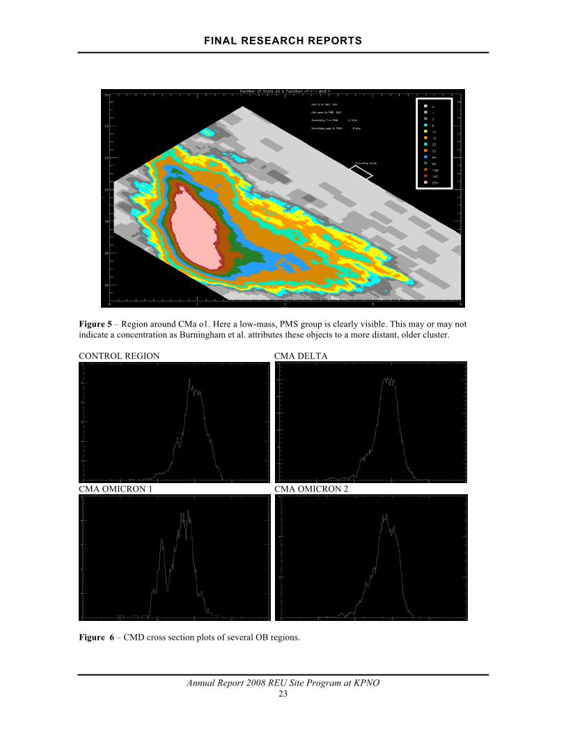
Figure 5 – Region around CMa o1. Here a low-mass, PMS group is clearly visible. This may or may not

indicate a concentration as Burningham et al. attributes these objects to a more distant, older cluster.

CONTROL REGION CMA DELTA

CMA OMICRON 1 CMA OMICRON 2

Figure 6 – CMD cross section plots of several OB regions.



Figure 3 – CMD of the region around CMa �. No clear divide is visible between the main sequence and a

possible low-mass group.

Figure 4 – Smooth CMD of the same region.



Figure 1 – CMD (V-I color plotted against V magnitude) of control fields chosen because they lack a

significant population of low-mass, pre-main sequence stars

Figure 2 – Smooth CMD of the same control fields. Color is assigned based on a number of counts in

rectangular bins



PROJECT

50 fields (13.5 square-arcminutes), including controls, were chosen around several of the brighter stars that de

Zeeuw et al. identified as members of the Cr 121 OB association. VI photometry was performed on each of

the regions and color-magnitude diagrams were made. From the earlier work done on the Orion OB group, it

was clear that a well-defined locus of PMS stars should be visibly separate from the main sequence and

foreground stars. Smooth color-magnitude diagrams were also compiled (see figure) and cross-sections

plotted. These were examined for the possible presence of a concentrated group of young, low-mass stars.

Part of this project also involved writing IDL software to perform matching routines on smaller fields and compiling them into the larger target regions around the association stars. Repeated objects from overlapping

fields as well as concentric long and short exposures were matched through the IDL routine based on their

coordinates, and magnitude values were averaged based on their relative error. The software then created

master catalogues from all of the adjacent and overlapping fields and containing all of the unique objects in

each of the regions (approx 25,000-30,000 objects)

ANALYSIS & RESULTS

The diagrams produced fail to indicate a strong PMS locus around the O and B association stars in Collinder

121. A strong low-mass population was apparent in the vicinity of CMa o1 (See figure), but results from Burningham et al. (2003) indicate that this may be a much more distant cluster of stars along the line of sight

of the moving group de Zeeuw has identified. Diagram features indicate the possibility of a much weaker

PMS concentration than in Orion OB1, which will hopefully encourage further examination of this region and

further inquiry into the nature of OB associations.

The possibility of any concentration around the OB association stars of Cr 121 make it an interesting spot to

test new methods of detecting more sparsely distributed groups of PMS stars. Despite the absence of strong

low-mass populations apparent in the magnitude diagrams, faint features may indicate that the clustering

observed in Orion is indeed present in Canis Major and may, in fact, be an important evolutionary feature of

these young groups.

ACKNOWLEDGEMENT

Special thanks to Dr. Bill Sherry of NOAO for being an excellent mentor and providing invaluable advice

throughout this project.

REFERENCES

Burningham B., Naylor T., Jeffries R., Devey C., 2003, arxiv:astro-ph/0308488v1

de Zeeuw P.T., Hoogerwerf R., de Bruijne J.H.J., Brown A.G.A., Blaauw A., 1999, AJ, 117, 354

Kaltcheva N., Makarov V., 2007, arxiv:astro-ph/0708.3382v1

Sherry W.H., 2003, PhD Thesis, State University of New York, Stony Brook

Sherry W.H., Wolk S.J., 2004, arxiv:astro-ph/0410244v1



Collinder 121: Analyzing its Pre-Main Sequence Population

Matt Henderson

KPNO REU 2008 and Clemson University

Advisor: Dr. William Sherry (NSO)

ABSTRACT

We present a VI photometric census of the regions surrounding some of the stars identified by

de Zeeuw et al. (1999) to be part of an OB association in Canis Major. Studies of Orion OB1

concluded that low-mass, pre-main sequence stars are not uniformly distributed throughout the

association but are concentrated in the regions around the O and B type stars that make up the

group. This study was meant to determine whether this spatial pattern extends to other OB

associations in the solar neighborhood.

INTRODUCTION

Collinder 121 was catalogued as an open cluster at a distance of roughly 1200 pc in 1931. From these early

observations, further attempts were inspired to isolate the population of this group and characterize its

members. de Zeeuw et al. (1999) used astrometry, HIPPARCOS proper motions, to redefine Cr 121 as an OB

association of approximately 100 stars at a distance of 760 pc.

OB associations represent excellent opportunities to study the end products of stellar accretion (Sherry 2003).

These diffuse groups of stars, whose lifespans are limited by the dispersive forces that pull them apart as they

move through the galaxy, are thought to be the structures in which the majority of all stars form (Sherry

2003). Because they are very young (less than 10 Myrs) and because the O and B type stars that distinguish

them share space with a number of low-mass stars, OB associations prove to be good testing sites for some of the principles that govern star formation and group structure (de Zeeuw 1999).

This is especially true in Orion OB1. Subgroups in the belt stars in Orion comprise a zoo of stellar groups in

different stages of evolution. Fossil star-forming regions in which gas and dust have cleared exist alongside

areas such as the Orion Nebula where formation and accretion are still taking place (Sherry 2003). Study of

this region, notably Orion OB1b, a young fossil star-forming group, has discovered some interesting

characteristics of the distribution of low-mass stars within the Orion group. The low-mass, pre-main sequence

(PMS) stars are not evenly distributed throughout the associated but form concentrated groups centered

around their larger, brighter counterparts. Investigating other OB associating within the solar neighborhood to

see if this phenomenon holds true served as the inspiration for this project.



topographies around other parts of the mountain are not particularly the same as El Peñón, the

relationship could be due to a larger scale weather pattern in which case the placement of the service

building does not matter. As can be seen, further investigation into this matter is necessary.

Table 1 - Polynomial Fit Coefficients

a b c d e f g R2

All

Data 3.1214E-07 -2.4253E-05 6.8994E-04 -8.6600E-03 4.5195E-02 -7.4277E-02 9.1262E-01 0.88

< 5 m/s 3.7373E-07 -2.8312E-05 7.8699E-04 -9.6749E-03 4.9614E-02 -8.1753E-02 9.2335E-01 0.83

< 4 m/s 3.0297E-07 -2.2798E-05 6.2271E-04 -7.3605E-03 3.4429E-02 -4.5444E-02 9.2532E-01 0.83

< 3 m/s 2.4387E-07 -1.8506E-05 5.0578E-04 -5.9005E-03 2.6450E-02 -3.2284E-02 9.3884E-01 0.82

< 2 m/s 2.0475E-07 -1.6188E-05 4.6097E-04 -5.6784E-03 2.8563E-02 -5.0756E-02 9.5522E-01 0.82

Average 2.8749E-07 -2.2011E-05 6.1328E-04 -7.4549E-03 3.6850E-02 -5.6903E-02 9.3107E-01 0.84

St. Dev. 6.5256E-08 4.7839E-06 1.3313E-04 1.7293E-03 1.0189E-02 2.0583E-02 1.6406E-02

Polynomial Form: y = ax6 + bx

5 + cx4 + dx

3 + ex2 + fx + g

Table 1 – Coefficients of the 6th order polynomial that was fit to the different plots of lognormal fit m

for seeing as a function of azimuth sector. It can be seen that each of the fits displays very similar coefficients implying an extremely similar shaped curve for each speed cut on the data. The

implications of this are described in Section 4.3.

Acknowledgements

The author would like to thank Dr. Chuck Claver and Dr. Jacques Sebag for useful encouragement, support, and advice throughout the project. In addition, the LSST Corporation, the NSF funded REU

program, and Dr. Chuck Claver are to be given warm thanks for facilitating the associated trip to Cerro

Tololo Inter-American Observatory in Chile to observe star clusters for LSST photometric calibration. Finally, Dr. Ken Mighell and the Kitt Peak National Observatory REU program are to be thanked for

making this project possible.

REFERENCES

Ivezic, Z. et al. 2008, arXiv:0805.2366v1

Sarazin, M. & Roddier F. 1990, A&A, 227, 294-300Sebag, J. et al. 2006, SPIE, 6267-57

Tokovinin, A. 2002, PASP, 114, 1156-1166



Fig. 9a,b – Seeing histograms with least squares lognormal fits for the central sectors in the two most

prominent wind directions. The lognormal fit parameters for the north, north-east direction (left) are

m = 0.875”, s = 0.054” and for the south, south-east direction (right) are m = 0.774”, s = 0.027”.

Fig. 10 – A plot of lognormal parameters m and s for the seeing histogram fits as a function of wind

direction as measured by Sensor 4. The horizontal dotted line is the average of m. As can be seen, both

the best seeing and least spread in the lognormal fit occur when the wind direction is coming out of the

south.

4.3. Discussion

As a result of the analysis presented in Section 4.2, it can safely be determined that the placement of

the service building around the telescope dome will need to be carefully reviewed. Since it is

determined that a large fraction of the wind occurrences (~25%) come out of the direction which is

shown to yield below average seeing, it is important that an artificial structure does not ruin any natural good seeing that occurs. The service building is currently placed in the direction of this flow, and its

placement will need to be reconsidered. However, it is also important to note that the amount of data

that suggests this reconsideration is sparse, and a larger and more complete data set is necessary. Data taken over several seasonal cycles is necessary to determine if the relationship shown in Fig. 10 is

seasonal or constant. In addition, DIMMs and other weather tools placed at other locations on Cerro

Pachón (i.e. those located at Gemini South and SOAR) should be considered so as to determine if the

relationship shown in Fig. 10 holds at other locations around the mountain. If this is the case, since the



Fig. 8a,b,c – Histograms for d as measured by Sensor 4 for October, February, and March respectively

showing the seasonal changes between wind direction. This is important because the best seeing occurs

when the wind is out of the south, which becomes more common when moving from the Chilean

spring to summer to fall.

To take a closer look at items 1 and 2 discussed above, we combine all of the matching seeing and

wind data points for all months into a single comprehensive data set. We then take this data set and

divide it up into 24 x 15 degree sectors based on the d value as measured by Sensor 4. For each azimuth sector, we then plot a histogram of the seeing values and fit the histogram with a least squares

lognormal model with the lognormal parameters mean m and standard deviation s. Fig. 9 shows the

histograms with their respective lognormal parameters for the central sector of each of the two prominent wind directions. Once this has been done for all 24 sectors, m and s can be plotted as a

function of azimuth. This will give a superior indication as to what wind directions give the best

seeing. In Fig. 10, we can see that this plot shows that the below average (best) seeing occurs when the

wind is out of the south. This is significant because over the 7 month time period examined here, 24.99% of the occurrences fall into this category. Fortunately, the sectors which display above average

seeing only consist of 6.01% of occurrences.

It is important to see if this relationship between seeing and wind direction holds for different wind

speed cuts. It is plausible that the DIMM measures the seeing incorrectly when its enclosure is shaken

by high wind. If this is the case, then the relationship shown in Fig. 10 could be shown to be inaccurate. In addition, if exceptionally high winds cause bad seeing, the seeing when the wind comes

out of the north would seem to have much worse seeing since high winds occur mainly from the north.

If the relationship in Fig. 10 disappears at different wind cuts, then it is important to figure out what

percentage of measurements are above the wind cut when the relationship ceases to exist so as to determine the amount of time LSST can expect bad seeing. Finally, if the relationship continues to

exist for all wind speed cuts, it is possible that that the cause of the relationship is not due to the

topography of El Peñón, but to some larger scale weather pattern that could be visible on Cerro Pachón’s entire ridge line. The wind speed was cut at 1 m/s intervals from 5 to 2 m/s. For each cut data

set, we plot a similar graph to Fig. 10. When comparing the cut data set’s plots to the original, we find

that the relationship does indeed hold! As a comparison, we fit all of the plots with a 6th order

polynomial. The coefficients of the polynomial fits are shown in Table 1 to illustrate the similarities between the relationships for all wind speed cuts.



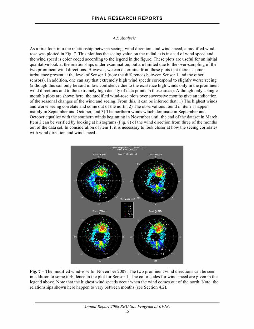
4.2. Analysis

As a first look into the relationship between seeing, wind direction, and wind speed, a modified wind-rose was plotted in Fig. 7. This plot has the seeing value on the radial axis instead of wind speed and

the wind speed is color coded according to the legend in the figure. These plots are useful for an initial

qualitative look at the relationships under examination, but are limited due to the over-sampling of the

two prominent wind directions. However, we can determine from these plots that there is some turbulence present at the level of Sensor 1 (note the differences between Sensor 1 and the other

sensors). In addition, one can say that extremely high wind speeds correspond to slightly worse seeing

(although this can only be said in low confidence due to the existence high winds only in the prominent wind directions and to the extremely high density of data points in those areas). Although only a single

month’s plots are shown here, the modified wind-rose plots over successive months give an indication

of the seasonal changes of the wind and seeing. From this, it can be inferred that: 1) The highest winds

and worse seeing correlate and come out of the north, 2) The observations found in item 1 happen mainly in September and October, and 3) The northern winds which dominate in September and

October equalize with the southern winds beginning in November until the end of the dataset in March.

Item 3 can be verified by looking at histograms (Fig. 8) of the wind direction from three of the months out of the data set. In consideration of item 1, it is necessary to look closer at how the seeing correlates

with wind direction and wind speed.

Fig. 7 – The modified wind-rose for November 2007. The two prominent wind directions can be seen in addition to some turbulence in the plot for Sensor 1. The color codes for wind speed are given in the

legend above. Note that the highest wind speeds occur when the wind comes out of the north. Note: the

relationships shown here happen to vary between months (see Section 4.2).



4. The Correlation between Seeing & Wind

4.1 The Site Layout

As briefly discussed in Section 1, Fig. 1 shows the layout of the components of the LSST on El Peñón.

With the wind-rose of Fig. 2 in mind, note the markings on Fig. 1 indicating the directions of the two

most prominent winds. In addition, the areas of best seeing and worst seeing have been marked. Note that the current design of the summit places the service building facing the South, South-East (in the

direction of the second most prominent wind direction and the area of best seeing). The motivation for

the placement of this building is so that the building can mimic the natural streamline of the mountain. The aim of the following analysis is to characterize the relationship between seeing, wind direction,

and wind speed. The determination of the azimuth sectors with best and worst seeing (as marked on

Figs. 1 and 2) will be explained and it will be determined if the placement of the service building

should be reconsidered so as to not chance disturbing any natural good seeing that may exist when the wind flow is out of a given direction.

Fig. 5a,b,c – 2-D image histogram for z with Sensor 4 as a reference for April 2008. Note the tightness

of the correlation as we move up the tower from the plot on the left to the plot on the right.

Fig. 6a,b,c – 2-D image histogram for d with Sensor 4 as a reference for April 2008. Note the deformation in the correlation of the plot for Sensor 1 and the increasing tightness of the correlation as

we move up the tower from the plot on the left to the plot on the right.



3.3. Discussion

Since the correlations (with Sensor 4 as a reference) of Sensor 1 and 2 are poor with a significant improvement as we travel up the tower to Sensor 3, it has been qualitatively determined that the bulk

of the boundary layer is below Sensor 3 (i.e. below 20m). As such, the predetermined telescope

elevation axis height of 20.5m is verified and will stand unchanged until further analysis. Future work

in this realm will be carried out on the wind tower by replacing the anemometers with micro-thermal sensors. These sensors will be placed at a much finer resolution (with 2m spacing between sensors)

from ground level up to 30m. Although the micro-thermal experiment was intended to be carried out in

this examination to supplement the above qualitative analysis, it was made impossible by an unfortunate collapse of the wind tower in May. The tower has since been reconstructed and this

experiment will be carried out in the near future.

Fig. 4a,b,c – 2-D image histogram for v with Sensor 4 as a reference for September 2007. Note the tightness of the correlation as we move up the tower from the plot on the left to the plot on the right.

Fig. 3a,b,c – Cumulative Distributions

for the month of September 2007. Note

the deviations of the curves for Sensor 1 and 2 from that of 3 and 4 in almost

all cases, indicating the presence of

turbulence at the lower levels.

PROGRAM ACTIVITIES


During analyses when the wind and seeing are to be correlated, those wind data points that have no

matching time stamp in the seeing data set are ignored (note that the time stamps are recorded to an accuracy of one second). Throughout this analysis, MATLAB will be the main facility for data processing

and plotting.

3. Evidence of the Turbulent Boundary Layer

3.1. Simulated Boundary Layer

Computer simulations of turbulence considering the North-South cross-section of El Peñón (which is the direction of most of the wind flow, as we will see below) show that the boundary layer extends to

approximately 100m above the summit. However, at 30m (i.e. the top of the tower), the attenuation of the

input wind is only ~6%. Thus, we assume that Sensor 4 is in near laminar flow.

3.2. Analysis

To begin, we plot a wind-rose (Fig. 2) based on the data

from Sensor 4 for the time period under consideration

(see Section 2) in its entirety. The data points shown on

this wind-rose are only those which have a corresponding seeing data point. This was done only to

reduce the total number of data points since plotting

them all would result in an illegible plot. This gives a basic indication as to where the winds are generally

distributed in near laminar flow. We find that the most

prominent winds come from the North, North-East

(62.31% of all occurrences) and a secondary prominent wind comes from the South, South-East (20.74% of all

occurrences). Most of the wind is under 10 m/s, with the

majority falling under 5 m/s. The highest winds come out of the North, North-East. A brief look at a

cumulative distribution (Fig. 3) of v, z, and d

respectively shows signs of turbulence below Sensor 3. Sensor 3 and 4 are nearly identical when viewed

in this fashion while Sensors 1 and 2 typically

deviate in their own respective ways. Although Fig.

3 is for an individual month only, the observed relationships hold throughout all months examined

in this analysis.

More compelling evidence for turbulence below Sensor 3 is a set of 2-D image histograms. Due to the

exceptionally large number of data points in our sample, a simple scatter plot is useless due to the

inability to make out structure in the relationship between two variables. Instead, we plot a 2-Dhistogram of the scatter plot and display it as an image with each data bin representing a single pixel

and displayed on a log scale. If we are measuring laminar flow, each wind sensor should read the same

value and a scatter plot (here, the 2-D histogram) should show a near perfect correlation. As laminar

flow degrades, one should observe this correlation become poorer, and this is what we observe in these plots. Using Sensor 4 as a reference, Figs. 4-6 show image plots for v, z, and d respectively. Each of

these plots shows that the laminar flow is disturbed at Sensor 1 and Sensor2 with Sensor 3 displaying a

very good correlation. Although Figs. 4-6 are for an individual month only, the observed relationships hold throughout all months examined in this analysis.

Fig. 2 – Wind-rose plot showing the relationship

between wind direction and speed. The colored cones are as described in Fig. 1.

PROGRAM ACTIVITIES


Fig. 1 – LSST site layout on El Peñón. The colored cones represent wind directions with the

indicated characteristics (see Sections 3.2 and 4.2 for descriptions). Note the rectangular

service building extending to the south-west away from the dome.

Cerro Pachón is already known to be a good site overall. While large scale characteristics are known, it is

important to understand characteristics that are local to El Peñón and how the local environment will affect the LSST. The height of the turbulent boundary layer must be determined so as to verify the height

at which the 8.4m telescope will be placed. Currently, LSST's design places the elevation axis of the

telescope at 20.5m. It is necessary to verify that this height is above the boundary layer so as to minimize the degradation and scintillation of starlight due to the atmospheric turbulence that is present at low

heights. To determine this height, wind data at four heights between 5m and 29m will be utilized. In

addition to examining the height of the boundary layer, a mixture of wind and seeing data (which is

measured with a DIMM on the site) will be used to determine if there is any range of wind direction values that display a bias towards below average seeing. This information will help guide the placement

of a service building at a position around the dome so as to not disturb preexisting laminar flow that

allows good seeing (see Fig. 1 for a layout of the site). A description of the methods used to analyze these data, verification for the height for the telescope, and suggestions regarding the placement of the service

building will be described below. In addition, future site characterization techniques related to this project

will be briefly discussed.

2. Equipment & Data

The site characterization presented here will utilize data from two sources on El Peñón: a DIMM and a tower

equipped with anemometers. The DIMM, which is placed near the wind tower, records the Full-Width at Half Maximum (FWHM) seeing on average once every minute and was recorded from September 2007 to March 2008.

The details on how a DIMM calculates the FWHM seeing can be found in Sarazin & Roddier (1990) and Tokovinin

(2002). The tower is equipped with four Metek33 USA-1 Ultrasonic Anemometers, each located at four different

heights and named as follows: Sensor 1 = 5m, Sensor 2 = 12m, Sensor 3 = 20m, and Sensor 4 = 29m. Each

anemometer produces four data parameters: horizontal wind speed (v), vertical wind speed (z), azimuth wind

direction (d), and temperature (t). The data were recorded once per second from August 2007 to April 2008.

3 http://www.metek.de

PROGRAM ACTIVITIES


Site Characterization of El Peñón:

Site of the Large Synoptic Survey Telescope

Taylor S. Chonis

KPNO REU 2008 and University of Nebraska – Lincoln

Advisors: Dr. Chuck F. Claver NOAO) & Dr. Jacques Sebag (NOAO)

ABSTRACT

The Large Synoptic Survey Telescope (LSST), a new 8.4m telescope that will augment and revolutionize

today's arsenal of astronomical survey telescopes, has chosen El Peñón, a peak on Cerro Pachón in

northern Chile, as its site. The LSST is a temporal imaging survey whose productivity and data quality are

a strong function of the characteristics of the site. In an effort to select the site, several years of data for site evaluation were taken at the top four candidate sites. Upon the selection of El Peñón, additional

extensive data has been taken with a differential image motion monitor (DIMM), a weather station, and a

30m tower equipped with four anemometers at different heights. This summary will describe the initial characterization which will be used in an effort to determine the height of the turbulent boundary layer

(above which the telescope must be placed) and to determine if there is a bias towards specific wind

directions with above average seeing (this information will guide the placement of the LSST service

building around the telescope dome).

1. Introduction

The Large Synoptic Survey Telescope1 is a dedicated 8.4m, f/1.25 telescope equipped with a 3.2 Gpixel,

64cm flat imaging surface that will image a 9.62 square degree area on the sky. The LSST project is a revolutionary sky survey that will for the first time survey the sky temporally and spatially every four

days. It is currently scheduled for first-light in 2014. An in depth description can be found in Ivezic et al.

(2008).

It is important to note that for LSST to meet its goals, a high quality site is essential. Since adaptive optics

is not consistent over LSST's large field of view, local site characteristics are extremely important. El

Peñón2, a peak on Cerro Pachón in northern Chile (which is also the site of the SOAR and Gemini South telescopes) was chosen as LSST's site. During site evaluations, two years of data were gathered to support

the selection of El Peñón which included the results of other site campaigns, measurements from existing

infrastructure, all-sky cameras, and weather stations to measure the number of clear nights, seeing characteristics, and sky brightness characteristics for each site (Sebag et al. 2006).

____________________1 http://www.lsst.org2 Selected site information located at http://www.noao.edu/lsst/site

PROGRAM ACTIVITIES


Figure 3 – The weighted wavelet transform as performed on one of the aperiodic variables stars in the BOKS

sample.

Figure 4 – The weighted wavelet transform as performed on one of the aperiodic variables stars in the BOKS

sample.

PROGRAM ACTIVITIES


Figure 1 – The weighted wavelet transform’s results on a simulated, evenly sampled sinusoidal signal. The

transform is the top panel, the original signal the center panel, a best period phase of the data on the bottom left, and

the best period as a function of time on the bottom right.

Figure 2 – A comparison of the effectiveness of the period-finding of the weighted wavelet transform as compared

to the methods used by the authors of the BOKS

PROGRAM ACTIVITIES


5. Results & Conclusion

We then used statistical criteria to select interesting aperiodic variables from our sample. We used light

curves with a large number of points that deviated from the median by a large fraction of their

photometric errors. Using this criterion and the brightness of the object, excluding light curves that suffered from errors in the data reduction process, we obtained on order ten light curves. We additionally

performed tests on different simulated signals that more closely resembled the observational data to

determine if there were artifacts in the wavelet transform that were a result of the observational cadence or the nights removed due to poor observing conditions. Some examples of results of the transform on

aperiodic data are shown in Figures 3 and 4.

The transforms on the aperiodic variables were compared to the results of some transforms on purely

random data. The transforms show a magnitude in the wavelet transform that is orders of magnitude less

than the amplitude evident when the algorithm detects a periodic signal, even one shrouded in noise and

very weak. Also, some of the strongest signals that appear do so at suspicious periods, i.e. those related to the observational cadence (one day, the length of the observation period, etc.). Some of the wavelet

transforms evidence patterns similar to the transforms of other light curves, which, if the light curves were

uncorrelated, should not be the case; instead, these elements of the transform could be a result of the observational properties. Finally, some of the peaks in the power spectrum appear in regions of the signal

that contain no data, which effects confusion and suspicion.

PROGRAM ACTIVITIES


2. Data

The data were collected in the Burrell-Optical-Kepler Survey (BOKS) and surveyed a 1.25 square degree

field of view inside the Kepler mission field. Data were taken for roughly forty nights, and ~55,000 total

light curves were collected in multiple bands. From the set of all light curves, approximately 30,000 were

in the range 14 < r < 19, and several thousand were variables. A collection of 31 light curves with clearperiods were chosen to test the effectiveness of the code developed for this project, and statistical

methods were used to choose on order 10 bright variable but aperiodic stars that were not adversely

affected by systematic errors in the data reduction process.

3. Methods

Traditional methods of time series analysis include Fourier analysis, which can be represented as a

distribution of power in various frequencies of sinusoidal functions. This is ineffective for periodic

signals with frequencies that vary as a function of time, which can include a great many kinds of signals.

To overcome these limitations, methods were developed that would perform a number of Fourier transforms at various temporal points, effectively recovering the frequency power spectrum at every point

of the signal. The so-called windowed transform is the product of the traditional transform with the

window function, which is translated along the signal. The width of the window naturally affects the achieved resolution of the transform; a window with width of the entire signal would be equivalent to

performing a traditional Fourier transform. Smaller windows give better time resolution, but poorer

frequency resolution; the user must make a compromise and choose.

Wavelet methods offer many advantages over these traditional Fourier methods. A wavelet transform

measures the self-similarity of a signal to a ‘mother’ wavelet, which can take a variety of forms, including

sinusoidal functions that mimic more familiar Fourier methods. The ability of the wavelet transform to take any functional form allows for more effective analyses suited for particular searches. Additionally,

the wavelet methods overcome the time-frequency resolution issues. Rather than using basis functions of

different frequencies, the mother wavelet is scaled and translated and the ‘window,’ akin to the window in windowed Fourier transforms, changes its size based on the scaling of the wavelet, so that appropriate

window sizes are used for the particular scaling of the mother wavelet.

To implement the weighted wavelet projection algorithm as shown in Foster 1996, we developed a C code.

4. Tests

We tested the ability of the code to recover periods with various input signals. Different periodic signals

were tested (sinusoidal, sawtooth, step functions, a sum of sinusoidal curves with two different frequencies, etc.) We observed the magnitude of the power in various parts of the transform, and noted

how well it performed at recovering the desired period of the signal. We introduced noise and typical

observational cadences to the signals. We created signals that only existed for brief periods in the entire

observational time, and we noted the response of the transform to a purely random signal. See Figure 1 below for an example of a simulated signal and its weighted wavelet transform. In the Figure, the top plot

is the transform, the middle plot is the original signal with model signals superimposed, the bottom left is

a phased plot of the data with the best period, and the right plot is the best found period as a function of time. After testing the transform on various simulated data, we tested the 31 objects from BOKS that had

known periods. The success of the method was evident, especially since we were not altogether

concerned about the codes’ performance on periodics, but rather aperiodics. Figure 2 shows the comparison of the BOKS period determination with the best period as found by the Foster wavelet

transform.

PROGRAM ACTIVITIES


A Wavelet Time Series Analysis of Aperiodic Variable Stars in the Kepler Field

Timothy Arnold

KPNO REU 2008 and The Ohio State University

Advisors: Kenneth Mighell (NOAO) and Steve Howell (NOAO)

Abstract. The temporally varying sky offers insights into physical mechanisms and can be used as a

useful tool for many other purposes, e.g. as standard candles. Periodic variables have been the simplest to classify, understand, and use, but many variable light curves are discarded due to their apparent

uselessness as aperiodic. Many contemporary projects (e.g. the Large Synoptic Survey Telescope,

PanSTARRS, the Kepler mission) aim to map the transient sky, and methods of time analysis have become more advanced; it would be advantageous to discover identifying information in these discarded

light curves. We use a wavelet analysis, based on a weighted projection on basis functions, to analyze

aperiodic variable stars in the Burrell-Optical-Kepler Survey (BOKS). Using the Weighted Wavelet Z-Transform detailed in Foster 1996, we find that variable but aperiodic stars in our sample offer little

characteristic properties for further classification.

1. Introduction

The pursuit of scientists is to measure regularities in the way nature behaves. Studying signals or phenomenon that vary in a periodic—regular—fashion is in the same tradition as the fundamental

activities of scientists. Time analysis techniques have grown and become more advanced with the

increasing need for them as scientists discover that irregularly and chaotically evolving systems are the

norm rather than the exception. Traditional Fourier methods have been expanded to windowed transforms, sampling small portions of the signal to analyze and gaining an understanding of the

frequency power spectrum as a function of time instead of from the entire signal. Wavelet analysis has

been developed to overcome many of the shortcomings of time-frequency Fourier analysis; we implement an algorithm based on a weighted wavelet projection technique to effectively analyze poorly sampled

astronomical light curves.

Variable objects have been extremely useful for astronomers to identify physical mechanisms and

discover new types of objects. These objects come in many varieties, some acting periodically on a wide

variety of time scales (pulsating stars, pulsars), others one-time events (supernovae, microlensing events,

gamma ray bursts), and still others some mixture of the two (single events that repeat on uncertain time scales—novae, e.g.). Unfortunately for astronomers attempting to analyze astronomical time series, the

data are often plagued with irregular spacing and sporadic omissions, due to observational cadences or

poor weather. Few projects have the luxury of multiple observing sites to collect continuous and well-sampled data. For this reason, weighted wavelet projection methods were used, which overcome many of

the unreliable results of traditional time-series transforms on nonideal data.

PROGRAM ACTIVITIES


• Buell Jannuzi (KPNO Director), “Welcome to the National Optical Astronomy Observatory”

• Dick Shaw (NOAO): "Planetary Nebulae in the Magellanic Clouds: Clues to Stellar Evolution"

• Rachel Howe (NSO), “Introduction to Helioseismology”

• Frank Hill (NSO): “Solar Magnetic Fields”

• Marianne Faurobert (University of Nice): “Measuring Line Formation Depths by Interspectral

Analysis”

• Claude Aime (University of Nice): “Use of an Apodized Aperture for Solar Coronagraphy”

• Steve Kiehl (NSO): “The Advanced Technology Solar Telescope”

• Liz Alverez (NOAO): “Site Protection and Light Pollution”

• Jennifer Lotz (NOAO): “Collisions in the Cosmos”

• Mike Merrill (NOAO): “Introduction to Infrared Astrophysics”

• Daniel Harbeck (WIYN): “The WIYN One Degree Imager Project”

• Chuck Claver (NOAO/LSST): “The Large Synoptic Survey Telescope”

• Jim Liebert (University of Arizona): “The Astrophysics Graduate School Admission Process”

PROGRAM ACTIVITIES


Research Projects

The summer 2008 REU students at KPNO spent an average of 11 weeks working as full-time research assistants on projects ranging from the analysis of stellar open clusters, a study of galaxy

mergers, to the site characterization of El Peñón (the proposed site of the LSST). In addition to

work on their individual projects, the students collaborated in designing observational programs

carried out at the KPNO 2.1-m telescopes during 14 nights of observing in July 2008 (an average of 5 observing nights per student). The observational projects are an essential feature of the KPNO

program, allowing each of the students to experience first hand the process of designing and

carrying out an original observing program at the national observatory.

Towards the end of the program, REU students are required to share their research findings with the

NOAO astronomical community through oral presentations and written reports. For many of the

students, this was their first experience presenting research results in a professional scientific

setting. The titles of the students’ research topics, presentations, and written reports are listed

below. The original written reports are presented in the following section.

•Timothy Arnold: A Wavelet Time Series Analysis of Aperiodic Variable Stars in the Kepler Field

•Taylor S. Chonis: Site Characterization of El Peñón:Site of the Large Synoptic Survey Telescope

•Matt Henderson: Collinder 121: Analyzing its Pre-Main Sequence Population

•Tiffany Meshkat: Deep Photometry of the Open Cluster IC4651

•Ashley Stewart: Analyzing the Effects of Scattered Light on Stellar Photometry

•Matthew Zagursky: Investigating Galaxy Mergers with IGNITE

Scientific Lectures and Field Trips

In addition to the research project, two popular components of the KPNO REU program are the

weekly science lectures given by NOAO staff and the field trips to nearby observatories and non-

NOAO facilities. The lectures and field trips are designed to introduce the REU students to a broad

array of current scientific topics—including instrumentation issues—in O/IR ground-based, space-

based, and radio astronomy. The KPNO and NSO REU students visited the National Solar

Observatory facilities at Sacramento Peak, New Mexico, during July 9 – 12, 2008; they toured the

nearby Apache Point Observatory, and were also given a custom tour of NRAO’s Very Large

Array. Our lecture speakers included NOAO and NSO directors, astronomers, and scientists. The

KPNO REU lectures are informal which allows the students to interact and network with scientists

working in many different areas of ground-based & space-based astronomy, solar astronomy, and

instrumentation. The topics of the 2008 REU lecture series (June 9 – August 5, 2008) are listed on

the next page.

PROGRAM ACTIVITIES


Recruitment

Last year, we had a total of 138 complete and 21 incomplete applicants to our program. From the

138 qualified applicants, six undergraduate students (two women and four men, none from under-represented minorities) were selected to participate in the 2008 REU site program at KPNO. About

four months before the application deadline, NOAO began recruitment for the program via

announcements on the KPNO REU web site (http://www.noao.edu/kpno/reu/), and by posters and

letters sent to colleges and universities across the US and Puerto Rico. In October 2007, approximately 900 posters and letters were mailed to US college and university Science Department

chairs and undergraduate advisors (principally in physics, astronomy, math, computer science, and

engineering programs); as well as to campus job placement and career counseling offices. Our 138 applicants attended 115 schools in 37 states; 49.0% of applicants were women (70 out of 159; 16 gave

no gender) and 51.0% were men (73 out of 146). Of the 137 applicants who gave information about

their race, we had 6 who classified themselves as African-American (4.4%), 7 as Hispanic (5.1%), 7

as Mixed/Other (5.1%), 8 as Asian (5.8%), and 109 as Caucasian (79.6%). Of the 153 applicants who gave information about where they heard about the KPNO REU program, 6 said from previous

REU students (3.9%), 19 said their advisor (12.4%), 20 said college or department staff member

(13.1%), 18 said the REU poster on a bulletin board (11.8%), 87 said the KPNO REU Web site (56.8%), 1 learned of the program in a journal (0.7%), and 2 said “other” (1.3%).

Participants

Each of the students selected for the program

was matched with an NOAO scientific staff

member to work on a research project previously proposed by them and evaluated by

the REU site director. In general, the scientific

projects most likely to be approved for the

program are those that provide the greatest opportunity for the REU assistant to make

substantial progress over the course of the

summer, as well as those likely to result in an eventual scientific publication in which the

student is a collaborator. Particular research

topics are assigned to particular students in

consideration of the student’s background and avowed scientific interests (as expressed in the

student’s application)

The six REU students, their college/university affiliations, and the NOAO scientists designated as their research advisors for the program are listed as follows:

REU Participant College/University NOAO Research Advisor(s)

Timothy Arnold Ohio State University S. Howell, K. Mighell, & K. Garmany

Taylor Chonis University of Nebraska, Lincoln C. Claver & J. Sebag

Matthew Henderson Clemson University B. Sherry

Tiffany Meshkat University of California, Los Angeles C. Claver & K. Mighell

Ashely Stewart University of Arkansas J. Glaspey

Matthew Zagursky University of Maryland J. Lotz

Left to right: Taylor Chonis, Matthew Henderson,

Ashley Stewart, Matthew Zagursky, Tiffany

Meshkat, Tim Arnold.

PROJECT SUMMARY


The National Science Foundation Research Experiences for

Undergraduates (REU) program is designed to encourage US college

and university students to pursue careers in science and engineering.

REU site programs make it possible for undergraduates to take part in

independent research activities with professional scientists at major

research institutions, usually during the summer months. Every year

since 1990, NSF has awarded funding to the National Optical

Astronomy Observatory (NOAO) to support an REU site program in

astronomy at Kitt Peak National Observatory (KPNO).

Six undergraduates were hired as full-time employees at NOAO in Tucson for a period of ten to

eleven weeks, beginning at the end of May 2008, with the $80,371 allocated to the 2008 KPNO REU

program. The students spent the major portion of the program working as research assistants with

designated members of the NOAO scientific staff (REU “mentors”) on independent, supervised

research projects. In the past, former KPNO REU participants have noted that the chance to attend

and participate at a major meeting of the American Astronomical Society (AAS) is one of the most

exciting aspects of our REU program. All six of our KPNO REU 2008 participants will be attending

the upcoming 213th AAS meeting which will be held at Long Beach, CA on January 4 – 8, 2009.

While at the AAS meeting, these students will be presenting posters – all as the presenting author. Of

our six participants last year, two were women and four were men. The KPNO REU Site Director for

the 2008 program was Kenneth Mighell.

In addition to work on their particular research projects, the REU students attended weekly science

seminars and lectures by members of the NOAO scientific staff, gave periodic oral reports on the

progress of their research to NOAO and visiting scientists, visited and toured nearby observatories

and research facilities, and planned and executed observing programs using the world-class

optical/infrared telescopes on Kitt Peak. Along with the students of the concurrent REU program at

the National Solar Observatory (NSO) in Tucson, the KPNO students also traveled to Sunspot, New

Mexico, on a four-day field trip to visit the NSO facilities at Sacramento Peak and the National

Radio Astronomy Observatory’s Very Large Array.

At the end of the summer program, the KPNO students were required to write up the results of their

research work as concise and coherent scientific papers. All will appear in print in the Bulletin of the

American Astronomical Society in January 2009. The student papers are presented in this Annual

Report under the section Final Research Reports. The abstracts to be presented at the 213th AAS

meetings are reproduced below under the heading Publications and Products.

TABLE OF CONTENTS

Annual Report 2008 REU Site Program at KPNOi

NSF RESEARCH EXPERIENCES FOR UNDERGRADUATES (REU)

Site Program in Astronomy at the

Kitt Peak National Observatory

D. Silva, Principal Investigator

K. Mighell, Site Director & Co-Principal Investigator

Annual Report for the 2008 REU Program at KPNO

Project Summary ...................................................................................................................................... 1

Program Activities and Participants ........................................................................................................ 2

Final Research Reports ............................................................................................................................ 5

Publications and Products ...................................................................................................................... 44

NATIONAL OPTICAL ASTRONOMY OBSERVATORY

NSF Research Experiences for UndergraduatesSite Program in Astronomy at

Kitt Peak National Observatory (KPNO)

Annual Project Report 2008 (AST 0754223)

Submitted to

Brian M. Patten, Ph.D.

NSF, Program Director for Education and Special Programs

David Silva, Principal Investigator

December 10, 2008

noao newsleter (december 2008) 13 kpno reu 09 annual .pdf · isochrones. white dwarf candidates...

Documents