noise in satellite links - del mar north · noise in satellite links gert cuypers, [email protected]...

Noise in satellite links

Gert Cuypers, [email protected]

Considering the difficulties achieving a terrestrial link, it might be surprising that satellitelinks, covering much greater distance are possible at all. One of the most important factorsto explain this is the noise involved.When signals originate at the satellite, they are virtuallyfree of noise. The origin of noise and the meaning of the noise figure and temperature inrelation to receivers will be explained. The effect of the Earth atmosphere on signal-to-noiseratio (SNR) will be illustrated with a real-life example.

1 Theory

1.1 Thermal noise

Except at absolute zero temperature, the electrons in every conductor (resistor) are alwaysin thermal motion, resulting in a voltage difference between the resistor’s terminals. Thiscan be modeled as a noise source Nth inside the resistor, as shown in figure 1. If the resistor

RR (physical) RkTB

Nth

(ideal) (ideal)

Figure 1: a non-ideal resistor and its equivalent scheme, attached to an amplifier

is connected to a matched ’load’, e.g. the input impedance of an LNA (low noise amplifier),the thermal noise source in the resistor delivers a power to the load, equal to:

N = kTB, (1)

with k the Bolzmann constant(

1, 38.10−23 WK.Hz

)

,T the absolute temperature in Kelvin, andB the bandwidth [Hz].

1

Belgian Microwave roundtable 2001 Noise in Satellite links

Note that the thermal noise power is independent of the resistance value, but proportional tothe resistor temperature. Thus, if one would connect a resistor (dummy load) to a sensitivepower meter, one would notice an increase in noise power when the resistor is heated by e.g.a candle flame!

Because of the simple relation between the noise and the resistor temperature, it issensible to define an effective noise temperature for other noise sources too, even if they arenot thermal in origin, e.g. interference from another station. A noise source having a ’noisetemperature Tn’ generates a noise power, equal to the thermal noise that would be generatedby a resistor at temperature Tn.

It may come as a surprise that resistors exhibit a noisy voltage at their terminals. A verycomparable phenomenon exists for matter, or bodies at a certain temperature: every objector matter that absorbs radiation also produces noise through radiation. Again, this maysound strange at first sight, but after all it is just an extension to ’low’ frequencies, of thecommon observation that hot objects (such as a candle flame) emit visible light. For a perfectabsorbing object or so-called blackbody the emanating noise is proportional to the object’stemperature, and is also given by equation 1. Most of the time, this relation is also a goodapproximation for non-perfectly absorbing objects, such as the Sun for instance. Imagineone would point an antenna towards the Sun, such that it is the only object contained in theantenna bundle. If a power meter is attached to the antenna (as in figure 2), and one wouldlook at the power contained in a bandwidth of e.g. 4kHz, then the readout would be equalto 1, 38.10−23.105.4000 = 5, 5−15Watts = −113 dBm, because the Sun is approximately at105 Kelvin. In case the antenna isn’t directional enough, and the bundle is too wide, thepower measured will be a weighted average of the different bodies the antenna is looking at.

SUN

Power meter

Antenna beam

Figure 2: Measuring the thermal noise emerging from the Sun

1.2 Noise figure and noise temperature

Consider an non-ideal amplifier with gain G, having an input consisting of a useful signal Sin

with some noise Nin. Of course, the signal as well as the noise will be amplified. Moreover,the amplifier will add some extra noise to the signal. Because it is a hard to locate thisstrange noise source in the amplifier, it can be replaced with an ideal amplifier and anartificial noise source Nai at its input, accounting for the noise, induced by the amplifier. Infigure 3, such a setup is shown.

2


GinN

inS

inN

inS Nai G

Figure 3: a non-ideal amplifier and its equivalent scheme

1.2.1 Noise figure

The noise figure F indicates the decrease in signal-to-noise ratio (SNR) between the inputand the output of a system. In other words,

F =SNRin

SNRout

=

(

Sin

Nin

)

(

GSin

G(Nin+Nai)

) =Nin + Nai

Nin

= 1 +Nai

Nin

. (2)

Judging from equation (2), the noise figure is dependent on the noise power at the inputNin. To make it possible to compare different amplifiers, people have to a fixed referencenoise power, equal to the noise generated in a resistor at T0 = 290K. The noise power ofsuch a source at 290K is equal to:

N0 = kT0 = 1, 38.10−23.290 = 4.10−23W/Hz

In practice this means that an ’amplifier having a noise figure of 3 dB’ will have anequivalent noise source Nai at its input, equal to the reference noise source of 4.10−23W/Hz.Indeed, if we look at figure 3, and make Nai equal to Nin, the noise power doubles such thatthe SNR at the output will be 3 dB lower than the SNR at the input, and this is equal tothe noise figure. This artificial noise source Nai can now be thought of as fixed.

1.2.2 Noise temperature

Because these very low noise powers are numerically difficult to deal with, the effective noise

temperature Tai (see also §1.1) of a noise source Nai was defined as:

Tai = (F − 1).T0 = (F − 1).290K (3)

When dealing with terrestrial links only, the noise figure F is the most interesting measureof performance of e.g. preamplifiers, because the incoming source temperature will typicallybe around 290K. In this case, the noise figure effectively indicates the loss in SNR. Whendealing with satellite sources, the source temperature will generally be much lower, such thatthe noise figure becomes misleading. In this case, the effective noise temperature is moreinteresting, because it is independent of any reference. It is very important to note thatthe description of the noise figure as ’the difference in SNR between input and output’ only

3


holds if the source noise is indeed at 290K. When the source noise is much lower, as is oftenthe case in space communications for instance, an amplifier ’having a noise figure of 3 dB’will degrade the SNR much more than 3 dB!

1.2.3 Some examples

Some noise figures of interest are:

• a lossy line at temperature 290K has a noise figure equal to the insertion loss. In otherwords, if the line has a signal loss of 10 dB, the noise figure equals 10 dB as well.

• a cascade of amplifiers, e.g. an LNA and PAs (power amplifiers), such as in figure 4has a composite noise figure equal to:

Fcascade = F1 +F2 − 1

G1+

F3 − 1

G1.G2. . . (4)

G

F

G

F

G

F

1

1

2

2

3

3

(possible trans−mission line)

LNA PA PA

Figure 4: amplifier cascade and their associated noise figure

From this it follows that the first amplifier stage is the most critical and should have thelowest noise figure (F1), and preferably high gain. Moreover, if the chain of amplifiers ispreceded by a transmission line (as is most often the case), this transmission line can beregarded as an ’amplifier’ with a gain lower than unity. Obviously such lines should be keptas short as possible, and preferably avoided (or placed behind the LNA), when dealing withvery weak incoming signals!

Imagine one has to use a long cable, and wants to install a preamp to compensate forthe transmission loss. Suppose the amplifier has G = 30 dB and F = 2 and the line hasan insertion loss of 10 dB. The noise figure of the transmission line is equal to the insertionloss, as stated before, and equals 10 dB. The signal amplification of this system is equal to100 (20 dB), regardless of the configuration. The noise, assuming the amplifier precedes thetransmission line, equals

Famp+line = 2 +10 − 1

1000= 2, 009 ' 3 dB.

If, on the other hand, the line precedes the amplifier, the noise figure is equal to

Fline+amp = 10 +2 − 1

110

= 20 ' 13 dB.

Quite a difference! In both cases, the signal amplification is equal to 20 dB, but the noisefigure is 10 dB’s apart.

4


2 Satellite communications

2.1 Atmospheric absorption

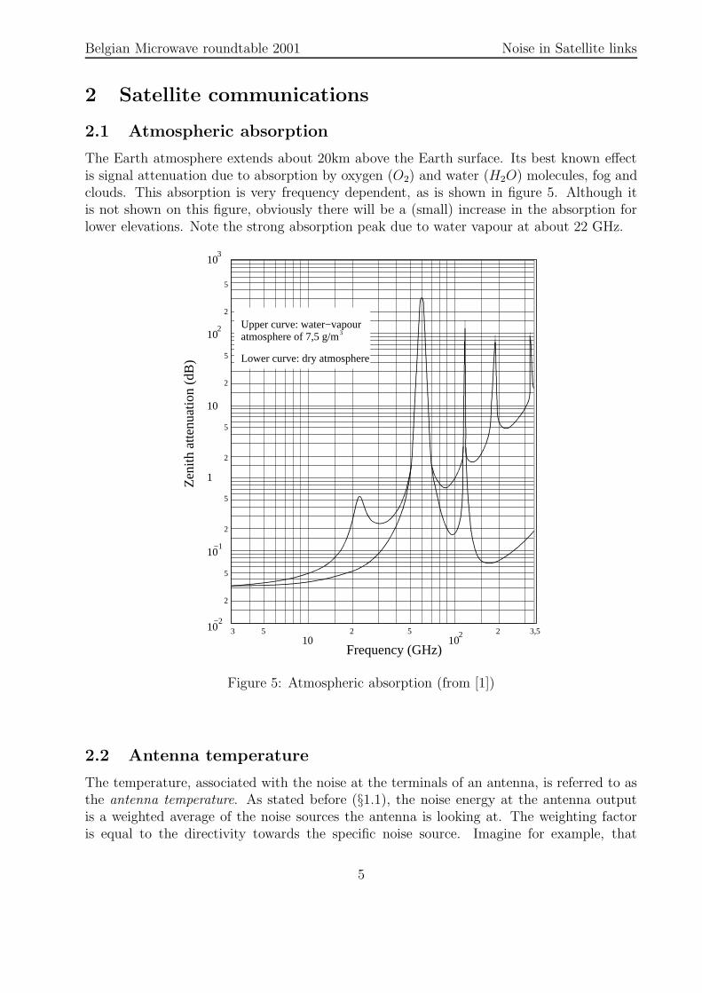
The Earth atmosphere extends about 20km above the Earth surface. Its best known effectis signal attenuation due to absorption by oxygen (O2) and water (H2O) molecules, fog andclouds. This absorption is very frequency dependent, as is shown in figure 5. Although itis not shown on this figure, obviously there will be a (small) increase in the absorption forlower elevations. Note the strong absorption peak due to water vapour at about 22 GHz.

103 5 2 5 2 3,5

5

2

102

Frequency (GHz)

1

10

10

10

3

2

−1

10−2

10

5

2

2

2

2

5

5

5

Zen

ith a

ttenu

atio

n (d

B)

Upper curve: water−vapouratmosphere of 7,5 g/m3

Lower curve: dry atmosphere

Figure 5: Atmospheric absorption (from [1])

2.2 Antenna temperature

The temperature, associated with the noise at the terminals of an antenna, is referred to asthe antenna temperature. As stated before (§1.1), the noise energy at the antenna outputis a weighted average of the noise sources the antenna is looking at. The weighting factoris equal to the directivity towards the specific noise source. Imagine for example, that

5


3K

3K 3K

100K

Figure 6: Antenna temperature in the absence and presence of atmosphere

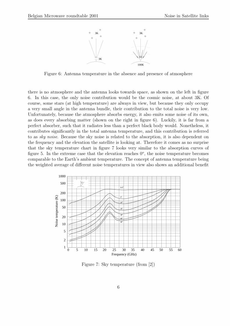
there is no atmosphere and the antenna looks towards space, as shown on the left in figure6. In this case, the only noise contribution would be the cosmic noise, at about 3K. Ofcourse, some stars (at high temperature) are always in view, but because they only occupya very small angle in the antenna bundle, their contribution to the total noise is very low.Unfortunately, because the atmosphere absorbs energy, it also emits some noise of its own,as does every absorbing matter (shown on the right in figure 6). Luckily, it is far from aperfect absorber, such that it radiates less than a perfect black body would. Nonetheless, itcontributes significantly in the total antenna temperature, and this contribution is referredto as sky noise. Because the sky noise is related to the absorption, it is also dependent onthe frequency and the elevation the satellite is looking at. Therefore it comes as no surprisethat the sky temperature chart in figure 7 looks very similar to the absorption curves offigure 5. In the extreme case that the elevation reaches 0o, the noise temperature becomescomparable to the Earth’s ambient temperature. The concept of antenna temperature beingthe weighted average of different noise temperatures in view also shows an additional benefit

θ=

5

50

100

605550454035302520151050

2

1

200

10

2030

90ο

500

1000

Noi

se te

mpe

ratu

re (

K)

Frequency (GHz)

10

20

ο60

5

0ο

ο

ο

ο

ο

θ

Figure 7: Sky temperature (from [2])

6


from the use of directional antennae. Indeed, directivity towards a signal source also impliesa reduced sensitivity in other directions, e.g. the Sun. Man-made noise, emanating frommachinery etc plays little role in frequencies above 1 GHz.

2.3 Effect of rain

The presence of rainfall has a dramatic influence on the link quality, due to absorptionand reflection. Indeed, rain scatter for instance, however useful it may be for terrestriallinks, suggests that a lot of signal doesn’t arrive outside the atmosphere. The absorptionis dependent on the rainfall intensity and on the path length. Figure 8 shows the specificattenuation due to rainfall and the effective path length. The combination of both graphsallows to calculate the attenuation.

Figure 8: Rainfall absorption: specific attenuation and effective path length [3]

Moreover, because of the high absorption, rain also acts as a rather strong noise source.To take this into account, the sky temperature from figure 7 has to be augmented with Train,equal to:

Train = Tm

(

1 −1

Arain

)

, (5)

with Tm the effective temperature of the rain (approximately 260K [3]), andArain the rainfall attenuation

7


2.4 System effective temperature

So far two noise sources have been identified: the antenna noise, being a weighted average ofexternal noise sources, both natural and man-made, and the noise introduced by transmissionlines and the preamplifier. The system effective noise temperature is equal to:

Ts = Ta + Trec, (6)

with Ta the antenna temperature, andTrec the receiver (line+preamp) temperature.

Obviously, low noise amplifiers cannot avoid antenna noise preceding them. Indeed, if aparabolic dish feed has a very wide angle (as in figure 9), the feed itself will not only’look’ towards the dish, but also to the environment behind the dish, at 290K! In satellitecommunications, it is therefore interesting to sacrifice some dish surface to avoid spillover.However, this results in a loss in both efficiency and gain. The tradeoff between gain andantenna noise is best reflected in the figure of merit

G

Ts

,

also called receiver sensitivity.

Spillover 290K

290K

Dish

Feed100K

3K

Figure 9: Antenna noise sources. Note the dramatic effect of spillover

8


3 Example

A realistic link budget will now be evaluated for a satellite downlink at 24 GHz, such as e.g.the Amsat Oscar-40 K-band downlink [4]. Bright and rainy conditions are compared. Wemake the following assumptions:

• The transmitter has Pt = 30 dBm signal power and the transmit antenna gain isGt = 23 dBi (the ’i’ stands for the gain as compared to an isotropic antenna).

• The satellite is worked when it is at its apogee (’highest point’), at about 60000 km,with an elevation θ = 45o. Recall that the free space loss Lfs, i.e. the loss due to thedivergence of the radio waves (without absorption) is calculated as:

Lfs =λ2

(4πd), (7)

with λ the wavelength in meters andd the distance in meters

At 24 GHz, this free space loss is equal to 2, 7.10−22, or −215 dB.

• From figure 5, one can read the atmospheric attenuation at 24 GHz as about 0, 5 dBunder humid conditions.

• The specific attenuation of rain (assume 5mm/h) at 24 GHz can be read from figure 8as about 1 dB/km. The effective path at an elevation θ = 45o is 5 km. This results inan attenuation of 5 dB.

• The increment in antenna noise temperature due to the rain can be calculated usingformula 5 and is equal to Train = 178 K.

• A parabolic dish with a diameter of 45 cm (and thus an area equal to 0, 16m2) is usedfor reception, with an antenna efficiency of 50% (due to the low edge illumination toavoid spillover). The gain of such a dish is equal to:

Gr =4ηπAr

λ2, (8)

with η the antenna efficiency,Ar the (receive) antenna surface (in square meters), andλ the wavelength in meters.

For this example, Gr = 1, 3.104 = 41 dB.

• The sky temperature under bright conditions can be read from figure 6 as about 30K.

• The receiver has a bandwidth of 3 kHz, and a noise figure equal to 3 dBm. Accordingto equation 3, this corresponds to an equivalent noise temperature Trec equal to 290K.For comparison, the link budget will also be calculated assuming a noise figure of 2dB. This corresponds to a noise temperature Trec equal to 170K.

9


No rain RainfallSignal Noise Signal Noise

Transmitter power 30 dBm 30 dBmTransmit antenna gain +23 dB +23 dB

Path loss −215 dB −215 dBSky noise 30 K 208 K

Atmospheric absorption −0, 5 dB −0, 5 dBRainfall absorption −5 dB

Receive antenna gain +41 dB +41 dBReceiver noise temperature 290 K 290 KSystem noise temperature 320 K 498 K

Total power in 3 kHz −121, 5 dBm −138, 8 dBm −126, 5 dBm −136, 9 dBm

Table 1: Example of 24GHz link budget

These figures have been collected in table 3. If no rain is present, the SNR is equal to 17,8dB, which is very comfortable. Although rain only attenuates the signal by 5 dB, it lowersthe SNR to 10,4 dB. Reception with the low-noise receiver (noise figure equal to 2dB) givesrise to SNRs that are respectively 19,7 dB and 11,5 dB. Note that the low-noise receiver ismore beneficial in case of a bright sky (SNR improvement of 1,9 dB) than in case of rain(only 1,1 dB improvement).

References

[1] Recommendation ITU-R PI.676-2:Attenuation by atmospheric gases

[2] Recommendation ITU-R PI.372-6:Radio noise

[3] Satellite Communications Systems, G Maral & M Bousquet, Wiley 1987

[4] http://www.amsat.org/amsat/sats/phase3d/k_tx.html

10

noise in satellite links - del mar north · noise in satellite links gert cuypers, [email protected]...

Documents