noise reduction schemes for chaotic time series

ELSEVIER Physica D 79 (1994) 174-192

PHYSICA

Noise reduction schemes for chaotic time series

Mike Davies Centre for Nonlinear Dynamics, University College London, Gower Street, London WCIE 6BT, UK

Received 29 August 1992; revised 29 November 1993; accepted 6 May 1994 Communicated by A.V. Holden

Abstract

There has recently been a great deal of interest in the development of noise reduction techniques for noisy trajectories from nonlinear dynamical systems. Particular attention has been shown to their development for use in the analysis of chaotic time series. In this paper we consider the problem in an optimisation context. This allows us to categorise some of the commonly used techniques and to compare the performance of different methods from a theoretical standpoint in order to identify some of the pitfalls that can occur with these methods. Finally this formulation enables us to propose a natural composite method that provides flexibility between speed and stability.

1. Introduction

Improvemen t s in t ime series analysis, gained f rom dynamical systems theory, have led to an increased interest in data f rom nonlinear systems with complex dynamics. With the aid of mapping approximat ions and an understanding of the problems of embedding many of the analysis techniques that so far have been restricted to numerical models are now accessible to the experimentalist . However not all experiments can be controlled enough to stop the noise in the system f rom becoming a problem. This has led to a great deal of research being focused upon the p rob lem of reducing noise f rom such data. As in most of the previous work on noise reduction, the noise is assumed to be I . I .D. (Identical Independen t Distribution) and the noise level is assumed to be small with respect to the level of the deterministic signal. Fur thermore the noise

reduction procedure is considered separately f rom the approximat ion of the dynamics. Argu- ments for and against this are considered in Section 2.

In this paper we t reat this p rob lem as a simple minimisation task, adjusting the t ra jectory to minimise the dynamic error. By definition of the te rm noise reduction, this approach seems quite natural. Indeed one of the original noise reduction schemes proposed by Kostelich and Yorke [1] used the idea of minimisation. H o w e v e r the aim there was to adjust the orbit to make it more deterministic while remaining close to the original data. Unfor tunate ly this does not provide a unique minimisation process since it involves simultaneously minimising the distance of the new trajectory f rom the old one and the size of the dynamic error. Thus an arbitrary weight has to be incorporated to balance the two tasks. This is in essence an a priori est imate of the relative

0167-2789/94/$07.00 �9 1994 Elsevier Science B.V. All rights reserved SSDI 0167-2789(94)00136-E

M. Davies / Physica D 79 (1994) 174-192 175

amounts of dynamic and measurement noise present in the data.

Here we will consider the simpler problem of merely minimising the dynamic noise as much as possible. This is not a serious simplification since, if the data comes from a hyperbolic attractor and the noise level is sufficiently small, then we know from Bowen's shadowing Lemma [2] that we can reduce the dynamic error to zero. Fur thermore if the data set is infinitely long then the deterministic orbit is unique. Although we will never encounter an infinitely long trajectory, we will argue that the deterministic orbit for a finite length noisy trajectory is almost unique and is only badly defined at the ends (i.e. little is gained by explicitly minimising the shadowing distance as was proposed in Farmer Sidorowich

[31). If the data did not come from a hyperbolic

attractor, or the noise level is too high to enable shadowing then, as long as the algorithm is forced to be stable it will cease to adjust the data when no further noise reduction is possible (i.e. the cost function will become flat). In the absence of any prior knowledge of the noise this provides a natural replacement for the arbitrary weight used by Kostelich and Yorke.

A further advantage in treating the problem in this way is that many of the previously proposed schemes for noise reduction can be viewed as simple minimisation or root-finding procedures. In general these can be broadly classified as either a Newton based [3,4] or a gradient descent based [5-8] method for minimising, or zeroing the dynamic noise. Hammel [4] and Farmer and Sidorowich [3] explained some of the problems that can occur in using the Newton based approach, particularly those problems associated with homoclinic tangencies and, in Section 3.2, we provide an estimate for the ill-conditioning that these produce. Farmer and Sidorowich demonstra ted that one solution is to use singular value decomposit ion to invert the badly conditioned matrix. However this matrix is banded and will generally have a very low bandwidth, so

it would be preferable to be able to exploit this structure and find a stable order N inversion process as opposed to using singular value decomposition which is order N3! It would also be preferable if manifold decomposit ion [4] (which can be used in the absence of homoclinic tangencies) was not needed. Manifold decomposit ion is not a problem in terms of speed since this is an order N process, however it requires the tangent spaces to be split into stable and unstable directions which is difficult in the presence of tangencies. Fur thermore , if a time series has been samples from a flow, unless it can be reduced to a Poincar6 map, the sampled time series will contain a zero Lyapunov exponent and manifold decomposition will not be applicable.

One possible solution to this problem would ~,c to use a gradient descent method. These are more stable than the Newton methods and work at noise levels that are significantly higher. This is because they do not assume so much about the closeness of the pseudo-orbit and the deterministic shadowing orbit. However once the gradient descent method has been chosen the experimentalist is opting for an algorithm that only converges linearly onto a deterministic orbit. Also some of these algorithms will, in general, not even converge linearly in regions close to homoclinic tangencies [8,9].

Ideally we would like an algorithm that worked for large amounts of noise, whose process is of order N and whose asymptotic convergence is quadratic rather than linear. The composite method presented below appears to achieve all these requirements. The approach used here is a quasi-Newton method (Levenberg -Marquard t method [10]). This is shown to provide a simple and effective solution to the instabilities and convergence problems that are associated with the Newton method and the gradient descent method when they are applied individually.

We conclude the paper with two examples of noise reduction. In the first example we compare the gradient descent, manifold decomposit ion

176 M. Davies / Physica D 79 (1994) 174-192

and Levenberg-Marquard t algorithms when applied to the Hdnon map with knowledge of the dynamics. Finally we apply gradient descent and Levenberg-Marquard t algorithms to data taken from the Lorenz equation. Here the dynamics has to be approximated and it is clear that this provides the main limitation to the effectiveness of the noise reduction algorithm.

2. Function approximation and noise reduction

When the dynamics are not known a priori and we are merely presented with a scalar time series it is necessary to initially embed the data in a reconstructed state space. From Takens ' theorem, [11], we know that we can achieve this using delay vectors. Fur thermore these can be generalised to combinations of linearly filtered delay coordinates (see [12-14]). For a detailed discussion of optimising the embedding we refer the reader to Casdagli et al. [15].

Once the data has been embedded we can model the dynamics by fitting a function to map points forward in time (although this is the general approach, Schrieber and Grassberger use a non-predictive function). There are a variety of methods for approximating the mapping function both locally, [16], or globally, [17], however the basic idea is the same in each case. Having defined a space of functions, we wish to choose the function that best approximates the dynamics. General ly this means minimising the errors, in a least squared sense, where the error terms

are defined as:

= x , - (1)

where e i is the approximation error associated with xg the ith point in the series and f is the approximating function. Clearly the number of parameters classifying the space of functions considered must be a balance between not being too restrictive (i.e. not modelling the dynamics well enough) and not overfitting the dynamics

and modelling the noise (if the number of parameters is equal to the number of data points then the function will merely interpolate the data).

The aim then is to remove the approximation errors from the orbit. Unfor tunately it is clear from Eq. (1) that the approximation errors are not directly decomposable from the trajectory, however, if the mapping function in the linear neighbourhood of the trajectory is considered it is possible to estimate the position of a deterministic orbit that 'shadows' the noisy one [4]. This approach to noise reduction is equivalent to solving an n-dimensional root finding problem using a Newton-Raphson algorithm. Another method is to estimate the position of an orbit within this linear neighbourhood that merely has less noise than the original orbit. This method can be shown to be equivalent to an n-dimensional minimisation problem using a gradient descent method.

Although we are considering the noise reduction procedure separately from the function approximation it is wise to alternate between the two processes so that after each noise reduction iterate the dynamics should be refitted. This is because both procedures aim to minimise the approximation errors, only with respect to different parameters. Indeed, if the function approximation has a parametric formulation, it is possible to reduce the problem to a single extended minimisation procedure that adjusts the function parameters and the trajectory simultaneously. However this will not be dealt with here and we refer the reader to Davies and Stark [18].

Thus noise reduction can either be viewed as a minimisation problem (one of minimising the noise in the time series), or a root finding problem (finding the trajectory with zero noise). The advantage of using a Newton based method is obviously speed since such algorithms converge at a quadratic rate onto the solution. However the cost of such a method is stability. A Newton method is not very stable once the assumption of linearisation becomes question- able. Below, in the next two sections we briefly


review these two approaches to noise reduction, before proposing a composite method at the end of Section 4.

3. The root-finding problem

Before considering the noise reduction problem in terms of minimisation we consider some of the methods based on zeroing the dynamic error. Whereas there are several simple algorithms to zero find in functions mapping N---~ [19], the problem is not as easy with higher dimensional functions. Essentially the only practical way of root finding in high dimensions is to use the Newton-Raphson approach. This method is well known and commonly found in numerical procedures. It is based on linearizing the function as an estimate for the position of the root. If the root is assumed to lie within the local linear neighbourhood of the initial guess the problem of the root can be determined directly:

Xne w = Xcu r - - g ' (Xcur ) - lg (Xcur ) , (2)

where g(x) is the error function in this case and g'(x) is the derivative with respect to x. As long as the initial guess is close enough to the zero the algorithm will converge onto it at a quadratic rate, see for example [19].

To apply it to the noise reduction problem the error function, given in Eq. (1), must first be linearised. Then Eq. (2) can be written in matrix form as:

D ( x _ . e w - - X c u r ) ~--~_ff ,

- J 2 1

D = - J3 1

- Jn 1

(3)

where Ji is the Jacobian of the mapping function f(xi) at the ith data point. It is immediately apparent from Eq. (3) that to solve this for x .... requires inverting the matrix D which is not

possible since D is not a square matrix but instead is ( n - 1 ) x n, with d-dimensional ele- ments, where d is the dimension of the reconstructed state space. This is because the number of data points is greater than the number of error terms. It can only be solved by adding extra constraints. One method that applies a reason- able set of additional constraints was proposed by Hammel [4] and is briefly reviewed below.

3.1. Manifold decomposition

Hammel 's method for noise reduction origi- nated from earlier work on the shadowing problem, Hammel et al. [20], in which they proved that finite lengths of numerical approximations to the H6non map actually shadowed real trajectories to within a given distance.

The problem of solving Eq. (3) is to choose an extra d-dimensional constraint that produces a solution close to the original data. If, for example, e 1 = 0 is used as the additional constraint then Eq. (3) can be solved. However if the time series is chaotic this constraint forces the deterministic orbit to start at xl , thus the deterministic orbit will generically diverge exponentially from the original and not produce a close orbit.

The method proposed by Hammel was to identify the stable and unstable directions in the local neighbourhood of the noisy orbit. Then if the errors in the stable subspace at the beginning of the trajectory are set to zero, the effect will reduce as it is propagated along the data as i--~n. Similarly if the errors tangential to the unstable subspace are set to zero, at the end of the trajectory these constraints will reduce when propagated towards the beginning of the time series. This allows Eq. (3) to be solved in two parts:

(Xne w - - Xcu r )~+ 1 = J ~ ( x n e w - X c u r ) ; - - E ~ + I , u u u

(Xne w - - X c u r ) i : ( J U ) - l ( ( x n e w - X c u r ) i + l 4- • i + 1 ) ,

(4)

where the superscripts s and u refer to the stable


and unstable decomposit ions respectively. The stable decomposi t ion can then stably be i terated forwards and the unstable decomposit ion can be

stably i terated backwards. For more details see H a m m e l [4].

3.2. Tangencies imply ill-conditioning o f D

Although manifold decomposi t ion provides a simple method for solving the problem of constraints it relies on the ability to decompose the tangent spaces into stable and unstable subspaces. Unfor tunate ly most chaotic attractors do not possess the necessary hyperbolic structure everywhere since they contain homoclinic tangencies. In practice this means there will be points in the time series where the stable and unstable subspaces become almost tangential and therefore do not span the tangent space accurately. This manifests itself in the form of the matrix D, with the additional constraints im- posed by Hammel ' s method, becoming singular, as we will show below.

In this context our definition of a near- tangency in the linearised problem is as follows:

Definition. e-near tangency. There exists an e- near- tangency at the mth point in pseudo-orbi t if we can find unit vectors u,~, in the unstable

subspace, and Sm, in the stable subspace such t h a t s m . u m = c o s O a n d 0 < e .

The unstable and stable subspaces here are defined by the directions associated with the singular values of jn that are greater than or less

than one respectively. We can now find a lower bound for the condition number of D, with the added constraints, 2tx] = &,c~ = 0, as a function of the angle between the directions s m and u m at some position m in the trajectory.

First we can show that D has at least one singular value greater than or equal to one: i.e.

there exists an &x such that Ilaxll-< Ilell, where e = D &x. Choose &x such that &x i = 0, if i ~ m and &x m r 0. Then we calculate e f rom Eq. (4):

e i = 0, if i ~ (m, m + 1}, e m = --z~k)s m and era+ 1 =

J m e m . Since [1%11--Ila~mll we know that I1~11 <-- Ilell and thus D has a singular value greater than or equal to one.

Now, given an e-near- tangency at the mth point we can construct an upper bound for the smallest singular value. To do this it is necessary to find an e such that there is a constant K->

II~xll/llell. Let us choose e such that e l=O, if i ~ m and e m = o t u m + / 3 S m . Then we can solve for &x using the method outlined in the last

section. Thus we know that:

&x~ = 0 , i < m ,

&,cU = 0 , i > _ m ,

k s m = - e ~ , (5)

and Ilaxll >--[IGII = 11/311. If we now choose em" s = 0 we can write:

a = e m ' U - - / 3 c o s O ,

/3 = a cos 0 , (6)

and since e m �9 S =- 0 , and u �9 s = cos 0 then e m " U =

][emllsinO and we can wri te /3 in terms of Ilem[l:

( II%[Isin20 '~ /3 = \2 (1 + c o s 2 0 ) / ' (7)

and by construction Ile[I--Ile~ll. The re fo re we have:

Ilaxll 2(ls in 20 licit--< + cos20 ) -<~ . (8)

Thus, under the assumptions set out above, we have shown that the condition number of D with the additional constraints is greater than 1/E.

Farmer and Sidorowich [3] suggested over- coming this problem by using Singular Value Decomposi t ion to invert the matrix stably. How- ever this decomposi t ion could not be used for the whole data set since it is an order N 3 process,

therefore for large t ime series this me thod would be impractical. A composi te solution was proposed by Farmer and Sidorowich in which the stable and unstable directions are identified and then singular value decomposi t ion is applied in


the regions where the subspaces are almost tangential. Elsewhere manifold decomposition is used.

Apart from being a little messy there is a fur ther problem of ill-conditioning that cannot be solved in this way. If the time series is a sampled data set taken from a flow then generally the time series will have a zero Lyapunov exponent . This means there will be another zero singular value associated with the matrix D. However this singular value does not manifest itself locally in the time series, Thus the above approach is only really applicable to maps or flows sampled in such a way that a Poincar6 map can be obtained. To solve the problem in the case of a flow a different method is necessary.

3.3. Implicit and explicit shadowing

In Section 3 we noted that there is no unique solution to the zero finding problem. Instead there is a d-dimensional family of solutions, where d is the dimension of the state space. In terms of Hammel 's method this set can be realised by perturbing the end constraints that were set to zero in the stable and unstable directions. Thus, if we chose non-zero end constraints, we will obtain a different solution.

This poses the question: can we do any better? The answer is, theoretically, yes we can. For example we could explicitly search for the closest solution to the original pseudo:orbit. This was proposed by Farmer and Sidorowich [3] and was thus called 'optimal shadowing' since in finding the deterministic orbit that is closest to the noisy orbit it can be viewed as a maximum likelihood estimate. They applied this by formulating the following Lagrangian function:

N N - 1

s ~ Ily~ x~ll + 2 ~ [ f ( x k ) - T = - x k + l ] a ~ , k - 1 k 1

(9)

where f (x) is the mapping function as before, x k is the adjusted trajectory, Yk is the noisy trajec-

tory and A k are Lagrange multipliers. Farmer and Sidorowich linearised this function and solved the approximation iteratively using the Newton-Raphson method. Here the additional objective of optimising the shadowing removes the rank deficiency in the problem. Unfor tunately the problem can still be ill-conditioned. It should be noted that this is not due to the dynamics being chaotic, as was suggested by Farmer and Sidorowich [3], but is due to the presence of homoclinic tangencies.

At first it might appear that the minimisation process could remove these singularities in the same way that it does for the rank deficiency described above but there is a fundamental difference. The rank deficiency in the matrix D were due to the fact that it was a non-square matrix and therefore had singular values that were zero, whereas in general a finite length orbit from a dynamical system will not have any exact tangencies. Instead near-tangencies will result in some singular values becoming very small but while the singular values remain strictly positive the linearised equations still have an exact solution (however absurd this is). This is a common predicament in least squared estimation since a problem can be ill-conditioned even when a set of equations may be over-determined.

Since formulating the problem in this form has not made the algorithm any more stable in the presence of tangencies it is necessary to consider what benefits will be gained by this additional work. Obviously it is likely to find an orbit that is closer to the pseudo-orbit than the methods of manifold decomposition, but how much closer is "closer"? This can be determined by decompos- ing the problem into the method of Hammel and the optimisation of the initial constraints of gx] and gx; 1, (this is equivalent the solution by New- ton in Farmer and Sidorowich). If the system has well-defined Lyapunov exponents then perturba- tions applied to the initial conditions will intro- duce changes at the ends of the solution and their effect will decay exponentially away from the end points. The only other points that are


badly defined are the tangencies due to the problem being badly conditioned. Also since the orbit can be considered to be "almost" unique (due to the shadowing lemma) away from the ends and the tangencies the maximum likelihood estimate is only using information local to the end points and is therefore not going to produce a statistically significant improvement. This em- phasises the importance of the uniqueness of the shadowing orbit (and the convergence of finite length orbits onto it as the length tends to infinity). It is this fact and not a statistical argument that makes chaotic noise reduction so powerful.

4. Minimising the dynamic noise and weak shadowing

In this section the problem is reformulated as a minimisation problem. This is a less ambitious aim and is not confined to the assumption that a deterministic orbit and the original noisy orbit are approximately within the same linear neighbourhood because a minimisation strategy can search for a less noisy orbit close to the original noisy data. One consequence of this is that a minimisation algorithm will not necessarily be forced to be unstable in situations where there are no close true orbits as is the case when homoclinic tangencies occur in the dynamics.

In the minimisation problem the aim becomes one of minimising the following cost function:

H = ~ { ~ , (10) i ~ 2

where the error term is the same as that defined in Eq. (1). Two methods are discussed below to solve the n-dimensional minimisation problem. The first method is a solution by gradient descent and the second approach is a compromise between the gradient descent method and the minimisation analogue of the Newton-Raphson algorithm.

4.1. Solution by gradient descent

The simplest and most robust method for minimising a function is to take small steps 'down hill'. This is best achieved using a steepest descent method. One major advantage of this over the Newton method is that it makes no assumption of the form of the cost function and merely requires a smoothness criterion. The basic algorithm is:

Xne w = Xeu r -- const. • VH(x) , (11)

where the constant defines the size of the step. VH can be determined by differentiating Eq. (lO):

OH ~ Oe i 0x~ - 2 T-;-, Ei �9 (12)

i:1 OXk

This evaluates the partial gradient for the kth point in the state space. Although Eq. (12) has to be evaluated for each point in the state space this is not difficult, since the definition of the error function in Eq. (1) means that virtually all the terms in the summation are zero:

aE i = 0 , i ~ k , k + l . (13) 3x k

Therefore Eq. (12) can be rewritten as:

OH Ox k - 2(ek - JkG+,) , (14)

where J~ is the Jacobian of the approximating function f (x 0 at the kth point. VH can therefore be calculated in order n operations and the routine can be i terated until the level of noise is low enough.

It is interesting that the gradient descent approach does not suffer from the fact that the problem is ill-posed or the ill-conditioning that will be introduced by homoclinic tangencies, thus no extra constraints need to be added. This is essentially because these singularities in D are equivalent to directions on the cost function that are flat, therefore the gradient descent method of Eq. (11) will always go perpendicular to the singular directions (it is no coincidence that


VH = 2DTe and hence the gradient descent direction projects out the singular directions in D).

However homoclinic tangencies do still cause some problems when using a gradient descent algorithm since when the gradient of the cost function becomes almost flat repeated iterations of the algorithm cease to reduce the error at a linear rate. This was also observed numerically by Grassberger et al. [9]. However it is infinitely more preferable for a noise reduction algorithm to grind to a halt at tangencies than for it to become unstable.

4.2. A compar ison with other me thods

It is convenient, at this point, to compare the ideas presented in the last section to some other schemes that have been proposed for noise reduction algorithms. The methods of Hammel [4] and Farmer and Sidorowich [3] have already been reviewed in some detail above, but recently some new ideas for stable noise reduction algorithms in the presence of large noise levels have been proposed by Sauer [7], Cawley and Hsu [6] and Schreiber and Grassberger [5]. The aim of these new methods is to be able to filter data when the noise levels are too high to be able to successfully apply the methods of Hammel or Farmer and Sidorowich. We have already shown that in the context of the minimisation problem presented above stable noise reduction for high noise levels can be achieved by taking small enough steps down the cost function. In this section we will demonstrate that the above methods can be considered in terms of minimisation and they can be classed as generalised gradient descent algorithms.

The algorithms presented by Cawley and Hsu and Sauer are very similar although the specific embedding methods differ slightly. These involve advanced embedding techniques such as global and local singular systems analysis. However , such methods take no account of what adjustments are going to be made and hence the noise reduction procedure can be treated separately.

Initially Cawley and Hsu use local singular systems analysis to approximate some neighbourhood of the manifold, on which the dynamics acts, as a local linear submanifold. This over-embeds the local neighbourhood and can be thought of as a local linear predictor (singular systems analysis gives the total least squares estimate for this problem: see Golub and Van Loan [21]). We can therefore formulate their method in terms of the prediction errors that result. Here we consider the mapping f : N d - ~ d over-embedded in a 2d-dimensional space, such that dynamics acts on a co-dimension 1 submanifold that is merely the graph from Nd to ~d: see Fig. 1. If we now assume that the local singular systems analysis accurately determines this submanifold and that the noise level is low, then we can linearise the problem as before.

The next step in Cawley and Hsn's algorithm is to project the data orthogonally onto (or at least towards) the submanifold. In Fig. 1 this gives us a new point for each pair {xi, xi+l} which in turn gives us two new values for each x i. In terms of the prediction error and the jacobian, ji, of the mapping we can write these two values as follows:

Xi . . . . = X i , o l d - - ( ~ " ffi 1 ( 1 5 )

x,., ; , ' . . .' , !\

\

\ \

.... f ' \ �9 \e_ i

X~

Fig. 1. A graphical representation of the projection noise reduction method of Cawley and Hsu [6] and Sauer [7]. This method can be shown to be equivalent to noise reduction by gradient descent.

1 8 2 M. Davies / Physica D 79 (1994) 174-192

and

x i . . . . = Xi.old + 6 " JiE~ , (16)

where 6 is a small constant defining the extent to which the points are adjusted towards the cor- rected values. To achieve consistency a compromise then has to be sought. This is arrived at by averaging the two corrections (in general, over-embedding the data further will result in multiple corrections but the concept is the same):

x i . . . . = x~.o, d - 6 . (e i_ , - J~E~) . (17)

A comparison between this equation and Eq. ( t l ) makes it immediately obvious that the method of Cawley and Hsu (and similarly Sauer's method) is a reformulation of the steepest descent method for the cost function given in Eq. (10).

Finally the steepest descent approach can be compared to an algorithm proposed by Schreiber and Grassberger [5]. This method makes similar small adjustments to the trajectory to reduce the overall dynamic error. However the adjustment is just delta times the approximation error:

x i . . . . . = X,.,,Id + 6 " E~ . (18)

If this error was the same as that defined in Eq. ( l ) then the resulting noise reduction would only take place in the stable direction, therefore they used a function approximation that contained information from both the past and the future, for example:

Xi = F ( X i - d l , X i - k l + l , " " �9 , X i - I , X i + l , " " " , X i+d2) ,

(19)

where d l and d2 are the dimensions of the past and future parts of the delay vector. In such a case the steepest descent adjustment for the error function would be:

O H OFi d I O F i - 1

OX i OX i tEi dl . . . . OX i E i - I

oFi+d2 + e i - ' . ax i ei+d2, (20)

where everything is defined as above. The argu-

ment for just using the error term is that since the function approximation is non-predictive the additional terms will on average be small and can therefore be ignored. This was proved for a simple case using the Baker map, Schreiber and Grassberger [5]. Thus the method is similar although not identical to the steepest descent algorithm, although it is not at all obvious that it will always reduce noise in the general case.

4 .3 . S o l u t i o n b y L e v e n b e r g - M a r q u a r d t

The minimisation analogue to solving the root- finding problem by Newton-Raphson is trivial and provides no real advantages over the method described in Section 3.2. However it is presented briefly since it will be used below. The Newton method for solving Eq. (10) is to assume that the trajectory for the minimum error lies within the linear neighbourhood of the noisy trajectory. The cost function can then be modelled with a quadratic form and a closed form solution can be written for the minimum:

( 0 2 H ~ - 1

Xmi n = x c u , - \ O x 2 / V H . (21)

Using the linearisation of the dynamical system given in Eq. (3) this can be written as:

X m ~ , = X c u r - ( 2 D T O ) ~ V H , (22)

where D is the matrix that was defined as before. In fact further inspection will show that this equation can be arrived at by merely pre-multip- lying equation 3 by D v and rearranging (re- member VH = 2Die) .

However Eq. (22) cannot easily be solved since the problem is still rank deficient. What we would like would be to achieve the stability of the gradient descent method described in the last section without sacrificing the speed of the New- ton method (Newton methods converge quad- ratically when stable, whereas gradient descent methods only converge at a linear rate). This is in fact possible by constraining the solution to have a restricted step. Such an approach falls


under the category of Levenberg-Marquard t methods (see for example Fletcher [10]). This method provides a simple way of stabilising the Newton method while retaining the order N speed and quadratic convergence.

Heuristically the idea is to produce an algori thm that can smoothly be changed from the gradient descent algorithm of Eq. (11) to the Newton method of Eq. (22). A closer look at these two equations shows that they are identical apart from the term in front of VH. Thus one obvious compromise is to use:

_ 1 (DTD + 8I ) - IVH(x) (23) Xne w ~ Xcu r 2

where I is the identity matrix and 6 is an arbitrary weight that defines whether the algori thm behaves more as a gradient descent or more as a Newton approach. If 6 is zero then Eq. (23) is identical to Eq. (22). However when 8 becomes large then the inverse becomes approximately (1/8)1, which is equivalent to Eq. (11). Fig. 2 demonstrates the effect of this algorithm for a simple two dimensional cost function. The curve shows the set of solutions for different values of 8 that map the point A

Fig. 2. Levenberg-Marquardt applied to a simple two dimensional quadratic porential well. Starting at A the estimate for the minimum lies on the dotted line between A and B. If 6 is small the solution is near B and is equivalent to the Newton method. If 6 is large the solution is near A and is equivalent to the steepest descent solution.

towards the minimum B. For large values of 8 the curve descends down the line of steepest gradient, however as 8---~0 then the solution moves more towards the minimum. In fact the theoretical arguments for the Levenberg-Mar - quardt procedure are more rigorous than this and it can be shown to find the minimum value for H under the constraint that the step size is restricted. Also if an appropriate method for selecting 6 is used the resulting algorithm can be proved to be globally convergent and it can be shown that the convergence rate is quadratic (see Fletcher [10] for a detailed exposition of the subject).

The most important benefit of this method is its effect on the singularities of D. Consider the singular value decomposit ion of D = U S V T. Then the matrix M = (DTD + 61) can be written as~

M = V(S 2 + 8I )V v . (24)

Hence even though D may be singular the singular values of the M are bounded from below by 8. Indeed a further impressive feature of this algorithm is that if the non-zero singular values are bounded away from zero then, as 8 ~ 0, the solution for x from Eq. (21) will tend to the solution of the rank deficient minimisation problem by the Mo o re -P en ro se pseudo-inverse which is in some sense optimal. In practice however 8 cannot be allowed to become too small otherwise implementation of the algorithm will lead to numerical instabilities.

Thus, in the directions where the singular values are identically zero this algorithm reverts completely to the steepest descent algorithm (i.e. it does not step in these directions). Also in the case of near homoclinic tangencies, where the singular values will be small but finite, although the gradient descent will dominate, this algorithm will step a small amount in the associated directions. This appears to be enough to solve the convergence problem that can occur when gradient descent is used on its own.

Finally implementation of this method is simple since M is forced to be well-conditioned (and

1 8 4 M. Davies / Physica D 79 (1994) 174-192

diagonally dominant). This allows the use of sparse matrix techniques to exploit the matrix's banded structure. Therefore Eq. (23) can be solved by applying Cholesky decomposition to M such that M = G G T, where G is a lower triangu- lar matrix and then solving this by applying forward and backward substitution to G and G T respectively. All these procedures are order N and are readily found in various numerical texts, for example Golub and Van Loan [21]. In the case of high noise levels when the linearity assumption needs to be relaxed, a larger 6 can be used to restrict the step size allowable at each iteration thereby increasing the stability of the algorithm. Although it is possible to implement an adaptive algorithm for 3 (see Press et al. [19]), here we will only consider using a fixed to impose a certain amount of regularisation on the problem.

The flexibility of the Levenberg-Marquard t algorithm makes it our preferred choice for a noise reduction procedure since the extra overheads of using this algorithm as opposed to the gradient descent method are minimal and indeed trivial if the dynamics are also being estimated. However the speed gains can be significant, as we will show in the next section.

5.1. E x a m p l e 1: the H ~ n o n m a p

In this section we take a deterministic time series from a simple two-dimensional dynamical system (the H6non map) and add measurement noise onto it. Then it is possible to compare the effects of filtering the data with the 3 different methods described in above: manifold decomposition, Levenberg-Marquard t and solution by gradient descent. The details of the comparison are given below.

The time series came from the H6non map:

2 X n = ] + Y n 1 - -aXn 1 ,

y , = b x , _ 1 , (25)

where the parameter settings are: a = 1.4, b = 0.3. The time series taken was the x coordinate

starting at x 1 = x 2 = 0.5. Onto this 10% measurement noise was added which composed of a random i.i.d, signal with uniform distribution and mean zero. Then the data was embedded in a delay space (delay = 1). Fig. 3 shows plots of the embedded data both with and without the noise added. Throughout this comparison the equations of the mapping function are assumed to be known (an alternative case is considered below) and are used to calculate the values of the derivatives for the algorithms. All three algorithms are iterated 10 times and the resulting filtered time series are compared. Two measures of performance are taken. The first, dynamic

error, defined a s z i - f ( z i _ l ) , where z i is the filtered time series, measures how deterministic the resulting trajectory is. The second, measurement error, defined as the distance, [[x i - z i [ [ ,

between the original deterministic time series, xi, and the filtered time series, z i, measures how well the noise reduction algorithm has located the original data.

Initially we applied manifold decomposit ion to the data. Fig. 4 shows plots of both measurement error and dynamic error, comparing the filtered time series to the unfiltered (noisy) data. It is clear from the figure that the filtered orbit is deterministic to within machine precision almost everywhere although the final orbit located is not precisely the initial deterministic orbit. If the system had been uniformly hyperbolic we would have only expected discrepancies to exist between the two "shadowing" d e t e r m i n i s t i c orbits at the ends of the time series. Here we see that the presence of homoclinic tangencies means that when a shadowing orbit exists then it is not unique (the new orbit can be considered to be a shadowing orbit since the measurement error does not go above the maximum measurement error for the noisy orbit). Although the resulting orbit is not everywhere close to the original t ime series, when the data is in regions of hyperbolici- ty the measurement error reduces down to machine precision.

Fig. 5 shows the error plots for the Levenberg -Marquard t algorithm. Although it is possible to


x ( n + / ) '~

i 5

/ /

/ /

.'>'" -2".,

/ " ":. .~.~ .,2"

- . ,,..

x/,

' i

=~> - - I - - C I U ~ 0 1 3 5 I

X(n)

X ( n + l ) ,,

- - I . t )

" . i . _?. :

.2 .

! 3 ' " : " 9 . ,

.U?: ! :i

7):

~ . 3 . '

�9 ' ' : 4 . - ,~ . .

X(n)

Fig. 3. Plots of the delay embeddings of the deterministic signal (top) from the H6non map and then the signal after 10% noise was added (bottom).

implement an adaptive process to select ~ at each iterate this and was not used here. If only a few iterates of the algorithm are being under- taken the additional overheads of an adaptive process will become costly (details of methods for selecting 6 are described in Press et al. [19] and Fletcher [10]). Here we set 6 to be a constant, 6 = 0.00001, which has the effect of providing a guaranteed upper bound for the condit ion number of M in Eq. (24) (this ap-

proach has certain similarities with regularisation methods , see Press et al. [19]):

cond(M) -< 105 , (26)

and therefore this algorithm is likely to be more stable than the manifold decompos i t ion . If we compare the results of this algorithm to those produced using manifold decompos i t ion we can draw two basic conclusions. First, the regions where the dynamic error has not been reduced to


( a ) 1

1 0 2

O

1 0 _ 7

I O - l o

1 0 -13

1 0 - 1 6

I 0 -~9 0

i i i i

2 0 0 4 - 0 0 6 0 0 8 0 0 1 0 0 0

T i m e Step

1 0 7

(b)lo. 1 0 1

1 0 _ 2

" ~ 1 0 - - 5

1 0 - ~

1 0 _ 1 1

I

4 - 0 0

~ 1 0 - ~ 4 -

i

6 0 0 8 0 0 10 -77 i

0 2 0 0 1 0 0 0

T i m e Step

Fig. 4. A comparison between the unfiltered signal (dotted) and the same signal after 10 iterates of the manifold decomposition noise reduction algorithm (continuous). (a) A plot of dynamic error, whereas (b) is a plot of the distance from the original clean time series.

m a c h i n e prec is ion are larger than before (al- t h o u g h the d i f ference b e t w e e n 10 - 7 and 10 -16 is smal l ) . Thus the a lgor i thm is slightly (but trivial- ly) s lower than mani fo ld d e c o m p o s i t i o n . Second- ly, a l though the p e r f o r m a n c e o n the dynamic error is sl ightly worse , the m e a s u r e m e n t error is virtually indist inguishable .

Finally w e c o m p a r e the gradient descent m e t h - od to the o ther t w o a lgori thms. T h e step s ize c h o s e n for the descent was 0.1. This was no t op t imised but it was se lec ted as a r e a s o n a b l e va lue that was no t unstable . T h e plots are s h o w n in Fig. 6. It is clear that the i m p r o v e m e n t s in both determinis t ic error and in m e a s u r e m e n t

M. Davies Physica D 79 (1994) 174-192 187

(a)

",3

1 0 e

10 ~

10 o

1 0 - - ~

l O - - e

l O - - e

l O - - t m

l O - - t s

1 0 - - 1 8 i i i i

0 2 0 0 4 0 0 6 0 0 8 0 0 1 0 0 0

T i m e Step

(b)

i

1 0 7

1 0 4

1 0 t

1 0 - - 2

1 0 - - ~ .

1 0 - - 8

1 0 - - 1 1

1 0 - - ~ 4

1 0 - - 1 7 0

, i i

2 0 0 4 0 0 6 0 0 8 0 0 1 0 0 0

T i m e Step

Fig. 5. A comparison between the unfiltered signal (dotted) and the same signal after 10 iterates of the Levenberg-Marquardt noise reduction algorithm (continuous). (a) A plot of dynamic error, whereas (b) is a plot of the distance from the original clean time series.

error are very m u c h less than were achieved with

e i ther of mani fo ld d e c o m p o s i t i o n or the Leven- b e r g - M a r q u a r d t approaches . T o a certain extent

it could be argued that this is due to the s p e e d o f

the gradient descent a lgor i thm s ince all three a lgori thms w e r e on ly i terated 10 t i m e s e v e n


I C I ' : '

< ) - - z

O

(I

Fig. 6. A comparison between the unfiltered signal (dotted) and the same signal after 10 iterates of the gradient descent noise reduction algorithm (continuous). (a) A plot of dynamic error, whereas (b) is a plot of the distance from the original clean time series.

though the gradient descent method converges at

a far slower rate. However further iterations do

not make significant gains over this one. This is

because the algorithm tends to halt when the trajectory becomes virtually non-hyperbolic.

Grassberger et al. [9] has observed that a non-

predictive version of the gradient descent type method did not suffer from this halting problem.

However in their test the algorithm had to be

iterated 500 times before it could achieve a similar level of reduction in dynamic error to

that shown in Figs. 4 and 5.

Before we write off this method, we should

realise that the example given here is very

idealised since we have a good embedding and

know the dynamics perfectly. In the next exam-


ple we consider a more realistic scenario where the dynamics is unknown and where a less "natura l" delay space has to be chosen.

5.2. E x a m p l e 2: the L o r e n z attractor

For our second example we compared the performance of both the gradient descent algori thm and the Levenberg-Marquard t algorithm for a variety of fixed step sizes when applied to data from the Lorenz equations:

dX dt - o - ( Y - X ) ,

dY d--t- + r X - Y - X Z ,

d Z - - b Z + X Y , (27)

dt

where cr = 10, b = ~ and r = 28. The equations were integrated using a Runge-Kut t a fixed step integration routine with a step size of 0.001. After the transients had died down a time series of 5000 points was obtained from the x coordinate. We then added 10% i.i.d, noise with a uniform probability distribution.

Since the sampling rate is quite high a simple delay space would not be appropriate. Here we used a singular systems state space (see Broomhead and King [12]) using an initial delay window of ten points. We then chose the first three singular directions to construct our space. It should be noted that it is trivial to adapt the noise reduction algorithms to work in such a space. Finally the dynamics were modelled in both cases with a global function approximation, using 100 Gaussian radial basis functions (see Broomhead and Lowe [17]) with centres chosen from the data set.

Having approximated the dynamics we applied our noise reduction procedure. This consisted of applying an iteration of the relevant scheme followed by refitting parameters in the function approximation. This latter step is important since both steps minimise the noise, only with respect to different parameters, thus we can view the

whole process as zigzagging down an extended cost function. Finally both steps were repeated

ten times in each case. Fig. 7 shows a plot of the first two singular

directions for the noisy data ( top). The bot tom picture in Fig. 7 shows the same data after applying the Levenberg-Marquard t algorithm (6 =0 .1 ) 10 times. It is clear from these two plots that the noise reduction process has re- trieved much of the usual structure of the Lorenz attractor that is not apparent in the noisy data. A similar picture is obtained when the gradient descent algorithm is used.

To compare the two methods quantitatively we therefore calculated two measures of error. The first is the total dynamic error which is defined as:

Eay.= ~ e~, (28) i = d + l

where E i is the error term defined in Eq. (1). The second measure of performance that we used was the total measurement error, which is de-

fined as:

E . . . . = ~ (x i - z i ) 2 . (29) i=1

Initially the total dynamic error for the noisy data was 4.88. Table 1, below, lists the total dynamic error after applying the two algorithms using a variety of fixed step sizes. Here 6 is the Levenberg-Marquard t parameter and hence we use 1/6 for the gradient descent step size. It is not surprising that for large 6 the two methods have a similar performance since as 6--+ oo the Levenberg-Marquard t algorithm reduces to the method of gradient descent. Fur thermore it is not surprising that for 6 < 1 the gradient descent algorithm performs poorly. This is because the method is only stable for small step sizes. How- ever the Levenberg-Marquard t approach does not suffer from this problem and as can be seen from the table as ~ is reduced (at least to 0.01) the performance of the Levenberg-Marquard t

190 M . D a v i e s I P h y s i c a D 7 9 ( 1 9 9 4 ) 1 7 4 - 1 9 2

V2

- - 1 I l l

- - i ! , " )

. . . .

" " . ; t / , : . . " . ~ . f . ~ , ~ , ' ~ f ~ - i - ) , ; : : ~ s . ' , : : r . . ' . " " ' " - " 5 - : " ' . "

. . , . . . . . . . : : : ,.. : . ~ : . " . ~ 4 ~ i , ~ * . , < , ? . ~ :~:.. ,~ . . . . . ; . .:: .. ~. �9 . - . " " : ' - . ' " ~ . ~ . . ~ / . : : ~ , ~ ' ( : ~ : ' .L_ �9 - : . ' �9 " ~ ~ : .

�9 :": ,~ . . . . . ~ - r : , ( , % # , ~ ; ~ . ~ g ~ x ~ , , ~ : . . . . .,. t ~.". -".

�9 - , . . . . .

4 O - - 2 0 q ) ~ o 4 O

V1

. . . . . .

I ~ s O 4 0 2 C l ( / 2 0 4 0 ~ ' )c

V1

Fig. 7. The top picture shows data from the Lorenz equations with 10% noise added, plot ted using the first two singular directions. The bot tom picture shows the same data after ten i terates of the Levenbe rg -Marqua rd t noise reduct ion algori thm.

algorithm, in terms of dynamic error, keeps increasing.

However this performance is not seen in terms

of the measurement error, as is illustrated in Table 2 below. Initially the measurement error for the noisy data was 5.48 x 103. Then for large

Table 1

The total dynamic error for a variety of step sizes

Del ta 0.01 0.1 0.5 1 2 5

Grad ien t descent - - 1.1 • 104 7.2 X 1 0 -1 5.1 x 10 3 6.4 X 1 0 - 2

Levenbe rg -Marqua rd t 3.1 • 10 -5 1.6 x 10 4 4.2 x 10 4 7.6 x 10 4 4.5 x 10 3 7.2 X 1 0 - 2

M. Davies / Physica D 79 (1994) 174-192

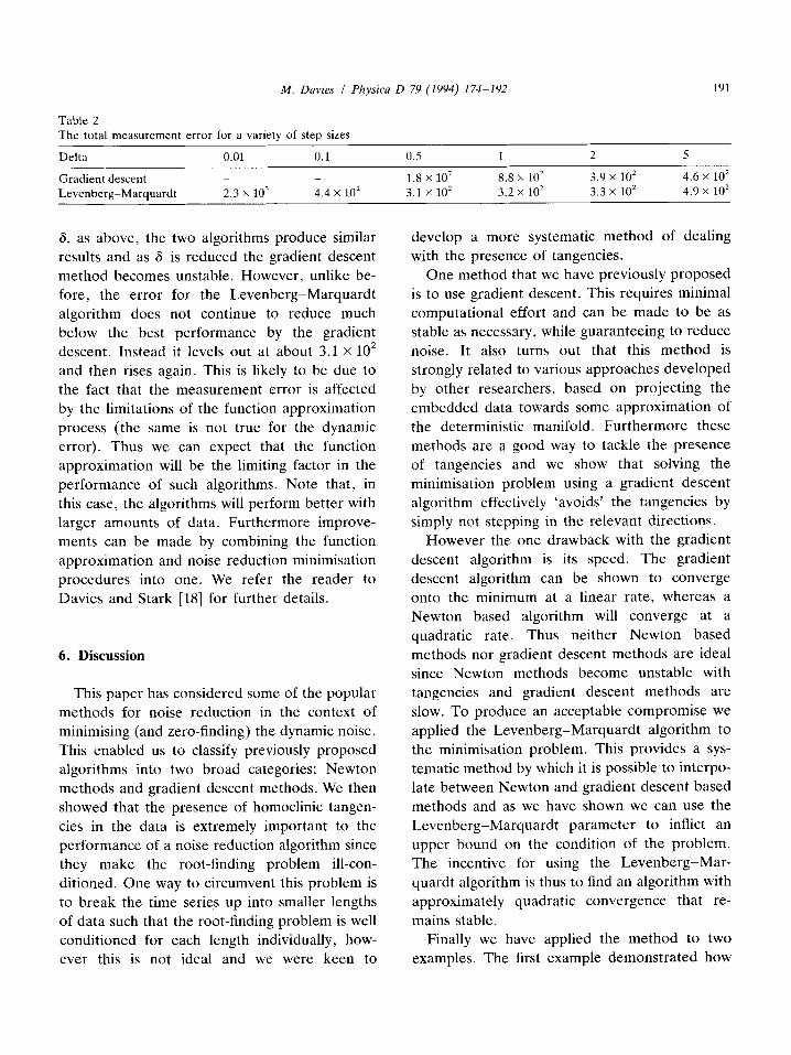
Table 2 The total measurement error for a variety of step sizes

191

Del ta 0.01 0.1 0.5 1 2 5

Gradien t descent - - 1.8 • 107 8.8 x 102 3.9 x 102 4.6 x 102

L e v e n b e r g - M a r q u a r d t 2.3 X 1 0 3 4.4 x 102 3.1 • 102 3.2 • 102 3.3 x 102 4.9 x 102

& as above, the two algorithms produce similar results and as ~ is reduced the gradient descent method becomes unstable. However , unlike before, the error for the Levenberg-Marquardt algorithm does not continue to reduce much below the best performance by the gradient descent. Instead it levels out at about 3.1 x 10 2 and then rises again. This is likely to be due to the fact that the measurement error is affected by the limitations of the function approximation process (the same is not true for the dynamic error). Thus we can expect that the function approximation will be the limiting factor in the performance of such algorithms. Note that, in this case, the algorithms will perform better with larger amounts of data. Fur thermore improve- ments can be made by combining the function approximation and noise reduction minimisation procedures into one. We refer the reader to Davies and Stark [181 for further details.

6. Discussion

This paper has considered some of the popular methods for noise reduction in the context of minimising (and zero-finding) the dynamic noise. This enabled us to classify previously proposed algorithms into two broad categories: Newton methods and gradient descent methods. We then showed that the presence of homoclinic tangencies in the data is extremely important to the performance of a noise reduction algorithm since they make the root-finding problem ill-conditioned. One way to circumvent this problem is to break the time series up into smaller lengths of data such that the root-finding problem is well condit ioned for each length individually, however this is not ideal and we were keen to

develop a more systematic method of dealing with the presence of tangencies.

One method that we have previously proposed is to use gradient descent. This requires minimal computational effort and can be made to be as stable as necessary, while guaranteeing to reduce noise. It also turns out that this method is strongly related to various approaches developed by other researchers, based on projecting the embedded data towards some approximation of the deterministic manifold. Fur thermore these methods are a good way to tackle the presence of tangencies and we show that solving the minimisation problem using a gradient descent algorithm effectively 'avoids' the tangencies by simply not stepping in the relevant directions.

However the one drawback with the gradient descent algorithm is its speed. The gradient descent algorithm can be shown to converge onto the minimum at a linear rate, whereas a Newton based algorithm will converge at a quadratic rate. Thus neither Newton based methods nor gradient descent methods are ideal since Newton methods become unstable with tangencies and gradient descent methods are slow. To produce an acceptable compromise we applied the Levenberg-Marquard t algorithm to the minimisation problem. This provides a systematic method by which it is possible to interpolate between Newton and gradient descent based methods and as we have shown we can use the Levenberg-Marquard t parameter to inflict an upper bound on the condition of the problem. The incentive for using the Levenberg -Mar - quardt algorithm is thus to find an algorithm with approximately quadratic convergence that re- mains stable.

Finally we have applied the method to two examples. The first example demonstra ted how


well the L e v e n b e r g - M a r q u a r d t m e t h o d could

work w h e n the mapp ing func t ion is known. He re

there was very little difference be tween this

m e t h o d and using mani fo ld decompos i t ion . The

second example compared the pe r fo rmance of

the L e v e n b e r g - M a r q u a r d t a lgor i thm to the gra-

d ien t descent me thod . Here the data was t aken

f rom a flow and the dynamics had to be approxi-

ma ted . A l though the L e v e n b e r g - M a r q u a r d t

m e t h o d was no t substant ia l ly be t te r in terms of

an i m p r o v e m e n t in m e a s u r e m e n t er ror it re-

m a i n e d stable for a b roade r range of step sizes

and also pe r fo rmed be t te r in terms of reducing

the dynamic error .

References

[1] E.J. Kostelich and J.A. Yorke, Noise reduction: finding the simplest dynamical system consistent with the data, Physica D 41 (1990) 183-196.

[2] R. Bowen, Markov partitions for Axiom A dif- feomorphisms, Amer. J. Math. 92 (1970) 725-747.

[3] J.D. Farmer and J.J. Sidorowich, Optimal shadowing and noise reduction, Physica D 47 (1991) 373-392.

[4] S.M. Hammel, A noise reduction method for chaotic systems, Phys. Lett. A 148 (1990) 421-428.

[5] T. Schreiber and P. Grassberger, A simple noise reduction method for real data, Phys. Len A. 160 (1991) 411-418.

[6] R. Cawley and G.-H. Hsu, SNR performance of a noise reduction algorithm applied to coarsely sampled chaotic data, Phys. Lett. A 166 (1992) 18-196.

[7] T. Sauer, A noise reduction method for signals from nonlinear systems, Physica D 58 (1992) 193-202.

[8] M. Davies, Noise reduction by Gradient Descent, Int. J. Bifurc. Chaos 3 (1992) 113-118.

[9] P. Grassberger, R. Hegger, H. Kantz, C. Schaffrath and T. Schreiber, On noise reduction methods for chaotic data (1992), preprint.

[10] R. Fletcher, Practical Methods of Optimisation (Wiley, New York, 1980).

[11] F. Takens, Detecting strange attractors in fluid turbulence, Dynamical Systems and Turbulence, Lecture Notes in Math. 898, ed. D. Rand and L-S. Young (Springer, Berlin, 1981).

[12] D.S. Broomhead and G.P. King, Extracting qualitative dynamics from experimental data, Physica D 20 (1987) 217-236.

[13] T. Sauer, J.A. Yorke and M. Casdagli, Embedology, J. Star. Phys. 65 (1991) 579-616.

[14] D.S. Broomhead, J.P. Huke and M.R. Muldoon, Linear filters and nonlinear systems, J. Stat. Phys. 65 (1992).

[15] M. Casdagli, S. Eubank, J.D. Farmer and J. Gibson, State space reconstruction in the presence of noise, Physica D 51 (1991) 52-98.

[16] J.D. Farmer and J.J. Sidorowich, Predicting chaotic time series, Phys. Rev. Lett. 59(8) (1987) 845-848.

[17] D.S. Broomhead and D. Lowe, Multivariate functional interpolation and adaptive networks, Complex Systems 2 (1988) 321-355.

[18] M.E. Davies and J. Stark, A new technique for estimat- ing the dynamics in the noise reduction problem, in: Nonlinearity and chaos in engineering dynamics, eds. J.M.T. Thompson and S.R. Bishop (Wiley, New York, 1993).

[19] W.H. Press, B.P. Flannery, S.A. Teukolsky and W.T. Vetterling, Numerical Recipes in C (Cambridge Univ. Press, Cambridge, 1988).

[20] S.M. Hammel, J.A. Yorke and C. Grebogi, Numerical orbits of chaotic processes represent true orbits, Bull. Amer. Math. Soc. 19 (1988) 465-469.

[21] G.H. Golub and C.F. Van Loan, Matrix Computations (John Hopkins Univ. Press, Baltimore, 1983).

noise reduction schemes for chaotic time series

Documents