non-gaussian statistical appearance models. … · dans ces cas, une analyse quantitative des...
TRANSCRIPT
HAL Id: tel-00008583https://tel.archives-ouvertes.fr/tel-00008583
Submitted on 26 Feb 2005
HAL is a multi-disciplinary open accessarchive for the deposit and dissemination of sci-entific research documents, whether they are pub-lished or not. The documents may come fromteaching and research institutions in France orabroad, or from public or private research centers.
L’archive ouverte pluridisciplinaire HAL, estdestinée au dépôt et à la diffusion de documentsscientifiques de niveau recherche, publiés ou non,émanant des établissements d’enseignement et derecherche français ou étrangers, des laboratoirespublics ou privés.
Non-Gaussian Statistical Appearance Models.Application to the Creation of a Probabilistic Atlas of
Brain Perfusion in Medical ImagingTorbjorn Vik
To cite this version:Torbjorn Vik. Non-Gaussian Statistical Appearance Models. Application to the Creation of a Proba-bilistic Atlas of Brain Perfusion in Medical Imaging. Human-Computer Interaction [cs.HC]. UniversitéLouis Pasteur - Strasbourg I, 2004. English. <tel-00008583>

No d’ordre: 4616THESE
presentee pour obtenir le grade deDocteur de l’Universite Louis Pasteur - Strasbourg I
Ecole doctorale : Sciences pour l’ingenieur
Discipline : Electronique, electrotechnique, automatiqueSpecialite : Traitement d’images et vision par ordinateur
Modeles statistiques d’apparence non gaussiens.Application a la creation d’un atlas probabiliste de
perfusion cerebrale en imagerie medicale
English title: “Non-Gaussian Statistical Appearance Models.
Application to the Creation of a Probabilistic Atlas of Brain Perfusion in Medical Imaging.”
Soutenue publiquementle 21 septembre 2004
par
Torbjørn VIK
Membres du jury:
Mme. Isabelle BLOCH Rapporteur externeM. Jack-Gerard POSTAIRE Rapporteur externeM. Ernest HIRSCH Rapporteur interneM. Philippe RYVLIN Examinateur
M. Fabrice HEITZ Directeur de theseM. Jean-Paul ARMSPACH Directeur de these


Thanks
Working and writing this thesis during four years has been an incredible experience to me. Ithas given me the opportunity to learn a great many things, as well on the professional level ason the personal level. It has further given me the opportunity to work with many competentand resourceful persons. As with most research I believe, the achievement of this thesis hasfollowed a route of ups and downs on which I have not been alone. The interaction with andthe help from my collegues, friends and family has been indispensable and I would hereby liketo express my gratefulness to everybody.
First of all, I would like to thank Isabelle Bloch, Jack-Gerard Postaire and Ernest Hirschfor their careful evaluation and judicious comments concerning the manuscript of this work.I would also like to thank Ernest Hirsch for his guidance as a pedagogical mentor and for hisengagement in organizing bilingual scientific seminars which has permitted me to enlarge myprofessional vision. I would further like to thank Philippe Ryvlin for the interest he has shownin my work, an extremely difficult task for a non-specialist.
I am very grateful for having had the opportunity to work under the guidance of FabriceHeitz and Jean-Paul Armspach who, through engagement and dedication, have created a richand dynamic working environment for me and others. Furthermore, I would like to thankboth for their support and the many discussions we have had during these years.
I thank Daniel Grucker and Jean-Francois Dufourd for having received me at their respec-tive laboratories. A special thank to the personnel and co-workers at both laboratories.
I would also like to thank the persons I have met during my teaching duties, Sophie Kohler,Yoshi Takakura, Jean Martz, Laurent Thoraval and others.
I would like to thank my fellow doctoral students, Marcel Bosc, Sylvain Faisan, VincentNoblet, Rozenn Dahyot, Farid Flitti, Aicha Far and others. In particular, I would like to thankMarcel Bosc, who taught me linux/unix and who took me to a new level of C++ programming.His concern and engagement for out-of-work issues has further been an immense personalenrichement to me. I would also like to thank Sylvain Faison who I could easily win forscientific discussions (mostly futile) through which I again caught pleasure in my work after arude first year. I hope we shall have time again for our scientific and non-scientific bike-rideswhen stuff has calmed down after the thesis. During these years, I have also enjoyed thecompanionship of a long list of internships and temporary workers, most lately Thomas Berst,Nicolas Wiest-Daessle and Samuel Sinapin.
A warm thanks goes to my wife Aude and to my son Emil. You make me a very happyperson. I would also like to thank our families and friends for their support and for manypleasant occasions during these years and in the years to come.

iv

Abstract
Single Photon Emission Computer Tomography (SPECT) is a 3D functional imaging tech-nique that yields information about the blood flow in the brain (also called brain perfusion).This imaging technique has found application in the diagnostics of head trauma, dementia,epilepsy and other brain pathologies. To this end, SPECT images are analyzed in order to findabnormal blood flow patterns. For localized abnormalities such as stroke, this characterizationremains an accessible task, whereas for diffuse and variable abnormalities such as beginningdementia, near-drowning episodes and toxic substance exposure, characterization is difficult.It is therefore necessary to develop quantitative methods in which computer-aided statisticalanalysis can take advantage of information present in a database of normal subjects.
This work deals with the construction and evaluation of a probabilistic atlas of brainperfusion in normal subjects as observed in SPECT images. The goals of such an atlas aretwofold: (1) to describe perfusion patterns of the population represented by the atlas in acompact manner, and (2) to identify statistically significant differences between an individualbrain perfusion pattern and the probabilistic atlas. The successful creation of a computerized,probabilistic atlas may have far-reaching impact on clinical applications where qualitative(visual) analysis of SPECT images is current practice.
Three issues have been central in this work: the statistical models that actually describebrain perfusion, the image processing tools used to make brains “comparable” and the experi-mental evaluation of the atlas. For the first issue, we have explored so-called appearance-basedapproaches. These have been developed in computer vision where they have also been widelyadopted. Recent developments have given these models a proper statistical basis. In thiswork, we have introduced an original non-linear model based on principal component analysis(PCA) and Bayesian estimation theory.
The second issue is related to the spatial normalization of images (i.e. image registration)and intensity normalization. In order to compare brain images coming from different subjects,their relative positions must be found. This is done by calculating a non-linear mapping be-tween corresponding anatomical regions. A registration scheme specifically adapted to SPECTimages had to be developed for this task. Furthermore, since the gray values in SPECT im-ages only represent relative measures of blood flow, the observed values must be normalized toallow for comparison between images. For this we devised an efficient, joint distribution-basedintensity normalization scheme.
Finally, because of the lack of absolute knowledge about the brain perfusion in a normalpopulation, an elaborate evaluation scheme had to be developed. The scheme is based on thedetection of simulated abnormalities combined with a leave-one-out strategy. This scheme wasused to evaluate and compare the different models and normalization schemes considered inthis work. For evaluation on a clinical application, the atlas was also applied to characterizeseizure foci in patients with epilepsy.

Resume en francais
La tomoscintigraphie par emission mono-photonique (TEMP) est une methode d’imageriefonctionnelle 3D qui apporte des informations sur le debit sanguin cerebral (egalement appeleperfusion cerebrale). Cette methode d’imagerie, par la detection visuelle d’anomalies de per-fusion caracterisees par des zones hypo- ou hyper-intenses, est utilisee pour le diagnostic chezdes patients atteints d’accidents vasculaires cerebraux, de demence, d’epilepsie ou d’autres pa-thologies cerebrales. La detection d’anomalies focalisees observees chez les patients ayant uneattaque cerebrale est relativement aisee, alors que les anomalies diffuses, observees en debutde demence, lors d’un accident entraınant une oxygenation insuffisante du cerveau ou suite aune exposition a une substance toxique, sont plus difficilement observables. Dans ces cas, uneanalyse quantitative des images, utilisant un atlas et des outils statistiques s’appuyant sur unebase d’images de cas normaux, peut apporter une aide precieuse au diagnostic.
Le travail presente dans cette these est centre sur la problematique de la construction etde l’evaluation d’un atlas probabiliste de perfusion cerebrale a partir des images TEMP desujets dits normaux. Les objectifs d’un tel atlas sont doubles : (1) creation d’une cartographiestatistique de la perfusion cerebrale d’une population normale, decrite de maniere compacte, et(2) identification des differences de perfusion cerebrale qui sont statistiquement significativesentre une image TEMP d’un individu et l’atlas probabiliste. L’utilisation d’un atlas devraitavoir un impact important sur les applications cliniques ou l’analyse qualitative d’imagesTEMP est pratique courante.
Afin d’atteindre ces objectifs, trois points ont ete abordes : le developpement de modelesstatistiques qui decrivent de facon fidele la perfusion cerebrale, les outils de traitement d’imagesutilises pour rendre les cerveaux « comparables », et enfin, l’evaluation experimentale del’atlas.
Pour le premier point, nous avons explore les approches dites « par modeles d’apparence ».Ceux-ci ont ete developpes dans le domaine de la vision par ordinateur ou ils ont ete largementappliques. Des developpements recents ont redefini ces modeles dans un cadre statistique.Dans ce travail, nous avons introduit un modele original non lineaire et non-gaussien, base surl’analyse en composantes principales (ACP) et la theorie de l’estimation bayesienne.
Le second point est lie a la fois a la normalisation spatiale de l’image (ou recalage d’images)et a la normalisation d’intensite des images. La creation d’un atlas impose de mettre en corres-pondance les differentes structures anatomiques (qui doivent occuper le meme emplacementdans l’espace). Ceci est realise a l’aide d’un recalage non-rigide, c.a.d. une transformation spa-tiale non lineaire. Une methode de recalage specifiquement adaptee aux images TEMP a duetre developpee a cet effet. De plus, puisque les niveaux de gris dans les images TEMP repre-sentent des mesures relatives a la perfusion, les valeurs observees doivent etre normalisees afinde permettre une comparaison entre images. Pour cela, nous avons developpe une techniquede normalisation d’intensite basee sur l’histogramme conjoint des images 3D.
Le dernier point concerne l’evaluation de l’ensemble de la chaıne de traitement. L’absenced’une verite terrain relative a la perfusion cerebrale d’une population ou d’un individu, nousa amene a developper une procedure evoluee d’evaluation. Cette procedure est basee sur ladetection d’anomalies simulees, combinee avec une strategie de validation croisee. La procedurea ete utilisee pour evaluer et comparer les differents modeles et techniques de normalisationdeveloppes dans ce travail. Les performances de notre modele ont ete evaluees dans un cadreclinique pour caracteriser les foyers epileptogenes chez des patients epileptiques.
Le memoire de these est divise en trois parties. La premiere partie decrit le contexte etl’objectif principal des travaux realises. Une introduction a l’imagerie TEMP, au traceur ECD

vii
et aux applications cliniques permet d’apprehender les possibilites et les limites de ce typed’imagerie. Cette introduction permet de situer les difficultes rencontrees, en particulier pourle recalage et la normalisation d’intensite.
La seconde partie est consacree aux developpements theoriques de ce travail, bases surles modeles d’apparence probabilistes. Dans le premier chapitre, nous presentons un etat del’art de ces approches, leurs extensions et leurs variantes ainsi qu’un rappel des techniquesd’estimation statistique robuste (en particulier la theorie semi-quadratique) et des methodesd’estimation de densite non-parametrique (en particulier « Mean Shift »). Avec le mot ap-parence, nous entendons une image representative (une mesure globale) d’un objet. L’idee debase est de representer statistiquement les proprietes caracteristiques d’un objet directementa partir de plusieurs apparences de l’objet, en utilisant des techniques de reduction de di-mension. Les modeles classiques utilisent par exemple l’analyse en composantes principales(ACP). Cependant, de recents developpements ont etendu cette idee originale pour construireun modele statistique complet, connu sous le nom de « ACP probabiliste » (ACPP). L’ACPPest basee sur le modele d’analyse factorielle, qui est un modele a variable latente. Ainsi, lesproblemes classiques en vision par ordinateur, comme la detection ou la reconnaissance desformes peuvent etre reformules dans un cadre d’estimation probabiliste qui se base sur desprincipes tels que : le maximum de vraisemblance (MV) ou le maximum a posteriori (MAP).Dans notre cas, pour l’image consideree, une projection dans un espace reduit (l’espace propre)doit etre estimee.
Dans le chapitre suivant, nous presentons notre modele original. A l’origine, le modeleACPP a ete developpe pour un bruit d’observation de type gaussien. Il existe maintenantdes generalisations a des bruits non-gaussiens, rendant le modele plus robuste. Nous contri-buons a ces extensions en developpant un algorithme qui estime la projection dans l’espacepropre en utilisant le paradigme MAP, avec une distribution a priori dans l’espace propre non-parametrique (estimee par la methode des noyaux) et un bruit non-gaussien. L’algorithme aete developpe en combinant des elements de la procedure non-parametrique « Mean Shift », etde la theorie semi-quadratique [220]. Dans le dernier chapitre, nous concluons cette deuxiemepartie avec des exemples illustrant les performances en classification et detection de ce nouveaumodele sur des images en deux dimensions. L’importance de la modelisation de la distributiona priori y est clairement etablie.
La troisieme partie concerne la construction et l’evaluation d’un atlas de perfusion cere-brale en utilisant le cadre de modelisation statistique decrit ci-dessus. Nous presentons toutd’abord une vue d’ensemble des principales etapes du traitement : modelisation statistique,recalage d’image et normalisation d’intensite. Il existe peu de publications sur l’utilisation d’at-las probabilistes en medecine nucleaire. Nous presentons celles qui existent ainsi que d’autresmethodes apparentees, qui partagent des interets similaires aux notres.
Ensuite nous procedons a une description detaillee de notre approche. Une vue d’ensembledu processus de recalage et des variantes possibles est presentee. Nous detaillons egalement lerecalage non lineaire d’images d’un sujet TEMP en utilisant l’image par resonance magnetique(IRM) du sujet. Les principaux aspects des differents algorithmes utilises pour le recalageTEMP-IRM intra-sujet et le recalage IRM-IRM inter-sujets sont decrits. La suite du chapitredecrit la methode utilisee pour la normalisation de l’intensite. Celle-ci est realisee grace aune regression lineaire sur l’histogramme conjoint en utilisant la methode TLS (« total leastsquares »). A la fin du chapitre, nous resumons les modeles statistiques utilises pour la creationde l’atlas proprement dit. Ces modeles correspondent aux modeles d’apparence presentes dansla deuxieme partie.

viii
Le chapitre suivant decrit l’evaluation de l’atlas. Apres une discussion sur les aspects ge-neraux de la validation dans le traitement d’images medicales, nous examinons les autrestravaux realises sur la validation d’images TEMP quantitatives. Ensuite, nous detaillons leprocede d’evaluation que nous proposons : validation croisee, images de syntheses et criteresd’evaluation (caracteristiques operationnelles de recepteur - COR). Le critere le plus appropriepour la validation d’un modele d’atlas serait un test d’adequation (de type « goodness-of-fit »).Neanmoins, ce critere est inadapte dans notre cas etant donne la grande dimension des images3D (d > 25 000 voxels), une population reduite (N=34 images de test) et l’incertitude de laverite terrain. Notre solution a ete d’utiliser une approche de validation croisee « leave-one-out », combinee avec des modeles de perfusion cerebrale anormale, simulee a partir d’imagesTEMP reelles. Les images resultantes sont analysees afin d’obtenir des courbes COR. Ce cri-tere compose mesure a la fois la capacite du modele a representer les donnees et a detecter desanomalies. Plusieurs resultats importants ont ete obtenus grace a cette etude : un processus derecalage optimal, le nombre optimal de composantes principales a utiliser dans le modele d’ap-parence. La superiorite du modele statistique propose par rapport au modele gaussien ponctuelclassique et l’interet de la generalisation a un bruit non-gaussien en presence d’anomalies detaille importante ont ete etablis. Enfin la sensibilite de la detection a la localisation relativedes anomalies [219, 221] a ete constatee et quantifiee. Nous concluons la troisieme partie enpresentant des resultats obtenus en comparant les images critiques (pendant les crises d’epi-lepsie) et inter-critiques (entre les crises) avec un atlas de sujets normaux dans une applicationclinique concernant la detection des foyers epileptogenes chez des patients epileptiques.
En dehors des developpements theoriques sur les modeles statistiques, une partie impor-tante de ce travail a concerne le developpement logiciel. J’ai contribue de maniere significativeau developpement d’un logiciel libre de traitement d’images en C++, ImLib3D, qui est dis-ponible gratuitement pour les autres chercheurs dans ce domaine [19]. Une autre librairie,gslwrap, qui facilite les calculs d’algebre lineaire en C++ a egalement ete developpee dansun cadre collaboratif de logiciel libre. L’atlas probabiliste a ete implemente en tant que mo-dule dans la plate-forme logicielle Medimax de l’IPB (Institut de Physique Biologique) et duLSIIT (Laboratoire des Sciences de l’Image de l’Informatique et de la Teledetection). Cetteplate-forme est accessible aux medecins et chercheurs de ces deux equipes de recherche.

Contents
I Introduction 1
1 Introduction and overview 31.1 Research environment . . . . . . . . . . . . . . . . . . . . . . . . . . . . . . . 31.2 Approach and general overview . . . . . . . . . . . . . . . . . . . . . . . . . . 41.3 List of contributions . . . . . . . . . . . . . . . . . . . . . . . . . . . . . . . . 61.4 Organization of this document . . . . . . . . . . . . . . . . . . . . . . . . . . . 6
2 Introduction to medical imaging and single photon emission computer to-mography imaging 92.1 Medical imaging and imaging the brain . . . . . . . . . . . . . . . . . . . . . . 92.2 Volumetric brain imaging . . . . . . . . . . . . . . . . . . . . . . . . . . . . . . 102.3 Anatomical and functional brain imaging . . . . . . . . . . . . . . . . . . . . . 102.4 Brain function . . . . . . . . . . . . . . . . . . . . . . . . . . . . . . . . . . . . 132.5 Overview of functional brain imaging techniques . . . . . . . . . . . . . . . . . 132.6 Description of the SPECT imaging procedure . . . . . . . . . . . . . . . . . . 15
2.6.1 Overview, the procedure . . . . . . . . . . . . . . . . . . . . . . . . . . 152.6.2 Injection: biodistribution and physical properties of the
Tc-99m ECD radiotracer . . . . . . . . . . . . . . . . . . . . . . . . . . 162.6.3 Image acquisition . . . . . . . . . . . . . . . . . . . . . . . . . . . . . . 182.6.4 Image reconstruction . . . . . . . . . . . . . . . . . . . . . . . . . . . . 212.6.5 Image interpretation . . . . . . . . . . . . . . . . . . . . . . . . . . . . 21
2.7 Radiation burden . . . . . . . . . . . . . . . . . . . . . . . . . . . . . . . . . . 212.8 SPECT atlases for educational purposes . . . . . . . . . . . . . . . . . . . . . 222.9 Clinical applications . . . . . . . . . . . . . . . . . . . . . . . . . . . . . . . . 222.10 SPECT studies for brain research . . . . . . . . . . . . . . . . . . . . . . . . . 222.11 Conclusion . . . . . . . . . . . . . . . . . . . . . . . . . . . . . . . . . . . . . . 25
II Appearance-Based, Probabilistic Image Modeling 27
3 State of the art 293.1 Introduction, overview . . . . . . . . . . . . . . . . . . . . . . . . . . . . . . . 293.2 General background . . . . . . . . . . . . . . . . . . . . . . . . . . . . . . . . . 30
3.2.1 Appearance . . . . . . . . . . . . . . . . . . . . . . . . . . . . . . . . . 303.2.2 Representing appearance . . . . . . . . . . . . . . . . . . . . . . . . . . 303.2.3 Structure in data . . . . . . . . . . . . . . . . . . . . . . . . . . . . . . 313.2.4 Modeling for classification and detection . . . . . . . . . . . . . . . . . 323.2.5 Probabilistic modeling . . . . . . . . . . . . . . . . . . . . . . . . . . . 33

x CONTENTS
3.2.6 Probability density estimation . . . . . . . . . . . . . . . . . . . . . . . 34
3.2.7 Partial conclusion . . . . . . . . . . . . . . . . . . . . . . . . . . . . . . 34
3.3 The Era of eigenfaces . . . . . . . . . . . . . . . . . . . . . . . . . . . . . . . . 34
3.3.1 Principal component analysis (PCA) . . . . . . . . . . . . . . . . . . . 34
3.3.2 Face recognition with PCA . . . . . . . . . . . . . . . . . . . . . . . . . 36
3.3.3 Non-linear subspace modeling . . . . . . . . . . . . . . . . . . . . . . . 37
3.3.4 Probabilistic modeling with PCA . . . . . . . . . . . . . . . . . . . . . 38
3.3.5 Probabilistic Principal Component Analysis (PPCA) . . . . . . . . . . 39
3.3.6 Analytical PCA . . . . . . . . . . . . . . . . . . . . . . . . . . . . . . . 42
3.3.7 Partial conclusion . . . . . . . . . . . . . . . . . . . . . . . . . . . . . . 42
3.4 Other dimension reduction techniques . . . . . . . . . . . . . . . . . . . . . . . 43
3.4.1 Problem statement . . . . . . . . . . . . . . . . . . . . . . . . . . . . . 43
3.4.2 The intrinsic dimension of a sample . . . . . . . . . . . . . . . . . . . . 43
3.4.3 Classification of techniques . . . . . . . . . . . . . . . . . . . . . . . . . 44
3.4.4 Linear methods . . . . . . . . . . . . . . . . . . . . . . . . . . . . . . . 44
3.4.5 Non-linear methods . . . . . . . . . . . . . . . . . . . . . . . . . . . . . 48
3.4.6 Partial conclusion . . . . . . . . . . . . . . . . . . . . . . . . . . . . . . 50
3.5 Robust estimation . . . . . . . . . . . . . . . . . . . . . . . . . . . . . . . . . 51
3.5.1 Least-squares regression . . . . . . . . . . . . . . . . . . . . . . . . . . 51
3.5.2 M-estimators . . . . . . . . . . . . . . . . . . . . . . . . . . . . . . . . 51
3.5.3 Optimization with half-quadratic theory . . . . . . . . . . . . . . . . . 53
3.5.4 Robust methods with PCA . . . . . . . . . . . . . . . . . . . . . . . . 54
3.5.5 Evaluation of robust techniques . . . . . . . . . . . . . . . . . . . . . . 55
3.6 Non-parametric density estimation and the Mean Shift . . . . . . . . . . . . . 55
3.7 Conclusion . . . . . . . . . . . . . . . . . . . . . . . . . . . . . . . . . . . . . . 56
4 An original non-Gaussian probabilistic appearance model 59
4.1 The basis: global linear model with additive noise (case 1) . . . . . . . . . . . 60
4.1.1 Image reconstruction under the model . . . . . . . . . . . . . . . . . . 61
4.1.2 Model estimation . . . . . . . . . . . . . . . . . . . . . . . . . . . . . . 62
4.2 Generalizing the hypotheses . . . . . . . . . . . . . . . . . . . . . . . . . . . . 63
4.3 Case 2: non-Gaussian noise, uniform subspace distribution . . . . . . . . . . . 64
4.3.1 ARTUR . . . . . . . . . . . . . . . . . . . . . . . . . . . . . . . . . . . 64
4.3.2 LEGEND . . . . . . . . . . . . . . . . . . . . . . . . . . . . . . . . . . 65
4.3.3 Probabilistic interpretation . . . . . . . . . . . . . . . . . . . . . . . . . 65
4.3.4 Interpretation of weights . . . . . . . . . . . . . . . . . . . . . . . . . . 65
4.3.5 Computational issues . . . . . . . . . . . . . . . . . . . . . . . . . . . . 66
4.4 Case 3: non-Gaussian noise, Gaussian subspace distribution . . . . . . . . . . 66
4.5 Case 4: Gaussian noise, non-Gaussian subspace distribution . . . . . . . . . . 67
4.5.1 Non-Gaussian subspace distribution . . . . . . . . . . . . . . . . . . . . 67
4.5.2 Densities under Gaussian noise . . . . . . . . . . . . . . . . . . . . . . 67
4.5.3 Modified Mean Shift . . . . . . . . . . . . . . . . . . . . . . . . . . . . 69
4.6 Case 5: non-Gaussian noise, non-Gaussian subspace distribution . . . . . . . . 69
4.7 Summary of models and algorithms . . . . . . . . . . . . . . . . . . . . . . . . 70
4.8 Conclusion and future work . . . . . . . . . . . . . . . . . . . . . . . . . . . . 70

CONTENTS xi
5 Experiments 75
5.1 Image database description . . . . . . . . . . . . . . . . . . . . . . . . . . . . . 75
5.2 Pose estimation scenario . . . . . . . . . . . . . . . . . . . . . . . . . . . . . . 765.3 Experimental results . . . . . . . . . . . . . . . . . . . . . . . . . . . . . . . . 77
5.4 Discussion . . . . . . . . . . . . . . . . . . . . . . . . . . . . . . . . . . . . . . 82
5.4.1 Overall performance . . . . . . . . . . . . . . . . . . . . . . . . . . . . 835.4.2 Modeling issues . . . . . . . . . . . . . . . . . . . . . . . . . . . . . . . 84
5.4.3 Experimental issues and practical concerns . . . . . . . . . . . . . . . . 85
5.5 Conclusion . . . . . . . . . . . . . . . . . . . . . . . . . . . . . . . . . . . . . . 87
III Brain Perfusion Atlas: Construction and Evaluation 89
6 Models and preprocessing: overview and state of the art 916.1 Atlas, definition . . . . . . . . . . . . . . . . . . . . . . . . . . . . . . . . . . . 91
6.2 Overview, construction and modeling . . . . . . . . . . . . . . . . . . . . . . . 92
6.2.1 Non-probabilistic approaches . . . . . . . . . . . . . . . . . . . . . . . . 926.2.2 Pattern recognition and hypothesis-testing . . . . . . . . . . . . . . . . 94
6.2.3 Experimental design . . . . . . . . . . . . . . . . . . . . . . . . . . . . 946.3 Related work and statistical models . . . . . . . . . . . . . . . . . . . . . . . . 95
6.3.1 Other reviews . . . . . . . . . . . . . . . . . . . . . . . . . . . . . . . . 96
6.3.2 Univariate methods . . . . . . . . . . . . . . . . . . . . . . . . . . . . . 966.3.3 Multivariate methods . . . . . . . . . . . . . . . . . . . . . . . . . . . . 100
6.3.4 Image databases . . . . . . . . . . . . . . . . . . . . . . . . . . . . . . 105
6.3.5 Partial conclusion . . . . . . . . . . . . . . . . . . . . . . . . . . . . . . 1056.4 Registration . . . . . . . . . . . . . . . . . . . . . . . . . . . . . . . . . . . . . 105
6.4.1 Overview . . . . . . . . . . . . . . . . . . . . . . . . . . . . . . . . . . 107
6.4.2 Intra-subject, SPECT-MRI rigid registration . . . . . . . . . . . . . . . 1076.4.3 Inter-subject, MRI deformable registration . . . . . . . . . . . . . . . . 108
6.4.4 Methods for inter-subject SPECT registration . . . . . . . . . . . . . . 110
6.4.5 Integrating registration into the statistical model: modeling anatomicalvariance . . . . . . . . . . . . . . . . . . . . . . . . . . . . . . . . . . . 112
6.4.6 Structural approaches to inter-subject comparison . . . . . . . . . . . . 1126.5 Brain segmentation . . . . . . . . . . . . . . . . . . . . . . . . . . . . . . . . . 113
6.6 Intensity normalization of SPECT images: Existing approaches . . . . . . . . 1136.6.1 A controversial topic . . . . . . . . . . . . . . . . . . . . . . . . . . . . 114
6.6.2 Which transfer function? . . . . . . . . . . . . . . . . . . . . . . . . . . 114
6.6.3 Estimating the transfer function . . . . . . . . . . . . . . . . . . . . . . 1156.6.4 Integrating normalization in the statistical model: ANCOVA . . . . . . 116
6.7 Conclusion . . . . . . . . . . . . . . . . . . . . . . . . . . . . . . . . . . . . . . 116
7 Atlas creation, our approach 119
7.1 Database of normal subjects . . . . . . . . . . . . . . . . . . . . . . . . . . . . 1197.2 Database of patients . . . . . . . . . . . . . . . . . . . . . . . . . . . . . . . . 119
7.3 Spatial normalization: registration . . . . . . . . . . . . . . . . . . . . . . . . . 120
7.3.1 Choice of reference image and reference space . . . . . . . . . . . . . . 1217.3.2 Registration scheme . . . . . . . . . . . . . . . . . . . . . . . . . . . . 122

xii CONTENTS
7.3.3 Application of transformations to SPECT images: combination anddownsampling of deformation fields . . . . . . . . . . . . . . . . . . . . 122
7.4 SPECT brain segmentation . . . . . . . . . . . . . . . . . . . . . . . . . . . . 1257.5 Intensity normalization by total least squares . . . . . . . . . . . . . . . . . . . 1267.6 Statistical models considered . . . . . . . . . . . . . . . . . . . . . . . . . . . . 126
7.6.1 Comparing an image with the atlas . . . . . . . . . . . . . . . . . . . . 1287.7 Atlas creation: estimation of model parameters . . . . . . . . . . . . . . . . . 1287.8 Conclusion . . . . . . . . . . . . . . . . . . . . . . . . . . . . . . . . . . . . . . 130
8 Atlas evaluation 1358.1 The need for validation . . . . . . . . . . . . . . . . . . . . . . . . . . . . . . . 1358.2 The difficulty of validation . . . . . . . . . . . . . . . . . . . . . . . . . . . . . 136
8.2.1 Validating model hypotheses . . . . . . . . . . . . . . . . . . . . . . . . 1368.2.2 Evaluating the model and the influence of preprocessing algorithms . . 137
8.3 Evaluation studies based on simulations . . . . . . . . . . . . . . . . . . . . . . 1398.4 Evaluation in the absence of a ground truth . . . . . . . . . . . . . . . . . . . 1398.5 Proposed evaluation scheme . . . . . . . . . . . . . . . . . . . . . . . . . . . . 1408.6 Results and discussion . . . . . . . . . . . . . . . . . . . . . . . . . . . . . . . 143
8.6.1 Comparing models . . . . . . . . . . . . . . . . . . . . . . . . . . . . . 1438.6.2 Comparing registration schemes . . . . . . . . . . . . . . . . . . . . . . 1468.6.3 Comparing methods for intensity normalization . . . . . . . . . . . . . 1478.6.4 Overall improvement . . . . . . . . . . . . . . . . . . . . . . . . . . . . 1488.6.5 Dependence on location . . . . . . . . . . . . . . . . . . . . . . . . . . 1488.6.6 Comparing validation strategies . . . . . . . . . . . . . . . . . . . . . . 150
8.7 Conclusion . . . . . . . . . . . . . . . . . . . . . . . . . . . . . . . . . . . . . . 150
9 Clinical Application: Epilepsy 1539.1 The pathology . . . . . . . . . . . . . . . . . . . . . . . . . . . . . . . . . . . . 1539.2 Medical imaging and epilepsy . . . . . . . . . . . . . . . . . . . . . . . . . . . 154
9.2.1 SPECT in epilepsy . . . . . . . . . . . . . . . . . . . . . . . . . . . . . 1549.3 Computer-aided evaluation and SISCOM . . . . . . . . . . . . . . . . . . . . . 155
9.3.1 Intensity normalization revisited . . . . . . . . . . . . . . . . . . . . . . 1559.3.2 Difficulties with SISCOM . . . . . . . . . . . . . . . . . . . . . . . . . 156
9.4 Added value of an atlas . . . . . . . . . . . . . . . . . . . . . . . . . . . . . . . 1579.4.1 Cost of an atlas . . . . . . . . . . . . . . . . . . . . . . . . . . . . . . . 1589.4.2 Evaluation revisited . . . . . . . . . . . . . . . . . . . . . . . . . . . . . 158
9.5 Results on real images . . . . . . . . . . . . . . . . . . . . . . . . . . . . . . . 1599.5.1 Similarities and dissimilarities between SISCOM and atlas . . . . . . . 1599.5.2 Similarities and dissimilarities between the atlas models . . . . . . . . . 1609.5.3 Affine versus deformable registration . . . . . . . . . . . . . . . . . . . 164
9.6 Conclusion and future work . . . . . . . . . . . . . . . . . . . . . . . . . . . . 164
10 Conclusions and future work 16710.1 Summary and discussion . . . . . . . . . . . . . . . . . . . . . . . . . . . . . . 16710.2 Future work . . . . . . . . . . . . . . . . . . . . . . . . . . . . . . . . . . . . . 169
10.2.1 Model . . . . . . . . . . . . . . . . . . . . . . . . . . . . . . . . . . . . 16910.2.2 Atlas, model . . . . . . . . . . . . . . . . . . . . . . . . . . . . . . . . . 17010.2.3 Atlas, application . . . . . . . . . . . . . . . . . . . . . . . . . . . . . . 171

CONTENTS xiii
IV Appendix 173
A Modified Mean Shift 175A.1 Modified Kernel Estimate . . . . . . . . . . . . . . . . . . . . . . . . . . . . . 175A.2 Simplified Modified Mean Shift . . . . . . . . . . . . . . . . . . . . . . . . . . 177
A.2.1 An alternative way of obtaining the simplified modified mean shift . . . 177A.3 Convergence Proof of the Modified Mean Shift . . . . . . . . . . . . . . . . . . 178
B Small sample size and covariance matrix decomposition 181
C Peer-reviewed publications by the author 183

xiv CONTENTS

Notation
We keep a coherent notation throughout this thesis. Mathematical symbols that occur recur-rently are tabulated below to facilitate reading. As a general rule, matrices and vectors aretypeset in bold, whereas scalars have a normal typeface. We do not make a notational dis-tinction between random variables and their realizations apart from the case of noise/residual(see below). Transposes are denoted by the superscript T .
VectorsSymbol Signification First reference
y = (y1 · · · yD)T images, observations in observation space
Sec. 3.3.1, p. 34
x = (x1 · · ·xQ)T subspace variable, transformed variablewq eigenvector or subspace vectorε random noise variable
e = (e1 . . . eJ)T residual (i.e. realization of ε)t z-score image Sec. 6.3.3, p. 100b robust weights in half-quadratic optimization Sec. 3.5.3, p. 53Θ general parameter vector
γ and β parameters for linear regression and intensitynormalization
Sec. 3.5.1, p. 51
cj constants in modified mean shift Sec. 4.5.2, p. 68
MatricesSymbol Signification First reference
Σ covariance matrix
Sec. 3.3.1, p. 34W = [w1 . . .wQ] matrix of orthogonal vectors (e.g. eigenvec-
tors or scaled eigenvectors)Y mean-free sample matrixA general purpose matrixR rotation matrix Sec. 3.3.5, p. 39IQ Q×Q identity matrix
B = diag(b) robust weights in half-quadratic optimization Sec. 3.5.3, p. 53
FunctionsSymbol Signification First referenceψ(·) half-quadric expansion 1-dimensional
Sec. 3.5.3, p. 53Ψ(·) half-quadric expansion D-dimensionalQ(·) quadratic expansion in half-quadratic theory
IndexesSymbol Signification First reference
i general purposej=1...J index of subjects, samples or images
Sec. 3.3.1, p. 34d=1...D observation space index (voxel index)q=1...Q subspace indexp=1...P patches of local linear models Sec. 3.4.5, p. 48k=1...K mixture components in mixture model,
activation in activation studiesSec. 3.4.5, p. 48

xvi CONTENTS
Abbreviations
Commonly used abbreviations used in thesis are tabulated below.
Abbreviation SignificationIPB Institut Physique Biologique
SPECT Single Photon Emission Computer TomogropaphyMRI or MR Magnetic Resonance Imaging
ECD Ethyl Cysteinate DimerHMPAO Hexamethyl Propylamine OximeFWHM Full Width at Half Maximum
pdf probability density functioni.i.d. identically and independently distributedLS Least SquaresML Maximum Likelihood
MAP Maximum A PosterioriPCA Principal Component analysis
PPCA Probabilistic Principal Component analysisEM-algorithm Expectation-Maximization algorithm
ANOVA Analysis of varianceANCOVA Analysis of covariance
MANCOVA Multivariate analysis of covarianceROC Receiver Operating Characteristicsi.e. that ise.g. for example

Part I
Introduction


Chapter 1
Introduction and overview
Single Photon Emission Computer Tomography (SPECT) is a 3D functional imaging tech-nique that yields information about the blood flow in the brain (also called brain perfusion).This imaging technique has found application in the diagnostics of head trauma, dementia,epilepsy and other brain pathologies. To this end, SPECT images are analyzed in order to findabnormal blood flow patterns. For localized abnormalities such as stroke, this characterizationremains an accessible task, whereas for diffuse and variable abnormalities such as beginningdementia, near-drowning episodes and toxic substance exposure, characterization is difficult.It is therefore necessary to develop quantitative methods in which computer-aided statisticalanalysis can take advantage of information present in a database of normal subjects.
The goal of this work has been the construction and evaluation of a probabilistic atlasof brain perfusion in normal subjects as observed in SPECT images. The purposes of suchan atlas are twofold: (1) to describe perfusion patterns of the population represented by theatlas in a compact manner, and (2) to identify statistically significant differences between anindividual brain perfusion pattern and the probabilistic atlas. The successful creation of acomputerized, probabilistic atlas may have far-reaching impact on clinical applications wherequalitative (visual) analysis of SPECT images is current practice.
1.1 Research environment
This thesis has been pursued in a cooperative setting between the two research groups Models,Images and Vision (MIV) at the Laboratoire des Sciences de l’Image, de l’Informatique et dela Tı¿1
2lı¿1
2tection (LSIIT – UMR 7005 CNRS), and the image processing group at Institut de
Physique Biologique (IPB – UMR 7004 CNRS). Both LSIIT and IPB are joint laboratoriesof the University of Strasbourg and the french national scientific research organization CentreNational de la Recherche Scientifique (CNRS).
MIV is a group that is specialized in image processing and interpretation in general. Itpursues fundamental research in computer vision and cooperates with other laboratories suchas IPB or Laboratoire Rı¿1
2gional des Ponts et Chaussı¿1
2es (i.e. regional roads and bridges
laboratory – LRPC). The image processing group at IPB pursues image processing researchapplied to medical imaging. It bridges the gap between fundamental vision research and itsapplication in medical research and clinical use. IPB is an interdisciplinary institute where notonly physicians and biologists work together, but also psychologists, neurologists and othermedical experts cooperate. In particular, there is a nuclear medicine facility affiliated with theinstitute that provides the nuclear imaging services at the university hospital of Strasbourg.

4 Introduction and overview
The SPECT images that have been studied in this thesis have been acquired at this nuclearmedicine service.
Other works have been achieved in this setting. In particular, we would like to mentionthose of C. Nikou [171], O. Musse [165], and M. Bosc [17], as well as the ongoing works ofV. Noblet (thesis) and S. Sinapin (technology transfer project, Plamaivic). Together with theworks of Hamdan [87] (MIV) and R. Dahyot [46] (cooperation MIV – LRPC), these worksform the precursors and the building elements on which the developments in this thesis arebased.
1.2 Approach and general overview
Fig. 1.1 shows a problem-oriented view that can be used to describe the global approach takenin this thesis. As we shall see in the next chapter, SPECT images are difficult to interpret,even for a trained person. This is because these images are diffuse in appearance and becausethe anatomical variation between subjects is large, whereas the variation in perfusion (imageintensities) at a given region of the brain may be subtle and difficult to describe and quantify.This is the reason why we have attacked the statistical modeling problem with methods forunsupervised learning. The main focus of this work has thus been the development of suchmethods, which are not limited to our particular problem, but also find use in general patternrecognition and image analysis applications.
Problem:Atlas creation
Image-atlas comparison
Evaluation/validationSoftware development
Unsupervised learningStatistical models
Image processing tools"Making brains comparable"
Computer tools,image database
management
Figure 1.1: A problem oriented view of our approach.
Based on earlier work in our team (Dahyot [46], Hamdan [87]), we have been interested ina particular class of global linear models called appearance-based models. However, to preparethe images for statistical modeling, it is necessary to “make brains comparable”, that is, toperform spatial registration and intensity normalization on brain images of different subjects.Image processing tools which makes this possible have been developed in earlier works (Nikou[171], Musse [165]) and ongoing works (Noblet, Sinapin). However, as we experienced, specialadaptations had to be made.
Because of the large number of images and intermediate images resulting from differentimage processing steps, specific tools for managing these had to be developed. Finally, thelast axis that has been central in this work is the systematic evaluation and comparison of the

1.2 Approach and general overview 5
Technical platform/system
- Software libraries- Data management- Image acquisition- Image databases
Applications
Brain perfusiondisorders
- Research- Clinical
Computer vision
- Pattern modeling - Pattern recognition- Image understanding- Change detection
Innovative & Enabling technologies
Validation & Requirements
- Statistical analysis &modeling- Machine learning- Physics- Algorithms- Software engineering
Engineering researchfundamental knowledge
Figure 1.2: A system view of research and application, seen from the point of view of acomputer scientist.
developed methods. Since no absolute knowledge about normal brain perfusion exists, thisissue has been particularly difficult.
The importance of validation and evaluation can also be seen in Fig. 1.2. This figureshows an overview that relates fundamental research, technical platform and applications.This provides an alternative view for situating the analyses, developments and contributionsthat have been achieved during this thesis. In this overview, we see that an application,such as the creation of a brain perfusion atlas, is enabled through theoretical and fundamentalmethods and is realized by means of a technical platform/system. This relationship is the samefor the application of technologies and knowledge to problems in computer vision. The arrowsshow the relationships between groups. For example, the clinical application of a methodnecessitates its validation. The validation again imposes requirements to the method. Themethod in turn requires a validation of the underlying algorithm (e.g. proof of convergence).Imposing such requirements can be very helpful in the development of new algorithms andmethods. It may even give rise to new theoretical ideas. In the other direction we have thattheoretical developments can enable new applications, and the circle is closed.
The basic idea in this work has been to use and eventually extend techniques that havebeen successfully applied in computer vision (appearance-based models) as well as algorithms,which existed as software libraries (registration), to address our application in brain perfusiondisorders.

6 Introduction and overview
1.3 List of contributions
The original contributions of this work are:
• Bibliographical/theoretical:
– An in-depth review of appearance-based models for image modeling. We developthe exact relationship between two popular and similar probabilistic models.
– A novel, non-Gaussian appearance-based model and the associated algorithms. Thismodel can be used for pattern recognition and image modeling in general.
– A review of statistical models used for SPECT/PET brain atlases.
• Methodological:
– A sophisticated registration scheme for inter-subject, SPECT-MRI matching, basedon existing algorithms.
– An intensity normalization technique for SPECT images.
– A comprehensive evaluation study for comparing atlases and image processing tech-niques.
• Applicative:
– The application of a non-Gaussian statistical model to the creation of a brain per-fusion atlas.
– Contributions to an open-source platform for medical image processing developedusing modern software engineering techniques.
A more detailed description of these contributions is given in the conclusion of this manuscript(Ch. 10).
1.4 Organization of this document
The manuscript is divided into three separate parts. In Ch. 2 we present an introductionto SPECT imaging, the ECD radiotracer and their clinical application. This introductionfamiliarizes the reader with this imaging modality, some of its possibilities and limitations.This familiarity helps him to understand some of the later discussions on the difficulties en-countered, particularly the registration and intensity normalization issues.
The second part is devoted to the theoretical developments of this work. These are basedon appearance-based models. In Ch. 3, we present a state of the art of such approaches, theirextensions and variations. We also review techniques for robust estimation (i.e. half-quadratictheory) and non-parametric density estimation/mode detection (i.e. Mean Shift). These ele-ments compose the foundations of our original non-Gaussian model, which is presented in Ch.4. Finding the exact maximum likelihood estimates of the model parameters of this modelis difficult. Furthermore, a prerequisite to this phase of learning is what we call the recon-struction problem. This problem is defined and then solved for a series of increasingly moregeneral models. This solution opens up the perspective of solving the learning problem to

1.4 Organization of this document 7
which currently an approximative solution is used. To assess the model, a comprehensive clas-sification experiment is performed on a standard computer vision database. This experimentis described in Ch. 5.
In part three, we turn our attention to the construction and evaluation of a probabilisticbrain perfusion atlas using the above described statistical modeling framework. In Ch. 6, wefirst present an overview of the main processing steps: statistical modeling, image registrationand intensity normalization. There are only few reports of the use of general-purpose, proba-bilistic atlases in the nuclear medicine literature. We propose a review of these together withsome related methods that share concerns that are similar to ours.
In Ch. 7, we then proceed to a detailed description of our approach. An overview of theregistration scheme and possible variations is presented. We detail the non-linear, inter-subjectregistration of SPECT images by co-registering each subject with its associated MR imageand we describe the total least squares method used for intensity normalization. Finally, thedifferent statistical models on which we have performed our evaluation studies are summarizedat the end of chapter 7. They correspond to the appearance-based models presented in Ch.4, part two.
Ch. 8 describes the atlas evaluation. We first discuss some general aspects of validation inmedical image processing and review other work in quantitative SPECT image validation. Wethen detail our proposed evaluation scheme: leave-one-out, synthesized images and evaluationcriterion (receiver operating characteristics - ROC analysis). The evaluation study was used tocompare different models, registration schemes, intensity normalization and the dependencyof the atlas performance to brain location. We present and discuss the results of these com-parisons at the end of Ch. 8. Part three is concluded by Ch. 9, where we present preliminaryresults obtained by comparing images of patients with epilepsy to the atlas.
The thesis is summarized and concluded in Ch. 10 where we also discuss some possiblepaths for future research.

8 Introduction and overview

Chapter 2
Introduction to medical imaging andsingle photon emission computertomography imaging
The purpose of this chapter is to acquaint the reader with the characteristic properties ofSPECT images. We begin with a brief introduction to medical imaging and, more specifi-cally, techniques for imaging the brain. This allows us to situate SPECT imaging and betterunderstand its particular position among the many techniques that exist. We then give anintroductory description of the procedure of acquiring SPECT images, how the radiotraceris distributed in the body and to the brain, how the emitted gamma-rays are transformedto voltage pulses, and how the transversal slices are reconstructed from projections. We thentouch upon other issues like image interpretation, clinical applications of SPECT imaging withexamples, as well as the important issue of radiation burden.
2.1 Medical imaging and imaging the brain
Medical imaging is an extraordinary example of multidisciplinary research. It originated withradiation physics and with the discovery of X-rays in 1895 by Roentgen. The applicationfor medical purposes was immediate. Today, additional knowledge from medicine (anatomy,histology, physiology, pathology), biology and cytology (tissue, cells and their interaction),chemistry (radiopharmaceuticals) mathematics, signal processing and computer science, aswell as high precision mechanics (rotating cameras) and electronics (computers, superconduc-tors) have led to the development of a multitude of different techniques that are used on aroutine basis. Today medical imaging represents a series of ubiquitous tools for diagnosis,treatment and medical research.
The multitude of techniques does not however mean that there is no need to continueresearch on medical imaging. Many questions still remain open concerning the way the bodyfunctions and how pathologies develop. In particular, the last 15 years have shown manyadvances in brain research and the associated development of brain imaging techniques. Suchdevelopment aims at creating new imaging techniques that make it possible to “see” new oralternative aspects of the brain, improving the resolution of existing techniques, reducing costsof imaging, or reducing patient and personnel inconvenience (time of scan, radiation burden,invasiveness etc.). Furthermore, they bring new insights in physiology, biology and pathology.
In this presentation we do not intend to give a review of all imaging techniques applied in

10 Introduction to SPECT Imaging
Figure 2.1: Progress in medical imaging. On the left: Mrs. Roentgen’s left hand (1895). Onthe right: modern X-rays.
medicine. For this, we refer the reader to [37] for a more technical understanding of the physicalprinciples of MRI, SPECT, PET and ultrasound as well as the mathematical foundations fortomographic reconstruction of images from projections. For an introduction to the applicationand interpretation of such images, course material from radiology is adequate [98].
Imaging the brain helps us to improve our understanding of how the brain works and howpathologies develop. Research in this domain has led to more accurate diagnosis and bettertreatments of brain pathologies. The understanding of how the brain works has fascinated manfor a long time, but it also poses philosophical and ethical questions. Consider for example thecombination of marketing and brain research, “Neuroeconomy”1, where a better understandingof how the brain works will be used to influence the habits of consommation.
2.2 Volumetric brain imaging
Modern medical imaging began with the development of computer tomography in 1972 by G.N. Hounsfield [103]. The reconstruction of slices and volumes from projections obtained fromdifferent angles around the body makes it possible to “see” inside the body. We can observestructures, physiological parameters and their relative positions in space. All images of thebrain in this work are three-dimensional, either from stacking transaxial slices (SPECT) orfrom true reconstructed images in three-dimensions (MRI). See Fig. 2.2 for an explanation ofmultiplanar visualization and notation.
2.3 Anatomical and functional brain imaging
We can distinguish between anatomical and functional techniques for brain imaging. Anatom-ical imaging techniques make images of the brain tissue which mainly yield information as tothe relative position of brain structures and organs. Functional techniques make images ofsome physiological process, and thus yield additional information on how the brain works. Weshall describe functional techniques shortly in Sec. 2.5. Anatomical imaging comprises X-raytomography and MR (magnetic resonance) imaging. By intraveneously injecting a contrast
1Frankfurter Allgemeine Zeitung, 05.11.2003, Nr. 257. See also: http://www.neuroeconomy.org

2.3 Anatomical and functional brain imaging 11
sagittal
axial or transaxial
coronalright left
superior
inferior
anterior
posterior
Figure 2.2: Multiplanar visualization of three-dimensional brain images and some basic no-tation for orientation. The three slices or planes are denoted coronal, sagittal and axial (orsometimes transaxial) slices. A cursor marks the intersection between the three planes (from[17]).
agent, X-ray images can be obtained with enhanced contrast of certain features, for example,arteries. In MR imaging one can adjust a large number of parameters (impulse sequence) toobtain different contrasts between different molecules (water, lipides etc.). Fig. 2.3 shows anexample T2-weighted2 MR image, which are the type of MR images used in this work. The res-olution of these images is 1mm3. This is far from capable of imaging cells and neurons (∼ 0.01mm), but we can distinguish gray and white matter as well as the different macrostructuresof the brain.
Anatomical images such as MRI provide important information in many pathologies suchas multiple sclerosis, cerebrovascular diseases, dementia and cancer. This is particularly truewhen the disease leads to tissue changes (atrophies). However, some pathologies are notassociated with morphological changes, or only at a late stage of the disease. Instead changesin physiological parameters such as regional cerebral blood flow (rCBF) can be symptomaticof a disease. In such cases functional images provide important insight. For example, in orderto decide on the proper medication for patients with early signs of dementia, it is importantto distinguish whether they have Alzheimer’s disease or not. This can be done with SPECT(single photon emission tomography) or PET (positron emission tomography) imaging sincecharacteristic patterns of rCBF in Alzheimer’s disease distinguish the disease from other formsof dementia.
Functional images do contain some morphological or structural information about thebrain, but typically at a much lower resolution than MR images and X-ray (CT) images.Thus, in order to precisely locate abnormal functional lesions, the functional and anatomicalimages are often fused together (superimposition), see Fig. 2.4. This is possible due to moderncomputer algorithms that find the relative locations of corresponding brain structures in twoimages obtained by different imaging techniques.
2T2 signifies a particular parameter setting for acquiring MR images.

12 Introduction to SPECT Imaging
Figure 2.3: Example of a T2-weighted MR image of 1mm3 resolution. Only a magnified partof the image is shown. This is what we call an anatomical image, gray and white matter aswell as different macrostructures of the brain can be identified.
Figure 2.4: Example of an abnormal perfusion patterns (hot color coded) detected usingSPECT. The pattern is superimposed on the T2-weighted MR image of the same patient forprecise localization. A patient with epilepsy.

2.4 Brain function 13
2.4 Brain function
In the literature, the term“brain function” is somewhat loosely applied to mean one or more ofseveral things: (1) cognitive brain function (memory, planning, etc.) or sensomotorical tasks(audiovisual tasks, walking, etc.), (2) neurons and neuronal networks (topological organization,signaling etc.) or (3) biochemical or electrical activity (metabolism, glucose consumption,blood oxygenation level, etc.). When reading brain imaging literature, it is useful to be awareof these different levels of brain functions.
In this work we shall consider a functional image to be a macroscopic (with respect toneurons), spatiotemporal measure of one of the activities associated with the third group.These measures are related to cognitive or sensomotorical functions in different ways. Forexample the regional cerebral brain flow (rCBF) is believed to be linearly related to neuronalactivity around a level of resting state [180, p.11]. The neuronal activity will depend onthe way a cognitive or a sensomotorical task is organized. Here, two models exist: that offunctional segregation (specialization) and that of functional integration [67]. Simplifying, onecould say that the former considers that the execution of a specific task (for example fingertapping) is a result of neuronal activity in a cluster of neurons. The latter considers that aspecific task results from the mediation of remotely located neurons. Which model is actually“correct”, probably depends on the task at hand (e.g. most sensomotorical tasks are of theformer type). There could also be a combination of both. The difference has consequences forthe statistical analysis in so-called activation studies and will be further discussed in Ch. 6.
Higher cognitive tasks are modeled at a higher level of interconnected “areas” (languagearea, audio area, etc.) and their cooperation. The connections between image analysis, statis-tics and neurology leads to the different usages of the expression “brain function”. However,from a medical viewpoint, what is important is that different pathologies can manifest them-selves as abnormal functioning of one or more of these types. Furthermore, such abnormalitiescan either be seen in the images of brain function, in neuropsychological tests of brain function,or (mostly) in a combination of both.
2.5 Overview of functional brain imaging techniques
To situate brain SPECT imaging, we briefly describe the different non-invasive imaging tech-niques used for functional brain imaging. Many techniques are complementary in their clinicalaccessibility and the biochemical characteristics they image. Furthermore, there is a tendencyto trade-off between spatial and temporal resolution with the different techniques. A compar-ison of different functional imaging techniques and their temporal and spatial resolving poweris shown in Fig. 2.5. We can distinguish between ionizing techniques (PET, SPECT), func-tional magnetic resonance imaging (fMRI) and techniques based on measuring electromagneticpotentials (MEG/EEG).
Positron emission tomography (PET) and single photon emission computer tomography(SPECT) are ionizing techniques. Here, the image is created by detecting nuclear radiationwhich is emitted from the brain after injecting a radioactive pharmaceutical. The pharma-ceutical is a molecule that imitates a substance which is implicated in a specific biochemicalprocess, for example glucose or oxygen consummation. The pharmaceutical contains a radionu-clide that emits either positrons (PET) or gamma rays (SPECT). These are then detected witha gamma camera. Examples of radiopharmaceuticals used in brain SPECT is HMPAO (Hex-amethyl Propylamine Oxime) and ECD (Ethyl Cysteinate Dimer), the latter will be described

14 Introduction to SPECT Imaging
Spa
tial r
esol
utio
n (m
m)
10
5
15
20
1 10 100 1000 10 000 100 000
Temporal resolution (ms)
Invasive EEG
MEG
fMRI
SPECT
PET
EEG
Lesions
Invasiveness
Low Medium High
Figure 2.5: Overview of functional imaging techniques of the brain and their spatial andtemporal resolving power (from [93]). The term functional can be interpreted at differentlevels. It can mean a biochemical functioning (often in resting state), or it can mean acognitive function, such as recognizing words or images. Typical lesions shown for reference.
in more detail in 2.6.2. Because of better resolution, sensitivity and homogeneity, PET imagingis considered to be superior to SPECT imaging. There are however distinct applications whereSPECT imaging is more appropriate than PET. In addition, a small cyclotron is necessary tocreate PET images because the radionuclides used in PET are short-lived The instrumenta-tion for PET is thus substantially more complex and more costly and as such limited to a fewimaging centers.
Functional MRI (fMRI) is based on the measurement of the oxygenation level in the bloodsupplying the neurons. Activity in a group of neuronal cells augments the consumption ofoxygen, which leads to changes in the concentration of oxygen carrying haemoglobin in theblood. Since the magnetic properties of the haemoglobin with and without oxygen are different,these changes can be measured using magnetic resonance imaging. Functional MRI is mostwidely used in research in order to map cognitive brain function in the normal and pathologicalbrain. Because of the low signal-to-noise ratio, such studies are done by acquiring a series ofimages where the subject repeats a cognitive task. This time series is then analyzed withstatistical tools. This is a so-called activation study, to which we shall have more to say inSec. 6.2.3.
Magnetoencephalography (MEG) and electroencephalography (EEG) can measure mag-netic induction outside the scalp or electric potentials on the scalp produced by electricalactivity in groups of neural cells. This activity is again a result of the functional level in thebrain. MEG and EEG have very high temporal resolution, but their spatial resolution is lessthan or equal to that for SPECT.
As a new emerging technique, diffuse optical tomography (DOT) [15], might also findapplication in measuring brain blood volume and fast changes therein, however it has lower

2.6 Description of the SPECT imaging procedure 15
Figure 2.6: Photo of the gamera camera (left) used at our institute and the control room(right). The camera has two heads that are controled by a motor (behind). The patientis placed on the bed with an additional support for his head. The camera heads are thenpositioned as close as possible to the patient’s head. During acquisition, the camera headsrotate around the axis of the patient and the patient is asked to remain still. The acquisitionprocedure can be programmed and for brain SPECT, two 180 degrees rotations of the camerasare made with acquisitions (projections) at every 4 degrees for 10 seconds. The total acquisitiontime is about 20 minutes.
spatial resolution than fMRI. For this, DOT has still to be finalized for clinical application.
2.6 Description of the SPECT imaging procedure
2.6.1 Overview, the procedure
In order to better understand what the SPECT images represent, let us describe in some detailhow they are obtained and the physics behind their creation. The brain SPECT procedure fol-lows a standard protocol (similar to the guideline proposed by the Society of Nuclear Medecine[177]) to assure that the image acquisition conditions rest as stable as possible between scans.
A picture of the gamma camera that is installed at the service of nuclear medicine at theinstitute of physics and biology (IPB) is shown in Fig. 2.6, and an overview of the differenttime-steps of the imaging procedure is shown in Fig. 2.7. The injection itself is administeredwhen the subject is seated in a comfortable position in a quiet room, keeping his eyes openand relaxing. After injection, the subject remains seated for five minutes. Image acquisitiononly starts after about 20-30 minutes. The subject lays down on a table with a support forthe head. The double-headed camera is positioned so that the rotating center allows thecameras to be as close as possible to each other without touching the patient. During theacquisition itself, which takes another 20-30 minutes, the subject is asked to move as little aspossible. The whole procedure takes about an hour for the patient. After the projections havebeen acquired, the image is reconstructed by the computer before it can be transfered to the

16 Introduction to SPECT Imaging
t (min)0 5
Tracer injectionand fixation
Period of rest
30
Image acquisition
55 65
Imagereconstruction
Image interpretation and written report by specialist
Patient ~1h
125
Figure 2.7: Timetable (approximate) and overview explaining the SPECT imaging procedure.For the patient, the procedure takes about an hour after the tracer has been injected. It is aprerequisite that the patient is capable of remaining immobile during the time of image acqui-sition (mostly 20 minutes in clinical practice, sometimes 30 minutes for research protocols).
physicians workstation for interpretation.In the following, we will describe these different steps and their physical and physiological
properties.
2.6.2 Injection: biodistribution and physical properties of the
Tc-99m ECD radiotracer
A radiotracer used for medical imaging must have properties that fulfill several criteria. Thesecan be separated into physical, biological and chemical. Physical properties concern aspectsthat touch upon technicalities of the imaging technique such as statistical properties of disin-tegration (half-life) and the wavelength of the emitted photons. These aspects are importantfor practical concerns since a long half-life makes it possible to prepare the radionuclide indedicated centers, and photons are easier to detect at certain wavelengths than others. Thebiological properties concern the distribution of the product in the body and the target organ,how it is cleared out (and the associated burden of radiation for the patient), and finally howthe uptake relates to the physiological function of the organ under study (e.g. whether thereis a linear relationship or not). It is under these constraints that a chemically stable moleculemust be found that can serve as a tracer.
The radiopharmaceutical used at IPB for brain SPECT imaging, Technetium-99m ethylcysteinate dimer (ECD), also called bicisate, is one such molecule. The radionuclide Technetium-99m is the main tracer for clinical imaging, and it was among the first tracers to be clinicallyused. It has a half-life of 6.03h and emits photons of 140 keV that are easily detectable using agamma camera [37]. Technetium-99m is obtained from desintegration of Molybden-99, whichhas a half-life of about 66h. Because of this relatively long half-life time, Molybden is deliv-ered only once a week to the institute. Using another assembly kit (Neurolite r© from DuPontPharma), doses that are ready for injection are prepared on-site. Typically, two differentquantities are used, one for adults and a smaller quantity for children.
The ECD radiotracer (Bicisate) is an indicator of cerebral blood flow. When injected,the tracer is rapidly distributed to the brain [216, 141]. This happens because the bicisateis trapped in the brain cell after metabolism, subsequent to its crossing of the blood brain

2.6 Description of the SPECT imaging procedure 17
Blood vessel
Membrane(blood brain barrier)
Tracer molecules
Passive diffusion
Brain cell
Figure 2.8: The brain vessels are equiped with a selective membrane (filter in technical terms) –called the blood brain barrier – through which only certain molecules can pass (glucose, certainproteins etc.). The molecules react chemically with a transporter molecule, water or fat, thatpasses through the barrier by passive diffusion. When the transporter molecule is a fat (water),the molecule that is transported is said to be a lipophilic (hydrophilic). The TC-99m ECDtracer is a lipophilic. Once the ECD tracer has entered the brain cell it undergoes a biochemicaltransformation (ester hydrolisis) and becomes a charged acid metabolite. This metabolite isunable to exit the brain – it becomes trapped.
barrier (by passive diffusion), see Fig. 2.8. The concentration of the tracer in the blood dropsto less than 10% of the inital dose after only one minute.
Bicisate has the desirable property of washing out very slowly from the brain (biexponentialwith half-lives of 1.3 hr (40%) and 42.3 hr (60%)), contrary to other tissues, from which itis cleared out quickly. In particular, face tissue, neck and scalp is cleared rapidly so that thebrain to crane signal is high. This is why image acquisition only starts about 20-30 minutesafter injection. The product is finally cleared from the body by the renal and the hepatobiliarysystem.
Studies have shown that the uptake of bicisate is proportional to the regional cerebralblood flow (rCBF) [42]. The uptake is normally greater in the cortical grey matter where theblood flow is higher than in the white matter. The ratio of grey matter to white matter uptakeis normally greater than 2:1.
Radioactive disintegration: Poisson noise
The radioactive disintegration is a random process and the detected number of gamma photonswithin a period of time follows a Poisson distribution [90]. The number of photons capturedover a constant period of time follows the equation:
P (k) =µke−µ
k!(2.1)
Here, P (k) is the probability of emitting k photons and µ is the (usually unknown) mean. Thevariance of the Poisson distribution, σ2, is equal to the mean µ and implies that the signal tonoise ratio (SNR) is equal to the square root of the mean:
SNR =µ
σ=
µ√µ
=õ
This means that the image SNR is higher for higher count levels (gray levels in the image) thanfor lower levels. It is therefore desirable to increase the photon counts as high as possible. This

18 Introduction to SPECT Imaging
Camera head 1
Camera head 2
Patient head
Gamma emitting tracertrapped in the brain cells
Center of rotation
Angle of rotation
Collimator
PhotomultiplicatorElectronics
Crystal
Collimator
PhotomultiplicatorElectronics
Crystal
Figure 2.9: Block-diagram illustrating image acquisition. The two camera heads rotate aroundthe subject’s head in a step-wise fashion, collecting photons for a fixed amount of time at eachangle. Since the tracer emits photons isotropically in all directions, a certain number ofphotons are not detected by the camera. Positioning the camera heads as close as possible tothe patient’s head, limits this loss of sensitivity.
is done by keeping the acquisition time as long as possible – at the risk of patient motion – andby keeping the amount of the administered dose as high as possible, without dangering thepatient’s and personels’ health.
Other tracers
Many other tracers also exist for imaging the brain. Every tracer has its advantages anddisadvantages. For an overview see for example [99]. Besides the ECD tracer the most commontracer in routine clinical use for brain SPECT imaging is the Tc-99m hexamethyl propylamineoxime (HMPAO) tracer. It has quite similar properties to the ECD tracer. The main advantageof the ECD tracer over the HMPAO tracer is that it is stable for a much longer time whichfacilitates on-site preparation.
2.6.3 Image acquisition
The image is constructed from a series of projections. A projection is obtained by capturinggamma-rays for a fixed amount of time using a scintillation camera that is positioned witha specific angle of view with respect to the subject, see Fig. 2.9. Projections at successiveangles are obtained so that all 360 degrees are covered. For routine SPECT examinations, twoprojections (by rotating the cameras twice around the patient) are acquired at every 4 degreesof view for 10 seconds. Compared to an fMRI acquisition, a SPECT image acquisition is morequiet and more comfortable for the patient.
Scintillation camera
The main constituents of the camera are shown in Fig. 2.9. In the camera, the energy ofthe gamma ray is transformed into a voltage pulse, which in turn is measured by an analog

2.6 Description of the SPECT imaging procedure 19
electronic circuit. The camera consists of a collimator, a scintillating phosphor (crystal) andphotomultiplicating tubes that are connected to the electronic circuits. The purpose andfunctioning of the camera can briefly be described as follows. For more in-depth materialon the physical properties of the scintillating camera and other types of gamma-cameras, thereader is referred to [37].
1. The photons that are emitted isotropically from within the subject are mechanicallycollimated. The collimator is usually a plate made of lead that absorbs photons that arenot aligned with the holes drilled in it. Collimation is necessary in order to know thedirection from which the photon was emitted.
2. The high-energy (gamma) photons that pass the collimator and enter the scintillatingphosphor, lose some of their energy in the collision and excitation of molecules in thecrystal. These in turn, emit optical photons (visible light, scintillation) when they returnto the ground state. The intensity of the scintillation is proportional to the energy lostby the gamma ray in the crystal.
3. The scintillation light is then guided toward the cathodes of the photomultiplier tubeswhere they are converted to electrons by means of the photoelectric effect. The electronsare multiplied in their flight toward the anode where they give rise to a voltage pulse.
4. The analog and digital electronic circuits measure the output voltage pulses from thephotomultiplier anodes and estimate the position of the incoming gamma-ray.
Image quality
There are many sources that influence the quality of a SPECT image. These have beentabulated in Tab. 2.1. For more detailed description of these factors, we again refer to [37],or alternatively [124]. Let us just briefly describe two. First, attenuation, which is caused bythe absorption of photons in the head of the subject, depends on the distance of the camerasfrom the source of radiation. This attenuation is therefore to some degree compensated bythe fact that two cameras are used. Further compensation can be made by using specializedreconstruction filters or reconstruction algorithms.
Second, Compton scattering, where a gamma ray interacts with a free electron in the brainand changes direction (after loosing some of its energy), leads to lack of sharpness in theimages. To reduce the effect of Compton scattering it is necessary to have a camera with ahigh energy resolution: photons with less than 140 keV (such those issued from a scatteringevent) can then be filtered out. It is also possible to model the Compton scattering duringimage reconstruction when using iterative image reconstruction schemes (see below).
Modeling the image acquisition process
In a first approximation and for convenience, the image acquisition filter is often modeled as aGaussian curve distribution. The images acquired at IPB have a full width at half maximum(FWHM) of about 8mm. However, a certain number of simulators have been developed thatoffer more accurate modeling of the image acquisition process. Efforts to standardize andcompare these can be found in [26].

20 Introduction to SPECT Imaging
Principal source Category Factor or effect
Patient
AnatomyBody Size
Anatomical structures
Time dependencyTracer distribution
Movements
Physical phenomenonAttenuation (absorption)
Compton scattering
Technical
Instrumentation (Camera)
Response
Efficiency
Time resolution
Energy resolution
Spatial resolution
Uniformity, linearity
Acquisition
Number of projections
Time of acquisition
Mechanical precision
Distance from object
Reconstruction
Algorithm
Error compensation
Image processing
Table 2.1: An overview of factors influencing the quality of SPECT images (from [124]).

2.7 Radiation burden 21
2.6.4 Image reconstruction
After the acquisition of projections, it is necessary to reconstruct the transversal image slices.The most widely used technique in clinical practice is the classical filtered backprojectionalgorithm [37]. It has the advantage of being fast and necessitates little user interaction. Theoperator only defines the orientation of the slices that are to be reconstructed as well as thelow-pass filter that is used in connection with the reconstruction filter (ramp or derivativefilter). Other methods also exist. For example so-called algebrical or discrete methods thatlead to iterative reconstruction algorithms, [124, 25]. The advantage of these algorithms is thatsome of the error sources (such as attenuation, Compton scatter and camera response) can beexplicitly modeled and taken into account during reconstruction. All the SPECT images thatwe consider in this thesis have been reconstructed using the filtered backprojection algorithm.
2.6.5 Image interpretation
Once the images are reconstructed, they are analyzed by a physician. For this, all 32 slices of64× 64 image size are displayed on a computer screen simultaneously using a color palette forcoding the image intensities (see Fig. 2.10). This color scale can be regulated interactively,thus presenting an image intensity normalization. When interpreting the image, the physicianis guided by his experience, knowledge about anatomy and the pathology under suspicion, aswell as the patient record. He will sometimes judge that certain lesions of high or low valuesin the image are significant, whereas others are not.
Whereas gross anomalies in the images are readily detected, subtle deviations from normalintensity (and blood flow) values are more difficult to detect. The physician therefore oftenlooks for asymmetries in the right and left hemispheres. Using the counterpart of a structure inthe opposed hemisphere as a reference, he can often find abnormal blood flow levels. However,it may be difficult to know whether asymmetrical values are caused by a deficit in one sideor an augmentation in the other. When abnormalities are present on both sides (bilaterally),the abnormality may go undetected. In these cases, it is important to have absolute measuresof the blood flow in order to compare to normal values. The absolute gray value of a voxelvalue can have an equivalent physiological interpretation such as regional cerebral brain flowas measured in ml/min/g (blood per time per tissue). This is known as quantitative imaging.Several measures are aimed at making the image intensity values as comparable as possible:(1) keeping imaging parameters as constant as possible from scan to scan (acquisition time,time between injection and acquisition etc.), (2) reducing the influence of acquisition errorsduring or after image reconstruction (see above), and (3) calibrating the images by using anintensity normalization technique. The important issue of intensity normalization shall bediscussed in detail in Secs. 6.6, 7.5 and 10.2.2 of this thesis.
2.7 Radiation burden
Radioprotection is an important issue in SPECT imaging. The imaging facilities are regularlyinspected and controled by the authorities in order to monitor the radiation burden to whichthe personel and patients are exposed. SPECT imaging is however a safe procedure. Theinjected dose for brain SPECT is 925 Bq (Becquerel, disintegrations per second). The effectivedose (the energy (J/kg) of the radiation corrected for the biological effect of this radiation)that is received by a patient that weights 70 kg is for this injection 5.4 mSi (Sievert). Thisis less than twice the annual dose received from the natural background radiation, which is

22 Introduction to SPECT Imaging
usually (depending on the geographic location) between 2-3 mSi. This is also about the samedose that a patient receives during a X-ray lung scan.
2.8 SPECT atlases for educational purposes
In order to classify a SPECT image of brain perfusion as normal or abnormal, one has toknow what normal brain perfusion is. Vice versa, it is difficult to say what normal is withoutrelative comparison to what is not normal. For the education of nuclear medicine specialists,SPECT brain atlases with examples of normal SPECT images and SPECT images in differentpathologies have been created (Fig. 2.10 is taken from one such atlas). Some of these atlasesare accessible on the Internet3 [99]. The description of these images and their variabilityis however only qualitative. We shall come back to statistical models and atlases used forfunctional brain imaging in Ch. 6.
2.9 Clinical applications
There are many clinical applications where brain SPECT imaging is used. These includedepression, lyme disease, chronic fatigue syndrom, Alzheimer and other dementia, epilepsy,stroke, drug and alcohol abuse [99, 3, 2]. Two examples of typical findings in epilepsy anddepression are shown in Fig. 2.10.
2.10 SPECT studies for brain research
SPECT imaging is also used in brain perfusion research. Here, the situation is often difficultbecause there is less a priori knowledge about the function or pathology that is being studied,and of the particular, subtle changes that may be involved (large changes are of course easilyfound). The need for statistical pooling is therefore even more important here. Fig. 2.11shows a diagram taken from the introduction to the international symposium on quantificationof brain function using PET, Oxford, England, 1995 [116]. The diagram recapitulates themany factors that interrelate in the image formation process aimed at answering research anddiagnostic questions.
Though designed for PET images, the issues arising in quantitative SPECT studies are thesame (with the addition of “Collimator” to “Collection of Scan Data”, and changing “Kineticstudies” to “Multi-subject studies”). It is clear that all these issues influence the image qualityand may show mutual dependencies. For example, the choice of tracer or reconstructionalgorithm has an influence on the statistical properties of the images and thus the statisticalevaluation. Given the high number of influencing factors, it is also clear that any statisticalmodel can only be approximative. Ideally, such models must take into consideration as muchas possible the different physical and physiological factors affecting the images and the study.
3http://www.brainplace.com/bp/atlas/default.asp, http://brighamrad.harvard.edu/education/
online/BrainSPECT/BrSPECT.html and http://www.unice.fr/html/ATLAS/

2.10 SPECT studies for brain research 23
Figure 2.10: Examples of blood flow deficit as seen in HMPAO SPECT images of a patientwith epilepsy (top) and a patient with depression (bottom) (taken from [99]). The images arequalitatively equivalent to ECD SPECT images.

24 Introduction to SPECT Imaging
Figure 2.11: Overview of methodological flow, starting with the need to answer clinical researchand diagnostic questions, ending with the formation of functional images (from [116]). Thefigure was devised for PET imaging, but is equally valid for SPECT imaging.
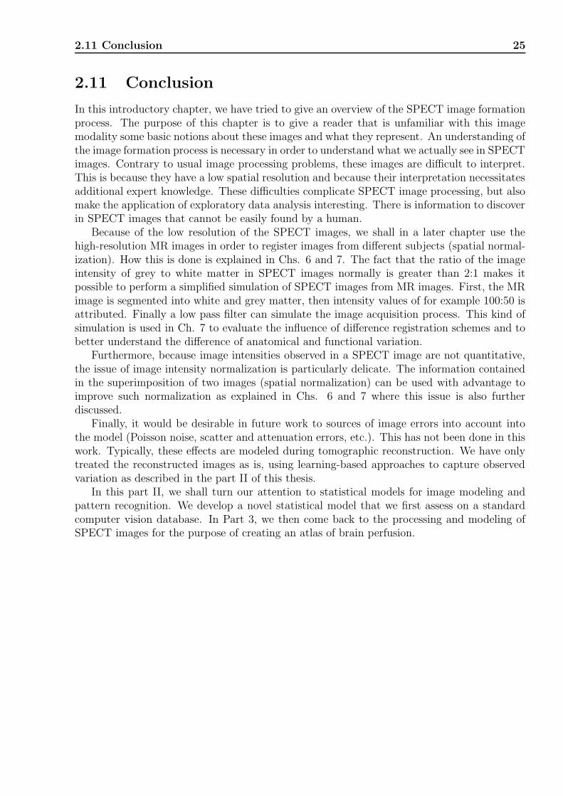
2.11 Conclusion 25
2.11 Conclusion
In this introductory chapter, we have tried to give an overview of the SPECT image formationprocess. The purpose of this chapter is to give a reader that is unfamiliar with this imagemodality some basic notions about these images and what they represent. An understanding ofthe image formation process is necessary in order to understand what we actually see in SPECTimages. Contrary to usual image processing problems, these images are difficult to interpret.This is because they have a low spatial resolution and because their interpretation necessitatesadditional expert knowledge. These difficulties complicate SPECT image processing, but alsomake the application of exploratory data analysis interesting. There is information to discoverin SPECT images that cannot be easily found by a human.
Because of the low resolution of the SPECT images, we shall in a later chapter use thehigh-resolution MR images in order to register images from different subjects (spatial normal-ization). How this is done is explained in Chs. 6 and 7. The fact that the ratio of the imageintensity of grey to white matter in SPECT images normally is greater than 2:1 makes itpossible to perform a simplified simulation of SPECT images from MR images. First, the MRimage is segmented into white and grey matter, then intensity values of for example 100:50 isattributed. Finally a low pass filter can simulate the image acquisition process. This kind ofsimulation is used in Ch. 7 to evaluate the influence of difference registration schemes and tobetter understand the difference of anatomical and functional variation.
Furthermore, because image intensities observed in a SPECT image are not quantitative,the issue of image intensity normalization is particularly delicate. The information containedin the superimposition of two images (spatial normalization) can be used with advantage toimprove such normalization as explained in Chs. 6 and 7 where this issue is also furtherdiscussed.
Finally, it would be desirable in future work to sources of image errors into account intothe model (Poisson noise, scatter and attenuation errors, etc.). This has not been done in thiswork. Typically, these effects are modeled during tomographic reconstruction. We have onlytreated the reconstructed images as is, using learning-based approaches to capture observedvariation as described in the part II of this thesis.
In this part II, we shall turn our attention to statistical models for image modeling andpattern recognition. We develop a novel statistical model that we first assess on a standardcomputer vision database. In Part 3, we then come back to the processing and modeling ofSPECT images for the purpose of creating an atlas of brain perfusion.

26 Introduction to SPECT Imaging

Part II
Appearance-Based, ProbabilisticImage Modeling


Chapter 3
State of the art
3.1 Introduction, overview
We have been interested in using appearance-based models for modeling images. The methodsfor such modeling have been applied with much success since the nineties, beginning with theworks of Sirovich and Kirby [195] for compression of face images and Turk and Pentland [213]for recognizing faces in images. These methods are based on a Karhunen-Loeve transforma-tion of the observed images. This transformation is found by solving the eigenproblem forthe covariance matrix of representative images, which yields the name of the method: eigen-faces. Since the eigenvalues to this eigenproblem can be interpreted as the variances along thecorresponding eigenvector, one retains the principal energy of the representative images bykeeping only information along the eigenvectors of the highest eigenvalues. This is called prin-cipal component analysis and is effectively a dimension reduction technique since the retainedeigenvectors describe a subspace of the original observation space.
We thus have an alternative to the classic approach of modeling objects as seen in images.Instead of extracting features and modeling these, one instead tries to capture interestingstructure in the data using a dimension reduction technique directly on the entire image.These methods are therefore called global methods. The work of Turk and Pentland inspiredmany new ideas in this domain: other applications (object detection, object tracking in imagesequences), other techniques for dimension reduction (linear and non-linear), behavior of objectappearance (object rotation, illumination changes), additional modeling (robust, subspacemodeling) as well as probabilistic bases for such models.
Two leaps forward in this domain are particularly relevant to our work. The first is thework of Murase and Nayar [163], where the authors introduced a non-linear modeling of theimages in the subspace spanned by the eigenvectors. This modeling permitted the authorsto boost the performance of recognizing objects (and object pose). The second is the workof Moghaddam and Pentland [162], where a complete probabilistic model based on principalcomponent analysis is developed. This complete model permitted the authors to boost, amongothers, face detection performance. Another major contribution came from Black and Jepson[13]. They introduced robust estimation techniques that made the models robust towardocclusions and cluttered backgrounds, which is often encountered in natural (outdoor) scenes.
Because of the central position of these methods in our work, we devote a section to theeigenfaces era where we review the chronological developments associated with these models.We then proceed by presenting an overview of dimension reduction techniques in general,before other important developments relative to our work - robust noise modeling and non-

30 State of the art
parametric density estimation - are discussed at the end of this chapter. Global appearancemodeling, principal component analysis, non-parametric density modeling and robust noisemodeling are the building blocks of the model presented in the next chapter.
Note that in this part, we are not concerned with the creation and application of a brainperfusion atlas. We shall see in part III how appearance-based models can be used for thispurpose. The model we develop in Ch. 4 is quite general in scope. In order to illustrate theadvantages and the versatility of this model, we perform experiments on a standard computervision database in Ch. 5.
3.2 General background
Before describing the eigenfaces methods in detail, we will touch on some of the ideas thatlie behind the approaches we have pursued in our work. These ideas are of a more generalnature. Concrete and specific cases follow in the next section. For the sake of clarifying thevocabulary, we begin with a definition of the word appearance.
3.2.1 Appearance
What is the appearance of an object? Cambridge advanced learner’s dictionary provides thefollowing definition: the way a person or thing looks to other people. Appearance is the visibleaspect of an object or a person. This aspect depends on the object itself and how it reflectslight. The appearance of an object, as we capture it with a camera, is therefore a combinedeffect of object shape, reflectance properties, pose, as well as illumination conditions. Theappearance is a notion that is related to an object in its totality, e.g. the appearance of a face,a hand, a car etc. We therefore consider an appearance to be a global property of the object.However, we often distinguish between local and global object appearance in images. By globalappearance we understand the appearance of the object in its entirety, by local appearance weunderstand the appearance of a part of the object.
3.2.2 Representing appearance
In computer vision, we try to teach computers how to interpret scenes and recognize objectsand people from their appearances1. How can we represent, model and interpret appearance?When we point a camera at an object, we obtain a matrix of pixels, each with a particular grayvalue (or even three values for a color camera). We can think of this two-dimensional imageas a surface in a three dimensional space, where the two first axes are the pixel coordinatesand the third axis is the gray value. To interpret the image, we need to analyze this surface.Such interpretation often relies on recognizing an object in the image, i.e. pattern recognition.To do this, we need to find a way of representing images mathematically. We can distinguish“classical” methods and appearance-based methods. The classical approaches are based ongeometrical object models and the analysis of local image characteristics such as edges andcorners (i.e. local appearances, features). The image is represented by a set of features. Theseapproaches are well suited for the analysis of artificial (human made) environments. Anotherclass of more recent approaches are the so-called appearance-based approaches and are based
1Many people consider that one should not judge people by their appearance. As long as computers remainimpersonal, this is of no big concern to computer scientists.

3.2 General background 31
on techniques for learning the appearance of an object from examples. These approachesproceed in two steps:
• The image is coded into a vector with the same number of elements as there are pixelsin the image, say D. The image is therefore coded as a point in the vector space R
D.
• A set of example images (learning images) form together a cloud of points in this space.This cloud is described in mathematical terms, typically using a model.
A simple model could, for example be the representation an object by its average appearance.A simple form for interpretation could then be to compare a new image to this average imageby calculating the euclidean distance between the two points in R
D - this is the well knowntemplate matching technique. More sophisticated techniques use dimension reduction tech-niques and statistical modeling, which are the methods that we have chosen in this thesis.The term appearance-based might seem a bit unclear since any computer vision system is, insome sense, appearance-based. The term however, refers more to the ability of these meth-ods to learn models from appearances than the fact that the signal we are processing is anappearance.
In Part III of this thesis we use appearance-based models to model three-dimensionalSPECT images. The “scene” or “object” we are looking at is the distribution of radiomarkersin the brain cells. The appearance of this scene is a hyper-surface in a 3+1 dimensionalspace. This is clearly a much wider interpretation of the term appearance than the definitiongiven above, but both classical approaches and appearance-based methods can also be used tointerpret three-dimensional images. An explicit geometrical model (whether it exists or not)is not known to us and we would like to employ a method that can learn the model fromexamples. This motivates the use of appearance-based modeling.
3.2.3 Structure in data
The ability to recognize complex patterns embedded in large quantities of information (suchas images), is a remarkable faculty of animals in general and the human in particular. Therenowned biologist Konrad Lorenz described how in one week he became capable of distin-guishing between the plentiful families of colorful fishes that he encountered when scubadivingbetween coral reefs in Florida [142]. The ability to recognize nutritious fruits, recognize prayand predators and their patterns of movement, etc. is probably a very important element inincreasing the chances of a species to survive in the game of nature where mutation and selec-tion play a decisive role. The important thing about recognizing patterns is that it improvesthe ability to predict the behaviour of, say, predators. Now, why would one like to teach suchcapabilities to computers? The first answer is curiosity. Humans are interested in recursivelyunderstanding how they themselves recognize patterns - recognizing how a human recognizesa pattern. Reproducing pattern recognition under controlled conditions on computers is apowerful way for doing this. The answer is, one could say, quite biologically inspired: humanscannot help themselves for searching new patterns in data since they have always done so. Thesecond answer is related to the first, we would like to use the calculating power of a computerto recognize patterns in quantities of data that surpasses the capabilities of the human brain.Even though humans are excellent pattern recognizers, the limits are soon encountered whentrying to understand and predict complex systems: sea and air dynamics, human influence onthe nature, social behaviour, how the brain functions etc. If we find principled ways of learn-ing patterns, we bear hope that this can be used to better understand such complex systems.

32 State of the art
A third answer to the above question is more pragmatic, but probably the one that makespattern recognition research thrive the most: the goal of “making robots and computers hearand see”. This has indeed many applications such as the replacement of tedious or dangerousprocesses which are done, or cannot be done, by man today (spam filtering, maintenance tasksin dangerous environments, etc.).
The problem of recognizing patterns is one of finding structure in data. Without structure,we cannot predict anything. Structure in the data can be [30]:
• Linear: correlations between variables
• Non-linear: clustering or multimodality, skewness or kurtosis (non-Gaussianity), discon-tinuities and, in general, concentration along nonlinear manifolds.
If we reason in terms of points in high dimensional spaces, we can find such structures auto-matically, using methods that are generally denoted dimension reduction techniques. For themodeling of high dimensional data, such techniques are, on one hand necessary, and on theother hand possible. First, dimension reduction is necessary because of a phenomenon calledthe curse of dimensionality (also empty space phenomenon). This refers to the fact that, in theabsence of simplifying assumptions, the sample size needed to estimate a function of severalvariables to a given degree of accuracy grows exponentially with the number of variables. Thisis because the hyper-volume of such spaces are indeed vast (see for example [58, 72, 110] or[30]). Second, dimension reduction is possible because many physical phenomena are indeedgoverned by a few variables. Our measurement systems (e.g. microphone, CCD or gammacamera) do not measure these directly but instead measure a set of redundant variables. Thisredundancy may be caused by:
• Variation in the variables that is smaller than the measurement noise. These are thereforeirrelevant.
• Variables that are correlated (either through linear combinations or other functionaldependencies).
As an example, consider a set of appearances that are representative of a particular object.These form a cloud of points in the image space, R
D (observation space). This image spacespans all possible gray value combinations of pixels. It is therefore clear that the cloud ofappearances of the object will only occupy a lower dimensional subspace (manifold) in theobservation space. This is the subspace that we try to determine using dimension reductiontechniques. Some illustrative examples of low-dimensional manifolds embedded in spaces ofhigher dimensions are shown in Fig. 3.1.
In conclusion, dimension reduction techniques provide a way of automatically learningmodels from examples that can be used for recognition and prediction. These techniques findstructure in data. In practice, principal component analysis (PCA) is the single most importantsuch technique [30]. We shall discuss PCA in Sec. 3.3 and we review other dimension reductiontechniques used in visual modeling in Sec. 3.4. Dimension reduction is necessary to allow forprobabilistic modeling because of the curse of dimensionality.
3.2.4 Modeling for classification and detection
All problems of pattern recognition can in general be reduced to a problem of classification:assigning a semantic class label to a pattern. An example of such classification is the task of

3.2 General background 33
-1
-0.8
-0.6
-0.4
-0.2
0
0.2
0.4
0.6
0.8
1
-10 -5 0 5 10
(a)
-6-4
-2 0
2 4
6 -1-0.8-0.6-0.4-0.2 0 0.2 0.4 0.6 0.8 1
-1-0.8-0.6-0.4-0.2 0 0.2 0.4 0.6 0.8 1
(b)
-10 -5 0 5 10-10
-5
0
5
10
-1-0.8-0.6-0.4-0.2
0 0.2 0.4 0.6 0.8
1
(c)
Figure 3.1: Examples of low-dimensional manifolds embedded in higher dimensional spaces:(a) one-parametric manifold in 2-D (dimensions), (b) one-parametric manifold in 3-D, and (c)two-parametric manifold in 3-D.
identifying a person from a passphoto (also called recognition). However, for the particularproblem of deciding whether a person is present in an image or not, the term detection isgenerally used. The detection problem is often more difficult to solve than the recognitionproblem. This is because we do not in general have a specific model for the non-person class.Methods that learn from examples do not deal easily with this problem because it is difficult toobtain a complete sample of all non-person appearances (though such methods exist [80]). Onepossible way to deal with this problem is to build a complete, realistic and generic model ofthe object class and then base the detection on thresholding some similarity measure betweenthe model and the observation. The disadvantage of such an approach over discriminatingapproaches is that we have to model many aspects that may be irrelevant for detection orclassification. An advantage of generic modeling is however that training is reduced to aset of images of the object class. If the modeling is correct, there is hereby no loss in thediscriminative performance.
In Part II of this thesis, where we try to model normal brain perfusion, a generic modelis preferable because of the difficulty to define what is abnormal brain perfusion. An exact,realistic model is furthermore necessary in order to characterize abnormal perfusion patterns.A famous citation, often mentioned when discussing class and non-class distributions, is theopening sentence of Leo Tolstoy’s Anna Karenina: “All happy families are alike; each unhappyfamily is unhappy in its own way.”
3.2.5 Probabilistic modeling
As in many physical problems, exact mathematical modeling of object appearance in realscenes is not feasible, however stochastic modeling has been applied with much success inmany domains. The key to a statistical approach is to have probability models that capturethe essential variability and yet are tractable. In a statistical approach, we can model uncertain(i.e. random) effects. Other potential advantages of using probabilistic models are:
• They provide principled methods for model estimation and comparison, as well as clas-sification of new observations (e.g. Maximum Likelihood principle and, in particular,Bayesian inference).
• They provide a natural way of combining different measurements (information fusion).

34 State of the art
• There are principled ways for dealing with missing data in multivariate models (e.g. bymarginalizing over the missing observations).
• Statistical decision theory can be employed (i.e. hypothesis testing).
• We can generate new samples from the model.
A word of moderation is required however, since statistical assumptions are often approx-imative. This means that many of the above mentioned advantages of statistical modelingare no longer valid, in which case we return to “random thresholding”. However, even incases where model assumptions are clearly wrong, statistical approaches are often attractivebecause (1) they provide a framework for modeling and interpretation, and (2) statisticiansand pattern recognitioners “feel” better when their method has at least some relation to wellestablished mathematical principles. This is indeed a difficult issue!
3.2.6 Probability density estimation
In pattern recognition we are interested in developing methods that learn a model (e.g. ofobject appearance) from observations. For a probabilistic model this is the same as estimatingthe probability density function. The estimation can be done based on different principles suchas least-squares minimization, maximum likelihood principle, maximum-a-posteriori principle,Bayesian inference, minimum description length principle or structural risk minimization [58,12, 72, 217]. High accuracy of this estimation is indeed important to obtain good recognitionperformance. For the high dimensional data that we are considering in this thesis, densityestimation is not possible without using dimension reduction techniques (because of the emptyspace phenomenon).
The model that we have chosen will be presented in the next chapter. On the theoret-ical level, this thesis has been less concerned with the estimation of the density function ofthis model than with making extensions to the model when considering that the model isapproximately justified (sufficiently well estimated). For this we needed to develop a newalgorithm (presented in Ch. 4). The importance of this algorithm is that it makes it possibleto make inferences under the extended model. For model estimation we have used principalcomponent analysis (PCA - Sec. 3.3.1). This choice was motivated by the development ofprobabilistic PCA (PPCA - Sec. 3.3.5), which provides the link between a complete multi-variate probabilistic model, dimension reduction (by PCA) and maximum likelihood densityestimation.
3.2.7 Partial conclusion
After this section on general aspects of appearance, pattern recognition, probabilities and high-dimensional data, we shall now become more concrete and describe the eigenface methods indetail.
3.3 The Era of eigenfaces
3.3.1 Principal component analysis (PCA)
In most appearance-based models, principal component analysis (PCA) is still the basicworkhorse. In fact, appearance-based techniques have probably gained a lot of popularity

3.3 The Era of eigenfaces 35
because of their conceptual simplicity combined with readily available algorithms of low com-putational complexity for performing PCA. PCA in its original form is not based on any modeland is therefore a method for exploratory data analysis. We can summarize PCA as follows.Let yJj=1 be J samples from a stochastically distributed variable of D components. If wedenote the mean-free sample matrix by Y = [y1−µ . . .yJ−µ], we can estimate the covarianceof the data as:
Σy =1
JY Y T .
As with any symmetric real matrix, we can diagonalize the covariance matrix (or the estimatethereof) by solving the eigenproblem and we obtain:
Σy = WΛW T = [w1 · · ·wD]
λ1 0. . .
0 λD
wT1...
wTD
, (3.1)
where Λ is a diagonal matrix of eigenvalues and W is a D×D rotation matrix of eigenvectors(W T W = I). This decomposition has several interesting properties (see for example [58, 72]or [12]):
• The eigenvectors define a new coordinate basis into which the original samples can betransformed as (Karhunen-Loeve transformation): x = W T (y − µ). The covariance ofthe transformed variable is Σx = W TΣyW = Λ since the eigenvectors are orthonor-mal. This means that the components of the transformed variable are decorrelated.Furthermore, if the distribution of y ∼ p(y) is Gaussian, then the components of x
are statistically independent. We can also think of this transformation as a projectionoperator which projects the observation vector into the transformed space.
• The eigenvalues are the variances (signal energies) of the observation variable along thecorresponding eigenvectors. The eigenvectors that belong to the highest eigenvalues arethe principal components of the data.
• Principal component analysis is a signal compression (or dimension reduction) schemewhere we define a truncated version of the Karhunen-Loeve transformation defined above:If we reorder the eigenvectors and eigenvalues so that λ1 ≥ λ2 ≥ . . . ≥ λD we obtain anoptimal signal compression scheme in the least squares sense by defining the transforma-tion W Q = [w1 · · ·wQ], where Q < D. Compression is done by projecting the originalsignal into the eigenspace or subspace as
xQ = W TQ(y − µ). (3.2)
The reconstruction of the signal is then defined as:
yQ = W QxQ + µ. (3.3)
This compression is lossy and the residual of the reconstructed signal is defined as:
e = y − yQ. (3.4)
The compression has the property that it minimizes the square sum reconstruction erroreT e, and retains a percentage of the original signal energy as:
∑Qq=0 λq
∑Dq=0 λq
. (3.5)
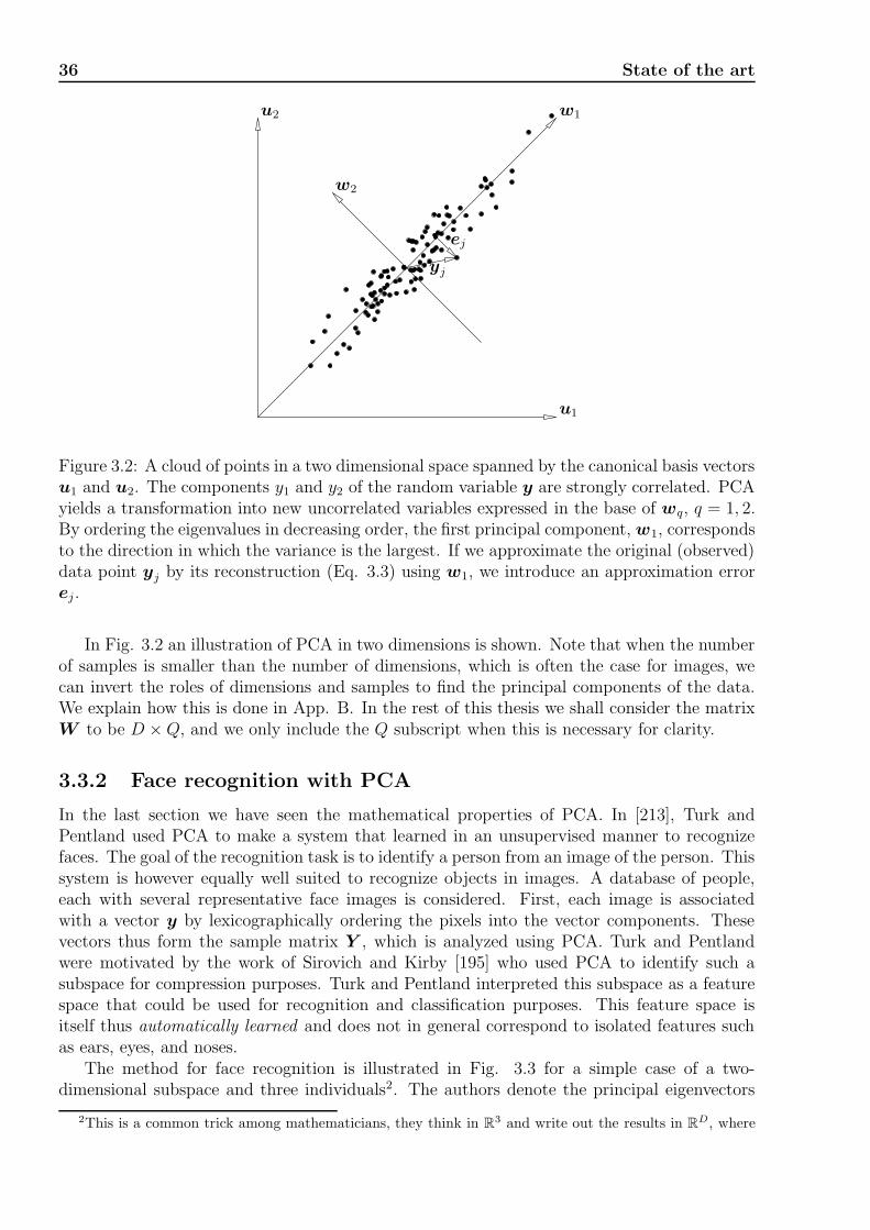
36 State of the art
w1
w2
ej
yj
u1
u2
Figure 3.2: A cloud of points in a two dimensional space spanned by the canonical basis vectorsu1 and u2. The components y1 and y2 of the random variable y are strongly correlated. PCAyields a transformation into new uncorrelated variables expressed in the base of wq, q = 1, 2.By ordering the eigenvalues in decreasing order, the first principal component, w1, correspondsto the direction in which the variance is the largest. If we approximate the original (observed)data point yj by its reconstruction (Eq. 3.3) using w1, we introduce an approximation errorej.
In Fig. 3.2 an illustration of PCA in two dimensions is shown. Note that when the numberof samples is smaller than the number of dimensions, which is often the case for images, wecan invert the roles of dimensions and samples to find the principal components of the data.We explain how this is done in App. B. In the rest of this thesis we shall consider the matrixW to be D ×Q, and we only include the Q subscript when this is necessary for clarity.
3.3.2 Face recognition with PCA
In the last section we have seen the mathematical properties of PCA. In [213], Turk andPentland used PCA to make a system that learned in an unsupervised manner to recognizefaces. The goal of the recognition task is to identify a person from an image of the person. Thissystem is however equally well suited to recognize objects in images. A database of people,each with several representative face images is considered. First, each image is associatedwith a vector y by lexicographically ordering the pixels into the vector components. Thesevectors thus form the sample matrix Y , which is analyzed using PCA. Turk and Pentlandwere motivated by the work of Sirovich and Kirby [195] who used PCA to identify such asubspace for compression purposes. Turk and Pentland interpreted this subspace as a featurespace that could be used for recognition and classification purposes. This feature space isitself thus automatically learned and does not in general correspond to isolated features suchas ears, eyes, and noses.
The method for face recognition is illustrated in Fig. 3.3 for a simple case of a two-dimensional subspace and three individuals2. The authors denote the principal eigenvectors
2This is a common trick among mathematicians, they think in R3 and write out the results in R
D, where

3.3 The Era of eigenfaces 37
y − µ
x
Ω1
w1
w2
Ω2
Ω3
Figure 3.3: A geometric illustration of the subspace (“face space”) for two eigenvectors, w1
and w2 (“eigenfaces”), and three known classes (individuals). New images are projected intothe subspace and associated with the nearest class in this subspace.
“eigenfaces”, which span a subspace they denote “face space”. This face space is then usedfor recognition. A new image is transformed (projected) into the face space and classified tothe class that has the closest projections. Several cases are distinguished: by looking at theresidual - or the reconstruction error - they first decide whether the image is a face or not(detection). A large residual means the distance from face space is far. This is the distancethat Moghaddam later denotes distance from feature space (DFFS). Second, if an image is farfrom any class, but close to the face space, it is considered to be an unknown face which caneventually be added to the database. Third, if an image is close to face space and close to aface class, the observation is associated with that class.
3.3.3 Non-linear subspace modeling
Whereas Turk and Pentland modeled every class (person) in the subspace with a Gaussian dis-tribution, Murase and Nayar [163] introduced a more complex parametric subspace model forobject recognition. In an experiment, they acquired images of the same object under differentviews (poses): they placed an object on a turntable and obtained an image at every 5 degrees.This was repeated for several objects. Two types of eigenspaces were built: one for objectidentification, where all the images were included in the learning set, and another subspacefor each object intended for pose classification. They noticed that the rotated objects formedparticular spiral-like patterns in the subspace and modeled these using cubic spline interpola-tion, see Fig. 3.4. The authors denoted this model parametric eigenspace representation. Poseclassification consisted of projecting the observation into the subspace and finding the closestpoints on the manifold described by the parametric function.
The method is non-linear, but we can think of the model as an initial linear dimensionreduction followed by non-linear modeling. This is done in many other dimension reduc-tion techniques as well, where an initial PCA reduction is followed by some other methods(described in Sec. 3.4). We note that in [31], Chalmond and Girard develop a method for
the size of D is not even mentioned.
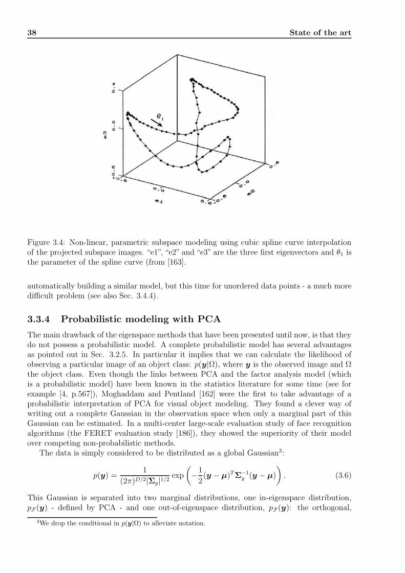
38 State of the art
Figure 3.4: Non-linear, parametric subspace modeling using cubic spline curve interpolationof the projected subspace images. “e1”, “e2” and “e3” are the three first eigenvectors and θ1 isthe parameter of the spline curve (from [163].
automatically building a similar model, but this time for unordered data points - a much moredifficult problem (see also Sec. 3.4.4).
3.3.4 Probabilistic modeling with PCA
The main drawback of the eigenspace methods that have been presented until now, is that theydo not possess a probabilistic model. A complete probabilistic model has several advantagesas pointed out in Sec. 3.2.5. In particular it implies that we can calculate the likelihood ofobserving a particular image of an object class: p(y|Ω), where y is the observed image and Ωthe object class. Even though the links between PCA and the factor analysis model (whichis a probabilistic model) have been known in the statistics literature for some time (see forexample [4, p.567]), Moghaddam and Pentland [162] were the first to take advantage of aprobabilistic interpretation of PCA for visual object modeling. They found a clever way ofwriting out a complete Gaussian in the observation space when only a marginal part of thisGaussian can be estimated. In a multi-center large-scale evaluation study of face recognitionalgorithms (the FERET evaluation study [186]), they showed the superiority of their modelover competing non-probabilistic methods.
The data is simply considered to be distributed as a global Gaussian3:
p(y) =1
(2π)D/2|Σy|1/2exp
(
−1
2(y − µ)TΣ−1
y (y − µ)
)
. (3.6)
This Gaussian is separated into two marginal distributions, one in-eigenspace distribution,pF(y) - defined by PCA - and one out-of-eigenspace distribution, pF(y): the orthogonal,
3We drop the conditional in p(y|Ω) to alleviate notation.

3.3 The Era of eigenfaces 39
isotropic noise distribution. Since the latter distribution is not known, it is estimated aspF(y) by considering the noise orthogonal to the subspace to be isotropic. The separation intopF and pF is equivalent to a partitioning of the observation space. The following estimationof the complete Karhunen-Loeve transformation is then obtained:
p(y) =
[
exp(−1
2xTΛ−1
Q x)
(2π)Q/2|ΛQ|1/2
]
·
exp
(
−eT e2σ2
)
(2πσ2)(D−Q)/2
= pF(y)pF (y), (3.7)
where ΛQ is the truncated diagonal matrix of eigenvalues, x is the projection of the image intothe subspace (Eq. 3.2) defined by the eigenvectors W Q, e = y −W Qx is the residual vectorfrom Eq. 3.4, and σ is the estimated, isotropic noise variance in the orthogonal directions ofthe eigenspace. The first term is associated with the Mahalonobis distance xTΛ−1
Q x which theauthors term Distance in Feature Space (DIFS). The second term is computable because thenoise is considered to be isotropic in the orthogonal space: We can ignore the exact directionof the residual, all that matter is that it lies in this orthogonal space. To see this we write thedistribution in Eq. 3.7 as:
y ∼ N (µ,Σy), where Σy = [W QW D−Q]
ΛQ 0σ2
. . .
0 σ2
[W T
Q
W TD−Q
]
. (3.8)
Here, the eigenvectors of the orthogonal space, W D−Q, do not need to be computed4: theMahalonobis distance in the complementary space can be calculated directly from the recon-struction errors (residuals) as eT e
σ2 (Eq. 3.7). The authors call this distance the Distance fromFeature Space (DFFS). The DFFS is particularly important for detection, which necessitatesthe calculation of the likelihood of an observation. However, it can be ignored for recognition[161] (verified in personal communication). Fig. 3.5 illustrates the distances DIFS and DFFS.
The noise variance of the “noise-space” is estimated by minimizing the Kullback-Leiblerdivergence between the true and estimated densities, which yields:
σ2 =1
D −QD∑
q=Q+1
λq. (3.9)
In practice, many of these eigenvalues may not be available. One possibility, as proposed byMoghaddam and Pentland, is to estimate these by fitting a 1/f function to the spectrum ofcomputed eigenvalues (which are declining).
Note that the separation of the Gaussian into the product of two marginal distributionsis different from a model where the systematic part and the noise have been separated, as isthe case in “true” probabilistic PCA and in factor analysis. In this kind of probabilistic PCAthe noise and the systematic part are treated equally. We shall come back to this point in thenext section.
3.3.5 Probabilistic Principal Component Analysis (PPCA)
The so-called probabilistic principal component analysis (PPCA) model that is based on thefactor analysis model was developed by Tipping and Bishop [212, 211] and independently by
4Often these eigenvectors cannot be calculated because the sample size is too small.

40 State of the art
y − µ
x
w1
w2
w3
DFFS
DIFS
pF(y|Ω)
Figure 3.5: In illustrative example of the two distances DFFS and DIFS (see the text). Thesubspace is spanned by two principal components w1 and w2, the complementary space isspanned by w3. The inspace distribution of the object is drawn as a dotted ellipse. For theobserved vector y both DFFS and DIFS are evaluated to determine whether an object is closeto its class distribution or not.
Roweis [188, 189] (under the name of sensible PCA). This model has not to our knowledgebeen used for face modeling, but has been applied to build class hierarchies of objects [57] aswell as for analysis and visualization of multispectral data [11]. The PPCA model has theadvantage that it leaves more room for interpretation and extensions than the model proposedby Moghaddam and Pentland. We now describe the PPCA model and will later describe itsrelation to the model of Moghaddam and Pentland.
The model is a linear latent variable model of the form
y = Wx + µ + ε (3.10)
where a new random variable has been introduced: theQ dimensional latent variable (subspacevariable), x. The components of this variable are considered to be identically and independentlydistributed (i.i.d) as a Gaussian with unit variance, x ∼ N (0, IQ). The noise distribution isalso Gaussian and isotropic, ε ∼ N (0, σ2ID). Here, the D × Q dimensional factor loadingsor generation matrix, W is in general not the eigenvectors of the covariance matrix, but it isorthogonal. Under the model assumptions we can calculate the following distributions ([212]and our calculations):
• The distribution of the observation is Gaussian, y ∼ N (µ,Σy), with the variance (seefor example [4, p.553]):
Σy = σ2ID + WW T . (3.11)
If we let W Q = W and denote by W D−Q a matrix of vectors that spans the spacethat is orthogonal to the space defined by W , we can rewrite the variance as (analog to

3.3 The Era of eigenfaces 41
Eq. 3.8):
Σy = [W QW D−Q]
σ21 + σ2 0
. . .
σ2Q + σ2
σ2
. . .
0 σ2
[W T
Q
W TD−Q
]
, (3.12)
where σq, q = 1 . . .Q are the variances induced by the systematic part of the model, Wx.
• The conditional distribution of the observation given the latent variable is p(y|x) =N (Wx + µ, σ2ID). This is also the key motivation for the model: the components ofthe observed image y are conditionally independent given the latent subspace variable x.
• The posterior distribution of the latent variable given the observation is Gaussian withp(x|y) = N (µx,Σx|y), where
µx = (σ2IQ + W T W )−1W T (y − µ), (3.13)
andΣx|y = σ2(σ2IQ + W T W )−1.
Note that the last term in Eq. 3.13 is the same as the PCA projection, Eq. 3.2. InPPCA the expectation of the posterior, µx, is indeed the most appropriate choice forprojecting an observation into the subspace. We shall discuss in depth this kind ofposterior distribution under more general model assumptions in the next chapter.
In [212], Tipping and Bishop develop the exact maximum-likelihood estimate of this model,when the covariance Σy is estimated by the sample covariance matrix Σy. The resultingestimators are:
• The mean vector
µ =1
J
J∑
j=1
yj. (3.14)
• The generation matrixW = UQ(ΛQ − σ2IQ)1/2R, (3.15)
where the Q column vectors in the D×Q matrix UQ are the eigenvectors of the sample
covariance matrix Σy, with corresponding eigenvalues in the Q×Q diagonal matrix ΛQ.The matrix R is an arbitrary Q × Q orthogonal rotation matrix. This arbitrariness isexplained by an ambiguity in the model Eq. 3.10: the distribution p(y) is invariant torotation of the generation matrix, i.e. the model variance does not change (Eq. 3.11).
• The noise variance
σ2 =1
D −QD∑
q=Q+1
λq, (3.16)
where λq+1, . . . , λd are the smallest eigenvalues of Σy. This maximum likelihood estimateis exactly the same as the estimate found by Moghaddam and Pentland by minimizingthe Kullback-Leibler divergence, Eq. 3.9.

42 State of the art
With these estimates, the distribution of observations, p(y), becomes exactly the same asthe distribution found by Moghaddam and Pentland (i.e. with the estimated generation matrixEq. 3.15, the global covariance matrix Eq. 3.12 becomes equal to the global covariance matrixin Eq. 3.8). We can thus explain the relation between the two models: since Moghaddam andPentland do not model the subspace variable as an independent random variable, we obtaintheir model from the PPCA model as the marginal distribution at the maximum likelihoodestimate Θ = (W , µ, σ) of the joint distribution p(y,x) as:
p(y)|Θ =
∫
p(y,x)|Θdx.
As an illustrative example, consider an object whose appearance only changes in the lowerregion of the image. Furthermore, consider that both models could identify this region as theprincipal subspace with, say, the same number of principal axes as there are pixels in thisregion. Now, whereas the model of Moghaddam and Pentland only considers the noise to bepresent in the upper region of the image (the orthogonal, complementary space), the PPCAmodel considers an additive noise everywhere in the image. This is also seen in the Eqs. 3.12and 3.8. The relation between these two models has to our knowledge not been clearly statedin the literature, however, Moghaddam points out in [161] that their model is a special caseof the PPCA model.
3.3.6 Analytical PCA
The experiments of Murase and Nayar [163], described in Sec. 3.3.3, showed that the distri-bution of rotated objects formed characteristic clouds in the subspace. Several authors havetherefore investigated the exact relationship between the subspace distribution (as found byPCA) of appearances issued from controlled changes such as illumination changes [9, 187],rotation of images [215] and panoramic images [113]. These studies undermine the idea thatthe images of objects have intrinsic dimensions that are largely inferior to the dimension of theobservation space R
D. In particular, Uenohara and Kanade [215] showed that the distributionin subspace of rotated images of an object will lie on a one-dimensional circular-like curve,i.e. the projections of the learning images into a two-dimensional subspace spanned by twosuccessive eigenvectors form circles. We have used this knowledge to design experiments withlearning set data that form non-linear, non-Gaussian subspace distributions (Ch. 5).
3.3.7 Partial conclusion
We have presented a detailed and chronological tour of PCA-based methods that have beenused for modeling objects and faces in the last decade. The tour was rounded off with theprobabilistic PCA model, which establishes a probabilistic framework for appearance-basedmodels. These particular methods were presented because they form the natural ancestry ofthe model developed in this work. We now review other methods that have been, or can be,used for appearance modeling. We then come back to some recent developments concerningrobust noise modeling in the PPCA framework.
Before continuing, let us just mention a little curiosity. Whereas many researchers tryto find compact manifolds that capture facial variations, a complementary approach for vi-sualizing high-dimensional variables (for exploratory purposes) was developed by Chernoff5.
5See for example http://people.cs.uchicago.edu/~wiseman/chernoff/

3.4 Other dimension reduction techniques 43
The method is based on generating drawings of faces. Since humans are highly specialized inrecognizing faces and facial expressions, Chernoff made a mapping between a ten-dimensionalsubspace onto different facial features such as size of the nose, eccentricity of the head, dis-tance between eyes etc. The idea is that when mapping the (high-dimensional) samples ontothese faces, a human could be capable of recognizing structure (clusters) in the data. Wedo not know if someone has tried (or succeeded) in creating photorealistic Chernoff-faces bylearning a subspace from training samples. This could certainly be envisaged by means ofappearance-based models!
3.4 Other dimension reduction techniques
We have explained in Sec. 3.2.3 why dimension reduction is necessary and why it is (often)possible. In Sec. 3.3 we saw our method of choice, PCA, in action. In this section we providea brief outline of other dimension reduction techniques in image modeling. These can bedivided into linear and non-linear methods. Let us begin by providing a formal definition ofthe problem and what the intrinsic dimension of a phenomenon is.
3.4.1 Problem statement
The problem of dimension reduction can be stated as follows; We have a given sample ofobservations, say yjJj=1, of D-dimensional real vectors drawn from an unknown probabilitydistribution. The fundamental assumption that justifies the dimension reduction is that thesample actually lies, at least approximately, on a manifold of smaller dimension than thedata space. The goal of dimension reduction is to find a representation of that manifold (acoordinate system) that will allow us to project the data vectors on it and obtain a low-dimensional, compact representation of the observed data.
3.4.2 The intrinsic dimension of a sample
We have already seen examples of low dimensional manifolds embedded in higher dimensionalspaces in Fig. 3.1. The figure in the middle could for example describe the path of a butterflythrough the room, which is governed by one single independent variable. In practice, manyphenomenon that are governed by a few independent variables will appear as having manymore degrees of freedom due to the influence of a variety of factors: noise, imperfection inthe measurement system, addition of irrelevant variables, etc. The intrinsic dimension of aphenomenon can be defined as the number of independent variables that explain satisfactorilythat phenomenon, e.g. a single independent variable would suffice to describe the butterfly’sflight.
The determination of the intrinsic dimension is central to the problem of dimension re-duction, knowing it eliminates the risk of over- or underfitting. Furthermore, all dimensionreduction techniques take the intrinsic dimension as a parameter. In practice, either a trial-and-error process is necessary, or a regularization term which contains a priori information onthe amount of smoothing to be done must be introduced to determine the intrinsic dimension.The problem is ill-posed because we can fit any data sample given enough free parameters6.In Ch. 8 we determine this dimension by evaluating the generalization error of a detector of
6The problem is closely related to the problem of determining the number of mixtures in density mixturemodels.

44 State of the art
abnormal perfusion patterns. In principal component analysis one often defines a percentageof total variance to be explained by the reduced space, see Eq. 3.5. Minka has proposed anautomatic method to determine the number of principal components in PPCA using Bayesianinference [156]. Other methods have been proposed in [91] and [137].
3.4.3 Classification of techniques
An obvious way of classifying dimension reduction techniques is to distinguish linear andnon-linear methods. Another useful view is proposed by Carreira-Perpinan in [30]:
Hard dimension reduction problems, in which the data have dimensions ranging from hun-dreds to perhaps hundreds of thousands of components (e.g. image modeling), andusually a drastic reduction is sought. PCA is one of the most widespread techniques inmost practical cases.
Soft dimension reduction problems, in which the data is not too high-dimensional (a few tensof components), and the reduction is not very drastic. Typically, the components areobserved or measured values of different variables which have a straightforward inter-pretation. In this class, we find the usual multivariate methods: PCA, factor analysis,linear discriminant analysis, multidimensional scaling etc.
Visualization problems, in which the data doesn’t normally have a very high dimension inabsolute terms, but we need to reduce it to 2, 3 or 4 at most in order to plot it. In thisclass we find projection pursuit, PCA, multidimensional scaling, self-organizing mapsand density networks, as well as interactive programs.
Svensen [201] makes a distinction between generative (probabilistic) and non-generative meth-ods. Other possible distinctions are static/time-dependent, and discrete/continuous data. Weonly consider static, continuous methods, however both generative and non-generative.
3.4.4 Linear methods
Linear models are by far the most applied models in dimension reduction and for many othersignal processing applications as well. Advantages of linear models over non-linear modelsare: mathematical tractability, computationally less expensive, conceptually simpler, and fa-cilitated interpretation. We find again linear models in numerous domains. An interestingunifying view of linear models (PCA, factor analysis, ICA, Kalman filters, hidden Markovmodels,...) can be found in [189], and links between these as graphical models in [164].
Projection pursuit
Projection pursuit is not one single method for linear dimension reduction, but rather a gen-eral framework in which other methods can be seen as special cases. It was introduced asa method for visualization purposes and exploratory data analysis by Friedman and Tukey[63]. Nice introductions can be found in [30] and in [137]. Projection pursuit is an unsu-pervised technique that picks interesting low-dimensional linear orthogonal projections of ahigh-dimensional point cloud by maximizing a objective function called the projection index.This can be computationally tedious. The projection index is a real functional defined onthe space of distributions in R
Q (Q is the subspace dimension). A projection is considered

3.4 Other dimension reduction techniques 45
as being interesting if it contains structure. Because of the following two results, the normaldistribution is considered to be the least interesting (the least structured) density:
• For fixed variance, the normal distribution has the least information (it has the lowestnegative entropy [58, p.631]) among all probability distributions.
• For most high-dimensional clouds, most low-dimensional projections are approximatelynormal [86].
Several projection indices are therefore based on measures of higher order statistics (cumu-lants), the Fisher information or negative entropy. These criteria coincide with the criteriaused for estimating the independent components in independent component analysis (ICA),which we shall see shortly (Sec. 3.4.4). Taking variance as the projection index, the principalcomponents of the data are found. This is why PCA and ICA can be seen as special casesof projection pursuit. Another method for dimension reduction that can be formulated as aprojection pursuit problem is multidimensional scaling [193, 31]. Here, projections are sought,for which the euclidean distances between the projected data remains the same as for the datain the original space. Closely related, Chalmond and Girard [31] uses a an index that conservesthe neighborhood between observations in order to find a linear subspace that is well suitedfor spline interpolation of the projected data. Their method therefore provides an automaticway of obtaining a non-linear model similar to the one of Murase and Nayar [163] (Sec. 3.3.3)in the case of non-ordered observations.
Linear discriminant analysis (LDA)
Linear discriminant analysis (also called Fisher discriminant analysis) is a method for super-vised classification. Here optimal projections of the high dimensional, pre-classified patternsare chosen so that the projected data is optimally separable. The criterion for optimal sepa-rability is a quotient that maximizes the inter-class variance and at the same time minimizesthe intra-class variance. LDA is optimal as a method for dimension reduction when
• the data is linearly separable,
• pre-classified learning samples exist,
• and the samples of each class are normally distributed.
In these cases LDA may indeed be a much more powerful technique for discrimination high-dimensional data than PCA (see also the section on modeling for classification, Sec. 3.2.4).An illustrative example where this is the case is shown in Fig. 3.6. However, only a subspaceof C − 1 dimensions can be found, where C is the number of classes. In [8], Belhumeur et al.showed that Fisherfaces were superior to eigenfaces for recognition. However, this is not alwaystrue as later demonstrated by Martinez et al. in [149]. Furthermore, in practice one oftenapplies LDA after an initial PCA. Another method for finding linear separation planes betweenhigh-dimensional data is the linear support vector machine (SVM) which optimizes a differentobjective function. SVM are more often used in connection with non-linear discrimination(kernel-methods) which we shall see in the next section.

46 State of the art
wPCA
wLDA
u1
u2
Figure 3.6: When the data is pre-classified like here (diamonds and filled boxes represent twodistinct classes), LDA can find low-dimensional projections wLDA, that have higher discrimi-nating power than the projections found by PCA, wPCA.
Factor analysis
Strictly speaking, factor analysis is not considered to be a dimension reduction technique, butit can be used for this purpose. Contrary to the other models in this section, it is a trueprobabilistic model, originally developed in psychology [4] and it is the basis for the PPCAmodel presented in Sec. 3.3.5. The idea in factor analysis is to partition the observation intoan unobserved systematic part and an unobserved error part. This is different from PCA,where directions are sought that explain the observed variance. The model can be written asthe PPCA model in Eq. 3.10:
y = Wx + µ + ε, (3.17)
however with a small but crucial difference: the noise follows a non-isotropic Gaussian dis-tribution ε ∼ N (0,Ψ), with Ψ diagonal. The generation matrix W is in factor analysiscalled the factor loadings. The elements of Ψ are often called the uniquenesses of the model,which points to the unique, independent noise on each observation axis (pixel). The differencebetween PCA (and also PPCA) and factor analysis is given by the following invariances [211]:
• PCA is covariant to rotation of the observation axes, i.e. multiplication from the leftwith an orthogonal matrix R (RT = R−1) in Eq. 3.17 simply leads PCA to find therotated eigenvectors RW .
• Factor analysis is covariant to scaling of the axes, i.e. multiplication from the left witha diagonal matrix A in Eq. 3.17 leads to rescaling of the rows of W and rescaleduniquenesses.
This also means that factor analysis will find directions of correlation (as opposed to those ofhigh variance) between the variables [97]. These directions are independent of the variancewhich is unique to each variable. This is a desirable property for measurements of variablesthat are not believed to have the same noise variance properties (e.g. different mental testscores), but is probably less appropriate for images where we assume the pixel noise variance

3.4 Other dimension reduction techniques 47
to be the same for every pixel. Furthermore, we would expect a rotation of our camera systemto lead to a rotation in the projection axes, not a completely different model.
Another specificity to the factor analysis model is the interpretation of the factor loadingsand the projected variables. Factor analysis was originally used to find latent variables witha meaning, e.g. “intelligence” (psychology), “social class” (sociology7), time curve of the leftheart chamber in dynamic SPECT studies [10], and others. For this it is necessary to interpretthe factor loadings. To facilitate this interpretation it is further (often) necessary to rotatethe axes of W – ideally to obtain directions with a few high loadings. This rotation is calledoblique analysis and much research is dedicated to the development of criteria for this (thevarimax criterion being one of the best known [118]). Oblique analysis can be applied to anyset of axes, also to those found by PCA. This was done for brain SPECT studies in [115], buthas not been an issue in the computer vision community.
Factor analysis is typically used for observation variables of“reasonable”dimensions, say onthe order of 10. However, there have been works on face and digit modeling using mixture offactor analyzers. Such mixtures are possible because the factor analysis model is a probabilisticmodel. We shall come back to this in the next section on non-linear models.
Independent component analysis (ICA)
Independent component analysis is another model for finding linear subspaces that are notnecessarily orthogonal but where the projected variables are statistically independent [117,41, 107, 108]. The motivation behind ICA is the same as for projection pursuit and was firstdeveloped in blind source separation. The idea is that (1) sources of signals that are of interest(objects in images, speakers at a cocktail party) emit stochastic signals that are non-Gaussian(“colored”), and (2) these sources are statistically independent. The observation model isstated as follows:
y = Ax,
where y is the observation, A is a mixing matrix that mixes the statistically independentcomponents of x together. There also exist a “noisy ICA model”
y = Ax + ε,
with additive random noise (also called probabilistic ICA in [7]). However, most researchhas been done on the former due to the difficulty of estimating the latter. Estimating thedemixing matrix A−1 can be quite difficult and several algorithms have been developed forthis [117, 41, 107, 108]. The main properties of ICA are:
• The column vectors of the mixing matrix are (in general) not orthogonal.
• There is no natural ordering of the components (as in PCA).
ICA has been used for modeling local features [236] and for modeling face appearances[6]. Due to contradictory claims in the literature on the relative performance of PCA andICA, Draper et al. [56] recently made a comparative study where they concluded that PCAperformed well, but not as well as ICA. In brain activation studies – both fMRI [150] andPET [183] studies – ICA has been used as an exploratory alternative to model-based analysisin order to find regions with statistically independent temporal behavior.
7For example, Pierre Bourdieu used factor analysis in his famous book “Distinction” [20].
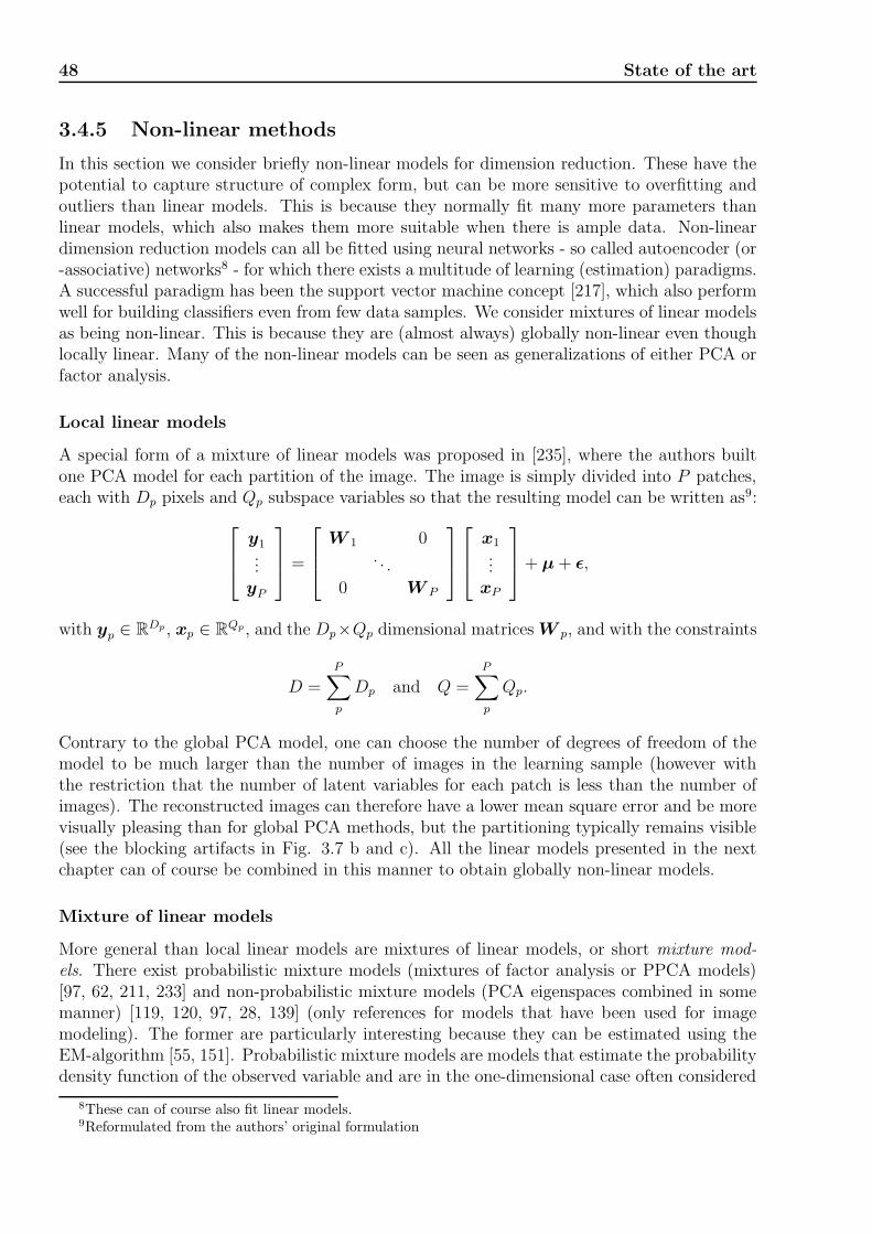
48 State of the art
3.4.5 Non-linear methods
In this section we consider briefly non-linear models for dimension reduction. These have thepotential to capture structure of complex form, but can be more sensitive to overfitting andoutliers than linear models. This is because they normally fit many more parameters thanlinear models, which also makes them more suitable when there is ample data. Non-lineardimension reduction models can all be fitted using neural networks - so called autoencoder (or-associative) networks8 - for which there exists a multitude of learning (estimation) paradigms.A successful paradigm has been the support vector machine concept [217], which also performwell for building classifiers even from few data samples. We consider mixtures of linear modelsas being non-linear. This is because they are (almost always) globally non-linear even thoughlocally linear. Many of the non-linear models can be seen as generalizations of either PCA orfactor analysis.
Local linear models
A special form of a mixture of linear models was proposed in [235], where the authors builtone PCA model for each partition of the image. The image is simply divided into P patches,each with Dp pixels and Qp subspace variables so that the resulting model can be written as9:
y1...
yP
=
W 1 0. . .
0 W P
x1...
xP
+ µ + ε,
with yp ∈ RDp , xp ∈ R
Qp, and the Dp×Qp dimensional matrices W p, and with the constraints
D =P∑
p
Dp and Q =P∑
p
Qp.
Contrary to the global PCA model, one can choose the number of degrees of freedom of themodel to be much larger than the number of images in the learning sample (however withthe restriction that the number of latent variables for each patch is less than the number ofimages). The reconstructed images can therefore have a lower mean square error and be morevisually pleasing than for global PCA methods, but the partitioning typically remains visible(see the blocking artifacts in Fig. 3.7 b and c). All the linear models presented in the nextchapter can of course be combined in this manner to obtain globally non-linear models.
Mixture of linear models
More general than local linear models are mixtures of linear models, or short mixture mod-els. There exist probabilistic mixture models (mixtures of factor analysis or PPCA models)[97, 62, 211, 233] and non-probabilistic mixture models (PCA eigenspaces combined in somemanner) [119, 120, 97, 28, 139] (only references for models that have been used for imagemodeling). The former are particularly interesting because they can be estimated using theEM-algorithm [55, 151]. Probabilistic mixture models are models that estimate the probabilitydensity function of the observed variable and are in the one-dimensional case often considered
8These can of course also fit linear models.9Reformulated from the authors’ original formulation

3.4 Other dimension reduction techniques 49
(a) (b) (c)
Figure 3.7: Examples of a reconstructed image from the COIL database (see Ch. 5). In (a)the image has been reconstructed with 10 eigenvectors, in (b) and (c), the image has beenreconstructed with 9 and 25 patches respectively, each patch with 10 eigenvectors.
as semi-parametric density estimators. Like kernel density estimation methods (see also Sec.3.6), these are therefore potentially capable of modeling (and reducing) any linear and non-linear manifolds. Their estimation remains difficult however since the problem of determiningthe intrinsic dimension is more complex and the EM-algorithm can only find local minima.Mixture distributions are modeled as a sum of linear distributions (typically Gaussian). Forexample a mixture of factor analyzers is given by:
p(y) =K∑
k
πkpk(y), with pk(y) = N (µk,Ψk + W kWTk ),
where each factor is a linear model of the form
y = W kx + µk + εk.
Different variants can then be formulated by fixing the same noise variance across componentsor assuming the noise variance of each component to be isotropic, which yields the mixturePPCA model [211].
Principal curves and principal surfaces
Principal curves and surfaces have been suggested as non-linear generalizations to PCA andwere proposed by Hastie and Stuetzle [92]. Intuitively, a principal curve is a smooth, one-dimensional curve that passes through the “middle” of a cloud of data points in the embeddingobservation space. For dimension reduction the points in observation space are projectedonto this curve. The estimation of this curve is based on a heuristic algorithm (for which noconvergence proof exists) and the model is not generative. Later Tibshirani [210] proposed aprobabilistic extension to principal curves that can be trained by the EM algorithm. Principalsurfaces are extensions to principal curves, a first definition proposed in the original paper ofHastie and Stuetzle [92] and later as an alternative definition by LeBlanc and Tibshirani in[133]. Probabilistic (generative) extensions to principal surfaces has been proposed by Changand Ghosh [33]10.
10This model again is related to the generative topographic model (GTM) shortly to be mentioned.

50 State of the art
Kernel PCA
Like support vector machines, kernel PCA [192] makes use of the “kernel trick” to model non-linear data. Kernel based methods map an observation vector to a high (maybe even infinite)dimensional feature space where inner products (dot products) between vectors are calculated.The mapping need not be linear, but it is assumed that the mapped data is linear in the featurespace. The trick consists in that the mapped vectors are never explicitly computed, only theirinner product is calculated using the so-called kernel function. Since the covariance matrixin feature space (high-dimensional space) is calculated from dot products, one can performstandard linear PCA in this space. It might seem strange to reduce dimensions by firstpassing to a higher dimensional space, but this has indeed been done for face modeling [232].A problem with kernel PCA is that we cannot get a hold of the actual principal components. Aprojection onto the component can be calculated, but not the reconstruction of this projection.This makes it difficult to study the variance along the principal components in the observationspace.
Self-organizing maps, density networks, and generative topographic mapping
Finally, let us briefly mention “topological” methods for dimension reduction (mostly appliedfor visualization purposes), where nearby points in the observation space are mapped to nearbypoints in the subspace (much like multidimensional scaling). To be topological, the mappingis continuous. The best known method for this is the self-organizing map (SOM) of Kohonen[123], which, albeit its successful application, still lacks a sound theoretical foundation (e.g. noproofs of convergence exists). In curvilinear component analysis, Demartines [54] combines aSOM input network with a subsequent output network in order to obtain “double” non-linearmapping (with dimension reduction) from input space to output space.
MacKay [144] has developed a very general framework denoted density networks wherenonlinear feed-forward neural networks and latent variable models are merged together, form-ing a complete probabilistic model. A particular density network is the generative topographicmapping (GTM) method put forward by Svensen and Bishop [201] as a principled view of theself-organizing maps of Kohonen. We do not know of any image modeling applications wheredensity networks or GTMs have been applied, but we mention them here for completenesssince they offer many possibilities for interpretation and have many relations to almost all theother techniques we have mentioned in this section, see in particular [201, 30] and [12].
3.4.6 Partial conclusion
Dimension reduction techniques are central in many domains such as statistics, informationtheory and pattern recognition. Linear models are simple and easy to interpret, but maynot be realistic for real data. Non-linear models can potentially fit any manifold, but aremore difficult to estimate and are prone to overfitting. The major problem with all dimensionreduction techniques is the verification of the methods. The properties of high-dimensionalspaces become quite counter-intuitive and it may be difficult to verify that the dimensionreduction actually captures the structure of interest.
3.5 Robust estimation 51
3.5 Robust estimation
The most widespread paradigm for parameter estimation in regression problems is the maxi-mum likelihood (ML) paradigm combined with an assumption of additive Gaussian noise. Inthis setting, the estimation is equivalent to least-squares (LS) estimation. The estimate canbe calculated analytically, which is convenient and fast. However, it has been shown thatthe estimate is sensitive to outliers in the data and can become arbitrarily wrong [152]. Wecan have outliers in the data because of several factors: the assumption of Gaussian noiseis approximative and not really justified, or the data has for some reason been corrupted bynoise that was not considered in the model. In visual scene analysis, corrupted data is oftenencountered either as occlusions or cluttered background. Since such noise is indeed difficultto model accurately, another approach is often taken that is based on making the LS estimaterobust to outliers. The goal in robust estimation is to obtain an estimate that has a highbreakdown point, which is the smallest amount of outlier contamination that may force thevalue of the estimate outside an arbitrary range. For example, the (asymptotic) breakdownpoint of the mean is 0 since a single large outlier can corrupt the result. The median on theother hand remains reliable as long as less than half of the data are contaminated, yielding a(asymptotically) maximum breakdown point of 0.5.
We will not provide a complete review of robust estimation techniques here and point thereader to [152, 106, 14] or [234]. However, we will briefly introduce the family of M-estimatorsand their optimization based on half-quadratic theory. For this we consider a simple linearregression problem. We then review robust appearance-based models. There are two distinctcases of robust methods in this context, one for learning (also called “robust PCA”), and onefor projecting the observed image into the eigenspace (“robust reconstruction”).
3.5.1 Least-squares regression
Consider the linear regression problem:
yj = γxj + β, j = 1, . . . , J (3.18)
of J data pairs (yj, xj)Jj=1, where x is the predictor variable and y the dependent variable.
The least-squares (LS) estimate of the parameters, (γ, β) minimizes the square sum of residualerrors:
(γ, β) = arg min(γ,β)
J∑
j
e2j =J∑
j
(yj − γxj − β)2,
where ej = yj−γxj−β are the residuals. This estimate is optimal (lower Cramer-Rao bound)for Gaussian noise in the measurements yjJj=1. However a corrupted data pair (yj, xj) mayforce this estimate outside an arbitrary range [152]. The goal of robust estimators is to yield anestimate that is not fooled by contaminated measurements. The estimate should furthermorebe close to the LS (optimal) estimate when the noise is actually Gaussian (known as relativeefficiency).
3.5.2 M-estimators
M-estimators are a family of robust estimators that are known to have good relative efficiencyand that yield a breakdown point close to 1
1+p, where p is the number of parameters in the

52 State of the art
regression (e.g. p = 2 in Eq. 3.18). M-estimators minimize an energy function, J : Rp → R
defined as the sum of a symmetric, positive-definite function ρ(ej) of the residuals ej as:
(γ, β) = arg min(γ,β)
J(γ, β) = arg min(γ,β)
J∑
j
ρ(ej) =J∑
j
ρ(yj − γxj − β). (3.19)
Choosing the quadratic function, i.e. for ρ(e) = e2, this becomes the LS estimate. As thefunction ρ(·) is a function that penalizes the residuals, one can think of the residuals asexercising influence on the total energy that is to be minimized. In order to reduce theinfluence of outliers on the estimate, one therefore chooses a penalty function ρ(·) that takeson lower values than the quadratic function for large residuals.
Cost functions
Some possible cost functions are shown in Fig. 3.8 (see [234] for others). These are quadradicfor small residuals and become linear for large residuals. A hyperparameter, σρ, that acts as ascale or control parameter is introduced into the cost function, ρ(ej/σρ). This scale parameterdefines the point of transition between the quadratid and linear parts of the cost function.
0
2
4
6
8
10
-10 -5 0 5 10
ρ(ε
)
ε
Q
HS
HL
GM
name ρ(ε)Q ε2
HS 2√
1 + (ε2)− 2HL log(1 + ε2)
GM ε2
1+ε2
Figure 3.8: Examples of penalty (weight) functions ρ(·): Q, HS, HL and GM (from [35, 34]).As the residual error grows, the influence on the total cost function in Eq. 3.19 diminishescompared to the quadratic Q function. The resulting estimator becomes less sensitive to grosserrors. The point of transition between the quadratic and linear part is regulated by a scaleparameter σρ.
In order to find the optimum of Eq. 3.19, an iterated reweighted least-squares (IRLS)algorithm is most often employed [234]. The resulting estimate depends on the choice of thepenalty function as well as the initialization. For convex cost functions, a global optimumexist, but this is not the case for non-convex cost functions (such as the HL or GM functionsin Fig. 3.8). However, these reject outliers much more efficiently than convex cost functionsdo. This is why an approach of using cost functions sequentially (in continuation) is often used.This is for example favored in [47, 46] where the HS, HL and GM cost functions are appliedin succession. Each minimization is in this case initialized with the result of the precedingoptimum.

3.5 Robust estimation 53
3.5.3 Optimization with half-quadratic theory
Whereas optimization of M-estimators is possible with the IRLS algorithm, half-quadratic(HQ) theory offers more room for interpretation and extensions [77, 78, 34, 36]. The theoryprovides an elegant way of linearizing the energy function J (Eq. 3.19) for optimization .The basic idea is to rewrite the original energy function into an augmented cost function thatinvolves an auxiliary variable. This function is introduced in such a way that:
• The optimization of the parameters of interest is quadratic when the auxiliary variableis fixed.
• The optimization of the auxiliary variable is explicit when the parameter of interest isfixed.
• An alternate optimization of these two converges towards
– a global minimum for convex cost-functions ρ(·),– a local minimum for non-convex cost-functions.
Note the similarity to the Expectation-Maximization (EM) framework for maximum likelihoodestimation. Here an augmented (hidden or missing) variable is introduced to simplify themaximization of the likelihood. The crucial difference is that the augmented variable in thiscase is considered to be a random variable. Instead of alternate optimization in the parametersand the hidden variable, a (marginal) likelihood function is calculated over the hidden variablewith fixed parameters (by taking the expectation of the complete-data log-likelihood withrespect to the hidden variable) which in turn is maximized in the parameters.
Let Θ = (γ, β)T denote the parameter vector. We can then formulate the half-quadraticoptimization as follows. First, the energy function to optimize, J(Θ) (Eq. 3.19), is augmentedwith the auxiliary variable b = (b1 . . . bJ)T :
J (Θ, b) =J∑
j
[Q(ej, bj) + ψ(bj)]
where Q(·) is a quadratic function and ψ(·) is a dual potential function. The augmentation isdone in such a manner that the original energy function is recovered as the minimum in theauxiliary variable:
J(Θ) = minbJ (Θ, b). (3.20)
Two types of expansions exist, one multiplicative and one additive, respectively:
Q(ej, bj) = e2jbj, j = 1, . . . , J
andQ(ej, bj) = (bj − ej)
2, j = 1, . . . , J
for which the minimum with respect to the parameters Θ is easily obtained. Each of theseexpansions lead to a different alternating optimization algorithm, in [35, 34, 36] denoted AR-TUR and LEGEND. Furthermore, the dual potential function ψ(·) (which is different for thetwo types of expansion) need not be explicitly known, but must only fulfill certain conditionsin order to yield the following minima with respect to b (which yields the relation Eq. 3.20):
bj =ρ′(ej)
2ej, j = 1, . . . , J

54 State of the art
for the first expansion, and
bj = ej
(
1− ρ′(ej)
2ej
)
j = 1, . . . , J
for the second expansion. The conditions imposed on the dual potential functions were origi-nally defined by Geman et al. [77, 78], but were later extended by Charbonnier et al. [34, 36].The interested reader is referred to these references for more details. We also note that Hubercame to the same results [106]. The two algorithms ARTUR and LEGEND for reconstruction(projection) under PCA and under the PPCA model will be detailed in the next chapter.
3.5.4 Robust methods with PCA
In combination with PCA there are two distinct cases of robustness, one for learning (outliersin the learning data), and one for recognition. We treat the latter first, which is furtherseparated into robust reconstruction with standard PCA and robust reconstruction under aprobabilistic PPCA model.
Robust reconstruction by minimizing the reconstruction error in PCA
In PCA (Sec. 3.3.1), we have seen that the projection x = W T (y − µ) (Eq. 3.2) onto theprincipal components is chosen so as to minimize the square residual of the reconstructedsignal eT e, where e = y − µ −W x, (Eq. 3.4). This projection is therefore a least-squaresestimate and, hence, sensitive to outliers (occlusions) in the observation y. Robustificationusing M-estimators is straightforward:
x = minx
D∑
d=1
ρ(ed) = minx
D∑
d=1
ρ((y − µ−Wx)d).
That is, the residual at each pixel is weighted with the robust cost function instead of thequadratic cost function. Black and Jepson [13] explored this for reconstruction and tracking.An alternative to M-estimation was presented by Leonardis and Bischof [138]. They used arobust approach similar to the RANSAC method ([152]), combined with a complexity measurebased on the minimum description length principle to compare hypotheses.
Robust reconstruction under a linear model
In [47], Dahyot et al., used half-quadratic theory for robust reconstruction of color imagesunder a PCA-based model. The authors later made a reformulation of the reconstructionproblem for the PPCA model [46, 48]. We shall detail this formulation in the next chaptertogether with our original contribution. This reformulation has wide-reaching impact becauseit allows the introduction of a prior distribution on the subspace variable. With the prior, thereconstruction problem can be solved using a maximum a posteriori paradigm. Dahyot et al.considered a uniform distribution (for the sake of completeness and to show the connection tothe ML estimate), a Gaussian distribution, and a non-parametric distribution as priors. Thenon-parametric distribution was motivated by the findings of Murase and Nayar [163] (see Sec.3.3.3), but the reconstruction could only be solved approximatively. We present a solution tothis latter reconstruction problem in the next chapter together with the MAP estimates forGaussian and uniform prior subspace distributions. This solution could be found by combininghalf-quadratic theory with an extension of the mean shift procedure (presented shortly).

3.6 Non-parametric density estimation and the Mean Shift 55
Robust PCA
One can distinguish two types of outliers in the learning images used for the calculation ofprincipal components:
• A complete image has been sneaked into the learning set, for example the image of aduck among the images of faces.
• In some of the images there are a limited number of corrupted pixels.
The first case can be tackled by using M-estimators to estimate the covariance matrix, whichis then diagonalized. A method that effectively does this without actually calculating thecovariance matrix has been proposed by Xu and Yuille [230]. Kamiya and Eguchi [121] extendsthis idea to a class of methods. The second case has been addressed in [53, 52] and in [196]. Dela Torre and Black [53, 52] minimizes the robust reconstruction error based on M-estimatorsover all the learning images:
minW ,µ,x,σ
J∑
j=1
D∑
d=1
ρ
((y − µ−Wx)d
σd
)
, where σ = (σ1 . . . σD)T .
This energy is minimized using a gradient descent scheme. In another approach, Skocaj etal. [196] employ an EM-algorithm for calculating the principal components in which outlierscan be treated as missing data. These are determined by outlier rejection and can hence bemarginalized out of the calculation. Outlier rejection (equivalent to “regression diagnostics”in [234]) consists in first fitting a component using all data and then consider as outliers, datathat lie far from the component. The (theoretical) breakdown point remains 0 however [234].
3.5.5 Evaluation of robust techniques
Let us finish this section with a remark on the evaluation of robust techniques. Basically, wedesign by robust estimation techniques methods that are insensitive to outliers in the data, i.e.robust estimation deals with unforeseen working conditions. In order to experimentally evalu-ate the benefit of robust techniques, it is however necessary to introduce controlled unforeseendata, which is paradoxal. Since the unforeseen events have not been explicitly modeled, itis difficult to produce “realistic” (i.e. depending on the application) average results of robustestimation techniques on databases. The theoretical breakdown point does not necessarilyprovide any help since these are worst case performances. In practice we often observe thata method is more robust to “realistic” outliers than would suggest the theoretical breakdownpoint of the method.
3.6 Non-parametric density estimation and the Mean
Shift
A general class of widely used methods for non-parametric density estimation, feature spaceclustering, kernel-regression and general machine learning are so-called kernel density estima-tion methods (sometimes also called Parzen windowing). An efficient method for gradientascent-based optimization of this class of estimates is provided by an old pattern recognitionprocedure called the mean shift [73]. However, this procedure was not widely applied until

56 State of the art
recently, and in [40], Comaniciu and Meer presented the mean shift in a general context alongwith several applications such as discontinuity preserving filtering and image segmentation.
Let us resume briefly the method for Gaussian kernels. For a more general description, thereader is referred to [40]. We consider the Q-dimensional (random) feature variable x withthe distribution p(x) along with a sample of this variable xjJj=1. The kernel estimate of thedistribution p(x) is given by
p(x) =J∑
j=1
Γj(x), (3.21)
with the Gaussian kernels Γj(x) = N (xj,Σx), j = 1, . . . , J . Identical, radial symmetrickernels are chosen, which means Σx = h2IQ, where h denotes the bandwidth. The choice ofbandwidth is an important issue: the larger the bandwith, the larger the smoothing performedon the data. If it is chosen too large, modes in the distribution will be lost. If it is chosen toosmall, the estimated density will be “noisy” (irregular, see also [58, p.169-170]).
The gradient of p(x) can be estimated by taking the gradient of the estimate p(x). Sincethe gradient of a Gaussian is Gaussian it is fairly easy to find the following relation:
∇p(x) = p(x)Σ−1x ms(x), (3.22)
with the mean shift term:
ms(x) =
[∑Ni=1 Γi(x)xi∑N
i=1 Γi(x)− x
]
. (3.23)
That is, the mean shift term is proportional to the normalized (estimated) density gradient(Eq. 3.22). Gradient ascent optimization consists of iterating the mean shift of Eq. 3.23until convergence. Since the gradient is normalized by the density of the distribution, p(x),the procedure is an adaptive gradient ascent method where large steps are taken for lowprobability density (i.e. far from a maximum of the density) and small steps when the densityis high (i.e. close to a maximum). Note also that the density estimate itself p(x) need not beexplicitly calculated. We finally note that several extensions have been proposed to the meanshift, such as a quasi-Newton mean shift [231] and variable bandwidth mean shift (i.e. Σxi
instead of Σx) [39].
3.7 Conclusion
In this chapter we have tried to give a comprehensive overview of appearance-based models,dimension reduction techniques, robust estimation and the mean shift procedure. We have seenthat global image modeling techniques have been applied with much success in the last decade.Here, PCA is the most widely used method for automatically learning the model parameters.More realistic modeling was proposed by Murase and Nayar [163], who introduced non-linearsubspace modeling combined with a linear mapping from the subspace to the observationspace.
In our atlas application we have chosen an appearance-based approach because:
1. We wanted to use a method that can learn from samples. This is to alleviate the problemof modeling explicitly brain geometry, its variance as well as (the unknown) normal brainperfusion.
2. These methods have been used with much success.

3.7 Conclusion 57
Hereby, we have chosen to use a linear model as the basis model since we only have a fewsamples at disposition. Using non-linear models could be interesting in a future work whenmore samples are available and when these can be validated based on more knowledge aboutnormal brain perfusion.
In an effort to improve atlas performance, we have refined the linear basis model with a non-parametric, non-linear distribution in the subspace. This method is similar to the method ofMurase and Nayar, but is fully non-supervised. The method was made possible by an originalextension of the mean shift procedure and presents a natural extension of earlier work in ourgroup.
Finally, we have considered the problem of comparing non-normal images (images withlesions) to the atlas. Since these might be very non-Gaussian, we have modeled these asoutliers using robust techniques (half-quadratic theory). Robust modeling has also been asubject of research in our group. All these modifications of the basis linear model have led tothe development of our original model which will be presented in the next chapter.

58 State of the art

Chapter 4
An original non-Gaussian probabilisticappearance model
In the last chapter we have seen that there exist several variants of global appearance models(PCA-based and others) that have been applied with much success to problems of recognition,detection and tracking in computer vision. Beside their conceptual elegance, they simplifyobject modeling because they have the capacity to learn from examples. We have seen thatimportant variants of the basic PCA model include versions with non-Gaussian subspacemodeling and versions with robust noise modeling. In this chapter, we propose a global,probabilistic model that combines both within a unified mathematical framework.
To apply such a model, two problems need to be solved: (1) the reconstruction problemwhen the model is known (making inferences under the model), and (2) model parameterestimation (model identification). The first problem is a prerequisite to the second. Wetake a pragmatic approach to the second problem and use an approximate solution. For thefirst problem, however, we develop a new algorithm that solves the reconstruction problemusing the MAP paradigm. This algorithm has been developed by deriving a procedure forgradient ascent optimization based on the mean shift [40] and combining this procedure withhalf-quadratic theory [77, 36]. The algorithm makes MAP image reconstruction feasible forhigh-dimensional images as is demonstrated in later chapters.
This chapter is organized as follows. First, we recall the factor analysis model and the linearPPCA model (probabilistic principal component analysis model) from Ch. 3. These form thebasis for our developments. We then pose the image reconstruction problem and recall thesolutions to this problem under the basis models. The solutions to the reconstruction problemare then presented for increasingly more general model hypotheses, the final assumptions beinga model with non-parametric subspace distribution and non-Gaussian noise. The differentmodels and algorithms that are progressively developed are summarized at the end of thechapter before we discuss some possible paths for future research. Experiments with thesemodels are presented in the next chapter and lengthy calculations are left to the appendix.

60 An original non-Gaussian probabilistic appearance model
4.1 The basis: global linear model with additive noise
Our model is based on the linear image generative model (factor analysis or PPCA model)[4, 212, 211]
y = Wx + µ + ε, (4.1)
which describes the relationship between a Q-dimensional subspace variable x and the D-dimensional observed image y with Q < D. The variables of the model are:
y: The D × 1 dimensional, randomly distributed observation (images).x: The Q × 1 dimensional, randomly distributed subspace variable (latent or
hidden variable). We have that Q < D (generally Q D).W : The D × Q dimensional generation matrix of orthogonal column vectors
that define the subspace (feature space).µ: The D × 1 dimensional mean.ε: The D × 1 dimensional, randomly i.i.d. observation-/pixel-noise.
In this model we have two independent random variables: the subspace variable x and theobservation noise ε. The primary model parameters are given by W and µ. The properties ofthe model depend on the distributions assumed for the independent random variables, x andε. We shall refer to the factor analysis assumptions (Sec. 3.4.4, [212, 211]) where Σx and Σε
are diagonal covariance matrices as the basic assumptions:
x ∼ N (0,Σx), and ε ∼ N (0,Σε), (4.2)
which becomes the PPCA model [212, 211] for
Σx = IQ, and Σε = σ2ID. (4.3)
Let us recall from Sec. 3.3.5 the different probability densities under the basic assumptions(slightly reformulated for diagonal covariance matrices, Σx and Σε). These densitites are allGaussian:
• The distribution of the observation is given by:
p(y) = N (µ,Σy), with Σy = Σε + WW T .
• The conditional distribution of the observation y given the subspace variable x is givenby:
p(y|x) = N (Wx + µ,Σε). (4.4)
• The posterior distribution of the latent variable given the observation is
p(x|y) = N (µx,Σx|y), (4.5)
where
µx = Σx|yWTΣ−1
ε (y − µ), (4.6)
andΣx|y = (Σ−1
x + W TΣ−1ε W )−1.

4.1 The basis: global linear model with additive noise (case 1) 61
There is an intuitive way to think about this model (from [189]). First, white noise is used togenerate a spherical ball of density in the Q-dimensional subspace. This ball is then stretchedand rotated into the D-dimensional observation space by the matrix W where it looks likea Q-dimensional pancake. The pancake is then convolved with the covariance density of ε
(described by Σε) to get the final distribution of y.Let us summarize the characteristics of this model which forms a basis for our model:
• The model is linear
• It is a factor analysis model (Sec. 3.4.4, [212, 211])
• Correlations between the observation variables yd are “explained” by the term Wx. Wecan think of the matrix WW T as a correlation matrix.
• Equivalently, the components yd of the observation are statistically independent giventhe subspace variable x.
• The model can serve as a compact representation of high dimensional images (Q D).
• The model is generative, i.e. we can generate new images from the same distribution.
For convenience, we shall in the following denote the mean-free observation by: y = y−µ.
4.1.1 Image reconstruction under the model1
We have seen in Ch. 3 that the subspace spanned by W can serve as a feature space for,among others, classification (recognition). For this, learning images and images to classifymust be projected into this subspace. Under the probabilistic model, this is a problem ofinference: given fixed model parameters, W ,µ,Σε,Σx, we want to estimate the hiddenvariable (subspace variable) x that generated the observation. This is also known as thereconstruction problem and can be formulated as either a maximum likelihood (ML) or amaximum a posteriori (MAP) estimation problem, i.e.
xML = arg maxx
p(y|x), or xMAP = arg maxx
p(x|y),
respectively, where y is fixed. These estimates can be solved analytically under the basicassumptions (Eq. 4.2). For the ML estimate it suffices to minimize the negative logarithm ofEq. 4.4
x = arg minx
(− log p(y|x)) = arg minx
((y −Wx)TΣ−1
ε (y −Wx)),
which is solved asxWML = (W TΣ−1
ε W )−1W TΣ−1ε y, (4.7)
by setting the derivation to zero. This estimate is also known as the weighted least squaresestimate (WLS) (we have chosen the subscript WML). For isotropic noise Σε = σ2ID, theWML estimate becomes the (unweighted) least squares (LS) estimate (subscript ML)2:
xML = (W T W )−1W T y, (4.8)
1Note, that we use of the word reconstruction in a different manner than in tomographic imaging where itdenotes the process of calculating a volumetric image from two-dimensional projections.
2The term (W T W )−1W T is also known as the pseudoinverse of the non-square matrix W , i.e.(W T W )−1W T W = IQ.
62 An original non-Gaussian probabilistic appearance model
which is also the solution in the PPCA case (Eq. 4.3).The MAP estimate is simply given by the mean of the posterior distribution in Eq. 4.5:
xGWMAP = µx = (Σ−1x + W TΣ−1
ε W )−1W TΣ−1ε y. (4.9)
For isotropic noise (PPCA), this estimate becomes:
xGMAP = (σ2IQ + W T W )−1W T y. (4.10)
For a uniform prior distribution of the subspace variable, the MAP and ML estimates becomeequal, as is simply seen from:
arg maxx
p(x|y) = arg maxx
p(y|x)p(x) = arg maxx
p(y|x).
A uniform distribution is also called a non-informative prior [58], and is equivalent to assumingthat the subspace variable is a deterministic parameter and not a random variable. This isthe way the reconstruction problem is solved in standard PCA.
For orthonormal subspace vectors (W T W = IQ), there are intuitive geometric interpre-tations to these estimates. The ML estimate above is simply the orthogonal projection intothe subspace. This is seen by taking the scalar product between the reconstructed observationand the residual, which yields zero. For the weighted ML estimate, the observation axes arescaled according to the noise variance matrix before orthogonal projection. The GMAP andGWMAP projections are skewed toward the origin (the prior distribution on x having zeromean) with respect to the ML and WML estimates respectively.
4.1.2 Model estimation
Whereas for reconstruction, or inference, the model parameters are assumed to be known,learning or system identification consists in estimating all model parameters. This is a moregeneral inference problem where the goal is to estimate Θ = W ,µ,Σε from the observationsyjJj=1. ML estimation is more common for this than MAP estimation. For the PPCAmodel the analytic ML estimate of the model parameters were derived by Tipping and Bishop[212, 211]. The results were presented in Sec. 3.3.5 p. 39. For the factor analysis model theestimate must be determined using an optimization algorithm, for example the EM-algorithm[189]3. Note that it is necessary to solve the reconstruction (inference) problem before one canproceed to the model estimation problem.
We have chosen to estimate the image generating matrix, W , by the whitened eigenvectors(as found by PCA) W = UQΛ
1/2Q (UQ is the matrix of the Q principal components of
the sample covariance matrix, ΛQ the Q first eigenvalues). This way we assure a compactrepresentation. For the PPCA model, this estimate is close to the ML estimate as can be seenfrom (Eq. 3.15, p. 3.15):
W = UQ(ΛQ − σ2IQ)1/2R,
which asymptotically approaches the whitened eigenvectors for σ → 0 (recall that R is anarbitrary rotation matrix that does not change the model). For the mean, µ, we have used thesample mean, and for the noise variance σ2 we have used the variance of the pixel residuals ofthe learning images:
σ2 =1
D −Q− 1tr
(
1
J
J∑
j
ejeTj
)
, or equivalently, σ2 =
∑Jq=Q+1 λq
D −Q− 1, (4.11)
3For PCA and PPCA, the solution can also be found using an EM-algorithm, see [188] and [212].

4.2 Generalizing the hypotheses 63
p(ε) : Gaussian Non-Gaussian (robust)
Uniform ?>=<89:;1 // ?>=<89:;2
p(x) Gaussian ?>=<89:;1
99
?>=<89:;3
uulllllllllllllllllllll
Non-parametric ?>=<89:;4 // ?>=<89:;5
Figure 4.1: Overview of model assumptions and how we proceed in the derivation of the mostgeneral model.
with the sum of the truncated, non-zero eigenvalues found in the learning stage. This estimatedepends on the number of eigenvectors used for reconstruction. Note that the estimate of W
by the eigenvectors is not the ML estimate for the non-Gaussian model introduced in thefollowing. This is no limitation, however, because the derived inference algorithms are validfor any full rank matrix W . We shall come back to the issue of model parameter estimationwhen we discuss paths of future work at the end of this chapter.
4.2 Generalizing the hypotheses
Motivated by the good experimental results obtained by Dahyot et al. [46, 47, 48], we havesought to make inference under the model in the case of more general model assumptions thanthe basic assumptions Eq. 4.2. We consider generalizations to the distribution of the subspacevariable x and the observation noise ε. In the final model we consider a non-parametricdistribution of x and a non-Gaussian (robust) noise distribution of ε.
In order to derive the final model, we proceed in a step-wise fashion as described in theflow chart in Fig. 4.1. A uniform distribution of x is considered for completeness, recallthat in this case the MAP estimate becomes equivalent to the ML estimate. In Fig. 4.1the estimates for the basic assumptions /.-,()*+1 are the standard ML and MAP estimates alreadydescribed in Sec. 4.1.1, (Eqs. 4.7 - 4.10). We therefore proceed to a non-Gaussian (robust)noise distribution, case /.-,()*+2 in the next section. This model has been considered by Blackand Jepson [13] and an estimation scheme based on half-quadratic theory was proposed byDahyot et al. [47, 46, 48] (see Sec. 3.5.4). Dahyot et al. also proposed a solution for case/.-,()*+3 (non-Gaussian noise, Gaussian subspace modeling), which is simply obtained by modifyingone step of the robust ML estimation algorithm. We will then present the modified mean shiftalgorithm which provides an elegant solution to the reconstruction problem under the modelhypothesis marked as /.-,()*+4 in the diagram (Gaussian noise, non-parametric subspace modeling).With this modified mean shift algorithm it is further straightforward to extend the algorithmto non-Gaussian noise using half-quadratic theory, case /.-,()*+5 . By keeping the general notationof a diagonal noise covariance matrice, Σε, we can at every step consider a non-isotropic or anisotropic noise distribution, the estimates in the former case will contain an extra subscriptW - for “weighted”. The complete calculations can be found in App. A.

64 An original non-Gaussian probabilistic appearance model
4.3 Case 2: non-Gaussian noise, uniform subspace dis-
tribution
In order to render the estimates robust to non-Gaussian noise (outliers), we reformulate thenoise distribution as
p(ε) ∝ exp(−1
2J(ε)) = exp(−1
2
D∑
d=1
ρ(εd)), ε =1
σρΣ−1/2
ε ε, (4.12)
where the explicit proportional factor will not be needed. The function ρ(·) is one of the robustcost functions described in Sec. 3.5.2, p. 52, the noise is scaled by the scale factor σρ andthe standard deviations Σ−1/2
ε . To solve the reconstruction problem using the ML paradigm(which is equivalent to a uniform prior on x), we need to solve
arg minx
(− log p(y|x)) = arg minxJ
(1
σρΣ−1/2
ε (y −Wx)
)
= arg minx
D∑
d=1
ρ(ed),
which is exactly the M-estimator as described in Sec. 3.5.2. Furthermore, as described in Sec.3.5.3, half-quadratic theory provides two different algorithms for optimizing this target func-tion. This is done by introducing an auxiliary variable, b, and then performing an alternatingcoordinate descent in the auxiliary variable and the subspace variable. The auxiliary variablesare also called weights. We shall detail the two algorithms in the following two subsections.Note that there is no longer any simple geometric interpretation for the robust ML estimates- the projection is non-orthogonal.
4.3.1 ARTUR (multiplicative expansion)
With the notation, b = (b1 . . . bD)T and B = diag(b), the multiplicative expansion [77, 36] ofthe energy function J(ε) is given by the expression
J (ε, b) = εT Bε + Ψ(b), (4.13)
with the residual
ε =1
σρ
Σ−1/2ε (y −Wx). (4.14)
We have from half-quadratic theory that the minimum in the weights is given by (with therealization e of ε):
bd =ρ′(ed)
2ed, d = 1, . . . , D. (4.15)
With the weights b fixed, the minimum in x is simply calculated by minimizing the first termin Eq. 4.13, which becomes the WML-estimate (Eq. 4.7) with modified noise variance:
x = (W TΣ−1ε BW )−1W TΣ−1
ε By. (4.16)
Robust weighted ML (non-isotropic noise) reconstruction using ARTUR is thus done by iter-ating Eqs. 4.14–4.16. For robust ML (isotropic noise) reconstruction the last step is simplifiedto:
x = (W T BW )−1W T By.

4.3 Case 2: non-Gaussian noise, uniform subspace distribution 65
4.3.2 LEGEND (additive expansion)
The additive expansion [78, 35] of the energy function J(ε) is given by the expression
J (ε, b) = (ε− b)T (ε− b) + Ψ(b), (4.17)
again with the residual
ε =1
σρ
Σ−1/2ε (y −Wx). (4.18)
We have from half-quadratic theory that the minimum in the weights is given by:
bd = ed
(
1− ρ′(ed)
2ed
)
, d = 1, . . . , D. (4.19)
With the weights b fixed, the minimum in x is simply calculated by minimizing the first termin Eq. 4.17, which after derivation and equating to zero becomes:
x = (W TΣ−1ε W )−1W TΣ−1
ε (y − σρΣ1/2ε b). (4.20)
Robust weighted ML (non-isotropic noise) reconstruction using LEGEND is thus done byiterating Eqs. 4.18–4.20. For robust ML (isotropic noise) reconstruction the last step isreplaced by:
x = (W T W )−1W T (y − σρσb),
with the square root of the isotropic noise variance σ2.
4.3.3 Probabilistic interpretation
We claimed that the function in Eq. 4.12 is a probability density function. This is only justifiedwhen the function is integrable. The cost functions we have used (Fig. 3.8, p. 52), were chosenbecause they efficiently reject outliers. However, only the first function (i.e. HS ) is integrable.Thus, rigorously speaking, we only have a true probabilistic model for this cost function, butnot for the two others. The distributions are depicted in Fig. 4.2 (the HL and GM functionsare represented with an arbitrary scaling). Note also that the robust ML solutions are exactlythe same as for standard robust PCA reconstruction (Sec. 3.5.4, p. 54). However, there is asubtle difference: since there is no noise model in standard PCA, the scaling of the residual,Eqs. 4.14 and 4.18, is regulated by only one parameter that fuses together σρ and the modelnoise. This makes the choice of this parameter somewhat more arbitrary.
4.3.4 Interpretation of weights
The auxiliary variable introduced in the half-quadratic expansion has an interpretation. Everyelement of b can only take on values between 0 and 1. As can be seen in Eq. 4.16, for bd = 0,the corresponding yd is set to zero and thus has no influence on the estimate. The pixel d istherefore an outlier. On the other hand, when all bd = 1, d = 1, . . . , D, we obtain the usualWML estimate: all the corresponding yd, d = 1, . . . , D flow into the estimate.

66 An original non-Gaussian probabilistic appearance model
0
0.05
0.1
0.15
0.2
0.25
0.3
0.35
0.4
-10 -5 0 5 10
GaussianL1-L2
CauchyGeman-McClure
name ρ(x)Q x2
HS 2(√
1 + (x2/2)− 1)
HL c2
2log(1 + (x/c)2)
GM x2/21+x2
Figure 4.2: The resulting probability density functions and quasi-probability density functionsresulting from equation Eq. 4.12.
4.3.5 Computational issues
Note that for the ARTUR algorithm, we have to perform a matrix inversion at each iteration(Eq. 4.16). For the LEGEND algorithm, it is only necessary to perform the matrix inversiononce as seen in Eq. 4.20. This makes each iteration of ARTUR more costly than for LEGENDwhen Q becomes larger. However, investigations on the convergence rate of these two algo-rithms have shown that the ARTUR algorithm converges in fewer iterations than the LEGENDalgorithm, [106, 46] and more recently [170]. A good compromise, proposed by Dahyot [46]and that we practice, is therefore to iterate a few times with the ARTUR algorithm, and thenswitch to the LEGEND algorithm.
4.4 Case 3: non-Gaussian noise, Gaussian subspace dis-
tribution
Robust MAP reconstruction with a Gaussian prior is a straightforward extension that wasalready derived by Dahyot in [46]. The function to optimize is the posterior probabilityp(x|y) = 1
p(y)p(y|x)p(x), from which p(y) can be left out. Furthermore, it suffices to per-
form the same half-quadratic expansion on p(y|x) as in the last section. The minimumof the expanded function p(y|x, b)p(x) in b with x fixed is given by the same formulas asabove (Eqs. 4.15 and 4.19). For optimization in x with b fixed, we only need to minimize− log p(y|x, b)|b=b p(x), which is
−1
2xT x− 1
2eT Be + cst,
for the multiplicative expansion (ARTUR). Optimization is done by replacing Eq. 4.16 with
x = (σ2ρΣ
−1x + W TΣ−1
ε W )−1W TΣ−1ε By,
and iterating until convergence, which yields xRGWMAP. For the additive expansion (LEG-END), we obtain
x = (σ2ρΣ
−1x + W TΣ−1
ε W )−1W TΣ−1ε (y − σρΣ
1/2ε b),
4.5 Case 4: Gaussian noise, non-Gaussian subspace distribution 67
which is substituted for Eq. 4.20 to do robust MAP reconstruction with a Gaussian prior.
4.5 Case 4: Gaussian noise, non-Gaussian subspace dis-
tribution
We now proceed to present our own contribution to the subspace-based image estimationproblem. An estimation scheme, relying on a modified version of the mean shift algorithm [40]combined with half-quadratic theory [77, 36] is derived in the general case of non-Gaussiannoise and non-Gaussian subspace models. As the transition from Gaussian noise to non-Gaussian noise can be solved by half-quadratic theory, it is necessary to solve the estimationproblem for Gaussian noise first, case /.-,()*+4 in Fig. 4.1.
4.5.1 Non-Gaussian subspace distribution
In order to model any non-Gaussian distribution in the subspace, we make use of kernel densityestimation with Gaussian kernels4:
p(x) =1
J
J∑
j=1
pj(x) =1
J
1
(√
2π)Q|Σx|1/2
J∑
j=1
exp(−1
2(x− xj)
TΣ−1x (x− xj)), (4.21)
where the (symmetric) covariance matrix Σx is fixed across all samples. The samples of x aretaken as the ML estimates (orthogonal projections) of the learning samples (images) into thesubspace. We now consider Gaussian noise which leads to the “Modified Mean Shift” operatorfor image reconstruction.
4.5.2 Densities under Gaussian noise
Density of the observation
The probability density of the observation is of no immediate interest for deriving the modifiedmean shift, but it is derived for completeness and interpretation. With Eqs. 4.4 and 4.21, weobtain:
p(y) =
∫ ∞
−∞p(y|x)p(x)dx =
∫ ∞
−∞p(y|x)
1
J
J∑
j=1
pj(x)dx
=1
J
J∑
j=1
∫ ∞
−∞p(y|x)pj(x)dx =
1
J
J∑
j=1
pj(y),
(4.22)
where each Gaussian (see for example [4, p.553])
pj(y) =1
(√
2π)Q|Σy|1/2exp(−1
2(y −Wxj)
TΣ−1y (y −Wxj)), (4.23)
has the same covariance matrix
Σy = WΣxWT + Σε.
4For notational clarity, we drop the hat notation in the following and consider the estimated distributionp(x) to be the true distribution p(x).

68 An original non-Gaussian probabilistic appearance model
This distribution is therefore a mixture of factor analysis models, however with fixed covariancematrices – a “kernel factor analysis” model. We see that the global density Eq. 4.23 may becompletely non-Gaussian.
Posterior density
For optimization, we need to compute the posterior distribution of the subspace variable giventhe observation, p(x|y). From Bayes formula we have
p(x|y) =p(y|x)p(x)
p(y)=
1
p(y)
1
J
J∑
j=1
p(y|x)pj(x), (4.24)
which can be rewritten into a kernel density function as (App. A.1)
p(x|y) = c1
J
J∑
j=1
cj exp(−1
2(x− µj)
TΣ−1(x− µj)) = c1
J
J∑
j=1
cjΓj(x), (4.25)
where c is a constant,
Σ = (W TΣ−1ε W + Σ−1
x )−1 (4.26)
and
µj = Σ(W TΣ−1ε y + Σ−1
x xj). (4.27)
The posterior probability is therefore also a kernel estimate, but this time each Gaussian kernelhas the covariance Σ and is centered at the mean µj. The mean is composed of a term thatdepends on the observation and a term that depends on the learning samples. The kernels areweighted by the coefficients
cj = exp(−1
2(xj − µx)
TΨ−1(xj − µx)) (4.28)
where
Ψ = (IQ −ΣΣ−1x )−1Σx, (4.29)
and
µx = (IQ −ΣΣ−1x )−1ΣW TΣ−1
ε y. (4.30)
These weights thus decay with increasing distance from µx, which again depends on theobservation, but not on the learning samples.
With the kernels Γj(·), the global normalization constant c in Eq. 4.25 can be calculatedby integrating the probability
1
c
∫
p(x|y)dx =
∫1
J
J∑
j=1
cjΓj(x)dx =1
J
J∑
j=1
cj
∫
Γj(x)dx (4.31)
which yields
c =1
√2π
Q|Σ|1/2
J∑J
j=1 cj. (4.32)

4.6 Case 5: non-Gaussian noise, non-Gaussian subspace distribution 69
4.5.3 Modified Mean Shift
For MAP optimization of the posterior distribution, we perform a gradient ascent on p(x|y).This leads us to the modified mean shift expression, mms(x), which is obtained by taking thegradient of Eq. 4.25 as follows:
∇p(x|y) = c1
JΣ−1
J∑
j=1
(µj − x)cjΓj(x)
= c1
JΣ−1
[J∑
j=1
cjΓj(x)
][∑Jj=1 cjΓj(x)µj∑J
j=1 cjΓj(x)− x
]
= p(x|y)Σ−1mms(x).
(4.33)
This modified mean shift expression is exactly the same as the mean shift expression in [40](also Eq. 3.23 p. 56), using a Gaussian kernel to estimate the density of the shifted samples µj
and with a bandwidth matrix Σ. As for the standard mean shift, we have that the modifiedmean shift term is proportional to the gradient. The proportional factor is again inverselyproportional to the density itself, from which the desirable property of an adaptive gradientascent follows. With Eq. 4.33, the convergence to a local maximum of an algorithm based onthe modified mean shift, mms(x), can be proven in the same way as for the original meanshift. This proof is shown in App. A.3.
The modified mean shift expression in (4.33) can be simplified by eliminating from thequotient factors of cjΓj(x) not depending on j. This simplification is derived in App. A.2 andis more efficient to calculate than the modified mean shift in Eq. 4.33. The final expressionthus becomes:
mms(x) = Σ
(
W TΣ−1ε y +
∑Jj=1 Θj(x)Σ−1
x xj∑J
j=1 Θj(x)
)
︸ ︷︷ ︸
xnew
−x, (4.34)
where
Θj(x) = exp(−1
2(x− xj)
TΣ−1x (x− xj)). (4.35)
In Eq. 4.34 the first two terms give the new location xnew, which is iteratively recalculateduntil convergence. This new location, xnew, is composed of a “subspace mean shift” term (priorinformation, or regularization term) and a quasi-orthogonal projection, say xy, of the mean-free observation y (data term), both normalized by the posterior covariance Σ. In practice,it suffices to calculate the data term xy once. At each iteration, we then calculate xnew byadding the subspace mean shift of xold to xy:
xnew =mms(xold)− xold
=Σ
(
xy +
∑Jj=1 Θj(x
old)Σ−1x xj
∑Jj=1 Θj(xold)
)
.
4.6 Case 5: non-Gaussian noise, non-Gaussian subspace
distribution
The extension to robust noise follows the same scheme as for the robust ML/MAP estimates foruniform and Gaussian priors (Secs. 4.3 and 4.4): expand the distribution p(y|x)p(x) with an

70 An original non-Gaussian probabilistic appearance model
auxiliary variable and perform alternate optimization. For this we perform the multiplicativeexpansion of the noise distribution as in Eq. 4.13, p. 64. This leads to an adjusted noise(recall that all variance matrices are diagonal)
Σ−1adj =
1
σρΣ−1/2
ε BΣ−1/2ε
1
σρ=
1
σ2ρ
Σ−1ε B,
which replaces Σε in Eqs. 4.26 and 4.34:
mms(x) = (W TΣ−1adjW + Σ−1
x )−1
(
W TΣ−1adj y +
∑Jj=1 Θj(x)Σ−1
x xj∑J
j=1 Θj(x)
)
− x.
With fixed weights b, we therefore optimize using the modified mean shift with an adjustedcovariance matrix Σε → Σadj. With fixed x, we have given the minimum in b from half-quadratic theory. The final algorithm is sketched below (Alg. 1).
Algorithm 1 Robust, modified mean shift optimization
B ← ID,Σadj ← σ2ρΣεB
−1,xold ← xML
repeatrepeat
xnew ← xold +mms(xold)until inner loop convergencee← 1
σρΣ−1/2
ε (y −Wxnew)
bd ← ρ′(ed)ed
Σadj ← σ2ρΣεB
−1
until outer loop convergence
We have not yet derived any convergence proof of this robust, modified mean shift algo-rithm. Since the outer (half-quadratic) loop converges for ARTUR with an inner loop makinga quadratic optimization, one would expect this complete scheme to converge as well since theinner loop is guaranteed to converge. However, this may not necessarily be true. In practice,we have never encountered convergence problems, only division-by-zero problems (subspacemean shift term in Eq. 4.34) when we try to “mean shift” too far from the prior distribution.It is clear that the posterior density function Eq. 4.25 can have multiple maxima, so that anyconvergence can only be guaranteed to a local optimum.
4.7 Summary of models and algorithms
In this chapter, we have proceeded by presenting increasingly more general models in orderto arrive at a comprehensive model with a non-Gaussian prior distribution combined witha non-Gaussian (robust) noise distribution. For an overview of the different declinations ofthe model, we have summarized the different assumptions and algorithms in Tab. 4.1. Ageometrical interpretation with comparison of the principal methods is shown in Fig. 4.3.
4.8 Conclusion and future work
In this chapter we have developed an original linear generative model that is non-Gaussian.First, we described the basic model and we stated the reconstruction problem. We then

4.8 Conclusion and future work 71
y
xGML
xGT
xRMLxRMMS
p(x)Subspace distribution
Figure 4.3: Example of a two dimensional subspace. We imagine that an image was generatedfrom the ground truth subspace variable xGT and that this image has been subject to somekind of non-Gaussian image degradation (occlusion, background clutter...) that yields theobservation y. This occluded image does not, in general, lie orthogonally to the subspace.Robust noise modeling and maximum likelihood reconstruction, tries to account for the non-Gaussian image degradation in order to correctly estimate the subspace variable that generatedthe original image, xRML. Robust MAP estimation goes one step further by additionally takinginto account the non-Gaussian a priori distribution p(x) of the subspace variable, which yieldsthe estimate xRMMS .
progressed in a systematic manner to our non-Gaussian model for which an algorithm wasdeveloped that solves the associated reconstruction problem. This algorithm is based on anoriginal extension of the mean shift procedure to what we have called the modified mean shift.A great advantage of the modified mean shift procedure is that one can extend the algorithmto account for non-Gaussian noise by using elements of half-quadratic theory. After thesetheoretical developments, we now continue by applying this model to reconstruct real images,both 2D images and 3D SPECT images. We show in the next chapter that the prior modelingin the subspace significantly increases recognition performance.
Let us finish this chapter with some reflexions on open paths for future investigation:
• Moghaddam and Pentland took advantage of the probabilistic PCA model to performML detection of faces in images [162]. This can also be done using the (W)MMS modelsince we have already derived the probability density function of the observation Eq.4.22 (which can be efficiently evaluated using matrix inversion lemmas). The densityof the observation cannot be obtained as easily in the case of robust noise (since manyrobust cost functions are not integrable, Sec. 4.3.3). The difficulty is to marginalize overx: p(y) =
∫p(y|x)p(x)dx. What we can do, is to consider all the weights b that are 0
to define the occlusion in the image - and then compute the density of the non-occludedpart of the image. If we split up the observation according to the weights b found duringreconstruction into a non-occluded part y1 and an occluded part y2, as y = (y1y2)
T ,the joint distribution of the observation is given by
p((yT1 yT
2 )T ) = N ((µT1 µT
2 )T ,
[Σy1
Σy12
Σy12Σy2
]
).
The marginal distribution for y1 is then given by N (µ1,Σ1), where the mean, µ1, andthe covariance, Σ1, are given by the corresponding components of µ and Σy [4, Th.

72 An original non-Gaussian probabilistic appearance model
p(x) p(y|x) Acronym Type Algorithm Section
U GI ML linear x = (W T W )−1W T y 4.1.1U GNI WML linear x = (W TΣ−1
ε W )−1W TΣ−1ε y 4.1.1
U RI RML iterative ARTUR or LEGEND, ML 4.3U RNI RWML iterative ARTUR or LEGEND, WML 4.3
GI GI GMAP linear x = (σ2IQ + W T W )−1W T y 4.1.1GI GNI GWMAP linear x = (IQ + W TΣ−1
ε W )−1W TΣ−1ε y 4.1.1
GI RI RGMAP iterative ARTUR or LEGEND, GMAP 4.4GI RNI RGWMAP iterative ARTUR or LEGEND, GWMAP 4.4
NP GI MMS iterative modified mean shift (MMS) 4.5.3NP GNI WMMS iterative modified mean shift with Σε 4.5.3NP RI RMMS nested iter. MMS and ARTUR 4.6NP RNI RWMMS nested iter. MMS and ARTUR with Σε 4.6
Table 4.1: Table summarizing algorithms resulting from different hypothesis on the randomvariables in the linear generative model Eq. 4.1. For the subspace variable, x, we haveconsidered three different distributions (pdf): (1) uniform pdf (U) - the first four rows inthe table are all maximum likelihood estimators, (2) Gaussian isotropic pdf (GI), N (0, IQ),and (3) non-parametric distribution (NP) pdf. For the noise distribution, p(y|x), we haveconsidered (1) Gaussian isotropic N (0, σ2ID), (2) Gaussian non-isotropic noise, N (0,Σε),(3) robust isotropic noise (RI), and (4) robust non-isotropic noise (RNI).
2.4.3, p. 31]. This marginal probability could in certain cases be used for detection(when the number of occluded pixels remains reasonable low).
• The mean shift algorithm was presented in the review article [40] as a method for local-izing modes in multimodal, non-Gaussian distributions. The posterior density that wehave derived for non-Gaussian subspace distributions can also have multiple maxima,both for Gaussian noise (Eq. 4.25) and for non-Gaussian noise. One way to approachthe global maximum, is to perform repeated reconstructions from different initializations.For Gaussian noise, one can then evaluate Eq. 4.25 to compare different optimums. Fornon-Gaussian noise, one could evaluate the marginal distribution as described underthe preceding point. For this last evaluation to be comparable, one can however onlycalculate the same marginal for all occlusions (e.g. as determined by the union of thereconstructed weights, bk, for each reconstruction k).
• A third path of further investigation is concerned with the learning of the model pa-rameters. In the first instance, it would be interesting to develop an algorithm for theR(W)ML model. This can be done based on the EM-algorithm for PCA with miss-ing data, derived by Roweis in [188]. The missing data could be determined from theweights, b, found by the reconstruction algorithm (ARTUR or LEGEND). This wouldtherefore be a different approach (based on half-quadratic theory) from the one pre-sented by Skocaj et al. [196] that also used the EM-algorithm for PCA with missingdata, however with the missing data being determined by outlier rejection and a heuristicalgorithm.
• The next natural step is the derivation of a learning scheme for the final model, based

4.8 Conclusion and future work 73
on two steps: first make an EM algorithm for estimating the (W)MMS model (non-parametric prior, Gaussian noise), followed by extension as above to robust noise.
• Finally, it would then be interesting to investigate the possibility for creating mixturesof “kernel factor analysis” models. As for many probabilistic models, this should also bepossible within the EM framework.

74 An original non-Gaussian probabilistic appearance model

Chapter 5
Experiments
In this chapter we present experiments we have performed and the results we obtained usingthree of the models developed in the last chapter. These experiments bring insight into someof the limits and possibilities of these models. The experiments are based on a simple classi-fication scheme where we systematically add noise and occlusions to a set of test images. Wethen repeat the experiments for an exhaustive set of different parameter settings in order tobetter understand their influence. This chapter is organized as follows. We first describe theimage database before we describe how the experiments were performed. The results obtainedare then presented and finally enter into a detailed discussion of these results.
5.1 Image database description
We have performed our experiments using the Columbia Object Image Library (COIL-20)1
[168]. This database is a subset of the images used by Murase and Nayar to develop a real-time object recognition system [163] based on the model described in Sec. 3.3.3 (1-D, B-splinegraphical model to represent the distribution of subspace variables). We can consider thismodel to be optimal for the classification scheme described below in the case of non-occludedimages. The models we are considering are therefore not optimal when there are no occlusions.Note however that the model of Murase and Nayar was specifically adapted to this particulardatabase (developed ad hoc). Contrary to the model proposed here, their model may not beused for general subspace distributions. The database is considered to be a well understooddatabase – that is, it is relatively simple to model. We chose the COIL database for ourexperiments because we know that the subspace distribution is non-Gaussian.
The “COIL-20-proc” database consists of images of the 20 objects that are shown in Fig.5.1. Of each object there are 72 images, each image taken under a different observation angle(object pose). For this, the objects were placed on a turntable and with a fixed cameraposition, an image was acquired at every 5 degrees (thus a complete rotation of the object).An example of 6 views of object 1 is shown in Fig. 5.2. Each image has been segmented fromthe background and (geometrically) scaled so that every image fits into a 128 × 128 imagematrix of 256 grayvalues.
1Accessible at http://www1.cs.columbia.edu/CAVE/research/softlib/coil-20.html

76 Experiments
Figure 5.1: The objects of the Columbia University Image Library. Upper row, objects 1–10and lower row, objects 11–20 (left to right).
Figure 5.2: Example poses of object 1 of the COIL-20 database.
5.2 Pose estimation scenario
Using the COIL-20 database, a simple pose classification experiment was devised. The goal ofthis experiment was to devise a naive scheme (as opposed to finding a best method to the actualproblem of estimating the pose) in which we could compare the models derived in the lastchapter under controlled experimental conditions. In this experiment, each object was treatedindividually, i.e. the same experiment was repeated for every object of the database. In thelearning stage, an eigenspace of fixed dimension was learnt from all the 72 image poses. Weexperimented with a varying number of eigenvectors2. Before learning, low-variance (σ2 = 2)Gaussian noise was added to the learning images. The model parameters, W ,µ and σ2, wereestimated as described in Sec. 4.1.2. For the robust algorithms, the scale parameter σρ wasfixed to σρ = 2 for all experiments.
After this learning stage (that was repeated for every object and every choice of numberof eigenvectors), we passed to the recognition stage. An overview of this stage is depicted inFig. 5.3. Three different algorithms were used to reconstruct differently degraded images: theML, RML and RMMS algorithms (see Tab. 4.1, p. 72). The projection associated with aparticular reconstruction was classified to the pose of its nearest neighbor. We also recordedthe euclidean subspace distance from the projection to the ground truth projection (of thenon-degraded image). This was repeated for all 72 object poses and the results were averaged.
The images were degraded in the following manner. First, we added an occlusion of aspecific type and size to the image. Second, we added Gaussian noise to the occluded image.Most experiments were performed using occlusions in the center of the image, but we alsoperformed some limited experiments with occlusions in the lower and upper half of the image,as well as with a different background intensity. The occlusions were simply image values ofthe concerned region set to zero.
2An alternative would be to choose the number of eigenvectors based on a fixed variance proportion ex-plained by these. One would then vary this proportion. We shall come back to this issue in the discussionSec. 5.4.

5.3 Experimental results 77
Add occlusion
Add Gaussian noise
Reconstruct ML
Iterate all poses
Reconstruct RML Reconstruct RMMS
Ground truth (GT)
Pose: 33
Degraded image(central occlusion of 30% the image size)
Pose: 33Distance: 4.15
Pose: 33Distance: 4.56
Pose: 33Distance: 1.89
σ2
= 2
+ ProjectionReconstruction Reconstruction Reconstruction+ Projection+ Projection
Classify nearest neighborEuclidean distance to GT
Classify nearest neighborEuclidean distance to GT
Classify nearest neighborEuclidean distance to GT
Figure 5.3: Overview of the experimental procedure. The solution to the reconstruction prob-lem is solved using different reconstruction algorithms, which each produces a reconstructedimage and a subspace projection. The subspace projection is used for nearest neighbor classi-fication and its distance to the projection of the (non-degraded) original (ground truth) wasrecorded. The procedure is illustrated with an example of object 5 at pose 33. With an occlu-sion of 30 % size placed in the center of the image and 30 eigenvectors, all three reconstructionalgorithms estimate the right pose. However, the euclidean subspace distance from the groundtruth is largely inferior for the RMMS algorithm compared to the RML and ML algorithms.The reconstructed image is therefore visually closer to the ground truth image.
5.3 Experimental results
In Tab. 5.1 are shown the results obtained using 30 eigenvectors and 40 % occlusions in themiddle of the images. For every object is listed the percentage of correct pose classifications,the average euclidean subspace distance to the ground truth as well as the standard deviation(stdev) of this distance. At the bottom of the table, we have given the minimum, maximum,median, and quartiles (25 % and 75 %) of each column. We see for example that for object 1 thepose was always correctly estimated with the robust algorithms, whereas the ML algorithmonly makes the correct estimation for 2 poses (2.78 %). The average distance of the MLprojection from the ground truth projection is 10.3 whereas the same distances for the RMLand RMMS models are 0.7 and 0.6 respectively. The standard deviation of this distance is0.47, 0.23 and 0.17 for the ML, RML and RMMS models respectively.

78
Experi
ments
Correct classifications (%) Euclidean distance from ground truthaverage stdev
Object ML RML RMMS ML RML RMMS ML RML RMMS
1 2.78 100 100 10.51 0.7 0.6 0.47 0.23 0.17
2 37.5 94.44 95.83 7.07 2.02 1.81 0.69 1.52 1.42
3 33.33 48.61 48.61 5.54 3.65 3.49 0.9 2.17 2.29
4 51.39 75 75 5.77 3.08 2.8 0.52 3.79 3.56
5 40.28 68.06 75 5.12 4.48 3.55 0.69 1.76 1.83
6 45.83 55.56 48.61 4.58 3.59 3.49 0.88 2.61 2.63
7 26.39 80.56 84.72 12.13 3.24 2.55 0.84 2.56 2.26
8 6.94 12.5 25 7.5 8.72 6.2 0.76 3.13 3.17
9 50 100 98.61 5.57 3.3 2.63 0.78 0.57 0.51
10 51.39 52.78 61.11 5.59 5.1 4.09 0.75 2.67 2.39
11 12.5 33.33 30.56 11.3 9.43 6.99 0.86 3.61 3.01
12 5.56 75 100 11.44 4.51 1.07 0.67 3.68 0.3
13 34.72 83.33 91.67 6.91 2.87 1.58 0.52 3.56 2.22
14 18.06 84.72 98.61 14.77 4.93 1.06 0.6 3.44 1.02
15 4.17 1.39 100 38.28 61.55 0.72 0.75 1.38 0.16
16 2.78 37.5 83.33 67.82 9.15 1.88 0.8 1.47 1.83
17 6.94 1.39 100 31.49 46.29 0.52 0.86 1.21 0.15
18 45.83 56.94 76.39 6.93 6.47 3.74 0.97 3.29 2.49
19 40.28 43.06 44.44 7.17 7.06 5.76 0.83 3.47 2.99
20 15.28 25 27.78 5.43 6.42 6.04 0.76 2.53 2.69
min 2.78 1.39 25 4.58 0.7 0.52 0.47 0.23 0.15
Q-25 6.94 36.46 48.61 5.58 3.29 1.45 0.69 1.51 0.89
median 29.86 56.25 79.86 7.12 4.72 2.71 0.76 2.59 2.24
Q-75 41.67 81.25 98.61 11.61 7.47 3.82 0.84 3.45 2.64
max 51.39 100 100 67.82 61.55 6.99 0.97 3.79 3.56
Table 5.1: Object specific performance of the three models: ML, RML and RMMS (30 eigenvectors, 40 % central occlusions).

5.3 Experimental results 79
In Fig. 5.4 we have depicted box-whisker plots3 that summarize the results obtained using15 and 30 eigenvectors, crossed with occlusion sizes (central occlusions) of 0, 10, 20, 30 and40 % (of the image size) for the three reconstruction algorithms examined. For every occlusionsize three box-whisker plots are grouped together for the results of the ML, RML and RMMSmodels from the left to the right respectively. The two windows on the left show statisticsof correct classifications across all objects. The two windows on the right show the statisticsof the euclidean subspace distance. The upper windows were obtained using 30 eigenvectors,the lower windows using 15 eigenvectors. We see for example that with increasing occlusionsize the performance of the ML model drops rapidly with respect to the robust models. For40 % occlusion and 30 eigenvectors, we have for the RMMS algorithm a median of 75 %correct classifications. The same number for the RML and ML models are 68.06 and 34.72 %respectively.
In Fig. 5.4, the statistics used confound all objects. However, statistics on the differencesbetween two methods would remove this confound. Fig. 5.5 shows histograms of object specificdifferences between the RML and the RMMS algorithms (i.e. difference between RML andRMMS columns in Tab. 5.1, calculated for numbers instead of percentages). For example,we can see that for three objects, the RMMS model correctly classified between 3 and 9 moreposes than the RML model (third bin in top left histogram).
We also give some examples of degraded images and reconstructions obtained using thethree different algorithms ML, RML and RMMS in Tab. 5.2. The experimental settings underwhich the images were created are listed in column one and the classifications and subspacedistance from the ground truth are shown underneath each reconstructed image. The lastcolumn shows the weights (b in Sec. 4.6, p. 69) that were found by the RMMS algorithm.Different cases are shown:
• An example where the robust modeling alone completely accomodates for the occlusion(object 1).
• Failure of the RML (objects 6, 15 and 20) and the RMMS (object 6) algorithms tocorrectly estimate the pose (the ML algorithm mostly fails).
• An example of an object where the robust algorithms have an high failure rate, but thereconstructed images are “visually close” to the original (object 6). For this particularobject (see also Tab. 5.1), it was often observed that the robust algorithms failed pose-estimation by only one (5 degrees rotation) – RML: 8 times, RMMS: 11 times – or thatthe reconstructed image was turned almost exactly 180 degrees around (as shown in thisexample for RMMS) – RML: 8 times, RMMS: 10 times.
• Correct pose classification even though the reconstructed images are visually unsatisfac-tory (difficult to classify pose from observed reconstruction, notice in particular object12) – ML: objects 8, 12 and 20 – RML: objects 11 and 12.
• One of the objects for which the RML algorithm completely failed to correctly recon-struct over all poses but one, whereas the RMMS algorithm still shows 100% recognitionperformance.
3Box-whisker plots plot the minimum and maximum using a line, the quartiles using a box, inside which isdrawn the median as a bar, i.e. these plots are derived from the lower 5 rows of Tab. 5.1 (and similar tablesfor further experimental settings).

80
Experi
ments
0
10
20
30
40
50
60
70
80
90
100
403020100
Cor
rect
cla
ssifi
catio
ns (
%)
Occlusion size (%)
0
2
4
6
8
10
12
14
16
403020100
Ave
rage
dis
tanc
e fr
om g
roun
d tr
uth
Occlusion size (%)
30 Eigenvectors
0
10
20
30
40
50
60
70
80
90
100
403020100
Cor
rect
cla
ssifi
catio
ns (
%)
Occlusion size (%)
0
1
2
3
4
5
6
7
8
9
403020100
Ave
rage
dis
tanc
e fr
om g
roun
d tr
uth
Occlusion size (%)
15 Eigenvectors
Figure 5.4: Box and whisker plots ([199]) of average performances (over all objects) using 30 (top) and 15 (bottom) eigenvectors. Onthe left: statistics of correct classifications. On the right: statistics of the average distance to the ground truth. For each occlusion size,the results are grouped into three (from the left): ML, RML and RMMS respectively. Note that at 0 % occlusion, the ML estimator isperfect by definition thus disappearing into the border of the plot.

5.3 Experimental results 81
Description Original Degraded ML RML RMMS Weights
Object: 1Pose: 0Occlusion: 40%# eigenv.: 30
Est. pose: 56 0 0Sub. distance: 10.99 0.58 0.49
Object: 6Pose: 8Occlusion: 40%# eigenv.: 30
Est. pose: 66 7 40Sub. distance: 5.05 2.86 6.49 (1.54 to NN)
Object: 8Pose: 42Occlusion: 30%# eigenv.: 30
Est. pose: 42 42 42Sub. distance: 6.37 4.48 3.23
Object: 11Pose: 25Occlusion: 40%# eigenv.: 30
Est. pose: 47 25 25Sub. distance: 10.92 10.13 3.5
Object: 12Pose: 34Occlusion: 40%# eigenv.: 30
Est. pose: 34 34 34Sub. distance: 10.82 8.06 1.23
Object: 20Pose: 8Occlusion: 40%# eigenv.: 30
Est. pose: 8 9 8Sub. distance: 3.83 4.56 2.81
Object: 15Pose: 0Occlusion: 40%# eigenv.: 15
Est. pose: 62 62 0Sub. distance: 35.16 61.98 0.95
Table 5.2: Examples of degraded images and their reconstructions with the ML, RML andRMMS algorithms. The estimated pose is given underneath each reconstructed image as wellas the euclidean subspace distance from the ground truth. The weights (intensity scaled forvisualization) found by the RMMS algorithm are shown in the last column.

82 Experiments
0
2
4
6
8
10
>24181260-6
Num
ber
of o
bjec
ts
Correct classifications RMMS minus correct classifications RML
30 eigenvectors
0
2
4
6
8
10
>4.543210
Num
ber
of o
bjec
ts
RML subspace distance minus RMMS subspace distance
30 eigenvectors
0
2
4
6
8
10
>24181260-6
Num
ber
of o
bjec
ts
Correct classifications RMMS minus correct classifications RML
15 eigenvectors
0
2
4
6
8
10
>4.543210
Num
ber
of o
bjec
ts
RML subspace distance minus RMMS subspace distance
15 eigenvectors
Figure 5.5: Histograms of object specific differences between the RML and the RMMS al-gorithms. On the left: histogram of correct classifications with the RMMS minus the RMLalgorithm (binsize of 6). On the right: histogram of RML subspace distances minus RMMSdistances (binsize of 1, except first bin which is 0.5). The two top histograms were derivedfrom Tab. 5.1 (30 eigenvectors and 40 % occlusions), however the number of correct classifi-cations were used instead of the percentages. The lower histograms were obtained using 15eigenvectors, but otherwise identical experimental settings.
We also made limited trials with other types of occlusions than the central occlusions.Notably, we made occlusions of the upper image half, the lower image half and we changedthe background value. Some of these results are shown in Fig. 5.6, using the same type ofpresentation as in Fig. 5.4.
5.4 Discussion
The discussion is separated into three sections, one concerning the overall experimental results,one concerning modeling issues and one section on experimental issues and practical concerns.
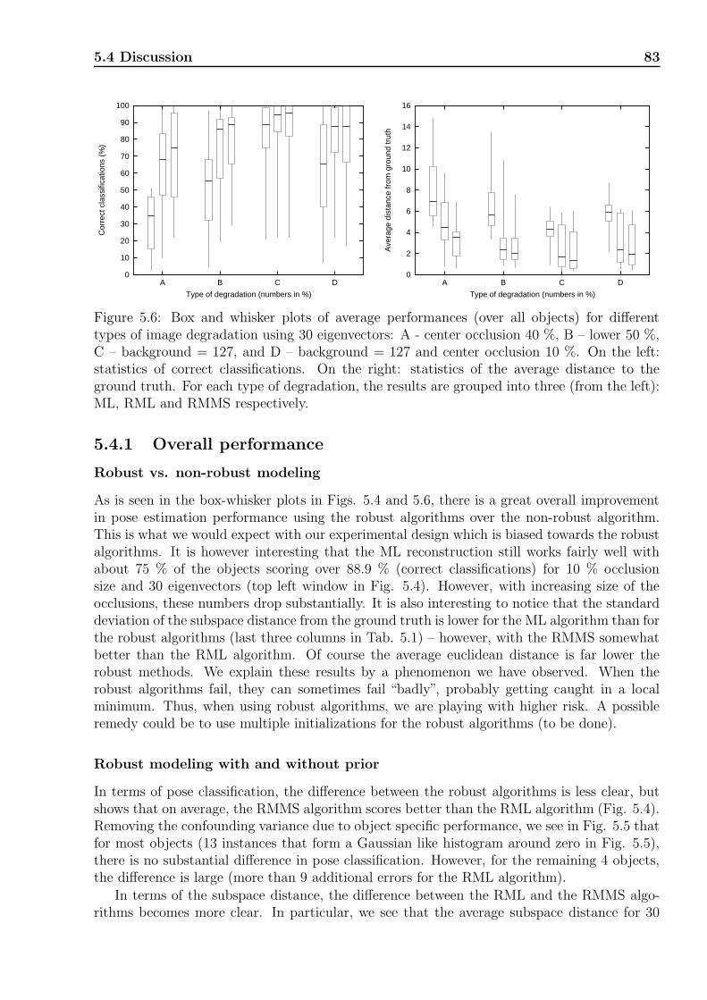
5.4 Discussion 83
0
10
20
30
40
50
60
70
80
90
100
DCBA
Cor
rect
cla
ssifi
catio
ns (
%)
Type of degradation (numbers in %)
0
2
4
6
8
10
12
14
16
DCBA
Ave
rage
dis
tanc
e fr
om g
roun
d tr
uth
Type of degradation (numbers in %)
Figure 5.6: Box and whisker plots of average performances (over all objects) for differenttypes of image degradation using 30 eigenvectors: A - center occlusion 40 %, B – lower 50 %,C – background = 127, and D – background = 127 and center occlusion 10 %. On the left:statistics of correct classifications. On the right: statistics of the average distance to theground truth. For each type of degradation, the results are grouped into three (from the left):ML, RML and RMMS respectively.
5.4.1 Overall performance
Robust vs. non-robust modeling
As is seen in the box-whisker plots in Figs. 5.4 and 5.6, there is a great overall improvementin pose estimation performance using the robust algorithms over the non-robust algorithm.This is what we would expect with our experimental design which is biased towards the robustalgorithms. It is however interesting that the ML reconstruction still works fairly well withabout 75 % of the objects scoring over 88.9 % (correct classifications) for 10 % occlusionsize and 30 eigenvectors (top left window in Fig. 5.4). However, with increasing size of theocclusions, these numbers drop substantially. It is also interesting to notice that the standarddeviation of the subspace distance from the ground truth is lower for the ML algorithm than forthe robust algorithms (last three columns in Tab. 5.1) – however, with the RMMS somewhatbetter than the RML algorithm. Of course the average euclidean distance is far lower therobust methods. We explain these results by a phenomenon we have observed. When therobust algorithms fail, they can sometimes fail “badly”, probably getting caught in a localminimum. Thus, when using robust algorithms, we are playing with higher risk. A possibleremedy could be to use multiple initializations for the robust algorithms (to be done).
Robust modeling with and without prior
In terms of pose classification, the difference between the robust algorithms is less clear, butshows that on average, the RMMS algorithm scores better than the RML algorithm (Fig. 5.4).Removing the confounding variance due to object specific performance, we see in Fig. 5.5 thatfor most objects (13 instances that form a Gaussian like histogram around zero in Fig. 5.5),there is no substantial difference in pose classification. However, for the remaining 4 objects,the difference is large (more than 9 additional errors for the RML algorithm).
In terms of the subspace distance, the difference between the RML and the RMMS algo-rithms becomes more clear. In particular, we see that the average subspace distance for 30

84 Experiments
eigenvectors and 40 % occlusion size (top right window in Fig. 5.4) is quite substantial. InFig. 5.5, we can even see that this distance is systematically lower for the RMMS algorithmthan for the RML algorithm. Since the prior information in the RMMS model acts as a regu-larization term, this was indeed expected. To what degree this distance is important however,depends on the particular application at hand.
Meaning of subspace distance
Since the RMMS model shows better results concerning the subspace distance than the RMLmodel, one might ask what this distance actually means. Recall that the learning data waswhitened, so that the subspace variance of these samples is one. The average distance to thenearest neighbor was measured to about 3.7 for all objects. In this particular experiment wherewe searched to correctly classify poses, this distance seems to be less important as illustratedin for example the rows 4, 5 and 6 (objects 11, 12 and 20) of Tab. 5.2. Here, we see thatfor certain objects a subspace distance of 10 or larger does not necessarily lead to a wrongpose classification (based on the nearest neighbor classification). However, as these examplesalso show, it is difficult to make any general conclusions about how large this distance shouldbe. For object 20 (second to last row), the RML algorithm leads to a wrong pose estimationat a subspace distance of 4.56, whereas just above we see that even with a subspace distanceof 8.06 and 10.13 (objects 12 and 11 respectively) the pose is correctly estimated. Generallyspeaking however, it is clear that the reconstructed objects are visually closer to the originalwhen this distance is small.
5.4.2 Modeling issues
Importance of model accuracy
We shall shortly present the argument that there is no simple relationship between the vari-ance described by the model and the results we have obtained. There is however, a generalimprovement in the classification performance with a more accurate model in the form of anincreasing number of eigenvectors as seen in the left windows4 of Fig. 5.4. Other experimentswe have performed with fewer eigenvectors also support this. We further believe that anothermore subtle relationship can be deduced from these results, namely that the RMMS modelprofits more from increased model accuracy than the RML model. This conjecture is sup-ported by the histograms in Fig. 5.5 where we see that the histograms are skewed slightlyto the right (and thus in favor of the RMMS model) for 30 eigenvectors with respect to 15eigenvectors. This relative difference is not unambigously clear from Fig. 5.4. Another reasonwe believe that this supposition is correct is given by the results found for object 15 which arediscussed below. An accurate model therefore seems to be important in order to obtain goodresults with the RMMS model.
Relation between model variance and object performance
One observation from these experiments is the large differences in the performances obtainedfor different objects. Are these differences mainly attributable to the objects themselves orto the fact that we have chosen a fixed number of eigenvectors across which we compare
4Note that we cannot make the same comparison with subspace distances since these are not directlycomparable for 15 and 30 eigenvectors.

5.4 Discussion 85
performances? Instead of fixing the number of eigenvectors, one often fixes a proportion ofexplained variance based on Eq. 3.5, p. 35. However, as we noticed, there is no simplerelation between the performances we have observed and the variance explained by the model.This becomes clear when studying the relation between the results given in Tab. 5.1 and theproportion of variance explained, given in Fig. 5.7. For example, 30 eigenvectors describe96.4 % of the total variance of object 8, but only 88.8 % of the total variance of object 9.However, the performances of object 9 (Tab. 5.1) are largely superior to those of object8. There is thus no simple relationship between object specific variance and the observedperformance (but see also the next paragraph). These differences are more related to thedifficulty of occlusions as discussed below (Sec. 5.4.3).
Appropriateness of subspace modeling
Two small aspects are worth mentioning here. First, given the particular subspace distributionof these image sets (Fig. 3.4, p. 38) it is clear that using a kernel estimator to estimatethe density results in a rather “bumpy” distribution. When using all the object images forlearning – as we have done in this experiment – this estimate is probably sufficient. It ishowever in general a difficult distribution to estimate using a kernel estimate because the truedistribution should be constant along the thread of points. This problem is similar to theproblem of estimating a uniform distribution in one dimension using a kernel estimate whichrequires a high number of kernels to be well estimated.
The second aspect concerns the dimension of the subspace and non-parametric densityestimation. The curse of dimensionality dictates an explosively high number of samples in orderto correctly estimate a high dimensional density. In their article on the mean shift, Comaniciuand Meer [40] argue that the method is only appropriate up to about six dimensions. However,we are actually observing that the subspace modeling adds value even for 30 eigenvectors.Maybe one could say that some subspace estimation is better than none.
5.4.3 Experimental issues and practical concerns
Occlusion difficulty
It is clear that most of the object specific performance differences that we observe in theseexperiments must be attributed to what we call the “occlusion difficulty”, i.e. how muchdoes a particular object suffer from the artificial degradation it has been subjected to. Forexample, consider object 12 or object 20 with respect to object 1 in Tab. 5.2. Whereas it isextremely difficult, even for a human observer, to estimate the correct poses of the degradedimages 12 and 20, this is a fairly simple task for object 1. Even so, it is interesting to notethat there are large differences in performance on these objects (RMMS, Tab. 5.1 and Fig.5.4): whereas the pose of object 12 was correctly estimated for all 72 poses – indeed veryimpressive, this number is only 20 (27.78 %) for object 20. For 30 % occlusions, the number ofcorrect pose classifications for object 20 becomes 67 (93.06 %). It is therefore quite reasonablethat the degradations we have applied to the images – even though identical – lead to quiteheterogeneous results across the objects.
Computational time
The drawback of the RMMS model is that the reconstruction becomes fairly cost intensive. Wehave not made any theoretical analysis of the computational complexity of these algorithms,

86 Experiments
"!#%$'&)("+*
, -./ -0122 345 -/ 026789
: ; < = > ? @ A B :C :: :; :< : = :> :? :@ :A :B ;CCD CEFGCC:D CEFGC?;D CEFGC?<D CEFGC?=D CEFGC?>D CEFGC??D CEFGC?@D CEFGC?AD CEFGC?BHD CEFGC?:D CEFGC@:DI:EFGC@:D ;EFGC@:D <EFGC@:D =EFGC@
JKLM
NPOQ RGSTVUXW)YZR)[
\] ^_` ab cdefg ehicb f ahieb cj
Figure 5.7: Top: percentage of variance explained by 15 and 30 eigenvectors (Eq. 3.5, p. 35)for each of the COIL-20 objects. Bottom: absolute variance that is not explained by 15 and30 eigenvectors.

5.5 Conclusion 87
Occlusion size Object 15 eigenvectors 30 eigenvectorsRML RMMS RML RMMS
10 % 1 1.6 8.9 2.9 248 1.2 9.6 3.3 29
30 % 1 1.3 11 3.6 368 6.8 88 11 344
40 % 1 1.6 12 3.5 378 6.0 109 11 312
Table 5.3: Example of computation times in seconds as experimentally observed for object 1and 8 at pose 0. We see that the computation time depends strongly on the object and theocclusion. Generally, the computation time increases with increasing occlusion size and withan increasing number of eigenvectors used in the model. ML reconstruction is always fast(∼ ms).
nor any convergence analysis. However, it can be seen from Eq. 4.34, p. 69, that the subspacemean shifting (prior term) depends on the number of samples and the subspace dimension.With the modified noise variance matrix due to the robust weights, there is also a dependenceon the observation dimension (data term in Eq. 4.34). Furthermore, the computation dependson the type and severity of degradation of the image. In practice we observed that thereconstruction times varied greatly with the RMMS algorithm. Some examples that wereobtained with our implementation are shown in Tab. 5.3 (code in C++, running on a Linuxoperating system over a 2.4 GHz Pentium 4 with 2GB of memory).
Other models
In these experiments we chose to concentrate on the three models ML, RML and RMMSinstead of evaluating every model that was derived in Ch. 4 (and listed in Tab. 4.1, p. 72).This was done because of practical concerns (too many results can occlude principal trends),but also because we considered that these models would be most interesting to contrast inthis particular experiment. The GMAP and RGMAP models were not considered because wealready knew that the subspace distribution was far from Gaussian. The “Weighted” (non-isotropic) models were not considered because we have not derived the maximum likelihoodestimates of the model parameters (notably the image generating matrix W ) for all thesemodels yet. For the models we have used, we considered that the eigenvectors were sufficientlygood estimates of W since these models are closer to the PPCA model and for this model theeigenvectors asymptotically becomes the maximum likelihood estimate of W .
5.5 Conclusion
We have performed a series of experiments on the COIL-20 database. We conclude from thesethat a general learning approach to object modeling is indeed difficult. This is evident from thehigh variability of results across the different objects of the database. The results do howevershow that on average, the added prior modeling does significantly improve performance. Ingeneral, added modeling does in many cases lead to a more constrained model. However, inour case, because of the general form of this prior distribution, we have quite a versatile model

88 Experiments
that does not seem to be constrained in any particular way with respect to the other modelswe have considered. Several paths for further investigation are open. In particular, we wouldlike to continue investigating the results for the objects 15, 16 and 17 of the database. It wouldalso be interesting to compare these results to the non-isotropic models developed in Ch. 4.
These experiments show that the improved modeling of images as well as the accuratereconstruction of new images under the model is important in order to obtain high recognitionperformances when the images are highly degraded. In the next part of this document, weshall be concerned with the comparison of images of brain perfusion of potential patients withan atlas of normal subjects. These images might potentially contain large zones of abnormalbrain perfusion. As we shall use the residual between the observed image and the reconstructedimage as a measure of abnormality, it is important that the reconstruction task be performedas accurately as possible. The recognition task in this medical setting can be interpreted asthe problem of determining the nearest equivalent normal image to the image under evaluationand corresponds to solving the reconstruction problem.

Part III
Brain Perfusion Atlas: Constructionand Evaluation


Chapter 6
Models and preprocessing: overviewand state of the art
The goal of this work has been the creation of an atlas of brain perfusion as seen in SPECTimages (Ch. 2). We chose to do this using statistical models from the domain of computer vi-sion/pattern recognition (Part II). In this chapter, we start by defining an atlas and explainingthe connection to the problem of pattern recognition. We then review statistical models usedin the analysis of functional brain images. In order to situate these models, it is necessary tounderstand the different clinical or research questions for which answers are sought. Attemptsto answer these questions lead to different experimental designs. An atlas can be consideredto be a special case in experimental design. The notion of experimental design comes fromstatistical hypothesis testing and has an analogue in the formulation of statistical patternrecognition systems. Finally, we review image preprocessing techniques that are necessary inorder to make statistical modeling possible: registration, segmentation and normalization.
6.1 Atlas, definition
What is a probabilistic atlas of brain perfusion? An atlas can best be described by answeringthe following three questions:
1. What does it describe?
2. How does it describe it?
3. For what can it be used?
For example a geographical map is a description of a part of the earth. It describes the spatialdistribution of hills, forests, roads, houses etc. This is done by means of an image using specificsymbols to signify different objects or elements being described. Finally the map can have amultitude of uses, like finding the shortest path between two houses.
Neurologists are interested in atlases of the brain. There exist anatomical and functionalatlases. Anatomical atlases are maps describing the shape, size, spatial extent and relativelocations of different brain structures. Functional atlases uses the same features to describedifferent physiological processes in the brain and how they are related. A functional atlasof the brain contributes to explain how the brain works, a question that has thrilled human

92 Models and preprocessing: overview and state of the art
curiosity for at least a few thousand years1!In our application, we can answer the questions posed in the introduction of this section
as follows: (1) The atlas describes patterns of brain perfusion. By perfusion pattern, weunderstand the level of blood flow (intensity) and the spatial distribution of it in the brain.Measures of these brain perfusion patterns are obtained from SPECT images. (2) The atlasdescribes patterns of brain perfusion by statistically modeling the intensity values observed ateach voxel. (3) The purpose of the atlas is to detect abnormal perfusion patterns in an imageby assigning to each voxel a measure of normality.
We thus arrive at the following definition: A probabilistic atlas of brain perfusion is astatistical model that describes patterns of brain perfusion in a population and allows forinferences about new, unseen patterns relative to this population.
6.2 Overview, construction and modeling
To see how an atlas can be related to a classical pattern recognition problem, let us consider ageneral pattern recognition framework as depicted in Fig. 6.1. Here, we distinguish betweenlearning and classification. In learning, we are concerned with the choice of data representationand/or to extract characteristic features of the data. This is done with the goal of finding anappropriate statistical model that can describe and/or capture salient properties of the data.The statistical model is typically parametric (in order to be compact) and its parameters areestimated from a set of learning patterns. Based on this model a decision rule is defined, whichis then implemented as the classifier itself. New patterns are processed in the same manner asthe learning patterns before they are classified or they may possibly be characterized in somemanner. In our case this process consists of identifying regions of abnormal brain perfusion inSPECT images.
The exact preprocessing steps to be performed might vary slightly. In general, however,registration, segmentation and normalization of the images is necessary, Fig. 6.2. When com-paring brain images, a first step is to align them. This is done using registration algorithms.We describe different problems and possibilities of registration in Sec. 6.4. Second, the ob-served gray values must be made comparable. As we have seen in Ch. 2, the total number ofphotons emitted may vary due to, among other things, variation in the injected dose. Suchvariations lead to global differences in the image intensities and must be compensated. Wedescribe and review the methods of intensity normalization of SPECT images in Sec. 6.6.Finally, only the brain is considered for statistical modeling. This is because the activitydistribution in the surrounding tissues has properties different from those of the brain (Sec.2.6.2). Furthermore, a segmentation is sometimes necessary for the intensity normalization ofthe images. The segmentation of the brain does not represent a major concern, but we pointout the different techniques that have been applied in Sec. 6.5.
6.2.1 Non-probabilistic approaches
The focus of this thesis has been on probabilistic atlases. Another possible, non-probabilisticapproach could easily be deviced based on prototypes and nearest-neighbor comparisons (tem-plate matching). Beside the large memory requirements of this method, we see two inconve-niences. First, in such an approach there is a great risk of sampling prototypes in the tails of
1Actually, what has fascinated the human being is the question of what a human is. The brain seems tobe a good place to look for answers.

6.2 Overview, construction and modeling 93
Choice of features anddata representation
Learning/Model estimation
Classification(Decision)
Measure features
Preprocessing Preprocessing
Learning Classification
Learning patterns Test patterns
Figure 6.1: A general model for statistical pattern recognition. Similar to [110, 58].
Spatial normalization
Database of normal subjects
Intensity normalization
Atlas creation:Estimation of
model parametersComparison
Score image
Image to evaluate
Test image
Atlas
Intensity normalization
Spatial normalization
Learning Classification
Brain segmentation Brain segmentation
Figure 6.2: Overview of atlas creation and image comparison.

94 Models and preprocessing: overview and state of the art
the distribution and therefore sometimes comparing an image to a prototype which is close toabnormal. This makes this approach less robust. The only way of avoiding this problem isto perform some kind of density estimation (parametric or non-parametric), which becomesprohibitive with the large dimension of the observation space due to the curse of dimension-ality. We are therefore in a situation as described in Sec. 3.2.3, p. 31 where the use of adimension reduction techniques (such as PCA) becomes a necessity. Second, we expect anapproach using a dimension reduction technique to generalize better to unseen images thanan approach based on prototypes as it tries to reveal “deeper causes” (structure or patterns)that can explain the observed data.
6.2.2 Pattern recognition and hypothesis-testing
We have seen how the creation and use of an atlas can be considered to be a pattern recognitionproblem. Most methods, however, that have been applied in functional brain studies are basedon statistical hypothesis testing (e.g. whether normal perfusion depends on age, gender etc.).How does an atlas fit into a hypothesis testing framework?. To answer this question and inorder to understand similar statistical models in the literature, it is necessary to clarify theconcept of experimental design (also called study design).
6.2.3 Experimental design
In pattern recognition, we typically are given an application or some kind of system that wewould like to reproduce. This can for example be an automatic system that recognizes a personin a picture. The input and (desired) output of the system is therefore defined. In statistics,however, we anticipate some behavior of a complex system and design an experiment thatcan highlight this behavior. The statistical analysis, of course, depends on this design. Instatistical terms, we say that we make an inference about the behavior.
The goal of the design is to obtain a valid analysis that is as sensitive as possible. Thevalidity of a statistical experiment is assured by randomization and replication. The sensitivitycan be augmented by using analysis of variance models (ANOVA). For further discussion onthese issues, see for example [79]. Let us however clarify some typical aspects on design typesthat helps in the understanding of the neuroscience literature on functional anatomy.
First, we distinguish between studies that are dynamic or not. In dynamic studies (i.e.fMRI studies or cardiologic scintigraphic studies) the temporal order of the images has asignificance and eventual correlations between successive images must be accounted for. Thisis done in fMRI studies by taking the so-called hemodynamic response into account. In studiesthat are not dynamic, the analysis is invariant to the ordering of the images.
Second, we can distinguish between single-subject or multi-subject studies and, in thelatter, whether one or multiple scans are obtained of each subject. In addition to adding inter-scan variability to the model (two-way ANOVA), it can be of interest to model inter-subjectvariability in multi-subject studies (three-way ANOVA) [225]2.
Third, in order to determine the necessary sample size, one distinguishes between twoclasses of inference: inference about “typical” characteristics or about “average” characteristicsof a population. This leads to the notions of fixed - or random-effect models respectively[225, 65]. The former makes an inference about a specific sample (e.g. 5 out of 6 farmersowned a tractor - it is typical that a farmer owns a tractor), the latter makes an inference
2Inter-scan variability is typically modeled as global intensity differences, see Sec. 6.6.4.
6.3 Related work and statistical models 95
about the population from which the sample has been taken (e.g. farmers in Alsace have,on average, more than 0.86 tractors). Making inferences or statements about the populationfrom which the sample has been drawn, as opposed to the sample itself, is typically whatinterests the pattern recognition practitioner. This notion is linked to the power of a classifierto generalize from a learning set (sample) to the unseen test set (underlying population).
Fourth, in functional brain studies, one typically distinguishes between three types of studydesign [71]: activation studies, parametric studies and factorial designs. In activation studies,images are obtained for one or more subjects under two different conditions (i.e. activation -rest) and the activated regions are determined. Variations of this consists of analyzing severalpairs of tasks conjointly, and then determining commonly activated regions. Activation studieslead to the classical analysis of variance (ANOVA) design, i.e. presence or absence of an effect.Activation studies are most often associated with single-subject, dynamic studies, but are alsoapplied in multi-subject studies. An analogy to our atlas problematic can be made here. Thenormal subjects are considered as a series of baseline images and the image to test is consideredas the activation image. Activations in the test-image would indicate non-normality.
In parametric studies the relationship between a physiological parameter and the degreeof activation is analyzed (e.g. the dependency of regional perfusion in a specific region onthe frequency of aural word presentation). Parametric studies are analysis of covariance (AN-COVA) models. Finally, in factorial designs, several factors are combined and the interactionsbetween these are analyzed. An interaction can for example be a change in a change: a seriesof baseline-activation pairs before and after giving a drug to a group of subjects. These arethree-way or higher ANOVA/ANCOVA models.
6.3 Related work and statistical models
In this section we present a review of different statistical-based approaches for functionalbrain studies. The review is done with particular attention paid to methods that can beinterpreted as an atlas, like multi-subject studies and studies with none or one replication foreach subject. This includes studies of normal perfusion (atlas description), implicit atlases(activation studies where a single subject is compared with a database) and explicit atlasesas defined in Sec. 6.1. Some related FDG-PET studies of similar design type have also beenincluded. Furthermore, since this work has focused on multivariate methods, we have alsoincluded multivariate activation studies that have been applied in SPECT. However, we donot present activation studies in general. These represent the large majority of functionalbrain studies (fMRI and PET), and are most often interpreted using voxel-wise univariatemodels. A unified formulation of a large number of ANOVA/ANCOVA and MANOVA typehypothesis tests can be formulated by means of the general linear model (GLM) [199]. TheGLM has been implemented in the statistical parametric mapping framework (SPM) [69]3.Voxel-based, implicit atlases and normal perfusion studies are therefore typically studied usingSPM, whereas explicit atlases are typically based on commercial or proprietary software4.
The methods are organized below according to the features and the modeling approachthat are used. As features, we have (1) the voxel values (voxel-based approaches), (2) the mean
3SPM is a software written in MATLABTM for the statistical analysis of functional brain studies. It isfreely available and a large number of “toolboxes” exist for the analysis with other methods.
4In a recent comparison study [129] tailored to SPECT images, SPM was found to be rather unsatisfactoryin comparison with a commercial program BRASS (Nuclear Diagnostics, Sweden), VOI analysis and visualinspection.

96 Models and preprocessing: overview and state of the art
values in a region/volume of interest (ROI/VOI approaches) or (3) the voxel values projectedonto the cortical surface. The modeling approaches are all linear, but we distinguish between(A) univariate models and (B) multivariate models. The univariate models are actually mul-tiple univariate models, one for each feature, e.g. SPM has one linear model for each voxel.These models therefore consider each feature as statistically independent of the other features.“Pure” multivariate models on their side, test all the features as a whole. In order to makelocalized analysis, additional analysis or response characterization is therefore necessary. Wealso consider as multivariate models, approaches where some kind of spatial cross-correlationhas been taken into account.
6.3.1 Other reviews
Whereas this review is more focused on methodological aspects, there exist other reviews inthe literature that cover other aspects. In [127], Van Laere et al. review eleven other studiesof normal perfusion/tracer uptake in SPECT. Since the article reports normal perfusion data,the review is focused on the acquisition parameters in each study (e.g. collimator, number ofcamera heads etc.), as well as the selectivity of the databases representing normal subjects.We have noticed that very few such studies (one and one partially) use MRI co-registration toregister the SPECT images of different subjects (see Sec. 6.4.4). The review reports the majorfindings in the individual studies and indicates whether ROI (VOI) analysis was employed.The statistical hypothesis/models that were used are not reported.
Gardner et al., [76], have made a review of HMPAO-SPECT studies in neuropsychiatricdisorders (schizophrenia and major depression). The review focused on the relating of theoriesconcerning neural substrates in psychiatric disorders with findings in functional brain imaging(using SPECT), i.e. what is the origin of altered radiotracer uptake and distribution in psychi-atric disorders ? Possible methods for functional brain imaging studies are briefly mentioned,but the studies referenced (nine schizophrenia and eleven major depression studies) were notlinked to the methods.
Another review, made by Amen et al. [3], presents different findings in SPECT studiesthat are useful in a clinical setting. For each study they report tracer (ECD, HMPAO, Xe,I123), age distribution, database size, year of study and significant findings. The review isorganized with respect to pathology: normal, brain trauma, dementia, temporal lobe epilepsy.
Finally, let us mention the review in [228, 229] of statistical methods that have been appliedin fMRI and PET studies. In the former, a unified overview of univariate as well as multivariatemethods is presented, whereas the latter only reviews multivariate studies, but in more depth.
6.3.2 Univariate methods
Voxel-based approaches
A list of univariate approaches based on individual modeling of each voxel is shown in Tab.6.1 (all studies were done using SPM). In these approaches, neighboring voxels are consideredto be statistically independent. This is clearly not true in low resolution SPECT images, butcan serve as an approximation. However, because of the high number of statistical tests thatare repeated, one typically has to correct for multiple comparisons, e.g. with a total of 10000brain voxels, a p-level of 0.05 would yield 500 significant voxels under the null hypothesis.In order to reduce this number one uses either the Bonferroni correction [225] (used in for

6.3 Related work and statistical models 97
example [127]) or a posterior correction based on the theory of Gaussian random fields [227]5.These methods of post-correction are implemented in SPM, but does not seem to be employedby all researchers.
In a pattern classification setting, Laliberte et al. have presented a method for classifyingSPECT images as normal or abnormal, based on the comparison with a normal atlas [131].This is done using two features: voxel intensities and voxel displacements (as found by imageregistration, see also section 6.4.5). A univariate test is done at each voxel, one for intensity andone for displacement. Then classification is done based on the number of abnormal voxels.Using cross-validation on a database of 23 subjects with diffuse anomalies and 21 normalsubjects, the best results were obtained by counting abnormal displacement voxels in the graymatter (93% correct classification).
Region-based approaches
Until recently, region-based approaches were the approaches most widely adopted for quantita-tive SPECT studies. With region-based approaches we understand methods where the imagesare segmented into volumes/regions of interest (VOI/ROI) and further analysis is done basedon the mean value of such VOIs. The advantage of these approaches is the reduced noise dueto averaging. A major disadvantage of these methods is their dependence on the segmentation.An error in the segmentation of a region obviously falsifies the mean flow value of the region.A further problem is linked to the so-called partial volume effect (sample aliasing). Becauseof the low resolution of SPECT images, the voxel values on the border between neighboringregions have “mixed” intensity values. This is particularly annoying if the two regions in ques-tion have highly different intensities. In such cases voxels belonging to the region of high (low)intensity will have values lower (higher) than the mean of the region. In small regions, theseeffects can lead to large errors in the estimated flow value.
In Tab. 6.2, two studies are summarized. Both have used VOI-based and voxel-basedanalysis. Tab. 6.3 summarizes two studies that are only based on VOI analysis. Whereas in[203] and [109] the VOIs where manually defined (on 2D slices), the others have registered theimages with a presegmented template to define the VOIs. In [127], the template partitionsthe image, whereas in the (PET) study of Kang et al. [122], the authors calculate a weightedaverage by multiplying the intensity value of a voxel with the probability of the voxel be-longing to a particular brain structure. This probability is given in an anatomic atlas namedstatistical/probabilistic anatomic map (SPAM) from ICBM6. The method can be viewed as asort of fuzzy partitioning.
Surface-based approaches
Another univariate method, denoted 3D-SSP, is based on a quite different feature [157]. Themethod was first developed for PET, but has later been used with SPECT (ECD [5] and [123I]-iodoamphetamine [102]). The method consists of segmenting the brain surface by non-linearregistration of each image with a presegmented template. In addition to the presegmentatedsurface, vectors that point perpendicular, inward from the surface to the center of the brain,are given. The value of each surface pixel is then set to the maximum value found along this
5The assumption of a Gaussian random field is actually in conflict with the assumption of statisticalindependence between voxels.
6There is no reference to this atlas, which was developed at the McGill university by A. C. Evans et al..The ICBM atlases can be found at http://www.loni.ucla.edu/ICBM/ICBM_Probabilistic.html

98
Models
and
pre
pro
cess
ing:
overv
iew
and
state
ofth
eart
Author Application Design Test Regressors Database Tracer Reg. Norm.
Ebmeier et al.(1998) [60]
dementia and depression inold patients
activation,parametric ANCOVA
confounds: age + occipitalROI. interest: MRI measures+ age of onset
depressed (39),ADa (15), normals(11)
HMPAO affineANCOVAocc. ref.
Inference: Early- and late onset of depression, influence of MRI atrophyFindings: Late onset depression associated with more brain changes than early onset
Lee et al.(2000) [135] TLb epilepsy
activation,atlas
t-test patient, ictal, interictalepilepsy (21),normal (9)
ECD affine n.d.
Inference: LateralizationFindings: (Single) Ictal vs. normal better than ictal vs. interictal and better than subtraction method when low threshold
Migneco et al.(2001) [153]
apathy in AD and personalitydisorders (non-demented)
activationANOVAand con-junction
patient group andneuropsychiatric diagnosis
AD (28), PDc (13) ECD affine whole
Inference: Apathy related to hypoperfusion in > ant. cingulate gyrusFindings: Conjunction analysis showed that hypoperfusion in ant. cing. region was common for both study groups
Chang et al.(2002) [32] TL epilepsy
atlas ofdifferenceimages
t-test patientepilepsy (12),normal (7)
HMPAO affine whole
Inference: Localization of seizure fociFindings: Consistent with visual analysis. Ictal is hyper w/ time of injection (t) < 100s and hypo w/ t > 100s
Stamatakis etal. (2002) [198] head injury
atlas,activation ANCOVA
age, scan time (acute andfollow-up)
head injury(61=22+22+17),normals (32)
HMPAO affine whole
Inference: Abnormality in SPECT and MRIFindings: More abnormality detected with SPECT than MRI
Table 6.1: Voxel-based approaches based on univariate statistical methods. All these studies were performed with SPM.
aAlzheimer’s diseasebTemporal LobecPersonality disorder

6.3
Rela
ted
work
and
statistic
alm
odels
99
Author Application Design Test Regressors Database Tracer Reg. Norm. Segm.
Imran et al.(1998) [109]
normal tracer uptakeand validation of AIRa
activation(comparisonto existingatlas)
t-test, brain overlap(co-registration w/X-ray CT as reference)
none normal (30) HMPAO affine whole manual, 2D
Inference: Registration algorithm (human brain atlas vs. AIR)Findings: Max. anatomical variability 4.7mm. differences in rCBF as compared to HBA (which is based on another sample)
Van Laere et al.(2001) [127]
normal tracerdistribution
parametric ANCOVAage, gender,handedness
normal (89) ECD piecewise affine wholepresegmentedtemplate
Inference: Variability, asymmetry, age, genderFindings: Decline w/ age in ant. cingulate gyrus, bilateral basal ganglia, l. prefrontal, l. lat. frontal and l. sup. temporal and insular cortexIncrease in asymmetry w/ age (frontal and temporal neocortex). R. par. high in women, cer. and l. ant. temp. and orbitofrontal high in men
Table 6.2: Approaches using univariate statistical models based on voxels as well as volumes of interest (VOI).
Author Application Design Test Regressors Database Tracer Reg. Norm. Segm.
Tanaka et al.(2000) [203] normal patterns parametric ANCOVA,
t-testage, gender normal (48) ECD proprietary, SPECT
whole,cerebellum
manual, 2D
Inference: Variability, asymmetry, age, gender, >hemispheresFindings: Different results depending on normalization. rCBF decline w/ age in anter. + post. cingulate cortex,sup. prefrontal and parietal cortex, striatum + hippocampus
Kang et al.(2001) [122] TLb epilepsy activation
pairedt-test
lateralizationepilepsy (18),normal (22)
FDG affine whole SPAMc
Inference: Asymmetry in TLFindings: Symmetric VOIs in controls (except inf. temp. gy.), correct lateralization in 14/18, visual inspection consistent in 17/18
Table 6.3: VOI-based approaches using univariate statistical models.
aAutomated Image Registration, algorithm and software for registration from R. Woods [223]bTemporal LobecStatistical/probabilistic anatomic map, International Consortium of Brain Mapping (ICBM)

100 Models and preprocessing: overview and state of the art
inward pointing vector, searching to a depth of 13.5mm (6 pixels). The method is thus basedon a geometric dimension reduction. The surface is then visualized with lateral, superior andmedial views. The authors have used this data representation to create a univariate atlas,consisting of a mean and a variance for each surface voxel. To compare images with theatlas, a z-score is calculated. The atlas has been used in Alzheimer’s disease [157, 5] and topredict hyperperfusion after carotid endarterectomy (deblocking arteries) [102]. Recently, ina comprehensive comparison study, involving 16 nuclear medicine physicians, the method wasshown to improve the diagnosis in Alzheimer’s disease [100].
6.3.3 Multivariate methods
Multivariate approaches in functional brain studies are most widely used in an exploratoryfashion, i.e. to discover relationships between regions. A large number of such approacheshave been applied in temporal studies (PET and fMRI) where such relationships are basedon the idea that brain function is mediated by a network of connected regions (i.e. functionalintegration, see also Sec. 2.4). In multi-subject brain perfusion studies, there is no similarcognitive interpretation of such spatial relationships. However, spatial correlations of brainperfusion across subjects could have a physiological explanation, e.g. higher relative flow valuesin one region is correlated with higher flow values in another region due to a typical vascularstructure. Further exploration of correlation patterns will require interpreting and analyzingthese as a function of age, gender, handedness, etc. as has been done in studies of normalperfusion [179, 238, 115]. Once identified, spatial correlation patterns can be used either asdiscriminators, i.e. to distinguish (classify) two groups [159, 160, 200], or as descriptors ofnormal perfusion variations in a population [104, 105] (which is also implicitly suggested inthe normal perfusion studies mentioned above).
All the models that have been used in multi-subject SPECT studies are linear and basedon either PCA (SVD), Fischer discriminant analysis or partial least squares (PLS). This is incontrast to fMRI, PET and dynamic scintigraphic studies, where other linear models, such asICA [150, 183] and factor analysis [10], as well as non-linear methods, such as nonlinear-PCA[66], have been employed.
Voxel-based approaches
In Tab. 6.4 a summary of multivariate, voxel-based methods is provided. The first author touse PCA to create a SPECT atlas, was Houston et al. [104]. The model is the same as theML model in Tab. 4.1, but has an interesting twist: the residual is analyzed to detect voxelswith abnormal flow values. We have adopted this idea, so let us explain how this is done. Letus recall the linear model from Ch. 4.17:
y = Wx + µ + ε,
where µ is the database average, W is a matrix of eigenvectors (found by PCA), and ε ∼N (0,Ψ) is Gaussian isotropic noise. The noise matrix Ψ is a diagonal matrix of voxel variances.Each diagonal component d, d = 1 . . .D of this matrix is estimated from the learning baseresiduals as follows:
(Σε)d =
(
1
J − 1−Q∑
j
ejeTj
)d
, (6.1)
7The formulation of the method has been adapted from that of the authors’ to fit our own theoreticalframework.

6.3 Related work and statistical models 101
where j = 1 . . . J are the subject indexes and Q is the number of eigenvectors retained in themodel (number of columns of the matrix W . The residuals ej are obtained from maximumlikelihood (or least-squares) reconstruction of the learning base images as:
ej = yj − yj = yj − µ−Wxj, (6.2)
with x from Eq. 4.8 (first row in Tab. 4.1).The atlas is thus represented by the mean, µ, the matrix of eigenvectors (eigenimages) W ,
and the voxel variance Ψ. To compare an image y with this atlas, a residual image e is firstcalculated, which is then compared, voxel-by-voxel, to the learning base variance as follows:
t = Σ−1/2ε (y − µ−Wx). (6.3)
The resulting image, t, is a score image or significance image where each voxel value expressesa significance in terms of deviation from normal values.
A few remarks are worth to mention. First, this model is actually inconsistent. This isbecause the ML estimate is used to solve the reconstruction problem. This assumes isotrop-ical noise. When constructing the score image, however, non-isotropical noise is considered.Nevertheless, we think this inconsistency is not very important in practice8. Second, it is alsointeresting to notice that the model was developed independently of the models in computervision. Finally, we can see from the distribution of the observation when given the subspacevariable, p(y|x) (given in Eq. 4.4, p. 60), that the score image is nothing else than themarginal probability of this distribution at every voxel:
td =
∫
· · ·∫
p(y|x)dy1 . . .dyd−1dyd+1dyD = p(yd|x).
In [104], this method was used to classify subjects with Alzheimer’s disease, infarcts andnormals. In a later study, Houston et al. used the same method to characterize typical patternsof abnormality in a series of pathologies, see also Tab. 6.4.
In a recent, multi-subject PET study, the authors analyzed the dependence of the eigen-vectors (correlation patterns) on age in a normal population [238]. Interestingly, they founda significant correlation between age and the second principal component. Such a relation isalso probable in SPECT, since univariate methods [203, 127] and multivariate, region-basedmethods [115, 179] have shown a similar dependence on age.
Region-based approaches
In Tab. 6.5 we give a summary of multivariate, region-based methods. The mathematicalformulation is analogous to the one for voxel-based approaches: an image is considered to be arandom vector, the elements being mean, regional flow values. In a multi-subject PET studyMoeller et al. calculated correlation patterns in a population with Parkinson’s disease andin normals [159]. In the normal group, representing a large age-span, a set of patterns wereassociated with aging: a score based on the subspace projection of each subject onto thesepatterns was found to correlate strongly with age. In the literature, it is predicted that Parkin-sons’s disease accelerate ageing. However, the scores of Parkinson’s disease patients revealeda negative correlation with the ageing patterns and so the authors concluded that the diseasedoes not accentuate normal change in metabolism due to aging. The correlation patterns here
8In our experiments, the differences in the ML and WML projections were small.

102
Models
and
pre
pro
cess
ing:
overv
iew
and
state
ofth
eart
Author Application Design Test Regressors Correlation Database Tracer Reg. Norm.
Houston et al.(1994) [104] ADa, infarcts atlas z-score patient PCA,
descriptiveAD (10), infarct (12),normal (53+8)
HMPAO affine cerebellum
Inference: Classification (based on the interpretation of abnormal voxels found in the gray matter)Findings: At optimal decision level: AD 10/10, infarct 11/12, one false-positive
Houston et al.(1998) [105]
normals, divers, diversw/decompressionillness, boxers,schizophrenics and AD
atlas z-score patient PCA,descriptive
normals (50+40),divers (18), DCIb (50),boxers (34),schizophrenics (23),AD (21)
HMPAO affine cerebellum
Inference: Typical patterns in different diseasesFindings: Multiple small lesions are as common as single large lesions for divers w/ DCI, not for AD and schizo.Large lesions in parietal and inf. temp. regions in AD. in par. and occipital regions for divers w/ DCI and boxers. Inferior frontal region in schizophrenia
Zuendorf et al.(2003) [238] normal metabolism parametric
ANCOVA,T2 test insubspace
agePCA,exploratoryw/regressors
normals (74) FDG affine whole
Inference: Normal correlation patterns and dependence on ageFindings: Second PCc is more strongly correlated w/ age than first. PC1: in and adjacent to ventricles and basal cisterns.PC2: high loadings on prefrontal, post. parietal and post. cingulate
Table 6.4: Multivariate, voxel-based approaches.
aAlzheimer’s diseasebDecompression illnesscPrincipal component

6.3 Related work and statistical models 103
were found using the so-called scaled subprofile model (SSM). The model assumes that theobserved rCBFij in subject j and region i is composed of three multiplicative components:subject-specific global flow (GSFj), region-specific flow (group mean profile - GMPi) and asubject- and region-specific component (SRPij) as:
rCBFij = GSFj ×GMPi × (1 + SRPij).
From this equation the logarithm is taken in order to obtain an additive relationship and PCAis performed on the SRP to obtain the correlation pattern. To obtain the SRP the authorsproceed by first calculating approximate values for the GSF (as global blood flow) term andthe GMP (average region flow) term. These approximate values are then corrected for afterreconstruction with the estimated SRP. The SSM/PCA method has been used by the sameresearch group in a series of applications [190, 167, 29] and the reproducibility of the patternshas been assessed in [160].
Another multivariate technique, called partial least squares (PLS) has been employed byLeibovitch et al. [136] to characterize typical hypoperfusion in a group of patients that haveleft hemispatial neglect after stroke (they do not perceive visual stimuli from the right). Thetechnique is quite similar to multivariate linear regression, but does not account for any au-tocorrelation [16]. After removing confounding data (age, gender, education and CT lesionvolume), the flow data is covaried with predictor variables from neuropsychological tests. Inthis particular study, 81 subjects were studied, each passed 4 tests and the image data wasquantified into 152 regions. Let Y be the 152× 81 sample matrix of image data with one col-umn for each subject, and let X be the 4×81 test score matrix, also with one column for eachsubject. Whereas PCA consists of approximating the covariance matrix Y Y T , PLS consistsof approximating the cross-correlation matrix using (sparse) singular value decomposition:
Y XT = USV T .
Here, U is a matrix of saliency images (equiv. to eigenimages), the diagonal matrix S containsthe covariances and V the saliency test scores. They found that the relative influence ofthe first saliency image was 94% with an equivalent contribution from all four testscores.This image was therefore interpreted as the significant multivariate response to the (multiple)predictor variables (test scores). Furthermore, each subject’s image data and test scoreswas projected on the saliency image and the saliency test score, and a scatterplot of theseprojections revealed groupings of stroke patients with and without hemispatial neglect. PLShas been criticized in [229] because the results change with scaling of the predictor variables(meaning care must be taken since there is not necessarily a well defined euclidean distancein predictor space). For fMRI and PET, multilinear models [229] and canonical correlationanalysis [64] has been proposed as alternative methods. These have not, however, been appliedin conjunction with SPECT images.
Other multivariate studies (Tab. 6.5) include that of Jones et al., who performed SVD(PCA) on regional flow data [115]. The regions were determined by determining a polar gridof radial spokes and an external contour on image slices. In [200], Stoeckel et al. took a moreclassical pattern recognition approach to classify patterns using Fischer discriminant analysis.Finally, Pagani et al. performed PCA on regional flow data defined by using a software toolthat is called Computerized Brain Atlas [83].

104
Models
and
pre
pro
cess
ing:
overv
iew
and
state
ofth
eart
Author Application Design Test Regressors Correlation Database Tracer Reg. Norm.
Moeller et al.(1997) [159] PDa
parametric ANCOVA agePCA, exploratory+ discriminativew/regressors
idiopathic PD (37),normals (20)
FDG n.d.b whole
Inference: Dependence of covariance patterns with age in patient groupFindings: Age-metabolism relationship is progressively disrupted in PD. PD is not simply accentuation of normal ageing
Jones et al.(1998) [115]
normalpatterns parametric
ANOVA,MANOVA
age, genderSVD, exploratoryw/regressors
normal (152) HMPAO n.d. n.d.
Inference: Age and gender specific correlationsFindings: No sign. change in whole-brain uptake. regional declines in lat. ventr. Higher uptake in women
Leibovitch etal. (1999) [136]
Hemispatialneglect (afterstroke)
activation,classifica-tion
z-score,subspaceprojec-tion
confounds: CT lesionvolume, age, sex,education. covariates:neuropsychiatric test score
PLS stroke patients (49+32) HMPAO n.d.cerebellum(one hemi-sphere)
Inference: Identification of brain regions with hypoperfusion which can be related to hemispatial neglectFindings: Right temporo-parieto-occipital junction is more important than other, earlier reported findings
Stoeckel et al.(2001) [200] ADc atlas,
classifierGaussianclassifier
none Fisherdiscriminant
AD (29), normals (50) HMPAO affine, whole, top 1%
Inference: ClassificationFindings: 90% correct classification
Pagani et al.(2002) [179]
normalpatterns parametric ANOVA age, gender
PCA, exploratoryw/regressors
normal (50) HMPAO CBAd
13% of voxelswith highest in-tensity
Inference: Age and gender specific correlationsFindings: Higher CBF right. Decrease w/ age (in part. left) - stronger in females. rCBF decrease w/ age in vertex,l. frontotemporal and temporocingulate cortex, rel. rCBF increased
Table 6.5: Multivariate, region-based approaches. Moeller et al. also perform voxel-based PCA in addition to region-based PCA.
aParkinsons’s diseasebno descriptioncAlzheimer’s diseasedComputerized Brain Atlas, a commercialized software of segmented anatomical structures and a non-linear registration algorithm with up to 18 free
parameters [83].

6.4 Registration 105
6.3.4 Image databases
Given the large variability of brain perfusion in a normal population, it is obviously importantto develop reference (or normative) data in order to improve the understanding of normalCBF and thus the diagnosis of abnormal CBF. Several studies mentioned in the last sectionhave addressed this question [109, 127, 203, 179]. However, given the complexity of the dataprocessing and the analysis it is difficult to reproduce such results from paper publications.This is why several groups are constructing databases of images that are available on theInternet. The idea of these databases is to provide images and standardized algorithms forthe processing of images. The two major projects for this are: Neurogenerator9, which is aEuropean project and ICBM10 (International Consortium of Brain Mapping), which is a northAmerican project.
However, neither the ICBM project, nor the Neurogenerator provide SPECT images (theyare biased toward PET, fMRI, MRI, cytoarchitectural data, etc.). A more modest projectthat provides normal SPECT images has been initiated by the Society of Nuclear Medicine(SNM)11. Because of less reliable quantification in SPECT, the comparison of SPECT imagesacross centers is, however, more difficult than for PET/fMRI [126]. As a note, the integrationof neuroscience and informatics has been termed neuroinformatics. A list of databases in thisdomain can be found in the bibliography on Neuroinformatics [169].
6.3.5 Partial conclusion
We have reviewed different statistical methods used for group studies and atlas techniquesbased on SPECT/PET images. In order to better situate these, we structured the reviewbased on the statistical approach (uni-/multivariate) and on the feature that is modeled(voxel/region/other). Notions about experimental design and how an atlas fits into statis-tical hypothesis testing is important for understanding relations and differences between theapproaches. We now turn our attention from the modeling aspects to the preprocessing of theatlas.
6.4 Registration
Registration is the problem of superimposing corresponding anatomical structures from twodifferent images of the brain. For a brain SPECT atlas, the goal is to superimpose all thedatabase images so that the intensities observed at a given voxel can be considered to representbrain perfusion at the same anatomical location. For a complete, in-depth survey on medicalimage registration techniques, we point the reader to [145]. In this section we give an overviewof registration techniques that have been of importance to this work. We describe the principalelements of the different registration scenarios and algorithms that have been implicated.These algorithms compose a toolbox that has been used for devising a complete registrationscheme. This scheme is described in the next chapter.
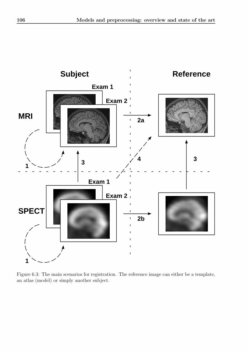
106 Models and preprocessing: overview and state of the art
Subject Reference
MRI
SPECT
Exam 1
Exam 2
Exam 2
Exam 1
1
1
2a
2b
3 34
Figure 6.3: The main scenarios for registration. The reference image can either be a template,an atlas (model) or simply another subject.

6.4 Registration 107
6.4.1 Overview
As seen in the schema Fig. 6.3, we can distinguish four principal registration scenarios: (1)intra-subject, intra-modal, (2) inter-subject, intra-modal, (3) intra-subject, inter-modal, andfinally (4) inter-subject, inter-modal registration. The first scenario occurs when several imagesare obtained for the same subject over time. These must then be registered in order to followthe development of a pathology such as multiple sclerosis [18]. The last scenario can occurwhen we have only one image of a subject (e.g. a SPECT image), in which we would like toautomatically define volumes of interest (VOI). In this case, it is necessary to register the imageacross modalities and subjects. Scenarios 2 and 3 are described in the following paragraphs.
In general, the registration problem can be cast to an energy minimization problem. Forthis, one has to (1) define a similarity measure between images and (2) choose a deformationmodel. Since the resulting target or energy function might be complex, having many localminima, a main problem is to find a good algorithm to optimize the target function. Theprincipal problems in the different scenarios are situated differently. We will now describethese for scenario 2 and 3.
6.4.2 Intra-subject, SPECT-MRI rigid registration
As already mentioned in Sec. 2.3, intra-subject, inter-modal registration has an importantapplication in superimposing functional images (i.e. SPECT, PET) on anatomical images (i.e.MRI, CT). Because the functional images often have a low spatial resolution, it is difficult tolocalize abnormal zones anatomically in the brain. This difficulty is alleviated by bringing thefunctional image into correspondence with an anatomical image of the same subject.
In most applications, the brain is considered to be a rigid structure. One therefore choosesa transformation model that only consists of six free transformation parameters: three fortranslation and three for rotation (assuming there are no deformations caused by the imagingsystem). There are however situations where a 12 parameter affine12 model, or even a de-formable model are more appropriate [18, 45]. The main concern in this type of registrationis the choice of a similarity measure. Since the images have different physical interpretations,one cannot directly compare voxel intensities. Simply minimizing a square error function istherefore excluded. A multitude of different similarity measures have been developed. Thesecan be classified into three different groups: (1) landmark-based [184], (2) surface-based [95]and (3) intensity-based [96]. For the first two groups, it is fairly easy to define a similaritymeasure between landmarks or a surface. However, the problem’s focus has been shifted tothat of the automatic detection of landmarks or the segmentation of surfaces.
For fully automated registration, intensity-based measures seem to yield the best results.The most successful intensity-based measures have been the “Wood” criterion [224] (also vari-ance of intensity ratios), cross-correlation, mutual information and normalized mutual infor-mation.
In a comparative, multi-center retrospective study, the mutual information criterion, to-gether with multiresolution, simplex optimization yielded the best results [222]. This schemehas been implemented by other researchers in our laboratory (Nikou, Musse, Sinapin) andwas accessible for this work. In particular, with this approach, no pre-segmentation of the
9http://www.neurogenerator.org10http://www.loni.ucla.edu/ICBM/index.html11http://brainscans.indd.org/brncncl4.htm12An affine transformation maps parallel lines on parallel lines

108 Models and preprocessing: overview and state of the art
Figure 6.4: Example of a SPECT exam registered with a MRI exam of the same subject usinga rigid transformation model (translation and rotation). The images are superimposed withthe SPECT image displayed in colors (violet for the lowest values, over orange to white forthe highest intensity values) and MRI in gray values “underneath”. The registration is indeed,visually satisfying.
scalp is necessary and the capture range (“distance” of initial displacement, still yielding goodresults) is rather good. The problem of SPECT-MRI registration of the same subject is largelyconsidered to be “solved” since a precision of about a few millimeters is reached and consideredto be sufficient. Visual assessment of the quality of SPECT-MRI registration is neverthelessnecessary. This is best done by superimposing the transformed SPECT image on the MRimage, using a color palette for the SPECT image. An example is shown in Fig. 6.4.
6.4.3 Inter-subject, MRI deformable registration
Whereas for intra-subject, SPECT-MRI registration the main problem is to define a robust,sensible similarity measure, the main problem in inter-subject registration is to define a (valid)deformation model and to solve the related optimization problem. Given the high anatomicalvariability between subjects, an affine transformation model is not sufficient. For example,gyri and sulci are defined by how the cortex is folded, and some of these show high variability(typically those that are developed late in the fetus [214]). Ideally, one would like to have aglobal deformable, parametric model that could span all brain “prototypes” and at the sametime be mathematically tractable (or more precisely: computationally tractable). This isthe case for the cortex, which is inherently a two-dimensional surface. The best method forcomparing the cortex of different brains therefore consist of segmenting the outer cortex andinflating it to a sphere [49, 61]. This method is however not adapted for the whole brain. Asimilar method maps the outer cortex to a sphere and permits the mapping of deeper structuresas well, but necessitates much user intervention [207].
A vast literature on intensity-based methods for deformable matching of brains, witnessesthe complexity of the problem [145, 208]. These range from physical models (e.g. elasticand fluid deformation models) to purely mathematical models (e.g. polynomial-, Fourier- orspline-based deformation models). In our laboratory, an algorithm based on the hierarchicalspline-decomposition of the transformation has been developed [166, 172, 173, 174]. Theprincipal properties of this algorithm shall now be described.

6.4 Registration 109
Figure 6.5: First order B-cubic spline functions in one dimension at two different scales (sup-ports).
As for all deformable registration algorithms, the images are first brought into an initialregistration using an affine transformation model. This affine transformation compensatesfor global differences in position, rotation, shear and size between the two brains. From thisinitial registration, a discrete deformation field is calculated. This field is a parametrized fieldof vectors that define the spatial displacement of each voxel. The parametrization is done bychoosing a representation of the field using basis functions. First order B-cubic splines werechosen as basis functions (see Fig. 6.5). They were chosen (among other reasons) becausethey are well adapted to a multiscale approach (i.e. the B-cubic splines are scaling functionsassociated to wavelet representations). This means the algorithm can start by minimizing thecost function associated with a large scale decomposition of the field, i.e. large spline supportand thus few parameters. The resulting minimum is used to initialize the decomposition ofthe field at a finer scale. Since there is an analytic relation between the field decomposition atdifferent scales, this transition is simple. The algorithm thus calculates a deformation field atfiner and finer resolutions that gradually compensates for anatomic differences. See Fig. 6.6for an illustration and Fig. 6.7 for a synthetic example of this registration.
Whereas the main problem in inter-subject registration is to define an appropriate deforma-tion model, the choice of similarity measure is of course also important. As an intensity-basedcriterion, the sum-of-square-residuals,
Cq(h S,R) =∑
pi∈Ω
(S(h(pi))−R(pi))2, (6.4)
has been the most popular. Here, S designates the source image, R is the reference imageand h is the transformation that transforms S into correspondence with R. The sum iscalculated over the support of the images, Ω. This criterion is not symmetric, that is, thetransformed version of the source images is compared to the reference image13. Because ofsampling errors and limitations of the transformation model, one does not in general obtain theinverse transformation of h when swapping reference and source image. This led the authors
13Actually the roles of reference and source image is inversed in practice since an inverse transformation iscalculated. This is in order to avoid the so-called forward-sampling problem: Because the transformation isnon-linear, the regular source grid is not necessarily transformed to a regular grid. This can lead to holes inthe transformed image.

110 Models and preprocessing: overview and state of the art
scale l
scale l+1
scale l+2
scale transition
minimization
minimization
scale transition
Figure 6.6: Illustration of the multiresolution approach where the deformation field is graduallycalculated at finer and finer resolutions (courtesy of V. Noblet).
in [38] to propose a symmetric criterion instead:
Csym = Cq(h S,R) + Cq(S, h−1 R) =
∑
pi∈Ω
(S(h(pi))− R(pi))2 +
∑
pi∈Ω
(S(pi)− R(h−1(pi)))2.
This has been taken into account in the registration algorithm that we use [173]. Furthermore,the square sum measure in Eq. 6.4 was replaced by a Lp-criterion (p=1.2) (see also Sec. 3.5.2)
CLp(h S,R) =∑
pi∈Ω
|S(h(pi))− R(pi)|p,
which can be considered to be more robust to gross outliers than the square sum [173].Other factors such as interpolation and intensity normalization also influence the regis-
tration. Undersampling of the physical reality leads to aliasing effects which might lead toviolation of the assumptions on the deformation model. Physical and anatomical factors mightlead to inhomogeneities in the images. These again can lead to errors in the cost function (sim-ilarity measure), so that a global minimum of the energy function does not correspond withwell registered images.
Because of the complex structure of the matter let us at last mention that the validationof a registration procedure is extremely difficult [226]. This is because the ground truth is notknown and the definition of what a good registration is depends on the application. Imageregistration has many applications, but only few new methods are taken to clinical practicewhere their impact on diagnostics and treatment can be measured [145]. The animated view(displaying the images in sequential order) of the transformed image and the reference imageis a useful tool since human vision is extremely sensitive to movement.
6.4.4 Methods for inter-subject SPECT registration
The main problem encountered in SPECT-SPECT inter-subject registration, is the reliableestimation of the transformation parameters. This is because of the low structural informa-tion present in SPECT images. Direct registration of SPECT images is most reliable for

6.4 Registration 111
A
B
C
D
E
Figure 6.7: Example of non-linear, hierarchical registration at different resolutions. (A) Ref-erence image. (B) Synthetically deformed image. (C) Registration at the second scale (81 freeparameters). (D) Registration at the third scale (1029 parameters). (E) Registration at thefifth scale (89373 parameters). The algorithm consecutively corrects for deformations of finerdetail (courtesy of V. Noblet).

112 Models and preprocessing: overview and state of the art
low-parametric transformation models (i.e. rigid, affine), which are less accurate in terms ofaligning anatomical structures. Even though such registration has been “validated” for sta-tistical pooling of SPECT images [109], we have found that structural variation still remainssignificant. This could be assessed in the evaluation study in [221], also described in Ch. 8.
Another approach to SPECT-SPECT, inter-subject registration is to co-register SPECTimages with the MRI scans of the same subject. The transformation obtained by MRI-MRI,inter-subject registration can then be applied to the co-registered SPECT images (composingstep 3 and 2a in Fig. 6.3). This has the advantage that one can obtain a precise inter-subject registration using deformable transformation models that are reliably estimated fromhigh-resolution MR images.
At last, let us mention that there also exist approaches where deformable SPECT-SPECTregistration is done directly. In [131] for example, the authors have used a daemons-basedapproach for non-linear registration of SPECT images. The method is described in [111].
6.4.5 Integrating registration into the statistical model: modeling
anatomical variance
In the scheme that we have depicted in Sec. 6.2, we have considered the registration to be aseparate preprocessing step that is independent of the statistical model. This is not the onlyapproach possible. The morphological deformation, which is necessary for the compensationof anatomical differences, contains information about a particular subject. Many neurologicaldisorders are associated with morphological atrophy, which again leads to modifications insuch deformations. An interesting approach is therefore to consider a statistical model thattakes into account both morphological deformations and intensity values.
This has been done in [206, 209], where the transformation fields themselves are modeled.A field is a vectorfield of displacement vectors, defined on the same support as the image.The statistical model is simply a 3-D Gaussian distribution for each displacement vector. Thedistribution is estimated by registering a large number of images onto a reference image. In[131], the displacement vector is used for classification of the brain into a normal or a pathologicclass. Further, statistical modeling of deformation fields is also possible. For example, LeBriquer et al. have explored the possibility of decomposing a group of deformation fieldsusing PCA [24]. Rather than modeling the deformation fields themselves, Machado et al.have instead modeled the variance of the jacobian of the deformation fields [143]. Since thejacobian is a measure of local volumetrical change, large changes may indicate anatomicalabnormality.
6.4.6 Structural approaches to inter-subject comparison
Most approaches in the neuroimaging community are based on so-called coordinate-basedregistration and image comparison. This is in contrast to the neuroscience community wherea structural approach is taken and links are sought between architectural and cognitive models.Another approach to group analysis (atlas or group comparisons) as proposed by Mangin etal. [146] is therefore the so-called structural approach (see also [140]). Here, the idea is totransform the raw image into a structural representation (an approach often used in computervision). For example, in [147] the authors use image segmentation techniques based on apriori information (atlas, learning) and the grey levels of the image in order to delineate gyriand sulci of the cortex. A structural representation is then obtained as a set of features for

6.5 Brain segmentation 113
each sulci (shape, position) and their interrelations. This leads to a graph representation andregistration is performed as graph matching. Comparisons can then be done across graphnodes and features. An approach to SPECT atlasing based on for example VOIs could easilybe devised from this kind of structural registration. With the first results appearing, [147]this kind of approach does indeed seem to be very promising. A strong argument in favor ofthe method, is that it facilitates the integration of neuroscientific knowledge into the analysisas shown for example in [27]. Here, models of the neurogenesis is taken into account and thedevelopment of the cortex is studied. However, as the approach is composed of a large rangeof techniques (image segmentation, pattern recognition, artificial intelligence techniques andothers - which all must be evaluated and implemented) its application remains complex andtherefore difficult.
6.5 Brain segmentation
We understand by segmentation of SPECT images to be the classification of every voxel intodifferent classes with a physical meaning. In our model, we are interested in segmenting thebrain, which is our structure of interest. This is a fairly simple task that can be done by thresh-olding the image. The most widely used approach in the literature, consists of fixing a relativethreshold, such as 40% of the maximum value in the image. This normally separates wellthe scalp and ventricles from the cortex (white and gray matter), which has higher intensityvalues in general. However, there exist other methods such as the one described in [154] wherethe authors have modeled the images using a 3D Markov random field model combined witha density mixture model. We have not considered methods for the segmentation of SPECTimages into finer structures. Nevertheless we can mention that ROI/VOI segmentation ofSPECT images is often done by registering with a template (atlas), see Sec. 6.3.2.
6.6 Intensity normalization of SPECT images: Existing
approaches
The intensity normalization is at the heart of quantitative SPECT imaging14. In order tocompare the activity distribution between subjects or scans, the observed counts must signifyabsolute measures of this activity. Reporting absolute values of rCBF also makes it possibleto compare values across imaging centers. The problem of obtaining quantitative measures inemission tomography is subject to active research15.
Among the different factors leading to count errors, it seems to be important to correctfor scatter events. This can be done by modeling such errors during image reconstruction (us-ing algebraic reconstruction algorithms). Unfortunately, the classical filtered backprojectionalgorithm, which is much faster, is the standard algorithm used in clinical settings, and wasthe only one available for the images used in this work. In this section we review the differentapproaches for SPECT intensity normalization used in the literature. However, there does notexist many comparative studies or studies that assesses a method’s validity. As seen in Ch.8, we found that such normalization had a high impact on the atlas that was created, but wecould not assign validity to the different methods.
14It is more accurate to speak of semi-quantitative SPECT as discussed in [43]. The literature prefers theterm quantitative however.
15See for example http://www.imed.jussieu.fr/

114 Models and preprocessing: overview and state of the art
6.6.1 A controversial topic
Whether intensity normalization based on analysis of the images themselves is possible or not,is a topic of discussion, see [43]. Here, one author argues that the normalization of countvalues to a reference region yields results that are satisfactory. The opponent however, arguesthat such normalization may lead to random error as a cause of variation in any region of thebrain. The alternative method of measuring the arterial input function during the injectionof the tracer is therefore preferred. However, this measure is considered to be unpractical orinvasive and is therefore rarely applied. In our study, such measures were not available so wehad to consider methods for intensity normalization.
Many different strategies for intensity normalization have been proposed in the literature,but no consensus exists on which one is the most appropriate. Authors argue that one way ofnormalizing is better than another because it lowers the total variance (sum of voxel variances)in a set of images. This argument is not justified because we can always use a (non-linear) his-togram transformation technique to obtain a global low variance, whether the transformationtechnique is physically justified or not. If we observe different global counts in two images,this might be caused by true global differences (which we do not want to compensate) anddifferences caused by differences in injected dose, head fraction or scanner sensitivity (whichwe want to compensate for by normalizing). The appropriate normalization technique in agiven situation may therefore depend on the application at hand.
6.6.2 Which transfer function?
Intensity normalization can be separated into the choice of a transfer function and the estima-tion of this function. The transfer function maps the observed intensity values in an image toabsolute values. Fig. 6.8 shows a joint histogram (scatter plot) between two images. The jointhistogram is a probability function on S = I1× I2, where I1 and I2 are the gray value range ofimage one and image two, source and reference image, respectively. This probability functiondescribes the frequency of co-occuring intensity values in the two images and is clearly linear16.Existing methods for SPECT intensity normalization therefore only consider linear transferfunctions of the type:
y = γx+ β, x ∈ I1.
We thus have three possible transfer functions: (1) variable scaling factor γ and b = 0, (2)variable constant b and γ = 0 or (3) variable γ and b. For count images, such as SPECTand PET, a proportional scaling factor, a, is considered to be the most appropriate [68].To see this, consider the global CBF (gCBF) to be the same in the two exams: since theproportion of regional CBF remains the same, a difference in injected dose or a difference inthe fraction of dose being distributed to the brain results in the same proportion between rCBFand gCBF. However, this only remains true when assuming that the uptake depends linearlyon the injected product, which is not true for high perfusion rates (Sec. 2.6.2). This mightexplain why fitting a function with an additive constant on the joint histogram is sometimesclearly better than fitting a function without such a constant (see also Fig. 7.5 in the nextchapter). A transfer function only defined by an additive constant exists in a particular casethat will be described in Sec. 6.6.4.
16In MR images however this is rarely the case as shown in, among others, [18].

6.6 Intensity normalization of SPECT images: Existing approaches 115
Figure 6.8: An example of a joint histogram of two registered SPECT images. The histogramis calculated as described in [18, 17], and takes into account the so-called partial-volume effect.
6.6.3 Estimating the transfer function
We first consider methods that have been used to estimate a single proportional factor fornormalization. This constant is calculated by comparing the mean of a reference region toa specified value that is expected for this region. The problem consists in finding a reliablereference region that exhibits this expected value in all image acquisitions. Probably, thesimplest reference region to choose is the maximum value in the image. The choice of themaximum value has the advantage that among all the values in the image, it is subject to thelowest influence of error for the estimation of γ (this is seen by setting γ = vexpected/vreference
and deriving by vreference). However, the maximum value as reference value leads to highervariance in the normalized images than a reference value based on the mean or median. In[185], the choice of the maximum value as a normalization constant, falsified the result in onecase of epilepsy. It is therefore more widespread to calculate the mean or median in a referenceregion such as the whole brain, the cerebellum or more rarely, the thalamus or the basal ganglia[180]. Due to the same reasons as in Sec. 6.3.2 (partial volume effect in VOIs), the latter twoare probably not ideal because of their small size and their location adjacent to regions of lowactivity (ventricles). Use of the cerebellum as a reference region is also error prone. This isbecause an alteration of the perfusion in one temporal lobe can alter the perfusion temporarilyin the contralateral cerebellum (diaschisis).
For the normalization of SPECT images in Alzheimer’s disease (AD) and frontal lobedementia (FLD), Pagani et al. [179, 180] have proposed to use 13% of the highest intensityvalues as a reference region. The choice of the 13% was based on an analysis of the resultingsize of the region in AD and FLD. The highest values were chosen based on the same reflectionas for the maximum value above.
In [185], the authors compared different normalization methods for comparing ictal andinterictal images in epilepsy. Their conclusion was that one scaling parameter was sufficient.The best results were obtained using a robust criterion (maximizing the number of sign changesin the two images to normalize). Linear regression on the scatterplot yielded similar resultsand taking the additive constant into account did not change the results. The reference forthis study was visual assessment of the estimated regression lines in the scatterplot as well asdiagnostic outcome.
Another method has been proposed in [21] for images of patients with epilepsy. For suchimages, it is characteristic to have regions of very low values or very high values. Boussionet al. therefore propose a strategy to automatically determine a reference region that has

116 Models and preprocessing: overview and state of the art
values in the middle intensity range and that has a homogeneous distribution of values. Thisis done by first calculating the mean and variance of the whole brain and then only keepingvalues in the range mean plus/minus one standard deviation. This is done for both images,and the intersection of the remaining regions is chosen as the reference region. An alternativemethod which is based on region growing is also proposed. These methods seems to work wellfor the relative comparison of two images, but they do not scale naturally to the problem ofquantitative intensity normalization of a complete database of subjects.
6.6.4 Integrating normalization in the statistical model: ANCOVA
As with registration, global intensity differences can also be included in the statistical model.This approach has been proposed for activation studies in the SPM framework [68]. Theapproach has the effect of an additive constant for intensity normalization. This constant isdifferent for each voxel and is estimated conjointly with the other predictor variables of themodel.
In SPM, each voxel is modeled separately, and an example ANCOVA model for scanj = 1, . . . , J under activation k = 1, . . . , K is:
ykj = αk + ξ(gkj − g•) + ε
Here, ykj is the observed value at the voxel under condition k for scan j. The activation ischaracterized by the indicator variable αk, which can take on the values +1 (activation) and−1 (no activation). Differences in global cerebral blood flow (gCBF) are accounted for bythe additive normalization constant, ξ, and the difference between gCBF in scan kj and theaverage gCBF in all scans, g•. The noise is considered Gaussian: ε ∼ N (0, σ2). The parametersof the model, αk and ξ, are estimated using least squares estimation (linear regression). Inthis model the distribution of the residual follows an F -distribution and a hypothesis testbased on the measured residual (“extra-sum-of-squares”), with (H1) and without (H0) thecondition factor αk, decides whether a voxel was activated or not. Differently formulated: theextra-sum-of-squares is a measure of how well the αk explain the data.
The alternative to an additive normalization constant, proportional scaling before statis-tical analysis, leads to the model:
γkjykj = γkjαk + γkjε
Here, the noise variance has changed to γ2kjσ
2. The resulting noise is therefore dependenton the scan, with the consequence that the residual does no longer follow an F -distribution.The ANCOVA model is therefore a more rigorous approach than proportional scaling. Theassumption of the ANCOVA model, however, is that the global CBF changes in an additivemanner with changes in injected dose (parallel lines assumption, see Fig. 6.9). This is lessappropriate for SPECT images as we have discussed in Sec. 6.6.2. One could also critizisethat ξ is estimated using linear regression: the global activity, gj, is also measured with errors,not only the rCBF at voxel d. This error is not accounted for in least squares regression (seealso Sec. 7.5). In a later publication, the same authors suggest using proportional scaling forSPECT studies [1].
6.7 Conclusion
In this chapter we started out by defining what we understand by a probabilistic atlas of brainperfusion. An overview of the atlas creation process was given. We then proceeded by review-

6.7 Conclusion 117
gCBF
rCB
F
ξd
g•
1
Figure 6.9: Relationship between regional CBF (rCBF) and global CBF (gCBF) at voxel d,modeled in a ANCOVA type analysis of an activation study where ’+’ signifies activation and’o’ rest. The average global flow over all scans and conditions is g·, the slope is given by ξ. Theαq are the condition dependent flow levels after correction of differences in the global flow. Inan (implicit) atlas study, only baseline images would determine the slope ξ.
ing different statistical methods that are related to this work. This review is complicated bythe large spectrum of applications and methods coming from different domains of research.We have discovered an equivalent method to the appearance-based methods known from com-puter vision but that originated in the nuclear medicine community [104, 105]. The model canbe compared to the ML-model of Ch. 4 and introduces a clever way of comparing an imageto the atlas in order to obtain localized detections. The method is based on analysing theresidual between the reconstructed and the observed images. We embrace this method anduse it to compare images to the atlas.
Our bibliographic review further reveals that the existing atlasing methods all use affineor piecewise affine registration schemes, mostly directly registering the SPECT images fromdifferent subjects. We propose to use a multi-step procedure, passing by inter-subject, de-formable MR registration as is described in the next chapter. We have not reviewed methodsfor image registration (which is a vast domain), but we have described the principal difficultiesrelated to registration and we have given the principal characteristics of the algorithms thatwe have used.
Methods for intensity normalization on the other hand have been thoroughly discussedand reviewed. The discussion show that it is not clear which method is in general preferable.However, after a good registration of two images, the joint histogram (which actually codesthe relation of the relation between many reference regions/voxels) seems to be quite linear innature. This speaks in favour of a linear transformation function easily calculated from thishistogram and is therefore our technique of choice.
The approaches we suggest in the next chapter (Ch. 7) will all be evaluated and comparedto existing methods in Ch. 8.

118 Models and preprocessing: overview and state of the art
Chapter 7
Atlas creation, our approach
In the last chapter, we defined what we understand by an atlas, we reviewed related approachesin the literature, and we reviewed techniques for registration, segmentation and intensitynormalization of brain SPECT images. In this chapter we describe the material and methodsthat we have used and developed. We start by describing the database of normal subjectsthat is represented by the atlas. We also describe the patient image database which wasprocessed in the same manner as the normal images. We then detail a registration schemefor deformable, inter-subject SPECT registration, brain segmentation, intensity normalizationand the statistical models considered. The global work/data flow is depicted in Fig. 6.2. Thevalidation of each individual processing step is rather difficult, but the complete processingchain can be evaluated as is done in the next chapter. We finish this chapter with the resultsof the learning process (atlas creation) and a note concerning implementation issues.
7.1 Database of normal subjects
The database of 34 normal subjects was acquired at the nuclear medicine facility attachedto the institute (Institut Physique Biologique, UMR 7004, Strasbourg), 20 between april anddecember 2001, and another 14 until january 2004. These were volunteers without anatomicalatrophies as seen in the MRI scans. Other exclusion criteria included history of neurological,psychiatric and audio/visual disorders. The project was approved by the ethical committee atthe University of Strasbourg and a written consent was obtained from each subject after beinginformed about possible risks. An MRI scan and two SPECT scans were obtained from eachsubject. The MRI scans were T1-weighted, GE3D sequences with voxel-size of 1mm obtainedon a 2T Bruker scanning device. The SPECT scans were obtained using a Elsinct Helixdouble-headed camera with parallel collimator and filtered back-projection for reconstruction.The full width at half maximum (FWHM) was about 8mm. All 34 images were obtained usinga parallel collimator. In the research protocol, the use of a fan-beam collimator was envisaged,but had to be renounced to due to technical problems. The subjects, 12 men and 22 women,formed two age groups of 26.7± 6.1 and 46.9± 4.3 years (mean and standard deviation).
7.2 Database of patients
At the institute we have access to a database of images of 154 patients with epilepsy. Thesecome from the nuclear medicine service located at the institute. The exams were made withthe same gamma camera as for the database of normal subjects, but most MR images are

120 Atlas creation, our approach
Resampling
Subject to register: SPECT exam
Rigid inter-modal registration
Database reference image ICBM brain template
Affine intra-modal inter-subjectregistration
Deformable intra-modal inter-subjectregistration
Rigid intra-modal inter-subjectregistration
Subject to register:MRI exam
Deformation field filtering
Apply spatial transformation
using interpolation
SPECT
Transformed SPECT in reference system
+ + +
MRI
Atlas
Downsampling
Resolution change
: SPECT image : MR image : Dense transformation field
1
2
3 4 5
6
7
8
9
Figure 7.1: Overview of the registration scheme.
of 2mm resolution. Some of these images show morphological anomalies in the MRI scansand some MR images have slightly different contrasts than those obtained for the normaldatabase. These images have been analyzed by other researchers at the institute using theSISCOM technique described in a later chapter. Six images have been analyzed using theatlas. These results will be described in Ch. 9.
7.3 Spatial normalization: registration
To bring all the database images into a common reference space, we have developed a registra-tion scheme that takes advantage of precise MRI, inter-subject registration as described in Sec.6.4.3. The scheme is depicted in Fig. 7.1 and will be further detailed in the following. Thisscheme is, of course, only applicable in the case where both MRI and SPECT exams have beenmade of the subjects. A particularity of the scheme is the combination of all transformationsinto one single transformation which is then applied to the original image. This limits errorsintroduced by repeated interpolation of the original image. Furthermore, a filtering of thedeformation field obtained by MR, inter-subject registration has been introduced. This stepis further explained in Sec. 7.3.3. As to interpolation, SPECT images were interpolated usingtrilinear interpolation, and MR images using B-cubic spline interpolation [204]. We now de-scribe the choice of reference space before we describe how the combination of transformationswas applied to the SPECT images.

7.3 Spatial normalization: registration 121
7.3.1 Choice of reference image and reference space
As our goal is to bring all images into one spatial reference space, the choice of this space meritssome thought. A major consideration is the visualization of volumetric data. Visualization of3D brain images on a 2D screen is best done by aligning the sagittal plane of the brain withone of the display axis. This way the symmetrical properties of the two brain hemispheres arehighlighted in the coronal and axial views (see also Fig. 2.2). This aids the interpretation ofthe images significantly. The ambiguity in the remaining two axis was settled by Talairachand Tournoux who proposed the definition of a line in the sagittal plane going through theanterior commissure (AC) and posterior commissure (PC), two well defined and relativelystable locations in the brain across a larger population [202]. This line is oriented with theintersection of the axial and sagittal planes. Furthermore, Talairach and Tournoux presenteda “standard“ brain of a 66 year old women (on paper). A cartesian coordinate system withthe origin being defined at the AC point has been superimposed on this brain. This atlas hasbecome a de facto standard reference space in the neuroscience literature, denoted Talairachspace. Global spatial normalization into Talairach space consists of transforming a brain bychanging its position, its orientation and size so that it conforms to the Talairach brain [132].This standard space thus permits different imaging centers to exchange coordinates of differentstructures in the brain (e.g. answering questions of the type “where in the brain” as opposedto “where in this brain”).
Global spatial normalization is today typically done by registration with a (digital) brainimage already aligned in the Talairach space using a 9 (or 12) parameter affine transformationmodel [132]. For this, we have used the ICBM brain template1 which is an average of 452 brainsof normal subjects that have been registered into Talairach space. The template is shown inFig 7.2. Another average brain that is widely used as a reference brain is the average brainof the Montreal Neurological Institute (MNI), McGill University, Canada, which has beencreated from 152 brains2. Both these average brains are somewhat larger than the originalTalairach brain (because of inaccuracies in the registration). The latter average template istherefore sometimes referred to as MNI-space3.
Even though we do not report coordinates of our findings in this work, we appreciate thealignment with the ICBM brain atlas for its visual properties. However, because of the lack ofsharpness of the averaged image, we have not used this template directly as a reference imagefor deformable registration. Several studies suggest that a site-specific reference (or averagereference) image is preferable to an image obtained with another imaging device [81, 85].This might be particulary true for high precision deformable registration which is less robustto differences in contrast and acquisition errors than low-parametric registration. We havetherefore used as reference an (MR) image that was issued from the same imaging device asthose of the database. However, an image outside of the database was chosen to avoid biasedpreprocessing. We chose to use this reference in its original position to avoid interpolationerrors. This explains why we have two reference images in the scheme in Fig 7.1 (“Databasereference image” and “ICBM brain template”). The database reference image is registeredwith the ICBM brain template using a rigid deformation model (rotation and translation) anda sum-of-square residuals cost function. A rigid transformation was prefered over an affinetransformation because the affine would have enlarged the images to that of the average brain;
1From http://www.loni.ucla.edu/ICBM/ICBM_452T1.html2This is the template brain of SPM.3For a discussion on the differences and conversions between Talairach space and MNI space, see http:
//www.mrc-cbu.cam.ac.uk/Imaging/Common/mnispace.shtml

122 Atlas creation, our approach
Figure 7.2: The ICBM 452 T1 brain template is an average brain of normal subjects. Allsubjects were registered using a fifth-order polynomial transformation model. The referencespace defined by this (anatomical) atlas has been referred to as MNI-space, stereotactic spaceor Talairach space.
“our” coordinates are therefore not exactly MNI/ICBM-space. We shall nevertheless refer tothis space as ICBM space.
7.3.2 Registration scheme
Since the algorithms we have used were described in Sec. 6.4, we only summarize the differentregistration steps. See Fig. 7.1 for an overview of the complete registration scheme. We startby resampling the SPECT images to 4mm isotropic resolution (step 1). We then register eachsubject’s SPECT image with the same subject’s MR image (step 2). This is performed asdescribed in Sec. 6.4.2 (rigid transformation and mutual information). Inter-subject, MRIregistration was then performed as described in Sec. 6.4.3 with the database reference imageas the reference (steps 3, 4 and 5). For images of 1mm resolution (2563 voxels), we useddeformable matching with the finest resolution scale level 6 (which corresponds to a splinesupport of 23 voxels, 750 141 parameters). For patient images, that were of 2mm resolution(1283 voxels), we used deformable matching with the finest resolution scale level 5 (also splinesupport of 23 voxels, but 89 373 parameters). After each registration, the transformation andresampled images were stored to disk. All registrations were assessed by visually inspectingsuperimposed views (for SPECT-MRI registration), side-by-side and animated views (for MRI-MRI registration).
7.3.3 Application of transformations to SPECT images: combina-tion and downsampling of deformation fields
In order to avoid accumulation of interpolation errors, the transformations were combined intoone global transformation (step 7 in Fig. 7.1) that took the SPECT images directly from theiroriginal position (in original resolution) to the (subsampled) ICBM reference space (step 9).Care was taken to properly take the different transformations across resolution changes (step8). For the cross-validation study described in the next chapter, this reference space was a
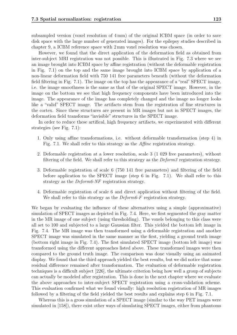
7.3 Spatial normalization: registration 123
subsampled version (voxel resolution of 4mm) of the original ICBM space (in order to savedisk space with the large number of generated images). For the epilepsy studies described inchapter 9, a ICBM reference space with 2mm voxel resolution was chosen.
However, we found that the direct application of the deformation field as obtained frominter-subject MRI registration was not possible. This is illustrated in Fig. 7.3 where we seean image brought into ICBM space by affine registration (without the deformable registrationin Fig. 7.1) on the top and the same image brought into ICBM space by application of anon-linear deformation field with 750 141 free parameters beneath (without the deformationfield filtering in Fig. 7.1). The image on the top has the appearance of a “real” SPECT image,i.e. the image smoothness is the same as that of the original SPECT image. However, in theimage on the bottom we see that high frequency components have been introduced into theimage. The appearance of the image has completely changed and the image no longer lookslike a “valid” SPECT image. The artifacts stem from the registration of fine structures inthe cortex. Since these structures are present in MR images but not in SPECT images, thedeformation field transforms “invisible” structures in the SPECT image.
In order to reduce these artifical, high frequency artifacts, we experimented with differentstrategies (see Fig. 7.1):
1. Only using affine transformations, i.e. without deformable transformation (step 4) inFig. 7.1. We shall refer to this strategy as the Affine registration strategy.
2. Deformable registration at a lower resolution, scale 3 (1 029 free parameters), withoutfiltering of the field. We shall refer to this strategy as the Deform3 registration strategy.
3. Deformable registration of scale 6 (750 141 free parameters) and filtering of the fieldbefore application to the SPECT image (step 6 in Fig. 7.1). We shall refer to thisstrategy as the Deform6-NF registration strategy.
4. Deformable registration of scale 6 and direct application without filtering of the field.We shall refer to this strategy as the Deform6-F registration strategy.
We began by evaluating the influence of these alternatives using a simple (approximative)simulation of SPECT images as depicted in Fig. 7.4. Here, we first segmented the gray matterin the MR image of one subject (using thresholding). The voxels belonging to this class wereall set to 100 and subjected to a large Gaussian filter. This yielded the bottom left image inFig. 7.4. The MR image was then transformed using a deformable registration and anotherSPECT image was simulated in the same manner as the first, yielding a ground truth image(bottom right image in Fig. 7.4). The first simulated SPECT image (bottom left image) wastransformed using the different approaches listed above. These transformed images were thencompared to the ground truth image. The comparison was done visually using an animateddisplay. We found that the third approach yielded the best results, but we did notice that someresidual difference remained after transformation. The evaluation of deformable registrationtechniques is a difficult subject [226], the ultimate criterion being how well a group of subjectscan actually be modeled after registration. This is done in the next chapter where we evaluatethe above approaches to inter-subject SPECT registration using a cross-validation scheme.This evaluation confirmed what we found visually: high resolution registration of MR imagesfollowed by a filtering of the field yielded the best results and explains step 6 in Fig. 7.1.
Whereas this is a gross simulation of a SPECT image (similar to the way PET images weresimulated in [158]), there exist other ways of simulating SPECT images, either from phantoms

124 Atlas creation, our approach
Figure 7.3: SPECT images in ICBM space. The top image was transformed using an affineregistration (without the deformable registration in Fig. 7.1), the image on the bottom usinga deformable transformation (without filtering in Fig. 7.1). The deformable registration iscalculated from high-resolution MR images and the direct application of the resulting transfor-mation introduces artificial, high frequency components into the image. These result from thematching of structures of finer resolution than the SPECT image. These images were trans-formed to 1mm resolution for visualization (2563 voxel images), but the same effect persistedat lower resolutions as well.

7.4 SPECT brain segmentation 125
transformation
High resolution MR images
Low resolution, diffuse, simulated SPECT images
Transformation ?
Non-linear spatial
Spatial
Lowpassfilter
Lowpassfilter
Ground truth
Registration strategy
Figure 7.4: Images similar to SPECT images were created by low-pass filtering the gray matterof a high-resolution MRI image. This way we could obtain a ground-truth transformed SPECTimage from the transformed MR image (bottom right image) to which we could comparedifferently transformed SPECT images (transforming the bottom left image). See the text fora description of the different registration schemes that were compared.
[130, 128] or from MR images [84]. This simplified simulation sufficed however to get an ideaof the influence of the transformation on the SPECT images.
7.4 SPECT brain segmentation
Only the brain is considered for statistical analysis and for intensity normalization. Thisnecessitates the determination of a brain mask. For this we use Otsu-thresholding [178] todivide the image histogram into three classes (corresponding to background, brain and scalp).Otsu thresholding is a histogram thresholding technique similar to k-means clustering. Thegray value distribution of each class is modeled as a Gaussian whose parameters are found bymaximizing the inter-class to intra-class variance. The thresholds are then selected so thatthe Bayes risk is minimized. The highest threshold determined the brain mask (because whiteand gray matter have the highest signal in SPECT). Otsu-thresholding is not always reliablefor SPECT images as it sometimes leads to an overestimation of the brain. In these cases amanual threshold was set.
Typically there remain some “holes” in the brain mask that correspond to the ventricles.These need to be “filled”. This is done by using connected component labeling on the holesand the exterior of the brain (inverse of the brain mask). Clusters of voxels not connectedto the exterior are then added to the brain mask. The connected component labeling isdone successively in the coronal-plane, the axial-plane and finally in the sagittal-plane. Thisapproach was chosen because the holes were too large to be filled with morphological closing.
126 Atlas creation, our approach
The resulting brain mask is sometimes slightly larger than the brain (visual assessment),leading to the modeling of voxels that do not belong to the brain. When analyzing imageswith the atlas we thus expect to have some false alarms on the border of the brain.
7.5 Intensity normalization by total least squares
As mentioned in the discussion on intensity normalization techniques (Sec. 6.6), the evaluationstudy by Perault et al. [185] judged that a two-parameter regression function (scaling plusconstant) was not necessary (scaling was sufficient). However, the fit to the scatterplot isbetter when adding this constant to the model (Fig. 7.5). They argue that a more complexmodel might be more error prone. Still, we propose to use a two-parameter function because,(1) the fit is better, (2) when the images are in good registration, the joint histogram will bequite linear and (3) we use a robust total least squares regression to estimate the functionparameters. In [185] the histogram is linearly fitted using standard least squares. This meansthe x-values are considered to be perfectly measured - without error. Here, x are the intensityvalues in the reference image and y the corresponding values in the source image. If weassume the noise to be the same in both images, a more natural choice is to minimize the sumof square errors orthogonal to the regression line rather than those parallel to the y-axis. Thisis explained in Fig. 7.6. and leads to total-least-squares regression [51]. Total least squares issimply done by calculating the largest eigenvector on the joint histogram. Examples of fittedhistograms are shown in Fig. 7.5.
7.6 Statistical models considered
The statistical models that have been considered in this work are based on the linear modelin Eq. 4.1 and have been summarized in Tab. 4.1, Sec 4.7. These were all implemented andevaluated using the evaluation scheme described in the next chapter. However, their practicaldifferences being small, we only present the results of three representative models in order tobe more conclusive.
Let us recall the linear model Eq. 4.1 from Ch. 4:
y = Wx + µ + ε.
The three models, for which we present results, can then be summarized as follows:
• A univariate Gaussian model - “local”model - which is obtained by setting W = 0. Thenoise is given by ε ∼ N (0,Σε) with Σε being diagonal.
• A multivariate Gaussian model - “global”model - which is the WML model (second rowof Tab. 4.1). The noise is the same as for the local model and the subspace variable isconsidered to be uniformly distributed in the subspace. This model is equivalent to theML model (first row of Tab. 4.1), also proposed by Houston et al. [104] and presentedin Sec. 6.3.3.
• A multivariate robust, non-Gaussian model -“robust global”model - which is the originalRMMS model presented in Ch. 4 (second to last row of Tab. 4.1). The noise is no longerGaussian and the subspace variable is estimated from the training samples using a kerneldensity estimator.

7.6 Statistical models considered 127
y = γx + β y = γx
TLS TLS
y = γx + β
LS
Figure 7.5: Top: Fitted transfer functions using total least squares. The function on theleft has two parameters, scaling and a constant, the one on the right, only scaling. Thetwo-parameter fit is visually more pleasing than the one-parameter fit. Bottom: Fitted two-parameter transfer function using standard linear regression. The slope is clearly too low andthe constant term too high.

128 Atlas creation, our approach
−6 −3 0 3 6−6
−3
0
3
6
x
y
•
•• •••
•
•
•
••
−6 −3 0 3 6−6
−3
0
3
6
x
y
•
•• •••
•
•
•
••
Figure 7.6: Total least squares regression (left) assumes there are errors in the measurementson the x-axis as well as on the y-axis and minimizes the euclidean distance between samplesand the line to fit. Linear regression (right) minimizes the square error in y-direction.
In our experiments (Ch. 8), we observed only small differences between the isotropic and non-isotropic models, and almost no difference between the RMMS model and the RML model.This last observation is in our belief explained by the fact that the model remains quiteapproximate (high residuals on the learning base images). As we discussed at the end of theexperimental chapter (Ch. 5), our model (RMMS) seems to improve its performance withrespect to the other models when the model becomes more accurate (more eigenvectors andmore learning samples). We therefore do not currently observe an improvement of using ourmodel over the RML model in the application of a brain atlas, but we believe that such animprovement could be possible in the future when more learning images are accessible. It isalso important to notice that the application of a robust model is original in the context ofcreating a brain atlas.
7.6.1 Comparing an image with the atlas
In order to make a localized detection of abnormally perfused brain regions we make use ofthe image residual after reconstruction as proposed by Houston et al. (see Sec. 6.3.3, p. 100).This is done by calculating the correlation-corrected z−score image: t = Σ−1/2
ε (y−µ−Wx).Atlas creation and learning (model estimation) is described in the next section.
7.7 Atlas creation: estimation of model parameters
In this section we present the results of the learning process (model parameter estimation).Every image was brought into a d× 1 vector by lexicographically ordering of the voxels insideof a common brain mask. The mask was taken as the intersection of the (segmented) brainsin the learning set. This was done for practical concerns (reducing the number of voxels toabout 10%, from 643=262 144 voxels down to 27 422 voxels) and because we do not expectthe scalp to have the same statistical properties as the brain due to a different biophysiologicaldistribution of the tracer (Sec. 2.6.2).

7.7 Atlas creation: estimation of model parameters 129
Figure 7.7: Mean and standard deviation images of the learning base (J=34). The standarddeviation image was masked to enhance the contrast in image - the variance outside the brainbeing much larger than in the brain).
Mean and variance estimation was done using standard (unbiased) maximum likelihoodestimators. Fig. 7.7 shows the mean image of the database as well as the standard deviationimage. In the standard deviation image we can see high values at the inferior part of thecerebellum as well as some structure in the cortex areas. We believe that this structurecomes from insufficient anatomical registration, which we have observed as“moving”structuresanimated sequences of the database images.
The calculations of the eigenvectors are described in App. B. Fig. 7.8 shows the eigen-values and accumulated eigenvalues (which correspond to the relative energy located on thecorresponding eigenvector/principal component). We see that most of the energy is locatedon the first principal component (which is shown in Fig. 7.9). Furthermore there is a steady(rather linear) decline in energy contribution up to eigenvalue number seven before the curveflattens out for higher eigenvalues. The four first eigenvectors are shown in Fig. 7.9. In thefirst principal component, we find highly negative values in the inferior part of the cerebellum,which is consistent with the variance image. The tendency to higher values in the superiorpart of the brain and lower values in the inferior part of the brain seen in this first component,might be a result of alignment (registration) problems in the axial direction. The interpreta-tion of these images nevertheless remains difficult. The residual that remains after removingthe cross-correlation of the first four principal components is shown in Fig. 7.10. We see thatthe distribution of residuals is more homogeneous, and as expected, the variance is lower, seeFig. 7.11.
In Fig. 7.12, we have shown two-dimensional projections of the learning base imagesfrom a five-dimensional subspace. It is difficult to say whether these datapoints are Gaussiandistributed or not because of their sparsity. In some projections we can see outliers, but a

130 Atlas creation, our approach
0
0.02
0.04
0.06
0.08
0.1
0.12
0.14
0.16
0.18
0 5 10 15 20 25 30 35 0.1
0.2
0.3
0.4
0.5
0.6
0.7
0.8
0.9
1F
ract
ion
of L
B v
aria
nce
Acc
umul
ated
frac
tion
of L
B v
aria
nce
Eigen value index
Figure 7.8: Distribution of eigenvalues of the learning base (J=34).
labeled analysis showed that none of the points (image projections) were clearly outsidersacross all dimensions. For example in the plot on the top right (projections onto eigenvectorone and four) we can see a point which is apart from the other points. However, this pointwas found in the middle of the cloud of points in other projections. We also explored theprojection pursuit facilities of the data visualization tool ggobi 4, but we could not make outany particular (simple) structures in these projections.
7.8 Conclusion
In this chapter we have described the atlas creation process including the database of subjects,the different image processing steps, the models considered and the learning process itself. Thechoices made in this process were supported mainly by theoretical arguments (normalizationand models) and limited simulations (registration, Fig. 7.4). In the next chapter we presentan evaluation scheme that was developed to assess the chain of processing in general and toevaluate the models in particular.
4http://www.ggobi.org/
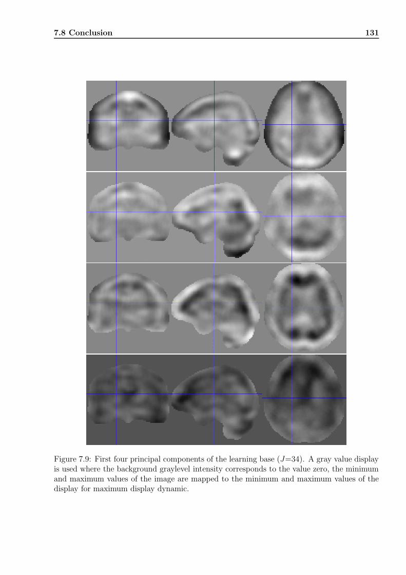
7.8 Conclusion 131
Figure 7.9: First four principal components of the learning base (J=34). A gray value displayis used where the background graylevel intensity corresponds to the value zero, the minimumand maximum values of the image are mapped to the minimum and maximum values of thedisplay for maximum display dynamic.

132 Atlas creation, our approach
Figure 7.10: Learning base residual after removing four principal components. This is thesquare root of the diagonal of Σε in Eq. 6.1.
0
0.05
0.1
0.15
0.2
0.25
0.3
0.35
-2 0 2 4 6 8 10 12 14 16 18 20
Pro
babi
lity
Standard deviation
local modelPCA2PCA4PCA6PCA8
PCA10PCA12PCA14
Figure 7.11: Histogram of the learning base residual images with increasing number of eigen-vectors, starting with the local model (Fig. 7.7), the mean of curves move to the left withincreasing number of principal components. The histogram of Fig. 7.10 is the third curvefrom the right (PCA4). Note that the residual for the global model was calculated using thereduced number of degrees-of-freedom as in Eq. 6.1. These curves do however hide some ofthe structure in the images: in the learning base residual of the model PCA14 for example, wefound regions of higher variance than in the model PCA1 even though the average variancehas dropped.

7.8 Conclusion 133
Var
2
-2.0
-1.5
-1.0
-0.5
0.0
0.5
1.0
1.5
Var 1
-2.0 -1.5 -1.0 -0.5 0.0 0.5 1.0 1.5 2.0
Var
3
-2.0
-1.5
-1.0
-0.5
0.0
0.5
1.0
1.5
2.0
Var 1
-2.0 -1.5 -1.0 -0.5 0.0 0.5 1.0 1.5 2.0
Var
4
-2.0
-1.5
-1.0
-0.5
0.0
0.5
1.0
1.5
2.0
Var 1
-2.0 -1.5 -1.0 -0.5 0.0 0.5 1.0 1.5 2.0
Var
5
-2.0
-1.5
-1.0
-0.5
0.0
0.5
1.0
1.5
2.0
2.5
3.0
Var 1
-2.0 -1.5 -1.0 -0.5 0.0 0.5 1.0 1.5 2.0
Var
3
-2.0
-1.5
-1.0
-0.5
0.0
0.5
1.0
1.5
2.0
Var 2
-2.0 -1.5 -1.0 -0.5 0.0 0.5 1.0 1.5
Var
4
-2.0
-1.5
-1.0
-0.5
0.0
0.5
1.0
1.5
2.0
Var 2
-2.0 -1.5 -1.0 -0.5 0.0 0.5 1.0 1.5
Var
5
-2.0
-1.5
-1.0
-0.5
0.0
0.5
1.0
1.5
2.0
2.5
3.0
Var 2
-2.0 -1.5 -1.0 -0.5 0.0 0.5 1.0 1.5
Var
4
-2.0
-1.5
-1.0
-0.5
0.0
0.5
1.0
1.5
2.0
Var 3
-2.0 -1.5 -1.0 -0.5 0.0 0.5 1.0 1.5 2.0
Var
5
-2.0
-1.5
-1.0
-0.5
0.0
0.5
1.0
1.5
2.0
2.5
3.0
Var 3
-2.0 -1.5 -1.0 -0.5 0.0 0.5 1.0 1.5 2.0
Figure 7.12: Learning base images in subspace. Projections onto two-dimensions for visu-alization of the learning base distribution in the space spanned by the first five principalcomponents (denoted Var q, q ∈ [1, 5] in this figure).

134 Atlas creation, our approach

Chapter 8
Atlas evaluation
One of the main difficulties linked to the creation of a brain perfusion atlas is its assessment, i.e.how well does the atlas describe normality and how sensitive is it at detecting abnormalities?In this chapter we present an evaluation study based on a leave-one-out strategy combined withsimulated abnormalities. This evaluation aims at making statements about both the model-fitand the detection performance of the different models considered in this work. Furthermore, itprovides a powerful way of evaluating and comparing different registration schemes. With thisscheme we could show that the registration scheme presented in Sec. 7.3 indeed yielded thebest results. Furthermore, a slightly better performance of the standard PCA model (“global”model) over the univariate Gaussian model (“local”model) was found for small abnormalities.A superior performance of the robust PCA models (with and without subspace modeling) overthe other models for large abnormalities was also found. However, there were no differencesbetween the performances of the robust PCA model and the robust PCA model with non-parametric subspace modeling. See also [219] and [221].
8.1 The need for validation
The importance and potential benefits of validation can be seen in Fig. 1.2, p. 5. Validationcan highlight intrinsic characteristics of a method, define its limits, and clarify the clinicalpotential of a method. Furthermore, it can help the development of better methodology byclearly defining requirements and improve the understanding of the problem domain (from atechnological viewpoint). As Russell H. Taylor1 pointed out at a recent talk in Strasbourg,industry has a lot of competence in validating methods and systems. Such competence is alsonecessary and useful in academia. Validation of new methods will determine whether suchmethods can find an application or not. A recent editorial in IEEE Transactions on MedicalImaging [112] highlighted this issue. Here, the authors brought validation of medical imageanalysis/synthesis research into a broader perspective. Validation is needed at several levelsand there is a need to develop standard terminology, as well as common, rigorous methodolo-gies. We shall not continue the discussion on standardization, but focus on difficulties relatedto the validation of the image processing methods we have used. These difficulties motivatedthe particular evaluation strategy that we have adopted. We continue by presenting otherrelevant evaluation studies before we present our study together with the results we haveobtained.
1Professor at the John Hopkins University and director of the Computer Integrated Surgical Systems andTechnology research center, Maryland, USA.

136 Atlas evaluation
8.2 The difficulty of validation
The approval of methods for clinical use is in most countries performed by randomized andblinded multicenter clinical trials. This is costly and time consuming so that for journalpublications, researchers typically show the feasability of a method or perform comparativestudies. Further difficulties are linked to the complexity of a system or an algorithm to bevalidated (e.g. registration). This complexity can for example manifest itself as many possibleparameter settings. If such parameters are correlated, an exhaustive validation across allpossible parameter settings may be necessary, but impossible in practice. However, the mainproblem for the validation of medical image processing techniques, is the uncertainty aboutwhat is correct (and not correct). This is the problem of a missing “ground truth” or “goldstandard”. For example, for a brain perfusion atlas, we acquire images of subjects we assumeto be normal, and who we ask to refrain from performing any particular brain task duringinjection. Such statements can only be true to a certain degree. Further complications forthe validation, evaluation and comparison of methods are the lack of standardized databases,algorithms, software, methodology and terminology (see also [112]).
As another example let us consider the validation of registration, which is central to theatlas creation process. We mentioned in Sec. 6.4.3 that the validation of registration meth-ods is extremely difficult. This is because we do not know the true parameters of a goodregistration nor if the deformation model is actually valid. As discussed in [226] a homologybetween different subjects may not exist and transformations can be overparametrized. Vi-sual assessment of registration methods by superimpositioning of the registered images is notsufficient to conclude on the validity of the transformation. Simulated deformations may notbe a valid assessment criterion since they are necessarily model-based (however useful in thedevelopment of the method). The authors also evoke the difficulty of defining a validationmetric, even when the ground truth is known, i.e. quantifying a good registration. One of themost complete comparison/evaluation studies of inter-subject, MRI registration algorithms isthe study in [94], where the authors have used several similarity measures to compare theregistration quality. They do however state that the “ideal” transformation depends on theapplication.
8.2.1 Validating model hypotheses
Statistical tests of goodness-of-fit
Validating a model means that we want to assess a hypothesis about the model. As emphasizedin [112], such hypotheses should be stated clearly and preferably be standardized (e.g. tofacilitate meta-analysis). An example of such an hypothesis could in our case be: The countvalues in brain SPECT images are normally distributed according to the linear model Eq. 4.1when anatomical structures are superimposed and when global differences due to variations inthe injected dose are removed. Statistical goodness-of-fit tests have indeed been developed toassess this kind of hypothesis. We could apply multivariate tests of normality [148], but thesample size (J = 20) is too small to yield meaningful results [72]. Another possibility wouldbe to test marginal probabilities by applying a Kolmogorov-Smirnov or a Lilliefors test ateach voxel. This is also problematic because one would need to interpret the results (e.g. isit reasonable to obtain rejections in 10% of all voxels, given the spatial correlations in thedata?), the sample size is still small, and finally, we expect a relatively simple model like thisto be rather approximate (we would therefore want to know “how approximate” the model

8.2 The difficulty of validation 137
is). Furthermore, in order to know anything about the power of the goodness-of-fit test, onewould need to formulate an alternative hypothesis (the power of a test is 1 − β, where β isthe probability of false negatives). Formulating a specific alternative hypothesis is difficult.Another formulation for an hypothesis could therefore be more tuned to the application ofthe model: The model [...above...] is accurate enough to detect abnormal lesions of a specifictype. However, here we encounter the problem of modeling the distribution of a pathology(This is generally accepted to be a more difficult problem than to model normality, see alsothe discussion of generic modeling in Sec. 3.2.5).
Empirical tests of goodness-of-fit: generalization
The above considerations have led us to abandon statistical goodness-of-fit tests, mainly be-cause of the small sample size. At the other extreme, as pointed out in [194, p.143], almostany goodness-of-fit test will fail for sample sizes that are large enough when the hypothesizeddistribution is only “almost true”. In pattern recognition, it is rather usual to consider a distri-bution as approximate2, and a more practical view on the goodness-of-fit for a model is taken:generalization. Generalization is a measure of how well a classifier performs on unseen dataand is also useful for examining the performance of non-statistical methods. Such an evalua-tion is done by splitting data into training data (used for training or parameter estimation)and test data (that constitutes the unseen data). In situations where only small data sets areavailable, as is our case, one typically ressorts to a leave-one-out strategy. This is what wehave done as described in Sec. 8.5.
8.2.2 Evaluating the model and the influence of preprocessing al-gorithms
It is clear that the image processing steps taken to prepare the images for statistical modelingwill have an influence on its accuracy and validity. Thus, having found a way of evaluatingthe statistical model, one is intuitively taken to examine this influence. This is attractivebecause, as we have discussed in Sec. 8.2, a complex algorithm like deformable registrationis difficult to validate. If one considers that the atlas model is (approximately) valid, oneexpects a “good” registration to yield a “good” atlas. We therefore suggest that the atlasperformance is a powerful criterion for comparing different registration methods (with respectto the application of atlas or group analysis).
Let us discuss this conjecture. First, recall that the atlas describes variability in a pop-ulation after image registration. The variation observed in a population is often consideredto stem from two different and independent sources, namely (1) anatomical variability and(2) functional variability. It is likely that the two sources of variability add up rather thancompensate each other. When we say an atlas is “good”, we mean that the variability of thepopulation is described with high fidelity. This fidelity is obtained by an accurate model. Webelieve that a good registration will improve the accuracy of the model because (1) it reducesthe anatomical variability, and (2) the anatomical variability is highly non-linear, violating ourlinear model hypothesis. It is furthermore often hypothesized that the localization of basicbrain functioning is strongly correlated with the anatomical structure of the brain (this is
2The Irish statistican Roy Geary (1896 - 1983) is attributed the following phrase [148, p. 279]: ’“Normalityis a myth; there never was, and never will be a normal distribution”. This is an overstatement from thepractical point of view, but it represents a safer united mental attitude...’

138 Atlas evaluation
SPECT brain segmentation
SPECT intensitynormalization
Intra-subjectSPECT-MRIregistration
Inter-subjectMRI-MRI
registration
Statistical model
SPECT imageacquisition
Figure 8.1: Independence diagram for different image processing units and the statisticalmodel. The solid lines show the main influence paths between units, and dashed arrows showless important influence paths. Image acquisition and reconstruction parameters (attenua-tion correction, scatter correction, etc.) certainly have a significant influence on inter-subjectregistration, normalization and the statistical model, but are out of the scope of this thesis.Furthermore, we found that the SPECT brain segmentation had a small effect on the cal-culation of principal components. However, this effect was negligible for a range of visuallyacceptable segmentations. Inter-subject, MRI registration has an influence on the joint his-togram that is used for intensity normalization (but is less important for other normalizationmethods). Given the simple (linear) transfer function used for normalization, we consideredthis influence also to be negligible. This leaves a graph where the registration algorithms andintensity normalization can be considered to be independent (given the SPECT images).
probably not so for higher cognitive brain functioning). Removing anatomical variability willtherefore leave, in theory, only functional variability which is exactly what we seek to study.
In order to evaluate the influence of the parameters of a method (preprocessing algorithmsin this case), it is important to understand their inter-relations and mutual dependencies. Apowerful and convenient way of doing so is to consider an independence diagram3, an exampleof which is shown in Fig. 8.1. We see that the different units influence each other, but we canconsider the registration and intensity normalization to be relatively independent parameters.This justifies the examination of the influence of, for example, normalization under a fixedregistration.
3Independence diagrams are a graphical way of expressing the conditional independence relationships amonga set of random variables (or abstractions of these) [164, 155]. Such diagrams thus permit one to easily readconditional independences.

8.3 Evaluation studies based on simulations 139
8.3 Evaluation studies based on simulations
Other simulation studies for assessing methods that characterize cerebral lesions in SPECT andPET images have been described. In [197], the authors decrease and increase the perfusion ona sphere in the right frontal lobe of the mean image to evaluate the capacity of SPM (statisticalparametric mapping) to detect changes. We think this approach yields an optimistic estimatebecause an abnormality can vary in an additive manner around the variation of normal images,not only around their mean. Furthermore, the study is limited to only one location of theabnormality whereas we show that the detection sensitivity of the atlas is location-dependent.Another study [128] adds inclusions to a software phantom, thereby simulating a single-subjectactivation study, whereas we are more concerned with multiple individuals with “activations”in out-of-group subjects. In [158], the authors compare SPM and the computerized brainatlas (CBA) [83] for PET activation studies using both human volunteers and simulations.The synthesized images are also derived from a single (simulated) PET image. Our contextis somewhat different from a standard activation study with multiple conditions/multiplesubjects: we have several control images in rest state (learning set) and only one activationimage of a subject that is not represented in the learning set. Another study also comparesthe effects of different registration and filtering algorithms on the detection capacity of SPMby simulating PET images [50]. These are simulated from the MR images, but this time from16 different persons. This way natural anatomical variance is present in the database, but thefunctional variance still lacks.
All of these studies are biased since the resting state/inactive images of the person(s) beingstudied are present in the learning base. This is of course the way most activation studiesare designed (especially in cognitive tasks), but such images are not available in real-worldatlas-patient comparisons. Because of the cross-validation design of the proposed evaluationstudy, it is not biased in this manner. The influence of using an unbiased evaluation strategyis further discussed in Sec. 8.6.6.
8.4 Evaluation in the absence of a ground truth
Recently a class of methods have caught the attention of researchers working on the devel-opment and validation of new medical imaging technologies [101, 125, 114]. These are calledlatent class analysis methods (or are related to these). Latent class analysis is interesting be-cause it allows us to compare different methods in the absence of a “gold standard” or “groundtruth”. In medical imaging this is often the case either because it is very expensive, invasiveor impossible to obtain a gold standard.
In a simple binary detection scenario (pathology or not), the quality of a method is charac-terized by its sensitivity, specificity and the prevalence (probability of pathology). The basicidea is that applying several tests (methods) on several populations and matching the results,yields enough degrees of freedom to estimate the sensitivity and specificity of each method.
In the more complex cases of estimating covariates (continuous variables, e.g. regionalcerebral blood flow), models similar to the factor analysis model (and the models used in thiswork) have been used [125, 114]. Here again, the models can be compared indirectly, that iswithout knowing the ground truth. We have not had the opportunity to study any of thesemethods in this work. To our knowledge there have not been any studies that have used suchmethods to compare voxel-based statistical atlases yet. We believe though, that latent classanalysis will become more important to the image processing community in the future.

140 Atlas evaluation
Baseimage
Modelestimation
+/-Comparison
Atlas
Results
DB
Ground truth Score image
Learning Set
Test image
Add inclusion
ROCanalysis
Figure 8.2: Schematic view of the leave-one-out strategy employed. At every iteration abaseimage is removed from the database (DB) from which a test image is synthesized byintroducing inclusions in the baseimage (see Fig. 8.3). The atlas is constructed from theremaining images and the comparison yields the score image. A good atlas describes thebaseimage well and is sensitive enough to detect the inclusions. The procedure is repeated forall images in the DB and the results are averaged to measure the overall performance. Weused inclusions at six different locations, of two sizes and six intensities, so that we obtaineda total set of 72 score images for every baseimage. The database contained 34 images.
8.5 Proposed evaluation scheme
An overview of the validation procedure can be seen in Fig. 8.2. The different processing stepswill now be outlined before we describe the evaluation criterion.
Leave-one-out
The leave-one-out methodology is a standard method in pattern classification used to estimatethe generalizing power of a method when only a small dataset is available [58]. Given a datasetof size J , our leave-one-out scheme simply consists of iterating the procedure depicted in Fig.8.2: remove an image from the learning set, estimate the model, create a test image, comparethis image to the estimated model. A score image and its corresponding ground truth isthus created for each image of the J dataset images. Using ROC analysis (receiver operatingcharacteristics), the performance is then estimated by averaging the results of all these images.It is a rather time consuming technique, but the only one appropriate when data acquisition
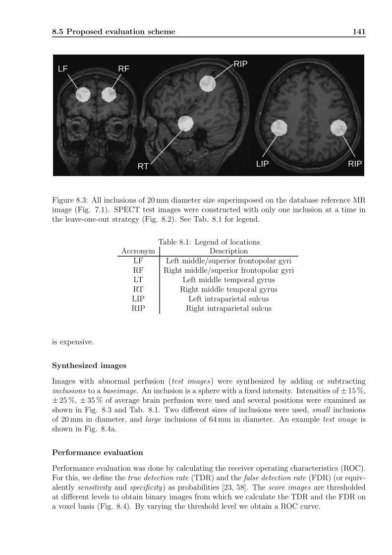
8.5 Proposed evaluation scheme 141
LF RF
RT
RIP
LIP RIP
Figure 8.3: All inclusions of 20mm diameter size superimposed on the database reference MRimage (Fig. 7.1). SPECT test images were constructed with only one inclusion at a time inthe leave-one-out strategy (Fig. 8.2). See Tab. 8.1 for legend.
Table 8.1: Legend of locationsAccronym Description
LF Left middle/superior frontopolar gyriRF Right middle/superior frontopolar gyriLT Left middle temporal gyrusRT Right middle temporal gyrusLIP Left intraparietal sulcusRIP Right intraparietal sulcus
is expensive.
Synthesized images
Images with abnormal perfusion (test images) were synthesized by adding or subtractinginclusions to a baseimage. An inclusion is a sphere with a fixed intensity. Intensities of ± 15%,± 25%, ± 35% of average brain perfusion were used and several positions were examined asshown in Fig. 8.3 and Tab. 8.1. Two different sizes of inclusions were used, small inclusionsof 20mm in diameter, and large inclusions of 64mm in diameter. An example test image isshown in Fig. 8.4a.
Performance evaluation
Performance evaluation was done by calculating the receiver operating characteristics (ROC).For this, we define the true detection rate (TDR) and the false detection rate (FDR) (or equiv-alently sensitivity and specificity) as probabilities [23, 58]. The score images are thresholdedat different levels to obtain binary images from which we calculate the TDR and the FDR ona voxel basis (Fig. 8.4). By varying the threshold level we obtain a ROC curve.

142 Atlas evaluation
(a) (b) (c) (d)
Figure 8.4: A transversal slice of (a) a test image with an inclusion of 25% of average brainperfusion in the right frontal lobe (RF), (b) the score image, (c) the thresholded score image,which is compared to (d) the ground truth image in order to determine the FDR and TDRrates.
The FDR and TDR are calculated as follows: For a given threshold, let δ(j)k take on the
value 1 for detection (value above threshold) at voxel k in subject j = 1, . . . , J and 0 fornon-detection and let I designate the 3D region defined by the inclusion. We then define theTDR at this threshold as
TDR =
∑Jj=1
∑
i∈I δ(j)i
∑Jj=1
∑
i∈I 1(8.1)
and FDR as
FDR =
∑Jj=1
∑
i∈B\I δ(j)i
∑Jj=1
∑
i∈B\I 1, (8.2)
where B is the region defined by the brain (we use the same brain mask as for PCA). It isimportant to note the outer sum: it is not valid to calculate ROC curves for each image andsum these, each pair of FDR/TDR must be calculated for a fixed threshold across all theimages.
Since the definition of the false detection rate does not make any distinction between“good”and“bad”false alarms, one might discuss whether these ROC curves are appropriate or not. Incertain pathologies, the physicist is only concerned by grossly identifying an atrophical regionor just lateralize abnormal brain perfusion (qualitative evaluation). However, the advantageof such a measure is that it provides an objective result.
Significance testing of differences
In order to assess the statistical significance of the difference between two curves, we summa-rized the ROC curves by estimating the partial area under the curve (AUC). Only the partialAUC, denoted AUC0.05, in the range of FDR ∈ [0, 0.05] was calculated since a FDR of 0.05already represents a large quantity of voxels (about 1000 voxels as compared to the smallinclusions that are 110 voxels). Furthermore, the standard error of the AUC0.05 estimates wasestimated using the jackknife (“leave-one-out”) technique as described in [58, p. 473]. Thiserror was then used to assess the significance of the difference between two curves. For this a

8.6 Results and discussion 143
z-score [88]AUC1 − AUC2
SE, (8.3)
is calculated, where SE is the standard error and the subscripts denotes the two resultsobtained with two different methods (model, registration) or on two different locations. Thez-score is compared to a normal distribution table in order to obtain a p-value. When there isreasonable evidence for postulating an alternative hypothesis where one particular method isbetter than another (e.g. robust global better than global), a one-sided value (one tail of thenormal distribution) can be used. Otherwise, when the alternative hypothesis is that the twomethods are different, a two-sided value must be used (twice the one-sided value).
Furthermore, in Eq. 8.3, the standard error depends on what is actually compared. Whentwo methods are compared whose results stem from different sample sets, we have that SE =√
SE21 + SE2
2 . This is the appropriate standard error to use when comparing for example theperformance on two different locations. However, when the underlying sample sets are thesame, as they are when we compare models (local, global and robust global) or preprocessingsteps (registration, intensity normalization), a correlation corrected standard error can be usedas explained in [89]:
SE =√
SE21 + SE2
2 − 2rSE1SE2.
The justification for this is analogous to the use of the paired t-test instead of an unpaired t-testand can increase the statistical power of the test considerably: fluctuation of the ROC curves(and the accuracy index AUC) will tend to fluctuate in tandem when derived from the samesample. Unfortunatly, the correlation coefficient, r, in this equation is not derived analytically,but is only tabulated in [89]. It depends on the correlation of the true negative/positive scoresobtained by the two methods, as well as the AUC of the two methods. Furthermore, it isbased on the assumption of a binormal distribution of the true negative and positive scores.In our experiments, the correlation coefficient was found to lie between 0.7 and 0.8, dependingsomewhat on the intensity of the inclusion (since this changed the AUC considerably).
8.6 Results and discussion
If not stated otherwise, all results were obtained using the deformable registration scheme(Deform6-F) described in Sec. 7.3.3 and the total least squares intensity normalization asdescribed in Sec. 7.5. We first compare models using small inclusions (20mm ∅), then usinglarge inclusions (64mm ∅). We then compare registration schemes and show the overall im-provement of our approach over the more common atlas approach (affine registration, averagenormalization and local model). Finally, we describe the location specific results. Only arepresentative subset of hypo-inclusions are reported. The results for hyper-inclusions yieldedsimilar results and the conclusions are similarly valid for these.
8.6.1 Comparing models
Small inclusions
In Fig. 8.5 are depicted the ROC curves for the local model and the global model usingsmall inclusions. The curves were obtained by averaging over all locations and with a varyingnumber of eigenvectors for the global model. The standard errors of these curves were alsoestimated as described in Sec. 8.5 and the significance levels of the differences between any

144 Atlas evaluation
0
0.2
0.4
0.6
0.8
1
0 0.005 0.01 0.015 0.02 0.025 0.03 0.035 0.04 0.045 0.05
TD
R
FDR
-25%
-15%
LocalPCA1PCA2PCA3PCA4
Figure 8.5: Comparison of models. Local is the local model, PCAq is the global model using qprincipal components. ROC curves averaged over all locations. The curves were obtained forsmall hypo-inclusions (20mm ∅) with intensities of 15% and 25% of average brain perfusion.Similar curves were obtained for the other intensities studied. Significance values are given inTab. 8.2.
two curves are tabulated in Tab. 8.2 for the 25% hypoperfusions. Here we see that the PCA2-PCA4 models are all significantly above the local and PCA1 models. The difference betweenthe local and the PCA1 model on one hand and the difference between the PCA3 and PCA4models are however not significant. With an odds of about 1:6 (1:7), the difference betweenthe PCA3 (PCA4) model and the PCA2 model is not very significant.
In this paper we quantify the accuracy of different models and we show for the first timethat the global model of Houston et al. performs significantly better than the local model asseen in Fig. 8.5 and Tab. 8.2. This is true for the model with 2, 3 and 4 eigenvectors. Theappropriate choice of number of eigenvectors is however quite difficult. Too few componentslimit description power and too many may result in overfitting [58, 91] yielding eigenimages or
Model PCA1 PCA2 PCA3 PCA4Local 0.9972 0.0061 0.0001 0.0001PCA1 0.0045 0.0001 4.24E-5PCA2 0.1567 0.1398PCA3 0.9254
Table 8.2: Two-sided p-values associated with the 25% hypo-inclusions in Fig. 8.5. Forexample, one can see that the odds that the PCA3 model is different from the local model onlyby chance are 1 : 10000 (second row, fourth column). Since the PCA3 model shows a betterROC curve in Fig. 8.5, we therefore conclude that this model’s performance is significantlybetter than that of the local model.

8.6 Results and discussion 145
0
0.2
0.4
0.6
0.8
1
0 0.005 0.01 0.015 0.02 0.025 0.03 0.035 0.04 0.045 0.05
TD
R
FDR
-25%
-15%
LocalPCA3
Robust-PCA3
Figure 8.6: ROC curves averaged over all locations. The curves were obtained for large hypo-inclusions (64mm ∅) with intensities of 15% and 25% of average brain perfusion. Note thatthe effective size of the inclusions were inferior to the volume of the sphere because regionsoutside the brain covered by the sphere was ignored.
-patterns that are specific of the sample images, not of the underlying distribution. Both caseslead to lower model performance. In Tab. 8.2, we see that between the models with 3 and4 eigenvectors there is no significant difference (bottom-right entry), whereas these two areonly moderately different from the PCA2 model. That covariance patterns in one or severalpopulations carry useful information has also been shown in other studies [115, 179]. Notehowever, that we do not interpret these patterns, they merely serve as complex descriptors ofnormal variation.
Large inclusions
In Fig. 8.6 are depicted the ROC curves obtained using large inclusions. Whereas for smallinclusions, the global model and the robust global model yield the same results, this is nolonger the case when the size of abnormalities becomes larger. By design, the robust model(Robust-PCA3) will always be at least as good as the global model, which justifies one-sidedp-values for comparing these two models. These are 0.0061 and 0.1044 for the 25% and the15% hypo-perfusions respectively. The differences between the PCA3 and the local modelhave two-sided significance values as p < 0.0078 and p < 0.0671 for the 25% and the 15%hypo-perfusions respectively.
In realistic cases the zones of abnormal perfusion might be large or small. The robustmodel showed better results for large abnormalities than the other models (Fig. 8.6) and hadequal performance for small inclusions. With increasingly good model description, due to amore representative database and better preprocessing, we expect the model to show evenclearer advantages over the local and standard global model. This is observed in Fig. 8.7,which is a result from a pilot study. We synthesized test images from a baseimage which was

146 Atlas evaluation
0.94
0.96
0.98
1
0 0.1 0.2 0.3
Rob. r=3
♦
♦Ortho. r=3
+
+ +0.2
0.4
0.6
0.8
1
0 0.1 0.2 0.3
Rob. r=6
♦♦♦♦♦
♦
♦Ortho. r=6
+++++
+
+
+ +
0.2
0.4
0.6
0.8
1
0 0.1 0.2 0.3
Rob. r=9
♦♦♦♦♦♦
♦
♦♦
Ortho. r=9
++++
++++++
+0
0.2
0.4
0.6
0.8
1
0 0.1 0.2 0.3
Rob. r=12
♦♦♦♦♦♦
♦
♦
♦Ortho. r=12
+++
++
+++++ +
Figure 8.7: The receiver operating characteristics (ROCs) for images composed of an imagefrom the learning base with different inclusions. Four different spherical inclusions of ra-dius=3,6,9 and 12 voxels were added and a model with the first 12 principal components thataccounts for about 93 percent of the total variance in the learning base was used. (Rob. ishere the RML model, Ortho. the ML global model.)
included in the learning set. Using 12 principal components, the baseimage was thus fairly wellmodeled. With increasing size of the inclusions we see that the performance of the standardPCA model drops significantly. This is the same kind of improvement that we have observedin our experiments on manufactured objects, Ch. 5.
8.6.2 Comparing registration schemes
Fig. 8.8 shows the results obtained using different registration schemes. These schemes wereexplained in Sec. 7.3.3. All differences are significant (Deform6-F vs. Affine: p < 0.0046,Affine vs. Deform3 p < 0.0033, and Deform3 vs. Deform6-NF is negligible), again usingtwo-sided p-values.
An influential factor on voxel-based, inter-subject studies is undeniably the spatial normal-ization or registration (Fig. 8.8) [225]. Since the assumption is that only similar structuresshould (grossly) yield comparative functional signals, these must be correctly superimposed.The leave-one-out strategy presented in this paper is clearly valid for comparing differently reg-istered, normal images under this assumption. However, this is not true as to the algorithmscapacity of registering abnormal images since these have been simulated after registration.The best results were obtained with the deformable registration scheme and filtering of thedeformation field. In this study we have shown that a linear 12-parameter affine registrationas is often used [1], is less performant than deformable co-registration. However, this approachis only possible when both SPECT and MR images of the patient are available. Finally, wenotice that these conclusions are in contradiction to those found by Crivello et al., where theyconclude that the registration has low influence on low resolution images [44].
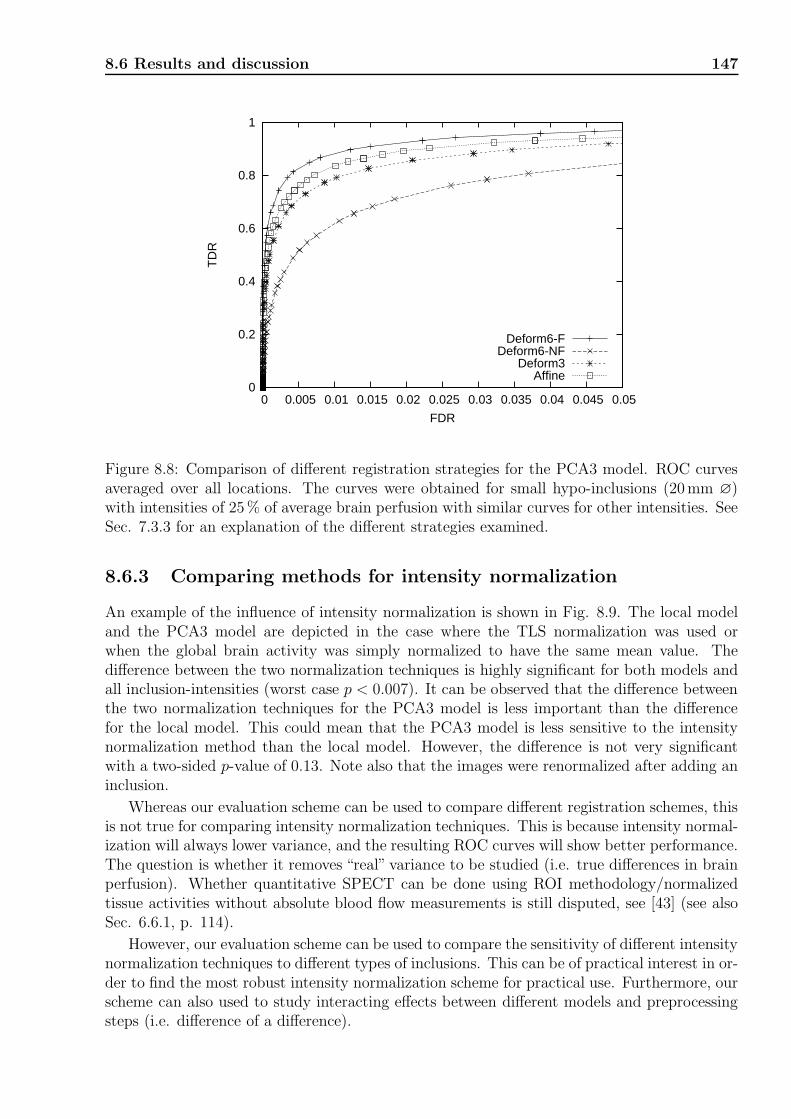
8.6 Results and discussion 147
0
0.2
0.4
0.6
0.8
1
0 0.005 0.01 0.015 0.02 0.025 0.03 0.035 0.04 0.045 0.05
TD
R
FDR
Deform6-FDeform6-NF
Deform3Affine
Figure 8.8: Comparison of different registration strategies for the PCA3 model. ROC curvesaveraged over all locations. The curves were obtained for small hypo-inclusions (20mm ∅)with intensities of 25% of average brain perfusion with similar curves for other intensities. SeeSec. 7.3.3 for an explanation of the different strategies examined.
8.6.3 Comparing methods for intensity normalization
An example of the influence of intensity normalization is shown in Fig. 8.9. The local modeland the PCA3 model are depicted in the case where the TLS normalization was used orwhen the global brain activity was simply normalized to have the same mean value. Thedifference between the two normalization techniques is highly significant for both models andall inclusion-intensities (worst case p < 0.007). It can be observed that the difference betweenthe two normalization techniques for the PCA3 model is less important than the differencefor the local model. This could mean that the PCA3 model is less sensitive to the intensitynormalization method than the local model. However, the difference is not very significantwith a two-sided p-value of 0.13. Note also that the images were renormalized after adding aninclusion.
Whereas our evaluation scheme can be used to compare different registration schemes, thisis not true for comparing intensity normalization techniques. This is because intensity normal-ization will always lower variance, and the resulting ROC curves will show better performance.The question is whether it removes “real” variance to be studied (i.e. true differences in brainperfusion). Whether quantitative SPECT can be done using ROI methodology/normalizedtissue activities without absolute blood flow measurements is still disputed, see [43] (see alsoSec. 6.6.1, p. 114).
However, our evaluation scheme can be used to compare the sensitivity of different intensitynormalization techniques to different types of inclusions. This can be of practical interest in or-der to find the most robust intensity normalization scheme for practical use. Furthermore, ourscheme can also used to study interacting effects between different models and preprocessingsteps (i.e. difference of a difference).
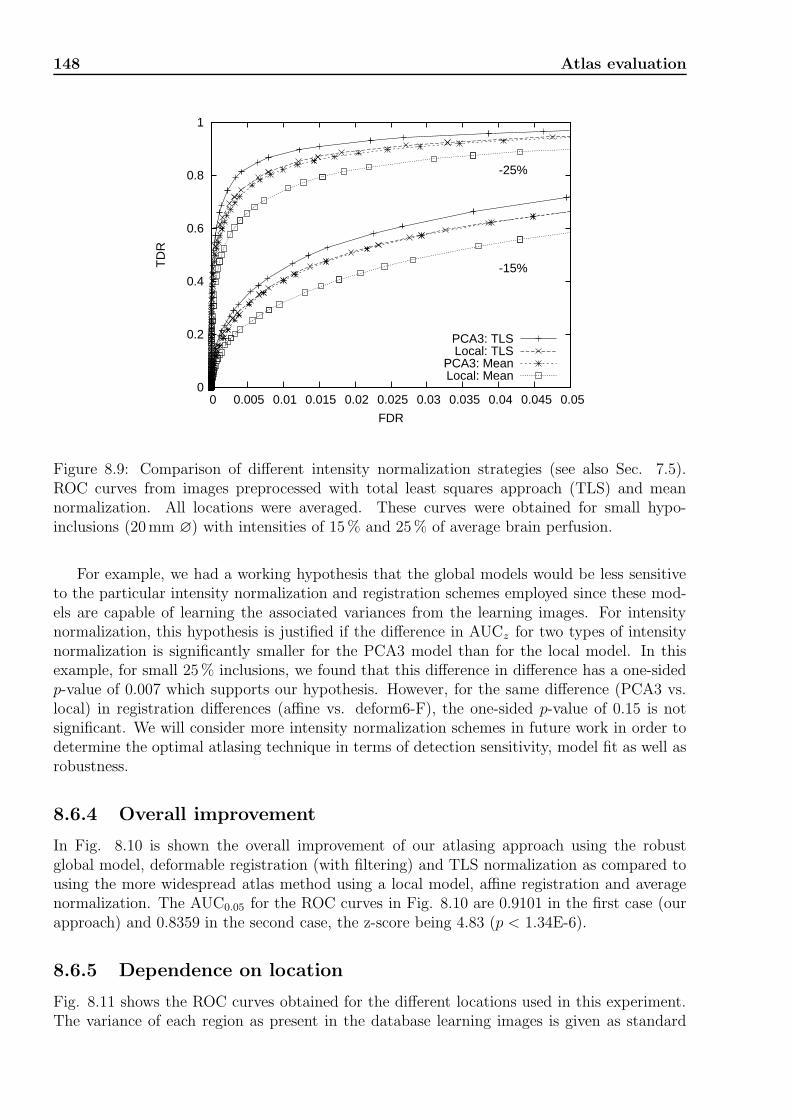
148 Atlas evaluation
0
0.2
0.4
0.6
0.8
1
0 0.005 0.01 0.015 0.02 0.025 0.03 0.035 0.04 0.045 0.05
TD
R
FDR
-25%
-15%
PCA3: TLSLocal: TLS
PCA3: MeanLocal: Mean
Figure 8.9: Comparison of different intensity normalization strategies (see also Sec. 7.5).ROC curves from images preprocessed with total least squares approach (TLS) and meannormalization. All locations were averaged. These curves were obtained for small hypo-inclusions (20mm ∅) with intensities of 15% and 25% of average brain perfusion.
For example, we had a working hypothesis that the global models would be less sensitiveto the particular intensity normalization and registration schemes employed since these mod-els are capable of learning the associated variances from the learning images. For intensitynormalization, this hypothesis is justified if the difference in AUCz for two types of intensitynormalization is significantly smaller for the PCA3 model than for the local model. In thisexample, for small 25% inclusions, we found that this difference in difference has a one-sidedp-value of 0.007 which supports our hypothesis. However, for the same difference (PCA3 vs.local) in registration differences (affine vs. deform6-F), the one-sided p-value of 0.15 is notsignificant. We will consider more intensity normalization schemes in future work in order todetermine the optimal atlasing technique in terms of detection sensitivity, model fit as well asrobustness.
8.6.4 Overall improvement
In Fig. 8.10 is shown the overall improvement of our atlasing approach using the robustglobal model, deformable registration (with filtering) and TLS normalization as compared tousing the more widespread atlas method using a local model, affine registration and averagenormalization. The AUC0.05 for the ROC curves in Fig. 8.10 are 0.9101 in the first case (ourapproach) and 0.8359 in the second case, the z-score being 4.83 (p < 1.34E-6).
8.6.5 Dependence on location
Fig. 8.11 shows the ROC curves obtained for the different locations used in this experiment.The variance of each region as present in the database learning images is given as standard

8.6 Results and discussion 149
0
0.2
0.4
0.6
0.8
1
0 0.005 0.01 0.015 0.02 0.025 0.03 0.035 0.04 0.045 0.05
TD
R
FDR
Local, Affine, MeanRobust-PCA3, Deform6-F, TLS
Figure 8.10: Overall improvement of our atlasing approach that consists of deformable regis-tration, total least squares intensity normalization and a robust global model as compared tothe more usual approach that consists of affine registration, mean intensity normalization andthe local model. Results are averaged over all locations using small 25% hypo-inclusions.
Location RF LT RT LIP RIPLF 0.0003 0.0024 0.0935 0.3036 0.2463RF 2.62E-8 2.60E-6 0.0108 1.32E-5LT 0.2117 0.0005 0.0759RT 0.0155 0.6146LIP 0.0463
Table 8.3: Two-sided p-values associated with the 25% inclusions in Fig. 8.11.
deviations in parenthesis. The significance values corresponding to Fig. 8.11 is given in Tab.8.3. We see that the abnormalities are more difficult to detect in the right frontal region(RF) than in the other regions (p < 0.0108 or less). The difference between the right andleft curves is highly significant in the frontal region (p < 0.0003), significant in the parietalregion (p < 0.0463) and not significant in the temporal region. Averaging the right and leftregions and comparing regions, we have that the temporal region is easier for detection thanthe parietal region with significance p < 0.0339.
The asymmetry in variation found in the frontal cortex (Fig. 8.11) is in accordance witha higher uptake in this region as found in [127] as well as a known anatomical asymmetry inthe frontal lobe, the right being larger than the left in general [59, p.17]. The performancesobtained represent a combined measure of model-fit and detection sensitivity. The lowerperformance in the frontal region is therefore not only explained by a higher variance in thisregion, Fig. 8.11, but also reflects a limited capacity of the model to represent this region.For example is the average variance in the “LIP”-region (6.722) lower than in the “LF” region(7.982), even though the ROC curves show lower performance in that region (Fig. 8.11).

150 Atlas evaluation
0
0.2
0.4
0.6
0.8
1
0 0.005 0.01 0.015 0.02 0.025 0.03 0.035 0.04 0.045 0.05
TD
R
FDR
LF (7.98)RF (8.89)LT (5.44)RT (6.43)LIP (6.72)RIP (6.37)
Figure 8.11: Comparison of ROC curves for each location where inclusions were added usingthe PCA3 model. See Fig. 8.3 for legend. The curves were obtained for small hypo-inclusions(20mm ∅) with intensities of 25% of average brain perfusion. The curves were similar forother intensities. In parenthesis is given the average standard deviation in the area of theinclusion.
8.6.6 Comparing validation strategies
We already mentioned in Sec. 8.3 that none of the other evaluation studies have actually triedto validate the model hypotheses (i.e. that the data is normally distributed). This is becausethey use a biased strategy where the baseimage is included in the learning set. These studiestherefore yield optimistic performance estimates of the methods/models they validate. To seethe influence of the choice of validation strategy, we repeated the validation study, but thistime by leaving the baseimage in the learning set. The testimages were created in the samemanner as in the leave-one-out scheme, with the same locations and intensities. The resultsare shown in Fig. 8.12. We see that the biased estimates are clearly superior to the unbiasedestimates. It is clear that using the biased estimation method, we can obtain quite impressiveresults by increasing the number of eigenvectors. This is shown in Fig. 8.13 and is the reasonwhy we believe this model will be more performant than the local model for a representativedatabase of learning images that is more complete.
8.7 Conclusion
We do not expect a probabilistic, computerized atlas to replace visual inspection of SPECTscans. However, it can add value to SPECT examinations by permitting the comparison ofan image with normative data as we suggests in the next chapter. For this to be possible,complex image processing must be undertaken, whereby the impact and consequences of suchprocessing must be evaluated and well understood. Furthermore, the assumptions underlyingthe statistical models and tests must be validated. In this chapter, we have attempted to

8.7 Conclusion 151
0
0.2
0.4
0.6
0.8
1
0 0.005 0.01 0.015 0.02 0.025
TD
R
FDR
Local biasedLocal unbiased
PCA3 biasedPCA3 unbiased
Figure 8.12: Comparison of different validation strategies. The two upper curves are theperformances of the global and local models using a biased validation strategy where thebaseimage was part of the training set. The two lower curves are the performances usingthe leave-one-out strategy described in Sec. 8.5. All locations were averaged. The curveswere obtained for small hypo-inclusions (20mm ∅) with intensities of 25% of average brainperfusion.
0
0.2
0.4
0.6
0.8
1
0 0.005 0.01 0.015 0.02 0.025
TD
R
FDR
Local biasedPCA3 biasedPCA8 biased
Figure 8.13: With the biased validation strategy it is clear that we obtain increasingly betterROC curves with a higher number of principal components in the model (this is only true upto a certain limit). Here are shown three curves obtained for the local model, the global modelwith three and eight principal components respectively. Again, all locations were averaged.The curves were obtained for small hypo-inclusions (20mm ∅) with intensities of 10% ofaverage brain perfusion.

152 Atlas evaluation
obtain quantitative measures in this direction. Among the models studied, the robust (non-linear) global model shows the best overall characteristics: sensitivity, specificity and modelvalidity. This kind of model also compensates to some degree errors in registration and inten-sity normalization. However, we do not make any statements about the clinical outcome ofthese models or preprocessing algorithms.

Chapter 9
Clinical Application: Epilepsy
In the evaluation study presented in the last chapter, the capacity of the atlas and the dif-ferences between atlas models were evaluated in an exploratory setting, i.e. without a prioriinformation or hypotheses about the abnormality that is searched. In practice, this is nothow the physician works. He, or she, is interested in understanding more about the impactof an atlas in the routine analysis of SPECT images as well as its possible added value fordiagnostics.
In this chapter we present some preliminary results of comparing images of patients withepilepsy to the atlas. We begin by giving a brief introduction to epilepsy and the particularstatus of SPECT imaging for determining seizure foci. We proceed by discussing the addedvalue that we expect an supplementary analysis using the atlas could bring. We then finallypresent some results that are currently motivating further atlas-based projects.
9.1 The pathology
Brief description
Epilepsy is a brain disorder where patients have a tendency to experience recurrent seizures.An epileptic seizure happens when normal brain activity is disrupted and a number of neuronsstart firing signals in an uncontrolled manner. This may cause temporary changes in theperson’s personality, mood, memory, sensations, movement or consciousness. Seizures canbe classified into partial seizures or generalized seizures1. For partial seizures, a distinction ismade into simple and complex partial seizures, depending on whether a person’s consciousnessis impaired or not. A partial seizure may spread to involve the whole of the brain and thusturns into a (secondarily) generalized seizure. A generalized seizure begins with a widespreaddischarge that involves both sides of the brain at once.
Most people have seizures in their life, sometimes without even recognizing it. However,epilepsy is not diagnostized before at least two seizures have been observed. In only threeout of ten cases of epilepsy is it possible to find a cause. Causes include head injury, stroke,infections, brain tumors and others. In summary, one can say that epilepsy is a complexneurological disorder in which many pathophysiological aspects are not yet well understood.
1The classification of seizures is actually more complicated. This is only a typical, simplifiedcharacterization.
154 Clinical Application: Epilepsy
Treatment
About 80% of all cases of epilepsy are successfully treated with medicaments. The medica-ments aim at increasing the level of inhibitory neurotransmitters or at decreasing the amountof excitatory ones. Further treatments consists of a specialized (Ketonic) diet for children or avagus nerve stimulation (with an implant). However, in a small number of serious cases, whenother treatments fail, surgery is undergone. In partial epilepsy, the seizure center is removedfrom the brain. This can be done if the center is not situated in any essential part of thebrain (i.e. affecting speech-, memory-, audiovisual- or language cortex). Because of the highplasticity of the brain, the functions that were present in the removed region are taken overby other regions.
Four types of surgery are possible: (1) Temporal Lobectomy - here a part of or the wholetemporal lobe is removed. About 70% of the patients have marked improvement or are curedof their seizures. (2) Extratemporal Resections - seizure centers in an area other than the tem-poral lobe can sometimes be removed. Fifty percent of the patients have a marked reductionor elimination of their seizures. (3) Corpus Callosotomy - the interconnection between the twohemispheres is removed. This is only done in a very few patients having serious attacks andwhere many seizure centers are present. (4) Hemispherectomy - if one hemisphere of the brainis abnormal and causes seizures, it is completely removed in rare cases.
9.2 Medical imaging and epilepsy
From the above, it is clear that accurate localization of the seizure foci and brain functions isof utter importance for epileptic surgery. For this, several tests are available: neuropsychologicevaluation, Electroencephalogram (EEG), invasive EEG (also called stereotactic depth EEG,SEEG), Long Term Monitoring (LTM) with EEG and video surveillance, MR imaging to findmorphological atrophies, PET imaging for brain function and SPECT imaging of seizure onsetamong others. Typically, several tests are performed since they may yield complementaryinformation.
High-resolution MRI has emerged as the best diagnostic tool for identification of epilep-togenic lesion. In 20-40 % of patients with intractable epilepsy [205], no lesions are detectedon MRI. In these cases, invasive EEG studies are very useful. Invasive EEG studies have thedisadvantage of restrictive vision due to limited sampling and may not distinguish betweendistantly propagated seizures and initial discharge of the ictal onset zone. Occasionally, com-plications like hemorrhage and infections may also occur. Another aspect is that in developingcountries, facilities for invasive studies are not commonly available.
9.2.1 SPECT in epilepsy
Among the techniques for localizing seizure foci, SPECT imaging is in a particular positionbecause it is possible to image the seizure onset. For this the radiotracer is injected into thepatient at the moment of onset. Because the tracer is rapidly distributed to the brain (fixates)and remains trapped a few hours, it is possible to record images when the seizure is over andthe patient is calm. This is called an ictal image. A second interictal image is acquired of thepatient, either before or between seizures. These two images are then compared in order todefine the seizure focus (or foci) and eventually study the path of discharge.

9.3 Computer-aided evaluation and SISCOM 155
9.3 Computer-aided evaluation and SISCOM
In clinical practice, it is still quite common that an expert compares the two SPECT images(ictal and interictal) side-by-side. The images are typically displayed slice-by-slice in threedifferent views (coronal, axial and sagittal) and the expert has the possibiliy to scale theintensities (interactive intensity normalization). Furthermore, access to an interactive ROI(region of interest) method is provided, where the expert can delineate regions (typicallyusing simple geometrical forms such as ellipses) in the slices and compare mean values of theROIs.
To further improve the sensitivity of the detection of seizure foci, several automatic com-puter aided methods have been developed:
• Automatic intensity normalization.
• Intra-modal registration (using a rigid transformation model) that makes it possible tocreate subtraction images that highlight differences in the two images.
• Inter-modality registration with the patients MRI scan in order to improve the localiza-tion of the foci with respect to anatomical structures.
A method that combines these steps is known as SISCOM (Subtraction Ictal SPECT withCO-registered MRI) [237, 175, 176] and will be further discussed in the next section.
9.3.1 Intensity normalization revisited
As for intensity normalization, we have already discussed this issue at length in both Sec.6.6, p. 113 and in Sec. 7.5, p. 126. Because of the sometimes large modifications observedin ictal SPECT images with respect to normal images, several authors argue that speciallyadapted intensity normalization methods are necessary [22]. During a seizure, the blood flowcan become quite high and the uptake of tracer no longer depends linearly on the blood flow.Hyperperfused areas thus appear less intensely in the SPECT images as they actually are.Traditional intensity normalization techniques normalize the observed counts to the wholebrain uptake or to that of a (fixed) reference region. This is no longer useful for ictal imagessince the whole brain perfusion pattern can be completely altered. One technique that hasbeen specifically developed for intensity normalization of ictal and interictal SPECT imageshas been presented in [21] (also described in Sec. 6.6.3, p. 115). Here, the reference regionis automatically determined based on a criterion of homogeneity2. However, the technique isnot easily extensible to our case where we would like to compare ictal and interictal images toa database of normal images.
Another comparative study [185] recommends simple linear scaling based on the evaluationof the joint histogram (scatterplot) of the two images. Large zones of abnormal perfusion couldin this case lead to joint histograms where the distribution is non-linear, or equivalently, theregression line shows outlier concentrations. A possible solution in this case could be to userobust regression techniques such as those discussed in Sec. 3.5, p. 3.5 (or the one proposedin [185]). However, for this outlier effect to be of any impact, the number of abnormal voxelsmust be quite large. We have in practice never seen clear outliers in the joint histogram.What we have observed is on the contrary that the joint histogram between the ictal imageand the reference image is often more “smeared out” than the joint histogram between the
2Actually, two different criteria are proposed for finding this region.

156 Clinical Application: Epilepsy
interictal image and the reference image, see Fig. 9.1. This is probably the result of manymicro alteration of blood flow, both hypo and hyper. Because such smearing has less influenceon the estimate of the regression line than a large outlier concentration, we believe that thetotal least squares regression on the joint histogram is sufficiently robust also for the ictalimage. The only problem that we still think may be present is an underestimation of highblood flow values because the radioactive fixation may not necessarily linearly follow the bloodflow when these are high above what is normal.
Figure 9.1: Example joint histogram between a patient with epilepsy and the database refer-ence image. On the left: interictal image. On the right: ictal image. The histogram with theictal image is more smeared out than that for the interictal image.
9.3.2 Difficulties with SISCOM
The usefulness of the SISCOM technique is due to the availability of both the interictal imageand the ictal image. The interictal image thus serves as a reference image. In the interictalimage, one expects to find regions of hypoperfusion where the seizure foci is located, in theictal, zones of hyperperfusion. In fact, when PET exams are made, in which case one can onlyacquire an interictal image, zones of hypoperfusion are indicative of epileptic foci. However,these assumptions are not as simple in practice as discussed in [134] and illustrated in Fig.9.2. True interictal images are difficult to obtain, because the pathologic brain region issometimes hyperperfused several days after a seizure. A possible cause for this may be thatthe region needs to recover before blood flow again decreases to the patient’s normal level.Likewise, if the injection of the radiotracer does not comply perfectly with the seizure onset,the seizure center might be exhausted and a zone of hypoperfusion may actually be observed(see Fig. 9.2). In this case, the hyperperfusions that are found correspond to the path ofseizure discharge. Both these cases complicate the evaluation of the images and can lead tolarge errors. Semi-quantitative analysis of the interictal and ictal images where the bloodlevels are compared to what can be considered the patient’s normal level could therefore addimportant information to the evaluation of SISCOM studies. Let us finally mention that it isoften necessary to acquire several ictal images of the same patient because the epileptic focus(foci) cannot be accurately determined from the first ictal image. Improved analysis based on

9.4 Added value of an atlas 157
an atlas can therefore lead to more cost-effective diagnostics and less exposition of the patientto radiation.
t
CBF Recovery period
Exhaustion
Seizure onset
Patient normal level
Epileptic focus
Seizure path
Pre-seizure Post-seizure
Figure 9.2: Illustration of momentaneous cerebral blood flow (CBF) at the epileptic focus andin the seizure path as a function of time (t). Since this curve cannot be exactly measured,it is only a model, based on [134]. At the epileptic focus, we have a large increase in bloodflow at the seizure onset as a result of the explosive increase in neuronal activity. This brutaldischarge leads to an exhaustion of neurotransmitting chemicals and to a period of hypoperfu-sion that precedes a period of recovery in which, according to the authors, hyperperfusion canbe observed upto several days after the seizure. In the path of the seizure (where the activ-ity propagates), increased activity leads to a period of “well-behaved” hyperperfusion. Thesecurves illustrate the importance of obtaining true ictal and interictal images as otherwise theresults of comparison can be completeley reversed.
9.4 Added value of an atlas
We have on several occasions discussed difficulties linked to the interpretation of SPECTimages. SPECT images are often difficult to interpret, even for an expert. This is especiallytrue when only small differences are present in the image with respect to what is normal.Let us summarize the advantages that we expect of an atlas and make some reflexions onits practical application to epilepsy. Since the modifications of cerebral blood flow (CBF) inthe ictal image are often quite large, they are mostly well detected in a SISCOM analysis.However, several problems can be encountered:
• Difficulties of obtaining true ictal and interictal images (Sec. 9.3.2).
• Questions concerning the normality of the interictal image.
Additional comparison with an atlas of normal perfusion can help clarify these figures andcases of doubt. In some special cases this comparison can also reveal subtle differences thatare not visible in the SPECT images. Since in most cases where an atlas evaluation is avail-able, SISCOM analysis is also available, the additional value of an atlas is therefore mainly acomplementary source of information to the clinician. Of course, if the atlas-based interpre-tation is well validated and successful, the interictal exam could be left out altogether. This

158 Clinical Application: Epilepsy
CBF
NormalCBF level
+∆
interictal
ictal+∆
interictal
ictal
Possible cases of relative blood flow in the ictal and interictal images
interictal
ictal
−∆
interictal
ictal
+∆
interictal
ictal
A B C D E
Figure 9.3: Example figures of relative and absolute blood flow levels that can be observedin a pair of (true) ictal and interictal images. (A) an epileptogenic zone where the interictalblood flow level is below that of normal and where the seizure augments this level to a normallevel. (B) the ideal case where the interictal image shows a normal blood flow level and theictal an increased level. This could be both in the epileptogenic zone or in the seizure path.(C) A less usual figure where a non-epileptogenic zone shows interictal hyperperfusion thatremains relatively constant during the epileptic seizure. (D) An exhausted epileptogenic zonewhere a negative difference between the ictal and interictal image is observed. (E) Significantdifference in ictal and interictal blood flow that is not detected by atlas comparison as bothvalues are in the range of what is considered to be normal.
case is of great importance in other pathologies where a reference image is not available suchas dementias and others.
9.4.1 Cost of an atlas
In order to make an analysis of the true added value of an atlas, one is obliged to ask at whatadditional cost this is available. The main cost is of course the acquisition of a database ofnormal subjects as well as the developments of the software and validation tools. However,once the atlas is established there are only two aspects that determines the cost of using anatlas: (1) material cost in form of computers and display interfaces, and (2) cost linked to theadded complexity of evaluating the results, notably time of interpretation and training of theclinician. The material costs are relatively small. If the facility already possesses a computerfor performing SISCOM analysis, the only additional computational step to perform is thenon-linear registration of the patient’s MR image with the reference (intensity normalizationand brain segmentation is negligible in terms of computational cost).
The second point is probably more important. In a clinical routine situation, the physicianonly has a limited time for evaluating the images. The simultaneous multiplanar visualizationof 5 to 6 images as we have used (see screenshots in the next section, Figs. 9.4 and 9.5), isindeed quite laborious and demands much expertise. However, with an adapted visual interfaceand approriate training, the additional time of comparing the results of the SISCOM analysiswith the atlas could be kept to a minimum.
9.4.2 Evaluation revisited
Ideally, to validate the added value of an atlas, one would need to perform a large-scale study(several readers and patients). One of three possibilities could be envisaged:

9.5 Results on real images 159
1. Blindfolded (no patient record information available to the reader) interpretation solelybased on the atlas must be better than random guessing. This evaluation could makestatements to whether the atlas provides any useful information at all. In the lattercase, any further study would be futile. However, it does not provide information as towhether atlas analysis brings additional information to SISCOM analysis and this kindof evaluation is extremely difficult to perform for the physician.
2. Blindfolded interpretation based on SISCOM with and without the atlas would thereforebe more appropriate since a possible additional value of the atlas could be measured.However, it would not necessarily answer the question whether an atlas brings addedvalue in a clinical setting where the clinician works in a hypothesis-based manner (asopposed to taking an exploratory approach).
3. In a real clinical setting, the patient record is available to the clinician. This wouldanswer the real question whether atlas analysis brings any additional information in aclinical setting. It is however difficult to design an unbiased experiment in this case.
All these studies do need some form for ground truth. Unfortunately, we have not performedany complete study that can truly respond to the exigences of validation as listed above. Theresults we show in the next section are therefore to be taken as preliminary. A more elaboratestudy of the department’s database of epileptic patients is in planning as well as a project forstudying migraine patients.
9.5 Results on real images
Six subjects with temporal lobe epilepsy were preprocessed and compared to the atlas. Theatlas was created from 20 images as described in Ch. 7 (the last 14 images for atlas creationwere acquired at a later stage). The analysis was made by an experienced clinician working inthe nuclear medicine service at the institute. The comparison was made using the three modelsthat were compared in Ch. 8: the local model, the standard global model (PCA3, ML modelin the notation of Ch. 4), and the robust global model (RMMS model with three eigenvectors).The deformable registration scheme explained in Ch. 7 (Sec. 7.3, p. 120) was used and theimages were intensity normalized using total least squares regression as explained in Sec. 7.5,p. 126. A SISCOM difference image was also created. We first discuss the differences observedbetween SISCOM and the RMMS model, before we discuss differences observed between thedifferent atlas models (and that were smaller). Two cases have been shown in Figs. 9.4 and9.5. These will be used to illustrate the following analysis and discussion.
9.5.1 Similarities and dissimilarities between SISCOM and atlas
The nuclear medicine physician globally judged the results of the ictal-atlas comparison to besimilar to the results of the SISCOM analysis. The same lateralizations, main foci and pathsof discharge were found with both methods. However, some dissimilarities were also observed.In several cases, we observed significant increases of perfusion in the occipital lobe and thecerebellum in SISCOM that were less pronounced or not significant when comparing to theatlas. This is explained by two factors: (1) normal variation in these regions are somewhathigher than the average variation elsewhere in the brain, and (2) sometimes these zones showed
160 Clinical Application: Epilepsy
up as hypoperfusions in the interictal image (as compared to the atlas). This can for examplebe seen in Fig. 9.4.
Most dissimilarities between the SISCOM and the ictal-atlas comparison images were wellexplained by analysis of the interictal-atlas comparison image, see also schema in Fig. 9.3.Some examples of this are shown as annotations in Figs. 9.4 and 9.5: Regions detected inSISCOM that were not detected in the ictal-atlas comparison were explained by hypoperfusionsin the interictal-atlas comparison. Likewise, detections in the ictal-atlas comparison that werenot detected in the SISCOM image were explained by hyperperfusions in the interictal-atlascomparison. Hyperperfusions in the interictal image was indeed unexpected by the clinicianand could be subject to further investigation.
In Fig. 9.5, a hyperperfusion is found in the left hippocampus (blue cursor) by the ictal-atlas comparison that is undetected in the SISCOM image. This difference is also difficult toobserve in the original ictal and interictal images. This detection is interesting because thehippocampus is often implicated in epileptic seizures. Note also that this hyperperfusion isonly partially explained by the interictal image.
Another difference between SISCOM and the ictal-atlas comparison that was noted, wasthat the patterns in the latter case often had a different characteristic, typically more focused,than in the former. As an example, consider the sagittal view (top, right image in the middlecolumn, top row) in Fig. 9.4 of the right temporal lobe, where the pattern is quite different fromthe SISCOM pattern (left column, top row). Whether these patterns are truly more indicativeof the path of discharge must however be further investigated. The patterns observed whencomparing to the atlas being more characteristic, the clinician also perceived these as morenoisy. We have shown the z-score (significance) images using the three different atlas modelsfor another patient in Fig. 9.6 together with the SISCOM difference image. Here we see thatthe SISCOM image is indeed more smoothed out than the significance images which explainsthe perceived noisiness.
9.5.2 Similarities and dissimilarities between the atlas models
The atlasing methods (models) yield quite similar results as seen in Fig. 9.6. Whereas thedifferences between the local model (top left) and the global models (top right and bottomleft) are perceivable, one has to create the difference image between the robust model (bottomleft) and the standard global model (top right) to see any differences3. This difference imageis shown in Fig. 9.7 using the same display dynamic (contrast) as in Fig. 9.6. A carefulanalysis shows that most of the high valued regions obtained by the global model are furtheraccentuated by the robust model. This is what one would expect: high values are countedas outliers, or almost outliers, and are therefore neglected when solving the reconstructionproblem. It is however doubtful that the different models in this example would lead todifferent diagnostic outcomes. As we showed in the simulation studies in Ch. 8, the robustmodel yielded a marginal, but systematic improvement over the standard global model, thusmaking it a better choice as the default model. This even more so, since the additionalcomputational cost of using this model is small (around a few minutes for large subspaces).
3A better approach is to visualize an animation of the significance images obtained by the two methods.
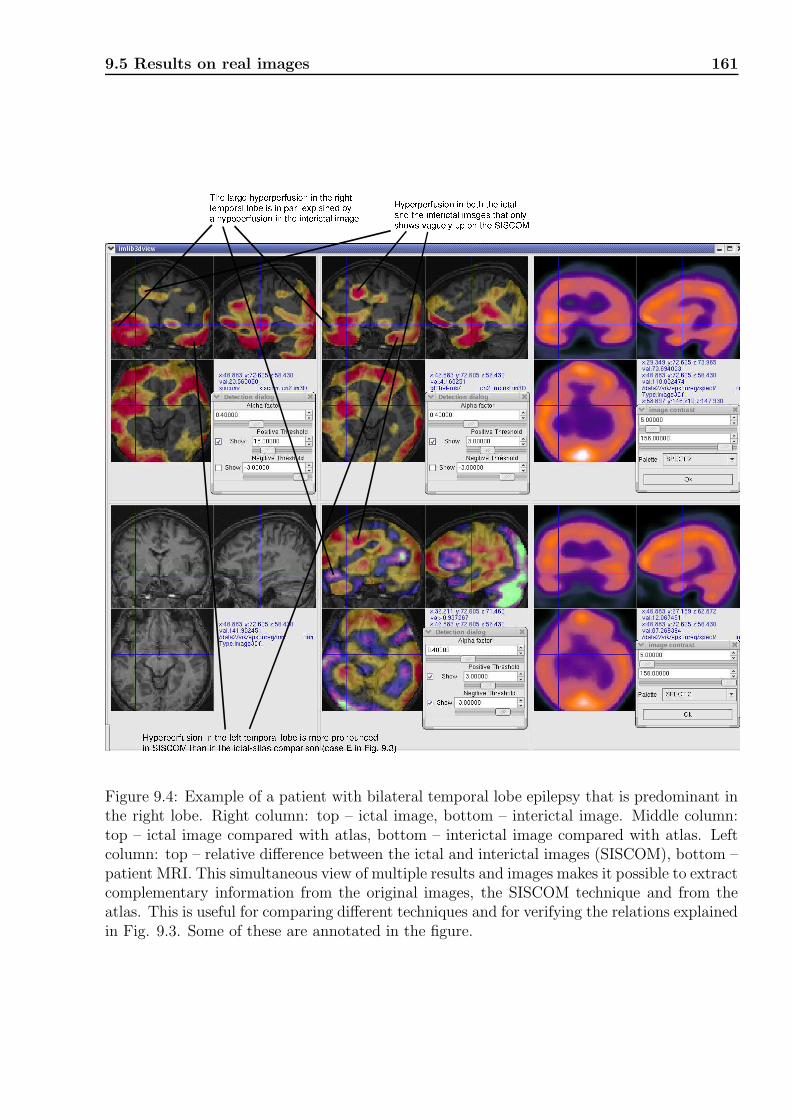
9.5 Results on real images 161
Figure 9.4: Example of a patient with bilateral temporal lobe epilepsy that is predominant inthe right lobe. Right column: top – ictal image, bottom – interictal image. Middle column:top – ictal image compared with atlas, bottom – interictal image compared with atlas. Leftcolumn: top – relative difference between the ictal and interictal images (SISCOM), bottom –patient MRI. This simultaneous view of multiple results and images makes it possible to extractcomplementary information from the original images, the SISCOM technique and from theatlas. This is useful for comparing different techniques and for verifying the relations explainedin Fig. 9.3. Some of these are annotated in the figure.

162 Clinical Application: Epilepsy
Figure 9.5: Another patient in the same kind of display as in Fig. 9.4. Right column: top –ictal image, bottom – interictal image. Middle column: top – ictal image compared with atlas,bottom – interictal image compared with atlas. Left column: top – relative difference betweenthe ictal and interictal images (SISCOM), bottom – patient MRI. The blue cursor is placedon the left hippocampus where a hyperperfusion with respect to the atlas is detected that ispartially explained by a hyperperfusion in the interictal image, and therefore goes undetectedby in the SISCOM image. Note also that this kind of abnormality with respect to normalityis difficult to see directly in the original ictal and interictal images.

9.5 Results on real images 163
Figure 9.6: Examples of significance images of another patient with bilateral temporal lobeepilepsy. Top-left: ictal image compared voxel-by-voxel to the atlas (local model). Top-right:ictal image compared to the atlas (global model, PCA3). Bottom-left: ictal image compared tothe atlas (robust global model, PCA3). Bottom-right: difference of ictal and interictal images(SISCOM). Generally, we see that SISCOM yields a much smoother significance image (brightfor hyper perfusion and dark for hypoperfusion) than the atlas methods. The atlas methodsshow more focused abnormalities than the SISCOM image. As in this example, the localsignificance images are in general smoother than the global significance images. However, atthe position of the cursor (cross), the global models signal more significant abnormality thanthe local model. Between the global methods there is only a small difference, shown in thedifference image Fig. 9.7.

164 Clinical Application: Epilepsy
Figure 9.7: Difference between the significance image obtained by the robust global model(bottom-left) and the global model (top-right) in Fig. 9.6 using the same display contrast.This is the image where we observed the largest difference between these models, ranging from-4.1 to 2.6.
9.5.3 Affine versus deformable registration
In Fig. 9.8 is shown an example of an ictal-atlas comparison using an affine transformationmodel and a deformable deformation model for image registration (see also Sec. 7.3, p. 120).Even though the results often bear resemblance, there are some differences when using thesetwo approaches. In this example, an important spot of hyperperfusion was not detected (oronly weakly detected) when using the affine registration scheme instead of the deformablescheme. We have also observed that the path of discharge is quite differently depicted in theictal-atlas (affine) comparison as to the SISCOM image, whereas the ictal-atlas (deformable)comparison is quite similar. We also know from the evaluation study in Ch. 8 that the atlasthat has been constructed using the deformable registration scheme is more reliable.
9.6 Conclusion and future work
In this chapter we have presented some preliminary results on real images of patients withepilepsy. These illustrate some of the potentials that the use of an atlas have for aiding thediagnosis. In particular, the type of detection observed around the hippocampus in Fig. 9.5seems to be of much interest to the medical expert. The application to images of epilepsywas chosen because the atlasing method can be compared to the existing SISCOM technique.However, its application is of more importance in other pathologies where no reference imagesare available and no other quantitative method exists.
In order to fully validate our approach, further systematic studies must be conducted. Forthis, we are planning a systematic study of the database of treated epilepsy patients that isaccessible at the institute. As we have observed in the experimental studies of 2-D images (Ch.5), we think the atlas will profit more from a larger database of normal subjects (the atlasthat was used for these preliminary results contained only 20 images) so that the descriptionof variations of normal perfusion is improved.
The medical experts show great interest in our atlasing system, not only for the applicationin epilepsy, but also for other pathologies. However, there is still some work to be done beforea medical expert can use the system without any technical assistance. In the meantime, weprovide a temporary solution where some functionality is made accessible through trainingand assistance.
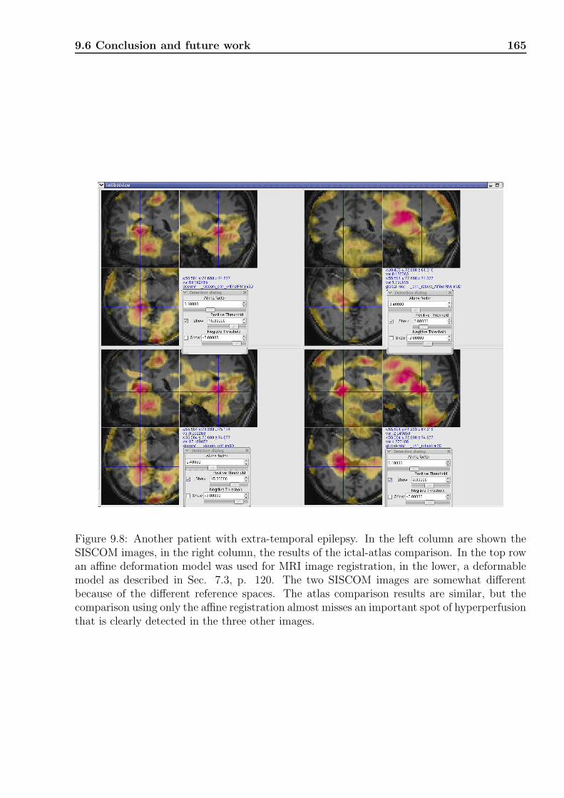
9.6 Conclusion and future work 165
Figure 9.8: Another patient with extra-temporal epilepsy. In the left column are shown theSISCOM images, in the right column, the results of the ictal-atlas comparison. In the top rowan affine deformation model was used for MRI image registration, in the lower, a deformablemodel as described in Sec. 7.3, p. 120. The two SISCOM images are somewhat differentbecause of the different reference spaces. The atlas comparison results are similar, but thecomparison using only the affine registration almost misses an important spot of hyperperfusionthat is clearly detected in the three other images.

166 Clinical Application: Epilepsy
Figure 9.9: The same comparison as in Fig. 9.8 for another patient with right temporal lobeepilepsy. In the left column are shown the SISCOM images, in the right column, the resultsof the ictal-atlas comparison. In the top row an affine deformation model was used for MRIimage registration, in the lower, a deformable model as described in Sec. 7.3, p. 120. Twobilateral paths that are clearly depicted in the SISCOM images, deviates in the affine atlascomparison, whereas the deformable atlas comparison accentuates these. Both atlases alsoshow small regions of hyperperfusion in the temporal lobes (the deformable somewhat morethan the affine) that are almost inexistent in the SISCOM images. In a second ictal scan ofthis patient, a strong hyperperfusion was found in the right temporal lobe with small spreadto the contralateral temporal lobe and strong spread to the frontal and superior parts of thebrain.

Chapter 10
Conclusions and future work
In this final chapter, we summarize this thesis and its contributions. To conclude, some ideasfor future work are presented.
10.1 Summary and discussion
This thesis and the contributions of this thesis are divided into two parts. One concerns thetheoretical developments of a new probabilistic model. The second concerns the creation andevaluation of an atlas of brain perfusion.
We began Part II by studying different appearance-based models used in computer vision.In particular, we studied in detail global, linear models that rely on PCA for dimensionreduction. These have been applied with much success in the modeling of images of bothobjects and faces. In Sec. 3.3.5, p. 39, we established the relationship between the popularmodel of Moghaddam and Pentland [162] and the theoretical development of the PPCA modelby Tipping and Bishop [211]. Even though the applications (face recognition and computervision) for these models are far from our problem of creating an atlas of brain perfusion, theyare attractive to us because (1) of their success, (2) of their simplicity, and (3) they are learningmethods.
In Ch. 4, we then presented an original, non-Gaussian appearance model for unsupervisedlearning. The model is based on a linear factor analysis model, but has a non-Gaussiansubspace distribution and a non-Gaussian (robust) noise distribution. The first importantproblem to solve for any such model is the reconstruction problem (also called the inferenceproblem), which was defined in Sec. 4.1.1, p. 61. We solved this problem by developingthe robust modified mean shift algorithm, [220]. The algorithm is based on half-quadratictheory and an extension of the mean shift procedure. In experiments performed on a standardcomputer vision database, we showed this model’s superiority to other well known models.These experiments also permitted us to better understand the behavior of our approach indifferent situations. In particular, in Sec. 5.4.2, p. 84 we drew the conclusion that for the modelto be effective, it must be “sufficiently accurate”. This is in general obtained by using enoughtraining images, and a sufficient number of eigenvectors. This gain must be compared to theincreased computational cost of the model. Indeed, depending on the application, one mustclarify whether robust modeling is indeed necessary. Our model is particularly well adapted todifficult situations with much image degradation as the experiments show. Another difficultymight arise from the multimodal nature of the posterior density function which makes it only

168 Conclusions and future work
possible to guarantee that the algorithm can find local minima. In some situations it mighttherefore be necessary to use multiple initializations in order to find a satisfactory solution.Finally, note that this model is not limited to the modeling of images. It is indeed formulatedin a very general manner and could be applied to pattern recognition problems in general.This opens for many interesting perspectives for future work.
In Part III, we returned to the problem of creating an atlas of brain perfusion that origi-nated this work. We began this part with a comprehensive study of statistical models used tocreate atlases of functional brain images both for research and in a clinical setting. Presentingthese in a unified way is difficult because of the many different applications (image modalities,pathologies, study designs) and the many possible ways of preprocessing the images beforestatistical modeling. This is further complicated by the rich statistical and medical nomen-clature. Nevertheless, we proposed a review where the methods were classified based on (1)whether the statistical models used are multivariate or univariate in nature, and (2) whatfeature is modeled. To our knowledge, no such review exist in the literature.
We take particular notice that Houston et al. [104] independently developed a model thatis very similar to the classical linear PCA-based appearance models used in computer vision.They also found a clever way of making localized detections for this kind of global models.This method is important since otherwise only a global statement about an image into a class(pathology or not) would be possible. This local detection is simply done by weighting theresidual obtained from the image reconstruction problem by the non-isotropic variance of thelearning base images. We formalized this model and situated it with respect to the modelspresented in Ch. 4.
In Ch. 6 we continued by presenting different techniques for SPECT and MRI imageprocessing: registration, brain segmentation and intensity normalization. We presented themain characteristics of the algorithms for deformable, inter-subject, MRI-MRI registrationand for rigid, intra-subject, SPECT-MRI registration that have been developed prior to, andduring this work by other researchers at our laboratory. These could therefore in Sec. 7.3,p. 120 be used to develop a registration scheme that is specifically adapted to our needs ofregistering SPECT images of multiple subjects for the creation of an atlas. This scheme hasthe particularities that deformable registration was used (generally, only affine or piecewiseaffine is used), and that a step of transformation field filtering was introduced. Deformableregistration is still a domain of intense research that is still far from being solved. The schemethat we propose seems to be the best possible with respect to atlas creation (and with thetechniques to which we have access). However, we believe there is still margin of possibleimprovement concerning inter-subject registration.
In Sec. 7.5, p. 126, an obvious extension to the standard linear regression solution forjoint histogram intensity normalization was proposed. Total least squares was used to modelerrors in both images as opposed to standard linear regression where only the source (and notthe reference) image is considered to contain errors. We have not yet performed systematiccomparison between the LS and the TLS normalization. We only argument for the TLS methodwith theoretical arguments. Such comparison is indeed difficult as the intensity normalizationissue is associated with much uncertainty and dispute. One possible study would however beto evaluate the robustness of the different registration schemes using our evaluation scheme(Ch. 8).
In Ch. 8, we presented an original and comprehensive evaluation study that was used tocompare and evaluate several important aspects concerning atlas creation: statistical models,

10.2 Future work 169
heterogeneity of detection across different regions in the brain, registration schemes and finallyintensity normalization. The results were described in Sec. 8.6, p. 143, see also [219, 221].The evaluation study aims at making statements about the validity of assumptions underlyingthe statistical models and about the sensitivity of the model at detecting abnormalities. Thishas not been done before.
Finally, in Ch. 9, we have shown some preliminary results using the atlas to aid theinterpretation of images of patients with epilepsy. The results showed good coherence withthe results obtained by the more usual SISCOM technique, but also some differences. Thesetwo techniques seem to yield complementary information about resting state brain perfusionand changes therein induced by epileptic seizures. However, further analyses and tests mustbe performed. In a first time, the atlas will serve the clinician as a supplemental tool withlimited confidence level.
Several software libraries were developed and co-developed during this thesis. The librarieswere developed using advanced features of the C++ programming language (generic program-ming by means of templates, [218], object-oriented design) and modern software engineeringtechniques (design patterns [75], unit tests1). In particular, the author contributed to the opensource, software package ImLib3D 2 which was designed and conceptualized by M. Bosc. Thiswork gave rise to a conference publication [19]. Finally, the libraries have been implementedas a module of the in-house, proprietary software Medimax through which the probabilisticatlas is accessible to physicians and researchers at IPB (Institut Physique Biologique).
A weakness of this thesis is that we have not explicitly modeled sources of variation thatstem from the image acquisition process, nor have we explored/evaluated the intra-individualvariation and dependance on age and gender. The contribution of these error sources to thetotal image variation need to be better understood. Since we have a database with two imagesof each subject, this latter kind of variation would be possible to study.
10.2 Future work
Every thesis tries to shed some light on a specific problem. The contributions of this thesishave been summarized above. However, it seems to the author of this document that thenumber of resolved questions remains largely inferior to the number of unresolved questions towhich this work gives rise. This is no burden – rather an opportunity. However, only a limitednumber of problems should be attacked at a time, and it is probably wise to choose those thatare the most promising. Paths for future investigation can be divided into (1) those concerningour original model, both at the theoretical and practical level, and (2) those concerning theapplication of the atlas to routine clinical examinations and medical research.
10.2.1 Model
Some paths for future work concerning our original model were already detailed in Sec. 4.8,p. 70. These are summarized and some are added.
1http://www.extremeprogramming.org/2http://imlib3d.sourceforge.net

170 Conclusions and future work
Theoretical
The most interesting problem to solve from a theoretical viewpoint is of course the systemidentification (or model estimation) problem for our model. We see a possibility for thisby means of the EM-algorithm as mentioned in Sec. 4.8. If we succeed in this, we wouldindeed have a full-blown method for unsupervised dimension reduction with possibly manyapplications in perspective. Furthermore, it would be desirable to derive a convergence proofof the RMMS algorithm. Also, a better understanding of the convergence properties of thisalgorithm is necessary.
Generalized linear models are often mentioned in the context of global linear models. Itwould be interesting to investigate whether it is possible to derive a generalized modified meanshift for such models. Finally, there are several links to be established to recent probabilisticmodels. Palmer [182, 181] for example shows that there are links between half-quadratic theoryand ICA. Saul and Roweis [191] have recently proposed a mixture model of local linear modelswith a new learning concept that bears similarities to our model.
Practical
There is a need to continue experimentation with multiple initialization and marginal proba-bility for detection. We showed in Sec. 4.8 how one can calculate the marginal probability ofthe non-occluded part of the image. This makes it possible to use multiple initializations forthe RMMS algorithm. This could solve the problem where the robust algorithm sometimesfails with a large margin as observed in our experiments.
10.2.2 Atlas, model
As we have found during the experiments in Ch. 5 and in the pilot study briefly mentionedin Sec. 8.6.1, p. 145 (Fig. 8.7, p. 146), the performance of the models we have developedincreases with more model accuracy. A more accurate model is obtained with a larger (andtherefore more representative) database of normal images and with more eigenvectors in themodel. This is therefore important work to do in the near future. Currently the atlas isconstructed from 20 subjects. Another ten images of normal subjects have recently beenacquired and will therefore be included in the atlas shortly. However, a total of 30 images isprobably still not sufficient. This number should probably be in the hundreds. Because of theexpenses of acquisition, it is important that image centers share images. Comparing imagesthat come from different gamma cameras may however pose problems. In this case, inter-center image variability should be modeled, or alternatively, adapted normalization (spatialand intensity) procedures should be developed.
Modeling global activity, age, gender and handedness
An aspect that distinguishes the atlas application from a typical computer vision applicationis that we possess additional knowledge such as age, gender and handedness of the subjects.Since these are factors that are known to influence normal blood flow [127], these shouldbe included in the model. This necessitates however, even more reference images. From amathematical viewpoint, this extension is straightforward and is shown for the modeling ofglobal activity. The extension to age, gender and handedness follows the same scheme.
Instead of considering the intensity normalization as a separate preprocessing step beforemodeling, an alternative would be to take the global activity into account in the model as in

10.2 Future work 171
the SPM ANCOVA model, Sec. 6.6.4, p. 116. This can be done by considering the followingMANCOVA model3 for scan j:
yj = Wxj + µ + ξ(gj − g·) + εj (10.1)
The model is the same as the global linear model in Eq. 4.1, p. 60, with an additional D-dimensional constant ξ, the global activity in image j, gj, and the average global activity inthe learning base images, g·.
Under this model and for Gaussian isotropic noise we have that:
p(yj|µ, ξ) = N (µ + ξ(gj − g·), σ2I + WW T )
From this, we can derive the maximum likelihood estimators of ξ and µ as
ξ =
∑
j(gj − g·)yj∑
j(gj − g·)2
and
µ =1
J
∑
j
(
yj − ξ(gj − g·))
.
Note, that the mean, µ, now is the mean of the intensity-corrected data. Least squaresprojection is done as usual
xj = (W T W )−1W T (yj − µ)
whether j is an image of the learning base or not. On the mean- and global activity-free data,PCA can now be performed as usual. In this MANCOVA model, ξ corrects for global intensitychanges by adding a proportion of the global intensity difference of an image to each voxelintensity. Since it is estimated, we therefore lose one degree of freedom when estimating thevoxel variance estimation (see Eq. 6.1, p. 100).
Multi-modal, integrated and disease-specific atlases
For future work, we think that incorporating more sources of variability in the probabilisticatlas model will be necessary. Conjointly modeling different image modalities, image acqui-sition, image reconstruction and image processing (registration, intensity normalization andsegmentation) could benefit the task of interpreting and analyzing these images. The im-age reconstruction and processing tools that today work indepently of each other, could alsomutually improve from such modeling. Likewise, it may also be necessary to develop disease-specific atlases in order to improve the utility and performance of quantitative, computer aideddiagnosis.
10.2.3 Atlas, application
It is desirable to evaluate the influence of the atlas in a clinical setting. For this, we envisagea retrospective study of epilepsy patients that have undergone surgery. For these patients,there is a well established ground truth that could be used as a reference. However, sincethe differences in models are small, very large cohorts are necessary to show any significant
3A MANCOVA model was also proposed by Friston et al. [70]. However, this model is different in that thedimensionality of the data is reduced before global intensity changes and age are modeled.

172 Conclusions and future work
difference. Furthermore, we are in the planning stage of a study of patients with migraine.The hypothesis here is that a situation of “aura” that certain patients experience before themigraine, is explained by an increased activity in the brain stem. An injection would thereforebe made at the moment these patients experience this aura to measure the blood flow at thismoment.

Part IV
Appendix


Appendix A
Modified Mean Shift
In this chapter we have collected the calculations that were left out from the derivation of themodified mean shift in the main text (Ch. 4). We first show how to calculate the MAP kernelestimate from which we obtain the more “interpretable” form of the modified mean shift (Eq.4.33, p. 69):
mms(x) =
[∑Jj=1 cjΓj(x)µj∑J
j=1 cjΓj(x)− x
]
. (A.1)
We then proceed to describe how to obtain the simplified Modified Mean Shift term of Eq.4.34, p. 69. This is first done by simplifying/rewriting Eq. A.1, then an alternative approach isderived. Finally, in Sec. A.3, we bring the convergence proof for the modified mean shift. Notethat we have not derived a convergence proof for robust modified mean shift optimization.
A.1 Modified Kernel Estimate
We shall show how to obtain the posterior density (Eq. 4.25, p. 68):
p(x|y) = c1
J
J∑
j=1
cjΓj(x), (A.2)
which we denote the posterior kernel estimate, from (Eq. 4.24, p. 68)
p(x|y) =1
p(y)
1
J
J∑
j=1
p(y|x)pj(x). (A.3)
The calculations are not complicated, but a bit tedious. Intuitively, we see that since each ofthe two factors of the product p(y|x)pj(x) are Gaussians, the product itself is also Gaussian.We therefore only have to find the quadratic form of the exponential of this product. FromEq. A.3 we have
p(y|x)pj(x) = k1k2 exp(−1
2
[(y −Wx)TΣ−1
ε (y −Wx) + (x− xj)TΣ−1
x (x− xj)]), (A.4)
where k1 and k2 are constants. Since there are only quadratic terms in the brackets of thisexponential, we can introduce a mean, µj, and a symmetric covariance matrix, Σ, so that
(x− µj)TΣ−1(x− µj) = xTΣ−1x− 2µT
j Σ−1x + µTj Σ−1µj. (A.5)

176 Modified Mean Shift
Writing out the brackets of Eq. A.4 yields
xT (W TΣ−1ε W + Σ−1
x )x− 2(yTΣ−1ε W + xT
j Σ−1x )x + yTΣ−1
ε y + xTj Σ−1
x xj (A.6)
and by comparing terms with Eq. A.5 we directly obtain
Σ−1 = W TΣ−1ε W + Σ−1
x , (A.7)
which yields (4.26) (Note that Σ actually is symmetric as Σε and Σx are both symmetric).Furthermore, we have (by comparing terms in Eqs. A.6 and A.5)
µTj Σ−1 = yTΣ−1
ε W + xTj Σ−1
x . (A.8)
By taking the transposeΣ−1µj = W TΣ−1
ε y + Σ−1x xj (A.9)
and multiplicate from the left with Σ, we obtain (4.27).It now remains to calculate the weighting coefficients cj. With Eqs. A.7 and A.8, A.6
becomes(x− µj)
TΣ−1(x− µj)︸ ︷︷ ︸
∝− log(Γj)
−µTj Σ−1µj + xT
j Σ−1x xj + yTΣ−1
ε y︸ ︷︷ ︸
constant−2 log cj
. (A.10)
In this equation only terms depending on j are needed to calculate cj, leaving only the twomiddle terms. All constant terms can flow into the global normalization constant c in Eq.4.25, which is more conveniently determined by integration (Eq. 4.31, p. 68).
As above, we introduce two constants, the symmetrical matrix Ψ and µx, we rewrite thetwo terms in the middle of Eq. A.10 on the quadratic form (the same as Eq. 4.28)
(xj − µx)TΨ−1(xj − µx) = xT
j Ψ−1xj − 2µTx Ψ−1xj + µT
x Ψ−1µx, (A.11)
and compare terms. For this, we need the expression µTj Σ−1µj (from Eq. A.8)
µTj Σ−1µj = (yTΣ−1
ε W + xTj Σ−1
x )Σ(W TΣ−1ε y + Σ−1
x xj) (A.12)
= yTΣ−1ε WΣW T Σ−1
ε y + 2yTΣ−1ε WΣΣ−1
x xj + xTj Σ−1
x ΣΣ−1x xj, (A.13)
with which, the last three terms in Eq. A.10 becomes
yTΣ−1ε (I −WΣW TΣ−1
ε )y − 2yTΣ−1ε WΣΣ−1
x xj + xTj Σ−1
x (I −ΣΣ−1x )xj. (A.14)
Comparing with Eq. A.11 and only considering terms depending on j, yields
Ψ−1 = Σ−1x (I −ΣΣ−1
x ), (A.15)
or equivalentlyΨ = (I −ΣΣ−1
x )−1Σx (A.16)
which is the same expression as Eq. 4.29 For µx we have
µTx Ψ−1 = yTΣ−1
ε WΣΣ−1x (A.17)
from which Eq. 4.30 follows. Finally, in Eq. A.11, we assumed that Ψ was symmetric. Thisis verified as follows:
ΨT = Σx(I −Σ−1x Σ)−1
= (Σ−1x )−1(I −Σ−1
x Σ)−1
= ((I −Σ−1x Σ)Σ−1
x )−1
= (Σ−1x (I −ΣΣ−1
x ))−1
= (I −ΣΣ−1x )−1Σx
= Ψ.
(A.18)
A.2 Simplified Modified Mean Shift 177
A.2 Simplified Modified Mean Shift
We can obtain an expression for the modified mean shift mms(x) that is computationally lessexpensive than the expression in Eq. A.1, and that is based on the standard mean shift term.For this we need to rewrite the expression cjΓj(·) in Eq. A.1, so that we only keep all that isdependent on j. The rest can be eliminated from the fraction. We begin by writing
cjΓj(x) = exp
(
−1
2
[(xj − µx)
TΨ−1(xj − µx) + (x− µj)TΣ−1(x− µj)
])
. (A.19)
Writing out the exponent yields the expression
xTj Ψ−1xj − 2µT
x Ψ−1xj + µTx Ψ−1µx + xTΣ−1x− 2xTΣ−1µj + µT
j Σ−1µj (A.20)
from which we keep only the terms depending on j. Thus, substituting for µj (from Eqs. A.8and A.12) and leaving out the terms dependent on x, yields
xTj (Ψ−1 + Σ−1
x ΣΣ−1x )xj + 2(yTΣ−1
ε WΣΣ−1x − xTΣ−1
x − µTx Ψ−1)xj, (A.21)
which, with Eqs. A.15 and A.17, simplifies to
xTj Σ−1
x xj − 2xTΣ−1x xj. (A.22)
We thus finally obtain
cjΓj(x) ∝ Θj(x) = exp(−1
2(x− xj)
TΣ−1x (x− xj)). (A.23)
With Θj(·) and µj, we can now rewrite the mms(x) expression in Eq. A.1 as
mms(x) =
∑Jj=1 Θj(x)µj∑J
j=1 Θj(x)− x
=
∑Jj=1 Θj(x)ΣW TΣ−1
ε y +∑J
j=1 Θj(x)ΣΣ−1x xj
∑Jj=1 Θj(x)
− x
= Σ
(
W TΣ−1ε y + Σ−1
x
∑Jj=1 Θj(x)xj∑J
j=1 Θj(x)
)
− x
, (A.24)
which is the same as Eq. 4.34, p. 69.
A.2.1 An alternative way of obtaining the simplified modified mean
shift
The modified mean shift and the simplified version of the Modified Mean Shift can be obtainedby rewriting the posterior probability Eq. A.3 into Eq. A.2, differentiating and eliminatingterms from the quotient. An alternative way of obtaining the same expression as (A.24), is byderiving the composite posterior probability (A.3)
arg maxx
p(x|y) = arg maxx
p(y|x)p(x)
p(y)= arg max
xp(y|x)p(x), (A.25)

178 Modified Mean Shift
directly to find ∇p(y|x)p(x).
With
∇pj(x) = pj(x)Σx−1(x− xj) (A.26)
and
∇p(y|x) = −p(y|x)W TΣε−1(y −Wx) (A.27)
we have
∇p(y|x)p(x) = p(x)∇p(y|x) + p(y|x)∇p(x)
= p(y|x)p(x)W TΣε−1(y −Wx)− p(y|x)
1
J
J∑
j=1
pj(x)Σx−1(x− xj)
= p(y|x)
p(x)W TΣε−1(y −Wx) + Σx
−1
[
1
J
J∑
j=1
pj(x)
]
︸ ︷︷ ︸
p(x)
[∑Jj=1 pj(x)xj∑J
j=1 pj(x)− x
]
= p(y|x)p(x)
W TΣε−1y + Σx
−1
∑Jj=1 pj(x)xj∑J
j=1 pj(x)− (W TΣε
−1W + Σx−1)
︸ ︷︷ ︸
Σ−1
x
= p(y|x)p(x)Σ−1
[
Σ
(
W TΣε−1y + Σx
−1
∑Jj=1 pj(x)xj∑J
j=1 pj(x)
)
− x
]
,
(A.28)
which is the same as Eq. 4.34, p. 69.
A.3 Convergence Proof of the Modified Mean Shift
With the modified mean shift expression in Eq. A.1, the convergence of an optimizationalgorithm based on the modified mean shift can be proved in an analog manner to the originalmean shift convergence proof [40]1. In the following, we make use of the following notationsand relations:
• The iteration index, i.
• The positive definite quadratic form:
qj(x) = (x− µj)TΣ−1(x− µj),
where Σ is a non-singular, symmetric matrix with positive eigenvalues.
• The (normal) kernel:
k(x) = exp(−1
2x).
1This is actually the main advantage of Eq. A.1 over the simplified modified mean shift expression, Eq.A.28.

A.3 Convergence Proof of the Modified Mean Shift 179
Since this kernel is convex, and since k′(x) = −12k(x), the following relation holds:
k(x2)− k(x1) ≥1
2k(x1)(x1 − x2), (A.29)
for x1 6= x2 and x1, x2 ≥ 0.
• The updated subspace variable estimate is then given by (rewriting Eq. A.1):
xi+1 =
∑Jj=1 cjk(qj(xi))µj∑J
j=1 cjk(qj(xi))= mms(xi) + xi, (A.30)
which yields a sequence of posterior probabilities, p(xi|y)i=1,2....
We can now prove the following theorem:
Theorem 1 With the normal kernel, k(x), the sequences xii=1,2... and p(xi|y)i=1,2... con-verge, and p(xi|y)i=1,2... is monotonically increasing.
Proof
Since J is finite, the sequence p(xi|y)i=1,2... is bounded (recall p(x|y) from Eq. A.2). Itis therefore sufficient to show that p(xi|y)i=1,2... is strictly monotonic increasing, i.e. ifxi 6= xi+1, then
p(xi|y) < p(xi+1|y), i = 1, 2 . . . .
From Eq. A.2, using the above notation, we have
p(xi+1|y)− p(xi|y) =c
J
J∑
j=1
cj[k(qj(xi+1))− k(qj(xi))
]. (A.31)
With Eq. A.29, we can rewrite this into
p(xi+1|y)− p(xi|y) ≥ c
2J
J∑
j=1
cjk(qj(xi))[qj(xi)− qj(xi+1)
]
=c
2J
J∑
j=1
cjk(qj(xi))[xT
i Σ−1xi − 2xTi Σ−1µj − xT
i+1Σ−1xi+1 + 2xT
i+1Σ−1µj
],
which with Eq. A.30 becomes,
p(xi+1|y)− p(xi|y) ≥ c
2J[xT
i Σ−1xi − 2xTi Σ−1xi+1 − xT
i+1Σ−1xi+1+
+2xTi+1Σ
−1xi+1] ·J∑
j=1
cjk(qj(xi))
=c
2J(xi+1 − xi)
TΣ−1(xi+1 − xi)︸ ︷︷ ︸
≥0
J∑
j=1
cjk(qj(xi))
︸ ︷︷ ︸
>0
.
(A.32)

180 Modified Mean Shift
With the last product being strictly positive (recall that xi 6= xi+1 and Σ positive definite),we have that the sequence p(xi|y)i=1,2... is monotonically increasing.
To show the convergence in the euclidean space of the sequence xii=1,2..., it is sufficientto show that ||xi+m − xi||2 is bounded for m → ∞. Summing successive iterations from Eq.A.32 yields:
p(xi+m|y)− p(xi|y) ≥ c
2J(xi+m − xi+m−1)
TΣ−1(xi+m − xi+m−1)J∑
j=1
cjk(qj(xi+m−1)) + . . .
+c
2J(xi+1 − xi)
TΣ−1(xi+1 − xi)J∑
j=1
cjk(qj(xi))
≥ c
2J
[(xi+m − xi+m−1)
TΣ−1(xi+m − xi+m−1) + . . .
+c
2J(xi+1 − xi)
TΣ−1(xi+1 − xi)]M
≥ c
2J(xi+m − xi)
TΣ−1(xi+m − xi)M,
where M is the the minimum (always strictly positive) of the sum∑J
j=1 cjk(qj(xi)) for all
xii=1,2.... Since p(xi|y)i=1,2... is convergent, it follows that (xi+m − xi)TΣ−1(xi+m − xi)
is bounded. In particular, we have that for Σ = I, the euclidean distance, ||xi+m − xi||2, isbounded.

Appendix B
Small sample size and covariancematrix decomposition
How to calculate the principal components, or equivalently approximating the covariance ma-trix of high dimensional random variables, is repeatedly described in journal papers despitethe fact that it has been known for quite some time. Fukunaga already described how to dothis 14 years ago [72]. We recall this description and show that this method is actually thesingular value decomposition of the sample matrix (which is today the more usual way to go).
From J observations, yj, we estimate the mean and the covariance matrix of the randomvector y
µ =1
J
J∑
j
yj, Σ =1
J − 1
J∑
j
(yj − µ)(yj − µ)T .
Since Σ is a function of J or less linearly independent vectors, its rank can only be J or less.Furthermore, because of the estimated mean vector µ we “loose” a degree of freedom and themaximum possible rank is (J − 1). If J < D, where D is the dimension of the observationspace, Σ is singular. Furthermore, since the covariance matrix is of the size D×D it becomescomputationally unhandly, if not untractable for large D (D >> J).
Some carefulness is therefore necessary to solve the eigenproblem. Fukunaga [72] proposesto invert the roles of variables and samples. Let Y = [y1 . . .yJ ] be the sample matrix and Y
the mean free sample matrix. Then we can write Σ = 1J−1
Y YT. Instead of using Σ, we can
calculate the eigenvectors, vq, and eigenvalues, λj, of 1J−1
YTY , which is only J × J
1
J − 1(Y
TY )V = V Λ = [v1 . . .vJ ]
λ1 0. . .
0 λJ−1
,
where V is the matrix of eigenvectors. Multiplying from the left with Y yields
1
J − 1(Y Y
T)(Y V ) = (Y V )Λ.
Thus, (Y V ) and Λ are the (J − 1) eigenvectors and eigenvalues of Σ. The other (D− J + 1)eigenvalues are all zero and their eigenvectors are indefinite.

182 Small sample size and covariance matrix decomposition
The matrix (Y V ) represents orthogonal vectors. To obtain orthonormal ones, we have todivide each column vector of (Y V ) by ((J − 1)λj)
1/2 yielding:
U =1√J − 1
Y V Λ−1/2. (B.1)
We can validate this as follows:
UT U =1
J − 1Λ−1/2V T Y
TY V Λ−1/2 = Λ−1/2V T V ΛΛ−1/2 = I.
Rewriting Eq. B.1, we can express Y as
1√J − 1
Y = UΛ1/2V T
which is exactly the SVD of 1√J−1
Y (or more precisely what Golub et al. call thin SVD)
[82]. We have found that the SVD algorithm, based on the one-sided Jacobi orthogonalization([74]), gives the most precise results.
Appendix C
Peer-reviewed publications by theauthor
International journals
T. Vik, F. Heitz, and J.-P. Armspach. On the modeling, construction and evaluation of aprobabilistic atlas of brain perfusion. NeuroImage, 2004, 14 pages, accepted for publication.
International conferences with proceedings
T. Vik, F. Heitz, and J.-P. Armspach. Statistical atlas-based detection of abnormalities inbrain perfusion: Comparing models and estimating detection performance. In R. E. Ellisand T. M. Peters, editors, Int. Conf. on Medical Image Computing & Computer AssistedIntervention 2003, Lecture Notes in Computer Science 2879, pages 838-845, Toronto, Canada,November 2003.
M. Bosc, T. Vik, J.-P. Armspach, and F. Heitz. ImLib3D: An efficient, open source,medical image processing framework in C++. In R. E. Ellis and T. M. Peters, editors, Int.Conf. on Medical Image Computing & Computer Assisted Intervention 2003, Lecture Notesin Computer Science 2879, pages 981-982, Toronto, Canada, November 2003.
T. Vik, F. Heitz, and P. Charbonnier. Mean shift-based bayesian image reconstructioninto visual subspace. In Proceedings of the 2003 International Conference on Image Processing(ICIP 2003), Barcelona, Spain, September 2003.

184 Peer-reviewed publications by the author

Bibliography
[1] P. Acton and K. Friston. Statistical parametric mapping in functional neuroimaging:beyond PET and fMRI activation studies. European Journal of Nuclear Medicine,25(7):663–667, July 1998. Editorial.
[2] D. G. Amen. Images Into Human Behavior: A Brain SPECT Atlas. Mindworks Press,nd. http://www.brainplace.com/bp/atlas/default.asp.
[3] D. G. Amen, J. C. Wu, and B. Carmichael. The clinical use of brain SPECT imagingin neuropsychiatry. Alasbimn Journal, 5(19), January 2003.
[4] T.W. Anderson. An Introduction to Multivariate Statistical Analysis. John Wiley &Sons, 1984.
[5] P. Bartenstein, S. Minoshima, C. Hirsch, K. Buch, F. Willoch, D. Mosch, D. Schad,M. Schwaiger, and A. Kurz. Quantitative assessment of cerebral blood flow in patientswith Alzheimer’s disease by SPECT. The Journal of Nuclear Medicine, 38(7):1095–1101,July 1997.
[6] M. S. Bartlett, J. R. Movellan, and T. J. Sejnowski. Face recognition by independentcomponent analysis. IEEE Trans. Neural Networks, 13:1450–1464, 2002.
[7] C. F. Beckmann and S. Smith. Probabilistic independent component analysis for func-tional magnetic resonance imaging. IEEE Trans. Med. Imag., 23(2):137–152, February2004.
[8] P. N. Belhumeur, J. P. Hespanha, and D. J. Kriegman. Eigenfaces vs. Fisherfaces:Recognition using class specific linear projection. IEEE Trans. Pattern Anal. MachineIntell., 19(7):711–720, July 1997.
[9] P. N. Belhumeur and D. J. Kriegman. What is the set of images of an object under allpossible illumination conditions. International Journal of Computer Vision, 28(3):245–260, March 1998.
[10] H. Benali, I. Buvat, F. Frouin, J. P. Bazin, and R. Di Paola. A statistical model forthe determination of the optimal metric in factor analysis of medical image sequences(FAMIS). Phys. Med. Biol., 38:1065–1080, 1993.
[11] C. Bishop and M. Tipping. A hierarchical latent variable model for data visualization.IEEE Trans. Pattern Anal. Machine Intell., 20(3):281–293, 1998.
[12] C. M. Bishop. Neural Networks for Pattern Recognition. Oxford University Press, 1995.

186 BIBLIOGRAPHY
[13] M. J. Black and A. D. Jepson. EigenTracking: Robust matching and tracking of ar-ticulated objects using a view-based representation. International Journal of ComputerVision, 26(1):63–84, 1998.
[14] M. J. Black and A. Rangarajan. On the unification of line processes, outlier rejection,and robust statistics with applications in early vision. International Journal of ComputerVision, 19(1):57–91, 1996.
[15] D.A. Boas, D.H. Brooks, E.L. Miller, C.A. DiMarzio, M. Kilmer, and R.J. Gaudette.Imaging the body with diffuse optical tomography. IEEE Signal Processing Magazine,pages 57–75, November 2001.
[16] M. Borga, T. Landelius, and H. Knutsson. A unified approach to PCA, PLS, MLRand CCA. Report LiTH-ISY-R-1992, ISY, Linkoping University, Sweden, SE-581 83Linkoping, Sweden, November 1997.
[17] M. Bosc. Contribution a la detection de changements dans des sequences IRM 3D mul-timodales. PhD thesis, Universite Louis Pasteur I, Strasbourg, 2003.
[18] M. Bosc, F. Heitz, J.-P. Armspach, I. Namer, D. Gounot, and L. Rumbach. Automaticchange detection in multi-modal serial MRI: Application to multiple sclerosis lesionevolution. NeuroImage, 20(2):643–656, October 2003.
[19] M. Bosc, T. Vik, J.-P. Armspach, and F. Heitz. ImLib3D: An efficient, open source,medical image processing framework in C++. In R. E. Ellis and T. M. Peters, editors,MICCAI 2003, LNCS 2879, pages 981–982, November 2003.
[20] P. Bourdieu. La distinction : Critique sociale du jugement. Les Editions de Minuit,1979.
[21] N. Boussion, C. Houzard, K. Ostrowsky, P. Ryvlin, F. Maugiere, and L. Cinotti. Au-tomated detection of local normalization areas for ictal-interictal subtraction brainSPECT. The Journal of Nuclear Medicine, 43:1419–1425, 2002.
[22] N. Boussion, P. Ryvlin, J. Isnard, C. Houzard, F. Maugiere, and L. Cinotti. Towardsan optimal reference region in single photon emission tomography difference images inepilepsy. European Journal of Nuclear Medicine, 27:155–160, 2000.
[23] K. W. Bowyer. Validation of medical image analysis techniques. In M. Sonka and J. M.Fitzpatrick, editors, Handbook of Medical Imaging, volume 2, pages 567–607. SPIE Press,2000.
[24] L. Le Briquer and J. C. Gee. Design of a statistical model of brain shape. In J. S.Duncan and G. R. Gindi, editors, XVth Int. Conf. on Information Processing in MedicalImaging, pages 9–13. Springer-Verlag, Heidelberg, 1997.
[25] P. P. Bruyant. Analytic and iterative reconstruction algorithms in SPECT. The Journalof Nuclear Medicine, 43(10):1343–1358, October 2002.
[26] I. Buvat. Toward a standardization of the description and validation of monte carlosimulation codes in spect and pet. The Journal of Nuclear Medicine, 43:207P, 2002.

BIBLIOGRAPHY 187
[27] A. Cachia, J.-F. Mangin, D. Riviere, F. Kherif, N. Boddaert, A. Andrade,D. Papadopoulos-Orfanos, J.-B. Poline, I. Bloch, M. Zilbovicius, P. Sonigo, F. Brunelle,and J. Regis. A primal sketch of the cortex mean curvature: a morphogenesis basedapproach to study the variability of the folding patterns. IEEE Trans. Med. Imag.,22(6):754–765, 2003.
[28] R. Cappelli, D. Maio, and D. Maltoni. Multispace KL for pattern representation andclassification. IEEE Trans. Pattern Anal. Machine Intell., 23(9), September 2001.
[29] M. Carbon, M. Ghilardi, A. Feigin, M. Fukuda, G. Silvestri, M. Mentis, C. Ghez,J. Moeller, and D. Eidelberg. Learning networks in health and Parkinsons’s disease:Reproducibility and treatment effects. Human Brain Mapping, 11:197–211, 2003.
[30] M. Carreira-Perpinan. A review of dimension reduction techniques. Technical report,Dept. of Computer Science, University of Sheffield, January 1997.
[31] B. Chalmond and S. C. Girard. Nonlinear modeling of scattered multivariate data and itsapplication to shape change. IEEE Trans. Pattern Anal. Machine Intell., 21(5):422–432,May 1999.
[32] D. Chang, I. Zubal, C. Gottschalk, A. Necochea, R. Stokking, C. Studholme, M. Corsi,J. Slawski, S. Spencer, and H. Blumenfeld. Comparison of statistical parametric map-ping and SPECT difference imaging in patients with temporal lobe epilepsy. Epilepsia,43(1):68–74, 2002.
[33] K.-Y. Chang and J. Ghosh. A unified model for probabilistic principal surfaces. IEEETrans. Pattern Anal. Machine Intell., 23(1):22–41, January 2001.
[34] P. Charbonnier. Reconstruction d’image : regularisation avec prise en compte des dis-continuites. PhD thesis, Universite de Nice-Sophia Antipolis, France, 1994.
[35] P. Charbonnier, L. Blanc-Feraud, G. Aubert, and M. Barlaud. Two deterministic halfquadratic regularization algorithms for computed imaging. In IEEE International Con-ference on Image Processing, pages 168–172, Austin, USA, 1994.
[36] P. Charbonnier, L. Blanc-Feraud, G. Aubert, and M. Barlaud. Deterministic edge-preserving regularization in computed imaging. IEEE Trans. Image Processing,6(2):298–311, 1997.
[37] Z.-H. Cho, J. P. Jones, and M. Singh. Foundations of Medical Imaging. John Wiley &Sons, 1993.
[38] G. Christensen and H. Johnson. Consistent image registration. IEEE Trans. Med. Imag.,20(7):568–582, July 2001.
[39] D. Comaniciu. An algorithm for data-driven bandwidth selection. IEEE Trans. PatternAnal. Machine Intell., 25(2):1–8, February 2003.
[40] D. Comaniciu and P. Meer. Mean Shift: A robust approach toward feature space analysis.IEEE Trans. Pattern Anal. Machine Intell., 24(5):603–619, May 2002.
[41] P. Comon. Independent component analysis: A new concept? Signal Processing,36(3):287–314, April 1994.
188 BIBLIOGRAPHY
[42] DuPont Merck Pharmaceutical Company. Neurolite r©: Kit for the preparation of Tech-netium Tc99m BICISATE. Product Monograph., November 1993. Summarizes studiesundergone in the approval process of bicisate.
[43] D. C. Costa and K. Schmidt. Can ROI methodology/normalised tissue activities be usedinstead of absolute blood flow measurements in the brain? For and Against. EuropeanJournal of Nuclear Medicine, 29(7):948–956, 2002.
[44] F. Crivello, T. Schormann N. Tzourio-Mazoyer, P. E. Roland, K. Zilles, and B. M.Mazoyer. Comparison of spatial normalization procedures and their impact on functionalmaps. Human Brain Mapping, 16:228–250, 2002.
[45] M. Dahlbom and S. Huang. Physical and biological bases of spatial distortions in positronemission tomography images. In I. N. Bankmann, editor, Handbook of Medical Imaging,Processing and Analysis, pages 439–447. Academic Press, 2000.
[46] R. Dahyot. Appearance based road scene video analysis for the management of the roadnetwork (in french). PhD thesis, Universite Louis Pasteur - Strasbourg I, France, 2001.
[47] R. Dahyot, P. Charbonnier, and F. Heitz. Robust visual recognition of colour images. InIEEE Int. Conf. Computer Vision and Pattern Recognition, volume 1, pages 685–690,June 2000. CVPR 2000, Hilton Head Island, USA.
[48] R. Dahyot, P. Charbonnier, and F. Heitz. Robust bayesian detection using appearance-based models. Pattern Analysis and Applications, 2004. In press, published on-line,http://www.springerlink.com, 5 november 2004.
[49] A. Dale, B. Fischl, and M. Sereno. Cortical surface-based analysis. I. Segmentation andsurface reconstruction. NeuroImage, 9:179–194, 1999.
[50] C. Davatzikos, H. H. Li, E. Herskovits, and S. M. Resnick. Accuracy and sensitivityof detection of activation foci in the brain via statistical parametric mapping: A studyusing a PET simulator. NeuroImage, 13:176–184, 2001.
[51] P. de Groen. An introduction to total least squares. Nieuw Archief voor Wiskunde,4(14):237–253, 1996.
[52] F. de la Torre and M. Black. A framework for robust subspace learning. InternationalJournal of Computer Vision, 54(1/2/3):117–142, 2003.
[53] F. de la Torre and M. J. Black. Robust principal component analysis for computervision. In Proceedings of the International Conference on Computer Vision, July 2001.Vancouver, Canada.
[54] P. Demartines and J. Herault. Curvilinear component analysis: A self-organizing neuralnetwork for nonlinear mapping of data sets. IEEE Trans. Neural Networks, 8(1):148–154,January 1997.
[55] A. P. Dempster, N. M. Laird, and D. B. Rubin. Maximum-likelihood from incompletedata via the EM algorithm (with discussion). Journal of the Royal Statistical Society,Series B, 39:1–38, 1977.
BIBLIOGRAPHY 189
[56] B. Draper, K. Baek, M. Bartlett, and J. Beveridge. Recognizing faces with PCA andICA. Computer Vision and Image Understanding, 91(1–2):115–137, July 2003.
[57] C. Drexler, F. Mattern, and J. Denzler. Appearance based generic object modeling andrecognition using probabilistic principal component analysis. In DAGM-Symposium,pages 100–108, 2002.
[58] R. O. Duda, P. E. Hart, and D. G. Stork. Pattern Classification. John Wiley & Sons,2nd edition, 2001.
[59] H. M. Duvernoy. The Human Brain: Surface, Blood Supply, and Three-DimensionalSectional Anatomy. Springer-Verlag, second edition, 1999.
[60] K. P. Ebmeier, M. F. Glabus, N. Prentice, A. Ryman, and G. M. Goodwin. A voxel-based analysis of cerebral perfusion in dementia and depression of old age. NeuroImage,7:199–208, 1998.
[61] B. Fischl, M. Sereno, and A. Dale. Cortical surface-based analysis. II. Inflation, flatten-ing, and a surface-based coordinate system. NeuroImage, 9:195–207, 1999.
[62] B. J. Frey, A. Colmenarez, and T. S. Huang. Mixtures of local linear subspaces for facerecognition. In Proceedings of the IEEE Conference on Computer Vision and PatternRecognition 1998. IEEE Computer Society Press: Los Alamitos, CA, 1998.
[63] J. H. Friedman and J. W. Tukey. A projection pursuit algorithm for exploratory dataanalysis. IEEE Trans. Computers, C-23:881–889, 1974.
[64] O. Friman, M. Borga, P. Lundberg, and H. Knutsson. Exploratory fMRI analysis byautocorrelation maximization. NeuroImage, 16(2):454–464, June 2002.
[65] K. Friston, A. Holmes, and K. Worsley. Comments and controversies: How many subjectsconstitute a study? NeuroImage, 10:1–5, 1999.
[66] K. Friston, J. Phillips, D. Chawla, and C. Buchel. Revealing interactions among brainsystems with nonlinear PCA. Human Brain Mapping, 8:92–97, 1999.
[67] K. J. Friston et al. SPM course notes 1997, chapter 1, Data analysis: Ba-sic concepts and overview. http://www.fil.ion.ucl.ac.uk/spm/course/notes02/
overview/Refs.htm, 1997.
[68] K. J. Friston, C. D. Frith, P. F. Liddle, R. J. Dolan, A. A. Lammertsmaa, and R. S. J.Frackowiak. The relationship between global and local changes in PET scans. J CerebBlood Flow Metab, 1990.
[69] K. J. Friston, A. P. Holmes, K. J. Worsley, J. P. Poline, C. D. Frith, and R. S. J. Frack-owiak. Statistical parametric maps in functional imaging: A general linear approach.Human Brain Mapping, 2:189–210, 1995.
[70] K. J. Friston, J.-P. Poline, S. Strother, A. P. Holmes, C. D. Frith, and R. S. J. Frackowiak.A multivariate analysis of PET activation studies. Human Brain Mapping, 4:140–151,1996.

190 BIBLIOGRAPHY
[71] K. J. Friston, C. J. Price, and C. Buchel. Designing activation experiments. In B. Gulyasand H.W. Miller-Gartner, editors, Positron Emission Tomography: A Critical Assess-ment of Recent Trends. Kluwer Academic, 1998.
[72] K. Fukunaga. Statistical Pattern Recognition. Academic Press, 2 edition, 1990.
[73] K. Fukunaga and L. D. Hostetler. The estimation of the gradient of a density function,with applications in pattern recognition. IEEE Trans. Inf. Theory, 21:32–40, 1975.
[74] M. Galassi et al. GNU Scientific Library (GSL). World Wide Web. A collection ofroutines for numerical computing. Available at http://sources.redhat.com/gsl/.
[75] E. Gamma, R. Helm, R. Johnson, and J. Vlissides. Design Patterns. Elements ofReusable Object-Oriented Software. Addison-Wesley, 1995.
[76] A. Gardner and M. Pagani. A review: SPECT in neuropsychiatric disorders: neurobi-ological background, methodology, findings and future perspectives. Alasbimn Journal,5(21), July 2003.
[77] D. Geman and G. Reynolds. Constrained restoration and the recovery of discontinuities.IEEE Trans. Pattern Anal. Machine Intell., 14(3):367–383, March 1992.
[78] D. Geman and C. Yang. Nonlinear image recovery with half-quadratic regularizationand FFT’s. IEEE Trans. Image Processing, 4(7):932–946, 1995.
[79] P. G.Hoel. Introduction to Mathematical Statistics. John Wiley & Sons, 1954.
[80] F. Girosi, T. Poggio, and B. Caprile. Extensions of a theory of networks for approxi-mation and learning: Outliers and negative examples. In R. Lippmann, J. Moody, andD. Touretzkey, editors, Proceedings Neural Information Processing Society Conference.Morgan Kaufmann Publishers, San Mateo, CA, 1991.
[81] J. D. Gispert, J. Pascau, S. Reig, R. Martınez-Lazaro, V. Molina, P. Garcıa-Barreno,and M. Desco. Influence of the normalization template on the outcome of statisticalparametric mapping of PET scans. NeuroImage, 19:601–612, 2003.
[82] G. H. Golub and C. F. van Loan. Matrix Computations. The Johns Hopkins UniversityPress, third edition, 1996.
[83] T. Greitz, C. Bohm, S. Holte, and L. Eriksson. A computerized brain atlas: Construction,anatomical content, and some applications. J Comput Assist Tomogr, 15(1):26–38, 1991.
[84] C. Grova, A. Biraben, J.-M. Scarabin, P. Jannin, I. Buvat, H. Benali, and B. Gibaud.A methodology to validate MRI/SPECT registration methods using realistic simulatedSPECT data. In W. Niessen and M. Viergever, editors, MICCAI 2001, LNCS 2208,pages 275–282, 2001.
[85] A. Guimond, J. Meunier, and J.-P. Thirion. Average brain models: A convergencestudy. Technical Report 3731, Institut National de Recherche en Informatique et enAutomatique, Sophia-Antipolis, France, July 1999.
[86] P. Hall and K.-C. Li. On almost linearity of low dimensional projections from highdimensional data. The Annals of Statistics, 21(2):867–889, 1993.

BIBLIOGRAPHY 191
[87] R. Hamdan. Detection, suivi et reconnaissance des formes et du mouvement par modelesprobabilistes d’apparence. PhD thesis, Universite Louis Pasteur - Strasbourg I, France,2001.
[88] J. A. Hanley and B. J. McNeil. The meaning and use of the area under a receiveroperating characteristic (roc) curve. Radiology, 143:29–36, April 1982.
[89] J. A. Hanley and B. J. McNeil. A method of comparing the areas under receiver operatingcharacteristic curves derived from the same cases. Radiology, 148:839–843, September1983.
[90] P. Hannequin and J. Mas. Statistical and heuristic image noise extraction (SHINE):a new method for processing Poisson noise in scintigraphic images. Phys. Med. Biol.,47:4329–4344, 2002.
[91] L. Hansen, J. Larsen, F. Nielsen, S. Strother, E. Rostrup, R. Savoy, N. Lange, J. Sidtis,C. Svarer, and O. Paulson. Generalizable patterns in neuroimaging: How many principalcomponents. NeuroImage, 9:534–544, 1999.
[92] T. Hastie and W. Stuetzle. Principal curves. Journal of the American Statistical Asso-ciation, 84:502–516, 1989.
[93] P. Hellier. Recalage non rigide en imagerie cerebrale : methodes et validation. PhDthesis, Universite de Rennes I, 2000.
[94] P. Hellier, C. Barillot, I. Corouge, B. Gibaud, G. Le Goualher, D.L. Collins, A. Evans,G. Malandain, N. Ayache, G.E. Christensen, and H.J. Johnson. Retrospective evaluationof inter-subject brain registration. IEEE Transactions on Medical Imaging, 22(9):1120–1130, 2003.
[95] M. Van Herk. Image registration using chamfer matching. In I. N. Bankmann, editor,Handbook of Medical Imaging, Processing and Analysis, pages 515–527. Academic Press,2000.
[96] D. Hill and D. Hawkes. Across-modality registration using intensity-based cost functions.In I. N. Bankmann, editor, Handbook of Medical Imaging, Processing and Analysis, pages537–553. Academic Press, 2000.
[97] G. E. Hinton, P. Dayan, and M. Revow. Modelling the manifolds of images of handwrit-ten digits. IEEE trans. on Neural Networks, 8(1):65–74, 1997.
[98] H. Hoffmann and J.-P. Krischewski. Gegenstandskatalog 2: Radiologie. Georg ThiemeVerlag, 12 edition, 1999.
[99] B. L. Holman, P. K. Chandak, and B. Garada. Atlas of brain perfusion SPECT. Inter-net: http://brighamrad.harvard.edu/education/online/BrainSPECT/index.html,june 1998. Department of Radiology, Brigham and Women’s Hospital, Harvard MedicalSchool, Boston.
[100] N. Honda, K. Machida, T. Matsumoto, et al. Three-dimensional stereotactic surfaceprojection of brain perfusion SPECT improves diagnosis of Alzheimer’s disease. Annalsof Nuclear Medecine, 17(8):641–648, 2003.
192 BIBLIOGRAPHY
[101] J. Hoppin, M. Kupinski, G. Kastis, E. Clarkson, and H. Barrett. Objective comparisonof quantitative imaging modalities without the use of a gold standard. IEEE Trans.Med. Imag., 21(5):441–449, May 2002.
[102] K. Hosoda, T. Kawaguchi, K. Ishii, S. Minoshima, Y. Shibata, M. Iwakura, S. Ishiguro,and E. Kohmura. Prediction of hyperperfusion after carotid endarterectomy by brainSPECT analysis with semiquantitative statistical mapping method. Stroke, 34:1187–1193, 2003.
[103] G. N. Hounsfield. A method of and apparatus for examination of a body by radiationsuch as X-ray or gamma radiation, London (1972). British Patent No: 1283915.
[104] A. S. Houston, P. M. Kemp, and M. A. Macleod. A method for assessing the significanceof abnormalities in HMPAO brain SPECT images. The Journal of Nuclear Medicine,35(2):239–244, February 1994.
[105] A. S. Houston, P. M. Kemp, M. A. Macleod, T. James, R. Francis, H. A. Colohan,and H. P. Matthews. Use of significance image to determine patterns of cortical bloodflow abnormality in pathological and at-risk groups. The Journal of Nuclear Medicine,39(3):425–430, March 1998.
[106] P.J. Huber. Robust Statistics. John Wiley & Sons, 1981.
[107] A. Hyvarinen. Survey on independent component analysis. Neural Computing Surveys,2:94–128, 1999.
[108] A. Hyvarinen and E. Oja. Independent component analysis: Algorithms and applica-tions. Neural Networks, 13((4-5)):411–430, 2000.
[109] M. B. Imran, R. Kawashima, K. Sato, S. Kinomura, H. Ito, M. Koyama, R. Goto,S. Ono, S. Yoshioka, and H. Fukuda. Mean regional cerebral blood flow images ofnormal subjects using Technetium-99m-HMPAO by automated image registration. TheJournal of Nuclear Medicine, 39(1):203–207, January 1998.
[110] A. K. Jain, R. P.W. Duin, and J. Mao. Statistical pattern recognition: A review. IEEETrans. Pattern Anal. Machine Intell., 22(1):4–37, January 2000.
[111] C. Janicki, J. Meunier, J.-P. Soucy, B. Imbert, and A. Guimond. A 3-D non-linear regis-tration algorithm for functional SPECT brain imaging using optical flow. In Proceedingsof the 44th Annual Meeting. Society of Nuclear Medicine, June 1997.
[112] P. Jannin, J. M. Fitzpatrick, D. J. Hawkes, X. Pennec, R. Shahidi, and M. W. Vannier.Validation of medical image processing in image-guided therapy. IEEE Trans. Med.Imag., 21(12):1445–1449, December 2002. Editorial.
[113] M. Jogan and A. Leonardis. Parametric eigenspace representations of panoramic images.In International Conference on Advanced Robotics 2001 - Omnidirectional Vision Ap-plied to robotic orientation and nondestructive testing (NDT), pages 31–36, Budapest,Hungary, August 2001. IEEE Computer Society.
[114] W. Johnson, J. Gastwirth, and L. Pearson. Screening without a ”Gold Standard”: TheHui-Walter paradigm revisited. Am J Epidemiol, 153(9):921–924, 2001.

BIBLIOGRAPHY 193
[115] K. Jones, K. Johnson, J. Becker, P. Spiers, M. Albert, and B. Holman. Use of singu-lar value decomposition to characterize age and gender differences in SPECT cerebralperfusion. The Journal of Nuclear Medicine, 39(6):965–973, June 1998.
[116] T. Jones. Quantification of brain function with PET. NeuroImage, 2(2):S1–S5, June1995.
[117] C. Jutten and J. Herault. Blind separation of sources, part i: An adaptive algorithmbased on neuromimetic architecture. Signal Processing, 24:1–10, 1991.
[118] H. F. Kaiser. The varimax criterion for analytic rotation in factor analysis. Psychomet-rica, 23:187–200, 1958.
[119] N. Kambhatla and T. K. Leen. Fast non-linear dimension reduction. In J. D. Cowan,G. Tesauro, and J. Alspector, editors, Advances in Neural Information Processing sys-tems 6, San Fransisco, CA, 1994. Morgan Kaufmann Publishers.
[120] N. Kambhatla and T. K. Leen. Dimension reduction by local principal componentanalysis. Neural Computation, 9:1493–1516, 1997.
[121] H. Kamiya and S. Eguchi. A class of robust principal component vectors. Journal ofMultivariate Analysis, 77:239–269, 2001.
[122] K. W. Kang, D. S. Lee, J. H. Cho, et al. Quantification of F-18 FDG PET imagesin temporal lobe epilepsy patients using probabilistic brain atlas. NeuroImage, 14:1–6,2001.
[123] T. Kohonen. Self-organizing formation of topologically correct feature maps. BiologicalCybernetics, 43:59–69, 1982.
[124] P. M. Koulibaly. Regularisation et corrections physiques en tomographie d’emission.PhD thesis, Universite de Nice-Sophia Antipolis, 1996.
[125] M. Kupinski, J. Hoppin, E. Clarkson, H. Barrett, and G. Kastis. Estimation in medicalimaging without a gold standard. Acad Radiol, 9(3):290–297, March 2002.
[126] K. Van Laere, M. Koole, J. Versijpt, S. Vandenberghe, B. Vandenberghe, B. Brans,Y. D’Asseler, O. De Winter, and R. A. Dierckx. Transfer of normal 99mTc-ECDbrain SPET databases between different gamma cameras. European Journal of NuclearMedicine, 28:435–449, 2001.
[127] K. Van Laere, J. Versijpt, K. Audenaert, M. Koole, I. Goethals, E. Achten, and R. Dier-ckx. 99mTc-ECD brain perfusion SPET: variability, asymmetry and effects of age andgender in healthy adults. European Journal of Nuclear Medicine, 28(7):873–887, July2001.
[128] K. Van Laere, J. Versijpt, M. Koole, S. Vandenberghe, P. Lahorte, I. Lemahieu, and R. A.Dierckx. Experimental performance assessment of SPM for SPECT neuroactivationstudies using a subresolution sandwich phantom design. NeuroImage, 16:200–216, 2002.
194 BIBLIOGRAPHY
[129] K. Van Laere, J. Warwick, J. Versijpt, I. Goethals, K. Audenaert, B. Heerden, andR. Dierckx. 99mTc-ECD brain perfusion SPET: variability, asymmetry and effects ofage and gender in healthy adults. The Journal of Nuclear Medicine, 43(4):458–469, April2002.
[130] P. Lahorte, S. Vandenberghe, K. Van Laere, K. Audenaert, I. Lemahieu, and R. A.Dierckx. Assessing the performance of SPM analyses of SPECT neuroactivation studies.NeuroImage, 12:757–764, 2000.
[131] J.-F. Laliberte, J. Meunier, M. Mignotte, and J.-P. Soucy. Detection of abnormal diffuseperfusion in SPECT using a normal brain atlas. In SPIE Conference on Medical Imaging,5032-04, February 2003.
[132] J. Lancaster and P. Fox. Talairach space as a tool for intersubject standardization in thebrain. In I. N. Bankman, editor, Handbook of Medical Imaging, Processing and Analysis,pages 555–567. Academic Press, 2000.
[133] M. LeBlanc and R. Tibshirani. Adaptive principal surfaces. Journal of the AmericanStatistical Association, 89(425):53–64, 1994.
[134] D. S. Lee, S. K. Lee, and M. C. Lee. Functional neuroimaging in epilepsy: FDG PETand ictal SPECT. J Korean Med Sci, 16:689–96, 2001.
[135] J. D. Lee, H.-J. Kim, et al. Evaluation of ictal brain SPET using statistical parametricmapping in temporal lobe epilepsy. European Journal of Nuclear Medicine, 27(11):1658–1665, November 2000.
[136] F. Leibovitch, S. Black, C. Caldwell, A. McIntosh, L. Ehrlich, and J. Szalai. BrainSPECT imaging and left hemispatial neglect covaried using partial least squares: Thesunnybrook stroke study. Human Brain Mapping, 7:244–253, 1999.
[137] M. Lennon. Methodes d’analyse d’images hyperspectrales. PhD thesis, Universite deRennes I, 2002.
[138] A. Leonardis and H. Bischof. Robust recognition using eigenimages. Computer Visionand Image Understanding, 78:99–118, 2000.
[139] A. Leonardis, H. Bischof, and J. Maver. Multiple eigenspaces. Pattern Recognition,35:2613–2627, 2002.
[140] A. Leow, C. L. Yu, S. J. Lee, S. C. Huang, H. Protas, R. Nicolson, K. M. Hayashi,A.W. Toga, and P. M. Thompson. Brain structural mapping using a novel hybrid im-plicit/explicit framework based on the level-set method. NeuroImage, 2004. In Press.
[141] J. Leveille, G. Demonceau, M. D. Roo, P. Rigo, et al. Characterization of Technetium-99m-L,L-ECD for brain perfusion imaging, part 2: Biodistribution and brain imaging inhumans. The Journal of Nuclear Medicine, 30(11):1902–1910, November 1989.
[142] K. Lorenz. Das sogenannte Bose. Deutsche Taschenbuch Verlag, 1998.
[143] A. Machado and J. Gee. Atlas warping for brain morphometry. In Proceedings of theSPIE Medical Imaging 1998: Image Processing, San Diego, Bellingham, 1998.

BIBLIOGRAPHY 195
[144] D. J. C. MacKay. Bayesian neural networks and density networks. Nuclear Instrumentsand Methods in Physics Research, Section A, 354(1):73–80, 1995.
[145] J. Maintz and M. Viergever. A survey of medical image registration. Med. Image Anal.,2(1):1–37, 1998.
[146] J.-F. Mangin, D. Riviere, O. Coulon, C. Poupon, A. Cachia, Y. Cointepas, J.-B. Poline,D. Le Bihan, J. Regis, and D. Papadopoulos-Orfanos. Coordinate-based versus structuralapproaches to brain image analysis. Artificial Intelligence in Medicine, 30:177–197, 2004.
[147] J.-F. Mangin, D. Riviere, A. Cachia, Y. Cointepas E. Duchesnay, D. Papadopoulos-Orfanos, D. L. Collins, A. C. Evans, and J. Regis. Object-based morphometry of thecerebral cortex. IEEE Trans. Med. Imag., 23(8):968–982, August 2004.
[148] K.V. Mardia. Tests of univariate and multivariate normality. In P.R. Krishnaiah, editor,Handbook of Statistics 1: Analysis of Variance, pages 279–320. North-Holland, 1980.
[149] A. Martınez and A. Kak. PCA versus LDA. IEEE Trans. Pattern Anal. Machine Intell.,23(2):228–233, 2001.
[150] M. McKeown, S. Makeig, G. Brown, T.-B. Jung, S. Kindermann, A. Bell, and T. Se-jnowski. Analysis of fMRI data by blind separation into independent spatial components.Human Brain Mapping, 6:1–6, 1998.
[151] G. McLachlan and D. Peel. Finite Mixture Models. John Wiley & Sons, 2000.
[152] P. Meer, D. Mintz, A. Rosenfeld, and D. Y. Kim. Robust regression methods for com-puter vision: A review. International Journal of Computer Vision, 6(1):59–70, 1991.
[153] O. Migneco, M. Benoit, P. Koulibaly, I. Dygai, et al. Perfusion brain SPECT andstatistical parametric mapping analysis indicate that apathy is a Cingulate syndrome:A study in Alzheimer’s disease and nondemented patients. NeuroImage, 13:896–902,May 2001.
[154] M. Mignotte, J. Meunier, J.-P. Soucy, and C. Janicki. Segmentation and classification ofbrain SPECT images using 3D Markov random field and density mixture estimations. InConcepts and Applications of Systemics and Informatics, volume X, pages 239–244, Or-lando, Florida, USA, July 2001. 5th World Multi-Conference on Systemics, Cyberneticsand Informatics, SCI’01.
[155] T. Minka. Independence diagrams. Tutorial notes. http://www.stat.cmu.edu/~minka/papers/diagrams.html.
[156] T. P. Minka. Automatic choice of dimensionality for PCA. Technical report, MIT, MediaLaboratory Perceptual Computing Section, May 2000.
[157] S. Minoshima, K. Frey, R. Koeppe, N. Foster, and D. Kuhl. A diagnostic approach inAlzheimer’s disease using three-dimensional stereotactic surface projections of Fluorine-18-FDG PET. The Journal of Nuclear Medicine, 36(7):1238–1248, July 1995.
[158] J. Missimer, U. Knorr, R. P. Maguire, H. Herzog, R. J. Seitz, L. Tellman, and K. L.Leenders. On two methods of statistical image analysis. Human Brain Mapping, 8:245–258, 1999.

196 BIBLIOGRAPHY
[159] J. R. Moeller and D. Eidelberg. Divergent expression of regional metabolic topograhpiesin Parkinson’s disease and normal ageing. Brain, 120:2197–2206, 1997.
[160] J. R. Moeller, T. Nakamura, M. J. Mentis, V. Dhawan, P. Spetsiers, A. Antonini, J. Mis-simer, K. L. Leenders, and D. Eidelberg. Reproducibility of regional metabolic covariancepatterns: Comparison of four populations. The Journal of Nuclear Medicine, 40(8):1264–1269, August 1999.
[161] B. Moghaddam. Principal manifolds and probabilistic subspaces for visual recognition.IEEE Trans. Pattern Anal. Machine Intell., 24(6):780–788, June 2002.
[162] B. Moghaddam and A. Pentland. Probabilistic visual learning for object representation.IEEE Trans. Pattern Anal. Machine Intell., 19(7):696–710, July 1997.
[163] H. Murase and S. K. Nayar. Visual learning and recognition of 3-D objects from appear-ance. International Journal of Computer Vision, 14:5–24, 1995.
[164] K. Murphy. An introduction to graphical models. Tutorial notes. http://www.ai.mit.edu/~murphyk/Bayes/bnintro.html.
[165] O. Musse. Contribution a la mise en correspondance non rigide d’images medicales :une approche parametrique hierarchique sous contraintes topologiques. Application aurecalage deformable du cerveau en imagerie IRM. PhD thesis, Universite Louis Pasteur,Strasbourg I, 2000.
[166] O. Musse, F. Heitz, and J.P. Armspach. Topology preserving deformable image matchingusing constrained hierarchical parametric models. IEEE Trans. Im. Proc., 10(7):1081–1093, 2001.
[167] T. Nakamura, M. Ghilardi, M. Mentis, V. Dhawan, M. Fukuda, A. Hacking, J. Moeller,C. Ghez, and D. Eidelberg. Functional networks in motor sequence learning: Abnormaltopographies in Parkinson’s disease. Human Brain Mapping, 12:42–60, 2001.
[168] S. A. Nene, S. K. Nayar, and H. Murase. Columbia object image library (coil-20).Technical report, Columbia University, 1996.
[169] F. Nielsen. Bibliography on neuroinformatics. Technical report, Informatics and Math-ematical Modelling, Technical University of Denmark, 2004.
[170] M. Nikolova and M. K. Ng. Analysis of half-quadratic minimization methods for signaland image recovery. Technical Report 15, CMLA, ENS de Cachan, France, 2003.
[171] C. Nikou. Contribution au recalage d’images medicales multimodales : approches parfonctions de similarite robustes et modeles deformables sous contraintes statistiques. PhDthesis, Universite Louis Pasteur, Strasbourg I, 1999.
[172] V. Noblet, C. Heinrich, F. Heitz, and J.-P. Armspach. A topology preserving method for3-D non-rigid brain image registration. In R. E. Ellis and T. M. Peters, editors, MICCAI2003, LNCS 2879, pages 977–978, November 2003.
[173] V. Noblet, C. Heinrich, F. Heitz, and J.-P. Armspach. Topology preserving non-rigidregistration method using a symmetric similarity function - Application to 3-D brainimages. In 8th European Conference on Computer Vision (ECCV), Prague, April 2004.

BIBLIOGRAPHY 197
[174] V. Noblet, C. Heinrich, F. Heitz, and J.-P. Armspach. 3–D deformable image registration:a topology preserving scheme based on hierarchical deformation models and intervalanalysis optimization. IEEE Trans. Image Processing, 2005. in press.
[175] T. O’Brien, E. So, B. Mullan, M. Hauser, B. Brinkmann, N. Bohnen, D. Hanson, G. Cas-cino, G. Cascino, and F. Sharbrough. Subtraction SPECT co-registered to MRI improvespostictal SPECT localization of seizure foci. Neurology, 50(2):445–54, February 1998.
[176] T. J. O’Brien, E. L. So, B. P. Mullan, M. F. Hauser, B. H. Brinkmann, C. R. Jack,G. D. Cascino, F. B. Meyer, and F. W. Sharbrough. Subtraction SPECT co-registeredto MRI improves postictal SPECT localization of seizure foci. Neurology, 52(1):137–46,January 1999.
[177] Society of Nuclear Medicine. Society of nuclear medicine procedure guideline for brainperfusion single photon emission computed tomography (SPECT) using Tc-99m radio-pharmaceuticals, 1999. version 2.0, approved February 7.
[178] N. Otsu. A threshold selection method from gray level histograms. IEEE Trans. Systems,Man and Cybernetics, 9:62–66, March 1979.
[179] M. Pagani, D. Salmaso, C. Jonsson, R. Hatherly, H. Jacobsson, S. A. Larsson, andA. Wagner. Regional cerebral blood flow as assessed by principal component analysisand 99mTc-HMPAO SPET in healthy subjects at rest: normal distribution and effect ofage and gender. European Journal of Nuclear Medicine, 29(1):67–75, January 2002.
[180] Marco Pagani. Advances in Brain SPECT. Methodological and Human Investiga-tions. PhD thesis, Departments of Radiology and Hospital Physics, Section for NuclearMedicine, Karolinska Hospital and Karolinska Institue, Sweden, 2000.
[181] J. A. Palmer. Theory and algorithms for linear and nonlinear component analysis.Technical report, ECE department, University of California, 2003.
[182] J. A. Palmer and K. Kreutz-Delgado. A general framework for component estimation.In Proceedings of the 4th International Symposium on Independent Component Analysis,2003.
[183] H.-J. Park, J.-J. Kim, T. Youn, D. S. Lee, M. C. Lee, and J. S. Kwon. Independent com-ponent model for cognitive functions of multiple subjects using [15O]H2O PET images.Human Brain Mapping, 18:284–295, 2003.
[184] X. Pennec, N. Ayache, and J.-P. Thirion. Landmark-based registration using featuresidentified through differential geometry. In I. N. Bankmann, editor, Handbook of MedicalImaging, Processing and Analysis, pages 499–513. Academic Press, 2000.
[185] C. Perault et al. Computer-aided intrapatient comparison of brain SPECT images: Thegray-level normalization issue applied to children with epilepsy. The Journal of NuclearMedicine, 43:715–724, 2002.
[186] P. Phillips, H. Moon, S. Rizvi, and P. Rauss. The FERET evaluation methodology forface-recognition algorithms. IEEE Trans. Pattern Anal. Machine Intell., 22(10):1090–1104, October 2000.

198 BIBLIOGRAPHY
[187] R. Ramamoorthi. Analytic PCA construction for theoretical analysis of lighting vari-ability in images of a lambertian object. IEEE Trans. Pattern Anal. Machine Intell.,24(10), October 2002.
[188] S. Roweis. EM algorithms for PCA and SPCA. In Neural Information ProcessingSystems 10 (NIPS’97), pages 626–632, 1997.
[189] S. Roweis and Z. Ghahramani. A unifying review of linear Gaussian models. NeuralComputation, 11(2):305–345, 1999.
[190] H. Sackheim, I. Prohovnik, J. Moeller, R. Mayeux, Y. Stern, and D. Devanand. Re-gional cerebral blood flow in mood disorders. II. Comparison of major depression andAlzheimer’s disease. The Journal of Nuclear Medicine, 34(7):1090–1101, July 1993.
[191] L. K. Saul and S. T. Roweis. Think globally, fit locally: Unsupervised learning of lowdimensional manifolds. J. of Machine Learning Research, 4:119–155, 2003.
[192] B. Scholkopf, A. Smola, and K.-R. Muller. Nonlinear component analysis as a kerneleigenvalue problem. Technical Report 44, Max-Planck-Institut fur biologische Kyber-netik, December 1996.
[193] R. N . Shepard and J. D. Carroll. Parametric representation of nonlinear data structures.In P. R. Krishnaiah, editor, Proc. Int’l Symp. Multivariate Analysis, pages 561–592.Academic-Press, 1965.
[194] D. Sheskin. Handbook of Parametric and Nonparametric Statistical Procedures. Chap-man & Hall/CRC, second edition, 2000.
[195] L. Sirovich and M. Kirby. Low-dimensional procedure for the characterization of humanfaces. Journal of the Optical Society of America A, 4(3):519–524, 1987.
[196] D. Skocaj, H. Bischof, and A. Leonardis. A robust PCA algorithm for building represen-tations from panoramic images. In Europ. Conf. Comp. Vision (ECCV), LNCS 2353,volume IV, pages 171–178, 2002.
[197] E. A. Stamatakis, M. F. Glabus, D. J. Wyper, A. Barnes, and J. T. L. Wilson. Validationof statistical parametric mapping (SPM) in assessing cerebral lesions: A simulationstudy. NeuroImage, 10:397–407, 1999.
[198] E. A. Stamatakis, J. T. L. Wilson, D. M. Hadley, and D. J. Wyper. SPECT imagingin head injury interpreted with statistical parametric mapping. The Journal of NuclearMedicine, 43(4):476–483, 2002.
[199] Statsoft. Electronic Statistics Textbook. StatSoft, 2004.http://www.statsoft.com/textbook/stathome.html.
[200] J. Stoeckel, G. Malandain, O. Migneco, P. M. Koulibaly, P. Robert, N. Ayache, andJ. Darcourt. Classification of SPECT images of normal subjects versus images ofAlzheimer’s disease patients. In W.J. Niessen and M.A. Viergever, editors, 4th Int.Conf. on Medical Image Computing and Computer-Assisted Intervention (MICCAI’01),volume 2208 of LNCS, pages 666–674, Utrecht, The Netherlands, October 2001.

BIBLIOGRAPHY 199
[201] J. F. M. Svensen. GTM: The Generative Topographic Mapping. PhD thesis, AstonUniversity, April 1998.
[202] J. Talairach and P. Tournoux. Co-Planar Stereotactic Atlas of the Human Brain. ThiemeVerlag, Stuttgart/New York, 1988.
[203] F. Tanaka, D. Vines, T. Tsuchida, M. Freedman, and M. Ichise. Normal patterns on99mTc-ECD brain SPECT scans in adults. The Journal of Nuclear Medicine, 41(9):1456–1464, September 2000.
[204] P. Thevenaz, T. Blu, and M. Unser. Image interpolation and resampling. In I. N.Bankmann, editor, Handbook of Medical Imaging, Processing and Analysis, pages 393–420. Academic Press, 2000.
[205] R. Thomas, M. Bhatia, C. S. Bal, S. B. Gaikwad, V.P. Singh, and S. Jain. Correlationsof ictal EEG and SPECT studies in patients of intractable epilepsy with normal MRI.Neurology India, 50:440–443, December 2002.
[206] P. Thompson, D. MacDonald, M. Mega, C. Holmes, A. Evans, and A. Toga. Detectionand mapping of abnormal brain structure with a probabilistic atlas of cortical surfaces.J Comput Assist Tomogr, 21(4):567–581, 1997.
[207] P. Thompson and A. Toga. A surface-based technique for warping three-dimensionalimages of the brain. IEEE Trans. Med. Imag., 15(4):402–416, August 1996.
[208] P. Thompson and A. Toga. Warping strategies for intersubject registration. In I. N.Bankmann, editor, Handbook of Medical Imaging, Processing and Analysis, pages 569–601. Academic Press, 2000.
[209] P. M. Thompson and A. W. Toga. Detection, visualization and animation of abnormalanatomic structure with a deformable probabilistic brain atlas based on random vectorfield transformations. Medical Image Analysis, 1(4):271–294, 1997.
[210] R. Tibshirani. Principal curves revisited. Statistics and Computing, 2:183–190, 1992.
[211] M. E. Tipping and C. M. Bishop. Mixtures of probabilistic principal component analy-sers. Neural Computation, 11(2):443–482, 1999. Also available as technical report fromAston University.
[212] M. E. Tipping and C.M. Bishop. Probabilistic principal component analysis. Journal ofthe Royal Statistical Society, Series B, 61(3):611–622, 1999. Also available as technicalreport from Aston University.
[213] M. Turk and A. Pentland. Eigenfaces for recognition. Journal of Cognitive Neuroscience,3(1):71–86, 1991.
[214] N. Tzourio-Mazoyer, F. Crivello, M. Joliot, and B. Mazoyer. Biological underpinningsof anatomic consistency and variability in the human brain. In I. N. Bankman, editor,Handbook of Medical Imaging, Processing and Analysis, pages 449–463. Academic Press,2000.

200 BIBLIOGRAPHY
[215] M. Uenohara and T. Kanade. Optimal approximation of uniformly rotated images:Relationship between Karhunen-Loeve expansion and discrete cosine transform. IEEETrans. Im. Proc., 7(1):116–119, January 1998. There is a glitch in a formula.
[216] S. Vallabhajosula, R. E. Zimmerman, M. Picard, et al. Technetium-99m ECD: A newbrain imaging agent: In vivo kinetics and biodistribution studies in normal human sub-jects. The Journal of Nuclear Medicine, 30(5):599–604, May 1989.
[217] V. Vapnik. Statistical Learning Theory. Springer-Verlag, New York, 1995.
[218] T. Veldhuizen. Techniques for scientific c++. Technical report, Indiana UniversityComputer Science Technical Report 542, 2000.
[219] T. Vik, F. Heitz, and J.-P. Armspach. Statistical atlas-based detection of abnormalitiesin brain perfusion: Comparing models and estimating detection performance. In R. E.Ellis and T. M. Peters, editors, MICCAI 2003, LNCS 2879, pages 838–845, November2003.
[220] T. Vik, F. Heitz, and P. Charbonnier. Mean shift-based bayesian image reconstructioninto visual subspace. In Proceedings of the 2003 IEEE International Conference onImage Processing (ICIP 2003), Barcelona, Spain, 2003.
[221] T. Vik, F. Heitz, I. Namer, and J.-P. Armspach. On the modeling, construction andevaluation of a probabilistic atlas of brain perfusion. NeuroImage, 2004. 15 pages, inpress.
[222] J. West, J. Fitzpatrick, M. Wang, B. Dawant, C. Maurer Jr., R. Kessler, and R. Maciu-nas. Comparison and evaluation of retrospective intermodality brain image registrationtechniques. J Comput Assist Tomogr, 21:554–566, 1997.
[223] R. Woods, S. Cherry, and J. Mazziotta. Rapid automated algorithm for aligning andreslicing PET images. J Comput Assist Tomogr, 16(4):620–633, 1992.
[224] R. Woods, J. Mazziotta, and S. Cherry. MRI-PET registration with automated algo-rithm. J Comput Assist Tomogr, 17:536–546, 1993.
[225] R. P. Woods. Modeling for intergroup comparisons of imaging data. NeuroImage, 4:S84–S94, 1996.
[226] R. P. Woods. Validation of registration accuracy. In I. N. Bankmann, editor, Handbookof Medical Imaging, Processing and Analysis, pages 491–497. Academic Press, 2000.
[227] K. Worsley, S. Marrett, P. Neelin, A. Vandal, K. Friston, and A. Evans. A unifiedstatistical approach for determining significant signals in location and scale space imagesof cerebral activation. NeuroImage, 4:58–73, 1996.
[228] K. J. Worsley. An overview and some new developments in the statistical analysis ofPET and fMRI data. NeuroImage, 5:254–258, 1997.
[229] K. J. Worsley, J-B. Poline, K. J. Friston, and A. C. Evans. Characterizing the responseof PET and fMRI data using multivariate linear models. NeuroImage, 6:305–319, 1997.

BIBLIOGRAPHY 201
[230] L. Xu and A. L. Yuille. Robust principal component analysis by self-organizing rulesbased on statistical physics approach. IEEE Trans. Neural Networks, 6(1):131–143, 1995.
[231] C. Yang, R. Duraiswami, and D. DeMenthon L. Davis. Mean-shift analysis using quasi-Newton methods. In Proceedings of the 2003 IEEE International Conference on ImageProcessing (ICIP 2003), Barcelona, Spain, 2003.
[232] M.-H. Yang, N. Ahuja, and D. Kriegman. Face recognition using kernel eigenfaces.In Proceedings of the 2000 IEEE International Conference on Image Processing (ICIP2000), volume 1, pages 37–40, Vancouver, Canada, September 2000.
[233] M.-H. Yang, D. Kriegman, and N. Ahuja. Face detection using multimodal densitymodels. Computer Vision and Image Understanding, 84:264–284, 2001.
[234] Z. Zhang. Parameter estimation techniques: A tutorial with application to conic fitting.International Journal of Image and Vision Computing, 15(1):59–76, January 1997. Alsoas technical report 2676 from INRIA, Sophia-Antipolis (2676).
[235] L. Zhao and Y.-H. Yang. Mosaic image method: A local and global method. PatternRecognition, 32:1421–1433, 1999.
[236] X. Zhou, B. Moghaddam, and T. Huang. ICA-based probabilistic local appearancemodels. Technical report, MERL - A Mitsubishi Electric Research Laboratory, July2001.
[237] I. Zubal, S. Spencer, K. Imam, J. Seibyl, E. Smith, G. Wisniewski, and P. Hoffer.Difference images calculated from ictal and interictal technetium-99m-HMPAO SPECTscans of epilepsy. The Journal of Nuclear Medicine, 36(4):684–9, 1995.
[238] G. Zuendorf, N. Kerrouche, K. Herholz, and J.-C. Baron. Efficient principal componentanalysis for multivariate 3D voxel-based mapping of brain functional imaging data setsas applied to FDG-PET and normal ageing. Human Brain Mapping, 18:13–21, 2003.