arX

iv:c

ond-

mat

/970

8071

v3 [

cond

-mat

.dis

-nn]

26

Jan

1998

Non-Hermitian Localization and Population Biology

David R. Nelson and Nadav M. ShnerbLyman Laboratory of Physics, Harvard University, Cambridge, MA 02138

(July 2, 2018)

The time evolution of spatial fluctuations in inhomogeneous d-dimensional biological systems isanalyzed. A single species continuous growth model, in which the population disperses via diffusionand convection is considered. Time-independent environmental heterogeneities, such as a randomdistribution of nutrients or sunlight are modeled by quenched disorder in the growth rate. Lineariza-tion of this model of population dynamics shows that the fastest growing localized state dominatesin a time proportional to a power of the logarithm of the system size. Using an analogy with aSchrodinger equation subject to a constant imaginary vector potential, we propose a delocalizationtransition for the steady state of the nonlinear problem at a critical convection threshold separatinglocalized and extended states. In the limit of high convection velocity, the linearized growth problemin d dimensions exhibits singular scaling behavior described by a (d− 1)-dimensional generalizationof the noisy Burgers’ equation, with universal singularities in the density of states associated withdisorder averaged eigenvalues near the band edge in the complex plane. The Burgers mapping leadsto unusual transverse spreading of convecting delocalized populations.

PACS numbers: 05.70.Ln, 87.22.As, 05.40.+j

I. LOCALIZATION AND POPULATION

DYNAMICS

The mathematical analysis of spatial patterns in bio-logical systems has been an object of intensive researchfor many years [1,2]. Both the dynamics and the equi-librium properties of certain model systems have beenworked out in detail. Biological processes, such as thespread of a favored gene, population growth of species,ecological competition and so on, are often a combi-nation of diffusion and convection with some kind ofback reaction. These systems are not conservative; bothgrowth and death terms, possibly involving nonlineari-ties, change the number of individuals involved. A gen-eral form of such reaction-diffusion equations is [1]

∂c

∂t+ (v · ∇)c = f(c) +D∇2c, (1.1)

where c(x, t) is the vector of reactants (e.g., species ofbacteria, nutrients, etc.), D is a matrix of diffusivities,and f(c) describes the nonlinear reaction kinetics. Theconservative term v ·∇c represents a convective flux con-trolled by a drift velocity v, such as the flow of water inaqueous media, winds, etc.Although the literature discussing equations of this

type is massive, the effect of spatial inhomogeneities inthe underlying medium is relatively unexplored [3]. Adisordered substrate may manifest itself in the above for-malism as quenched random diffusion constants, stochas-tic growth and death rates or randomness in the reactionterm; it may reflect random concentration of environ-mental factors such as nutrients or toxins, or an inhomo-geneous illumination pattern projected onto, e.g., photo-synthetic bacteria.In this paper we study the effect of such heterogeneities

in biological systems. As a model we take one of the sim-plest situations, the case of a single species, described by

population number density c(x, t), for which the reactiondiffusion equation is a straightforward generalization ofthe Malthus-Verhulst growth model [1]:

∂c(x, t)

∂t+ v · ∇c(x, t) = D∇2c(x, t) + [a+ U(x)]c(x, t)

−bc2(x, t), (1.2)

where U(x) is a zero mean quenched random variable,and we take the convective velocity v to be constant inspace and time.The homogeneous analog of this equation, without the

convection term (i.e., U(x) = 0 and v = 0) was pro-posed by R. A. Fisher [4] as a model for the spread ofa favorable genetic mutation. It is also useful as a de-scription of a population dynamics, for which a is thedifference between the linear birth and death rates, Dreflects the effect of migration, and the term −bc2 repre-sents some self-limiting process, roughly proportional tothe number of pairs of individuals at position x. In thenon-random case U(x) ≡ 0, there are two spatially homo-geneous fixed points: an unstable fixed point at c(x) ≡ 0,in which there is no population at all, and stable fixedpoint at c∗(x) ≡ a/b, where the population saturates tothe carrying capacity of the environment. Nonnegativeinitial configurations evolve smoothly toward the stablefixed point; analysis of the time development of spatialfluctuations in this model reveals that equilibrium canbe reached via traveling solitonlike solutions, known asFisher waves [1,4,5].It is interesting to consider (1.2) in the context of nu-

cleation and spinodal decomposition. In the absence ofconvection, we can rewrite Eq. (1.2) as

∂c

∂t= −D

δF

δc, (1.3)

where the potential is:

1

xy

v

FIG. 1. Schematic of a disordered biological substrate

subject to diffusion and convection. The dark spots rep-

resent environmental fluctuations, as exemplified by an

homogeneous pattern of light projected onto a growing

population of bacteria.

F (c) =1

2(∇c)2 +Φ(c) (1.4)

with

Φ(c) = − 1

2D[a+ U(x)]c2 +

1

3Dbc3. (1.5)

The time evolution of a small concentration inhomogene-ity thus seems to resemble the dynamics of an order pa-rameter quenched below its critical point and subject toa cubic Landau potential Φ(c) [6]. However, the usualadditive Langevin thermal noise term is missing in thedynamics. This reflects the fact that our system admitsan absorbing state, i.e., a population state which vanisheseverywhere remains fixed at zero. A second crucial differ-ence arises because a smooth nonnegative initial condi-tion will remain nonnegative for all times [7]. The Fishergrowth model is thus an unusual zero temperature “one-sided” spinodal decomposition problem. The one-sidednature of the dynamics insures that no unphysical effectsarise due to the unbounded potential (1.5) at large neg-ative c. Interesting studies exist of domain growth in,e.g., random Ising systems at zero temperature [8–10],but we are unaware of a similar body of work on “one-sided” population growth models. Another area of activeresearch concerns zero temperature dynamical systemswith multiplicative noise [11]. Here, however, the noisetypically depends on both space and time, in contrast tothe purely space-dependent function U(x) in Eq. (1.2).

In Eq. (1.2), both convection and random fluctuationsof the growth rate have been added to the original Fishermodel. For the sake of concreteness, we can consider Eq.(1.2) as a model for a colony of bacteria which grows onan inhomogeneous substrate. The linear growth rate ofthe bacteria depends on a spatially random (but inex-haustible) food supply at each point, or other inhomoge-neous, time-independent, environmental factors such asthe intensity of illumination. By reducing the light in-tensity, this linear growth rate could presumably assumeboth positive and negative values at different points inspace. The food or illumination are quenched randomvariables. The bacteria diffuse, as well as undergo con-vection due to flow of the ambient medium with velocityv (Fig. 1) [12].

In this simple model of bacterial population growth,we neglect the dynamics of a diffusing nutrient supply orfeedback from waste products [1]. For growth in an in-homogeneous light source, for example, we might requirea fixed homogeneous nutrient supply, possibly stabilizedby large nutrient diffusion constants. Wakita et al. [13]have studied the growth of Bacillus subtilis under variousconditions, and found a large regime of low Agar densityand high nutrient concentration which is well describedby the homogeneous analogue of (1.2) without convec-tion, consistent with our assumptions.

If the fluctuating growth rate U(x) is of order δa,we shall see that convection will significantly perturbpopulation growth when the flow rate v exceeds thecorresponding change in the Fisher wave velocity [1]

δvf = 2√Dδa. Upon taking as an effective diffusion

constant for a motile bacteria D ∼ 6× 10−6cm2/sec [14]and growth rate fluctuations δa ∼ a = 10−3/sec, we findfluctuating Fisher wave velocities of at most a few mi-crons per second. Thus, we shall be primarily concernedwith small values of v and low Reynolds number flows inour analysis.

When randomness is introduced into (1.2), constantconfigurations are no longer possible steady-state solu-tions. Instead, the steady state is spatially modulated,reflecting the competition between the disorder and thediffusion term. Convection, on the other hand, tends tomake the final state more uniform; For very high con-vection velocities, one might expect that each bacteriumfeels some “effective medium” average of the random en-vironment as it drifts rapidly from one site to the other.In this paper, we show that there is a phase transitionfrom one regime to the other in the linearized growthproblem and suggest that this sharp change of behaviorpersists in the steady state.

In order to simplify our problem, let us assume that astable nonzero steady-state population profile c∗(x), ex-ists, as well as the unstable c(x) ≡ 0 steady state. Thetime evolution of small fluctuations around these (stable

2

or unstable) configurations is determined by the lineariz-ing Eq. (1.2) near the fixed point functions. Linearizingabout the “Gaussian” fixed point c(x) ≡ 0 leads to

∂c

∂t≃ D∇2c− v · ∇c+ [a+ U(x)]c. (1.6)

Linearization about the nontrivial stable steady-stateconfiguration, c∗(x), which satisfies

D∇2c∗ − v · ∇c∗ + [a+ U(x)]c∗ − 2bc∗2 = 0, (1.7)

leads to a similar equation for c′(x, t) ≡ c(x, t) − c∗(x),namely,

∂c′

∂t≃ D∇2c′ − v · ∇c′ + [a+ U ′(x)]c′ (1.8)

with

U ′(x) = U(x) − 2bc∗(x). (1.9)

We shall assume that c∗(x) has no long range correla-tions, so that the linear operator in (1.9) now involves aredefined function U ′(x), with quenched random fluctua-tions away from its mean value similar to those describedby U(x).One main interest in this paper is the evolution of

small fluctuations about these fixed point configurations.Near the unstable c(x) ≡ 0 configuration, fluctuationsgrow until they reach the point for which the lineariza-tion fails. On the other hand, small perturbations of thestable state c∗(x) will decay, so that the linear approx-imation becomes better in time. Thus, Eqs. (1.6) and(1.8), describe the short time growth of dilute popula-tions or the long time decay to the stable state. Althoughwe shall frame most of our discussion in terms of the un-stable modes described by (1.6), a very similar analysisapplies to Eq. (1.8).Similar equations emerge in a variety of physical situ-

ations, such as models of chemical reactions and neuralnetwork [1]. Miller and Wang et al. [15] have recentlystudied the spectrum of an operator describing diffu-sion of a passive scalar subject to a spatially random,time-independent velocity field, but without simple mul-tiplicative randomness. A closely related physical systemfrom which we intend to draw, is fluctuating vortex linesin superconductors in the presence of columnar defects,with external magnetic field tilted away from the direc-tion parallel to the defects [16,17]. The partition functionZ(x, t) for a single line at position x and height t then sat-isfies Eq. (1.6) where D is given by temperature dividedby the tilt modulus, D = T/(2ǫ1), v is proportional tothe tilt field, and U(x) corresponds to the columnar dis-order potential in the superconductor V (x) normalizedby the temperature, U(x) = V (x)/T . Some basic factsabout vortex lines are revived in Appendix A. It is inter-esting to note that Eq. (1.6) also describes the growth ofmonetary capital with diffusion, spatially varying interestrates and drift due to, say population migration.

Another related problem concerns diffusion and driftof particles in a medium with randomly distributed traps[18–20]. The long time decay of the density of active par-ticles as obtained experimentally from, e.g., photocon-duction studies in quasi one dimensional polymers [18],is expected to exhibit stretched exponential relaxation inthe absence of a bias [19,20]. When a biasing electric fieldis present, the decay has a simple exponential prefactor[20] with however a transition from stretched exponentialto exponential decay in the subleading behavior above acritical bias threshold [19]. The coarse grained physicscan be approximated by Eq. (1.2) without the nonlin-earity and U(x) chosen so that all growth eigenvaluesare negative when v = 0. Our primary concern hereis with situations where at least some growth eigenval-ues are positive. However, a delocalization transition hasalso been invoked to describe an abrupt onset of a driftvelocity as a function of the bias as the particle densitydecays in the trapping problem [20]. We discuss the rela-tion of the results of Ref. [19] and [20] to the populationbiology problem treated here in Appendix C.After a Cole-Hopf transformation, i.e.,

c(x, t) = exp[λΦ(x, t)], (1.10)

the linear growth model described by Eq. (1.6) becomes

∂tΦ(x, t) = D∇2Φ(x, t) + λD(∇Φ)2

− v · ∇Φ(x, t) + a+ U(x), (1.11)

while c′(x, t) = exp[λΦ′(x, t)] generates a similar equa-tion from Eq. (1.8) with U(x) → U ′(x). Chen et al. [21]have proposed Eq. (1.11) as a model for the dynamics ofstrongly driven charge-density waves with quenched dis-order. Later in this paper, we use Eq. (1.11) to studysample-to-sample fluctuations in lnc(x, t) in the limit ofhigh convection velocities. We obtain exact analytic re-sults, which should be applicable both to linearized mod-els of population dynamics and to charge density waves.Equations (1.6) and (1.8) may also be written as

∂tc = Lc, (1.12)

where the Liouville operator, e.g.,

L = D∇2 − v · ∇+ a+ U(x), (1.13)

generates the time evolution of the system. The spec-tra and eigenvalues of random non-Hermitian operatorssimilar to Eq. (1.13) have attracted considerable interestrecently [22]. Provided linearization is an adequate ap-proximation, the dynamics of this system is determinedby the eigenvalues and the eigenvectors of L. Near thestable fixed point c∗(x) one expects only decaying modes,i.e., all real parts of the eigenvalue spectrum of L are neg-ative, while near the unstable state c(x) ≡ 0 there are atleast few positive, growing eigenstates. These expecta-tions can be demonstrated explicitly when randomness isabsent, i.e., U(x) = 0. In this case the right eigenvectors

3

of the non-Hermitian operator (1.13) about the unstablefixed point are simple plane waves φR

k (x) ∼ eik·x whichsatisfy

LφRk (x) = Γkφ

Rk (x), (1.14)

with the complex eigenvalue spectrum

Γ(k) = a− iv · k−Dk2. (1.15)

The operator L which corresponds to linearization aboutthe nontrivial fixed point c∗(x) = a/b has the same eigen-functions, with spectrum

Γ′(k) = −a− iv · k−Dk2. (1.16)

Provided a > 0, the eigenvalues of (1.15) have a positivereal part for small k, while all the eigenvalues of (1.16)have a negative real part. Note that the eigenfunctionsare always delocalized plane waves.It is instructive to use the full nonlinear equation (1.2)

(with U(x) = 0) to trace the time evolution of a smallrandom initial condition c(x, t = 0) in terms of the aboveeigenmodes when a > 0. Assume that initial conditionshave contributions at all wave vectors k including k = 0.Although many eigenmodes are unstable near c(x) ≡ 0and grow exponentially in time, the k = 0 mode growsmost rapidly. Once this uniform mode saturates at itsfixed point value, it then acts to suppress all other grow-ing modes via mode coupling induced by the nonlinearmode coupling term −bc2(x, t). These expectations areillustrated via a mean field solution of Eq. (1.2) in Ap-pendix B.The spatial characteristics of the eigenfunctions of the

linearized growth operator change dramatically whenrandomness is present. When v = 0, the operatorL = D∇2 + a+U(x) is Hermitian with real eigenvalues,and for strong enough disorder, all its eigenfunctions arereal and localized; the localization length is smallest inthe tails of the energy band, corresponding to extremevalues of U(x). In one and two dimensions, it is widelybelieved that all states are localized even for weak disor-der [23].When v 6= 0, the Liouville growth operator is no longer

Hermitian, although it can still be diagonlized using asystem of left and right eigenvectors. Since the convec-tion term in Eq. (1.6) may be absorbed into the Lapla-cian by completing the square,∇ → ∇+ v

2D , the right andleft eigenfunctions of the new Liouville operator are re-lated to the eigenfunctions of L(v = 0) via an imaginary“gauge transformation”; if φn,v=0(x) is an eigenfunctionof the Hermitian problem, then [24]

φRn;v(x) = ev·x/Dφn;v=0(x)

φLn;v(x) = e−v·x/Dφn;v=0(x) (1.17)

are the eigenfunctions of the non-Hermitian operatorwith the same eigenvalue ǫn, up to a constant shift [20],

ǫn → ǫn(v) = ǫn(v = 0)− v2

4D(1)

provided that ξn, the localization length in the non-driven problem, is less then D/v. Thus, for small convec-tion velocities, there is a spectral rigidity - except for theshift, the real eigenvalue spectrum is locked to the valuesit had for v = 0. As v increases, however, some eigen-functions eventually become extended and the dynam-ics becomes sensitive to boundary effects. The correcteigenfunctions end eigenvalues are no longer related tothe v = 0 case by a simple transformation. In case of pe-riodic boundary conditions, complex eigenvalues and de-localized modes appear when D/v becomes smaller thanξn. As v is increased, these delocalized states appear firstat the band center, for which the localization length ismaximal, then move outwards.These expectations for the eigenvalue spectrum have

been demonstrated by analytic work and a numericalanalysis of a discrete lattice model, inspired by thephysics of vortex lines [25]. The corresponding latticediscretization of the nonlinear equation which motivatesour present work reads

dcx(t)

dt=

w

2

∑

x

d∑

ν=1

[eg·eνcx+eν(t) + e−g·eνcx−eν

(t)]

+∑

x

[a+ U(x)]cx(t)− b∑

x

c2x(t) , (1.18)

where cx(t) is the species population at the sites x of ahypercubic lattice, and the eν are unit lattice vectors.Here w is proportional to the diffusion constant of thecorresponding continuum model (w ∼ D/ℓ20), and g isproportional to the flow rate v. Up to subtraction pro-portional to v2/D in a, a, U(x) and b have the same in-terpretation as in the continuum model. When linearizedabout cx ≡ 0, Eq. (1.18) may be written

dcx(t)

dt=

∑

x′

L(x,x′)cx′(t) (1.19)

where the discrete Liouville operator L is the matrix

L =w

2

∑

x

d∑

ν=1

[e−g·eν |x+ eν〉〈x| + eg·eν |x〉〈x + eν |]

+∑

x

[a+ U(x)]|x〉〈x| (1.20)

As in the continuum case, the same equation arises whenlinearized about the a nontrivial fixed point c∗x providedwe make the replacement U(x) → U ′(x) with U ′(x) givenby Eq. (1.9)Typical spectra for a 1000-site model in one dimension

with U(x) uniformly distributed in the interval [−∆,∆]are shown in Fig. 2 for three values of g ∝ v [25].

4

(a)

−1

0

1

−2 −1 0 1 2Re /tε

Im

/t ε

(b)

−1

0

1

−2 −1 0 1 2Re /tε

Im

/t ε

(c)

−1

0

1

−2 −1 0 1 2Re /tε

Im

/t ε

FIG. 2. Energy spectra of one-dimensional 1000-site lat-

tice model with randomness ∆/w = 1. The resulting

spectrum for the same realization of the random poten-

tial U(x) ∈ [−∆,∆] is plotted here for three different

values of g. (a) Case g < g1; all eigenstates are local-

ized; (b) g1 < g < g2; bubble of complex eigenvalues

indicating extended states appears near the center of

the band; (c) g2 < g; all the eigenstates are extended.

(After Ref. [25]).

For g less than a critical value g1, all eigenmodes arelocalized, and the eigenvalues remain real and locked totheir values for g = 0. For g1 < g < g2, extended stateswith complex eigenvalues appear near the center of theband. Localized states still appear near the band edges.For g > g2, every localized state is destroyed by thenon-Hermitian perturbation, and all states are extended.In this limit, eigenfunctions are slightly perturbed Blochstates—the lattice version of plane waves. The spectrumis well approximated by the disorder-free limit, i.e., thelattice analogue of Eq. (1.15)

Γ(k) = 2w cos(kℓ0 + igℓ0), (1.21)

where ℓ0 is the lattice constant.With our definition of L, states near the top of the band

should give a reasonable approximation to the spectrumof the continuous operator (1.14); Eq. (1.15) then de-scribes the upper edge of the ellipse of eigenvalues in Fig.2c. The states at the bottom of the band, on the otherhand, have spatial characteristics which are artifacts ofthe lattice discretization.Figure 3 shows typical spectra for the discrete oper-

ator in two dimensions [25]. Here, too, eigenfunctionsnear the top of the band should give good approxima-tion to growth modes in the continuum limit. Again, alleigenvalues remain real and the eigenfunctions remain lo-calized when g < g1. For g1 < g < g2, however, extendedand localized states coexist near the center of the band[25]. When g > g2, even most rapidly growing states atthe top of the band are delocalized. For very large g (notshown) the spectrum resembles that of the disorder-freelimit of the lattice model, similar to the one-dimensionalcase. However, as mentioned in Ref. [25], this apparentsimplification is actually a finite size artifact in d = 2:level repulsion leads to large modification of the Blochwave functions and eigenvalues even for weak disorder inany sufficiently large system. Thus, chaotic spectra sim-ilar to Fig. 3c are always expected for large v due todisorder in the “thermodynamic limit” of large systemsizes in d = 2. In Sec. 4 we argue that the growth forg > g2 when d ≥ 2 is in fact described by the (d − 1)-dimensional Schrodinger-like equation with space- andtime-dependent randomness. The anomalous critical ex-ponents which describe this situation lead to universalpower law singularities in the density of states near theband edge in the complex plane.If we take a gradient and set u(x, t) = −∇Φ(x, t),

the dynamical growth model (1.11) which results froma Cole-Hopf transformation reads

∂tu(x, t) + (v · ∇)u(x, t) + 2λD(u(x, t) · ∇)u(x, t)

= D∇2u(x, t) + f(x), (1.22)

with f(x) = ∇U(x) and subject to the constraint∇×u =0. This is a variant of the d-dimensional generalizationof Burger’s equation with noise studied 20 years ago byForster et al. [26]. In the form (1.11), such problems aresometimes referred to as “KPZ equations”.

5

(a)

−0.3

−0.2

−0.1

0

0.1

0.2

0.3

−12 −8 −4 0 4 8 12Re /tε

Im

/tε

(b)

−0.3

−0.2

−0.1

0

0.1

0.2

0.3

−12 −8 −4 0 4 8 12Re /tε

Im

/tε

(c)

−2

−1

0

1

2

−12 −8 −4 0 4 8 12Re /tε

Im

/tε

FIG. 3. Typical spectra of the two-dimensional tight-

binding non-Hermitian model with random site poten-

tial. (a) Case g < g1; delocalized states, real spectrum.

(b) g1 < g < g2; extended states with complex eigen-

values coexist with localized states with real eigenval-

ues near the center of the band. (c) g2 < g; states

at the tails of the band become extended, and there

are complex eigenvalues even near the top of the band.

(After Ref. [25].)

In Sec. 5, we show that (1.22) is in the same universal-ity class as a simpler (d− 1)-dimensional noisy Burgers’equation, and use this fact to study sample-to-samplefluctuations of ln[c(x, t)] for large v. Thus, as the con-vective velocity v grows from small toward large values,the most rapidly growing modes evolve from a dynamicsdescribed by Anderson localization into a regime relatedto the Burgers’ model for turbulence [27].The remainder of this paper is organized as follows. In

Sec. 2, we assume convective effects are small, and illus-trate the consequences of localization for “unbounded”population growth, i.e., growth at times before the non-linear term in Eq. (1.2) becomes important. In Sec. 3,we describe how these nonlinearities affect the growthwhen only a few modes are unstable relative to the statec(x) ≡ 0. Unlike growth in a homogeneous environment,the most rapidly growing eigenfunction does not suppressall other unstable modes in this case. We suggest that thesteady state undergoes a delocalization transition whichoccurs when the average growth rate or the convectivevelocity v are increased.In Sec. 4, we study the linearized growth problem

in the large v limit, show that the physics is related toa (d − 1)-dimensional Schrodinger equation and demon-strate that the average growth spectrum is singular ford ≥ 2. This mapping leads to universal predictions forthe randomness-dominated transverse wandering of a de-localized population as it drifts downstream. A d − 1-dimensional Burgers’ equation is used to describe sampleto sample fluctuations in ln[c(x, t)] in the limit of largev in Section 5. A number of related calculations arecontained in three Appendices. Appendix C contains adiscussion of the stretched exponential relaxation expectfor populations in a medium with randomly distributedtraps.

II. UNBOUNDED GROWTH AND THE

LOCALIZED LIMIT

There is large literature on localization of electronsin disordered semiconductors [23]. Because the lin-earized growth modes which arise from Eq. (1.2) obeya Schrodinger-like equation, one might hope that resultsfrom electron localization theory would be applicable tothe simple model of heterogeneous population dynamicsdiscussed above. Of course, electronic states are eitherempty or full, according to Pauli exclusion principle. Incontrast, many individual members of a species partici-pate in the growth modes determined by the continuummodel equation studied here. Another difference is theform of the growth-limiting nonlinearity in Eq. (1.2).In this section, we explore the consequences of local-

ization for the simple problem of “unbounded growth”,i.e., growth at times before the nonlinearity in Eq. (1.2)becomes important. We assume homogeneous initial con-ditions, weak convection, and parameters (small b, for ex-ample) such that the time domain over which unbounded

6

growth occurs is very large. Effects of the nonlinear termwill be discussed in Sec. 3.Although many modes may now be growing exponen-

tially, the fastest growing eigenfunction eventually dom-inates the center of mass of the evolving population dis-tribution. We show here that the time t∗ it takes for the“ground state” (i.e., the fastest growing eigenfunction) towin out in a large but finite domain grows very slowly asa function of the domain radius R. The precise form oft∗(R) depends on the behavior of the density of localizedstates in the tail of the band of growth eigenvalues. Forthe simple discretized growth model discussed in Sec. 1,

t∗(R) ∼ ln2/d(R) where d is the dimensionality of space.Comparable results in semiconductors are usually deter-mined by electrons at Fermi energy in a partially filledband, and hence are less sensitive to the form of the den-sity of states. The time required for ground state domi-nance when populations grow in a spatially homogeneousenvironment is very different, t∗(R) ∼ R2.Given a time-independent Liouville operator L, as in

Eq. (1.13), we describe growth in terms of a completeset of left and right eigenvectors φL

n(x) and φRn (x),

with eigenvalues Γn (the complex “energy spectrum”).The time evolution of c(x, t) is then given by

c(x, t) =∑

n

cnφRn (x)e

Γnt (2.1)

where the coefficients cn are determined by the initialcondition,

cn =

∫

ddx φLn(x)c(x, t = 0) (2.2)

At long times the system will be dominated by the“ground state”, i.e., the state for which the real partΓn is maximal. Throughout this paper, we assume thatthere is such a state, i.e., that the real part of the spec-trum is bounded above. The Liouville operator in Eq.(1.13) plays, with the replacement t → −it and L → −Ha role similar to the Hamiltonian H in the Schrodingerequation ih∂tc = Hc. We shall often use nomenclaturefrom quantum mechanics, such as “energy spectrum” and“low-lying states”. However, because of the identificationH ≡ −L, the ground state of the Hamiltonian is actuallythe state with the maximal eigenvalue of the Liouville op-erator, and the low-lying states of the Hamiltonian arethose which grow fastest for the Liouville operator.We assume a small convective velocity, so that the left

and right eigenfunctions are described by slightly dis-torted versions of the localized state for v = 0, as in Eq.(1.17), with normalization

∫

ddx φLm(x)φR

n (x) = δm,n. (2.3)

Deep in the band tail and close to the ground state, thenth localized eigenfunction for v = 0 will have the ap-proximate form

φn,v=0(x) ∼ bne−κn|x−xn|, (2.4)

where bn ∝ κd/2n is a normalization constant and κn is the

inverse localization length associated with an eigenmodelocated at position xn.Of course, only the ground state is guaranteed to be

strictly nonnegative [28], as implied by Eq. (2.4). Or-thogonality with the ground state requires a small neg-ative part in the localized excited state eigenfunctions.Nevertheless, Eq. (2.4) should be a good approximation

x

y

FIG. 4. The six fastest growing localized eigenfunctions

for the two-dimensional lattice model (with v ∝ g = 0)

which gave rise to the spectrum of Fig. 3(a).(Figure cour-

tesy of Naomichi Hatano)

for all modes in the tail of the growth spectrum, pro-vided the disorder is strong: Strong disorder means thatall states are well localized, with approximately the samelocalization length. The six fastest growing modes on thesquare lattice which gave rise to the spectrum in Fig. 3aare shown in Fig. 4.Suppose the environment has been inoculated with

a small uniform population of, say, bacteria at timet = 0. Then the projections cn of this initial conditiononto the localized eigenmodes are approximately equal,cn ≈ c0 for all n. The normalized species concentration,

c(x, t) =c(x, t)

∫

ddx c(x, t)(2.5)

is given by

c(x, t) ≈φRgs(x) +

∑′n φ

Rn (x)e

−(Γgs−Γn)t

Ngs +∑′

n Nne−(Γgs−Γn)t(2.6)

where Ngs and the Nn are normalization constants,

Ngs =

∫

ddx φRgs(x), Nn =

∫

ddx φRn (x). (2.7)

We have separated out the “ground state,” i.e., the mostrapidly growing mode and the sums

∑′n are over the re-

maining excited states.

7

The time necessary for the ground state to dominatethe normalized species concentration in a large region ofsize R is clearly of order t∗ ∼ 1/(Γgs − Γ∗

n) ≡ 1/∆Γ,where Γ∗

n is the growth rate of the first excited state inthe region. Let g(Γ) be the density of states per unitvolume with growth rates in the interval between Γ andΓ + dΓ. Then, as we increase ∆Γ from zero, an excitedstate with gap ∆Γ will appear when

Rdg(∆Γ)∆Γ ≈ 1. (2.8)

If g(∆Γ) were approximately constant near the bandedge, then ∆Γ ∼ 1/Rd and we would have t∗(R) ∼ Rd.However, there are in fact very few states in the tail ofa band of localized eigenfunctions [23]. In Appendix C,we show that, for the simple lattice model of populationgrowth discussed in Section 1,

Γgs ≈ a+ wd+∆ (2.9)

and

g(∆Γ) ∼ exp[−(const./∆Γ)d/2] (2.10)

as ∆Γ → 0. Solving Eq. (2.8) for large R now leads to∆Γ ∼ 1/ ln(R/l0)

2/d where l0 is the lattice constant ofthe model. The relaxation time for a system of size R isthen

t∗(R) ∼ ln2/d(R/l0) , localized growth . (2.11)

The sparse population of growth rates near the groundstate results in slow logarithmic growth of the relaxationtime t∗(R) with system size R. A very different size de-pendence results for the delocalized modes of the homo-geneous model. For delocalized plane wave eigenfunc-tions described by a spectrum like (1.15), there are manymore states close to the ground state. When v = 0 thedensity of states g(∆Γ) ∼ (∆Γ)d/2−1 near the band edgein the delocalized limit, and the above argument leads to

t∗(R) ∼ R2 , delocalized growth. (2.12)

III. INTERACTIONS AND A DELOCALIZATION

TRANSITION

A complete analysis of the nonlinear “interaction”terms in Eq. (1.2), or its lattice equivalent Eq. (1.18), isbeyond the scope of this paper. Some progress is possible,however, when only a few strongly localized growth eigen-values near the band edge of the Liouville operator have apositive real part. In this limit, it is easy to demonstratethat localized population dynamics with interactions dif-fers considerably from the dynamics of the plane waveswhich describe population growth in a homogeneous en-vironment. We shall also argue that the sharp mobilityedge separating localized eigenfunctions from delocalized

ones [25] implies a delocalization transition with increas-ing convective velocity or average growth rate in popu-lation dynamics. This transition is clearly present in thelinearized growth model, and we shall give argumentsthat it may be present as well in steady-state populationdistributions described by Eqs. (1.2) and (1.18).Let us write Eq. (1.2) in the form

∂c(x, t)

∂t= Lc(x, t)− bc2(x, t) (3.1)

where L is the Liouville operator (1.13), and study thesteady state which develops for long times. Upon ex-panding in the complete set of right eigenfunctions of L,with eigenvalues Γn

c(x, t) =∑

n

cn(t)φRn (x) , (3.2)

the dynamical equations read

dcn(t)

dt= Γncn(t)−

∑

m,m′

wn,mm′cm(t)cm′(t), (3.3)

where the mode coupling coefficients are

wn,mm′ = b

∫

ddxφLn (x)φ

Rm(x)φR

m′ (x) (3.4)

Upon combining the “gauge transformation” Eq. (1.17)with the approximate form (2.4) of the localized eigen-functions, the orthogonality condition (2.3) leads to [25]

φRn ≃

√

(2κn)d

Γ(d)Ω(d)exp[v · (x− xn)/D − κn|x− xn|]

(3.5)

φLn ≃

√

(2κn)d

Γ(d)Ω(d)exp[−v · (x− xn)/D − κn|x− xn|]

where Ωd is the surface area of a unit sphere in d dimen-sions.Now consider what happens in, say, the lattice pop-

ulation growth model (1.18) when we vary the averagegrowth rate a, starting with large negative values. Asdiscussed in Appendix C, the real part of the growthspectrum broadens to a width of order wd + ∆ about adue to diffusive hopping between sites and randomness.If −a ≫ wd + ∆, then the real parts of all eigenvaluesin Eq. (3.3) are negative and the population becomesextinct. As we increase a however we eventually reachthe simple but interesting situation where a small frac-tion of the eigenvalues become positive. The coupledequations (3.3) then resemble the set of renormalizationgroup recursion relations governing flows in the space ofHamiltonian coupling constants which describe equilib-rium critical points to one loop order [29]. Here, an ex-pansion in ǫ = 4 − d is used to truncate an infinite set

8

of coupled differential equations. By analogy with criti-cal phenomena, we call the modes with positive Re(Γn)“relevant variables” and those with negative Re(Γn) “ir-relevant variables”. To a first approximation, we cansimply discard the irrelevant variables in Eq. (3.3), be-cause their negative eigenvalues are not much affected bythe dilute concentration of growing modes (see below),and they will eventually die out.The behavior of the relevant variables is also simple.

Because these constitute only a small fraction of the totalnumber of localized modes, they will be widely separatedin space. The overlap integral which defines the couplingcoefficients in Eq. (3.5) will then be negligible unlessm = m′ = n and the differential equations describing thelocalized eigenmodes decouple,

dcn(t)

dt= Γncn(t)− wnc

2n(t) (3.6)

where

wn ≡ wn,nn = b

∫

ddxφLn(x)[φ

Rn (x)]

2 (3.7)

If the convective velocity is small, the eigenvalues Γn re-main locked at their values for v ∝ g = 0, and the ne-glected terms are smaller by a power of exp[−κl], wherel is a typical spacing between relevant eigenmodes.The evolution of c(x, t) at long times (after the irrele-

vant variables have died off) is determined by substitut-ing the solutions of Eq. (3.6),

cn(t) =cn(0)e

Γnt

1 + cn(0)wn

Γn(eΓnt − 1)

, (3.8)

into Eq. (3.2) and only summing over the unstablemodes. In contrast to the homogeneous population dy-namics, where a single k = 0 eigenfunction completelydominates the steady state (see Appendix B), the fastestgrowing localized eigenfunction does not interact appre-ciably with the other relevant variables. The steady-statefixed point c∗(x) approached at long times is then char-acterized by many occupied modes,

c∗(x) =∑

n

′c∗nφ

Rn (x) (3.9)

where the fixed point values c∗n are

c∗n =Γn

wn, (3.10)

and∑′

n means only unstable eigenfunctions make anonzero contribution to the sum. This state is similarto the “Bose glass” phase of flux lines in Type II super-conductors, where a plays a role of a chemical potentialfor vortices [17]. Unlike the Bose glass, however, thenumber of degrees of freedom associated with each occu-pied localized state is highly variable. The “occupationnumber” Nn of an unstable eigenmode is, from Eq. (3.9),

Nn = c∗n

∫

ddx φRn (x) (3.11)

ReΓ

ImΓ

ReΓ

ImΓ

ReΓ

ImΓ

FIG. 5. Schematic of a one-dimensional eigenvalue spec-

trum below and above the delocalization threshold. On

the left, only a few localized states are unstable and the

bubble of “irrelevant” delocalized states has little effect

on the steady state. Spectra on the right have unstable

delocalized states arising either from an increase in the av-

erage growth rate a (top) or an increase in the convective

velocity v with a− v2/4D held fixed (bottom).

We checked the above analysis in one dimension forg ∝ v = 0 by numerically determining the eigenfunctionsin Eq. (1.20) for a particular realization of the randompotential U(x) ∈ [−∆,∆] with a sufficiently negative sothat only four eigenvalues on a 700 site lattice were posi-tive. This situation is qualitatively similar to that shownon the left side of Fig. 5, except that there is no bubbleof delocalized states in the center of the band for g = 0.However, provided Re(Γn) is large and negative for thesedelocalized states, they rapidly die off and will not af-fect the fixed point describing the steady state. We thendetermined the steady state population distribution forthe full nonlinear equation (1.18) under the same condi-tions. This steady state is compared with the four rele-vant eigenmodes of the linearized problem in Fig. 6. Thepeaks in the exact steady state (top part of the figure)do indeed occur precisely at the locations of the four un-stable growth eigenfunctions. It is easy to see from Eq.

(3.4) that wn,nn = const. κd/2n . Since κn (the inverse

width of the localized eigenfunctions) is approximatelyindependent of n and equal to the lattice constant in thetail of the band (see, e.g., Ref. [25]), it follows from Eq.(3.10) that the heights of the peaks in the steady stateare proportional to the growth eigenvalues of the unstablemodes in this simple model of population dynamics. Wehave checked that this relationship between peak heightsand growth rates is satisfied by the steady state of

9

0.0 350.0 700.00.0

5.0

10.0

15.0

20.0

Steady State

0.0 350.0 700.00.00

0.25

0.50

First Four Eigenstates

FIG. 6. (Top) Steady-state population distribution for

a 700-site tight-binding model with site random growth

rates and nonlinear interactions. (Bottom) Plots of the

four unstable eigenfunctions obtained by linearizing the

Liouville operator for the same realization of the random

potential about the state of zero population. The posi-

tions of these eigenfunctions match perfectly the peaks in

the steady state of the nonlinear problem. The heights

of the peaks in the steady state are proportional to the

eigenvalues of the corresponding eigenfunctions.

Fig. 6 with an accuracy of a few percent. Thus, a pop-ulation of bacteria described by (1.2) or (1.18) evolvestoward a steady-state distribution given by the groundstate and first few excited states of a Schrodinger-likeequation.We next discuss the case shown schematically on the

right side of Fig. 5, where a number of delocalized stateshave become unstable. This regime could be accessedeither by increasing the mean growth rate a, or by in-creasing v which enlarges the bubble of extended states.(To pin the center of the band one should actually in-crease v while holding a − v2/4D fixed). Because theLiouville operator is real, these delocalized modes occurin pairs: if φR

n (x) is a mode with eigenvalue Γn, thenφRn (x)

∗ is an eigenfunction with eigenvalue Γ∗n. As shown

in detail by Brauwer et al. [30], these modes are (at leastfor weak randomness) approximately plane waves, char-acterized by nonzero wave vector pairs k and −k. Thedynamics changes dramatically as soon as the first pair ofdelocalized eigenfunctions becomes relevant. Now, therewill be nontrivial mode couplings between the newly un-stable delocalized modes and each other, as well as withthe unstable localized ones discussed earlier. By analogywith the physics of tilted vortex lines interacting withcolumnar defects [17,31], we now expect macroscopic oc-cupation of modes near q = 0, similar to Bose-Einsteincondensation. A broad background extended species pop-ulation should now be superimposed on the peaks whichrepresent localized modes, as indicated schematically inFig. 7. The proportion of, say, bacteria incorporated intothis background should increase with increasing a. De-localization arises because populations can drift betweengrowth “hot spots” instead of dying out when the con-vection velocity is high. According to the mode couplingsin the Fourier basis displayed in Eq. (B.3) of AppendixB, fixed point value for the q = 0 mode is determined bythe values of the unstable pairs (k,−k).

There should be a large difference in the response ofthe steady state to a small change in v for localized anddelocalized steady states. The spectrum “unzips” fur-ther into the complex plane with increasing v ∝ g asmore modes delocalize. For spectra like that on the leftside of Fig. 5, these additional delocalized modes are ir-relevant and should not affect the steady state. The onlychange occurs due to the distortion of the relevant local-ized modes according to Eq. (3.5). For spectra like thoseon the right side of Fig. 5, however, increasing v (witha − v2/4D constant) leads to more relevant delocalizedmodes, with large changes in the corresponding steadystate. Note that the “carrying capacity” defined by Eq.(3.11) diverges when g → κn and a mode described byan eigenfunction like (3.6) becomes delocalized. How-ever, coupling coefficients such as (3.7) remain finite atthe delocalization transition.

Although we have discussed the dynamics using one-dimensional spectra, we expect similar delocalizationphenomena with increasing v or a with two-dimensionalspectra such as that in Fig. 3b. If a is adjusted so thatonly a few localized modes are relevant, and the growthmodes are strongly localized, the steady state should looklike Fig. 4 with peak heights proportional to the growtheigenvalues. With increasing growth rate or convectionvelocity, eventually both delocalized and new localizedmodes should start to participate in the steady state.The coexistence of localized and extended eigenmodes atthe same real part of the energy in d = 2 was discussed in[25]: anisotropic localized eigenfunctions for g = 0 willdelocalize sooner if their most extended direction coin-cides with the direction of g. We expect that the result-ing extended state wave functions are streaked out in thedirection of g, and that these streaks will be reflectedinto the steady-state species population.

10

c*(x)

c*(x)

a

v

x

x

FIG. 7. Schematic “phase diagram” indicating regimes of

localized steady states (lower left) and extended steady

states (upper right) as a function of the average growth

rate a and the convection velocity v. (A region of large

negative a where all initial populations eventually become

extinct is not shown.)

It is possible that a delocalization transition arises evenfor v = 0 with increasing a (or increasing diffusion con-stant D). As the number or spatial extent of the relevanteigenmodes goes up, eventually the localized states be-gin to overlap. The steady state may become “extended”in this limit, in the sense that individual members of aspecies can hop easily from one growth hot spot to an-other. Again, the response of the steady state to a smallchange in convection velocity (away from zero) could bean indicator of this transition. A sharp transition is sug-gested by analogy with the “Bose glass” transition whichoccurs for increasing magnetic fields for vortices in TypeII superconductors with columnar defects (see AppendixA and Ref. [17]).A more detailed discussion of these interesting delocal-

ization transitions will be presented in a future publica-tion [32]. However, in the next two sections, we shallmake some progress in describing the low-lying stateswhich describe the growth modes in d = 2 for large con-vective velocities.

IV. BURGERS’ EQUATION AND THE LIMIT OF

LARGE v

A. Qualitative Discussion

We now study “unbounded growth” in the limit oflarge v, with the goal of better understanding com-plicated spectra like those for the two-dimensional lin-earized growth problem shown in Fig. 3c. By large v

we mean velocities so large that even the “ground state,”i.e., the growth mode with the largest eigenvalue, is de-localized,

v >> D/ξ0 (4.1)

where ξ0 is the localization length of the most rapidlygrowing eigenfunction. In this regime, it is helpful toexploit the analogy with the equilibrium statistical me-chanics of a 2 + 1-dimensional vortex line described inAppendix A. In this analogy, a vortex trajectory rep-resents the path taken by a particular growing popula-tion of, say, bacteria. As is evident from Fig. 10, whenv → ∞ the component of the “magnetic field” tiltingthe equivalent elastic vortex line leads to configurationsmore nearly perpendicular to the columnar defects repre-senting the disordered growth rates. The transverse fluc-tuations of the tilted vortex line’s trajectory are unim-peded in the τ directions, while in the xy plane it sees thecross sections of the columnar defects. One might guessthat in this large tilt limit the vortex simply wandersdiffusively along the τ direction, but acts like a directedpolymer in a 1 + 1-dimensional medium with point-likedisorder when projected into the xy plane. More gener-ally, the physics of tilted vortex lines with columnar pinsin d + 1 dimensions should be related to directed poly-mers in (d − 1) + 1 dimensions with point-like disorder.A great deal is known about these problems [33].To apply similar ideas to linearized population growth

models, we assume that v is in the x direction, andrewrite Eq. (1.16) as

∂tc+ v∂xc = D∂2xc+D∇2

⊥c+ [a+ U(x, r⊥)]c (4.2)

where r⊥ represents all spatial coordinates perpendicu-lar to x. Specifically, we explore the long-time dynamicsgenerated by this equation with a delta function initialcondition,

limt→0

c(x, r⊥, t) = δ(x)δd−1(r⊥) (4.3)

corresponding to a point inoculation of population at theorigin. We look for a delocalized solution valid for longtimes in the limit of large v. The overall exponentialtime dependence generated by a, the constant part of thegrowth rate, and the diffusion with drift we expect in the(x, t) variables may be incorporated via the substitution

c(x, r⊥, t) =eat√4πDt

e−(x−vt)2

4Dt W (x, r⊥) (4.4)

whereW (x, r⊥) is to be determined. Note that c(x, r⊥, t)becomes proportional to δ(x) as t → 0, so the initial con-dition (4.3) requires

limx→0

W (x, r⊥) = δd−1(r⊥) . (4.5)

Upon inserting Eq. (4.4) in (4.2), we find

11

v∂xW (x, r⊥) +(x− vt)

tW (x, r⊥)

= D∂2xW (x, r⊥) +D∇2

⊥W (x, r⊥)

+U(x, r⊥)W (x, r⊥) . (4.6)

According to the ansatz (4.4), c(x, r⊥, t) is only appre-ciable for

|x− vt| ≤ 2√Dt (4.7)

so the second term on the left-hand side of (4.6) is smaller

than the first by a factor of order√

D/tv2, and can be ne-glected in the limit of long times. In the remaining equa-tion forW (x, r⊥), which has no explicit time dependence,we expect that the term ∂2

xW (x, r⊥) can be neglected forlarge x and t compared to the single x derivative whichappears on the left-hand side. The resulting equation isan imaginary time Schrodinger equation, where x playsthe role of “time”,

v∂xW (x, r⊥) ≈t,x→∞

D∇2⊥W (x, r⊥) + U(x, r⊥)W (x, r⊥) .

(4.8)

Note that the random “potential” U(x, r⊥) depends bothon the “time” x and on the additional (d− 1) spatial di-rections.Consider the application of this mapping to two-

dimensional species populations with strong convection.Assume for simplicity that a > 0, so that the popula-tion grows on average as it convects and diffuses down-stream. For fixed x, the solution W (x, y) of the result-ing (1+ 1)-dimensional Schrodinger equation (subject tothe boundary condition (4.5)) describes the distributionin y of a growing species population which has traveledthrough random distribution of growth rates for a timeof order t = x/v. The results of extensive studies ofthe Schrodinger equation in 1 + 1 dimensions [33] with aspace and time-dependent random potential may be in-terpreted as follows: For any fixed y value, imagine trac-ing the genealogy of, say, all bacteria which have reachedparticular position (x, y). As x → ∞, the overwhelm-

ing majority of bacteria near the point (x, y) will have

evolved along a spatially convoluted optimal path of espe-

cially favorable growth rates. The fraction of bacteriawhose ancestors come along this route is favored over allroutes in W (x, y) by a exponential factor ∼ exp[c′xω],where c′ is a constant. The exponent ω (which describesthe fluctuations in the ground state energy in the anal-ogous problem in the statistical mechanics of flux lines)in known to be ω = 1/3 exactly [33]. Any particularpath y(x) of optimal evolution itself wanders with typi-cal transverse fluctuations which behave like

y(x) ∼ xζ (4.9)

where ζ = ω+12 = 2/3 is a universal critical exponent,

independent of the exact probability distribution of therandomness and other details. Because 2/3 > 1/2, this

optimal path will be well defined even in the presence of

diffusion. A schematic of a set of optimal paths is shownin Fig. 8a. The population distribution c(x, y, t = x/v)is sketched in Fig. 8b. The exponent ζ also controlsthe overall transverse spread in y of the spatially varyingpopulation for fixed x. This “superdiffusive” spreading(ζ > 1/2) arises because trajectories which would be rarein conventional diffusion lead to strong amplification ifthey pass through regions of particularly favored growth.The exponent ω determines the size of the fluctuationsin c(x, y, t = x/v), which ride on top of an overall expo-nential growth, c(x, y, t = x/v) ∼ eax/v.

Similar behavior is expected for the 2 + 1-dimensionalrandom Schrodinger equation which results for convect-ing populations with randomness in d = 3, with the uni-versal exponents ζ ≈ 0.59 ≈ 3/5 and ω = 2ζ − 1 = 1/5[33]. The growing population again becomes streaked-outin streamwise direction, but with a nontrivial wanderingtransverse to the stream.

y

x0

0

~ ax/v

ln c(x, y, t = x/v)

y

xζ

(a)

(b)

~ xω

FIG. 8. (a) Trajectories for a growing species which will

produce a particularly large population at the point (x, y)

at time of order t = x/v. The population associated with

a given point is spread over a region with typical size√

Dx/v. For large x, bacteria which have traveled along

such a path of favorable growth rates will dominate the

population at (x, y). (b) Schematic of the logarithm of the

population c(x, y, t = x/v) discussed above as a function

of y. Typical fluctuations in population size away from

simple exponential growth are of order exp[c′xω], and the

population from an initial source of point inoculation has

spread out a distance of order xζ .

12

B. Average Growth Spectrum

We now study large v growth spectra like those in Figs.2c and 3c averaged over many realizations of the disorder.Reference [25] presents numerical evidence and qualita-tive arguments that the effect of disorder on the spectrumof the non-Hermitian operator (1.13) in one dimension forlarge v is in fact very weak [34]. It was argued that themore complicated chaotic eigenvalue spectra observed ind = 2 were due to level repulsion of discrete eigenval-ues in the complex plane. Here we first show explicitlythat perturbation theory in the disorder simply leads toa “free particle” dispersion relation like Eq. (1.15) withrenormalized values of a, v, and D in one dimension.We then demonstrate that the same perturbation analy-sis is singular in higher dimensions, consistent with themapping onto a (d− 1)-dimensional random Schrodingerequation described above.For a given configuration of growth rates, we apply

standard second-order perturbation theory [35] to the op-erator (1.13). The resulting growth rate spectrum, start-ing with a plane wave set of basis functions reads,

ǫ(k) = ǫ0(k) + 〈k|U |k〉 +∑

q

|〈q|U |k〉|2ǫ0(k) − ǫ0(q)

+O[U3(x)]

(4.10)

where for a basis appropriate to the lattice growth model(1.20) with N sites, we have

|k〉 = 1√N

∑

x

eik·x|x〉, (4.11)

and

ǫ0(k) = a− iv · k−Dk2 +O(k3) , (4.12)

with

〈q|U |k〉 = 1

N

∑

x

ei(k−q)·xU(x) . (4.13)

The averages over disorder are easily calculated by firstusing this lattice model, and then passing to the con-tinuum limit. With U(x) uniformly distributed in theinterval [−∆,∆], we have

U(x)U(x′) =1

3∆2δx,x′ (4.14)

where the overbar represents a disorder average. It fol-lows that

〈k|U |k〉 = 0 (4.15)

and

|〈q|U |k〉|2 = ∆2/3N . (4.16)

With v in the x direction, we average over disorder andtake the limit N → ∞ in Eq. (4.10), and find

ǫ(kx, k⊥) = ǫ0(kx, k⊥) +1

3ld0∆

2

∫

dqx2π

×∫

dd−1q⊥(2π)d−1

1

iv(qx − kx) +D(q2 − k2)

(4.17)

where l0 is the lattice constant of a lattice and we havekept only the small k expansion displayed in Eq. (4.12).Evaluation of the average spectrum is particularly sim-

ple in one dimension, because the transverse wave vectorsk⊥ and q⊥ are absent. Upon extending the integrationlimits on qx to ±∞, setting qx−kx = px and symmetriz-ing in px, we have

ǫ(kx) = a− ivkx −Dk2x +1

3l0∆

2

×∫ ∞

−∞

dpx2π

D

D2p2x − (iv + 2Dkx)2

= a− ivkx −Dk2x +l0∆

2i

6(iv + 2Dkx). (4.18)

Expanding the disorder correction in k leads to renor-malized values of a, v, and D

aR = a+ l0∆2/6v (4.19a)

vR = v − l0∆2D/3v2 (4.19b)

DR = D + 2l0∆2D2/3v3 (4.19c)

We see that disorder increases the mean growth rate, de-creases the effective convective velocity, and increases theeffective diffusion constant in an expansion in the dimen-sionless ratio l0∆

2D/v3.The new growth eigenfunctions are slightly perturbed

plane waves [35]

|k〉′ = |k〉+∑

q 6=k

〈q|U |k〉ǫ0(k)− ǫ0(q)

|q〉 (4.20)

and are clearly still delocalized. Equation (4.19b) sug-gests that localization sets in whenever

l0∆2D

v3≥ 1, (4.21)

i.e., localization occurs when the effective drift velocity isrenormalized to zero. The physical basis for this criterionis as follows. In the absence of convection, the maximum

growth rate associated with the operator (1.13) (i.e., theground state eigenfunction of the corresponding Hamilto-nian) will be given by minimizing the variational function

13

W [c(x)] =

∫

[

D2

(

dc(x)dx

)2

− 12U(x)c2(x)

]

dx∫

c2(x) dx. (4.22)

The random potential U(x) in the continuum limit nowhas correlator

U(x)U(x′) =1

3∆2l0δ(x− x′) (4.23)

where l0 is a microscopic cutoff, of order the lattice con-stant in a discrete growth model like (1.20). We as-sume an exponentially localized nodeless “ground state”growth eigenfunction centered on the origin c0(x) ∼exp(−κ|x|), and replace the random part of (4.22) by itsroot-mean square value. Upon neglecting dimensionlesscoefficients of order unity, we find

W (κ) ∼ Dκ2 −∆(l0κ)1/2 (4.24)

which is minimized for κ = κ0, with

κ0 ≈ (∆l1/20 /D)2/3 , (4.25)

and we again neglect constants of order unity. The“gauge transformation” (1.17) allows this state to remainlocalized only if v/D ≤ κ0, which is equivalent to thecriterion (4.21).We now demonstrate the singularities which arise for

large v||x in higher dimensions d ≥ 2. Upon setting

px = qx − kx, p⊥ = q⊥ (4.26)

and symmetrizing in px, Eq. (4.17) becomes

ǫ(kx,k⊥) = a− ivkx −Dxk2x −D⊥k

2⊥

+1

3∆2ld0

∫

dpx2π

∫

dd−1p⊥(2π)d−1

× Dxp2x +D⊥(p

2⊥ − k2⊥)

[Dxp2x +D⊥(p2⊥ − k2⊥)]2 − p2x(iv + 2Dxkx)2

(4.27)

where we have separated the diffusion term in ǫ0(kx, k⊥)into components parallel and perpendicular to v withDx = D⊥ = D. It is tedious but straightforward todemonstrate that a, v, and Dx suffer only finite renor-malizations similar to Eqs. (4.19) when this formula isexpanded in kx. However, upon setting kx = 0 and wefind a diverging renormalization of D⊥ in the long wave-length part of the integral,

DR⊥ = D⊥ +

∆2ld012v

∫

dd−1p⊥(2π)d−1

1

p2⊥+ less singular terms.

(4.28)

Consider the meaning of this infrared divergence ford = 2. In a finite system of spatial extent Ly ≪ Lx inthe y direction, we have

DR⊥ ≈ D⊥

[

1 + α∆2l20vD⊥

Ly

]

(4.29)

where α is a positive dimensionless coefficient. Thus a“free particle” spectrum of the form

ǫ0(kx, ky) ≈ aR − ivRkx −DRx k

2x −DR

⊥k2y (4.30)

is only a good approximation provided v is large enoughsuch that

∆2l20vD⊥

Ly ≤ 1 . (4.31)

Equation (4.31) is consistent with numerical results anda criterion based on a level repulsion argument for thelattice model [25]. However, for any fixed value of v,there will always be nontrivial changes in the growthspectrum for sufficiently large Ly, consistent with chaoticspectra like that exhibited in Fig. 3c. The mapping ontothe physics of a (d− 1)-dimensional random Schrodingerequation suggests that, when evaluated to all ordersin perturbation theory, the renormalized wave vector-dependent transverse diffusion constant actually diverges

as q⊥ → 0 [33], DR⊥(q⊥) ∼ q

1/ζ−2⊥ , so that the disorder

averaged renormalized spectrum takes the form, valid forsmall wave vectors,

ǫ(kx, k⊥) ≈ aR − ivRkx −DRx k

2x −A⊥k

1/ζ⊥ . (4.32)

With ζ = 2/3, we have

ǫ(kx, ky) ≈ aR − ivRkx −DRx k

2x −A⊥k

3/2y

(two dimensions) . (4.33)

This growth spectrum implies that length scales in thetransverse direction scale with the 2/3 power of stream-wise length scales, consistent with Eq. (4.9). The expo-nent 3/2 controlling transverse fluctuations also appearsin the renormalization group treatment of fluctuationsin lnc(r, t) presented in Sec. 5. In d = 3, the mappingonto a random Schrodinger equation leads to an exponentζ ≈ 3/5, and the small wave vector form,

ǫ(kx, k⊥) ≈ aR − ivRkx −DRx k

2x −A⊥k

5/3⊥

(three dimensions). (4.34)

It is interesting to compute the consequences of spec-tra like (4.33) and (4.34) for a density of states in thecomplex plane, defined by

g(ǫ1, ǫ2) =

∫

dkx2π

∫

dd−1k⊥(2π)d−1

δ[ǫ1

−Re ǫ(kx, k⊥)]δ[ǫ2 − Im ǫ(kx, k⊥)]. (4.35)

Note that this is the density of states associated withdisordered averaged eigenvalues. If the fluctuations ofthe eigenvalues away from their average values are small,this quantity will be the same as the disordered averagedensity of states studied, e.g., in Ref. [22]. We measure

14

energies relative to aR so that the top of the band (cor-responding to the ground state of the equivalent Hamil-tonian) occurs near the origin. Straightward calculationsthen lead to the predictions

g(ǫ1, ǫ2) = 0, ǫ1 > 0 or ǫ22 > −ǫ1v2R/Dx;

g(ǫ1, ǫ2) ∝ (|ǫ1| −DRx ǫ

22/v

2R)

−1/3,

otherwise (two dimensions) (4.36)

and

g(ǫ1, ǫ2) = 0, ǫ1 > 0 or ǫ22 > −ǫ1v2R/Dx;

g(ǫ1, ǫ2) ∝ (|ǫ1| −DRx ǫ

22/v

2)1/5,

otherwise (three dimensions) (4.37)

close to the band edge.These results are valid for small real and imaginary

energies ǫ1 and ǫ2. The density of states thus vanishesoutside a parabolic boundary, as in Fig. 3c and similar toits behavior in a pure system. However, it diverges as theboundary is approached in d = 2 and vanishes in d = 3with new universal critical exponents when disorder ispresent. Disorder thus has a strong influence in the ther-modynamic limit for large v when d ≥ 2, even though allstates are delocalized. In a homogeneous growth model,this density of states has a square root divergence nearthe boundary in d = 2 and approaches a constant ind = 3.As a crude approximation, one could use the average

growth spectrum to estimate the behavior of, for examplec(x, y, t) in d = 2,

c(x, y, t) ≈∫

dkx2π

∫

dky2π

eǫ(kx,ky)teikxx+ikyyc(kx, ky, t = 0) (4.38)

where c(kx, ky, t = 0) is the Fourier transformed initialcondition. However, it is easier and more systematic tostudy the statistics of ln[c(x, t)], as is often case for sys-tems with multiplicative noise. This is done in the nextSection.

V. SPACE-TIME FLUCTUATIONS OF ln[c(x, t)]

In this section we give a detailed analysis of the re-sponse of a homogeneous biological system to the in-troduction of quenched random inhomogeneities in thegrowth rate. Let us look, for concreteness, at a homo-

geneous initial condition, i.e., c(x,= 0) = const., whichthen evolves under the influence of some kind of quenchedspatial randomness. As discussed in Section I, if the ini-tial, constant density c(x, t = 0) is very small comparedto a/b, the short time dynamics of this system is deter-mined by Eq. (1.6), and for c(x, t) ≈ c∗(x), i.e., near thestable fixed point, the long-time decay into c∗ is given

by Eq. (1.8). The dynamic renormalization group ap-proach presented here is thus directly relevant to the de-cay of small unstable fluctuations into the steady stateor to the growth of unstable modes if b is small enoughsuch that the long-time behavior of the linearized prob-lem manifests itself before the nonlinear reaction termin (1.2) becomes important. Moreover, as discussed inSection III, the basic features of the linearized problem,such as its eigenvalues and eigenstates, can be used incertain limits to assess the nonlinear time evolution, asin Eq. (3.3).We assume the term −bc2 in (1.2) is negligible, and

use the fact that c(x, t) is always nonnegative to defineits logarithm Φ(x, t), via the transformation

c(x, t) = eλ

2DΦ(x,t)+atc(x, t = 0) . (5.1)

With v‖x, the function Φ(x, t) then satisfies (for a uni-

form initial species population)

∂tΦ+ v∂xΦ = D∇2Φ +λ

2(∇Φ)2 + U(x) , (5.2)

with the initial condition Φ(x, t = 0) = 0. An identi-cal equation was studied numerically and via a scalingansatz by Chen et al. [21] as a model of charge densitywaves interacting with quenched disorder. Here, we usethe renormalization group to study this problem analyt-ically using the methods of Ref. [26].We have singled out the direction parallel to the drift

as x, while the d − 1-dimensional perpendicular spacewill be denoted r⊥, as in Sec. 4. Equation (5.2) takes theform

∂tΦ(r⊥, x, t) + v∂xΦ(r⊥, x, t) =

D⊥∇2⊥Φ(r⊥, x, t) +Dx∂

2xΦ(r⊥, x, t) (5.3)

+ λ⊥(∇⊥Φ)2 + λx(∂xΦ)

2 + U(r⊥, x) ,

with D⊥ = Dx = D, and λ⊥ = λx = λ. The randomfunction U(r⊥, x) satisfies

U(r⊥, x)U(r′⊥, x) = Υδ(x− x′)δd−1[r⊥ − r′⊥] (5.4)

where the correlator strength is related to the spread[−∆,∆] of growth rates in a lattice model by Υ ∝ ∆2ℓd0.We now impose a change of scale

r⊥ → sr⊥ (5.5a)

x → sηx (5.5b)

t → szt (5.5c)

Φ → sαΦ (5.5d)

where s is a renormalization group scale factor.Under this scale transformation the parameters of Eq.

(5.3) change according to

D⊥ → sz−2D⊥

Dx → sz−2ηDx

15

Υ → s2z−2α−(d−1)−ηΥ (5.6)

λ⊥ → sz+α−2λ⊥

λx → sz+α−2ηλ⊥

v → sz−ηv

If the nonlinearities are absent, i.e., λx = λ⊥ = 0, Eq.(5.3) becomes exactly solvable. In this case, Φ(r⊥, x, t)is given by

Φ(r⊥, x, t) =

∫ ∞

−∞

dω

2π

∫ ∞

−∞

dkx2π

(5.7)

×∫

dd−1k⊥(2π)d−1

Φ(k⊥, kx, ω)eik⊥·r⊥eikxxe−iωt

where the Fourier transform of Φ(r⊥, x, t), satisfies

Φ(k⊥, kx, ω) = G0(k⊥, kx, ω)U(k⊥, kx, ω) (5.8)

Note that since the disorder is time independent, itsFourier transform satisfies

U(q⊥, qx, ω) = U(q, qx)2πδ(ω),

and

〈U(k, kx)U(k′, k′x)〉 = Υ(2π)dδ(k⊥ − k′⊥)δ(kx − k′x).

(5.9)

The bare propagator G0(k⊥, kx, ω) is

G0(k⊥, kx, ω) =1

−iω + ivkx +Dxk2x +D⊥k2⊥. (5.10)

In this case the naive scaling treatment gives exact re-sults. ¿From Eqs. (5.6) one finds that keeping D⊥, ∆and v fixed under the scale transformation requires

z = 2, η = 2, α =3− d

2. (5.11)

The term proportional to Dx then scales to zero, con-firming that it is negligible at long wavelengths and lowfrequencies compared to the single derivative in the con-vective term. The same analysis suggests that the non-linear coupling λx is also irrelevant, λx → s−(1+d)/2λx,while λ⊥ → s3−d/2λ⊥ so that d = 3 is the upper criticaldimension for this problem.These results become easier to understand if we con-

sider their impact on a concrete physical quantity. Fol-lowing Ref. [21], we consider the sample-to-sample fluc-tuations in Φ(r⊥, x, t) in different random environmentsall with the same physical dimensions Lx and L⊥,

W (Lx, L⊥) = Φ2(x, r⊥, t)

= ln2[c(x, r⊥, t)e−at] . (5.12a)

For population dynamics of, say, bacteria, one could di-vide a single large colony into many patches with these

dimensions to calculate the average. It is straightfor-ward to show that the simple scaling of the linear theorysketched above implies that W (Lx, L⊥) takes the form,for d = 2

W (Lx, L⊥) = Lχxh(L⊥/L

ζx) (5.12b)

where χ = 1/2 and ζ = 1/2. To obtain (5.12b), use Eq.(5.23) below with the Gaussian exponents from (5.11).The same results follow directly from Eq. (5.8) [21]

W (Lx, L⊥) =

∫

qx<L−1x

dqx2π

∫

q⊥<L−1⊥

dq⊥(2π)

Υ

v2q2x +D2⊥q

4⊥

(5.12c)

which also leads to the conclusion that h(x) ∼ x for largex. Chen et al. simulated the full nonlinear equation (5.2)in d = 2 and found χ = 0.5 ± 0.05 and ζ = 0.85 ± 0.05.Below we determine these exponents exactly.

To consider systematically the effect of the nonlinear-ities, we perform a perturbative expansion around theexact solution embodied in (5.7–5.10) in powers of λ⊥

and λx. We begin by rewriting (5.7) as an integral overthe momentum up to some cutoff:

Φ(r⊥, x, t) =

∫ ∞

−∞

dω

2π

∫ ∞

−∞

dkx2π

∫ Λ

0

dd−1k⊥(2π)d−1

×Φ(k⊥, kx, ω)cik⊥·r1eikxxe−iωt (5.13)

(a)

= +

(b)

λ2

k(k – q) – – k (k – q )

q , q , ||

||k – q , k – q ,|| Ω − ω

Ω

∝ – –

= + +

k, k , ω||

λ 2 || ||

||

+ . . .

FIG. 9. (a) Diagrammatic representation of the integral

equation (5.14). (b) Iteration solution of Eq. (5.14) and

this meaning of the vertex in this diagrammatic series.

16

c)

a) b)

FIG. 10. (a) One-loop correction to the self-energy ob-

tained by averaging over the noise. (b) Perturbative cor-

rection to the two-point function Φ(x, t)Φ(0, 0). (c) Three

diagrams which contribute to the one-loop effective vertex

renormalization.

Here, Λ is a cutoff initially of order ℓ−10 , where ℓ0 is a mi-

croscopic length scale of order the lattice constant. Equa-tion (5.3) now becomes

Φ(k⊥, kx, ω) = G0(k⊥, kx, ω)

[

U(q⊥, qx, ω) +

∫ ∞

−∞

dΩ

2π∫ ∞

−∞

dqx2π

∫ Λ

0

dd−1q⊥

(2π)d−1

(

−λ⊥

2q⊥ · [k⊥ − q]⊥ − λx

2qx[kx − qx]

)

Φ(k⊥ − q⊥, kx − qx, ω − Ω)Φ(q, qx,Ω)] (5.14)

which can be represented graphically as in Fig. 9a. Theformal iterative solution of (5.14) is shown in Fig. 9b.The self-energy Σ(k⊥, kx, ω) (Fig. 10a) yields the

renormalized velocity vR and diffusion constants DR⊥ and

DRx . The renormalization of Υ is represented by the

graph in Fig. 10b, and vertex renormalization graphsfor λx and λ⊥ are shown in Fig. 10c. The correctionsto λ⊥, λx, Dx and v do not diverge in the infrared limitin any dimension; naive perturbation theory yields, how-ever, infrared divergent corrections to D and Υ for d ≤ 3as one takes the limit k → 0,

δD = Kd−1

(

λ2Υ

2D2|v|

)(

3− d

4d− 4

)∫ Λ

0

dqqd−4 (5.15)

δΥ = Kd−1

(

λ2Υ

8D2|v|

)∫ Λ

0

dqqd−4 (5.16)

where Kd = Sd/(2π)d and Sd is the surface area of the

d-dimensional unit sphere. Equation (5.15) is similarto the result (4.28) obtained by considering the averagegrowth rate. Equations (5.15) and (5.16) confirm thatthe upper critical dimension of theory is d = 3, belowwhich renormalization group techniques are needed totake care for the infrared divergences of the loop inte-grals. Upon carrying out the procedure of Ref. [26], wefind that the renormalization group flow equations forthe relevant variables take the form

dD⊥

dl= D⊥

[

z − 2 +Kd−1

(

3− d

4d− 4

)

g2]

(5.17)

d∆

dl= ∆

[

2z − d+ 1− 2α− η +Kd−1g2

4

]

(5.18)

dλ⊥

dl= λ⊥ [α+ z − 2] (5.19)

dv

dl= v [z − η] (5.20)

We have set s ≡ e−ℓ, reduced the cutoff from Λ to e−ℓΛ,and the corrections to the naive scaling results (5.6) areproportional to the dimensionless coupling constant,

g2 ≡ ∆λ2

2D3|v| . (5.21)

The couplings Dx and λx again scale to zero, even at thenontrivial fixed point discussed below.We now set η = z and α = 2−z to ensure that λ⊥ and

v remain unchanged by our renormalization procedure.Using Eqs. (5.17)–(5.20) we can calculate the flow of thecoupling constant g,

dg

dl=

3− d

2g +Kd

(

2d− 5

4d− 4

)

g3. (5.22)

The fixed point g∗ is obtained by taking dgdl = 0. For

d = 2 (i.e., two-dimensional disordered growth modelwith one parallel and one perpendicular direction) theGaussian fixed point at g∗ = 0 is unstable, while g∗ =(

2Kd−1

)

is an attractive fixed point which corresponds to

α = 1/2, z = 3/2, and η = 3/2 (η should be equal to zsince there are no infrared diverging correction to v).We now integrate the recursion relations until ℓ is large,

so that all transients have died off. The renormalizationgroup homogeneity relation for the mean square fluctu-ations in ln[x(z, r⊥, t)e

−at] in a system with dimensionLx and L⊥ then reads

W (Lx, L⊥) = e4ℓ−2zℓW (Lxe−zℓ, L⊥e

−ℓ) (5.23)

The prefactor follows from Eq. (5.5d), with η = z andα = 2 − z; we expect these results to be correct to allorders in perturbation theory due to the Galilean invari-ance of the problem after averaging over disorder [33].Upon choosing ℓ = ℓ∗ such that Lxe

−zℓ∗ = 1, Eq. (5.23)can be rewritten in a scaling form similar to (5.12b),

W (Lx, Ly) = L4ζ−2x h(L⊥/L

ζx) (5.24)

where

ζ = 1/z . (5.25)

We have thus confirmed the scaling ansatz Eq. (5.5b)[21] with the specific predictions η = 1/z = 2/3 andχ = 4ζ − 2 = 2/3. These exact exponents differ some-what, however, from the numerical estimates of Chen et

17

al. [21]; it would be interesting to see if the agreementimproves with larger system sizes.For d = 3, there is no perturbatively accessible fixed

point of the one loop recursion relation (5.22). However,extensive numerical work exists suggesting a stable non-trivial fixed point with z ≈ 5/3. Thus we predict fromEq. (5.23) that the scaling relation (5.5b) holds, withζ = 1/z = 3/5 and χ = 4ζ − 2 = 2/5 in d = 3.Our analysis of the evolution of ln[c(x, t)] shows in ef-

fect that the asymptotic behavior of the nonlinear equa-tion (5.2) has the same critical exponents as a conven-tional noisy Burgers equation [23] with one less dimen-sion. The same dimensional reduction for critical expo-nents d → (d−1) was described for the original linearizedgrowth model in Sec. IVa. A related dimensional reduc-tion has been found by Tang et al. [36] for a model ofdriven depinning in anisotropic media, and by Obuhkovfor directed percolation [37].It is interesting to comment about the role of v in this

perturbative renormalization calculation. The small di-mensionless parameter of the series, g, is proportional to1/v and diverges as v → 0. When v → 0 the theory is inthe strong coupling limit where we expect localized statesin the band tail. A signal of this phase transition is the(finite) one loop correction to v obtained from Eq. (5.14)

δv ∝ −v

∫

dqqd−2

(4DxD⊥q2 + v2)3/2. (5.26)

Although this correction is finite it suggests the existenceof a critical value of v below which vR is zero, consistentwith localized states unaffected by convection.

ACKNOWLEDGMENTS

It is a pleasure to acknowledge helpful conversationswith H. Berg, E. Budrene, K. Dahmen, D. Fisher, B.I.Halperin, T. Hwa, M. Kardar, A. Lesniewski and J. Pel-letier. We thank N. Hatano for conversations and gen-erous help with the figures. Finally, we are indebtedto P. Grassberger for comments and for bringing Refs.[18–20] to our attention. This research was supportedby the National Science Foundation through Grant No.DMR94–17047, and by the Harvard Materials ResearchScience and Engineering Laboratory through Grant No.DMR94–00396. One of us (N.S.) acknowledges the sup-port of Bar-Ilan University and a Rothschild Fellowship.

APPENDIX A: POPULATION DYNAMICS AND

VORTEX CONFIGURATIONS

In this appendix we review the statistical mechanicsof a superconducting vortex line with a columnar pin-ning potential [17], and show that its partition functionevolves with sample thickness in the same way as the lin-earized population dynamics problem studied here. The

different configurations of the vortex line, described heresimply as an elastic string, are related to possible space-time trajectories of populations which diffuse, grow anddrift in an inhomogeneous but time-independent environ-ment.

Consider a superconductor sample of thickness L,pierced by “columnar pins,” which are long alignedcolumns of damaged material, illustrated schematicallyin Fig. 11. The vortex can usually be described by a sin-gle valued trajectory r(τ), where we assume defects arealigned with the τ direction, τ = x× y. The free energyof this problem may be written as:

H

τ

FIG. 11. Vortex line in a superconductor with columnar

disorder. If H⊥ = 0, the flux line is localized, i.e., trapped

by one or few pins into some region in the plane perpen-

dicular to the correlated disorder. The coordinate τ along

the columns plays role of time. As the external magnetic

field is tilted away from the columns, the flux line tends

to delocalize and tilt in the direction of the external field.

F [r(τ)] =ǫ

2

∫ L

0

dτ

(

dr(τ)

dτ

)2

(A.1)

+1

2

∫ L

0

dτ V [r(τ)] −H⊥φ0

4π

∫ L

0

dτ

(

dr

dz

)

where ǫ is the tilt modulus of the flux line and the elas-

tic contribution ǫ2

(

dr(τ)τ

)2

is the first nontrivial term in

the small tipping angle expansion of the line energy of anearly straight vortex line. V (r) is the random potentialwhich arises from a τ -independent set of disorder-inducedcolumnar pinning potentials (with its average value sub-tracted off), and H⊥ is a perpendicular magnetic field.

The partition function Z(x, τ ;x0, 0) associated with avortex which start at position x0 at the bottom of the

18

sample (τ ≡ 0) and terminates at position x at tempera-ture T somewhere in the interior at height τ is given bya path integral:

Z(x, τ ;x0, 0) =

∫ r(τ)=x

r(0)=x0

Dr(τ)⌉−F [r(τ)]/T (A.2)

Standard path integral techniques [16] may be used toshow that Z(x, τ ;x0, 0) obeys the Schrodinger-like equa-tion,

− T∂Z∂τ

= −T 2

2ǫ∇2Z − T

ǫh⊥ · ∇Z +

h2⊥

2ǫZ + V (x)Z

(A.3)

where h⊥ ≡ H⊥φ0

4π is the dimensionless perpendicularfield. Thus, the growth of the partition function Z(x, τ)of a flexible line with height τ is the same as linearizedpopulation growth model Eq. (1.6), with the identifica-tions τ → t, D → T/ǫ, v → h⊥/ǫ, U(x) → V (x)/T anda → h2

⊥/2ǫT .Because

limτ→0

Z(x, τ ;x0, 0) = δd(x− x0) (A.4)

the full partition function Z(x, τ ;x0, 0) is in fact theGreen’s function for Eq. (1.6), assuming a delta func-tion initial condition of population at position x0 andtime t = τ = 0.

APPENDIX B: MEAN FIELD THEORY OF

HOMOGENEOUS POPULATION DYNAMICS

We start with the homogeneous analogue of Eq. (1.2),

∂

∂tc(x, t) + v · ∇c(x, t) = (B.1)

D ∇2c(x, t) + ac(x, t)− bc2(x, t)

Upon decomposing c(x, t) into Fourier modes

c(x, t) =1

Ω

∑

k

ck(t)eik·x (B.2)

where Ω is the volume of a d-dimensional box with peri-odic boundary conditions, we have

dck(t)

dt= Γkck − b

Ω

∑

q,q′

cq(t)cq′(t)δk,q+q′ (B.3)

with the complex growth spectrum

Γk = a+ iv · k−Dk2. (B.4)

In the spirit of Bogoliubov approximation for the collec-tive excitations in superfluids [36], we separate out thek = 0 mode and write

dc0(t)

dt= ac0 −

b

Ωc20 −

b

Ω

∑

q 6=0

cq(t)ck−q(t)

(B.5)

dck(t)

dt= Γkck − 2b

Ωc0(t)ck(t)

−

b

Ω

∑

q 6=0,q′ 6=k

cq(t)ck−q′(t)

(B.6)

The mean field approximation consists of neglectingterms in the modes with k 6= 0, shown in brackets in Eqs.(B.5) and (B.6). The approximate differential equationswhich remain have solutions

c0(t) =Ωc0e

at

[1 + bc0a (eat − 1)]

(B.7)

ck(t) =ck(0)e

Γkt

[1 + bc0a (eat − 1)]2

(B.8)

where c0 = Ωc0(t = 0). The time evolution of c(x, t)is now completely determined by inserting these resultsinto Eq. (B.2). Note that there are many growing modeswith k 6= 0 at short times when a > 0. However, whent ≫ ln(bc0/a) the denominators of Eqs. (B.7) and (B.8)cause c0(t) to approach c0 = a/b, and all modes withk 6= 0 to decay away with the spectrum (1.16).

APPENDIX C: DENSITY OF STATES NEAR

THE BAND EDGE

In this appendix we calculate the density of states(DOS) in the tail of the band of growth rates, i.e., nearthe ground state. We set the growth bias a ≡ 0, since itdoes not affect the statistics of the DOS. The discussionbelow assumes localized eigenmodes in the “relevant” orunstable part of the spectrum, where the convection termg ∝ v just produces a trivial shift in the eigenvalues, andhence we neglect g as well.Consider, then, a d-dimensional hypercubic lattice

with edge length ℓ0, where the potential energy at eachsite is in the range U(x) ∈ [−∆,∆]. Unbounded proba-bility measures may give different results.The continuum Liouville operator approximated by the

lattice model may be written as:

L = D∇2 + U(x). (C.1)

It is easy to see that the DOS function ρ(E) in this modelis bounded from above by ∆, such that ρ(E) → 0 asE → ∆. The tail of the DOS is determined by therange of energies in which the DOS is determined byrare events, characterized by large spatial regions withlow potential energy [38].

19

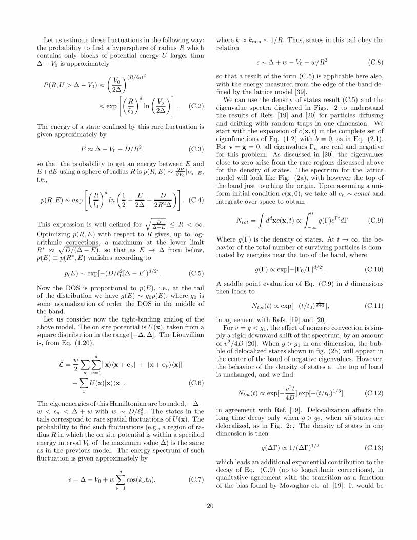
Let us estimate these fluctuations in the following way:the probability to find a hypersphere of radius R whichcontains only blocks of potential energy U larger than∆− V0 is approximately

P (R,U > ∆− V0) ≈(

V0

2∆

)(R/ℓ0)d

≈ exp

[

(

R

ℓ0

)d

ln

(

Vo

2∆

)

]

. (C.2)

The energy of a state confined by this rare fluctuation isgiven approximately by

E ≈ ∆− V0 −D/R2, (C.3)

so that the probability to get an energy between E andE+dE using a sphere of radius R is p(R,E) ∼ ∂P

∂V0|V0=E ,

i.e.,

p(R,E) ∼ exp

[

(

R

l0

)d

ln

(

1

2− E

2∆− D

2R2∆

)

]

. (C.4)

This expression is well defined for√

D∆−E ≤ R < ∞.

Optimizing p(R,E) with respect to R gives, up to log-arithmic corrections, a maximum at the lower limitR∗ ≈

√

D/(∆− E), so that as E → ∆ from below,p(E) ≡ p(R∗, E) vanishes according to

p(E) ∼ exp[−(D/ℓ20[∆− E])d/2]. (C.5)

Now the DOS is proportional to p(E), i.e., at the tailof the distribution we have g(E) ∼ g0p(E), where g0 issome normalization of order the DOS in the middle ofthe band.Let us consider now the tight-binding analog of the

above model. The on site potential is U(x), taken from asquare distribution in the range [−∆,∆]. The Liouvillianis, from Eq. (1.20),

L =w

2

∑

x

d∑

ν=1

[|x〉〈x + eν | + |x+ eν〉〈x|]

+∑

x

U(x)|x〉〈x| . (C.6)

The eigenenergies of this Hamiltonian are bounded, −∆−w < ǫn < ∆ + w with w ∼ D/ℓ20. The states in thetails correspond to rare spatial fluctuations of U(x). Theprobability to find such fluctuations (e.g., a region of ra-dius R in which the on site potential is within a specifiedenergy interval V0 of the maximum value ∆) is the sameas in the previous model. The energy spectrum of suchfluctuation is given approximately by

ǫ = ∆− V0 + w

d∑

ν=1

cos(kνℓ0), (C.7)

where k ≈ kmin ∼ 1/R. Thus, states in this tail obey therelation

ǫ ∼ ∆+ w − V0 − w/R2 (C.8)

so that a result of the form (C.5) is applicable here also,with the energy measured from the edge of the band de-fined by the lattice model [39].We can use the density of states result (C.5) and the

eigenvalue spectra displayed in Figs. 2 to understandthe results of Refs. [19] and [20] for particles diffusingand drifting with random traps in one dimension. Westart with the expansion of c(x, t) in the complete set ofeigenfunctions of Eq. (1.2) with b = 0, as in Eq. (2.1).For v = g = 0, all eigenvalues Γn are real and negativefor this problem. As discussed in [20], the eigenvaluesclose to zero arise from the rare regions discussed abovefor the density of states. The spectrum for the latticemodel will look like Fig. (2a), with however the top ofthe band just touching the origin. Upon assuming a uni-form initial condition c(x, 0), we take all cn ∼ const andintegrate over space to obtain

Ntot =

∫

ddxc(x, t) ∝∫ 0

−∞

g(Γ)eΓtdΓ (C.9)

Where g(Γ) is the density of states. At t → ∞, the be-havior of the total number of surviving particles is dom-inated by energies near the top of the band, where

g(Γ) ∝ exp[−|Γ0/Γ|d/2]. (C.10)

A saddle point evaluation of Eq. (C.9) in d dimensionsthen leads to

Ntot(t) ∝ exp[−(t/t0)d

d+2 ], (C.11)

in agreement with Refs. [19] and [20].For v = g < g1, the effect of nonzero convection is sim-

ply a rigid downward shift of the spectrum, by an amountof v2/4D [20]. When g > g1 in one dimension, the bub-ble of delocalized states shown in fig. (2b) will appear inthe center of the band of negative eigenvalues. However,the behavior of the density of states at the top of bandis unchanged, and we find

Ntot(t) ∝ exp[−v2t

4D] exp[−(t/t0)

1/3] (C.12)

in agreement with Ref. [19]. Delocalization affects thelong time decay only when g > g2, when all states aredelocalized, as in Fig. 2c. The density of states in onedimension is then

g(∆Γ) ∝ 1/(∆Γ)1/2 (C.13)

which leads an additional exponential contribution to thedecay of Eq. (C.9) (up to logarithmic corrections), inqualitative agreement with the transition as a functionof the bias found by Movaghar et. al. [19]. It would be

20

interesting to use the spectra displayed in Figs. 2 and3 to extract the short and intermediate time behavior ofNtot, as well as the effect of drift in higher dimensions.

Note that the delocalization transition which describesparticles diffusing and convecting in the presence of trapsoccurs at the top of the band. For population biologyproblems, one must consider positive growth eigenval-ues and the phenomena of interest typically occur forg1 < g < g2. The localization transition of interest to usin this paper occurs when the mobility edge crosses theorigin, as in Fig. 5.

[1] J. D. Murray, Mathematical Biology (Springer-Verlag,N.Y., 1993).

[2] A. J. Koch and H. Meinhardt, Rev. Mod. Phys. 66, 1481(1994). See also Sec. XI of M.C. Cross and P.E. Hohen-berg, Rev. Mod. Phys. 65 (1993).

[3] A recent exception is the numerical study of the effectof quenched randomness on Turing patterns in reaction-diffusion systems by I. Bose and I. Chaudhuri, cond-mat/9702230; see also M.W. Deem and J.M. Park, cond-mat/9707254.

[4] R. A. Fisher, Ann. Eugenics 7, 353 (1937).[5] A. Kolmogoroff, I. Petrovsky and N. Piscounoff, Moscow

Univ. Bull. Math. 1, 1 (1937).[6] See, e.g. J.D. Gunton, M. San Miguel and P.S. Sahni, in

Phase Transition and Critical Phenomena, vol. 8, editedby C. Domb and J. Liebowitz (Academic, New York,1983).

[7] To see why c(x, t) ≥ 0, suppose c(x, t) is initially non-negative but about to pass through zero at a point x0,i.e., c(x0, t) = 0+ and ∂c(x0,t)

∂t< 0. However, all terms

in Eq. (1.2) except the Laplacian then vanish at thispoint. If c(x0, t) is not identically zero in the vicin-ity of the point x0, then x0 is a local minimum and∂c(x0,t)

∂t= D∇2u(x0, t) > 0 which contradicts the as-

sumption that ∂c(x0,t)∂t

< 0.[8] C. H. Li and M. O. Robbins, Phys. Rev. B46, 14519

(1992).[9] D. T. Natterman, S. Stepanow, L.-H. Tang and H.

Leschom, J. Phys. (France) II 2, 1483 (1992).[10] O. Narayan and D. S. Fisher, Phys. Rev.B48, 7030

(1993).[11] G. Grinstein, Z.-W. Lai and D. A. Browne, Phys. Rev.

A40, 4820 (1989). See also, M. A. Munoz and T. Hwa,cond-mat/9702217.

[12] It should be noted that we study here growth of contin-uous populations, while the actual process is certainlydiscrete — the spreading of a gene, as well as the changeof the population, comes, of course, in quanta of oneor more individuals, and are not continuous variables.Throughout this paper, we neglect this effect and studyonly the continuum process. Discreteness can be modeledby inclusion of a multiplicative Langevin noise term, see,

e.g. V. Privman, Trends in Stat. Phys. 1 (1994); J. Cardy,cond-mat/9607163; J. Cardy and Uwe C. Tauber, cond-mat/9609151.

[13] J.-I. Wakita, K. Komatsu, A. Nakahara, T. Matsuyamaand M. Matsushita, J. Phys. Soc. Japan, 63, 1205 (1994).

[14] H. Berg, Random Walks in Biology (Princeton UniversityPress, Princeton, New Jersey 1993).

[15] J. Miller and J. Wang, Phys. Rev. Lett. 76, 1461 (1996);J.T. Chalker and J. Wang, cond-mat./9704198. See alsoD.S. Fisher, Phys. Rev. A 30, 960 (1984) and J.A.Aronovitz and D.R. Nelson, Phys. Rev. A 30, 1948(1984).

[16] D. R. Nelson and P. Le Doussal, Phys. Rev. B 42, 10113(1990); For a related treatment of convection of a passivescalar, see B. Shraiman and E.D. Siggia, Phys. Rev. E49,2912 (1994).

[17] D.R. Nelson and V.M. Vinokur, Phys. Rev. B 48, 13060(1993).

[18] D. Haarer and H. Mohrwald, Phys. Rev. Lett. 34, 1447(1975).

[19] B. Movaghar, G.W. Sauer and D. Wurtz, J. Stat. Phys.27, 473 (1982); B. Movaghar B. Pohlman and D. Wurtz,Phys. Rev. A 29, 1568 (1984).

[20] P. Grassberger and I Procaccia, J. Chem. Phys. 77, 6281(1982); Phys. Rev. A 26, 3686 (1982).

[21] L. W. Chen, L. Balents, M.P.A. Fisher and M. C.Marchetti, Phys. Rev. B54, 12798 (1996).

[22] K. B. Efetov, Phys. Rev. Lett. 79, 491 (1997),cond.-mat/9702091; J. Feinberg and A. Zee, cond.-mat/9703087; R. A. Janik, M. A. Nowak, G. Pappand I. Zahed, cond.-mat/9705098; J. Feinberg andA. Zee/9706218; I. V. Goldsheid and B. A. Khoruzhenko,cond-mat/9707230; and Ref. [30].

[23] B. I. Shklovskii and A.L. Efros, Electronic Properties of

Doped Semiconductors (Springer-Verlag, N.Y., 1984).[24] A similar transformation has been used for Fokker-Planck

equations by, e.g., P. G. de Gennes, J. Stat. Phys. 12, 463(1975); See also H. Risken, The Fokker-Planck Equation

(Springer, Berlin, 1984) Chapter 5. For the applicationto localized states, see P. Le Doussal (unpublished), andAppendix A of Ref. [21].

[25] N. Hatano and D. R. Nelson, Phys. Rev. Lett. 77 5701996; N. Hatano and D. R. Nelson, cond-mat/9705290(Phys. Rev. B, in press).

[26] D. Forster, D. R. Nelson and M. Stephen, Phys. Rev.A16, 732 (1977).

[27] See, e.g. G.B. Whitham, Linear and Nonlinear Waves

(Wiley, New York, 1974), Chapter 4.[28] See, e.g., F. R. Gantmacher, The Theory of Matrices,

Chelsea Publishing Company, N.Y. (1974).[29] K. G. Wilson and J. Kogut, Physics Reports, 12C, 77

(1974).[30] P.W. Brouwer, P.G. Silvestron and C.W.J. Beenakker,

cond-mat/9705186.[31] T. Hwa, D.R. Nelson and V. Vinokur, Phys. Rev. B48,

1167 (1993).[32] N. Shnerb and D.R. Nelson, to be published.[33] See, e.g., T. Halpin-Healy and Y. Zhang, Phys. Rep. 254,

215 (1995); D. S. Fisher, in Phase Transitions and Relax-

ation in Systems with Competing Energy Scales, Edited

21

by T. Riste and D. Sherrington (Kluwer, Boston 1993);and M. Kardar and Y.-C. Zhang, Phys. Rev. Lett. 58,2087 (1987).

[34] For an analysis of sample-to-sample fluctuations in thegrowth spectrum in one dimension at intermediate val-ues of v, see Ref. [30].

[35] See, e.g. R. Shankar, Principles of Quantum Mechanics,(Plenum, New York, 1980).

[36] L.-H. Tang, M. Kardar and D. Dhar, Phys. Rev. Lett.74, 920 (1995).

[37] S. P. Obukhov, Physica A 101, 145 (1980)[38] See, e.g., R. Friedberg and J.M. Luttinger, Phys. Rev. B

12 4460 (1975).[39] For a numerical evaluation of the density of states in the

one-dimensional lattice model, see T. Saso et al., Prog.Theor. Phys. (Supplement) 84, 269 (1985).

2

22