nonlinear analysis of beams using least-squares finite...

NONLINEAR ANALYSIS OF BEAMS USING LEAST-SQUARES FINITE

ELEMENT MODELS BASED ON THE EULER-BERNOULLI AND

TIMOSHENKO BEAM THEORIES

A Thesis

by

AMEETA AMAR RAUT

Submitted to the Office of Graduate Studies of

Texas A&M University

in partial fulfillment of the requirements for the degree of

MASTER OF SCIENCE

December 2009

Major Subject: Mechanical Engineering

NONLINEAR ANALYSIS OF BEAMS USING LEAST-SQUARES FINITE

ELEMENT MODELS BASED ON THE EULER-BERNOULLI AND

TIMOSHENKO BEAM THEORIES

A Thesis

by

AMEETA AMAR RAUT

Submitted to the Office of Graduate Studies of

Texas A&M University

in partial fulfillment of the requirements for the degree of

MASTER OF SCIENCE

Approved by:

Chair of Committee, J. N. Reddy

Committee Members, Ibrahim Karaman

Jose Roesset

Head of Department, Dennis O’Neal

December 2009

Major Subject: Mechanical Engineering

iii

ABSTRACT

Nonlinear Analysis of Beams Using Least-Squares Finite Element Models Based

on the Euler-Bernoulli and Timoshenko Beam Theories.

(December 2009)

Ameeta Amar Raut, B.E., Government College of Engineering, Pune, India

Chair of Advisory Committee: Dr. J. N. Reddy

The conventional finite element models (FEM) of problems in structural

mechanics are based on the principles of virtual work and the total potential

energy. In these models, the secondary variables, such as the bending moment

and shear force, are post-computed and do not yield good accuracy. In addition,

in the case of the Timoshenko beam theory, the element with lower-order equal

interpolation of the variables suffers from shear locking. In both Euler-Bernoulli

and Timoshenko beam theories, the elements based on weak form Galerkin

formulation also suffer from membrane locking when applied to geometrically

nonlinear problems. In order to alleviate these types of locking, often reduced

integration techniques are employed. However, this technique has other

disadvantages, such as hour-glass modes or spurious rigid body modes. Hence,

it is desirable to develop alternative finite element models that overcome the

locking problems. Least-squares finite element models are considered to be

better alternatives to the weak form Galerkin finite element models and,

therefore, are in this study for investigation. The basic idea behind the least-

iv

squares finite element model is to compute the residuals due to the

approximation of the variables of each equation being modeled, construct

integral statement of the sum of the squares of the residuals (called least-squares

functional), and minimize the integral with respect to the unknown parameters

(i.e., nodal values) of the approximations. The least-squares formulation helps to

retain the generalized displacements and forces (or stress resultants) as

independent variables, and also allows the use of equal order interpolation

functions for all variables.

In this thesis comparison is made between the solution accuracy of finite

element models of the Euler-Bernoulli and Timoshenko beam theories based on

two different least-square models with the conventional weak form Galerkin

finite element models. The developed models were applied to beam problems

with different boundary conditions. The solutions obtained by the least-squares

finite element models found to be very accurate for generalized displacements

and forces when compared with the exact solutions, and they are more accurate

in predicting the forces when compared to the conventional finite element

models.

v

// Shree Ganeshayanamaha //

To my beloved Mumma, Papa, Grandparents, Deepak

and

Dr. Reddy

vi

ACKNOWLEDGEMENTS

I wish to express my sincere gratitude to my advisor Dr. J. N. Reddy for

giving me an opportunity to work with him. His constant academic guidance,

encouragement and patience helped me learn and understand the coursework

which in turn greatly supported me in fulfillment of my research.

I would like to thank Dr. Jose Roesset and Dr. Ibrahim Karaman for

serving on my advisory committee. I really appreciate their constant support

and guidance.

I am thankful to Prof. Michael Golla of the Engineering Technology and

Industrial Distribution (ETID) department for giving me a valuable experience

of teaching and also financially supporting my entire education at Texas A&M

University. I deeply appreciate his help and kind consideration in my crucial

time.

I am also thankful to Ms. Missy Cornett for her kind help during my

studies.

My sincere thanks and appreciation to my mother and father to whom I

want to dedicate all my achievements for their unconditional love, support,

belief, encouragement and sacrifices. I am thankful to my grandparents and

family for their blessings and best wishes. I want to express my sincere

appreciation to Deepak for his unconditional patience and understanding

during my graduate studies.

Finally, I would like to thank all my friends and my colleagues at Texas

A&M University for their help and support during my stay in College Station.

vii

NOMENCLATURE

FEM Finite Element Method

EBT Euler-Bernoulli beam Theory

TBT Timoshenko Beam Theory

( )V x Internal Transverse Shear Force

xxN Internal Axial Force

xxM Internal Bending Moment

( )f x External Axial Force

( )q x Transverse Distributed Load

e

xxA Extensional Stiffness (EA)

e

xxB Extensional-Bending Stiffness

e

xxD Bending Stiffness (EI)

e

iQ Nodal Force

e

i∆ Nodal Displacement of the Element

eA Cross Sectional Area

eI Second Moment of Area of the Beam

jψ Lagrange Interpolation Functions

viii

jφ Hermite Interpolation Functions

R Residual Vector

T Tangent Matrix

ijσ Cartesian Component of Stress Tensor

ijε Cartesian Component of Strain Tensor

e

EW Work Done by External Forces

e

IW Work Done by Internal Forces

xxS Shear Stiffness (GAKs)

G Shear Modulus

E Young’s Modulus

Ks Shear Correction Factor

ix

TABLE OF CONTENTS

Page

ABSTRACT .............................................................................................................. iii

DEDICATION ......................................................................................................... v

ACKNOWLEDGEMENTS .................................................................................... vi

NOMENCLATURE ................................................................................................ vii

TABLE OF CONTENTS ......................................................................................... ix

LIST OF FIGURES .................................................................................................. xiii

LIST OF TABLES .................................................................................................... xvi

1. INTRODUCTION .......................................................................................... 1

1.1 Motivation .......................................................................................... 1

1.2 Objectives of the Present Study ....................................................... 2

1.3 Background and Literature Review ................................................ 2

2. ALTERNATIVE FINITE ELEMENT MODELS ......................................... 5

2.1 Introduction ....................................................................................... 5

2.2 Different Integral Formulations and Finite Element Models ..... 6

2.3 Summary............................................................................................ 8

3. THEORETICAL FORMULATION OF EBT AND TBT ............................ 9

3.1 Background ....................................................................................... 9

x

Page

3.2 Euler-Bernoulli Beam Theory ........................................................... 10

3.2.1 Assumptions ......................................................................... 10

3.2.2 Displacement fields .............................................................. 11

3.2.3 Nonlinear strain-displacement relations........................... 11

3.2.4 Derivation of governing equations ................................... 12

3.2.5 Vector approach .................................................................... 15

3.3 Timoshenko Beam Theory ................................................................ 16

3.3.1 Assumptions ......................................................................... 16

3.3.2 Displacement fields .............................................................. 17

3.3.3 Nonlinear strain-displacement relations........................... 17

3.3.4 Derivation of governing equations .................................... 18

3.4 Summary.............................................................................................. 20

4. FINITE ELEMENT MODEL OF THE EBT ................................................ 21

4.1 Weak Form Development ................................................................. 21

4.2 Finite Element Model ......................................................................... 22

4.3 Membrane Locking ............................................................................ 25

4.4 Summary.............................................................................................. 26

5. FINITE ELEMENT MODEL OF THE TBT ................................................ 27

5.1 Weak Form Development ................................................................ 27

5.2 Finite Element Model ........................................................................ 28

5.3 Shear and Membrane Locking ......................................................... 30

5.4 Summary............................................................................................. 31

6. LEAST-SQUARES THEORY & FORMULATION .................................... 32

6.1 Introduction ........................................................................................ 32

6.2 Basic Idea ............................................................................................ 32

6.3 Least-squares Finite Element MODEL 1 for Euler-Bernoulli

Beam Theory ...................................................................................... 35

xi

Page

6.3.1 Linear formulation ................................................................ 35

6.3.2 Nonlinear formulation .......................................................... 37

6.4 Least-squares Finite Element MODEL 1 for Timoshenko

Beam Theory ........................................................................................ 42



6.5 Least-squares Finite Element MODEL 2 for Euler-Bernoulli

Beam Theory ........................................................................................ 49



6.6 Least-squares Finite Element MODEL 2 for Timoshenko

Beam Theory ....................................................................................... 56

6.6.1 Linear formulation ............................................................... 56

6.6.2 Nonlinear formulation ......................................................... 58

7. SOLUTION APPROACH ............................................................................ 64

7.1 Solution Procedures .......................................................................... 64

7.1.1 Direct iteration procedure .................................................. 64

7.1.2 Newton-Raphson iteration procedure ............................. 64

8. DISCUSSION OF NUMERICAL RESULTS .............................................. 68

8.1. Example ............................................................................................. 68

8.2. Results ................................................................................................ 68

8.3. Plots .................................................................................................... 83

9. SUMMARY AND CONCLUSIONS .......................................................... 101

9.1. Future Work ..................................................................................... 102

REFERENCES ........................................................................................................ 103

APPENDIX A .......................................................................................................... 105

xii

Page

VITA ......................................................................................................................... 106

xiii

LIST OF FIGURES

Page

Figure 3.1 Deformation of a beam in Euler-Bernoulli theory .......................... 11

Figure 3.2 (a) Nodal displacements for EBT (b) Nodal forces for EBT ......... 13

Figure 3.3 A typical beam element with forces and moments under

uniformly distributed load ................................................................. 15

Figure 3.4 Deformation of a beam in Timoshenko theory ................................ 17

Figure 6.1 A typical beam element with forces and moments under

uniformly distributed load ................................................................. 33

Figure 7.1 A computer implementation flowchart ............................................ 67

Figure 8.1 Comparison of x vs. deflection in different models for

EBT, clamped-clamped, 4 elements .................................................. 83


TBT, clamped-clamped, 4 elements .................................................. 84


EBT, clamped-clamped, 8 elements .................................................. 85


TBT, clamped-clamped, 8 elements .................................................. 85


EBT, clamped-clamped 32 elements ................................................. 86


TBT, clamped-clamped 32 elements ................................................. 87


xiv

Page

EBT, hinged-hinged, 4 elements ....................................................... 88


TBT, hinged-hinged, 4 elements ........................................................ 89


EBT, hinged-hinged, 8 elements ........................................................ 90


TBT, hinged-hinged, 8 elements ...................................................... 90


EBT, hinged-hinged 32 elements ..................................................... 91


TBT, hinged-hinged 32 elements .................................................... 92


EBT, pinned-pinned, 4 elements ..................................................... 93


TBT, pinned-pinned, 4 elements .................................................... 93


EBT, pinned-pinned, 8 elements .................................................... 94


TBT, pinned-pinned, 8 elements .................................................... 95


EBT, pinned-pinned 32 elements .................................................... 96


TBT, pinned-pinned 32 elements ................................................... 96

xv

Page

Figure 8.19 Comparison of q vs. maximum deflection for EBT and TBT

for hinged-hinged boundary conditions ....................................... 97


for clamped-clamped boundary conditions ................................. 98


for pinned-pinned boundary conditions ...................................... 98

Figure 8.22 Comparison of x vs. Shear force for LSFEM MODEL2 and

conventional method ........................................................................ 99

Figure 8.23 Comparison of x vs. Bending Moments for LSFEM MODEL2

and conventional method ................................................................ 100

xvi

LIST OF TABLES

Page

Table 8.1 Comparison of displacements in EBT and TBT for

hinged-hinged beam .............................................................................. 68

Table 8.2 Comparison of displacements and forces in EBT for


Table 8.3 Comparison of displacements and forces in TBT for

hinged-hinged beam ............................................................................. 69


hinged-hinged beam ............................................................................. 70



Table 8.6 Comparison of displacements in EBT and TBT for

clamped-clamped beam ........................................................................ 72






clamped-clamped beam ....................................................................... 73


clamped-clamped beam ..................................................................... 74

Table 8.11Comparison of displacements in EBT and TBT for

pinned-pinned beam ............................................................................ 75


xvii

Page

pinned-pinned beam ........................................................................... 75







Table 8.16 A comparison of results for deflection of beams with

pinned-pinned boundary conditions under uniformly

distributed load for EBT ..................................................................... 78


pinned-pinned boundary conditions under uniformly

distributed load for TBT .................................................................... 79


hinged-hinged boundary conditions under uniformly

distributed load for EBT ...................................................................... 80


hinged-hinged boundary conditions under uniformly

distributed load for TBT ..................................................................... 81


clamped-clamped boundary conditions under uniformly

distributed load for EBT ..................................................................... 81


clamped-clamped boundary conditions under uniformly

distributed load for TBT ..................................................................... 82

1

1. INTRODUCTION

1.1 Motivation

The finite element method (FEM) is a powerful technique originally

developed for numerical solution of complex problems in structural mechanics.

The two broad categories into which finite element models can be divided are

those based on minimization principles (like in structural mechanics) [1,2] and

those based on weighted-residual methods such as the Galerkin method, Petrov-

Galerkin method, subdomain method, least-squares method and so on.

There are some numerical challenges that are encountered with

conventional finite element models based on the weak form Galerkin

formulation, which is the most common in practice. In these models, the

secondary variables such as the bending moment and shear force are post-

computed, typically at Gauss points and not at the nodes, and do not yield good

accuracy. In addition, in the case of the Timoshenko beam theory, the element

with lower-order equal interpolation of the generalized displacements suffers

from shear locking. In both Euler-Bernoulli and Timoshenko beam theories, the

elements based on the weak form Galerkin formulation also suffer from

membrane locking [3,4] when applied to geometrically nonlinear problems. Both

types of locking are a result of using inconsistent interpolation for the variables

involved in the formulation. In order to alleviate these types of locking, often

reduced integration techniques are employed. However, such ad-hoc techniques

have other disadvantages, such as hour-glass modes or spurious rigid body

modes.

This thesis follows the style and format of Finite Elements in Analysis and Design.

2

Thus, it is desirable to develop alternative finite element models that

overcome the locking problems and yield good accuracy for stress resultants.

Least-squares finite element models are considered to be alternatives to the

weak form Galerkin finite element model and thus considered in this study for

investigation. The least-squares formulation helps to retain the generalized

displacements and forces (or stress resultants) as independent variables, and

also allows the use of equal order interpolation functions for all variables.

1.2 Objectives of the Present Study

The purpose of this study is to investigate the effectiveness of the least-

squares based finite element models in solving the beam bending problems to

overcome shear and membrane locking and predict generalized forces

accurately. This study is conducted using the Euler-Bernoulli and Timoshenko

beam theories applied to straight beams. The solution accuracy of the least-

squares finite element models with conventional finite element models is also

assessed.

To achieve the defined objectives, different finite element models of the

two beam theories are developed and are applied to beam problems with

different boundary conditions. The solution obtained by the least-squares

formulation is compared to the solutions obtained from the conventional, weak

form Galerkin finite element models.

The following discussion provides the background for the present study.

1.3 Background and Literature Review

A beam is a structural element that has a very large ratio of its length to

its cross sectional dimension and is capable of carrying loads by stretching along

its length and bending about an axis transverse to its length. When transverse

3

loads are applied on a beam, internal forces are generated which resist the

deformation of the beam. If the applied load is large, the magnitude of the

internal forces increases. At the same time the deformation of the beam also

increases. Consequently, the linear relationship between loads and

displacements of the beam is no longer valid.

Depending on the kinematic assumptions, two different theories are often

used to model the structural behavior of beams:

1) Euler- Bernoulli beam theory (EBT)

2) Timoshenko beam theory(TBT)

In the Euler Bernoulli beam theory, one neglects the effect of the transverse

shear strain whereas in the Timoshenko beam theory it is taken into account.

Both shear and membrane locking in beams are primarily due to the use

of inconsistent interpolation of the variables. When equal and lower order

interpolation of the displacement and rotation are used in the Timoshenko beam

finite element, the element exhibits locking as it is unable to cope with the

constraint that the slope should be compatible with the derivative of the

deflection in the thin beam limit. The problem of shear locking is often overcome

by numerically mimicking different variation (i.e., constant and linear) of the

rotation function in shear energy and bending energy through numerical

integration [2]. There are several other approaches that have been adopted to

eliminate locking [1, 2, 5-10]. The concept of locking was first discussed by

Kikuchi and Aizawa [5], and Zienkiewicz and Owen [11] advocated that the

reduced integration technique is a means of obtaining accurate solutions.

However, such ad-hoc approaches have other disadvantages, such as

appearance of hour-glass modes or spurious rigid body modes. Hence, it is

4

desirable to develop alternative finite element models that overcome the locking

problems.

In the past few years finite element methods based on least-squares

variational principles have drawn considerable attention. It is a general

methodology that produces a wide range of algorithms [9]. Given a set of

differential equations, the least-squares method allows one to define a convex,

unconstrained minimization principle so that the finite element model can be

developed in Ritz or weak form Galerkin setting [2]. This model has proved to

result in a positive-definite system of equations and significant savings in the

computational cost [12].

The least-square approach has been implemented in the finite element

context to solve the problems of plate bending, shear-deformable shells,

incompressible and compressible fluid flows [1, 13-15] etc. However, there has

been no systematic study involving the development of least-squares finite

element models of beam theories and their assessment in comparison to the

conventional beam finite elements. The present study also accounts for

geometric nonlinearity in the von karaman sense.

5

2. ALTERNATIVE FINITE ELEMENT MODELS

2.1 Introduction

A mathematical model is a set of equations, algebraic as well as

differential, which is used to describe the response of a physical system in terms

of certain variables. The mathematical models of most mechanical systems are

derived using the principles of physics, such as the conservation of mass,

conservation of linear momentum, and conservation of energy. The derivation

of the governing equations is not as challenging as solving them and computing

accurate solution. Numerical methods help to convert these governing

differential equations to a set of algebraic equations that can be solved using

computers. While solving such equations proper care must be taken to preserve

all features of the mathematical model (which reflects the physics of the

problem) in the formulation and development of the associated computational

model.

There are several methods to obtain numerical solutions of ordinary and

partial differential equations. These include the finite difference method, traditional

variational methods (e.g., Ritz and Galerkin methods), the finite element method, etc. In

the finite difference method, the derivatives in the governing differential

equations are replaced by discrete values. In a variational approach, the

variable(s) of a differential equation are approximated as a linear combination of

unknown parameters and known functions, 0

1

( ) ( ) ( ) ( )

n

j j

j

u x U x c x xφ φ=

≈ = +∑ , and the

parameters i

c are then determined by satisfying the differential equations in a

weighted-residual sense (see Reddy [3]). In the finite element method, the

domain of the problem is divided into a collection of subdomains (called finite

6

elements), and over each subdomain a variational method is used to set up the

discrete problem. The element equations are then put together to obtain a

system of algebraic equations for the assemblage of elements. Different types of

finite element models are obtained by using different weighted-integral

statement. These are discussed in the following section.

2.2 Different Integral Formulations and Finite Element Models

Based on the method used to derive the algebraic equations of a

mathematical model, different finite element models of the mathematical model

can be developed. These alternative methods are discussed next.

1) The Ritz Method: Here the coefficients of the approximation are

determined by minimizing a functional (i.e., first variation of I is equal to zero)

equivalent to the governing differential equation 0Au f− = ,

1

( ) ( , ) ( ), 0 ( , ) ( )2

I u B u u l u I B u u l uδ δ δ= − = ⇒ = (1)

Then the approximations

( ) ( ) ( ) ( )0

1 1

( ) ,N N

N j j j j

j j

u x U x c x x u c xφ φ δ δ φ= =

≈ = + ≈∑ ∑ (2)

are substituted for u and uδ into Eq. (1) to obtain the Ritz finite element model

( ) ( ) ( )( )

( ) ( )( ) ( )( ) ( ) ( )( )

( ) ( )( )( )( ) ( ) ( )( )

0

1

0

1

1

0

, ,

1, 2,3,....

, ,

,

N

j j i

j

N

j i j i i

j

N

ij j i

j

ij j i

i i i

B c x x l x

B x x c l x B x x

or K c F i N

K B x x

F l x B x x

φ φ φ

φ φ φ φ φ

φ φ

φ φ φ

=

=

=

+ =

= −

= =

=

= −

∑

∑

∑

7

2) Weighted Residual Method: In the weighted residual method, the

approximate solution is substituted into the differential equation 0Au f− = and

the resulting residual 0R AU f= − ≠ is minimized with respect to a weight

function. Depending on the choice of the weight function various models can be

derived. Various subclasses of the weighted residual method are summarized

below. In the general weighted-residual method, we require

( ) ( )x x, 0 ( 1,2..... )i jR c dxdy where i NψΩ

= =∫

where

( ) ( ) ( )0

1

0N

N j j

j

R A U f A c x x fφ φ=

≡ − = + − ≠

∑

(a) The Petrov-Galerkin Method The above weighted residual method is called

Petrov-Galerkin method when i iψ φ≠

( ) ( )0

j=1

N

i j j iA dx c f A dxψ φ ψ φΩ Ω

= − ∑ ∫ ∫

(b) The Galerkin Method: If i iψ φ= then the weighted residual method is called

Galerkin method.

( )

( )0

ij i j

i i

A A dx

F f A dx

φ φ

φ φ

Ω

Ω

=

= −

∫

∫

The approximation functions used here are of much higher order than the one

used in the Ritz method.

(c) The Collocation Method

Here the approximation functions are selected such that the residual will be

zero simultaneously. Thus we have ( ), 0 ( 1,2.... )i

jR x c i N= = .

8

(d) The Least-Squares Method

The basic concept behind the least squares method is that it minimizes the

square of the residual. The parameter j

c is determined by minimizing the

integral of the square of the residual.

( )2 x, 0j

i

R c dxc Ω

∂=

∂ ∫

where

2 2 2

1 2 1 2( ) ( ), ,h h

R R R R A u f R B u g= + = − = − and

( ) ( ) in and B in A u f u g= Ω = Γ are the functions.

In the present study, the least squares method is used to formulate the finite

element models of the Euler-Bernoulli beam theory (EBT ) and the Timoshenko

beam theory (TBT).

2.3 Summary

Thus FEM is a numerical method that can be a used to obtain a

numerical solution where an analytical solution cannot be developed. FEM was

originally developed for analysis of aircraft structures. However due to its

general nature it has been applicable in a wide range of problems in structural

mechanics, fluid mechanics, electrical engineering etc. This section discusses

different types of formulations in finite element analysis. This thesis will discuss

more about the theory, formulations and finite element model for least-squares

based finite element formulation in details in the subsequent sections. This

study will be conducted specifically for beams as they are widely used in many

structural applications.

9

3. THEORETICAL FORMULATION OF EBT AND TBT

3.1 Background

A beam is a structural element that has a very large ratio of its length to

its cross section dimension. It can be subjected to a transverse load which

includes the normal and the shear stress and the displacements are

perpendicular to the normal axis. Beams can be straight or curved. A straight

beam is usually modeled by a line segment with vertical displacement and

rotations at each end.

When the load is applied on a beam, internal forces are generated which

resist the deformation of the beam. If the applied load is large, the magnitude of

the internal forces increases. At the same time the deformation of the beam also

increases. Thus the linear relationship between load v/s deflection of the beam is

no more valid.

The following assumptions are made in the development of linear motion of

solid bodies:

1) The displacements are small.

2) The strains developed are very large.

3) The material is linearly elastic.

Due to the small strains the changes in the geometry are ignored. The

equilibrium equations are developed for the undeformed configuration. But if

the load increases the linear relationships do not hold true. Hence for a general

nonlinear formulation of straight or curved beams, the measures of stress and

strain consistent with the deformations must be accounted in the formulation.

The following assumptions are made in the study of nonlinear analysis of beams

here:

10

1) The beam is long and thin

2) The transverse displacements are large.

3) The strains developed are very small.

4) The rotations developed are small.

The inplane forces are proportional to the square of the rotation of the transverse

normal to the beam axis and are responsible for the nonlinearity.

Depending on the assumptions for transverse shear strain there are two

different theories to model the beams:

3) Euler- Bernoulli beam theory (EBT)

4) Timoshenko beam theory(TBT)

The Euler Bernoulli beam theory neglects the effect of the transverse shear strain

whereas the Timoshenko beam theory takes into account the effect of transverse

shear strain in the formulation.

3.2 Euler-Bernoulli Beam Theory

EBT is the simplest beam theory and is based on displacement field. The

following sections will discuss about EBT in detail.

3.2.1 Assumptions

The basic assumptions made in developing the governing equations of EB

hypothesis are the plane cross sections perpendicular to the beam axis before

deformation remain (a) plane (b) rigid (c) rotate such that they remain

perpendicular to the beam axis after deformation.

These assumptions neglect the Poisson’s effect and the transverse strain.

These two assumptions are taken into account in Timoshenko beam theory.

11

x

z, w0

x,u0z

Undeformed

(u ,w )0 0

(u,w)

u0

-dw0

dx

-dw0

dx

EBT

Figure 3.1. Deformation of a beam in Euler-Bernoulli theory

3.2.2 Displacement fields

The displacement field for beams having moderately large rotations but

small strains derived from Figure 3.1 is:

01 0 ( )

dwu u x z

dx= − , 2 0u = and 3 0 ( )u w x= (3.1)

where, 1 2 3( , , )u u u are the displacement along (x, y, z) axis and

0u is the axial displacement of a point on the neutral axis and

0w is the transverse displacement of the point on the neutral axis

3.2.3 Nonlinear strain-displacement relations

The following nonlinear strain-displacement relation is used to calculate

the strains

1 1

2 2

ji m mij

j i i j

uu u u

x x x xε

∂∂ ∂ ∂= + + ∂ ∂ ∂ ∂

(3.2)

Substituting the values of 1u , 2u and 3u in the above equations and eliminating

the large strain terms but retaining the rotation terms of the transverse normal

we get,

12

22

0 0 011 2

1

2xx

du d w dwz

dx dx dxε ε

= = − +

2 2

0 0 0

2

1

2

du dw d wz

dx dx dx

= + −

0 1

xx xxzε ε= + (3.3)

where,

2 20 10 0 0

2

1,

2xx xx

du dw d w

dx dx dxε ε

= + = −

These strains are known as von Karman strains.

3.2.4 Derivation of governing equations

According to the principle of virtual displacement, for a body in

equilibrium, the virtual work done by the internal and external forces to move

through their virtual displacements is zero. Thus based on this principle the

following can be concluded.

0e e e

I EW W Wδ δ δ≡ + = (3.4)

where

e

IWδ is the virtual strain stored in the element due to

ijσ (Cartesian component

of stress tensor) due to the virtual displacement ij

δε (Cartesian component of

strain tensor) and

e

EWδ is the work done by external forces

Thus for a beam element we have,

e

e

I ij ijV

W dVδ δε σ= ∫

6

0 0

1

b

e

a

x

e e e

E i iV

ix

W q w dx f u dx Qδ δ δ δ=

= + + ∆∑∫ ∫ (3.5)

13

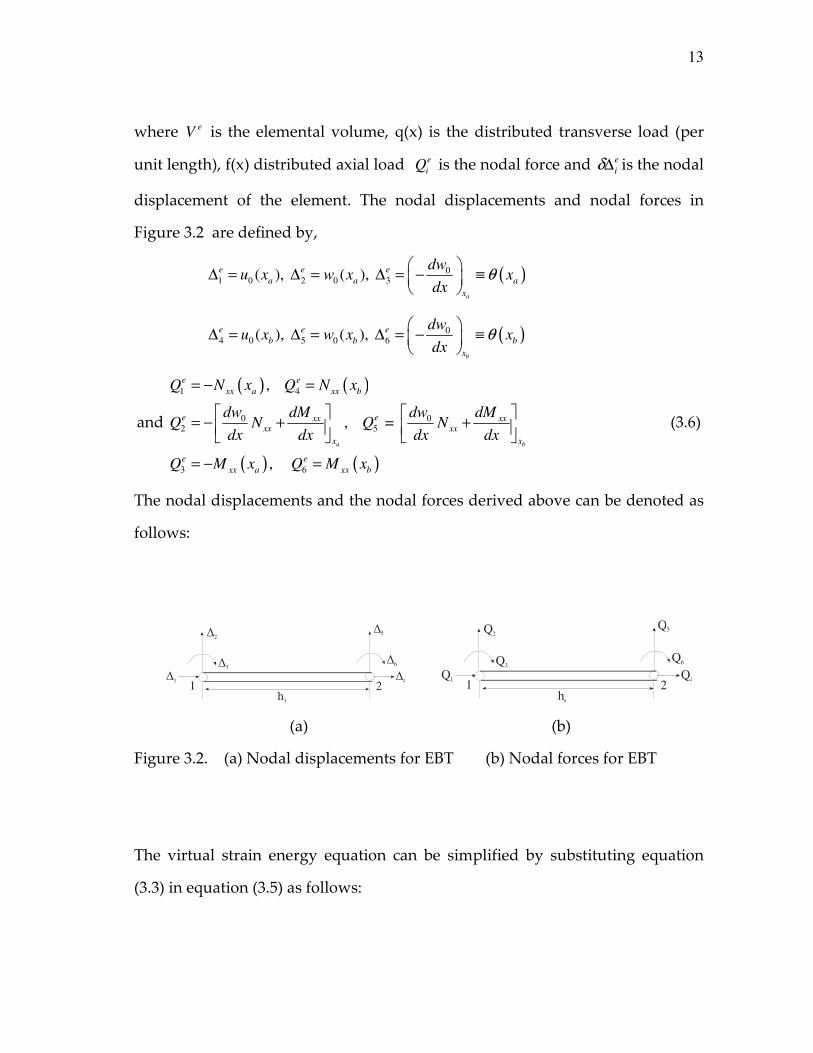
where eV is the elemental volume, q(x) is the distributed transverse load (per

unit length), f(x) distributed axial load e

iQ is the nodal force and e

iδ∆ is the nodal

displacement of the element. The nodal displacements and nodal forces in

Figure 3.2 are defined by,

( )01 0 2 0 3( ), ( ),

a

e e e

a a a

x

dwu x w x x

dxθ

∆ = ∆ = ∆ = − ≡

( )04 0 5 0 6( ), ( ),

b

e e e

b b b

x

dwu x w x x

dxθ

∆ = ∆ = ∆ = − ≡

and

( ) ( )

( ) ( )

1 4

0 02 5

3 6

,

, =

,

a b

e e

xx a xx b

e exx xxxx xx

x x

e e

xx a xx b

Q N x Q N x

dw dM dw dMQ N Q N

dx dx dx dx

Q M x Q M x

= − =

= − + +

= − =

(3.6)

The nodal displacements and the nodal forces derived above can be denoted as

follows:

1 2

∆1

∆2

∆3

∆4

∆5

∆6

h1 1 2

Q1

Q2

Q3

Q4

Q5

Q6

he

(a) (b)

Figure 3.2. (a) Nodal displacements for EBT (b) Nodal forces for EBT

The virtual strain energy equation can be simplified by substituting equation

(3.3) in equation (3.5) as follows:

14

b

ea

xe

I xx xxx A

W dAdxδ δε σ= ∫ ∫

( )0 1b

ea

x

xx xx xxx A

z dAdxδε δε σ= +∫ ∫

2

0 0 0 0

2

b

ea

x

xxx A

d u dw d w d wz dAdx

dx dx dx dx

δ δ δσ

= + +

∫ ∫

2

0 0 0 0

2

b

ea

x

xx xxx A

d u dw d w d wN M dx

dx dx dx dx

δ δ δ = + +

∫ ∫ (3.7)

here xx

N is the axial force which can be expressed as exx xx

AN dAσ= ∫ and

xxM is the moment which can be expressed as

exx xxA

M zdAσ= ∫

Thus virtual work statement can be written as

( ) ( )

( ) ( )

2

0 0 0 002

6

0

1

0

b

e

a

b

a

x

xx xxV

x

x

e e

i i

ix

d u dw d w d wN M dx q x w x dx

dx dx dx dx

f x u x dx Q

δ δ δδ

δ δ=

= + − − −

− ∆

∫ ∫

∑∫

(3.8)

By separating the two terms involving 0 0 and u wδ δ we get the following two

equations

( ) ( )

( ) ( )

00 1 1 4 2

2

0 0 00 2 2 3 3 5 1 6 22

0

0

b

a

b

a

x

e e e e

xx

x

x

e e e e e e e e

xx xx

x

d uN f x u x dx Q Q dx

dx

d w dw d wN M q x w x dx Q Q Q Q

dx dx dx

δδ δ δ

δ δδ δ δ δ δ

= − − ∆ − ∆

= − − − ∆ − ∆ − ∆ − ∆

∫

∫

(3.9)

Collecting the terms of 0uδ and 0wδ and simplifying the terms we get,

( )

( )

0

2

00 2

: -

: -

xx

xxxx

dNu f x

dx

dw d Mdw N q x

dx dx dx

δ

δ

=

− =

(3.10)

15

Thus the boundary conditions are:

( ) ( )

( ) ( )

1 4

0 02 5

3 6

0, 0

0, 0

+ =0 , + =0

a b

e e

xx a xx b

e exx xxxx xx

x x

e e

xx a xx b

Q N x Q N x

dw dM dw dMQ N Q N

dx dx dx dx

Q M x Q M x

+ = − =

+ + = − + =

(3.11)

3.2.5 Vector approach

In this method a beam element of length x∆ is analyzed by adding the

forces and the moments acting on the beam.

f(x)

q(x)

z

x

VV+∆V

N Nxx xx+∆

M Mxx xx+∆∆x

q(x)

dwdx

Mxx

Nxx

x

z

Figure 3.3. A typical beam element with forces and moments under uniformly

distributed load

Consider the above beam element with forces and moments under uniformly

distributed load is shown in Figure 3.3 where ( )V x is the internal vertical

shear force,

16

xxN is the internal axial force,

xxM is the internal bending moment,

( )f x is the external axial force,

( )q x is the distributed load.

Using D Alembert’s principle and equating the forces in the X, Y and Z direction

we get

( ) ( )

( ) ( )

( ) ( ) ( )0

0 : 0

0 : 0

0 : 0

x xx xx xx

y

z xx xx xx xx

F N N N f x x

F V V V q x x

dwF M M M V x N x q x x c x

dx

= − + + ∆ + ∆ =

= − + + ∆ + ∆ =

= − + + ∆ − ∆ + ∆ + ∆ ∆ =

∑∑

∑

Thus taking the limit as 0x∆ → we can conclude

( )

( )

0

0

0

0

xx

xxxx

dNf x

dx

dVq x

dx

dM dwV N

dx dx

+ =

+ =

− + =

(3.12)

3.3 Timoshenko Beam Theory

3.3.1 Assumptions

As discussed earlier, basic assumptions made in developing the

governing equations of EB hypothesis are the plane cross sections perpendicular

to the beam axis before deformation remains (a) plane (b) rigid (c) rotation is

independent of the slope of the beam. In TBT the first two assumptions are the

same and the third assumption is relaxed by assuming that the rotation of the

beam is independent of the slope.

17

3.3.2 Displacement fields

The displacement field for beams having moderately large rotations but

small strains as shown in Figure 3.4 is given by

( )1 0 ( ) xu u x z xφ= + , 2 0u = and 3 0 ( )u w x= (3.13)

where, 1 2 3( , , )u u u are the displacement along (x, y, z) axis, 0u is the axial

displacement of a point on the neutral axis, and 0w is the transverse

displacement of the point on the neutral axis.

x

z, w0

x,u0z

Undeformed

(u ,w )0 0

(u,w)

u0

-dw0

dxTBT

Φ

Figure 3.4. Deformation of a beam in Timoshenko theory

3.3.3 Nonlinear strain-displacement relations

The following nonlinear strain-displacement relation is used to calculate

the strains as follows

18

1 1

2 2

ji m mij

j i i j

uu u u

x x x xε

∂∂ ∂ ∂= + + ∂ ∂ ∂ ∂

(3.14)

Substituting the values of 1u , 2u and 3u in the above equations and eliminating

the large strain terms but retaining the rotation terms of the transverse normal

we get,

2

0 011

1

2

xxx

du d dwz

dx dx dx

φε ε

= = − +

2

0 01

2

xdu dw d

zdx dx dx

φ = + +

0 1

xx xxzε ε= + (3.15)

03 01xz x xz

u dwu

x x dxγ φ γ

∂∂= − = + ≡

∂ ∂ (3.16)

where 0 1 00 0 0 0, , xxx xx xz x

d u dw d w d d w

dx dx dx dx dx

δ δ δφ δδε δε δγ δφ

= + = = +

3.3.4 Derivation of governing equations

As discussed in EBT, the principle of virtual displacement states that for a

body in equilibrium, the virtual work done by the internal and external forces to

move through their virtual displacements is zero. Thus based on this principle

the following can be concluded.

0e e e

I EW W Wδ δ δ≡ + = (3.17)

where e

IWδ the virtual strain is stored in the element due to

ijσ (Cartesian

component of stress tensor) due to the virtual displacement ij

δε (Cartesian

component of strain tensor) and e

EWδ is the work done by external forces.

Thus for a beam element we have,

e

e

I ij ijV

W dVδ δε σ= ∫

19

6

0 0

1

b

e

a

x

e e e

E i iV

ix

W q w dx f u dx Qδ δ δ δ=

= + + ∆∑∫ ∫ (3.18)

where eV is the elemental volume, q(x) is the distributed transverse load (per

unit length), f(x) distributed axial load e

iQ is the nodal force and e

iδ∆ is the nodal

displacement of the element.

The virtual strain energy equation can be simplified as follows:

( )b

ea

xe

I xx xx xz xzx A

W dAdxδ δε σ δγ σ= +∫ ∫

( )0 1 0b

ea

x

xx xx xx xz xzx A

z dAdxδε δε σ δγ σ= + +∫ ∫

0 1 0b

ea

x

xx xx xx xx xz xx A

N M Q dxδε δε δγ = + + ∫ ∫ (3.19)

where xx

N is the axial force which can be expressed as exx xx

AN dAσ= ∫ and

xxM is the moment which can be expressed as exx xx

AM zdAσ= ∫

xQ is the element force x s xzA

Q K dAσ= ∫

sK is the shear correction coefficient which takes into account the difference

between the shear energy calculated by equilibrium and by Timoshenko beam

theory. Solving in the same way as EBT and collecting the terms of 0uδ and 0wδ

and simplifying the terms we get,

( )

( )

0

2

00 2

:

: 0

:

xx

xxxx

xxxx

dNu f x

dx

dMQ

dx

dw d Mdw N q x

dx dx dx

δ

δφ

δ

− =

− + =

− − =

(3.20)

20

3.4 Summary

This section discusses the introduction to beams and the different

assumptions made to derive the beam equation. A more detailed discussion

about the two most important theories Euler-Bernoulli and Timoshenko beam

theory regarding the derivation of the governing differential equations has been

made in this section. The discussion of weak form development and finite

element model for EBT and TBT has been done in the next section.

21

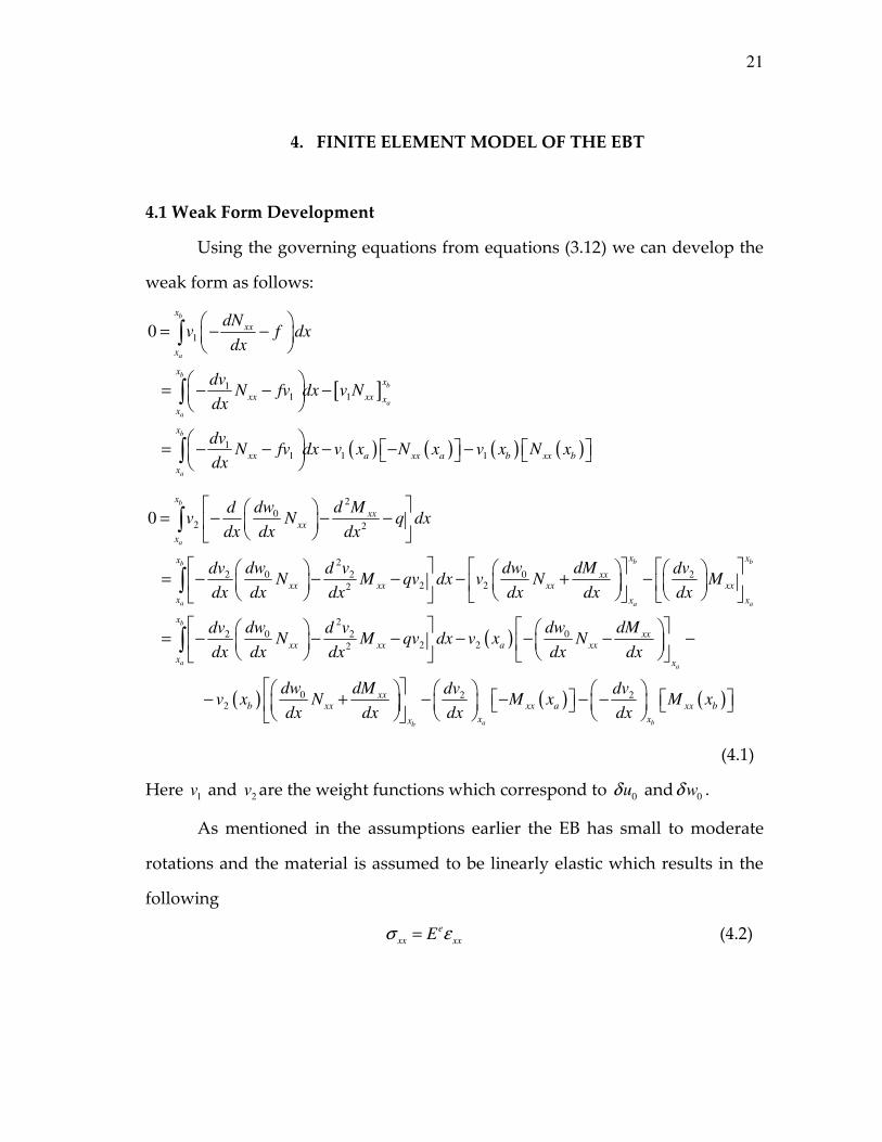
4. FINITE ELEMENT MODEL OF THE EBT

4.1 Weak Form Development

Using the governing equations from equations (3.12) we can develop the

weak form as follows:

[ ]

( ) ( ) ( ) ( )

1

11 1

11 1 1

0

b

a

b

b

a

a

b

a

x

xx

x

xx

xx xx x

x

x

xx a xx a b xx b

x

dNv f dx

dx

dvN fv dx v N

dx

dvN fv dx v x N x v x N x

dx

= − −

= − − −

= − − − − −

∫

∫

∫

2

02 2

2

0 02 2 22 22

2

02 222

0

b

a

b bb

a aa

x

xxxx

x

x xx

xxxx xx xx xx

x xx

xx xx

dw d Mdv N q dx

dx dx dx

dw dw dMdv d v dvN M qv dx v N M

dx dx dx dx dx dx

dwdv d vN M qv

dx dx dx

= − − −

= − − − − + −

= − − −

∫

∫

( )

( ) ( ) ( )

02

0 2 22

b

aa

a bb

x

xxa xx

x x

xxb xx xx a xx b

x xx

dw dMdx v x N

dx dx

dw dM dv dvv x N M x M x

dx dx dx dx

− − − −

− + − − − −

∫

(4.1)

Here 1v and 2v are the weight functions which correspond to 0uδ and 0wδ .

As mentioned in the assumptions earlier the EB has small to moderate

rotations and the material is assumed to be linearly elastic which results in the

following

e

xx xxEσ ε= (4.2)

22

The above relationship which defines the relationship between the total stress

and the total strain is called as the Hooke’s law.

Thus we get

2 2

0 0 0

2

2 2

0 0 0

2

1

2

1

2

e e

e

e

xx xx xxA A

e

A

e e

xx xx

N dA E dA

du dw d wE z dA

dx dx dx

du dw d wA B

dx dx dx

σ ε= =

= + −

= + −

∫ ∫

∫ (4.3)

2 2

0 0 0

2

2 2

0 0 0

2

1

2

1

2

e e

e

e

xx xx xxA A

e

A

e e

xx xx

M zdA E zdA

du dw d wE z zdA

dx dx dx

du dw d wB D

dx dx dx

σ ε= =

= + −

= + −

∫ ∫

∫ (4. 4)

where, e

xxA is the extensional stiffness

e

xxB is the extensional-bending stiffness and

e

xxD is the bending stiffness.

For isotropic material we have,

e e e

xxA E A= , 0e

xxB = and e e e

xxD E I= where eA is the cross section area and eI is

the second moment of inertia of the beam element.

4.2 Finite Element Model

The interpolation functions for the axial and transverse deflection will be

( ) ( )2

0

1

j j

j

u x u xψ=

=∑ And ( ) ( )4

0

1

j j

j

w x xφ=

= ∆∑ (4.5)

( ) ( ) ( ) ( )1 0 2 3 0 4, , , a a b bw x x w x xθ θ∆ ≡ ∆ ≡ ∆ ≡ ∆ ≡ (4.6)

23

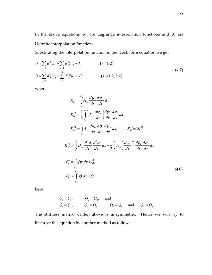
In the above equations jψ are Lagrange interpolation functions and jφ are

Hermite interpolation functions.

Substituting the interpolation function in the weak form equation we get

( )

( )

2 411 12 1

1 1

2 421 22 2

1 1

0 1,2

0 1, 2,3,4

ij j iJ J i

j J

Ij j IJ J I

j J

K u K u F i

K u K u F I

= =

= =

= + − =

= + − =

∑ ∑

∑ ∑ (4.7)

where

11

12 0

21 21 120

1

2

, =2

b

a

b

a

b

a

x

jiij xx

x

x

i JiJ xx

x

x

jIIj xx Ij iJ

x

ddK A dx

dx dx

dw d dK A dx

dx dx dx

ddw dK A dx K K

dx dx dx

ψψ

ψ φ

ψφ

=

=

=

∫

∫

∫

22222 0

2 2

1

2

b b

a a

x x

J JI IIJ xx xx

x x

d dw dd dK D dx A dx

dx dx dx dx dx

φ φφ φ = +

∫ ∫

1

2

ˆb

a

b

a

x

i i i

x

x

i I I

x

F f dx Q

F q dx Q

ψ

φ

= +

= +

∫

∫

(4.8)

here

1 1 2 2

1 3 2 4 3 5 4 6

ˆ ˆ, , and

, , and

Q Q Q Q

Q Q Q Q Q Q Q Q

= =

= = = =

The stiffness matrix written above is unsymmetric. Hence we will try to

linearize the equation by another method as follows,

24

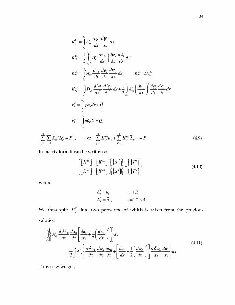
11

12 0

21 21 120

22222 0

2 2

1

1

2

, =2

1

2

b

a

b

a

b

a

b b

a a

a

x

je iij xx

x

x

e i JiJ xx

x

x

je IIj xx Ij iJ

x

x x

eJ JI IIJ xx xx

x x

x

i

x

ddK A dx

dx dx

dw d dK A dx

dx dx dx

ddw dK A dx K K

dx dx dx

d dw dd dK D dx A dx

dx dx dx dx dx

F f

ψψ

ψ φ

ψφ

φ φφ φ

=

=

=

= +

=

∫

∫

∫

∫ ∫

2

ˆb

b

a

i i

x

i I I

x

dx Q

F q dx Q

ψ

φ

+

= +

∫

∫

2 2 41 2

1 1 1 1

, or ip p i ip p iP P i

p p P

K F K u K Fαγ γ α α α α

γ = = = =

∆ = + ∆ + =∑∑ ∑ ∑ (4.9)

In matrix form it can be written as

1 111 12

21 22 2 2

FK K

K K F

∆ = ∆

(4.10)

where

1

2

, i=1,2

, i=1,2,3,4

i i

i i

u∆ =

∆ = ∆

We thus split 12

iJK into two parts one of which is taken from the previous

solution

2

0 0 0 0

2

0 0 0 0 0 0 0

1

2

1 1

2 2

b

a

b

a

x

e

xx

x

x

e

xx

x

d w dw du dwA dx

dx dx dx dx

d w dw du du dw d w dwA dx

dx dx dx dx dx dx dx

δ

δ δ

+

= + +

∫

∫

(4.11)

Thus now we get,

25

111 12

21 22 2

FK K u

K K F

= ∆

(4.12)

where

11 11

12 12 0

21 21 120

1

2

1, =

2

b

a

b

a

b

a

x

je iij ij xx

x

x

e i JiJ iJ xx

x

x

je IIj xx Ij iJ

x

ddK K A dx

dx dx

dw d dK K A dx

dx dx dx

ddw dK A dx K K

dx dx dx

ψψ

ψ φ

ψφ

= =

= =

=

∫

∫

∫

22222 0 0

2 2

1

2

1

2

ˆ

b b

a a

b

a

b

a

x x

eJ JI IIJ xx xx

x x

x

i i i

x

x

i I I

x

d dw du dd dK D dx A dx

dx dx dx dx dx dx

F f dx Q

F q dx Q

φ φφ φ

ψ

φ

= + +

= +

= +

∫ ∫

∫

∫

(4.13)

4.3 Membrane Locking

Linearity is one of the assumptions of the EBT. This means that the beam

is subjected to bending forces only and there are no axial forces. Thus ideally the

beam should not stretch. Thus the axial strain should be zero.

2 2

0 0 0 010 OR

2

du dw du dw

dx dx dx dx

+ =

In bending dominated deformations, the beam undergoes axial

displacement along with transverse deflection even when there are no axial

forces. In order to develop this transverse deflection the axial strain is developed

in the beam. Thus as the load increases the axial stiffness increases. This results

in computational difficulties and incorrect solutions. The inaccuracy in the

26

solution is because of the ambiguity between the degree of polynomial variation

and the interpolation functions of 0u and 0w . This phenomenon is called

membrane locking. A normal way to solve such problems is to take the

minimum interpolation of 0u and 0w .

4.4 Summary

This section discussed about the conventional weighted residual method

for Euler-Bernoulli (EB) beam theory. This part of the research focuses mainly on

the weak form development and finite element model. The element coefficients

obtained in this finite element model will be assembled to form a global stiffness

matrix and the solutions will be obtained by FORTRAN program. A detailed

discussion about the solution procedure has been made in this section. A similar

discussion about the Timoshenko beam theory (TBT) will be made in the

following section.

27

5. FINITE ELEMENT MODEL OF THE TBT

5.1 Weak Form Development

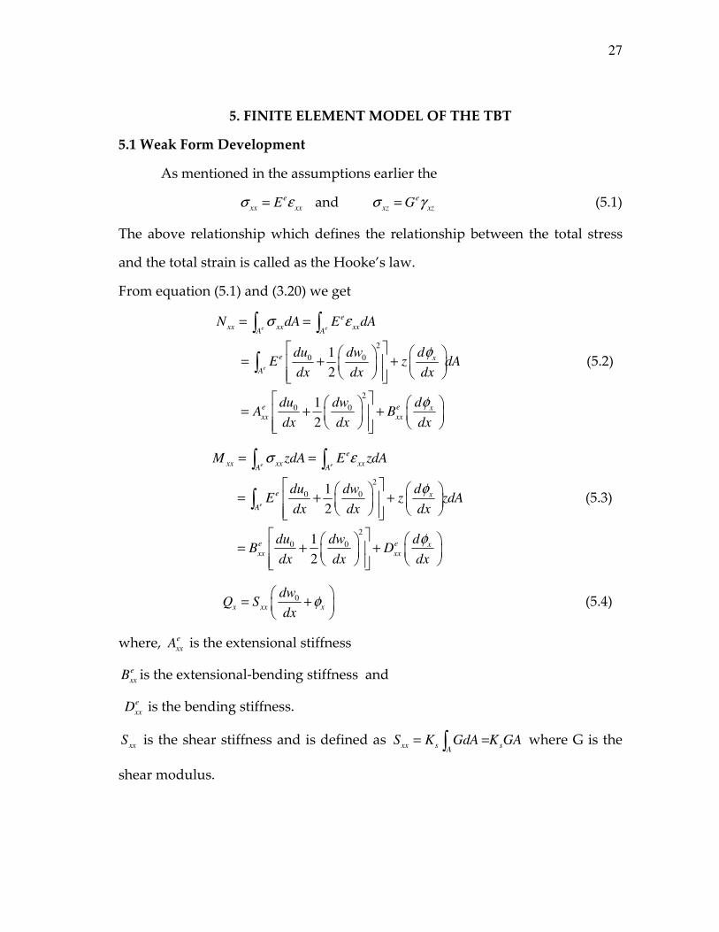
As mentioned in the assumptions earlier the

e

xx xxEσ ε= and e

xz xzGσ γ= (5.1)

The above relationship which defines the relationship between the total stress

and the total strain is called as the Hooke’s law.

From equation (5.1) and (3.20) we get

2

0 0

2

0 0

1

2

1

2

e e

e

e

xx xx xxA A

e x

A

e e xxx xx

N dA E dA

du dw dE z dA

dx dx dx

du dw dA B

dx dx dx

σ ε

φ

φ

= =

= + +

= + +

∫ ∫

∫ (5.2)

2

0 0

2

0 0

1

2

1

2

e e

e

e

xx xx xxA A

e x

A

e e xxx xx

M zdA E zdA

du dw dE z zdA

dx dx dx

du dw dB D

dx dx dx

σ ε

φ

φ

= =

= + +

= + +

∫ ∫

∫ (5.3)

0x xx x

dwQ S

dxφ

= +

(5.4)

where, e

xxA is the extensional stiffness

e

xxB is the extensional-bending stiffness and

e

xxD is the bending stiffness.

xxS is the shear stiffness and is defined as xx s sA

S K GdA K GA= =∫ where G is the

shear modulus.

28

For isotropic material we have, e e e

xxA E A= , 0e

xxB = and e e e

xxD E I= where eA is

the cross section area and eI is the second moment of inertia of the beam

element.

Thus, the governing equations for TBT are as follows,

2

0 0

2

0 0 0 0

1

2

1

2

e

xx

e

xx xx x

du dwdA f

dx dx dx

dw du dw dwd dA S q

dx dx dx dx dx dxφ

− + =

− + − + =

0 0xxx xx x

d dwdD S

dx dx dx

φφ

− + + =

(5.5)

5.2 Finite Element Model

For TBT the virtual work statement is equivalent to the following

( ) ( ) ( ) ( )

( ) ( )

2

0 0 00 1 0 4

2

0 0 0 0 00

10

2

10

2

b

a

b

a

x

e e e

xx a b

x

x

e e

xx x xx

x

d u du dwA f x u x dx Q u x Q x

dx dx dx

d w dw dw du dwS A q x w x dx

dx dx dx dx dx

δδ δ δ

δφ δ

= + − − −

= + + + − −

∫

∫

( ) ( )

( ) ( )

2 0 5 0

03 6

0

b

a

e e

a b

x

e e e ex xxx xx x x x a x b

x

Q w x Q w x

d d dwD S dx Q x Q x

dx dx dx

δ δ

δφ φδφ φ δφ δφ

−

= + + − −

∫

(5.6)

Thus the boundary conditions are :

( ) ( )

( ) ( )

1 4

0 02 5

3 6

,

,

, =

a b

e e

xx a xx b

e e xxxx x xx

x x

e e

xx a xx b

Q N x Q N x

dw dw dMQ N Q Q N

dx dx dx

Q M x Q M x

= − =

= − + = +

= −

(5.7)

The interpolation functions for the axial and transverse deflection will be

29

( ) (1)

0

1

m

j j

j

u x u ψ=

=∑ , ( ) (2)

0

1

n

j j

j

w x w ψ=

=∑ and ( ) (3)

1

p

x j j

j

x sφ ψ=

=∑ (5.8)

In the above equations jψ are Lagrange interpolation functions substituting the

interpolation function in the weak form equation we get

11 12 13 1

1 1 1

21 22 23 2

1 1 1

31 32 33 3

1 1 1

0

0

0

pm n

ij j ij j ij j i

j j j

pm n

ij j ij j ij j i

j j j

pm n

ij j ij j ij j i

j j j

K u K w K s F

K u K w K s F

K u K w K s F

= = =

= = =

= = =

= + + −

= + + −

= + + −

∑ ∑ ∑

∑ ∑ ∑

∑ ∑ ∑

(5.9)

where

(1)(1)11

(2)(1)12 0

(1)(2)21 13 310

2(2)(2) (2)22 0

1

2

, = =0

1

2

b

a

b

a

b

a

b

a

x

jiij xx

x

x

jiij xx

x

x

jiij xx ij ij

x

x

ji iij xx xx

x

ddK A dx

dx dx

ddw dK A dx

dx dx dx

ddw dK A dx K K

dx dx dx

dd dw dK S dx A

dx dx dx dx

ψψ

ψψ

ψψ

ψψ ψ

=

=

=

= +

∫

∫

∫

∫

( ) ( )

(2)

(2)23 (3) 32

(3)(3)33 (3) (3)

1 (1) (1) (1)

1 4

b

a

b

a

b

a

b

a

x

j

x

x

iij xx j ij

x

x

jiij xx xx j i

x

x

i i i a i b

x

ddx

dx

dK S dx K

dx

ddK D S dx

dx dx

F f dx Q x Q x

ψ

ψψ

ψψψ ψ

ψ ψ ψ

= =

= +

= + +

∫

∫

∫

∫

30

( ) ( )

( ) ( )

2 (2) (2) (2)

2 5

3 (3) (3)

3 6

b

a

x

i i i a i b

x

i i a i b

F q dx Q x Q x

F Q x Q x

ψ ψ ψ

ψ ψ

= + +

= +

∫ (5.10)


111 12 13

21 22 23 2

31 32 33 3

FK K K u

K K K w F

sK K K F

=

(5.11)

5.3 Shear and Membrane Locking

The simplest Timoshenko element is one which has the linear

interpolation of both 0w and xφ .This means that the slope 0dw

dx should be

constant. In this beams the ratio of length to thickness is large and thus the slope

will be xφ− .This contradicts our earlier discussion. Moreover xφ =constant results

in zero bending energy while the transverse shear is nonzero. Thus the

assumption of linear interpolation function is inconsistent and leads to a stiff

thin beam. This phenomenon is called shear locking. To overcome this technique

reduced integration method is used. In this selective integration technique, the

stiffness coefficients associated with the transverse shear strain are evaluated

using equal interpolations are used for 0w and xφ but xφ is treated as constant

and other coefficients are derived using full integration method. The shear strain

is represented as 0xz x

dw

dxγ φ= + and membrane is given by

2

0 01

2xx

du dw

dx dxε

= − +

.The element experiences no stretching which means

2

0 010

2xx

du dw

dx dxε

= − + =

. In order to satisfy the these constraints we must have

31

0x

dw

dxφ and

2

0 0du dw

dx dx

.Here is xφ is linear and 0w is quadratic the constraint

is satisfied. Similarly when 0w and 0u are linear the constraint is automatically

satisfied. If quadratic interpolation is used for both 0w and 0u then 0du

dx is linear

and 2

0dw

dx

is quadratic, this creates inconsistency. Here the element again

starts experiencing locking. This is called membrane locking.

5.4 Summary

In this section a detailed discussion on the derivation of governing

equations ,weak form formulations , finite element model and solution

procedures has been made. This section also discusses two different types of

locking in TBT beams, shear locking and memebrane locking. In order to avoid

the inconsistencies observed in EBT ant TBT different methods such as reduced

integration method have been implemented in the past. But this method also has

its disadvantages of hour-glass modes or spurious rigid body modes. Thus, it is

desirable to develop alternative finite element models that overcome the locking

problems. An effort has been made to develop models that can use higher order

interpolation functions and finite element models were developed using least-

squares method. These models will be discussed in the next section.

32

6. LEAST-SQUARES THEORY & FORMULATION

6.1 Introduction

In order to avoid the locking problems mixed least-squares based finite

element models can be considered as an alternative approach to the

conventional weighted residual weak form method. A detailed discussion on

two different models using least-squares finite element analysis is made in this

section.

6.2 Basic Idea

The basic idea behind the least-squares finite element model is to

compute the residuals due to the approximation of the variables of each

equation being modeled, construct integral statement of the sum of the squares

of the residuals (called least-squares functional), and minimize the integral with

respect to the unknown parameters of the approximations. To be more explicit,

consider an operator equation of the form

( ) ( ) in and B in A u f u g= Ω = Γ

We seek suitable approximation of u as1

n

h j j

j

u c ϕ=

=∑ .In the least squares method,

we seek the minimum of the sum of squares of the residuals in the

approximation of equations as follows

( )2 x, 0j

i

R c dxc Ω

∂=

∂ ∫

where

2 2 2

1 2 1 2( ) ( ), ,h h

R R R R A u f R B u g= + = − = −

The necessary condition for the minimum is

33

( ) ( ) ( ) 2 2

0 hI u A u f dx B u g dsδ δΩ Γ = = − + − ∫ ∫

Thus the variational problem is to seek hu such that ( ), ( )h h hB u u l uδ = holds for

all huδ . where

( ) ( ) ( ) ( ) ( )

( ) ( )

, x

( ) x

h h h h h h

h h h

B u u A u A u d B u B u ds

l u A u fd B u gds

δ δ δ

δ δ

Ω Γ

Ω Γ

= +

= +

∫ ∫

∫ ∫

Using the above concept, the least-squares finite element models of the Euler-

Bernoulli beam theory (EBT) and the Timoshenko beam theory (TBT) are

developed as discussed below.

q(x)

x

z,w

F0

M0

q(x)

M M+∆M

V V+∆V

fL

Figure 6.1. A typical beam element with forces and moments under uniformly

distributed load

where q is the uniformly distributed load acting on the length L of the beam ,M

is the bending moment and V is the shear force.

Hence the governing equations for the beam in Figure 6.1 are

34

0

0

0

0

f

dMV

dx

dVc w q

dx

dM EI

dx

dw

dx

θ

θ

− =

− − =

+ =

+ =

(6.1)

Or eliminating V we get

2

2

2

2

0

0

f

d Mc w q

dx

M d w

EI dx

+ − =

− + =

(6.2)

Here we use the approximation

( ) ( )1 2

1 1

, m n

h j j h j j

j j

w w x M M xφ ϕ= =

≈ = ∆ ≈ = ∆∑ ∑

And the least squares functional will be as follows

( )2 2

2 2

2 2,

b

a

x

hh h f

x

d M M d wI w M c w q dx

dx EI dx

= − + − + − + ∫ (6.3)


1 111 12

21 22 2 2

FK K

K K F

∆ = ∆

(6.3)

where

35

( )

( )

2211 2

2 2

2212

2 2

2 221

2 2

2222

2 2 2

1

2

1

1

1

b

a

b

a

b

a

b

a

b

a

x

jiij f i j

x

x

jiiJ j f i

x

x

j iIj i f j

x

x

jiIJ i j

x

x

i f i

x

i

ddK c dx

dx dx

ddK c dx

EI dx dx

d dK c dx

EI dx dx

ddK dx

dx dxEI

F c q x dx

F

φφφ φ

ϕφϕ φ

φ ϕϕ φ

ϕϕϕ ϕ

φ

= +

= −

= −

= +

=

= −

∫

∫

∫

∫

∫

( )2

2

b

a

x

i

x

dq x dx

dx

ϕ∫

(6.4)

6.3 Least-squares Finite Element MODEL 1 for Euler-Bernoulli Beam Theory

This section discusses about the linear and nonlinear formulation of finite

element model for EBT.

6.3.1 Linear formulation

Consider the following governing equations,

dN

fdx

− =

2

2

d M d dwN q

dx dx dx

− − =

2

20

d wM EI

dx+ = (6.5)

where q(x) is the transverse distributed force and N is known in terms of u and

as du

N EAdx

= , d u

N EAdx

δδ =

The least-squares functional associated with the above set of linearized

equations over a typical element is

36

2 222 2

1 22 2( , , )

a

b

x

h h hL h h h h

x

d M dN d wJ u w M p q f p M EI

dx dx dx

= − − + − − + +

∫ (6.6)

where 1p and 2p are scaling factors to make the entire residual to have the same

physical dimensions and quantities with bar are assumed to be known from the

previous iteration and their variations are zero.

The necessary condition for the minimum of LJ is LJδ =0

2 2 2 2

1 2 2 2 2

2 2

2 2 2

0

a

b

x

h h h h

x

h hh h

d M d M d u d up q EA f EA

dx dx dx dx

d w d wp M EI M EI dx

dx dx

δ δ

δδ

= + + + +

+ + +

∫ (6.7)

Since the physics of the Euler Bernoulli’s Beam theory requires the specification

of , , , ,dw dM

u w N MandVdx dx

θ

= − = −

we seek Hermite cubic approximations

of hu . hw and hM

4

1

1

( )h j j

j

u xϕ=

= ∆∑ , 4

2

1

( )h j j

j

w xϕ=

= ∆∑ and 4

3

1

( )h j j

j

M xϕ=

= ∆∑

Where 1 2 3,j j jand∆ ∆ ∆ denote the nodal values of , hh

duu

dx

−

, , h

h

dww

dx

−

and

, hh

dMM

dx

−

respectively at the jth node and ( )j xϕ are the Hermite cubic

interpolation functions. Substituting the above equations we get the finite

element model as follows.

1 111 12 13

21 22 23 2 2

31 32 33 3 3

FK K K

K K K F

K K K F

∆ ∆ =

∆

(6.8)

where

37

( )22

11

2 2

a

b

x

jiij

x

ddK EA dx

dx dx

ϕϕ= ∫

12 21 13 31 0ij ij ij ijK K K K= = = =

2222

2 2 2

a

b

x

jiij

x

ddK p dx

dx dx

ϕϕ= ∫

223 322

2

a

b

x

iij j ji

x

dpK dx K

EI dx

ϕϕ= =∫

( )

2233 2

1 22 2

a a

b b

x x

jiij i j

x x

dd pK p dx dx

dx dx EI

ϕϕϕ ϕ= +∫ ∫

21

2

a

b

x

ii

x

dF f dx

dx

ϕ = −

∫

23

1 2

a

b

x

ii

x

dF p q dx

dx

ϕ= − ∫ (6.9)

6.3.2 Nonlinear formulation

The least-squares finite element model of the following set of nonlinear

equations assuming EA and EI as constant was developed as follows:-

dN

fdx

− =

2

2

d M d dwN q

dx dx dx

− − =

(6.10)

2

20

d wM EI

dx+ =

where q(x) is the transverse distributed force, and N is known in terms of u and

was 2

1

2

du dwN EA

dx dx

= +

2 0iF =

38

The linearization of the above equations that will be used are

2 2

2 2

d u dw d wEA f

dx dx dx

− + =

2 2 2 2

2 2 2 2

d M d u dw d w dw d wEA N q

dx dx dx dx dx dx

− − + − =

2

20

d wM EI

dx

+ =

(6.11)

where

22

2

1, 0

2

du d wN EA N

dx dxδ

= + =



22 2 2 2

1 2 2 2 2

2 22 2 2

22 2 2

( , , )

a

b

x

h h h h h hL h h h

x

h h h hh

d M d u dw d w dw d wJ u w M p EA N q

dx dx dx dx dx dx

d u dw d w d wEA f p M EI

dx dx dx dx

= + + + + +

+ + + +

∫

(6.12)





39

2 2 2 2

1 2 2 2 2

2 2 2 2

2 2 2 2

2 2 2

2 2 2

0

a

b

x

h h h h h h

x

h h h h h h

h h h h h

d M d u dw d w dw d wp EA N q

dx dx dx dx dx dx

d M d u dw d w dw d wEA N

dx dx dx dx dx dx

d u dw d w d u dwEA EA f

dx dx dx dx

δ δ δ δ

δ

= + + + +

× + + + +

+ + +

∫

2

2

2 2

2 2 2

h

h hh h

d w

dx dx

d w d wp M EI M EI dx

dx dx

δ

δδ

+

+ +

(6.13)

The above statement is equivalent to the following three integral statements:

( )

2 2 2

2 2 2

2 2 2 22

1 2 2 2 2

0

ˆ

a

b

x

x

d u d u dw d wEAEA EAEA EAf

dx dx dx dx

dw d u d M dw d u d wp EA EAEA EA N EAq dx

dx dx dx dx dx dx

δ

δ

= + + +

+ + +

∫

( ) ( ) ( )

( )

22 2 2 2 2 22 2 2

12 2 2 2 2 2

2 2 2 2 22

1 1 12 2 2 2 2ˆ

a

b

x

x

d u d u dw d u d u dw d u d wEA p EA EA

dx dx dx dx dx dx dx dx

dw d u d w dw d u d M d u dwp EA N p EA EA f p q dx


δ δ δ

δ δ δ

= + + +

+ + +

∫

(6.13)

2 2 2 2 2

22 2 2 2 2

2 2 2 2

1 2 2 2 2

0

ˆ ˆ

a

b

x

x

dw d w d u dw d w d w d wEA EA EA f p EI M EI


d w d M dw d u d wp EAN EA EAN q dx

dx dx dx dx dx

δ δ

δ

= + + + + +

+ + +

∫

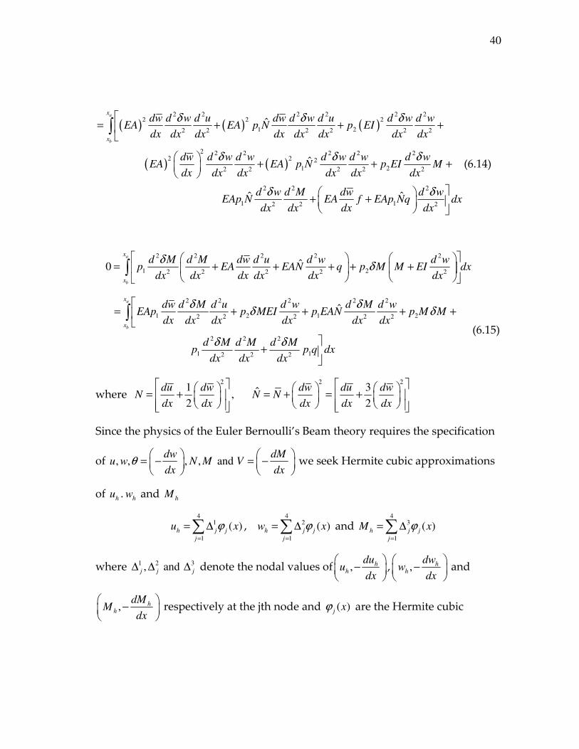
40

( ) ( ) ( )

( ) ( )

2 2 2 2 2 22 2 2

1 22 2 2 2 2 2

2 2 2 2 2 22 2 2

1 22 2 2 2 2

1

ˆ

ˆ

a

b

x

x

dw d w d u dw d w d u d w d wEA EA p N p EI


dw d w d w d w d w d wEA EA p N p EI M

dx dx dx dx dx dx

EAp

δ δ δ

δ δ δ

= + + +

+ + +

∫

2 2 2

12 2 2ˆ ˆd w d M dw d w

N EA f EAp Nq dxdx dx dx dx

δ δ + +

(6.14)

2 2 2 2 2

1 22 2 2 2 2ˆ0

a

b

x

x

d M d M dw d u d w d wp EA EAN q p M M EI dx

dx dx dx dx dx dx

δδ

= + + + + +

∫

2 2 2 2 2

1 2 1 22 2 2 2 2

2 2 2

1 12 2 2

ˆ

a

b

x

x

dw d M d u d w d M d wEAp p MEI p EAN p M M

dx dx dx dx dx dx

d M d M d Mp p q dx

dx dx dx

δ δδ δ

δ δ

= + + + +

+

∫ (6.15)

where 2

1,

2

du dwN

dx dx

= +

2 23ˆ2

dw du dwN N

dx dx dx

= + = +


of , , , , anddw dM

u w N M Vdx dx

θ

= − = −


of hu . hw and hM

4

1

1

( )h j j

j

u xϕ=

= ∆∑ , 4

2

1

( )h j j

j

w xϕ=

= ∆∑ and 4

3

1

( )h j j

j

M xϕ=

= ∆∑

where 1 2 3, andj j j∆ ∆ ∆ denote the nodal values of , hh

duu

dx

−

, , h

h

dww

dx

−

and

, hh

dMM

dx

−


41



1 111 12 13

21 22 23 2 2

31 32 33 3 3

FK K K

K K K F

K K K F

∆ ∆ =

∆

(6.16)

where

( ) ( )22 22 2

2 211

12 2 2 2

a a

b b

x x

j ji iij

x x

d dd ddwK EA dx p EA dx

dx dx dx dx dx

ϕ ϕϕ ϕ = +

∫ ∫

( ) ( )22

212

1 2 2ˆ1

a

b

x

jiij

x

dddwK EA p N dx

dx dx dx

ϕϕ= +∫

2213

1 2 2

a

b

x

jiij

x

dddwK p EA dx

dx dx dx

ϕϕ= ∫

( ) ( )22

221

1 2 2ˆ1

a

b

x

jiij

x

dddwK EA p N dx

dx dx dx

ϕϕ= +∫

( ) ( )2 2 22 2

2 222 2

1 22 2 2 2ˆ

a a

b b

x x

j ji iij

x x

d dd ddwK EA p N dx p EI dx

dx dx dx dx dx

ϕ ϕϕ ϕ = + +

∫ ∫

22 223

1 22 2 2ˆ

a a

b b

x x

ji iij j

x x

dd dK p EAN dx p EI dx

dx dx dx

ϕϕ ϕϕ= +∫ ∫

2231

1 2 2

a

b

x

jiij

x

dddwK p EA dx

dx dx dx

ϕϕ= ∫

( )22 2

232

1 22 2 2ˆ

a a

b b

x x

ji iij j

x x

dd dK p EA N dx p EI dx

dx dx dx

ϕϕ ϕϕ= +∫ ∫

2233

1 22 2

a a

b b

x x

jiij i j

x x

ddK p dx p dx

dx dx

ϕϕϕ ϕ= +∫ ∫

42

2 21

12 2

a

b

x

i ii

x

d ddwF EA f qp dx

dx dx dx

ϕ ϕ = − +

∫

22

1 2ˆ

a

b

x

ii

x

ddwF EAf qp EAN dx

dx dx

ϕ = − + ∫

23

1 2

a

b

x

ii

x

dF p q dx

dx

ϕ= − ∫ (6.17)

From the terms of 33

ijK it is clear that the terms 1p and 2p should be taken such

that 2

2 1 /p p h= , where h is the element length.

6.4 Least-squares Finite Element MODEL 1 for Timoshenko Beam Theory


The equations that arise in connection with the Linear Timoshenko beam

theory are d du

EA fdx dx

− =

S

d dw d dwGAK N q

dx dx dx dxφ

− + − =

0S

d d dwEI GAK

dx dx dx

φφ

− + + =

(6.18)



22

1 2

222 2

2 2 2

( , , )

a

b

x

h hL h h h S

x

h h hS h

d d wJ u w p GAK q

dx dx

d dw d up EI GAK EA f dx

dx dx dx

φφ

φφ

= − + − +

− + + + − −

∫ (6.19)

43





2 2

1 2 2

2 2

2 2

2

2 2

0

a

b

x

h h h hS S

x

h h

h h hS h S h

d d w d d wp GAK GAK q

dx dx dx dx

d u d uEA f EA

dx dx

d w d dwp GAK EI GAK

dx dx dx

δφ δ φ

δ

δ δφδφ φ

= − + − + + +

+ +

+ − +

∫

2

2

hdEI

dx

φ −

(6.20)


of , , , ,dw dM

u w N MandVdx dx

θ

= − = −


of hu . hw and hM

4

1

1

( )h j j

j

u xϕ=

= ∆∑ , 4

2

1

( )h j j

j

w xϕ=

= ∆∑ and 4

3

1

( )h j j

j

M xϕ=

= ∆∑

where 1 2 3,j j jand∆ ∆ ∆ denote the nodal values of , hh

duu

dx

−

, , h

h

dww

dx

−

and

, hh

dMM

dx

−




1 111 12 13

21 22 23 2 2

31 32 33 3 3

FK K K

K K K F

K K K F

∆ ∆ =

∆

(6.21)

where

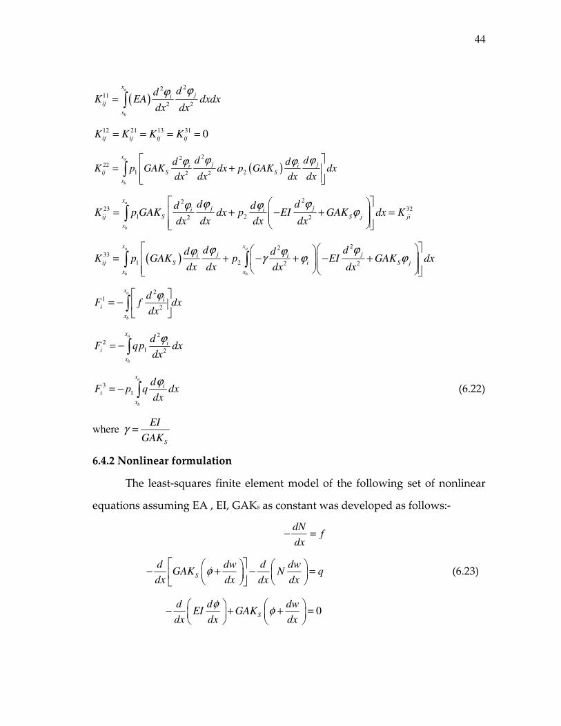
44

( )22

11

2 2

a

b

x

jiij

x

ddK EA dxdx

dx dx

ϕϕ= ∫

12 21 13 31 0ij ij ij ijK K K K= = = =

( )22

22

1 22 2

a

b

x

j ji iij S S

x

d dd dK p GAK dx p GAK dx

dx dx dx dx

ϕ ϕϕ ϕ = +

∫

2223 32

1 22 2

a

b

x

j ji iij S S j ji

x

d dd dK p GAK dx p EI GAK dx K

dx dx dx dx

ϕ ϕϕ ϕϕ

= + − + = ∫

( )22

33

1 2 2 2

a a

b b

x x

j ji iij S i S j

x x

d dd dK p GAK p EI GAK dx

dx dx dx dx

ϕ ϕϕ ϕγ ϕ ϕ

= + − + − + ∫ ∫

21

2

a

b

x

ii

x

dF f dx

dx

ϕ = −

∫

22

1 2

a

b

x

ii

x

dF qp dx

dx

ϕ= −∫

3

1

a

b

x

ii

x

dF p q dx

dx

ϕ= − ∫ (6.22)

where S

EI

GAKγ =


The least-squares finite element model of the following set of nonlinear

equations assuming EA , EI, GAKs as constant was developed as follows:-

dN

fdx

− =

S

d dw d dwGAK N q

dx dx dx dxφ

− + − =

(6.23)

0S

d d dwEI GAK

dx dx dx

φφ

− + + =

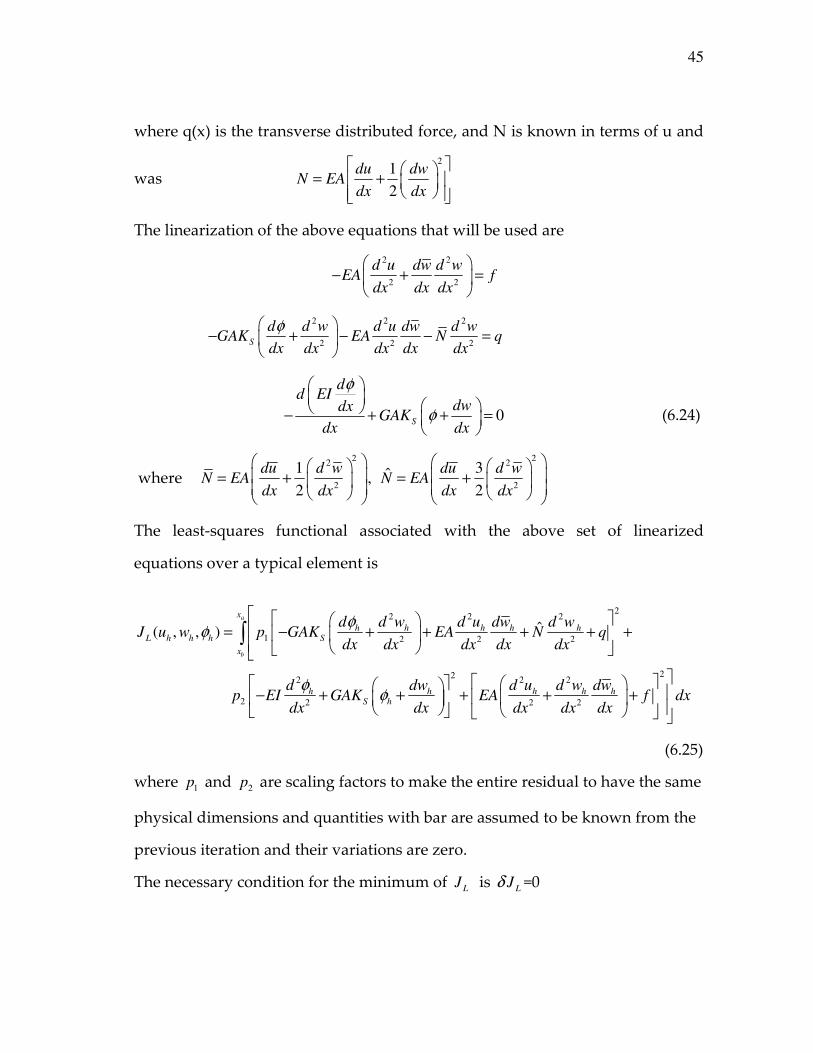
45

where q(x) is the transverse distributed force, and N is known in terms of u and

was 2

1

2

du dwN EA

dx dx

= +

The linearization of the above equations that will be used are

2 2

2 2

d u dw d wEA f

dx dx dx

− + =

2 2 2

2 2 2S

d d w d u dw d wGAK EA N q

dx dx dx dx dx

φ − + − − =

0S

dd EI

dwdxGAK

dx dx

φ

φ

− + + =

(6.24)

where

22

2

1,

2

du d wN EA

dx dx

= +

22

2

3ˆ2

du d wN EA

dx dx

= +



22 2 2

1 2 2 2

222 2 2

2 2 2 2

ˆ( , , )

a

b

x

h h h h hL h h h S

x

h h h h hS h

d d w d u dw d wJ u w p GAK EA N q

dx dx dx dx dx

d dw d u d w dwp EI GAK EA f dx

dx dx dx dx dx

φφ

φφ

= − + + + + +

− + + + + +

∫

(6.25)





46

2 2 2

1 2 2 2

2 2 2

2 2 2

2 2

2 2

ˆ0

ˆ

a

b

x

h h h h hS

x

h h h h hS

h h h

d d w d u dw d wp GAK EA N

dx dx dx dx dx

d d w d u dw d wGAK EA N q

dx dx dx dx dx

d u dw d wEA EA

dx dx dx

δφ δ δ δ

φ

= − + + +

× − + + + + +

+

∫

2 2

2 2

2 2

2 2 2

h h h

h h h hS h S h

d u dw d wf

dx dx dx

d w d dw dp GAK EI GAK EI dx

dx dx dx dx

δ δ

δ δφ φδφ φ

+ + +

+ − + −

(6.26)

The above statement is equivalent to the following three integral statement

2 2 2

2 2 2

2 2 22

1 2 2 2 2

0

ˆ

a

b

x

h

x

h h h h hS

d u d u dw d wEA EA EA f

dx dx dx dx

d d w dw d u d wdw d up EA GAK EA N q dx


δ

φδ

= + + +

− + + + +

∫ (6.27)

2 2

2 2 2

2 2 2 2 2

12 2 2 2 2

2

2

0

ˆ *

a

b

x

h h hS S h

x

h h h h h h hS

h hS

d w d dwp GAK EI GAK

dx dx dx

dw d w d u dw d w d w d wEA EA f p GAK N


d d wGAK

dx dx

δ δφφ

δ δ δ

φ

= − + + +

+ + + +

+

∫

2 2

2 2ˆh h hdw d u d w

EA N q dxdx dx dx

+ + +

(6.28)

2 2 2

1 2 2 2

2 2

2 2 2

ˆ0

a

b

x

h h h h h hS S

x

h h hS h S h

d d d w dw d u d wp GAK GAK EA N q

dx dx dx dx dx dx

d dw dp EI GAK GAK EI dx

dx dx dx

δφ φ

δφ φδφ φ

= − − + + + + +

− + + −

∫ (6.29)

47

where 2

1,

2

du dwN

dx dx

= +

2 23ˆ2

dw du dwN N

dx dx dx

= + = +


of , , , ,dw dM

u w N MandVdx dx

θ

= − = −


of hu . hw and hM

4

1

1

( )h j j

j

u xϕ=

= ∆∑ , 4

2

1

( )h j j

j

w xϕ=

= ∆∑ and 4

3

1

( )h j j

j

M xϕ=

= ∆∑

where 1 2 3,j j jand∆ ∆ ∆ denote the nodal values of , hh

duu

dx

−

, , h

h

dww

dx

−

and

, hh

dMM

dx

−




1 111 12 13

21 22 23 2 2

31 32 33 3 3

FK K K

K K K F

K K K F

∆ ∆ =

∆

(6.30)

where

( ) ( )22 22 2

2 211

12 2 2 2

a a

b b

x x

j ji h iij

x x

d dd dw dK EA dx p EA dx

dx dx dx dx dx

ϕ ϕϕ ϕ = +

∫ ∫

( )( )22

12

1 1 2 2ˆ

a

b

x

jh iij S

x

ddw dK EA EA p N p GAK dx

dx dx dx

ϕϕ= + +∫

2213

1 2 2

a

b

x

jh iij S

x

ddw dK p GAK EA dx

dx dx dx

ϕϕ= ∫

( )( )22

21

1 1 2 2ˆ

a

b

x

jh iij S

x

ddw dK EA EA p N p GAK dx

dx dx dx

ϕϕ= + +∫

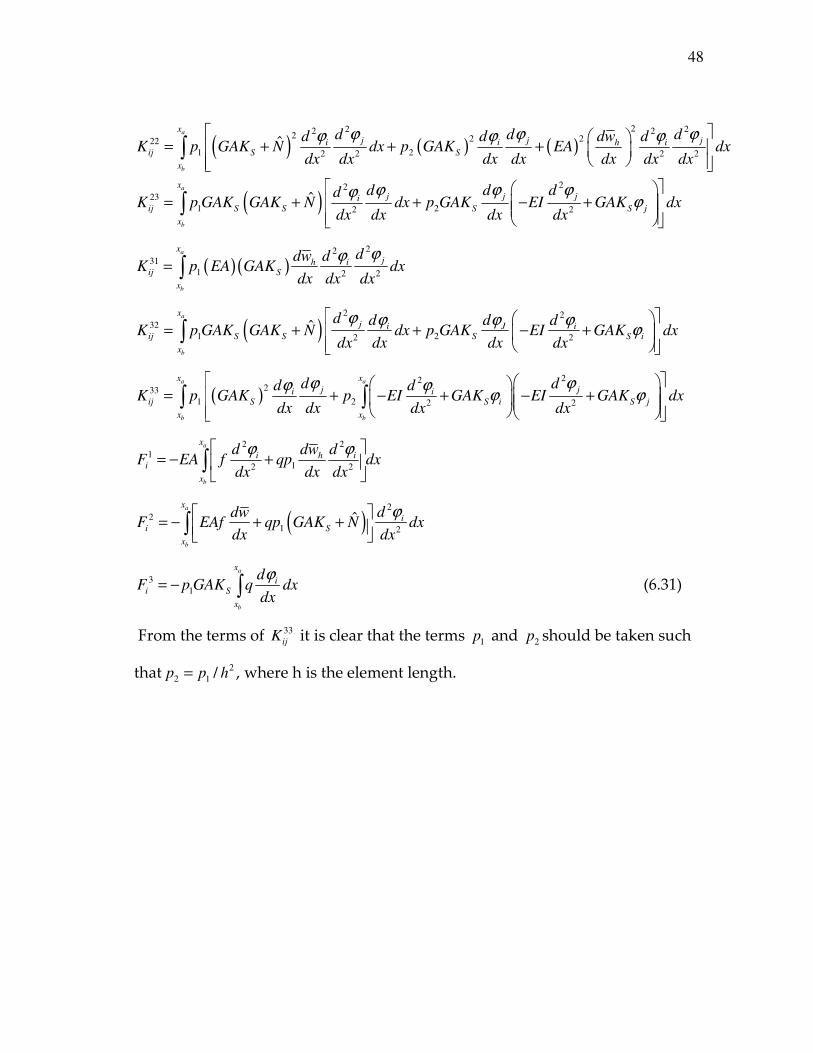
48

( ) ( ) ( )22 22 2

2 2 222

1 22 2 2 2ˆ

a

b

x

j j ji i h iij S S

x

d d dd d dw dK p GAK N dx p GAK EA dx


ϕ ϕ ϕϕ ϕ ϕ = + + +

∫

( )22

23

1 22 2ˆ

a

b

x

j j jiij S S S S j

x

d d ddK p GAK GAK N dx p GAK EI GAK dx

dx dx dx dx

ϕ ϕ ϕϕϕ

= + + − + ∫

( )( )22

31

1 2 2

a

b

x

jh iij S

x

ddw dK p EA GAK dx

dx dx dx

ϕϕ= ∫

( )2 2

32

1 22 2ˆ

a

b

x

j i J iij S S S S i

x

d d d dK p GAK GAK N dx p GAK EI GAK dx

dx dx dx dx

ϕ ϕ ϕ ϕϕ

= + + − +

∫

( )22

233

1 2 2 2

a a

b b

x x

j ji iij S S i S j

x x

d dd dK p GAK p EI GAK EI GAK dx

dx dx dx dx

ϕ ϕϕ ϕϕ ϕ

= + − + − + ∫ ∫

2 21

12 2

a

b

x

i h ii

x

d dw dF EA f qp dx

dx dx dx

ϕ ϕ = − +

∫

( )2

2

1 2ˆ

a

b

x

ii S

x

ddwF EAf qp GAK N dx

dx dx

ϕ = − + + ∫

3

1

a

b

x

ii S

x

dF p GAK q dx

dx

ϕ= − ∫ (6.31)

From the terms of 33

ijK it is clear that the terms 1p and 2p should be taken such

that 2

2 1 /p p h= , where h is the element length.

49

6.5 Least-squares Finite Element MODEL 2 for Euler-Bernoulli Beam Theory


Consider the four first-order governing equations

0, 0

0, 0

0, 0

dN N duf

dx EA dx

dV dwkw q

dx dx

M d dMV

b dx dx

θ

θ

− − = − =

− + − = + =

− = − + =

(6.32)

here b=EI

The least-squares functional associated with the above six equations over a

typical element is

2 2 2 2

2

2 2

( , ,...)

b

a

x

h h h h hh h h h

x

h h hh

dN N du dV dwJ u w f kw q

dx EA dx dx dx

M d dMV dx

b dx dx

θ

θ

= + + − + − + − + + +

− + − +

∫

(6.33)

Here b=EI and the necessary condition for minimum of 2J is

0b

a

x

h h h h h h

x

h h h hh h h h

h h h h h hh h

d N dN N d u N duf

dx dx EA dx EA dx

d V dV d w dwk w kw q

dx dx dx dx

M d M d d M dMV V

EI dx EI dx dx dx

δ δ δ

δ δδ δθ θ

δ δθ θ δδ

= + + − − +

− + − + − + + + +

− − + − + − +

∫

dx

(6.34)

The four statements associated with the statement in the above equations are:

50

0

0

0

0

b

a

b

a

b

a

x

h h h

x

x

h h hh h h

x

x

h h h hh h

x

h h h h h

d u N dudx

dx EA dx

dV d w dwk w kw q dx

dx dx dx

dw d M ddx

dx dx EI dx

d N dN N N duf

dx dx EA EA dx

δ

δδ θ

δθ θδθ θ

δ δ

= − −

= − + − + +

= + − −

= + + −

∫

∫

∫

0

0

b

a

b

a

b

a

x

x

x

h h h h hh

x

x

h h hh h h

x

dx

M M d d M dMV dx

b b dx dx dx

d V dV dMkw q V V dx

dx dx dx

δ θ δ

δδ

= − + − +

= − − + − − − +

∫

∫

∫

(6.35)

In this model, all physical variables that enter the specification of the boundary

conditions appear as unknowns. Hence they are all approximated by Lagrange

interpolation functions. Let,

( ) ( ) ( )

( ) ( ) ( )

1 1 1

1 1 1

, , ,

, ,

m m m

h j j h j j h j j

j j j

m m m

h j j h j j h j j

j j j

u u x w w x x

N N x M M x V V x

ψ ψ θ θ ψ

ψ ψ ψ

= = =

= = =

= = =

= = =

∑ ∑ ∑

∑ ∑ ∑

Where , , and j j j jw M Vθ denote the nodal values of , , and h h h hw M Vθ respectively

at the jth node. Thus we obtain the following finite element model

11 12 13 14 15 16

21 22 23 24 25 26

31 32 33 34 35 36

41 42 43 44

51 52 53

61 62 63

K K K K K K

K K K K K K

K K K K K K

K K K K

K K K

K K K

1

2

3

45 46 4

54 55 56 5

64 65 66 6

Fu

Fw

F

NK K F

MK K K F

VK K K F

θ

=

(6.36)

51

where

11

14

22 2

23

26

32

33

35

1

1

b

a

b

a

b

a

b

a

b

a

b

a

b

a

x

jiij

x

x

iij j

x

x

j jiij i

x

x

iij j

x

x

j

ij i

x

x

j

ij i

x

x

jiij j i

x

iij j

x

ddK dx

dx dx

dK dx

EA dx

d ddK k dx

dx dx dx

dK dx

dx

dK k dx

dx

dK dx

dx

ddK dx

dx dx

dK

EI dx

ψψ

ψψ

ψ ψψψ

ψψ

ψψ

ψψ

ψψψ ψ

ψψ

=

= −

= +

=

= −

=

= +

= −

∫

∫

∫

∫

∫

∫

∫

( )

( )

41

44

2

53

55

2

56

62

1

1

1

1

b

a

b

a

b

a

b

a

b

a

b

a

b

a

x

x

j

ij i

x

x

jiij j i

x

x

j

ij i

x

x

jiij j i

x

x

iij j

x

x

iij j

x

dx

dK dx

EA dx

ddK dx

dx dxEA

dK dx

EI dx

ddK dx

dx dxEI

dK dx

dx

dK k dx

dx

ψψ

ψψψ ψ

ψψ

ψψψ ψ

ψψ

ψψ

= −

= +

= −

= +

= −

= −

∫

∫

∫

∫

∫

∫

∫

52

65

66

2

4

6

b

a

b

a

b

a

b

a

b

a

x

j

ij i

x

x

jiij j i

x

x

i i

x

x

ii

x

x

ii

x

dK dx

dx

ddK dx

dx dx

F kq dx

dF f dx

dx

dF q dx

dx

ψψ

ψψψ ψ

ψ

ψ

ψ

= −

= +

=

= −

= −

∫

∫

∫

∫

∫

(6.37)


Here consider the first-order equations

( )

2

0, 0

0, 0

0, 0

dN N du dwf

dx EA dx dx

dV d dwN q

dx dx dx

M d dMV

EI dx dx

θ θ

θ

− − = − + =

− + − = + =

− = − + =

(6.38)


typical element is

( )

22 2 2

2

2 2 2

( , ,...)b

a

x

h h h h hh h

x

h h h hh h

dN N du dw dV dJ u w f N q

dx EA dx dx dx dx

dw M d dMV dx

dx EI dx dx

θ

θθ

= + + − + + − + − +

+ + − + − +

∫

(6.39)

The necessary condition for minimum of 2J is

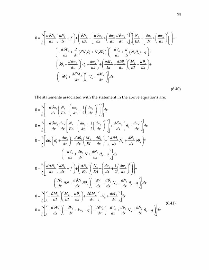
53

( ) ( )

2

0b

a

x

h h h h h h h h h

x

h hh h h h h h

h h hh h

d N dN N d u dw d w N du dwf

dx dx EA dx dx dx EA dx dx

d V dVd dN N N q

dx dx dx dx

d w dw M

dx dx EI

δ δ δ δ

δδ θ δθ θ

δ δδθ θ

= + + − + − + +

− + + − + − +

+ + +

∫

h h h

h hh h

d M d

dx EI dx

d M dMV V dx

dx dx

δθ θ

δδ

− − +

− + − +

(6.40)

The statements associated with the statement in the above equations are:

2

2

10

2

10

2

0

b

a

b

a

x

h h h h

x

x

h h h h h h hh

x

h h h hh h

d u N du dwdx

dx EA dx dx

d w dw N du dw d w dwdx

dx dx EA dx dx dx dx

dw d M d d

dx dx EI dx

δ

δ δθ

δθ θδθ θ

= − − +

= − − + + +

= + − − +

∫

∫

2

*

10

2

b

a

b

a

x

h hh h

x

h h hh

x

h h h h h h

x

h h hh h h

dNN

dx dx

dV d dNN q dx

dx dx dx

d N dN N N du dwf

dx dx EA EA dx dx

d d dNd N dVN N q

dx dx dx dx dx

δθδθ

θθ

δ δ

θ θδδ δθ θ

+

− + + −

= + + − + +

+ − + + −

∫

∫

0

0

b

a

b

a

x

h h h h hh

x

x

h h h h h hh h h

x

dx

M M d d M dMV dx

EI EI dx dx dx

d V dV d V dV d dNkw q N q dx

dx dx dx dx dx dx

δ θ δ

δ δ θθ

= − − + − +

= − − + − − − + + −

∫

∫

(6.41)

54




( ) ( ) ( )

( ) ( ) ( )

1 1 1

1 1 1

, , ,

, ,

m m m

h j j h j j h j j

j j j

m m m

h j j h j j h j j

j j j

u u x w w x x

N N x M M x V V x

ψ ψ θ θ ψ

ψ ψ ψ

= = =

= = =

= = =

= = =

∑ ∑ ∑

∑ ∑ ∑

Where , , and j j j jw M Vθ denote the nodal values of , , and h h h hw M Vθ respectively


11 12 13 14 15 16

21 22 23 24 25 26

31 32 33 34 35 36

41 42 43 44

51 52 53

61 62 63

K K K K K K

K K K K K K

K K K K K K

K K K K

K K K

K K K

1

2

3

45 46 4

54 55 56 5

64 65 66 6

Fu

Fw

F

NK K F

MK K K F

VK K K F

θ

=

(6.42)

where

11 12

14 21

2

22

23 32

1,

2

1,

1

2

,

b b

a a

b b

a a

b

a

b b

a a

x x

j ji iij ij

x x

x x

ji iij j ij

x x

x

j ji iij

x

x x

jiij j ij i

x x

d dd ddwK dx K dx

dx dx dx dx dx

dd ddwK dx K dx

EA dx dx dx dx

d dd d dwK dx

dx dx dx dx dx

ddK dx K d

dx dx

ψ ψψ ψ

ψψ ψψ

ψ ψψ ψ

ψψψ ψ

= =

= − =

= +

= =

∫ ∫

∫ ∫

∫

∫ ∫ x

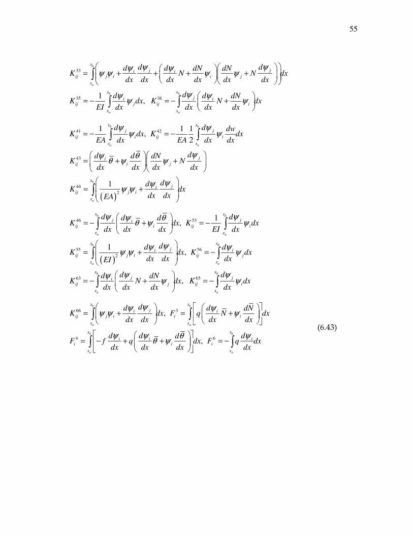
55

33

35 361,

b

a

b b

a a

x

j ji iij j i i j

x

x x

ji iij j ij i

x x

d dd d dN dNK N N dx

dx dx dx dx dx dx

dd d dNK dx K N dx

EI dx dx dx dx

ψ ψψ ψψ ψ ψ ψ

ψψ ψψ ψ

= + + + +

= − = − +

∫

∫ ∫

( )

41 42

43

44

2

1 1 1,

2

1

b b

a a

b

a

x x

j j

ij i ij i

x x

jiij i j

x

jiij j i

x

d d dwK dx K dx

EA dx EA dx dx

dd d dNK N

dx dx dx dx

ddK dx

dx dxEA

ψ ψψ ψ

ψψ θθ ψ ψ

ψψψ ψ

= − = −

= + +

= +

∫ ∫

∫

( )

46 53

55 56

2

63 65

1,

1,

,

b b

a a

b b

a a

b b

a a

x x

j jiij i ij i

x x

x x

ji iij j i ij j

x x

x x

j jiij j ij i

x x

d dd dK dx K dx

dx dx dx EI dx

dd dK dx K dx

dx dx dxEI

d dd dNK N dx K dx

dx dx dx dx

ψ ψψ θθ ψ ψ

ψψ ψψ ψ ψ

ψ ψψψ ψ

= − + = −

= + = −

= − + = −

∫ ∫

∫ ∫

∫ ∫

66 3

4 6

,

,

b b

a a

b b

a a

x x

ji iij j i i i

x x

x x

i i ii i i

x x

dd d dNK dx F q N dx

dx dx dx dx

d d ddF f q dx F q dx

dx dx dx dx

ψψ ψψ ψ ψ

ψ ψ ψθθ ψ

= + = +

= − + + = −

∫ ∫

∫ ∫

(6.43)

56

6.6 Least-squares Finite Element MODEL 2 for Timoshenko Beam Theory


Consider the first-order governing equations

0, 0

0,

0, 0

dN N duf

dx EA dx

dV dwq V GAK

dx dx

M d dMV

EI dx dx

φ

θ

− − = − =

− − = = +

− = − + =

(6.44)


typical element is

22 2 2

2

2 2

( , ,...)b

a

x

h h h h hh h h h

x

h h hh

dN N du dV dwJ u w f q V GAK

dx EA dx dx dx

M d dMV dx

EI dx dx

φ

θ

= + + − + − − + − + +

− + − +

∫

(6.45)


0b

a

x

h h h h h h

x

h h h hh h h h

h h h h hh

d N dN N d u N duf

dx dx EA dx EA dx

d V dV d w dwq V GAK V GAK

dx dx dx dx

M d M d d MV

EI dx EI dx dx

δ δ δ

δ δδ δφ φ

δ δθ θ δδ

= + + − − +

+ + − + − + +

− − + − + −

∫

hh

dMV dx

dx

+

(6.46)

57


0

0

0

0

b

a

b

a

b

a

b

a

x

h h h

x

x

h h hh

x

x

h h h h hh h

x

x

h h h h h

x

d u N dudx

dx EA dx

d w V dwdx

dx GAK dx

V dw d M ddx

GAK dx dx EI dx

d N dN N N duf

dx dx EA EA dx

δ

δφ

δθ θδθ φ

δ δ

= − −

= − −

= − − − −

= + + −

∫

∫

∫

∫

0

0

b

a

b

a

x

h h h h hh

x

x

h h h h h hh h h

x

dx

M M d d M dMV dx

EI EI dx dx dx

d V dV dM V V dwq V V dx

dx dx dx GAK GAK dx

δ θ δ

δ δδ φ

= − + − +

= + − − + + − −

∫

∫

(6.47)




( ) ( ) ( )

( ) ( ) ( )

1 1 1

1 1 1

, , ,

, ,

m m m

h j j h j j h j j

j j j

m m m

h j j h j j h j j

j j j

u u x w w x x

N N x M M x V V x

ψ ψ φ φ ψ

ψ ψ ψ

= = =

= = =

= = =

= = =

∑ ∑ ∑

∑ ∑ ∑

where , , and j j j jw M Vθ denote the nodal values of , , and h h h hw M Vθ respectively


58

11 12 13 14 15 16

21 22 23 24 25 26

31 32 33 34 35 36

41 42 43 44

51 52 53

61 62 63

K K K K K K

K K K K K K

K K K K K K

K K K K

K K K

K K K

1

2

3

45 46 4

54 55 56 5

64 65 66 6

Fu

Fw

F

NK K F

MK K K F

VK K K F

φ

=

(6.48)

where

11 14 22

23 26 32

33 35

1, ,

1, ,

1,

b b b

a a a

b b b

a a a

b

a a

x x x

j ji i iij ij j ij

x x x

x x x

j jiij j ij i ij i

x x x

x

ji iij j i ij j

x x

d dd d dK dx K dx K dx

dx dx EA dx dx dx

d ddK dx K dx K dx

dx GAK dx dx

dd dK dx K

dx dx EI dx

ψ ψψ ψ ψψ

ψ ψψψ ψ ψ

ψψ ψψ ψ ψ

= = − =

= = = −

= − + = −

∫ ∫ ∫

∫ ∫ ∫

∫

( )

( )

41 44

2

53 55

2

1 1,

1 1,

b

b b

a a

b b

a a

x

x x

j jiij i ij j i

x x

x x

j jiij i ij j i

x x

dx

d ddK dx K dx

EA dx dx dxEA

d ddK dx K dx

EI dx dx dxEI

ψ ψψψ ψ ψ

ψ ψψψ ψ ψ

= − = +

= − = +

∫

∫ ∫

∫ ∫

56 62 63

65 66

4 6

, ,

,

,

b b b

a a a

b b

a a

b b

a a

x x x

i iij j ij j ij i j

x x x

x x

j jiij i ij j i

x x

x x

i ii i

x x

d dK dx K dx K dx

dx dx

d ddK dx K dx

dx dx dx

d dF f dx F q dx

dx dx

ψ ψψ ψ ψ ψ

ψ ψψψ ψ ψ

ψ ψ

= − = − = −

= − = +

= − = −

∫ ∫ ∫

∫ ∫

∫ ∫

(6.49)


Here consider the first-order equations

59

2

0, 0

0, 0

0, 0

dN N du dwf

dx EA dx dx

dV d V V dwN q

dx dx GAK GAK dx

M d dMV

EI dx dx

φ φ

θ

− − = − + =

− + − − = − + =

− = − + =

(6.50)


typical element is

22 2

2

2

2 2 2

( , ,...)b

a

x

h h h hh h

x

h h hh

dN N du dwJ u w f

dx EA dx dx

dV d VN q

dx dx GAK

M d dMV dwV dx

GAK dx EI dx dx

φ

θφ

= + + − + +

− + − − +

− + + − + − +

∫

(6.51)


2

0b

a

x

h h h h h h h h h

x

h

d N dN N d u dw d w N du dwf

dx dx EA dx dx dx EA dx dx

d V d V dV d VN N q

dx dx GAK dx dx GAK

d wV

GAK d

δ δ δ δ

δδ φ φ

δδδφ

= + + − + − + +

− + − − + − − +

− +

∫

h h h h h

h hh h

dw M d M dV

x GAK dx EI dx EI dx

d M dMV V dx

dx dx

δ δθ θφ

δδ

− + + − − +

− + − +

(6.52)


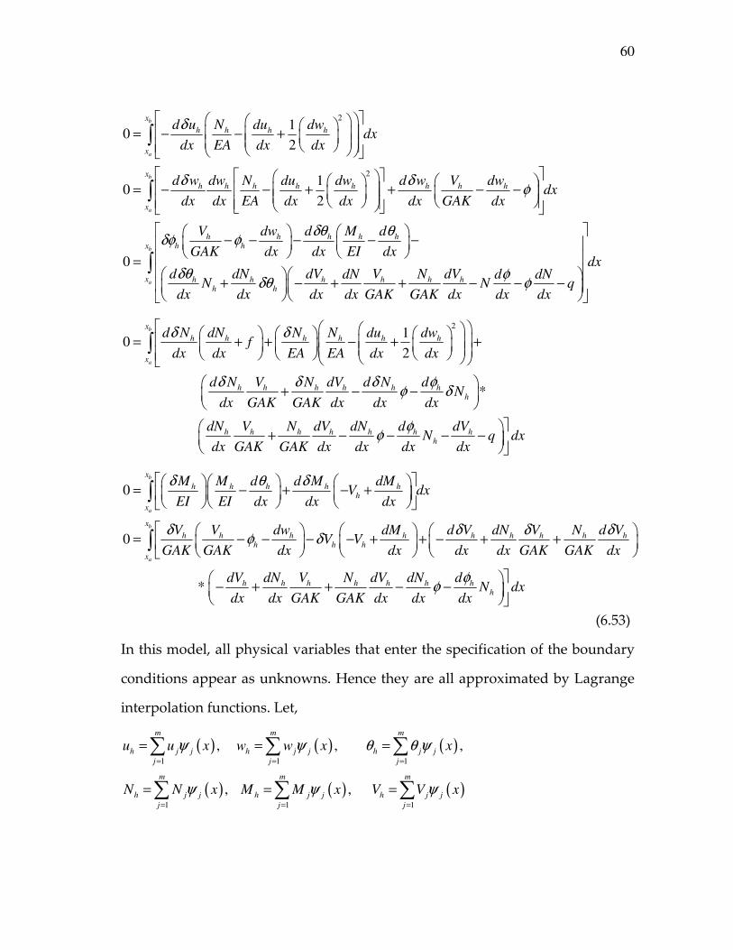
60

2

2

10

2

10

2

0

b

a

b

a

x

h h h h

x

x

h h h h h h h h

x

h h h hh h

d u N du dwdx

dx EA dx dx

d w dw N du dw d w V dwdx

dx dx EA dx dx dx GAK dx

V dw d M d

GAK dx dx EI

δ

δ δφ

δθ θδφ φ

= − − +

= − − + + − −

− − − −

=

∫

∫

b

a

hx

x h h h h h hh h

dxdx

d dN dV V N dVdN d dNN N q

dx dx dx dx GAK GAK dx dx dx

δθ φδθ φ

−

+ − + + − − −

∫

21

02

*

b

a

x

h h h h h h

x

h h h h h hh

h h h h h h hh

d N dN N N du dwf

dx dx EA EA dx dx

d N V N dV d N dN

dx GAK GAK dx dx dx

dN V N dV dN d dVN q dx

dx GAK GAK dx dx dx dx

δ δ

δ δ δ φφ δ

φφ

= + + − + +

+ − −

+ − − − −

∫

0

0

*

b

a

b

a

x

h h h h hh

x

x

h h h h h h h h hh h h

x

h h h h h h h

M M d d M dMV dx

EI EI dx dx dx

V V dw dM d V dN V N d VV V

GAK GAK dx dx dx dx GAK GAK dx

dV dN V N dV dN dN

dx dx GAK GAK dx dx dx

δ θ δ

δ δ δ δφ δ

φφ

= − + − +

= − − − − + + − + +

− + + − −

∫

∫

h dx

(6.53)




( ) ( ) ( )

( ) ( ) ( )

1 1 1

1 1 1

, , ,

, ,

m m m

h j j h j j h j j

j j j

m m m

h j j h j j h j j

j j j

u u x w w x x

N N x M M x V V x

ψ ψ θ θ ψ

ψ ψ ψ

= = =

= = =

= = =

= = =

∑ ∑ ∑

∑ ∑ ∑

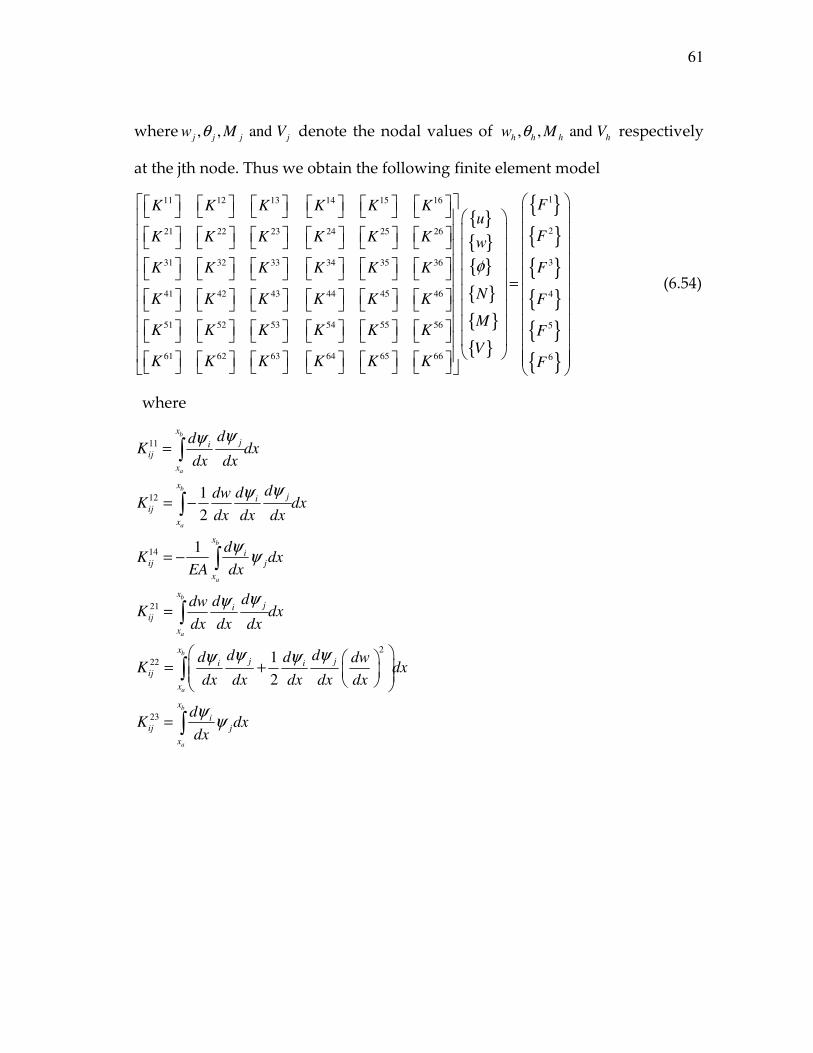
61

where , , and j j j jw M Vθ denote the nodal values of , , and h h h hw M Vθ respectively


11 12 13 14 15 16

21 22 23 24 25 26

31 32 33 34 35 36

41 42 43 44

51 52 53

61 62 63

K K K K K K

K K K K K K

K K K K K K

K K K K

K K K

K K K

1

2

3

45 46 4

54 55 56 5

64 65 66 6

Fu

Fw

F

NK K F

MK K K F

VK K K F

φ

=

(6.54)

where

11

12

14

21

2

22

23

1

2

1

1

2

b

a

b

a

b

a

b

a

b

a

b

a

x

jiij

x

x

jiij

x

x

iij j

x

x

jiij

x

x

j ji iij

x

x

iij j

x

ddK dx

dx dx

dddwK dx

dx dx dx

dK dx

EA dx

dddwK dx

dx dx dx

d dd d dwK dx

dx dx dx dx dx

dK dx

dx

ψψ

ψψ

ψψ

ψψ

ψ ψψ ψ

ψψ

=

= −

= −

=

= +

=

∫

∫

∫

∫

∫

∫

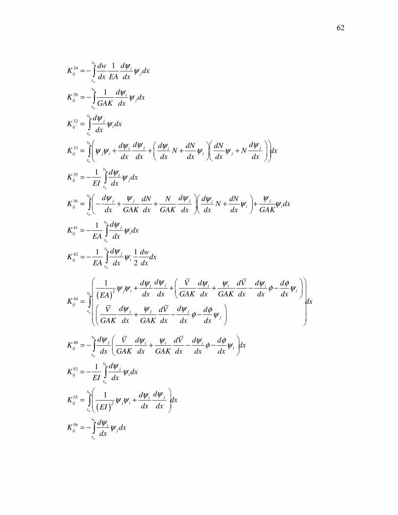
62

24

26

32

33

35

36

1

1

1

b

a

b

a

b

a

b

a

b

a

x

iij j

x

x

iij j

x

x

j

ij i

x

x

j ji iij j i i j

x

x

iij j

x

j j

ij

ddwK dx

dx EA dx

dK dx

GAK dx

dK dx

dx

d dd d dN dNK N N dx

dx dx dx dx dx dx

dK dx

EI dx

d ddN NK

dx GAK dx GAK

ψψ

ψψ

ψψ

ψ ψψ ψψ ψ ψ ψ

ψψ

ψ ψ

= −

= −

=

= + + + +

= −

= − + +

∫

∫

∫

∫

∫

41

42

1

1 1

2

b

a

b

a

b

a

x

j jii i

x

x

j

ij i

x

x

j

ij i

x

d dNN dx

dx dx dx GAK

dK dx

EA dx

d dwK dx

EA dx dx

ψ ψψψ ψ

ψψ

ψψ

+ +

= −

= −

∫

∫

∫

( )2

44

1

b

a

ji i i ij i ix

ij

x j j j

j

dd d dV dV d

dx dx GAK dx GAK dx dx dxEAK dx

d dV dV d

GAK dx GAK dx dx dx

ψψ ψ ψ ψ φψ ψ φ ψ

ψ ψ ψ φφ ψ

+ + + − −

=

+ − −

∫

( )

46

53

55

2

56

1

1

b

a

b

a

b

a

b

a

x

j i i iij i

x

x

j

ij i

x

x

jiij j i

x

x

iij j

x

d d dV dV dK dx

dx GAK dx GAK dx dx dx

dK dx

EI dx

ddK dx

dx dxEI

dK dx

dx

ψ ψ ψ ψ φφ ψ

ψψ

ψψψ ψ

ψψ

= − + − −

= −

= +

= −

∫

∫

∫

∫

63

( )

62

63

65

66

2

1

b

a

b

a

b

a

b

a

x

j iij

x

x

i j ji i iij j

x

x

j

ij i

x

x

i i iij j i j i

x

j j

dK

dx GAK

dd d ddN N dNK N dx

GAK dx dx dx GAK dx dx dx

dK dx

dx

d d ddN NK

dx dx dx GAK dxGAK

d dN

dx dx G

ψ ψ

ψ ψ ψψ ψ ψψ

ψψ

ψ ψ ψψ ψ ψ ψ

ψ ψ

= −

= − + − + + +

= −

= + + − + +

− +

∫

∫

∫

∫

4

3

6

b

a

b

a

b

a

j

x

i i i ii i

x

x

ii i

x

x

ii

x

dNdx

AK GAK dx

d d dV dV dF f q dx

dx GAK dx GAK dx dx dx

d dNF q N dx

dx dx

dF q dx

dx

ψ

ψ ψ ψ ψ φφ ψ

ψψ

ψ

+

= − + + − −

= − +

= −

∫

∫

∫ (6.55)

64

7. SOLUTION APPROACH

Different methods to develop the finite element model have been

discussed so far. An interaction of local and global coordinates is used to obtain

the results. The element coefficient matrices are assembled. During assembly the

stiffness contributed by the adjacent element to the common coordinates will be

doubled. Different boundary conditions are imposed and the value of F and

u are computed. The elemental values of primary variables will be considered

during the next cycle of iteration. Convergence is reached when the error is less

than the tolerance value. For the practical purposes the absolute error should be

small to at lower computational expense. The rate at which certain results

approach the exact solution is very important.

7.1 Solution Procedures

There are two different iterative methods discussed here

(1) Direct iteration procedure (2) Newton Raphson iteration procedure

7.1.1 Direct iteration procedure

Here the solution of the coefficient matrix is computed using the known

value from the previous solution of the (r-1) th iteration. The solution for the rth

iteration can be determined from the following equation

( )( ) ( )( ) 1 1

or r r r r

K F K F− − ∆ ∆ = ∆ ∆ =

Thus the initial guess vector should satisfy the boundary conditions.

7.2.2 Newton-Raphson iteration procedure

Consider the following equation,

[ ] 0R K U F≡ − = (7.1)

where R is the residual vector. We expand R in the Taylor’s series as

65

( ) ( )( )

( )

( )

( )( )

( )( ) ( )( )

1

1

1

1

1 1

. .......

.

.

r

r

r

r

r r

RR U R U U

U

RU R U

U

T U U R U

δ

δ

δ

−

−

−

−

− −

∂= + + ∂

∂= − ∂

= −

(7.2)

Here T is the tangent matrix which is equal to,

( )( )

( )

( )( ) ( )1 1

1 1

r re

r r i

e

i

R RT U or T U

U U

− −

− − ∂ ∂= = ∂ ∂

(7.3)

For rth iteration we have, ( ) 1r r

δ−

∆ = ∆ + ∆

Thus we can write,

( )1

2

1

2 41 1 2 2

1 1

2 41 2

1 1

r

iij

j

i ip p i

p

ip p iP P i

p P

ip p iP P i

p P

RT

R K F

K K F

K u K F

ααβ

β

α αγ γ α

γ

α α α

α α α

−

=

= =

= =

∂= ∂∆

= ∆ −

= ∆ + ∆ −

= + ∆ −

∑∑

∑ ∑

∑ ∑

(7.4)

( )

( ) ( )

12

1

2 41 2

1 1

r

iij ip p i

pj j

ij ip p iP P

p Pj j

RT K F

K K u K u

ααβ αγ γ α

β βγ

αβ α α

β β

−

=

= =

∂ ∂= = ∆ − ∂∆ ∂∆

∂ ∂= + +

∂∆ ∂∆

∑∑

∑ ∑ (7.5)

The coefficients of tangent matrices for EBT conventional weighted residual

method can be found by substituting the stiffness coefficients in from equations

(4.13) in equation (7.5).

66

11 11

21 21

12 12

2

22 22 0 0

2

1

2

b

a

ij ij

Ji Ji

iJ iJ

x

J IIJ IJ xx

x

T K

T K

T K

dw du d dT K A dx

dx dx dx dx

φ φ

=

=

=

= + +

∫

(7.6)

Similarly for TBT conventional weighted residual method we get the following

coefficients of tangent matrices.

11 11

(2)(1)12 12 120

13 13

12

2

b

a

ij ij

x

jiij ij xx ij

x

ij ij

T K

ddw dT K A dx K

dx dx dx

T K

ψψ

=

= + =

=

∫

21 21

2 (2)(2)22 22 0 0

23 23

31 31

32 32

33 33

1

2

b

a

ij ij

x

jiij ij xx

x

ij ij

ij ij

ij ij

ij ij

T K

ddw du dT K A dx

dx dx dx dx

T K

T K

T K

T K

ψψ

=

= + +

=

=

=

=

∫

(7.7)

A flowchart to explain the logic behind the computer implementation is shown

in Figure 7.1.

67

Figure 7.1. A computer implementation flowchart

68

8. DISCUSSION OF NUMERICAL RESULTS

The following example is considered for EBT and TBT model for

conventional weak form and least-squares MODEL1 and MODEL2.

8.1. Example

Consider a linear elastic column which is subjected to a uniformly

distributed load q= 10 in 10 load steps .Let L denote the length of the column, EI

denote the flexural rigidity of the beam where E is the Young modulus and I is

the moment of inertia of the cross section of the column, w(x) denote the

deflection function, M denote the bending moment and V denote the shear

force. Here calculations have been made with the following data E=30msi,

L=100 in, area (A) =1x1 in2. tolerance =0.001 maximum number of iterations=30

Boundary conditions: 1) both ends hinged 2) both ends clamped 3) both ends

pinned ( see Reddy [3]). The beam is analyzed for 4,8, and 32 elements.

8.2. Results

For beam with both ends hinged.

1) 4 ELEMENTS

(A) Conventional weighted residual method (Table 8.1)

Table 8.1: Comparison of displacements in EBT and TBT for hinged-hinged

beam

EBT TBT

NODE X U W DW/DX U W PHI

1 0.000 0.000 0.000 -0.017 0.000 0.000 -0.016

2 12.500 0.000 0.202 -0.015 0.000 0.197 -0.015

69

Table 8.1 continued.

EBT TBT


3 25.000 0.000 0.371 -0.011 0.000 0.361 -0.011

4 37.500 0.000 0.482 -0.006 0.000 0.470 -0.006

5 50.000 0.000 0.521 0.000 0.000 0.508 0.000

(B) a) Least-squares finite element MODEL1 –EBT (Table 8.2)

Table 8.2: Comparison of displacements and forces in EBT for hinged-hinged

beam

NODE X U DU/DX W DW/DX M DM/DX

1 0.0000 0.0000 0.0000 0.0000 -0.0166 0.0000 -49.9310

2 12.5000 0.0000 0.0000 0.2020 -0.0152 546.1200 -37.4480

3 25.0000 0.0000 0.0000 0.3706 -0.0114 936.2000 -24.9650

4 37.5000 0.0000 0.0000 0.4815 -0.0061 1170.2000 -12.4830

5 50.0000 0.0000 0.0000 0.5201 0.0000 1248.3000 0.0000

(B) b) Least-squares finite element MODEL1 –TBT (Table 8.3)

Table 8.3: Comparison of displacements and forces in TBT for hinged-hinged

beam


1 0.0000 0.0000 0.0000 0.0000 -0.0152 -0.0152 0.0000

2 12.5000 0.0000 0.0000 0.1844 -0.0139 -0.0139 -0.0002

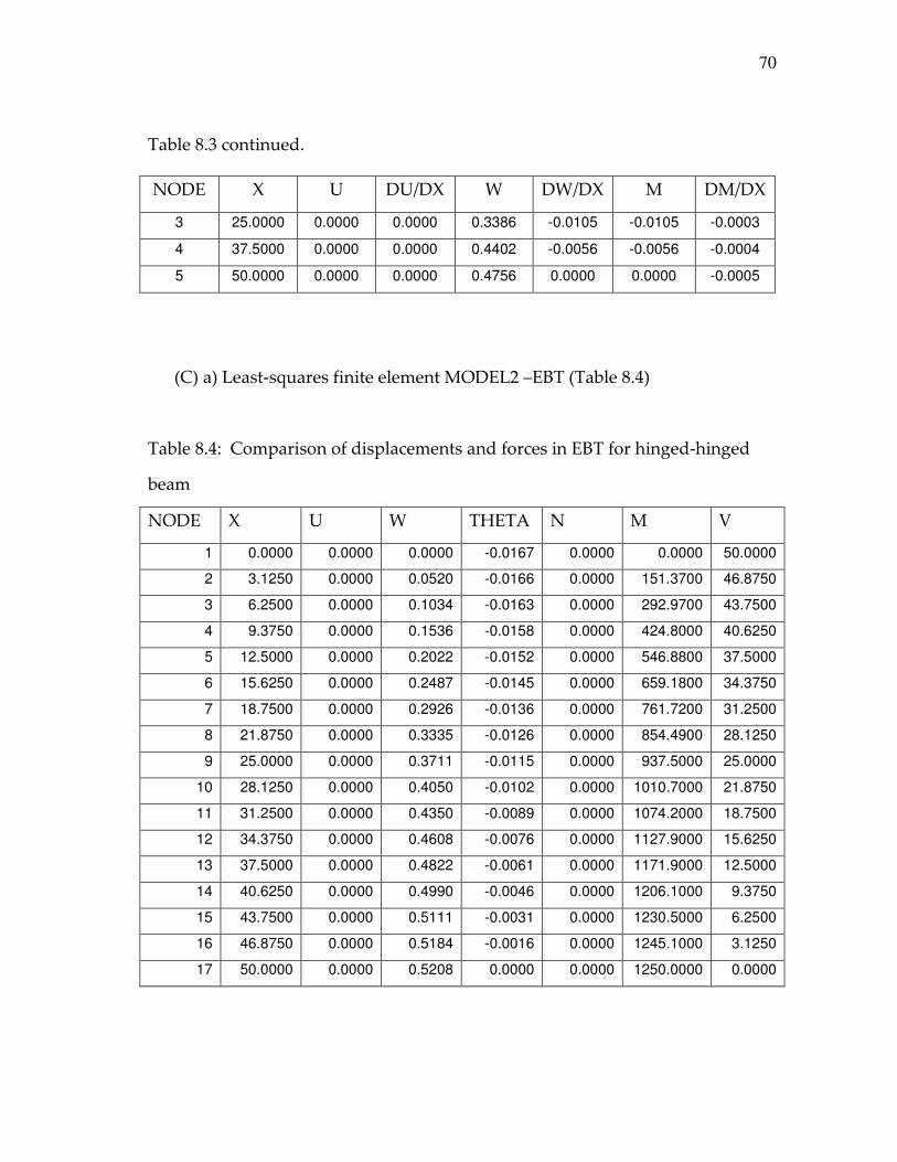
70



3 25.0000 0.0000 0.0000 0.3386 -0.0105 -0.0105 -0.0003

4 37.5000 0.0000 0.0000 0.4402 -0.0056 -0.0056 -0.0004

5 50.0000 0.0000 0.0000 0.4756 0.0000 0.0000 -0.0005

(C) a) Least-squares finite element MODEL2 –EBT (Table 8.4)

Table 8.4: Comparison of displacements and forces in EBT for hinged-hinged

beam

NODE X U W THETA N M V

1 0.0000 0.0000 0.0000 -0.0167 0.0000 0.0000 50.0000

2 3.1250 0.0000 0.0520 -0.0166 0.0000 151.3700 46.8750

3 6.2500 0.0000 0.1034 -0.0163 0.0000 292.9700 43.7500

4 9.3750 0.0000 0.1536 -0.0158 0.0000 424.8000 40.6250

5 12.5000 0.0000 0.2022 -0.0152 0.0000 546.8800 37.5000

6 15.6250 0.0000 0.2487 -0.0145 0.0000 659.1800 34.3750

7 18.7500 0.0000 0.2926 -0.0136 0.0000 761.7200 31.2500

8 21.8750 0.0000 0.3335 -0.0126 0.0000 854.4900 28.1250

9 25.0000 0.0000 0.3711 -0.0115 0.0000 937.5000 25.0000

10 28.1250 0.0000 0.4050 -0.0102 0.0000 1010.7000 21.8750

11 31.2500 0.0000 0.4350 -0.0089 0.0000 1074.2000 18.7500

12 34.3750 0.0000 0.4608 -0.0076 0.0000 1127.9000 15.6250

13 37.5000 0.0000 0.4822 -0.0061 0.0000 1171.9000 12.5000

14 40.6250 0.0000 0.4990 -0.0046 0.0000 1206.1000 9.3750

15 43.7500 0.0000 0.5111 -0.0031 0.0000 1230.5000 6.2500

16 46.8750 0.0000 0.5184 -0.0016 0.0000 1245.1000 3.1250

17 50.0000 0.0000 0.5208 0.0000 0.0000 1250.0000 0.0000

71

(C) b) Least-squares finite element MODEL2 –TBT (Table 8.5)

Table 8.5: Comparison of displacements and forces in TBT for hinged-hinged

beam

NODE X U W φ N M V

1 0.0000 0.0000 0.0000 -0.0167 0.0000 0.0000 50.0000

2 3.1250 0.0000 0.0520 -0.0166 0.0000 151.3700 46.8750

3 6.2500 0.0000 0.1034 -0.0163 0.0000 292.9700 43.7500

4 9.3750 0.0000 0.1536 -0.0158 0.0000 424.8000 40.6250

5 12.5000 0.0000 0.2022 -0.0152 0.0000 546.8800 37.5000

6 15.6250 0.0000 0.2487 -0.0145 0.0000 659.1800 34.3750

7 18.7500 0.0000 0.2926 -0.0136 0.0000 761.7200 31.2500

8 21.8750 0.0000 0.3335 -0.0126 0.0000 854.4900 28.1250

9 25.0000 0.0000 0.3711 -0.0115 0.0000 937.5000 25.0000

10 28.1250 0.0000 0.4050 -0.0102 0.0000 1010.7000 21.8750

11 31.2500 0.0000 0.4350 -0.0089 0.0000 1074.2000 18.7500

12 34.3750 0.0000 0.4608 -0.0076 0.0000 1127.9000 15.6250

13 37.5000 0.0000 0.4822 -0.0061 0.0000 1171.9000 12.5000

14 40.6250 0.0000 0.4990 -0.0046 0.0000 1206.1000 9.3750

15 43.7500 0.0000 0.5111 -0.0031 0.0000 1230.5000 6.2500

16 46.8750 0.0000 0.5184 -0.0016 0.0000 1245.1000 3.1250

17 50.0000 0.0000 0.5208 0.0000 0.0000 1250.0000 0.0000

For beam with both ends clamped.

1) 4 ELEMENTS

(A)Conventional weighted residual method (Table 8.6)

72

Table 8.6: Comparison of displacements in EBT and TBT for clamped-clamped

beam.

EBT TBT


1 0.0000 0.0000 0.0000 -0.0167 0.0000 0.0000 -0.0167

2 12.5000 0.0000 0.0199 -0.0152 0.0000 0.0199 -0.0150

3 25.0000 0.0000 0.0585 -0.0115 0.0000 0.0585 -0.0113

4 37.5000 0.0000 0.0914 -0.0061 0.0000 0.0914 -0.0061

5 50.0000 0.0000 0.1040 0.0000 0.0000 0.1040 0.0000

(B)a) Least-squares finite element MODEL1 –EBT (Table 8.7)

Table 8.7: Comparison of displacements and forces in EBT for clamped-clamped

beam.


1 0.0000 0.0000 0.0000 0.0000 0.0000 -832.1800 -49.9310

2 12.5000 0.0000 0.0000 0.0199 -0.0027 -286.0600 -37.4480

3 25.0000 0.0000 0.0000 0.0585 -0.0031 104.0200 -24.9650

4 37.5000 0.0000 0.0000 0.0914 -0.0020 338.0700 -12.4830

5 50.0000 0.0000 0.0000 0.1040 0.0000 416.0900 0.0000

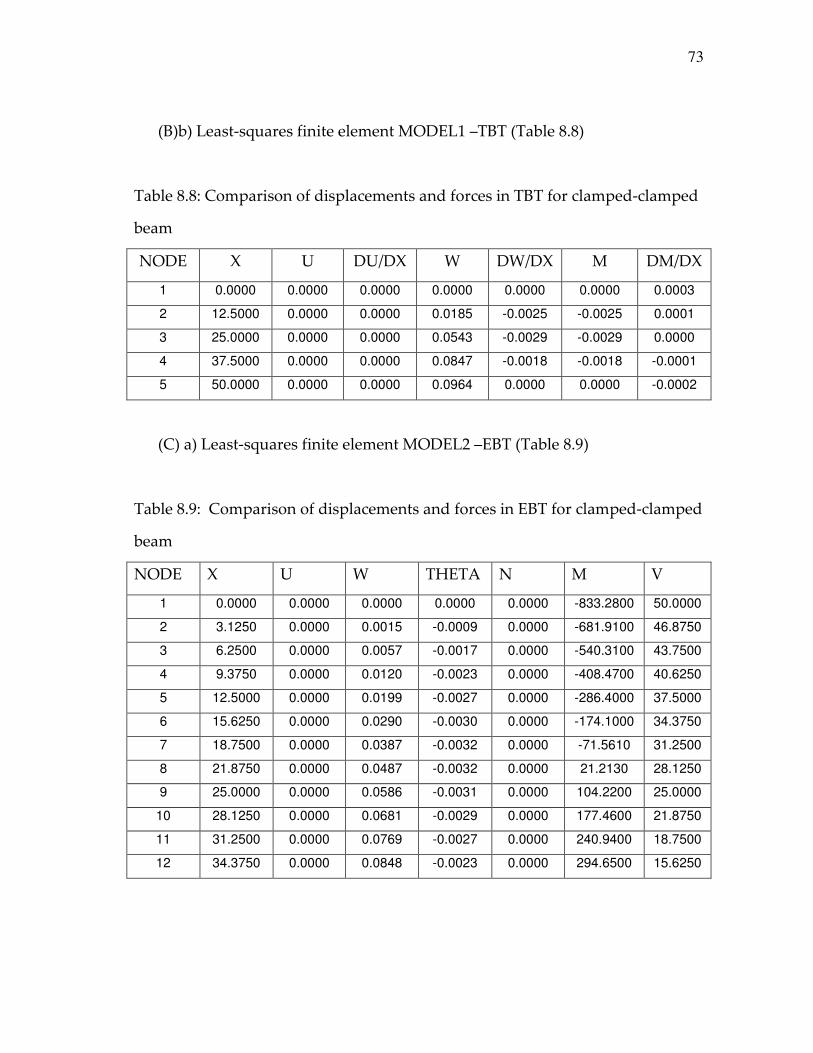
73

(B)b) Least-squares finite element MODEL1 –TBT (Table 8.8)

Table 8.8: Comparison of displacements and forces in TBT for clamped-clamped

beam


1 0.0000 0.0000 0.0000 0.0000 0.0000 0.0000 0.0003

2 12.5000 0.0000 0.0000 0.0185 -0.0025 -0.0025 0.0001

3 25.0000 0.0000 0.0000 0.0543 -0.0029 -0.0029 0.0000

4 37.5000 0.0000 0.0000 0.0847 -0.0018 -0.0018 -0.0001

5 50.0000 0.0000 0.0000 0.0964 0.0000 0.0000 -0.0002

(C) a) Least-squares finite element MODEL2 –EBT (Table 8.9)

Table 8.9: Comparison of displacements and forces in EBT for clamped-clamped

beam


1 0.0000 0.0000 0.0000 0.0000 0.0000 -833.2800 50.0000

2 3.1250 0.0000 0.0015 -0.0009 0.0000 -681.9100 46.8750

3 6.2500 0.0000 0.0057 -0.0017 0.0000 -540.3100 43.7500

4 9.3750 0.0000 0.0120 -0.0023 0.0000 -408.4700 40.6250

5 12.5000 0.0000 0.0199 -0.0027 0.0000 -286.4000 37.5000

6 15.6250 0.0000 0.0290 -0.0030 0.0000 -174.1000 34.3750

7 18.7500 0.0000 0.0387 -0.0032 0.0000 -71.5610 31.2500

8 21.8750 0.0000 0.0487 -0.0032 0.0000 21.2130 28.1250

9 25.0000 0.0000 0.0586 -0.0031 0.0000 104.2200 25.0000

10 28.1250 0.0000 0.0681 -0.0029 0.0000 177.4600 21.8750

11 31.2500 0.0000 0.0769 -0.0027 0.0000 240.9400 18.7500

12 34.3750 0.0000 0.0848 -0.0023 0.0000 294.6500 15.6250

74



13 37.5000 0.0000 0.0916 -0.0020 0.0000 338.6000 12.5000

14 40.6250 0.0000 0.0970 -0.0015 0.0000 372.7800 9.3750

15 43.7500 0.0000 0.1009 -0.0010 0.0000 397.1900 6.2500

16 46.8750 0.0000 0.1034 -0.0005 0.0000 411.8400 3.1250

17 50.0000 0.0000 0.1042 0.0000 0.0000 416.7200 0.0000


Table 8.10: Comparison of displacements and forces in TBT for clamped-

clamped beam

NODE X U W φ N M V

1 0.0000 0.0000 0.0000 0.0000 0.0000 -833.1500 49.9960

2 3.1250 0.0000 0.0015 -0.0009 0.0000 -681.7900 46.8710

3 6.2500 0.0000 0.0057 -0.0017 0.0000 -540.2000 43.7460

4 9.3750 0.0000 0.0120 -0.0023 0.0000 -408.3800 40.6210

5 12.5000 0.0000 0.0199 -0.0027 0.0000 -286.3200 37.4960

6 15.6250 0.0000 0.0289 -0.0030 0.0000 -174.0300 34.3710

7 18.7500 0.0000 0.0386 -0.0032 0.0000 -71.5020 31.2470

8 21.8750 0.0000 0.0486 -0.0032 0.0000 21.2620 28.1220

9 25.0000 0.0000 0.0585 -0.0031 0.0000 104.2600 24.9970

10 28.1250 0.0000 0.0680 -0.0029 0.0000 177.4900 21.8720

11 31.2500 0.0000 0.0768 -0.0027 0.0000 240.9600 18.7480

12 34.3750 0.0000 0.0847 -0.0023 0.0000 294.6700 15.6230

13 37.5000 0.0000 0.0914 -0.0020 0.0000 338.6100 12.4980

14 40.6250 0.0000 0.0968 -0.0015 0.0000 372.7800 9.3738

15 43.7500 0.0000 0.1008 -0.0010 0.0000 397.1900 6.2492

16 46.8750 0.0000 0.1032 -0.0005 0.0000 411.8400 3.1246

17 50.0000 0.0000 0.1040 0.0000 0.0000 416.7200 0.0000

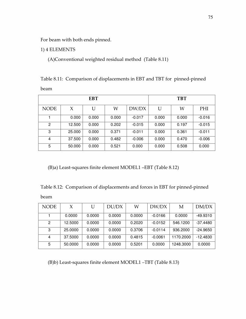
75

For beam with both ends pinned.

1) 4 ELEMENTS

(A)Conventional weighted residual method (Table 8.11)

Table 8.11: Comparison of displacements in EBT and TBT for pinned-pinned

beam

EBT TBT


1 0.000 0.000 0.000 -0.017 0.000 0.000 -0.016

2 12.500 0.000 0.202 -0.015 0.000 0.197 -0.015

3 25.000 0.000 0.371 -0.011 0.000 0.361 -0.011

4 37.500 0.000 0.482 -0.006 0.000 0.470 -0.006

5 50.000 0.000 0.521 0.000 0.000 0.508 0.000

(B)a) Least-squares finite element MODEL1 –EBT (Table 8.12)

Table 8.12: Comparison of displacements and forces in EBT for pinned-pinned

beam


1 0.0000 0.0000 0.0000 0.0000 -0.0166 0.0000 -49.9310

2 12.5000 0.0000 0.0000 0.2020 -0.0152 546.1200 -37.4480

3 25.0000 0.0000 0.0000 0.3706 -0.0114 936.2000 -24.9650

4 37.5000 0.0000 0.0000 0.4815 -0.0061 1170.2000 -12.4830

5 50.0000 0.0000 0.0000 0.5201 0.0000 1248.3000 0.0000

(B)b) Least-squares finite element MODEL1 –TBT (Table 8.13)

76

Table 8.13: Comparison of displacements and forces in TBT for pinned-pinned

beam


1 0.0000 0.0000 0.0000 0.0000 -0.0152 -0.0152 0.0000

2 12.5000 0.0000 0.0000 0.1844 -0.0139 -0.0139 -0.0002

3 25.0000 0.0000 0.0000 0.3386 -0.0105 -0.0105 -0.0003

4 37.5000 0.0000 0.0000 0.4402 -0.0056 -0.0056 -0.0004

5 50.0000 0.0000 0.0000 0.4756 0.0000 0.0000 -0.0005

(C)a) Least-squares finite element MODEL2 –EBT (Table 8.14)

Table 8.14: Comparison of displacements and forces in EBT for pinned-pinned

beam


1 0.0000 0.0000 0.0000 -0.0167 0.0000 0.0000 50.0000

2 3.1250 0.0000 0.0520 -0.0166 0.0000 151.3700 46.8750

3 6.2500 0.0000 0.1034 -0.0163 0.0000 292.9700 43.7500

4 9.3750 0.0000 0.1536 -0.0158 0.0000 424.8000 40.6250

5 12.5000 0.0000 0.2022 -0.0152 0.0000 546.8800 37.5000

6 15.6250 0.0000 0.2487 -0.0145 0.0000 659.1800 34.3750

7 18.7500 0.0000 0.2926 -0.0136 0.0000 761.7200 31.2500

8 21.8750 0.0000 0.3335 -0.0126 0.0000 854.4900 28.1250

9 25.0000 0.0000 0.3711 -0.0115 0.0000 937.5000 25.0000

10 28.1250 0.0000 0.4050 -0.0102 0.0000 1010.7000 21.8750

77



11 31.2500 0.0000 0.4350 -0.0089 0.0000 1074.2000 18.7500

12 34.3750 0.0000 0.4608 -0.0076 0.0000 1127.9000 15.6250

13 37.5000 0.0000 0.4822 -0.0061 0.0000 1171.9000 12.5000

14 40.6250 0.0000 0.4990 -0.0046 0.0000 1206.1000 9.3750

15 43.7500 0.0000 0.5111 -0.0031 0.0000 1230.5000 6.2500

16 46.8750 0.0000 0.5184 -0.0016 0.0000 1245.1000 3.1250

17 50.0000 0.0000 0.5208 0.0000 0.0000 1250.0000 0.0000


Table 8.15: Comparison of displacements and forces in TBT for pinned-pinned

beam

NODE X U W φ N M ddx

φ

1 0.0000 0.0000 0.0000 -0.0167 0.0000 0.0000 49.9960

2 3.1250 0.0000 0.0520 -0.0166 0.0000 151.3500 46.8710

3 6.2500 0.0000 0.1033 -0.0163 0.0000 292.9400 43.7460

4 9.3750 0.0000 0.1536 -0.0158 0.0000 424.7700 40.6210

5 12.5000 0.0000 0.2022 -0.0152 0.0000 546.8200 37.4960

6 15.6250 0.0000 0.2486 -0.0145 0.0000 659.1200 34.3710

7 18.7500 0.0000 0.2925 -0.0136 0.0000 761.6500 31.2470

8 21.8750 0.0000 0.3334 -0.0126 0.0000 854.4100 28.1220

9 25.0000 0.0000 0.3710 -0.0115 0.0000 937.4100 24.9970

10 28.1250 0.0000 0.4049 -0.0102 0.0000 1010.6000 21.8720

11 31.2500 0.0000 0.4349 -0.0089 0.0000 1074.1000 18.7480

12 34.3750 0.0000 0.4606 -0.0076 0.0000 1127.8000 15.6230

78


NODE X U W φ N M ddx

φ

13 37.5000 0.0000 0.4820 -0.0061 0.0000 1171.8000 12.4980

14 40.6250 0.0000 0.4988 -0.0046 0.0000 1205.9000 9.3738

15 43.7500 0.0000 0.5109 -0.0031 0.0000 1230.3000 6.2492

16 46.8750 0.0000 0.5182 -0.0016 0.0000 1245.0000 3.1246

17 50.0000 0.0000 0.5207 0.0000 0.0000 1249.9000 0.0000

A comparison of finite element results for deflection of beams with pinned-

pinned boundary conditions under uniformly distributed load for EBT is shown

below in Table 8.16.

Table 8.16: A comparison of results for deflection of beams with pinned-pinned

boundary conditions under uniformly distributed load for EBT

q 4 elements 8 elements 32 elements

1 0.30146 0.30146 0.30146

2 0.54802 0.54802 0.54802

3 0.73099 0.73099 0.73099

4 0.86628 0.86628 0.86628

5 0.96642 0.96642 0.96642

6 1.03840 1.03840 1.03840

7 1.08530 1.08530 1.08530

8 1.10720 1.10720 1.10720

79



9 1.10090 1.10090 1.10090

10 1.05980 1.05980 1.05980

A comparison of finite element results for deflection of beams with pinned-

pinned boundary conditions under uniformly distributed load for TBT is shown

below in Table 8.17 .

Table 8.17: A comparison of results for deflection of beams with pinned-pinned

boundary conditions under uniformly distributed load for TBT


1 0.30134 0.30134 0.30134

2 0.54781 0.54781 0.54781

3 0.73069 0.73069 0.73069

4 0.86590 0.86590 0.86590

5 0.96597 0.96597 0.96597

6 1.03790 1.03790 1.03790

7 1.08470 1.08470 1.08470

8 1.10650 1.10650 1.10650

9 1.10020 1.10020 1.10020

10 1.05900 1.05900 1.05900

80

A comparison of finite element results for deflection of beams with hinged-

hinged boundary conditions under uniformly distributed load for EBT is shown


Table 8.18: A comparison of results for deflection of beams with hinged-hinged

boundary conditions under uniformly distributed load for EBT


1 0.52083 0.52083 0.52083

2 1.04170 1.04170 1.04170

3 1.56250 1.56250 1.56250

4 2.08330 2.08330 2.08330

5 2.60420 2.60420 2.60420

6 3.12500 3.12500 3.12500

7 3.64580 3.64580 3.64580

8 4.16670 4.16670 4.16670

9 4.68750 4.68750 4.68750

10 5.20830 5.20830 5.20830

A comparison of finite element results for deflection of beams with hinged-

hinged boundary conditions under uniformly distributed load for TBT is shown


81

Table 8.19: A comparison of results for deflection of beams with hinged-hinged

boundary conditions under uniformly distributed load for TBT


1 0.52096 0.52096 0.52096

2 1.04190 1.04190 1.04190

3 1.56290 1.56290 1.56290

4 2.08380 2.08380 2.08380

5 2.60480 2.60480 2.60480

6 3.12570 3.12580 3.12570

7 3.64670 3.64670 3.64670

8 4.16770 4.16770 4.16770

9 4.68860 4.68860 4.68860

10 5.20960 5.20960 5.20960

A comparison of finite element results for deflection of beams with clamped-

clamped boundary conditions under uniformly distributed load for EBT is

shown below in Table 8.20.

Table 8.20: A comparison of results for deflection of beams with clamped-

clamped boundary conditions under uniformly distributed load for EBT


1 0.10410 0.10410 0.10410

2 0.20778 0.20778 0.20778

3 0.31065 0.31065 0.31067

82



4 0.41234 0.41234 0.41234

5 0.51250 0.51250 0.51259

6 0.61086 0.61086 0.61104

7 0.70718 0.70718 0.70750

8 0.80128 0.80128 0.80180

9 0.89305 0.89305 0.89390

10 0.98239 0.98239 0.98349

A comparison of finite element results for deflection of beams with clamped-

clamped boundary conditions under uniformly distributed load for TBT is

shown below in Table 8.21.

Table 8.21: A comparison of results for deflection of beams with clamped-

clamped boundary conditions under uniformly distributed load for TBT


1 0.10422 0.10422 0.10422

2 0.20803 0.20803 0.20803

3 0.31102 0.31102 0.31103

4 0.41282 0.41282 0.41286

5 0.51310 0.51320 0.51319

6 0.61157 0.61157 0.61175

7 0.70799 0.70799 0.70831

83



8 0.80219 0.80219 0.80271

9 0.89405 0.89405 0.89483

10 0.98348 0.98348 0.98458

8.3. Plots

The plot of x vs deflection (w) for different formulations and different

elements is shown below in Figures 8.1 and 8.2.

The following are the plots for comparison of a beam clamped at both ends and

divided in 4 equal elements.

EBT- 4 elements

0.0000

0.0200

0.0400

0.0600

0.0800

0.1000

0.1200

0.00 10.00 20.00 30.00 40.00 50.00 60.00x

de

fle

cti

on

w

x vs LSFEM MODEL1

x vs conventional method

x vs LSFEM MODEL2

x vs exact solution

Figure 8.1. Comparison of x vs. deflection in different models for EBT,

clamped-clamped, 4 elements

84

TBT- 4 elements

0.0000

0.0200

0.0400

0.0600

0.0800

0.1000

0.1200

0.00 10.00 20.00 30.00 40.00 50.00 60.00x

de

fle

cti

on

w

x vsLSFEM MODEL1


x vs LSFEM MODEL2

x vs exact solution

Figure 8.2. Comparison of x vs. deflection in different models for TBT, clamped-

clamped ,4 elements


divided in 8 equal elements in Figures 8.3 and 8.4.

85

EBT -8 elements

0.0000

0.0200

0.0400

0.0600

0.0800

0.1000

0.1200

0.00 10.00 20.00 30.00 40.00 50.00 60.00x

de

fle

cti

on

w

x vs LSFEM MODEL1

x vs conventionall method

x vs LSFEM MODEL2

x vs exact solution

Figure 8.3. Comparison of x vs. deflection in different models for EBT, clamped-

clamped, 8 elements

0.0000

0.0200

0.0400

0.0600

0.0800

0.1000

0.1200

0.00 10.00 20.00 30.00 40.00 50.00 60.00

de

fle

cti

on

w

x

TBT-8 elements

x vsLSFEM MODEL1


x vs LSFEM MODEL2

x vs exact solution

Figure 8.4. Comparison of x vs. deflection in different models for

TBT, clamped-clamped, 8 elements

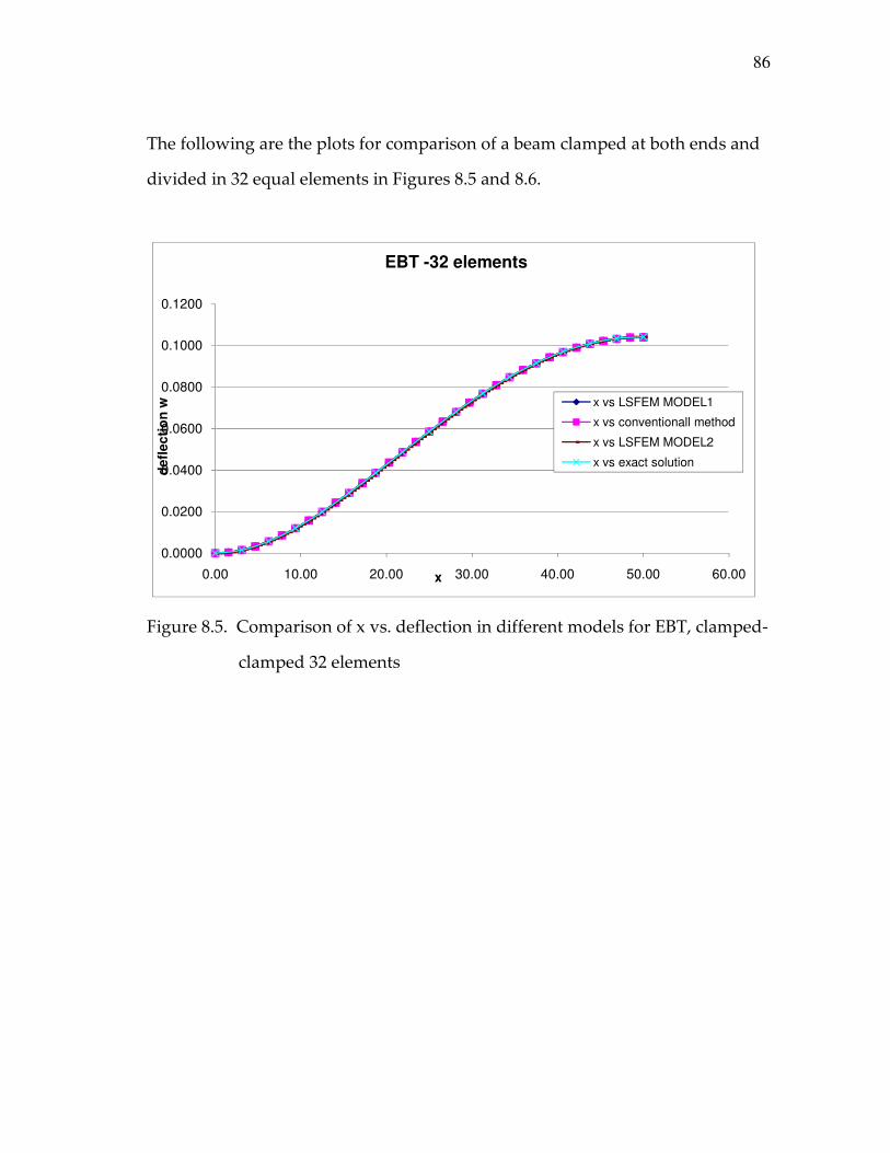
86


divided in 32 equal elements in Figures 8.5 and 8.6.

0.0000

0.0200

0.0400

0.0600

0.0800

0.1000

0.1200

0.00 10.00 20.00 30.00 40.00 50.00 60.00

de

fle

cti

on

w

x

EBT -32 elements

x vs LSFEM MODEL1


x vs LSFEM MODEL2

x vs exact solution

Figure 8.5. Comparison of x vs. deflection in different models for EBT, clamped-

clamped 32 elements

87

0.0000

0.0200

0.0400

0.0600

0.0800

0.1000

0.1200

0.00 10.00 20.00 30.00 40.00 50.00 60.00

defl

ecti

on

w

x

TBT -32 elements

x vs LSFEM MODEL1


x vs LSFEM MODEL2

x vs exact solution

Figure 8.6. Comparison of x vs. deflection in different models for TBT, clamped-

clamped 32 elements

The following are the plots for comparison of a beam hinged at both ends and

divided in 4 equal elements in Figures 8.7and 8.8.

88

EBT - 4 elements

0.0000

0.0500

0.1000

0.1500

0.2000

0.2500

0.3000

0.3500

0.4000

0.4500

0.5000

0.5500

0.0000 10.0000 20.0000 30.0000 40.0000 50.0000 60.0000x

defl

ecti

on

w x vs LSFEM MODEL1


x vs LSFEM MODEL2

x vs exact solution

Figure 8.7. Comparison of x vs. deflection in different models for EBT, hinged-

hinged ,4 elements

89

0.0000

0.0500

0.1000

0.1500

0.2000

0.2500

0.3000

0.3500

0.4000

0.4500

0.5000

0.5500

0.0000 10.0000 20.0000 30.0000 40.0000 50.0000 60.0000

defl

ecti

on

w

x

TBT - 4 elements

x vs LSFEM MODEL1


x vs LSFEM MODEL2

x vs exact solution

Figure 8.8. Comparison of x vs. deflection in different models for TBT, hinged-

hinged, 4 elements



90

0.0000

0.0500

0.1000

0.1500

0.2000

0.2500

0.3000

0.3500

0.4000

0.4500

0.5000

0.5500

0.00 10.00 20.00 30.00 40.00 50.00 60.00

defl

ecti

on

w

x

EBT -8 elements

x vs LSFEM MODEL1


x vs LSFEM MODEL2

x vs exact solution

Figure 8.9. Comparison of x vs. deflection in different models for EBT, hinged-

hinged,8 elements

TBT-8 elements

0.0000

0.0500

0.1000

0.1500

0.2000

0.2500

0.3000

0.3500

0.4000

0.4500

0.5000

0.5500

0.00 10.00 20.00 30.00 40.00 50.00 60.00x

de

fle

cti

on

w x vsLSFEM MODEL1


x vs LSFEM MODEL2

x vs exact solution

Figure 8.10. Comparison of x vs. deflection in different models for TBT,

hinged-hinged,8 elements

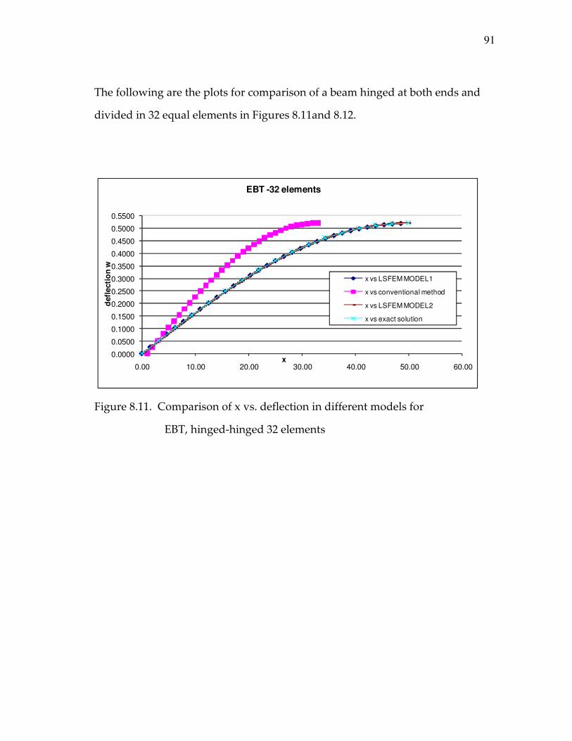
91



0.0000

0.0500

0.1000

0.1500

0.2000

0.2500

0.3000

0.3500

0.4000

0.4500

0.5000

0.5500

0.00 10.00 20.00 30.00 40.00 50.00 60.00

defl

ecti

on

w

x

EBT -32 elements

x vs LSFEM MODEL1


x vs LSFEM MODEL2

x vs exact solution


EBT, hinged-hinged 32 elements

92

TBT -32 elements

0.0000

0.0500

0.1000

0.1500

0.2000

0.2500

0.3000

0.3500

0.4000

0.4500

0.5000

0.5500

0.00 10.00 20.00 30.00 40.00 50.00 60.00x

defl

ecti

on

w x vs LSFEM MODEL1


x vs LSFEM MODEL2

x vs exact solution


TBT, hinged-hinged 32 elements

The following are the plots for comparison of a beam pinned at both ends and


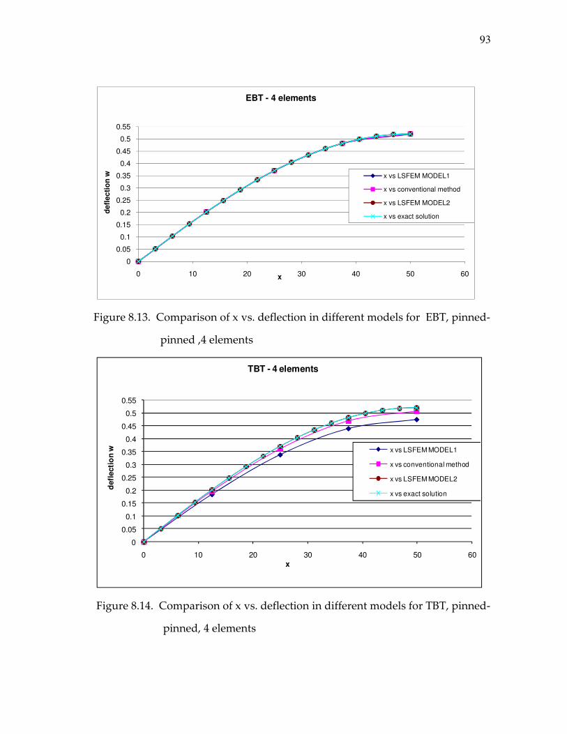
93

0

0.05

0.1

0.15

0.2

0.25

0.3

0.35

0.4

0.45

0.5

0.55

0 10 20 30 40 50 60

defl

ecti

on

w

x

EBT - 4 elements

x vs LSFEM MODEL1


x vs LSFEM MODEL2

x vs exact solution

Figure 8.13. Comparison of x vs. deflection in different models for EBT, pinned-

pinned ,4 elements

0

0.05

0.1

0.15

0.2

0.25

0.3

0.35

0.4

0.45

0.5

0.55

0 10 20 30 40 50 60

defl

ecti

on

w

x

TBT - 4 elements

x vs LSFEM MODEL1


x vs LSFEM MODEL2

x vs exact solution

Figure 8.14. Comparison of x vs. deflection in different models for TBT, pinned-

pinned, 4 elements

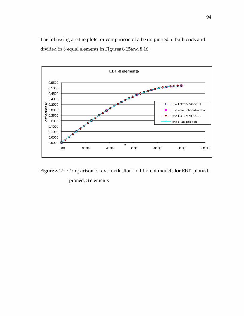
94



0.0000

0.0500

0.1000

0.1500

0.2000

0.2500

0.3000

0.3500

0.4000

0.4500

0.5000

0.5500

0.00 10.00 20.00 30.00 40.00 50.00 60.00

defl

ecti

on

w

x

EBT -8 elements

x vs LSFEM MODEL1


x vs LSFEM MODEL2

x vs exact solution


pinned, 8 elements

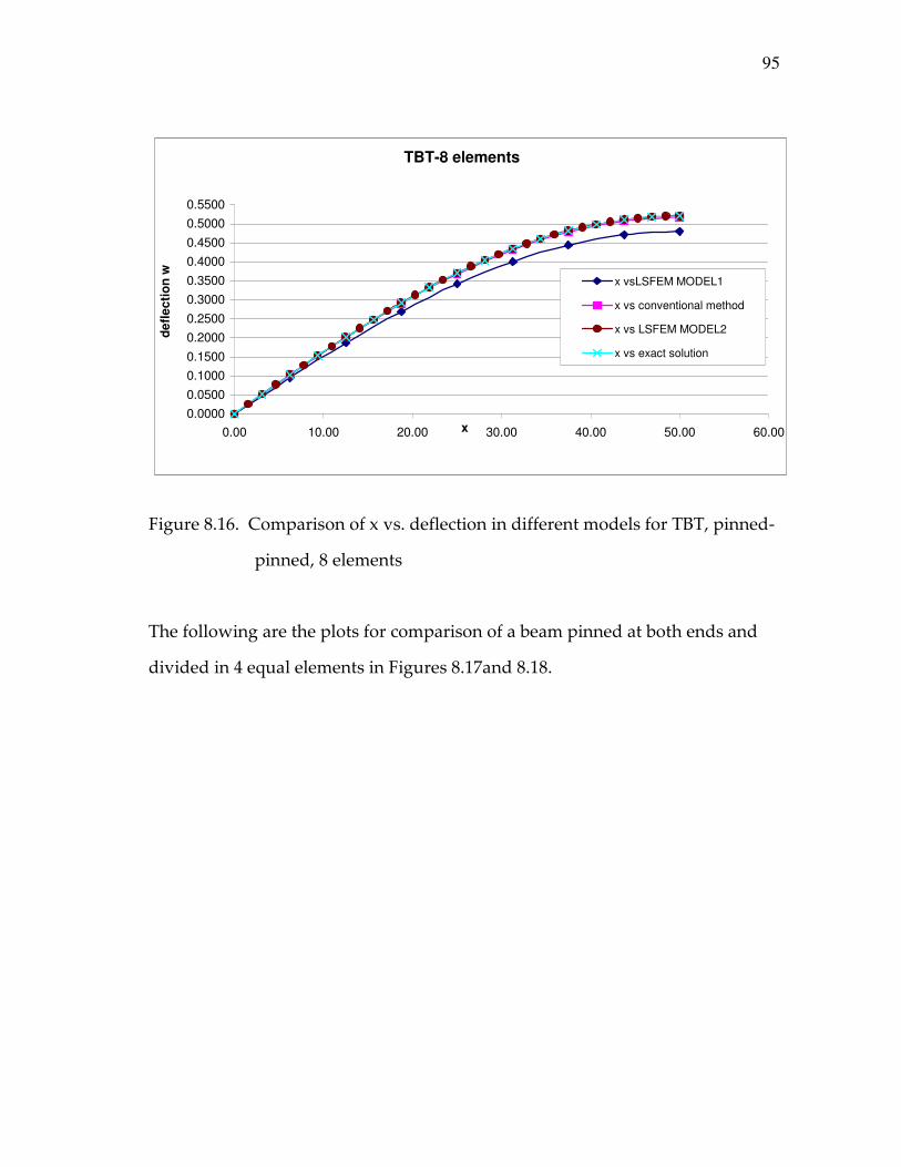
95

TBT-8 elements

0.0000

0.0500

0.1000

0.1500

0.2000

0.2500

0.3000

0.3500

0.4000

0.4500

0.5000

0.5500

0.00 10.00 20.00 30.00 40.00 50.00 60.00x

de

fle

cti

on

w

x vsLSFEM MODEL1


x vs LSFEM MODEL2

x vs exact solution


pinned, 8 elements



96

EBT -32 elements

0.0000

0.0500

0.1000

0.1500

0.2000

0.2500

0.3000

0.3500

0.4000

0.4500

0.5000

0.5500

0.00 10.00 20.00 30.00 40.00 50.00 60.00x

defl

ecti

on

w

x vs LSFEM MODEL1


x vs LSFEM MODEL2

x vs exact solution


pinned, 32 elements

0.0000

0.0500

0.1000

0.1500

0.2000

0.2500

0.3000

0.3500

0.4000

0.4500

0.5000

0.5500

0.00 10.00 20.00 30.00 40.00 50.00 60.00

defl

ecti

on

w

x

TBT -32 elements

x vs LSFEM MODEL1


x vs LSFEM MODEL2

x vs exact solution


pinned 32 elements

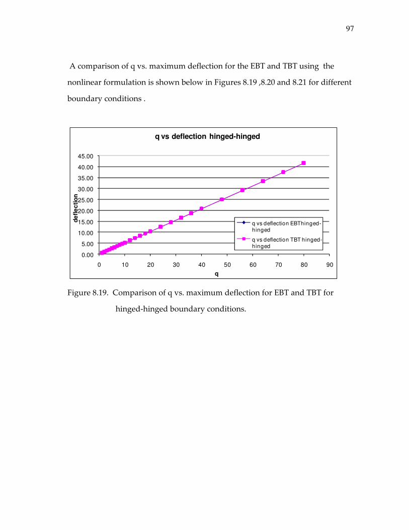
97

A comparison of q vs. maximum deflection for the EBT and TBT using the

nonlinear formulation is shown below in Figures 8.19 ,8.20 and 8.21 for different

boundary conditions .

0.00

5.00

10.00

15.00

20.00

25.00

30.00

35.00

40.00

45.00

0 10 20 30 40 50 60 70 80 90

de

fle

cti

on

q

q vs deflection hinged-hinged

q vs deflection EBThinged-hinged

q vs deflection TBT hinged-hinged

Figure 8.19. Comparison of q vs. maximum deflection for EBT and TBT for

hinged-hinged boundary conditions.

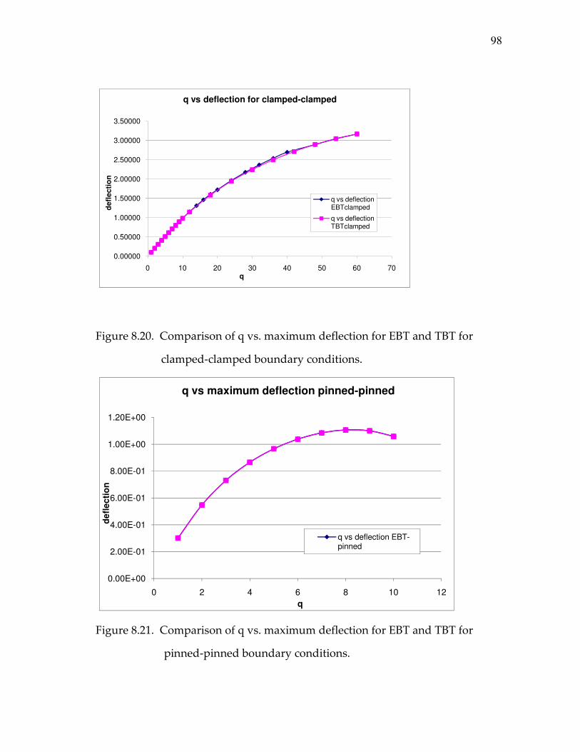
98

0.00000

0.50000

1.00000

1.50000

2.00000

2.50000

3.00000

3.50000

0 10 20 30 40 50 60 70

defl

ecti

on

q

q vs deflection for clamped-clamped

q vs deflection EBTclamped

q vs deflection TBTclamped


clamped-clamped boundary conditions.

0.00E+00

2.00E-01

4.00E-01

6.00E-01

8.00E-01

1.00E+00

1.20E+00

0 2 4 6 8 10 12

de

fle

cti

on

q

q vs maximum deflection pinned-pinned

q vs deflection EBT-pinned


pinned-pinned boundary conditions.

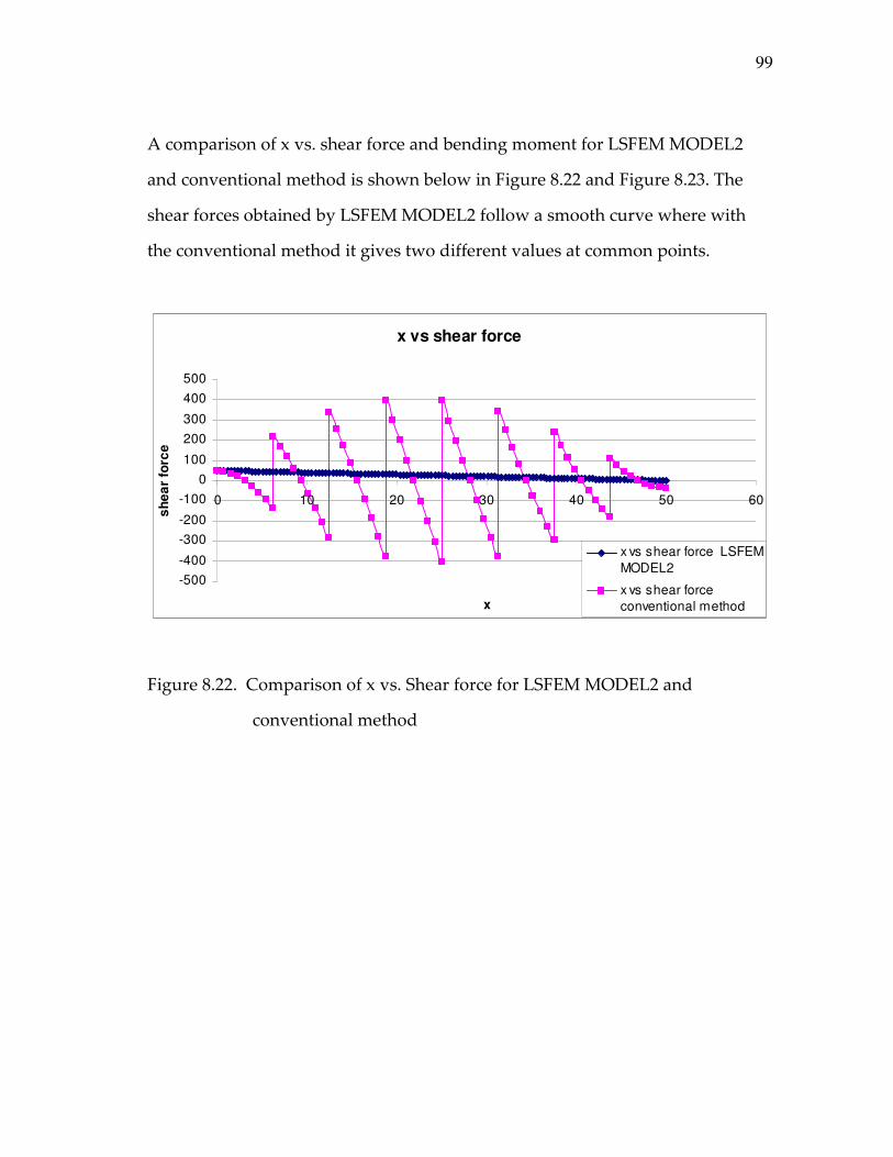
99

A comparison of x vs. shear force and bending moment for LSFEM MODEL2

and conventional method is shown below in Figure 8.22 and Figure 8.23. The

shear forces obtained by LSFEM MODEL2 follow a smooth curve where with

the conventional method it gives two different values at common points.

x vs shear force

-500

-400

-300

-200

-100

0

100

200

300

400

500

0 10 20 30 40 50 60

x

sh

ea

r fo

rce

x vs shear force LSFEM

MODEL2

x vs shear force

conventional method

Figure 8.22. Comparison of x vs. Shear force for LSFEM MODEL2 and

conventional method

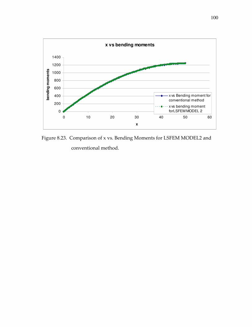
100

x vs bending moments

0

200

400

600

800

1000

1200

1400

0 10 20 30 40 50 60

x

be

nd

ing

mo

me

nts

x vs Bending moment for

conventional method

x vs bending moment

forLSFEM MODEL 2

Figure 8.23. Comparison of x vs. Bending Moments for LSFEM MODEL2 and

conventional method.

101

9. SUMMARY AND CONCLUSIONS

From the results presented in section 8, the following observations and

conclusions can be made:

1) The plots of x vs. deflection for LSFEM MODEL 1, LSFEM MODEL 2, and

conventional method closely fit the exact solution curve. A good solution

accuracy for deflection of LSFEM MODEL2 can be observed even for

lesser number of elements for various boundary conditions.

2) As the number of elements increases, the plots of x vs. deflection for

LSFEM MODEL 1, LSFEM MODEL 2, and conventional method coincide

with the exact solution curve for different boundary conditions.

3) The least-squares method helps introducing forces and moments as

primary variables and helps increasing the accuracy of the solution.

4) Another salient feature of least-squares method is that once the boundary

conditions are imposed the discretization always leads to a positive-

definite system of equations which allow the use of fast iterative methods

for solution.

5) Thus the theoretical and computational advantages of using the least-

squares finite element model were discussed and verified using

numerical examples with different boundary conditions and number of

elements.

6) Since the internal forces and bending moments serve as independent

variables, they can be obtained simultaneously unlike the conventional

weighted residual method.

102

9.1 Future Work

Based on the present study, a systematic and fair comparison of weak

form Galerkin models with least-squares models for problems involving plates

and shells as well as fluid dynamics can be done further.

103

REFERENCES

[1] J.P. Pontaza, Least-squares variational principles and the finite element

method: theory, formulations, and models for solid and fluid mechanics,

Finite Elements in Analysis and Design 41 (2005) 703–728.

[2] F. Moleiro, C.M. Mota Soares, C.A. Mota Soares, J.N. Reddy, Mixed

least-squares finite element model for the static analysis of laminated

composite plates, Computers and Structures 86 (2008) 826–838.

[3] J.N. Reddy, An Introduction to Nonlinear Finite Element Analysis,

Oxford University Press Inc., Oxford, 2004.

[4] J.N. Reddy, An Introduction to the Finite Element Method, 3rd ed.,

McGraw-Hill, New York, 2006.

[5] Kikuchi F., Aizawa T., Locking phenomena in finite element analysis of

large deflection problems. Proc. 32nd Japan Congress of Applied

Mechanics, University of Tokyo Press, Tokyo, 1982.

[6] R. Murali and G. Prathap, Field-consistency Aspects in Geometrically

Non-linear Beam Formulation, CSIR Center for Mathematical Modeling

and Computer Simulation, July 2006.

[7] L. G. Selna, M.A. Hakam, Least square methods in structural analysis,

Computers and Structures 80 (2002) 2011-2025, July 2002.

[8] Z. Wieckowski, M. Golubiewski, Improvement in accuracy of finite

element method in analysis of stability of Euler-Bernoulli and

Timoshenko beams, Thin-Walled Structures 45 (2007) 950-954, September

2007.

104

[9] Suh-Yuh Yang, Jinn-Liang Liu, Analysis of least-squares finite element

methods for a parameter-dependent first-order system, Numer. Funct.

Anal. and Optimization, Numer. Funct. Analy. and Optimiz., 19(No.

1&2), (1998) 191-213.

[10] P. Fadum, K.S. Surana, A least-squares finite element formulation for

plane elasto-statics based on p-version with applications to laminated

composites, Computers and Structures 53. No. 3, (1994) 491-507.

[11] O.C. Zienkiewicz and D. R. J. Owen, Least squares finite element for

elasto-static problems. Int. J. Numer. Meth. Eng. 8, (1974) 341-358.

[12] Karl Grosh, Peter. M. Pinsky, Galerkin generalized least squares finite

element methods for time-harmonic structural harmonics, Comp. Meth.

in Appl. Mech. And Engg 154 (1998) 299-318.

[13] J. P. Pontaza, J. N. Reddy, Least-squares finite element formulation for

shear-deformable shells, Comp. Meth. In Appl. Mech. And Engg. 194

(2005) 2464-2493.

[14] J. P. Pontaza and J. N. Reddy, Spectral/hp least-squares finite element

formulation for the Navier-Stokes equations, Jour. Comp. Phys.,

190(2003), 523-549.

[15] V. Prabhakar and J. N. Reddy, Spectral/hp penalty least-squares finite

element formulation for the steady incompressible Navier-Stokes

equations, Jour. Comp. Phys., 215 (2006), 274-297.

105

APPENDIX A

COMMON BEAM FORMULAE (http://structsource.com/analysis/types/beam.htm)

106

VITA

Ameeta Amar Raut was born in Pune, India. She received her Bachelor of

Engineering degree (with distinction) in the field of mechanical engineering

from Government College of Engineering, Pune, India in August 2006. She

entered the mechanical engineering program at Texas A&M University, College

Station, TX in Fall 2006 to pursue her Master of Science degree. Her research

interests include design & analysis of structures & materials for various

industrial applications.

Ms. Raut may be reached at: Texas A&M University, Department of

Mechanical Engineering, 3123 TAMU, College Station TX 77843-3123. Her email

is: [email protected].

nonlinear analysis of beams using least-squares finite...

Documents