nonparametric regression in r - faculty of social … regression in r ... nonparametric regression,...

Nonparametric Regression in R

An Appendix to An R Companion to Applied Regression, Second Edition

John Fox & Sanford Weisberg

last revision: 13 December 2010

Abstract

In traditional parametric regression models, the functional form of the model is specifiedbefore the model is fit to data, and the object is to estimate the parameters of the model. Innonparametric regression, in contrast, the object is to estimate the regression function directlywithout specifying its form explicitly. In this appendix to Fox and Weisberg (2011), we describehow to fit several kinds of nonparametric-regression models in R, including scatterplot smoothers,where there is a single predictor; models for multiple regression; additive regression models; andgeneralized nonparametric-regression models that are analogs to generalized linear models.

1 Nonparametric Regression Models

The traditional nonlinear regression model (described in the Appendix on nonlinear regression) fitsthe model

y = m(x,�) + "

where � is a vector of parameters to be estimated, and x is a vector of predictors; the errors "are assumed to be normally and independently distributed with mean 0 and constant variance �2.The function m(x,�), relating the average value of the response y to the predictors, is specified inadvance, as it is in a linear regression model.

The general nonparametric regression model is written in a similar manner, but the function mis left unspecified:

y = m(x) + "

= m(x1, x2, . . . , xp) + "

for the p predictors x = (x1, x2, . . . , xp)′. Moreover, the object of nonparametric regression is to

estimate the regression function m(x) directly, rather than to estimate parameters. Most methodsof nonparametric regression implicitly assume that m is a smooth, continuous function.1 As innonlinear regression, it is standard to assume that "i ∼ NID(0, �2).

An important special case of the general model is nonparametric simple regression, where thereis only one predictor:

y = m(x) + "

Nonparametric simple regression is often called “scatterplot smoothing” because an important ap-plication is to tracing a smooth curve through a scatterplot of y against x. We frequently usenonparametric regression in this manner in the body of the text.

1An exception to the implicit assumption of smoothness is wavelet regression, not discussed in this appendix,which is implemented in R, e.g., in the wavethresh package; see Nason and Silverman (1994, 2000); Nason (2008).

1

Because it is difficult to fit the general nonparametric regression model when there are manypredictors, and because it is difficult to display the fitted model when there are more than twoor three predictors, more restrictive models have been developed. One such model is the additiveregression model,

y = �0 +m1(x1) +m2(x2) + ⋅ ⋅ ⋅+mp(xp) + "

where the partial-regression functions mj(xj) are assumed to be smooth, and are to be estimatedfrom the data. This model is much more restrictive than the general nonparametric regressionmodel, but less restrictive than the linear regression model, which assumes that all of the partial-regression functions are linear.

Variations on the additive regression model include semiparametric models, in which some ofthe predictors enter linearly, for example,

y = �0 + �1x1 +m2(x2) + ⋅ ⋅ ⋅+mp(xp) + "

(particularly useful when some of the predictors are factors), and models in which some predictorsenter into interactions, which appear as higher-dimensional terms in the model, for example,

y = �0 +m12(x1, x2) +m3(x3) + ⋅ ⋅ ⋅+mp(xp) + "

All of these models extend straightforwardly to generalized nonparametric regression, much aslinear models extend to generalized linear models (discussed in Chapter 5 of the text). The randomand link components are as in generalized linear models, but the linear predictor of the GLM

� = �0 + �1x1 + �2x2 + ⋅ ⋅ ⋅+ �pxp

is replaced, for example, by an unspecified smooth function of the predictors

� = m(x1, x2, . . . , xp)

for the most general case, or by a sum of smooth partial-regression functions

� = �0 +m1(x1) +m2(x2) + ⋅ ⋅ ⋅+mp(xp)

in the generalized additive model.

2 Estimation

There are several approaches to estimating nonparametric regression models, of which we willdescribe two: local polynomial regression and smoothing splines. With respect to implementationof these methods in R, there is an embarrassment of riches:

� Local polynomial regression is performed by the standard R functions lowess (locally weightedscatterplot smoother, for the simple-regression case) and loess (local regression, more gen-erally).

� Simple-regression smoothing-spline estimation is performed by the standard R functionsmooth.spline.

� Generalized nonparametric regression by local likelihood estimation (of which local regressionis a special case for models with normal errors) is implemented in the locfit (local fitting)package (Loader, 1999), which also performs density estimation.

2

� Generalized additive models may be fit with Hastie and Tibshirani’s (1990) gam function(in the gam package), which uses spline or local-regression smoothers. The gam functionin Wood’s (2000, 2001, 2006) mgcv package, which is part of the standard R distribution,also fits this class of models using spline smoothers, and features automatic selection ofsmoothing parameters. (The name of the package comes from the method employed to pickthe smoothing parameters: multiple generalized cross-validation.)

� There are several other R package for nonparametric regression, including Bowman and Az-zalini’s (1997) sm (smoothing) package, which performs local-regression and local-likelihoodestimation, and which also includes facilities for nonparametric density estimation; and Gu’s(2000) gss (general smoothing splines) package, which fits various smoothing-spline regressionand generalized regression models. This is not an exhaustive list!

2.1 Local Polynomial Regression

2.1.1 Simple Regression

Here, we are looking to fit the modely = m(x) + "

Let us focus on evaluating the regression function at a particular x-value, x0. Ultimately, we will fitthe model at a representative range of values of x or simply at the n observations, xi. We proceedto perform a pth-order weighted-least-squares polynomial regression of y on x,

y = b0 + b1(x− x0) + b2(x− x0)2 + ⋅ ⋅ ⋅+ bp(x− x0)p + e

weighting the observations in relation to their proximity to the focal value x0; a common weightfunction to use is the tricube function:

W (z) =

{(1− ∣z∣3)3 for ∣z∣ < 1

0 for ∣z∣ ≥ 1

In the present context, z = (x − x0)/ℎ, where ℎ is the half-width of a window enclosing theobservations for the local regression. The fitted value at x0, that is, the estimated height of theregression curve, is simply y0 = b0, produced conveniently by having centered the predictor x atthe focal value x0.

It is typical to adjust ℎ so that each local regression includes a fixed proportion s of the data;then, s is called the span of the local-regression smoother. The larger the span, the smoother theresult; in contrast, the larger the order of the local regressions p, the more flexible the smooth, sothe span and the order of the local regressions can be traded off against one-another.

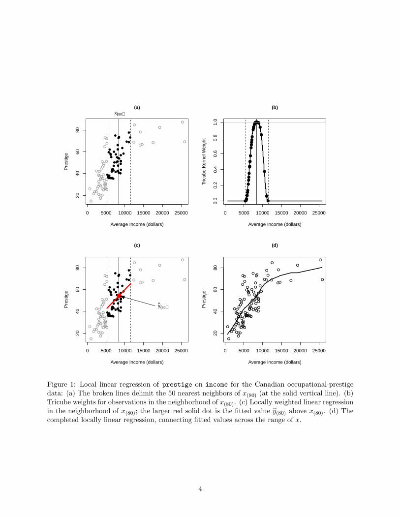
The process of fitting a local regression is illustrated in Figure 1, using the Canadian occupational-prestige data introduced in Chapter 2 of the text. We examine the regression of prestige onincome, focusing initially on the observation with the 80th largest income value, x(80), representedin Figure 1 by the vertical solid line.2

� A window including the 50 nearest x-neighbors of x(80) (i.e., for span s = 50/102 ≈ 1/2) isshown in Figure 1a.

� The tricube weights for observations in this neighborhood appear in Figure 1b.

2Cf., Figure 7.13 (page 345) in the text, for a similar figure explicating nearest-neighbor kernel regression.

3

0 5000 10000 15000 20000 25000

2040

6080

(a)

Average Income (dollars)

Pre

stig

e

●●●●

●

●●

●

●

●●

●

●

●●

●

●●

●

●

●

●

●

●

●

●

●

●

●

●

●

●

●

●

●

●

●

●

●

●

●

●●

●

●

●

●●

●

●

●

●

●●●

●

●●

●

●

●●

●

●

●

●

●

●

●

●

●

●

●

●

●

●

●

●

●●

●

●

●

●

●●

●

●

●

●

●

●

● ●

●

●

●

●●

●

●

●

x(80)

0 5000 10000 15000 20000 250000.

00.

20.

40.

60.

81.

0

(b)


Tric

ube

Ker

nel W

eigh

t●●●●●●●●●

●●●●

●●●●

●

●●●●●

●●●●●●●●●●●●●●●●●●●●●

●

●

●

●●

●

0 5000 10000 15000 20000 25000

2040

6080

(c)


Pre

stig

e

●●●●

●

●●

●

●

●●

●

●

●●

●

●●

●

●

●

●

●

●

●

●

●

●

●

●

●

●

●

●

●

●

●

●

●

●

●

●●

●

●

●

●●

●

●

●

●

●●●

●

●●

●

●

●●

●

●

●

●

●

●

●

●

●

●

●

●

●

●

●

●

●●

●

●

●

●

●●

●

●

●

●

●

●

● ●

●

●

●

●●

●

●

●

●

y(80)

●

●

●●●

●

●●

●

●

●●

●

●

●

●

●

●

●

●

●

●

●

●

●

●

●

●

●●

●

●

●

●

●●

●

●

●

●

●

●

●

●●●●

●

●●

●

●

●●

●

●

●●

●

●●

●

●

●

●

●

●

●

●

●

●

●

●

●

●

●

●

●

●

●

●

●

●

●

●●

●

●

●

●●

●

●

●

●

●

●

●●

●

●

●

0 5000 10000 15000 20000 25000

2040

6080

(d)


Pre

stig

e

Figure 1: Local linear regression of prestige on income for the Canadian occupational-prestigedata: (a) The broken lines delimit the 50 nearest neighbors of x(80) (at the solid vertical line). (b)Tricube weights for observations in the neighborhood of x(80). (c) Locally weighted linear regressionin the neighborhood of x(80); the larger red solid dot is the fitted value y(80) above x(80). (d) Thecompleted locally linear regression, connecting fitted values across the range of x.

4

� Figure 1c shows the locally weighted regression line fit to the data in the neighborhood of x0(i.e., a local polynomial regression of order p = 1); the fitted value y∣x(80) is represented inthis graph as a larger solid dot.

� Finally, in Figure 1d, local regressions are estimated for a range of x-values, and the fittedvalues are connected in a nonparametric-regression curve.

Figure 1d is produced by the following R commands, using the lowess function:

> library(car) # for data sets

> plot(prestige ˜ income, xlab="Average Income", ylab="Prestige", data=Prestige)

> with(Prestige, lines(lowess(income, prestige, f=0.5, iter=0), lwd=2))

The argument f to lowess gives the span of the local-regression smoother; iter=0 specifies thatthe local regressions should not be refit to down-weight outlying observations.3

2.1.2 Multiple Regression

The nonparametric multiple regression model is

y = f(x) + "

= f(x1, x2, . . . , xp) + "

Extending the local-polynomial approach to multiple regression is simple conceptually, but can runinto practical difficulties.

� The first step is to define a multivariate neighborhood around a focal point x′0 = (x01, x02, . . . , x0k).The default approach in the loess function is to employ scaled Euclidean distances:

D(xi,x0) =

√√√⎷ k∑j=1

(zij − z0j)2

where the zj are the standardized predictors,

zij =xij − xjsj

Here, xi is the predictor vector for the ith case; xij is the value of the jth predictor for theith case; xj is the mean of the jth predictor; and sj is its standard deviation.

� Weights are defined using the scaled distances:

wi = W

[D(xi,x0)

ℎ

]where W (⋅) is a suitable weight function, such as the tricube, in which case ℎ is the half-width(i.e., radius) of the neighborhood. As in local simple regression, ℎ may be adjusted to definea neighborhood including the [ns] nearest neighbors of x0 (where the square brackets denoterounding to the nearest integer).

3By default, lowess performs iter=3 robustness iterations, using a bisquare weight function. The idea of weightingobservations to obtain robust regression estimators is described in the Appendix on robust regression. Alternatively,one can use the loess.smooth function to get the coordinates for a local-polynomial smooth, or scatter.smooth todraw the graph.

5

� Perform a weighted polynomial regression of y on the x’s; for example, a local linear fit takesthe following form:

y = b0 + b1(x1 − x01) + b2(x2 − x02) + ⋅ ⋅ ⋅+ bk(xk − x0k) + e

The fitted value at x0 is then simply y0 = b0.

� The procedure is repeated for representative combinations of predictor values to build up apicture of the regression surface.

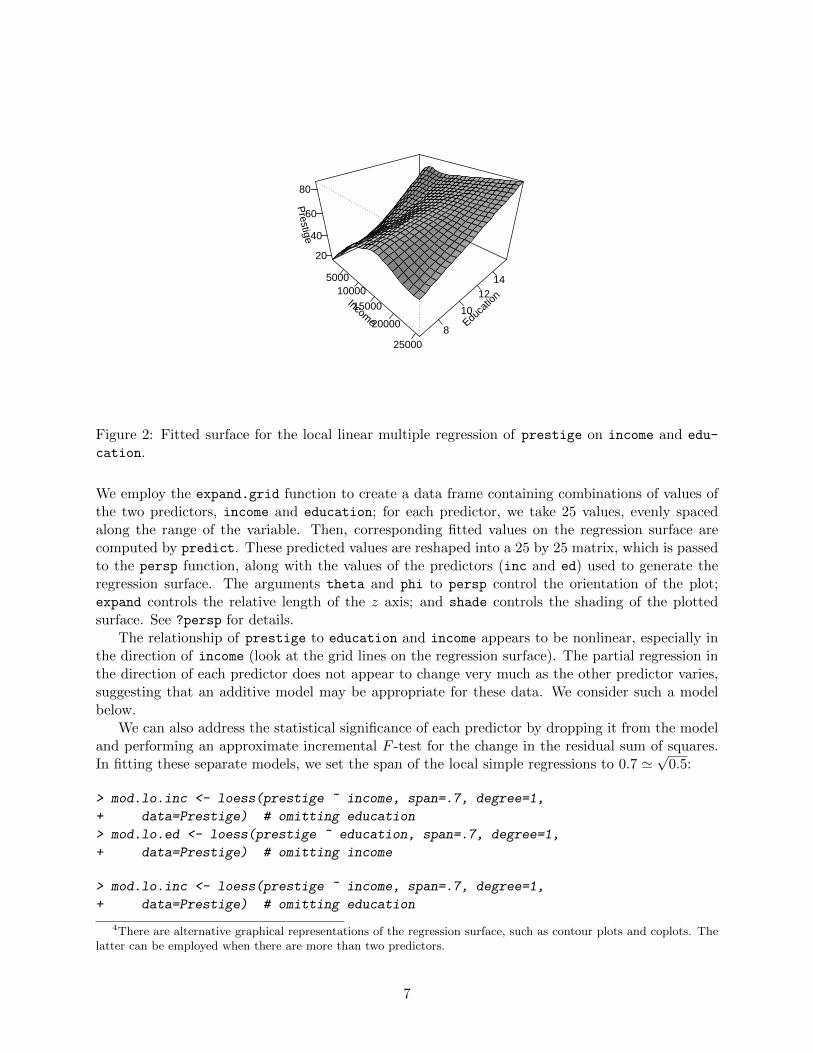
Extending the illustration of the previous section, and using the loess function, let us regressprestige on both the income and education levels of the occupations:

> mod.lo <- loess(prestige ˜ income + education, span=.5, degree=1, data=Prestige)

> summary(mod.lo)

Call:

loess(formula = prestige ˜ income + education, data = Prestige,

span = 0.5, degree = 1)

Number of Observations: 102

Equivalent Number of Parameters: 8.03

Residual Standard Error: 6.91

Trace of smoother matrix: 10.5

Control settings:

normalize: TRUE

span : 0.5

degree : 1

family : gaussian

surface : interpolate cell = 0.2

Specifying degree=1 fits locally linear regressions; the default is degree=2 (i.e., locally quadraticregressions). To see the full range of arguments for the loess function, consult ?loess. Thesummary output includes the standard deviation of the residuals under the model and an estimateof the equivalent number of parameters (or degrees of freedom) employed by the model — in thiscase, about eight parameters. In contrast, a standard linear regression model would have employedthree parameters (the constant and two slopes).

As in nonparametric simple regression, there are no parameters estimates: To see the result ofthe regression, we have to examine the fitted regression surface graphically, as in Figure 2, producedby the following R commands:4

> inc <- with(Prestige, seq(min(income), max(income), len=25))

> ed <- with(Prestige, seq(min(education), max(education), len=25))

> newdata <- expand.grid(income=inc, education=ed)

> fit.prestige <- matrix(predict(mod.lo, newdata), 25, 25)

> persp(inc, ed, fit.prestige, theta=45, phi=30, ticktype="detailed",

+ xlab="Income", ylab="Education", zlab="Prestige", expand=2/3,

+ shade=0.5)

6

Income

500010000

15000

20000

25000

Educa

tion

8

10

1214

Prestige

20

40

60

80

Figure 2: Fitted surface for the local linear multiple regression of prestige on income and edu-

cation.

We employ the expand.grid function to create a data frame containing combinations of values ofthe two predictors, income and education; for each predictor, we take 25 values, evenly spacedalong the range of the variable. Then, corresponding fitted values on the regression surface arecomputed by predict. These predicted values are reshaped into a 25 by 25 matrix, which is passedto the persp function, along with the values of the predictors (inc and ed) used to generate theregression surface. The arguments theta and phi to persp control the orientation of the plot;expand controls the relative length of the z axis; and shade controls the shading of the plottedsurface. See ?persp for details.

The relationship of prestige to education and income appears to be nonlinear, especially inthe direction of income (look at the grid lines on the regression surface). The partial regression inthe direction of each predictor does not appear to change very much as the other predictor varies,suggesting that an additive model may be appropriate for these data. We consider such a modelbelow.

We can also address the statistical significance of each predictor by dropping it from the modeland performing an approximate incremental F -test for the change in the residual sum of squares.In fitting these separate models, we set the span of the local simple regressions to 0.7 ≃

√0.5:

> mod.lo.inc <- loess(prestige ˜ income, span=.7, degree=1,

+ data=Prestige) # omitting education

> mod.lo.ed <- loess(prestige ˜ education, span=.7, degree=1,

+ data=Prestige) # omitting income

> mod.lo.inc <- loess(prestige ˜ income, span=.7, degree=1,

+ data=Prestige) # omitting education

4There are alternative graphical representations of the regression surface, such as contour plots and coplots. Thelatter can be employed when there are more than two predictors.

7

> mod.lo.ed <- loess(prestige ˜ education, span=.7, degree=1,

+ data=Prestige) # omitting income

> anova(mod.lo.inc, mod.lo) # test for education

Model 1: loess(formula = prestige ˜ income, data = Prestige,


Model 2: loess(formula = prestige ˜ income + education, data = Prestige,


Analysis of Variance: denominator df 90.66

ENP RSS F-value Pr(>F)

[1,] 3.85 12006

[2,] 8.03 4246 20.8 4.8e-16

> anova(mod.lo.ed, mod.lo) # test for income

Model 1: loess(formula = prestige ˜ education, data = Prestige,


Model 2: loess(formula = prestige ˜ income + education, data = Prestige,


Analysis of Variance: denominator df 90.66

ENP RSS F-value Pr(>F)

[1,] 2.97 7640

[2,] 8.03 4246 7.79 7.1e-08

Both income and education, therefore, have highly statistically significant effects.

2.2 Smoothing Splines

Smoothing splines arise as the solution to the following simple-regression problem: Find the functionm(x) with two continuous derivatives that minimizes the penalized sum of squares,

SS∗(ℎ) =

n∑i=1

[yi −m(xi)]2 + ℎ

∫ xmax

xmin

[m′′(x)

]2dx (1)

where ℎ is a smoothing parameter, analogous to the neighborhood-width of the local-polynomialestimator.

� The first term in Equation 1 is the residual sum of squares.

� The second term is a roughness penalty, which is large when the integrated second derivative ofthe regression function m′′(x) is large — that is, when m(x) is ‘rough’ (with rapidly changingslope). The endpoints of the integral enclose the data.

� At one extreme, when the smoothing constant is set to ℎ = 0 (and if all the x-values aredistinct), m(x) simply interpolates the data; this is similar to a local-regression estimate withspan = 1/n.

8

� At the other extreme, if ℎ is very large, then m will be selected so that m′′(x) is everywhere0, which implies a globally linear least-squares fit to the data (equivalent to local regressionwith infinitely wide neighborhoods).

The function m(x) that minimizes Equation 1 is a natural cubic spline with knots at the dis-tinct observed values of x.5 Although this result seems to imply that n parameters are required(when all x-values are distinct), the roughness penalty imposes additional constraints on the solu-tion, typically reducing the equivalent number of parameters for the smoothing spline substantially,and preventing m(x) from interpolating the data. Indeed, it is common to select the smoothingparameter ℎ indirectly by setting the equivalent number of parameters for the smoother.

Because there is an explicit objective-function to optimize, smoothing splines are more elegantmathematically than local regression. It is more difficult, however, to generalize smoothing splinesto multiple regression,6 and smoothing-spline and local-regression fits with the same equivalentnumber of parameters are usually very similar.

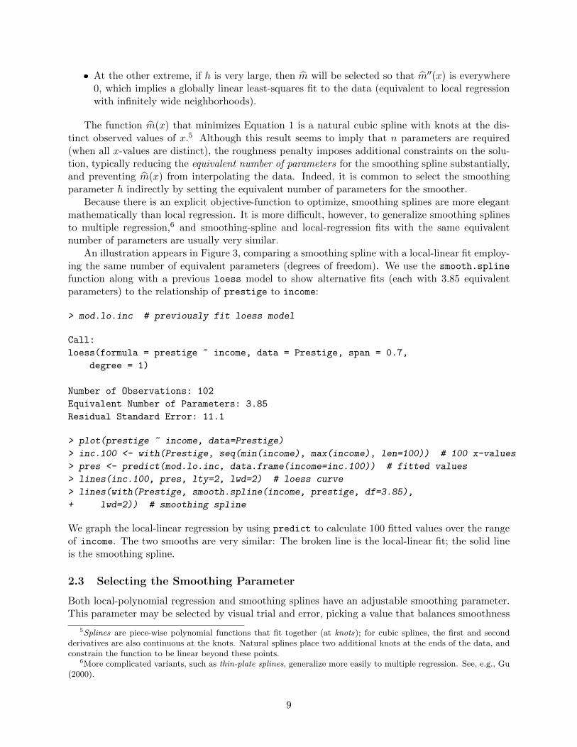
An illustration appears in Figure 3, comparing a smoothing spline with a local-linear fit employ-ing the same number of equivalent parameters (degrees of freedom). We use the smooth.spline

function along with a previous loess model to show alternative fits (each with 3.85 equivalentparameters) to the relationship of prestige to income:

> mod.lo.inc # previously fit loess model

Call:

loess(formula = prestige ˜ income, data = Prestige, span = 0.7,

degree = 1)

Number of Observations: 102

Equivalent Number of Parameters: 3.85

Residual Standard Error: 11.1

> plot(prestige ˜ income, data=Prestige)

> inc.100 <- with(Prestige, seq(min(income), max(income), len=100)) # 100 x-values

> pres <- predict(mod.lo.inc, data.frame(income=inc.100)) # fitted values

> lines(inc.100, pres, lty=2, lwd=2) # loess curve

> lines(with(Prestige, smooth.spline(income, prestige, df=3.85),

+ lwd=2)) # smoothing spline

We graph the local-linear regression by using predict to calculate 100 fitted values over the rangeof income. The two smooths are very similar: The broken line is the local-linear fit; the solid lineis the smoothing spline.

2.3 Selecting the Smoothing Parameter

Both local-polynomial regression and smoothing splines have an adjustable smoothing parameter.This parameter may be selected by visual trial and error, picking a value that balances smoothness

5Splines are piece-wise polynomial functions that fit together (at knots); for cubic splines, the first and secondderivatives are also continuous at the knots. Natural splines place two additional knots at the ends of the data, andconstrain the function to be linear beyond these points.

6More complicated variants, such as thin-plate splines, generalize more easily to multiple regression. See, e.g., Gu(2000).

9

● ●

●

●

●

●

●

●

●

●

●●

●

●

●

●

●

● ●

●

●

●

●

●

●●

●

●

●●

●

● ●

●

●

●

●

●

●

●●

●●●●

●

●

●●

●●

●

●

●

●●

●

●

●

●

●

●

●

●

●●

●

●

●

●

●

●

●

●

●

●●

●

●

●

●

●

●

●

●

●

●

●

● ●

●●

●

●

●

●

●

●

●●

●

●

0 5000 10000 15000 20000 25000

2040

6080

income

pres

tige

Figure 3: Local-regression (broken line) and smoothing-spline (solid line) fits for the regression ofprestige on income. Both models employ 3.85 equivalent parameters.

against fidelity to the data. More formal methods of selecting smoothing parameters typically tryto minimize the mean-squared error of the fit, either by employing a formula approximating themean-square error (e.g., so-called plug-in estimates), or by some form of cross-validation.

In cross-validation, the data are divided into subsets (possibly comprising the individual obser-vations); the model is successively fit omitting each subset in turn; and then the fitted model isused to ‘predict’ the response for the left-out subset. Trying this procedure for different values ofthe smoothing parameter will suggest a value that minimizes the cross-validation estimate of themean-squared error. Because cross-validation is very computationally intensive, approximationsand generalizations are often employed (see, e.g., Wood, 2000, 2004).

2.4 Additive Nonparametric Regression

The additive nonparametric regression model is

y = �0 +m1(x1) +m2(x2) + ⋅ ⋅ ⋅+mk(xk) + "

where the partial-regression functions mj are fit using a simple-regression smoother, such as localpolynomial regression or smoothing splines. We illustrate for the regression of prestige on income

and education, employing the gam function in the mgcv package (Wood, 2000, 2001, 2004, 2006):

> library(mgcv)

> mod.gam <- gam(prestige ˜ s(income) + s(education), data=Prestige)

> summary(mod.gam)

Family: gaussian

Link function: identity

10

Formula:

prestige ˜ s(income) + s(education)

Parametric coefficients:

Estimate Std. Error t value Pr(>|t|)

(Intercept) 46.833 0.689 68 <2e-16

Approximate significance of smooth terms:

edf Ref.df F p-value

s(income) 3.12 3.88 15.3 1.7e-09

s(education) 3.18 3.95 38.8 < 2e-16

R-sq.(adj) = 0.836 Deviance explained = 84.7%

GCV score = 52.143 Scale est. = 48.414 n = 102

The s function, used in specifying the model formula, indicates that each term is to be fit with asmoothing spline. The degrees of freedom for each term are found by generalized cross validation:7

In this case, the equivalent of 3.118 parameters are used for the income term, and 3.177 for theeducation term; the degrees of freedom for the model are the sum of these plus 1 for the regressionconstant.

The additive regression surface is plotted in Figure 4:

> fit.prestige <- matrix(predict(mod.gam, newdata), 25, 25)

> persp(inc, ed, fit.prestige, theta=45, phi=30, ticktype="detailed",

+ xlab="Income", ylab="Education", zlab="Prestige", expand=2/3,

+ shade=0.5)

The data frame newdata, used to find predicted values on the regression surface, was calculatedearlier to draw Figure 2 (page 7) for the general nonparametric multiple-regression model fit to thesedata. The two fits are quite similar. Moreover, because slices of the additive-regression surface inthe direction of one predictor (holding the other predictor constant) are parallel, it suffices to grapheach partial-regression function separately. This is the practical virtue of the additive-regressionmodel: It reduces a multidimensional (in this case, only three-dimensional) regression problem toa series of two-dimensional partial-regression graphs. The plot method for gam objects producesthese graphs, showing a point-wise 95-percent confidence envelope around the fit (Figure 5):

> plot(mod.gam)

Press return for next page....

The gam function is considerably more general than this example illustrates:

7The smoothing parameters are estimated along with the rest of the model, minimizing the generalized cross-validation criterion,

n�2

n− dfmod

where �2 is the estimated error variance and dfmod is the equivalent degrees of freedom for the model, includingboth parametric and smooth terms. In the generalized additive model (considered below) the estimated dispersion �replaces the estimated error variance.

11

Income

500010000

15000

20000

25000

Educa

tion

8

10

1214

Prestige

20

40

60

80

Figure 4: Fitted surface for the additive nonparametric regression of prestige on income andeducation.

0 5000 10000 15000 20000 25000

−20

−10

010

20

income

s(in

com

e,3.

12)

6 8 10 12 14 16

−20

−10

010

20

education

s(ed

ucat

ion,

3.18

)

Figure 5: Partial-regression functions for the additive regression of prestige on income and edu-

cation. The broken lines give point-wise 95-percent confidence envelopes around the fit.

12

� The model can include smooth (interaction) terms in two or more predictors, for example, ofthe form s(income, education).

� The model can be semi-parametric, including linear terms — for example, prestige ˜

s(income) + education.

� Certain technical options, such as the kinds of splines employed, may be selected by the user,and the user can fix the degrees of freedom for smooth terms.

� As its name implies (GAM = generalized additive model), the gam function is not restrictedto models with normal errors and an identity link (see below).

Hastie and Tibshirani’s (1990) gam function in the gam package predates and differs from thegam function in the mgcv package: First, it is possible to fit partial-regression functions by localpolynomial regression, using the lo function in a model formula, as well as by smoothing splines,using s. Second, the smoothing parameter for a term (the span for a local regression, or the degreesof freedom for a smoothing spline) is specified directly rather than determined by generalized cross-validation. As in the mgcv package, the gam function in the gam package can also fit generalizedadditive models.

3 Generalized Nonparametric Regression

We will illustrate generalized nonparametric regression by fitting a logistic semiparametric additiveregression model to Mroz’s labor-force participation data (described in Chapter 5, and included inthe car package). Recall that the response variable in this data set, lfp, is a factor coded yes forwomen in the labor-force, and no for those who are not. The predictors include number of childrenfive years of age or less (k5); number of children between the ages of six and 18 (k618); the woman’sage, in years; factors indicating whether the woman (wc) and her husband (hc) attended college,yes or no; and family income (inc), excluding the wife’s income and given in $1000s. We ignorethe remaining variable in the data set, the log of the wife’s expected wage rate, lwg; as explainedin the text, the peculiar definition of lwg makes its use problematic.

Because k5 and k618 are discrete, with relatively few distinct values, we will treat these predic-tors as factors, modeling them parametrically, along with the factors wc and hc; as well, becausethere are only three individuals with three children under 5, and only three with more than fivechildren between 6 and 18, we use the recode function in the car package to recode these unusualvalues:

> remove(list=objects()) # clean up everything

> Mroz$k5f <- factor(Mroz$k5)

> Mroz$k618f <- factor(Mroz$k618)

> Mroz$k5f <- recode(Mroz$k5f, "3 = 2")

> Mroz$k618f <- recode(Mroz$k618f, "6:8 = 5")

> mod.1 <- gam(lfp ˜ s(age) + s(inc) + k5f + k618f + wc + hc,

+ family=binomial, data=Mroz)

> summary(mod.1)

Family: binomial

Link function: logit

13

Formula:

lfp ˜ s(age) + s(inc) + k5f + k618f + wc + hc

Parametric coefficients:

Estimate Std. Error z value Pr(>|z|)

(Intercept) 0.542 0.180 3.01 0.0026

k5f1 -1.521 0.251 -6.07 1.3e-09

k5f2 -2.820 0.500 -5.64 1.7e-08

k618f1 -0.342 0.227 -1.51 0.1316

k618f2 -0.279 0.248 -1.12 0.2608

k618f3 -0.333 0.284 -1.17 0.2415

k618f4 -0.531 0.440 -1.21 0.2269

k618f5 -0.491 0.609 -0.81 0.4206

wcyes 0.980 0.223 4.39 1.1e-05

hcyes 0.159 0.206 0.77 0.4422


edf Ref.df Chi.sq p-value

s(age) 1.67 2.09 26.2 2.4e-06

s(inc) 1.74 2.19 17.5 0.00020

R-sq.(adj) = 0.128 Deviance explained = 10.9%

UBRE score = 0.25363 Scale est. = 1 n = 753

Summarizing the gam object shows coefficient estimates and standard errors for the parametric partof the model; the degrees of freedom used for each smooth term (in the example, for age and inc),and a significance test for the term; and several summary statistics, including the UBRE score forthe model.8

The anova function applied to a single gam object reports Wald tests for the terms in the model:

> anova(mod.1)

Family: binomial

Link function: logit

Formula:

lfp ˜ s(age) + s(inc) + k5f + k618f + wc + hc

Parametric Terms:

df Chi.sq p-value

k5f 2 55.61 8.4e-13

k618f 5 3.28 0.66

wc 1 19.26 1.1e-05

hc 1 0.59 0.44


8For a binomial model, by default gam minimizes the UBRE (unbiased risk estimator) criterion (Wahba, 1990) inplace of the GCV criterion.

14

30 35 40 45 50 55 60

−3

−2

−1

01

age

s(ag

e,1.

67)

0 20 40 60 80

−3

−2

−1

01

inc

s(in

c,1.

74)

Figure 6: Smooth terms for age and inc in a semi-parametric generalized additive model for Mroz’slabor-force participation data.

edf Ref.df Chi.sq p-value

s(age) 1.67 2.09 26.2 2.4e-06

s(inc) 1.74 2.19 17.5 0.00020

The plot method for gam objects graphs the smooth terms in the model, along with point-wise95-percent confidence envelopes (Figure 6):

> plot(mod.1)

Press return for next page....

The departures from linearity are not great. Moreover, the regression function for inc is veryimprecisely estimated at the right, where data values are sparse, and we would probably have donewell do transform inc by taking logs prior to fitting the model.

One use of additive regression models, including generalized additive models, is to test for nonlin-earity: We may proceed by contrasting the deviance for a model that fits a term nonparametricallywith the deviance for an otherwise identical model that fits the term linearly. To illustrate, wereplace the smooth term for age in the model with a linear term:

> mod.2 <- gam(lfp ˜ age + s(inc) + k5f + k618f + wc + hc,


> anova(mod.2, mod.1, test="Chisq")

Analysis of Deviance Table

Model 1: lfp ˜ age + s(inc) + k5f + k618f + wc + hc

Model 2: lfp ˜ s(age) + s(inc) + k5f + k618f + wc + hc

Resid. Df Resid. Dev Df Deviance P(>|Chi|)

1 740 919

2 740 917 0.72 2.21 0.09

15

Likewise, we can test for nonlinearity in the inc (income) effect:

> mod.3 <- gam(lfp ˜ s(age) + inc + k5f + k618f + wc + hc,




Model 1: lfp ˜ s(age) + inc + k5f + k618f + wc + hc



1 740 920

2 740 917 0.783 2.55 0.08

Neither test is quite statistically significant.9

Similarly, we can test the statistical significance of a term in the model by dropping it andnoting the change in the deviance. For example, to test the age term:

> mod.4 <- update(mod.1, . ˜ . - s(age))



Model 1: lfp ˜ s(inc) + k5f + k618f + wc + hc



1 741 945

2 740 917 1.48 27.5 4.2e-07

Thus, the age effect is very highly statistically significant.10 Compare this with the similar resultfor the Wald test for age, presented above. We leave it to the reader to perform similar tests forthe other predictors in the model, including inc and the parametric terms.

4 Complementary Reading and References

Nonparametric regression is taken up in Fox (2008, Chap. 18).All of the nonparametric regression models discussed in this appendix (and some others, such as

projection-pursuit regression, and classification and regression trees) are described in Fox (2000b,a),from which the examples appearing in the appendix are adapted.

The excellent and wide-ranging books by Hastie and Tibshirani (1990) and Wood (2006) areassociated respectively with the gam and mgcv packages, the latter a part of the standard Rdistribution. A briefer treatment of GAMs and the gam function in the gam package appears in apaper by Hastie (1992).

9We invite the reader to perform tests for nonlinearity for the factors k5f and k618f.10Applied to models in which the degree of smoothing is selected by GCV or UBRE, rather than fixed, these tests

tend to exaggerate the statistical significance of terms in the model.

16

References

Bowman, A. W. and Azzalini, A. (1997). Applied Smoothing Techniques for Data Analysis: TheKernel Approach With S-Plus Illustrations. Oxford University Press, Oxford.

Fox, J. (2000a). Multiple and Generalized Nonparametric Regression. Thousand Oaks, CA.

Fox, J. (2000b). Nonparametric Simple Regression: Smoothing Scatterplots. Thousand Oaks, CA.

Fox, J. (2008). Applied Regression Analysis and Generalized Linear Models. Sage, Thousand Oaks,CA, second edition.

Fox, J. and Weisberg, S. (2011). An R Companion to Applied Regression. Sage, Thousand Oaks,CA, second edition.

Gu, C. (2000). Multidimensional smoothing with smoothing splines. In Schmiek, M. G., editor,Smoothing and Regression: Approaches, Computation, and Applications. Wiley, New York.

Hastie, T. J. (1992). Generalized additive models. In Chambers, J. M. and Hastie, T. J., editors,Statistical Models in S, pages 421–454. Wadsworth, Pacific Grove, CA.

Hastie, T. J. and Tibshirani, R. J. (1990). Generalized Additive Models. Chapman and Hall,London.

Loader, C. (1999). Local Regression and Likelihood. Springer, New York.

Nason, G. (2008). Wavelet Methods in Statistics with R. New York.

Nason, G. P. and Silverman, B. W. (1994). The discrete wavelet transform in S. Journal ofComputational and Graphical Statistics, 3:163–191.

Nason, G. P. and Silverman, B. W. (2000). Wavelets for regression and other statistical problems. InSchmiek, M. G., editor, Smoothing and Regression: Approaches, Computation, and Applications.Wiley, New York.

Wahba, G. (1990). Spline Models for Observational Data. SIAM, Philadelphia.

Wood, S. N. (2000). Modelling and smoothing parameter estimation with multiple quadratic penal-ties. Journal of the Royal Statistical Socieity, Series B, 62:413–428.

Wood, S. N. (2001). mgcv: GAMS and generalized ridge regression for R. R News, 1(2):20–25.

Wood, S. N. (2004). Stable and efficient multiple smoothing parameter estimation for generalizedadditive models. Journal of the American Statistics Association, 99:673–686.

Wood, S. N. (2006). Generalized Additive Models: An Introduction with R. Chapman and Hall,Boca Raton, FL.

17

nonparametric regression in r - faculty of social … regression in r ... nonparametric regression,...

Documents