N5-1

Note 05 AC Circuits II: Steady State SignalsIn this note we examine the response of an AC circuit to a steady state signal. We expand our study toinclude circuits composed of two and three elements. We shall see that a circuit comprised of a capacitor-resistor combination, an inductor-resistor combination, or of all three elements behaves, electrically, like afrequency selective attenuator, or filter. We use complex number notation throughout.

Basic Model of a FilterWe have seen in an earlier note how a voltage dividercan be made from two resistors in series. The equiva-lent AC circuit is one with two impedances Z1 and Z2in series (Figure 5-1). This circuit is not known as animpedance divider, but rather as a signal filter, as weshall show.

€

vin (t)

€

vout (t)€

Z1

€

Z2€

i (t)

Figure 5-1. A voltage divider consisting of two impedancesin series serves as the general model of a filter.

This circuit has an input voltage vin provided, per-haps, by a signal generator or a previous stage (on theleft) and an output voltage vout appearing across theimpedance Z2 (on the right). Ordinarily, a load or asubsequent stage would be connected across it. Forconvenience we assume that the impedance of theload is so high that the current drawn by the load isnegligible. A common current i(t) flows around theloop.

In what follows we shall wish to reference thephases of signals to the phase of the input voltage. Wetherefore set vin’s intrinsic phase constant to zero andwrite the voltages and current as 1

€

vin (t) =Vinejωt ; vout (t) =Voute

j(ωt +φ )

…[5-1a, b, c]and

€

i(t) = Ie j(ωt +φ ' ) .

We understand that the physically meaningful volt-

1 We use j here for √-1 instead of the more common i to avoidconfusion with the symbol for current. We use the input voltage asreference for the simple reason that voltage, not current, signals getdisplayed on an oscilloscope.

ages and currents are the real parts of these quantities.We thus allow for i(t), vin(t) and vout(t) to have differentintrinsic phases. Applying KVR around the loop inFigure 5-1 we get

€

vin (t) = i(t)Z1 + i(t)Z2

so

€

Vinejωt = Z1 + Z2( )Ie j(ωt +φ ' ) …[5-2]

and

€

vout (t) = i(t)Z2

so

€

Voutej(ωt +φ ) = Z2Ie

j(ωt+φ ' ) . …[5-3]

Dividing eq[5-3] by eq[5-2] we get

€

Vout

Vin

e jφ =Z2

Z1 + Z2 . …[5-4]

The left hand side of eq[5-4] is the product of twofactors. We can write the first factor as:

€

Vout

Vin

=Vout( )pkVin( )pk

=Vout( )pk− pkVin( )pk− pk

=Vout( )rmsVin( )rms

The peak, peak-to-peak or rms values are what can bemeasured with an AC voltmeter or oscilloscope. Thesecond factor, ejφ, is called the phase factor, where φ(ω)is the angle the output voltage leads the input voltage.

In electronics parlance, eq[5-4] is called the transferfunction of the circuit. It is, of course, complex. It iscommonly denoted H(jω) with a complex argument toremind us of its complex nature. Thus

€

H( jω) =Vout

Vin

e jφ = H( jω)e jφ . …[5-5]

Since H(jω) is complex we can write it in the usualforms for complex numbers:

€

H( jω) = Re H( jω)[ ] + j Im H( jω)[ ]

Note 05

N5-2

€

= Re H( jω)[ ]( )2 + Im H( jω)[ ]( )2e jφ

where

€

tanφ(ω) =Im H( jω)[ ]Re H( jω)[ ]

. …[5-6]

In the event that Z 1 and Z 2 are known algebraically,we can compute H(jω) from

€

H( jω) =Z2

Z1 + Z2. …[5-7]

We shall return to complex numbers in a moment. It isworthwhile now to actually show how |H(jω)|andφ(ω) might be measured with an oscilloscope.

Example Problem 5-1Measuring |H(jω)| and φ(ω) on an Oscilloscope

The voltage signal applied to a filter, and the outputsignal taken from the filter, are shown in Figure 5-2.The input is applied to CH1, the output to CH2.Calculate the absolute value of the transfer function ofthe filter and the angle the output voltage leads (orlags) the input voltage.

Figure 5-2. The input and output voltages of a filter.

Solution:You can see from the measurement boxes down theright hand side of the display that the oscilloscope hasmeasured the output and input Pk-Pk voltages as 178mV and 520 mV, respectively. Thus

€

H( jω) =178 mV520 mV

= 0.34 .

If you examine the screen carefully you can see thatone period of the waveform (950.0 µs) covers about 9small time divisions along the center of the display.Thus

€

9 time div ≡ 950.0 µs

so

€

1 time div =950.0

9≡105.6 µs .

If you look more closely you can see that the timedifference between the two signals comes to about 1.5time div, which translates to 158.3 µs. We can calcul-ate the phase difference from eq[4-5]:

€

158.3950.0

=Δφ2π

,

which gives

€

Δφ =1.046 rad ≡ 60˚ .

Establishing which signal is the leading or lagging onetakes some knowledge of oscilloscope functionality.The oscilloscope was set to trigger on the CH1 signal(the usual choice). The trigger position is at the exactcenter of the screen. Therefore what appears to be thesmaller of the two signals (actually the larger becausethe signals are scaled differently) is the signal appliedto CH1. The CH2 signal goes through zero before theCH1 signal (reading “up” in time from the center ofthe screen) and is therefore the leading signal. There-fore the output voltage leads the input voltage by 60˚.We shall see later in this note that this fact ischaracteristic of an RC high-pass filter.

In passing it should be pointed out that a moreaccurate method of measuring a phase difference is touse the cursors on the oscilloscope. For an example ofthis see Figures 5-2 of Experiment 05, “Wave Filters”.

Preview of FiltersA filter is a “frequency selective” attenuator. It is usedto modify the frequency spectrum of a signal consis-ting of many component signals by attenuating somecomponents over a certain range of frequencies whileleaving others unaffected. A filter which provides noamplification (discussed here) is a passive filter. Weshall discuss active filters or amplifiers in Note 08. Afilter is commonly represented in general terms as afour terminal network (Figure 5-3). There are twoinput lines and two output lines, with one of the twolines often connected together and to ground.

Note 05

N5-3

(often common)

+ +

– –

vin vout

Figure 5-3. A four terminal network is a general model of afilter.

Sketches of the absolute value of H(jω) vs ω for fourtypes of filter are given in Figures 5-4.

ω ω

(a) (b)

1 H = voutvin

ω ω

(c) (d)

1

Figure 5-4. Sketches (a) through (d) show |H(jω)| vs ω fora low pass, high pass, band pass and band reject filter,respectively.

You should take a few moments to study the curves tounderstand what effect the filters have on an inputsignal. The filter described by Figure 5-4a passes thelow frequency components of the input signal whileattenuating the high frequency components. The filterdescribed by Figure 5-4d attenuates components in anarrow range or band, hence the name band rejectfilter.

The shape of the frequency response of |H(jω)| isdescribed by three parameters: 3 dB points, roll-off, andbandwidth. These parameters may be defined withreference to Figure 5-5 that shows a semi-log plot of|H(jω)| for a hypothetical band pass filter. Transferfunctions and phases are commonly plotted onsemilog graphs because ω can vary over many ordersof magnitude.

12

log ωω 2ω 1

H1

Figure 5-5. A semilog plot of |H(jω)| vs log10ω for a hypo-thetical band pass filter. This is also known as a Bode plot.

For this particular filter, |H(jω)| (and Vout/Vin) = 1/√2at the frequencies ω 1 and ω2. These frequencies, atwhich the power ratio Pout/Pin = 1/2, are called the“half-power” or 3 dB points. By definition, the freq-uency bandwidth bw is given by 2

€

bw =12π

ω2 −ω1( ) Hz, …[5-8]

expressed in linear frequency. Roll off is a measure ofthe steepness of the curve in those regions where thecurve is changing. In these regions

€

H( jω) ≈ω n ,

where n takes on the common values 1, 2, or 3 (forincreasing log|H(jω)|) or –1, –2 or –3 (for decreasinglog|H(jω)|). Thus we may write

€

# in dB = 20log10H2( jω)H1( jω)

= 20log10

ω2n

ω1n

€

= 20n log10ω2

ω1

,

where n is a parameter. Two values of the ratio ω2/ω1are the most useful: the octave when the ratio is 2, andthe decade when the ratio is 10. Thus the slope ofvarious regions of the transfer function where it ischanging can be described in terms of the number ofdB per octave or the number of dB per decade:

€

dB /octave = 20n log10(2) ≈ 6n 2 The specification of frequency response does vary among manu-facturers. For example, the frequency response of an FM tuner usedby the author is quoted as 30 Hz to 15 kHz at the ±1.5 dB points.

Note 05

N5-4

€

dB /decade = 20n log10(10) ≈ 20n .

A filter is said to “roll off by 6, 12, or 18 dB peroctave” corresponding to log-log slopes of 1, 2, or 3.Usually, the greater the roll off (and the steeper theslope) the more desireable the filter.

One example of a filter that you probably use everyday without knowing it is the crossover network thatis part of your audio system (it lies hidden inside thespeaker enclosure). A two-way crossover networkconsists of at least two filters, a low pass section and ahigh pass section. The woofer, or low frequencyspeaker, is connected to the low pass section terminalswhile the tweeter, the high frequency speaker, isconnected to the high pass section terminals. Othermore elaborate (and expensive) networks may consistof three or more sections.

Steady State ResponsesWe now return to the business of describing circuitswith complex numbers. A resistor and a capacitor, ora resistor and an inductor, arranged as a voltagedivider will serve as a low- or a high-pass filterdepending on which component is placed across theoutput (Z2 in Figure 5-1). We begin with the RC lowpass filter.

The RC Low Pass FilterAn RC circuit with the capacitor across the output issketched in Figure 5-6.

R Cvin vout

Figure 5-6. An RC low pass filter.

Using eq[5-7], the transfer function of this circuit isgiven by

€

H( jω) =ZC

ZR + ZC=

−j

ωCR − j

ωC

€

=1

1+ jωRC. …[5-9]

We are interested in finding the magnitude and phase

factor of this expression. Two methods will give theresults: the cartesian method and the polar method. In aparticular problem you may find one method easier towork out than the other. In either method the basicstrategy is to convert the complex number (often inthe form of a ratio) to an expression of the form a + jbwhere a and b are reals.

Cartesian MethodThis method consists of multiplying the numeratorand the denominator by the complex conjugate of thedenominator. That done you then simplify the expres-sion and find the magnitude and phase factor. Toillustrate, we have for eq[5-9]:

€

H( jω) =1

1+ jωRC×1− jωRC1− jωRC

€

=1− jωRC1+ω 2R2C2 ,

€

=1+ω 2R2C2

1+ω 2R2C2 e jφ

€

=1

1+ω 2R2C2e jφ .

Thus

€

H( jω) = H( jω)e jφ , …[5-10]

where

€

tanφ(ω) =−ωRC1

. …[5-11a]

and

€

H( jω) =1

1+ω 2R2C2. …[5-11b]

Polar MethodTo apply the polar method we use the fact that

€

H( jω) =| numerator | × e jφn

| denominator | × e jφd

€

=numeratordenominator

e j φn−φd( ) ,

where φn and φd are the phase angles of the complexnumerator and denominator, respectively. Thus foreq[5-9]:

Note 05

N5-5

€

H( jω) =1

1+ω 2R2C2e j φn−φ d( ) ,

where

€

φn = tan−1(0) = 0,

and

€

φd = tan−1 ωRC1

.

Thus it follows that

€

φ(ω) = tan−1 −ωRC1

. …[5-12a]

and

€

H( jω) =1

1+ω 2R2C2e jφ , …[5-12b]

which agree with eqs[5-11]. Applied with care thepolar method is very often the easier of the twomethods to work with.

Plotting the FunctionsHaving used either method we need to plot |H(jω)|and φ(ω) vs ω. Taking limits is a good place to start.We first find the limits of eqs[5-11a and b]:

As ω → 0, |H(jω)|→ 1, tanφ → 0, φ→0,

as ω → ∞, |H(jω)|→ 0, tanφ → –∞, φ→–π/2,

|H(jω)| takes the following approximate, but useful,forms at low frequency and high frequency:

€

H( jω) low =1 and H( jω) high =1

ωRC.

Thus at low frequencies, |H(jω)| tends to unity, whileat high frequencies |H(jω)| decreases as 1/ω withslope 1/RC (Figure 5-7a).

The frequency at which |H(jω)|low = |H(jω)|high iscalled the corner frequency and denoted ωC. In this case

€

ωC =1RC

(rad.s–1).

The corner frequency is the same frequency at which|H(jω)| = 1/√2. The bandwidth (in rad.s–1) extendsfrom 0 to ωC; expressed in Hz it is bw = 1/(2πRC) Hz.Beyond ωC the roll off is 6 dB per octave.

You should be able to work out the effect of the filteron the applied signal from the graphs. At low freq-

uencies, the output signal is neither attenuated norphase shifted with respect to the input. But at higherfrequencies beyond ωC, the output is attenuatedrelative to the input and is shifted in phase. Theoutput lags the input. It can be shown that at highfrequencies the output signal is in fact proportional tothe integral of the input, a result that can be useful.

(a)

(b)Figure 5-7. Plots of |H(jω)| and φ(ω) vs log10ω for an RClow-pass filter consisting of C = 1.0 µF and R = 100 Ω . Atthe corner frequency |H(jω)| is reduced to 1/√2 and theoutput lags the input by π /4 radians (45 degrees).

As you might expect, if the output of an RC filter istaken across the resistor instead of across the capacitor(Figure 5-6) the circuit becomes a high pass filter.

Note 05

N5-6

The RL Low Pass FilterRC and RL circuits respond to AC signals in similar,complementary ways. If possible, a filter is usuallyconstructed from an RC circuit since capacitors arecheaper and more nearly ideal than are inductors.Inductive filters are found today most often in powersupplies and in special applications like cross-overnetworks.

An RL circuit with the resistor connected across theoutput is shown in Figure 5-8. It too can be shown tobe a low pass filter.

R L

vin vout

Figure 5-8. An RL low pass filter.

The transfer function of this circuit is given by

€

H( jω) =ZR

ZR + ZL

=R

R + jωL

€

=R

R + jωL×R − jωLR − jωL

€

=R

R2 +ω 2L2

(R − jωL) .

Thus

€

H( jω) =R

R2 +ω 2L2

R2 +ω 2L2( )

1/ 2e jφ ,

€

=R

R2 +ω 2L2e jφ , …[5-13]

where

€

tanφ(ω) = −ωLR

. …[5-14a]

and

€

H( jω) =1

1+ω 2L2

R2

…[5-14b]

Taking the limits of eqs[5-14], we have:

As ω → 0, |H(jω)|→ 1, tanφ → 0, φ→0,

and ω → ∞, |H(jω)|→ 0, tanφ → –∞, φ→–π/2.

At low and high frequencies |H(jω)|reduces to usefulapproximate forms. These are:

€

H( jω) low =1 and H( jω) high =RωL

.

The corner frequency is

€

ωC =RL

.

Plots of |H(jω )|and φ(ω ) vs log10ω are given inFigures 5-9. The bw factor, 3 dB points and roll off canbe obtained as described in previous sections.

As you might expect, if the output of the RL circuit istaken across the inductor instead of across the resistor(Figure 5-8), the circuit becomes a high pass filter.

(a)

(b)Figure 5-9. Plots of |H(jω)| and φ(ω) vs log10ω for an RLlow pass filter.

Note 05

N5-7

The Series RCL FilterThe steady state response of a circuit consisting of aresistor, a capacitor and an inductor connected inseries exhibits some of the effects of the RC and RLcircuits just described. We shall see that this kind ofcircuit passes signals with frequencies in a range or aband. Thus the circuit is called a band-pass filter. Thisaction results from an effect called resonance.

A series RCL circuit is drawn in Figure 5-10. We canfind its transfer function by extending the treatmentsof the previous examples.

R

L

Cvin vout

Figure 5-10. A series RCL circuit with the resistor connectedacross the output forms a band-pass filter.

Since the elements are in series and the resistor isacross the output we have

€

H( jω) =ZR

ZR + ZL + ZC=

R

R + jωL − jωC

€

=R

R + j ωL − 1ωC

×R − j ωL − 1

ωC

R − j ωL − 1ωC

€

=R

R2 + ωL − 1ωC

2e jφ …[5-15]

where

€

tanφ(ω) =− ωL − 1

ωC

R…[5-16a]

and

€

H( jω) =R

R2 + ωL − 1ωC

2

…[5-16b]

Taking the limits of eqs[5-16], we have:

As ω → 0, |H(jω)|→ 0, tanφ → ∞, φ→π/2,

and ω → ∞, |H(jω)|→ 0, tanφ → –∞, φ→–π/2.

At low frequencies and again at high frequencies|H(jω)| reduces to the useful, approximate forms:

€

H( jω) low =ωRC and H( jω) high =RωL

,

(or |H(jω)|low ≈ ω1 and |H(jω )|high ≈ ω –1). The 3dBpoints or the frequencies at which |H(jω)|= 1/√2, arethe frequencies for which ωL – 1/ωC = ±R . At thefrequency

€

ω0 =1LC

. …[5-17]

the factor involving ω in eqs[5-16] vanishes. At thisfrequency,

€

H( jω0) =1 and φ(ω0) = 0 .

At the special frequency ω0 the capacitive and induc-tive impedances are equal and add to zero. ω0 is calledthe resonance frequency or the natural frequency of oscilla-tions. At this frequency the output voltage appearingacross R equals the input voltage (|H(jω)|= 1), and isunshifted in phase. |H(jω )| and φ(ω) vs log10ω aresketched in Figures 5-11.

You should be able to identify the band pass natureof the filter from the sketches. At both low and highfrequencies the output signal is both attenuated andphase shifted with respect to the input. Only at thereson-ance frequency is the input signal passed to theout-put without attenuation or phase shifting. It isuseful to quantify the shape of the bandpass in orderto differentiate between one filter and another. Thesharpness of the curve near the frequency ω0 in Figure5-11a is described by the 3 dB point and the Q factor,with the latter defined:

€

Q =ω0LR

=1

ω0RC.

Note 05

N5-8

ω 0

logω

(a) slope = 1

slope = –1

1 3 dB points1

2

log H

φ

0

π/2

(b)

ω –π/2

ω0 = 1LC

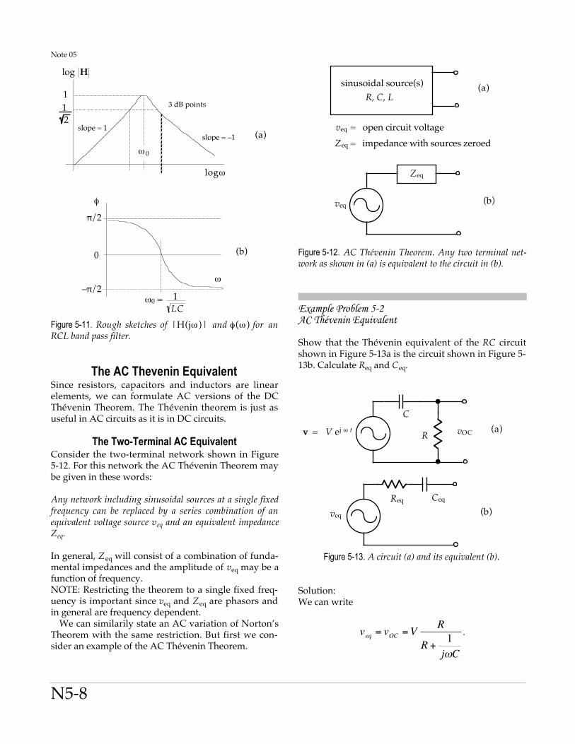
Figure 5-11. Rough sketches of |H(jω )| and φ(ω) for anRCL band pass filter.

The AC Thevenin EquivalentSince resistors, capacitors and inductors are linearelements, we can formulate AC versions of the DCThévenin Theorem. The Thévenin theorem is just asuseful in AC circuits as it is in DC circuits.

The Two-Terminal AC EquivalentConsider the two-terminal network shown in Figure5-12. For this network the AC Thévenin Theorem maybe given in these words:

Any network including sinusoidal sources at a single fixedfrequency can be replaced by a series combination of anequivalent voltage source veq and an equivalent impedanceZeq.

In general, Zeq will consist of a combination of funda-mental impedances and the amplitude of veq may be afunction of frequency.NOTE: Restricting the theorem to a single fixed freq-uency is important since veq and Zeq are phasors andin general are frequency dependent.

We can similarily state an AC variation of Norton’sTheorem with the same restriction. But first we con-sider an example of the AC Thévenin Theorem.

(a) sinusoidal source(s) R, C, L

= open circuit voltage = impedance with sources zeroed

veq

Zeq

veq

Zeq

(b)

Figure 5-12. AC Thévenin Theorem. Any two terminal net-work as shown in (a) is equivalent to the circuit in (b).

Example Problem 5-2AC Thévenin Equivalent

Show that the Thévenin equivalent of the RC circuitshown in Figure 5-13a is the circuit shown in Figure 5-13b. Calculate Req and Ceq.

C

R (a)v = V ej ω t vOC

(b)veq

Req Ceq

Figure 5-13. A circuit (a) and its equivalent (b).

Solution:We can write

€

veq = vOC =V R

R +1jωC

.

Note 05

N5-9

If the source is zeroed, then C and R appear inparallel. Therefore

€

Zeq =R × 1

jωC

R +1jωC

=R

1+ jωRC.

To find the magnitude and phase of veq we write

€

veq =V jωRC1+ jωRC

=V ωRC1+ω 2R2C2

e jφ

where

€

tanφ =1

ωRC.

We can also express Zeq as a sum of a real and animaginary term:

€

Zeq =R

1+ jωRC=R(1− jωRC)1+ω 2R2C2

€

=R

1+ω 2R2C2 − jωR2C

1+ω 2R2C2

€

= Req − j1

ωCeq

,

where

€

Req =R

1+ω 2R2C2

and

€

Ceq =1+ω 2R2C2

ω 2R2C.

The equivalent circuit is therefore as shown in Figure5-13b. Let us now look at a numerical example.

Example Problem 5-3AC Thévenin Equivalent: A Worked Example

Show that the circuit of Figure 5-14a is equivalent tothe circuit of Figure 5-14b at f = 60 Hz if R = 1 kΩ andC = 1 µF.

(a) 1 µF

f = 60 Hz

v 103 Ω

(b)

f = 60 Hz

0.3528V

876 Ω

8.04 µF

Figure 5-14.The circuit in (b) is the Thévenin equivalent ofthe circuit in (a).

Solution:At f = 60 Hz, ω = 2π f = 377 s–1 and ωRC = 0.377

we have veqv = 0.377

1 + 0.3772 1/2 = 0.3528 ,

and Tan φ = 10.377

so that φ = 69.35 .

Thus Req = 103

1 + 0.3772 = 876 Ω ,

and Ceq = 1 + 0.3772

0.3772 = 8.04 µF .

Thus the equivalent circuit is, indeed, the circuitsketched in Figure 5-14b.

Note 05

N5-10

AppendixA Guide for Using Oscar

Oscar is an application developed to control Tek TDS2xx/1xxx series digital oscilloscopes (Figure A-1). It wasbuilt at UTSC with the LabVIEW development system. The program makes it possible to control the oscilloscopefrom a computer, to transfer data to the computer, to plot waveforms and analyze waveforms. Our objective hereis to survey enough of the functionality of the program to enable you to use it in experiments.

Figure A-1. The panel of Oscar at the time of writing. A sinewave at a frequency of about 1 kHz is plotted in a YT SingleGraph. On bootup Channel 2 on the oscilloscope was OFF (shown in red on a color monitor). The display of the oscilloscopeappeared as is reproduced in Figure A-2.

Figure A-2. The display of the oscilloscope when Oscar wasbooted and produced the panel shown in Figure A-1.

First BootOscar was designed to interrogate the oscilloscope onbootup and to transfer its data from both channelsautomatically. It works transparently with serial RS-232 or GPIB interfaces. This means that before bootingthe program you should:

• Ensure that a serial cable connects the RS-232 con-nector on the rear of your oscilloscope with theCOM1 (modem) port of your computer. Alternat-ively, if you are using the GPIB interface, check tosee that a GPIB cable is properly connected.

• Manipulate the front panel of your oscilloscopeand external components, signal generator and soforth, to display the waveform on your oscillo-scope whose data or display you wish to transfer.

• Ensure that the monitor on your computer is set

Note 05

N5-11

for a screen size of at least 1024 x 768 pixels, orelse Oscar will not run as intended

• An alias for Oscar should be visible on the desk-top of your computer. Run Oscar by double-clicking the alias. The program should transfer thedata of whatever waveform(s) is (are) currentlybeing displayed in about 20 seconds. Whenrunning, Oscar’s panel should resemble Figure A-1. The data transferred are listed in the middlebottom of the Panel. You might wish to compareOscar’s panel with the display of your oscilloscopeto spot their similarities and differences.

Oscar’s panel was deliberately designed to resemble

the display of the Tek TDS2xx/1002 series oscillo-scopes. The area for the graph is bordered by variousmeasurements arrayed in more or less the same rela-tive position as they appear on the computer display.Numbers appearing in the “measurement boxes” (theblack rectangles) down the right hand side of thegraph area have been transferred from the oscillo-scope. Other numbers on the Panel have been calcula-ted by Oscar. At this stage you can scan the menubar(Figure A-3) to get an idea of Oscar’s functionality. Wediscuss a selection of these items that should be ofmost interest to you.

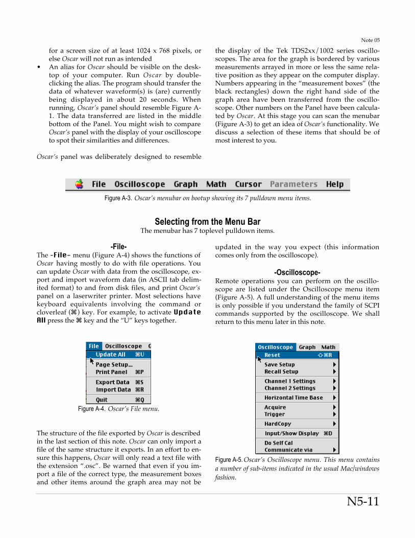
Figure A-3. Oscar’s menubar on bootup showing its 7 pulldown menu items.

Selecting from the Menu BarThe menubar has 7 toplevel pulldown items.

-File-The –File- menu (Figure A-4) shows the functions ofOscar having mostly to do with file operations. Youcan update Oscar with data from the oscilloscope, ex-port and import waveform data (in ASCII tab delim-ited format) to and from disk files, and print Oscar’spanel on a laserwriter printer. Most selections havekeyboard equivalents involving the command orcloverleaf () key. For example, to activate UpdateAll press the key and the “U” keys together.

Figure A-4. Oscar’s File menu.

The structure of the file exported by Oscar is describedin the last section of this note. Oscar can only import afile of the same structure it exports. In an effort to en-sure this happens, Oscar will only read a text file withthe extension “.osc”. Be warned that even if you im-port a file of the correct type, the measurement boxesand other items around the graph area may not be

updated in the way you expect (this informationcomes only from the oscilloscope).

-Oscilloscope-Remote operations you can perform on the oscillo-scope are listed under the Oscilloscope menu item(Figure A-5). A full understanding of the menu itemsis only possible if you understand the family of SCPIcommands supported by the oscilloscope. We shallreturn to this menu later in this note.

Figure A-5. Oscar’s Oscilloscope menu. This menu containsa number of sub-items indicated in the usual Mac/windowsfashion.

Note 05

N5-12

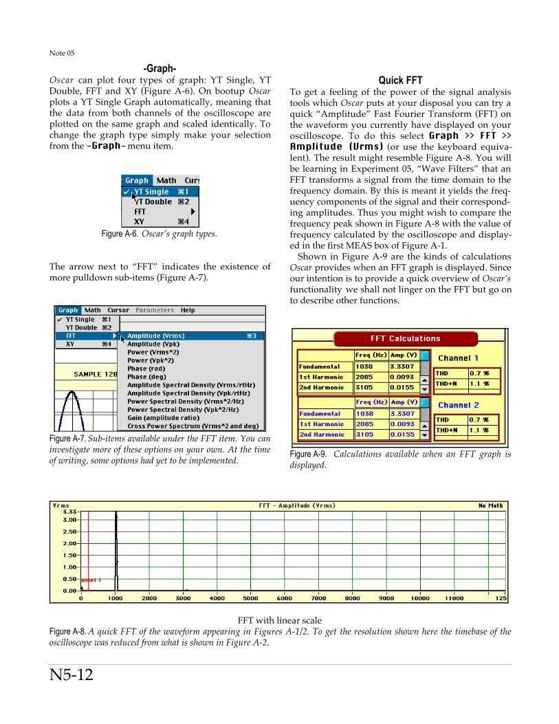
-Graph-Oscar can plot four types of graph: YT Single, YTDouble, FFT and XY (Figure A-6). On bootup Oscarplots a YT Single Graph automatically, meaning thatthe data from both channels of the oscilloscope areplotted on the same graph and scaled identically. Tochange the graph type simply make your selectionfrom the -Graph- menu item.

Figure A-6. Oscar’s graph types.

The arrow next to “FFT” indicates the existence ofmore pulldown sub-items (Figure A-7).

Figure A-7. Sub-items available under the FFT item. You caninvestigate more of these options on your own. At the timeof writing, some options had yet to be implemented.

Quick FFTTo get a feeling of the power of the signal analysistools which Oscar puts at your disposal you can try aquick “Amplitude” Fast Fourier Transform (FFT) onthe waveform you currently have displayed on youroscilloscope. To do this select Graph >> FFT >>Amplitude (Vrms) (or use the keyboard equiva-lent). The result might resemble Figure A-8. You willbe learning in Experiment 05, “Wave Filters” that anFFT transforms a signal from the time domain to thefrequency domain. By this is meant it yields the freq-uency components of the signal and their correspond-ing amplitudes. Thus you might wish to compare thefrequency peak shown in Figure A-8 with the value offrequency calculated by the oscilloscope and display-ed in the first MEAS box of Figure A-1.

Shown in Figure A-9 are the kinds of calculationsOscar provides when an FFT graph is displayed. Sinceour intention is to provide a quick overview of Oscar’sfunctionality we shall not linger on the FFT but go onto describe other functions.

Figure A-9. Calculations available when an FFT graph isdisplayed.

FFT with linear scaleFigure A-8. A quick FFT of the waveform appearing in Figures A-1/2. To get the resolution shown here the timebase of theoscilloscope was reduced from what is shown in Figure A-2.

Note 05

N5-13

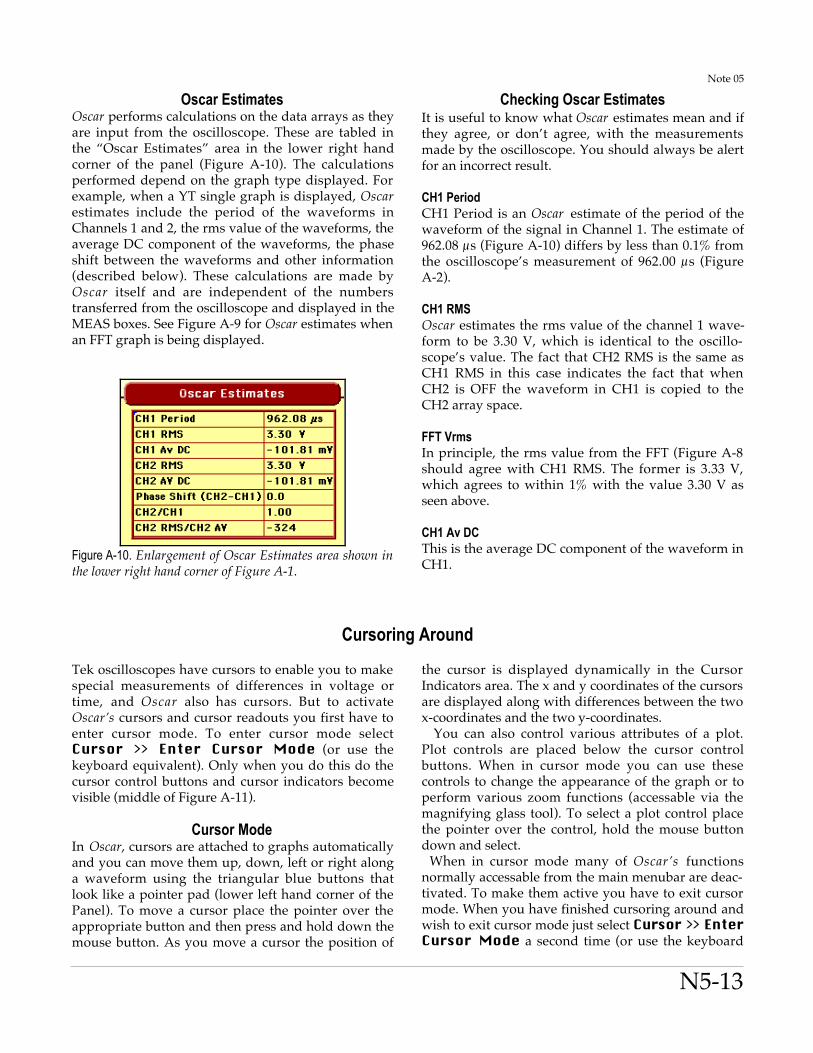
Oscar EstimatesOscar performs calculations on the data arrays as theyare input from the oscilloscope. These are tabled inthe “Oscar Estimates” area in the lower right handcorner of the panel (Figure A-10). The calculationsperformed depend on the graph type displayed. Forexample, when a YT single graph is displayed, Oscarestimates include the period of the waveforms inChannels 1 and 2, the rms value of the waveforms, theaverage DC component of the waveforms, the phaseshift between the waveforms and other information(described below). These calculations are made byOscar itself and are independent of the numberstransferred from the oscilloscope and displayed in theMEAS boxes. See Figure A-9 for Oscar estimates whenan FFT graph is being displayed.

Figure A-10. Enlargement of Oscar Estimates area shown inthe lower right hand corner of Figure A-1.

Checking Oscar EstimatesIt is useful to know what Oscar estimates mean and ifthey agree, or don’t agree, with the measurementsmade by the oscilloscope. You should always be alertfor an incorrect result.

CH1 PeriodCH1 Period is an Oscar estimate of the period of thewaveform of the signal in Channel 1. The estimate of962.08 µs (Figure A-10) differs by less than 0.1% fromthe oscilloscope’s measurement of 962.00 µs (FigureA-2).

CH1 RMSOscar estimates the rms value of the channel 1 wave-form to be 3.30 V, which is identical to the oscillo-scope’s value. The fact that CH2 RMS is the same asCH1 RMS in this case indicates the fact that whenCH2 is OFF the waveform in CH1 is copied to theCH2 array space.

FFT VrmsIn principle, the rms value from the FFT (Figure A-8should agree with CH1 RMS. The former is 3.33 V,which agrees to within 1% with the value 3.30 V asseen above.

CH1 Av DCThis is the average DC component of the waveform inCH1.

Cursoring Around

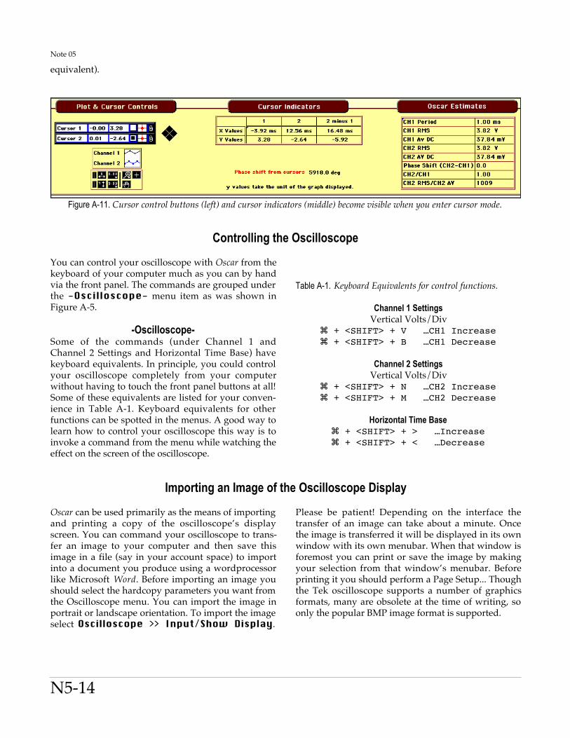
Tek oscilloscopes have cursors to enable you to makespecial measurements of differences in voltage ortime, and Oscar also has cursors. But to activateOscar’s cursors and cursor readouts you first have toenter cursor mode. To enter cursor mode selectCursor >> Enter Cursor Mode (or use thekeyboard equivalent). Only when you do this do thecursor control buttons and cursor indicators becomevisible (middle of Figure A-11).

Cursor ModeIn Oscar, cursors are attached to graphs automaticallyand you can move them up, down, left or right alonga waveform using the triangular blue buttons thatlook like a pointer pad (lower left hand corner of thePanel). To move a cursor place the pointer over theappropriate button and then press and hold down themouse button. As you move a cursor the position of

the cursor is displayed dynamically in the CursorIndicators area. The x and y coordinates of the cursorsare displayed along with differences between the twox-coordinates and the two y-coordinates.

You can also control various attributes of a plot.Plot controls are placed below the cursor controlbuttons. When in cursor mode you can use thesecontrols to change the appearance of the graph or toperform various zoom functions (accessable via themagnifying glass tool). To select a plot control placethe pointer over the control, hold the mouse buttondown and select.

When in cursor mode many of Oscar’s functionsnormally accessable from the main menubar are deac-tivated. To make them active you have to exit cursormode. When you have finished cursoring around andwish to exit cursor mode just select Cursor >> EnterCursor Mode a second time (or use the keyboard

Note 05

N5-14

equivalent).

Figure A-11. Cursor control buttons (left) and cursor indicators (middle) become visible when you enter cursor mode.

Controlling the Oscilloscope

You can control your oscilloscope with Oscar from thekeyboard of your computer much as you can by handvia the front panel. The commands are grouped underthe -Oscilloscope- menu item as was shown inFigure A-5.

-Oscilloscope-Some of the commands (under Channel 1 andChannel 2 Settings and Horizontal Time Base) havekeyboard equivalents. In principle, you could controlyour oscilloscope completely from your computerwithout having to touch the front panel buttons at all!Some of these equivalents are listed for your conven-ience in Table A-1. Keyboard equivalents for otherfunctions can be spotted in the menus. A good way tolearn how to control your oscilloscope this way is toinvoke a command from the menu while watching theeffect on the screen of the oscilloscope.

Table A-1. Keyboard Equivalents for control functions.

Channel 1 SettingsVertical Volts/Div

+ <SHIFT> + V …CH1 Increase + <SHIFT> + B …CH1 Decrease

Channel 2 SettingsVertical Volts/Div

+ <SHIFT> + N …CH2 Increase + <SHIFT> + M …CH2 Decrease

Horizontal Time Base + <SHIFT> + > …Increase + <SHIFT> + < …Decrease

Importing an Image of the Oscilloscope Display

Oscar can be used primarily as the means of importingand printing a copy of the oscilloscope’s displayscreen. You can command your oscilloscope to trans-fer an image to your computer and then save thisimage in a file (say in your account space) to importinto a document you produce using a wordprocessorlike Microsoft Word. Before importing an image youshould select the hardcopy parameters you want fromthe Oscilloscope menu. You can import the image inportrait or landscape orientation. To import the imageselect Oscilloscope >> Input/Show Display.

Please be patient! Depending on the interface thetransfer of an image can take about a minute. Oncethe image is transferred it will be displayed in its ownwindow with its own menubar. When that window isforemost you can print or save the image by makingyour selection from that window’s menubar. Beforeprinting it you should perform a Page Setup... Thoughthe Tek oscilloscope supports a number of graphicsformats, many are obsolete at the time of writing, soonly the popular BMP image format is supported.

Note 05

N5-15

Getting Help

-Graph Help-Arguably Oscar’s functionality is better explained invarious Help windows the program provides than itis in this document. There is one help window foreach graph type. You should read as much as youhave patience for from the “Show Graph Help” selec-tion from under the -Help- menu. As an example,part of a Help screen is reproduced in Figure A-12.

-Show Help-Oscar also provides help on the meaning of controlsand the content of indicators. To invoke this kind ofhelp select Help >> Show Help and move the mousepointer over the item of interest. A small help windowwill then appear with prepared information.

Figure A-12. Oscar’s Help screen for a YT Single Graph.

Note 05

N5-16

Practice Problems