note 9 closed-loop control - college of · pdf filelecture notes of me 475: introduction to...

Lecture Notes of ME 475: Introduction to Mechatronics

Department of Mechanical Engineering, University Of Saskatchewan, 57 Campus Drive, Saskatoon, SK S7N 5A9, Canada

1

Note 9

Closed-Loop Control



2

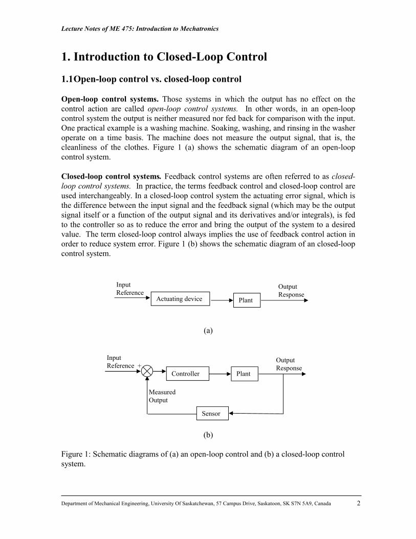
1. Introduction to Closed-Loop Control

1.1 Open-loop control vs. closed-loop control Open-loop control systems. Those systems in which the output has no effect on the control action are called open-loop control systems. In other words, in an open-loop control system the output is neither measured nor fed back for comparison with the input. One practical example is a washing machine. Soaking, washing, and rinsing in the washer operate on a time basis. The machine does not measure the output signal, that is, the cleanliness of the clothes. Figure 1 (a) shows the schematic diagram of an open-loop control system. Closed-loop control systems. Feedback control systems are often referred to as closed-loop control systems. In practice, the terms feedback control and closed-loop control are used interchangeably. In a closed-loop control system the actuating error signal, which is the difference between the input signal and the feedback signal (which may be the output signal itself or a function of the output signal and its derivatives and/or integrals), is fed to the controller so as to reduce the error and bring the output of the system to a desired value. The term closed-loop control always implies the use of feedback control action in order to reduce system error. Figure 1 (b) shows the schematic diagram of an closed-loop control system.

(a)

(b) Figure 1: Schematic diagrams of (a) an open-loop control and (b) a closed-loop control system.

Plant Actuating device

Input Reference

Output Response

Plant

Sensor

Controller

Input Reference

Measured Output

Output Response +

_



3

Closed-loop versus open-loop control systems. An advantage of the closed-loop control system is the fact that the use of feedback makes the system response relatively insensitive to external disturbances and internal variations in system parameters. It is thus possible to use relatively inaccurate and inexpensive components to obtain the accurate control of a given plant, whereas doing so is impossible in the open-loop case. From the stability point of view, the open-loop control system is easier to build because system stability is not a major problem. On the other hand, stability is a major problem in the closed-loop control system, which may tend to overcorrect errors that can cause oscillations of constant or changing amplitude.

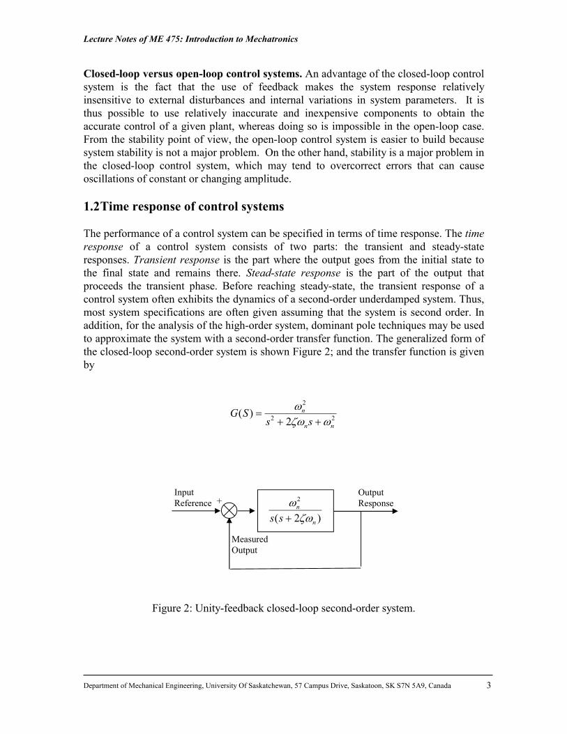
1.2 Time response of control systems The performance of a control system can be specified in terms of time response. The time response of a control system consists of two parts: the transient and steady-state responses. Transient response is the part where the output goes from the initial state to the final state and remains there. Stead-state response is the part of the output that proceeds the transient phase. Before reaching steady-state, the transient response of a control system often exhibits the dynamics of a second-order underdamped system. Thus, most system specifications are often given assuming that the system is second order. In addition, for the analysis of the high-order system, dominant pole techniques may be used to approximate the system with a second-order transfer function. The generalized form of the closed-loop second-order system is shown Figure 2; and the transfer function is given by

22

2

2)(

nn

n

ssSG

Figure 2: Unity-feedback closed-loop second-order system.

)2(

2

n

n

ss

Input Reference

Measured Output

Output Response +

_



4

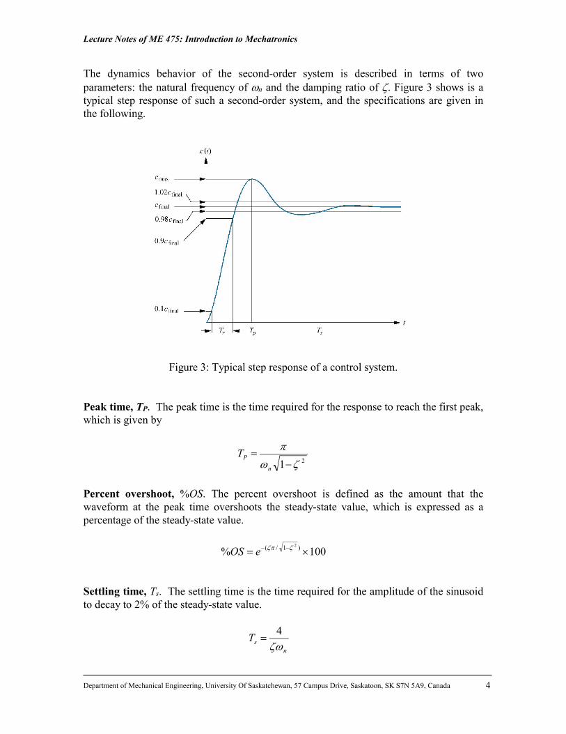
The dynamics behavior of the second-order system is described in terms of two parameters: the natural frequency of n and the damping ratio of . Figure 3 shows is a typical step response of such a second-order system, and the specifications are given in the following.

Figure 3: Typical step response of a control system. Peak time, TP. The peak time is the time required for the response to reach the first peak, which is given by

21

n

PT

Percent overshoot, %OS. The percent overshoot is defined as the amount that the waveform at the peak time overshoots the steady-state value, which is expressed as a percentage of the steady-state value.

100% )1/( 2

eOS Settling time, Ts. The settling time is the time required for the amplitude of the sinusoid to decay to 2% of the steady-state value.

n

sT

4



5

In most control design, the interest is specifically in the final value, or steady-state output value. This is known as steady-state accuracy. Ideally, in the steady-state phase, the system tracks the input reference and the steady-state error is zero. The steady-state error is the difference between the input and the output for a prescribed test input (typically a step) as t . Consider the following feedback system Recall the closed-loop transfer function of the system, T(s), is

)()(1

)(

)(

)()(

sHsG

sG

sR

sCsT

The system output can then be expressed as

)()(1

)()()()()(

sHsG

sGsRsTsRsC

The error, E(s), between the system input, R(s), and the measured output, C(s) H(s), is

)()(1

)()()()()(

sHsG

sRsHsCsRsE

Using the final value theorem, the steady-state error is

)()(1

)(lim)(

0 sHsG

ssRe

s

For a step input, i.e., )()( tutr , its Laplace transform is s

sR1

)( , the steady-state error is

)()(lim1

1

)(1

/1lim)(

0

0 sHsGsG

sse

s

s

.

_

+ E(s) C(s) R(s) G(s)

H(s)



6

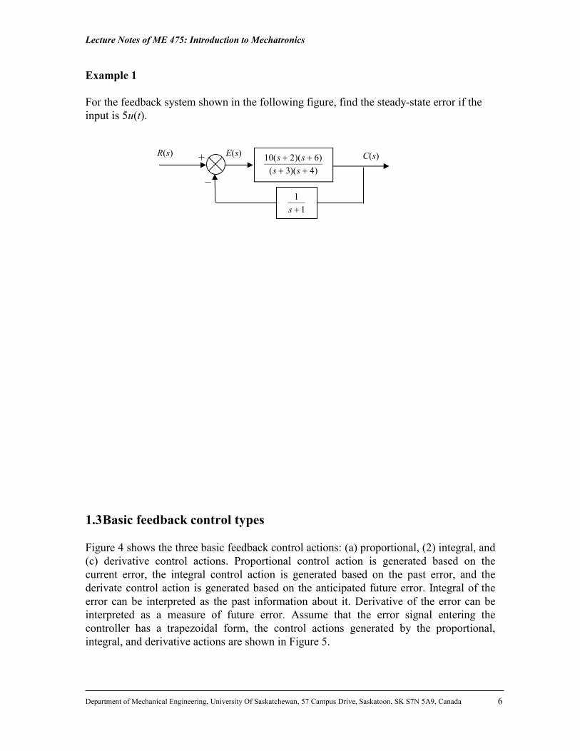
Example 1 For the feedback system shown in the following figure, find the steady-state error if the input is 5u(t).

1.3 Basic feedback control types Figure 4 shows the three basic feedback control actions: (a) proportional, (2) integral, and (c) derivative control actions. Proportional control action is generated based on the current error, the integral control action is generated based on the past error, and the derivate control action is generated based on the anticipated future error. Integral of the error can be interpreted as the past information about it. Derivative of the error can be interpreted as a measure of future error. Assume that the error signal entering the controller has a trapezoidal form, the control actions generated by the proportional, integral, and derivative actions are shown in Figure 5.

C(s)

_

+ E(s) R(s)

)4)(3(

)6)(2(10

ss

ss

1

1

s



7

Figure 4: Basic feedback control actions: proportional, integral, and derivative. Based on the aforementioned three feedback control action, various controllers can be constituted, such as proportional (P) controller, proportional-integral (PI) controller, proportional-derivative (PD) controller, and proportional-integral-derivative (PID) controller, to achieve desired control performance. As an example, Figure 6 shows the block diagram of a PID controller. The control algorithm can be expressed in both continuous (analog) time domain (which can be implemented using op-amps) and in discrete (digital) time domain (which can be implemented using digital computers). At any given time, t, the control signal, u(t) is determined as a function

)()()()(0

teKdeKteKtu D

t

IP

which shows that the control signal is a function of the error between the commanded and measured output signals, e(t) at time t, as well as the derivative of the error signal, )(te ,

and the integral of the error signal since the control loop is enable (t = 0), t

de0

)( .



8

Figure 5: Illustration of the input-output behavior of the basic feedback control actions.

Figure 6: Block diagram of a PID controller.



9

Design of controller via root locus that is introduced in ME 431 is one of the methods that we can use. Design via root locus requires that the designer has the mathematic model of the plant. However, if the plant is complicated, a mathematical model cannot be easily be derived, and analytical approach to the design of a controller is not possible. In such cases, experimental methods need to be used. Ziegler and Nichols developed such a method for tuning the controller parameters based on experiments, called ultimate sensitivity method. In this method, the criteria for adjusting the parameters are based on evaluating the amplitude and frequency of oscillations of the system at the limit of stability. To use the method, the proportional gain is increased until the system becomes marginally stable, as shown in Figure 7. The corresponding gain is defined as Ku (called the ultimate gain) and the period of oscillation is Pu (called the ultimate period). Pu should be measured when the amplitude of oscillation is as same as possible. The tuning parameters are selected as shown in the following Table 1.

Figure 7: Determination of ultimate gain and period.

Table 1: Ziegler-Nichols tuning for the controller

sT

sTKsD D

I

Pc

11)( .

An example of using the ultimate sensitivity method is illustrated in class.

_

+ y(t) r(t) KP Plant



10

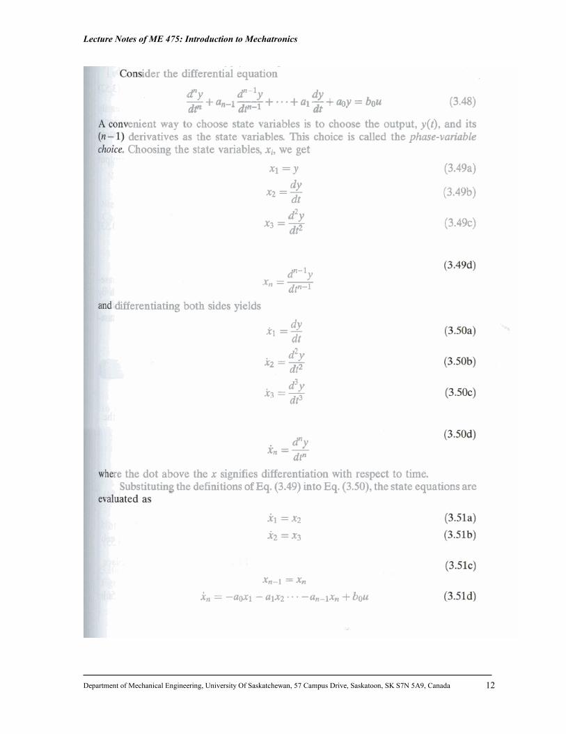
2. Design Via State Space

4.1 State-Space Representation Consider a mechanical system given in the following, with M = 1 kg, K = 100 N/m and fv = 12 N-s/m

Linear combination. A linear combination of n variables, xi, for i = 1 to n, is given by the following sum, S:

1111 xKxKxKS nnnn

Linear independence. A set of variable is said to be linearly independence if none of the variables can be written as a linear combination of the others. System variable. Any variable that responds to an input or initial conditions in a system. State variables. The smallest set of linearly independent system variables. State vector. A vector whose elements are the state variables. State equations. A set of n simultaneous, first-order differential equation with n variables, where the n variables to be solved are the state variables. Output equation. The algebraic equation that expresses the output variables of a system as linear combinations of the state variables and inputs.

y(t)

u(t)



11

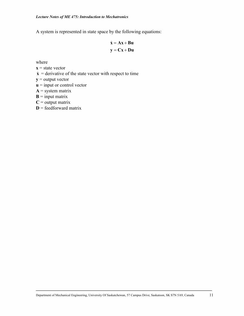
A system is represented in state space by the following equations:

DuCxy

BuAxx

where x = state vector x = derivative of the state vector with respect to time y = output vector u = input or control vector A = system matrix B = input matrix C = output matrix D = feedforward matrix



12



13

Example 2. Find the state-space representation of the transfer function shown in following figure.



14

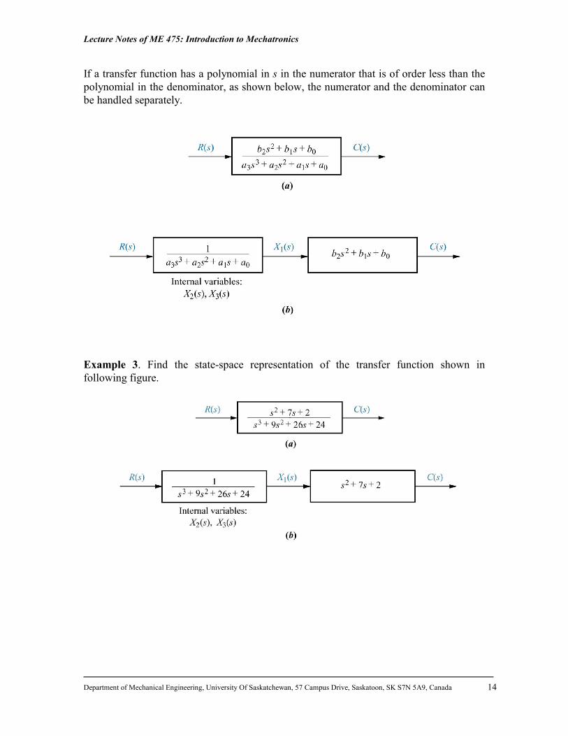
If a transfer function has a polynomial in s in the numerator that is of order less than the polynomial in the denominator, as shown below, the numerator and the denominator can be handled separately.

Example 3. Find the state-space representation of the transfer function shown in following figure.



15

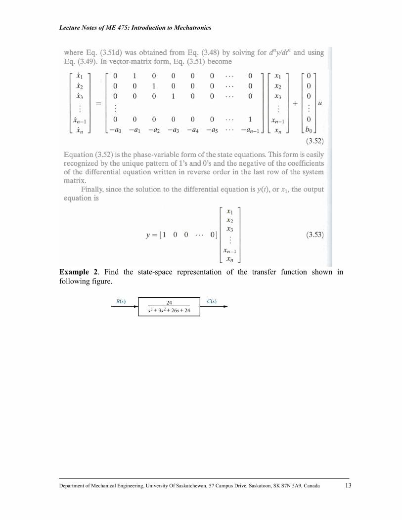
4.2 Control Design Via State-Space This section shows how to introduce additional parameters into a system so that we can control the location of all closed-loop poles. An nth-order feedback control system has a nth-order closed-loop characteristic equation of the form

0011

1 asasas n

nn

Since the coefficient of the highest power of s is unity, there are n coefficients whose values determine the system closed-loop pole locations. Thus, if we can introduce n adjustable parameters into the system and relate them to the coefficients in the above equation, all of the poles of the closed-loop system can be set to any desired location. The idea behind the introduction of n adjustable parameters into the system will be illustrated in class.

(a) State-space representation of a plant (b) Plant with state-variable feedback



16

Design Problem: Given the plant

)4)(1(

)5(20)(

sss

ssG

Design the feedback gains to yield 9.5% overshoot and a settling time of 0.74 second.



17

3. Analog Implementation of Controllers A controller can be realized by op-amps. Figure 8 shows such a circuit in general, and its transfer function is given by

)(

)(

)(

)(

1

2

sZ

sZ

zV

zV

i

o

By judicious choice of Z1(s) and Z2(s), this circuit can be used as a building block to implement the controllers, such as PID controllers. Table 2 summarized the realization of common controllers.

Figure 8: Op-amps for controller realization.

Table 2: Implementation of controllers using op-amps.



18

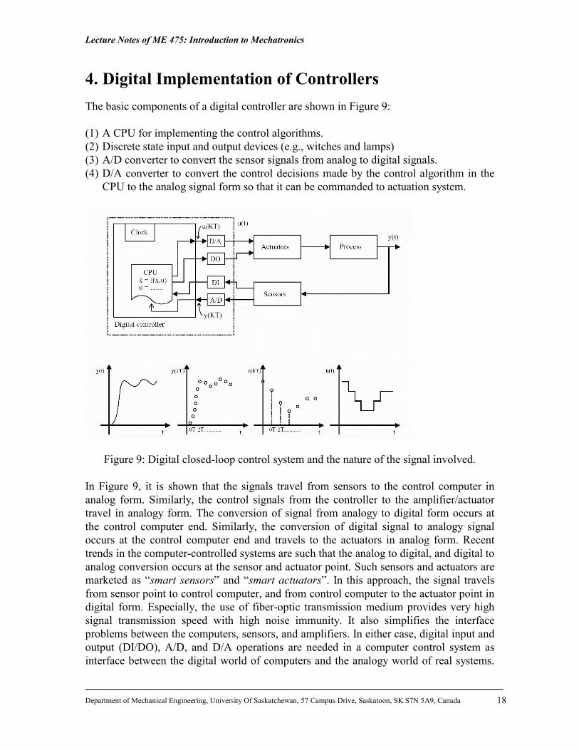
4. Digital Implementation of Controllers

The basic components of a digital controller are shown in Figure 9: (1) A CPU for implementing the control algorithms. (2) Discrete state input and output devices (e.g., witches and lamps) (3) A/D converter to convert the sensor signals from analog to digital signals. (4) D/A converter to convert the control decisions made by the control algorithm in the

CPU to the analog signal form so that it can be commanded to actuation system.

Figure 9: Digital closed-loop control system and the nature of the signal involved.

In Figure 9, it is shown that the signals travel from sensors to the control computer in analog form. Similarly, the control signals from the controller to the amplifier/actuator travel in analogy form. The conversion of signal from analogy to digital form occurs at the control computer end. Similarly, the conversion of digital signal to analogy signal occurs at the control computer end and travels to the actuators in analog form. Recent trends in the computer-controlled systems are such that the analog to digital, and digital to analog conversion occurs at the sensor and actuator point. Such sensors and actuators are marketed as “smart sensors” and “smart actuators”. In this approach, the signal travels from sensor point to control computer, and from control computer to the actuator point in digital form. Especially, the use of fiber-optic transmission medium provides very high signal transmission speed with high noise immunity. It also simplifies the interface problems between the computers, sensors, and amplifiers. In either case, digital input and output (DI/DO), A/D, and D/A operations are needed in a computer control system as interface between the digital world of computers and the analogy world of real systems.



19

The exact location of the digital and analog interface functions may vary from application to application. Digital control systems can be modeled adequately by the discrete equivalent to the differential equation, namely the difference equation. For example, the general second-order difference equation

)2()()()2()()( 012012 TkTxbTkTxbkTxbTkTyaTkTyakTya

where y is the system output and x is the system input. In analog or continuous control systems, we used Laplace transforms in our analysis. In a similar manner, in digital control systems we need to use a new transformation in order to simplify our analysis, which is called the Z-transform. The z-transform is defined by

k

k

zkTfzFKTfz

0

)()()}({

Based on the above definition, we have the equation, called real translation theorem.

)()}({ zFznTKTfz n

Or

)()}({1 nTKTfzFzz n

The Tustin transformation is used to transform the continuous compensator, Gc(s), to the digital compensator, Gc(z). The Tustin transformation is given by

1

12

zT

zs

and its inverse by

sT

sT

z

21

21

As the sampling interval, T, gets smaller (high sampling rate), the digital compensator's output yields a closer match to the analog compensator. If the sampling rate is not high enough, there is a discrepancy at higher frequencies between the digital and analog frequency responses.



20

Example 4 Find the difference equations for the digital implementation of a controller with a transfer

function of s

ssGc

64.1)(

, given that the sampling period is 0.07 s and 0.035 s,

respectively.

note 9 closed-loop control - college of · pdf filelecture notes of me 475: introduction to...

Documents