Noteson

Compressed Sensing

for

Math 394

Simon Foucart

Spring 2009

Foreword

I have started to put these notes together in December 2008. They are intended for agraduate course on Compressed Sensing in the Department of Mathematics at VanderbiltUniversity. I will update them during the Spring semester of 2009 to produce the draftof a coherent manuscript by May 2009. I expect to continue improving it afterwards. Youshould keep in mind that, because Compressed Sensing is a young and rapidly evolvingfield, these notes may become quickly obsolete. Besides, because Compressed Sensing isat the intersection of many scientific disciplines, several lines of approach for a course onthe subject can be taken. The perspective adopted here is definitely a mathematical one,since I am a mathematician by training and by taste. This bias has obviously influencedthe selection of topics I chose to cover, and so has my exposition to the area during thepast few years. Other than reading research articles, this consisted of a Shanks workshopgiven by Joel Tropp at Vanderbilt University, a workshop on the `1-norm held at TexasA&M University, and a series of talks given by Rick Chartrand, Ron DeVore, Anna Gilbert,Justin Romberg, Roman Vershynin, and Mike Wakin at Vanderbilt University.

For a more exhaustive view on Compressed Sensing, the following online resources arerecommended:

• IMA short course on Compressive Sampling and Frontiers in Signal Processing:http://www.ima.umn.edu/2006-2007/ND6.4-15.07/abstracts.html

• Rice Compressed Sensing web site:http://www.compressedsensing.com/

• Igor Carron’s blog, aka Nuit Blanche:http://nuit-blanche.blogspot.com/

I hope that you will enjoy reading these notes. By the end of the course, you will knowalmost as much as I do on the subject, and you should be able to — enthusiastically —conduct research in the area. Any corrections and suggestions are welcome. E-mail me atsimon.foucart@centraliens.net.

Nashville, TN

1

Contents

Foreword 1

Overview 4

1 Motivations and Applications 5

2 Theoretical Limitations 9

3 Reed-Solomon Decoding 17

4 `q-Strategy: Null-Space Property 21

5 `q-Strategy: Stability, Robustness 27

6 A Primer on Convex Optimization 35

7 Coherence and Recovery by `1-minimization 41

8 Restricted Isometry Property and Recovery by `1-Minimization 49

9 Restricted Isometry Property for Random Matrices 54

10 Stable and Robust Recovery with Mixed Norms 67

2

11 Widths 73

12 Using Expander Graphs 82

13 Orthogonal Matching Pursuit 93

14 ROMP and CoSaMP 98

Appendix 1: Some Theorems and Their Proofs 99

Appendix 2: Hints to the Exercises 101

Bibliography 104

3

Overview

...

4

Chapter 1

Motivations and Applications

In Biomedical Imaging, for instance in Magnetic Resonance Imaging, it is not conceivableto collect a number of measurements equal to the number of unknown pixels. Likewise,in wideband radio frequency analysis, limitations in Analog-to-Digital converter technol-ogy prevents the acquisition of a full signal based on Nyquist–Shannon paradigm — seeSection 1.1. However, there is a special feature of images/signals that one can exploit toreconstruct them from such incomplete sets of information: they are compressible, in thesense that they essentially depend on a number of degrees of freedom much smaller thanthe complete information level. Modern transform coders such as JPEG2000 already relyon the fact that images have a sparse — well, almost — representation in a fixed basis. Itis however common to acquire a signal entirely, to compute the complete set of transformcoefficients, to encode the largest ones, and finally to discard all the others. This processis quite wasteful. A digital camera, for instance, uses millions of sensors — the pixels —to finally encode a picture on a few kilobytes. Compressed Sensing offers a way to acquirejust about what is needed, by sampling and compressing simultaneously and by providingefficient decompression algorithms. The ideas of Compressed Sensing are now used on thehardware side to produce new sensing devices, in particular the one-pixel camera is muchtalked about. They are also used in statistical estimation, in studies of cholesterol leveland gene expression, to name but a few, and will probably interface with other fields soon.

1.1 New Sampling Paradigm

A traditional paradigm in Magnetic Imaging Resonance, Astrophysics, and other fieldsof science consists of retrieving a compactly supported function by measuring some of itsfrequency coefficients. This is based on the following theorem — up to duality betweentime and frequency.

5

Theorem 1.1 (Nyquist–Shannon). If the Fourier transform f of a function f satisfiessupp(f) ⊆ [−Ω,Ω], then f is completely determined by its sample values at the pointsnπ/Ω, n ∈ Z, via

f(t) =∞∑

n=−∞f(nπ

Ω

)sinc

(Ω(t− n π

Ω

)).

Now suppose that supp(f) is small, but centered away from the origin, so that Ω is large.The theorem becomes of little value in practice because the different time samples haveto be very close. Compressed Sensing offers the following new paradigm to reconstruct f :sample at m random times t1, . . . , tm, with m of the order of Ω, and reconstruct e.g. byminimizing the `1-norm of the Fourier coefficients subject to the sampling conditions. Theaim of this course is to understand precisely why this works.

1.2 Sparsest Solutions of Underdetermined Linear Systems

In the setting just described, the signal f is expanded as

f =N∑j=1

xjψj ,

for a certain orthonormal basis (ψ1, . . . , ψN ), and such a representation is sparse in thesense that the number s of nonzero xi’s is small compared to N . The signal is then sampledwith a number m of linear measurements, again small compared to N , to obtain the values

(1.1) yi := 〈f, ϕi〉, i ∈ [1 : m].

In the previous setting, we took ϕi as the Dirac distribution δti . The big question is howto choose ϕ1, . . . , ϕm so that the signal f can be reconstructed from the measurementsy1, . . . , ym. Note that knowledge of the signal f and knowledge of the coefficient vector xare equivalent. Thus, we will usually work with x, abusively designating it the signal.The equalities (1.1) translate into the matricial equality y = Ax, where Ai,j = 〈ψj , ϕi〉. Weadopt once and for all the following formulation for our standard problem:

Can we find an m×N sensing matrix A with m N such that any s-sparse vector x ∈ RN

can be recovered from the mere knowledge of the measurement vector y = Ax ∈ Rm?

Of course, since the recovery process only sees the measurements y, two s-sparse vectorsx and x′ satisfying Ax = Ax′ = y must be equal, so that any s-sparse vector x with Ax = y

6

is necessarily the sparsest solution of the underdetermined linear system Az = y. For thisreason, if ‖z‖00 represents the number of nonzero components of the vector z, we may alsoconsider the related problem

(P0) minimize ‖z‖00 subject to Az = y.

We can easily determine a necessary and sufficient condition on the matrix A and thesparsity level s for the standard problem to be solvable. Indeed, writing Σs for the set ofs-sparse vectors in RN , and noticing that Σs − Σs = Σ2s, the condition is

∀x ∈ Σs, ∀x′ ∈ Σs \ x, Ax 6= Ax′, that is ∀u ∈ Σ2s \ 0, Au 6= 0.

In other words, the necessary and sufficient condition is

(1.2) Σ2s ∩ kerA =

0.

However, finding matrices A satisfying this condition is not the end of the story, mainlybecause we do not have a reconstruction procedure available at the moment. Severalprocedures will be introduced in these notes, most notably the `1-minimization recoveryalgorithm. To anticipate slightly, it consists of solving the optimization problem

(P1) minimize ‖z‖1 subject to Az = y.

Here are a few MATLAB commands to illustrate the discussion. The `1-magic software,available online, is required.

>> N=512; m=128; s=25;

>> A=randn(m,N);

>> permN=randperm(N); supp=sort(permN(1:s));

>> x=zeros(N,1); x(supp)=rand(s,1);

>> y=A*x;

>> x1=A\y; xstar=l1eq pd(x1,A,[],y,1e-3);

>> norm(x-xstar)

ans =

2.1218e-05

1.3 Error Correction

Suppose that we encode a plaintext y ∈ Rm by a ciphertext x = By ∈ RN , with N > m. Wethink of the N ×m matrix B as representing a linear code. If B has full rank, then we can

7

decode y from x as

(1.3) y = [B>B]−1B>x.

Now suppose that the ciphertext is corrupted. Thus, we have knowledge of

x = By + e for some error vector e ∈ RN .

It turns out that the plaintext y can still be exactly recovered if B is suitably chosen andif the number s := |i ∈ [1 : N ] : ei 6= 0| of corrupted entries is not too large. Indeed,take N ≥ 2m and consider an m × N matrix A satisfying (1.2) for 2s ≤ m. We thenchoose B as an N ×m matrix that satisfies AB = 0 — pick the m columns of B as linearlyindependent vectors in kerA, which is at least m-dimensional. Because we know the vectorAx = A(By + e) = Ae, Condition (1.2) enable us to recover the error vector e. Finally, theequality By = x− e yields the decoding of the plaintext y as

y = [B>B]−1B>(x− e).

Exercises

Ex.1: Prove the identity (1.3).

Ex.2: Suppose that x ∈ RN is a piecewise constant vector with only a small number s ofjumps, and suppose that we only know the measurement vector y = Ax. It is possibleto recover x by minimizing the `1-norm of a vector z′ depending on a vector z subjectto Az = y. What is this vector z′?

Ex.3: Prove Nyquist–Shannon theorem

Ex.4: Observe that Condition (1.2) implies m ≥ 2s.

Ex.5: Suppose that 2s > m. For 2s×m matrices B, show that plaintexts y ∈ Rm cannot bedecoded from ciphertexts x = By + e with s corrupted entries.

Ex.6: Imitate the MATLAB commands given in Section 1.2 to verify the error correctionprocedure described in Section 1.3.

Ex.7: Suppose that the sparsity is now measured by ‖z‖00,w :=∑

i:zi 6=0wi for some weightsw1, . . . , wN > 0. Find a necessary and sufficient condition in order for each x ∈ RN

with ‖x‖00,w ≤ s to be the unique minimizer of ‖z‖00,w subject to Az = Ax.

8

Chapter 2

Theoretical Limitations

As indicated in Chapter 1, one of the goals of Compressed Sensing is to recover ‘high-dimensional’ signals from the mere knowledge ‘low-dimensional’ measurements. To statesuch a problem in its full generality, we assume that the signals x live in a signal space X,and that they are sampled to produces measurements y = f(x) living in a measurementspace Y . We call the map f : X → Y the measurement map — note that it can alwaysbe assumed to be surjective by reducing Y to f(X). We wish to recover the signal x ∈ X,i.e. we wish to find a reconstruction map g : Y → X such that g(f(x)) = x. Typically, wetake X = RN and Y = Rm with m < N , or better m N , and we choose f as a linearmap. Since a linear map f : RN → Rm cannot be injective, the reconstruction identityg(f(x)) = x cannot be valid for all signals x ∈ RN . Instead, we impose the signals x tobelong to a recoverable class Σ. Typically, the latter class is taken to be the set Σs of alls-sparse vectors, i.e. the set of all vectors with no more than s nonzero components. Notethat Σs can be written as a union of linear subspaces, precisely Σs = ∪|S|≤sΣS , where ΣS isdefined as ΣS := x ∈ RN : xi = 0, i 6∈ S for each index set S ⊆ [1 : N ].

2.1 Minimal Number of Measurements

Given a sparsity level s, we want to know how few measurements are necessary to recovers-sparse vectors. This depends on the signal and measurement spaces X and Y and on thepossible restrictions imposed on the measurement and reconstruction maps f and g. Inothers words, if we translate these restrictions by (f, g) ∈ RX,Y , we want to find

m∗(s;RX,Y ) := infm ∈ N : there exists (f, g) ∈ RX,Y such that g(f(x)) = x, all x ∈ Σs

.

9

We shall distinguish several cases according to the underlying fields of the signal andmeasurement spaces. Namely, we take

X = FN , Y = Km, with F,K ∈Q,R

.

2.1.1 F = R, K = Q, no restriction on f and g

It can be argued that measurements are necessarily rational-valued. In this case, it isimpossible to recover real-valued signals. We have

m∗(s; F = R,K = Q) = +∞.

Indeed, if a suitable m existed, then the reconstruction identity would imply that the mapf|Σs

: Σs → Qm is injective, and in turns that Σs is countable. But this is not so, since Σs

contains all the real lines Σi, i ∈ [1 : N ].

We recall here that a set S is called countable if

(2.1) there exists an injection from S to N,

or equivalently if

(2.2) there exists a surjection from N to S.

2.1.2 F = Q, K = Q, no restriction on f and g

If both measurements and signals are rational-valued, then it is possible to recover anysignal from one single measurement as long as we can freely select the measurement andreconstruction maps. In short,

m∗(s; F = Q,K = Q) = 1.

Indeed, because QN is countable, there exists a surjection g : Q → QN . Thus, for allx ∈ QN , we can choose y =: f(x) ∈ Q such that g(y) = x. With such measurement andreconstruction maps f and g, we have g(f(x)) = x for all x ∈ QN , not just for all x ∈ Σs.

2.1.3 F = R, K = R, no restriction on f and g

For real-valued signals and measurements, it also happens that one single measurementis enough to ensure recovery of all x ∈ QN , not just of all x ∈ Σs, so long as we can freely

10

select the measurement and reconstruction maps. In short,

m∗(s; F = R,K = R) = 1.

Indeed, classical space-filling maps provide surjections g : R → RN , and we constructmeasurement maps f : RN → R just as before.

2.1.4 F = R, K = R, f continuous and antipodal

For real-valued signals and measurements, we shall now impose the measurement mapf : RN → Rm to be continuous and to be antipodal, that is to satisfy f(−x) = −f(x)for all x ∈ RN . For example, a linear map RN → Rm meets these requirements. Theminimal number of measurements necessary to recover sparse vectors is in this case twicethe sparsity. In other words,

m∗(s; F = R,K = R, f continuous and antipodal) = 2s.

For the first part of the proof — that is the inequalitym∗ ≥ 2s— we shall use Borsuk–Ulamtheorem. A proof can be found in Appendix 2.

Theorem 2.1 (Borsuk–Ulam). A continuous antipodal map F : Sn → Rn from the sphereSn of Rn+1 — relative to any norm — into Rn vanishes at least once, i.e. there is a pointx ∈ Sn for which F (x) = 0.

Given m < 2s, let us now assume that it is possible to find a continuous antipodal mapf : RN → Rm which is injective on Σs. Then, taking U := Σ[1:s] and V := Σ[s+1:2s], we definethe continuous antipodal map

F : (u,v) ∈ U × V 7→ f(u)− f(v) ∈ Rm.

Since dim(U × V ) = 2s > m, we can apply Borsuk–Ulam theorem to obtain u ∈ U andv ∈ V with ‖u‖1 + ‖v‖1 = 1 such that F (u,v) = 0. This means that f(u) = f(v). Theinjectivity of f on Σs then implies that u = v. But this yields u = v = 0, which contradicts‖u‖1 + ‖v‖1 = 1. At this point, we have established the inequality

m∗(s; F = R,K = R, f continuous and antipodal) ≥ 2s.

The reverse inequality is established in the next section. As it turns out, we will considerlinear measurement maps to recover s-sparse vectors from 2s measurements.

11

2.2 Totally Positive Matrices

Definition 2.2. A square matrix M is called totally positive, resp. totally nonnegative, if

det(MI,J) > 0, resp. det(MI,J) ≥ 0,

for all index sets I and J of same cardinality. Here MI,J represents the submatrix of Mformed by keeping the rows indexed by I and the columns indexed by J .

Let us now suppose that m = 2s. We consider an N × N totally positive matrix M , fromwhich we extract m rows indexed by a set I to form an m×N submatrix A. For each indexset J of cardinality m = 2s, the submatrix AJ := MI,J is invertible. Therefore, for anynonzero 2s-sparse vector u ∈ RN , say with supp(u) ⊆ J , |J | = 2s, we have Au = AJuJ 6= 0.This establishes Condition (1.2) that Σ2s ∩ kerA = 0. Thus, the linear — in particular,continuous and antipodal — measurement map defined by f(x) = Ax allows reconstructionof every s-sparse vector from m = 2s measurements. This means that

m∗(s; F = R,K = R, f continuous and antipodal) ≤ 2s.

This completes our proof, so long as we can exhibit a totally positive matrix M . We takethe classical example of a Vandermonde matrix.

Proposition 2.3. Given xn > · · · > x1 > x0 > 0, the Vandermonde matrix V :=[xji]ni,j=0

istotally positive.

Proof. We start by proving Descartes’ rule of sign, namely for all (a0, . . . , an) ∈ Rn+1 \ 0,one has

Z(0,∞)(p) ≤ S−(a0, . . . , an), p(x) :=n∑k=0

akxk,

where Z(0,∞)(p) represents the number of zeros of the polynomial p in the interval (0,∞)and where S−(a0, . . . , an) represents the number |i ∈ [1 : n] : ai−1ai < 0| of strong signchanges for the sequence (a0, . . . , an). We proceed by induction on n ≥ 0. For n = 0, therequired result is obvious — it reads 0 ≤ 0. Let us now assume that the required resultholds up to an integer n−1, n ≥ 1. We want to establish that, given (a0, . . . , an) ∈ Rn+1 \0and p(x) :=

∑nk=0 akx

k, we have Z(0,∞)(p) ≤ S−(a0, . . . , an). Note that we may supposea0 6= 0, otherwise the result would be clear from the induction hypothesis, in view of

S−(a0, . . . , an) = S−(a1, . . . , an) ≥ Z(0,∞)

( n−1∑k=0

ak+1xk)

= Z(0,∞)

( n−1∑k=0

ak+1xk+1)

= Z(0,∞)(p).

12

Now let ` be the smallest index in [1 : n] such that a` 6= 0 — if no such index exists, then theresult is clear. Up to the change p↔ −p, there are two cases to consider: [a0 > 0, a` < 0] or[a0 > 0, a` > 0].1/ [a0 > 0, a` < 0]. Applying Rolle’s theorem and the induction hypothesis, we obtain

S−(a0, . . . , an) = S−(a1, . . . , an) + 1 ≥ Z(0,∞)(p′) + 1 ≥ Z(0,∞)(p),

which is the required result.2/ [a0 > 0, a` > 0]. Let t be the smallest positive zero of p — again, if no such t exists,then the result is clear. Suppose that p′ does not vanish on (0, t). This implies that p′ hasa constant sign on (0, t). Since p′(x) =

∑nk=` akkx

k−1, there holds p′(x) > 0 on a certainright neighborhood of 0. Thus we obtain p′(x) > 0 for all x ∈ (0, t), and consequently0 = p(t) > p(0) = a0, which is not the case. Therefore, there is a zero of p′ in (0, t).Taking into account the zeros of p′ guaranteed by Rolle’s theorem, and using the inductionhypothesis, we obtain

S−(a0, . . . , an) = S−(a1, . . . , an) ≥ Z(0,∞)(p′) ≥ Z(0,∞)(p),

which is the required result.The inductive proof of Descartes’ rule of sign is now complete. Next, we shall prove that,for all 0 < x0 < x1 < · · · < xn, 1 ≤ i1 ≤ · · · ≤ i` ≤ n, 1 ≤ j1 ≤ · · · ≤ j` ≤ n, and 1 ≤ ` ≤ n, onehas ∣∣∣∣∣∣∣∣∣∣

xj1i1 . . . xj`−1

i1xj`i1

... . . ....

...xj1i`−1

. . . xj`−1

i`−1xj`i`−1

xj1i` . . . xj`−1

i`xj`i`

∣∣∣∣∣∣∣∣∣∣> 0.

We proceed by induction on ` ∈ [1 : n]. For ` = 1, the required result is nothing else thanthe positivity of all the xi’s. Let us now assume that the required result holds up to aninteger `− 1, ` ≥ 2. Suppose that the required result fails for `, i.e. that

(2.3)

∣∣∣∣∣∣∣∣∣∣xj1i1 . . . x

j`−1

i1xj`i1

... . . ....

...xj1i`−1

. . . xj`−1

i`−1xj`i`−1

xj1i` . . . xj`−1

i`xj`i`

∣∣∣∣∣∣∣∣∣∣≤ 0

for some 0 < x0 < x1 < · · · < xn, 1 ≤ i1 ≤ · · · ≤ i` ≤ n, 1 ≤ j1 ≤ · · · ≤ j` ≤ n, and 1 ≤ ` ≤ n.

13

Let us introduce the polynomial

p(x) :=

∣∣∣∣∣∣∣∣∣∣xj1i1 . . . x

j`−1

i1xj`i1

... . . ....

...xj1i`−1

. . . xj`−1

i`−1xj`i`−1

xj1 . . . xj`−1 xj`

∣∣∣∣∣∣∣∣∣∣.

Expanding with respect to the last row and invoking Descartes’ rules of sign, we getZ(0,∞)(p) ≤ ` − 1. But the polynomial p vanishes at the positive points xi1 , . . . , xi`−1

, hencevanishes only at these points in (0,∞). In view of (2.3), we derive that p(x) < 0 for allx > xi`−1

. But this is absurd because, using the induction hypothesis, we have

limx→∞

p(x)xj`

=

∣∣∣∣∣∣∣∣xj1i1 . . . x

j`−1

i1... . . .

...xj1i`−1

. . . xj`−1

i`−1

∣∣∣∣∣∣∣∣ > 0.

We deduce that the required result holds for `. This concludes the inductive proof.

There is an interesting characterization of totally nonnegative matrices that we mentionhere without justification. By a weighted planar network G of order n, we mean an acyclicplanar directed graph where 2n boundary vertices are distinguished as n sources s1, . . . , sn

and n sinks t1, . . . , tn and where each edge e is assigned a weight w(e) > 0. The path matrixW of the weighted planar network G is defined by

Wi,j :=∑

p path from si to tj

w(p) :=∑

p path from si to tj

∏e edge in p

w(e).

The next lemma provides a simple interpretation for the determinant of W .

Lemma 2.4 (Lindstrom). The determinant of the path matrix W of a weighted planar net-work G equals the weighted number of families of nonintersecting paths from the sourcesto the sinks, i.e.

det(W ) =∑

p1,...,pn non intersecting paths, pi path si→ti

w(p1) · · ·w(pn) ≥ 0.

One can verify from Figure 2.1 that the 3× 3 Vandermonde determinant is given by

det[xji]3i,j=1

= (x2 − x1)(x2 − x0)(x1 − x0).

We can apply Lindstrom’s lemma to any submatrix GI,J of the path matrix G. We wouldobtain the first part of the next theorem. It is quite interesting that the converse also holds.

14

Figure 2.1: The weighted planar network for the 3× 3 Vandermonde matrix

Theorem 2.5. The path matrix of any weighted planar network is totally nonnegative.Conversely, every totally nonnegative matrix is the path matrix of some weighted planarnetwork.

Exercises

Ex.1: Check that (2.1) and (2.2) are indeed equivalent. Using (2.1) or (2.2), establish thatQm is countable and that R is not countable.

Ex.2: Give an example of a plane filling-map R→ R2.

Ex.3: Prove that m∗(s; F = R,K = R, f continuous) ≥ s. Can you do better?

Ex.4: Suppose that Borsuk–Ulam theorem holds relative to some particular norm. Showthat it consequently holds relative to any norm.

Ex.5: Check that the stated formulation of Borsuk–Ulam theorem is equivalent to thefollowing formulation:Theorem. A continuous map G : Sn → Rn from the sphere Sn of Rn+1 into Rn

sends two antipodal points to the same point, i.e. there exists x ∈ Sn for whichG(−x) = G(x).

Ex.6: Prove that the product of two totally positive matrices is a totally positive matrix.

15

Ex.7: Let 0 < x0 < · · · < xn < 1. Use the total positivity of the Vandermonde matrix toestablish that the collocation determinant

det[Bni (xj)

]ni,j=1

, Bni (x) :=

(n

i

)xi(1− x)n−i,

of the Bernstein polynomials Bn0 , . . . , B

nn at the points x0, . . . , xn is totally positive.

Ex.8: Recall the necessary and sufficient condition for an n × n invertible matrix M toadmit a Doolittle’s factorization, i.e. an LU -factorization with ones on the diagonalof L. Observe that any totally positive matrix admits a Doolittle’s factorization. UseNewton’s form of the polynomial interpolant to exhibit the Doolittle’s factorization ofthe transpose of the Vandermonde matrix.

Ex.9: Try to imitate the MATLAB commands of Section 1.2 when A is the matrix formedby m rows of an N ×N Vandermonde matrix.

16

Chapter 3

Reed-Solomon Decoding

We have seen that, if the m×N matrix A is obtained from an N ×N totally positive matrixby selecting m of its rows, then the measurement map defined by f(x) = Ax, x ∈ RN ,allows to reconstruct every s-sparse vector with only m = 2s measurements. In this case,the reconstruction map is given by

g(y) ∈ argmin‖z‖00 : Az = y

.

To find g(y) in a straightforward way, it is required to perform a combinatorial searchwhere all

(Ns

)overdetermined linear systems ASzS = y, |S| = s, have to be solved. This

is not feasible in practice. In this chapter, we shall introduce a practical reconstructionprocedure that seems to do the job with only m = 2s measurements. This procedure,however, has important faults that we shall expose.

3.1 The reconstruction procedure

Let x be an s-sparse vector. In fact, we consider x as a function x defined on [0 : N − 1] withsupp(x) ⊆ S, |S| = s. We shall measure only its first 2s discrete Fourier coefficients, namely

x(j) :=N−1∑k=0

x(k)e−i2πjk/N , j ∈ [0 : 2s− 1].

We then consider the trigonometric polynomial of degree s defined by

p(t) :=∏k∈S

(1− e−i2πk/Nei2πt/N ),

17

which vanishes exactly for t ∈ S. In view of 0 = p(t) · x(t), t ∈ [0, N − 1], we obtain bydiscrete convolution

(3.1) 0 = (p ∗ x)(j) =N−1∑k=0

p(k) · x(j − k), j ∈ [0 : N − 1].

We take into account that the coefficient p(k) of the trigonometric polynomial p(t) on themonomial ei2πkt/N vanishes for k > s and that its coefficient p(0) on the constant monomial1 equals 1 to rewrite the equations of (3.1) corresponding to j ∈ [s : 2s− 1] as

x(s) + p(1) · x(s− 1) + · · · + p(s) · x(0) = 0,x(s+ 1) + p(1) · x(s) + · · · + p(s) · x(1) = 0,

...... · · ·

......

x(2s− 1) + p(1) · x(2s− 2) + · · · + p(s) · x(s− 1) = 0.

This translates into the Toeplitz system 1x(s− 1) x(s− 2) · · · x(0)x(s) x(s− 1) · · · x(1)

... . . . ...x(2s− 2) x(2s− 3) · · · x(s− 1)

p(1)p(2)

...p(s)

= −

x(s)

x(s+ 1)...

x(2s− 1)

.

Because x(0), . . . , x(2s − 1) are known, we can solve for p(1), . . . , p(s). This determines pcompletely. In turns, the trigonometric polynomial p is completely determined by takingthe inverse discrete Fourier transform. Then we just need to find the zeros of p to obtainthe support of x. Once this is done, we can deduce x exactly by solving an overdeterminedsystem of linear equations.

3.2 Implementation

We recall right away that the process of finding the roots of a polynomial — trigonometricor algebraic — is highly unstable. Therefore, instead of solving p(t) = 0 to find the supportof x, we will simply select the indices j yielding the s smallest values for |p(j)|. Here arethe MATLAB commands to test the Reed-Solomon decoding we have just described.

>> N=500; s=18;

>> supp=sort(randsample(N,s));

1the Toeplitz matrix is not always invertible: take e.g. x = [1, 0, . . . , 0]>, so that x = [1, 1, . . . , 1]>,

18

>> x=zeros(N,1); x(supp)=randn(s,1);

>> xhat=fft(x); y=xhat(1:2*s);

>> phat=zeros(N,1); phat(1)=1;

>> A=toeplitz(y(s:2*s-1),y(s:-1:1));

>> phat(2:s+1)=-A\y(s+1:2*s);>> p=ifft(phat);

>> [sorted p,ind]=sort(abs(p)); rec supp=sort(ind(1:s));

>> [supp’;rec supp’]

ans =

17 43 45 48 73 90 91 141 154 253 255 307 321 344 439 456 486 492

17 43 45 48 73 90 91 141 154 253 255 307 321 344 439 456 486 492

3.3 Non-robustness

In practice, we cannot measure the discrete Fourier coefficients with infinite precision, soour 2s measurement are in fact a slight perturbation of x(0), . . . , x(2s−1). It turns out thatthis small inaccuracy causes the procedure to badly misbehave. The following numericalexperiment illustrates this point.

>> N=500; s=18;

>> supp=sort(randsample(N,s));

>> x=zeros(N,1); x(supp)=randn(s,1);

>> xhat=fft(x); noise=randn(2*s,1)/10ˆ4; y=xhat(1:2*s)+noise;

>> phat=zeros(N,1); phat(1)=1;

>> A=toeplitz(y(s:2*s-1),y(s:-1:1));

>> phat(2:s+1)=-A\y(s+1:2*s);>> p=ifft(phat);

>> [sorted p,ind]=sort(abs(p)); rec supp=sort(ind(1:s));

>> [supp’;rec supp’]

ans =

8 23 91 167 177 212 214 220 248 266 284 338 354 410 424 433 489 491

8 9 23 91 167 177 212 248 266 284 338 354 410 424 433 487 488 489

19

Exercises

Ex.1: A circulant matrix is a particular Toeplitz matrix of the form

c0 c1 c2 · · · cN−1

cN−1 c0 c1 · · · cN−2

cN−2 cN−1 c0. . . ...

... . . . . . . c1

c1 c2 · · · cN−1 c0

.

Under which conditions is a circulant matrix invertible? Calculate the determinantof such a matrix using its eigenstructure.

Ex.2: Find the determinant of the Toeplitz matrix

a b b · · · b

c a b · · · b

c c a. . . ...

...... . . . . . . b

c c · · · c a

.

Ex.3: Prove that the discrete Fourier transform converts product into discrete convolution,and vice versa.

Ex.4: This classical example illustrates the instability of root finding. We consider theWilkinson polynomial p(x) = (x− 1)(x− 2) · · · (x− 20). Alter this polynomial slightlyto form p(x)+10−8x19, and investigate numerically what happens to the largest roots.

Ex.5: This exercise illustrates the non-stability of Reed–Solomon decoding. Assume that xis not an s-sparse vector, but is close to one. Apply the Reed–Solomon procedure anddetermine if the result is close to the original vector x.

20

Chapter 4

`q-Strategy: Null-Space Property

The sparsity ‖z‖00 of a given vector z ∈ RN can be approximated by the q-th power of its`q-quasinorm when q > 0 is small. The observation that

‖z‖qq :=N∑j=1

|zj |q −→q→0

N∑j=1

1zj 6=0 = ‖z‖00, z ∈ RN ,

is the premise of this chapter. It suggests substituting the problem (P0) by the problem

(Pq) minimize ‖z‖qq subject to Az = y.

4.1 Null-Space Properties

We need to highlight the following fact as a prerequisite to our analysis.

Lemma 4.1. For 0 < q ≤ 1, the q-th power of the `q-quasinorm induces a metric on RN

defined by d(u,v) := ‖u− v‖qq for u,v ∈ RN

Proof. That d(u,v) = d(v,u) and that [d(u,v) = 0] ⇐⇒ [u = v] are clear. To establishthe triangle inequality d(u,w) ≤ d(u,v) + d(v,w) for u,v,w ∈ R, it is enough to show that‖a + b‖qq ≤ ‖a‖qq + ‖b‖qq for a,b ∈ RN . Working component by component, it suffices toprove that (α+ β)q ≤ αq + βq whenever α, β ≥ 0. If α = 0, then this is obvious. If otherwiseα > 0, then we need to show that (1 + γ)q ≤ 1 + γq for γ := β/α ≥ 0. Simply observe thatthe function h defined by h(γ) := (1 + γ)q − 1− γq is negative on (0,∞), since h(0) = 0 andh′(γ) = q[(1 + γ)q−1 − γq−1] < 0 for γ > 0.

Let us point out that the assumption m ≥ 2s is made throughout this chapter — andimplicitly in the rest of these notes. Recall that it is in any case necessary for the exact

21

reconstruction of s-sparse vectors x ∈ RN from the measurements y = Ax ∈ Rm. Let usnow suppose that, given any s-sparse vector x ∈ RN , solving the problem (Pq) with y = Axreturns the vector x as unique output. Then, for a vector v ∈ kerA \ 0 and an indexset S ⊆ [1 : N ] with |S| ≤ s, we have A(−vS) = AvS . Since the vector vS is s-sparse anddifferent from the vector −vS , we must have ‖vS‖qq < ‖vS‖

qq. Conversely, let us suppose

that ‖vS‖qq < ‖vS‖qq for all v ∈ kerA \ 0 and all S ⊆ [1 : N ] with |S| ≤ s. Then, given

an s-sparse vector x ∈ RN and a different vector z ∈ RN satisfying Az = Ax, we havev := x− z ∈ kerA \ 0. Specifying S = supp(x), we get

‖x‖qq ≤ ‖x− zS‖qq + ‖zS‖qq = ‖vS‖qq + ‖zS‖qq < ‖vS‖qq + ‖zS‖qq = ‖ − zS‖qq + ‖zS‖qq = ‖z‖qq.

Thus, the s-sparse vector x is the unique solution of (Pq) with y = Ax. At this point,we have established a necessary and sufficient condition for exact recovery of all s-sparsevectors by `q-minimization. This condition on the matrix A and the sparsity s is called theNull-Space Property relative to `q. It reads

(NSPq) ∀v ∈ kerA \ 0, ∀ |S| ≤ s, ‖vS‖qq < ‖vS‖qq.

By adding ‖vS‖qq to both sides of the inequality and rearranging the terms, we can alsostate the Null-Space Property in the form

∀v ∈ kerA \ 0, ∀ |S| ≤ s, ‖vS‖qq < 12‖v‖

qq.

Let us briefly mention two properties that a reasonable reconstruction scheme shouldposses: if we add some measurements, then the recovery should be preserved, and if weamplify some measurements, then the recovery should also be preserved. Mathematically

speaking, this translates into replacing the m×N matrix A by an m′×N matrix A :=

[A

B

]for an (m′ − m) × N matrix B, or by an m × N matrix A = DA for a nonsingular m × mdiagonal matrix D. In these two cases, `q-recovery is preserved, because the correspondingNull-Space Properties remain fulfilled, in view of ker A ⊆ kerA and ker A = kerA.

4.2 Reconstruction exponents

It is natural to enquire about the success of `q-recovery as a function of the exponent q.The main result of this section is the justification of the intuitive belief that `q-recoveryshould imply `r-recovery for all r < q. Before establishing this, let us start with the simpleobservation that `q-recovery is impossible if q > 1.

22

Lemma 4.2. If q > 1, then for any m × N matrix A with m < N , there exists a 1-sparsevector which is not recovered by `q-minimization.

Proof. Let us consider an exponent q > 1. For j ∈ [1 : N ], let ej ∈ RN be the 1-sparse vectorwhose j-th component equals one. Now suppose that, for all z ∈ RN satisfying Az = Aejand z 6= ej , we have ‖z‖qq > ‖ej‖qq = 1. Considering a vector v ∈ kerA \ 0 and a realnumber t 6= 0 with |t| < 1/‖v‖∞, we obtain

1 < ‖ej + tv‖qq = |1 + t vj |q +N∑

k=1, k 6=j|t vk|q = (1 + t vj)q + tq

N∑k=1, k 6=j

|vk|q ∼t→0

1 + q t vj .

For this to happen, we need vj = 0. The fact that this should be true for all j ∈ [1 : N ] isclearly in contradiction with v 6= 0.

The next observation concerns the set Qs(A) of reconstruction exponents, that is the set ofall exponents 0 < q ≤ 1 for which every s-sparse vector x ∈ RN is recovered as the uniquesolution of (Pq) with y = Ax. Although we will not use the following observation, let usnotice that, according to the Null-Space Property relative to `q, the set of reconstructionexponents can be written as

Qs(A) :=q ∈ (0, 1] : ∀ |S| ≤ s, ‖RA,S‖q < (1/2)1/q

,

where for an index set S ⊆ [1 : N ], the notation RA,S denotes the restriction operatorfrom kerA into RN as defined by RA,S(v) := vS , v ∈ kerA, and where the expression‖RA,S‖q := sup

‖RA,S(v)‖q, ‖v‖q = 1

represents the `q-quasinorm of the operator RA,S

Proposition 4.3. The setQs(A) of reconstruction exponents is a — possibly empty — openinterval

(0, q∗(A)

). The right endpoint q∗s(A) ∈ [0, 1] is called the critical reconstruction

exponent of the matrix A with respect to the sparsity s.

Proof. Let us remark that to establish the Null-Space Property for a given v ∈ kerA \ 0,it is enough to consider the index set S of the s largest absolute-value components of v.Note then that the condition ‖vS‖qq < ‖vS‖

qq can be rewritten as

(4.1)∑j∈S

|vj |q∑k∈S |vk|q

< 1.

Now, given an index j ∈ S, the quantity

|vj |q∑k∈S |vk|q

=1∑

k∈S(|vk|/|vj |

)q23

is an increasing function of q ∈ (0, 1], since |vk|/|vj | ≤ 1 for k ∈ S. Thus, summing overj ∈ S, we see that the inequality (4.1) is fulfilled for all r ∈ (0, q) as soon as it if fulfilledfor a certain q ∈ (0, 1]. This shows that Qs(A) is an interval of the type

(0, q∗(A)

)or of the

type(0, q∗(A)

]. Let us prove that it is of the former type. For this purpose, let us consider

a sequence (qn) of exponents in Qs(A) converging to q := q∗s(A) ∈ (0, 1]. For each integer n,there exists an index set Sn ⊆ [1 : N ] with |Sn| ≤ s and a vector vn ∈ kerA with ‖vn‖qnqn = 1and ‖vn,Sn‖

qnqn ≥ 1/2. Note that we can extract a constant subsequence (Snk

) =: (S) out ofthe sequence (Sn), since there is only a finite number of subsets of cardinality s in [1 : N ].Then, because the sequence (vnk

) has values in the unit ball of the finite-dimensional spacekerA endowed with the `∞-norm, we can extract a subsequence that converges to somev ∈ kerA. The equality ‖vnk

‖qnkqnk

= 1 and the inequality ‖vnk,S‖qnkqnk≥ 1/2 pass to the limit to

give ‖v‖qq = 1 and ‖vS‖qq ≥ 1/2. Thus, the Null-Space Property relative to `q is not satisfied.This proves that q = q∗s(A) ∈ Qs(A), as required.

4.3 Reconstruction and sign pattern of sparse vectors

Although we were varying the index set S in the previous sections, most of our analysisremains valid if the index set S is fixed. For such a context, we present in this sectiona result reminiscent of the Null-Space Property. It has an interesting corollary, whichroughly states that `1-minimization succeeds in recovering vectors supported exactly on S

only according to their sign patterns. But beware, recovering x by `1-minimization meanshere that x is a minimizer of ‖z‖1 subject to Az = Ax, not necessarily the unique minimizer.

Proposition 4.4. Given an index set S ⊆ [1 : N ], and given a vector x ∈ RN whose supportis exactly S, one has

[∀ z ∈ RN with Az = Ax, ‖z‖1 ≥ ‖x‖1] ⇐⇒ [∀v ∈ kerA,∑j∈S

sgn(xj)vj ≤ ‖vS‖1].

Proof. The left-hand side condition is equivalent to

∀v ∈ kerA, ‖x− v‖1 ≥ ‖x‖1.

The desired result will follow from a characterization of best approximation in `1-norm.We refer to the Appendix for a characterization of best approximation in a general normedspace. Using this result and the fact that

Ex(B∗`N1

) ∼= Ex(B`N∞) =ε ∈ RN : ∀ j ∈ [1 : N ], εj = ±1

,

24

the characterization takes the form

∀v ∈ kerA, ∃ ε1, . . . , εN = ±1 :N∑j=1

εj(xj − vj) ≥N∑j=1

εjxj =N∑j=1

|xj |.

The latter equality implies that εj = sgn(xj) on supp(x) = S. Simplifying, we obtain theequivalent condition

∀v ∈ kerA, ∃ (ηj)j∈S ∈ −1, 1S :∑j∈S

sgn(xj)vj ≤∑j∈S

ηjvj .

Finally, this turns out to be equivalent to the condition

∀v ∈ kerA,∑j∈S

sgn(xj)vj ≤ ‖vS‖1,

as expected.

4.4 Mixed-Norm Null-Space Properties

Typically, it is difficult to work directly with the `q-quasinorm, hence it is often preferableto obtain first estimates for the Euclidean `2-norm, and then to derive estimates for the`q-quasinorm. This step involves the following classical inequalities.

Lemma 4.5. Given 0 < q < p ≤ ∞, there holds

‖x‖p ≤ ‖x‖q ≤ n1/q−1/p‖x‖p, x ∈ Rn,

and these inequalities are sharp.

Proof. Consider first of all the vectors x = [1, 0, . . . , 0]> and x = [1, 1, . . . , 1]> to observe thatthe constants 1 and n1/q−1/p in the inequalities ‖x‖p ≤ 1 · ‖x‖q and ‖x‖q ≤ n1/q−1/p · ‖x‖pcannot be improved. Next, to establish the first inequality, we observe that it is sufficientto prove it for ‖x‖q = 1, by homogeneity. In this case, we have |xi| ≤ 1 for all i ∈ [1 : n],so that |xi|p ≤ |xi|q. Summing over all i’s yields ‖x‖pp ≤ 1, i.e. ‖x‖p ≤ 1, which is what wewanted. Finally, to establish the second inequality, we simply use Holder’s inequality towrite

‖x‖qq =n∑i=1

1 · |xi|q ≤[ n∑i=1

1r]1/r·[ n∑i=1

(|xi|q

)p/q]q/p = n1/r · ‖x‖qp,

where r satisfies 1/r + q/p = 1, i.e. 1/r = 1 − q/p. Taking the q-th root, we obtain therequired inequality.

25

Given 0 < q ≤ 1 and p ≥ q, the previous lemma implies that ‖vS‖q ≤ s1/q−1/p · ‖vS‖p for alls-sparse vectors v ∈ RN . Therefore, the following conditions, which we call `p-Strong Null-Space Properties relative to `q, are enough to guarantee exact reconstruction of s-sparsevectors x ∈ RN from the measurements y = Ax ∈ Rm by `q-minimization. They read

(NSPp, q) ∀v ∈ kerA, ∀ |S| ≤ s, ‖vS‖q <

1

s1/q−1/p‖vS‖q,

(1/2)1/q

s1/q−1/p‖v‖q.

Exercises

Ex.1: A quasinorm · on a vector space X is a function from X into [0,∞) for whichthere exists a constant c > 0 such that λx = |λ| x, x + y ≤ c

( x + y

),

and [x = 0] ⇒ [x = 0]. Prove that the expressions ‖x‖q =∑n

i=1 |xi|q, x ∈ Rn, and‖T‖q = sup

‖Tx‖q, ‖x‖q = 1

, T ∈ Rn×n, indeed define quasinorms. Note that a

quasinorm is different from a seminorm · : X → [0,∞), also called pseudonorm,which satisfies λx = |λ|x and x+y ≤ x+y, but not [x = 0]⇒ [x = 0].

Ex.2: Make sure that the Null-Space Property implies the condition Σ2s ∩ kerA = 0.

Ex.3: Fixing a sparsity s, find a matrix whose critical reconstruction exponent is equal toa prescribed q ∈ (0, 1].

Ex.4: Consider the strengthened Null-Space Property

∃ c ∈ (0, 1] : ∀v ∈ kerA, ∀ |S| ≤ s, ‖vS‖qq ≤ ‖vS‖qq − c‖v‖qq

and the strengthened Minimality Property

∃C ∈ (0, 1] : ∀ s-sparse x ∈ RN , ∀ z ∈ RN with Az = Ax, ‖x‖qq ≤ ‖z‖qq−C‖x−z‖qq.

Prove that the equivalence of the two properties. What is the relation between theconstants c and C?

Ex.5: What is the critical reconstruction exponent q∗1(A) of the matrix

A =

[2 1 −2 11 1 −1 1

].

26

Chapter 5

`q-Strategy: Stability, Robustness

In the previous chapter, we have suggested recovering sparse vectors by `q-minimization,thus using the reconstruction map g : Rm → RN defined by

g(y) ∈ argmin‖z‖qq : Az = y

.

A nice feature of this reconstruction scheme is that it is nonadaptive, i.e. the measurementprocedure is independent of the signal x we wish to acquire, that is, the measurementsy = Ax are collected using one and only one sensing matrix A. The `q-reconstructionscheme possesses other favorable properties presented in this chapter, mainly stabilityand robustness. The continuity property presented next has less interest, since we willaim at obtaining h = idΣs , which is of course continuous.

5.1 Continuity

The `q-scheme turns out to be continuous as soon as it can be defined unambiguously.Precisely, we state the following proposition.

Proposition 5.1. Suppose that, for a fixed q ∈ (0, 1], the minimizers of ‖z‖qq subject toAz = Ax are unique whenever the vectors x belong to a certain subset Σ of RN . Then themap h defined by

h(x) := argmin‖z‖qq : Az = Ax

, x ∈ Σ,

is a continuous map on Σ.

Proof. Given a sequence (xn) in Σ converging to some x ∈ Σ, we need to prove that thesequence h(xn) converges to h(x). To start with, let us consider a subsequence (h(xnk

))of the sequence (h(xn)) converging to a given limit x′ ∈ RN . Remark that the equalities

27

Ah(xnk) = Axnk

pass to the limit as k → ∞ to give Ax′ = Ax. Let us now consider z ∈ RN

satisfying Az = Ax. Observe that

znk:= xnk

− x + z satisfies Aznk= Axnk

,

so that‖h(xnk

)‖qq ≤ ‖znk‖qq.

Taking the limit as k →∞, we derive

‖x′‖qq ≤ ‖z‖qq.

Thus, the vector x′ ∈ RN is a minimizer of ‖z‖qq subject to Az = Ax. By assumption, thevector h(x) ∈ RN is the unique such minimizer. We deduce that x′ = h(x). At this point,we have established that any convergent subsequence of the sequence (h(xn)) actuallyconverges to h(x). Let us now assume by contradiction that the whole sequence (h(xn))does not converge to h(x). Then there exists a number ε > 0 and a subsequence (h(xnk

)) ofthe sequence (h(xn)) such that

(5.1) ‖h(xnk)− h(x)‖∞ ≥ ε.

Observe that the sequence (h(xnk)) is bounded form above by some constant C > 0, since

‖h(xnk)‖∞ ≤ ‖h(xnk

)‖q ≤ ‖xnk‖q, the latter being bounded because convergent. Hence, the

sequence (h(xnk)) has values in the compact set

z ∈ RN : ‖z‖∞ ≤ C, ‖z− h(x)‖∞ ≥ ε.

We can therefore extract from the sequence (h(xnk)) a subsequence that converges to some

x′ ∈ RN . Our previous argument implies that x′ = h(x), but (5.1) yields ‖x′ − h(x)‖∞ ≥ ε.This contradiction shows that the sequence (h(xn)) does converge to h(x), as expected.

5.2 Stability

In practice, the signals to be recovered are almost sparse, but not exactly. We should askour reconstruction procedure to perform well in this case, in the sense that the reconstruc-tion error should be controlled by the distance to sparse signals. Precisely, given a vectorx ∈ RN , if

σs(x)q := inf‖x− z‖q, ‖z‖00 ≤ s

28

represents the `q-error of best approximation to x by s-sparse vectors, and if x? is the outputof the reconstruction algorithm applied to x, we wish to have an inequality

‖x− x?‖q ≤ C σs(x)q for some constant C > 0.

This property is called Instance Optimality of order s relative to `q (with constant C). As ithappens, as soon as `q-minimization provides exact reconstruction of sparse vectors, it alsoprovides Instance Optimality. Let us state the following proposition.

Proposition 5.2. Given 0 < q ≤ 1, we assume that the Null-Space Property of order srelative to `q holds, i.e. that

∀v ∈ kerA \ 0, ∀ |S| ≤ s, ‖vS‖qq <12‖v‖qq.

Then the Instance Optimality of order s relative to `q holds for the `q-reconstruction, i.e.

∀x ∈ RN , ‖x− x?‖q ≤ C σs(x)q, where x? ∈ argmin‖z‖qq : Az = Ax

The constant C depends on s, q, and kerA.

Proof. For each index set S of cardinality s, we have ‖vS‖qq < 1/2 whenever v ∈ kerA ∩ SNq ,where SNq is the unit sphere of RN relative to the `q-quasinorm. Since there are only finitelymany such index sets and since kerA ∩ SNq is compact, we have

c := 2 sup|S|≤s

supv∈kerA∩SN

q

‖vS‖qq < 1.

Note that the constant c depends on s, q, and kerA. For |S| ≤ s and v ∈ kerA, the inequality

‖vS‖qq ≤c

2‖v‖qq can also be written as ‖vS‖qq ≤

12‖v‖qq −

1− c2‖v‖qq. Subtracting

12‖vS‖qq, this

is also equivalent to

(5.2) ‖vS‖qq ≤ ‖vS‖qq − (1− c)‖v‖qq, v ∈ kerA, |S| ≤ s.

Let us now consider x ∈ RN . We specify v ∈ kerA to be x− x? and S to be an index set of slargest absolute-value components of x. Note that the inequality

‖x‖qq ≥ ‖x?‖qq

implies that

‖xS‖qq + ‖xS‖qq ≥ ‖(x− v)S‖qq + ‖(x− v)S‖qq ≥ ‖xS‖qq − ‖vS‖qq + ‖vS‖qq − ‖xS‖qq.

29

Rearranging the latter, we obtain

(5.3) ‖vS‖qq ≤ ‖vS‖qq + 2‖xS‖qq = ‖vS‖qq + 2σs(x)qq.

Finally, we use (5.2) and (5.3) to deduce

‖v‖qq = ‖vS‖qq + ‖vS‖qq ≤ (‖vS‖qq − (1− c)‖v‖qq) + (‖vS‖qq + 2σs(x)qq) = c‖v‖qq + 2σs(x)qq.

In other words, we have

‖x− x?‖qq ≤2

1− cσs(x)qq, all x ∈ RN .

which is the required result with C :=( 2

1− c

)1/q.

Remark. There is a clear converse to the previous proposition. Indeed, for any s-sparsevector x ∈ RN , we have σs(x)q = 0, so that any minimizer x? of ‖z‖qq subject to Az = Axis the vector x itself. This exact reconstruction of s-sparse vectors by `q-minimization isknown to be equivalent to the Null-Space Property of order s relative to `q.

5.3 Robustness

In practice, it is also impossible to measure a signal x ∈ RN with infinite precision. Thismeans that the measurement vector y ∈ Rm is only approximates the vector Ax ∈ Rm withan error bounded by some small constant ε > 0. Precisely, for a norm that need not bespecified, we suppose that, for all x ∈ RN , we have

‖y −Ax‖ ≤ ε.

We should ask our reconstruction procedure to perform well in this case, too, in the sensethat the reconstruction error should be controlled by the measurement error. Therefore, ifx is an s-sparse vector and x? is the output of the reconstruction algorithm applied to x, wewish to have an inequality

‖x− x?‖q ≤ Dε for some constant D > 0.

The constant D will not depend on the vector x, but it will typically depend on the sparsity,for instance as D ∝ s1/q−1/2 if the Euclidian norm is chosen to evaluate the measurementerror. The robustness inequality will be achieved when reconstructing via the followingmodified version of the `q-minimization:

(Pq,ε) minimize ‖z‖qq subject to ‖Az− y‖ ≤ ε.

The sufficient condition is just a slight strengthening of the Null-Space Property.

30

Proposition 5.3. Given 0 < q ≤ 1, we assume that

(5.4) ∀v ∈ RN , ∀ |S| ≤ s, ‖vS‖qq ≤ c ‖vS‖qq + d ‖Av‖q

for some norm ‖ · ‖ on Rm and some constants 0 < c < 1, d > 0. Then, for every s-sparsevector x ∈ RN and any vector y ∈ Rm satisfying ‖Ax− y‖ ≤ ε, defining x? as

x? ∈ argmin‖z‖qq : ‖Az− y‖ ≤ ε

,

there is a constant D > 0 depending only on c, d, and q, such that

‖x− x?‖q ≤ Dε.

Proof. We set v := x− x? ∈ RN . Note first of all that

(5.5) ‖Av‖ = ‖Ax−Ax?‖ ≤ ‖Ax− y‖+ ‖y −Ax?‖ ≤ ε+ ε = 2ε.

Let S be the support of the s-sparse vector x. Form the minimality property of x?, we derive

‖x‖qq ≥ ‖x?‖qq = ‖(x− v)S‖qq + ‖(x− v)S‖qq ≥ ‖x‖qq − ‖vS‖qq + ‖vS‖qq.

Thus, we obtain

(5.6) ‖vS‖qq ≤ ‖vS‖qq.

In conjunction with (5.4), this implies

‖vS‖qq ≤ c ‖vS‖qq + d ‖Av‖q.

Rearranging the latter, and in view of (5.5), we deduce

‖vS‖qq ≤d

1− c(2ε)q =

2qd1− c

εq.

Using (5.6) once more, we conclude that

‖v‖qq = ‖vS‖qq + ‖vS‖qq ≤ 2‖vS‖qq ≤2q+1d

1− cεq,

which is the required result with D =21+1/qd1/q

(1− c)1/q.

31

Exercises

Ex.1: Let (X, d) be a metric space and let K be a compact subset of X. Suppose that everyx ∈ X has a unique best approximation from K, i.e. a unique pK(x) ∈ K suchthat d(x, pK(x)) ≤ d(x, k) for all k ∈ K. Prove that the best approximation mapx ∈ X 7→ pK(x) ∈ K is continuous.

Ex.2: Does the best approximation – assuming its uniqueness — to a vector x of RN bys-sparse vectors of RN depend on the `q-(quasi)norm when q runs in (0,∞]?

Ex.3: Prove that the Null-Space Property with constant γ < 1 relative to `1 may be statedas

∀v ∈ kerA, ‖v‖1 ≤ (1 + γ)σs(v)1.

We say that an m×N sensing matrix A exhibits Instance Optimality of order s withconstant C relative to `1 if there exists a reconstruction map g : Rm → RN , notnecessarily given by `1-minimization, such that

∀x ∈ RN , ‖x− g(Ax)‖1 ≤ C σs(x)1.

Prove that Instance Optimality of order s with constant C relative to `1 implies theNull-Space Property of order 2swith constant C−1 relative to `1, which itself impliesInstance Optimality of order s with constant 2C relative to `1.

Ex.4: Suppose that an m × N sensing matrix A exhibits Instance Optimality of order srelative to `2. Prove that we necessarily have m ≥ cN for some constant c > 0.

Ex.5: This question aims at combining stability and robustness. Given 0 < q ≤ 1, weassume that

∀v ∈ RN , ∀ |S| ≤ s, ‖vS‖qq ≤ c ‖vS‖qq + d ‖Av‖q

for some norm ‖ · ‖ on Rm and some constants 0 < c < 1, d > 0. Prove that, for everyvector x ∈ RN and any vector y ∈ Rm satisfying ‖Ax− y‖ ≤ ε, defining x? as

x? ∈ argmin‖z‖qq : ‖Az− y‖ ≤ ε

,

one has‖x− x?‖q ≤ C σs(x)q + Dε,

for some constant C,D > 0. What do these constants depend on?

32

Ex.6: Combine the inequalities ‖vS‖qq ≤ ‖vS‖qq +2σs(x)qq and ‖vS‖qq ≤ c‖vS‖

qq, 0 < c < 1, in a

simple way to obtain the bound ‖v‖qq ≤2(1 + c)(1− c)

σs(x)qq, as stated in the middle column

of next page table. Combine the inequalities in a more elaborate way to obtain the

improved bound ‖v‖qq ≤2

(1− c)σs(x)qq, as was done in the proof of Proposition 5.2.

33

Pic

tori

alSu

mm

ary

ofC

hapt

ers

4an

d5

Exa

ctR

ecov

ery

Stab

leR

ecov

ery

Rob

ust

Rec

over

yx

iss-

spar

sex

isar

bitr

ary

xiss-

spar

se

Mea

sure

wit

ha

suit

able

sens

ing

mat

rixA

:M

easu

rew

ith

asu

itab

lese

nsin

gm

atri

xA

:M

easu

rew

ith

asu

itab

lese

nsin

gm

atri

xA

:

(NSP

q)

(NSP

q(0<c<

1))

(NSP

’ q(0<c<

1,0<d))

∀v∈

kerA\0,∀|S|≤

s,∀v∈

kerA

,∀|S|≤

s,∀v∈

RN,∀|S|≤

s,

‖vS‖q q<‖v

S‖q q

‖vS‖q q≤c‖

vS‖q q

‖vS‖q q≤c‖

vS‖q q

+d‖A

v‖q

Rec

onst

ruct

by` q

-min

imiz

atio

n:R

econ

stru

ctby

` q-m

inim

izat

ion:

Rec

onst

ruct

by` q

-min

imiz

atio

n:

y=Ax,x?∈

argm

in‖

z‖q q

:Az

=y

y=Ax,x?∈

argm

in‖

z‖q q

:Az

=y

‖Ax−

y‖≤ε,

x?∈

argm

in‖

z‖q q

:‖Az−

y‖≤ε

v=

x−

x?,

S=

supp

(x)

v=

x−

x?,

S:s

larg

est|xj|

v=

x−

x?,

S=

supp

(x)

(MPq)

(MP

’ q)(M

Pq)

‖vS‖q q≤‖v

S‖q q

‖vS‖q q≤‖v

S‖q q

+2σ

s(x

)q q‖v

S‖q q≤‖v

S‖q q

(NSP

q)+

(MPq)

(NSP

q(0<c<

1))+

(MP

’ q)(N

SP’ q(

0<c<

1,0<d))

+(M

Pq)

⇓⇓

⇓

‖x−

x?‖q q

=0

‖x−

x?‖q q≤

2(1

+c)

(1−c)σs(x

)q q‖x−

x?‖q q≤

2q+

1d

1−cεq

34

Chapter 6

A Primer on Convex Optimization

We have seen that it is possible to recover sparse vectors x ∈ RN by solving the problem

(Pq) minimize ‖z‖qq subject to Az = Ax,

provided the sensing matrix A satisfies the Null-Space Property relative to `q. However,we did not touch upon the practicality of such minimization problems. In fact, for q < 1, theminimization problem is not a convex one. There is no truly reliable algorithm available inthis case. The ideal situation occurs when the critical reconstruction exponent is as largeas possible, i.e. when q∗s(A) = 1, in which case the minimization problem (P1) can be solvedefficiently, since it is a convex optimization problem — in fact, it can be reformulated as alinear optimization problem.

6.1 Convex optimization

Let us start with the common terminology. The minimization problem

(6.1) minimize F0(z) subject to

F1(z) ≤ 0, . . . , Fk(z) ≤ 0,G1(z) = 0, . . . , G`(z) = 0,

is said to be a convex minimization problem if the objective, or cost, function F0 : Rn → Rand the inequality constraint functions F1, . . . , Fk : Rn → R are convex functions, and ifthe equality constraints G1, . . . , G` : Rn → R are linear functions. Note that the problemmay be unconstrained, which means that there are no inequality nor equality constraints.Of course, we should require the convexity of the domain D of the convex optimizationproblem (6.1), defined by

D :=[ k⋂i=0

dom(Fi)]⋂[ ⋂

i=1

dom(Gi)].

35

It is readily seen that the feasible, or constraint, set

C :=z ∈ D :

F1(z) ≤ 0, . . . , Fk(z) ≤ 0,G1(z) = 0, . . . , G`(z) = 0

is a convex subset of D. It might be empty, in which case we say that the minimizationproblem is infeasible. Otherwise, we notice that the problem (6.1) translates into the min-imization of a convex function over a nonempty convex set.

We can already notice that the minimization problems

(P1) minimize ‖z‖1 subject to Az = y,

(P1,ε) minimize ‖z‖1 subject to ‖Az− y‖ ≤ ε,

are convex problems. Indeed, the objective function ‖ · ‖1 is a convex function, there are noinequality constraints but only linear equality constraints in the first problem, and thereare no equality constraints but only convex inequality constraints in the second problem.

The essential feature of convex optimization is that local minimizers are automaticallyglobal minimizers, as established in the next lemma. This means that algorithms designedto find local minimizers are reliable in this context.

Lemma 6.1. Given a convex set C and a convex function F0 : C → R, one has

[∀ z ∈ C, F0(z∗) ≤ F0(z)] ⇐⇒ [∃ ε > 0 : ∀ z ∈ C with ‖z− z∗‖2 ≤ ε, F0(z∗) ≤ F0(z)].

Proof. The direct implication is obvious. We now focus on the reverse implication. Let usconsider z ∈ C. For t ∈ (0, 1), we define

z′ := (1− t)z∗ + tz ∈ C.

Because ‖z′ − z∗‖2 = t‖z− z∗‖2 < ε as soon as t < ε/‖z− z∗‖2, we have F0(z∗) ≤ F0(z′). Bythe convexity of F0, this yields

F0(z∗) ≤ F0((1− t)z∗ + tz) ≤ (1− t)F0(z∗) + tF0(z).

This clearly implies F0(z∗) ≤ F0(z), as required.

36

6.2 Linear optimization

A linear optimization problem is an optimization problem in which the objective function,the inequality constraint functions, and the equality constraint functions are all linearfunctions. In these favorable conditions, we have at our disposal some algorithms thatperform even better than convex optimization algorithms.

It is crucial to realize that the problem (P1) can be reformulated as a linear optimizationproblem by introducing N slack variables t1, . . . , tN . Indeed, the problems

(P1) minimizeN∑j=1

|zj | subject to Az = y

and

(P’1) minimizeN∑j=1

tj subject to z− t ≤ 0, −z− t ≤ 0, Az = y

are equivalent. This means that if z? is a minimizer of (P1), then (z?, |z?|) is a minimizer of(P’1), and conversely that if (z?, t?) is a minimizer of (P’1), then z? is a minimizer of (P1).

We shall now make two classical observations in linear programming. The first one is atthe basis of the so-called simplex method. It says that one can find a minimizer — or amaximizer — of a linear optimization problem among the vertices of the feasible set, whichhappens to be a convex polygon.

Proposition 6.2. For a compact and convex set K and a continuous and convex functionF0 : K → R, one has

supz∈K

F0(z) = maxz∈Ex(K)

F0(z).

Proof. Because F0 is continuous and K is compact, the supremum M := supz∈K F0(z) is infact a maximum. Thus, the set

E :=z ∈ K : F0(z) = M

is nonempty. Observe that it is also compact, as a closed subset of a compact set. ByKrein–Mil’man theorem, the set Ex(E) of extreme points of E is nonempty. Let us then pickz ∈ Ex(E). The result will be established once we show that z ∈ Ex(K). Suppose that thisis not the case, i.e. that

z = (1− t)z1 + tz2, for some z1, z2 ∈ K, z1 6= z2, and t ∈ (0, 1).

37

Since z ∈ E and since F0 is convex, we get

M = F0(z) = F0((1− t)z1 + tz2) ≤ (1− t)F0(z1) + tF0(z2) ≤ (1− t)M + tM = M.

Thus, equality must hold all the way through. In particular, we have F0(z1) = F0(z2) = M .This means that z1, z2 ∈ E . Therefore, z appears as a strict convex combination of twodistinct elements of E , so that z 6∈ Ex(E). This is the required contradiction.

The second observation is the duality theorem of linear programming.

Theorem 6.3. Given an n× k matrix A and given vectors b ∈ Rn and c ∈ Rk, the problems

maximize c>x subject to Ax ≤ b, x ≥ 0,

minimize b>y subject to A>y ≥ c, y ≥ 0,

are dual, in the sense that if they are both feasible, then extremizers x? and y? exist, andthat one has

c>x? = b>y?.

The same conclusion holds if only one of the extremizers x? or y? is known to exist.

Proof. For the first statement, let us first observe that−A 0 b0 A> −cIk 0 00 In 0

xy

1

≥ 0 ⇐⇒ x and y are feasible

=⇒

−cb0

> xy

1

= −c>x + b>y ≥ (−A>y)>x + (Ax)>y = 0.

Then, according to Farkas lemma — see Appendix — we get

−cb0

=

−A> 0 Ik 0

0 A 0 In

b> −c> 0 0

y?

x?

x′

y′

, for some y?,x?,x′,y′ ≥ 0.

The first and second block of rows say that y? and x? are feasible, while the third block ofrows say that b>y? = c>x?. Thus, it remains to show that x? and y? provide extrema. Thisis true because, for instance, given a feasible x, we get

c>x? = b>y? ≥ (Ax)>y? = x>(A>y?) = x>(c + x′) ≥ x>c = c>x.

38

As for the second statement, assuming for instance that a maximizer x? exists, we have−A 0 b0 −A bIk 0 00 Ik 0

xx?

1

≥ 0 ⇐⇒ x is feasible =⇒

−cc0

> x

x?

1

= −c>x + c>x? ≥ 0.

Therefore, Farkas lemma implies

−cc0

=

−A> 0 Ik 0

0 −A> 0 Ik

b> b> 0 0

y′

y′′

x′

x′′

, for some y′,y′′,x′,x′′ ≥ 0.

The first block of rows imply that y′ is feasible. We can then make use of the first part.

6.3 How does `1-magic work?

The `1-magic package is a MATLAB code designed specifically to solve the problems (P1)and (P1,ε), among others. Simple techniques such as simplex methods or descent methodsdo not perform well in this case — try using MATLAB’s own optimization toolbox! Instead,the implementation of `1-magic relies on interior points methods: problems reformulatedas linear programs, such as (P1), use a generic path-following primal-dual algorithm, andproblems reformulated as second-order cone programs, such as (P1,ε), use a generic log-barrier algorithm. More details can be found in the `1-magic user’s guide [2] and in Chapter11 of the book [1].

Let us mention, without justification, that the central-path for the convex problem (6.1) isa curve (z?(τ))τ>0, where z?(τ) is a minimizer of

(6.2) minimize τF0(z) + Φ(z) subject to Gz = b,

where the barrier function Φ is the convex function defined by

Φ(z) := −k∑i=1

log(−Fi(z)).

Each minimization problem (6.2) is solved via the Karush–Kuhn–Tucker conditions, akaKKT conditions, just as many convex optimization algorithms operate. The KKT conditionsgeneralize the Lagrange multipliers method to inequality constraints. They are necessary

39

conditions for x? ∈ Rn to be a local minimizer of a — not necessarily convex — problem ofthe type (6.1), provided that some regularity conditions are fulfilled and that the objectivefunction F0, the inequality constraint functions F1, . . . , Fk and the inequality constraintfunctions G1, . . . , G` are all differentiable. Furthermore, if the optimization problem isconvex, then the conditions are also sufficient for the vector x? ∈ Rn to be a local — henceglobal — minimizer. The KKT conditions on x? ∈ Rn state that there exist λ? ∈ Rk andν? ∈ R` such that

primal feasibility: Fi(x?) ≤ 0, Gj(x?) = 0, i ∈ [1 : k], j ∈ [1 : `],

dual feasibility: λ?i ≥ 0, i ∈ [1 : k],

complementary slackness: λ?iFi(x?) = 0, i ∈ [1 : k],

stationary: ∇F0(x?) +k∑i=1

λ?i∇Fi(x?) +∑j=1

ν?j∇Gj(x?) = 0.

Exercises

Ex.1: Prove that equality constraints can always be eliminated in a convex optimizationproblem.

Ex.2: Show that the problem of best approximation to an element x ∈ Rn by elements of alinear subspace V of Rn relative to the max-norm, that is the minimization problem

minimizev∈V

‖x− v‖∞

can be reformulated as a linear optimization problem.

Ex.3: Verify carefully the equivalence between the problems (P1) and (P’1).

Ex.4: Can the continuity assumption be dropped in Proposition 6.2?

Ex.5: Given an m × N sensing matrix with complex entries and a complex measurementvector y ∈ Cm, reformulate the problem

minimize ‖z‖1 subject to Az = y

as a second-order cone programming problem.

40

Chapter 7

Coherence and Recovery by`1-minimization

Now that we have noticed that `1-minimization offers a practical way to reconstruct sparsevectors whenever the Null-Space Property is fulfilled, we must supply matrices satisfyingthe Null-Space Property. This is the aim of the next few chapters. We shall derive herethe Null-Space Property from the notion of coherence. This will enable us to underline adeterministic process to reconstruct s-sparse vectors from m s2 measurements. This isnot the optimal order m s yet.

7.1 Definitions and Estimates

The term coherence can either apply to an `2-normalized system of vectors — called adictionary if it spans the whole space — or to a matrix whose columns are `2-normalized.We will also see in Section 7.3 the related notion of mutual coherence that applies to a pairof orthonormal bases.

Definition 7.1. The coherence of an `2-normalized system of vectors A = (a1, . . . ,aN ) inthe space Cm is defined as

µ(A) := max1≤i 6=j≤N

|〈ai,aj〉|.

For an m×N matrix A whose columns are `2-normalized, The coherence of A is the coher-ence of the systems composed by the columns of A.

We may already observe that the coherence of an orthonormal basis equals zero. In general,the theoretical guarantees for `1-minimization or for greedy algorithms improve when the

41

coherence becomes smaller. The following result, known as Welch bound, tells us how smallthe coherence can become.

Proposition 7.2. For any m×N matrix A whose columns are `2-normalized, one has√N −mm(N − 1)

≤ µ(A) ≤ 1.

Proof. Let a1, . . . ,aN ∈ Cm be the `2-renormalized columns of the matrix A. The upperbound is clear, in view of

|〈ai,aj〉| ≤ ‖ai‖2 · ‖aj‖2 = 1 · 1 = 1, for all i, j ∈ [1 : N ].

Let us now establish the upper bound. We introduce the N ×N Gram matrix G associatedto the system (a1, . . . ,aN ), as defined by

Gi,j := 〈ai,aj〉, i, j ∈ [1 : N ].

Let us notice that G = A>A. Let us also introduce the m×m matrix G := AA>. On the onehand, because the system (a1, . . . ,ak) is `2-normalized, we have

(7.1) tr (G) =N∑i=1

‖ai‖22 = N.

On the other hand, remembering that the inner product

(7.2) 〈〈U, V 〉〉 := tr (U>V ) =n∑

i,j=1

ui,jvi,j

induces the so-called Froebenius norm ‖| · ‖| on the space of n× n matrices, we have

(7.3) tr (G) = tr (G) = 〈〈Im, G〉〉 ≤ ‖|Im‖| · ‖|G‖| =√

tr (Im) ·√

tr (G>G) =√m ·√

tr (G>G).

But now observe that

tr (G>G) = tr (AA>AA>) = tr (A>AA>A) = tr (G>G)

=∑

1≤i,j≤N|〈ai,aj〉|2 =

∑1≤i≤N

‖ai‖22 +∑

1≤i 6=j≤N|〈ai,aj〉| ≤ N + (N2 −N) · µ(A)2.(7.4)

Combining (7.1), (7.3), and (7.4), we obtain

N ≤√m ·

√N + (N2 −N) · µ(A)2.

The required result is just a rearrangement of this inequality.

42

Observe that the Welch bound behaves like 1/√m if N is large. It is easy to construct an

m× (2m) matrix whose coherence equals 1/√m by concatenating the identity and Fourier

matrices of size m. We now wish to construct an m × N matrix whose coherence equals1/√m with a much larger N . We shall achieve this with N = m2. Note that the Welch

bound equals 1/√m+ 1 in this case.

Proposition 7.3. If m is a prime number not equal to 2 nor 3, then there exists an m×m2

matrix A with µ(A) =1√m

.

Proof. We identify [1 : m] with Zm := Z/mZ. For k, ` ∈ Zm, we define the translation andmodulation operators Tk,M` : CZm → CZm by setting, for z ∈ CZm ,

(Tkz)j = zj−k,

(M`z)j = ei2π`j/m zj .

We then define a vector x ∈ CZm and an m×m2 matrix A by

xj :=1√mei2πj

3/m, A =[M1T1x · · · M1Tmx · · · MmT1x · · · MmTmx

].

Observe first that the columns M`Tkx of A are `2-normalized, because the translation andmodulation operators are isometries of `2(Zm) and because the vector x is `2-normalized.Then, for (k, `) 6= (k′, `′), we have

〈M`Tkx,M`′Tk′x〉 =∑j∈Zm

(M`Tkx)j · (M`′Tk′x)j

=∑j∈Zm

ei2π`j/m xj−k · ei2π`′j/m xj−k′

=∑j∈Zm

ei2π(`−`′)j/m · 1√mei2π(j−k)3/m · 1√

me−i2π(j−k′)3/m

=1m

∑j∈Zm

ei2π(`−`′)j/m · ei2π[(j−k)3−(j−k′)3]/m.

Let us set a := `− `′ and b := k − k′. We make the change of summation index h = j − k′ inthe first sum to get

|〈M`Tkx,M`′Tk′x〉| =1m

∣∣∣ ∑h∈Zm

ei2πa(h+k′)/m · ei2π[(h−b)3−h3]/m∣∣∣

=1m

∣∣∣ ∑h∈Zm

ei2πah/m · ei2π[3bh2−3b2h−b3]/m∣∣∣

=1m

∣∣∣ ∑h∈Zm

ei2π[3bh2+(a−3b2)h]/m∣∣∣.

43

We now set c := 3b and d := a− 3b2. Instead of concentrating on the previous modulus, wewill in fact look at its square. We obtain

|〈M`Tkx,M`′Tk′x〉|2 =1m2

( ∑h∈Zm

ei2π[ch2+dh]/m

)·( ∑h′∈Zm

ei2π[ch′2+dh′]/m

)=

1m2

∑h,h′∈Zm

ei2π[ch2−ch′2+dh−dh′]/m

=1m2

∑h,h′∈Zm

ei2π(h−h′)[c(h+h′)+d]/m

=j=h−h′

1m2

∑h,j∈Zm

ei2πj[c(2h−j)+d]/m

=1m2

∑j∈Zm

ei2πj[−cj+d]/m( ∑h∈Zm

ei2π 2jch/m).

We now notice that, for each j ∈ Zm, we have∑h∈Zm

ei2π 2jch/m =

m if 2jc = 0 mod m,

0 if 2jc 6= 0 mod m.

At this point, we separate two cases:1/ c = 0 mod m. Because 3 is nonzero in the field Zm, this means that b = 0, i.e. that k = k′.This implies that ` 6= `′, i.e. that a 6= 0, and therefore that d 6= 0. Thus, we derive

|〈M`Tkx,M`′Tk′x〉|2 =1m2

∑j∈Zm

ei2πj[−cj+d]/m ·m =1m

∑j∈Zm

ei2πjd/m = 0.

2/ c 6= 0 mod m. Because 2 is nonzero in the field Zm, the only possibility to have 2jc = 0 isj = 0. We then derive

|〈M`Tkx,M`′Tk′x〉|2 =1m2· 1 ·m =

1m.

The conclusion µ(A) ≤ 1√m

follows, since we have established that, for all (k, `) 6= (k′, `′),

there holds |〈M`Tkx,M`′Tk′x〉| ≤1√m

.

7.2 Small Coherence Implies `1-Recovery

We shall use the equivalence between sparse recovery and Null-Space Property to establishthat s-sparse vectors x ∈ RN can be reconstructed from the measurements y = Ax ∈ Rm

provided that the coherence of the sensing matrix A is small enough, namely provided thatµ(A) < 1/(2s− 1).

44

Theorem 7.4. Suppose that the m×N sensing matrix A has a coherence obeying

µ(A) <1

2s− 1.

Then the matrix A satisfy the Null-Space Property of order s relative to `1.

Proof. Let us consider a vector v ∈ kerA and an index set S with |S| ≤ s. Denoting bya1, . . . ,aN the `2-normalized columns of the matrix A, the condition v ∈ kerA translatesinto

N∑`=1

v`a` = 0.

Thus, for any j ∈ [1 : N ], we have

vjaj = −N∑

`=1,` 6=jv`a`.

Taking the inner product with aj , we obtain

vj = −N∑

`=1,` 6=jv`〈aj ,a`〉.

It then follows that

|vj | ≤N∑

`=1,`6=j|v`|µ(A) = µ(A)(‖v‖1 − |vj |).

Rearranging and summing over j ∈ S, we obtain

‖vS‖1 ≤ sµ(A)

1 + µ(A)‖v‖1.

Therefore, the Null-Space Property is fulfilled as soon as

sµ(A)

1 + µ(A)<

12, i.e. 2s µ(A) < 1 + µ(A), or (2s− 1)µ(A) < 1.

This is the required sufficient condition.

Corollary 7.5. The m × m2 matrix of Proposition 7.3 allows reconstruction of s-sparsevectors by `1-minimization as soon as

s <

√m+ 1

2√m.

Proof. The coherence of this matrix A is given by µ(A) = 1/√m. Thus, the sufficient

condition of Theorem 7.4 is equivalent to 1/√m < 1/(2s − 1), that is 2s − 1 <

√m, or

s < (√m+ 1)/2.

45

7.3 Mutual Coherence

We now introduce the notion of mutual coherence. Theorem 7.8, which will be stated butnot proved, claims that if the sensing basis and the representation basis are incoherent —i.e. have a small mutual coherence — then s-sparse recovery is achievable with an almostoptimal number of measurements.

Definition 7.6. The mutual coherence between two orthonormal bases Φ = (φ1, . . . , φm)and Ψ = (ψ1, . . . , ψm) of Cm is given by

µ(Φ,Ψ) :=√m max

1≤i 6=j≤N|〈φi, ψj〉|.

The mutual coherence between the orthonormal bases Φ and Ψ is of course closely relatedto the coherence of the system obtained by concatenation of the bases Φ and Ψ, precisely

µ(Φ,Ψ) =√m · µ((φ1, . . . , φm, ψ1, . . . , ψm)) =

√m · µ(A),

where A :=[φ1 · · · φm ψ1 · · · ψm

].

Applying Proposition 7.2 to such a situation, in which case N = 2m, we get√m

2m− 1≤ µ(Φ,Ψ) ≤

√m.

This is not quite optimal. In fact, we have the following stronger result.

Proposition 7.7. The mutual coherence between two orthonormal bases Φ and Ψ of Cm

satisfies1 ≤ µ(Φ,Ψ) ≤

√m.

These inequalities are sharp, since

µ(Φ,Φ) =√m for any othonormal basis Φ,

µ(Φ,Ψ) = 1 for the canonical basis Φ and the Fourier basis Ψ.

Proof. We only need to consider the lower estimate. Given two orthonormal bases Φ and Ψof Cm, we have, for any k ∈ [1 : m],

1 = ‖φk‖22 =m∑j=1

|〈φk, ψj〉|2 ≤m∑j=1

(µ(Φ,Ψ)√

m

)2

= µ(Φ,Ψ)2,

46

as was required. To prove that this estimate is sharp, we consider the orthonormal basesΦ = (φ1, . . . , φm) and Ψ = (ψ1, . . . , ψm) of Cm defined by

φk =[0, . . . , 0,

pos. k︷︸︸︷1 , 0, . . . , 0

]>,

ψj =1√m

[1, ei2πj/m, . . . , ei2πj(m−1)/m

]>.

We have, for any k, j ∈ [1 : m],

|〈φk, ψj〉| =∣∣∣ 1√mei2πjk/m

∣∣∣ =1√m,

which immediately implies that µ(Φ,Ψ) = 1, as announced.

We shall now state the announced theorem. As an informal corollary, we notice that if theFourier basis is used as the sensing basis Φ and the canonical basis as the representationbasis Ψ, in which case µ(Φ,Ψ) = 1, then exact reconstruction of s-sparse vectors from m

random Fourier samples by `1-minimization occurs with probability ≥ 1− δ , provided that

m ≥ cst · s · log(N/δ).

Theorem 7.8. Let the sensing basis Φ and the representation basis Ψ be two orthonormalbases of CN . Let S ⊆ [1 : N ] be a fixed index set. We choose a set M ⊆ [1 : N ] of mmeasurements and a sign sequence σ on S uniformly at random. There exists absoluteconstants C1 and C2 such that, for all δ > 0, if

m ≥ max[C1 · µ(Φ,Ψ)2 · s · log(N/δ), C2 · log2(N/δ)

],

then

P(∀x ∈ ΣS : ‖x‖1 ≤ ‖z‖1 whenever 〈

∑j zjψj , φi〉 = 〈

∑j xjψj , φi〉, all i ∈M

)≥ 1− δ.

Exercises

Ex.1: Find the systems of three vectors in R2 with the smallest coherence.

Ex.2: Establish that the Gram matrix associated to a system (a1, . . . ,ak) is a symmetricpositive-semidefinite matrix, and that it is positive-definite whenever the system(a1, . . . ,ak) is linearly independent.

47

Ex.3: Verify that the expression of 〈〈U, V 〉〉 given in (7.2) indeed defines an inner product onthe algebraMn(C) of complex n×n matrices. Show that, for the induced Froebeniusnorm, one has ‖|U‖| = ‖|U>‖| = ‖|U>U‖|1/2 for all U ∈Mn(C). Prove at last that theFroebenius norm is a matrix norm, in the sense that ‖|UV ‖| ≤ ‖|U‖| · ‖|V ‖| for allU, V ∈Mn(C).

Ex.4: Verify that the Fourier basis (ψ1, . . . , ψm) introduced in Proposition 7.7 is an or-thonormal basis of Cm.

Ex.5: Establish that the reconstruction of s-sparse vectors by `1-minimization is stablewhenever (2s− 1)µ(A) ≤ γ for some 0 < γ < 1.

Ex.6: Follow the steps involved in the proof of Theorem 7.4 to derive an analogous result for`q-minimization. Does the condition guaranteeing recovery becomes weaker whenthe exponent q decreases?

Ex.7: Imitate the MATLAB commands of Section 1.2 to illustrate Theorem 7.8. Selectm rows of the Fourier matrix at random first, then try making some deterministicchoices.

48

Chapter 8

Restricted Isometry Property andRecovery by `1-Minimization

In the previous chapter, we have isolated a condition on the coherence of the measurementmatrix that guarantees sparse recovery by `1-minimization. Here, we present a conditionon the so-called restricted isometry constants of the measurement matrix that guaranteessparse recovery by `1-minimization, too. The proof of Theorem 8.2 is a high point of thecourse. Note that it is not optimal, though, since a stronger statement will be establishedin Chapter 10, but that it is the simplest and most natural proof.

8.1 Restricted Isometry Property

Given the m × N measurement matrix A, suppose that we can recover s-sparse vectorsx ∈ RN from the knowledge of the measurement vector y = Ax ∈ Rm by solving theminimization problem

(P1) minimize ‖z‖1 subject to Az = y.

Because there is a reconstruction map — given by `1-minimization — associated to themeasurement matrix A, we know that

Σ2s ∩ kerA = 0.

This condition is equivalent to

∀v ∈ Σ2s, Av 6= 0.

Fixing p, r ∈ (0,∞], compactness arguments show that this is also equivalent to

there exists a constant α > 0 : ∀v ∈ Σ2s, ‖Av‖rr ≥ α ‖v‖pp.

49

We denote by α[p,r]2s (A) the largest such constant. On the other hand, it is clear that we can

define a constant β[p,r]2s (A) as the smallest constant β such that

∀v ∈ Σ2s, ‖Av‖rr ≤ β ‖v‖pp.

Thus, assuming that s-sparse reconstruction is achievable via `1-minimization, we candefine a finite quantity as the ration of these two constants. Conversely, it will turn outthat the possibility of s-sparse reconstruction via `1-minimization is dictated by how smallthis ratio is, i.e. by how close the lower and upper constants α and β are.

Definition 8.1. For p, r ∈ (0,∞], the k-th order Restricted Isometry Ratio of the measure-ment matrix A as an operator from `Np into `mr is defined by

γ[p,r]k (A) :=

α[p,r]k (A)

β[p,r]k (A)

∈ [1,∞],

where α[p,r]k (A) and β

[p,r]k (A) are the largest and smallest positive constants α and β such

that∀v ∈ Σk, α ‖v‖pp ≤ ‖Av‖rr ≤ β ‖v‖pp.

When the superscript is omitted, we implicitly understand

γk(A) = γ[p,r]k (A).

What is traditionally called the k-th order Restricted Isometry Property with constant δ ∈(0, 1) for the matrix A is the fact that

∀v ∈ Σk, (1− δ) ‖v‖22 ≤ ‖Av‖22 ≤ (1 + δ) ‖v‖22.

The smallest such constant δ is called the Restricted Isometry Constant of the matrix A,and is denoted by δk(A). Following the previous model, we can also define a k-th orderRestricted Isometry Constant δ[p,r]

k (A) for the matrix A as an operator from `Np into `mr . Therelations with the Restricted Isometry Ratio are

γ[p,r]k (A) :=

1 + δ[p,r]k (A)

1− δ[p,r]k (A)

, δ[p,r]k (A) :=

γ[p,r]k (A)− 1

γ[p,r]k (A) + 1

.

In general, we prefer to deal with the Restricted Isometry Ratio rather than the RestrictedIsometry Constant, because the latter is not homogeneous in the matrix A, while the for-mer is homogeneous, that is to say

γ[p,r]k (cA) = γ

[p,r]k (A), for all c ∈ R, c 6= 0.

50

8.2 Recovery by `1-minimization

According to the introductory remark in Section 8.1, we shall try, as much as possible, tolink s-sparse recovery with 2s-th order Restricted Isometry Ratio when establishing that asmall Restricted Isometry Ratio implies `1-recovery. We recall `1-recovery is guaranteed assoon as the Null-Space Property is fulfilled, and in fact as soon as the stronger form of theNull-Space Property introduced at the end of Chapter 4 is fulfilled. Let us mention thatthe proof below appears only valid for real-valued signals and measurements, but that theresult also holds in the complex case.

Theorem 8.2. Under the condition that

(8.1) γ2s(A) < 2,

the measurement matrix A satisfies the `2-Strong Null-Space Property relative to `1, i.e.

∀v ∈ kerA, ∀ |S| ≤ s, ‖vS‖2 ≤η√s‖v‖1, with η :=

γ2s − 12

<12,

so that every s-sparse vector x ∈ RN is the unique solution of (P1) with y = Ax.

Proof. Given v ∈ kerA, it is enough to prove the result for the index set S = S0 correspond-ing to the s largest absolute-value components of v. We also partition the complement ofS0 as S0 = S1 ∪ S2 ∪ · · · , where

S1 := indices of the next s largest absolute-value components of v in S,

S2 := indices of the next s largest absolute-value components of v in S,...

Because of the fact that v ∈ kerA, we have AvS = A(−vS1 − vS2 − · · · ), thus

(8.2) ‖vS‖22 ≤1α2s‖AvS‖22 =

1α2s〈AvS ,−AvS1 −AvS2 − · · · 〉 =

1α2s

∑k≥1

〈AvS ,−AvSk〉.

For k ≥ 1, we may write −vSk= ‖vSk

‖2 uSkfor some `2-normalized vector uSk

which issupported on Sk. Likewise, we may write vS = ‖vS‖2 uS for some `2-normalized vector uSwhich is supported on S. We derive

〈AvS ,−AvSk〉 = 〈AuS , AuSk

〉 ‖vS‖2‖vSk‖2 =

14

[‖A(uS − uSk

)‖22 − ‖A(uS + uSk)‖22]‖vS‖2‖vSk

‖2

≤ 14

[β2s ‖uS − uSk

‖22 − α2s ‖uS + uSk‖22]‖vS‖2‖vSk

‖2

=14[β2s · 2− α2s · 2

]‖vS‖2‖vSk

‖2.

51

Substituting into (8.2) and simplifying by ‖vS‖2, we obtain

(8.3) ‖vS‖2 ≤1α2s

∑k≥1

12[β2s − α2s

]‖vSk

‖2 =γ2s − 1

2

∑k≥1

‖vSk‖2 =: η

∑k≥1

‖vSk‖2.

Observe that, for k ≥ 1, the inequality

|vi| ≤ |vj |, i ∈ Sk, j ∈ Sk−1,

yields, by averaging over j, the inequality

|vi| ≤1s‖vSk−1

‖1, i ∈ Sk.

Then, by squaring and summing over i, we obtain

‖vSk‖22 ≤

1s‖vSk−1

‖21, i.e. ‖vSk‖2 ≤

1√s‖vSk−1

‖1.

In view of (8.3), we now deduce that

‖vS‖2 ≤η√s

∑k≥1

‖vSk−1‖1 ≤

η√s‖v‖1,

which is the required inequality. We finally observe that the condition η < 1/2 is fulfilledas soon as γ2s < 2, which is exactly Condition (8.1).

Let us remark that, in terms of Restricted Isometry Constant, Condition (8.1) translatesinto the condition

(8.1’) δ2s(A) <13.

Exercises

Ex.1: What is the complex equivalent of the polarization formula

〈u,v〉 =14[‖u + v‖22 − ‖u− v‖22

].

Ex.2: Find the 2× 3 real matrices with smallest second order Restricted Isometry Ratio.

Ex.3: Verify that adding measurements does not increase the Restricted Isometry Ratio.

Ex.4: Write a program to evaluate the Restricted Isometry Ratio of a matrix A. Does itwork well for large dimensions?

52

Ex.5: Repeat the proof of Theorem 8.2 by replacing the `1-norm with an `q-quasinorm. Youwill need to partition S0 into index sets of size t with t ≥ s. Does the sufficientcondition become weaker when the exponents q decreases?

Ex.6: Can you improve the sufficient condition (8.1)?

Ex.7: Given a measurement matrix A whose columns are `2-normalized, prove that Aobeys the k-th order Restricted Isometry Property with constant (k − 1)µ(A) for allk < 1 + 1/µ(A).

53

Chapter 9

Restricted Isometry Property forRandom Matrices

In this chapter, we prove that, with ‘high probability’, an m ×N ‘random matrices’ satisfythe k-th order Restricted Isometry Property with a prescribed constant δ ∈ (0, 1), so longas m ≥ cst(δ) · k · ln(eN/k). Thus, if we fix δ = 1/4, say, Theorem 8.2 implies that it ispossible to reconstruct s-sparse vectors by `1-minimization using certain random matricesas measurement matrices. For this purpose, the number m of measurements has to be ofthe order of s · ln(N/s), which is close to the lower bound m ≥ 2s. In Section 9.1, we provethe that Restricted Isometry Property follows from a certain Concentration Inequality. InSection 9.2, we introduce strictly subgaussian random matrices, and in Section 9.3, weestablish that the latter obey the required Concentration Inequality.

9.1 Concentration Inequality Implies Restricted Isometry Prop-erty

This section is devoted to the proof of the following theorem.

Theorem 9.1. Given integers m,N , suppose that the matrix A is drawn according to aprobability distribution satisfying, for each x ∈ RN , the concentration inequality

(9.1) P(∣∣‖Ax‖22 − ‖x‖2

∣∣ > ε‖x‖22)≤ 2 exp(−c(ε)m), ε ∈ (0, 1),

where c(ε) is a constant depending only on ε. Then, for each δ ∈ (0, 1), there exist constantsc0(δ), c1(δ) > 0 depending on δ and on the probability distribution such that

P(∣∣‖Ax‖22 − ‖x‖2

∣∣ > δ‖x‖22, for some x ∈ Σk

)≤ 2 exp(−c0(δ)m),

54

provided thatm ≥ c1(δ) · k · ln(eN/k).

The following lemma will be needed in the upcoming arguments.

Lemma 9.2. If S is the unit sphere of Rn relative to an arbitrary norm ‖ · ‖, then thereexists a set U ∈ S with

∀ z ∈ S, minu∈U‖z− u‖ ≤ δ, and |U| ≤

(1 +

2δ

)n.

Proof. Let (u1, . . . ,uh) be a set of h points on the sphere S such that ‖ui − uj‖ > δ for alli 6= j. We choose k as large as possible. Thus, it is clear that

∀ z ∈ S, mini∈[1:h]

‖z− ui‖ ≤ δ

Let B be the unit ball of Rn endowed with the norm ‖ · ‖. We have that

u1 +δ

2B, . . . ,uh +

δ

2B are disjoints,

because, if z would belong to[ui +

δ

2B]∩[uj +

δ

2B], then we would have

‖ui − uj‖ ≤ ‖ui − z‖+ ‖uj − z‖ ≤ δ

2+δ

2= δ.

Besides, we also have that

u1 +δ

2B, . . . ,uh +

δ

2B are included in

(1 +

δ

2

)B,

because, if z ∈ B, then we have

‖ui +δ

2z‖ ≤ ‖ui‖+

δ

2‖z‖ ≤ 1 +

δ

2.

By comparison of volumes, we get

hVol(δ

2B)

=k∑i=1

Vol(ui +

δ

2B)≤ Vol

((1 +

δ

2

)B),

and then, by n-homogeneity of the volume,

h(δ

2

)nVol(B) ≤

(1 +

δ

2

)nVol(B),

which implies

h ≤(

1 +2δ

)n.

55

Proof of Theorem 9.1. We suppose here that the concentration inequality (9.1) is fulfilled.Let for the moment K be a fixed index set of cardinality |K| = k. According to Lemma 9.2,we can find a subset U of the unit sphere SΣK

of ΣK relative to the `2-norm such that

∀ z ∈ SΣK, min

u∈U‖z− u‖2 ≤

δ

4 + δ, and |U| ≤

(3 +

8δ

)k.

Applying the concentration inequality with ε = δ/4 to each element of U yields

P(∣∣‖Au‖22 − ‖u‖2

∣∣ > δ

4‖u‖22, for some u ∈ U

)≤∑u∈U

P(∣∣‖Au‖22 − ‖u‖2

∣∣ > δ

4‖u‖22

)≤ 2|U| exp(−c(δ/4)m) ≤ 2

(3 +

8δ

)kexp(−c(δ/4)m).

Now suppose that the draw of the matrix A gives

(9.2)∣∣‖Au‖22 − ‖u‖2

∣∣ ≤ δ

4‖u‖22, all u ∈ U .

In other words, we have(1− δ

4

)‖u‖22 ≤ ‖Au‖22 ≤

(1 +

δ

4

)‖u‖22, all u ∈ U .

We consider δ′ to be the smallest number such that

‖Ax‖22 ≤ (1 + δ′)‖x‖22, all x ∈ ΣK .

Given x ∈ ΣK with ‖x‖2 = 1, we pick u ∈ U such that ‖x− u‖2 ≤ δ/(4 + δ). We then derive

‖Ax‖2 ≤ ‖Au‖2 + ‖A(x− u)‖2 ≤ ‖Au‖2 +√

1 + δ′ ‖x− u‖2 ≤√

1 +δ

4+√

1 + δ′ · δ

4 + δ.

Since δ′ is the smallest number such that ‖Ax‖2 ≤√

1 + δ′ for every x ∈ ΣK with ‖x‖2 = 1,we obtain

√1 + δ′ ≤

√1 +

δ

4+√

1 + δ′ · δ

4 + δ.

It follows that

1 +δ

4≥ (1 + δ′)

(1− δ

4 + δ

)2= (1 + δ′)

( 44 + δ

)2= (1 + δ′)

( 11 + δ/4

)2.

Taking into account that (1 + t)3 ≤ (1 + 4t) for t ∈ (0, 1/4), we deduce

1 + δ′ ≤(

1 +δ

4

)3≤ 1 + δ.

The inequality δ′ ≤ δ that we have just obtained means that

‖Ax‖22 ≤ (1 + δ)‖x‖22, all x ∈ ΣK .

56

On the other hand, given x ∈ ΣK with ‖x‖2 = 1, we still pick u ∈ U such that ‖x − u‖2 ≤δ/(4 + δ) to derive

‖Ax‖22 ≥(‖Au‖2 − ‖A(x− u)‖2

)2 ≥ ‖Au‖22 − 2‖Au‖2‖A(x− u)‖2

≥ 1− δ

4− 2 ·

√1 +

δ

4·√

1 + δ · δ

4 + δ≥ 1− δ

4− 2 ·

√1 +

δ

4·(

1 +δ

2

)· δ

4(1 + δ/4)

= 1− δ

4− δ

2· 1 + δ/2√

1 + δ/4≥ 1− δ

4− δ

2

(1 +

δ

2

)≥ 1− δ

4− δ

2− δ

4= 1− δ.

Thus, we have obtained

(1− δ)‖x‖22 ≤ ‖Ax‖22 ≤ (1 + δ)‖x‖22, all x ∈ ΣK ,

as soon as the inequality (9.2) holds. We therefore have

P(∣∣‖Ax‖22 − ‖x‖22

∣∣ > δ‖x‖22, for some x ∈ ΣK

)≤ P

(∣∣‖Au‖22 − ‖u‖22∣∣ > δ

4‖u‖22, for some u ∈ U

)≤ 2(

3 +8δ

)kexp(−c(δ/4)m).

We now make the index set K vary, taking into account that Σk is the union of(N

k

)spaces

ΣK to derive

P(∣∣‖Ax‖22 − ‖x‖22

∣∣ > δ‖x‖22, for some x ∈ Σk

)≤(N

k

)· 2(

3 +8δ

)kexp(−c(δ/4)m)

≤ 2(eNk

)k(3 +

8δ

)kexp(−c(δ/4)m) ≤ 2 exp

(k[

ln(eN/k) + ln(3 + 8/δ)]− c(δ/4)m

)≤ 2 exp

([1 + ln(3 + 8/δ)

]k ln(eN/k)− c(δ/4)m

).

By taking [1 + ln(3 + 8/δ)]k ln(eN/k) ≤ 12c(δ/4)m, that is

m ≥ c1(δ) · k · ln(eN/k), c1(δ) :=2[1 + ln(3 + 8/δ)]

c(δ/4),

we finally obtain

P(∣∣‖Ax‖22 − ‖x‖22

∣∣ > δ‖x‖22, for some x ∈ Σk

)≤ 2 exp(−c0(δ)m), c0(δ) :=

c(δ/4)2

,

as announced.

57

9.2 Subgaussian and strictly subgaussian random variables

In the next section, we will establish that the Concentration Inequality (9.1) holds withconstant c(ε) = ε2/4 − ε3/6 if the entries of the matrix A are (independent identically)distributed strictly subgaussian random variables. Before doing so, we must recall in thissection the definitions and basic properties of subgaussian and strictly subgaussian ran-dom variables.

Definition 9.3. A random variable ξ is called subgaussian if there is a number a > 0 suchthat

E (exp(λξ)) ≤ exp(a2λ2

2

), all λ ∈ R.

The subgaussian standard τ := τ(ξ) is the smallest such number a.

Lemma 9.4. If ξ is a subgaussian random variable, then

E(ξ) = 0, E(ξ2) ≤ τ2(ξ).

Proof. We expand both terms of the previous inequality up to degree 2 in λ to get

1 + E(ξ)λ+E(ξ2)

2λ2 ≤ 1 +

a2

2λ2 +O(λ3).

For small values of λ, this implies that E(ξ) = 0 and that E(ξ2) ≤ a2. We obtain the requiredresult by taking the minimum over a.

Definition 9.5. A subgaussian random variable is called strictly subgaussian if

E(ξ2) = τ2(ξ),

i.e., setting σ2 := E(ξ2), if and only if

E ((exp(λξ)) ≤ exp(σ2λ2

2

), all λ ∈ R.

Lemma 9.6. If ξ is a strictly subgaussian random variable, then

E(ξ3) = 0, E(ξ4) ≤ 3 E(ξ2)2.

Proof. With σ2 := E(ξ2), we expand up to degree 4 in λ to obtain

1 +σ2

2λ2 +

E(ξ3)6

λ3 +E(ξ4)

24λ4 ≤ 1 +

σ2

2λ2 +

σ4

8λ4 +O(λ5).

For small values of λ, this implies E(ξ3) = 0 and E(ξ4)/24 ≤ σ4/8, that is E(ξ4) ≤ 3σ4.

58

Lemma 9.7. If ξ1, . . . , ξn are independent subgaussian random variables, then the sumξ1 + · · ·+ ξn is also a subgaussian random variable, and

τ2(ξ1 + · · ·+ ξn) ≤ τ2(ξ1) + · · ·+ τ2(ξn).

Proof. Using the independence of ξ1, . . . , ξn, we have, for all λ ∈ R,

E (exp(λξ1) · · · exp(λξn)) = E(exp(λξ1)) · · ·E(exp(λξn)).

Since the random variables ξ1, . . . , ξn are subgaussian, this yields, for all λ ∈ R,

E (exp(λ(ξ1 + · · ·+ ξn))) ≤ exp(τ2(ξ1)λ2

2

)· · · exp

(τ2(ξn)λ2

2

)= exp

([τ2(ξ1) + · · ·+ τ2(ξn)]λ2

2

).

This immediately translates into the required result.

Lemma 9.8. If ξ1, . . . , ξn are independent strictly subgaussian random variables, then thesum ξ1 + · · ·+ ξn is also a strictly subgaussian random variable.

Proof. We need to show that σ2 (ξ1 + · · ·+ ξn) = τ2 (ξ1 + · · ·+ ξn). The inequality

σ2 (ξ1 + · · ·+ ξn) ≤ τ2 (ξ1 + · · ·+ ξn)

is acquired from Lemmas 9.8 and 9.4. As for the reverse inequality, Lemma 9.8 and thefact that ξ1, . . . , ξn are strictly subgaussian imply

τ2(ξ1 + · · ·+ ξn) ≤ τ2(ξ1) + · · ·+ τ2(ξn) = σ2(ξ1) + · · ·+ σ2(ξn).

We conclude by remarking that, due to the independence of ξ1, . . . , ξn, we have

σ2(ξ1) + · · ·+ σ2(ξn) = σ2(ξ1 + · · ·+ ξn).

Lemma 9.9. If ξ is a subgaussian random variable and if τ := τ(ξ) > 0, then

E(

exp(tξ2

2τ2

))≤ 1√

1− t, 0 ≤ t < 1.

59

Proof. We recall that ∫ ∞−∞

exp(−πx2

)dx = 1,

which we are going to use in the form∫ ∞−∞

exp(−ax2

)dx =

√π

a, a > 0.

If F denotes the distribution function of the random variable ξ, that ξ is subgaussian reads∫ ∞−∞

exp(λx)dF (x) ≤ exp(λ2τ2

2

), all λ ∈ R.

Since the case t = 0 is clear, we can multiply by exp(−λ2τ2/2t) and integrate with respectto λ to get ∫ ∞

−∞

∫ ∞−∞

exp(λx− λ2τ2

2t

)dF (x) dλ ≤

∫ ∞−∞

exp(−λ

2τ2(1− t)2t

)dλ.

It follows that∫ ∞−∞

∫ ∞−∞

exp

−[ λτ√2t−√t

2x

τ

]2

+t

2x2

τ2

dλ dF (x) ≤

√2πt

τ2(1− t),

that is to say ∫ ∞−∞

exp(t

2x2

τ2

)·√

2πtτ2· dF (x) ≤

√2πt

τ2(1− t).

After simplification, this simply reads

E((

tξ2

2τ2

))≤√

11− s

.

Proposition 9.10. Zero-mean Gaussian variables are strictly subgaussian.

Proof. Suppose that a random variable ξ follows a normal distribution with variance σ. Bysymmetry, it is clear that we have

E(ξ2k+1) = 0, k nonnegative integer.

On the other hand, we have

E(ξ2k) =∫ ∞−∞

x2k · 1σ√

2πexp

(−x2

2σ2

)dx =

2√π

∫ ∞0

x2k exp(−x2

2σ2

)d( x√

2σ

)=

t=x2/(2σ2)

(2σ2)k√π

∫ ∞0

tk−1/2 exp(−t)dt =(2σ2)k√

πΓ(2k + 1

2

).

60

We recall here that the Γ function, defined by

Γ(z) :=∫ ∞

0tz−1 exp(−t)dt, <(z) > 0,

has a value at the half-integer (2k + 1)/2 given by

(9.3) Γ(

2k + 12

)=√π

2k(2k − 1)!! :=

√π

2k(2k − 1)(2k − 3) · · · 1 =

√π

22k

(2k)!k!

.

Thus, we obtain the moment condition

E(ξ2k) =(2k)!2k k!

σ2k, k nonnegative integer.

It finally follows that

E (exp(λξ)) =∞∑k=0

1(2k)!

λ2kE(ξ2k) =∞∑k=0

1k!

(λ2σ2

2

)k= exp

(λ2σ2

2

),

where the required inequality appears to be an equality in this case.

Proposition 9.11. Random variables uniformly distributed on [−1, 1] are strictly subgaus-sian.

Proof. Let ξ be a random variable uniformly distributed on [−1, 1]. We first observe that

σ2 := E(ξ2) =12

∫ 1

−1x2 dx =

∫ 1

0x2 dx =

13,

and that

E(exp(λξ)) =12

∫ 1

−1exp(λx)dx =

12λ

[exp(λ)− exp(−λ)] = 1 +∞∑k=1

1(2k + 1)!

λ2k.

To prove that the latter is bounded by

exp(λ2

6

)= 1 +

∞∑k=1

1k! 6k

λ2k,

it is enough to show that (2k + 1)! ≥ k! 6k, k ≥ 1. This is seen, for k ≥ 1, from

(2k + 1)! = [(2k + 1) · (2k − 1) · · · 3] · [2k · (2k − 2) · · · 2] ≥ [3k] · [2k k!] = k! 6k.

61

Proposition 9.12. Random variables with the distribution

P(ξ = −1) = P(ξ = 1) =1− µ

2, P(ξ = 0) = µ,

are strictly subgaussian for and only for µ ∈ [0, 2/3] ∪ 1.

Proof. We observe first that

σ2 := E(ξ2) = µ · 0 +1− µ

2· (−1)2 +

1− µ2· (1)2 = 1− µ

and that

E(exp(λξ)) = µ · 1 +1− µ

2· exp(λ) +

1− µ2· exp(−λ) = λ+

∞∑k=0

λ2k

(2k)!= 1 +

∞∑k=1

λ2k

(2k)!.

To prove that the latter is bounded by

exp(

(1− µ)λ2

2

)= 1 +

∞∑k=1

1k!

(1− µ)k

2kλ2k,

it is enough to show — when µ 6= 1 — that (2k)! ≥ k! 2k/(1− µ)k−1, k ≥ 1. As before, this isseen, for k ≥ 1, from

(2k)! = [2k · (2k − 2) · · · 2] · [(2k − 1) · (2k − 3) · · · 3] ≥ [2k k!] · [3k−1] ≥ k! 2k/(1− µ)k−1

as soon as 3 ≥ 1/(1− µ), i.e. µ ≤ 2/3. If on the other hand we have µ ∈ (2/3, 1), the randomvariable ξ is not strictly subgaussian, because the inequality E(ξ4) ≤ 3σ4 is not satisfied,in view of E(ξ4) = 1− µ.

9.3 Concentration Inequality for Strictly Subgaussian Ran-dom Matrices

We suppose now that the entries ai,j of the m×N matrix A are independent realizations ofsubgaussian random variables with standard deviation σ and subgaussian standard τ —not necessarily the same distribution for all entries. Only later will these random variablesbe assumed to be strictly subgaussian. For x ∈ RN and ε ∈ (0, 1), we shall prove (9.1) in sslightly different form — equivalent after renormalization of A — namely

(9.4) P(∣∣‖Ax‖22 −mσ2‖x‖22

∣∣ > εmσ2‖x‖22)≤ 2 exp

((− ε2

4+ε3

6

)m).

62

Note that we have

‖Ax‖22 =m∑i=1

X2i , where Xi :=

N∑j=1

ai,jxj .

As a sum of independent subgaussian random variables, the random variable Xi itself issubgaussian. Moreover, by the independence of the ai,j ’s, we have

E(X2i ) = σ2

N∑j=1

ai,jxj

=N∑j=1

x2jσ

2(ai,j) = σ2‖x‖22, so that E(‖Ax‖22) = mσ2‖x‖22.

We now set

ξi := X2i − E(X2

i ), so thatm∑i=1

ξi = ‖Ax‖22 −mσ2‖x‖22.

We will bound

P(∣∣‖Ax‖22 −mσ2‖x‖22

∣∣ > εmσ2‖x‖22)

= P(‖Ax‖22 −mσ2‖x‖22 > εmσ2‖x‖22

)+ P

(‖Ax‖22 −mσ2‖x‖22 < −εmσ2‖x‖22

)= P

(m∑i=1

ξi > εmσ2‖x‖22

)+ P

(m∑i=1

ξi < −εmσ2‖x‖22

)

in two steps, one for each of the terms in this sum.

9.3.1 The bound P (∑ξi > εmσ2‖x‖2

2) ≤ exp(−ε2/4 + ε3/6)

For any t > 0, using Markov inequality, we have

P

(m∑i=1

ξi > εmσ2‖x‖22

)= P

(exp

(t

m∑i=1

ξi)> exp

(t εmσ2‖x‖22

))

≤E(exp

(t∑m

i=1 ξi))

exp(t εmσ2‖x‖22

) =E (∏mi=1 exp(t ξi))∏m

i=1 exp(t εσ2‖x‖22).

By the independence of the random variables ξ1, . . . , ξm, we obtain

P

(m∑i=1

ξi > εmσ2‖x‖22

)≤

m∏i=1

E(

exp(t ξi))

exp(t εσ2‖x‖22)=

m∏i=1

E(

exp(tX2i ))· exp(−tE(X2

i ))exp(t εσ2‖x‖22)

=m∏i=1

E(

exp(tX2i ))· exp(−(1 + ε)t σ2‖x‖22)

=

m∏i=1

E(

exp(uX2i /σ

2‖x‖22))· exp(−(1 + ε)u)

,

63

where we have set u := tσ2‖x‖22. We are going to show that, for an appropriate choice ofu > 0, each term in this product can be bounded by exp(−ε2/4 + ε3/6). Hence it will followthat

P(‖Ax‖22 −mσ2‖x‖22 > εmσ2‖x‖22

)≤ exp

((− ε2

4+ε3

6

)m).

Thus, we need to establish that

(9.5)E(

exp(u∗X2i /σ

2‖x‖22))· exp(−(1 + ε)u∗)

≤ exp

(− ε2

4+ε3

6

)for some u∗ > 0.

Because the subgaussian standard of the random variable Xi satisfies

τ2(Xi) = τ2

N∑j=1

ai,jxj

≤ N∑j=1

x2jτ

2(ai,j) = τ2‖x‖22,

we derive, using Lemma 9.9, that

E(

exp(uX2i /σ

2‖x‖22))

= E((

2uτ2(Xi)σ2‖x‖22

X2i

2τ2(Xi)

))≤ 1√

1− 2uτ2(Xi)/σ2‖x‖22≤ 1√

1− 2uτ2/σ2,

provided that we can actually write this square root. It follows that

E(

exp(uX2i /σ

2‖x‖22))· exp(−(1 + ε)u)

≤ exp(−(1 + ε)u)√

1− 2uτ2/σ2.

As a function of u ∈ (0,∞), the latter is minimized for

u∗ =(σ2/τ2 − 1) + (σ2/τ2)ε

2(1 + ε).

Making the choice u = u∗, we obtain

E(

exp(u∗X2i /σ

2‖x‖22))· exp(−(1 + ε)u∗)

≤

exp(−((σ2/τ2 − 1) + (σ2/τ2)ε

)/2)√

1− (1− τ2/σ2) + ε

1 + ε

=σ

τ

√1 + ε exp

(−((σ2/τ2 − 1) + (σ2/τ2)ε

)/2)

=[σ2

τ2(1 + ε) exp

(1− (σ2/τ2)− (σ2/τ2)ε

)]1/2

.

We assume at present that the entries of the matrix A are strictly subgaussian, so thatσ = τ , and the previous inequality becomes

E(

exp(u∗X2i /σ

2‖x‖22))· exp(−(1 + ε)u∗)

≤ [(1 + ε) exp(−ε)]1/2 .

64

It is easy to verify that

(1 + ε) exp(−ε) ≤ 1− ε2

2+ε3

3, ε ∈ (0, 1).

Therefore, we conclude that

E(

exp(u∗X2i /σ

2‖x‖22))· exp(−(1 + ε)u∗)

≤

[1− ε2

2+ε3

3

]1/2≤[

exp(− ε2

2+ε3

3

)]1/2

= exp(− ε2

4+ε3

6

),

as required by (9.5).

9.3.2 The bound P (∑ξi < −εmσ2‖x‖2

2) ≤ exp(−ε2/4 + ε3/6)

Once again, we call upon Markov inequality to derive, for t > 0,

P

(m∑i=1

ξi < −εmσ2‖x‖22

)= P

(exp

(− t

m∑i=1

ξi)> exp

(t εmσ2‖x‖22

))

≤E(exp

(− t

∑mi=1 ξi

))exp

(t εmσ2‖x‖22

) =E (∏mi=1 exp(−t ξi))∏m

i=1 exp(t εσ2‖x‖22).

By the independence of the random variables ξ1, . . . , ξm, we obtain

P

(m∑i=1

ξi < −εmσ2‖x‖22

)≤

m∏i=1

E(

exp(−t ξi))

exp(t εσ2‖x‖22)=

m∏i=1

E(

exp(−tX2i ))· exp(tE(X2

i ))exp(t εσ2‖x‖22)

=m∏i=1

E(

exp(−tX2i ))· exp((1− ε)t σ2‖x‖22)

=

m∏i=1

E(

exp(−uX2i /σ

2‖x‖22))· exp((1− ε)u)

,

where we have set u := tσ2‖x‖22. Once again, we are going to establish that each term inthis product can be bounded by exp(−ε2/4 + ε3/6) for an appropriate choice of u > 0. It willfollow that

P(‖Ax‖22 −mσ2‖x‖22 < −εmσ2‖x‖22

)≤ exp

((− ε2

4+ε3

6

)m).

Thus, we need to establish that

(9.6) E(

exp(−uX2i /σ

2‖x‖22))≤ exp

(− (1− ε)u− ε2

4+ε3

6

)for some u > 0.

65

Using Lemma 9.6, we simply write

E(

exp(−uX2i /σ

2‖x‖22))≤ E

(1− uX2

i

σ2‖x‖22+

12u2X4

i

σ4‖x‖42

)= 1− uE(X2

i )σ2‖x‖22

+12u2 E(X4

i )σ4‖x‖42

≤ 1− u+32u2.

We make the choice u = ε/2, so that it is enough to prove that

1− ε

2+

3ε2

8≤ exp

(−ε

2+ε2

4+ε6

6

),

or, setting η := ε/2 to simplify the calculations, that

1− η +32η2 ≤ exp

(−η + η2 +

43η3

), 0 < η <

12.

Taking logarithms instead, our objective is to show that the function h defined by

h(η) := ln(

1− η +32η2

)+ η − η2 − 4

3η3

is negative on (0, 1/2). In view of h(0) = 0, it suffices to show that

h′(η) =−1 + 3η

1− η + 32η

2+ 1− 2η − 4η2 < 0, 0 < η <

12.

This is equivalent to the inequality

1− 3η >(

1− η +32η2

)(1− 2η − 4η2), 0 < η <

12,

that is1− 3η > 1− 3η − 1

2η2 + η3 − 6η4, 0 < η <

12,

which is clearly satisfied.

Exercises

Ex.1: Verify that(N

k

)≤(eN

k

)k.

Ex.2: Prove an analog of Lemma 9.2 for the `q-quasinorm.

Ex.3: Make sure that, if X1, . . . , Xn are independent N (0, 1) random variables, then thelinear combination

∑nj=1 cjXj is an N (0, ‖c‖2) random variable.

Ex.4: Recall the proof of Markov inequality, which states that for any positive randomvariable X and any a > 0, one has

P(X > a) ≤ E(X)a

.

Ex.5: Prove the identity (9.3) giving the value of the Γ function at half-integers.

66

Chapter 10

Stable and Robust Recovery withMixed Norms

See the following handwritten notes.

67

68

69

70

71

72

Chapter 11

Widths

11.1 Definitions and Basic Properties

Definition 11.1. Let X be a normed space and let C be a subset of X.The Kolmogorov n-width of C in X is defined by

dn(C,X) := inf

supx∈C

infy∈Xn

‖x− y‖, Xn is a subspace of X with dimXn ≤ n.

The Gel’fand n-width of C in X is defined by

dn(C,X) := inf

supx∈C∩Ln

‖x‖, Ln is a subspace of X with codimLn ≤ n.

Theorem 11.2 (Duality). If U and V two finite-dimensional normed spaces with U ⊆ V ,then

dn(BU , V ) = dn(BV ∗ , U∗).

The proof is based on the following lemma.

Lemma 11.3. Let Y be a finite-dimensional subspace of a normed space X. For x ∈ X andy? ∈ Y , one has

[y? is a best approximation to x from Y ] ⇐⇒ [∃λ ∈ BX∗ : λ|Y = 0 and λ(x) = ‖x− y?‖].

In particular, one obtainsinfy∈Y‖x− y‖ = sup

λ∈BX∗ , λ|Y =0λ(x).

Proof. On the one hand, let us assume that ‖x − y?‖ = λ(x) for some λ ∈ BX∗ satisfyingλ|Y = 0. We have, for any y ∈ Y ,

‖x− y‖ ≥ λ(x− y) = λ(x) = ‖x− y?‖.

73

This proves that y? is a best approximation to x from Y .On the other hand, let us assume that y? is a best approximation to x from Y . We define alinear functional λ on [Y ⊕ span(x)] by

λ(y + tx) = t ‖x− y?‖ for all y ∈ Y and t ∈ R.

It is readily checked that λ|Y = 0, and that ‖λ‖ ≤ 1, since

|λ(y + tx)| = |t| ‖x− y?‖ ≤ |t| ‖x− (−1/t)y‖ = ‖y + tx‖.

Using the Hahn–Banach theorem, we finally extend the linear functional λ to the wholespace X while preserving its norm. This gives rise to the required linear functional λ.

Proof of Theorem 11.2. Left as an exercise.

11.2 Relation to Compressed Sensing

Definition 11.4. Let X be a normed space and let C be a subset of X. We define

Em(C,X) = inf

supx∈C‖x− g(f(x))‖, f linear map from X to Rm, g map from Rm to X

.

Theorem 11.5. If a subset C of normed space X satisfies −C = C and C+C ⊆ cst ·C, thenone has

dm(C,X) ≤ Em(C,X) ≤ cst · dm(C,X).

Proof. Consider first a linear map f : X → Rm and a map g : Rm → X. We introduce thesubspace Lm := ker f of X of codimension ≤ m. By definition of the Gel’fand width, we have

dm(C,X) ≤ supv∈C∩ker f

‖v‖.

For any v ∈ C ∩ ker f , we have

‖v‖ ≤ 12‖v − g(0)‖+

12‖ − v − g(0)‖

≤ 12

supx∈C‖x− g(f(x))‖+

12

supx∈C‖x− g(f(x))‖ = sup

x∈C‖x− g(f(x))‖.

We derive thatdm(C,X) ≤ sup

x∈C‖x− g(f(x))‖.

74

The inequalitydm(C,X) ≤ Em(C,X)

now follows by taking the infimum over f and g.For the other inequality, we consider a subspace Lm of X of codimension ≤ m. We choose alinear map f : X → Rm such that ker f = Lm. We then define the map

g : y ∈ Rm 7→

any z ∈ C such that f(z) = y if y ∈ f(C),

anything if y 6∈ f(C).

We derive

Em(C,X) ≤ supx∈C‖x− g(f(x))‖ ≤ sup

x∈Csup

z∈C, f(z)=f(x)‖x− z‖ ≤ sup

v∈Lm,v∈C−C‖v‖

≤ cst · supw∈C∩Lm

‖w‖.

The inequalityEm(C,X) ≤ cst · dm(C,X)

now follows by taking the infimum over Lm.

11.3 Upper Estimate for dm(BN1 , `

Np )

Using Compressed Sensing tools, it is possible to establish, in a simple way, the upperbound for the Gel’fand width of the `1-ball in `Np , p ∈ [1, 2]. Here is the main result.

Theorem 11.6. Given N > m and 1 ≤ p ≤ 2, one has

dm(BN1 , `

Np ) ≤ min

(1,[cst

log(cst′N/m)m

]1−1/p).

Proof. Let us first of all remark that the inequality dm(BN1 , `

Np ) ≤ 1 is clear. Indeed, for

any x ∈ BN1 — a fortiori for any x ∈ BN

1 ∩ Lm where Lm is a subspace of `Np of codimensionat most m — we have ‖x‖p ≤ ‖x‖1 = 1. We shall now give two justifications of the upperbound containing the log factor: the first one is less involved, but invokes more CompressedSensing results, while the second one only uses the Restricted Isometry Property for ran-dom matrices.First justification: in the previous chapter, we have seen that there exists a constant c suchthat, for any x ∈ RN , if x? represents a minimizer of ‖z‖1 subject to Az = Ax, we have

(11.1) ‖x− x?‖p ≤c

s1−1/pσs(x)1, p ∈ [1, 2],

75

provided that γ2s < 4√

2 − 3. We have also seen that this is satisfied for random matricesas soon as m ≥ cst s ln(cst′N/s), or equivalently as soon as m ≥ cst s ln(cst′N/m). In viewof σs(x)1 ≤ ‖x‖1, Inequality (11.1) yields

Em(BN1 , `

Np ) ≤ cst

s1−1/p, p ∈ [1, 2],

as soon as s ≤ cstm/ ln(cst′N/m). We also know, according to Theorem 11.5, that

dm(BN1 , `

Np ) ≤ Em(BN

1 , `Np ).

We can therefore conclude that

dm(BN1 , `

Np ) ≤

[cst

log(cst′N/m)m

]1−1/p

.

Second justification: Fix a number γ > 1 and pick an m × N random matrix for whichγs(A) ≤ γ. This can be done for s ≤ cstm/ log(cst′N/m). Next, consider the subspaceLm := kerA of `Np of codimension at most m. It is enough to establish that

‖x‖p ≤[cst

log(cst′N/m)m

]1−1/p

for all x ∈ BN1 ∩ Lm.

So let us consider x ∈ RN with ‖x‖1 ≤ 1 and Ax = 0. Partitioning [1 : N ] as S0∪S1∪S2∪· · ·with |xi| ≥ |xj | for all i ∈ Sk−1, j ∈ Sk, and k ≥ 1, it has become usual to derive theinequality ‖xSk

‖2 ≤ ‖xSk−1‖1/√s. We then write

‖x‖p ≤ ‖xS0‖p + ‖xS1‖p + ‖xS2‖p + · · · ≤ s1/p−1/2[‖xS0‖2 + ‖xS1‖2 + ‖xS2‖2 + · · ·

]≤ s1/p−1/2

√αs

[‖AxS0‖2 + ‖AxS1‖2 + ‖AxS2‖2 + · · ·

]=

s1/p−1/2

√αs

[‖A(−xS1 − xS2 − · · · )‖2 + ‖AxS1‖2 + ‖AxS2‖2 + · · ·

]≤ 2 s1/p−1/2

√αs

∑k≥1

‖AxSk‖2 ≤

2√βs s

1/p−1/2

√αs

∑k≥1

‖xSk‖2 ≤

2√γs

s1−1/p

∑k≥1

‖xSk−1‖1

≤2√γ

s1−1/p‖x‖1 ≤

[cst

log(cst′N/m)m

]1−1/p

,

which is the required result.

11.4 Lower Estimate for dm(BN1 , `

Np )

We establish in this section a lower bound for dm(BN1 , `

Np ), or equivalently for dm(BN

p∗ , `N∞),

whose order matches the order of the upper bound presented in Section 11.3. The corollarythat follows is of utmost importance for Compressed Sensing.

76

Theorem 11.7. Given N > m and 2 ≤ p ≤ ∞, one has

dm(BNp , `

N∞) ≥ 1

4min

(1,[cst

ln(cst′N/m)m

]1/p).

Corollary 11.8. Suppose that there exist a linear measurement map f : RN → Rm and areconstruction map Rm → RN such that, for some integer s ≥ 1 and some 1 < p ≤ 2, thereholds

‖x− g(f(x))‖ ≤ csts1−1/p

σs(x)1 for all x ∈ RN .

Then we necessarily havem ≥ cst s ln(cst′N/s).

Proof. In view of σs(x)1 ≤ ‖x‖1, the assumption implies that

Em(BN1 , `

Np ) ≤ cst

s1−1/p.

We also know thatEm(BN

1 , `Np ) ≥ dm(BN

1 , `Np ) = dm(BN

p∗ , `N∞).

Therefore, according to Theorem 11.7, we obtain

csts1−1/p

≥[cst

ln(cst′N/m)m

]1−1/p

,

so thatm ≥ cst s ln(cst′N/m).

We now take into account that t ln t ≥ −1/e for all t ∈ [0, 1], so that

m ≥ cst s ln(cst′N/s) + cstm (s/m) ln(cst′s/m) ≥ cst s ln(cst′N/s)− (cst/e)m.

We can therefore conclude that

m ≥ cst1 + cst/e

s ln(cst′N/s).

For the proof of the Theorem 11.7, we need the following lemmas.

Lemma 11.9. If U and V are two finite-dimensional subspaces of a normed space X withdimV > dimU , then there exists a vector v ∈ V \ 0 for which the zero vector is a bestapproximation to v from U , i.e. for which

‖v‖ ≤ ‖v − u‖ for all u ∈ U.

77

Proof. We can equip the finite-dimensional space U ⊕ V with a Euclidean norm | · |. Then,for any n ≥ 1, the norm ‖ · ‖n := ‖ · ‖ + | · |/n is strictly convex. This allows to define, foreach v ∈ V , a unique best approximation PnU (v) to v from U with respect to the norm ‖ · ‖n.The map PnU : SV → U is continuous [unique best approximations vary continuously] andantipodal. Furthermore, we have dimV > dimU . Borsuk–Ulam theorem then implies theexistence of vn ∈ V with ‖vn‖ = 1 such that PnU (vn) = 0, which means

‖vn‖n ≤ ‖vn − u‖n for all u ∈ U.

Note that we can extract from the sequence (vn) a subsequence (vnk) converging to some

v ∈ V . The previous inequality, written for n = nk, finally passes to the limit as k → ∞ togive

‖v‖ ≤ ‖v − u‖ for all u ∈ U,

as required.

Lemma 11.10. For 1 ≤ p ≤ ∞ and m < N , we have

dm(BNp , `

N∞) ≥ 1

(m+ 1)1/p.

Proof. We need to prove that for any subspace Xm of `N∞ with dimXm ≤ m, we have

supx∈BN

p

infy∈Xm

‖x− y‖∞ ≥1

(m+ 1)1/p.

Because Xm and `m+1∞ are finite-dimensional subspaces of `N∞ with dim `m+1

∞ > dimXm,Lemma 11.9 implies the existence of v ∈ `m+1

∞ \ 0 such that

infy∈Xm

‖v − y‖∞ = ‖v‖∞.

Because ‖v‖p ≤ (m+ 1)1/p‖v‖∞, we obtain

supx∈BN

p

infy∈Xm

‖x− y‖∞ ≥ infy∈Xm

∥∥∥∥ v‖v‖p

− y∥∥∥∥∞

=∥∥∥∥ v‖v‖p

∥∥∥∥∞≥ 1

(m+ 1)1/p,

as required.

Lemma 11.11. Let C be a subset of a normed space X. For all ε > dm(C,X) and all t > 0,the ε-covering number of the set C ∩ tBX in X satisfies

N(ε, C ∩ tBX , X) ≤(

1 + 2t+ dm(C,X)ε− dm(C,X)

)m.

78

Proof. Let Xm be a subspace of X with dimXm ≤ m and with

supx∈C

infy∈Xm

‖x− y‖ =: α < ε.

Let U be a minimal (ε− α)-net of Xm ∩ (t+ α)BX . We know that

card(U) ≤(

1 +2(t+ α)ε− α

)m.

We claim that U is also an ε-net of C ∩ tBX . Let indeed x ∈ C ∩ tBX . We can find y ∈ Xm

with ‖x−y‖ ≤ α. Therefore, we have y ∈ Xm∩ (t+α)BX , since ‖y‖ ≤ ‖x‖+‖x−y‖ ≤ t+α.Thus, we can find z ∈ U with ‖y − z‖ ≤ ε− α. It follows that

‖x− z‖ ≤ ‖x− y‖+ ‖y − z‖ ≤ α+ (ε− α) = ε.

This shows that U is am ε-net for C ∩ tBX . We obtain

N(ε, C ∩ tBX , X) ≤(

1 + 2t+ α

ε− α

)m.

The result follows by letting α go to dm(C,X).

Lemma 11.12. Given 1 ≤ p ≤ ∞, 1/N1/p < 2ε < 1, and t ≥ 21+1/pε, we have

N(ε,BNp ∩ tBN

∞, `N∞) ≥

(2p+1εpN

)1/(2p+1εp).

Proof. Note that it is enough to find a subset S of BNp ∩ tBN

∞ of cardinality card(S) ≥(2p+1εpN

)1/(2p+1εp) in which every two points are separated by a distance larger than 2ε.Indeed, if u1, . . . ,un is an ε-net of BN

p ∩ tBN∞, then each ball B(ui, ε) contains at most

one element of S, so that n ≥ card(S). Since 2ε < 1, we consider the largest integer k ≥ 1smaller than 1/(2ε)p. Because the integer 2k is larger than k, we can deduce

k <1

(2ε)pand k ≥ 1

2(2ε)p.

Note also that k ≤ N , so we can consider the set

S :=x ∈ RN : ∀ j ∈ [1 : N ], xj ∈ −1/k1/p, 0, 1/k1/p, ‖x‖00 = k

.

This is a suitable set, because for distinct x,x′ ∈ S, we have

‖x− x′‖∞ ≥ 1/k1/p > 2ε,

becauseS ⊆ BN

p ∩ (1/k1/p)BN∞ ⊆ BN

p ∩ 21+1/pε ⊆ BNp ∩ tBN

∞,

79

and because

card(S) = 2k(N

k

)≥ 2k

(N

k

)k=(

2Nk

)k>

2p+1εpN︸ ︷︷ ︸≥1

k

>(2p+1εpN

)1/(2p+1εp).

Proof of Theorem 11.7. We choose ε = 2 dm(BNp , `

N∞) and t = 21+1/pε. Thus, provided that

dm(BNp , `

N∞) < 1/4, the conditions of Lemmas 11.11 and 11.12 are fulfilled. Therefore, we

obtain

(2p+1εpN

)1/(2p+1εp) ≤ N(ε,BNp ∩ tBN

∞, `N∞) ≤

(1 + 2

21+1/pε+ ε/2ε/2

)m≤ 19m.

Taking the logarithm yields, in view of the definition of ε,

122p+1 dm(BN

p , `N∞)p

ln(22p+1 dm(BN

p , `N∞)pN

)≤ m ln(19).

Now, using Lemma 11.10, we derive

122p+1 dm(BN

p , `N∞)p

ln(

22p+1 N

m+ 1

)≤ m ln(19),

and finally

dm(BNp , `

N∞) ≥ 1

22+1/p ln(19)1/p

[ln(22p+1N/(m+ 1)

)m

]1/p

The restriction p ≥ 2 now easily implies the required form for the lower bound.

Exercises

Ex.1: Determine the Gel’fand 1-width d1(B21 , `

22) of the unit `1-ball of R2 when considered

as a subspace of R2 endowed with the `2-norm.

Ex.2: Given an integer n ≥ 0, given a real number α, and given subsets B,C of a normedlinear space X with B ⊆ C, prove that

dn(αC) = |α| dn(C), dn(αC) = |α| dn(C),

dn(B) ≤ dn(C), dn(B) ≤ dn(C),

dn+1(C) ≤ dn(C), dn+1(C) ≤ dn(C).

80

Ex.3: Given a normed space X of dimension greater than n, prove that

dk(SX , X) = 1, k ∈ [0 : n].

Ex.4: Given an (n+ 1)-dimensional subspace Xn+1 of a normed space X, prove that

dk(SXn+1 , X) = 1, k ∈ [0 : n].

Ex.5: Check the equivalence, for k ≤ m, between

[m ≥ cst k ln(cst′N/k)] and [m ≥ cst k ln(cst′N/m)].

Ex.6: Fill in the details of the proof of Lemma 11.9.

81

Chapter 12

Using Expander Graphs

See the following handwritten notes.

82

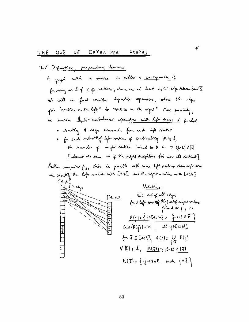
83

84

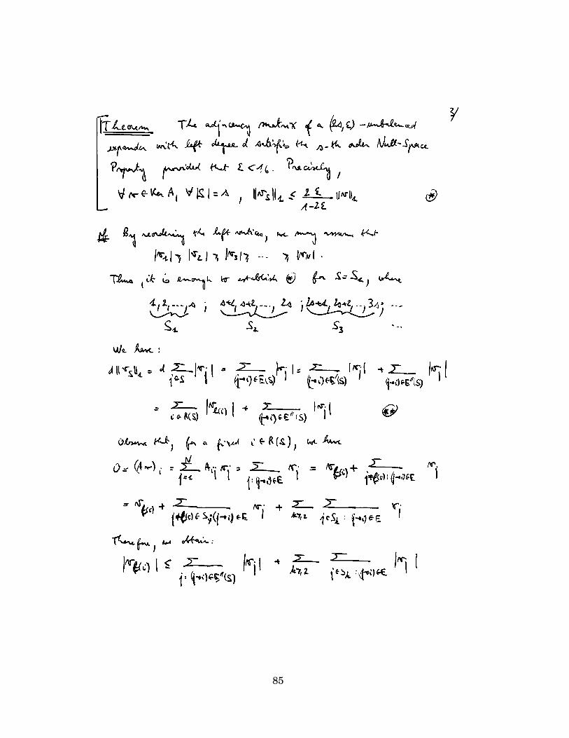
85

86

87

88

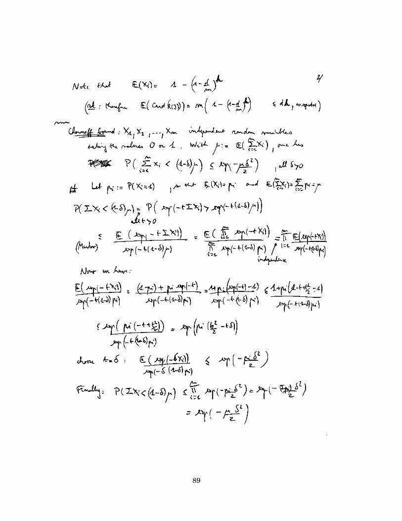
89

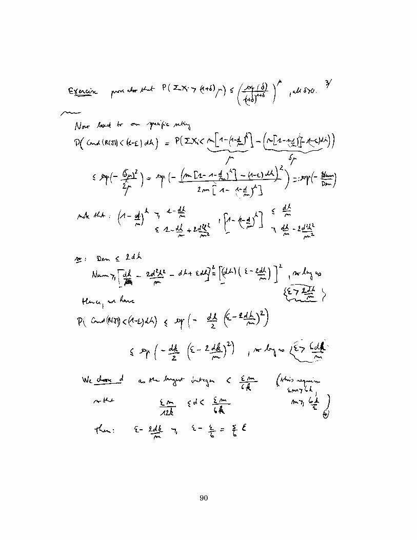
90

91

92

Chapter 13

Orthogonal Matching Pursuit

See the following handwritten notes.

93

94

95

96

97

Chapter 14

ROMP and CoSaMP

98

Appendix 1: Some Theorems andTheir Proofs

Proof of Borsuk–Ulam Theorem: to come

Proof of Krein–Mil’man Theorem: to come

Proof of Farkas’ Lemma: to come

Proof of Karush–Kuhn–Tucker: to come

It is a rather common problem to minimize a function defined by a maximum, e.g. when welook at a best approximation. The following theorem generalizes some characterizations ofbest approximations or of minimal projections. Roughly speaking, it allows the reductionof the domain of maximization.

Theorem 14.1. Let f be a function defined on C × K where C is a convex set and K isa compact set. We assume the convexity of f(•, y) for any y ∈ K, the continuity of f(x, •)for any x ∈ C and the equicontinuity of (f(•, y))y∈K at some point x∗ ∈ C. The followingpropositions are equivalent:

(i) ∃x ∈ C : maxy∈K

f(x, y) < maxy∈K

f(x∗, y),

(ii) ∃x ∈ C : ∀ z ∈ K satisfying f(x∗, z) = maxy∈K

f(x∗, y), one has f(x, z) < f(x∗, z).

If in addition the set K is convex and the function f(x∗, •) is convex, the propositions (i)–(ii)

99

are also equivalent to

(iii) ∃x ∈ C : ∀ z ∈ Ex(K) satisfying f(x∗, z) = maxy∈K

f(x∗, y), one has f(x, z) < f(x∗, z).

Proof. The implications (i)⇒(ii) and (ii)⇒(iii) are straightforward.For x ∈ C, we consider the non-empty compact subset Dx of K defined by

Dx :=z ∈ K : f(x, z) = max

y∈Kf(x, y)

.

Let us assume that (ii) holds, i.e. that there exists x ∈ K for which

m := maxz∈Dx∗

f(x, z) < maxy∈K

f(x∗, y) =: M.

We consider the open neighborhood of Dx∗ defined by O :=y ∈ K : f(x, y) < (m+M)/2

.

For y ∈ K \ O ⊆ K \Dx∗ , we have f(x∗, y) < M , and we set

m′ := maxy∈K\O

f(x∗, y) < M.

Let t > 0 be small enough for |f(x∗+ t(x−x∗), y)− f(x∗, y)| < M −m′ to hold for any y ∈ K.We then get

y ∈ K \ O ⇒ f(x∗ + t(x− x∗), y) < M −m′ + f(x∗, y) ≤M,

y ∈ O ⇒ f((1− t)x∗ + tx, y) ≤ (1− t)f(x∗, y) + tf(x, y) ≤ (1− t)M + t(m+M)/2 < M.

We have therefore obtained (i) in the form maxy∈K

f((1− t)x∗ + tx, y) < M .

Let us now assume that K is a convex set and that f(x∗, •) is a convex function. It followsthat Dx∗ is an extreme set of K, hence that Ex(Dx∗) = Ex(K) ∩ Dx∗ . The property (iii),assumed to hold, now reads, for some x ∈ C,

∀ z ∈ Ex(Dx∗), f(x, z) < M.

Thus, for any y ∈ Dx∗ ⊆ co[Dx∗ ] = co[Ex(Dx∗)], we have f(x, y) ≤ M . We aim at provingproperty (ii) as the statement that the set S :=

y ∈ Dx∗ : f(x∗, y) = M

is empty. If it was

not, due to the compactness of S, we would have Ex(S) 6= ∅. But since S is an extreme setof Dx∗ , we have Ex(S) = Ex(Dx∗) ∩ S, which is empty.

Corollary 14.2. Let V be a subspace of a normed space X. For x ∈ X and v∗ ∈ V , one has[‖x− v∗‖ = inf

v∈V‖x− v‖

]⇐⇒

[∀ v ∈ V, ∃λ ∈ Ex(BX∗) : λ(x− v) ≥ λ(x− v∗) = ‖x− v∗‖

].

100

Appendix 2: Hints to the Exercises

Chapter 1. Ex.1: need to prove that B>B is invertible; observe that B>Bx = 0 impliesthat ‖Bx‖22 = 〈B>Bx, x〉 = 0 and in turn that x = 0 because B is injective by the ranktheorem. Ex.2: write x = Ux′, where x′ is s-sparse and Ui,j = 1 for i ≤ j, 0 otherwise;recover x′ by minimizing ‖U−1z‖1 subject to Az = y; calculate U−1z. Ex.3: reduce theproblem to the case Ω = π; define a 2π-periodic function g by g|[−π,π] = f|[−π,π] and calcu-late its Fourier coefficients; use the inversion formula to express f in terms of g. Ex.4:dimension considerations. Ex.5: for y 6= y′ ∈ Rm, consider the errors e := (By′ − By)J1,sK

and e′ = (By − By′)Js+1,2sK. Ex.6: N=512;m=128;s=20; y=rand(m,1); A=randn(m,N);

[V,D]=eig(A’*A);B=V*[randn(N-m,m);zeros(m,m)]; permN=randperm(N);supp

=sort(permN(1:s)); e=zeros(N,1);e(supp)=rand(s,1); estar=l1eq pd(x,A,[]

,A*x); ystar=B\(x-estar); norm(y-ystar) Ex.7: ∀u ∈ kerA \ 0, |supp(u)|w >

2 max|S|≤s |supp(u) ∩ S|w.

Chapter 2. Ex.1: if f : S → N is an injection, then extend[f |f(S)

]−1 to obtain a surjectiong : N → S; if g : N → S is a surjection, then choose f(x) ∈ g−1(x) for all x ∈ S to definean injection f : S → N. Ex.2: ... Ex.3: F : x ∈ Σ[1:s] 7→ f(x) − f(−x) ∈ Rm is continu-ous and antipodal; if s > m, then Borsuk–Ulam theorem yields a contradiction. Ex.4: ifSn(1) and Sn(2) are the unit spheres in Rn+1 relative to two norms ‖ · ‖(1) and ‖ · ‖(2), thencompose a continuous antipodal map from Sn(2) to Rn with the map x ∈ Sn(1) →

x‖x‖(2)

∈ Sn(2)

to obtain a continuous and antipodal map from Sn(1) to Rn. Ex.5: starting form G, defineF by F (x) := G(x) − G(−x) and apply the first formulation; starting form F , apply thesecond formulation and use antipodality. Ex.6: the concatenation of two weighted planarnetworks is a weighted planar network. Ex.7: start by factoring out the term (1 − xj)n

for the j-th column and(ni

)for the i-th row. Ex.8: the condition necessary and sufficient

is detM[1:k] 6= 0, all k ∈ [1 : n − 1], which is satisfied by totally positive matrices; New-ton’s interpolation yields p(x) =

∑nk=0[x0, . . . , xk]p · (x − x0) · · · (x − xk) for p ∈ Pn, where

the divided difference [x0, . . . , xk]p is the coefficient on xk in the polynomial of degree ≤ k

101

interpolating p at x0, . . . , xk; specify p(x) = xj and x = xi. Ex.9: N=512; m=128; s=20;

R=sort(rand(1,N)); for i=1:m, A(i,:)=R.ˆ(i-1); end; permN=randperm(N);

supp=sort(permN(1:s)); x=zeros(N,1); x(supp)=rand(s,1); y=A*x; x1=A\y;xstar=l1eq pd(x1,A,[],y,1e-3);

Chapter 3. Ex.1: the eigenvectors are the [1, ei2πj/N , . . . , ei2πj(N−1)/N ]>, j ∈ [0 : N − 1],and the eigenvalues are the discrete Fourier coefficients of [c0, . . . , cN−1]>. Ex.2: subtracta variable x to every entry, then the determinant is a linear function to be evaluated attwo particular values for x. Ex.3: write down the definitions of u ∗ v(j) and of (u ∗ v)(j),manipulate the sums to obtain u(j) · v(j) and N u · v(j). Ex.4: P=[1]; for k=1:20,

P=conv(P,[1,-k]); end; P(2)=P(2)+10ˆ(-8); roots(P)’; Ex.5: N=500; s=18;

supp=sort(randsample(N,s));x=randn(N,1)/10ˆ4;x(supp)=randn(s,1); xhat=

fft(x);y=xhat(1:2*s);A=toeplitz(y(s:2*s-1),y(s:-1:1));phat=zeros(N,1);

phat(1)=1; phat(2:s+1)=-A\y(s+1:2*s); p=ifft(phat); [sorted p,ind]=sort

(abs(p)); rec supp=sort(ind(1:s)); [supp’;rec supp’]

Chapter 4. Ex.1: use the triangle inequality ‖x+y‖qq ≤ ‖x‖qq+‖y‖qq and Holder’s inequality‖x‖qq + ‖y‖qq ≤ [1 + 1]1−q[‖x‖q + ‖y‖q]q to derive ‖x+y‖q ≤ 2(1−q)/q[‖x‖q + ‖y‖q]; for ‖x‖q = 1,write ‖(T + U)x‖q ≤ 2(1−q)/q[‖Tx‖q + ‖Ux‖q] ≤ 2(1−q)/q[‖T‖q + ‖U‖q] and take the supre-mum. Ex.2: if v ∈ Σ2s ∩ kerA, then take S to be an index set of s largest absolute-valuecomponents of v to get ‖vS‖qq ≥ ‖vS‖

qq. Ex.3: take a (2s) × (2s + 1) matrix whose kernel

is spanned by [a, . . . , a︸ ︷︷ ︸s

, 1, . . . , 1︸ ︷︷ ︸s+1

]> with a := (1 + 1/s)1/q. Ex.4: to prove the strengthened

Minimality Property, apply the strengthened Null-Space Property with v = x− z, to provethe strengthened Null-Space Property, apply the strengthened Minimality Property withx = vS and z = −vS , observe that c = C.

Chapter 5. Ex.1: imitate the proof of Proposition 5.1. Ex.2: if S is the index set of slargest absolute-value components of x, then the best s-term approximation to x is providedby xS independently of q. Ex.3: to establish Instance Optimality from the Null-SpaceProperty, define the reconstruction map by g(y) ∈ argminσs(z)1 : Az = y, keep in mindthe inequality σs(a + b)1 ≤ σs(a)1 + σ1(b), a,b ∈ RN , conversely, to establish the Null-Space Property from Instance Optimality, given v ∈ kerA, choose an index set S so that‖vS‖1 = σ2s(v)1, and split vS as vS = v1 + v2 with v1,v2 ∈ Σs, then justify that ‖v‖1 =‖v2 + vS − g(A(v2 + vS))‖1 ≤ Cσs(v2 + vS)1 = C‖vS‖1 = Cσ2s(v)1. Ex.4: adapt Ex.3 toobserve that, if A exhibits Instance Optimality of order s, then there is a constant c < 1such that ‖vS‖2 ≤ c‖v‖2 for all v ∈ kerA and |S| ≤ s, given the canonical basis (e1, . . . , eN )of RN and given an orthonormal basis (v1, . . . ,vN−m) of kerA, we get

∑N−mi=1 〈ej ,vi〉2 =

102

〈∑N−m

i=1 〈ej ,vi〉vi, ej〉 ≤ c‖∑N−m

i=1 〈ej ,vi〉vi‖2 ≤ c‖ej‖2 = c, sum over j ∈ [1 : N ] and invertthe summations to obtain N −m ≤ cN .

Chapter 6. Ex.2: minimize t subject to −t ≤ xi − vi ≤ t and 〈v,u1〉 = 0, . . . , 〈v,uk〉 = 0,where (u1, . . . ,uk) denotes a basis of the orthogonal complement V⊥ of V in Rn. Ex.5:minimize

∑tj subject to z2

re,j + z2im,j ≤ t2j , Arezre −Aimzim = yre, Arezim +Aimzre = yim.

103

Bibliography

[1] S. Boyd, L. Vandenberghe. Convex Optimization. Cambridge University Press.

[2] E. Candes, J. Romberg. `1-magic: Recovery of Sparse Signals via Convex Programing.Available online.

[3] R. Baraniuk, M. Davenport, R. DeVore, M. Wakin. A Simple Proof of the RestrictedIsometry Property for Random Matrices, Constructive Approximation, ...

[4] Emmanuel Candes. Compressive Sampling, Proceeding of the INternational Congressof Mathematicians, Madrid, Spain, 2006.

[5] Emmanuel Candes. The Restricted Isometry Property and Its Implication for Com-pressed Sensing, Comptes Rendus de l’Academie des Sciences, Paris, Serie I, 346,589–592, 2008.

[6] Emmanuel Candes, Justin Romberg, Terence Tao. Robust Uncertainty Principles: Ex-act Signal Reconstruction from Highly Incomplete Frequency Information, ....

[7] Emmanuel Candes, Justin Romberg, Terence Tao. Stabl Signal Recovery from Incom-plete and Inaccurate Measurements, ....

[8] Emmanuel Candes, Terence Tao. Decoding by Linear Programing, ...

[9] Emmanuel Candes, Terence Tao. Near Optimal Signal Recovery from Random Projec-tions: Universal Encoding Strategies?, ...

[10] E. Candes, M. Wakin, S. Boyd. Enhancing Sparsity by Reweighted `1 Minimization, ...

[11] Venkat Chandar. A Negative Result Concerning Explicit Matrices with the RestrictedIsometry Property, ...

[12] Rick Chartrand, Valentina Stavena. Restricted Isometry Properties and NonconvexCompressive Sensing, ...

104

[13] Albert Cohen, Wolfgang Dahmen, Ronald DeVore. Compressed Sensing and best k-term approximation, ...

[14] Albert Cohen, Wolfgang Dahmen, Ronald DeVore. Instance Optimal Decoding byThresholding in Compressed Sensing, ...

[15] I. Daubechies, R. DeVore, M. Fornasier, C. Sinan Gunturk. Iteratively Re-WeightedLeast Squares Minimization for Sparse Recovery, ...

[16] Michael Davies, Remi Gribonval. Restricted Isometry Constants where `p sparse re-covery can fail for 0 < p ≤ 1, Preprint submitted to ... .

[17] Ronald DeVore, Deterministic Constructions of Compressed Sensing Matrices, ...

[18] Ronald DeVore, Guergana Petrova, Przemyslaw Wojtaszczyk. Instance-Optimality inProbability with an `1-Minimization Decoder, ...

[19] David Donoho. Compressed Sensing, ...

[20] David Donoho, For Most Large Underdetermined Systems of Linear Equations theMinimal `1-norm Solution is also the Sparsest Solution, ...

[21] David Donoho, For Most Large Underdetermined Systems of Equations, the Minimal`1-norm Near-Solution Approximates the Sparsest Near-Solution, ...

[22] David Donoho, Jared Tanner. Counting Faces of Randomly-Projected Polytopes whenthe Projection Radically Lowers Dimension, ...

[23] David Donoho, Jared Tanner. Counting the Faces of Randomly-Projected Hypercubesand Orthants, with Applications, ...

[24] S. Foucart, M.-J. Lai. Sparsest solutions of underdetermined linear systems via `q-minimization for 0 < q ≤ 1, Applied and Computational Harmonic Analysis, in press.

[25] Jean-Jacques Fuchs, On Sparse Representations in Arbitrary Redundant Bases, ...

[26] R. Berinde, A. Gilbert, P. Indyk, H. Karloff, J. Strauss. Combining Geometry andCombinatorics: a Unified Approach to Sparse Signal Recovery, ...

[27] R. Gribonval, M. Nielsen. Highly Sparse Representations from Dictionaries areUnique and Independent of the Sparsness Measure, ...

[28] B. S. Kashin, V. N. Temlyakov. A Remark on Compressed Sensing

105

[29] Basarab Matei, Yves Meyer. A Variant on the Compressed Sensing of EmmanuelCandes, ...

[30] D. Needell, J. Tropp. CoSamp: Iteravtive Signal Recovery from Incomplete and Inac-curate Samples, ...

[31] D. Needell, R. Vershynin. Uniform Uncertainty Principle and Signal Recovery viaRegularized Orthogonal Matching Pursuit, ...

[32] D. Needell, R. Vershynin. Signal Recovery from Incomplete and Inaccurate Measure-ments vis Regularized Orthogonal Matching Pursuit, ...

[33] Yaakov Tsaig, David Donoho. Extensions of Compressed Sensing, ...

[34] P. Wojtaszczyk. Stability and Instance Optimality for Gaussian Measurements inCompressed Sensing, ...

106