notes for ece 467 communication network analysis - university of

Notes for ECE 467

Communication Network Analysis

Bruce Hajek

December 15, 2006

c© 2006 by Bruce Hajek

All rights reserved. Permission is hereby given to freely print and circulate copies of these notes so long as the notes are left

intact and not reproduced for commercial purposes. Email to [email protected], pointing out errors or hard to understand

passages or providing comments, is welcome.

Contents

1 Countable State Markov Processes 31.1 Example of a Markov model . . . . . . . . . . . . . . . . . . . . . . . . . . . . . . . . 31.2 Definition, Notation and Properties . . . . . . . . . . . . . . . . . . . . . . . . . . . . 51.3 Pure-Jump, Time-Homogeneous Markov Processes . . . . . . . . . . . . . . . . . . . 61.4 Space-Time Structure . . . . . . . . . . . . . . . . . . . . . . . . . . . . . . . . . . . 81.5 Poisson Processes . . . . . . . . . . . . . . . . . . . . . . . . . . . . . . . . . . . . . . 121.6 Renewal Theory . . . . . . . . . . . . . . . . . . . . . . . . . . . . . . . . . . . . . . 14

1.6.1 Renewal Theory in Continuous Time . . . . . . . . . . . . . . . . . . . . . . . 161.6.2 Renewal Theory in Discrete Time . . . . . . . . . . . . . . . . . . . . . . . . 17

1.7 Classification and Convergence of Discrete State Markov Processes . . . . . . . . . . 171.7.1 Examples with finite state space . . . . . . . . . . . . . . . . . . . . . . . . . 171.7.2 Discrete Time . . . . . . . . . . . . . . . . . . . . . . . . . . . . . . . . . . . . 201.7.3 Continuous Time . . . . . . . . . . . . . . . . . . . . . . . . . . . . . . . . . . 22

1.8 Classification of Birth-Death Processes . . . . . . . . . . . . . . . . . . . . . . . . . . 241.9 Time Averages vs. Statistical Averages . . . . . . . . . . . . . . . . . . . . . . . . . . 261.10 Queueing Systems, M/M/1 Queue and Little’s Law . . . . . . . . . . . . . . . . . . . 271.11 Mean Arrival Rate, Distributions Seen by Arrivals, and PASTA . . . . . . . . . . . . 301.12 More Examples of Queueing Systems Modeled as Markov Birth-Death Processes . . 321.13 Method of Phases and Quasi Birth-Death Processes . . . . . . . . . . . . . . . . . . 341.14 Markov Fluid Model of a Queue . . . . . . . . . . . . . . . . . . . . . . . . . . . . . 361.15 Problems . . . . . . . . . . . . . . . . . . . . . . . . . . . . . . . . . . . . . . . . . . 37

2 Foster-Lyapunov stability criterion and moment bounds 452.1 Stability criteria for discrete time processes . . . . . . . . . . . . . . . . . . . . . . . 452.2 Stability criteria for continuous time processes . . . . . . . . . . . . . . . . . . . . . 532.3 Problems . . . . . . . . . . . . . . . . . . . . . . . . . . . . . . . . . . . . . . . . . . 57

3 Queues with General Interarrival Time and/or Service Time Distributions 613.1 The M/GI/1 queue . . . . . . . . . . . . . . . . . . . . . . . . . . . . . . . . . . . . . 61

3.1.1 Busy Period Distribution . . . . . . . . . . . . . . . . . . . . . . . . . . . . . 633.1.2 Priority M/GI/1 systems . . . . . . . . . . . . . . . . . . . . . . . . . . . . . 64

3.2 The GI/M/1 queue . . . . . . . . . . . . . . . . . . . . . . . . . . . . . . . . . . . . . 663.3 The GI/GI/1 System . . . . . . . . . . . . . . . . . . . . . . . . . . . . . . . . . . . . 683.4 Kingman’s Bounds for GI/GI/1 Queues . . . . . . . . . . . . . . . . . . . . . . . . . 693.5 Stochastic Comparison with Application to GI/GI/1 Queues . . . . . . . . . . . . . 71

iii

3.6 GI/GI/1 Systems with Server Vacations, and Application to TDM and FDM . . . . 733.7 Effective Bandwidth of a Data Stream . . . . . . . . . . . . . . . . . . . . . . . . . . 753.8 Problems . . . . . . . . . . . . . . . . . . . . . . . . . . . . . . . . . . . . . . . . . . 78

4 Multiple Access 834.1 Slotted ALOHA with Finitely Many Stations . . . . . . . . . . . . . . . . . . . . . . 834.2 Slotted ALOHA with Infinitely Many Stations . . . . . . . . . . . . . . . . . . . . . 854.3 Bound Implied by Drift, and Proof of Proposition 4.2.1 . . . . . . . . . . . . . . . . 874.4 Probing Algorithms for Multiple Access . . . . . . . . . . . . . . . . . . . . . . . . . 90

4.4.1 Random Access for Streams of Arrivals . . . . . . . . . . . . . . . . . . . . . 924.4.2 Delay Analysis of Decoupled Window Random Access Scheme . . . . . . . . 92

4.5 Problems . . . . . . . . . . . . . . . . . . . . . . . . . . . . . . . . . . . . . . . . . . 93

5 Stochastic Network Models 995.1 Time Reversal of Markov Processes . . . . . . . . . . . . . . . . . . . . . . . . . . . . 995.2 Circuit Switched Networks . . . . . . . . . . . . . . . . . . . . . . . . . . . . . . . . . 1015.3 Markov Queueing Networks (in equilibrium) . . . . . . . . . . . . . . . . . . . . . . . 104

5.3.1 Markov server stations in series . . . . . . . . . . . . . . . . . . . . . . . . . . 1045.3.2 Simple networks of MS stations . . . . . . . . . . . . . . . . . . . . . . . . . . 1055.3.3 A multitype network of MS stations with more general routing . . . . . . . . 107

5.4 Problems . . . . . . . . . . . . . . . . . . . . . . . . . . . . . . . . . . . . . . . . . . 109

6 Calculus of Deterministic Constraints 1136.1 The (σ, ρ) Constraints and Performance Bounds for a Queue . . . . . . . . . . . . . 1136.2 f -upper constrained processes . . . . . . . . . . . . . . . . . . . . . . . . . . . . . . 1156.3 Service Curves . . . . . . . . . . . . . . . . . . . . . . . . . . . . . . . . . . . . . . . 1176.4 Problems . . . . . . . . . . . . . . . . . . . . . . . . . . . . . . . . . . . . . . . . . . 120

7 Graph Algorithms 1237.1 Maximum Flow Problem . . . . . . . . . . . . . . . . . . . . . . . . . . . . . . . . . . 1237.2 Problems . . . . . . . . . . . . . . . . . . . . . . . . . . . . . . . . . . . . . . . . . . 124

8 Flow Models in Routing and Congestion Control 1278.1 Convex functions and optimization . . . . . . . . . . . . . . . . . . . . . . . . . . . . 1278.2 The Routing Problem . . . . . . . . . . . . . . . . . . . . . . . . . . . . . . . . . . . 1288.3 Utility Functions . . . . . . . . . . . . . . . . . . . . . . . . . . . . . . . . . . . . . . 1338.4 Joint Congestion Control and Routing . . . . . . . . . . . . . . . . . . . . . . . . . . 1348.5 Hard Constraints and Prices . . . . . . . . . . . . . . . . . . . . . . . . . . . . . . . . 1358.6 Decomposition into Network and User Problems . . . . . . . . . . . . . . . . . . . . 1368.7 Specialization to pure congestion control . . . . . . . . . . . . . . . . . . . . . . . . . 1398.8 Fair allocation . . . . . . . . . . . . . . . . . . . . . . . . . . . . . . . . . . . . . . . 1418.9 A Network Evacuation Problem . . . . . . . . . . . . . . . . . . . . . . . . . . . . . . 1428.10 Braess Paradox . . . . . . . . . . . . . . . . . . . . . . . . . . . . . . . . . . . . . . . 1428.11 Further reading and notes . . . . . . . . . . . . . . . . . . . . . . . . . . . . . . . . . 1448.12 Problems . . . . . . . . . . . . . . . . . . . . . . . . . . . . . . . . . . . . . . . . . . 144

iv

9 Dynamic Network Control 1499.1 Dynamic programming . . . . . . . . . . . . . . . . . . . . . . . . . . . . . . . . . . . 1499.2 Dynamic Programming Formulation . . . . . . . . . . . . . . . . . . . . . . . . . . . 1509.3 The Dynamic Programming Optimality Equations . . . . . . . . . . . . . . . . . . . 1529.4 Problems . . . . . . . . . . . . . . . . . . . . . . . . . . . . . . . . . . . . . . . . . . 156

10 Solutions 161

v

Preface

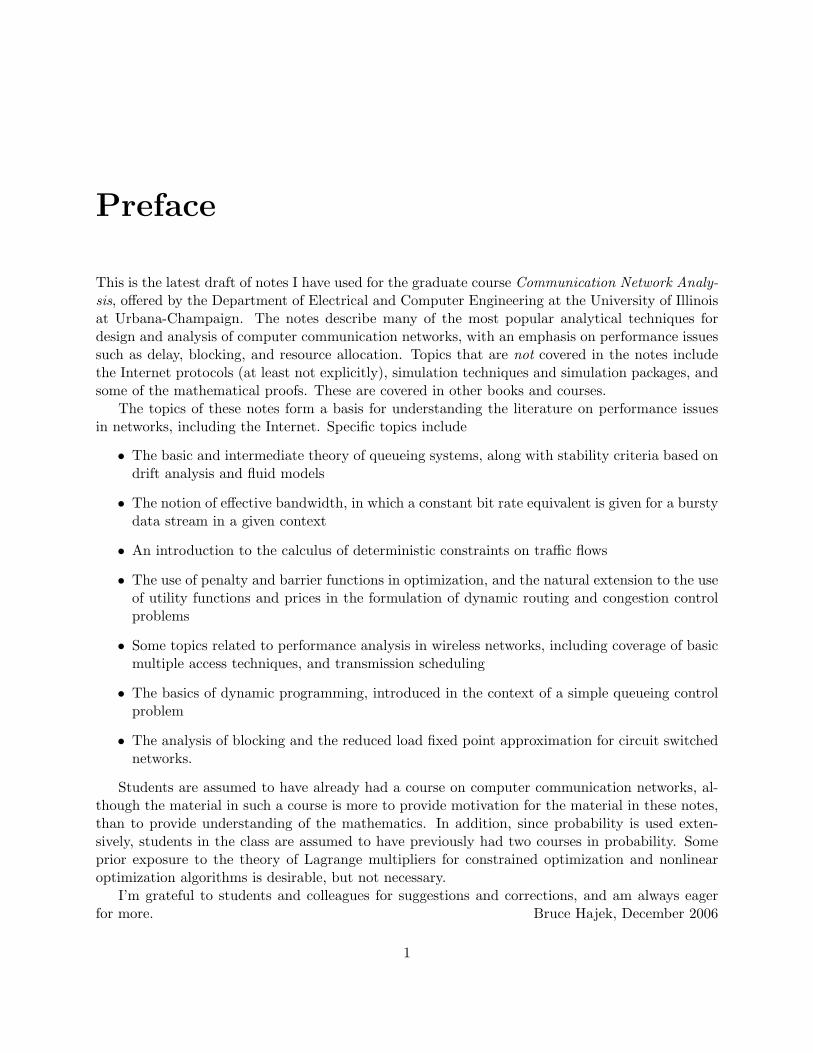
This is the latest draft of notes I have used for the graduate course Communication Network Analy-sis, offered by the Department of Electrical and Computer Engineering at the University of Illinoisat Urbana-Champaign. The notes describe many of the most popular analytical techniques fordesign and analysis of computer communication networks, with an emphasis on performance issuessuch as delay, blocking, and resource allocation. Topics that are not covered in the notes includethe Internet protocols (at least not explicitly), simulation techniques and simulation packages, andsome of the mathematical proofs. These are covered in other books and courses.

The topics of these notes form a basis for understanding the literature on performance issuesin networks, including the Internet. Specific topics include

• The basic and intermediate theory of queueing systems, along with stability criteria based ondrift analysis and fluid models

• The notion of effective bandwidth, in which a constant bit rate equivalent is given for a burstydata stream in a given context

• An introduction to the calculus of deterministic constraints on traffic flows

• The use of penalty and barrier functions in optimization, and the natural extension to the useof utility functions and prices in the formulation of dynamic routing and congestion controlproblems

• Some topics related to performance analysis in wireless networks, including coverage of basicmultiple access techniques, and transmission scheduling

• The basics of dynamic programming, introduced in the context of a simple queueing controlproblem

• The analysis of blocking and the reduced load fixed point approximation for circuit switchednetworks.

Students are assumed to have already had a course on computer communication networks, al-though the material in such a course is more to provide motivation for the material in these notes,than to provide understanding of the mathematics. In addition, since probability is used exten-sively, students in the class are assumed to have previously had two courses in probability. Someprior exposure to the theory of Lagrange multipliers for constrained optimization and nonlinearoptimization algorithms is desirable, but not necessary.

I’m grateful to students and colleagues for suggestions and corrections, and am always eagerfor more. Bruce Hajek, December 2006

1

Chapter 1

Countable State Markov Processes

1.1 Example of a Markov model

Consider a two-stage pipeline as pictured in Figure 1.1. Some assumptions about it will be madein order to model it as a simple discrete time Markov process, without any pretension of modelinga particular real life system. Each stage has a single buffer. Normalize time so that in one unitof time a packet can make a single transition. Call the time interval between k and k + 1 the kth“time slot,” and assume that the pipeline evolves in the following way during a given slot.

If at the beginning of the slot, there are no packets in stage one, then a new packet arrives to stageone with probability a, independently of the past history of the pipeline and of the outcomeat state two.

If at the beginning of the slot, there is a packet in stage one and no packet in stage two, then thepacket is transfered to stage two with probability d1.

If at the beginning of the slot, there is a packet in stage two, then the packet departs from thestage and leaves the system with probability d2, independently of the state or outcome ofstage one.

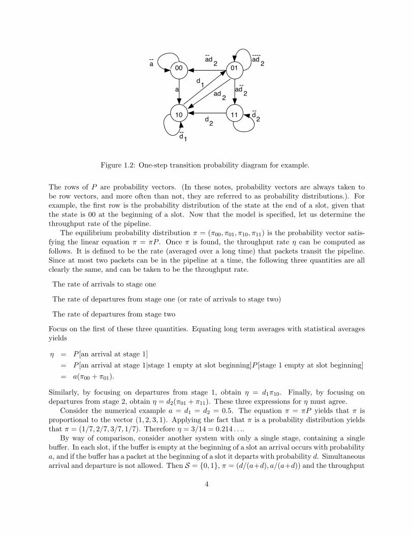
These assumptions lead us to model the pipeline as a discrete-time Markov process with thestate space S = 00, 01, 10, 11, transition probability diagram shown in Figure 1.2 (using thenotation x = 1− x) and one-step transition probability matrix P given by

P =

a 0 a 0

ad2 ad2 ad2 ad2

0 d1 d1 00 0 d2 d2

a dd1 2

Figure 1.1: A two-stage pipeline

3

1

00

10 11

01

a

a

d

d1 ad 2

ad 2

d2d2

ad 2

ad 2

--

--

--

--

--

--

--

Figure 1.2: One-step transition probability diagram for example.

The rows of P are probability vectors. (In these notes, probability vectors are always taken tobe row vectors, and more often than not, they are referred to as probability distributions.). Forexample, the first row is the probability distribution of the state at the end of a slot, given thatthe state is 00 at the beginning of a slot. Now that the model is specified, let us determine thethroughput rate of the pipeline.

The equilibrium probability distribution π = (π00, π01, π10, π11) is the probability vector satis-fying the linear equation π = πP . Once π is found, the throughput rate η can be computed asfollows. It is defined to be the rate (averaged over a long time) that packets transit the pipeline.Since at most two packets can be in the pipeline at a time, the following three quantities are allclearly the same, and can be taken to be the throughput rate.

The rate of arrivals to stage one

The rate of departures from stage one (or rate of arrivals to stage two)

The rate of departures from stage two

Focus on the first of these three quantities. Equating long term averages with statistical averagesyields

η = P [an arrival at stage 1]= P [an arrival at stage 1|stage 1 empty at slot beginning]P [stage 1 empty at slot beginning]= a(π00 + π01).

Similarly, by focusing on departures from stage 1, obtain η = d1π10. Finally, by focusing ondepartures from stage 2, obtain η = d2(π01 + π11). These three expressions for η must agree.

Consider the numerical example a = d1 = d2 = 0.5. The equation π = πP yields that π isproportional to the vector (1, 2, 3, 1). Applying the fact that π is a probability distribution yieldsthat π = (1/7, 2/7, 3/7, 1/7). Therefore η = 3/14 = 0.214 . . ..

By way of comparison, consider another system with only a single stage, containing a singlebuffer. In each slot, if the buffer is empty at the beginning of a slot an arrival occurs with probabilitya, and if the buffer has a packet at the beginning of a slot it departs with probability d. Simultaneousarrival and departure is not allowed. Then S = 0, 1, π = (d/(a+d), a/(a+d)) and the throughput

4

rate is ad/(a+d). The two-stage pipeline with d2 = 1 is essentially the same as the one-stage system.In case a = d = 0.5, the throughput rate of the single stage system is 0.25, which as expected issomewhat greater than that of the two-stage pipeline.

1.2 Definition, Notation and Properties

Having given an example of a discrete state Markov process, we now digress and give the formaldefinitions and some of the properties of Markov processes. Let T be a subset of the real numbersR and let S be a finite or countably infinite set. A collection of S–valued random variables (X(t) :t ∈ T) is a discrete-state Markov process with state space S if

P [X(tn+1) = in+1|X(tn) = in, . . . , X(t1) = i1] = P [X(tn+1) = in+1|X(tn) = in] (1.1)

whenever t1 < t2 < . . . < tn+1 are in T,ii, i2, ..., in+1 are in S, andP [X(tn) = in, . . . , X(t1) = i1] > 0.

(1.2)

Set pij(s, t) = P [X(t) = j|X(s) = i] and πi(t) = P [X(t) = i]. The probability distributionπ(t) = (πi(t) : i ∈ S) should be thought of as a row vector, and can be written as one once Sis ordered. Similarly, H(s, t) defined by H(s, t) = (pij(s, t) : i, j ∈ S) should be thought of as amatrix. Let e denote the column vector with all ones, indexed by S. Since π(t) and the rows ofH(s, t) are probability vectors for s, t ∈ T and s ≤ t, it follows that π(t)e = 1 and, H(s, t)e = e.

Next observe that the marginal distributions π(t) and the transition probabilities pij(s, t) de-termine all the finite dimensional distributions of the Markov process. Indeed, given

t1 < t2 < . . . < tn in T,ii, i2, ..., in ∈ S (1.3)

one writes

P [X(t1) = i1, . . . , X(tn) = in] =P [X(t1) = i1, . . . , X(tn−1) = in−1]P [X(tn) = in|X(t1) = i1, . . . , X(tn−1) = in−1]

= P [X(t1) = i1, . . . , X(tn−1) = in−1]pin−1in(tn−1, tn)

Application of this operation n− 2 more times yields that

P [X(t1) = i1, X(t2) = i2, . . . , X(tn) = in] = πi1(t1)pi1i2(t1, t2) . . . pin−1in(tn−1, tn), (1.4)

which shows that the finite dimensional distributions of X are indeed determined by (π(t)) and(pij(s, t)). From this and the definition of conditional probabilities it follows by straight substitutionthat

P [X(tj) = ij , for 1 ≤ j ≤ n + l|X(tn) = in] = (1.5)P [X(tj) = ij , for 1 ≤ j ≤ n|X(tn) = in]P [X(tj) = ij , for n ≤ j ≤ n + l|X(tn) = in]

whenever P [X(tn) = in] > 0. Property (1.5) is equivalent to the Markov property. Note in additionthat it has no preferred direction of time, simply stating that the past and future are conditionally

5

independent given the present. It follows that if X is a Markov process, the time reversal of Xdefined by X(t) = X(−t) is also a Markov process.

A Markov process is time homogeneous if pij(s, t) depends on s and t only through t − s. Inthat case we write pij(t− s) instead of pij(s, t), and Hij(t− s) instead of Hij(s, t).

Recall that a random process is stationary if its finite dimensional distributions are invariantwith respect to translation in time. Referring to (1.4), we see that a time-homogeneous Markovprocess is stationary if and only if its one dimensional distributions π(t) do not depend on t. If, inour example of a two-stage pipeline, it is assumed that the pipeline is empty at time zero and thata 6= 0, then the process is not stationary (since π(0) = (1, 0, 0, 0) 6= π(1) = (1 − a, 0, a, 0)), eventhough it is time homogeneous. On the other hand, a Markov random process that is stationary istime homogeneous.

Computing the distribution of X(t) by conditioning on the value of X(s) yields that πj(t) =∑i P [X(s) = i,X(t) = j] =

∑i πi(s)pij(s, t), which in matrix form yields that π(t) = π(s)H(s, t)

for s, t ∈ T, s ≤ t. Similarly, given s < τ < t, computing the conditional distribution of X(t) givenX(s) by conditioning on the value of X(τ) yields

H(s, t) = H(s, τ)H(τ, t) s, τ, t ∈ T, s < τ < t. (1.6)

The relations (1.6) are known as the Chapman-Kolmogorov equations.If the Markov process is time-homogeneous, then π(s + τ) = π(s)H(τ) for s, s + τ ∈ T and

τ ≥ 0. A probability distribution π is called an equilibrium (or invariant) distribution if πH(τ) = πfor all τ ≥ 0.

Repeated application of the Chapman-Kolmogorov equations yields that pij(s, t) can be ex-pressed in terms of transition probabilities for s and t close together. For example, considerMarkov processes with index set the integers. Then H(n, k + 1) = H(n, k)P (k) for n ≤ k, whereP (k) = H(k, k + 1) is the one-step transition probability matrix. Fixing n and using forward re-cursion starting with H(n, n) = I, H(n, n + 1) = P (n), H(n, n + 2) = P (n)P (n + 1), and so forthyields

H(n, l) = P (n)P (n + 1) · · ·P (l − 1)

In particular, if the process is time-homogeneous then H(k) = P k for all k for some matrix P , andπ(l) = P l−kπ(k) for l ≥ k. In this case a probability distribution π is an equilibrium distributionif and only if πP = π.

In the next section, processes indexed by the real line are considered. Such a process can bedescribed in terms of p(s, t) with t− s arbitrarily small. By saving only a linearization, the conceptof generator matrix arises naturally.

1.3 Pure-Jump, Time-Homogeneous Markov Processes

Let S be a finite or countably infinite set, and let 4 6∈ S. A pure-jump function is a functionx : R+ → S ∪ 4 such that there is a sequence of times, 0 = τ0 < τ1 < . . . , and a sequence ofstates, s0, s1, . . . with si ∈ S, and si 6= si+1, i ≥ 0, so that

x(t) =

si if τi ≤ t < τi+1 i ≥ 04 if t ≥ τ∗

(1.7)

where τ∗ = limi→∞ τi. If τ∗ is finite it is said to be the explosion time of the function x. Theexample corresponding to S = 0, 1, . . ., τi = i/(i + 1) and si = i is pictured in Fig. 1.3. Note

6

x(t)

! 10 2. . . "

t! ! !

Figure 1.3: Sample pure-jump function with an explosion time

1 2

3

11

1

0.5

0.5

Figure 1.4: Transition rate diagram for a continuous time Markov process

that τ∗ = 1 for this example. A pure-jump Markov process (Xt : t ≥ 0) is a Markov process suchthat, with probability one, its sample paths are pure-jump functions.

Let Q = (qij : i, j ∈ S) be such that

qij ≥ 0 i, j ∈ S, i 6= jqii = −

∑j∈S,j 6=i qij i ∈ S.

(1.8)

An example for state space S = 1, 2, 3 is

Q =

−1 0.5 0.51 −2 10 1 −1

,

which can be represented by the transition rate diagram shown in Figure 1.4. A pure-jump, time-homogeneous Markov process X has generator matrix Q if

limh0

(pij(h)− Ii=j)/h = qij i, j ∈ S (1.9)

or equivalentlypij(h) = Ii=j + hqij + o(h) i, j ∈ S (1.10)

where o(h) represents a quantity such that limh→0 o(h)/h = 0.

7

For the example this means that the transition probability matrix for a time interval of durationh is given by 1− h 0.5h 0.5h

h 1− 2h h0 h 1− h

+

o(h) o(h) o(h)o(h) o(h) o(h)o(h) o(h) o(h)

The first term is a stochastic matrix, owing to the assumptions on the generator matrix Q.

Proposition 1.3.1 Given a matrix Q satisfying (1.8), and a probability distribution π(0) = (πi(0) :i ∈ S), there is a pure-jump, time-homogeneous Markov process with generator matrix Q and initialdistribution π(0). The finite-dimensional distributions of the process are uniquely determined byπ(0) and Q.

The proposition can be proved by appealing to the space-time properties in the next section. Insome cases it can also be proved by considering the forward-differential evolution equations for π(t),which are derived next. Fix t > 0 and let h be a small positive number. The Chapman-Kolmogorovequations imply that

πj(t + h)− πj(t)h

=∑i∈S

πi(t)(

pij(h)− Ii=j

h

). (1.11)

Consider letting h tend to zero. If the limit in (1.9) is uniform in i for j fixed, then the limit andsummation on the right side of (1.11) can be interchanged to yield the forward-differential evolutionequation:

∂πj(t)∂t

=∑i∈S

πi(t)qij (1.12)

or ∂π(t)∂t = π(t)Q. This equation, known as the Kolmogorov forward equation, can be rewritten as

∂πj(t)∂t

=∑

i∈S,i6=j

πi(t)qij −∑

i∈S,i6=j

πj(t)qji, (1.13)

which states that the rate change of the probability of being at state j is the rate of “probabilityflow” into state j minus the rate of probability flow out of state j.

1.4 Space-Time Structure

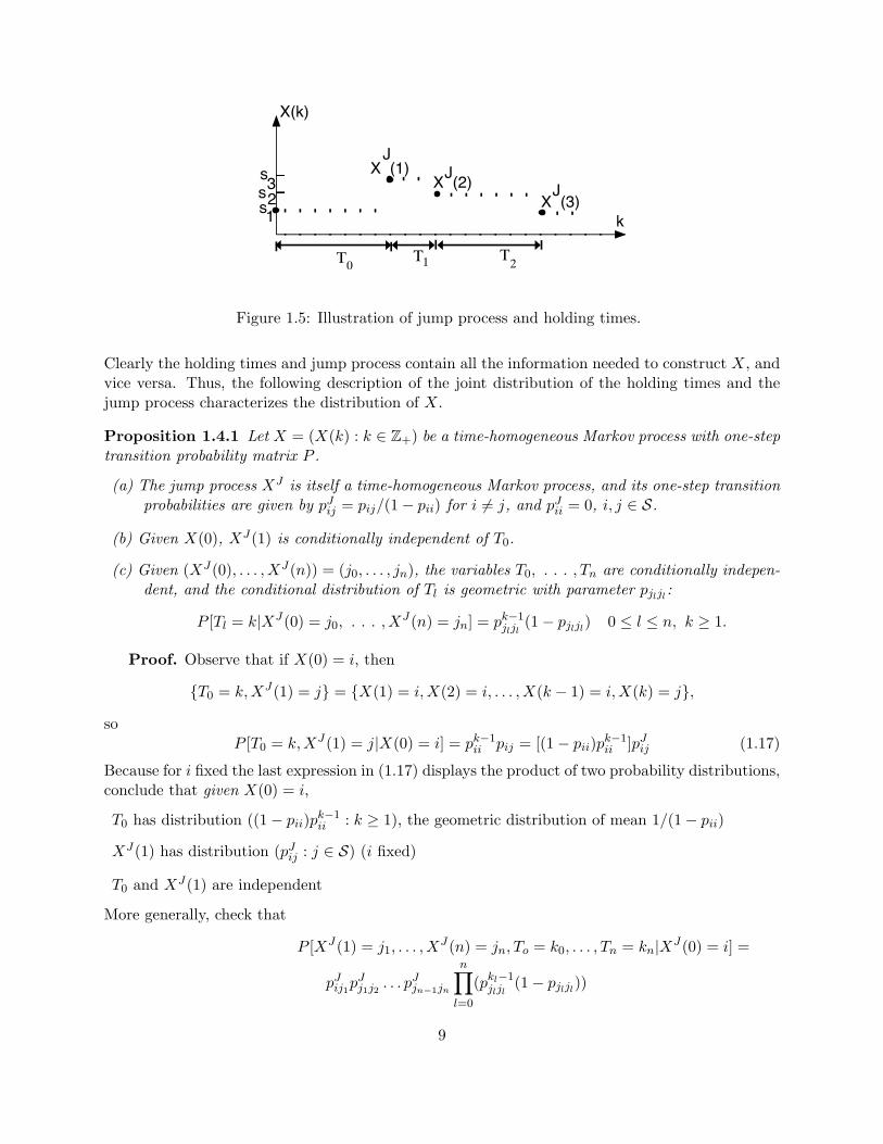
Let (Xk : k ∈ Z+) be a time-homogeneous Markov process with one-step transition probabilitymatrix P . Let Tk denote the time that elapses between the kth and k + 1th jumps of X, and letXJ(k) denote the state after k jumps. See Fig. 1.5 for illustration. More precisely, the holdingtimes are defined by

T0 = mint ≥ 0 : X(t) 6= X(0) (1.14)Tk = mint ≥ 0 : X(T0 + . . . + Tk−1 + t) 6= X(T0 + . . . + Tk−1) (1.15)

and the jump process XJ = (XJ(k) : k ≥ 0) is defined by

XJ(0) = X(0) and XJ(k) = X(T0 + . . . + Tk−1) (1.16)

8

! !0 1 2!

X (3)

X(k)

J

k

X (1) X (2) J

Jsss123

Figure 1.5: Illustration of jump process and holding times.

Clearly the holding times and jump process contain all the information needed to construct X, andvice versa. Thus, the following description of the joint distribution of the holding times and thejump process characterizes the distribution of X.

Proposition 1.4.1 Let X = (X(k) : k ∈ Z+) be a time-homogeneous Markov process with one-steptransition probability matrix P .

(a) The jump process XJ is itself a time-homogeneous Markov process, and its one-step transitionprobabilities are given by pJ

ij = pij/(1− pii) for i 6= j, and pJii = 0, i, j ∈ S.

(b) Given X(0), XJ(1) is conditionally independent of T0.

(c) Given (XJ(0), . . . , XJ(n)) = (j0, . . . , jn), the variables T0, . . . , Tn are conditionally indepen-dent, and the conditional distribution of Tl is geometric with parameter pjljl

:

P [Tl = k|XJ(0) = j0, . . . , XJ(n) = jn] = pk−1jljl

(1− pjljl) 0 ≤ l ≤ n, k ≥ 1.

Proof. Observe that if X(0) = i, then

T0 = k, XJ(1) = j = X(1) = i, X(2) = i, . . . , X(k − 1) = i, X(k) = j,

soP [T0 = k, XJ(1) = j|X(0) = i] = pk−1

ii pij = [(1− pii)pk−1ii ]pJ

ij (1.17)

Because for i fixed the last expression in (1.17) displays the product of two probability distributions,conclude that given X(0) = i,

T0 has distribution ((1− pii)pk−1ii : k ≥ 1), the geometric distribution of mean 1/(1− pii)

XJ(1) has distribution (pJij : j ∈ S) (i fixed)

T0 and XJ(1) are independent

More generally, check that

P [XJ(1) = j1, . . . , XJ(n) = jn, To = k0, . . . , Tn = kn|XJ(0) = i] =

pJij1p

Jj1j2 . . . pJ

jn−1jn

n∏l=0

(pkl−1jljl

(1− pjljl))

9

X(t)

t

(h)X (1) X (2) (h)X (3) (h)

sss123

Figure 1.6: Illustration of sampling of a pure-jump function

This establishes the proposition.

Next we consider the space-time structure of time-homogeneous continuous-time pure-jumpMarkov processes. Essentially the only difference between the discrete- and continuous-time Markovprocesses is that the holding times for the continuous-time processes are exponentially distributedrather than geometrically distributed. Indeed, define the holding times Tk, k ≥ 0 and the jumpprocess XJ using (1.14)-(1.16) as before.

Proposition 1.4.2 Let X = (X(t) : t ∈ R+) be a time-homogeneous, pure-jump Markov processwith generator matrix Q. Then

(a) The jump process XJ is a discrete-time, time-homogeneous Markov process, and its one-steptransition probabilities are given by

pJij =

−qij/qii for i 6= j0 for i = j

(1.18)

(b) Given X(0), XJ(1) is conditionally independent of T0.

(c) Given XJ(0) = j0, . . . , XJ(n) = jn, the variables T0, . . . , Tn are conditionally independent,and the conditional distribution of Tl is exponential with parameter −qjljl

:

P [Tl ≥ c|XJ(0) = j0, . . . , XJ(n) = jn] = exp(cqjljl) 0 ≤ l ≤ n.

Proof. Fix h > 0 and define the “sampled” process X(h) by X(h)(k) = X(hk) for k ≥ 0. SeeFig. 1.6. Then X(h) is a discrete time Markov process with one-step transition probabilities pij(h)(the transition probabilities for the original process for an interval of length h). Let (T (h)

k : k ≥ 0)denote the sequence of holding times and (XJ,h(k) : k ≥ 0) the jump process for the process X(h).

The assumption that with probability one the sample paths of X are pure-jump functions,implies that with probability one:

limh→0

(XJ,h(0), XJ,h(1), . . . , XJ,h(n), hT(h)0 , hT

(h)1 , . . . , hT (h)

n ) =

(XJ(0), XJ(1), . . . , XJ(n), T0, T1, . . . , Tn) (1.19)

10

1 2 30

1

1 2

2 3

3

0

4µ

!

µµµ

!!!

Figure 1.7: Transition rate diagram of a birth-death process

Since convergence with probability one implies convergence in distribution, the goal of identifyingthe distribution of the random vector on the righthand side of (1.19) can be accomplished byidentifying the limit of the distribution of the vector on the left.

First, the limiting distribution of the process XJ,h is identified. Since X(h) has one-step transi-tion probabilities pij(h), the formula for the jump process probabilities for discrete-time processes(see Proposition 1.4.1, part a) yields that the one step transition probabilities pJ,h

ij for X(J,h) aregiven by

pJ,hij =

pij(h)1− pii(h)

=pij(h)/h

(1− pii(h))/h→ qij

−qiias h → 0 (1.20)

for i 6= j, where the limit indicated in (1.20) follows from the definition (1.9) of the generator matrixQ. Thus, the limiting distribution of XJ,h is that of a Markov process with one-step transitionprobabilities given by (1.18), establishing part (a) of the proposition. The conditional independenceproperties stated in (b) and (c) of the proposition follow in the limit from the correspondingproperties for the jump process XJ,h guaranteed by Proposition 1.4.1. Finally, since log(1 + θ) =θ + o(θ) by Taylor’s formula, we have for all c ≥ 0 that

P [hT(h)l > c|XJ,h(0) = j0, . . . , X

J,h = jn] = (pjljl(h))bc/hc

= exp(bc/hc log(pjljl(h)))

= exp(bc/hc(qjljlh + o(h)))

→ exp(qjljlc) as h → 0

which establishes the remaining part of (c), and the proposition is proved.

Birth-Death Processes A useful class of countable state Markov processes is the set ofbirth-death processes. A (continuous time) birth-death process with parameters (λ0, λ2, . . .) and(µ1, µ2, . . .) (also set λ−1 = µ0 = 0) is a pure-jump Markov process with state space S = Z+ andgenerator matrix Q defined by qkk+1 = λk, qkk = −(µk +λk), and qkk−1 = µk for k ≥ 0, and qij = 0if |i− j| ≥ 2. The transition rate diagram is shown in Fig. (1.7). The space-time structure of sucha process is as follows. Given the process is in state k at time t, the next state visited is k + 1 withprobability λk/(λk + µk) and k − 1 with probability µk/(λk + µk). The holding time of state k isexponential with parameter λk + µk.

11

The space-time structure just described can be used to show that the limit in (1.9) is uniformin i for j fixed, so that the Kolmogorov forward equations are satisfied. These equations are:

∂πk(t)∂t

= λk−1πk−1(t)− (λ + µ)πk(t) + µk+1πk+1(t) (1.21)

1.5 Poisson Processes

A Poisson process with rate λ is a birth-death process N = (N(t) : t ≥ 0) with initial distributionP [N(0) = 0] = 1, birth rates λk = λ for all k and death rates µk = 0 for all k. The space-timestructure is particularly simple. The jump process NJ is deterministic and is given by NJ(k) = k.Therefore the holding times are not only conditionally independent given NJ , they are independentand each is exponentially distributed with parameter λ.

Let us calculate πj(t) = P [N(t) = j]. The Kolmogorov forward equation for k = 0 is ∂π0/∂t =−λπ0, from which we deduce that π0(t) = exp(−λt). Next the equation for π1 is ∂π1/∂t =λ exp(−λt)−λπ1(t) which can be solved to yield π1(t) = (λt) exp(−λt). Continuing by induction onk, verify that πk(t) = (λt)k exp(−λt)/k!, so that N(t) is a Poisson random variable with parameterk.

It is instructive to solve the Kolmogorov equations by another method, namely the z-transformmethod, since it works for some more complex Markov processes as well. For convenience, setπ−1(t) = 0 for all t. Then the Kolmogorov equations for π become ∂πk

∂t = λπk−1−λπk. Multiplyingeach side of this equation by zk, summing over k, and interchanging the order of summationand differentiation, yields that the z transform P ∗(z, t) of π(t) satisfies ∂P ∗(z,t)

∂t = (λz − λ)P ∗(z, t).Solving this with the initial condition P ∗(z, 0) = 1 yields that P ∗(z, t) = exp((λz−λ)t). Expandingexp(λzt) into powers of z identifies (λt)k exp(−λt)/k! as the coefficient of zn in P ∗(z, t).

In general, for i fixed, pij(t) is determined by the same equations but with the initial distributionpij(0) = Ii=j. The resulting solution is pij(t) = πj−i(t) for j ≥ i and pij(t) = 0 otherwise. Thusfor t0 < t1 < . . . < td = s < t,

P [N(t)−N(s) = l|N(t0) = i0, . . . , N(td−1) = id−1, N(s) = i]= P [N(t) = i + l|N(s) = i]= [λ(t− s)]l exp(−λ(t− s))/l!

Conclude that N(t)−N(s) is a Poisson random variable with mean λ(t− s). Furthermore, N(t)−N(s) is independent of (N(u) : u ≤ s), which implies that the increments N(t1) −N(t0), N(t2) −N(t1), N(t3)−N(t2), . . . are mutually independent whenever 0 ≤ t0 < t1 < . . ..

Turning to another characterization, fix T > 0 and λ > 0, let U1, U2, . . . be uniformly distributedon the interval [0, T ], and let K be a Poisson random variable with mean λT . Finally, define therandom process (N(t) : 0 ≤ t ≤ T ) by

N(t) =K∑

i=1

It≥Ui. (1.22)

That is, for 0 ≤ t ≤ T , N(t) is the number of the first K uniform random variables located in[0, t]. We claim that N has the same distribution as a Poisson random process N with parameter λ,restricted to the interval [0, T ]. To verify this claim, it suffices to check that the increments of the two

12

processes have the same joint distribution. To that end, fix 0 = t0 < t1 . . . < td = T and nonnegativeintegers k1, . . . , kd. Define the event A = N(t1) − N(t0) = k1, . . . , N(td) − N(td−1) = kd, anddefine the event A in the same way, but with N replaced by N . It is to be shown that P [A] = P [A].

The independence of the increments of N and the Poisson distribution of each increment of Nimplies that

P [A] =d∏

i=1

(λ(ti − ti−1))ki exp(−λ(ti − ti−1))/ki!. (1.23)

On the other hand, the event A is equivalent to the condition that K = k, where k = k1 + . . . + kd,and that furthermore the k random variables U1, . . . , Uk are distributed appropriately across the dsubintervals. Let pi = (ti − ti−1)/T denote the relative length of the ith subinterval [ti−1, ti]. Theprobability that the first k1 points U1, . . . , Uk1 fall in the first interval [t0, t1], the next k2 pointsfall in the next interval, and so on, is pk1

1 pk22 . . . pkd

d . However, there are(

kk1 ... kd

)= k!

k1!...kd! equallylikely ways to assign the variables U1, . . . , Uk to the intervals with ki variables in the ith intervalfor all i, so

P [A] = P [K = k](

k

k1 . . . kd

)pk11 . . . pkd

d , (1.24)

Some rearrangement yields that P [A] = P [A], as was to be shown. Therefore, N and N restrictedto the time interval [0, T ] have the same distribution.

The above discussion provides some useful characterizations of a Poisson process, which aresummarized in the following proposition. Suppose that X = (X(t) : t ≥ 0) has pure-jump samplepaths with probability one, suppose P [X(0) = 0] = 1, and suppose λ > 0.

Proposition 1.5.1 The following four are equivalent:

(i) X is a Poisson process with rate λ.

(ii) The jumps of X are all size one, and the holding times are independent, exponentially dis-tributed with parameter λ.

(iii) Whenever 0 ≤ t0 < t1 . . . < tn, the increments X(t1) − X(t0), . . . , X(tn) − X(tn−1)are independent random variables, and whenever 0 ≤ s < t, the increment X(t) −X(s) is aPoisson random variable with mean λ(t− s).

(iv) Whenever 0 ≤ s < t, the increment X(t) − X(s) is a Poisson random variable with meanλ(t − s), and given X(t) −X(s) = n, the jumps of X in [s, t] are height one and the vectorof their locations is uniformly distributed over the set τ ∈ Rn

+ : s < τ1 < . . . < τn < t.

The fourth characterization of 1.5.1 can be readily extended to define Poisson point processeson any set with a suitable positive measure giving the mean number of points within subsets. Forexample, a Poisson point process on Rd with intensity λ is specified by the following two conditions.First, for any subset A of Rd with finite volume, the distribution of the number of points in theset is Poisson with mean λ · V olume(A). Second, given that the number of points in such a setA is n, the locations of the points within A are distributed according to n mutually independentrandom variables, each uniformly distributed over A. As a sample calculation, take d = 2 andconsider the distance R of the closest point of the Poisson point process to the origin. Since the

13

number of points falling within a circle of radius r has the Poisson distribution with mean πr2, thedistribution function of R is given by

P [R ≤ r] = 1-P[no points of the process in circle of radius r] = 1− exp(λπr2).

1.6 Renewal Theory

Renewal theory describes convergence to statistical equilibrium for systems involving sequences ofintervals of random duration. It also helps describe what is meant by the state of a random systemat a typical time, or as viewed by a typical customer. We begin by examining Poisson processesand an illustration of the dependence of an average on the choice of sampling distribution.

Consider a two-sided Poisson process (N(t) : t ∈ R) with parameter λ, which by definitionmeans that N(0) = 0, N is right-continuous, the increment N(t + s) − N(t) is a Poisson randomvariable with mean λ for any s > 0 and t, and the increments of N are independent. Fix a time t.With probability one, t is strictly in between two jump times of N . The time between t and the firstjump after time t is exponentially distributed, with mean 1/λ. Similarly, the time between the lastjump before time t and t is also exponentially distributed with mean 1/λ. (In fact, these two timesare independent.) Thus, the mean of the length of the interval between the jumps surrounding tis 2/λ. In contrast, the Poisson process is built up from exponential random variables with mean1/λ. That the two means are distinct is known as the “Poisson paradox.”

Perhaps an analogy can help explain the Poisson paradox. Observe that the average populationof a country on earth is about 6 × 109/200 = 30 million people. On the other hand, if a personis chosen at random from among all people on earth, the mean number of people in the samecountry as that person is greater than 240 million people. Indeed, the population of China is about1.2× 109, so that about one of five people live in China. Thus, the mean number of people in thesame country as a randomly selected person is at least 1.2×109/5=240 million people. The secondaverage is much larger than the first, because sampling a country by choosing a person at randomskews the distribution of size towards larger countries in direct proportion to the populations of thecountries. In the same way, the sampled lifetime of a Poisson process is greater than the typicallifetimes used to generate the process.

A generalization of the Poisson process is a counting process in which the times between arrivalsare independent and identically distributed, but not necessarily exponentially distributed. Forslightly more generality, the time until the first arrival is allowed to have a distribution differentfrom the lengths of times between arrivals, as follows.

Suppose F and G are distribution functions of nonnegative random variables, and to avoidtrivialities, suppose that F (0) < 1. Let T1, T2, . . . be independent, such that T1 has distributionfunction G and Tk has distribution function F for k ≥ 2. The time of the nth arrival is τ(n) =T1 + T2 + . . . + Tn and the number of arrivals up to time t is α(t) = maxn : τ(n) ≤ t. Theresidual lifetime at a fixed time t is defined to be γt = τ(α(t) + 1)− t and the sampled lifetime at afixed time t is Lt = Tα(t)+1, as pictured in Figure 1.8. 1 Renewal theory, the focus of this section,describes the limits of the residual lifetime and sampled lifetime distributions for such processes.

This section concludes with a presentation of the renewal equation, which plays a key role inrenewal theory. To write the equation in general form, the definition of convolution of two measureson the real line, given next, is needed. Let F1 and F2 be two distribution functions, corresponding

1Note that if one or more arrivals occur at a time t, then γt and Lt are both equal to the next nonzero lifetime.

14

t

Lt! t

Figure 1.8: Sampled lifetime and forward lifetime

to two positive measures on the real line. The convolution of the two measures is again a measure,such that its distribution function is F1 ∗ F2, defined by the Riemann-Stieltjes integral

F1 ∗ F2(x) =∫ ∞

−∞F1(x− y)F2(dy)

If X1 and X2 are independent random variables, if X1 has distribution function F1, and if X2 hasdistribution function F2, then X1 + X2 has distribution function F1 ∗ F2. It is clear from this thatconvolution is commutative (F ∗ G = G ∗ F ) and associative ((F ∗ G) ∗H = F ∗ (G ∗H)). If F1

has density function f1 and F2 has density function F2, then F1 ∗ F2 has density function f1 ∗ f2,defined as the usual convolution of functions on R:

f1 ∗ f2(x) =∫ ∞

−∞f1(x− y)f2(y)dy

Similarly, if F1 has a discrete mass function f1 on Z and F2 has discrete mass function f2 on Z,then F1 ∗ F2 has discrete mass function f1 ∗ f2 defined as the usual convolution of functions on Z:

f1 ∗ f2(n) =∞∑

k=−∞f1(n− k)f2(k).

Define the cumulative mean renewal function H by H(t) = E[α(t)]. Function H can be viewedas the cumulative distribution function for the renewal measure, which is the measure on R+ suchthat the measure of an interval is the mean number of arrivals in the interval. In particular, for0 ≤ s ≤ t, H(t) − H(s) is the mean number of arrivals in the interval (s, t]. The function Hdetermines much about the renewal variables–in particular the joint distribution of (Lt, γt) can beexpressed in terms of H and the CDFs F and G. For example, if t ≥ u > 0, then

P [Lt ≤ u] =∫ t

t−uP [a renewal occurs in [s, s + ds] with lifetime ∈ [t− s, u]]

=∫ t

t−u(F (u)− F (t− s))dH(s). (1.25)

Observe that the function H can be expressed as

H(t) =∞∑

n=1

Un(t) (1.26)

where Un is the probability distribution function of T1 + · · ·+Tn. From (1.26) and the facts U1 = Gand Un = F ∗ Un−1 for n ≥ 2, the renewal equation follows:

H = G + F ∗H

15

1.6.1 Renewal Theory in Continuous Time

The distribution function F is said to be lattice type if, for some a > 0, the distribution is con-centrated on the set of integer multiples of a. Otherwise F is said to be nonlattice type. In thissubsection F is assumed to be nonlattice type, while the next subsection touches on discrete-timerenewal theory, addressing the situations when F is lattice type. If F and G have densities, then Hhas a density and the renewal equation can be written as h = g+f ∗h. Many convergence questionsabout renewal processes, and also about Markov processes, can be settled by the following theorem(for a proof, see [1, 18]).

Proposition 1.6.1 (Blackwell’s Renewal Theorem in continuous time) Suppose F is a nonlatticedistribution. Then for fixed h > 0,

limt→∞

(H(t + h)−H(t))/h = 1/m1,

where mk is the kth moment of F .

The renewal theorem can be used to show that if the distribution F is nonlattice, then

limt→∞

P [Lt ≤ u, γt ≤ s] = FLγ(u, s)

where

FLγ(u, s) =1

m1

∫ s∧u

0(F (u)− F (y))dy u, s ∈ R+ (1.27)

For example, to identify limt→∞ P [Lt ≤ u] one can start with (1.25). Roughly speaking, the renewaltheorem tells us that in the limit, we can replace dH(s) in (1.25) by ds

m1. This can be justified by

transforming the representation (1.25) by a change of variables (letting x = t − s for t fixed) andan integration by parts, before applying the renewal theorem, as follows

P [Lt ≤ u] = −∫ u

0(F (u)− F (x))dH(t− x)

=∫ u

0(H(t)−H(t− x))dF (x)

→∫ u

0

x

m1dF (x) =

1m1

∫ u

0(F (u)− F (y))dy

The following properties of the joint distribution of (L, γ) under FLγ are usually much easier towork with than the expression (1.27):

Moments: E[Lk] = mk+1/m1 and E[γk] = mk+1/((k + 1)m1),

Density of γ: γ has density fγ(s) = (1− F (s))/m1,

Joint density: If F has density f , then (L, γ) has density

fL,γ(u, s) =

f(u)/m1 if 0 ≤ s ≤ u0 else

Equivalently, L has density fL(u) = uf(u)/m1 and given L = u, γ is uniformly distributedover the interval [0, u].

16

Laplace transforms: F ∗γ (s) = (1− F ∗(s))/(sm1) and F ∗

L(s) = −(dF ∗(s)/ds)/m1.

The fact that the stationary sampled lifetime density, fL(u), is proportional to uf(u), makessense according to the intuition gleaned from the countries example. The lifetimes here play the roleof countries in that example, and sampling by a particular time (analogous to selecting a countryby first selecting an individual) results in a factor u proportional to the size of the lifetime.

1.6.2 Renewal Theory in Discrete Time

Suppose that the variables T1, T2, . . . are integer valued. The process α(t) need only be consideredfor integer values of t. The renewal equation can be written as h = g + f ∗ h. where h(n) isthe expected number of renewals that occur at time n, and f and g are the probability massfunctions corresponding to F and G. The z-transform of h is readily found to be given by H(z) =G(z)/(1− F (z)).

Recall that the greatest common divisor, GCD, of a set of positive integers is the largest integerthat evenly divides all the integers in the set. For example, GCD4, 6, 12 = 2.

Proposition 1.6.2 (Blackwell’s Renewal Theorem in discrete time) Suppose GCDk ≥ 1 : f(k) >0 = 1. Then limn→∞ h(n) = 1/m1, where mk is the kth moment of F .

The proposition can be used to prove the following fact. If GCDk ≥ 1 : f(k) > 0 = 1, then(Ln, γn) converges in distribution as n →∞, and under the limiting distribution

P [L = l] = lfl/m1 and P [γ = i|L = l] = 1/l 1 ≤ i ≤ l,

P [γ = i] =1− F (i− 1)

m1i ≥ 1

andE[Lk] = mk+1/m1 and E[γ] = ((m2/2m1)) + 0.5.

Note that if a renewal occurs at time t, then by definition γt is the time between t and the firstrenewal after time t. An alternative definition would take γt equal to zero in such a case. Underthe alternative definition, E[γ] = ((m2/2m1)) − 0.5. In fact, this is the same as the mean of thebackwards residual arrival time for the original definition. In contrast, in continuous time, both theforward and backward residual lifetimes have mean m2/2m1.

1.7 Classification and Convergence of Discrete State Markov Pro-cesses

1.7.1 Examples with finite state space

Recall that a probability distribution π on S is an equilibrium probability distribution for a time-homogeneous Markov process X if π = πH(t) for all t. We shall see in this section that undercertain natural conditions, the existence of an equilibrium probability distribution is related towhether the distribution of X(t) converges as t → ∞. Existence of an equilibrium distribution isalso connected to the mean time needed for X to return to its starting state. To motivate theconditions that will be imposed, we begin by considering four examples of finite state processes.

17

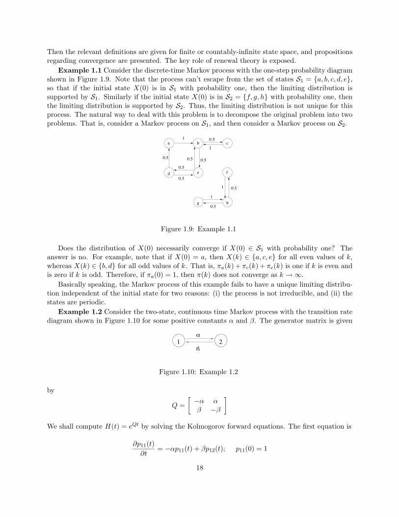
Then the relevant definitions are given for finite or countably-infinite state space, and propositionsregarding convergence are presented. The key role of renewal theory is exposed.

Example 1.1 Consider the discrete-time Markov process with the one-step probability diagramshown in Figure 1.9. Note that the process can’t escape from the set of states S1 = a, b, c, d, e,so that if the initial state X(0) is in S1 with probability one, then the limiting distribution issupported by S1. Similarly if the initial state X(0) is in S2 = f, g, h with probability one, thenthe limiting distribution is supported by S2. Thus, the limiting distribution is not unique for thisprocess. The natural way to deal with this problem is to decompose the original problem into twoproblems. That is, consider a Markov process on S1, and then consider a Markov process on S2.

0.5

1

0.50.5

0.5

0.5

1

1 0.5

0.5

b c

d e f

g h

a

0.5

1

Figure 1.9: Example 1.1

Does the distribution of X(0) necessarily converge if X(0) ∈ S1 with probability one? Theanswer is no. For example, note that if X(0) = a, then X(k) ∈ a, c, e for all even values of k,whereas X(k) ∈ b, d for all odd values of k. That is, πa(k) + πc(k) + πe(k) is one if k is even andis zero if k is odd. Therefore, if πa(0) = 1, then π(k) does not converge as k →∞.

Basically speaking, the Markov process of this example fails to have a unique limiting distribu-tion independent of the initial state for two reasons: (i) the process is not irreducible, and (ii) thestates are periodic.

Example 1.2 Consider the two-state, continuous time Markov process with the transition ratediagram shown in Figure 1.10 for some positive constants α and β. The generator matrix is given

!

"1 2


by

Q =[−α αβ −β

]We shall compute H(t) = eQt by solving the Kolmogorov forward equations. The first equation is

∂p11(t)∂t

= −αp11(t) + βp12(t); p11(0) = 1

18

But p12(t) = 1− p11(t), so

∂p11(t)∂t

= −(α + β)p11(t) + β; p11(0) = 1

By differentiation we check that this equation has the solution

p11(t) = e−(α+β)t +∫ t

0e−(α+β)(t−s)βds

=β

α + β(1− e−(α+β)t).

Using the fact p12(t) = 1 − p11(t) yields p12(t). The second row of H(t) can be found similarly,yielding

H(t) =

[β

α+βα

α+ββ

α+βα

α+β

]+ e−(α+β)t

[α

α+β − αα+β

− βα+β

βα+β

]Note that H(0) = I as required, and that

limt→∞

H(t) =

[β

α+βα

α+ββ

α+βα

α+β

]

Thus, for any initial distribution π(0),

limt→∞

π(t) = limt→∞

π(0)H(t) = (β

α + β,

α

α + β).

The rate of convergence is exponential, with rate parameter α+β, which happens to be the nonzeroeigenvalue of Q. Note that the limiting distribution is the unique probability distribution satisfyingπQ = 0. The periodicity problem of Example 1.1 does not arise for continuous-time processes.

Example 1.3 Consider the continuous-time Markov process with the transition rate diagramin Figure 1.11. The Q matrix is the block-diagonal matrix given by

!

"1 2

!

"3 4


Q =

−α α 0 0β −β 0 00 0 −α α0 0 β −β

This process is not irreducible, but rather the transition rate diagram can be decomposed into twoparts, each equivalent to the diagram for Example 1.1. The equilibrium probability distributionsare the probability distributions of the form π = (λ β

α+β , λ αα+β , (1− λ) β

α+β , (1− λ) αα+β ), where λ is

the probability placed on the subset 1, 2.

19

1 2

3

1

11


Example 1.4 Consider the discrete-time Markov process with the transition probability dia-gram in Figure 1.12. The one-step transition probability matrix P is given by

P =

0 1 00 0 11 0 0

Solving the equation π = πP we find there is a unique equilibrium probability vector, namelyπ = (1

3 , 13 , 1

3). On the other hand, if π(0) = (1, 0, 0), then

π(k) = π(0)P k =

(1, 0, 0) if k ≡ 0 mod 3(0, 1, 0) if k ≡ 1 mod 3(0, 0, 1) if k ≡ 2 mod 3

Therefore, π(k) does not converge as k →∞.Let X be a discrete-time, or pure-jump continuous-time, Markov process on the countable state

space S. Suppose X is time-homogeneous. The process is said to be irreducible if for all i, j ∈ S,there exists s > 0 so that pij(s) > 0.

1.7.2 Discrete Time

Clearly a probability distribution π is an equilibrium probability distribution for a discrete-timetime-homogeneous Markov process X if and only if π = πP . The period of a state i is definedto be GCDk ≥ 0 : pii(k) > 0. The set k ≥ 0 : pii(k) > 0 is closed under addition, whichby elementary algebra 2 implies that the set contains all sufficiently large integer multiples of theperiod. The Markov process is called aperiodic if the period of all the states is one.

Proposition 1.7.1 If X is irreducible, all states have the same period.

Proof. Let i and j be two states. By irreducibility, there are integers k1 and k2 so that pij(k1) > 0and pji(k2) > 0. For any integer n, pii(n + k1 + k2) ≥ pij(k1)pjj(n)pji(k2), so the set k ≥ 0 :pii(k) > 0 contains the set k ≥ 0 : pjj(k) > 0 translated up by k1 + k2. Thus the period of i isless than or equal to the period of j. Since i and j were arbitrary states, the proposition follows.

For a fixed state i, define τi = mink ≥ 1 : X(k) = i, where we adopt the conventionthat the minimum of an empty set of numbers is +∞. Let Mi = E[τi|X(0) = i]. If P [τi <+∞|X(0) = i] < 1, then state i is called transient (and by convention, Mi = +∞). OtherwiseP[τi < +∞|X(0) = i] = 1, and i is then said to be positive − recurrent if Mi < +∞ and to benull − recurrent if Mi = +∞.

2see Euclidean algorithm, Chinese remainder theorem, Bezout theorem

20

Proposition 1.7.2 Suppose X is irreducible and aperiodic.

(a) All states are transient, or all are positive-recurrent, or all are null-recurrent.

(b) For any initial distribution π(0), limt→∞ πi(t) = 1/Mi, with the understanding that the limitis zero if Mi = +∞.

(c) An equilibrium probability distribution π exists if and only if all states are positive-recurrent.

(d) If it exists, the equilibrium probability distribution π is given by πi = 1/Mi. (In particular, ifit exists, the equilibrium probability distribution is unique).

Proof. (a) Suppose state i is recurrent. Given X(0) = i, after leaving i the process returns tostate i at time τi. The process during the time interval 0, . . . , τi is the first excursion of X fromstate 0. From time τi onward, the process behaves just as it did initially. Thus there is a secondexcursion from i, third excursion from i, and so on. Let Tk for k ≥ 1 denote the length of the kthexcursion. Then the Tk’s are independent, and each has the same distribution as T1 = τi. Let j beanother state and let ε denote the probability that X visits state j during one excursion from i.Since X is irreducible, ε > 0. The excursions are independent, so state j is visited during the kthexcursion with probability ε, independently of whether j was visited in earlier excursions. Thus, thenumber of excursions needed until state j is reached has the geometric distribution with parameterε, which has mean 1/ε. In particular, state j is eventually visited with probability one. After jis visited the process eventually returns to state i, and then within an average of 1/ε additionalexcursions, it will return to state j again. Thus, state j is also recurrent. Hence, if one state isrecurrent, all states are recurrent.

The same argument shows that if i is positive-recurrent, then j is positive-recurrent. GivenX(0) = i, the mean time needed for the process to visit j and then return to i is Mi/ε, since onaverage 1/ε excursions of mean length Mi are needed. Thus, the mean time to hit j starting fromi, and the mean time to hit i starting from j, are both finite. Thus, j is positive-recurrent. Hence,if one state is positive-recurrent, all states are positive-recurrent.

(b) Part (b) of the proposition follows immediately from the renewal theorem for discrete time.The first lifetime for the renewal process is the time needed to first reach state i, and the subsequentrenewal times are the lengths of the excursions from state i. The probability πi(t) is the probabilitythat there is a renewal event at time t, which by the renewal theorem converges to 1/Mi.

(c) Suppose all states are positive-recurrent. By the law of large numbers, for any state j, thelong run fraction of time the process is in state j is 1/Mj with probability one. Similarly, for anystates i and j, the long run fraction of time the process is in state j is γij/Mi, where γij is themean number of visits to j in an excursion from i. Therefore 1/Mj = γij/Mi. This implies that∑

i 1/Mi = 1. That is, π defined by πi = 1/Mi is a probability distribution. The convergence foreach i separately given in part (b), together with the fact that π is a probability distribution, implythat

∑i |πi(t) − πi| → 0. Thus, taking s to infinity in the equation π(s)H(t) = π(s + t) yields

πH(t) = π, so that π is an equilibrium probability distribution.Conversely, if there is an equilibrium probability distribution π, consider running the process

with initial state π. Then π(t) = π for all t. So by part (b), for any state i, πi = 1/Mi. Taking astate i such that πi > 0, it follows that Mi < ∞. So state i is positive-recurrent. By part (a), allstates are positive-recurrent.

(d) Part (d) was proved in the course of proving part (c).

21

We conclude this section by describing a technique to establish a rate of convergence to theequilibrium distribution for finite-state Markov processes. Define δ(P ) for a one-step transitionprobability matrix P by

δ(P ) = mini,k

∑j

pij ∧ pkj ,

where a∧ b = mina, b. The number δ(P ) is known as Dobrushin’s coefficient of ergodicity. Sincea + b− 2(a ∧ b) = |a− b| for a, b ≥ 0, we also have

1− 2δ(P ) = mini,k

∑j

|pij − pkj |.

Let ‖µ‖ for a vector µ denote the L1 norm: ‖µ‖ =∑

i |µi|.

Proposition 1.7.3 For any probability vectors π and σ, ‖πP −σP‖ ≤ (1−δ(P ))‖π−σ‖. Further-more, if δ(P ) > 0 then there is a unique equilibrium distribution π∞, and for any other probabilitydistribution π on S, ‖πP l − π∞‖ ≤ 2(1− δ(P ))l.

Proof. Let πi = πi − πi ∧ σi and σi = σi − πi ∧ σi. Clearly ‖π − σ‖ = ‖π − σ‖ = 2‖π‖ = 2‖σ‖.Furthermore,

‖πP − σP‖ = ‖πP − σP‖=

∑j

‖∑

i

πiPij −∑

k

σkPkj‖

= (1/‖π‖)∑

j

|∑i,k

πiσk(Pij − Pkj)|

≤ (1/‖π‖)∑i,k

πiσk

∑j

|Pij − Pkj |

≤ ‖π‖(2− 2δ(P )) = ‖π − σ‖(1− δ(P )),

which proves the first part of the proposition. Iterating the inequality just proved yields that

‖πP l − σP l‖ ≤ (1− δ)l‖π − σ‖ ≤ 2(1− δ)l. (1.28)

This inequality for σ = πPn yields that ‖πP l − πP l+n‖ ≤ 2(1 − δ)l. Thus the sequence πP l is aCauchy sequence and has a limit π∞, and π∞P = π∞. Finally, taking σ in (1.28) equal to π∞

yields the last part of the proposition.

Proposition 1.7.3 typically does not yield the exact asymptotic rate that ‖πl − π∞‖ tends tozero. The asymptotic behavior can be investigated by computing (I − zP )−1, and then matchingpowers of z in the identity (I − zP )−1 =

∑∞n=0 znPn.

1.7.3 Continuous Time

Define, for i ∈ S, τ oi = mint > 0 : X(t) 6= i, and τi = mint > τ o

i : X(t) = i. Thus, ifX(0) = i, τi is the first time the process returns to state i, with the exception that τi = +∞if the process never returns to state i. The following definitions are the same as when X is adiscrete-time process. Let Mi = E[τi|X(0) = i]. If P [τi < +∞] < 1, then state i is called transient.

22

Otherwise P [τi < +∞] = 1, and i is then said to be positive − recurrent if Mi < +∞ and to benull − recurrent if Mi = +∞.

The following propositions are analogous to those for discrete-time Markov processes. Proofscan be found in [1, 32].

Proposition 1.7.4 Suppose X is irreducible.

(a) All states are transient, or all are positive-recurrent, or all are null-recurrent.

(b) For any initial distribution π(0), limt→+∞ πi(t) = 1/(−qiiMi), with the understanding that thelimit is zero if Mi = +∞.

Proposition 1.7.5 Suppose X is irreducible and nonexplosive.

(a) A probability distribution π is an equilibrium distribution if and only if πQ = 0.

(b) An equilibrium probability distribution exists if and only if all states are positive-recurrent.

(c) If all states are positive-recurrent, the equilibrium probability distribution is given by πi =1/(−qiiMi). (In particular, if it exists, the equilibrium probability distribution is unique).

Once again, the renewal theorem leads to an understanding of the convergence result of part(b) in Proposition 1.7.4. Let Tk denote the amount of time between the kth and k + 1th visits tostate i. Then the variables Tk : k ≥ 0 are independent and identically distributed, and hence thesequence of visiting times is a renewal sequence. Let H(t) denote the expected number of visits tostate i during the interval [0, t], so that H is the cumulative mean renewal function for the sequenceT1, T2, . . .. As above, note that Mi = E[Tk].

The renewal theorem is applied next to show that

limt→∞

P [X(t) = i] = 1/(−qiiMi). (1.29)

Indeed, note that the definition of H, the fact that holding times for state i are exponentiallydistributed with parameter qii, integration by parts, a change of variable, and the renewal theorem,imply that

P [X(t) = i] = P [X(t) = i, T1 > t] +∫ t

0P [X(t) = i, (last renewal before t) ∈ ds]

= P [X(0) = i] exp(qiit) +∫ t

0exp(qii(t− s))dH(s)

= P [X(0) = i] exp(qiit) +∫ t

0exp(qii(t− s))(−qii)H(t)−H(s)ds

= P [X(0) = i] exp(qiit) +∫ t

0exp(qiiu)(−qii)H(t)−H(t− u)du

→∫ ∞

0exp(qiiu)(−qii)(u/Mi)du = 1/(−qiiMi).

This establishes (1.29).

23

An immediate consequence of (1.29) is that if there is an equilibrium distribution π, then theMarkov process is positive recurrent and the equilibrium distribution is given by

πi = 1/(−qiiMi). (1.30)

Conversely, if the process is positive recurrent, then there is an equilibrium probability distributionand it is given by (1.30).

Part (a) of Proposition 1.7.5 is suggested by the Kolmogorov forward equation ∂π(t)/∂t =π(t)Q. The assumption that X be nonexplosive is needed (per homework problem), but the follow-ing proposition shows that the Markov processes encountered in most applications are nonexplosive.

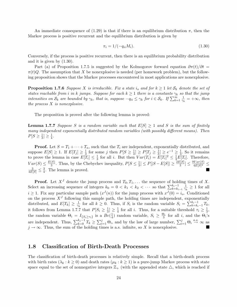
Proposition 1.7.6 Suppose X is irreducible. Fix a state io and for k ≥ 1 let Sk denote the set ofstates reachable from i in k jumps. Suppose for each k ≥ 1 there is a constants γk so that the jumpintensities on Sk are bounded by γk, that is, suppose −qii ≤ γk for i ∈ Sk. If

∑∞k=1

1γk

= +∞, thenthe process X is nonexplosive.

The proposition is proved after the following lemma is proved:

Lemma 1.7.7 Suppose S is a random variable such that E[S] ≥ 1 and S is the sum of finitelymany independent exponentially distributed random variables (with possibly different means). ThenP [S ≥ 1

3 ] ≥ 14 .

Proof. Let S = T1 + · · ·+Tn, such that the Ti are independent, exponentially distributed, andsuppose E[S] ≥ 1. If E[Tj ] ≥ 1

3 for some j then P [S ≥ 13 ] ≥ P [Tj ≥ 1

3 ] ≥ e−1 ≥ 13 . So it remains

to prove the lemma in case E[Ti] ≤ 13 for all i. But then V ar(Ti) = E[Ti]2 ≤ 1

3E[Ti]. Therefore,V ar(S) ≤ E(S)

3 . Thus, by the Chebychev inequality, P [S ≤ 13 ] ≤ P [|S−E[S]| ≥ 2E[S]

3 ] ≤ 9V ar(S)4E[S]2

≤3

4E[S] ≤34 . The lemma is proved.

Proof. Let XJ denote the jump process and T0, T1, . . . the sequence of holding times of X.Select an increasing sequence of integers k0 = 0 < k1 < k2 < · · · so that

∑ki−1k=ki−1

1γk≥ 1 for all

i ≥ 1. Fix any particular sample path (xJ(n)) for the jump process with xJ(0) = io. Conditionedon the process XJ following this sample path, the holding times are independent, exponentiallydistributed, and E[Tk] ≥ 1

γkfor all k ≥ 0. Thus, if Si is the random variable Si =

∑ki−1k=ki−1 Tk,

it follows from Lemma 1.7.7 that P [Si ≥ 13 ] ≥ 1

4 for all i. Thus, for a suitable threshold τi ≥ 13 ,

the random variable Θi = ISi≥τi is a Be(14) random variable, Si ≥ Θi

3 for all i, and the Θi’s

are independent. Thus,∑kj−1

k=0 Tk ≥∑j

i=1 Θi, and by the law of large number,∑j

i=1 Θia.s.→ ∞ as

j →∞. Thus, the sum of the holding times is a.s. infinite, so X is nonexplosive.

1.8 Classification of Birth-Death Processes

The classification of birth-death processes is relatively simple. Recall that a birth-death processwith birth rates (λk : k ≥ 0) and death rates (µk : k ≥ 1) is a pure-jump Markov process with statespace equal to the set of nonnegative integers Z+ (with the appended state 4, which is reached if

24

and only if infinitely many jumps occur in finite time), and generator matrix Q = (qij : i, j ≥ 0)given by

qij =

λi if j = i + 1µi if j = i− 1

−λi − µi if j = i ≥ 1−λi if j = i = 10 else.

(1.31)

Suppose that the birth and death rates are all strictly positive. Then the process is irreducible. Letbin denote the probability that, given the process starts in state i, it reaches state n without firstreaching state 0. Clearly b0n = 0 and bnn = 1. Fix i with 1 ≤ i ≤ n− 1, and derive an expressionfor bin by first conditioning on the state reached upon the first jump of the process, starting fromstate i. By the analysis of jump probabilities, the probability the first jump is up is λi/(λi + µi)and the probability the first jump is down is µi/(λi + µi). Thus,

bin =λi

λi + µibi+1,n +

µi

λi + µibi−1,n,

which can be rewritten as µi(bin − bi−1,n) = λi(bi+1,n − bi,n). In particular, b2n − b1n = b1nµ1/λ1

and b3n − b2n = b1nµ1µ2/(λ1λ2), and so on, which upon summing yields the expression

bkn = b1n

k−1∑i=0

µ1µ2 . . . µi

λ1λ2 . . . λi.

with the convention that the i = 0 term in the sum is zero. Finally, the condition bnn = 1 yieldsthe solution

b1n =1∑n−1

i=0µ1µ2...µi

λ1λ2...λi

. (1.32)

Note that b1n is the probability, for initial state 1, of the event Bn that state n is reached withoutan earlier visit to state 0. Since Bn+1 ⊂ Bn for all n ≥ 1,

P [∩n≥1Bn|X(0) = 1] = limn→∞

b1n = 1/S2 (1.33)

where S2 =∑∞

i=0 µ1µ2 . . . µi/λ1λ2 . . . λi, with the understanding that the i = 0 term in the sumdefining S2 is one. Due to the definition of pure jump processes used, whenever X visits a statein S the number of jumps up until that time is finite. Thus, on the event ∩n≥1Bn, state zero isnever reached. Conversely, if state zero is never reached, then either the process remains bounded(which has probability zero) or ∩n≥1Bn is true. Thus, P [zero is never reached|X(0) = 1] = 1/S2.Consequently, X is recurrent if and only if S2 = ∞.

Next, investigate the case S2 = ∞. Then the process is recurrent, so that in particular explosionhas probability zero, so that the process is positive recurrent if and only if πQ = 0.

Now πQ = 0 if and only if flow balance holds for any state k:

(λk + µk)πk = λk−1πk−1 + µk+1πk+1. (1.34)

Equivalently, flow balance must hold for all sets of the form 0, . . . , n−1, yielding that πn−1λn−1 =πnλn, or πn = π0λ0 . . . λn−1/(µ1 . . . µn). Thus, a probability distribution π with πQ = 0 exists ifand only if S1 < +∞, where

S1 =∞∑

n=0

λ0 . . . λn−1

µ1 . . . µn, (1.35)

25

with the understanding that the i = 0 term in the sum defining S1 is one. Still assuming S2 = ∞,such a probability distribution exists if and only if the Markov process is positive recurrent.

In summary, the following proposition is proved.

Proposition 1.8.1 If S2 < +∞ then all the states in Z+ are transient, and the process maybe explosive. If S2 = +∞ and S1 = +∞ then all states are null-recurrent. If S2 = +∞ andS1 < +∞ then all states are positive-recurrent and the equilibrium probability distribution is givenby πn = (λ0 . . . λn−1)/(S1µ1 . . . µn).

Discrete-time birth-death processes have a similar characterization. They are discrete-time,time-homogeneous Markov processes with state space equal to the set of nonnegative integers. Letnonnegative birth probabilities (λk : k ≥ 0) and death probabilities (µk : k ≥ 1) satisfy λ0 ≤ 1, andλk + µk ≤ 1 for k ≥ 1. The one-step transition probability matrix P = (pij : i, j ≥ 0) is given by

pij =

λi if j = i + 1µi if j = i− 1

1− λi − µi if j = i ≥ 11− λi if j = i = 1

0 else.

(1.36)

Implicit in the specification of P is that births and deaths can’t happen simultaneously. If the birthand death probabilities are strictly positive, Proposition 1.8.1 holds as before, with the exceptionthat the discrete-time process cannot be explosive. 3

1.9 Time Averages vs. Statistical Averages

Let X be a positive recurrent, irreducible, time-homogeneous Markov process with equilibriumprobability distribution π. To be definite, suppose X is a continuous-time process, with pure-jumpsample paths and generator matrix Q. The results of this section apply with minor modifica-tions to the discrete-time setting as well. Above it is shown that renewal theory implies thatlimt→∞ πi(t) = πi = 1/(−qiiMi), where Mi is the mean “cycle time” of state i. A related con-sideration is convergence of the empirical distribution of the Markov process, where the empiricaldistribution is the distribution observed over a (usually large) time interval.

For a fixed state i, the fraction of time the process spends in state i during [0, t] is

1t

∫ t

0IX(s)=ids

Let T0 denote the time that the process is first in state i, and let Tk for k ≥ 1 denote the timethat the process jumps to state i for the kth time after T0. The cycle times Tk+1 − Tk, k ≥ 0 areindependent and identically distributed, with mean Mi. Therefore, by the law of large numbers,with probability one,

limk→∞

Tk/k = limk→∞

1k

k−1∑l=0

(Tl+1 − Tl) (1.37)

= Mi (1.38)3If in addition λi + µi = 1 for all i, then the discrete time process has period 2.

26

Furthermore, during the kth cycle interval [Tk, Tk+1), the amount of time spent by the processin state i is exponentially distributed with mean −1/qii, and the time spent in the state duringdisjoint cycles is independent. Thus, with probability one,

limk→∞

1k

∫ Tk

0IX(s)=idt = lim

k→∞

1k

k−1∑l=0

∫ Tl+1

Tl

IX(s)=ids (1.39)

= E[∫ T1

T0

IX(s)=ids] (1.40)

= −1/qii (1.41)

Combining these two observations yields that

limt→∞

1t

∫ t

0IX(s)=ids = 1/(−qiiMi) = πi (1.42)

with probability one. In short, the limit (1.42) is expected, because the process spends on average−1/qii time units in state i per cycle from state i, and the cycle rate is 1/Mi. Of course, since statei is arbitrary, if j is any other state then

limt→∞

1t

∫ t

0IX(s)=jds = 1/(−qjjMj) = πj (1.43)

By considering how the time in state j is distributed among the cycles from state i, it follows thatthe mean time spent in state j per cycle from state i is Miπj .

So for any nonnegative function φ on S,

limt→∞

1t

∫ t

0φ(X(s))ds = lim

k→∞

1kMi

∫ Tk

0φ(X(s))ds

=1

MiE

[∫ T1

T0

φ(X(s))ds

]

=1

MiE

∑j∈S

φ(j)∫ T1

T0

IX(s)=jds

=

1Mi

∑j∈S

φ(j)E[∫ T1

T0

IX(s)=j

]ds

=∑j∈S

φ(j)πj (1.44)

Finally, if φ is a function of S such that either∑

j∈S φ+(j)πj < ∞ or∑

j∈S φ−(j)πj < ∞, thensince (1.44) holds for both φ+ and φ−, it must hold for φ itself.

1.10 Queueing Systems, M/M/1 Queue and Little’s Law

Some basic terminology of queueing theory will now be explained. A simple type of queueing systemis pictured in Figure 1.13. Notice that the system is comprised of a queue and a server. Ordinarily

27

queue server

system

Figure 1.13: A single server queueing system

whenever the system is not empty, there is a customer in the server, and any other customers inthe system are waiting in the queue. When the service of a customer is complete it departs fromthe server and then another customer from the queue, if any, immediately enters the server. Thechoice of which customer to be served next depends on the service discipline. Common servicedisciplines are first-come first-served (FCFS) in which customers are served in the order of theirarrival, or last-come first-served (LCFS) in which the customer that arrived most recently is servednext. Some of the more complicated service disciplines involve priority classes, or the notion of“processor sharing” in which all customers present in the system receive equal attention from theserver.

Often models of queueing systems involve a stochastic description. For example, given positiveparameters λ and µ, we may declare that the arrival process is a Poisson process with rate λ,and that the service times of the customers are independent and exponentially distributed withparameter µ. Many queueing systems are given labels of the form A/B/s, where “A” is chosen todenote the type of arrival process, “B” is used to denote the type of departure process, and s isthe number of servers in the system. In particular, the system just described is called an M/M/1queueing system, so-named because the arrival process is memoryless (i.e. a Poisson arrival process),the service times are memoryless (i.e. are exponentially distributed), and there is a single server.Other labels for queueing systems have a fourth descriptor and thus have the form A/B/s/b, whereb denotes the maximum number of customers that can be in the system. Thus, an M/M/1 systemis also an M/M/1/∞ system, because there is no finite bound on the number of customers in thesystem.

A second way to specify an M/M/1 queueing system with parameters λ and µ is to let A(t) andD(t) be independent Poisson processes with rates λ and µ respectively. Process A marks customerarrival times and process D marks potential customer departure times. The number of customers inthe system, starting from some initial value N(0), evolves as follows. Each time there is a jump ofA, a customer arrives to the system. Each time there is a jump of D, there is a potential departure,meaning that if there is a customer in the server at the time of the jump then the customer departs.If a potential departure occurs when the system is empty then the potential departure has no effecton the system. The number of customers in the system N can thus be expressed as

N(t) = N(0) + A(t) +∫ t

0IN(s−)≥1dD(s)

It is easy to verify that the resulting process N is Markov, which leads to the third specification ofan M/M/1 queueing system.

28

t

!

" ss

s

N(s)

Figure 1.14: A single server queueing system

A third way to specify an M/M/1 queuing system is that the number of customers in the systemN(t) is a birth-death process with λk = λ and µk = µ for all k, for some parameters λ and µ. Letρ = λ/µ. Using the classification criteria derived for birth-death processes, it is easy to see thatthe system is recurrent if and only if ρ ≤ 1, and that it is positive recurrent if and only if ρ < 1.Moreover, if ρ < 1 then the equilibrium distribution for the number of customers in the system isgiven by πk = (1− ρ)ρk for k ≥ 0. This is the geometric distribution with zero as a possible value,and with mean

N =∞∑

k=0

kπk = (1− ρ)ρ∞∑

k=1

ρk−1k = (1− ρ)ρ(1

1− ρ)′ =

ρ

1− ρ

The probability the server is busy, which is also the mean number of customers in the server, is1−π0 = ρ. The mean number of customers in the queue is thus given by ρ/(1−ρ)−ρ = ρ2/(1−ρ).This third specification is the most commonly used way to define an M/M/1 queueing process.

Since the M/M/1 process N(t) is positive recurrent, the Markov ergodic convergence theoremimplies that the statistical averages just computed, such as N , are also equal to the limit of thetime-averaged number of customers in the system as the averaging interval tends to infinity.

An important performance measure for a queueing system is the mean time spent in the systemor the mean time spent in the queue. Littles’ law, described next, is a quite general and usefulrelationship that aids in computing mean transit time.

Little’s law can be applied in a great variety of circumstances involving flow through a systemwith delay. In the context of queueing systems we speak of a flow of customers, but the sameprinciple applies to a flow of water through a pipe. Little’s law is that λT = N where λ is themean flow rate, T is the mean delay in the system, and N is the mean content of the queue. Forexample, if water flows through a pipe with volume one cubic meter at the rate of two cubic metersper minute, then the mean time (averaged over all drops of water) that water spends in the pipe isT = N/λ = 1/2 minute. This is clear if water flows through the pipe without mixing, for then thetransit time of each drop of water is 1/2 minute. However, mixing within the pipe does not effectthe average transit time.

Little’s law is actually a set of results, each with somewhat different mathematical assumptions.

29

The following version is quite general. Figure 1.14 pictures the cumulative number of arrivals (α(t))and the cumulative number of departures (δ(t)) versus time, for a queueing system assumed to beinitially empty. Note that the number of customers in the system at any time s is given by thedifference N(s) = α(s) − δ(s), which is the vertical distance between the arrival and departuregraphs in the figure. On the other hand, assuming that customers are served in first-come first-served order, the horizontal distance between the graphs gives the times in system for the customers.Given a (usually large) t > 0, let γt denote the area of the region between the two graphs over theinterval [0, t]. This is the shaded region indicated in the figure. It is then natural to define thetime-averaged values of arrival rate and system content as

λt = α(t)/t and N t =1t

∫ t

0N(s)ds = γt/t

Finally, the average, over the α(t) customers that arrive during the interval [0, t], of the time spentin the system up to time t, is given by

T t = γt/α(t).

Once these definitions are accepted, we have the obvious simple relation:

N t = λtT t (1.45)

Consider next (1.45) in the limit as t →∞. If any two of the three variables in (1.45) converge tofinite positive quantities, then so does the third variable, and in the limit Little’s law is obtained.

For example, the number of customers in an M/M/1 queue is a positive recurrent Markovprocess so that

limt→∞

N t = N = ρ/(1− ρ)

where calculation of the statistical mean N was previously discussed. Also, by the weak renewaltheorem or the law of large numbers applied to interarrival times, we have that the Poisson arrivalprocess for an M/M/1 queue satisfies limt→∞ λt = λ with probability one. Thus,

limt→∞

T t = N/λ =1

µ− λ.

In this sense, the average waiting time in an M/M/1 system is 1/(µ−λ). The average time in serviceis 1/µ (this follows from the third description of an M/M/1 queue, or also from Little’s law appliedto the server alone) so that the average waiting time in queue is given by W = 1/(µ− λ)− 1/µ =ρ/(µ− λ). This final result also follows from Little’s law applied to the queue alone.

1.11 Mean Arrival Rate, Distributions Seen by Arrivals, and PASTA

The mean arrival rate for the M/M/1 system is λ, the parameter of the Poisson arrival process.However for some queueing systems the arrival rate depends on the number of customers in thesystem. In such cases the mean arrival rate is still typically meaningful, and it can be used inLittle’s law.

Suppose the number of customers in a queuing system is modeled by a birth death processwith arrival rates (λk) and departure rates (µk). Suppose in addition that the process is positive

30

recurrent. Intuitively, the process spends a fraction of time πk in state k and while in state k thearrival rate is λk. Therefore, the average arrival rate is

λ =∞∑

k=0

πkλk

Similarly the average departure rate is

µ =∞∑

k=1

πkµk

and of course λ = µ because both are equal to the throughput of the system.Often the distribution of a system at particular system-related sampling times are more impor-

tant than the distribution in equilibrium. For example, the distribution seen by arriving customersmay be the most relevant distribution, as far as the customers are concerned. If the arrival ratedepends on the number of customers in the system then the distribution seen by arrivals need notbe the same as the equilibrium distribution. Intuitively, πkλk is the long-term frequency of arrivalswhich occur when there are k customers in the system, so that the fraction of customers that seek customers in the system upon arrival is given by

rk =πkλk

λ.

The following is an example of a system with variable arrival rate.Example 1.5 (Single-server, discouraged arrivals)Suppose λk = α/(k + 1) and µk = µ for all k, where µ and α are positive constants. Then

S2 =∞∑

k=0

(k + 1)!µk

αk= ∞ and S1 =

∞∑k=0

αk

k!µk= exp(

α

µ) < ∞

so that the number of customers in the system is a positive recurrent Markov process, with noadditional restrictions on α and µ. Moreover, the equilibrium probability distribution is given byπk = (α/µ)k exp(−α/µ)/k!, which is the Poisson distribution with mean N = α/µ. The meanarrival rate is

λ =∞∑

k=0

πkα

k + 1= µ exp(−α

µ)∞∑

k=0

(α/µ)k+1

(k + 1)!= µ exp(−α

µ)(exp(

α

µ)− 1) = µ(1− exp(−α

µ)). (1.46)

This expression derived for λ is clearly equal to µ, because the departure rate is µ with probability1 − π0 and zero otherwise. The distribution of the number of customers in the system seen byarrivals, (rk) is given by

rk =πkα

(k + 1)λ=

(α/µ)k+1 exp(−α/µ)(k + 1)!(1− exp(−α/µ))

for k ≥ 0

which in words can be described as the result of removing the probability mass at zero in thePoisson distribution, shifting the distribution down by one, and then renormalizing. The meannumber of customers in the queue seen by a typical arrival is therefore (α/µ− 1)/(1− exp(−α/µ)).

31

This mean is somewhat less than N because, roughly speaking, the customer arrival rate is higherwhen the system is more lightly loaded.

The equivalence of time-averages and statistical averages for computing the mean arrival rateand the distribution seen by arrivals can be shown by application of ergodic properties of theprocesses involved. The associated formal approach is described next, in slightly more generality.Let X denote an irreducible, positive-recurrent pure-jump Markov process. If the process makes ajump from state i to state j at time t, say that a transition of type (i, j) occurs. The sequence oftransitions of X forms a new Markov process, Y . The process Y is a discrete-time Markov processwith state space (i, j) ∈ S ×S : qij > 0, and it can be described in terms of the jump process forX, by Y (k) = (XJ(k − 1), XJ(k)) for k ≥ 0. (Let XJ(−1) be defined arbitrarily.)

The one-step transition probability matrix of the jump process XJ is given by πJij = qij/(−qii),

and XJ is recurrent because X is recurrent. Its equilibrium distribution πJ (if it exists) is propor-tional to −πiqii (see problem set 1), and XJ is positive recurrent if and only if this distribution canbe normalized to make a probability distribution, i.e. if and only if R = −

∑i πiqii < ∞. Assume

for simplicity that XJ is positive recurrent. Then πJi = −πiqii/R is the equilibrium probability

distribution of XJ . Furthermore, Y is positive recurrent and its equilibrium distribution is givenby

πYij = πJ

i pJij

=−πiqii

R

qij

−qii

=πiqij

R

Since limiting time averages equal statistical averages for Y ,

limn→∞

(number of first n transitions of X that are type (i, j))/n = πiqij/R

with probability one. Therefore, if A ⊂ S × S, and if i ∈ A, then

limn→∞

number of first n transitions of X that are type (i, j)number of first n transitions of X with type in A

=πiqij∑

(i′,j′)∈A πi′qi′j′(1.47)

We remark (1.47) is still true if the assumption R < ∞ is replaced by the weaker assumption thatthe denominator on the righthand side of (1.47) is finite. In case R = ∞ the statement is then aninstance of a ratio limit theorem for recurrent (not necessarily positive recurrent) Markov processes.

To apply this setup to the special case of a queueing system in which the number of customersin the system is a Markov birth-death processes, let the set A be the set of transitions of the form(i, i + 1). Then deduce that the fraction of the first n arrivals that see i customers in the systemupon arrival converges to πiλi/

∑j πjλj with probability one.

Note that if λi = λ for all i, then λ = λ and π = r. The condition λi = λ also implies that thearrival process is Poisson. This situation is called “Poisson Arrivals See Time Averages” (PASTA).

1.12 More Examples of Queueing Systems Modeled as MarkovBirth-Death Processes

For each of the four examples of this section it is assumed that new customers are offered to thesystem according to a Poisson process with rate λ, so that the PASTA property holds. Also, when

32

there are k customers in the system then the service rate is µk for some given numbers µk. Thenumber of customers in the system is a Markov birth-death process with λk = λ for all k. Sincethe number of transitions of the process up to any given time t is at most twice the number ofcustomers that arrived by time t, the Markov process is not explosive. Therefore the process ispositive recurrent if and only if S1 is finite, where

S1 =∞∑

k=0

λk

µ1µ2 . . . µk

Special cases of this example are presented in the next four examples.Example 1.6 (M/M/m systems) An M/M/m queueing system consists of a single queue and

m servers. The arrival process is Poisson with some rate λ and the customer service times areindependent and exponentially distributed with mean µ for some µ > 0. The total number ofcustomers in the system is a birth-death process with µk = µmin(k, m). Let ρ = λ/(mµ). Sinceµk = mµ for all k large enough it is easy to check that the process is positive recurrent if and onlyif ρ < 1. Assume now that ρ < 1. Then the equilibrium distribution is given by

πk =(λ/µ)k

S1k!for 0 ≤ k ≤ m

πm+j = πmρj for j ≥ 1

where S1 is chosen to make the probabilities sum to one (use the fact 1 + ρ + ρ2 . . . = 1/(1− ρ)):

S1 =

(m−1∑k=0

(λ/µ)k

k!

)+

(λ/µ)m

m!(1− ρ).

An arriving customer must join the queue (rather that go directly to a server) if and only if thesystem has m or more customers in it. By the PASTA property, this is the same as the equilibriumprobability of having m or more customers in the system:

PQ =∞∑

j=0

πm+j = πm/(1− ρ)

This formula is called the Erlang C formula for probability of queueing.Example 1.7 (M/M/m/m systems) An M/M/m/m queueing system consists of m servers.

The arrival process is Poisson with some rate λ and the customer service times are independentand exponentially distributed with mean µ for some µ > 0. Since there is no queue, if a customerarrives when there are already m customers in the system, then the arrival is blocked and clearedfrom the system. The total number of customers in the system is a birth death process, but withthe state space reduced to 0, 1, . . . ,m, and with µk = kµ for 1 ≤ k ≤ m. The unique equilibriumdistribution is given by

πk =(λ/µ)k

S1k!for 0 ≤ k ≤ m

where S1 is chosen to make the probabilities sum to one.An arriving customer is blocked and cleared from the system if and only if the system already

has m customers in it. By the PASTA property, this is the same as the equilibrium probability of

33

having m customers in the system:

PB = πm =(λ/µ)m

m!∑mj=0

(λ/µ)j

j!

This formula is called the Erlang B formula for probability of blocking.Example 1.8 (A system with a discouraged server) The number of customers in this system

is a birth-death process with constant birth rate λ and death rates µk = 1/k. It is is easy tocheck that all states are transient for any positive value of λ (to verify this it suffices to check thatS2 < ∞). It is not difficult to show that N(t) converges to +∞ with probability one as t →∞.

Example 1.9 (A barely stable system) The number of customers in this system is a birth-deathprocess with constant birth rate λ and death rates µk = λ(1+k2)

1+(k−1)2for all k ≥ 1. Since the departure

rates are barely larger than the arrival rates, this system is near the borderline between recurrenceand transience. However, we see that

S1 =∞∑

k=0

11 + k2

< ∞

so that N(t) is positive recurrent with equilibrium distribution πk = 1/(S1(1 + k2)). Note that themean number of customers in the system is

N =∞∑

k=0

k/(S1(1 + k2)) = ∞

By Little’s law the mean time customers spend in the system is also infinity. It is debatable whetherthis system should be thought of as “stable” even though all states are positive recurrent and allwaiting times are finite with probability one.

1.13 Method of Phases and Quasi Birth-Death Processes

The method of phases in a broad sense refers to approximating general probability distributions bysums and mixtures of exponential distributions. Such distributions can be obtained as the hittingtime of a target state of a finite state Markov process. The state of the Markov process at a giventime represents the “phase” of the distribution. The method permits Markov processes to modelsystems in which the original distributions are not exponential.

To illustrate the method here we consider the class of random processes called quasi birth anddeath (QBD) processes. These processes generalize M/M/1 queueing models in that the arrival anddeparture rates depend on the state of a phase process. (For more background, see M.F. Neuts,Matrix-Geometric Solutions in Stochastic Models – An Algorithmic Approach, The Johns HopkinsUniversity Press, Baltimore, MD, 1981 and B. Hajek, Birth-and-Death Processes on the Integerswith Phases and General Boundaries, Journal of Applied Probability, pp. 488-499, 1982.

Let k be a positive integer, denoting the number of possible phases. A QBD process is a time-homogeneous Markov process. The state space of the process is the set S equal to (l, θ) : l ≥1, 1 ≤ θ ≤ k. We call l the level and θ the phase of the state (l, θ). Here we shall restrict our

34

attention to continuous time processes. Let A0, A1, A2, and A00 denote k × k matrices so that thematrix Q∗ defined by

Q∗ =

A00 A2

A0 A1 A2

A0 A1 A2

A0 A1 A2

. . .. . .

(1.48)

is a generator matrix for the state space S. Equivalently, the matrices A0 and A2 have nonnegativeentries, the matrices A1 and A00 have nonnegative off-diagonal entries and nonpositive diagonalentries, the matrix Q defined by Q = A0 + A1 + A2 and the matrix A00 + A2 both have row sumsequal to zero.

Suppose that Q∗ and Q are both irreducible. Define π to be the equilibrium probability vectorfor Q, so that πQ = 0 and set µ = πA2e− πA0e where e is the k vector of all ones. Then all statesare positive recurrent for Q∗ if and only if µ < 0. If µ < 0 then the equilibrium distribution for Q∗

is given by (x0, x1, . . .) where

x0 = π0/c, xk = x0Rk, c = π0(I −R)−1e,R = A2B (1.49)

where π0 is the equilibrium probability distribution for a k-state Markov process with generatormatrix A00 + A01BA10, and B is the minimal positive solution to

B = −(A1 + A2BA0)−1 (1.50)

An effective numerical procedure for finding B is to iterate equation (1.50). In other words, setB(0) to be the matrix of all zeros, and sequentially compute B(n) by B(n) = −(A1+A2B

(n−1)A0)−1.

Exercises1. Let (Lt,Θt) denote the QBD process. Under what conditions on A0, A1, A2 and A00 is theprocess (Θt) a Markov process? Prove your answer.2. Consider the following variation of an M/M/1 queue. There is a two state Markov process withstates 1 and 2 and transition rates q12 = 1 and q21 = 2. The two state process is a phase process forthe queue. When the phase is 1 there are no arrivals to the queue, and when the phase is 2 arrivalsoccur at an average rate of 2 customers per second, according to a Poisson process. Service times ofall customers are independent and exponentially distributed with mean one. Suppose a QBD modelis used. What values of the matrices A0, A1, A2 and A00 should be used? Find (numerical solutionOK) B,R, and the equilibrium distribution (xl)l≥0. Finally, describe the equilibrium probabilitydistribution of the number of customers in the system. (Solution:

A0 =(

1 00 1

)A1 =

(−2 12 −5

)A2 =

(0 00 2

)(1.51)

A00 =(−1 12 −4

)B =

(0.8090 0.19100.6179 0.3819

)R =

(0 0

1.236 0.764

)(1.52)

xk = (.764)k(0.1273, 0.0787) for k ≥ 1 and x0 = (0.255, 0.0787). In equilibrium, P [L = l] =(0.206)(0.764)l for l ≥ 1 and P [L = 0] = 1/3. Thus, the distribution for L is a mixture of thegeometric distribution and a distribution concentrated at zero.

35

1.14 Markov Fluid Model of a Queue

A limiting form of quasi birth and death processes is a queue with a Markov-modulated rate ofarrival, which is briefly described in this section. See D. Mitra, “Stochastic Theory of a FluidModel of Producers and Consumers Coupled by a Buffer”, Annals of Applied Probability, Vol. 20,pp. 646-676, 1988 for more information.

Let Q be the generator matrix of an irreducible Markov process with state space 1, . . . ,m.Suppose there is a buffer and that when the process is in state i, the net rate (arrival rate minusdeparture rate) of flow of fluid into the buffer is di. The only exception to this rule is that if thebuffer is empty and the Markov process is in a state i such that di ≤ 0 then the buffer simplyremains empty. Let D denote the diagonal matrix with d1, . . . , dm along the diagonal. See Figure1.15.

"!#

- -

JJ

JJ

JJ]

Markov process determines

(input rate) - (output rate)

Figure 1.15: Fluid queue with net input rate determined by a Markov process

The average drift is defined to be∑m

i=1 widi, or wDe, where w is the equilibrium probabilitydistribution for the finite state Markov process and e is the column vector of all 1’s.

Let Lt denote the level of fluid in the buffer at time t and let θt denote the state of the finiteMarkov process at time t. Then (Lt, θt) is a continuous state Markov process, and is a limitingform of a quasi birth-death process. In the remainder of this section we describe how to find theequilibrium distribution of this process.

Let F (x, i, t) = P [θt = i, Lt ≤ x]. Kolmogorov’s forward equations are derived by beginningwith the observation

F (x, i, t + h) = hm∑

j=1

F (x, j, t)qi,j + o(h) + F (x− hdi, i, t). (1.53)

Subtracting F (x, i, t) from each side of this equation and letting h → 0 yields

∂F (x, i, t)∂t

=m∑

j=1

F (x, j, t)qj,i −∂F (x, i, t)

∂xdi (1.54)

or in matrix notation, letting F (t) denote the row vector F (t) = (F (x, 1, t), . . . , F (x,m, t)),

∂F

∂t= FQ− ∂F

∂xD (1.55)

36

Conditions on the equilibrium distribution F (x, i) are found by setting ∂F∂t = 0, yielding the equation

FQ = ∂F∂x D. By definition, we know F (∞, i) = wi. Motivated by this and the theory of linear

systems, we seek a solution of the form

F (x, i) = w −k∑

i=1

aiφiexzi (1.56)

where (φi, zi) are eigenvalue-eigenvector pairs, meaning that φiQ = ziφiD.To avoid substantial technical complications, we make the assumption that Q is reversible,

meaning that wiqi,j = wjqj,i for 1 ≤ i, j ≤ m. Then all the eigenvalues are real valued. Letk = |i : di > 0|. It can be shown that there are k strictly negative eigenvalues (countingmultiplicity) and those are the ones to be included in the sum in (1.56). Finally, the k coefficientsa1, . . . , ak can be found by satisfying the k boundary conditions:

F (0, i) = 0 whenever di > 0 (1.57)

For example, suppose

Q =(−1 12 −2

)and D =

(−1 00 1

)(1.58)

We compute that w = (23 , 1

3) and that (F (x, 1), F (x, 2)) = (2−exp(−x)3 , 1−exp(−x)

3 ). In particular, inequilibrium, P [Lt ≥ x] = 2 exp(−x)

3 .

1.15 Problems

1.1. Poisson mergerSumming counting processes corresponds to “merging” point processes. Show that the sum of Kindependent Poisson processes, having rates λ1, . . . , λK , respectively, is a Poisson process with rateλ1 + . . . + λK . (Hint: First formulate and prove a similar result for sums of random variables, andthen think about what else is needed to get the result for Poisson processes. You can use any oneof the equivalent definitions given by Proposition 1.5.1 in the notes. Don’t forget to check requiredindependence properties.)

1.2. Poisson splittingConsider a stream of customers modeled by a Poisson process, and suppose each customer is oneof K types. Let (p1, . . . , pK) be a probability vector, and suppose that for each k, the kth customeris type i with probability pi. The types of the customers are mutually independent and also inde-pendent of the arrival times of the customers. Show that the stream of customers of a given type iis again a Poisson stream, and that its rate is λpi. (Same hint as in the previous problem applies.)Show furthermore that the K substreams are mutually independent.

1.3. Poisson method for coupon collector’s problem(a) Suppose a stream of coupons arrives according to a Poisson process (A(t) : t ≥ 0) with rateλ = 1, and suppose there are k types of coupons. (In network applications, the coupons could bepieces of a file to be distributed by some sort ot gossip algorithm.) The type of each coupon in the

37

stream is randomly drawn from the k types, each possibility having probability 1k , and the types of

different coupons are mutually independent. Let p(k, t) be the probability that at least one couponof each type arrives by time t. (The letter “p” is used here because the number of coupons arrivingby time t has the Poisson distribution). Express p(k, t) in terms of k and t.(b) Find limk→∞ p(k, k ln k + kc) for an arbitrary constant c. That is, find limit of the proba-bility that the collection is complete at time t = k ln k + kc. (Hint: If ak → a as k → ∞, then(1 + ak

k )k → ea.)(c) The rest of this problem shows that the limit found in part (b) also holds if the total number ofcoupons is deterministic, rather than Poisson distributed. One idea is that if t is large, then A(t)is not too far from its mean with high probability. Show, specifically, that

limk→∞ P [A(k ln k + kc) ≥ k ln k + kc′] =

0 if c < c′

1 if c > c′

(d) Let d(k, n) denote the probability that the collection is complete after n coupon arrivals. (Theletter “d” is used here because the number of coupons, n, is deterministic.) Show that for any k, t,and n fixed, d(k, n)P [A(t) ≥ n] ≤ p(k, t) ≤ P [A(t) ≥ n] + P [A(t) ≤ n]d(k, n).(e) Combine parts (c) and (d) to identify limk→∞ d(k, k ln k + kc).

1.4. The sum of a random number of random variablesLet (Xi : i ≥ 0) be a sequence of independent and identically distributed random variables. LetS = X1 + . . .+XN , where N is a nonnegative random variable that is independent of the sequence.(a) Express E[S] and V ar(S) in terms of the mean and variance of X1 and N . (Hint: Use thefact E[Sk] = E[E[Sk|N ]]). (b) Express the characteristic function ΦS in terms of the characteristicfunction ΦX of X1 and the z-transform B(z) of N .

1.5. Mean hitting time for a simple Markov processLet (X(n) : n ≥ 0) denote a discrete-time, time-homogeneous Markov chain with state space0, 1, 2, 3 and one-step transition probability matrix

P =

0 1 0 0

1− a 0 a 00 0.5 0 0.50 0 1 0

for some constant a with 0 ≤ a ≤ 1. (a) Sketch the transition probability diagram for X andgive the equilibrium probability vector. If the equilibrium vector is not unique, describe all theequilibrium probability vectors.(b) Compute E[minn ≥ 1 : X(n) = 3|X(0) = 0].

1.6. A two station pipeline in continuous timeConsider a pipeline consisting of two single-buffer stages in series. Model the system as a continuous-time Markov process. Suppose new packets are offered to the first stage according to a rate λ Poissonprocess. A new packet is accepted at stage one if the buffer in stage one is empty at the time ofarrival. Otherwise the new packet is lost. If at a fixed time t there is a packet in stage one andno packet in stage two, then the packet is transfered during [t, t + h) to stage two with probabilityhµ1 + o(h). Similarly, if at time t the second stage has a packet, then the packet leaves the systemduring [t, t + h) with probability hµ2 + o(h), independently of the state of stage one. Finally, theprobability of two or more arrival, transfer, or departure events during [t, t + h) is o(h). (a) What

38

is an appropriate state-space for this model? (b) Sketch a transition rate diagram. (c) Write downthe Q matrix. (d) Derive the throughput, assuming that λ = µ1 = µ2 = 1. (e) Still assumingλ = µ1 = µ2 = 1. Suppose the system starts with one packet in each stage. What is the expectedtime until both buffers are empty?

1.7. Simple population growth modelsA certain population of living cells begins with a single cell. Each cell present at a time t splitsinto two cells during the interval [t, t + h] with probability λh + o(h), independently of the othercells, for some constant λ > 0. The number of cells at time t, N(t), can thus be modeled as acontinuous-time Markov chain. (a) Sketch an appropriate transition rate diagram and describe thetransition rate matrix. (b) For fixed t ≥ 0, let P (z, t) denote the z-transform of the probabilityvector π(t). Starting with the Kolmogorov forward equations for (π(t)), derive a partial differentialequation for the z-transform of π(t). Show that the solution is

P (z, t) =ze−λt

1− z + ze−λt

(c) Find E[N(t)]. (d) Solve for π(t). (e) Another population evolves deterministically. The first cellsplits at time λ−1, and thereafter each cell splits into two exactly λ−1 time units after its creation.Find the size of the population of this population as a function of time, and compare to your answerin part (c).

1.8. Equilibrium distribution of the jump chainSuppose that π is the equilibrium distribution for a time-homogeneous Markov process with tran-sition rate matrix Q. Suppose that B−1 =

∑i−qiiπi, where the sum is over all i in the state space,

is finite. Show that the equilibrium distribution for the jump chain (XJ(k) : k ≥ 0) is given byπJ

i = −Bqiiπi. (So π and πJ are identical if and only if qii is the same for all i.)

1.9. A simple Poisson process calculation1. Let (N(t) : t ≥ 0) be a Poisson random process with rate λ > 0. Compute P [N(s) = i|N(t) = k]where 0 < s < t and i and k are nonnegative integers. (Caution: note order of s and t carefully).

1.10. An alternating renewal processConsider a two-color traffic signal on a street corner which alternately stays red for one minute andthen stays green for one minute. Suppose you are riding your bicycle towards the signal and area block away when you first spot it, so that it will take you one-half minute to reach the signal.(a) What is the probability that the signal will change colors (at least once) before you reach thecorner? Explain. (b) Compute the conditional expectation of how long you must wait at the corner(possibly not at all) given that the light is green when you first spot it. Repeat assuming the lightis red when you first spot it. (Which is greater? What is the average of the two answers?) (c)Repeat part (a) if instead the signal randomly changes colors, staying the same color for a timeperiod uniformly distributed between 0 and 2 minutes. The times between switches are assumedto be independent. (d) How fast are you riding? (Hint: What units of speed can you use so thatyou don’t need more information?)

1.10.5. A simple question of periods3. (5 points ) Consider a discrete-time Markov process with the nonzero one-step transition prob-

39

abilities indicated by the following graph.

8

3

4

1 2

5 6

7

(a) What is the period of state 4?(b) What is the period of state 6?

1.11. A mean hitting time problemLet (X(t) : t ≥ 0) be a time-homogeneous, pure-jump Markov process with state space 0, 1, 2and Q matrix

Q =

−4 2 21 −2 12 0 −2.

(a) Write down the state transition diagram and compute the equilibrium distribution.(b) Compute ai = E[mint ≥ 0 : X(t) = 1|X(0) = i] for i = 0, 1, 2. If possible, use an approachthat can be applied to larger state spaces.(c) Derive a variation of the Kolmogorov forward differential equations for the quantities: αi(t) =P [X(s) 6= 2 for 0 ≤ s ≤ t and X(t) = i|X(0) = 0] for 0 ≤ i ≤ 2. (You need not solve theequations.)(d) The forward Kolmogorov equations describe the evolution of an initial probability distribu-tion going forward in time, given an initial. In other problems, a boundary condition is givenat a final time, and a differential equation working backwards in time from a final condition iscalled for (called Kolmogorov backward equations). Derive a backward differential equation for:βj(t) = P [X(s) 6= 2 for t ≤ s ≤ tf |X(t) = j], for 0 ≤ j ≤ 2 and t ≤ tf for some fixed time tf . (Hint:Express βi(t−h) in terms of the βj(t)′s for t ≤ tf , and let h → 0. You need not solve the equations.)

1.12. A birth-death process with periodic ratesConsider a single server queueing system in which the number in the system is modeled as acontinuous time birth-death process with the transition rate diagram shown, where λa, λb, µa, andµb are strictly positive constants.

a

31 20 . . .4

! ! !!

µ

!

µµ µ µ

a a ab b

a b a b

(a) Under what additional assumptions on these four parameters is the process positive recurrent?(b) Assuming the system is positive recurrent, under what conditions on λa, λb, µa, and µb is it truethat the distribution of the number in the system at the time of a typical arrival is the same as theequilibrium distribution of the number in the system?

40

1.13. Markov model for a link with resetsSuppose that a regulated communication link resets at a sequence of times forming a Poissonprocess with rate µ. Packets are offered to the link according to a Poisson process with rate λ.Suppose the link shuts down after three packets pass in the absence of resets. Once the link isshut down, additional offered packets are dropped, until the link is reset again, at which time theprocess begins anew.

!

µ

(a) Sketch a transition rate diagram for a finite state Markov process describing the system state.(b) Express the dropping probability (same as the long term fraction of packets dropped) in termsof λ and µ.

1.14. An unusual birth-death processConsider the birth-death process X with arrival rates λk = (p/(1 − p))k/ak and death ratesµk = (p/(1 − p))k−1/ak, where .5 < p < 1, and a = (a0, a1, . . .) is a probability distributionon the nonnegative integers with ak > 0 for all k. (a) Classify the states for the process X as tran-sient, null-recurrent or positive recurrent. (b) Check that aQ = 0. Is a an equilibrium distributionfor X? Explain. (c) Find the one-step transition probabilities for the jump-chain, XJ (d) Classifythe states for the process XJ as transient, null-recurrent or positive recurrent.

1.15. A queue with decreasing service rateConsider a queueing system in which the arrival process is a Poisson process with rate λ. Supposethe instantaneous completion rate is µ when there are K or fewer customers in the system, and µ/2when there are K + 1 or more customers in the system. The number in the system is modeled as abirth-death Markov process. (a) Sketch the transition rate diagram. (b) Under what condition onλ and µ are all states positive recurrent? Under this condition, give the equilibrium distribution.(c) Suppose that λ = (2/3)µ. Describe in words the typical behavior of the system, given that it isinitially empty.

1.16. Limit of a distrete time queueing systemModel a queue by a discrete-time Markov chain by recording the queue state after intervals of qseconds each. Assume the queue evolves during one of the atomic intervals as follows: There is anarrival during the interval with probability αq, and no arrival otherwise. If there is a customer inthe queue at the beginning of the interval then a single departure will occur during the intervalwith probability βq. Otherwise no departure occurs. Suppose that it is impossible to have anarrival and a departure in a single atomic interval. (a) Find ak=P[an interarrival time is kq] andbk=P[a service time is kq]. (b) Find the equilibrium distribution, p = (pk : k ≥ 0), of the numberof customers in the system at the end of an atomic interval. What happens as q → 0?

1.17. An M/M/1 queue with impatient customersConsider an M/M/1 queue with parameters λ and µ with the following modification. Each cus-tomer in the queue will defect (i.e. depart without service) with probability αh+o(h) in an intervalof length h, independently of the other customers in the queue. Once a customer makes it to

41

the server it no longer has a chance to defect and simply waits until its service is completed andthen departs from the system. Let N(t) denote the number of customers in the system (queue plusserver) at time t. (a) Give the transition rate diagram and generator matrix Q for the Markov chainN = (N(t) : t ≥ 0). (b) Under what conditions are all states positive recurrent? Under this condi-tion, find the equilibrium distribution for N . (You need not explicitly sum the series.) (c) Supposethat α = µ. Find an explicit expression for pD, the probability that a typical arriving customerdefects instead of being served. Does your answer make sense as λ/µ converges to zero or to infinity?

1.18. Statistical multiplexingConsider the following scenario regarding a one-way link in a store-and-forward packet commu-nication network. Suppose that the link supports eight connections, each generating traffic at 5kilobits per second (kbps). The data for each connection is assumed to be in packets exponentiallydistributed in length with mean packet size 1 kilobit. The packet lengths are assumed mutuallyindependent and the packets for each stream arrive according to a Poisson process. Packets arequeued at the beginning of the link if necessary, and queue space is unlimited. Compute the meandelay (queueing plus transmission time–neglect propagation delay) for each of the following threescenarios. Compare your answers. (a) (Full multiplexing) The link transmit speed is 50 kbps. (b)The link is replaced by two 25 kbps links, and each of the two links carries four sessions. (Of coursethe delay would be larger if the sessions were not evenly divided.) (c) (Multiplexing over two links)The link is replaced by two 25 kbps links. Each packet is transmitted on one link or the other, andneither link is idle whenever a packet from any session is waiting.

1.19. A queue with blocking(M/M/1/5 system) Consider an M/M/1 queue with service rate µ, arrival rate λ, and the modifi-cation that at any time, at most five customers can be in the system (including the one in service,if any). If a customer arrives and the system is full (i.e. already has five customers in it) thenthe customer is dropped, and is said to be blocked. Let N(t) denote the number of customers inthe system at time t. Then (N(t) : t ≥ 0) is a Markov chain. (a) Indicate the transition ratediagram of the chain and find the equilibrium probability distribution. (b) What is the proba-bility, pB, that a typical customer is blocked? (c) What is the mean waiting time in queue, W ,of a typical customer that is not blocked? (d) Give a simple method to numerically calculate,or give a simple expression for, the mean length of a busy period of the system. (A busy periodbegins with the arrival of a customer to an empty system and ends when the system is again empty.)

1.20. Multiplexing circuit and packet data streamsConsider a communication link that is shared between circuit switched traffic (consisting of “calls”)and datagram packet traffic. Suppose new calls arrive at rate λc, that new packets arrive at rate λp,and that the call durations are exponential with parameter δc. All calls are “served” simultaneously.Suppose that the link capacity is exactly sufficient to carry C calls, and that calls have priorityover packets. Thus, a new call is blocked and lost if and only if it arrives to find C calls already inprogress. Packets are not blocked, but instead they are queued until transmission. Finally, supposethat the instantaneous service rate of packets is µ(C − nc) when there are nc calls in progress.(a) Define a continuous-time, countable state Markov chain to model the system, and indicate thetransition rates. (b) Is the method of Markov processes with phases relevant to this problem? Ifso, describe in detail how the method applies. (c) What is the necessary and sufficient condition

42

for the system to be stable (be as explicit as possible).

1.20.1. Three queues and an autonomously traveling serverConsider three stations that are served by a single rotating server, as pictured.

!

1

2

3"

"

"station 1

station 2

station 3

#$

Customers arrive to station i according to a Poisson process of rate λi for 1 ≤ i ≤ 3, and the totalservice requirement of each customer is exponentially distributed, with mean one. The rotationof the server is modelled by a three state Markov process with the transition rates α, β, and γ asindicated by the dashed lines. When at a station, the server works at unit rate, or is idle if thestation is empty. If the service to a customer is interrupted because the server moves to the nextstation, the service is resumed when the server returns.(a) Under what condition is the system stable? Briefly justify your answer.(b) Identify a method for computing the mean customer waiting time at station one.

1.21. On two distibutions seen by customersConsider a queueing system in which the number in the system only changes in steps of plus oneor minus one. Let D(k, t) denote the number of customers that depart in the interval [0,t] thatleave behind exactly k customers, and let R(k,t) denote the number of customers that arrive in theinterval [0,t] to find exactly k customers already in the system. (a) Show that |D(k, t)−R(k, t)| ≤ 1for all k and t. (b) Let αt (respectively δt ) denote the number of arrivals (departures) up to timet. Suppose that αt → ∞ and αt/δt → 1 as t → ∞. Show that if the following two limits exist fora given value k, then they are equal: rk = limt→∞R(k, t)/αt and dk = limt→∞D(k, t)/δt.

43

Chapter 2

Foster-Lyapunov stability criterionand moment bounds

Communication network models can become quite complex, especially when dynamic scheduling,congestion, and physical layer effects such as fading wireless channel models are included. It is thususeful to have methods to give approximations or bounds on key performance parameters. Thecriteria for stability and related moment bounds discussed in this chapter are useful for providingsuch bounds.

Aleksandr Mikhailovich Lyapunov (1857-1918) contributed significantly to the theory of stabil-ity of dynamical systems. Although a dynamical system may evolve on a complicated, multipledimensional state space, a recurring theme of dynamical systems theory is that stability questionscan often be settled by studying the potential of a system for some nonnegative potential functionV . Potential functions used for stability analysis are widely called Lyapunov functions. Similarstability conditions have been developed by many authors for stochastic systems. Below we presentthe well known criteria due to Foster [14] for recurrence and positive recurrence. In addition wepresent associated bounds on the moments, which are expectations of some functions on the statespace, computed with respect to the equilibrium probability distribution.1

Section 2.1 discusses the discrete time tools, and presents examples involving load balancingrouting, and input queued crossbar switches. Section 2.2 presents the continuous time tools, andan example. Problems are given in Section 2.3.

2.1 Stability criteria for discrete time processes

Consider an irreducible discrete-time Markov process X on a countable state space S, with one-steptransition probability matrix P . If f is a function on S, then Pf represents the function obtainedby multiplication of the vector f by the matrix P : Pf(i) =

∑j∈S pijf(j). If f is nonnegative, then

1The proof of Foster’s criteria given here is similar to Foster’s original proof, but is geared to establishing themoment bounds, and the continuous time versions, at the same time. The moment bounds and proofs given hereare adaptations of those in Meyn and Tweedie [30] to discrete state spaces, and to continuous time. They involvesome basic notions from martingale theory, which can be found, for example, in [18]. A special case of the momentbounds was given by Tweedie [42], and a version of the moment bound method was used by Kingman [26] in aqueueing context. As noted in [30], the moment bound method is closely related to Dynkin’s formula. The works[39, 40, 28, 41], and many others, have demonstrated the wide applicability of the stability methods in variousqueueing network contexts, using quadratic Lyapunov functions.

45

Pf is well defined, with the understanding that Pf(i) = +∞ is possible for some, or all, values ofi. An important property of Pf is that Pf(i) = E[f(X(t + 1)|X(t) = i]. Let V be a nonnegativefunction on S, to serve as the Lyapunov function. The drift function of V (X(t)) is defined byd(i) = E[V (X(t+1))|X(t) = i]−V (i). That is, d = PV −V . Note that d(i) is always well-defined,if the value +∞ is permitted. The drift function is also given by

d(i) =∑j:j 6=i

pij(V (j)− V (i)). (2.1)

Proposition 2.1.1 (Foster-Lyapunov stability criterion) Suppose V : S → R+ and C is a finitesubset of S.(a) If i : V (i) ≤ K is finite for all K, and if PV − V ≤ 0 on S − C, then X is recurrent.(b) If ε > 0 and b is a constant such that PV − V ≤ −ε + bIC , then X is positive recurrent.

The proof of the proposition is given after two lemmas.

Lemma 2.1.2 Suppose PV − V ≤ −f + g on S, where f and g are nonnegative functions. Thenfor any initial state io and any stopping time τ ,

E

∑k:0≤k≤τ−1

f(X(k))

≤ V (io) + E

∑k:0≤k≤τ−1

g(X(k))

(2.2)

Proof. Let Fk denote the σ-algebra generated by (X(s) : 0 ≤ s ≤ k). By assumption, PV + f ≤V +g on S. Evaluating each side of this inequality at X(k), and taking the conditional expectationgiven Fk yields

E[V (x(k + 1))|Fk] + f(X(k)) ≤ V (X(k)) + g(X(k)). (2.3)

Let τn = minτ, n, infk ≥ 0 : V (X(k)) ≥ n. The next step is to multiply each side of (2.3) byIτn>k, take expectations of each side, and use the fact that

E[E[V (x(k + 1))|Fk]Iτn>k

]= E

[V (x(k + 1))Iτn>k

]≥ E

[V (x(k + 1))Iτn>k+1

].

The result is

E[V (x(k + 1))Iτn>k+1

]+ E

[f(x(k))Iτn>k

]≤ E

[V (x(k))Iτn>k

]+ E

[g(x(k))Iτn>k

](2.4)

The definition of τn implies that all the terms in (2.4) are zero for k ≥ n, and that E[V (x(k))Iτn>k

]<

∞ for all k. Thus, it is legitimate to sum each side of (2.4) and cancel like terms, to yield:

E

∑k:0≤k≤τn−1

f(X(k))

≤ V (io) + E

∑k:0≤k≤τn−1

g(X(k))

. (2.5)

Letting n →∞ in (2.5) and appealing to the monotone convergence theorem yields (2.2).

Lemma 2.1.3 Let X be an irreducible, time-homogeneous Markov process. If there is a finite setC, and the mean time to hit C starting from any state in C is finite, then X is positive recurrent.

46

Proof. Lemma I.3.9 of Assussen. Variation of Wald’s lemma.

Proof of Proposition 2.1.1. (a) The proof of part (a) is based on a martingale convergencetheorem. Fix an initial state io ∈ S−C, let τ = mint ≥ 0 : X(t) ∈ C, and let Y (t) = V (X(t∧τ))for t ≥ 0. Note that Y (t + 1)− Y (t) = (V (X(t + 1)− V (X(t)))Iτ>t. Let Ft denote the σ-algebragenerated by (X(s) : 0 ≤ s ≤ t), and note that the event τ > t is in Ft. Thus,

E[Y (t+1)−Y (t)|Ft] = E[(V (X(t+1))−V (X(t)))Iτ>t|Ft] = E[V (X(t+1))−V (X(t))|Ft]Iτ>t ≥ 0,

so that (Yt : t ≥ 0) is a nonnegative supermartingale. Therefore, by a version of the martingaleconvergence theorem, limt→∞ Y (t) exists and is finite with probability one. By the assumptioni : V (i) ≤ K is finite for all K, it follows that X(t ∧ τ) reaches only finitely many states withprobability one, which implies that τ < +∞ with probability one. Therefore, P [τ < ∞|X(0) =io] = 1 for any io ∈ S −C. Therefore, for any initial state in C, the process returns to C infinitelyoften with probability one. The process watched in C is a finite-state Markov process, and is thus(positive) recurrent. Therefore, all the states of C are recurrent for the original process X. Part(a) is proved.

(b) Let f ≡ −ε, g = bIC , and τ = mint ≥ 1 : X(t) ∈ C. Then Lemma 2.1.2 implies thatεE[τ ] ≤ V (io) + b for any io ∈ S. In particular, the mean time to hit C after time zero, beginningfrom any state in C, is finite. Therefore X is positive recurrent by Lemma 2.1.3.

Proposition 2.1.4 (Moment bound) Suppose V , f , and g are nonnegative functions on S andsuppose

PV (i)− V (i) ≤ −f(i) + g(i) for all i ∈ S (2.6)

In addition, suppose X is positive recurrent, so that the means, f = πf and g = πg are well-defined.Then f ≤ g. (In particular, if g is bounded, then g is finite, and therefore f is finite.)

Proof. Fix a state io and let Tm be the time of the mth return to state io. Then by the equalityof time and statistical averages,

E

∑k:0≤k≤Tm−1

f(X(k))

= mE[T1]f

E

∑k:0≤k≤Tm−1

g(X(k))

= mE[T1]g

Lemma 2.1.2 applied with stopping time Tm thus yields mE[T1]f ≤ V (io) + mE[T1]g. Dividingthrough by mE[T1] and letting m →∞ yields the desired inequality, f ≤ g.

Corollary 2.1.5 (Combined Foster-Lyapunov stability criterion and moment bound) Suppose V, f,and g are nonnegative functions on S such that

PV (i)− V (i) ≤ −f(i) + g(i) for all i ∈ S (2.7)

In addition, suppose for some ε > 0 that the set C defined by C = i : f(i) < g(i)+ε is finite. ThenX is positive recurrent and f ≤ g. (In particular, if g is bounded, then g is finite, and therefore fis finite.)

47

u

queue 1

queue 2 2d

1d

au

Figure 2.1: Two queues fed by a single arrival stream.

Proof. Let b = maxg(i) + ε − f(i) : i ∈ C. Then V,C, b, and ε satisfy the hypotheses ofProposition 2.1.1(b), so that X is positive recurrent. Therefore the hypotheses of Proposition 2.1.4are satisfied, so that f ≤ g.

The assumptions in Propositions 2.1.1 and 2.1.4 and Corollary 2.1.5 do not imply that V isfinite. Even so, since V is nonnegative, for a given initial state X(0), the long term average drift ofV (X(t)) is nonnegative. This gives an intuitive reason why the mean downward part of the drift,f , must be less than or equal to the mean upward part of the drift, g.

Example 1a (Probabilistic routing to two queues) Consider the routing scenario with twoqueues, queue 1 and queue 2, fed by a single stream of packets, as pictured in Figure 2.1. Here,0 ≤ a, u, d1, d2 ≤ 1, and u = 1 − u. The state space for the process is S = Z2

+, where the statex = (x1, x2) denotes x1 packets in queue 1 and x2 packets in queue 2. In each time slot, a newarrival is generated with probability a, and then is routed to queue 1 with probability u and toqueue 2 with probability u. Then each queue i, if not empty, has a departure with probability di.Note that we allow a packet to arrive and depart in the same slot. Thus, if Xi(t) is the number ofpackets in queue i at the beginning of slot t, then the system dynamics can be described as follows:

Xi(t + 1) = Xi(t) + Ai(t)−Di(t) + Li(t) for i ∈ 0, 1 (2.8)

where

• A(t) = (A1(t), A2(t)) is equal to (1, 0) with probability au, (0, 1) with probability au, andA(t) = (0, 0) otherwise.

• Di(t) : t ≥ 0, are Bernoulli(di) random variables, for i ∈ 0, 1

• All the A(t)’s, D1(t)’s, and D2(t)’s are mutually independent

• Li(t) = (−(Xi(t) + Ai(t)−Di(t)))+ (see explanation next)

If Xi(t) + Ai(t) = 0, there can be no actual departure from queue i. However, we still allow Di(t)to equal one. To keep the queue length process from going negative, we add the random variableLi(t) in (2.8). Thus, Di(t) is the potential number of departures from queue i during the slot, andDi(t) − Li(t) is the actual number of departures. This completes the specification of the one-steptransition probabilities of the Markov process.

A necessary condition for positive recurrence is, for any routing policy, a < d1 +d2, because thetotal arrival rate must be less than the total depature rate. We seek to show that this necessarycondition is also sufficient, under the random routing policy.

48

Let us calculate the drift of V (X(t)) for the choice V (x) = (x21+x2

2)/2. Note that (Xi(t+1))2 =(Xi(t) + Ai(t) −Di(t) + Li(t))2 ≤ (Xi(t) + Ai(t) −Di(t))2, because addition of the variable Li(t)can only push Xi(t) + Ai(t)−Di(t) closer to zero. Thus,

PV (x)− V (x) = E[V (X(t + 1))|X(t) = x]− V (x)

≤ 12

2∑i=1

E[(xi + Ai(t)−Di(t))2 − x2i |X(t) = x]

=2∑

i=1

xiE[Ai(t)−Di(t)|X(t) = x] +12E[(Ai(t)−Di(t))2|X(t) = x] (2.9)

≤

(2∑

i=1

xiE[Ai(t)−Di(t)|X(t) = x]

)+ 1

= − (x1(d1 − au) + x2(d2 − au)) + 1 (2.10)

Under the necessary condition a < d1 + d2, there are choices of u so that au < d1 and au < d2, andfor such u the conditions of Corollary 2.1.5 are satisfied, with f(x) = x1(d1 − au) + x2(d2 − au),g(x) = 1, and any ε > 0, implying that the Markov process is positive recurrent. In addition, thefirst moments under the equlibrium distribution satisfy:

(d1 − au)X1 + (d2 − au)X2 ≤ 1. (2.11)

In order to deduce an upper bound on X1 + X2, we select u∗ to maximize the minimum of thetwo coefficients in (2.11). Intuitively, this entails selecting u to minimize the absolute value of thedifference between the two coefficients. We find:

ε = max0≤u≤1

mind1 − au, d2 − au

= mind1, d2,d1 + d2 − a

2

and the corresponding value u∗ of u is given by

u∗ =

0 if d1 − d2 < −a

12 + d1−d2

2a if |d1 − d2| ≤ a1 if d1 − d2 > a

For the system with u = u∗, (2.11) yields

X1 + X2 ≤1ε. (2.12)

We remark that, in fact,

X1 + X2 ≤2

d1 + d2 − a(2.13)

If |d1 − d2| ≤ a then the bounds (2.12) and (2.13) coincide, and otherwise, the bound (2.13) isstrictly tighter. If d1 − d2 < −a then u∗ = 0, so that X1 = 0, and (2.11) becomes (d2 − a)X2 ≤ 1, which implies (2.13). Similarly, if d1 − d2 > a, then u∗ = 1, so that X2 = 0, and (2.11) becomes

49

(d1 − a)X1 ≤ 1, which implies (2.13). Thus, (2.13) is proved.

Example 1b (Route-to-shorter policy) Consider a variation of the previous example such thatwhen a packet arrives, it is routed to the shorter queue. To be definite, in case of a tie, the packetis routed to queue 1. Then the evolution equation (2.8) still holds, but with with the descriptionof the arrival variables changed to the following:

• Given X(t) = (x1, x2), A(t) = (Ix1≤x2, Ix1>x2) with probability a, and A(t) = (0, 0)otherwise. Let PRS denote the one-step transition probability matrix when the route-to-shorter policy is used.

Proceeding as in (2.9) yields:

PRSV (x)− V (x) ≤2∑

i=1

xiE[Ai(t)−Di(t))|X(t) = x] + 1

= a(x1Ix1≤x2 + x2Ix1>x2

)− d1x1 − d2x2 + 1

Note that x1Ix1≤x2 + x2Ix1>x2 ≤ ux1 + ux2 for any u ∈ [0, 1], with equality for u = Ix1≤x2.Therefore, the drift bound for V under the route-to-shorter policy is less than or equal to the driftbound (2.10), for V for any choice of probabilistic splitting. In fact, route-to-shorter routing canbe viewed as a controlled version of the independent splitting model, for which the control policy isselected to minimize the bound on the drift of V in each state. It follows that the route-to-shorterprocess is positive recurrent as long as a < d1 + d2, and (2.11) holds for any value of u such thatau < d1 and au ≤ d2. In particular, (2.12) holds for the route-to-shorter process.

We remark that the stronger bound (2.13) is not always true for the route-to-shorter policy.The problem is that even if d1 − d2 < −a, the route-to-shorter policy can still route to queue 1,and so X1 6= 0. In fact, if a and d2 are fixed with 0 < a < d2 < 1, then X1 → ∞ as d1 → 0 forthe route-to-shorter policy. Intuitively, that is because occasionally there will be a large number ofcustomers in the system due to statistical fluctuations, and then there will be many customers inqueue 1. But if d2 << 1, those customers will remain in queue 2 for a very long time.

Example 2a (An input queued switch with probabilistic switching) 2 Consider a packet switchwith N inputs and N outputs, as pictured in Figure 2.2. Suppose there are N2 queues – N ateach input – with queue i, j containing packets that arrived at input i and are destined for outputj, for i, j ∈ E, where E = 1, · · · , N. Suppose the packets are all the same length, and adopta discrete time model, so that during one time slot, a transfer of packets can occur, such that atmost one packet can be transferred from each input, and at most one packet can be transferred toeach output. A permutation σ of E has the form σ = (σ1, . . . , σN ), where σ1, . . . , σN are distinctelements of E. Let Π denote the set of all N ! such permutations. Given σ ∈ Π, let R(σ) be theN ×N switching matrix defined by Rij = Iσi=j. Thus, Rij(σ) = 1 means that under permutationσ, input i is connected to output j, or, equivalently, a packet in queue i, j is to depart, if there isany such packet. A state x of the system has the form x = (xij : i, j ∈ E), where xij denotes thenumber of packets in queue i, j.

2Tassiulas [41] originally developed the results of Examples 2a-b, in the context of wireless networks. The paper[29] presents similiar results in the context of a packet switch.

50

input 4

1,31,4

1,21,1

2,12,22,32,4

3,13,23,33,4

4,14,24,34,4

output 1

output 2

output 3

output 4

input 1

input 2

input 3

Figure 2.2: A 4× 4 input queued switch

The evolution of the system over a time slot [t, t + 1) is described as follows:

Xij(t + 1) = Xij(t) + Aij(t)−Rij(σ(t)) + Lij(t)

where

• Aij(t) is the number of packets arriving at input i, destined for output j, in the slot. Assumethat the variables (Aij(t) : i, j ∈ E, t ≥ 0) are mutually independent, and for each i, j, therandom variables (Aij(t) : t ≥ 0) are independent, identically distributed, with mean λij andE[A2

ij ] ≤ Kij , for some constants λij and Kij . Let Λ = (λij : i, j ∈ E).

• σ(t) is the switch state used during the slot

• Lij = (−(Xij(t)+Aij(t)−Rij(σ(t)))+, which takes value one if there was an unused potentialdeparture at queue ij during the slot, and is zero otherwise.

The number of packets at input i at the beginning of the slot is given by the row sum∑j∈E Xij(t), its mean is given by the row sum

∑j∈E λij , and at most one packet at input i

can be served in a time slot. Similarly, the set of packets waiting for output j, called the virtualqueue for output j, has size given by the column sum

∑i∈E Xij(t). The mean number of arrivals

to the virtual queue for output j is∑

i∈E λij(t), and at most one packet in the virtual queue canbe served in a time slot. These considerations lead us to impose the following restrictions on Λ:∑

j∈E

λij < 1 for all i and∑i∈E

λij < 1 for all j (2.14)

Except for trivial cases involving deterministic arrival sequences, the conditions (2.14) are necessaryfor stable operation, for any choice of the switch schedule (σ(t) : t ≥ 0).

Let’s first explore random, independent and identically distributed (i.i.d.) switching. That is,given a probability distribution u on Π, let (σ(t) : t ≥ 0) be independent with common probabilitydistribution u. Once the distributions of the Aij ’s and u are fixed, we have a discrete-time Markovprocess model. Given Λ satisfying (2.14), we wish to determine a choice of u so that the processwith i.i.d. switch selection is positive recurrent.

Some standard background from switching theory is given in this paragraph. A line sum of amatrix M is either a row sum,

∑j Mij , or a column sum,

∑i Mij . A square matrix M is called

51

doubly stochastic if it has nonnegative entries and if all of its line sums are one. Birkhoff’s theorem,celebrated in the theory of switching, states that any doubly stochastic matrix M is a convexcombination of switching matrices. That is, such an M can be represented as M =

∑σ∈Π R(σ)u(σ),

where u = (u(σ) : σ ∈ Π) is a probability distribution on Π. If M is a nonnegative matrix with allline sums less than or equal to one, then if some of the entries of M are increased appropriately,a doubly stochastic matrix can be obtained. That is, there exists a doubly stochastic matrix Mso that Mij ≤ Mij for all i, j. Applying Birkhoff’s theorem to M yields that there is a probabilitydistribution u so that Mij ≤

∑σ∈Π R(σ)u(σ) for all i, j.

Suppose Λ satisfies the necessary conditions (2.14). That is, suppose that all the line sums ofΛ are less than one. Then with ε defined by

ε =1− (maximum line sum of Λ)

N,

each line sum of (λij + ε : i, j ∈ E) is less than or equal to one. Thus, by the observation at theend of the previous paragraph, there is a probability distribution u∗ on Π so that λij + ε ≤ µij(u∗),where

µij(u) =∑σ∈Π

Rij(σ)u(σ).

We consider the system using probability distribution u∗ for the switch states. That is, let (σ(t) :t ≥ 0) be independent, each with distribution u∗. Then for each ij, the random variables Rij(σ(t))are independent, Bernoulli(µij(u∗)) random variables.

Consider the quadratic Lyapunov function V given by V (x) = 12

∑i,j x2

ij . As in (2.9),

PV (x)− V (x) ≤∑i,j

xijE[Aij(t)−Rij(σ(t))|Xij(t) = x] +12

∑i,j

E[(Aij(t)−Rij(σ(t)))2|X(t) = x].

NowE[Aij(t)−Rij(σ(t))|Xij(t) = x] = E[Aij(t)−Rij(σ(t))] = λij − µij(u∗) ≤ −ε

and12

∑i,j

E[(Aij(t)−Rij(σ(t)))2|X(t) = x] ≤ 12

∑i,j

E[(Aij(t))2 + (Rij(σ(t)))2] ≤ K

where K = 12(N +

∑i,j Kij). Thus,

PV (x)− V (x) ≤ −ε

∑ij

xij

+ K (2.15)

Therefore, by Corollary 2.1.5, the process is positive recurrent, and∑ij

Xij ≤K

ε(2.16)

That is, the necessary condition (2.14) is also sufficient for positive recurrence and finite mean queuelength in equilibrium, under i.i.d. random switching, for an appropriate probability distribution u∗

on the set of permutations.

52

Example 2b (An input queued switch with maximum weight switching) The random switchingpolicy used in Example 2a depends on the arrival rate matrix Λ, which may be unknown a priori.Also, the policy allocates potential departures to a given queue ij, whether or not the queue isempty, even if other queues could be served instead. This suggests using a dynamic switchingpolicy, such as the maximum weight switching policy, defined by σ(t) = σMW (X(t)), where for astate x,

σMW (x) = arg maxσ∈Π

∑ij

xijRij(σ). (2.17)

The use of “arg max” here means that σMW (x) is selected to be a value of σ that maximizes thesum on the right hand side of (2.17), which is the weight of permutation σ with edge weights xij . Inorder to obtain a particular Markov model, we assume that the set of permutations Π is numberedfrom 1 to N ! in some fashion, and in case there is a tie between two or more permutations for havingthe maximum weight, the lowest numbered permutation is used. Let PMW denote the one-steptransition probability matrix when the route-to-shorter policy is used.

Letting V and K be as in Example 2a, we find under the maximum weight policy that

PMW V (x)− V (x) ≤∑ij

xij(λij −Rij(σMW (x))) + K

The maximum of a function is greater than or equal to the average of the function, so that for anyprobability distribution u on Π∑

ij

xijRij(σMW (t)) ≥∑

σ

u(σ)∑ij

xijRij(σ) (2.18)

=∑ij

xijµij(u)

with equality in (2.18) if and only if u is concentrated on the set of maximum weight permutations.In particular, the choice u = u∗ shows that∑

ij

xijRij(σMW (t)) ≥∑ij

xijµij(u∗) ≥∑ij

xij(λij + ε)

Therefore, if P is replaced by PMW , (2.15) still holds. Therefore, by Corollary 2.1.5, the processis positive recurrent, and the same moment bound, (2.16), holds, as for the randomized switchingstrategy of Example 2a. On one hand, implementing the maximum weight algorithm does notrequire knowledge of the arrival rates, but on the other hand, it requires that queue length infor-mation be shared, and that a maximization problem be solved for each time slot. Much recentwork has gone towards reduced complexity dynamic switching algorithms.

2.2 Stability criteria for continuous time processes

Here is a continuous time version of the Foster-Lyapunov stability criteria and the moment bounds.Suppose X is a time-homegeneous, irreducible, continuous-time Markov process with generatormatrix Q. The drift vector of V (X(t)) is the vector QV . This definition is motivated by the fact

53

that the mean drift of X for an interval of duration h is given by

dh(i) =E[V (X(t + h))|X(t) = i]− V (i)

h

=∑j∈S

(pij(h)− δij

h

)V (j)

=∑j∈S

(qij +

o(h)h

)V (j), (2.19)

so that if the limit as h → 0 can be taken inside the summation in (2.19), then dh(i) → QV (i) ash → 0. The following useful expression for QV follows from the fact that the row sums of Q arezero:

QV (i) =∑j:j 6=i

qij(V (j)− V (i)). (2.20)

Formula (2.20) is quite similar to the formula (2.1) for the drift vector for a discrete-time process.

Proposition 2.2.1 (Foster-Lyapunov stability criterion–continuous time) Suppose V : S → R+

and C is a finite subset of S.(a) If QV ≤ 0 on S − C, and i : V (i) ≤ K is finite for all K then X is recurrent.(b) Suppose for some b > 0 and ε > 0 that

QV (i) ≤ −ε + bIC(i) for all i ∈ S. (2.21)

Suppose further that i : V (i) ≤ K is finite for all K, or that X is nonexplosive. Then X ispositive recurrent.

The proof of the proposition is similar to that above for discrete time processes. We begin withan analog of Lemma 2.1.2.

Lemma 2.2.2 Suppose QV ≤ −f + g on S, where f and g are nonnegative functions. Fix aninitial state io, let N be a stopping time for the jump process XJ , and let τN denote the time ofthe N th jump of X. Then

E

[∫ τN

0f(X(t))dt

]≤ V (io) + E

[∫ τN

0g(X(t))dt

](2.22)

Proof. Let D denote the diagonal matrix with entries −qii. The one-step transition probabilitymatrix of the jump chain is given by P J = D−1Q + I. The condition QV ≤ −f + g thus impliesP JV − V ≤ −f + g, were f = D−1f and g = D−1g. Lemma 2.1.2 applied to the jump chain thusyields

E

∑k:0≤k≤τ−1

f(XJ(k))

≤ V (io) + E

∑k:0≤k≤τ−1

g(XJ(k))

(2.23)

However, by the space-time description of an excursion of X from io,

E

∑k:0≤k≤N−1

f(XJ(k))

= E

[∫ τN

0f(X(t))dt

]

54

and a similar equation holds for g and g. Substituting these relations into (2.23) yields (2.22), asdesired.

Proof of Proposition 2.2.1. (a) Let D denote the diagonal matrix with entries −qii. Theone-step transition probability matrix of the jump chain is given by P J = D−1Q+I. The conditionQV ≤ 0 thus implies P JV − V ≤ 0, so that XJ is recurrent by Proposition 2.1.1(a). But XJ isrecurrent if and only if X is recurrent, so X is also recurrent.

(b) The assumptions imply QV ≤ 0 on S − C, so if i : V (i) ≤ K is finite for all K then X isrecurrent by Proposition 2.2.1(a), and, in particular, X is nonexplosive. Thus, X is nonexplosive,either by direct assumption or by implication.

Let f ≡ −ε, let g = bIC , let io ∈ C, let N = mink ≥ 1 : XJ(k) ∈ C, and let τN denotethe time of the N th jump. Then Lemma 2.2.2 implies that εE[τN ] ≤ V (io) + b/qioio . Since τN isfinite a.s. and since X is not explosive, it must be that τN is the time that X returns to the set Cafter exiting the initial state io. That is, the time to hit C beginning from any state in C is finite.Therefore X is positive recurrent by the continuous time version of Lemma 2.1.3.

Example 3 Suppose X has state space S = Z+, with qi0 = µ for all i ≥ 1, qii+1 = λi forall i ≥ 0, and all other off-diagonal entries of the rate matrix Q equal to zero, where µ > 0 andλi > 0 such that

∑i≥0

1λi

< +∞. Let C = 0, V (0) = 0, and V (i) = 1 for i ≥ 0. ThenQV = −µ + (λ0 + µ)IC , so that (2.21) is satisfied with ε = µ and b = λ0 + µ. However, X is notpositive recurrent. In fact, X is explosive. To see this, note that pJ

ii+1 = λiµ+λi

≥ exp(− µλi

). Letδ be the probability that, starting from state 0, the jump process does not return to zero. Thenδ =

∏∞i=0 pJ

ii+1 ≥ exp(−µ∑∞

i=01λi

) > 0. Thus, XJ is transient. After the last visit to state zero, allthe jumps of XJ are up one. The corresponding mean holding times of X are 1

λi+µ which have afinite sum, so that the process X is explosive. This example illustrates the need for the assumptionjust after (2.21) in Proposition 2.2.1.

As for the case of discrete time, the drift conditions imply moment bounds. The proofs of thefollowing two propositions are minor variations of the ones used for discrete time, with Lemma2.1.2 used in place of Lemma 2.2.2, and are omitted.

Proposition 2.2.3 (Moment bound–continuous time) Suppose V , f , and g are nonnegative func-tions on S, and suppose QV (i) ≤ −f(i) + g(i) for all i ∈ S. In addition, suppose X is positiverecurrent, so that the means, f = πf and g = πg are well-defined. Then f ≤ g.

Corollary 2.2.4 (Combined Foster-Lyapunov stability criterion and moment bound–continuoustime) Suppose V , f , and g are nonnegative functions on S such that QV (i) ≤ −f(i) + g(i) for alli ∈ S, and, for some ε > 0, the set C defined by C = i : f(i) < g(i) + ε is finite. Suppose alsothat i : V (i) ≤ K is finite for all K. Then X is positive recurrent and f ≤ g.

Example 4.a (Random server allocation with two servers) Consider the system shown in Figure2.3. Suppose that each queue i is fed by a Poisson arrival process with rate λi, and suppose thereare two potential departure processes, D1 and D2, which are Poisson processes with rates m1 andm2, respectively. The five Poisson processes are assumed to be independent. No matter how thepotential departures are allocated to the permitted queues, the following conditions are necessaryfor stability:

λ1 < m1, λ3 < m2, and λ1 + λ2 + λ3 < m1 + m2 (2.24)

55

2

queue 1

queue 2

queue 3

1

2

3

2

1

!

!

!

m

mu1

1 u

u2

u

Figure 2.3: A system of three queues with two servers

That is because server 1 is the only one that can serve queue 1, server 2 is the only one that canserve queue 3, and the sum of the potential service rates must exceed the sum of the potentialarrival rates for stability. A vector x = (x1, x2, x2) ∈ Z3

+ corresponds to xi packets in queue i foreach i. Let us consider random selection, so that when Di has a jump, the queue served is chosen atrandom, with the probabilities determined by u = (u1, u2). As indicated in Figure 2.3, a potentialservice by server 1 is given to queue 1 with probability u1, and to queue 2 with probability u1.Similarly, a potential service by server 2 is given to queue 2 with probability u2, and to queue 3with probability u2. The rates of potential service at the three stations are given by

µ1(u) = u1m1

µ2(u) = u1m1 + u2m2

µ3(u) = u2m2.

Let V (x) = 12(x2

1 + x22 + x2

3). Using (2.20), we find that the drift function QV is given by

QV (x) =12

(3∑

i=1

((xi + 1)2 − x2i )λi

)+

12

(3∑

i=1

((xi − 1)2+ − x2i )µi(u)

)

Now (xi − 1)2+ ≤ (xi − 1)2, so that

QV (x) ≤

(3∑

i=1

xi(λi − µi(u))

)+

γ

2(2.25)

where γ is the total rate of events, given by γ = λ1+λ2+λ3+µ1(u)+µ2(u)+µ3(u), or equivalently,γ = λ1 + λ2 + λ3 + m1 + m2. Suppose that the necessary condition (2.24) holds. Then there existssome ε > 0 and choice of u so that

λi + ε ≤ µi(u) for 1 ≤ i ≤ 3

and the largest such choice of ε is ε = minm1 − λ1,m2 − λ3,m1+m2−λ1−λ2−λ3

3 . (See excercise.)So QV (x) ≤ −ε(x1 + x2 + x3) + γ for all x, so Corollary 2.2.4 implies that X is positive recurrentand X1 + X2 + X3 ≤ γ

2ε .

56

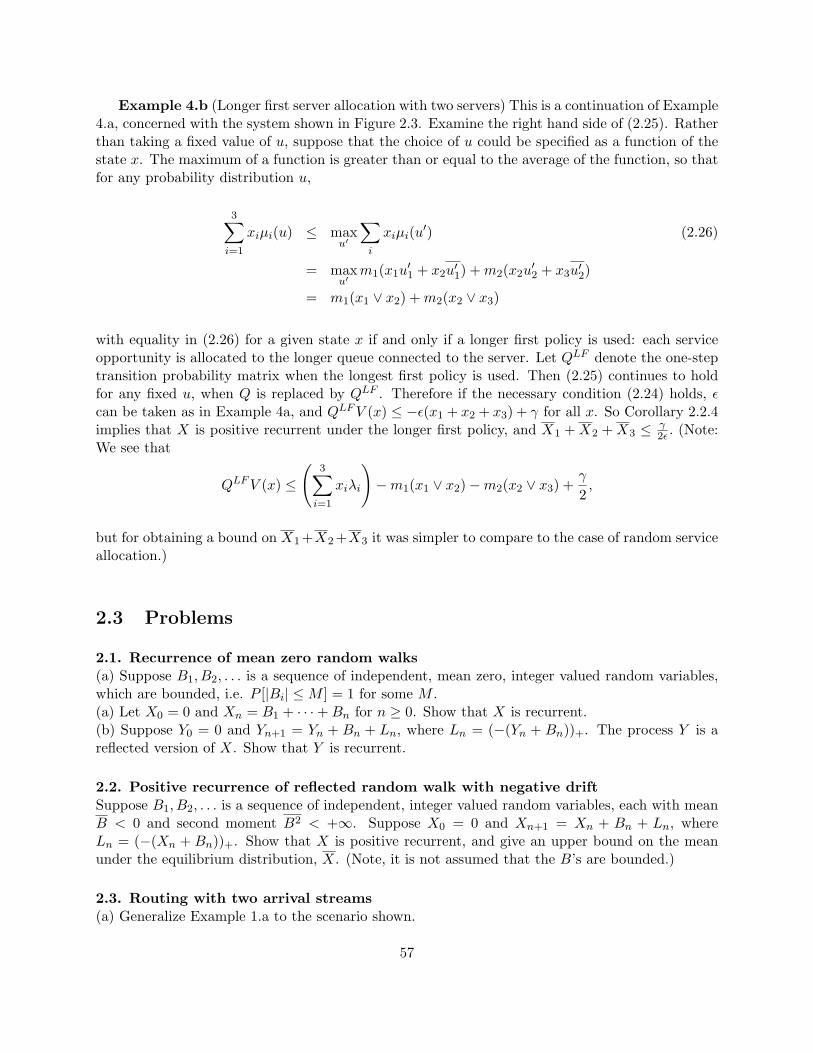
Example 4.b (Longer first server allocation with two servers) This is a continuation of Example4.a, concerned with the system shown in Figure 2.3. Examine the right hand side of (2.25). Ratherthan taking a fixed value of u, suppose that the choice of u could be specified as a function of thestate x. The maximum of a function is greater than or equal to the average of the function, so thatfor any probability distribution u,

3∑i=1

xiµi(u) ≤ maxu′

∑i

xiµi(u′) (2.26)

= maxu′

m1(x1u′1 + x2u′1) + m2(x2u

′2 + x3u′2)

= m1(x1 ∨ x2) + m2(x2 ∨ x3)

with equality in (2.26) for a given state x if and only if a longer first policy is used: each serviceopportunity is allocated to the longer queue connected to the server. Let QLF denote the one-steptransition probability matrix when the longest first policy is used. Then (2.25) continues to holdfor any fixed u, when Q is replaced by QLF . Therefore if the necessary condition (2.24) holds, εcan be taken as in Example 4a, and QLF V (x) ≤ −ε(x1 + x2 + x3) + γ for all x. So Corollary 2.2.4implies that X is positive recurrent under the longer first policy, and X1 + X2 + X3 ≤ γ

2ε . (Note:We see that

QLF V (x) ≤

(3∑

i=1

xiλi

)−m1(x1 ∨ x2)−m2(x2 ∨ x3) +

γ

2,

but for obtaining a bound on X1 +X2 +X3 it was simpler to compare to the case of random serviceallocation.)

2.3 Problems

2.1. Recurrence of mean zero random walks(a) Suppose B1, B2, . . . is a sequence of independent, mean zero, integer valued random variables,which are bounded, i.e. P [|Bi| ≤ M ] = 1 for some M .(a) Let X0 = 0 and Xn = B1 + · · ·+ Bn for n ≥ 0. Show that X is recurrent.(b) Suppose Y0 = 0 and Yn+1 = Yn + Bn + Ln, where Ln = (−(Yn + Bn))+. The process Y is areflected version of X. Show that Y is recurrent.

2.2. Positive recurrence of reflected random walk with negative driftSuppose B1, B2, . . . is a sequence of independent, integer valued random variables, each with meanB < 0 and second moment B2 < +∞. Suppose X0 = 0 and Xn+1 = Xn + Bn + Ln, whereLn = (−(Xn + Bn))+. Show that X is positive recurrent, and give an upper bound on the meanunder the equilibrium distribution, X. (Note, it is not assumed that the B’s are bounded.)

2.3. Routing with two arrival streams(a) Generalize Example 1.a to the scenario shown.

57

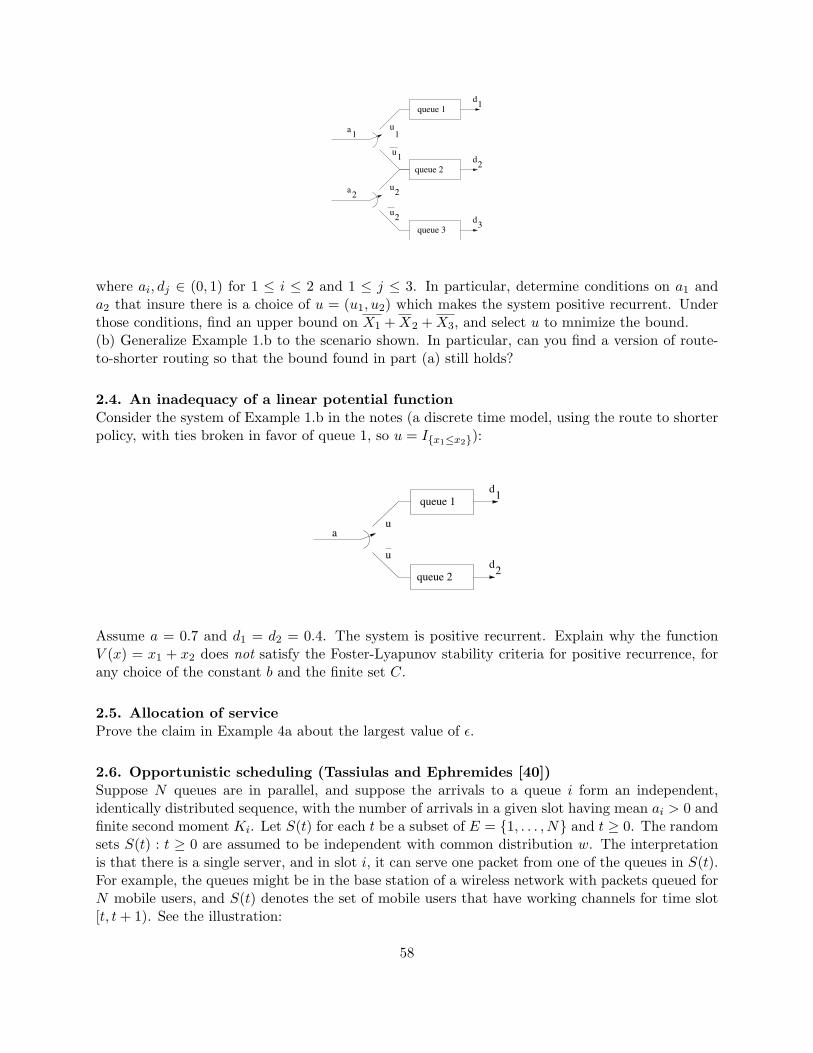
1

queue 1

queue 2 2d

1d

d

1

2

u

u

u

u2queue 3 3

2a

a1

where ai, dj ∈ (0, 1) for 1 ≤ i ≤ 2 and 1 ≤ j ≤ 3. In particular, determine conditions on a1 anda2 that insure there is a choice of u = (u1, u2) which makes the system positive recurrent. Underthose conditions, find an upper bound on X1 + X2 + X3, and select u to mnimize the bound.(b) Generalize Example 1.b to the scenario shown. In particular, can you find a version of route-to-shorter routing so that the bound found in part (a) still holds?

2.4. An inadequacy of a linear potential functionConsider the system of Example 1.b in the notes (a discrete time model, using the route to shorterpolicy, with ties broken in favor of queue 1, so u = Ix1≤x2):

u

queue 1

queue 2 2d

1d

au

Assume a = 0.7 and d1 = d2 = 0.4. The system is positive recurrent. Explain why the functionV (x) = x1 + x2 does not satisfy the Foster-Lyapunov stability criteria for positive recurrence, forany choice of the constant b and the finite set C.

2.5. Allocation of serviceProve the claim in Example 4a about the largest value of ε.

2.6. Opportunistic scheduling (Tassiulas and Ephremides [40])Suppose N queues are in parallel, and suppose the arrivals to a queue i form an independent,identically distributed sequence, with the number of arrivals in a given slot having mean ai > 0 andfinite second moment Ki. Let S(t) for each t be a subset of E = 1, . . . , N and t ≥ 0. The randomsets S(t) : t ≥ 0 are assumed to be independent with common distribution w. The interpretationis that there is a single server, and in slot i, it can serve one packet from one of the queues in S(t).For example, the queues might be in the base station of a wireless network with packets queued forN mobile users, and S(t) denotes the set of mobile users that have working channels for time slot[t, t + 1). See the illustration:

58

state s

queue 11

queue 22

N queue N

a

.

.

.

a

a

Fading

channel

(a) Explain why the following condition is necessary for stability: For all s ⊂ E with s 6= ∅,∑i∈s

ai <∑

B:B∩s 6=∅

w(B) (2.27)

(b) Consider u of the form u = (u(i, s) : i ∈ E, s ⊂ E), with u(i, s) ≥ 0, u(i, s) = 0 if i 6∈ s, and∑i∈E u(i, s) = Is 6=∅. Suppose that given S(t) = s, the queue that is given a potential service op-

portunity has probability distribution (u(i, s) : i ∈ E). Then the probability of a potential serviceat queue i is given by µi(u) =

∑s u(i, s)w(s) for i ∈ E. Show that under the condition (2.27), for

some ε > 0, u can be selected to that ai + ε ≤ µi(u) for i ∈ E. (Hint: Apply the min-cut, max-flowtheorem, given in Chapter 6 of the notes, to an appropriate graph.)(c) Show that using the u found in part (b) that the process is positive recurrent.(d) Suggest a dynamic scheduling method which does not require knowledge of the arrival rates orthe distribution w, which yields the same bound on the mean sum of queue lengths found in part (b).

2.7. Routing to two queues – continuous time modelGive a continuous time analog of Examples 1.a and 1.b. In particular, suppose that the arrivalprocess is Poisson with rate λ and the potential departure processes are Poisson with rates µ1 andµ2.

2.8. Stability of two queues with transfersLet (λ1, λ2, ν, µ1, µ2) be a vector of strictly positve parameters, and consider a system of two servicestations with transfers as pictured.

2

station 1

station 2

u!

2"

" 1 µ 1

µ

Station i has Possion arrivals at rate λi and an exponential type server, with rate µi. In addi-tion, customers are transferred from station 1 to station 2 at rate uν, where u is a constant withu ∈ U = [0, 1]. (Rather than applying dynamic programming here, we will apply the method ofFoster-Lyapunov stability theory in continuous time.) The system is described by a continuous-time Markov process on Z2

+ with some transition rate matrix Q. (You don’t need to write out Q.)(a) Under what condition on (λ1, λ2, ν, µ1, µ2) is there a choice of the constant u such that theMarkov process describing the system is positive recurrent?(b) Let V be the quadratic Lyapunov function, V (x1, x2) = x2

12 + x2

22 . Compute the drift function

QV .

59

(c) Under the condition of part (a), and using the moment bound associated with the Foster-Lyapunov criteria, find an upper bound on the mean number in the system in equilibrium, X1+X2.(The smaller the bound the better.)

2.9. Stability of a system with two queues and modulated serverConsider two queues, queue 1 and queue 2, such that in each time slot, queue i receives a newpacket with probability ai, where 0 < a1 < 1 and 0 < a2 < 1. Suppose the server is described by athree state Markov process, as shown.

queue 2a

a1

2

1

2

0 ! server longer

queue 1

If the server process is in state i for i ∈ 1, 2 at the beginning of a slot, then a potential serviceis given to station i. If the server process is in state 0 at the beginning of a slot, then a potentialservice is given to the longer queue (with ties broken in favor of queue 1). Then during the slot,the server state jumps with the probabilities indicated. (Note that a packet can arrive and departin one time slot.) For what values of a1 and a2 is the process stable? Briefly explain your answer(but rigorous proof is not required).

60

Chapter 3

Queues with General InterarrivalTime and/or Service TimeDistributions

3.1 The M/GI/1 queue

An M/GI/1 queue is one in which the arrival process is memoryless (in fact, Poisson, with someparameter λ > 0), the service times X1, X2, . . . of successive customers are independent with ageneral probability distribution function B, and there is a single server. The number of customersin the system at time t is denoted N(t). A sample path of N is illustrated in Figure 3.1. For ease ofnotation, it is assumed that customers are served in the order in which they arrive. This is knownas the First-Come, First-Served (FCFS) service discipline. As indicated in the figure, we define thefollowing auxiliary variables:

Cn denotes the nth customer

qn is the number in the system just after Cn departs, equilibrium distribution (dk : k ≥ 0)

q′n is the number in the system just before Cn arrives, equilibrium distribution (rk : k ≥ 0)

vn is the number of customers which arrive while Cn is being served

Our goal will be to compute the distribution of N(t) in equilibrium.Note that the random variable N(t) for a fixed time t does not determine how long the customer

in the server (if any) at time t has been in the server, whereas the past history (N(s) : s ≤ t) doesdetermine this time-in-service. The time-in-service of the customer in the server is relevant tothe distribution of the future of the process N , unless the service time distribution is exponential.Thus, unless the service time distribution is exponential, (N(t) : t ≥ 0) is not Markov.

Suppose for now that equilibrium distributions exist. Since the arrivals form a Poisson sequence,the equilibrium distribution of N is the same as the distribution r = (rk) seen by arrivals. Since asmost one arrival and one departure can occur at a time, r = d (see exercise). Thus, rk = pk = dk

for all k.Consider the evolution of (qn : n ≥ 0). Just after Cn+1 begins service, there are qn + Iqn=0

customers in the system. The term Iqn=0 accounts for the arrival of Cn+1 in case the system is

61

Nt

t

qqq 1 3

2

X X X 1 2 3v =2v =3 1 v =0 2 3

Figure 3.1: A typical sample path for an M/GI/1 queueing system

empty upon the departure of Cn. During the period Cn+1 is served, there are vn+1 arrivals. Thisleads to the recursion

qn+1 = qn − Iqn 6=0 + vn+1 (3.1)

The variables vn are independent and identically distributed with common z-transform

V (z) = E[zvn ] =∫ ∞

0

[e−λx

∞∑k=0

(λxz)k

k!

]dB(x) (3.2)

=∫ ∞

0e−λx+λxzdB(x) (3.3)

= B∗(λ− λz), (3.4)

and mean V ′(1) = −λB∗′(0) = λX = ρ. Thus, the sequence (qn : n ≥ 0) is Markov with the onestep transition probability matrix (letting (αk : k ≥ 0) denote the distribution of the vn):

P =

α0 α1 α2 . . .α0 α1 α2 . . .

α0 α1 α2 . . .. . . . . . . . .

. (3.5)

Due to the nearly upper triangular structure of the matrix P it is possible to recursively findthe elements of p as a multiple of p0, and then find p0 at the end by normalizing the sum toone. Another approach is to work with z-transforms, writing the equation p = pP as zP (z) =[P (z) + p0(z − 1)]V (z). Solve this to obtain

P (z) =p0(z − 1)V (z)

z − V (z)(3.6)

To determine the constant p0 use the fact that limz→1 P (z) = 1 (use l’Hospital’s rule and the factV ′(1) = λX = ρ) to obtain p0 = 1− ρ. Therefore,

P (z) =(1− ρ)(z − 1)V (z)

z − V (z), (3.7)

62

which is the celebrated formula of Polleczek and Khinchine for the M/GI/1 system. Computationof the derivatives at one of P (z), again using l’Hospital’s rule, yields the moments Nk of thedistribution of the number in system. In particular,

N = ρ +λ2X2

2(1− ρ). (3.8)

To obtain the mean number in the queue, simply subtract the mean number in the server, ρ. Toobtain the mean waiting time (in queue or system) apply Little’s law to the corresponding meannumber in system. For example, the mean waiting time in the queue is

W =λX2

2(1− ρ). (3.9)

It is remarkable the W depends only on λ, X and X2 = (X)2 +V ar(X). Note that W is increasingin the variance of X, for fixed mean X and arrival rate λ.

A simple alternative derivation of (3.9) is based on renewal theory. Suppose the order of serviceis first-come, first-served. The mean waiting time W of a typical arrival is the same as the meanamount of work in the system at the time of arrival, which by the PASTA property is the sameas the mean amount of work in the system in equilibrium. The mean work in the system can bedecomposed to the mean work in the server plus the mean work in the queue. Thus,

W = R + NQX, (3.10)

where

R = ρ

(X2

2X

), (3.11)

which is the product of the probability the server is busy (ρ) times the mean residual service timeof a customer in service, which is determined by renewal theory. The other term on the right of(3.10) accounts for the portion of delay caused by the customers that are in the queue at the timeof an arrival. Applying Little’s law, NQX = λWX = ρW , substituting into (3.10) and solvingyields W = R/(1− ρ), which is equivalent to the desired formula (3.9).

3.1.1 Busy Period Distribution

Call the customers that arrive during the service interval of a given customer an offspring of thatcustomer. The offspring of a customer, together with the offspring of the offspring, and so forth,is the set of descendants of the customer. The length of the busy period initiated by the firstcustomer is equal to the sum of the service times of the customer itself and of all its descendants.The number of offspring of the first customer is v1, which, given that X1 = x, has the Poissondistribution of mean λx.

The length of the busy period L can be expressed as the sum

L = X1 + L1 + L2 + . . . + Lv1 (3.12)

where X1 is the service time of the first customer in the busy period, v1 is the number of offspringof that customer, and Li is the sum of the service time of the ith offspring of C1 and the service

63

time of that offspring’s descendants. Notice that the joint distribution of L1, L2, . . . , Lv1 is as ifindependent samples with the same distribution as L are drawn.

Condition on X1 to obtain:

G∗(s) = E[e−sL] =∫ ∞

0e−sx

( ∞∑n=0

G∗(s)ne−λx (λx)n

n!

)dB(x) (3.13)

=∫ ∞

0e−sxe−λx+λG∗(s)xB(dx) (3.14)

= B∗(s + λ− λG∗(s)) (3.15)

Obtain g1 = X/(1−ρ). Can also get this by a renewal argument. Obtain also g2 = X2/(1−ρ)3.

3.1.2 Priority M/GI/1 systems

Suppose there are n independent arrival streams, each modeled as a Poisson process, with the ithhaving arrival rate λi. Suppose the streams are merged into a single-server queueing system, andthat the service times of customers from the ith stream are identically distributed with the samedistribution as a generic random variable Xi.

An issue for the system may be the service order. For example, for a pure priority serviceorder, the server attempts to serve the available customer with the highest priority. Some finerdistinctions are possible. If, for example, service of a lower priority customer is interrupted bythe arrival of a higher priority customer, the service discipline is said to be preemptive priority.Otherwise it is nonpreemptive priority.

Does the mean waiting time of a customer (averaged over all the streams according to arrivalrates) depend on the service discipline? The answer is yes, which is why mass service facilities (suchas supermarket checkout lines) often give priority to customers with short service requirements.

The stream obtained by merging the arrival streams is again M/GI/1 type. The arrival rateof the combined stream is λ = λ1 + . . . + λn, and the service time of a customer in the combinedstream is distributed as the random variable X = XJ . Here the index J is chosen at random, withP [J = j] = λj/λ, and J,X1, . . . , Xn are mutually independent. Note that

X =∑

i

λiXi

λand X2 =

∑i

λiX2i

λ(3.16)

As long as customers are served in FCFS order, (3.9) is valid. The PASTA property and the FCFSservice order implies that W is equal to the mean work in the system, where work is measured inunits of time. Therefore,

Mean work in system =λX2

2(1− ρ)=

R

1− ρ. (3.17)

where R is given by (3.11), which here can be written as

R =λX2

2=∑n

i=1 λiX2i

2.

Although (3.17) was just derived under the assumption that the service order is FCFS, the termsinvolved do not depend on the order of service, as long as the server remains busy whenever there

64

is work to be done (in which case the system is said to be “work conserving”). Thus, (3.17) is validfor any work-conserving service discipline.

Assuming the required equilibria exist, the mean work in the queue composed of type i customersis NiXi = λiWiXi = ρiWi for each i, and the mean amount of work in the server is R. The meanwork in the system is thus (

∑ni=1 ρiWi)+R. Equating this with the last expression in (3.17) yields

that

(∑

i

ρiWi) + R =R

1− ρ, (3.18)

which can be simplified to yield the “conservation of work” equation:∑i

ρiWi =ρR

1− ρ. (3.19)

This equation is true for any work-conserving service order for which the required equilibriummeans exist.

In order to derive the mean waiting time of customers of stream i a particular service ordermust be specified. As mentioned above, if the order is FCFS, then the mean waiting time is thesame for all streams, and is given by (3.9). Suppose now that the nonpreemptive priority disciplineis used, with stream i having priority over stream j if i ≤ j. Let Wi continue to denote the meanwaiting time in queue for customers of stream i. Upon arrival to the queue, a customer from stream1 need wait only for the completion of the customer in service (if any) and for the service of otherstream 1 customers, if any, already in the queue. Thus, W1 = R+(λ1W1)/µ1, where by Little’s lawwe write λW1 for the mean number of stream one customers in the queue, and R is the expectedresidual service time of the customer in service, if any:

R =λX2

2=∑n

i=1 λiX2i

2(3.20)

Solving for W1 yields

W1 =R

1− ρ1. (3.21)

Next, argue that W2 is equal to R + (λ1W1)/µ1 + (λ2W2)/µ2 + λ1X1W2. The first three termsin this sum account for the residual service time and the service times of stream 1 and stream 2customers already in the queue at the time of arrival of a stream 2 packet. The last term accountsfor the expected wait due to type 1 customers that arrive while the typical arrival from stream 2is in the queue. Solve for W2 to find

W2 =R + ρ1W1

1− ρ1 − ρ2=

R

(1− ρ1)(1− ρ1 − ρ2)(3.22)

Finally, continuing by induction on i, obtain

Wi =R

(1− ρ1 − . . .− ρi−1)(1− ρ1 − . . .− ρi)(3.23)

for nonpreemptive priority order of service.

65

Nt

tq ’ 2q ’=01

v ’ =0 1 v ’ =0 2 v ’ =2 4

q ’ 3 q ’4

v ’ =0 3

Figure 3.2: A GI/M/1 queue sample path

3.2 The GI/M/1 queue

A GI/M/1 queue is one in which the arrival process is a renewal process, service times are inde-pendent and exponentially distributed with a common mean, and there is a single server. Let Adenote the cumulative distribution function and 1/λ the mean of the interarrival times, and let µdenote the parameter of the service times. The number of customers in the system at time t isdenoted N(t). A sample path of N is illustrated in Figure 3.2. It is assumed that customers areserved in FCFS order.

It is useful to think of the service process as being governed by a Poisson process of rateµ. Jumps in the process denote potential service completions. A potential service completionbecomes an actual service completion if there is at least one customer in the system at the timeof the potential service completion. By the properties of the Poisson process and the exponentialdistribution, this view of the system is consistent with its distribution. Define the following auxiliaryvariables, which are indicated in Figure 3.2:


q′n is the number in the system just before Cn arrives, equilibrium distribution (rk : k ≥ 0)

vn is the number of potential service completions which occur during the interarrival period justbefore the arrival of Cn.

Note that the random variable N(t) for a fixed time t does not determine how long before timet the last customer arrival occurred, whereas the past history (N(s) : s ≤ t) does determine thetime-since-most-recent-arrival. The time-since-most-recent-arrival is relevant to the distribution ofthe future of the process N , unless the interarrival distribution is exponential. Thus, unless thearrival process is Poisson, (N(t) : t ≥ 0) is not Markov. Nevertheless, the mean waiting time, andin fact the waiting time distribution, can be determined by focusing on the process (q′n : n ≥ 1).

Consider the evolution of (q′n : n ≥ 0). Just after Cn arrives, there are q′n + 1 customers in thesystem. There are no more arrivals and potentially as many as q′n departures in the period strictly

66

between arrival times of Cn and Cn+1. Therefore,

q′n+1 = (q′n + 1− vn+1)+ (3.24)

The variables vn are independent and identically distributed with common z-transform A∗(µ−µz). and mean −µA∗′(0) = µ/λ = 1/ρ. Thus, the sequence (q′n : n ≥ 0) is Markov with the onestep transition probability matrix (letting (βk : k ≥ 0) denote the distribution of the vn):

P =

1− β0 β0 0 0 . . .

1− β0 − β1 β1 β0 0 . . .1− β0 − β1 − β2 β2 β1 β0 0 . . .

......

......

. . . . . .

. (3.25)

The equilibrium equation r = rP can be written

rk = β0rk−1 + β1rk + . . . k ≥ 1 (3.26)

Seek a solution of the form rk = (1− σ)σk for some σ > 0. This yields the equation for σ:

σ = A∗(µ− µσ) (3.27)

The function A∗(µ−µσ) is strictly convex, value one and derivative 1/ρ at σ = 1. Thus, a solutionσ with 0 < σ < 1 exists if and only if ρ < 1.

If an equilibrium probability distribution r = (rk : k ≥ 0) of (q′k) exists, then the process ispositive recurrent. Recall from the proof of Proposition 1.7.2, that for a given state, say k, themean number of visits to state k + 1 per excursion from state k is rk+1/rk. Since the process canincrease by only one at a time, in order that the process reach k + 1 before k given that it starts ink, it must take its first jump towards state k + 1. As soon as the process crosses below state k, ithas no more opportunities to hit k + 1 before reaching k. By the shift invariance of the transitionprobabilities, it follows that the ratio rk+1/rk is the same for all k.

rk+1

rk= E[number of visits to k + 1 before return to k|q′0 = k] (3.28)

This ratio does not depend on k. Thus, if any equilibrium distribution exists, it must be a geometricdistribution.

Given q′n = k, the waiting time in queue of Cn is the sum of k independently distributed Poissonrandom variables with parameter µ, which has Laplace transform µ/(µ + s). Thus, the Laplacetransform of the waiting time in equilibrium is

E[e−sW ] = (1− σ)∞∑

k=0

σk

(µ

s + µ

)k

(3.29)

= 1− σ + σ

[µ(1− σ)

s + µ(1− σ)

](3.30)

Thus, the equilibrium waiting distribution is a mixture of the random variable that is identicallyzero, and an exponentially distributed random variable with parameter µ(1 − σ). Thus, P [W >x] = σ exp(−xµ(1 − σ)). and W has mean W = σ/((1 − σ)µ). By Little’s law, the mean numberin the system is given by N = λ(W + 1/µ) = ρ/(1 − σ). The total time in the system, T , canbe represented as T = W + X, where W is the waiting time, X is the service time, and W andX are mutually independent. The Laplace transform of the system time is given by E[e−sT ] =E[e−sW ]E[e−sX ] = (1−σ)µ

s+µ(1−σ) . That is, the total time in the system T is exponentially distributedwith parameter µ(1− σ).

67

3.3 The GI/GI/1 System

A GI/GI/1 queue is one in which the arrival process is renewal type, the service times of successivecustomers are independent and identically distributed, and there is a single server. It is assumedthat customers are served in FCFS order.


xn is the service time required for the nth customer

tn is the time between the arrival of Cn−1 and Cn

wn is the waiting time in queue of the nth customer

U(t) is the work in system, also known as the virtual waiting time, at time t

Take as the intitial condition for the system that it is empty at time 0 and C1 arrives at time t1.With these definitions, notice that wn = U(t1 + . . . + tn−).

A useful stochastic equation is derived next. Just after the arrival of customer Cn, the amountof work in the system is wn + xn, and the work begins to decrease at unit rate. Customer Cn+1

arrives to find the system nonempty if and only if wn + xn − tn+1 > 0, and if this condition holdsthen wn+1 = wn + xn − tn+1. Therefore, in general,

wn+1 = (wn + un)+ (3.31)

where un = xn − tn+1. The random variables of the sequence (un : n ≥ 1) are independent andidentically distributed, because the same is true of the two independent sequences (xn : n ≥ 1) and(tn : n ≥ 1). Then w1 = 0, and by repeated use of (3.31),

wn = max0, wn−1 + un−1= max0, un−1 + max0, wn−2 + un−2= max0, un−1, un−1 + un−2 + wn−2= max0, un−1, un−1 + un−2, un−1 + un−1 + un−2 + wn−3...

...= max0, un−1, un−1 + un−2, . . . , un−1 + . . . u1

Let us next consider the question of stability. Define a random variable wn by

wn = max0, u1, u1 + u2, . . . , u1 + . . . un−1, (3.32)

which is the same as wn, but with the sequence (u1, . . . , un−1) reversed in time. Since time reversalpreserves the distribution of the un sequence, it is clear that for each n, wn has the same distributionas wn.The sequence wn is nondecreasing in n, so that the limit

w∞ = limn→∞

wn

= max0, u1, u1 + u2, . . .

68

exists (with values in (0,∞]) and is equal to the maximum of the partial sums of the un sequence asshown. Since convergence with probability one implies convergence in distribution, it follows thatthe variables (wn) converge in distribution to w∞. Since convergence in distribution is determinedby marginal distributions only, it follows that

lim-in-distn→∞wn = w∞ (3.33)

Suppose that the xn and tn have finite means, so that un also has a finite mean and the stronglaw of large numbers applies: limn→∞(u1+. . .+un)/n = E[u1] with probability one. If E[un] < 0, itfollows that limn→∞(u1+. . .+un) = −∞ with probability one, which implies that P [w∞ < ∞] = 1.The arrival rate is λ = 1/E[t1] and the service rate is µ = 1/E[x1]. Letting ρ = λ/µ as usual,it has just been proved that if ρ < 1, then the variables wn have a limiting distribution with noprobability mass at +∞.

There are techniques for computing the distribution of waiting time. One is based on Wiener-Hopf spectral factorization, and another on certain identities due to F. Sipitzer. However, somesimple bounds on the waiting time distribution, presented in the next section, are often more usefulin applications.

3.4 Kingman’s Bounds for GI/GI/1 Queues

The elegant bounds, due to J.F.C. Kingman, on the mean and tail probabilities for the waitingtime in a GI/GI/1 system are given in this section. Let σ2

z denote the variance of a random variablez.

Proposition 3.4.1 (Kingman’s moment bound) The mean waiting time W for a GI/GI/1 FCFSqueue satisfies

W ≤ λ(σ2x + σ2

t )2(1− ρ)

(3.34)

Proof. Let w denote a random variable with the distribution of w∞ and let u denote a randomvariable independent of w with the same distribution as the un’s. Taking n → ∞ in (3.31) yieldsthat w

d= (w + u)+, where “ d=” denotes equality in distribution. In particular, E[w] = E[(w + u)+]and E[w2] = E[(w + u)2+]. Clearly

w + u = (w + u)+ − (w + u)−, (3.35)

where (w + u)− = −min0, w + u. Taking expectations of each side of (3.35) yields E[u] =−E[(w + u)−]. Squaring each side of (3.35), using the fact (w + u)+(w + u)− = 0 and takingexpectations yields

E[w2] + 2E[w]E[u] + E[u2] = E[(w + u)2+] + E[(w + u)2−],

or equivalently

E[w] =E[u2]− E[(w + u)2−]

−2E[u]

=σ2

u − σ2(w+u)−

−2E[u].

69

Noting that σ2(w+u)−

≥ 0 and σ2u = σ2

x + σ2t yields the desired inequality.

Exercise: Compare Kingman’s moment bound to the exact expression for W in case the inter-arrival times are exponentially distributed. Solution: Then σ2

t = 1λ2 so the bound becomes

E[w] ≤λ(σ2

x + 1λ2 )

2(1− ρ)

whereas by the Polleczek and Khinchine mean formula for an M/GI/1 queuing system

E[w] =λ(σ2

x + 1µ2 )

2(1− ρ).

Next Kingman’s tail bound is given. Let wn denote the waiting time in queue of the nth customerin a GI/GI/1 system. Then wn+1 has the same probability distribution as max0≤k≤n u1+ . . .+uk,where uk is the service time required by the kth customer minus the length of time between thekth and k + 1th arrivals. By assumption, the random variables u1, u2, ... are identically distributed.Suppose E[un] < 0 and that φ(θ) = E[exp(θun)] < +∞ for some θ > 0. Let θ∗ = supθ : φ(θ) ≤ 1.

Proposition 3.4.2 (Kingman’s tail bound) For n ≥ 0 and b ≥ 0, P [wn+1 ≥ b] ≤ exp(−θ∗b).

Proof. Choose any θ > 0 such that φ(θ) ≤ 1. Let M0 = 1 and Mk = exp(θ(u1 + . . . +uk)). Thenthe probability in question can be expressed as P [wn+1 ≥ b] = P [(max0≤k≤n Mk) ≥ exp(θb)]. It iseasy to check that E[Mk+1|Mk, . . . , M0] ≤ Mk, so by Lemma 3.4.3 below,

P [ max1≤k≤n

Mk ≥ exp(θb)] ≤ E[M0]/ exp(θb) = exp(−θb). (3.36)

Thus, P [wn+1 ≥ b] ≤ exp(−θb) for 0 < θ < θ∗, which implies the proposition.

Lemma 3.4.3 Let M0,M1, . . . be nonnegative random variables such that E[Mk+1|Mk, . . . ,M0] ≤Mk for k ≥ 0 (i.e. M is a nonnegative supermartingale). Then for any n ≥ 0, P [(max0≤k≤n Mk) ≥γ] ≤ E[M0]/γ.

Proof. Let τ = mink ≥ 0 : Mk ≥ γ, with the convention that τ = +∞ if the indicated set isempty. Then (max0≤k≤n Mk) ≥ γ if and only if Mτ∧n ≥ γ, where a∧b denotes the minimum of a andb. This fact and the simple “Markov inequality” implies that P [(max0≤k≤n Mk) ≥ γ] = P [Mτ∧n ≥γ] ≤ E[Mτ∧n]/γ. Since E[Mτ∧n] = E[M0] for n = 0, the proof can be completed by showing thatE[Mτ∧n] in nonincreasing in n. To that end, note that Mτ∧(n+1)−Mτ∧n = (Mn+1−Mn)Iτ>n, so

E[Mτ∧(n+1)]− E[Mτ∧n] = E[(Mn+1 −Mn)Iτ>n]= E[E[(Mn+1 −Mn)Iτ>n|Mn, . . . , M0]]= E[E[(Mn+1 −Mn)|Mn, . . . , M0]Iτ>n]≤ 0,

where we use the fact that the event τ > n is determined by M0, . . . , Mn. The lemma is proved.

70

c

F(c)

p

F-1(p)

1

1

Figure 3.3: A distribution function and its inverse

Exercise: Compare Kingman’s tail bound to the exact tail probabilities in case the service timedistribution is exponential. Solution: In that case φ(θ) = µ

µ−θA∗(θ) so the equation for θ∗ becomesA∗(θ) = 1 − θ

µ . With the change of variable θ = µ(1 − σ) this equation becomes the same asthe equation for σ in the analysis of a GI/M/1 queueing system. Thus, θ∗ in Kingman’s boundis equal to µ(1 − σ) where σ is the value determined in the analysis of a GI/M/1 system. Thus,P [w∞ ≥ b] = σ exp(−θ∗b), showing that Kingman’s bound gives the same exponential behavior asthe actual tail probabilities.

3.5 Stochastic Comparison with Application to GI/GI/1 Queues

Before describing the most basic part of the theory of stochastic comparison theory, we shall reviewthe problem of generating a random variable with a given cumulative distribution function. SupposeF is a probability distribution function and that U is a random variable uniformly distributed onthe interval [0, 1]. The inverse function of F is defined by

F−1(p) = supx : F (x) ≤ p (3.37)

and an example is pictured in Figure 3.5. The graph of F−1 is the graph of F reflected aboutthe line of slope one through the origin. Let X = F−1(U). Then for any constant c, P [X ≤ c] =P [F−1(U) ≤ c] = P [U ≤ F (c)] = F (c), so that X has distribution Fc.Exercise 1. a) Find and sketch F−1 assuming that F is the distribution function of an exponentialrandom variable with parameter α. b) Repeat part a) in case F corresponds to a random variableuniformly distributed over the set 1, 2, 3, 4, 5, 6. Simultaneously sketch F and F−1 as is done inFigure 3.5. Is F−1 right-continuous? c) Show that if F (c) ≤ G(c) for all c, then F−1(p) ≥ G−1(p)for all p.

Definition 3.5.1 Let F and G be two distribution functions. We say F stochastically dominatesG, and write F G, if F (c) ≤ G(c) for all constants c. If X and Y are two random variables,we say that X stochastically dominates Y , and write X Y , if FX stochastically dominates FY ,where FX is the distribution function of X and FY is the distribution function of Y .

71

Note that whether X Y , depends only on the individual distributions of X and Y , andotherwise does not depend on the joint distribution of X and Y . In fact, X and Y don’t even needto be random variables on the same probability space.

The fundamental proposition of stochastic comparison theory is the following:

Proposition 3.5.2 X Y if and only if there is a pair of random variables (X, Y ) defined onsome probability space such that the following three conditions hold:

Xd= X (the notation “ d=” means the variables have the sam probability distribution.)

Yd= Y

P [X ≥ Y ] = 1.

Proof. If X Y , let U be a uniform random variable and let X = F−1X (U) and Y = F−1

Y (U).Then (X, Y ) satisfies the required three conditions.

Conversely, if there exists (X, Y ) satisfying the three conditions then for any constant c, theevent X ≤ c is a subset of the event Y ≤ c (possibly ignoring an event of probability zero).Therefore, FX(c) = FX(c) ≤ FY (c) = FY (c), so that indeed X Y .

A useful method for deriving bounds on probability distributions, called the stochastic compar-ison method, or coupling method, consists of applying Proposition 3.5.2. Note that the randomvariables X and Y may have little to do with each other. They may be independent, or even definedon different probability spaces. Variables X and Y defined on a common statespace, with X

d= X

and Yd= Y are called coupled versions of X and Y . Thus, to establish that X Y , it suffices to

show the existence of coupled versions X and Y such that P [X ≥ Y ] = 1.

Example Let wn, for n ≥ 1, denote the sequence of waiting times for the customers in aGI/GI/1 queue, which is empty at the time of arrival of customer one. Then the random variablesw1, w2, . . . defined by (3.32) are coupled versions of w1, w2, . . .. Since the random variables wn arenondecreasing in n with probability one, conclude that w1 ≺ w2 ≺ · · · . That is, the waiting timeof customer Cn stochastically increases with n.

Example As a related example, let us demonstrate that the waiting time in a GI/GI/1 queueis an increasing function of the service time distribution in the sense of stochastic comparison.That is, suppose there are two queueing systems, called system 1 and system 2. Suppose that bothsystems are initially empty and that the sequence of arrival times of the two systems have identicaldistributions. Suppose that both systems use the FIFO service order and that the service times ofthe customers in system i, (i = 1 or i = 2) are independent and identically distributed with CDFB(i). Let W

(i)n denote the waiting time of the nth customer in system i.

Suppose that B(1) B(2). We will establish that for each n, W(1)n W

(2)n . Consider a probabil-

ity space on which there is defined a sequence of variables (T1, T2, . . .) which has the same distribu-tion as the sequence of interarrival times for either of the two queuing systems being compared. Onthe same probability space, for each n, let (X(1)

n , X(2)n ) be a pair of random variables such that X

(1)n

has CDF B(1), X(2)n has CDF B(2), and P [X(1)

n ≥ X(2)n ] = 1. Such a pair can be constructed accord-

ing to Proposition 3.5.2. Moreover, the pairs in the sequence (X(1)n , X

(2)n ))n≥1 can be constructed

72

to be mutually independent, and also to be independent of (T1, T2, . . .). For i = 1 or i = 2, defineW

(i)n to be the waiting time of the nth customer in the queueing system in which (T1, T2, . . .) is the

interarrival time sequence and (B(i)1 , B

(i)2 , . . .) is the sequence of customer service times. Clearly

W(i)n and W

(i)n have the same distribution, so it suffices to prove that P [W (1)

n ≥ W(2)n ] = 1. How-

ever, the fact W(1)1 = W

(2)1 = 0, the update equations W

(i)n+1 = (W (i)

n − Tn+1 + X(i)n )+, and the fact

P [X(1)n ≥ X

(2)n ] = 1 imply that P [W (1)

n ≥ W(2)n ] = 1 for all n ≥ 1 by induction on n. Applying

Proposition 3.5.2 again, we conclude that W(1)n W

(2)n for all n, as advertised.

Execise 2 a) Show that X Y if and only if for every nondecreasing function φ, E[φ(X)] ≥ E[φ(Y )].(Another type of stochastic ordering requires the inequality to hold only for convex, nondecreasingfunctions φ.) b) Let X be uniformly distributed on [0,1], let Y be exponentially distributed withE[Y ] = 1, and let Z have the Poisson distribution with E[Z] = 1. Identify any stochastic orderingsthat appear between pairs of these random variables (e.g., is X Y ?). c) Suppose X Y andE[X] = E[Y ]. Prove that X and Y have the same distribution.

3.6 GI/GI/1 Systems with Server Vacations, and Application toTDM and FDM

In a GI/GI/1 system with server vacations, whenever the server finishes serving a customer orreturns from a vacation, and finds the system empty, the server goes on another vacation. Avacation is a period of time in which the server does not serve customers, even if one or morecustomers arrive during the period. An effective method for accounting for the effect of vacationsis to compare the sample paths of a system operating without vacations to one with vacations. Thefollowing variables will be used.

• won is the waiting time in queue of the nth customer in the system without vacations.

• wn is the waiting time in queue of the nth customer in the system with vacations.

• t1 is the time of the first arrival and, for n ≥ 1, tn+1 is the time between the nth and n + 1th

arrivals. These variables are used in both systems. The variables t1, t2, . . . are assumed tobe independent and identically distributed.

• xn is the service time required by the nth customer. These variables are used in both systems.The variables x1, x2, . . . are assumed to be independent and identically distributed.

• Vn is the length of the nth vacation period for the system with vacations. The variables Vn

for n ≥ 1 are assumed to be independent, and identically distributed.

The two systems both start empty, and in the system with vacations, the server initiates avacation at time zero with duration V0. Roughly speaking, the main difference between the twosystems is that when the nth customer begins service in the system with vacations, the total idletime of the server is of the form V0 + . . . + Vk for some k. In fact, k is the minimum integer,subject to the constraint that the idle time in the system with vacations is greater than or equal tothe idle time in the system without vacations. This idea is expressed concisely in the lemma below.

Let γ(u) denote the residual lifetime process for the renewal process determined by V0, V1, . . . .That is, γ(u) = V0 + . . . + Vl(u) − u, where l(u) = mink : V0 + . . . + Vk ≥ u. Also, let Io

n

73

denote the total idle time, in the system without vacations, up to the time the nth customer begins(or ends) service.

Lemma 3.6.1 For n ≥ 1,wn = won + γ(Io

n).

Proof. Argue by induction on n. Since w1 = γ(Io1) and wo

1 = 0, the lemma is true for n = 1.Suppose the lemma is true for n, and argue that it is true for n + 1 as follows. Let x denote theamount of time (possibly zero) the server in the system without vacations is idle between servicesof the nth and n + 1th customers. Therefore, Io

n+1 = Ion + x, and two cases are considered: (1) If

x ≤ wn − won then then the server in the system with vacations will not take a vacation between

service of the nth and n + 1th customers. Therefore wn+1 − won+1 = wn − w0

n − x = γ(Ion) − x =

γ(Ion + x) = γ(Io

n+1), as was to be proved. (2) If x > wn − won then at the time of arrival of the

n + 1th customer, both systems are empty and both have been idle for Ion+1 time units. Therefore,

wn+1 = γ(Ion+1) and wo

n+1 = 0, so again wn+1 − won+1 = γ(Io

n+1). The induction step is complete,and the lemma is proved.

By renewal theory, if the distribution of V1 is nonlattice type, the random variable γ(u) convergesin distribution as u →∞, where the limit has probability density function (p.d.f.) fγ given by

fγ(c) =P [V1 ≥ c]

E[V1]. (3.38)

It is useful to skip the question of convergence to equilibrium by choosing the distribution of V0

to make (γ(u) : u ≥ 0) a stationary random process (rather than only asymptotically stationary).Thus, assume that V0 has p.d.f. fγ . Consequently, γ(u) has distribution function fγ for all u ≥ 0.Since (γ(u) : u ≥ 0) is independent of (wo

n, Ion), the conditional density of γ(Io

n) given (won, Io

n) isagain fγ . Thus (wo

n, Ion) and γ(Io

n) are mutually independent. The following proposition is proved.

Proposition 3.6.2 Suppose V0 has p.d.f. fγ. Then won and γ(In

o ) are independent, γ(Ino ) has p.d.f.

fγ, and wn = won + γ(Io

n).

Since the kth moment of a random variable with p.d.f. fγ is mk+1/((k + 1)m1 where mj = E[V j1 ],

the following corollary is immediate from the Proposition.

Corollary 3.6.3 Suppose V0 has p.d.f. fγ. Then E[wn] = E[won] + m2/(2m1) and Var(wn) =

Var(won) + m3/(3m1)− (m2/(2m1))2.

If V0 has some arbitrary distribution, the Proposition still holds in a limiting sense, under anadditional assumption to prevent periodic behavior. For example, if E[x1] < E[t1] < ∞ and if V1

or x1− t1 is nonlattice type, then the pair (γ(Ion), wo

n) converges in distribution as n →∞, and thelimit (γ, w) has independent coordinates, with the first having p.d.f. fγ .

As an example, one can model a time-slotted system in which the time axis is divided intoframes of length M , for some constant M , and service can only begin at the beginning of a frame.To that end, choose the service time random variable x1 to be a possibly-random integer multipleof M , and suppose that the vacations are all M units in duration. Then fγ is the uniform densityon the interval [0,M ]. By the corollary, the mean waiting time in the system is M/2 time unitslarger than the mean waiting time in the system with the same service time distribution, withoutthe constraint that service begin at the beginning of frames.

74

Continuing this example further, if M is an integer, we can think of a frame as being composedof M unit length slots. The waiting time in the slotted system is the same as that for a streamtraversing a Time Division Multiplexed (TDM) communication link, in which the stream is servedduring one slot per frame. In the TDM system there are M arrival streams, all multiplexed onto asingle line, and the queuing processes for the M streams are not related. When the vacations aredropped, the model represents a Frequency Division Multiplexed (FDM) communication link of thesame total capacity. In an FDM multiplexed link, the M streams again do not interact. The meanwaiting times are thus related by WTDM = WFDM + M/2. However, for the TDM system, theactual service time of a packet is M − 1 time units less than the service time in an FDM system, sothe total mean system time for packets in the two systems are related by TTDM = TFDM−M/2+1.Note that there is not much difference between the delay in TDM and FDM systems, especially forheavily loaded systems.

Finally, to specialize the example further, if the traffic arrival process is Poisson with rate λ/Mpackets/slot and if each packet is served in M slots in the FDM system and in one slot in the TDMsystem (with only one out of every M slots being available), then the FDM system is an M/GI/1system with constant service times (i.e. an M/D/1 system). The P-K mean formula thus yieldsWFDM = λM/(2(1− λ)), and so WTDM = WFDM + M/2 = M/(2(1− λ)).

3.7 Effective Bandwidth of a Data Stream

There has been an extensive effort since the inception of packet-switched communication networksto characterize the traffic carried by networks. The work aims to account for the bursty nature ofmany data sources. This section describes one approach for defining the effective bandwidth of adata stream. The approach is based on the theory of large deviations.

Recently, there has been a keen interest in accounting for the observations of many studies oftraffic in real networks, which indicate that traffic streams exhibit self-similar behavior. That is,the random fluctuations in the arrival rate of packets appears to be nearly statistically the sameon different time scales, ranging over several orders of magnitude. We touch on this developmentbriefly in the context of the effective bandwidth of a self-similar Gaussian source. An extensiveannotated bibliography on the subject is given in [43].

One of the primary goals of information theory is to identify the “effective information rate”of a data source. The entropy or the rate-distortion function of a data source may be thought ofas such. The theory of effective bandwidth, described in this section, has a similar goal. Anotherconnection between the theory of effective bandwidth of data streams and information theory isthat much of the theory of effective bandwidth is based on large deviations theory, which is a closecousin to Shannon’s theory of information. Moreover, there is possibly some yet to be discovereddirect connection between the theory of effective bandwidth and Shannon’s theory of information.For example, perhaps an “effective-bandwidth vs. distortion” function can be computed for somenontrivial sources.

A major way that the theory of effective bandwidth differs from the Shannon theory is that ittreats the flow of data bits as it would the flow of anything else, such as a fluid. The values of thebits are not especially relevant. The idea is that individual connections or data streams carried by anetwork may be variable in nature. The data rate may be variable in a statistical sense, in that therate produced by the stream or connection is not a priori known and can possibly be considered tobe random. It may also be varying in time: such is the case for data streams produced by variable

75

rate source coders. Suppose many variable data streams are multiplexed together onto a line witha fixed capacity, where capacity is measured in bits per second. Because of statistical multiplexing,the multiplexer has less work to do than if all the data streams were sending data at the peak rate allthe time. Therefore a given data stream has an effective bandwidth (which depends on the context)somewhere between the mean and peak rate of the stream. The use of the word “bandwidth” in thephrase “effective bandwidth” has a different meaning than that commonly used by radio engineers.A better name might be “effective data rate.” However, the name “effective bandwidth” is alreadydeeply entrenched in the networking literature, so is used here.

To illustrate the ideas in the simplest setting first, we begin by considering a bufferless com-munication link, following Hui [20, 21]. The total offered load (measured in bits per second, forexample) is given by

X =J∑

j=1

nj∑i=1

Xji (3.39)

where J is the number of connection types, nj is the number of connections of type j, and Xji is thedata rate required by the ith connection of type j. Assume that the variables Xji are independent,with the distribution of each depending only on the index j. If the link capacity is C then theprobability of overload, P [X > C], can be bounded by Chernoff’s inequality:

log P [X ≥ C] ≤ log E[es(X−C)] = s(J∑

j=1

njαj(s)− C) (3.40)

where αj(s) is given by

αj(s) =1s

log E[esXji ]. (3.41)

Thus, for a given value of γ, the quality of service constraint log P [X > C] ≤ −γ is satisfied if thevector n = (n1, . . . , nJ) lies in the region

A = n ∈ RJ+ : min

s>0[s(

J∑j=1

njαj(s)− C)] ≤ −γ = ∪sA(s) (3.42)

where

A(s) = n ∈ RJ+ :

J∑j=1

njαj(s) ≤ C − γ

s. (3.43)

The complement of A relative to RJ+ is convex. Let n∗ be on the boundary of A (think of n∗ as

a “nominal” value of the vector n). A polyhedral subset of A, delineated by a hyperplane tangentto the boundary of A at n∗, is given by A(s∗), where s∗ achieves the minimum in (3.42). Thus, anyvector n ∈ ZJ

+ satisfyingJ∑

j=1

njαj(s∗) ≤ C − γ

s∗(3.44)

satisfies the quality of service constraint. Once C, γ, and s∗ are fixed, the sufficient condition (3.44)is rather simple. The number αj(s∗) is the effective bandwidth of a type j connection, and C−γ/s∗ isthe effective capacity. Condition (3.44) is analogous to the condition in classical information theory

76

which insures that a particular channel is capable of conveying several independent data sourceswithin specified average distortions, namely that the sum of the rate distortion functions evaluatedat the targeted distortions should be less than or equal to the channel capacity.

As long as the random variables Xji are not constant, the function αj is strictly increasing,and ranging from the mean, E[Xji] as s → 0, to the peak (actually the essential supremum,supc : P [Xji > c] > 0), of Xji. Note that the effective bandwidth used depends on the variables∗. Such dependence is natural, for there is a tradeoff between the degree of statistical multiplexingutilized and the probability of overload, and the choice of the parameter s∗ corresponds to selectinga point along that tradeoff curve. Roughly speaking, as the constraint on the overflow probabilitybecomes more severe, a larger value of s∗ is appropriate. For example, if γ is very large, thenthe sets As are nonempty only for large s, so that the choice of s∗ is also large, meaning that theeffective bandwidths will be near the peak values.

The set A defined in (3.42) is only an inner bound to the true acceptance region for the constraintlog P [X > C] ≤ −γ. However, if C and γ both tend to infinity with their ratio fixed, then thetrue acceptance region, when scaled by dividing by C, converges to A scaled by dividing by C [23].(The scaled version of A depends only on the ratio of C to γ.) This follows from Cramer’s theorem(see [36]), to the effect that Chernoff’s bound gives the correct exponent.

So far, only a bufferless link confronted with demand that is constant over all time has beenconsidered. The notion of effective bandwidth can be extended to cover sources of data which varyin time, but which are statistically stationary and mutually independent [3, 37, 7]. Let Xji[a, b]denote the amount of traffic generated by the ith connection of type j during an interval [a, b]. Weassume that the process X is stationary in time. Set

αj(s, t) =1st

log E[esXij [0,t]]. (3.45)

For t fixed, the function αj is the same as the one-parameter version of αj considered above,applied to the amount of work generated in an interval of length t. Beginning with the well-knownrepresentation of Loynes for the stationary queue length, Q(0) = supt≥0 X[−t, 0]− tC, we write

log P [Q(0) > B]= log P [sup

t≥0X[−t, 0]− tC > B] (3.46)

∼ supt≥0

log P [X[−t, 0]− tC > B] (3.47)

∼ supt≥0

mins≥0

stJ∑

j=1

njαj(s, t)− s(B + tC)

(3.48)

The symbol “∼” used in (3.47) and (3.48) denotes asymptotic equivalence of the logarithms ofthe quantities on either side of the symbol. The use of this symbol is justified by limit theoremsin at least two distinct regimes: (1) the buffer size B tends to infinity with n and C fixed, and(2) the elements of the vector n, the capacity C, and the buffer space B all tend to infinity withthe ratios among them fixed. Under either limiting regime, the line (3.47) is justified by the factthat the probability of the union of many rare events (with probabilities tending to zero at variousexponential rates) is dominated by the probability of the most probable of those events. Theline (3.48), which represents the use of the Chernoff bound as in (3.40), relies on the asymptotic

77

exactness of the Chernoff bound (Cramer’s theorem or more general large deviations principles suchas the Gartner-Ellis theorem. See [36]).

Equations (3.46)-(3.48) suggest that the effective bandwidth to be associated with a connectionof type j is αj(s∗, t∗), where t∗ achieves the supremum in (3.48), and s∗ achieves the minimum in(3.48) for a nominal value n∗ of n. The approximate condition for meeting the quality of servicerequirement log P [Q(0) > B] ≤ −γ for n near n∗ is then

J∑j=1

njαj(s∗, t∗) ≤ C +B

t∗− γ

s∗t∗

This region scales linearly in γ if n∗, B and C scale linearly in γ, and asymptotically becomesa tight constraint as γ → ∞. The value t∗ is the amount of time that the system behaves in anunusual way to build up the queue length just before the queue length exceeds B. The quantityC + B/t∗ − γ/s∗t∗ is the effective capacity of the link. Following [35], we call t∗ the critical timescale. In the first limiting regime, described above, t∗ tends to infinity, so the effective bandwidthbecomes αj(∞, s∗). Use of the Gartner-Ellis theorem of large deviations theory allows the limittheorems in the first limiting regime to be carried out for a wide class of traffic streams withmemory.

The above approximation simplifies considerably in the case that the traffic process is Gaussian.In particular, suppose also that there is only one class of customers (so we drop the index j and letn denote the number of connections) and that for each i the traffic Xi(0, t] is Gaussian with meanλt and variance V (t). The corresponding effective bandwidth function is α(s, t) = λ + sV (t)/2t.Inserting this into (3.48) and then performing the minimization over s yields that

log P [Q(0) > B] ∼ −n inft

((c− λ)t + b)2

2V (t)(3.49)

where b is the buffer space per connection (so B = nb) and c is the capacity per connection (C = nc).Suppose V (t)/t2H converges to a finite constant σ2 as t tends to infinity, where H, known as the

Hurst parameter, typically satisfies 1/2 ≤ H < 1. If H = 1/2, we see the process does not exhibitlong range dependence. In particular, if X has independent increments (therefore the increments ofa Brownian motion with drift λ and diffusion parameter σ2), then V (t) = σ2t and moreover (3.49)holds with exact equality.

If H > 1/2 (but still H < 1) then the critical time scale t∗ is still finite. That is, even in thepresence of long range dependence, the critical time scale is still finite in the limiting regime of C,B and n tending to infinity with fixed ratios among them [35]. The value of V (t) for t larger thant∗ therefore does not influence the approximation.

See [11] and [23] for extensive surveys on effective bandwidth, and [43] for a very extensivebibliographic guide to self-similar traffic models and their use. The paper [4] presents significantbounds and analysis related to notions of equivalent bandwidth with a different terminology. Fi-nally, the paper [22] connects the theory of effective bandwidths to thermodynamics and statisticalmechanics.

3.8 Problems

3.1. A queue with customers arriving in pairsCustomers arrive at a single-server queue two at a time. The arrival instants for pairs of customers

78

are given by a Poisson process with rate λ. The service times of customers are independent,exponentially distributed with parameter µ. Let N(t) denote the number of customers in thesystem at time t. (a) The process (N(t) : t ≥ 0) is a continuous time pure jump Markov processwith statespace Z+. Sketch the transition rate diagram of N . (b) See what can be deduced aboutN by applying the Foster-Lyapunov stability criteria and related moment bounds for the Lyapunovfunction V (x) = x. (c) Repeat part (b) using V (x) = x2

2 .(d) Solve for the z transform of the equilibrium distribution and find the equilibrium distribution.Under what condition does it exist (i.e. under what condition is N positive recurrent?)(e) Let (rk : k ≥ 0) and (dk : k ≥ 0) be the equilibrium probabilities defined by

rk = P [there are k in the system just before the arrival of a pair of customers]dk = P [there are k in the system just after the departure of a typical customer].

Express (rk : k ≥ 0) and (dk : k ≥ 0) in terms of (pk : k ≥ 0), λ and µ. In particular, does rk = pk?or dk = pk? or rk = dk?

3.2. Token bucket regulation of a Poisson streamA token bucket traffic regulation scheme works as follows. The packet stream to be regulated ismodeled as a Poisson stream with arrival rate λ. There is a token pool that holds up to B tokens.When a packet arrives, if there is a token in the token pool then the packet instantly passes throughthe regulator, and one of the tokens is removed from the token pool. If instead the token pool isempty, then the packet is lost. (Notice that packets are never queued.) New tokens are generatedperiodically, with one time unit between successive generation times. If a token is generated whenthe token pool is full, the token is lost. (The token pool acts like a ”leaky bucket”.) (a) Identify anembedded discrete-time, discrete-state Markov process, and describe the one-step transition prob-abilities of the chain. (b) Express the fraction of packets lost (long term average) in terms of λ, Band π, where π denotes the equilibrium probability vector for your Markov chain. (You do NOTneed to find π.) (c) As an approximation, suppose that the times between new token generationsare independent, exponentially distributed with common mean 1. Find a fairly simple expressionfor the loss probability.

3.3. Extremality of constant interarrival times for G/M/1 queuesConsider two G/M/1 queueing systems with common service rate µ. The first has a general in-terarrival distribution function A(t) with mean 1/λ such that λ/µ < 1. The second has constantinterarrival times, all equal to 1/λ. (Thus the interarrival distribution function in the second sys-tem is Ad(t) = 0 if t < 1/λ and Ad(t) = 1 otherwise, and the system is called a D/M/1 system).(a) Show that the Laplace transforms are ordered: A∗

d(s) ≤ A∗(s) for all s ≥ 0. (b) Show thatthe mean number in the system at arrival times (in equilibrium) and the mean waiting time in thesystem is smaller for the D/M/1 system.

3.4. Propagation of perturbationsConsider a single-server queueing system which is initially empty and for which a total of fivecustomers arrive, at times 1,2,5,13, and 14, respectively. Suppose the amounts of time required toserve the customers are 5,2,4,2,2 time units, respectively. (a) Sketch the unfinished work in thesystem as a function of time. Indicate the departure times of the five customers, and compute thewaiting times in queue of the five customers. (b) Repeat part (a), assuming that the service time

79

of the second customer is increased to 3 time units. (c) Repeat part (a), assuming the service timeof the second customer is increased to 4 time units. (d) Describe briefly in words how in generalan increase in service time of one customer effects the waiting times of other customers in the system.

3.5. On priority M/GI/1 queuesConsider an M/GI/1 system with preemptive resume priority service. There are assumed to be twopriority classes, with independent arrival streams and service requirements. Class 1 has priorityover class 2. Customers of the ith class arrive according to a Poisson process of rate λi, and theservice times of customers of class i are independent and identically distributed. Use Xi to denotea random variable with the same distribution as the service requirements for class i, for i = 1 ori = 2. (a) Describe what “preemptive resume priority” means. (b) Derive the mean time in thesystem, T1 and T2, for class 1 and class 2, respectively.

3.6. Optimality of the µc ruleConsider an M/G/1 queue with customer classes 1 through K and a nonpreemptive priority ser-vice discipline. Let µi = 1/Xi where Xi denotes the mean service time for type i customers andlet ci, with ci > 0, denote the cost per unit time of holding a class i customer in the queue. Forsome permutation σ = (σ1, σ1, . . . , σK) of (1, 2, . . . ,K), the class σ1 customers are given the highestpriority, the class σ2 customers are given the next highest priority, and so on. The resulting longrun average cost per unit time is

∑i λiciWi(σ), where Wi(σ) is the mean waiting time of class i

customers under the priority order σ. (a) Show that an ordering σ minimizes the long-run aver-age cost per unit time over all possible orderings if and only if µσ1cσ1 ≥ µσ2cσ2 ≥ . . . ≥ µσK cσK .(Hint: If σ does not satisfy the given condition, then for some i, µσicσi < µσi+1cσi+1 . Appeal to theconservation of work equation to argue that by swapping σi and σi+1, an ordering σ with strictlysmaller cost than σ is obtained. You still also need to figure out how to prove both the “if” and“only if” portions of the statement.) (b) Write a brief intuitive explanation for the result of part (a).

3.7. A queue with persistent customersConsider a queue with feedback as shown, where λ, D > 0 and 0 ≤ b ≤ 1. New arrivals occuraccording to a Poisson process of rate λ. The service time of a customer for each visit to thequeue is the constant D. Upon a service completion, the customer is returned to the queue withprobability 1− b.

D!

1!b

b

(a) Under what condition is the system stable? Justify your answer.(b) Suppose the service order is FIFO, except that a returning customer is able to bypass all othercustomers and begin a new service immediately. Denote this by PR, for priority to returning,service order. Express the mean total system time of a customer, from the time it arrives untilthe time it leaves the server for the last time, in terms of λ, b, and D. (Hint: A geometricallydistributed random variable with parameter p has first moment 1

p and second moment 2−pp2 .)

(c) If instead the service within the queue were true FIFO, so that returning customers go to theend of the line, would the mean total time in the system be larger, equal, or smaller than for PRservice order? Would t

80

he variance of the total time in the system be larger, equal, or smaller than for PR service order?

3.8. A discrete time M/GI/1 queueConsider a single server queue in discrete time. Suppose that during each time slot, one customerarrives with probability p, and no customers arrive with probability 1 − p. The arrival events fordifferent slots are mutually independent. The service times are independent of the arrival timesand of each other, and the service time of any given customer is equally likely to be 1,2,3,4,5 or 6slots. Find W , the mean number of complete slots spent in the queue by a typical customer (don’tinclude time in service). Show your reasoning. Also identify an embedded Markov chain for thesystem.3.9. On stochastic ordering of sampled lifetimesLet f and g be two different probability density functions with support R+, and with the samefinite mean, m1. Let fL and gL denote the corresponding sampled lifetime densities: fL(x) = xf(x)

m1

and gL(x) = xg(x)m1

. Show that it is impossible that fL ≺ gL. (We write fL ≺ gL to denote that arandom variable with pdf fL is stochastically smaller than a random variable with pdf gL. Notethat the mean of fL does not have to equal the mean of gL.)

3.10. Effective bandwidth, bufferless linkConsider a bufferless link of fixed capacity C = 200 serving connections of 2 types. The data rate ofeach connection is random, but constant in time. The data rate required by a connection of type 1is uniformly distributed over [0,2], the data rate required by a connection of type 2 is exponentiallydistributed with mean 1, and requirements for different connections are mutually independent. (a)Calculate the effective bandwidth functions α1(s) and α2(s). (b) Find the largest integer n so thatthe Chernoff inequality implies that the blocking probability is less than or equal to 0.001 for anominal load of n connections of each type. Show your work for full credit! (Hint: Write a shortcomputer program for this problem. For a given value of n the Chernoff bound is computed by aminimization over s. Then n can be adjusted by binary search – increasing n if the correspondingoverflow probability is too small, and decreasing n if the corresponding overflow probability is toolarge.) (c) Compute the effective bandwidths α1(s∗), α2(s∗), and the effective capacity C+ log(0.001

s∗ .Which of the two effective bandwidths is larger? Sketch the corresponding acceptance region A(s∗).Here s∗ denotes the optimizing value of s in the Chernoff bound. (Hint: The nominal load point(n,n) should be contained in the region A(s∗). Which of the two effective bandwidths is larger?)

3.11. Effective bandwidth for a buffered link and long range dependent Gaussian traf-ficConsider a link with buffer size B = 100 and fixed capacity C = 200, serving connections of 2types. The amount of data offered by a connection of type i over an interval of length t is assumedto be Gaussian with mean t and variance Vi(t) = t2Hi , where Hi is the Hurst parameter. AssumeH1 = 0.5 and H2 = 0.9. (So the class 2 connections have long-range dependence.) (a) Computethe largest value n so that the Chernoff approximation for the overflow probability for n connec-tions of each type (simultaneously) is less than or equal to exp(−γ) = 0.001. (Hint: Write a shortcomputer program for this problem. For a given value of C and t the approximation is computedby a minimization over s, which can be done analytically. The maximization over t can be donenumerically, yielding the approximate overflow probability for the given value of C. Finally, C canbe adjusted by binary search as in the previous problem. Also, compute the effective bandwidths

81

α1(s∗, t∗), α2(s∗, t∗), the critical time t∗, and the effective capacity Ceff = C + Bt∗ −

γs∗t∗ . Sketch

the corresponding acceptance region A(s∗, t∗). (Hint: The nominal load point (n, n) should becontained in the region A(s∗, t∗). Which of the two effective bandwidths is larger?) (b) Redoproblem (a) for overflow probability exp(−γ) = 0.00001. and comment on the differences betweenthe answers to parts (a) and (b).

3.12. Extremal equivalent bandwidth for fixed mean and rangeSuppose X is a random variable representing the rate of a connection sharing a bufferless link.Suppose the only information known about the probability distribution of X is that E[X] = 1 andP [0 ≤ X ≤ 2] = 1. For a given s > 0 fixed, what specific choice of distribution of X meeting theseconstraints maximizes the equivalent bandwidth α(s), where α(s) = ln(E[esX ])

s ?

82

Chapter 4

Multiple Access

4.1 Slotted ALOHA with Finitely Many Stations

Suppose M stations wish to communicate to each other via a shared broadcast channel. Supposethat time is divided into equal length slots such that the length of each slot is the amount of timeneeded for a station to transmit one packet of information.

Consider a particular station and a particular time slot. If the station does not have a packetat the beginning of the slot, then it receives a new packet in the slot with probability qa. A newpacket (one that arrives in the slot) cannot be transmitted in the slot. If the station already has apacket to transmit at the beginning of the slot, then it transmits the packet with probability qx inthe slot, and the station is not eligible to receive any new packets in the slot. The events of packetarrival and transmission at the different stations are mutually conditionally independent, given thestatus of the stations at the beginning of the slot.

If no station transmits a packet in the slot, the channel is said to be “idle” during the slot, and iftwo or more stations transmit during the slot, a “collision” is said to occur. If either the slot is idleor a collision occurs in the slot, then no packet is successfully transmitted. If exactly one stationtransmits a packet in the slot, then that transmission is called a “success,” and the packet leavesthe system. The station making the successful transmission is eligible to receive a new packet inthe next time slot, while all other stations with packets carry their packets over to the next slot.

The parameters of the model are thus M, qa and qx. Several aspects of the model involvechoices that were made largely for simplicity and tractability. For example, we might have alloweda station to continue receiving packets, even after it already had one to send. However, in somesystems the successful transmission of the first packet in a queue at a station is the most crucial,because that packet can reserve slots (possibly on another channel) for the packets in queue behindit. Also implicit in the model is that a station can determine by the beginning of the next slotwhether its transmission is successful, so that it knows whether to transmit the same packet again,or to switch back to the mode of receiving a new packet. One way to modify the current modelto account for a delay of, say, R time slots would be to time-interleave R independent versions ofthe system. On the other hand, for networks of small physical size, feedback comes so soon thatan unsuccessful transmission can be stopped well before the whole packet is transmitted. That isthe idea of collision detect.

A final aspect of the model we should comment on is that new packets are treated the sameway as packets that have already been transmitted. An alternative is to transmit a new packet

83

with probability one in the first slot after it arrives, and if such transmission is not successful thenthe packet should be retransmitted with probability qr in subsequent slots, until it is successfullytransmitted. Thus, we have adopted a delayed first transmission (DFT) rather than immediate firsttransmission (IFT) model. The qualitative behavior and exact analysis of the two types of modelsare similar. The IFT model can lead to lower mean delays for lightly loaded systems. On the otherhand, the DFT model is less sensitive to variations in the statistics of the arrival process.

Quantities of interest include the mean throughput and mean delay of the system. Since thestations are interchangeable in the model, the process (N(k) : k ≥ 0) is a Markov process, whereN(k) is the number of stations with packets at the beginning of a slot k. Given N(k) = n, theconditional probability of a successful transmission in slot k, PS(n, qx), is given by PS(n, qx) =nqx(1 − qx)n−1, and the conditional probability that there are j arrivals is b(M − n, qa, j), whereb() is the binomial mass function

b(M − n, qa, j) =

(

M − nj

)qja(1− qa)M−n−j 0 ≤ j ≤ M − n

0 else.

Furthermore, whether there is a successful transmission is conditionally independent of the numberof new arrivals, given N(k) = n. Thus, the one step transition probabilities of the process can beexpressed as follows.

P [N(k + 1) = n + i|N(k) = n] = PS(n, qx)b(M − n, qa, i + 1) + (1− PS(n, qx))b(M − n, qa, i)

The equilibrium probability distribution π of the Markov process (N(k)) can be easily computednumerically by matrix iteration. The mean number of packets in the system and mean throughputare given by N =

∑Mn=0 nπn and S =

∑Mn=0 πnPS(n, qx) = (M −N)qa respectively, and by Little’s

law the mean delay is N/S.The dynamical behavior of the system can be better understood by considering the drift of the

random processes (N(k)). The drift at instant k is defined to be E[N(k + 1) − N(k)|N(k)]. It isa function of N(k), and is equal to the expected change in N over slot k, given N(k). Since thechange in N is the number of arrivals minus the number of departures, the drift can be expressedas d(N(k)) where d(n) = (M − n)qa − PS(n, qx).

It is convenient to think of the function d(n) as a one-dimensional vector field. For convenience,consider d(n) for real values of n between 0 and M . The zeros of d(n) are called equilibrium points,and an equilibrium point is called stable if d(n) makes a down-crossing at the equilibrium point.We expect that the sample paths of the Markov process spend much of their time near the stableequilibrium points of (N(k)). If qx is sufficiently small for given values of M and qa, then there isonly a single equilibrium point, which is stable. However, for some parameter values there can bethree equilibrium points, two of which are stable. One of the stable points occurs for a large value ofn, corresponding to large delay and small throughput, whereas the other equilibrium point occursfor a much smaller value of n. The existence of stable equilibrium points at undesirable values ofn indicates the following potential problem with the operation of the system: for a long periodof time the system may stay near the desirable stable equilibrium point, but due to occasionallarge stochastic fluctuations it may move to near the undesirable point. A drastic, and undesirablequalitative change in the performance of the stochastic system can occur rather suddenly.

In many dynamical systems, a control mechanism based on feedback can be used to eliminateundesirable stable equilibrium points. That method is investigated for the ALOHA system in thenext two sections.

84

4.2 Slotted ALOHA with Infinitely Many Stations

No Control

Let Ak denote the number of new packets to arrive in slot k. Assume that the random variables(Ak : k ≥ 0) are independent, identically distributed with E[Ak] = λ and V ar(Ak) < ∞. Forexample, Ak might have a Poisson distribution, which arises in the limit as the number of stationstends to infinity with the aggregate rate of traffic generation set to λ. Suppose that each stationwith a packet at the beginning of a slot transmits in the slot with probability qx. If there are nsuch stations then the probability of a success, PS(n, qx), is given by PS(n, qx) = nqx(1 − qx)n−1.Since limn→∞ PS(n, qx) = 0, there is an no so large that PS(n, qx) ≤ λ/2 for n ≥ no.

We shall argue that this implies that P [limk→∞N(k) = ∞] = 1. Conditioned on the eventN(k) ≥ no, the increment N(k + 1) − N(k) is stochastically greater than or equal to 1 a randomvariable u, where u = A1 − B, and B is a random variable independent of A1 such that P [B =1] = λ/2 = 1 − P [B = 0]. Note that E[u] = λ/2 > 0. Moreover, given N(k) ≥ no, the futureincrements of N are all stochastically larger than u until, if ever, the backlog becomes smallerthan no. Furthermore, there is a positive probability that the backlog will never again be less thanno, because of the following fact: If u1, u2, . . . are independent, identically distributed randomvariables with E[ui] > 0, then P [mink≥1 u1 + . . . + uk ≤ −1] < 1 (otherwise the Strong Law ofLarge Numbers would be violated). Thus, conditioned on the event N(k) ≥ no, there is a positiveprobability that the backlog will converge to infinity and never again cross below no. Since thebacklog must lie above no infinitely often, it follows that P [limk→∞N(k) = +∞] = 1.

Centralized (Unrealistic) Control

It is easy to show that for n fixed, PS(n, qx) is maximized by qx = 1/n, that PS(n, 1/n) = (1 +1/(n − 1))−(n−1) > e−1 and that limn→∞ PS(1, 1/n) = e−1. We can try to apply this result to acollision access system as follows. Let N(k) denote the number of stations with packets to transmitat the beginning of slot k, and suppose that each such station transmits its packet in the slot withprobability 1/N(k). Then if N(k) is not zero, the conditional probability of a successful transmissionin the slot given N(k) is greater than e−1. Thus the delay in the system is no larger than that fora discrete time M/M/1 bulk-arrival system in which the service times are geometrically distributedwith parameter e−1. (The two processes can be constructed on the same probability space so thatthe M/M/1 bulk system always has at least as many packets in it as the ALOHA system.) Themean delay will thus be finite if λ < e−1 and the variance of the number of arrivals in each slot isfinite. Unfortunately, this retransmission procedure is far from being practical because it requiresthat all the stations be aware of the number of stations with packets.

Decentralized Control

The stations can implement a practical variation of the centralized control scheme by estimating thenumber of stations with packets. Suppose, for example, that immediately after slot k the stations

1“Stochastically greater than or equal to” refers to the notion of stochastic comparison, discussed in Section3.5.

85

learn the value of Z(k), where

Z(k) =

0 if the slot was idle1 if there was a successful transmission in the slote if there was a collision in the slot.

The actual number of packets in the system evolves according to the equation

N(k + 1) = N(k)− IZ(k)=1 + A(k), (4.1)

where A(k) is the number of packets to arrive during slot k. By definition the term IZ(k)=1 isone if Z(k) = 1 and zero otherwise, and the stations learn the value of the term because theyobserve Z(k). On the other hand A(k) is independent of N(k) and all the feedback up to andincluding Z(k). Thus, a reasonable way for the stations to update an estimate N(k) of N(k) is bythe following update equations:

N(k + 1) = (N(k)− IZ(k)=1 + c(Z(k)))+ + λ, (4.2)

where c = (c(0), c(1), c(e)) is to be chosen so that the estimator error D(k) defined by D(k) =N(k) − N(k) will tend to remain small for all k. Combining the equations for N(k + 1) andN(k+1), we see that if N(k) > 1−minc(0), c(1), c(e), then D(k+1) = D(k)−(A(k)−λ)+c(Z(k)).Suppose that all stations with a packet to transmit at the beginning of slot k transmit in the slotwith probability min(1, 1/N(k)). The drift of (D(k)) during slot k is given by

E[D(k + 1)−D(k)|N(k), N(k)] =c(0)P [Z = 0|N(k), N(k)] + c(1)P [Z = 1|N(k), N(k)] + c(e)P [Z = e|N(k), N(k)].

It is not hard to show that if either N(k) or D(k) are sufficiently large then

P [Z = 0|N(k), N(k)] ≈ exp(−G(k)),P [Z = 1|N(k), N(k)] ≈ G(k) exp(−G(k)),P [Z = e|N(k), N(k)] ≈ 1− (1 + G(k)) exp(−G(k)).

where

G(k) =

N(k)

ˆN(k)if N(k) 6= 0

0 if N(k) = 0.

Therefore, the drift of D satisfies

E[D(k + 1)−D(k)|N(k), N(k)] ≈ d(G(k)),

whered(G) = c(0) exp(−G) + c(1)G exp(−G) + c(e)(1− (1 + G) exp(−G)).

We would like the sign of the drift of D(k) to be opposite the sign of D(k), in order that the errordrift towards zero. Now D(k) is positive if and only if N(k) is too large (i.e. larger than N(k)),which means that G(k) is less than one. Hence we want to choose the constants (c(0), c(1), c(e))so that d(G) < 0 when G < 1. Similarly we want d(G) > 0 when G > 1. By continuity this forcesd(1) = 1. Since we have only one equation (and two other conditions) for the three constants there

86

0 2 4 6 8 10 12 14 16 18 200

2

4

6

8

10

12

14

16

18

20

n

Estim

ate

of n

Figure 4.1: Drift field for ALOHA with distributed control.

is some flexibility in choosing the constants. One suitable choice is c(0) = −(e−2)/(e−1) ≈ −0.418,c(1) = 0 and c(e) = 1/(e − 1) ≈ 0.582. To summarize, with this choice of (c(0), c(1), c(e)), if thestations use the update formula (4.2) and transmit with probability 1/N(k) in slot k when theyhave a packet, then the estimator error D(k) will tend to drift to zero.

As a check on our calculations we can easily do an exact calculation of the drift vector field ofthe Markov process (N(t), N(t)), given by

d(n, n) = E

[(N(k + 1)−N(k)N(k + 1)− N(k)

)∣∣∣∣ ( N(k)N(k)

)=(

nn

)].

This vector field is plotted in Figure 4.2 for λ = 0.20 and the above value of c.The system should perform almost as well as the system with centralized control. The following

proposition shows that the system with decentralized control is stable for the same arrival rates λas the system with centralized control.

Proposition 4.2.1 Suppose (c(0), c(1), c(e)) are chosen so that d(G) < 0 if G < 1 and d(G) > 0if G > 1. Suppose E[Ak] = λ < e−1, and suppose for some constants a and b, that P [Ak ≥ x] ≤a exp(−bx) for all x > 0. Finally, suppose the system begins in the initial state N(0) = N(0) = 0.Then there exist positive constants A and B with B < 1 so that, for all k, P [N(k) ≥ n] ≤ ABn.

4.3 Bound Implied by Drift, and Proof of Proposition 4.2.1

Proposition 4.2.1 will be proved in this section by a general method which we call the Lyapunovmethod of stochastic stability. The idea is to apply bounds implied by drift analysis (explainednext) to a one-dimensional process which is a function of the main process under study. The

87

function mapping the original process into the one dimensional process is called the Lyapunovfunction. The method offers slick proofs, but, in typical applications, a good understanding of theoriginal process and why it is stable, is needed in order to construct the Lyapunov function.

Bounds Implied by Drift Analysis

Let Y0, Y1, . . . be a sequence of random variables. The drift at instant k is defined by E[Yk+1 −Yk|Y0, Y1, . . . , Yk]. Note that this drift is itself random, being a function of Y0, . . . , Yk. For notationalconvenience, we shall write Fk instead of Y0, Y1, . . . , Yk when conditioning on these variables. Thus,the drift is E[Yk+1−Yk|Fk]. If the sequence Y0, Y1, . . . is a Markov sequence, then the drift at instantk is a function of Yk alone.

Let a be a constant with −∞ ≤ a < ∞, and let εo, λ and D be strictly positive finite constants.Consider the following conditions on the random sequence:

Condition C.1 The drift at instant k is less than or equal to −εo whenever Yk ≥ a, for k ≥ 0.Equivalently, 2

E[(Yk+1 − Yk + εo)IYk≥a|Fk] ≤ 0 k ≥ 0.

One might expect that Condition C.1 alone is enough to guarantee that Yk, at least for largevalues of k, does not tend to be much larger than the constant a (if a is finite) or that Yk tendsto −∞ in some sense as k → ∞ (if a = −∞). However, an additional condition is needed (seehomework exercise). It is sufficient that the increments of the sequence not be too large. That isthe rough idea of Condition C.2:

Condition C.2 There is a random variable Z with E[exp(λZ)] = D so that

P [|Yk+1 − Yk| ≥ x |Fk] ≤ P [Z ≥ x] x > 0.

Let c, η and ρ be constants such that

c ≥ E[exp(λZ)]−(1+λE[Z])λ2

0 < η ≤ λ,η < εo/c and,

ρ = 1− εoη + cη2.

Then ρ < 1 and D ≥ 1, and it is not difficult to show that Conditions C.1 and C.2 imply ConditionD.1, stated as follows:

Condition D.1 E[exp(η(Yk+1 − Yk))IYk≥a|Fk] ≤ ρ for k ≥ 0.Also, Condition C.2 directly implies condition D.2, stated as follows:Condition D.2 E[exp(η(Yk+1 − a))IYk<a|Fk] ≤ D for k ≥ 0.

Proposition 4.3.1 Conditions D.1 and D.2 (and therefore also Conditions C.1 and C.2) implythat

P [Yk ≥ b|Y0] ≤ ρk exp(η(Y0 − b)) +1− ρk

1− ρD exp(−η(b− a)). (4.3)

2The inequality should be understood to hold except possibly on a set of probability zero, because conditionalexpectations are only defined up to events of probability zero.

88

Note that the first term on the right-hand side of (4.3) tends to zero geometrically fast ask → ∞, and the second term tends to zero exponentially fast as b → ∞. Note also in the specialcase Y0 ≤ a that (4.3) yields P [Yk ≥ b|Y0] ≤ D exp(−η(b−a))

1−ρ .Proof. Note that E[exp(ηYk+1)|Y0] = E[E[exp(ηYk+1)|Fk]|F0]. However

E[exp(ηYk+1)|Fk] = E[exp(η(Yk+1 − Yk))IYk≥a|Fk] exp(ηYk)+ E[exp(η(Yk+1 − a))IYk<a|Fk] exp(ηa)

≤ ρ exp(ηYk) + D exp(ηa),

so thatE[exp(ηYk+1)|Y0] ≤ ρE[exp(ηYk)|Y0] + D exp(ηa). (4.4)

Use of (4.4) and argument by induction on k yields that

E[exp(ηYk)|Y0] ≤ ρk exp(ηY0) +1− ρk

1− ρD exp(ηa).

Combining this inequality with the simple Chernoff bound,

P [Yk ≥ b|Y0] = P [exp(ηYk) ≥ exp(ηb)] ≤ exp(−ηb)E[exp(ηYk)|Y0],

establishes (4.3).

Proof of Proposition 4.2.1

In this section we explain how to prove Proposition 4.2.1 by applying Proposition 4.3.1. The driftof the backlog at instant k, (given the state of the system), is E[N(k + 1) − N(k)|N(k), N(k)].If this drift were less than some fixed negative constant whenever N(k) is sufficiently large, thenProposition 4.3.1 could be directly applied to prove Proposition 4.2.1. By comparison with thecentralized control scheme, we see that the drift is negative if the estimate N(k) is close enoughto N(k). It is possible that N(k) is not close to N(k) (so that N(k) itself doesn’t have negativedrift), but in that case the estimation error should tend to decrease.

To turn this intuition into a proof, let Yk = V (N(k), N(k)) where V (n, n) = n+φ(|n−n|) with

φ(u) =

u2

K if 0 ≤ u ≤ K2

2Ku−K3 if u > K2.

for some positive constant K to be specified later. Here V is the Lyapunov function which we useto convert the problem of establishing stability for the two dimensional process (N(k), N(k)) intothe problem of establishing stability for a one dimensional process. Thus, we argue that if K issufficiently large, then the random sequence (Yk) satisfies Conditions C.1 and C.2 for some finiteconstants a, εo, λ, and η, and conditioning on Fk means conditioning on ((N(j), N(j)) : 0 ≤ j ≤ k).Observe that Yk = N(k) + φ(|N(k)−N(k)|) so that the drift of Yk is the sum of the drift of N(k)and the drift of φ(|N(k)−N(k)|). To prove that Condition C.1 holds, note that if Yk is large, and if|N(k)−N(k)| is small, then Yk inherits negative drift from N(k), and the drift of φ(|N(k)−N(k)|)is small because the function φ is nearly flat near zero. On the other hand, if Yk is large, and if|N(k)−N(k)| is also large, then Yk inherits large negative drift from φ(|N(k)−N(k)|). Thus, in

89

either case, when Yk is large it has negative drift, so Condition C.1 is satisfied. Details are left tothe reader. Condition C.2 is easily established–a key point is that the derivative of the function φis bounded by 2K, so

|Yk+1 − Yk| ≤ (2K + 1)|N(k + 1)−N(k)|+ 2K|N(k + 1)− N(k)| (4.5)

Thus, Proposition 4.3.1 can be applied to (Yk : k ≥ 0), and since N(k) ≤ Yk, Proposition 4.2.1follows immediately.

4.4 Probing Algorithms for Multiple Access

The decentralized control strategy described above has obvious deficiencies. For example, if a col-lision is observed, then until there is a success, it is clear that there are at least two backloggedstations. The update procedure would need a larger state space to take advantage of such infor-mation. One could imagine each station computing the conditional distribution of the number ofbacklogged stations, using a Bayesian update formula at each step (in fact this is described inthe paper of A. Segall). This would be realizable if the state space is truncated to a finite set ofstates for the purpose of the estimator. Some approximate equations motivated by this procedurewere given by Rivest. However, a key observation is that any given individual station knows notonly the feedback information, but it also knows the times that it itself transmitted in the past.This information can serve to distinguish the station from other stations, thereby helping to re-solve conflicts. Algorithms called “probing algorithms” or “tree algorithms” take advantage of thisadditional information.

First the basic collision resolution algorithm (CRA) is described. It operates in discrete timewith the same 0−1−e feedback model considered for controlled ALOHA. Suppose there are initiallyk stations with packets to transmit. In the first slot, all stations transmit. If k=0 or k = 1, thenat the end of the slot it is clear that all packets are successfully sent. If k=2 then a collision occursin the first slot.

After a collision, all transmitters involved flip a fair coin with possible outcomes 0 or 1. Thosethat obtain a 0 from their coin flip (those ”flipping 0” for short) retransmit in the very next slot,and those flipping 1 retransmit in the first slot after the algorithm is done processing the groupof stations that flipped a 0. An example involving four stations with packets, A,B, C and D, ispictured in Figure 4.2. Suppose after the initial collision that stations B and C flip 0. Then bothB and C transmit in the second slot, causing another collision. If then C flips 0 and B flips 1, thenC and B are transmitted successfully in the third and fourth slots respectively. After the fourthslot, the stations with packets A and D realize it is time to transmit again, resulting in a collisionin the fifth slot, and so on.

The progress of the algorithm can be traced on a binary tree, as pictured in Figure 4.3. Eachnode of the tree corresponds to a single slot of the algorithm. Each terminal node of the treeconstructed is labeled either 0 or 1, whereas each nonterminal node is labeled e. The algorithmcorresponds to a virtual stack, as pictured in Figure 4.4. Packets all initially enter the top level,called level 0, of the stack. All packets at level 0 at the beginning of a slot are transmitted. If thereis only one packet at level 0, it is thus successfully transmitted. If there are two or more packetsat level 0, then all such packets flip a fair coin, and those that flip 0 stay at level 0 for the nextslot, and all those that flip 1 move down to level 1. A packet that is in any other level l at thebeginning of a slot is not transmitted in the slot. At the end of the slot the packet moves to level

90

l + 1 if there is a collision in the slot, and moves to level l− 1 if there is no collision (i.e. either notransmission or a success) in the slot. For actual implementation of the algorithm, a station witha packet maintains a single counter to keep track of the level of the packet in the virtual stack.

The basic CRA is now completely described. Some comments are in order. First, whenever thereis a collision followed by an idle slot, the next slot will be a collision. For example, the outcomes ofslots 5 and 6 in the example insure that slot 7 will be a collision. Consequently, the CRA can be“improved” by skipping a step in the algorithm. However, this improvement can lead to instabilityif the model assumptions are slightly violated—see problem XXX. Another observation is that allpackets can sometimes be successfully transmitted a slot or more before the algorithm is complete.In the example, the algorithm requires eleven slots, even though all four packets are transmittedin ten slots. The eleventh slot is necessary in order for all stations listening to the channel outputsto learn that the algorithm is indeed complete.

Let Ln denote the mean number of slots needed for a CRA to process a batch of n packets.Then L0 = L1 = 1. To find Ln for n ≥ 2, the outcome of the first slot is to be considered. Then,

Ln = 1 +n∑

k=0

(n

k

)2−nE[additional slots required|k stations flip 0 after first slot]

= 1 +n∑

k=0

(n

k

)2−n(Lk + Ln−k)

= 1 + 2n∑

k=0

(n

k

)2−nLk.

Observing that Ln appears on the right side with a coefficient 2−(n−1), we can solve for Ln yieldingthe recursion:

Ln =1 + 2

∑n−1k=0

(nk

)2−nLk

1− 2−(n−1)(4.6)

Let τ denote the (random) completion time given the number of packets has a Poisson distri-bution with mean µ. The mean of τ can be computed numerically using the expression

τ =∞∑

n=0

µne−µLn

n!.

A more direct way is to note that

τ = E[number of nodes of tree visited]= 1 + 2E[number of nodes corresponding to collisions]

= 1 + 2∞∑

k=0

2kP [a given node in level k of full binary tree corresponds to a collision]

= 1 + 2∞∑

k=0

2k1− (1 + µ2−k) exp(−µ2−k)

The final sum converges quickly, as can be seen from the fact that 1− (1+ ε) exp(−ε) = ε2/2+o(ε2)as ε → 0. Thus, τ is finite for any µ > 0.

91

4.4.1 Random Access for Streams of Arrivals

So far a method for arranging for transmissions of a fixed group of stations with packets hasbeen described. This collision resolution algorithm can be used as a building block to construct arandom access strategy for a continuous stream of arrivals of new packets. In one method, packetsjust arriving are first transmitted in the first slot after the batch in progress has been handled. Thisleads to large variations in batch size. Analysis can be based on the observation that the sequenceof consecutive batch sizes forms a Markov process. A second method, known as continuous entry, isdiscussed in Problem xxx. A third method, known as the decoupled window strategy, is discussedin the next subsection.

4.4.2 Delay Analysis of Decoupled Window Random Access Scheme

Under the decoupled window random access scheme, packets are grouped into batches. The kth

batch consists of those packets that arrive during the time interval [(k − 1)4, k4), where 4 isa parameter of the algorithm. Note that the distribution of the number of packets in a batch isPoisson with mean λ4. Packets in each batch are processed by a separate run of the basic collisionresolution algorithm. The processing time of the kth batch is denoted τk. The variables τk,k ≥ 0are independent and each has the same distribution as the completion time τ of the basic CRAwhen the number of packets involved has the Poisson distribution with mean µ = λ4. Processingof the kth batch begins in the first slot after the (k − 1)th batch is processed, or in the first slotafter time k4, whichever is later.

Let Uk denote the waiting time of the kth batch, which is the amount of time from k4 untilprocessing for batch k begins. Note that for suitable initial conditions, Uk = Uo

k + γk, where γk isuniform on the interval [0,1], and Uo

k is the waiting time of the kth batch in a modified system whichdoes not have time slotting of the transmission process (cf. section on servers with vacations). Thesequence (Uo

k : k ≥ 1) satisfies the equations:

Uok+1 = (Uo

k −4+ τk)+,

which is identical to the update equations for the waiting times in a GI/GI/1 queue (more specif-ically, a D/GI/1 queue), if the τk represent the service times in the GI/GI/1 queue, and if theinterarrival times are the constant 4. For E[Uk] to be bounded as k → ∞ it is necessary andsufficient that τ and V ar(τ) be finite. In fact, by Kingman’s first moment bound,

E[Uok ] ≤ λ(V ar(δ) + V ar(4))

2(1− τ/4)=

λVar(τ)2(1− τ/4)

if the load ρ = τ/4 is less than one. It can be shown that τ has finite variance for any 4 > 0 bymodifying either of the two methods used to compute τ .

For E[Uok ] to be bounded it is thus sufficient that λ < λ4/τ = µ/τ , where µ = λ4. For the

basic CRA, the maximum throughput is maxµ µ/τ = 0.429. ZZZ CHOICE OF 4. It is 0.462 forthe modified CRA.

The maximum throughput can be further increased by terminating the processing of a batchwhenever the conditional distribution of the number of remaining packets is Poisson distributed.Those packets can be regrouped with packets arriving during a different time interval with lengthadjusted so that the mean number of packets in the resulting batch is adjusted to an optimal value.This leads to maximum throughput 0.4872. Finally, with this restart idea used, the tree is no longer

92

symmetric, so further improvement can be gained by adjusting the bias of the coin used, yieldingmaximum throughput 0.4878.

4.5 Problems

(I haven’t assigned these problems recently, and solutions are not provided for them in the back.-BH)4.1. M/G/1 queue with bulk arrivalsConsider a single server queueing system in which customers arrive in batches. Suppose that batchesarrive according to a Poisson process of rate λ, and suppose that P [a batch has k customers]=gk,independently of the time of arrival and of the size of all other batches. Suppose the service timesof all customers are independent with distribution function B(x) and mean 1/µ, and suppose thesequence of service times is independent of the arrival process. Suppose that the customers areserved in FCFS order, and that the customers within a batch are served in some random order thatis independent of the service times of the customers. Think of a “typical” customer as one drawn atrandom from among the first N customers, all choices being equally likely, where N is very large.”// (a) Define the waiting time of a batch to be the length of time from when the batch arrives untilsome customer in the batch begins service. Under what condition is the limiting batch waitingtime finite? Under such condition, what is the mean waiting time of a batch in equilibrium? (Hint:reduce to consideration of an M/G/1 system).(b) What is the distribution of the total number of customers in the same batch as a typicalcustomer? Given that a typical customer is in a batch of size n, what is the conditional distributionof the number, X, of customers in the same batch as the typical customer which are served beforethe customer itself is served? What is the unconditional probability distribution of X? What isE[X]? Double check your answers for the case g1 = g2 = 0.5.(c) What is the mean waiting time in queue for a typical customer?(d) (Effect of statistical multiplexing). If the arrival rate is doubled to 2λ, if the batch sizes havethe same distribution, and if the service times are cut in half, how does the mean waiting time inthe queue change? How about the mean waiting time in the system?(e) (Effect of increasing burstiness). If the arrival rate is halved to λ/2, if the batch sizes aredoubled, and if the service times are kept the same, how does the mean waiting time in the queuechange?4.2. Basic ALOHAConsider a basic ALOHA system with M stations, each having buffer size one, as discussed inclass. (a) Suppose the arrival probability per slot at an empty station is qa = 1/(Me), and that thetransmission probability per slot at an occupied station is qx = 1/M . Perform a drift analysis ofthe system. How many equilibrium points are there? Assuming M is large and approximating themean number of busy stations using drift analysis, derive the throughput and the mean delay. (b)Continue to assume that M is large. Also assume that qx = 3/M and qa = a/M for some constanta. For what value of a is T ≈ M/2 (in other words, about the same as for TDMA), where the meandelay T is again predicted by drift analysis. How many equilibrium points are there for this valueof a?4.3. Basic ALOHA for finite MConsider a slotted ALOHA system with M stations, each with an infinite buffer. Each stationwhich, at the beginning of a slot, has at least one packet, transmits a packet with probability

93

qx. In addition, each station, whether transmitting or not, receives a packet during a slot withprobability qa. Suppose the stations have unbounded buffers. At the end of each slot, all stationslearn how many packets were transmitted. If exactly one is transmitted, that packet leaves thesystem. Otherwise, no packets leave the system. (a) Identify a Markov chain describing the systemand give the one-step transition probabilities. (Hints: What is the state space? To gain intuition,it might help to think about the case M = 2 first.) (b) What is a necessary and sufficient conditionfor the system to be stable? (Be as explicit as possible. You should explain your reasoning but youneedn’t prove your answer.)

4.4. Drift analysis for two interacting Markov queuesConsider a system with two queueing stations. Suppose the arrival processes to the two stationsare independent Poisson processes with the rates λ1 and λ2. Suppose the stations are correlatedin the following sense. When there are n1 customers in the first station and n2 customers in thesecond station, than the instantaneous service rate in the first station is µn1/(n1 + n2) and theinstantaneous service rate in the second station is µn2/(n1 + n2). That is, the effort of a rate µexponential server is allocated among the two stations in proportion to their numbers of customers.a) Sketch the drift vector field of the Markov chain (N1, N2) assuming that λ1 = 1, λ2 = 2 andµ = 4. b) Find the mean total number in the system in equilibrium. c) Under what conditions onλ1, λ2 and µ is the Markov chain positive recurrent? Can you prove your answer?

4.5. Is negative drift alone enough?Let X1, X2, . . . be independent random variables with P [Xk = −2k2] = 1/k2 and P [Xk = 1] =1− 1/k2. Let Yk = X1 + X2 + ... + Xk. (a) Find dk(n) = E[Yk+1 − Yk|Y1, . . . , Yk−1, Yk = n]. Whatdoes your answer suggest about the asymptotic behavior of the sequence (Yk : k ≥ 1)? (b) LetAk be the event Xk = −2k2. Since the sum P [A1] + P [A2] + . . . is finite, the Borel-Cantellilemma implies that P [Ak occurs for infinitely many k] = 0. What does this fact imply about theasymptotic behavior of the random sequence (Yk : k ≥ 1)? (Does the discrepancy between youranswers to (a) and (b) contradict any results from class?)

4.6. Controlled ALOHAConsider a discrete-time controlled ALOHA system. Suppose that just before slot one there areno packets in the system. The number of new packets that arrive during each slot has the Poissondistribution with mean λ, and each new packet arrives at an empty station (infinite user model).The numbers of arrivals during distinct slots are mutually independent. Each station keeps trackof a counter. We use C(k) to denote the (common) value of the counters at the beginning of slotk. We assume C(1) = 0 and use the following update rule: C(k) = (C(k) − 1)+ if no packets aretransmitted in slot k, and C(k) = C(k) + 1 if at least one packet is transmitted in slot k. Supposethat any station with a packet at the beginning of slot k transmits it with probability f(k), wheref(k) = 1/C(k) if C(k) ≥ 1 and f(k) = 1 otherwise.(a) Identify a Markov chain describing thesystem and write down the transition probabilities. (b) For what range of λ is the Markov chainpositive recurrent? (Hint: When the backlog is large, what does the mean number of packetstransmitted per slot drift towards?)

4.7. A controlled ALOHA systemConsider a discrete-time controlled ALOHA system, as discussed in class. Suppose that just beforeslot one there are no packets in the system. The number of new packets that arrive during eachslot has the Poisson distribution with mean λ, and each new packet arrives at an empty station(infinite user model). The numbers of arrivals during distinct slots are mutually independent. Each

94

station keeps track of an estimate N(k) as follows:

N(k + 1) = (N(k)− IZ(k)=1 + c(Zk))+ + e−1

where (c(0), c(1), c(e)) = (−0.418, 0, .582). (If the e−1 here were replaced by λ, this would beidentical to the estimator considered in class. The estimator here does not require knowledge ofλ.) Suppose that any station with a packet at the beginning of slot k transmits it with probabilitymin(1/N(k), 1). (a) Identify a Markov chain describing the system, and write down the transitionprobabilities. (b) When N(k) and N(k) are both large, the difference GoN(k)−N(k) drifts towardszero for some value of Go. How is the constant Go determined? (Be as explicit as possible.) (c)Suppose for a given λ that you have computed Go. Under what condition will the system be stable(using any reasonable definition of stability)? (d) Extra credit: For what range of λ is the systemstable?4.8. An access problem with three stationsThree stations each have a packet and contend for access over a time-slotted channel. Once a stationsuccessfully transmits its packet, it remains silent afterwards. Consider two access methods: (i)Each station transmits in each slot with probability 1/2 until successful. (ii) The stations usethe basic unimproved tree algorithm based on fair coin flips. (a) For each of these two methods,compute the expected number of slots required until all packets are successfully transmitted. (b)Suppose a fourth station is monitoring the channel, and that the fourth station does not know thatthere are initially three stations with packets. Compute the expected number of slots until thefourth station knows that all packets have been successfully transmitted.4.9. Basic tree algorithm with continuous entryPackets are transmitted in slots of unit length. Suppose packets arrive according to a Poissonprocess of rate λ packets per slot. Each packet arrives at a distinct station, so that any station hasat most one packet. Each station adopts the following strategy:* A counter value C is set to zero when a new packet is received.* If a packet has counter value C at the beginning of a slot, thenif C = 0 the packet is transmitted in the slot. If the transmis-sion is successful the packet leaves the system. If a collisionoccurs, the station flips a fair coin (value zero or one) andsets C equal to the value.

–else if C ≥ 1 the packet is not transmitted in the slot. If nocollision occurs in the slot then C is decreased by one. If acollision occurs then C is increased by one.

(a) Sketch the movement of packets

in a virtual stack. (b) Suppose n new packets arrive just before slot zero and that there are noother packets in the network at that time. Let Bn denote the expected number of slots until thefeedback indicates that there are no packets in the network. Then B0 = B1 = 1. By conditioningon the outcome during the first slot, find equations for B2, B3, . . . Can you find the least upperbound on the set of λ such that Bn is finite?4.10. Simple multiple access with four stationsFour stations, labeled 00,01,10,11, share a channel. Some subset of the stations wish to transmita packet. The stations execute the basic tree algorithm using the bits in their labels to makedecisions about when to transmit. Let Rk denote the mean number of slots needed for this conflictresolution algorithm to complete, given that k of the four stations (chosen at random, uniformly)have a packet to transmit. Include the first slot in your count, so that R0 = R1 = 1. (a) FindR2, R3 and R4. (b) Compare to the mean time if instead the decisions in the basic tree algorithm

95

are made on the basis of independent fair coin flips for 1 ≤ k ≤ 4. Also consider the comparisonfor small values of k when there are 2J stations for J equal to 5 or 6.

96

ABCD BC BC AD AD A DAD-- --

1 2 3 4 5 6 7 8 9 10 11

Figure 4.2: Time axis for the basic collision resolution algorithm

BC AD

C B AD

AD

A D

e

o

e

e

ee

1

o

1

1 1

--

--

1

2

3 4 6

5

7

8

9 10

11

Figure 4.3: Tree for the basic collision resolution algorithm

0

1234567

0 or 1e

random

1

e

0 or 1e

Counter

Figure 4.4: Dynamics of the counters for the basic collision resolution algorithm

97

Chapter 5

Stochastic Network Models

This chapter describes simple stochastic models for two types of networks: circuit switched networksand datagram networks. In circuit switched networks, a given route is considered to be available ifthere is sufficient capacity at each link along the route to support one more circuit. A performancemeasure of interest for a circuit switched network is the probability a given route is available. Indatagram networks, individual customers move along routes in the network. Performance measuresof interest for datagram networks are the transit delay and throughput.

Although arbitrary networks can be quite complicated, the models considered in this chapterhave surprisingly simple equilibrium distributions. Furthermore, they suggest useful approxima-tions (such as the reduced load approximation for blocking probability) and they illustrate impor-tant phenomena (such as the importance of bottleneck links in heavily loaded store and forwardnetworks).

Before the two types of network models are presented, the theory of reversible Markov processesis introduced. Among other things, the theory of reversible Markov processes suggests rather generaltechniques for constructing complicated stochastic models which have fairly simple equilibriumdistributions.

5.1 Time Reversal of Markov Processes

The reverse of a random process X = (X(t) : t ∈ R) relative to a fixed time τ is (X(τ − t) : t ∈ R).Recall that (1.5) gives a characterization of the Markov property which is symmetric in time.Therefore a random process (X(t) : t ∈ R) is Markov if and only if its reverse is Markov. If X isMarkov, the transition probabilities of its reverse process are obtained by

P [X(t) = i|X(t + s) = j] =P [X(t) = i]P [X(t + s) = j|X(t) = i]

P [X(t + s) = j]

Note that even if X is time-homogeneous, the reverse is not necessarily time-homogeneous.Suppose (X(t) : t ∈ R) is a pure-jump, stationary Markov process with countable state space S

and irreducible generator matrix Q. Then the reverse process is also stationary, and its equilibriumdistribution π′, transition probabilities (p′ji(t)), and generator matrix Q′ are given by

π′ = π, p′ji(t) =πipij(t)

πjt ≥ 0 and q′ji =

πiqij

πj. (5.1)

99

In vector-matrix form, this last relation becomes

Q′ = diag(π)−1QT diag(π)

where

diag(π) =

π1 0 0 . . .0 π2

. . .

.

For example, the transition rate diagram of a stationary Markov process is shown in Fig. 5.1, alongwith the transition rate diagram of the corresponding reverse process. Note that the process andits reverse have different transition rates for any α > 0. However, the sum of the rates leading outof any given state is the same for the forward and reverse time processes. This reflects the factthat the mean holding time for any given state, which is the reciprocal of the sum of the rates outof the state, should be the same for the forward and reverse processes.

1

1

!

1

1

1

1+!1

!/(1+!)

1/(1+!)

Figure 5.1: Example of forward and reverse transition rate diagrams

The notion of reverse process is useful for verifying that a given distribution is the equilibriumdistribution, as indicated in the following proposition. The proof is straightforward and is left tothe reader.

Proposition 5.1.1 Let X be an irreducible, pure-jump Markov process with generator matrix Q,let π be a probability vector and Q′ be a generator matrix such that

πiqij = πjq′ji; ∀i, j ∈ S.

Then π is the equilibrium distribution of X and Q′ is the generator of the reverse process.

A random process is reversible if the process and its reverse (relative to a fixed time τ) havethe same finite-dimensional distributions, for all τ . Due to the phrase “for all τ” in this definition,a reversible process is necessarily stationary.

The pure-jump stationary Markov process X is reversible if and only if Q = Q′, or equivalently,if and only if the detailed balance equations hold:

πiqij = πjqji ∀i, j. (5.2)

100

In comparison, the global balance equations are πQ = 0, or equivalently∑i:i6=j

πiqij =∑i:i6=j

πjqji ∀j.

Note that it is easy to construct reversible Markov processes as follows. First select a state spaceS and an arbitrary probability distribution π on S. Then for each pair of states i and j, simplyselect any values for qij and qji such that (5.2) holds. Also, if S is infinite, care should be takenthat the sum of the rates out of any state is finite.

Reversible Markov processes also arise naturally. Consider for example an irreducible, stationarybirth-death processes, and let n ≥ 0. The only way the process can move between the subsets0,...,n and n+1,n+2,... is to make a jump from n to n + 1 or from n + 1 to n. Thus, πnλn+1 =πn+1µn+1. This relation yields that the detailed balance equations (5.2) hold, so that the processis reversible.

More generally, let X be an irreducible stationary pure-jump Markov process, and let G = (V,E)denote the undirected graph with set of vertices S and set of edges E = [i, j] : i 6= j, and qij >0 or qji > 0. The graph G is called a tree graph if it is connected (which it must be because Xis assumed to be irreducible) and cycle-free. In case S is finite this is equivalent to assuming thatG is connected and has |S| − 1 edges, or equivalently, G is connected but the deletion of any edgefrom G divides G into two disjoint subgraphs. The same reasoning used for birth-death processes(which are special cases) shows that any stationary Markov process so associated with a tree graphis reversible.

A useful way to obtain reversible processes with larger state spaces is to consider collections ofindependent reversible processes. That is, if X(t) = (X1(t), . . . , Xn(t)) for all t, where the compo-nents Xi(t) are mutually independent reversible processes, then X itself is a reversible process.

If X is an irreducible reversible pure-jump Markov process with generator matrix Q, then a newsuch process can be obtained as follows. Fix any two distinct states io and jo and let α > 0. Thenew generator matrix is the same as Q, except that qiojo and qjoio are replaced by αqiojo and αqjoio

respectively, and the new values of qioio and qjojo are chosen so that the new matrix also has rowsums equal to zero. We can as well take α = 0, although doing so might destroy the irreducibilityof the resulting Q matrix, so that more than one modified process can arise, depending on theequilibrium distribution.

Taking this last idea a bit further, given a subset A of S we can obtain a generator for a Markovprocess with state space A by simply restricting Q to the set A× A, and suitably readjusting thediagonal of Q. The resulting process is called the truncation of X to A.

As we shall see in the next section, the above ideas of considering collections of processes (tobuild up size) and truncation (to introduce nontrivial dependence among the constituent processes)is a powerful way to construct complex reversible models in a natural way.

Exercise: Consider the above modification if α →∞. In some sense the states io and jo becomeaggregated in this limit.

5.2 Circuit Switched Networks

Consider a circuit switched network with R routes and M links. A route is simply a subset of links.Usually such links form a path, but that is not necessary in what follows. An example network withlinks 1,2,3,4 and four routes 1,2,3,1,2,3,2,4, is shown in Figure 1.2. Suppose that calls

101

arrive for route r according to a Poisson process at rate νr, and that call durations are independentand exponentially distributed with mean one.

Let Xr(t) denote the number of calls in progress on route r at time t, and let Zl(t) denote theresulting load on link l, defined by

Zl(t) =∑

r

AlrXr(t),

where A is the link-route incidence matrix defined by Alr = 1 if l ∈ r and Alr = 0 otherwise. Inmatrix notation, Z(t) = AX(t) for all t.

Then X = ((X1(t), . . . , XR(t))T : t ≥ 0) is a Markov process with state space ZR+. If there

are no capacity constraints imposed on the links, then the components of X are independent, andeach behaves as an M/M/∞ system. An M/M/∞ system is of course a special type of birth-deathprocess, and is thus reversible. Therefore X itself is reversible.

Route 1

Route 2

Route 3

Route 4

1 23

4

Figure 5.2: A sample circuit switched network, with routes indicated.

Let ei denote the column vector with a 1 in the ith position and 0’s in all other positions. TheQ matrix is given by (only nonzero, off-diagonal entries are displayed):

q(x, x + er) = νr if x ∈ ZR+

q(x, x− er) = xr if x− er ∈ ZR+

and the equilibrium distribution π is given by

π(x) =∏r

νxrr exp(−νr)

xr!

We remark that the process Z is not necessarily Markov. Consider the example in Figure 5.2. If itis known that Z(t) = (1, 1, 1, 0), then it is not determined whether there is a single call, on route 1,or two calls, one on route 2 and one on route 3. The history of Z before t can distinguish betweenthese two possibilities, giving additional information about the future of Z.

If capacity constraints are imposed, so that link l can support at most Cl calls, then the statespace is truncated down to SC = x ∈ ZR

+ : Ax ≤ C, where C is the column vector of capacities.

102

The truncated system is also reversible, and the equilibrium distribution1 is

πC(x) =1

Z(C)

∏r

νxrr exp(−νr)

xr!

where the constant Z(C) is chosen to make πC a probability distribution.In the remainder of this section we examine the probability of blocking for calls offered for a

given route. If the network has only a single link, the total number of calls in progress behaves likean M/M/C1/C1 system, so that

P [k calls in progress] =λk

1/k!∑C1j=0 λj

1/j!,

where λ1 is the sum of the arrival rates. In particular, the blocking probability at the link is givenby B1 = P [C1 calls in progress] = E(λ1, C1), where E denotes the Erlang blocking formula.

In general, a link l is full with probability Bl = 1− (Z(C − el)/Z(C)). For large networks, thisis a difficult quantity to compute, which leads us to consider bounds and approximations. First, abound is presented. Define λl for a link l as the sum of νr, over all routes r that include link l. Inmatrix notation, this is λ = Aν. The following conservative bound on the link blocking probabilityis intuitively clear:

Bl ≤ E(λl, Cl) (5.3)

A proof of (5.3) goes as follows. Fix a link l. The right hand side, E(λl, Cl), is the same as theblocking probability in the original network if all link capacities except Cl are changed to +∞. Itis easy to construct the original network process and the modified process on the same probabilityspace so that, with probability one, the number of calls in progress through line l for the originalprocess is less than or equal to the number of calls in progress for the modified process. Indeed,the sequences of offered arrivals should be the same, and departures of routes currently using linkl should be governed by Cl independent Poisson clocks. When there are k ≥ 1 customers in asystem (either one) at time t− then there is a departure at time t if one of the first k Poisson clocksrings. In particular, the fraction of time link l is full is smaller for the original process. Since time-averages equal statistical averages for positive recurrent Markov processes, (5.3) follows. What isless obvious (and more difficult to prove) is the remarkable lower bound of W. Whitt (“BlockingWhen Service is Required from Several Service Facilities,” AT&T Technical Journal, vol. 64, pp.1807-1856, 1985)

P [route r free] ≥∏l∈r

(1− E(λl, Cl)) (5.4)

The bounds (5.3) and (5.4) are often accurate approximations when blocking probabilities arevery small (which is, of course, often the case of interest). For moderately loaded networks, thefollowing reduced load approximation is often quite accurate:

Bl = E(λl, Cl), (5.5)

1Amazingly enough, the same equilibrium distribution results if the holding times of calls for each route r areindependent and identically distributed (not necessarily exponentially distributed) random variables of unit mean.This is an example of an “invariance” result in queueing theory.

103

where λl is an estimate of the effective traffic offered at link l:

λl =∑r:l∈r

νr

∏l′:l′∈r,l′ 6=l

(1− Bl′)

(5.6)

The product term in (5.6) approximately accounts for the thinning of the traffic offered at link ldue to blocking at other links. Taken together, (5.5) and (5.6) yield 2M equations for the 2Mvariables (Bl, λl : 1 ≤ l ≤ M). Moreover, the λ’s are determined by the B’s, and the B’s aredetermined by the λ’s. The equations can thus be thought of as fixed point equation for the B’s(or for the λ’s). They can be numerically solved using iterated substitution or dampened iteratedsubstitution. It can be shown that there is a unique fixed point (F.P. Kelly, “Blocking Probabilitiesin Large Circuit Switched Networks,” Advances in Applied Probability, 18, 473-505, 1986). Theacceptance probability for a route r can then be approximated as

P [route r free] ≈∏l:l∈r

(1− Bl). (5.7)

Theory and numerical experience have shown the fixed point equations to be rather accurate forlarge networks with large capacity constraints and a diverse collection of routes.

5.3 Markov Queueing Networks (in equilibrium)

Networks of queueing stations (we use the word “station” instead of “system” here to better distin-guish the elements from the total network) are examined in this section. A simple way to constructsuch a network is to arrange a sequence of stations in series. Such networks are considered first.Then two more general types of networks are considered, which differ in the routing mechanismsused. In the first, each customer wanders through the network according to a Markov process. Inthe second model, each customer follows a deterministic route, which depends on the type of thecustomer. If one views the type of a new customer as being random, one can see that the secondrouting mechanism is essentially more general than the first. For simplicity, we restrict our attentionto Poisson arrival processes and Markov type service mechanisms. More general networks, basedon the notion of quasi-reversibility discussed below, are described in Walrand, An Introduction toQueueing Networks, Prentice Hall, 1988.

5.3.1 Markov server stations in series

We first consider a single station, paying particular attention to the departure process. A “Markovserver” with state dependent rate, denoted as an MS type server, with parameters µ(1), µ(2), . . .,is an exponential server with instantaneous rate µ(n) when there are n customers in the station.That is, given there are n customers in the station at time t, the probability of a service completionduring the interval [t, t + h] is µ(n)h + o(h). If the arrival process is Poisson with rate λ, the stateof the resulting number-in-station process is a birth-death Markov process of the type consideredin Section 1.12, such as an M/M/m station with 1 ≤ m ≤ ∞. The equilibrium distribution existsand is given by:

π(n) =λn

S1∏n

l=1 µ(l), if S1 =

∞∑n=0

λn∏n1 µ(l)

< +∞.

104

Suppose the state process (N(t)) is stationary. Since it is a birth-death process it is time-reversible.Conclude that the following properties hold. The first property, which implies the second, is knownas quasi-reversibility.

• The departure process before time t is independent of N(t).

• The departure process is Poisson, with rate λ.

Next, consider a network of MS stations in series, with the arrival process at the first stationbeing a Poisson process with rate λ. The entire network is described by a Markov process withstate space S = (n1, n2, . . . , nJ) : ni ∈ Z+ = ZJ

+. Consider a stationary version of the networkstate process (which exists if the station is positive recurrent.) Also, fix a time to. Since there is nofeedback effect in the network, the first station in the network behaves like an isolated MS serverstation with Poisson arrivals. Therefore, the departure process from the first station is a Poissonprocess. In turn, that means that the second station in the network (and by induction, all otherstations in the network) behave as an isolated MS server station with Poisson arrivals of rate λ.

Of course the individual stations are stochastically coupled, because, for example, a departureinstant for the first station is also an arrival instant for the second station. However, remarkablyenough, for a fixed time to, the components N1(to), . . . , NJ(to) are independent. One explanationfor this is the following. By the first quasi-reversibility property for the first station, N1(t0) isindependent of departures from station 1 up to time t0. But those arrivals, together with theservice times at the other stations, determine the states of all the other stations. Therefore, N1(t0)is independent of (N2(t0), . . . , NJ(t0)). Similarly, N2(to) is independent of the past departures fromthe second station, so that N2(to) is independent of (N3(t0), . . . , NJ(t0)). Continuing by inductionyields that N1(to), . . . , NJ(to) are indeed independent.

Therefore, the equilibrium distribution for the network is given by

π(n1, n2, . . . , nJ) =J∏

j=1

pj(nj) where pj(nj) =bjλ

nj∏nj

l=1 µj(l)

where bj is a normalizing constant for each j.Another approach for proving this result is to check that πQ = 0. That approach is taken in a

more general setting in the next subsection. An advantage of the argument just given is that it canbe modified to show that the waiting times of a typical customer at the J stages of the network aremutually independent, with each waiting time having the distribution of a single MS server stationwith Poisson arrivals in equilibrium.

5.3.2 Simple networks of MS stations

Consider next a network of J stations, each with MS type servers. Let µj(n) denote the service rateat station j given n customers are at the station. Customers are assumed to follow routes accordingto a discrete time Markov process with one step transition probability matrix R = (rij)1≤i,j≤J .Thus, given that a customer just left station i, it visits station j next with probability rij . Wedistinguish two types of networks, open and closed, as follows.

An open network accepts customers from outside the network. Such arrivals are called exogenousarrivals. The stream of exogenous arrivals at any given station i is assumed to be a Poisson streamwith rate γi, and the arrival processes for distinct stations are assumed to be independent. To

105

avoid an infinite buildup of customers, we assume that R is such that starting from any station inthe network, it is possible to eventually leave. In particular, at least some of the row sums of thematrix R are less than one. The vector of exogenous arrival rates γ = (γ1, . . . , γJ) and R determinethe vector of total arrival rates λ = (λ1, . . . , λJ) by the equations

λi = γi +∑

j

λjrji ∀i, (5.8)

which in vector-matrix notation can be written λ = λR + γ.A closed network contains a fixed set of customers. There are no exogenous arrivals, nor

departures from the network. The rows of R all have sum one. A possibly unnormalized vector ofarrival rates λ = (λ1, . . . , λJ) satisfies

λi =∑

j

λjrji ∀i (5.9)

or in vector form, λ = λR. These are the same equations as satisfied by the equilibrium distributionfor a finite state Markov process with one step transition probability matrix R. Assuming that Ris irreducible (as we do), the vector λ is uniquely determined by these equations up to a constantmultiple.

If for each j the service rate µj(n) is the same for all n ≥ 1 (so that the service times at stationj are exponentially distributed with some parameter µj), then the network model of this section isknown as a Jackson network.

Proposition 5.3.1 The equilibrium distribution of the network is given by

π(n1, n2, . . . , nJ) = G−1J∏

i=1

pi(ni)

where

pi(ni) =λni

i∏nil=1 µi(l)

and

G =∑

n

(J∏

i=1

pi(ni)

).

where the sum is over all possible states n = (n1, . . . , nJ). (For closed networks, write G(K) insteadof G to emphasize the dependence of G on K).

Proof. In order to treat both open and closed networks at the same time, if the network is openwe convert it into a closed network by adding a new station which represents the “outside” ofthe original open network. That is, if the network is open, add a station called station 0 (zero)which always has infinitely many customers (so n0 ≡ +∞). Let the service rate of station 0 beµ0(n0) ≡ γtot =

∑Ji=1 γi and extend the routing matrix by setting

r0i =γi

γtot, r00 = 0, and ri0 = 1−

J∑j=1

Rij .

106

The extended routing matrix R has row sums equal to zero, and the vector λ satisfying (5.8) canbe extended to a vector satisfying (5.9) for the extended network by setting λ0 = γtot. Then thenetwork can be considered to be closed (albeit with infinitely many customers) so the remainder ofthe proof is given only for closed networks.

For state n = (n1, n2. . . . , nJ) let Tijn denote the new state

Tijn = (n1, n2, . . . , ni − 1, . . . , nj + 1, . . . , nJ) 0 ≤ i, j ≤ J.

The transition rate matrix for the Markov process describing the whole network is defined by (onlyterms for n 6= n′ need be given):

Q(n, n′) =

µi(ni)rij if n′ = Tijn some i, j i 6= j0 if n′ 6= Tijn for any i, j and n 6= n′

We need to verify the balance equations∑n′:n′ 6=n

π(n′)Q(n′, n) =∑

n:n6=n′

π(n)Q(n, n′) for all n.

Therefore it suffices to note that the stronger statement holds for each i such that ni ≥ 1:∑j:j 6=i

π(Tijn)Q(Tijn, n) =∑j:j 6=i

π(n)Q(n, Tijn), ∀n,∀i

which is equivalent to

∑j:j 6=i

[π(n)

(λj

µj(nj + 1)

)(λi

µi(ni)

)−1]

µj(nj + 1)rji = π(n)µi(ni).

which is true because it reduces to (5.8) with γi ≡ 0.

TO BE ADDED NOTES HERE: Evaluation of mean delay for open networks, and evaluationof throughput/cycle time for closed networks and investigation for varying number of customers,application to head of line blocking in packet switches.

5.3.3 A multitype network of MS stations with more general routing

We assume the network has I types of customers. It is assumed that new type i customers aregenerated according to a Poisson process with rate ν(i) and that each type i customer has a fixedroute, equal to the sequence of stations (r(i, 1), r(i, 2), . . . , r(i, s(i))).

We assume that µj(nj) is the departure rate of station j if there are nj customers there, nomatter what type of customers are in the station, for (1 ≤ j ≤ J). For simplicity, we assume thatcustomers at each station are served in first-come, first-served (FCFS) order. (Results exist formany other orderings, but the service order does play a big role in the model.)

The entire network can be modeled as a pure jump Markov process. To obtain a sufficientlylarge state to obtain the Markov property, it is necessary to keep track not only of the number ofcustomers nj at each station j, but also the type tj(l) of the lth customer in station j for 0 ≤ j ≤ nj .Moreover, since we allow a customer to visit a given station more than once, in order to know the

107

future routing we must also keep track of sj(l), which is the stage that the lth customer in stationj is along its route. For example, if sj(l) = 3 then the lth customer in station j is currently at thethird station (which happens to be station j) along its route. A generic state of the network canthus be written as c = (c1, c2, . . . , cJ), where for each j, cj is the state of station j, written as

cj = (cj(1), cj(2), . . . , cj(nj))

where cj(l) = (tj(l), sj(l)) is called the class of the lth customer in station j.The long term total arrival rate at station j (assuming the network is positive recurrent) is

given byλj =

∑types i

ν(i)× number of times route i passes through station j

Define a probability distribution for the state of station j by

πj(cj) = bj

[λ

nj

j∏nj

l=1 µj(l)

] nj∏l=1

ν(tj(l))λj

= bj

nj∏l=1

ν(tj(l))νj(l)

.

Under this distribution, the distribution of the total number in station j is the same as in thesimpler network of the previous subsection. Furthermore, given nj , the classes attached to thecustomers in the nj positions in station j are independent and proportional to the fraction ofarrivals of various classes.

Proposition 5.3.2 The equilibrium distribution for the network is

π(c) =J∏

j=1

πj(cj).

Proof. Given a state c of the network, let T ic (respectively Tjc) denote the new state causedby an arrival of an exogenous customer of type i (respectively caused be a departure at station j,which is well defined only if nj ≥ 1). Then, the transition rates for the network (given only forc 6= c′) are

Q(c, c′) =

µj(nj) if c′ = Tjcν(i) if c′ = T ic0 if c′ is not of the form T ic or Tjc (and c 6= c′).

Now, some thought (or hindsight!) allows us to make the following guess for transition rates oftime-reversed network:

Q′(c′, c) =

ν(i) if c′ = Tjc and sj(1) = S(tj(1)), where i = tj(1)µk(nk + 1) if c′ = Tjc and sj(1) < S(tj(1)), where k = r(tj(1), sj(1) + 1)νk(nk + 1) if c′ = T jc where k = r(j, 1).

To complete the proof we need only verify that π(c)Q(c, c′) = π(c′)Q′(c′, c) for all states c, c′ (thisis left to the reader) and apply Proposition 5.1.1.

108

5.4 Problems

5.1. Time reversal of a simple continuous time Markov processLet (X(t) : t ≥ 0) be a stationary time-homogeneous, pure-jump Markov process with state space1, 2, 3, 4 and Q matrix

Q =

−1 1 0 00 −1− α 1 α1 0 −1 00 0 1 −1

,

where α > 0. Find the Q matrix of the time-reversed process. Sketch the rate transition diagramof both X and the time-reversed process.

5.2. Reversibility of a three state Markov processConsider the continuous-time Markov process with the transition rate diagram shown. Identify allpossible values of (a, b, c) ∈ R3

+ which make the process reversible.

2

311

1

ab c

1

5.3. A link with heterogeneous call requirementsLet M = K × L, where K and L are strictly positive integers, and let λS , λF ≥ 0. A bank of Mchannels (i.e. servers) is shared between slow and fast connections. A slow connection requires theuse of one channel and a fast connection requires the use of L channels. Connection requests of eachtype arrive according to independent Poisson processes, with rates λS and λF respectively. If thereare enough channels available to handle a connection request, the connection is accepted, servicebegins immediately, and the service time is exponentially distributed with mean one. Otherwise,the request is blocked and cleared from the system.(a) Sketch a transition rate diagram for a continuous-time Markov model of the system.(b) Explain why there is a simple expression for the equilibrium probability distribution, and findit. (You don’t need to find an explicit expression for the normalizing constant.)(c) Express BS , the blocking probability for slow requests, and BF , the blocking probability forfast requests, in terms of the equilibrium distribution.

5.4. Time reversibility of an M/GI/1 processor sharing queueA processor sharing server devotes a fraction 1/n of its effort to each customer in the queue when-ever there are n customers in the queue. Thus, if the service requirement of a customer arrivingat time s is x, then the customer departs at the first time s′ such that

∫ s′

s 1/N(t)dt = x, whereN(t) denotes the number of customers in the system at time t. It turns out that if the queue isstable then N is time-reversible, and its equilibrium distribution depends only on the load ρ. Inparticular, the departure process is Poisson. This result is verified in this problem for a certainclass of distributions of the service requirement X of a single customer. (a) Is N Markovian? Ifnot, explain what additional information would suffice to summarize the state of the system at atime t so that, given the state, the past of the system is independent of the future.(b) To arrive at a Markov model, restrict attention to the case that the service requirement Xof a customer is the sum of k exponentially distributed random variables, with parameters µi for

109

1 ≤ i ≤ k. Note that E[X] = 1/µ1 + · · ·+ 1/µk and ρ = λE[X]. Assume ρ < 1. Equivalently, X isthe time it takes a pure birth Markov process to move from state 1 to state k+1 if the birth rate instate i is µi. Thus, each customer moves through k stages of service. Given there are n customersin the system, a customer in stage i of service completes that stage of service at rate µi/n. LetNi(t) denote the number of customers in the system that are in stage i of service at time t. LetΘ(t) = (N1(t), . . . , Nk(t)). Then Θ is a Markov process. Describe its transition rate matrix Q.(c) The process Θ is not reversible. Show that the equilrium distribution of Θ is given byπ(n1, . . . , nk) = (1−ρ)ρn

(n

n1,...,nk

)an1

1 · · · ankk , where n = n1 + · · ·+nk and ai = (1/µi)/(1/µ1 + · · ·+

1/µk). At the same time, show that the time reverse of Θ has a structure similar to Θ, except thatinstead of going through the stages of service in the order 1, 2, . . . , k, the customers go throughthe stages of service in the order k, k− 1, . . . , 1, with the service requirement for stage i remainingexponentially distributed with paramenter µi. (It follows that then number of customers in thesystem in equilibrium has distribution P [N(t) = n] = (1−ρ)ρn.) (d) Explain why N(t) is reversiblefor the class of service times used. (Note: If µi = k for 1 ≤ i ≤ k, then as k → ∞, the servicetime requirement approahes the determinitic service time X ≡ 1. By using a more general Markovprocess to model X, any service time distribution can be approximated, and still N is reversible.)

5.5. A sequence of symmetric star shaped loss networksConsider a circuit switching system with M ≥ 2 links, all sharing an endpoint at a central switchingnode. Suppose the set of routes used by calls is the set of all (unordered) pairs of distinct links.There are thus

(M2

)routes. Suppose that calls arrive for any given route according to a Poisson

process of rate ν = 4/(M − 1). Suppose that the call holding times are independent and exponen-tially distributed with mean one. Finally, suppose that each link has capacity C = 5, so that a calloffered to a route is blocked and discarded if either of the two links in the route already has 5 callsin progress. (a) What Markov chain describes the system? Describe the state space and transitionrates. Is the chain reversible? (b) What is the conservative upper bound on the blocking probabil-ity for a given link, and what is Whitt’s lower bound on the call acceptance probability. Considerthe cases M = 2, 3, 4 and M → ∞. Is the bound exact for any of these values? (c) Derive thereduced load approximation for the blocking probability of a link. Making an independence assump-tion, derive an approximation for the probability that a call is accepted. Again, consider the casesM = 2, 3, 4 and M →∞. Comment on the accuracy of the approximation for different values of M .

Note: Solutions are not provided for the remainder of the problems in this section.

5.6. A simple open Jackson networkConsider the Jackson type network (network of single server queues, independent exponentiallydistributed service times with queue-dependent means, exogenous arrival processes are Poisson andMarkov random routing is used) shown in Figure 5.3. The service rates at the three stations are 1,2, and 1 respectively, and the exogenous arrival rate is ν. At the three points indicated, a customerrandomly chooses a path to continue on, each of two choices having probability 0.5. (a) Determinethe range of ν for which the system is positive recurrent. (b) Determine the mean time in thenetwork for a typical customer. (c) Each customer exits at either point A or point B. Find theprobability that a typical customer exits at point A. (Does your answer depend on ν?) (d) Indicatehow the network can be embedded into an equivalent closed queueing network.

5.7. A tale of two cities

110

0.5

0.5 0.5

0.50.5

0.5

A

B1 2 1v

Figure 5.3: A three queue Jackson network

Two cities are connected by two one-way channels, each of capacity C bits per second. Eachchannel carries packets which are initiated according to a Poisson process at rate a packets persecond. Assume that packet lengths are independent, exponentially distributed with mean lengthµ−1 bits. It is proposed that the two channels be replaced by a single half-duplex channel (capableof carrying messages in either direction, but only one direction at a time) of capacity C ′. How largemust C ′ be in order to achieve smaller mean waiting times than for the original network? (Modellinks by single server queues.)5.8. A tale of three citiesTwo communication networks are being considered to link three cities. The first has six one-waychannels of capacity C bps, one for each ordered pair of cities. The second has three one-waychannels of capacity 2C bps each, and the channels connect the three cities in a ring. In the firstnetwork packets need only one hop while in the second network some of the packets need traveltwo hops. Assume that for any ordered pair of cities, packets originate at the first city destinedfor the second city according to a Poisson process of rate a. Thus there are six types of packets.Assume that packets are exponentially distributed in length with mean length µ−1 bits.(a) Give a full Markov description for each of these two networks.(b) Compute the mean time in the network. (If you need to make an independence approximationat any point, go ahead but state that you’ve done so.) Under what conditions on a and C will themean time in the first network be smaller than the mean time in the second network?5.9. A cyclic network of finite buffer queuesK jobs circulate in a computer pipeline with N stages, as shown in Figure 5.4. Each stage is assumed

. . .1 2 3 4 N

Figure 5.4: A recirculating pipeline

to have one server and storage space for B jobs. Service at any nonempty stage is completed at rateone whenever the next stage is not full, and at rate zero otherwise (this is called ”communicationblocking”). Define η(N,K,B) to be the mean rate at which jobs pass through a given stage inequilibrium. (a) Find η(N,K,B) for B ≥ K. (b) Find η(N,K, 1). (Hint: show that all statesare equally likely in equilibrium. The rotational symmetry of the system is not enough.) (c) Letη∗(B) = limN→∞maxη(N,K,B) : K ≥ 1. Find η∗(+∞) and η∗(1). Note: Recent work oninteracting particle systems has allowed a determination of η∗(B) for all B.

111

Chapter 6

Calculus of Deterministic Constraints

If a communication link is supposed to guarantee a maximum delay to a traffic flow, then thetraffic flow must also satisfy some constraint. In this section a natural calculus of deterministicconstraints is examined. In the first subsection the basic (σ, ρ) constraints, and the resultingperformance bounds for a single server queue are discussed. In the second section, a more generalnotion of deterministic constraint is explored. It is shown that token bucket filters are the minimaldelay regulators that produce (σ, ρ)-upper constrained traffic streams, and more general regulatorsare also considered. The third section focuses on applications of service curves, which offer a flexibleway to specify a lower bound on the output of a server as a function of the input. Given a constrainton the input traffic and a service curve, a maximum delay can be computed for any server thatconforms to the service curve. Two applications are discussed: bounding the maximum delay in apriority queue, and scheduling service at a constant rate link with multiple input streams in orderto achieve a specified service curve for each input.

This chapter is based largely on the presentation in C.-S. Chang [5]. The basic calculus of (σ, ρ)constraints was first given in the seminal work of R. L. Cruz [8, 9].

6.1 The (σ, ρ) Constraints and Performance Bounds for a Queue

For simplicity, the case of equal length packets transmitted in discrete time will be considered.A cumulative arrival process A is a nondecreasing, integer-valued function on the nonnegativeintegers Z+ such that A(0) = 0. For each integer t ≥ 1, A(t) denotes the number of arrivals in slots1, 2, . . . , t. The number of arrivals at time t, denoted by a(t), is given by a(t) = A(t) − A(t − 1).A cumulative arrival process A is said to be (σ, ρ)-upper constrained if A(t)− A(s) ≤ σ + ρ(t− s)for any integers 0 ≤ s ≤ t. This is denoted as A ∼ (σ, ρ). In these notes ρ and σ are taken to beinteger valued.

A popular way to regulate data streams is through the use of a token bucket filter. A tokenbucket filter (with no dropping) with parameters (σ, ρ) operates as follows. The filter has a packetqueue with unlimited storage capacity, and it has a token bucket (implemented as a counter).The events at an integer time occur in the following order. First new packet arrivals are addedinto the queue and ρ new tokens are added to the token bucket. Then as many of the packetsimmediately depart as possible, with the only restriction being that each departing packet take onetoken. Finally, if there are more than σ tokens in the queue, some tokens are dropped to bring thetotal number of tokens to σ.

113

A token bucket filter with parameters (σ, ρ) is a (σ, ρ) regulator, meaning that for any inputprocess A the output process B is (σ, ρ)-upper constrained. Indeed, since at most σ tokens are inthe bucket just before time s + 1, and since ρ(t − s) additional tokens arrive in slots s + 1, . . . , t,at most σ + ρ(t − s) packets can depart from the filter in those slots. So the departure processfrom the token bucket filter is indeed (σ, ρ)-upper constrained. It is shown in the next section thatamong all FIFO servers producing (σ, ρ)-upper constrained outputs, the token bucket filter requiresthe least delay for each packet.

If constrained flows are merged, the output process is also constrained:

Ai ∼ (σi, ρi) =>∑

Ai ∼ (∑

σi,∑

ρi)

The remainder of this section deals with a queue with a constant rate server, and examinesperformance bounds implied if the input process is (σ, ρ)-upper constrained. First the queue processis defined. Let C be a positive integer and let A denote a cumulative arrival process. Suppose thearrival process is fed into a queue with a server that can serve up to C packets per slot. Think ofthe events at an integer time as occurring in the following order. First arrivals, if any, are added tothe queue, then up to C customers in the queue are instantaneously served, and then the numberof customers in the queue is recorded. Since we take service times to be zero, the amount of time acustomer spends in the queue is the same as the amount of time the customer spends in the system,and is simply called the delay of the customer. The queue length process is recursively determinedby the Lindley equation:

q(t + 1) = (q(t) + a(t + 1)− C)+

with the initial condition q(0) = 0. As can be shown by induction on t (and as seen earlier in thecourse) the solution to the Lindley equation can be written as

q(t) = max0≤s≤t

[A(t)−A(s)− C(t− s)] (6.1)

for all t ≥ 0. The cumulative output process B satisfies, by (6.1),

B(t) = A(t)− q(t)= min

0≤s≤tA(s) + C(t− s) all t ≥ 0.

Suppose now that the input A is (σ, ρ)-upper constrained. Then, if ρ ≥ C, (6.1) immediatelyimplies that q(t) ≤ σ for all t. Conversely if C = ρ and q(t) ≤ σ for all t, then A ∼ (σ, ρ).

Next, upper bounds on the length of a busy period and on packet delay are derived, assumingthat the input A is (σ, ρ)-upper constrained. Given times s and t with s ≤ t, a busy period is saidto begin at s and end at t if q(s− 1) = 0, a(s) > 0, q(r) > 0 for s ≤ r < t, and q(t) = 0. We definethe duration B of the busy period to be B = t − s time units. Given such a busy period, theremust be C departures at each of the B times s, . . . , t− 1, and at least one packet in the queue attime t−1. Thus at least CB +1 packets must arrive at times in s, . . . , t−1 in order to ”sustain”the busy period. Since A is (σ, ρ)-upper constrained, at most σ + ρB packets can arrive in thoseslots. Thus it must be that CB + 1 ≤ σ + ρB which yields B ≤ σ−1

C−ρ . But since B is an integer itmust be that B ≤ b σ−1

C−ρc.

114

The delay of a packet in the queue is the time the packet departs minus the time it arrives.The delay of any packet is less than or equal to the length of the busy period in which the packetarrived. Thus,

d ≤ b σ − 1C − ρ

c

(for any service order). (Note: If one unit of service time is added, the total system time would bebounded by

d + 1 ≤ b σ − 1C − ρ

c+ 1 ≤ d σ

C − ρe

which is the bound given in [5], although [5] uses a different definition of the length of a busyperiod.

A tighter bound can be given in case the order of service is first in first out (FIFO). If a packethas a nonzero waiting time, then it is carried over from the time it first arrived to the next timeslot. The total number of packets carried over, including that packet, is less than or equal to σ,as shown above. Thus, assuming FIFO order, since at least C of these q packets depart in each ofthe subsequent slots until all q are served, the delay for the packet is less than or equal to dFIFO,given by

dFIFO = dσ/Ce.(Note: This delay also does not include an extra unit of time for service.)

In order to analyze networks, it is important to find constraints on the output of a device,because the output of one device could be the input of another device. A constraint on the outputof a device is readily found if the input satisfies a known constraint and if a bound on the maximumdelay of the device is known. Suppose that the input A to a device is (σ, ρ)-upper constrained,and that the maximum delay in the device is d. Then for s < t, any packets that departs from thedevice at a time in s+1, . . . , t must have arrived at one of the t−s+d times in s+1−d, . . . , t.Therefore, B(t)−B(s) ≤ A(t)−A(s− d) ≤ σ + ρ(t− (s− d)) = σ + ρd + ρ(t− s). Therefore, B is(σ + ρd, ρ)-upper constrained.

Consider, for example, a queue with a server of rate C ≥ 1 and input arrival process A. Thecumulative output process B does not depend on the order of service, so no matter what the orderof service, the output process is (σ + ρdFIFO, ρ)-upper constrained.

6.2 f-upper constrained processes

The notion of (σ, ρ) constraints has a natural generalization. The generalization is useful not onlyfor the sake of generalization, but it helps in the analysis of even basic (σ, ρ) constrained traffic. Letf be a nondecreasing function from Z+ to Z+. A cumulative arrival process A is said to be f-upperconstrained if A(t)−A(s) ≤ f(t− s) for all s, t with 0 ≤ s ≤ t. For example, if f(t) = σ + ρt, thenA is f -upper constrained if and only if it is (σ, ρ)-upper constrained.

Rearranging the definition yields that A is f -upper constrained if and only if A(t) ≤ A(s) +f(t − s) for 0 ≤ s ≤ t. Equivalently, A is f -upper constrained if and only if A ≤ A ? f , where fortwo functions f and g defined on Z+, f ? g is the function on Z+ defined by

(f ? g)(t) = min0≤s≤t

g(s) + f(t− s). (6.2)

Note that f ? g is a convolution in the (min, plus) algebra. That is, (6.2) uses a minimum ratherthan addition (as in an integral), and (6.2) uses addition rather than multiplication.

115

It turns out that some functions f can be reduced, without changing the condition that anarrival process is f -upper constrained. For example, changing f(0) to zero has no effect on therequirement that A is f -upper constrained, because trivially A(t) − A(t) ≤ 0 anyway. Moreover,suppose A is f -upper constrained and s, u ≥ 0. Then A(s + u)−A(s) ≤ f(u), but a tighter boundmay be implied. Indeed, if n ≥ 1 and u is represented as u = u1 + · · ·+ un where ui ≥ 1, integer,then

A(s + u)−A(s) = (A(s + u1)−A(s)) + (A(s + u1 + u2)−A(s + u1))+ · · ·+ (A(s + u1 + · · ·+ un)−A(s + u1 + · · ·+ un−1))

≤ f(u1) + f(u2) + · · ·+ f(un)

So A(t)−A(s) ≤ f∗(t− s) where f∗, called the subadditive closure of f , is defined by

f∗(u) =

0 if u = 0minf(u1) + · · ·+ f(un) : n ≥ 1, ui ≥ 1 for each i, and u1 + · · ·+ un = u if u ≥ 1

The function f∗ has the following properties.

a) f∗ ≤ f

b) A is f -upper constrained if and only if A is f∗-upper constrained

c) f∗ is subadditive; f∗(s + t) ≤ f∗(s) + f∗(t) all s, t ≥ 0.

d) If g is any other function with g(0) = 0 satisfying (a) and (c), then g ≤ f∗.

Recall that the output of a token bucket filter with parameters (σ, ρ) is (σ, ρ)-upper constrainedfor any input. More generally, given a nondecreasing function f from Z+ to Z+, a regulator for fis a device such that for any input A the corresponding output B is f -upper constrained. We shallonly consider regulators that output packets only after they arrive, requiring B ≤ A.

Roughly speaking, regulators (that don’t drop packets) delay some packets in order to smoothout the arrival process. There are many possible regulators for a given arrival sequence, but it isdesirable for the delay in a regulator to be small. A regulator is said to be a maximal regulator forf if the following is true: For any input A, if B is the output of the regulator for input A and ifB is a cumulative arrival process such that B ≤ A (flow condition) and B is f -upper constrained,then B ≤ B. Clearly if a maximal regulator for f exists, it is unique.

Proposition 6.2.1 A maximal regulator for f is determined by the relation B = A ? f∗.

Proof. Let A,B, and B be as in the definition of maximal regulator. Then

B = B ? f∗ ≤ A ? f∗ = B (6.3)

The first equality in (6.3) holds because B is f -upper constrained. The inequality holds because?f∗ is a monotone operation. The final equality holds by the definition of B.

Corollary 6.2.2 Suppose f1 and f2 are nondecreasing functions on Z+ with f1(0) = f2(0) = 0.Two maximal regulators in series, consisting of a maximal regulator for f1 followed by a maximalregulator for f2, is a maximal regulator for f1 ?f2. In particular, the output is the same if the orderof the two regulators is reversed.

116

Proof. Let A be the input to the first regulator and let B be the output of the second regulator.Then

B = (A ? f∗1 ) ? f∗2 = A ? (f∗1 ? f∗2 ) = A ? (f1 ? f2)∗, (6.4)

where the last equality in (6.4) depends on the assumption that f1(0) = f2(0) = 0. The first partof the corollary is proved. The second part follows from the uniqueness of maximal regulators andthe fact that f1 ? f2 = f2 ? f1.

Proposition 6.2.3 The token bucket filter with parameters (σ, ρ) is the maximal (σ, ρ) regulator.

Proof. A key step in the proof is to represent the state of a token bucket filter as a functionof the queue length process for a queue with constant server rate ρ packets per unit time. Let Adenote a cumulative arrival process, and let q denote the corresponding queue length process whenA is fed into a queue with a server of constant capacity ρ packets per time unit. Therefore,

q(t) = max0≤s≤t

[A(t)−A(s)− ρ(t− s)].

Then the size of the packet queue for a (σ, ρ) token bucket filter is (q(t) − σ)+, and the numberof tokens in the the filter is (σ − q(t))+. See Figure This representation can be readily proved byinduction on time.

Therefore, if B is the cumulative departure process from a (σ, ρ) token bucket filter with inputA, then B is given by

B(t) = A(t)− (q(t)− σ)+

= A(t)−(

max0≤s≤t

A(t)−A(s)− [σ + ρ(t− s)])

+

= min

A(t), min0≤s≤t

A(s) + σ + ρ(t− s)

That is, B = f∗ ? A for f(t) = σ + ρt, which concludes the proof.

6.3 Service Curves

So far we have considered passing constrained processes into a maximal regulator. Examples ofmaximal regulators include a token bucket filter, or a queue with fixed service rate. The outputfor these servers is completely determined by the input. In practice, packet streams can be fedinto many other types of servers, which often involve interaction among multiple packet streams.Examples include a station in a token ring network or a link in a communication network witha service discipline such as pure priority or weighted round robin. The exact service offered to aparticular stream thus cannot be fixed in advance. It is thus useful to have a flexible way to specifya guarantee that a particular server offers to a particular stream. The definition we use naturallycomplements the notion of f -upper constraints discussed above.

A service curve is a nondecreasing function from Z+ to Z+. Given a service curve f , a server isan f-server if for any input A, the output B satisfies B ≥ A ? f . That is, B(t) ≥ min0≤s≤tA(s) +f(t− s).

117

Some comments about the definition are in order. First, note that the notion of f -server involvesan inequality, rather than a complete specification of the output given the input as in the case forregulators. Second, in these notes we only consider servers such that the flow constraint B(t) ≤ A(t)is satisfied, and it is assumed that A(0) = 0 for all cumulative arrival streams. Taking s = t inthe above equation implies that B(t) ≥ A(t) + f(0). This can only happen if f(0) = 0, so thatwhen we discuss f -servers we will only consider functions f with f(0) = 0. Third, the definitionrequires that the output inequality is true for all input processes (it is “universal” in A). In someapplications (not discussed in these notes) a server might be an f server only for a specified classof input processes.

Examples For an example of a service curve, given an integer d ≥ 0, let Od denote the function

Od(t) =

0 for t ≤ d+∞ for t > d

Then a FIFO device is an Od-server if and only if the delay of every packet is less than or equalto d, no matter what the input process. A queue with constant service rate C is an f server forf(t) = Ct. A leaky bucket regulator is an f server for f(t) = (σ + ρt)It≥1. More generally, themaximal regulator for a function f is an f∗-server.

The following proposition describes some basic performance guarantees for a constrained inputprocess passing through an f -server. Suppose an f1-upper constrained process A passes throughan f2-server. Let dV = maxt≥0(f∗1 (t)− f2(t)) and dH = mind ≥ 0 : f1(t) ≤ f2(t+ d) for all t ≥ 0.That is, dV is the maximum vertical distance that the graph of f∗1 is above f2, and dH is themaximum horizontal distance that the graph of f2 is to the right of f∗1 .

Proposition 6.3.1 The queue size A(t) − B(t) is less than or equal to dV for any t ≥ 0, and ifthe order of service is FIFO, the delay of any packet is less than or equal to dH .

Proof. Let t ≥ 0. Since the server is an f2-server, there exists an s∗ with 0 ≤ s∗ ≤ t suchthat B(t) ≥ A(t− s∗) + f2(s∗). Since A is f1-upper constrained, A(t) ≤ A(t− s∗) + f∗1 (s∗). Thus,A(t)−B(t) ≤ f∗1 (s∗)− f2(s∗) ≤ dV .

To prove the delay bound, suppose a packet arrives at time t and departs at time t > t. ThenA(t) > B(t− 1). Since the server is an f2-server, there exists an s∗ with 0 ≤ s∗ ≤ t− 1 such thatB(t− 1) ≥ A(s∗) + f2(t− 1− s∗). Because A(t) > B(t− 1), it must be that 0 ≤ s∗ ≤ t. Since A1

is f1-upper constrained, we thus have

A(s∗) + f1(t− s∗) ≥ A(t) ≥ B(t− 1) ≥ A(s∗) + f2(t− 1− s∗),

so that f1(t− s∗) > f2(t− 1− s∗). Hence, t− 1− t < dH , so that t− t ≤ dH .

Consider a queue with a server of constant rate C which serves input streams 1 and 2, givingpriority to packets from input 1, and serving the packets within a single input stream in FIFOorder. Let Ai denote the cumulative arrival stream of input i.

Proposition 6.3.2 (See [5, Theorem 2.3.1]). If A1 is f1-upper constrained, the link is an f2-serverfor the type 2 stream, where f2(t) = (Ct− f1(t))+.

Example For example, suppose Ai is (σi, ρi) constrained for each i. Then f2(t) = ((C − ρ1)t−σ1)+. Applying Proposition 6.3.1 to the input 2 yields that the delay for any packet in input 2 is

118

less than or equal to σ1+σ2C−ρ1

. Since packets in input 1 are not affected by the packets from input 2,the delay for any packet in input 1 is less than or equal to dσ1

C e.In comparison, if the queue were served in FIFO order, then the maximum delay for packets

from either input is dσ1+σ2C e. Conclude that if σ1 is much smaller than σ2, the delay for input 1

packets is much smaller for the priority server than for the FIFO server.The final topic of the section is the problem of scheduling service for multiple input streams on

a constant rate link to meet specified service curves for each input. The scheduling algorithm usedis the Service Curve Earliest Deadline (SCED) algorithm. Suppose the ith input has cumulativearrival process Ai which is known to be gi-upper constrained, and suppose that the ith input wantsto receive service conforming to a specified service curve fi. Suppose the link can serve C packetsper unit time. Given C, the functions gi and service curves fi for all i, the basic question addressedis this. Is there a scheduling algorithm (an algorithm that determines which packets to serve ateach time) so that the service for each input Ai conforms to service curve fi?

The SCED algorithm works as follows. For each input stream i let Ni = Ai ? fi. Then Ni(t)is the minimum number of type i packets that must depart by time t in order that the input i seeservice curve fi. Based on this, a deadline can be computed for each packet of input i. Specifically,the deadline for the kth packet from input i is the minimum t such that Ni(t) ≥ k. Simply put, ifall packets are scheduled by their deadlines, then all service curve constraints are met.

In general, given any arrival sequence with deadlines, if it is possible for an algorithm to meetall the deadlines, then the earliest deadline first (EDF) scheduling algorithm can do it. The SCEDalgorithm, then, is to put deadlines on the packets as described, and then use earliest deadline firstscheduling.

Proposition 6.3.3 Given gi, fi for each i and capacity C satisfying

n∑i=1

(gi ? fi)(t) ≤ Ct all t. (6.5)

the service to each input stream i provided by the SCED scheduling algorithm conforms to servicecurve fi.

Proof. Fix a time to ≥ 1. Imagine that all packets with deadline to or earlier are colored red,and all packets with deadline to + 1 or later are white. For any time t ≥ 0, let qo(t) denote thenumber of red packets that are carried over from time t to time t + 1. Since EDF is used, redpackets have pure priority over white packets, so qo is the queuelength process in case all whitepackets are simply ignored. It must be proved that qo(to) = 0. For 0 ≤ s ≤ to − 1, the number ofred packets that arrive from stream i in the set of times s + 1, · · · , to is (Ni(to)−Ai(s))+. Also,Ni(to) ≤ Ai(to). Therefore

qo(to) = max0≤s≤to

∑i

(Ni(to)−Ai(s))+

− C(to − s).

For any s with 1 ≤ s ≤ to,

Ni(to) = (Ai ? fi)(to) ≤ (Ai ? gi ? fi)(to) = min0≤u≤to

Ai(u) + (gi ? fi)(to − u) ≤ Ai(s) + (gi ? fi)(to − s)

119

It follows that ∑i

(Ni(to)−Ai(s))+ ≤∑

i

(gi ? fi)(to − s) ≤ C(to − s),

so that qo(to) = 0, and the proposition is proved.

6.4 Problems

6.1. Deterministic delay constraints for two servers in seriesConsider the network shown. There are three arrival streams. Suppose that Ai is (σi, ρi)-upper

BAA

A

C C1

21 2

3FIFO PRIORITY TO A 3

1

constrained for each i and that ρ1 + ρ2 ≤ C1 and ρ1 + ρ3 ≤ C2. The first server is a FIFO server,and the second server gives priority to stream 3, but is FIFO within each class. For all three partsbelow, express your answers in terms of the given parameters, and also give numerical answers forthe case (σi, ρi) = (4, 2) for 1 ≤ i ≤ 3 and C1 = C2 = 5.(a) Give the maximum delay d1 for customers of the first queue. (Your answer should be finiteeven if ρ1 +ρ2 = C1 due to FIFO service order). (b) Find a value of σ such that B1 is (σ, ρ1)-upperconstrained. (Seek the smallest value you can.)(c) Find an upper bound on the delay that stream 1 suffers in the second queue.

6.2. Calculation of an acceptance region based on the SCED algorithmLet

g1(t) = 20 + t f1(t) = 5(t− 4)+g2(t) = 8 + 4t f2(t) = 6(t− 20)+

(a) Verify that

g∗i (t) =

0 if t = 0gi(t) if t ≥ 1

(b) Sketch g∗i ? fi for i = 1, 2 on two separate graphs. These functions are piecewise linear. Labelthe breakpoints (places the slopes change), the values of the functions g∗i ? fi at the breakpoints,and the values of slope between breakpoints.(c) Suppose that n1 + n2 streams share a constant bit rate link of capacity C = 100 such thatfor i = 1, 2, there are ni streams that are gi-upper constrained, and that each of these ni streamsrequire the link to appear as an fi-server. Using Service Curve Earliest Deadline first (SCED), itis possible to accommodate the streams if (n1, n2) satisfies

∑i nig

∗i ? fi ≤ Ct for all t. Find and

sketch the region of admissible (n1, n2) pairs. (Hint: It is enough to check the inequality at thebreakpoints and at t →∞. Why?)

6.3. Serve longer service priority with deterministically constrained arrival processesSuppose two queues are served by a constant rate server with service rate C, which serves thelonger queue. Specifically, suppose a discrete-time model is used, and after new customers arrive

120

in a given slot, there are C potential services available, which are allocated one at a time to thelonger queue. For example, if after the arrivals in a slot there are 9 customers in the first queue,and 7 in the second, and if C = 4, then 3 customers are served from the first queue and 1 from thesecond. Suppose the arrival process Ai to queue i is (σi, ρi)-upper constrained, for each i, whereσ1, σ2, ρ1, ρ2, and C are strictly positive integers such that ρ1 + ρ2 ≤ C.

longer

C

A

A

1

2 serve

(a) Find a bound on the maximum number of customers in the system, carried over from one slotto the next, which is valid for any order of service within each substream.(b) Find a bound on the maximum delay which is valid for any order of service within each sub-stream. (The bound should be finite if ρ1 + ρ2 < C.)(c) Suppose in addition that customers within each stream are served in FIFO order. Find anupper bound for the delay of customers in stream 1 which is finite, even if ρ1 + ρ2 = C. Explainyour reasoning.

121

Chapter 7

Graph Algorithms

In class we covered:

(i) basic graph terminology

(ii) the Prim-Dijkstra and Kruskul algorithms for the minimum weight spanning tree problem ina directed graph

(iii) the Bellman-Ford and Dijkstra algorithms for the shortest path problem

Those topics are not covered in these notes: the reader is refered to Bertsekas and Gallager, DataNetworks, for those topics.

7.1 Maximum Flow Problem

A single-commodity flow network is a collection N = (s, t, V, E,C), where (V,E) is a directedgraph, s and t are distinct nodes in V , and C = (C(e) : e ∈ E) is a vector of nonnegative linkcapacities. We write e = (i, j) if e is the link from node i to node j, in which case C(e) can also bewritten as C(i, j). Let f = (f(e) : e ∈ E) such that 0 ≤ f(e) ≤ C(e) for all links e. The net flowinto a node j is given by ∑

i:(i,j)∈E

f(i, j)−∑

k:(j,k)∈E

f(j, k), (7.1)

and the net flow out of node j is minus one times the flow into node j. The net flow into a set ofnodes is the sum of the net flows into the nodes within the set. If the net flow into each node otherthan s and t is zero, then f is called an s− t flow. The value of an s− t flow is defined to be thenet flow out of node s, or, equivalently, the net flow into node t.

An s−t cut for N is a partition (A : B) of the set of nodes (meaning that A∪B = V and A∩B =∅) such that s ∈ A and t ∈ B. The capacity of such a cut is C(A,B) =

∑(i,j)∈E:i∈A,j∈B C(i, j) The

famous min-flow, max-cut theorem, is stated as follows.

Theorem 7.1.1 (Max-Flow, Min-Cut Theorem) The maximum value of s − t flows is equalto the minimum capacity of s− t cuts.

123

We shall give a proof of the theorem in the remainder of this section. On the one hand, for anys− t flow f and any s− t cut (A : B)

value(f) =∑

(i,j)∈E:i∈A,j∈B

f(i, j)−∑

(j,i)∈E:i∈A,j∈B

f(j, i)

≤∑

(i,j)∈E:i∈A,j∈B

C(i, j) = C(A,B) (7.2)

The inequality in (7.2) is a consequence of the fact that f(i, j) ≤ C(i, j) and f(j, i) ≥ 0 for all i ∈ Aand j ∈ B. Thus, the value of any s− t flow is less than or equal to the capacity of any s− t cut.It remains to be shown that there exists an s − t flow and an s − t cut such that the value of theflow is equal to the capacity of the cut.

Let f be an s − t flow with maximum value. Such a flow exits because the set of s − t flowsis compact and value(f) is a continuous function of f . Without loss of generality, suppose thatE = V × V (simply set C(e) = 0 for links not originally in the network.) Call a link (i, j) good iff(i, j) < C(i, j) or f(j, i) > 0. Intuitively, a link is good if the net link flow f(i, j) − f(j, i) canbe increased without violating the capacity constraints. Let A denote the set of nodes i in V suchthat there is a path from s to i consisting of good links, and let B = V − A. Note that t 6∈ A,for otherwise the flow vector f could be modified to yield a flow with strictly larger value. Inaddition, by the definition of good link and of A, f(i, j) = C(i, j) and f(j, i) = 0 for all i ∈ A andall j ∈ B. Thus, the inequality in (7.2) holds with equality for this specific choice of cut (A,B).This completes the proof of the min-flow, max-cut theorem.

The above proof suggests an algorithm for computing an s − t flow with maximum value.Starting with an arbitrary flow f , one seeks a path from s to t using only good links. If no suchpath can be found, the flow has maximum value. If a path is found, a new flow with a strictlylarger value can be found. An algorithm can in fact be found (called the Malhotra, Kumar andMaheshwari algorithm) to find a maximum flow in O(|V |3) steps. A variation of the algorithm canalso find a flow with minimum weight, among all flows with a specified value, when nonnegativeweights are assigned to the links of the graph, in addition to the capacities.

7.2 Problems

7.1. A shortest path problemA weighted graph with a single source node s is shown in Fig. 7.1. The weight of each edge isassumed to be the same in either direction. (a) Indicate the tree of shortest paths from s to allother nodes found by Dijkstra’s shortest path algorithm. (b) Is the tree of shortest paths from s forthe graph unique? Justify your answer. (c) How many iterations of the synchronous Bellman-Fordalgorithm are required to find shortest length paths from the source node s to all other nodes ofthis graph?7.2. A minumum weight spanning tree problemConsider again the graph of Figure 7.1. Find the minimum weight (undirected) spanning tree foundby Dijkstra’s MWST algorithm. Is the MWST for this graph unique? Justify your answer.7.3. A maximum flow problemA flow graph with a source node s and a terminal node t is indicated in Figure 7.2. A line between apair of nodes indicates a pair of directed links, one in each direction. The capacity of each directed

124

12 14 23 4

22 103 1 8 29

15 15

2

7 11 17 27 6165

13 9

s

Figure 7.1: An undirected weighted graph.

12 3 23

14

7

22

11

13

3

1

4

29

1

92 27

115

12 16

S

t

6

15

Figure 7.2: A weighted graph with terminals s and t.

link in a pair is the same, and is indicated. Find a maximum value s− t flow and prove that it isindeed a maximum flow.

125

Chapter 8

Flow Models in Routing andCongestion Control

This chapter gives an introduction to the study of routing and congestion control in networks, usingflow models and convex optimization. The role of routing is to decide which routes through thenetwork should be used to get the data from sources to destinations. The role of congestion controlis to determine data rates for the users so that fairness among users is achieved, and a reasonableoperating point is found on the tradeoff between throughput and delay or loss. The role of flowmodels is to give a simplified description of network control protocols, which focus on basic issues ofstability, rates of convergence, and fairness. Elements of routing and congestion control not coveredin this chapter, include routing tables, messages exchanged for maintaining routing tables, packetheaders, and so on.

8.1 Convex functions and optimization

Some basic definitions and facts concerning convex optimization are briefly described in this section,for use in the rest of the chapter.

Suppose that Ω is a subset of Rn for some n ≥ 1. Also, suppose that Ω is a convex set, whichby definition means that for any pair of points in Ω, the line segment connecting them is also inΩ. That is, whenever x, x′ ∈ Ω, ax + (1 − a)x′ ∈ Ω for 0 ≤ a ≤ 1. A function f on Ω is aconvex function if along any line segment in Ω, f is less than or equal to the value of the linearfunction agreeing with f at the endpoints. That is, by definition, f is a convex function on Ω iff(ax+(1−a)x′) ≤ af(x)+ (1−a)f(x′) whenever x, x′ ∈ Ω and 0 ≤ a ≤ 1. A concave function f isa function f such that −f is convex, and results for minimizing convex functions can be translatedto results for maximizing concave functions.

The gradient, ∇f , of a function f is a vector valued function, defined to be the vector of firstpartial derivatives of f :

∇f =

∂f∂x1

...

∂f∂xn

127

We assume that ∇f exists and is continuous. If x ∈ Ω and if v is a vector such that x + εv ∈ Ω forsmall enough ε > 0, then the directional derivative of f at x in the direction v is given by

limε→0

f(x + εv)− f(x)ε

= (∇f(x)) · v =∑

i

∂f

∂xi(x)vi (8.1)

We write x∗ ∈ arg minx∈Ω f(x) if x∗ minimizes f over Ω, i.e. if x∗ ∈ Ω and f(x∗) ≤ f(x) for allx ∈ Ω.

Proposition 8.1.1 Suppose f is a convex function on a convex set Ω with a continuous gradientfunction ∇f . Then x∗ ∈ arg minx∈Ω f(x) if and only if (∇f(x∗)) · (x− x∗) ≥ 0 for all x ∈ Ω.

Proof. (Necessity part.) Suppose x∗ ∈ arg minx∈Ω f(x) and let x ∈ Ω. Then x∗ + ε(x −x∗) ∈ Ω for 0 ≤ ε ≤ 1, so by the assumption on x∗, f(x∗) ≤ f(x∗ + ε(x − x∗)), or equivalently,f(x∗+ε(x−x∗))−f(x∗)

ε ≥ 0. Letting ε → 0 and using (8.1) with v = x−x∗ yields (∇f(x∗)) ·(x−x∗) ≥ 0,as required.

(Sufficiency part.) Suppose x∗ ∈ Ω and that (∇f(x∗)) · (x− x∗) ≥ 0 for all x ∈ Ω. Let x ∈ Ω.Then by the convexity of f , f(εx + (1− ε)x∗)) ≤ εf(x) + (1− ε)f(x∗) for 0 ≤ ε ≤ 1. Equivalently,f(x) ≥ f(x∗) + f(x∗+ε(x−x∗))−f(x∗)

ε . Taking the limit as ε → 0 and using the hypotheses about x∗

yields that f(x) ≥ f(x∗) + (∇f(x∗)) · (x− x∗) ≥ f(x∗). Thus, x∗ ∈ arg minx∈Ω f(x).

8.2 The Routing Problem

The problem of routing in the presence of congestion is considered in this section. The flow ratesof the users are taken as a given, and the problem is to determine which routes should provide theflow. In a later section, we consider the joint routing and congestion control problem, in whichboth the flow rates of the users and the routing are determined jointly. The following notation isused for both problems.

J is the set links.

R is the set of routes. Each route r is associated with a subset of the set of links. We write j ∈ rto denote that link j is in route r. If all routes use different sets of links, we could simplyconsider routes to be subsets of links. But more generally we allow two different routes touse the same set of links.

A is the link-route incidence matrix, defined by Aj,r = 1 if j ∈ r and Aj,r = 0 otherwise.

S is the set of users. Each user s is associated with a subset of the set of routes, which is the setof routes that serve user s. We write r ∈ s to denote that route r serves user s. We requirethat the sets of routes for different users br disjoint, so that each route serves only one user.

H is the user-route incidence matrix, defined by Hs,r = 1 if r ∈ s and Hs,r = 0 otherwise.

yr is the flow on route r.

fj is the flow on a link j: fj =∑

r:j∈r yr, or in vector form, f = Ay.

128

xs is the total flow available to user s: xs =∑

r∈s yr, or in vector form, x = Hy. The vectorx = (xs : s ∈ S) is fixed for the routing problem, and variable for the joint congestion controland routing problem considered in Section 8.4.

Dj(fj) is the cost of carrying flow j on link j. The function Dj is assumed to be a convex,continuously differentiable, and increasing function on R+. The cost associated with flowrate fj on link j is Dj(fj).

The routing problem, which we now consider, is to specify the route rates for given values ofthe user rates. It can be written as:

ROUTE(x,H,A,D):min

∑j∈J

Dj(∑r:j∈r

yr)

subject tox = Hy

overy ≥ 0.

We say that the vector y is a feasible flow meeting demand x if y ≥ 0 and x = Hy. ProblemROUTE(x,H,A,D) thus concerns finding a feasible flow y, meeting the demand x, which minimizesthe total cost F (y), defined by

F (y) =∑

j

Dj(∑r:j∈r

yr).

As far as the mathematics is concerned, the links could be resources other than connectionsbetween nodes, and the set of links in a route could be an arbitrary subset of J . But to be concrete,we can think of there being an underlying graph with nodes representing switches in a network,links indexed by ordered pairs of nodes, and routes forming paths through the network. We couldassume each user has a specific origin node and destination node, and the routes that serve a usereach connect the source node to the destination node of the user.

A possible choice for the function Dj would be

Dj(fj) =fj

Cj − fj+ fjdj (8.2)

where Cj is the capacity of link j and dj is the propagation delay on link j. If fj and Cj are in unitsof packets per second, if arrivals are modeled as a Poisson process, and if service times are modeledas exponentially distributed (based on random packet lengths with an exponential distribution),then a link can be viewed as an M/M/1 queue followed by a fixed delay element, and 1

Cj−fjis the

mean system time for the queue. Thus, the mean transit time of a packet over the link j, includingthe propagation delay, is 1

Cj−fj+ dj . Then by Little’s law, Dj(fj) given by (8.2), represents the

mean number of packets in transit on link j. Therefore, the total cost, F (y), represents the meannumber of packets in transit in the network. By Little’s law, the average delay of packets enteringthe network is thus F (y)/

∑s xs. For fixed user flow rates (xs : s ∈ S), minimizing the cost is

therefore equivalent to minimizing the delay in the network, averaged over all packets.

129

(c)

1

2

4

3

5

3

12

3

1

3

4 3

0

5 0

0

1

2

4

3

5

1

2

4

3

5

(b)(a)

Figure 8.1: Example of a network showing (a) the network, (b) route flows, and (c) link flows.

Example Consider the network graph shown in Figure 8.1(a). For this example there is anunderlying set of 5 nodes, numbered 1 through 5. For this example we take

J = (1, 2), (1, 4), (2, 1), (2, 3), (2, 5), (3, 5), (4, 5), (5, 4), with each link labeled by its endpoints.

S = (1, 5), (2, 4), (2, 5), with each user labeled by its origin and destination nodes.

We assume user (1, 5) is served by routes (1,2,5), (1,4,5), (1,2,3,5)user (2, 4) is served by routes (2,1,4), (2,5,4)user (2, 5) is served by routes (2,5), (2,3,5)

where each route is labled by the sequence of nodes that it traverses.

For brevity we write the flow yr for a route r = (1, 2, 5) as y125, rather than as y(1,2,5). Wealso write the rate xs for a user s = (1, 5) as x1,5, rather than as x(1,5), and the flow fj for a linkj = (1, 2) as f1,2, rather than as f(1,2). An example of an assignment of flow rates to routes, shownin Figure 8.1(b), is given by

y125 = 3.0, y145 = 3.0, y1235 = 0, y214 = 1.0, y254 = 0, y25 = 2.0, y235 = 0 (8.3)

which implies the flow rates to the users

x1,5 = 6.0, x2,4 = 1.0, x2,5 = 2.0 (8.4)

and the link rates f1,2 = 3, f1,4 = 4, f2,1 = 1, etc., as shown in Figure 7.1(c). The resulting cost is

F (y) = D1,2(3) + D1,4(4) + D2,1(1) + D2,3(0) + D2,5(5) + D3,5(0) + D4,5(3) + D5,4(0).

We consider, in the context of this example, the effect on the cost of changing the flow rates. Ify125 were increased to y125 + ε for some ε > 0, then the cost F (y) would increase, with the amountof the increase given by

4F = D1,2(3 + ε)−D1,2(3) + D2,5(5 + ε)−D2,5(5)= ε(D′

1,3(3) + D′2,5(5)) + o(ε)

Similarly, if y145 were increased by ε, the cost would increase by ε(D′1,4(4) + D′

4,5(3))ε + o(ε). Ifinstead, y145 were decreased by ε, the cost would decrease by ε(D′

1,4(4) + D′4,5(3))ε + o(ε). If two

130

small changes were made, the effect on F (y), to first order, would be the sum of the effects. Thus,if y125 were increased by ε and y145 were simultaneously decressed by ε, that is, if ε units of flowwere deviated to route (1, 2, 5) from route (1, 4, 5), then the change in cost would be

(cost of 145→125 flow deviation) = ε(D′1,2(3) + D′

2,5(5)−D′1,4(4)−D′

4,5(3)) + o(ε)

That is, to first order, the change in cost due to the flow deviation is ε times the first derivativelength D′

1,2(3)+D′2,5(5) of route (1, 2, 5) minus the first derivative length D′

1,4(4)+D′4,5(3) of route

(1, 4, 5). Thus, for small enough ε, the flow deviation will decrease the cost if flow is deviated from alonger route to a shorter one, if the lengths of the routes are given by the sums of the first derivativelink lengths, Dj(fj), of the links in the routes.

We return from the example to the general routing problem. The observation made about flowdeviation in the example is general. It implies that a necessary condition for y to be optimal isthat for any s and any r ∈ s, the rate yr is strictly positive only if r has minimum first derivativelength among the routes serving s. Since the set of feasible rate vectors y meeting the demand xis a convex set, and the cost function F is convex, it follows from elementary facts about convexoptimization, described in Section 8.1, that the first order necessary condition for optimality is alsosufficient for optimality. Specifically, the following is implied by Proposition 8.1.1.

Proposition 8.2.1 A feasible flow y = (yr : r ∈ R) meeting demand x minimizes the cost over allsuch flows, if and only if there exists a vector (λs : s ∈ S) so that

∑j∈r D′

j(fj) ≥ λs, with equalityif yr > 0, whenever r ∈ s ∈ S.

Given a flow vector y, let δr denote the first derivative length of route r. That is, δr =∑j∈r Dj(

∑r′:j∈r′ yr′). Note that if the rate requirement for a user s is strictly positive, i.e. xs > 0,

then the parameter λs in Proposition 8.2.1 must satisfy λs = minr∈s δr. The example and Propo-sition 8.2.1 suggest the following algorithm, called the flow-deviation algorithm, for finding anoptimal flow y. The algorithm is iterative, and we describe one iteration of it.

The flow deviation algorithm One iteration is described. At the beginning of an itera-tion, a feasible flow vector y, meeting the specified demand x, is given. The iteration findsthe next such vector, y.

Step1. Compute the link flow fj and first derivative link lengths, Dj(fj), for j ∈ J .

Step 2. For each user s, find a route r∗s serving s with the minimum first derivative linklength.

Step 3. Let α ∈ [0, 1]. For each user s, deviate a fraction α of the flow from each of theother routes serving s to r∗s . That is, for each s, let

yr =

(1− α)yr if r ∈ s and r 6= r∗syr + α(

∑r′:r 6=r′∈s yr′) if r = r∗s

Adjust α to minimize F (y). The resulting vector y is the result of the iteration.

The flow deviation algorithm is not a distributed algorithm, but some parts of it can be im-plemented in a distributed way. A user could gather the first derivative link lengths of its routes

131

by having the links along each route signal the information in passing packets. A user could thendetermine which of its routes has the shortest first derivative link length. Synchronization of theflow deviation step across users, and in particular, the fact that all users must collectively determinea single best value of α, is the main obstacle to distributed implementation of the flow deviation al-gorithm presented. However, by having each user respond slowly enough, possibly asynchronously,convergence can be achieved.

It may give insight into the problem to ignore the step size problem, find an algorithm, andthen address the step size selection problem later. This suggests describing an algorithm by anordinary differential equation. For the routing problem at hand, imagine that all users graduallyshift their flow towards routes with smaller first derivative link length. Let y(t) denote the vectorof flows at time t, and let δr(t) denote the corresponding first derivative link length of route r attime t, for each r ∈ R. Assume that the users adjust their rates slowly enough that the variablesδr(t) can be continuously updated. In the following, we suppress the variable t in the notation, butkeep in mind that y and (δr : r ∈ R) are time varying. We’ve seen that if r and r′ are two routesfor a given user s, if δr′ > δr, and if yr′ > 0, then the cost F (y) can be reduced by deviating flowfrom r′ to r. If the speed of deviation is equal to yr′(δr′ − δr), then yr′ is kept nonnegative, andthe factor (δr′ − δr) avoids discontinuities in case two routes have nearly the same length. Supposesuch changes are made continuously for all pairs of routes. Let θ = (θr,r′ : r, r′ ∈ R) be a matrix ofconstants such that θr,r′ = θr′,r > 0 whenever r, r′ ∈ s for some s ∈ S, and θr,r′ = 0 if r and r′ servedifferent users. We will use the constant θr,r′ as the relative speed for deviation of flow betweenroutes r and r′. The following equation gives a flow deviation algorithm in ordinary differentialequation form.

A continuous flow deviation algorithm

yr =∑r′∈s

θr′,ryr′(δr′ − δr)+ − θr,r′yr(δr − δr′)+

for r ∈ s ∈ S (8.5)

Because the changes in y are due to transfers between routes used by the same user, we expectx(t) = Hy(t), to be constant. Indeed, using the symmetry of θ and interchanging the variables rand r′ on a summation, yields that for any user s,

xs =∑r∈s

yr =∑r∈s

∑r′∈s

θr′,ryr′(δr′ − δr)+ −∑r∈s

∑r′∈s

θr,r′yr(δr − δr′)+

=∑r∈s

∑r′∈s

θr′,ryr′(δr′ − δr)+ −∑r∈s

∑r′∈s

θr′,ryr′(δr′ − δr)+

= 0

132

Now ∂F∂yr

= δr, so by the chain rule of differentiation, and the same interchange of r and r′ used incomputing xs,

dF (y(t))dt

=∑

r

δryr

=∑r∈R

∑r′∈R

θr′,ryr′δr(δr′ − δr)+ − θr,r′yrδr(δr − δr′)+

=

∑r∈R

∑r′∈R

θr′,ryr′δr(δr′ − δr)+ − θr′,ryr′δr′(δr′ − δr)+

= −

∑r∈R

∑r′∈R

θr′,ryr′(δr′ − δr)2+

≤ 0

Thus, the cost F (y(t)) is decreasing in time. Moreover, the rate of decrease is strictly boundedaway from zero away from a neighborhood of the set of y satisfying the necessary conditions foroptimality. It follows that all limit points of the trajectory (y(t) : t ≥ 0) are solutions to the routingproblem, and F (y(t)) converges monotonically to the minimum cost.

The step size problem is an important one, and is not just a minor detail. If the users donot implement some type of control on how fast they make changes, oscillations could occur. Forexample, one link could be lightly loaded one minute, so the next, many users could transfer flowto the link, to the point it becomes overloaded. Then they may all transfer flow away from thelink, and the link may be very lightly loaded again, and so on. Such oscillations have limited theuse of automated dynamic routing based on congestion information. In applications, an importantfacet of the implementation is that the flow rates at the links often have to be estimated, and theaccuracy of an estimate over an interval of length t is typically on the order of 1/

√t, by the central

limit theorem.The two routing algorithms considered in this section are considered to be primal algorithms,

because the flow rates to be found are directly updated. In contrast, in a dual algorithm, theprimal variables are expressed in terms of certain dual variables, or prices, and the algorithm seeksto identify the optimal values of the dual variables. Dual algorithms arise naturally for networkswith hard link constraints of the form fj ≤ Cj , rather than with the use of soft link constraintsbased on cost functions Dj(fj) as in this section. See the remark in Section 8.7

8.3 Utility Functions

Suppose a consumer would like to purchase or consume some commodity, such that an amountx of the commodity has utility or value U(x) to the consumer. The function U is called theutility function. Utility functions are typically nondecreasing, continuously differentiable, concavefunctions on R+. Commonly used examples include:

(i) U(x) = β log x (for some constant β > 0)

(ii) U(x) =(

β1−α

)(x1−α − 1) (for some constants α, β > 0, α 6= 1)

(iii) U(x) = β2

[x2 − (x− x)2+

](for some constants β, x > 0)

133

(iv) U(x) = −β exp(−γx) (for some constant γ > 0)

The function in (ii) converges to the function in (i) as α → 1.If x is increased by a small amount ε the utility U(x) is increased by εU ′(x)+ o(x). Thus U ′(x)

is called the marginal utility per unit of commodity. Concavity of U is equivalent to the naturalproperty that the marginal utility is monotone nonincreasing in x.

If a rational consumer can buy commodity at a price λ per unit, then the consumer wouldchoose to purchase an amount x to maximize U(x) − xλ. Differentiation with respect to x yieldsthat the optimal value xopt satisfies

U ′(xopt) ≤ λ, with equality if xopt > 0. (8.6)

It is useful to imagine increasing x, starting from zero, until the consumer’s marginal utility is equalto the price λ. If U is strictly concave, and if (U ′)−1 is the inverse function of U ′, we see that theresponse of the consumer to price λ is to purchase xopt = (U ′)−1(λ) units of commodity.

The response function for a logarithmic utility function U(x) = β log x has a particularly simpleform, and an important interpretation. The response of a rational consumer with such a utilityfunction to a price λ is to purchase xopt given by xopt = β/λ. So λxopt = β for any λ > 0. Thatis, such a consumer effectively decides to make a payment of β, no matter what the price per unitflow λ is.

Exercise: Derive the response functions for the other utility functions given in (i)-(iv) above.

8.4 Joint Congestion Control and Routing

In Section 8.2, the flow requirement xs for each user s is assumed to be given and fixed. However, ifthe values of the xs’s are too large, then the congestion in the network, measured by the sum of thelink costs, may be unreasonably large. Perhaps no finite cost solution exists. Congestion controlconsists of restricting the input rates to reasonable levels. One approach to doing this fairly is toallow the xs’s to be variables; and to assume utility functions Us are given. The joint congestioncontrol and routing problem is to select the yr’s. and hence also the xs’s. to maximize the sum ofthe utilities of the flows minus the sum of link costs. We label the problem the system problem,because it involves elements of the system ranging from the users’ utility functions to the topologyand cost functions of the network. It’s given as follows:

SYSTEM(U,H,A,D) (for joint congestion control and routing with soft link constraints):

max∑s∈S

Us(xs)−∑j∈J

Dj(∑r:j∈r

yr)

subject tox = Hy

overx, y ≥ 0.

This problem involves maximizing a concave objective function over a convex set. Optimalityconditions, which are both necessary and sufficient for optimality, can be derived for this joint

134

congestion control and routing problem in a fashion similar to that used for the routing problemalone.1 The starting point is to note that the change in the objective function due in increasing xr

by ε, for some user s and some route r serving s, is

(U ′s(xs)−

∑j∈r

D′j(fj))ε + o(ε)

This implies that if y is an optimal flow, then

U ′s(xs) ≤

∑j∈r

D′j(fj), with equality if yr > 0, whenever r ∈ s ∈ S. (8.7)

That is, condition (8.7) is necessary for optimality of x. Due to the concavity of the objectivefunction, the optimality condition (8.7) is also sufficient for optimality, and indeed Proposition8.1.1 implies that (8.7) is both necessary and sufficient for optimality.

The first derivative length of a link j, D′j(fj), can be thought of as the marginal price (which

we will simply call price, for brevity) for using link j, and the sum of these prices over j ∈ r fora route r, is the price for flow along the route. In words, (8.7) says the following for the routes rserving a user s: The price of any route with positive flow is equal to the marginal utility for s,and the price of any route with zero flow is greater than or equal to the marginal utility for s.

8.5 Hard Constraints and Prices

In some contexts the flow f on a link is simply constrained by a capacity: f ≤ C. This can becaptured by a cost function which is zero if f ≤ C and infinite if f > C. However, such a costfunction is highly discontinuous. Instead, we could consider for some small ε, δ > 0 the function

D(f) =12ε

(f − (C − δ))2+.

The price D′(f) is given by

D′(f) =1ε(f − (C − δ))+. (8.8)

As ε, δ → 0, the graph of the price function D′ converges to a horizontal segment up to C anda vertical segment at C, as shown in Figure 8.2. That is, for the hard constraint f ≤ C, theprice is zero if f < C and the price is an arbitrary nonnegative number if f = C. (This is thecomplementary slackness condition for Kuhn-Tucker constraints.)

The routing problem formulated in Section 8.2 already involves hard constraints–not inequalityconstraints on the links–but equality constraints on the user rates xs. The variable λs can be viewedas a marginal price for the rate allocation to user s. The rate xs of user s could be increased byε at cost λsε + o(ε) by increasing the flow along one of the routes r serving s with minimum firstderivative link length λs.

The joint routing and congestion control problem with hard link constraints is similar to prob-lem SYSTEM(U,H,A,D), but with the cost functions (Dj : j ∈ J) replaced by a vector of capacities,

1In fact, through the introduction of an additional imaginary link, corresponding to undelivered flow, it is possibleto reduce the joint congestion control and routing problem described here to a pure routing problem. See [2, Section6.5.1].

135

D(f)

0

f

0

fC!! C CC!!

D’(f)limit

Figure 8.2: Steep cost function, approximating a hard constraint.

C = (Cj : j ∈ J):

SYSTEM(U,H,A,C) (for joint congestion control and routing with hard link constraints):

max∑s∈S

Us(xs)

subject tox = Hy, Ay ≤ C

overx, y ≥ 0.

The optimality conditions for SYSTEM(U,H,A,C) are, for some vector µ = (µj : j ∈ J),

µj ≥ 0, with equality if fj < Cj , for j ∈ J (8.9)

U ′s(xs) ≤

∑j∈r

µj , with equality if yr > 0, whenever r ∈ s ∈ S. (8.10)

Equation (8.10) is identical to (8.7), except µj replaces D′j(fj). Equation (8.9) shows that µj

satisfies the limiting behavior of the approximating function D′(fj) in (8.8), as ε, δ → 0. It isplausible that (8.9) and (8.10) give optimality conditions for SYSTEM(U,H,A,C), because in aformal sense they are the limit of (8.7) as the soft constraints approach hard constraints. Thesufficiency of these conditions for optimality is proved in an exercise, based on use of a Lagrangian.

8.6 Decomposition into Network and User Problems

A difficulty of the joint congestion control and routing problem is that it involves the users’ utilityfunctions, the topology of the network, and the link cost functions or capacities. Such large, hetero-geneous optimization problems can often be decoupled, using prices (a.k.a. Lagrange multipliers)across interfaces. A particularly elegant formulation of this method was given in the work of Kelly[24], followed here. See Figure 8.3. The idea is to view the problem faced by a user as how muchto pay. Once each user s has decided to pay βs for its rate, the network mechanisms can ignore thereal utility function Us(xs) and pretend the utility function of user s is the surrogate utility function

136

Network

User 1

User n

User s

!1

"1

"n

! n

s"

! s

.

..

.

..

Figure 8.3: Coupling between the network and user problems in the system decomposition.

Vs(xs) = βs log(xs). That is because, as noted in Section 8.3, the response of a user with utilityfunction βs log(xs) to a fixed price λs is to pay βs, independently of the price. The network candetermine (x, y), using the surrogate valuation functions. In addition, for each user s, the networkcan determine a price λs, equal to the minimum marginal cost of the routes serving s:

λs = minr∈s

δr where δr = ∑

j∈r Dj(fj) in the case of soft link constraints∑j∈r µj in the case of hard link constraints.

(8.11)

The network reports λs to each user s. User s can then also learn the allocation rate xs allocated toit by the network, because xs = λsβs. The other side of the story is the user optimization problem.A user s takes the price λs as fixed, and then considers the possibility of submitting a new value ofthe payment, βs, in response. Specifically, if the price λs resulting from payment βs is less than themarginal utility U ′

s(βs/λs), then the user should spend more (increase βs). Note that the networkand user optimization problems are connected by the payments declared by the users (the βs’s) andthe prices declared by the network (the λs’s). The network need not know the utility functions ofthe users, and the users need not know the topology or congestion cost functions of the network.

Input data for the network problem includes the vector of payments β. but not the utilityfunctions. The problem is as follows.

NETWORK(β,H,A,D) (for joint congestion control and routing with soft link constraints):

max∑s∈S

βs log(xs)−∑j∈J

Dj(∑r:j∈r

yr)

subject tox = Hy

overx, y ≥ 0.

The user problem for a given user s does not involve the network topology. It is as follows.

137

USERs(Us, λs):

max Ur

(βs

λs

)− βs

overβs ≥ 0.

Let us prove that if the optimality conditions of both the user problem and the network problemare satisfied, then the optimality conditions of the system problem are satisfied. We first considerthe problem with soft link constraints. The optimality conditions for the user problem are:

U ′s(xs) ≤ λs, with equality if xs > 0, for s ∈ S. (8.12)

The optimality conditions for the network problem are given by (8.7) with U ′s replaced by V ′

s . SinceV ′

s (xs) = βs

xs(for this to always be true, we interpret βs

xsto be zero if βs = xs = 0), the optimality

conditions for the network problem are thus:

βs

xs≤∑j∈r

D′j(fj), with equality if yr > 0, whenever r ∈ s ∈ S. (8.13)

The fact, true by (8.12), that U ′s(xs) ≤ λs for all s ∈ S, and the rule (8.11) for selecting λs, imply

that U ′s(xs) ≤

∑j∈r D′

j(fj) whenever r ∈ s ∈ S. Thus, it remains to prove the equality conditionin (8.7) in case yr > 0. If r ∈ s ∈ S and yr > 0, then xs > 0. Therefore, by (8.13),

λs =βs

xs(8.14)

Also, equality holds in both (8.12) and (8.13), so using (8.14) to eliminate λs, we find equality holdsin (8.7).

The story is similar for the case of hard link constraints, as we see next. The network problem is

NETWORK(β,H,A,C) (for joint congestion control and routing with hard link constraints):

max∑s∈S

βs log(xs)

subject tox = Hy, Ay ≤ C

overx, y ≥ 0.

and the same user problem is used. The optimality condition for the user problem is again (8.12).The optimality condition for the network problem is given by (8.9) and (8.10) with U ′

s replaced byV ′

s :

µj ≥ 0, with equality if fj < Cj , for j ∈ J (8.15)βs

xs≤∑j∈r

µj , with equality if yr > 0, whenever r ∈ s ∈ S. (8.16)

138

We wish to show that the user problem optimality conditions, (8.12), the network problemoptimality conditions, (8.15) and (8.16), and the choice of (λs : s ∈ S), given in (8.11), imply theoptimality conditions for the system problem, (8.9) and (8.10). Equation (8.15) is the same as(8.9). The proof of (8.16) follows by the same reasoning used for soft constraints.

In summary, whether the link constraints are soft or hard, if the network computes the pricesusing λs = minr∈s δr, and if the optimality conditions of the network and user problems are satisfied,then so are the optimality conditions of the system problem.

8.7 Specialization to pure congestion control

A model for pure congestion control is obtained by assuming the users in the joint congestion con-trol and routing problem are served by only one route each. In this situation we can take the setof routes R to also be the set of users., and write xr for the rate allocated to user r. If hard linkconstraints are used, the congestion control problem is the following.

SYSTEM(U,A,D) (for congestion control with soft link constraints):

max∑r∈R

Ur(xr)−∑j∈J

Dj(∑r:j∈r

xr)

overx ≥ 0.

The optimality conditions for this problem are

U ′r(xr) ≤

∑j∈r

D′j(fj), with equality if xr > 0, for all r ∈ R. (8.17)

If hard link constraints are used, the congestion control problem is the following.

SYSTEM(U,A,C) (for congestion control with hard link constraints):

max∑r∈R

Ur(xr)

subject toAx ≤ C

overx ≥ 0.

The optimality conditions for this problem are


U ′r(xr) ≤

∑j∈r

µj , with equality if xr > 0, for r ∈ R. (8.19)

139

Link 3

Flow 2 Flow 3Flow 1

Flow 0 Link 1 Link 2

Figure 8.4: A three link network with four users

The corresponding network problem is obtained by replacing the utility function Ur(xr) byβr log(xr) for each r:

NETWORK(β,A,C) (for congestion control with hard link constraints):

max∑r∈R

βr log(xr)

subject toAx ≤ C

overx ≥ 0.

The optimality conditions for this problem are special cases of (8.18) and (8.19) and are givenby (with f = Ax):


βr = xr · (∑j∈r

µj), for r ∈ R, (8.21)

The user problem for the congestion control system problem is the same as for the joint routing andcongestion control problems. Basically, the user cannot distinguish between these two problems.

Remark We remark briefly about dual algorithms, which seek to find an optimal value for thevector of dual variables, µ. The primal variables, x, are determined by µ through (8.21). The dualvariable µj is adjusted in an effort to make sure that fj ≤ Cj , and to satisfy the other optimalitycondition, (8.20). Intuitively, if for the current value µ(t) of the dual variables, the constraintfj ≤ Cj is violated, µj should be increased. If the contraint fj is strictly smaller than Cj , then µj

should be decreased (if it is strictly positive) or be held at zero otherwise.

Example Consider the following instance of the problem NETWORK(β, A,C), for congestioncontrol with hard link constraints. Suppose J = 1, 2, 3 and R = 0, 1, 2, 3, so there are threelinks and fours users, with one route each. Suppose the route of user 0 contains all three links, andthe route of user i contains only link i, for 1 ≤ i ≤ 3, as shown in Figure 8.4. Thus, the optimalityconditions are given by (8.20) and (8.21). In order for x to be an optimal flow, it is necessary forthis example that fj = Cj for all j, because each link has a single-link user. Therefore, µ1, µ2, andµ3 can be any values in R+, and xi = 1− x0 for 1 ≤ i ≤ 3. Condition (8.21) becomes:

β0 = x0(µ1 + µ2 + µ3), β1 = x1µ1, β2 = x2µ2, β3 = x3β3..

140

Eliminating the µ’s and using xi = 1− x0 yields:

β0 = x0

(β1

1− x0+

β2

1− x0+

β3

1− x0

),

orx0 =

β0

β0 + β1 + β2 + β3.

For example, if βi = 1 for all i, then x = (0.25, 0.75, 0.75, 0.75), and µ = (1.333, 1.333, 1.333). If β3

were increased to two, still with β0 = β1 = β2 = 1, then the new allocations and link prices wouldbe x = (0.2, 0.8, 0.8, 0.8) and µ = (1.25, 1.25, 2.5). Thus, the increase in β3 causes an increase inthe allocation to user 3 from 0.75 to 0.8. A side effect is that the rates of users 1 and 2 also increasethe same amount, the rate of user 0 is decreased, the price of link 3 increases substantially, whilethe prices of links 1 and 2 decrease somewhat.

8.8 Fair allocation

The problem SYSTEM(U,A,C) is an example of a pure allocation problem with no costs. Theallocation x is constrained to be in the convex set x ≥ 0 : Ax ≤ C. A generalization is to replacethe space of x by a general convex set Λ. For example, we could let Λ = x ≥ 0 :

∑r∈R x2

r ≤ C.This leads to the following generalization of SYSTEM(U,A,C):

ALLOCATE(U,Λ)max

∑r∈R

Ur(xr)

overx ∈ Λ.

An optimal solution exists if Λ is closed and bounded and the functions Ur are continuous. ByProposition 8.1.1, x∗ is optimal if and only if∑

r∈R

Ur′(x∗r)(xr − x∗r) ≤ 0 for all x ∈ Λ. (8.22)

In case Ur(xr) = βr log xr for all r, for some constants βr > 0, the optimality condition (8.22)becomes ∑

r∈R

βr

xr − x∗r

x∗r

≤ 0 for all x ∈ Λ. (8.23)

The term in braces in (8.23) is the weighted normalized improvement of xr over x∗r for user r. Forexample, if xr−x∗r

x∗r= 0.5, we say that xr offers factor 0.5 increase over x∗r . The optimality condition

(8.23) means that no vector x can offer a positive weighted sum of normalized improvement overx∗. A vector x∗ that satisfies (8.23) is said to be a proportionally fair allocation, with weight vectorβ.

If instead, Ui(x) =(

βi

1−α

)(x1−α − 1) for each i, where βi > 0 for each i, and α ≥ 0 is the same

for all users, then an optimal allocation is called α-fair, and the optimality condition for α-fairness

141

isn∑

i=1

βi

xi − x∗i(x∗i )α

≤ 0 for all x ∈ Λ.

The limiting case α = 1 corresponds to proportional fairness. The case α = 0 corresponds maxi-mizing a weighted sum of the rates. A limiting form of α fairness as α → ∞ is max-min fairness,discussed next.Max-Min Fair Allocation

In the remainder of this section we discuss max min fairness, an alternative to the notion ofproportional fairness. Perhaps the easiest way to define the max-min fair allocation is to give arecipe for finding it. Suppose that Λ is a closed, convex subset of Rn

+ containing the origin. Let er

denote the vector in Rn with rth coordinate equal to one, and other coordinates zero. Given x ∈ Λ,let gr(x) = 1 if x + εer ∈ Λ for sufficiently small ε > 0, and gr(x) = 0 otherwise. Equivalently,g(x) is the maximal vector with coordinates in 0, 1 such that x + εg(x) ∈ Λ for sufficientlysmall ε > 0. Construct the sequence (x(k) : k ≥ 0) as follows. Let x(0) = 0. Given x(k), letx(k+1) = x(k) + akg(x(k)), where ak is taken to be as large as possible subject to x(k+1) ∈ Λ. Forsome K ≤ n, g(x(K)) = 0. Then x(K) is the max-min fair allocation. We denote it by xmaxmin.

Equivalently, if the coordinates of xmax−min and any other x ∈ Λ are both reordered to be innondecreasing order, then the reordered version of xmax−min is lexicographically larger than thereordered version of x′.

Another characterization is that for any x ∈ Λ, if xr > xmax−minr for some r, then there exists

r′ so that x′r < xmax−minr′ ≤ xmax−min

r .Still another characterization can be given for xmax−min, in the special case that Λ = x ≥ 0 :

Ax ≤ C, as in the congestion control problem with hard link constraints. Setting fmax−min =Axmax−min, the characterization is as follows: For each route r there is a link jr so that fmax−min

j =Cj and xmax−min

r = maxxmaxminr′ : j ∈ r′. Link jr is called a bottleneck link for route r. In

words, a bottleneck link for route r must be saturated, and no other user using link jr can have astrictly larger allocation than user r. Due to this last characterization, a max-min fair allocationis sometimes called the envy free allocation, because for each user r there is a bottleneck link, anduser r would not get a larger allocation by trading allocations with any of the other users usingthat link.

8.9 A Network Evacuation Problem

8.10 Braess Paradox

Consider the network shown in Fig. 8.5. The arrival process is assumed to be a Poisson process ofrate λ. The upper branch of the network has a queue with a single exponential server followed byan infinite server queue with mean service time 2. The lower branch is similar, but with the orderof the stations reversed. The traffic enters at a branch point, at which each customer is routedto one of the two branches, chosen independently and with equal probabilities. The scenario isequivalent to having a large number of independent Poisson arrival streams with sum of arrivalrates equal to 2λ, in which all customers from some streams are routed to the upper branch, andall customers from the other streams are routed to the lower branch. For reasons that are apparentbelow, assume that 0 < λ < µ− 1 < 2λ. For example, λ = 1.0 and µ = 2.5.

142

µ

µ 2

2

2!

Figure 8.5: A network with two routes.

µ

µ 2

2

2! 1

2!"!#

2!"!#

2(!#"!)

!#

!#

Figure 8.6: Augmented network.

Suppose that the choice of routing for each stream is made in a greedy fashion, so that no streamcan improve its mean sojourn time by switching its routing choice. In game theory terminology, thisis to say that the routing choices for the substreams form a Nash (or “person-by-person optimal”)equilibrium. By symmetry and by the convexity of the mean number of customers in an M/M/1queue as a function of arrival rate, the Nash equilibrium is achieved when half the customers arerouted to the upper branch, and half to the lower branch. This leads to Poisson arrival processeswith parameter λ for each branch, and hence mean system time D = 2+1/(µ−λ) for both branches.The assumption that λ < µ− 1 implies that D < 3.

Consider next the network of Fig. 8.6, which is obtained by augmenting the original networkby a link with an infinite server queue with mean service time one. Let us consider what the newNash equilibrium routing selection is. The augmented network has three routes: upper branch,lower branch, and cross-over route. Seek a solution in which all three routes are used by a positivefraction of the customers. This entails that the mean sojourn time for each of the three routes is thesame. Let λ′ denote the sum of the rates for the upper branch and cross-over routes. Equating themean sojourn time of the cross-over route to that of the lower branch route yields that the meansystem time, 1/(µ− λ′), of the single server station on the upper branch, should be 1. We thus setλ′ = µ − 1. Our assumptions on λ and µ insure that λ′ ∈ (0, 2λ), as desired. The mean sojourntime on the upper branch and lower branch should also be the same, so that the mean time in thesingle server system on the lower branch should also be one, so that its throughput should also beλ′. This determines the rates for all three routes, and the resulting traffic rates on the links of thenetwork are shown in the figure. Further thought reveals this to be the unique Nash equilibriumrouting selection.

Let us compare the mean sojourn time of customers in the two networks. The mean sojourntime in the original network is less than three, whereas in the augmented network it is equal tothree. Thus, paradoxically, the mean sojourn time of all substreams is larger in the augmented

143

network than in the original network. Roughly speaking, the added link encourages customers tomake heavier use of the single server systems, which are not as efficient from a social point ofview. Of course if all streams of customers were to be banned from using the crossover link, thenthe performance observed in the original network would be obtained. This point corresponds to aPareto optimal equilibrium point, and it clearly requires cooperation among the substreams.

8.11 Further reading and notes

The flow deviation algorithm was introduced in [15] and is discussed in [27], and is a special caseof the Frank-Wolfe method. The flow deviation algorithms and other algorithms, based on use ofsecond derivative information and projection, for congestion control and routing, are covered in [2].For the decomposition of system problems into user and network problems, we follow [24]. Muchadditional material on the primal and dual algorithms, and second order convergence analysis basedon the central limit theorem, is given in [25]. The notion of α-fairness is given in [31]. Additionalmaterial on algorithms and convergence analysis can be found in [38]. Braess discovered his paradoxin a transportation network setting in 1968. It was adapted to the queueing context by Cohen andKelly [6].

Today many subnetworks of the Internet use shortest path routing algorithms, but typically therouting is not dynamic, in that the link weights do not depend on congestion levels. Perhaps thisis because the performance is deemed adequate, because there is plenty of capacity to spare. Butit is also because of possible instabilities due to time lags. The recent surge in the use of wirelessnetworks for high data rates has increased the use of dynamic routing (or load balancing) methods.Congestion control is central to the stability of the Internet, embodied by the transport controlprotocol (TCP) and van Jacobson’s slow start method. The decomposition method discussed inthis chapter matches well the congestion control mechanism used on the Internet today, and it givesinsight into how performance could be improved.

8.12 Problems

8.1. A flow deviation problem (Frank-Wolfe method)Consider the communication network with 24 links indicated in Figure 8.7. Each undirected

1 2 3

4 5

8 97

6

Figure 8.7: Mesh network with one source and one destination

link in the figure represents two directed links, one in each direction. There are four users:S = (1, 9), (3, 7), (9, 1), (7, 3), each with demand b. The initial routing is deterministic, beingconcentrated on the four paths (1, 2, 5, 6, 9),(3, 6, 5, 8, 7),(9, 8, 5, 4, 1), and (7, 4, 5, 2, 3). Supposethat the cost associated with any one of the 24 links is given by Dj(f) = f2

j /2, where fj is the totalflow on the link, measured in units of traffic per second.

144

(a) What is the cost associated with the initial routing?(b) Describe the flow (for all four users) after one iteration of the flow deviation algorithm. Assumethat, for any given user, any route from the origin to the destination can be used. Is the resultingflow optimal?

8.2. A simple routing problem in a queueing networkConsider the open queueing network with two customer classes shown in Figure 8.8. Customers of

2

2 21!p

pSource a

Source b exit

Figure 8.8: Open network with two types of customers

each type arrive according to a Poisson process with rate one. All three stations have a single expo-nential server with rate two, all service times are independent, and the service order is first-come,first-served. Each arrival of a customer of type b is routed to the upper branch with probability p,independently of the history of the system up to the time of arrival. (a) Find expressions for Da(p)and Db(p), the mean time in the network for type a and type b customers, respectively. (b) Sketchthe set of possible operating points (Da(p), Db(p)) : 0 ≤ p ≤ 1. (c) Find the value pa of p whichminimizes Da(p). (d) Find the value pb of p which minimizes Db(p). (e) Find the value pave of pwhich minimizes the average delay, (Da(p) + Db(p))/2. Also, how many iterations are required forthe flow deviation algorithm (Frank-Wolfe method) to find pave? (f) Find the value pm of p whichminimizes maxDa(p), Db(p).

8.3. A joint routing and congestion control problemConsider the network shown in Figure 8.9 and suppose (1,4) and (2,3) are the only two origin-

b+c

dc a b

a+d2

3

4

1

Figure 8.9: Network with joint routing and congestion control

destination pairs to be supported by the network. Suppose that the system cost for flow F on anylink l is Dl(F ) = F 2

2 , and that the utility of flow rij for origin-destination pair (i, j) is βij log(rij)for constants β14, β23 > 0. Suppose that for each of the two origin-destination pairs that flow canbe split between two paths. For convenience of notation we use the letters a, b, c, d to denote thevalues of the four path flows: a = x124, b = x134, c = x213, and d = x243. The joint routing andcongestion control problem is to minimize the sum of link costs minus the sum of the utilities:

mina,b,c,d≥0

12(a2 + b2 + c2 + d2 + (b + c)2 + (a + c)2)− β14 log(a + b)− β23 log(c + d)

(a) Write out the optimality conditions. Include the possibility that some flow values may be

145

zero. (b) Show that if all flow values are positive, then a = b and c = d. (c) Find the optimalflows if β14 = 66 and β23 = 130. Verify that for each route used, the price of the route (sum ofD′(Fl) along the route) is equal to the marginal utility of flow for the origin-destination of the route.

8.4. Joint routing and congestion control with hard link constraintsConsider the joint routing and congestion control problem for two users, each of which can splitflow over two routes, as shown in the figure.

2

b

a

c

d

C =81

C =82

C =83

x

x

1

The total flow of user one is x1 = a + b and the total flow of user 2 is x2 = c + d. The threecentral links each have capacity 8, and all other links have much larger capacity. User 1 derivesvalue U1(a + b) = 2

√a + b and user 2 derives value U2(c + d) = ln(c + d). Let variables p1, p2, p3

denote prices for the three links (i.e. Lagrange multipliers for the capacity constraints).(a) Write down the optimality conditions for a, b, c, d, p1, p2, p3.(b) Identify the optimal assignment (a, b, c, d) and the corresponding three link prices.

8.5. Sufficiency of the optimality condition for hard link constraintsConsider a network with link set L, users indexed by a set of fixed routes R, and hard capacityconstraints. Use the following notation:

• A = (Alr : l ∈ L, r ∈ R) with Alr = 1 if link l is in route r, and Alr = 0 otherwise

• x = (xr : r ∈ R) is the vector of flows on routes

• f = (fl : l ∈ L) is the vector of flows on links, given by f = Ax

• C = (Cl : l ∈ L) is the vector of link capacities, assumed finite

• Ur(xr) is the utility function for route r, assumed concave, continuously differentiable, non-decreasing on [0,+∞).

(For simplicity routing is not considered.) The system optimization problem is maxx:x≥0,Ax≤C∑

r Ur(xr).Suppose x∗ is feasible (x∗ ≥ 0 and Ax∗ ≤ C) and satisfies the following condition (with f∗ = Ax∗:There exists a vector p = (pl) for each link such that

pl ≥ 0, for l ∈ L, with equality if f∗l < Cl

U ′(x∗r) ≤∑l∈r

pl for r ∈ R, with equality if x∗r > 0

In this problem you are to prove that x∗ is a solution to the system optimization problem.(a) Define the Lagrangian

L(x, p) =∑

r

Ur(xr) +∑

l

pl

(Cl −

∑r:l∈r

xr

)

146

Show that L(x∗, p) ≥ L(x, p) for any other vector x with x ≥ 0. (Hint: There is no capacityconstraint, and L(x, p) is concave in x). (b) Deduce from (a) that x∗ is a solution to the sys-tem optimization problem. (Note: Since the feasible set is compact and the objective function iscontinuous, a maximizer x∗ exits. Since the objective function is continuously differentiable andconcave and the constraints linear, a price vector p satsisfying the above conditions also exists, bya standard result in nonlinear optimization theory based on Farkas’ lemma.)

8.6. Fair flow allocation with hard constrained linksConsider four flows in a network of three links as shown in Figure 8.10. Assume the capacity of

Link 1 Link 2 Link 3Flow 1

Flow 4Flow 2Flow 3

Figure 8.10: Network with four flows

each link is one. (a) Find the max-min fair allocation of flows. (b) Find the proportionally fairallocation of flows, assuming the flows are equally weighted. This allocation maximizes

∑i log(xi),

where xi is the rate of the ith flow. Indicate the corresponding link prices.

147

Chapter 9

Dynamic Network Control

9.1 Dynamic programming

The following game illustrates the concept of dynamic programming. Initially there are ten spotson a blackboard and a pair of ordinary dice is available. The player, a student volunteer from theaudience, rolls the dice. Let i denote the number rolled on the first die and j denote the numberrolled on the second die. The player then must either erase i spots, or j spots from the board.Play continues in a similar way. The player wins if at some time the number rolled on one of thedice is equal to the number of spots remaining on the board, so that all spots can be erased fromthe board. The player loses if at some time both numbers rolled are greater than the number ofspots remaining on the board. For example, suppose the player begins by rolling (4,5) and electsto erase 4 and leave 6 spots on the board. Suppose the player next rolls (5,2) and elects to erase 2more and leave 4 spots on the board. Suppose the player next rolls (4,2). The player wins becausethe four spots can be erased, leaving zero behind.

What is the optimal strategy for this game? What is the probability of winning for the optimalstrategy? These questions are easily answered using dynamic programming. Fundamentally, dy-namic programming is about working backwards from the end of a game. In the example at hand,the strategy is trivial if there is only one spot remaining on the board. Indeed, given one spotremains, the player wins if and only if one or both of the numbers rolled on the dice is 1, which hasprobability w1 = 11

36 . The player has no choice. If there are only two spots remaining, the playerwins if one of the numbers rolled is a two (happens with probability 11

36). If one of the numbers is aone but neither is a two (happens with probability 9

36), then the player erases one spot and will goon to win with probability 11

36 , because there will be one spot left. Thus, given the player has twospots left, the probabilty of winning the game is w2 = 11

36 + 936 ∗

1136 . Again, there is essentially no

strategy needed. What should the player do if there are three spots left and the player rolls (1,2)?Since w2 > w1, clearly it is optimal for the player to erase just one spot, leaving two on the board.

In general. let wn denote the probability of winning, for the optimal strategy, given there aren spots left on the board. Let w0 = 1 and wk = 0 for k < 0. If there are n spots left and (i, j)is rolled, the player has the choice of leaving n − i spots or n − j spots remaining on the board.Clearly the optimal strategy is to make the choice to maximize the probability of winning. Thisleads to the equation,

wk =136

6∑i=1

6∑j=1

maxwk−i, wk−j (9.1)

149

Table 9.1: Probability of winning given n spots remaining

n wn

1 0.3055562 0.3819443 0.4604554 0.5373755 0.6079436 0.6662997 0.5643358 0.5889259 0.60604210 0.617169

which recursively determines all the wn’s. Numerical results are shown in Table 9.1.In particular, given ten spots initially, the probability of winning the game is 0.617169. To

compactly describe the optimal strategy, we list the numbers 1 through 9 according to decreasingvalues of the wn’s: 6, 5, 9, 8, 7, 4, 3, 2, 1. Each time the player is faced with a decision, the optimalchoice is the one that makes the number of spots remaining on the board appear earliest on thelist. For example, if the first roll is (4,5), the player should erase 4 spots, because 6 appears on thelist before 5.

Note that the optimal policy is deterministic and that decisions are based only on the remainingnumber of spots. There is no advantage for the player to randomize decisions or to recall the pasthistory of the game. Note also that while the dynamic program equation (9.1) was derived byconditioning on the outcomes of one step forward in time, the equation is solved essentially byworking backward from the end of the game. Working backwards from the end is the essence ofdynamic programming.

9.2 Dynamic Programming Formulation

Dynamic control with complete state information is studied using the dynamic programming ap-proach. The setting is pure jump controlled semi-Markov processes with independent and identicallydistributed holding times. The following are assumed given:

• A finite or countably infinite state space S,

• A real-valued function g on S, denoting instantaneous cost,

• An action space U

• A transition probability matrix P (u) = (pij(u))i,j∈S for each u ∈ U .

• A probability distribution function F , giving the distribution of inter-event times.

Definition 9.2.1 A random process (X(t) : t ≥ 0) is a controlled semi-Markov process with controlpolicy π = (w0, w1, w2, . . .) if

150

(a) (X(t) : t ≥ 0) has pure-jump sample paths.

(b) There is a sequence of random variables t0 = 0, t1, t2, . . . such that (tk+1− tk)k≥0 are indepen-dent with common distribution function F . The jump times of (X(t) : t ≥ 0) are all includedin t0, t1, . . .

(c) wk is a function of (X(tj) : 0 ≤ j ≤ k) for each k

(d) P [X(tk+1) = j | X(tk) = i, wk = u, (X(s) : s ≤ tk)] = pij(u)

(e) (X(tk) : k ≥ 0) is independent of (tk : k ≥ 0)

Notes: Condition (c) is a causality condition on the control policy π, while condition (d) is a“semi-Markov” property. Conditions (a)-(e) can be greatly relaxed in what follows.

A cost function is used to evaluate a particular control policy π. A possible cost function is thediscounted average cost

Ex

∫ T

0g(X(t))e−αtdt,

where e−αt is a discount factor for inflation rate α > 0, T ∈ (0,∞] is the time horizon, and “Ex”denotes expectation for initial state x(0) = x. Another cost function is the long term average cost:

lim supT→∞1T

Ex

∫ T

0g(X(t))dt

In order to apply the dynamic programming approach in a simple setting, it is useful to transferattention to an equivalent discrete time control problem. The main idea is that

Ex

∫ tn

0g(X(t))e−αtdt =

1−βα Ex

∑n−1k=0 βkg(X(tk)) if α > 0

t1Ex∑n−1

k=0 g(X(tk)) if α = 0

where β = F (α) =∫∞0 e−αsdF (s). Thus, control of the discrete time process (X(tk)) is equivalent

to control of the original process (X(t)). Often we will write X(k) for X(tk).Example (Flow control — an Mcontrolled/M/1 queue) Consider a system consisting of a queue

and a server. Let X(t) denote the number of customers in the system. Suppose customers arrive atinstantaneous rate λu, where u denotes a control variable with u ∈ [0, 1]. Thus, λ is the maximumpossible arrival rate, and the effect of the control is to select a possibly smaller actual arrival rate.The server is an exponential type server with rate µ. Thus, the parameters of the system are themaximum arrival rate λ, and the service rate µ. By taking the control u to be a constant, the modelreduces to an M/M/1 system with arrival rate λu. In this example the control will be allowed todepend on the number in the system.

Roughly speaking, the control strategy should insure a large throughput, while keeping thenumber in the system small. Of course, setting u ≡ 1 maximizes the expected throughput, but,especially if λ > µ, this can lead to a large number in the system. On the other hand, if u ≡ 0 thenthe number in the system is minimized, but the long run throughput is zero. We will thus select acost function which reflects both customer holding cost and a reward for throughput.

151

This example can be fit into the dynamic programming framework by choosing S = 0, 1, 2, . . .,U=[0,1],

P (u) =

µ+λ(1−u)γ

λuγ 0 0

µγ

λ(1−u)γ

λuγ 0

0 µγ

λ(1−u)γ

. . .

0 0. . . . . .

......

,

and taking F to be the exponential distribution function with parameter γ = λ + µ.A reasonable objective is to minimize the discounted average cost,

cEx

∫ T

0e−αtX(t)dt− Ex

∑t≤T

I∆X(t)=−1e−αt, (9.2)

where α > 0 is a discount factor, and c > 0 is a constant. The integral term in (9.2) reflects holdingcost c per unit time per customer in the system, and the sum term in (9.2) reflects a unit rewardper departure. Replacing the departure process by its compensator (integrated intensity), the costin (9.2) can be reexpressed as

Ex

∫ T

0e−αtg(X(t))dt− µEx

∫ T

0e−αtdt︸︷︷︸

policy independent

(9.3)

where g(x) = cx + µIx=0. Since the second term in (9.3) does not depend on the control policyused, the term can be dropped from the cost function. Thus, the function g taken in the dynamicprogramming formulation is g(x) = cx+µIx = 0. Intuitively, the cost g(0) = µ accounts for lostdeparture opportunities when the system is empty, whereas the linear term cx gives the holdingcost of customers in the system.

9.3 The Dynamic Programming Optimality Equations

The discrete time problem is to choose π to minimize Ex∑N−1

k=0 βkg(X(k)).Define

Vn(x) = infπ

Ex

n−1∑k=0

βkg(X(k)).

The value Vn(x) is the minimum cost if n terms are included in the cost function, given initialstate x. Set by convention V0(x) = 0, and observe that V1(x) = g(x). The fundamental backwardsequation of dynamic programming is

Vn+1(x) = g(x) + β infu∈U

∑y

pxy(u)Vn(y), (9.4)

for n ≥ 0. Furthermore, a policy π is optimal if the control value when there are n steps to go is afunction un(x) of the present state, where the feedback control function un is given by

un(x) = argminu∈U∑

y

pxy(u)Vn(y) (9.5)

152

Together (9.4) and (9.5) determine the optimal control values. If the state space is finite, theseequations provide a numerical method for computation of the optimal policies. For very large orinfinite state spaces, some progress can often be made by approximating the process by one with amoderate number of states and again seeking numerical results. Still another use of the equationsis to verify structural properties of optimal feedback control functions un (such as a “threshold” or“switching curve” structure). These properties can serve to restrict the search for optimal policiesto a much smaller set of policies. An approach to verifying structural properties for the un is toseek a set of properties for the cost-to-go functions Vn: (a) which can be proved by induction on nvia (9.4), and (b) which imply the structural properties of the un via (9.5).

Return to Example To illustrate the method, let us return to the Mcontrolled/M/1 example ,and prove the following claim: An optimal decision for n steps to go is given by

un(x) =

1 if x ≤ s(n)0 if x > s(n)

(9.6)

for some threshold value s(n).The dynamic programming recursion (9.4) for this example becomes

Vn+1(x) = cx + µIx=0 + β minu∈[0,1]

µ

γVn((x− 1)) +

λ(1− u)γ

Vn(x) +λu

γVn(x + 1) (9.7)

and (9.5) becomes

un(x) =

0 if Vn(x) < Vn(x + 1)1 if Vn(x) > Vn(x + 1)arbitrary if Vn(x) = Vn(x + 1)

(9.8)

Equation (9.8) shows that without loss of optimality, the control values can be restricted to values0 and 1. Furthermore, (9.7) simplifies to

Vn+1(x) = cx + µIx=0 +βµ

γVn((x− 1)+) +

βλ

γminVn(x), Vn(x + 1) (9.9)

In view of (9.8), the claim is implied by the following property of the Vn:

Vn(x + 1)− Vn(x)≤ 0 if x ≤ s(n)≥ 0 if x > s(n)

(9.10)

for some threshold value s(n). While (9.10) implies that the structure (9.6) is optimal, the property(9.10) does not follow by induction from (9.9). Thus, a stronger property is sought for Vn whichcan be proved by induction.

The following two properties can be proved jointly by induction on n:

(a) Vn(x) is convex (i.e. Vn(x + 1)− Vn(x) is nondecreasing in x)

(b) Vn(1)− Vn(0) ≥ −γ/β.

Also, property (a) implies (9.10) for some value of the threshold s(n), and hence establishes thatthe threshold structure for un is optimal.

Proof. Here is the induction argument. The base case, that V0 satisfies (a) and (b), is imme-diate. Suppose that Vn satisfies properties (a) and (b). It must be shown that Vn+1 has properties

153

(a) and (b). Define Vn(−1) = Vn(0)+(γ/β). By property (b) for Vn, the new function Vn is convexon the set −1, 0, 1, . . ., and (9.9) becomes

Vn+1(x) = cx +βµ

γVn((x− 1)+) +

βλ

γminVn(x), Vn(x + 1), (9.11)

for x ≥ 0. Since each of the three terms on the right of (9.11) is convex on 0, 1, 2, . . . (sketch anexample for the last of the three terms) it follows that Vn+1 satisfies property (a).

Note that property (b) of Vn was used to prove property (a) for Vn+1. In fact, that is the onlyreason we chose to introduce property (b). It remains to verify property (b) for Vn+1. That isaccomplished by the following string of inequalities, where “a ∧ b” denotes the minimum of twonumbers a and b:

Vn+1(1)− Vn+1(0) = −µ + c +βλ

γ[(Vn(2) ∧ Vn(1))− (Vn(1) ∧ Vn(0))]

≥ −µ +βλ

γ[(Vn(2) ∧ Vn(1))− Vn(1)]

= −µ +βλ

γ(Vn(2)− Vn(1)) ∧ 0

≥ −µ +βλ

γ(Vn(1)− Vn(0)) ∧ 0

≥ −µ +βλ

γ(−γ

β) = −γ ≥ −γ/β.

The proof that Vn+1, and hence all the functions Vn, have properties (a) and (b), is proved.Some remarks concerning extensions of the above result are in order. The threshold values s(n)

depend on n. However, it can be shown that limn→∞ Vn(x) exists and is finite for each x. Call thelimit function V∞(x). It can also be shown that the limit V∞ determines the optimal strategiesfor the infinite horizon, discounted cost problem. Since properties (a) and (b) are inherited by thelimit, conclude that there is an optimal control strategy for the infinite horizon problem given bya fixed threshold s: new arrivals are allowed if and only if the number in the system is less thans. Moreover, unless it happens that V∞(x) = V∞(x + 1) for some value of x, the threshold policyis the unique optimal control. It can also be shown that limβ→1[V∞(x) − V∞(0)] exists and givesrise to the control for the long-term average cost criterion. The limit is again convex, so that thelong-term average cost is also minimized by a fixed threshold policy.

Example (Dynamic routing to two exponential server queues)Consider a system with two service stations, each consisting of a queue plus server, as shown

in Figure 9.1. Customers arrive according to a Poisson process of rate λ > 0. A customer is routedto the first station with probability u, and to the second station with probability 1− u, where u isa variable to be controlled, and can depend on the state of the system. Service times at the firststation are exponentially distributed with parameter µ1, and service times at the second stationare exponentially distributed with paramenter µ2. The holding cost per unit time per customer instation 1 is c1 and in station 2 is c2, where ci > 0 for i = 1, 2. This example fits into the dynamicprogramming framework we have described, with the following choices:

U = [0, 1]

154

S = Z2+, where state x = (x1, x2) denotes xi customers in station i, for i = 1, 2.

g(x) = c1x1 + c2x2

F corresponds to the exponential distribution with parameter γ = λ + µ1 + µ2.

px,y(u) = 1γ

(µ1Iy=D1x + µ2Iy=D2x + uλIy=A1x + (1− u)λIy=A2x

)where

A1x = (x1 + 1, x2), A2x = (x1, x2 + 1), D1x = ((x1 − 1)+, x2), and D2x = (x1, (x2 − 1)+).

The backwards equation of dynamic programming becomes

Vn+1(x) = g(x) + min0≤u≤1

β

γµ1Vn(D1x) + µ2Vn(D2x) + uλVn(A1x) + (1− u)λVn(A2x)

or, after plugging in the optimal value for u,

Vn+1(x) = g(x) +β

γµ1Vn(D1x) + µ2Vn(D2x) + λ minVn(A1x), Vn(A2x),

with the intial condition V0 ≡ 0. Furthermore, the optimal control is given in feedback form asfollows. Given there are n steps to go and the state is x, the optimal control action is u∗n(x), givenby

u∗n(x) =

1 if Vn(A1x) ≤ V2(A2x)0 else.

(9.12)

That is, if the current state is x and an arrival occurs, the optimal control routes the arrival towhichever station yields the lower expected cost.

Consider the symmetric case: µ1 = µ2 and c1 = c2. We will prove that u∗n(x) = Ix1≤x2 forall n ≥ 1. That is, the send to shorter policy is optimal. It is easy to check that the controlspecification (10.20) is equivalent to u∗n(x) = Ix1≤x2, if Vn has the following three properties:

1. (symmetry) V (x1, x2) = V (x2, x1) for all (x1, x2) ∈ S2. (monotonicity) V (x1, x2) is nondecreasing in x1 and in x2.3. V (x1, x2) ≤ V (x1 − 1, x2 + 1) whenever 0 ≤ x1 ≤ x2.

Together properties 1 and 3 mean that when restricted to the states along a line segment of theform x ∈ S : x1 + x2 = l for l ≥ 1, the cost function is a monotonically nondecreasing functionof the distance from the midpoint.

Thus, it remains to prove that Vn has the three properties stated, for all n ≥ 0. This is doneby induction. Trivially, the function V0 satisfies all three properties. So for the sake of argumentby induction, suppose that Vn satisfies all three properties. We show that Vn+1 satisfies all three

station 2 2

1

u

µ

µ

!

1!u

station 1

Figure 9.1: Dynamic routing to two service stations

155

properties. Property 1 for Vn+1 follows from property 1 for Vn and the symmetry of the backwardsequations in x1 and x2. Property 2 for Vn+1 follows from property 2 for Vn. It remains to showthat Vn+1 has property 3. Since property 3 is closed under summation, it suffices to prove thatg(x), Vn(D1x), Vn(D2x), and minVn(A1x), Vn(A2x) have property 3. It is easily checked that thefirst three of these functions has property 3, so it remains to prove that minVn(A1x), Vn(A2x)has property 3. So suppose that 1 ≤ x1 ≤ x2, and refer to Figure 9.2. It must be shown that

!

"

#

$

%("''!()"''*()(

Figure 9.2: Vn is sampled to get values a, b, and c.

a∧ b ≤ b∧ c where a = Vn(x1 +1, x2), b = Vn(x1, x2 +1), and c = Vn(x1− 1, x2 +2). We argue firstthat a ≤ b, by considering two cases: If x1 = x2 then the states (x1, x2 + 1) and (x1 + 1, x2) areobtained from each other by swapping coordinates, so that a = b by property 1 for Vn. If x1 > x2

then x1 ≥ x2 + 1 so that a ≤ b by property 3 for Vn. Thus, in general a ≤ b. Similarly, b ≤ c byproperty 3 for Vn. Thus, a ≤ b ≤ c, which immediately implies a ∧ b ≤ b ∧ c, as desired. The proofof the induction step is complete. Therefore, Vn has properties 1-3 for all n ≥ 0, and the send toshorter queue policy is optimal, in the symmetric case.

In the general case, the optimal control is given by u∗n(x) = Ix2>sn(x1), where sn is a nonde-creasing function. This fact can be established by proving, by induction on n, that the cost-to-gofunctions Vn have a more elaborate set of properties [19].

9.4 Problems

9.1. Illustration of dynamic programming – a stopping time problemLet n ≥ 1 and let X1, . . . , Xn be mutually independent, exponentially distributed random variableswith mean one. A player observes the values of the random variables one at a time. After eachobservation the player decides whether to stop making observations or to continue making observa-tions. The player’s score for the game is the last value observed. Let Vn denote the expected scorefor an optimal policy. Note that V1 = 1. (a) Express Vn+1 as a function of Vn. (Hint: Condition onthe value of X1.) (b) Describe the optimal policy for arbitrary value n. (c) For 1 ≤ n ≤ 5, compareVn to E[max(X1, . . . , Xn)] = 1 + 1

2 + 13 + · · ·+ 1

n , which is the maximum expected score in case theplayer learns the values of the X’s before play begins.

9.2. Comparison of four ways to share two serversLet Ni denote the mean total number of customers in system i in equilibrium, where systems 1through 4 are shown. The arrival process for each system is Poisson with rate 2λ and the servers

156

are exponential with parameter µ. (a) Compute Ni as a function of ρ = λ/µ for 1 ≤ i ≤ 3. (Let

!"#

µ2!

µ

$"%

&'()*)'()'+%,*-&++&'.

µ

µ

µ2!

µ

µ2!

µ

2"%

0"% 1"%

23)45%6+7)4%89,+6:)4.6),%+6%+7)%+6*%;9)9)

2!

2!,)43)4%;9)9)

<44&3=-,%,)'+%+6%+7)%,764+)4%;9)9)

!"#

Figure 9.3: Four two-server systems

me know if you can find N4. ) (b) Order N1, N2, N3, N4 from smallest to largest. Justify answer.Does your answer depend on ρ?

9.3. A stochastic dynamic congestion control problemConsider a single server queue with finite waiting room so that the system can hold at most Kcustomers. The service times are independent and exponential with parameter µ. If a customerarrives and finds the system full then the customer is rejected and a penalty c is assessed. For eachcustomer that is served a reward r is received at the time of the customer’s departure. There aretwo sources of customers. One is Poisson with fixed rate λo and the other is a variable rate sourcewith instantaneous rate λu, where λ is a constant and u is the control value, assumed to lie in theinterval [0,1]. The control value u can depend on the state.(a) Formulate a dynamic programming problem. In particular, describe the state space, the in-stantaneous cost function, the distribution of inter-event times, and the transition matrix P (u)(draw the transition probability diagram). (b) Give the equations for the cost-to-go functions Vn.(Assume a discount factor β < 1 for the discrete time formulation as in class.) (c) Describe theoptimal control law explicitly in terms of the cost-to-go functions. (d) Speculate about the struc-ture of optimal policy. Can you prove your conjecture? (e) Suppose the assumptions were modifiedso that customers from the first source are served at rate µ1 and that customers from the secondare served at rate µ2. Describe the state space that would be needed for a controlled Markovdescription of the system under (i) FCFS service order, (ii) preemptive resume priority to customerfrom the first source, or (iii) processor sharing.

9.4. Conversion to discrete time with control dependent costThe continuous time control problem can still be converted to a discrete time control problem ifthe cost per unit time function g depends on u because, in that case,

Ex

∫ tn

0g(X(t), u(t))e−αtdt =

1−βα Ex

∑n−1k=0 βkg(X(tk), wk) if α > 0

t1Ex∑n

k=0 g(X(tk), wk) if α = 0(9.13)

where β = F (α) =∫∞0 e−αsdF (s). (a) Prove (9.13) in case α > 0. (The proof for α = 0 is sim-

157

ilar.) Thus, by ignoring constant factors, we can take the cost for n terms in discrete time to beEx∑n−1

k=0 g(X(tk), wk).(b) How should the fundamental backwards recursion of dynamic programming be modified to takeinto account the dependence of g on u?

9.5. Optimal control of a serverConsider a system of two service stations as pictured.

0

1

2!

!station 1

station 2

1

2

µ

µ

µ u

1!u

Station i has Possion arrivals at rate λi and an exponential type server, with rate mi(u), wherem1(u) = µ1 + uµ0 and m2(u) = µ2 + (1 − u)µ0 and u is a control variable with u ∈ U = [0, 1].Suppose we are interested in the infinite horizon discounted average number of customers in thesystem, with discount rate α > 0.(a) Specify the transition probability matrix, P (u), the interjump CDF, F , and cost function g, fora dynamic programming model.(b) Write the dynamic programming update equations for the optimal cost-to-go functions, Vn.(c) Express the optimal state feedback control for n-steps, u∗n(x), in terms of Vn.(d) Consider the symmetric case: λ1 = λ2 and µ1 = µ2. Give an educated guess regarding thestructure of the optimal control, and give an equivalent condition on Vn. (Note: An equivalentcondition, not just a sufficient condition, is asked for here.)

9.6. A dynamic server rate control problem with switching costsConsider the following variation of an M/M/1 queueing system. Customers arrive according toa Poisson process with rate λ. The server can be in one of two states–the low state or the highstate. In addition, the server is either busy or idle, depending on whether there are customers inthe system. A control policy is to be found which determines when the server should switch states,either from low to high or from high to low. The costs involved are a cost per unit time for eachcustomer waiting in the system, a cost per unit time of having the server in the high state, and aswitching cost, assessed each time that the server is switched from the low state to the high state.Specifically, let µH (respectively, µL) denote the service rate when the server is in the high state(respectively, low state), where µH > µL > 0. Let cH denote the added cost per unit time forhaving the server in the high state, and let cS denote the cost of switching the server from the lowstate to the high state. Assume that the control can switch the state of the server only just aftera customer arrival or potential departure. Assume there is no charge for switching the server fromthe high state to the low state. Finally, let cW denote the cost per unit time per customer waitingin the system. The controller has knowledge of the server state and the number of customers inthe system. Suppose the goal is to minimize the expected cost over the infinite horizon, discountedat rate α. (a) Formulate the control problem as a semi-Markov stochastic control problem. Inparticular, indicate the state space you use, and the transition probabilities. (Hint: Use a controldependent cost function to incorporate the switching cost. The switching cost is incurred at discretetimes, in the same way the rewards are given at discrete times for the Mcontrolled/M/1 example

158

in the notes, and can be handled similarly. Using a two dimensional control, one coordinate tobe used in case of an arrival, and one coordinate to be used in case of a departure, is helpful.)(b) Let Vn denote the cost-to-go function when there are n steps in the equivalent discrete-timecontrol problem. Write down the dynamic programming equation expressing Vn+1 in terms of Vn

and indicate how the optimal control for n steps to go depends on Vn. (c) Describe the qualitativebehavior you expect for the optimal control for the infinite horizon problem. In particular, indicatea particular threshold or switching curve structure you expect the control to have. (d) Describethe optimal control policy when the following two conditions both hold: there is no switching cost(i.e. cS = 0), and cW (µH + α) > (µL + α)(cW + cH). (Hint: Consider the expected cost incurredduring the service of one customer.)

159

Chapter 10

Solutions

1.1. Poisson mergerSuppose Xi is a Poisson random variable with mean λi for i ∈ 1, 2 such that X1 and X2 areindependent. Let X = X1 + X2, λ = λ1 + λ2, and pi = λi/λ. Then for k ≥ 0,

P [X = k] =∑i

j=0 P [X1 = j]P [X2 = k − j] =∑i

j=0e−λ1λi

1i!

e−λ2λk−j2

(k−j)! = e−λλk

k! [∑n

j=0

(kj

)pj1p

k−j2 ] =

e−λλk

k! , where we use the fact that the sum in square brackets is the sum over the binomial distri-bution with parameters k and p1. Thus, the sum of two independent Poission random variables isa Poisson random variable. By induction this implies that the sum of any number of independentPoisson random variables is also Poisson.

Now suppose that Nj = (Nj(t) : t ≥ 0) is a Poisson process with rate λj for 1 ≤ j ≤ K, andthat N1, . . . , NK are mutually independent. Given t0 < t1 < · · · < tp, consider the following arrayof random variables:

N1(t1)−N1(t0) N1(t2)−N1(t1) · · · N1(tp)−N1(tp−1)N2(t1)−N2(t0) N2(t2)−N2(t1) · · · N2(tp)−N2(tp−1)

...... · · ·

...NK(t1)−NK(t0) NK(t2)−NK(t1) · · · NK(tp)−NK(tp−1)

(10.1)

The rows of the array are independent by assumption, and the variables within a row of the ar-ray are independent and Poisson distributed by Proposition 1.5.1, characterization (iii). Thus,the elements of the array are mutually independent and each is Poisson distributed. Let N(t) =N1(t) + · · ·+ NK(t) for all t ≥ 1. Then the vector of random variables

N(t1)−N(t0) N(t2)−N(t1) · · · N(tp)−N(tp−1) (10.2)

is obtained by summing the rows of the array. Therefore, the variables of the row are independent,and for any i the random variable N(ti+1)−N(ti) has the Poi(λ(λ(ti+1 − ti)) distribution, whereλ = λ1 + · · ·+ λK . Thus, N is a rate λ Poisson process by Proposition 1.5.1, characterization (iii).

1.2. Poisson splittingThis is basically the first problem in reverse. Let X be Possion random variable, and let eachof X individuals be independently assigned a type, with type i having probability pi, for some

161

probability distribution p1, . . . , pK . Let Xi denote the number assigned type i. Then,

P (X1 = i1, X2 = i2, · · · , XK = iK) = P (X = i1 + · · ·+ iK)(

i1 + · · ·+ iKi1! i2! · · · iK !

)pk11 · · · piK

K

=K∏

j=1

e−λjλijj

ij !

where λi = λpi. Thus, independent splitting of a Poisson number of individuals yields that thenumber of each type i is Poisson, with mean λi = λpi and they are independent of each other.

Now suppose that N is a rate λ process, and that Ni is the process of type i points, givenindependent splitting of N with spilt distribution p1, . . . , pK . Proposition 1.5.1, characterization(iii). the random variables in (10.2) are independent, with the ith having the Poi(λ(λ(ti+1 − ti))distribution. Suppose each column of the array (10.1) is obtained by independent splitting of thecorresponding variable in (10.2). Then by the splitting property of random variables, we get thatall elements of the array (10.1) are independent, with the appropriate means. By Proposition1.5.1, characterization (iii), the ith process Ni is a rate λpi random process for each i, and becauseof the independence of the rows of the array, the K processes N1, . . . , NK are mutually independent.

1.3. Poisson method for coupon collector’s problem(a) In view of the previous problem, the number of coupons of a given type i that arrive by time t hasthe Possion distribution with mean t

k , and the numbers of arrivals of different types are independent.Thus, at least one type i coupon arrives with probability 1− e−t/K , and p(k, t) = (1− e−t/k)k.(b) Therefore, p(k, k ln k + kc) = (1− e−c

k )k, which, by the hint, converges to e−e−cas k →∞.

(c) The increments of A over intervals of the form [k, k+1] are independent, Poi(1) random variables.Thus, the central limit theorem can be applied to A(t) for large t, yielding that for any constant D,limt→∞ P [A(t) ≥ t + D

√t] = Q(D), where Q is the complementary normal CDF. The problem has

to do with deviations of size (c− c′)k, which for any fixed D, grow to be larger than D√

k ln k + kc.Thus, with ε = |c− c′|, P [|A(k ln k + kc)− (k ln k + kc)| ≥ εk] ≤ Q(D) for k large enough, for anyD. Thus, limk→∞ P [|A(k ln k + kc) − (k ln k + kc)| ≥ εk] = 0, which is equivalent to the requiredfact.(d) Let Ct be the event that the collection is complete at time t. Condition on the value of A(t).

p(k, t) = P (Ct) = P (Ct|A(t) ≥ n)P (A(t) ≥ n) + P (Ct|A(t) < n)P (A(t) < n) (10.3)

First we bound from below the right side of (10.3). Since getting more coupons can only help com-plete a collection, P (Ct|A(t) ≥ n) ≥ P (Ct|A(t) = n) = d(k, n), and other terms on the righthandside of (10.3) are nonnegative. This yields the desired lower bound.Similarly, to bound above the right side of (10.3) we use P (Ct|A(t) ≥ n) ≤ 1 and P (Ct|A(t) < n) ≤d(k, n).(e) Fix c. The first part of the inequality of part (c) yields that d(k, n) ≤ p(k, t)/P [A(t) ≥ n]. Sup-pose n = k ln k + kc. Let c′ > c and take t = k ln k + kc′ as k → ∞. Then p(k, t) → e−e−c′

by part (b) and P [A(t) ≥ n] → 1 Thus, lim sup d(k, n) ≤ e−e−c′. Since c′ is arbitrary with

c′ > c, lim sup d(k, n) ≤ e−e−c. A similar argument shows that lim inf d(k, n) ≥ e−e−c

. There-fore, lim d(k, n) = e−e−c

.

162

1.4. The sum of a random number of random variables(a)

E[S] =∞∑

n=0

E[S|N = n]P [N = n] =∞∑

n=0

E[X1 + · · ·+ Xn|N = n]P [N = n]

=∞∑

n=0

E[X1 + · · ·+ Xn]P [N = n] =∞∑

n=0

nXP [N = n] = X N.

Similarly,

E[S2] =∞∑

n=0

E[(X1 + · · ·+ Xn)2]P [N = n]

=∞∑

n=0

[E[X1 + · · ·+ Xn]2 + Var(X1 + · · ·+ Xn)

]P [N = n]

=∞∑

n=0

[(nX)2 + nVar(X)

]P [N = n]

= N2(X)2 + NVar(X)

so that Var(S) = E[S2]− Es2 = Var(N)(X)2 + NVar(X).(b) By the same reasoning as in part (a),

ΦS(u) = E[ejuS ] =∞∑

n=0

E[eju(X1+···+Xn)]P [N = n]

=∞∑

n=0

ΦX1(u)nP [N = n] = B(ΦX1(u))

1.5. Mean hitting time for a simple Markov process(a)

10 1 2 3

1 a 0.5

1!a 0.5

Solve π = πP and πe = 1 to get π = ( 1−a2(1+a) ,

12(1+a) ,

2a2(1+a) ,

a2(1+a)) for all a ∈ [0, 1] (unique).

(b) A general way to solve this is to let hi = E[minn ≥ 0|X(n) = 3|X(0) = i], for 0 ≤ i ≤ 3.Our goal is to find h0. Trivially, h3 = 0. Derive equations for the other values by conditioning on

the first step of the process: hi = 1 +∑

j pijhj for i 6= 3. Orh0 = 1 + h1

h2 = 1 + (1− a)h0 + ah2

h2 = 1 + (0.5)hi

yielding h0

h1

h2

=

4a + 1

4a

2a + 1

. Thus, h0 = 4a + 1 is the required answer.

1.6. A two station pipeline in continuous time(a) S = 00, 01, 10, 11(b)

163

µ

00 01

10 11

!µ! 1

µ 2

2

(c) Q =

−λ 0 λ 0µ2 −µ2 − λ 0 λ0 µ1 −µ1 00 0 µ2 −µ2

.

(d) η = (π00 + π01)λ = (π01 + π11)µ2 = π10µ1. If λ = µ1 = µ2 = 1.0 then π = (0.2, 0.2, 0.4, 0.2) andη = 0.4.(e) Let τ = mint ≥ 0 : X(t) = 00, and define hs = E[τ |X(0) = s], for s ∈ S. We wish to find

h11.

h00 = 0h01 = 1

µ2+λ + µ2h00

µ2+λ + λh11µ2+λ

h10 = 1µ1

+ h01

h11 = 1µ2

+ h10

For If λ = µ1 = µ2 = 1.0 this yields

h00

h01

h10

h11

=

0345

. Thus,

h11 = 5 is the required answer.

1.7. Simple population growth models(a)

4!

0 1 2 30 !

. . .2! 3!

(b) π0(t) ≡ 0. The Kolmogorov forward equations are given, for k ≥ 1, by∂πk∂t = (k − 1)λπk−1(t)− kλπk(t).

Multiplying each side by λk and summing yields

∂P (z, t)∂t

=∞∑

k=1

∂πk(t)∂t

zk = λ

[z2

∞∑k=2

πk−1(t)(k − 1)zk−1 − z

∞∑k=1

πk(t)kzk−1

]

= λ(z2 − z)∂P (z, t)

∂z

That is, P (z, t) is a solution of the partial differential equation:

∂P (z, t)∂t

= λ(z2 − z)∂P (z, t)

∂z

with the initial condition P (z, 0) = z. It is easy to check that the expression given in the problemstatement is a solution. Although it wasn’t requested in the problem, here is a method to findthe solution. The above PDE is a first order linear hyperbolic (i.e. wave type) equation whichis well-posed and is readily solved by the method of characteristics. The idea is to rewrite theequation as [ ∂

∂t − λ(z2 − z) ∂∂z ]P (a, t) = 0, which means that P (z, t) has directional derivative zero

in the direction (−λ(z − z2), 1) in the (z, t) plane.(c) Write N t = E[N(t)]. We could use the expression for P (z, t) given and compute N t =

164

∂P (z,t)∂z |z = 0. Alternatively, divide each side of the PDE by z − 1. Then since ∂(1)

∂t = 0, we

get ∂∂t

[P (z,t)−1

z−1

]= λz ∂P (z,t)

∂z . Letting z → 1 then yields the differential equation dNtdt = λN t, so

that N t = eλt.(d) By part (b), P (z, t) = ze−λt

1−z(1−e−1λt)=∑∞

k=1 e−λt(1−e−λt)k−1zk so that πk(t) = e−λt(1−e−λt)k−1,for k ≥ 1. That is, the population size at time t has the geometric distribution with parametere−λt.(e) For the deterministic model, nt = 2bλtc ≈ 2λt = e(ln 2)λt. Thus, the growth rate for the de-terministic model is roughly exponential with exponent (ln 2)λ ≈ (0.693)λ, which is considerablysmaller than the exponent λ for the random model.

1.8. Equilibrium distribution of the jump chain

The choice of B insures that (−Bqiiπi)i∈S is a probability distribution. Since pJij =

0 if i = jqij

−qiiif i 6= j

,

we have for fixed j, ∑i∈S

(−Bqiiπi)pJij =

∑i:i6=j

−Bqiiπi

(qij

−qii

)= B

∑i:i6=j

πiqij = −Bπjqjj

Thus, −Bπiqii is the equilibrium vector for P J . In other words, −Bπiqii = πJi .

Another justification of the same result goes as follows. For the original Markov process, −q−1ii is

the mean holding time for each visit to state i. Since πJi represents the proportion of jumps of the

process which land in state i, we must have πi ∝ πJi (−qii)−1, or equivalently, πJ

i ∝ (−qii)πJi .

1.9. A simple Poisson process calculationSuppose 0 < s < t and 0 ≤ i ≤ k.

P [N(s) = i|N(t) = k] =P [N(s) = i,N(t) = k]

P [N(t) = k]

=(

e−λs(λs)i

i!

)(e−λ(t−s)(λ(t− s))k−i

(k − i)!

)(e−λt(λt)k

k!

)−1

=(

k

i

)(s

t

)i(

t− s

t

)k−1

That is, given N(t) = k, the conditional distribution of N(s) is binomial. This could have beendeduced with no calculation, using the fact that given N(t) = k, the locations of the k points areuniformly and independently distributed on the interval [0, t].

1.10. An alternating renewal process(a) Sampled periods between light changes L are deterministic, length one, so the forward residuallifetime γ is uniformly distributed over [0, 1]. Thus, P [light changes] = P [γ ≤ 0.5] = 0.5.(b) By symmetry, γ is independent of what color is spotted first. If green is spotted first,

W =

0 if γ > 0.5γ + 0.5 if γ < 0.5

so that E[W |green spotted] =∫ 0.50 (u + 0.5)du = 3

8 . Similarly,

165

E[W |red spotted] =∫ 10.5(u − 0.5)du = 1

8 . Thus, E[W ] = 38

12 + 1

812 = 1

4 . This make sense, be-cause the light is red with probability one half when the light is reached, and given it is red whenreached, the average wait is 0.5.(c) P [light changes] = P [γ ≤ 0.5] =

∫ 0.50

1−FX(y)m1

dy =∫ 0.50

1− y2

1 dy = 716 .

(d) 2 blocks/minute (The point here is to express the answer is units given. If the length of a blockis specified, the speed could be given in meters/second or miles per hour, for example.)

1.11. A simple question of periods(a) The period of state 4 is GCD4, 6, 8, 10, 12, 14, . . . = GCD4, 6 = 2.(b) The process is irreducible, so all states have the same period. So state 6 must also have period 2.

1.12. A mean hitting time problem(a)

20 1

21

1

2

2

πQ = 0 implies π = (27 , 2

7 , 37).

(b) Clearly a1 = 0. Condition on the first step. The initial holding time in state i has mean − 1qii

and

the next state is j with probability pJij = −qij

qii. Thus

(a0

a2

)=

(− 1

q00

− 1q22

)+(

0 pJ02

pJ20 0

)(a0

a2

).

Solving yields(

a0

a2

)=(

11.5

).

(c) Clearly α2(t) = 0 for all t.

α0(t + h) = α0(t)(1 + q00h) + α1(t)q10h + o(h)α1(t + h) = α0(t)q01h + α1(t)(1 + q11h) + o(h)

Subtract αi(t) from each side and let h → 0 to yield (∂α0∂t , ∂α1

∂t ) = (α0, α1)(

q00 q01

q10 q11

)with the

inital condition (α0(0), α1(0)) = (1, 0). (Note: the matrix involved here is the Q matrix with therow and column for state 2 removed.)(d) Similarly,

β0(t− h) = (1 + q00h)β0(t) + q01hβ1(t) + o(h)β1(t− h) = q10hβ0(t) + (1 + q11h)β1(t)) + o(h)

Subtract βi(t)’s, divide by h and let h → 0 to get:(−∂β0

∂t

−∂β1

∂t

)=(

q00 q01

q10 q11

)(β0

β1

)with(

β0(tf )β1(tf )

)=(

11

)1.13. A birth-death process with periodic rates(a) Let θ = λaλb

µaµb. Then S1 =

∑∞n=0 θn(1 + λa

µa), which is finite if and only if θ < 1. Thus, the

166

process is positive recurrent if and only if θ < 1. (In case θ < 1, π2n = θn/S1 and π2n+1 = θn λaS1µa

.)(b) λa = λb. In general, rk = πkλk/λ, so that r ≡ π if and only if the arrival rates are all equal(corresponding to Poission arrivals, and then PASTA holds.)

1.14. Markov model for a link with resets(a) Let S = 0, 1, 2, 3, where the state is the number of packets passed since the last reset.

µ

0 1 2 3µ

! !!

µ

(b) By the PASTA property, the dropping probability is π3. We can find the equilibrium distribu-tion π by solving the equation πQ = 0. The balance equation for state 0 is λπ0 = µ(1−π0) so thatπ0 = µ

λ+µ . The balance equation for state i ∈ 1, 2 is λπi−1 = (λ+µ)πi, so that π1 = π0( λλ+µ) and

π2 = π0( λλ+µ)2. Finally, λπ2 = µπ3 so that π3 = π0( λ

λ+µ)2 λµ = λ3

(λ+µ)3. The dropping probability is

π3 = λ3

(λ+µ)3. (This formula for π3 can be deduced with virtually no calculation from the properties

of merged Poisson processes. Fix a time t. Each event is a packet arrival with probability λλ+µ and

is a reset otherwise. The types of different events are independent. Finally, π3(t) is the probabilitythat the last three events before time t were arrivals. The formula follows.)

1.15. An unusual birth-death process(a) S2 =

∑∞n=0

µ1...µn

λ1...λn=∑∞

n=0(1−p

p )n < +∞ (because p > 0.5) so X is transient.(b) aQ = 0 is equivalent to λkak = µkak+1 for k ≥ 0, which is easily checked.(c) pJ

01 = 1 and, for i ≥ 1, pJii−1 = 1− p and pJ

ii+1 = p. All other transition probabilities are zero.

p

01

1!p

. , .1 21!p 1!p

p

(d) S2 is the same as in (a), so XJ is transient (as is also obvious from part (c).)Note: X reaches the graveyard state 4 in finite time. Otherwise, the fact that Qa = 0 for aprobability distribution a would imply that all states are positive recurrent.

1.16. A queue with decreasing service rate(a)

X(t)

0 . . . . . .

! ! ! ! ! !

µ µ µ µ/2 µ/2 µ/2

1 K K+2K+1

K

t

(b) S2 =∑∞

k=0(µ2λ)k2k∧K , where k ∧ K = mink, K. Thus, if λ < µ

2 then S2 < +∞ and theprocess is recurrent. S1 =

∑∞k=0(

2λµ )k2−k∧K , so if λ < µ

2 then S1 < +∞ and the process is positive

167

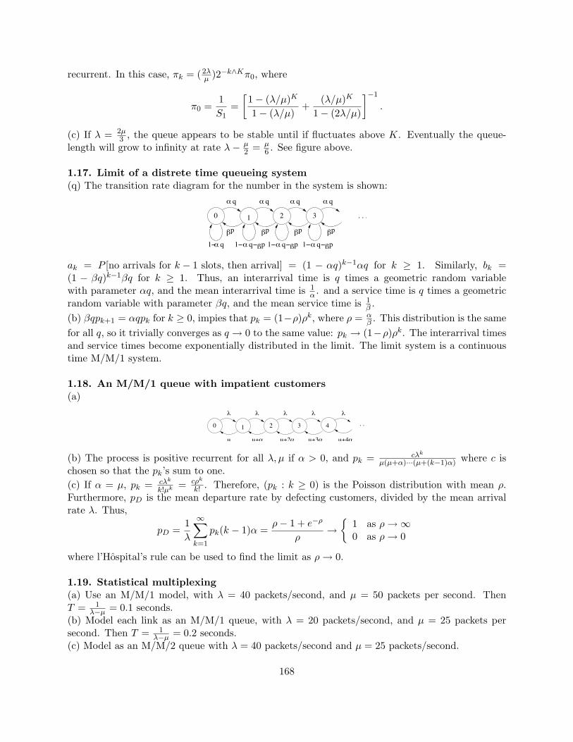
recurrent. In this case, πk = (2λµ )2−k∧Kπ0, where

π0 =1S1

=[1− (λ/µ)K

1− (λ/µ)+

(λ/µ)K

1− (2λ/µ)

]−1

.

(c) If λ = 2µ3 , the queue appears to be stable until if fluctuates above K. Eventually the queue-

length will grow to infinity at rate λ− µ2 = µ

6 . See figure above.

1.17. Limit of a distrete time queueing system(q) The transition rate diagram for the number in the system is shown:

q

q

!p

" q " q " q

!p !p !p

!" q!1! p !" q!1! p !" q!1! p

. . .31 20

1!"

"

ak = P [no arrivals for k − 1 slots, then arrival] = (1 − αq)k−1αq for k ≥ 1. Similarly, bk =(1 − βq)k−1βq for k ≥ 1. Thus, an interarrival time is q times a geometric random variablewith parameter αq, and the mean interarrival time is 1

α . and a service time is q times a geometricrandom variable with parameter βq, and the mean service time is 1

β .(b) βqpk+1 = αqpk for k ≥ 0, impies that pk = (1−ρ)ρk, where ρ = α

β . This distribution is the samefor all q, so it trivially converges as q → 0 to the same value: pk → (1−ρ)ρk. The interarrival timesand service times become exponentially distributed in the limit. The limit system is a continuoustime M/M/1 system.

1.18. An M/M/1 queue with impatient customers(a)

!

31 20 . . .4

! !

µ+" µ+2" µ+3" µ+4"

!!

µ

(b) The process is positive recurrent for all λ, µ if α > 0, and pk = cλk

µ(µ+α)···(µ+(k−1)α) where c ischosen so that the pk’s sum to one.(c) If α = µ, pk = cλk

k!µk = cρk

k! . Therefore, (pk : k ≥ 0) is the Poisson distribution with mean ρ.Furthermore, pD is the mean departure rate by defecting customers, divided by the mean arrivalrate λ. Thus,

pD =1λ

∞∑k=1

pk(k − 1)α =ρ− 1 + e−ρ

ρ→

1 as ρ →∞0 as ρ → 0

where l’Hospital’s rule can be used to find the limit as ρ → 0.

1.19. Statistical multiplexing(a) Use an M/M/1 model, with λ = 40 packets/second, and µ = 50 packets per second. ThenT = 1

λ−µ = 0.1 seconds.(b) Model each link as an M/M/1 queue, with λ = 20 packets/second, and µ = 25 packets persecond. Then T = 1

λ−µ = 0.2 seconds.(c) Model as an M/M/2 queue with λ = 40 packets/second and µ = 25 packets/second.

168

2µ

31 20 . . .4

! ! !!

µ

!

2µ 2µ 2µ

Let ρ = λ2µ . Then π0 = 0.5

0.5+ρ+ρ2+··· and πk = 2π0ρk for k ≥ 1. Thus

T =N

λ=

∑∞k=1 kρk

λ(0.5 + ρ + ρ2 + · · · )=

ρ/(1− ρ)2

λ(( 11−ρ)− 0.5)

= 0.111 seconds

We can view model (c) as a variation of (b) with statistical multiplexing at the packet level, and(a) as a variation with multiplexing at the subpacket level. Here (c) is a substantial improvementover (b), and (a) is a little better than (c).

1.20. A queue with blocking(a)

531 20 4

! ! !!

µ

!

µµµµ

πk = ρk

1+ρ+ρ2+ρ3+ρ4+ρ5 = ρk(1−ρ)1−ρ6 for 0 ≤ k ≤ 5.

(b) pB = π5 by the PASTA property.(c) W = NW /(λ(1 − pB)) where NW =

∑5k=0(k − 1)πk. Alternatively, W = N/(λ(1 − pB)) − 1

µ

(i.e. W is equal to the mean time in system minus the mean time in service)(d) π0 = 1

λ(mean cycle time for visits to state zero)= 1

λ(1/λ+mean busy period duration)There-

fore, the mean busy period duration is given by 1λ [ 1

π0− 1] = ρ−ρ6

λ(1−ρ) = ρ−ρ5

µ(1−ρ)

1.21. Multiplexing circuit and packet data streams(a) A portion of the rate diagram for C = 3 is pictured.

c

01 02 0300

10 11 12 13

20 21 22 23

30 31 32 33

ij!

!

µ

"c

(C!j)

p

j

(b) Yes, the phase structure is apparent.

(c) λp ≤ µ(C − nC) =µ

PCj=0(c−j)( λc

δC)j/j!PC

j=0( λcδC

)j/j!

1.22. Three queues and an autonomously traveling server(a) The equilibrium distribution for the server is π = (π1, π2, π3) = ( 1

αZ , 1βZ , 1

γZ ), where Z =1α + 1

β + 1γ , and the service capacity of station i is thus πi, for 1 ≤ 1 ≤ 3.

(b) The equilibrium distributions for the individual stations can be found one at a time, by themethod of phases (even though the stations are not independent). For a fixed station i, the statespace would be (l, θ) : l ≥ 0, 1 ≤ θ ≤ 3, where l is the number of customers at station i and θ is

169

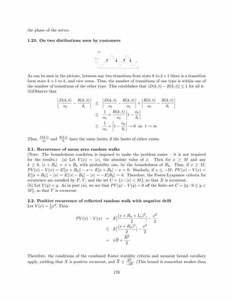
the phase of the server.

1.23. On two distibutions seen by customers

t

k

k+1

N(t)

As can be seen in the picture, between any two transtions from state k to k +1 there is a transitionform state k + 1 to k, and vice versa. Thus, the number of transitions of one type is within one ofthe number of transitions of the other type. This establishes that |D(k, t)−R(k, t)| ≤ 1 for all k.(b)Observe that ∣∣∣∣D(k, t)

αt− R(k, t)

δt

∣∣∣∣ ≤∣∣∣∣D(k, t)

αt− R(k, t)

αt

∣∣∣∣+ ∣∣∣∣R(k, t)αt

− R(k, t)δt

∣∣∣∣≤ 1

αt+

R(k, t)αt

∣∣∣∣1− αt

δt

∣∣∣∣≤ 1

αt+∣∣∣∣1− αt

δt

∣∣∣∣→ 0 as t →∞

Thus, D(k,t)αt

and R(k,t)δt

have the same limits, if the limits of either exists.

2.1. Recurrence of mean zero random walks(Note: The boundedness condition is imposed to make the problem easier – it is not requiredfor the results.) (a) Let V (x) = |x|, the absolute value of x. Then for x ≥ M and anyk ≥ 0, |x + Bk| = x + Bk with probability one, by the boundedness of Bk. Thus, if x ≥ M ,PV (x) − V (x) = E[|x + Bk|] − x = E[x + Bk] − x = 0. Similarly, if x ≤ −M , PV (x) − V (x) =E[|x + Bk|] − |x| = E[|x| − Bk] − |x| = −E[Bk] = 0. Therefore, the Foster-Lyapunov criteria forrecurrence are satisfied by P , V , and the set C = x : |x| < M, so that X is recurrent.(b) Let V (y) = y. As in part (a), we see that PV (y)− V (y) = 0 off the finite set C = y : 0 ≤ y <M, so that Y is recurrent.

2.2. Positive recurrence of reflected random walk with negative driftLet V (x) = 1

2x2. Then

PV (x)− V (x) = E[(x + Bn + Ln)2

2]− x2

2

≤ E[(x + Bn)2

2]− x2

2

= xB +B2

2

Therefore, the conditions of the combined Foster stability criteria and moment bound corollaryapply, yielding that X is positive recurrent, and X ≤ B2

−2B. (This bound is somewhat weaker than

170

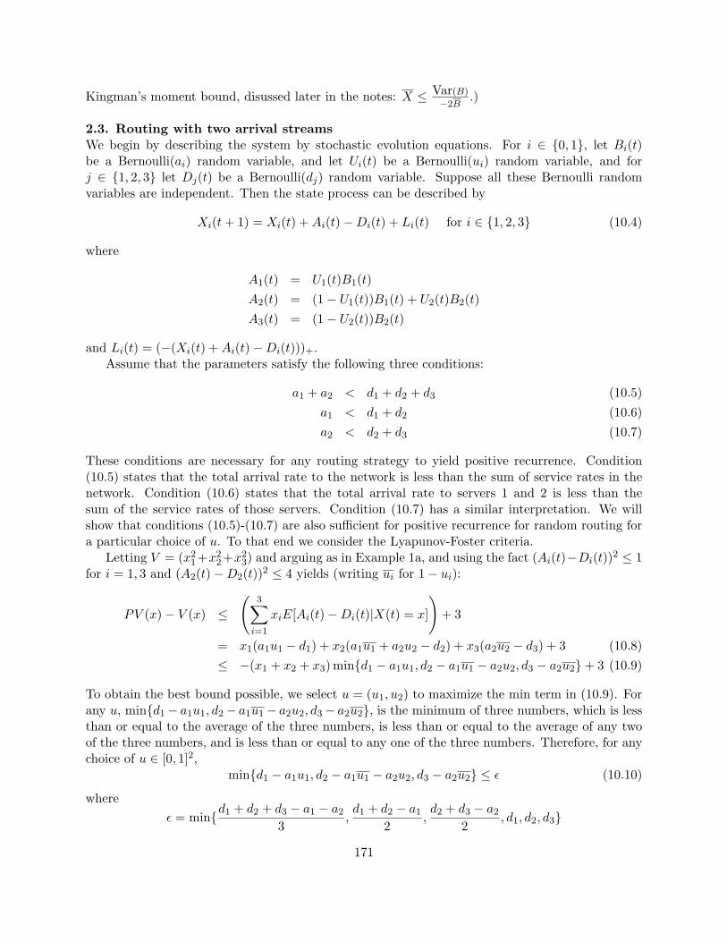
Kingman’s moment bound, disussed later in the notes: X ≤ Var(B)

−2B.)

2.3. Routing with two arrival streamsWe begin by describing the system by stochastic evolution equations. For i ∈ 0, 1, let Bi(t)be a Bernoulli(ai) random variable, and let Ui(t) be a Bernoulli(ui) random variable, and forj ∈ 1, 2, 3 let Dj(t) be a Bernoulli(dj) random variable. Suppose all these Bernoulli randomvariables are independent. Then the state process can be described by

Xi(t + 1) = Xi(t) + Ai(t)−Di(t) + Li(t) for i ∈ 1, 2, 3 (10.4)

where

A1(t) = U1(t)B1(t)A2(t) = (1− U1(t))B1(t) + U2(t)B2(t)A3(t) = (1− U2(t))B2(t)

and Li(t) = (−(Xi(t) + Ai(t)−Di(t)))+.Assume that the parameters satisfy the following three conditions:

a1 + a2 < d1 + d2 + d3 (10.5)a1 < d1 + d2 (10.6)a2 < d2 + d3 (10.7)

These conditions are necessary for any routing strategy to yield positive recurrence. Condition(10.5) states that the total arrival rate to the network is less than the sum of service rates in thenetwork. Condition (10.6) states that the total arrival rate to servers 1 and 2 is less than thesum of the service rates of those servers. Condition (10.7) has a similar interpretation. We willshow that conditions (10.5)-(10.7) are also sufficient for positive recurrence for random routing fora particular choice of u. To that end we consider the Lyapunov-Foster criteria.

Letting V = (x21+x2

2+x23) and arguing as in Example 1a, and using the fact (Ai(t)−Di(t))2 ≤ 1

for i = 1, 3 and (A2(t)−D2(t))2 ≤ 4 yields (writing ui for 1− ui):

PV (x)− V (x) ≤

(3∑

i=1

xiE[Ai(t)−Di(t)|X(t) = x]

)+ 3

= x1(a1u1 − d1) + x2(a1u1 + a2u2 − d2) + x3(a2u2 − d3) + 3 (10.8)≤ −(x1 + x2 + x3) mind1 − a1u1, d2 − a1u1 − a2u2, d3 − a2u2+ 3 (10.9)

To obtain the best bound possible, we select u = (u1, u2) to maximize the min term in (10.9). Forany u, mind1− a1u1, d2− a1u1− a2u2, d3− a2u2, is the minimum of three numbers, which is lessthan or equal to the average of the three numbers, is less than or equal to the average of any twoof the three numbers, and is less than or equal to any one of the three numbers. Therefore, for anychoice of u ∈ [0, 1]2,

mind1 − a1u1, d2 − a1u1 − a2u2, d3 − a2u2 ≤ ε (10.10)

whereε = mind1 + d2 + d3 − a1 − a2

3,d1 + d2 − a1

2,d2 + d3 − a2

2, d1, d2, d3

171

Note that ε > 0 under the necessary conditions (10.5)-(10.7). Taking u∗1 ∈ [0, 1] as large as possiblesubject to d1 − a1u

∗1 ≥ ε, and taking u∗2 ∈ [0, 1] as large as possible subject to d3 − a2u∗2 ≥ ε, yields

the choice

u∗1 =d1 − ε

a1∧ 1 u∗2 =

d3 − ε

a2∧ 1

It is not hard to check that d2 − a1u∗1 − a2u∗2 ≥ ε, so that equality holds in (10.10) for u = u∗.

This paragraph shows that the above choice of ε and u∗ can be better understood by applyingthe max-flow min-cut theorem to the flow graph shown.

v

1

q

q

q

2

3

s t

a2

d !

d !

1

3

!

!

a1d !!2

1

v

2

In addition to the source node s and sink node t, there are two columns of nodes in the graph.Nodes v1 and v2 correspond to the two arrival streams, and nodes q1, q2 and q3 correspond to thethree queues. There are three stages of links in the graph. The capacity of a link (s,vi) in thefirst stage is ai, the capacities of the links in the second graph are very large, and the capacity ofa link (qj , t) in the third stage is dj − ε. The choice of ε above is the largest possible so that (1)all links have nonnegative capacity, and (2) the capacity of any s − t cut is greater than or equalto a1 + a2. Thus, the min flow max cut theorem insures that there exists an s− t flow with valuea1 + a2. Then, u∗i can be taken to be the fraction of the flow into vi that continues to qi, for i = 1and i = 2.

Under (10.5)-(10.7) and using u∗, we have PV (x) − V (x) ≤ −ε(x1 + x2 + x3) + 3. Thus, thesystem is positive recurrent, and X1 + X2 + X3 ≤ 3

ε .1

(b) Suppose each arrival is routed to the shorter of the two queues it can go to. For simplicity, letsuch decisions be based on the queue lengths at the beginning of the slot. As far as simple boundsare concerned, there is no need, for example, to take into account the arrival in the top branch whenmaking the decision on the bottom branch, although presumably this could improve performance.Also, it might make sense to break ties in favor of queues 1 and 3 over queue 2, but that is notvery important either. We can denote this route-to-shorter policy by thinking of u in part (a) asa function of the state, u = φRS(x). Note that for given x, this choice of u minimizes the righthand side of (10.8). In particular, under the route-to-shorter policy, the right hand side of (10.8)is at least as small as its value for the fixed control u∗. Therefore, writing PRS for the one-steptransition matrix for the route to shorther policy, PRSV (x)− V (x) ≤ −ε(x1 + x2 + x + 3) + 3, andunder the necessary condtions (10.5)-(10.7), the system is positive recurrent, and X1+X2+X3 ≤ 3

ε .

2.4. An inadequacy of a linear potential functionSuppose x is on the postive x2 axis (i.e. x1 = 0 and x2 > 0). Then, given X(t) = x, duringthe slot, queue 1 will increase to 1 with probability a(1 − d1) = 0.42, and otherwise stay at zero.

1By using the fact that Xi = 0 if the arrival rate to queue i is zero, it can be shown that for u = u∗, X1+X2+X3 ≤3ε′ , where ε′ = min d1+d2+d3−a1−a2

3, d1+d2−a1

2, d2+d3−a2

2.

172

Queue 2 will decrease by one with probability 0.4, and otherwise stay the same. Thus, the driftof V , E[V (X(t + 1) − V (x)|X(t) = x] is equal to 0.02. Therefore, the drift is strictly positive forinfinitely many states, whereas the Foster-Lyapunov condition requires that the drift be negativeoff of a finite set C. So, the linear choice for V does not work for this example.

2.5. Allocation of serviceLet ε > 0. The largest we can make µ1(u) is m1 and the largest we can make µ3(u) is m2. Thus,we can select u so that

λ1 + ε ≤ µ1(u) and λ3 + ε ≤ µ3(u) (10.11)

if and only if m1 ≥ λ1 + ε and m2 ≥ λ3 + ε. If we select u so that equality holds in (10.11) then thevalue of µ2(u) is maximized subject to (10.11) , and it is given by

µ2(u) = m1 + m2 − µ1(u)− µ3(u) = m1 + m2 − λ1 + λ3 − 2ε

Therefore, in order that λ2 + ε ≤ µ2(u) hold in addition to (10.11), it is necessary and sufficientthat ε ≤ λ1+λ2+λ3−µ1−µ2

3 and m1 ≥ λ1 + ε and m2 ≥ λ2 + ε. Thus, the value of ε given in theexample is indeed the largest possible.

2.6. Opportunistic scheduling (Tassiulas and Ephremides [40])(a) The left hand side of (2.27) is the arrival rate to the set of queues in s, and the righthand sideis the probability that some queue in s is eligible for service in a given time slot. The condition isnecessary for the stability of the set of queues in s.(b) Fix ε > 0 so that for all s ∈ E with s 6= ∅,∑

i∈s

(ai + ε) ≤∑

B:B∩s 6=∅

w(B)

Consider the flow graph shown.

.

a b

q1

q2

qN

s 1

s 2

s N!

a2

a1

aN

sk

N!

2

1w(s )

w(s )

w(s )

w(s )k

+!

+!

+!

.

.

...

.

.

.

.

.

.

.

.

.

.

.

.

...

In addition to the source node a and sink node b, there are two columns of nodes in the graph. Thefirst column of nodes corresponds to the N queues, and the second column of nodes correspondsto the 2N subsets of E. There are three stages of links in the graph. The capacity of a link (a,qi)in the first stage is ai + ε, there is a link (qi, sj) in the second stage if and only if qi ∈ sj , and each

173

such link has capacity greater than the sum of the capacities of all the links in the first stage, andthe weight of a link (sk, t) in the third stage is w(sk).

We claim that the minimum of the capacities of all a − b cuts is v∗ =∑N

i=1(ai + ε). Here is aproof of the claim. The a− b cut (a : V − a) (here V is the set of nodes in the flow network)has capacity v∗, so to prove the claim, it suffices to show that any other a − b cut has capacitygreater than or equal to v∗. Fix any a − b cut (A : B). Let A = A ∩ q1, . . . , qN, or in words, Ais the set of nodes in the first column of the graph (i.e. set of queues) that are in A. If qi ∈ A andsj ∈ B such that (qi, sj) is a link in the flow graph, then the capacity of (A : B) is greater than orequal to the capacity of link (qi, sj), which is greater than v∗, so the required inequality is provedin that case. Thus, we can suppose that A contains all the nodes sj in the second column suchthat sj ∩ A 6= ∅. Therefore,

C(A : B) ≥∑

i∈q1,...,qN− eA(ai + ε) +

∑s⊂E:s∩ eA6=∅

w(s)

≥∑

i∈q1,...,qN− eA(ai + ε) +

∑i∈ eA

(ai + ε) = v∗, (10.12)

where the inequality in (10.12) follows from the choice of ε. The claim is proved.Therefore there is an a−b flow f which saturates all the links of the first stage of the flow graph.

Let u(i, s) = f(qi, s)/f(s, b) for all i, s such that f(s, b) > 0. That is, u(i, s) is the fraction of flowon link (s, b) which comes from link (qi, s). For those s such that f(s, b) = 0, define u(i, s) in somearbitrary way, respecting the requirements u(i, s) ≥ 0, u(i, s) = 0 if i 6∈ s, and

∑i∈E u(i, s) = Is 6=∅.

Then ai + ε = f(a, qi) =∑

s f(qi, s) =∑

s f(s, b)u(i, s) ≤∑

s w(s)u(i, s) = µi(u), as required.(c) Let V (x) = 1

2

∑i∈E x2

i . Let δ(t) denote the identity of the queue given a potential service attime t, with δ(t) = 0 if no queue is given potential service. Then P [δ(t) = i|S(t) = s] = u(i, s). Thedynamics of queue i are given by Xi(t+1) = Xi(t)+Ai(t)−Ri(δ(t))+Li(t), where Ri(δ) = Iδ=i.Since

∑i∈E(Ai(t)−Ri(δi(t)))2 ≤

∑i∈E(Ai(t))2 + (Ri(δi(t)))2 ≤ N +

∑i∈E Ai(t)2 we have

PV (x)− V (x) ≤

(∑i∈E

xi(ai − µi(u))

)+ K (10.13)

≤ −ε

(∑i∈E

xi

)+ K (10.14)

where K = N2 +

∑Ni=1 Ki. Thus, under the necessary stability conditions we have that under the

vector of scheduling probabilities u, the system is positive recurrent, and∑i∈E

Xi ≤K

ε(10.15)

(d) If u could be selected as a function of the state, x, then the right hand side of (10.13) wouldbe minimized by taking u(i, s) = 1 if i is the smallest index in s such that xi = maxj∈s xj . Thissuggests using the longest connected first (LCF) policy, in which the longest connected queue isserved in each time slot. If PLCF denotes the one-step transition probability matrix for the LCFpolicy, then (10.13) holds for any u, if P is replaced by PLCF . Therefore, under the necessarycondition and ε as in part (b), (10.14) also holds with P replaced by PLCF , and (10.15) holds for

174

the LCF policy.

2.7. Routing to two queues – continuous time modelSuppose λ < µ1 + µ2, which is a necessary condition for positive recurrence.(a) Under this condition, we can find u so that µ1 > λu and µ2 > λu. If each customer is indepen-dently routed to queue 1 with probability u, and if V (x) = (x2

1 + x22)/2, (2.20) becomes

2QV (x) =((x1 + 1)2 − x2

1

)λu +

((x2 + 1)2 − x2

2

)λu +

((x1 − 1)2+ − x2

1

)µ1 +

((x2 − 1)2+ − x2

2

)µ2.

Since (x1 − 1)2+ ≤ (xi − 1)2, it follows, with γ = λ + µ1 + µ2, that

QV (x) ≤ − (x1(µ1 − uλ) + x2(µ2 − uλ)) +γ

2. (10.16)

Thus, the combined stability criteria and moment bound applies, yielding that the process is positiverecurrent, and X1(µ1 − λ) + X2(µ2 − uλ) ≤ γ

2 .In analogy to Example 1a, we let

ε = max0≤u≤1

minµ1 − λu, µ2 − λu

= minµ1, µ2,µ1 + µ2 − λ

2

and the corresponding value u∗ of u is given by

u∗ =

0 if µ1 − µ2 < −λ

12 + µ1−µ2

2λ if |µ1 − µ2| ≤ λ1 if µ1 − µ2 > λ

For the system with u = u∗, X1 + X2 ≤ γ2ε . The remark at the end of Example 1a also carries

over, yielding that for splitting probability u = u∗, X1 + X2 ≤ γµ1+µ2−λ

(b) Consider now the case that when a packet arrives, it is routed to the shorter queue. To bedefinite, in case of a tie, the packet is routed to queue 1. Let QRS denote the transition rate matrixin case the route to short queue policy is used. Note that for any u, λ(x1u + x2u) ≥ λ(x1 ∧ x2).Thus, (10.16) continues to hold if Q is replaced by QRS . In particular, if λ < µ1 + µ2, then theprocess X under the route-to-shorter routing is positive recurrent, and X1 + X2 ≤ γ

2ε .

2.8. Stability of two queues with transfers(a) System is positive recurrent for some u if and only if λ1 < µ1+ν, λ2 < µ2, and λ1+λ2 < µ1+µ2.(b)

QV (x) =∑

y:y 6=x

qxy (V (y)− V (x))

=λ1

2[(x1 + 1)2 − x2

1] +λ2

2[(x2 + 1)2 − x2

2] +µ1

2[(x1 − 1)2+ − x2

1] +

µ2

2[(x2 − 1)2+ − x2

2] +uνIx1≥1

2[(x1 − 1)2 − x2

1 + (x2 + 1)2 − x22] (10.17)

(c) If the righthand side of (10.17) is changed by dropping the positive part symbols and droppingthe factor Ix1≥1, then it is not increased, so that

QV (x) ≤ x1(λ1 − µ1 − uν) + x2(λ2 + uν − µ2) + K

≤ −(x1 + x2) minµ1 + uν − λ1, µ2 − λ2 − uν+ K (10.18)

175

where K = λ1+λ2+µ1+µ2+2ν2 . To get the best bound on X1 + X2, we select u to maximize the min

term in (10.18), or u = u∗, where u∗ is the point in [0, 1] nearest to µ1+µ2−λ1−λ2

2ν . For u = u∗, wefind QV (x) ≤ −ε(x1 + x2) + K where ε = minµ1 + ν − λ1, µ2 − λ2,

µ1+µ2−λ1−λ2

2 . Which of thethree terms is smallest in the expression for ε corresponds to the three cases u∗ = 1, u∗ = 0, and0 < u∗ < 1, respectively. It is easy to check that this same ε is the largest constant such that thestability conditions (with strict inequality relaxed to less than or equal) hold with (λ1, λ2) replacedby (λ1 + ε, λ2 + ε).

2.9. Stability of a system with two queues and modulated serverBy inspection, the equilibrium distribution of the server state is (w(0), w(1), w(2)) = (1

2 , 14 , 1

4).Thus, over the long run, the server can serve queue 1 at most 3

4 of the time, it can serve queue2 at most 3

4 of the time, and, of course, it can offer at most one service in each slot. Thus, it isnecessary that a1 < 3

4 , a2 < 34 , and a1 + a2 < 1. (It can be shown that these conditions are also

sufficient for stability by using the Lyapunov function V (x) = x21+x2

22 applied to the time-sampled

process Y (n) = X(nk), where k is a constant large enough so that the mean fraction of time theserver is in each state over k time slots is close to the statistical average, no matter what the stateof the server at the beginning of such interval.)

3.1. A queue with customers arriving in pairs(a)

. . .31 20 4

µ µ µ µ µ

! ! ! ! !

(b) For any function V on Z, QV (x) = λ(Q(x+2)−Q(x))+µ(Q((x−1)+)−Q(x)). In particular, ifV (x) = x, then QV (x) = −(µ− 2λ) +µIx=0. Therefore, by the Foster-Lypunov stability criteria,if µ ≥ 2λ, then N is recurrent, and if µ > 2λ, then N is positive recurrent.(c) Take V (x) = x2

2 . Then,

QV (x) =−x(µ− 2λ) + 4λ+µ

2 if x ≥ 12λ if x = 0

Thus QV (x) ≤ −x(µ − 2λ) + 4λ+µ2 for all x ∈ Z. Conclude by the combined Foster-Lyapunov

criteria and moment bounds that if µ > 2λ, then N is positive recurrent, and N ≤ 4λ+µ2(µ−2λ) .

(d) Since the process is not explosive, it is positive recurrent if and only if there is a probabilitydistribution p so that pQ = 0. The equation pQ = 0 means that the net probability flux into eachstate should be zero. Equivalently, pQ = 0 means that the next flux out of the set 0, 1, . . . , kis zero for each k ≥ 0. Defining p−1 = 0 for convenience, the equation pQ = 0 is equivalentto the set of equations: (pk−1 + pk)λ = pk+1µ for k ≥ 0. (This is a set of second order lineardifference equations.) Multiply each side of the kth equation by zk+1, sum from k = 0 to ∞ toyield (z2λ + zλ)P (z) = µ(P (z)− po), so that

P (z) =p0

1− (λz/µ)− (λz2/µ)

The condition P (1) = 1 yields that p0 = 1 − 2λ/µ, which is valid only if 2λ/µ < 1. Under that

176

condition,

P (z) =1− 2λ/µ

1− (λz/µ)− (λz2/µ)The method of partial fraction expansion can be used to express P as the sum of two terms withdegree one denominators. First, P is rewritten as

P (z) =1− 2λ/µ

(1− z/a)(1− z/b)

where a and b are the poles of P (i.e. the zeros of the denominator), given by

a =−1 +

√1 + 4µ

λ

2b =

−1−√

1 + 4µλ

2

Matching P and its partial fraction expansion near the poles yields

P (z) = (1− 2λ/µ)[

1(1− z/a)(1− a/b)

+1

(1− b/a)(1− z/b)

]so that

pk = (1− 2λ/µ)[

a−k

1− a/b+

b−k

1− b/a

]k ≥ 0

(Using this expression we can also find an explicit expression for N , but it is more complicated thanthe bound on N found in part (c).) Thus, we have found that there exists a probability distributionp such that pQ = 0 if and only if 2λ/µ < 1.(e) rk = pk by the PASTA property. dk is proportional to pk+1µ for k ≥ 1, so that dk = pk+1

1−p0.

3.2. Token bucket regulation of a Poisson streamSuppose for simplicity that the tokens arrive at time 0, 1, 2, · · · , and let Xk denote the number oftokens present at time k− (Another approach would be to consider the number of tokens just aftertime k.) If βk = e−λλk

k! , then the one-step transition probability matrix for X = (Xk : k ≥ 0) is

P =

1− β0 β0

1− β0 − β1 β1 β0

1− β0 − β1 − β2 β2 β1 β0...

.... . .

1− β0 − · · · − βB−1 β1 β0

1− β0 − · · · − βB−1 β1 β0

(b) The throughput of packets is equal to the throughput of tokens, where is 1− πB. Therefore,Ploss for packets = λ−(1−πB)

λ . (The expression used here would be different for the other choice of Xmentioned in the solution to part (a)).(c) Let Z(t) denote the number of tokens present at time t. Then Z is a continuous time Markovprocess with the transition rate diagram shown.

. . .1 20 B!1 B

! ! ! ! !

1 1 1 1 1

177

Then,

Ploss for packets = P [no tokens present] =1

1 + 1λ + · · ·+ 1

λB

=λB

λB + λB−1 + · · ·+ 1

3.3. Extremality of constant interarrival times for G/M/1 queues(a) A∗

d(s) = exp(−s/λ). Let t1 have distribution function A. Then since exp(−sx) is convex in x,Jensens inequality can be applied to yield A∗(s) = E[exp(−st1)] ≥ exp(−sE[t1]) = A∗

d(s).(b) Let σo and σd be values of σ for the respective queues. Since A∗

d(µ(1−σo)) ≤ A∗(µ(1−σ0) = σ0

and A∗d is convex, it follows (see the figure) that σd ≤ σo. The assertions follow because the required

means are increasing functions of σ.

o

µ(1!")#

A ( )µ(1!")#A ( )

d

" 1

1

d "

3.4. Propagation of perturbations(a) See the solid lines in the figure. The departure times are indicated by where the solid diagonallines meet the axis, and occur at times 6,8,12,15, and 17. The waiting times in queue are 0, 4, 3,0, 1.

9

0 21 3 4 5 6 7 8 9 10 11 12 13 14 15 16 17

1

2

3

4

5

6

7

t

8

(b) The departure times are indicated by where the dashed diagonal lines meet the axis, and occurat times 6,9,13,15, and 17. The waiting times in queue are 0, 4, 4, 0, 1.(c) The departure times are indicated by where the dashed diagonal lines meet the axis, and occurat times 6,10, 14, 16, and 18. The waiting times in queue are 0, 4, 5, 1, 2.(d) The waiting times of all following customers in the same busy period increase by the sameamount. Busy periods can merge, and the waiting times of customers originally in a later busyperiod can also increase.

178

3.5. On priority M/GI/1 queues(a) The server works on a type 1 customer whenever one is present, and otherwise works on a type2 customer, if one is present. If the server is interrupted by a type 1 customer when it is working ona type 2 customer, the service of the type 2 customer is suspended until no more type 1 customersare in the system. Then service of the type 2 customer is resumed, with its remaining service timethe same as when the service was interrupted.

(b) Let λ = λ1 + λ2, ρi = λiXi, and ρ = ρ1 + ρ2. Then X =P

i λiXi

λ and X2 =P

i λiX2i

λ Type 1customers are not effected by type 2 customers, so the mean system time for type 1 customers isthe same as if there were no type 2 customers:

T1 = W1 + X1 =λ1X2

!

2(1− ρ1)+ X1

where ρ1 = λ1X1. To find an expression for T2, consider a type 2 customer. Recall that the meanwork in the system is given by λX2

2(1−ρ) . The PASTA property holds. Thus, T2 is the mean of thesum of the work already in the system when the customer arrives, the service time of the customeritself, and the amount of preempting work that arrives while the type 2 customer is in the system:

T2 =λX2

2(1− ρ)+ X2 + ρ1T2.

Solving for T2 yields

T2 =(

11− ρ1

)(λX2

2(1− ρ)+ X2

)3.6. Optimality of the µc ruleLet J(σ) =

∑i λiciWi(σ) =

∑i µiciρiWi(σ) denote the cost for permutatation σ.

Claim: Let σ be a permutation and let σ denote another permutation obtained from σ byswapping σi and σi+1 for some i. Then J(σ) < J(σ) if and only if µσicσi < µσi+1cσi+1 .

The claim is proved as follows. Since only customers of classes i and i + 1 are affected bythe swap, Wj(σ) = Wj(σ) for j 6∈ σi, σi+1. On the other hand, since class σi (i.e. class σi+1)customers have lower priority under σ than under σ, Wσi(σ) > Wσi(σ). Thus, δ > 0, where

δ = ρσiWσi(σ)− ρσiWσi(σ).

Similarly, Wσi+1(σ) < Wσi+1(σ), and furthermore by the conservation of flow equations,

ρσi+1Wσi+1(σ)− ρσi+1Wσi+1(σ) = −δ.

Therefore, J(σ)− J(σ) = (µσicσi − µσi+1cσi+1)δ. Since δ > 0, the claim follows immediately.By the claim, if σ does not satisfy the ordering condition µσ1cσ1 ≥ µσ2cσ2 ≥ . . . ≥ µσK cσK , then

σ is not optimal.Conversely, if σ does satisfy the ordering condition and if σ0 is an arbitrary ordering, there is

a sequence of orderings σ0, σ1, . . . , σp = σ so that J(σ0) ≥ J(σ1) ≥ · · · ≥ J(σp) = J(σ), so that σis optimal.

The µc rule is intuitively plausible because µc is the rate that instantaneous cost is reducedwhen a rate µ server works on a customer with instantaneous holding cost c.

179

3.7. A queue with persistent customers(a) The system is stable if and only if λD

b < 1. See part (b) for justification.(b) Under the PR service order, we can view the network as an ordinary M/GI/1 queue in whichthe service time variable X for a typical customer is D times a Geo(b) random variable. The systemis stable if ρ < 1, were ρ = λX = λD

b . Under this condition, the mean time in the system is given

by the Polleczek-Khinchine formula with ρ = λDb , X = D

b , and X2 = D2(2−b)b2

:

T = W + X =λX2

2(1− ρ)+ X =

(2− λD)D2(b− λD)

.

(c) The distribution of the number of customers in the system does not depend on the order ofservice (assuming no advance knowledge of how many times a given customer will return). So themean number of customers in the system does not depend on the service order. So by Little’slaw, the mean time in the system does not depend on the order of service. However, the FIFOorder at the queue would lead to a larger variance of total system time than the PR service or-der. (This is implied by the fact that if a1 < · · · < an and d1 < · · · < dn and ai < di, then∑

(di− ai)2 <∑

(dσi − ai)2 for any permutation σ other than the identity permutation. Note thatthe PR order is not FIFO for the queue, but is FIFO for the system.)

3.8. A discrete time M/GI/1 queueThe mean service time is 7/2, so the service rate is 2/7. Let ρ = 7p/2, which is the arrival rate, p,divided by the service rate. Also, ρ is the probability the server is busy in a time slot. Arrivals seethe system in equilibrium by the discrete time version of the PASTA property, which is true whennumbers of arrivals in distinct slots are independent. Given the server is busy during the slot ofan arrival, the residual service time γ of the customer in service is distributed over 0, 1, 2, 3, 4, 5.The total service time of the customer in service has distribution P [l = l] = fl

m1, for 1 ≤ l ≤ 6,

with mean E[L] = m2m1

= 12+22+32+42+52+62

6m1= 13

3 . Given L, γ is uniform on 0, 1, . . . , L − 1, so

E[γ] = E[L]−12 = 5

3 . Thus, W = 3.5N + (7p2 )(5

3), where N is the mean number of customers seenby an arrival, equal to pW . Solving for W yields W = 35p

6−21p for 0 ≤ p < 27 . An embedded Markov

process is given by the number of customers in the system just after the departure of a customer.To be specific, this number could include the new arrival, if any, occurring is the same slot that aservice is completed.

Here ia a second way to solve the problem, obtained by viewing the events at slot boundariesin a different order. Suppose that the customer in service exits if its service is complete, and if so,the customer at the head of the queue (if any) is moved into the server before a possible arrival isadded. In this view, a new customer still arrives to find the server busy with probability ρ = 7p

2 , butthe residual service time is distributed over 1, 2, 3, 4, 5, 6. The total service time of the customerin service hs the same sampled lifetime distribution as before , with mean E[L] = 13

3 , but here,given L, γ is uniformly distributed over 1, . . . , L, so E[γ] = 8

3 . Thus, by the PASTA property,W = 3.5N + (7p

2 )(83), where N is the mean number in the queue seen by an arrival. A customer

waiting W slots for service can be seen in the queue for W −1 observation times, so by Little’s law,N = (W−1)p. thus, W = 3.5(W−1)p+(7p

2 )(83), and solving for W yields W = 35p

6−21p for 0 ≤ p < 27 .

3.9. On stochastic ordering of sampled lifetimesIf fL ≺ gL, then

∫∞0 φ(x)fL(x)dx >

∫∞0 φ(x)gL(x)dx for any strictly decreasing positive function φ

180

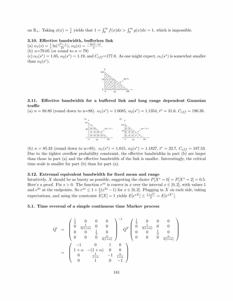
on R+. Taking φ(x) = 1x yields that 1 =

∫∞0 f(x)dx >

∫∞0 g(x)dx = 1, which is impossible.

3.10. Effective bandwidth, bufferless link(a) α1(s) = 1

s ln( e2s−12s ), α2(s) = − ln(1−s)

s .(b) n=79.05 (or round to n = 79)(c) α1(s∗) = 1.05, α2(s∗) = 1.19, and Ceff=177.0. As one might expect, α1(s∗) is somewhat smallerthan α2(s∗).

*

16879

79

148

00

A(s )

3.11. Effective bandwidth for a buffered link and long range dependent Gaussiantraffic(a) n = 88.80 (round down to n=88). α1(s∗) = 1.0085, α2(s∗) = 1.1354, t∗ = 31.6, Ceff = 190.38.

(b)

00

*A(s , t )*

18888

88

167

00

*A(s , t )*

85 184

85

154

(a)

(b) n = 85.33 (round down to n=85). α1(s∗) = 1.015, α2(s∗) = 1.1827, t∗ = 22.7, Ceff = 187.53.Due to the tighter overflow probability constraint, the effective bandwidths in part (b) are largerthan those in part (a) and the effective bandwidth of the link is smaller. Interestingly, the criticaltime scale is smaller for part (b) than for part (a).

3.12. Extremal equivalent bandwidth for fixed mean and rangeIntuitively, X should be as bursty as possible, suggesting the choice P [X∗ = 0] = P [X∗ = 2] = 0.5.Here’s a proof. Fix s > 0. The function esx is convex in x over the interval x ∈ [0, 2], with values 1and e2s at the endpoints. So esx ≤ 1 + x

2 (e2s − 1) for x ∈ [0, 2]. Plugging in X on each side, takingexpectations, and using the constraint E[X] = 1 yields E[esX ] ≤ 1+e2s

2 = E[esX∗].

5.1. Time reversal of a simple continuous time Markov process

Q′ =

13 0 0 00 1

3(1+α) 0 00 0 1

3 00 0 0 α

3(1+α)

−1

QT

13 0 0 00 1

3(1+α) 0 00 0 1

3 00 0 0 α

3(1+α)

=

−1 0 1 0

1 + α −(1 + α) 0 00 1

1+α −1 α1+α

0 1 0 −1

181

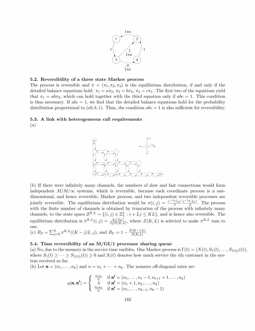
1

3

1+!

1 2

4

1

!1+!

1+!1

5.2. Reversibility of a three state Markov processThe process is reversible and π = (π1, π2, π3) is the equilibrium distribution, if and only if thedetailed balance equations hold: π1 = aπ2, π2 = bπ3, π3 = cπ1. The first two of the equations yieldthat π1 = abπ3, which can hold together with the third equation only if abc = 1. This conditionis thus necessary. If abc = 1, we find that the detailed balance equations hold for the probabilitydistribution proportional to (ab, b, 1). Thus, the condition abc = 1 is also sufficient for reversibility.

5.3. A link with heterogeneous call requirements(a)

2,0 N,0

j

i

!

! F

Si,j

0,0

0,K

0,1 1,1 2,1

1,0

(b) If there were infinitely many channels, the numbers of slow and fast connections would formindependent M/M/∞ systems, which is reversible, because each coordinate process is a one-dimensional, and hence reversible, Markov process, and two independent reversible processes arejointly reversible. The equilibrium distribution would be π(i, j) = e−λS λS

i

i!e−λF λF

j

j! . The processwith the finite number of channels is obtained by truncation of the process with infinitely manychannels, to the state space SK,L = (i, j) ∈ Z2

+ : i + Lj ≤ KL, and is hence also reversible. Theequilibrium distribution is πK,L(i, j) = λS

iλFj

i!j!Z(K,L) , where Z(K, L) is selected to make πK,L sum toone.(c) BS =

∑Lj=0 πK,L((K − j)L, j), and BF = 1− Z(K−1,L)

Z(K,L) .

5.4. Time reversibility of an M/GI/1 processor sharing queue(a) No, due to the memory in the service time varibles. One Markov process is Γ(t) = (N(t), S1(t), . . . , SN(t)(t)),where S1(t) ≥ · · · ≥ SN(t)(t)) ≥ 0 and Si(t) denotes how much service the ith customer in the sys-tem received so far.(b) Let nnn = (n1, . . . , nk) and n = n1 + · · ·+ nk. The nonzero off-diagonal rates are

q(nnn,n′n′n′) =

niµi

n if n′n′n′ = (n1, . . . , ni − 1, ni+1 + 1, . . . , nk)λ if n′n′n′ = (n1 + 1, n2, . . . , nk)

nkµkn if n′n′n′ = (n1, . . . , nk−1, nk − 1)

182

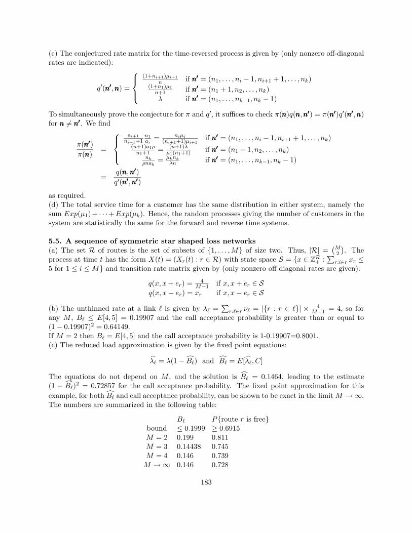
(c) The conjectured rate matrix for the time-reversed process is given by (only nonzero off-diagonalrates are indicated):

q′(n′n′n′,nnn) =

(1+ni+1)µi+1

n if n′n′n′ = (n1, . . . , ni − 1, ni+1 + 1, . . . , nk)(1+n1)µ1

n+1 if n′n′n′ = (n1 + 1, n2, . . . , nk)λ if n′n′n′ = (n1, . . . , nk−1, nk − 1)

To simultaneously prove the conjecture for π and q′, it suffices to check π(nnn)q(nnn,n′n′n′) = π(n′n′n′)q′(n′n′n′,nnn)for nnn 6= n′n′n′. We find

π(n′n′n′)π(nnn)

=

ai+1

ni+1+1n1ai

= niµi

(ni+1+1)µi+1if n′n′n′ = (n1, . . . , ni − 1, ni+1 + 1, . . . , nk)

(n+1)a1ρn1+1 = (n+1)λ

µ1(n1+1) if n′n′n′ = (n1 + 1, n2, . . . , nk)nk

ρnak= µknk

λn if n′n′n′ = (n1, . . . , nk−1, nk − 1)

=q(nnn,n′n′n′)q′(n′n′n′,n′n′n′)

as required.(d) The total service time for a customer has the same distribution in either system, namely thesum Exp(µ1)+ · · ·+Exp(µk). Hence, the random processes giving the number of customers in thesystem are statistically the same for the forward and reverse time systems.

5.5. A sequence of symmetric star shaped loss networks(a) The set R of routes is the set of subsets of 1, . . . ,M of size two. Thus, |R| =

(M2

). The

process at time t has the form X(t) = (Xr(t) : r ∈ R) with state space S = x ∈ ZR+ :∑

r:i∈r xr ≤5 for 1 ≤ i ≤ M and transition rate matrix given by (only nonzero off diagonal rates are given):

q(x, x + er) = 4M−1 if x, x + er ∈ S

q(x, x− er) = xr if x, x− er ∈ S

(b) The unthinned rate at a link ` is given by λ` =∑

r:`∈r ν` = |r : r ∈ `| × 4M−1 = 4, so for

any M , B` ≤ E[4, 5] = 0.19907 and the call acceptance probability is greater than or equal to(1− 0.19907)2 = 0.64149.If M = 2 then B` = E[4, 5] and the call acceptance probability is 1-0.19907=0.8001.(c) The reduced load approximation is given by the fixed point equations:

λ` = λ(1− B`) and B` = E[λ`, C]

The equations do not depend on M , and the solution is B` = 0.1464, leading to the estimate(1 − B`)2 = 0.72857 for the call acceptance probability. The fixed point approximation for thisexample, for both B` and call acceptance probability, can be shown to be exact in the limit M →∞.The numbers are summarized in the following table:

B` Proute r is freebound ≤ 0.1999 ≥ 0.6915M = 2 0.199 0.811M = 3 0.14438 0.745M = 4 0.146 0.739

M →∞ 0.146 0.728

183

6.1. Deterministic delay constraints for two servers in series(a) The total arrival stream to the first queue is (σ1 + σ2, ρ1 + ρ2) constrained, and the server isFIFO, so the delay is bounded above by d1 = dσ1+σ2

C1e. (d1 = 2 for the example.)

(b) Stream 1 at the output of queue 1 is (σ1 + ρ1d1, ρ1)-upper constrained, because A1 is (σ1, ρ1)-upper constrained and delay in the first queue is less than or equal to d1. (σ = σ1 + ρ1d1 = 8 forthe example.)(c) By the example after Propositoin 6.3.2, there is a bound on the delay of the lower prioritystream for a FIFO server, constant service rate C, and (σ, ρ) constrained inputs. This yields:

delay for stream 1 in queue 2 ≤ (σ1 + ρ1d1) + σ3

C2 − ρ3=

123

= 4 (for the example)

6.2. Calculation of an acceptance region based on the SCED algorithm(a) Let g(t) = σ + ρt for ρ, σ > 0. By the definition given in the notes, g∗(0) = 0 and for t ≥ 1,g∗(t) = ming(s1) + · · · + g(sn) : n ≥ 1, s1, . . . , sn ≥ 1, s1 + · · · + sn = t = minσn + ρt : n ≥1 = σ + ρt. Another approach to this problem is to use the definition of g∗ in [5]. Yet anotherapproach is to let g0(t) = It≥1g(t) and show that g0 is the maximal subadditive function equal to0 at 0, and less than or equal to g.(b) Before working out special cases, let’s work out the general case. Let g(t) = σ + ρt andf(t) = (t − d)+ where σ > 0, D > 0, r > ρ > 0. To find g∗ ? f by a graphical method, we use theformula (g∗ ? f)(t) = min0≤s≤tg∗(s) + f(t− s). That is, g∗ ? f is the minimum of the functionsobtained by considering g∗(s) + f(t− s) as a function of t on the interval t ≥ s for each s fixed.

!

" #$"%!% !"&!

!

! + " (#!")

So, for the parameters at hand,

t

4 9 20 24

20 24

25

4036

slope 1

slope 424

slope 6

slope 5t

(c) Since n1g∗1 ? f1 + n2g

∗2 ? f2 is piecewise linear with intial value 0, this function is less than or

equal to Ct for all t ≥ 0 if inequality is true at breakpoints and at +∞ (i.e. in the limit as t →∞).This requires n1(25, 36, 40, 1) + n2(0, 0, 24, 4) ≤ (900, 2000, 2400, 100), which simplifies to n1 ≤ 36and n1 + 4n2 ≤ 100.

184

100

36 60 100

25

6.3. Serve longer service priority with deterministically constrained arrival processes(a) The two queues combined is equivalent to a single queue system, with a work conservingserver that serves up to C customers per slot. The total arrival stream is (σ1 + σ2, ρ1 + ρ2)-upperconstrained, so that the maximum combined carry over for a given slot t to the next satisfiesq(t) ≤ σ1 + σ2.(b) By the same reason, the delay bound based on system busy periods can be applied to yieldd ≤ b σ1+σ2−1

C−ρ1−ρ2c.

(c) Under FIFO service within each stream and service to longer queue, each customer from stream1 exits no later than it would exit from a system with the same arrival streams, FIFO service withineach stream, and pure priority to type 2 customers, a case considered in the notes and class. Thedelay is thus bounded above by σ1+σ2

C−ρ2.

7.1. A shortest path problem(a)

2412 14 23 4

22 103 1 8 29

15 15

2

7 11 17 27 6165

13 9

s12

5

16 21 43

3762

9

14

37

2819

(b) Yes, because Dj > Di + dij for every edge ij not in the tree.(c) Synchronous Bellman-Ford would take 8 iterations (on the 9th iteration no improvement wouldbe found) because the most hops in a minimum cost path is 8.

7.2. A minumum weight spanning tree problem

s 12 14 23 4

22 103 1 8 29

15 15

2

7 11 17 27 6165

13 9

The MWST is unique because during execution of the Prim-Dijkstra algorithm there were no ties.(The sufficiency of this condition can be proved by a slight modification of the induction proof usedto prove the correctness of the Prim-Dijkstra algorithm. Suppose the Prim-Dijkstra algorithm isexecuted. Prove by induction the following claim: The set of k edges found after k steps of thealgorithm is a subset of all MWST’s.)

7.3. A maximum flow problemThe capacities, a maximum flow, and a minimum cut, are show. The maximum flow value is 15.

185

t

s

1/122/6

11/5

15/0 4/4 3/3

3/312/9 23/10 29/11

16/912/119/82/2

6/6

7/615/6

13/7 1/114/11

27/141/1

8.1. A flow deviation problem (Frank-Wolfe method)(a) Initially the 8 links directed counter clockwise along the perimeter of the network carry zeroflow, and the other 16 links carry flow b. So cost(f)=8b2.(b) Flow f uses the 8 links not used initially, as shown.

(b)

y

(a)

Thus, cost(αf + (1 − α)f) = 8(2αb)2 + 16((1 − α)b)2. Minimizing over α, we find α∗ = 13 . Under

the new flow, f1 = α∗f + (1−α∗)f , all 24 links carry flow 2b3 . The first derivative link length of all

paths used is minimum. So f1 is an optimal flow.

8.2. A simple routing problem in a queueing networkIn equilibrium, the stations are independent and have the distribution of isolated M/M/1 queues,and the delay in an M/M/1 queue with arrival rate λ and departure rate µ is 1

µ−λ . Therefore,

Da =1

2− (1 + p)and Db(p) = p

(1

2− (1 + p)

)+ (1− p)

(1

2− (1− p)+

12− (1− p)

)(b)

p=0.17

0Da

Db

0 1 21.5

1

1.5

2p=0

p=1/3

(c) p = 0 minimizes Da, because Da is increasing in p.(d) Setting D′

b(p) = 0 yields p = 13 .

(e) Setting D′a(p) + D′

b(p) = 0 yields p ≈ 0.17. Only one iteration of the flow deviation algorithmis necessary because the only degree of freedom is the split for flow b between two paths. The line

186

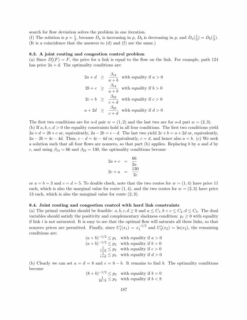
search for flow deviation solves the problem in one iteration.(f) The solution is p = 1

3 , because Da is increasing in p, Db is decreasing in p, and Da(13) = Db(1

3).(It is a coincidence that the answers to (d) and (f) are the same.)

8.3. A joint routing and congestion control problem(a) Since D′

l(F ) = F , the price for a link is equal to the flow on the link. For example, path 124has price 2a + d. The optimality conditions are:

2a + d ≥ β14

a + bwith equality if a > 0

2b + c ≥ β14

a + bwith equality if b > 0

2c + b ≥ β23

c + dwith equality if c > 0

a + 2d ≥ β23

c + dwith equality if d > 0

The first two conditions are for o-d pair w = (1, 2) and the last two are for o-d pari w = (2, 3).(b) If a, b, c, d > 0 the equality constraints hold in all four conditions. The first two conditions yield2a+ d = 2b+ c or, equivalently, 2a− 2b = c− d. The last two yield 2c+ b = a+2d or, equivalently,2a− 2b = 4c− 4d. Thus, c− d = 4c− 4d or, equivalently, c = d, and hence also a = b. (c) We seeka solution such that all four flows are nonzero, so that part (b) applies. Replacing b by a and d byc, and using β14 = 66 and β23 = 130, the optimality conditions become

2a + c =662a

2c + a =1302c

or a = b = 3 and c = d = 5. To double check, note that the two routes for w = (1, 4) have price 11each, which is also the marginal value for route (1, 4), and the two routes for w = (2, 3) have price13 each, which is also the marginal value for route (2, 3).

8.4. Joint routing and congestion control with hard link constraints(a) The primal variables should be feasible: a, b, c, d ≥ 0 and a ≤ C1, b + c ≤ C2, d ≤ C3. The dualvariables should satisfy the positivity and complementary slackness condition: pi ≥ 0 with equalityif link i is not saturated. It is easy to see that the optimal flow will saturate all three links, so thatnonzero prices are permitted. Finally, since U ′

1(x1) = x−1/21 and U ′

2(x2) = ln(x2), the remainingconditions are:

(a + b)−1/2 ≤ p1 with equality if a > 0(a + b)−1/2 ≤ p2 with equality if b > 0

1c+d ≤ p2 with equality if c > 01

c+d ≤ p3 with equality if d > 0

(b) Clearly we can set a = d = 8 and c = 8 − b. It remains to find b. The optimality conditionsbecome

(8 + b)−1/2 ≤ p2 with equality if b > 01

16−b ≤ p2 with equality if b < 8

187

Since (8 + b)−1/2 > 116−b over the entire range 0 ≤ b ≤ 8, the optimal choice of b is b = 8. This

yields the assignment (a, b, c, d) = (8, 8, 0, 8), price vector (p1, p2, p3) = (14 , 1

4 , 18), and maximum

value 2 + ln(8).

8.5. Sufficiency of the optimality condition for hard link constraintsSince L(x, p) is concave in x, for any ε with 0 < ε < 1,

L(x, p)− L(x∗, p) ≤ 1εL(x∗ + ε(x− x∗), p)− L(x∗, p)

Taking the limit as ε → 0 yields

L(x, p)− L(x∗, p) ≤∑

r

U ′r(x

∗r)(xr − x∗r) −

∑l

pl(∑r:l∈r

xr − x∗r)

=∑

r

(xr − x∗r)

U ′

r(x∗r)−

∑l∈r

pl

≤ 0 (10.19)

where the final inequality follows from the fact that for each r, the quantity in braces in (10.19) isless than or equal to zero, with equality if x∗r > 0.(b) Note that

∑l pl(Cl−

∑r:l∈r x∗r) = 0 and if Ax ≤ C, then

∑l pl(Cl−

∑r:l∈r xr) ≥ 0. So if x ≥ 0

and Ax ≤ C, ∑r

U(x∗r) = L(x∗, p) ≥ L(x, p) ≥∑

r

U(xr).

8.6. Fair flow allocation with hard constrained links(a) By inspection, xmax−min = (1

3 , 13 , 1

3 , 13).

(b) (proportional fairness) Let pl denote the price for link l. Seek a solution to the equations

x1 =1

p1 + p2 + p3x2 =

1p1 + p2

x3 =1p1

x4 =1

p2 + p3

x1 + x2 + x3 ≤ 1, with eqaulity if p1 > 0x1 + x2 + x4 ≤ 1, with eqaulity if p2 > 0

x1 + x4 ≤ 1, with eqaulity if p3 > 0

Clearly x1+x4 < 1, so that p3 = 0. Also, links 1 and 2 will be full, so that x3 = x4. But x3 = 1p1

andx4 = 1

p3, so that p1 = p2. Finally, use 1

2p1+ 1

2p1+ 1

p1to get p1 = p2 = 2, yielding xpf = (1

4 , 14 , 1

2 , 12).

Flows 1 and 2 use paths with price p1 + p2 = 4 and each have rate 14 .

Flows 3 and 4 use paths with price p1 = p2 = 2 and each have rate 12 .

9.1. Illustration of dynamic programming – a stopping time problem(a) Consider the game for a possible n + 1 observations. After seeing X1, the player can either sopand receive reward X1, or continue and receive expected reward Vn. Thus, Vn+1 = E[X1 ∨ Vn] =∫∞0 (x ∨ Vn)e−xdx =

∫ Vn

0 Vne−xdx +∫∞Vn

xe−xdx = Vn + e−Vn .(b) The optimal policy is threshold type. For 1 ≤ k ≤ n− 1, the player should stop after observingXk if Xk ≥ Vn−k. The rule for n = 8 is pictured.

188

2

4 6 7 85321

V7 V6

V1X

X

X

XStop!

1

2

3

4

1

(c)

n Vn 1 + 12 + · · ·+ 1

n

1 1.00000 1.000002 1.36788 1.500003 1.62253 1.833334 1.81993 2.083335 1.98196 2.283336 2.11976 2.450007 2.23982 2.592868 2.34630 2.717869 2.44202 2.8289710 2.52901 2.9289720 3.12883 3.5977430 3.49753 3.99499

9.2. Comparison of four ways to share two servers(a) System 1: Each of the two subsystems is an M/M/1 queue, so that N1 is twice the mean numberin an M/M/1 queue with arrival rate λ and departure rate µ: N1 = 2ρ

1−ρ .System 2: Each of the two subsystems is G/M/1 where the interarrival distribution is the same asthe sum of two exponential random variables with parameter 2λ. We will analyze such a G/M/1queue. The Laplace transform of the interarrival distribution is A∗(s) = (

∫∞0 e−st2λe−2λtdt)2 =

( 2λs+2λ)2. We seek the solution σ in the range 0 ≤ σ < 1 of the equation σ = A∗(µ − µσ), or

σ3 − 2(1 + 2ρ)σ2 + (1 + 4ρ(1 + ρ))σ − 4ρ2 = 0. Since σ = 1 is a solution, this equation can bewritten as (σ−1)(σ2− (1+4ρ)σ +4ρ2) = 0 which has solutions σ = 1 and σ = (1+4ρ)±

√1+8ρ

2 . Thus,there is a solution σ ∈ [0, 1) if and only if 0 ≤ ρ < 1, and it is given by σ = 1+4ρ−

√1+8ρ

2 . Therefore,N2 = 2ρ

1−σ = 4ρ1−4ρ+

√1+8ρ

.System 3 The third system is an M/M/2 queueing system. The number in the system is a birth-death Markov process with arrival rates λk = 2λ for all k ≥ 0 and death rates µk = (k ∧ 2)µ fork ≥ 1. Let ρ = λ

µ . The usual solution method for birth-death processes yields that p1 = 2λµ p0 and

pk = 2ρkp0 for k ≥ 1. The process is positive recurrent if and only if ρ < 1, and for such ρ we findp0 = (1 + 2(ρ + ρ2 + · · · )) = 1−ρ

1+ρ and N3 = 2ρ1−ρ2 , which is smaller than N1 by a factor 1 + ρ.

(b) For 0 < ρ < 1, N3 < N4 < N2 < N1. Here is the justification. First, we argue that N3 < N4,using the idea of stochastic domination. Indeed, let there be three independent Poisson streams: anarrival stream A with rate 2λ, and for i = 1, 2 a potential departure stream Di with departure rateµi. Consider systems 3 and 4 running, using these same three processes. If stream Di has a jumpat time t, then there is a departure from system 3 if queue i is not empty, and there is a departurefrom system 4 if the entire system is not empty. By induction on the number of events (arrival orpotential departure events) we see that the number of customers in system 3 is always less thanor equal to the number of customers in system 4, and is occasionally strictly less. Thus, N3 < N4.We argue using dynamic programming that system 4, using send to the shorter queue, is using the

189

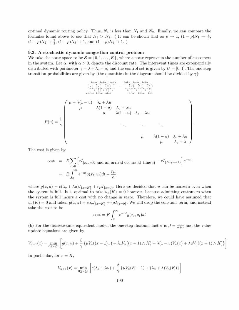
optimal dynamic routing policy. Thus, N4 is less than N1 and N2. Finally, we can compare theformulas found above to see that N1 > N2. ( It can be shown that as ρ → 1, (1 − ρ)N1 → 2

3 ,(1− ρ)N2 → 2

3 , (1− ρ)N3 → 1, and (1− ρ)N4 → 1. )

9.3. A stochastic dynamic congestion control problemWe take the state space to be S = 0, 1, . . . ,K, where a state represents the number of customersin the system. Let α, with α > 0, denote the discount rate. The interevent times are exponentiallydistributed with parameter γ = λ + λo + µ, and the control set is given by U = [0, 1]. The one steptransition probabilities are given by (the quantities in the diagram should be divided by γ):

o! (1!u)! (1!u)!µ+!(1!u)

! +!o u ! +!o u ! +!o u ! +!o u ! +!o u

(1!u)!

. . . ""#1"#20 1 2

µ µ µµµ µ

! +!o u

! +!(1!u)

P (u) =1γ

µ + λ(1− u) λo + λuµ λ(1− u) λo + λu

µ λ(1− u) λo + λu

. . . . . . . . .

µ λ(1− u) λo + λuµ λo + λ

.

The cost is given by

cost = E∑t>0

[cIxt−=K and an arrival occurs at time t − rI4xt=−1

]e−αt

= E

∫ ∞

0e−αtg(xt, ut)dt− rµ

α

where g(x, u) = c(λo + λu)Ix=K + rµIx=0. Here we decided that u can be nonzero even whenthe system is full. It is optimal to take un(K) = 0 however, because admitting customers whenthe system is full incurs a cost with no change in state. Therefore, we could have assumed thatun(K) = 0 and taken g(x, u) = cλoIx=K+ rµIx=0. We will drop the constant term, and insteadtake the cost to be

cost = E

∫ ∞

0e−αtg(xt, ut)dt

(b) For the discrete-time equivalent model, the one-step discount factor is β = αα+γ and the value

update equations are given by

Vn+1(x) = min0≤u≤1

[g(x, u) +

β

γµVn((x− 1)+) + λoVn((x + 1) ∧K) + λ(1− u)Vn(x) + λuVn((x + 1) ∧K)

]In particular, for x = K,

Vn+1(x) = min0≤u≤1

[c(λo + λu) +

β

γµVn(K − 1) + (λo + λ)Vn(K)

]190

so we see that indeed u = 0 is optimal when x = K. Thus, using g(x, u) = cλoIx=K + rµIx=0.we have that

Vn+1(x) = g(x) +β

γ[µVn((x− 1)+) + λoVn((x + 1) ∧K) + λ min Vn(x), Vn((x + 1) ∧K)]

(c) When there are n steps-to-go and the current state is x, an optimal control is given by

un(x) =

0 if Vn(x) ≤ Vn((x + 1) ∧K)1 if Vn(x) > Vn((x + 1) ∧K)

(d) Let us prove that for each n ≥ 1 there exists a threshold τn such that un(x) = Ix≤τn. It isenough to show that the following is true for each n ≥ 1:

(a) Vn is convex, i.e. Vn(1)− Vn(0) ≤ Vn(2)− Vn(1) ≤ · · · ≤ Vn(K)− Vn(K − 1)(b) − rγ

β ≤ Vn(1)− Vn(0)(c) Vn(K)− Vn(K − 1) ≤ cγ

β

To complete the proof, we prove (a)-(c) by induction on n. The details are very similar to thosefor the Mcontrolled/M/1 example in the notes, and are omitted.(e) For an exact formulation, we need to describe a state space. If FCFS service order is assumed, itis not enough to know the number of customers of each type in the system, so that the state spacewould be the set of sequences from the alphabet 1, 2 with length between 0 and K. We expectthe optimal control to have some monotonicity properties, but it would be hard to describe thecontrol because the state space is so complex. If instead, the service order were pure preemptiveresume priority to customers of one type, or processor sharing, then the state space could be takento be (n1, n2) : n1 ≥ 0, n2 ≥ 0, and n1 + n2 ≤ K. We expect the optimal control to have aswitching curve structure.

9.4. Control dependent cost(a)

Ex

∫ tn

0g(X(t), u(t))e−αtdt =

n−1∑k=0

Ex

∫ tk+1

tk

g(X(t), u(t))e−αtdt

=n−1∑k=0

Ex

∫ tk+1

tk

g(X(tk), wk)e−αtdt

=n−1∑k=0

Ex[g(X(tk), wk)∫ tk+1

tk

e−αtdt]

=n−1∑k=0

Ex[g(X(tk), wk)]Ex[∫ tk+1

tk

e−αtdt]

=1− β

αEx

n−1∑k=0

βkg(X(tk), wk)

where we used the fact that

Ex[∫ tk+1

tk

e−αtdt] = Ex[1α

(e−αtk − e−αtk+1)] =1α

[βk − βk+1] =(1− β)βk

α.

191

(b) The only change is that g should be added to the cost before the minimization over u, yielding:

Vn+1(x) = infu∈U

[g(x, u) + β

∑y

pxy(u)Vn(y)

].

9.5. Optimal control of a server(a) We use S = Z2

+, where state x = (x1, x2) denotes xi customers in station i, for i = 1, 2. LetA1(x1, x2) = (x1 + 1, x2) and D1(x1, x2) = ((x1 − 1)+, x2), and define A2 and D2 similarly. Then

px,y(u) =1γ

2∑i=1

(λiIy=Ai(x) + mi(u)Iy=Di(x)

)The CDF F corresponds to the exponential distribution with parameter γ = λ1 +λ2 +µ0 +µ1 +µ2,and the instantaneous cost function is g(x) = x1 + x2.(b) The backwards equation of dynamic programming becomes

Vn+1(x) = g(x) + min0≤u≤1

β

γ

2∑i=1

(λiVn(Ai(x)) + mi(u)Vn(Di(x)))

or, after plugging in the optimal value for u,

Vn+1(x) = g(x) +β

γ

[2∑

i=1

(λiVn(Ai(x)) + µi(u)Vn(Di(x))) + µ0 minVn(D1(x)), Vn(D2(x))

]

with the intial condition V0 ≡ 0.(c)

u∗n(x) =

1 if Vn(D1x) ≤ V2(D2x)0 else.

(10.20)

(d) We conjecture that the service rate µ0 should be allocated to the station with the longer queue.That is, u∗n(x) = Ix1≥x2. Equivalently, V (x1, x2) ≤ V (x1 − 1, x2 + 1) whenever 0 ≤ x1 ≤ x2 andV (x1, x2) ≤ V (x1 + 1, x2 − 1) whenever 0 ≤ x2 ≤ x1.

9.6. A dynamic server rate control problem with switching costs(a) We use the state space S = (l, θ) : l ∈ Z+, θ ∈ H,L, where for a given state x = (l, θ),l denotes the number of customers in the system and θ denotes the state of the server. Letγ = λ + µH , which is the maximum event rate that we shall use. (Another natural choice wouldbe γ = λ + µL + µH , and then the self loop transition probabilities would be increased in the onestep transition probabilities.) We take the control values u = (ua, ud) to be in the set U = [0, 1]2,where ua is the probability the server is in the high state after the next event, given the next eventis an arrival, and ud is the probability the server is in the high state after the next event, given thenext event is a departure. The following diagram gives the transition probabilities (the quantitiesshown should be divided by γ).2

2Variations of these equations are possible, depending on the exact assumptions. We chose to allow a server statechange at potential departure times, even if the potential departures are not used.

192

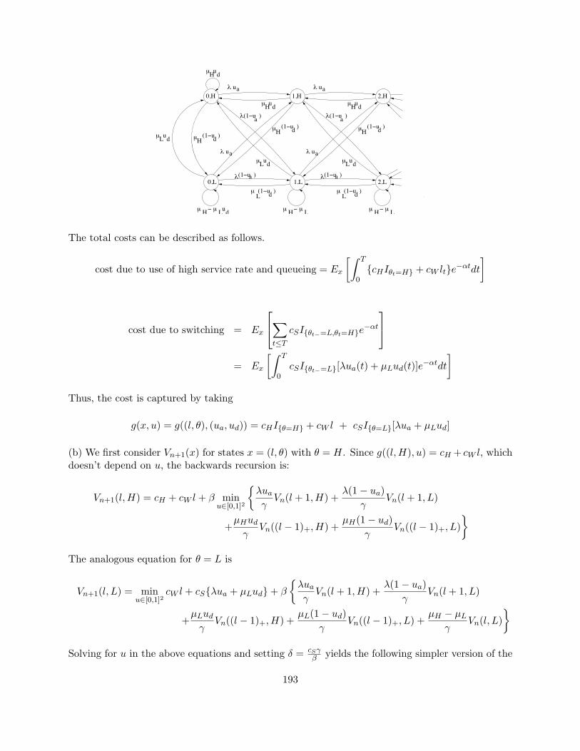
d H µ L!

µLud

(1!u )! a

(1!u )dµL

a(1!u )!

µH(1!u )d

µHud

! ua

µ H µ L!

µLud

(1!u )! a

(1!u )dµL

a(1!u )!

µHud

! ua

µHud

µ H µ L!

µLud µH(1!u )d

! ua! ua

µH(1!u )d

0,H 1,H 2,H

0,L 1,L 2,L

u µ

The total costs can be described as follows.

cost due to use of high service rate and queueing = Ex

[∫ T

0cHIθt=H + cW lte−αtdt

]

cost due to switching = Ex

∑t≤T

cSIθt−=L,θt=He−αt

= Ex

[∫ T

0cSIθt−=L[λua(t) + µLud(t)]e−αtdt

]Thus, the cost is captured by taking

g(x, u) = g((l, θ), (ua, ud)) = cHIθ=H + cW l + cSIθ=L[λua + µLud]

(b) We first consider Vn+1(x) for states x = (l, θ) with θ = H. Since g((l, H), u) = cH + cW l, whichdoesn’t depend on u, the backwards recursion is:

Vn+1(l,H) = cH + cW l + β minu∈[0,1]2

λua

γVn(l + 1,H) +

λ(1− ua)γ

Vn(l + 1, L)

+µHud

γVn((l − 1)+,H) +

µH(1− ud)γ

Vn((l − 1)+, L)

The analogous equation for θ = L is

Vn+1(l, L) = minu∈[0,1]2

cW l + cSλua + µLud+ β

λua

γVn(l + 1,H) +

λ(1− ua)γ

Vn(l + 1, L)

+µLud

γVn((l − 1)+,H) +

µL(1− ud)γ

Vn((l − 1)+, L) +µH − µL

γVn(l, L)

Solving for u in the above equations and setting δ = cSγ

β yields the following simpler version of the

193

dynamic programming backwards recursion:

Vn+1(l,H) = cH + cW l +βλ

γminVn(l + 1,H), Vn(l + 1, L) (10.21)

+βµH

γminVn((l − 1)+,H), Vn((l − 1)+, L)

Vn+1(l, L) = cW l +βλ

γminδ + Vn(l + 1,H), Vn(l + 1, L) (10.22)

+βµL

γminδ + Vn((l − 1)+,H), Vn((l − 1)+, L)+

β(µH − µL)γ

Vn(l, L)

The optimal controls can be succinctly described as follows. If the current switch state is θ, andif there will be l′ customers in the system after the next arrival or potential departure, then theoptimal server state after such arrival or potential departure is given by:

If θ = H then: Vn(l′, L) > Vn(l′,H) ⇔ new server state HIf θ = L then: Vn(l′, L) > Vn(l′,H) + δ ⇔ new server state H

(10.23)

The function Vn(l, θ) represents the cost-to-go for initial state (l, θ), with the understandingthat it is not possible to switch the server state until the first event time. Let Wn(l, θ) denote thecost-to-go, given the initial state is (l, θ), but assuming that the server state can be changed attime zero. Then the dynamic programming equations become:3

Wn(l, θ) = minVn(l, L), Vn(l, H) + δIθ=L (10.24)

Vn+1(l, θ) = cHIθ=H + cW l +βλ

γWn(l + 1, θ) +

βµL

γWn((l − 1)+, θ)

+β(µH − µL)

γ

Iθ=HWn(l − 1,H) + Iθ=LWn(l, L)

(10.25)

with the initial conditions V0 ≡ 0 and Wn ≡ 0.In the special case that there is no switching cost, δ = 0. In that case, Wn(l, θ) does not depend

on θ, so we write it as Wn(l). Then the dynamic programming equations become:

Wn(l) = minVn(l, L), Vn(l, H) (10.26)

Vn+1(l, θ) = cHIθ=H + cW l +βλ

γWn(l + 1) +

βµL

γWn((l − 1)+)

+β(µH − µL)

γ

Iθ=HWn(l − 1) + Iθ=LWn(l)

(10.27)

In the case of no switching costs, it is rather simple to show by induction on n that Wn is a convex,nondecreasing function on Z+ and Vn satisfies properties 1-5 in the original solutions. As noted inthe original solutions, property 3 for Vn implies the conjectured threshold structure.

(c) We conjecture that the optimal control has a threshold behavior, because when there aremore customers in the system, it is more valuable to quickly serve the customer in the server,thereby reducing the waiting times of all remaining customers. Since there is a switching cost,

3In this version, we allow a change of server state after any event. Thus, the functions Vn are slightly differentthan the ones above.

194

however, it is better to be a bit reluctant to switch, because excessive switching is costly. Thissuggests that the threshold for switching from H to L should be smaller than the threshold forswitching from L to H. Specifically, we expect there are two thresholds, τH and τL, with τH ≤ τL,so that the optimal control law (10.23) becomes

l′ > τθ ⇔ new server state H (10.28)

This leads to the nonzero transition probabilities shown. The transient states are included in thefirst diagram and are omitted in the second.

H . . .

. . .

!H

!L

. . .

L

H

L

We haven’t found a proof of the conjectured threshold structure in general, but we here sketch aproof in the case of zero switching cost (δ = 0). Consider the following properties of a function Von Z+ × L,H:

1. V (l, θ) is nondecreasing in l for θ = L and for θ = H.2. V (l, θ) is convex in l for θ = L and for θ = H.3. V (l + 1, L)− V (l + 1,H)− V (l, L) + V (l, H) ≥ 0 for l ≥ 0.4. V (l + 2,H)− V (l + 1,H)− V (l + 1, L) + V (l, L) ≥ 0 for l ≥ 0.5. V (l + 2, L)− V (l + 1, L)− V (l + 1,H) + V (l,H) ≥ 0 for l ≥ 0.

We write property 1.H to denote property 1 for θ = 1. Properties 1.L, 2.H, and 2.L are definedanalogously. The following figure gives a graphical representation of the five properties.

+!+ 2! + !

+ !+! +

!!!

2!

1.L 1.H 2.L 2.H 3 4 5HL

Property:

!+++

+++

For each property, the figure indicates the type of linear combinations of values of V which shouldbe nonnegative. The collection of properties 1-5 are nearly symmetric in H and L. Property 5 isobtained by swapping L and H in property 4. Thus, property 3 is the only part of properties 1-5that is not symmetric in L and H.

Properties 3 and 4 imply property 2 (both 2.L and 2.H). This can be seen graphically by slidingthe diagram for property 4 to the left to overlap the diagram for property 3, and adding. Similarly,properties 2.L and 3 imply property 5. Thus, properties 3 and 4 together imply properties 2 and5. So to prove a function has properties 1-5, it suffices to prove it has properties 1, 3, and 4.

Property 3 is the one connected to the threshold structure. Another way to state property 3is that V (l, H) − V (l.L) is nonincreasing in l. That is, as l increases, given there are l customersin the system, it becomes increasingly preferable to be in state H. More specifically, if Vn satisfiesproperty 3, and if τL = maxl : V (l, H)−V (l, L) ≥ 0 and τH = maxl : V (l, H)+δ−V (l, L) ≥ 0,then (10.23) is equivalent to (10.28).

It remains to show that Vn has properties 1-5 for all n ≥ 0. To do so, it can be proved byinduction on n that Vn has properties 1-5 for all n ≥ 0, and Wn is convex and nondecreasingon Z+. For the base case, observe that the function V0 given by V0 ≡ 0 has properties 1-5.

195

For the general induction step, it can be easily shown that if Vn has properties 1-5, then Wn isconvex, nondecreasing. And given that Wn is convex, nondecreasing, it can be shown that Vn+1

has properties 1-5. As mentioned above, it suffices to establish that Vn+1 has properties 1,3, and4. Unfortunately, this approach doesn’t seem to work in case δ > 0.

(d) First, if cS = 0 then the cost-to-go does not depend on the server state, and in particularthe thresholds should be equal: τL = τH . Suppose a single customer is served, with no othercustomers waiting or arriving. If the server is put into the high state, and if tH denotes the time thecustomer departs, then the average cost is E[

∫∞0 e−αtdt](cH +cW ) = E[1−e−αtH

α ](cH +cW ) = cH+cWα+µH

.Similarly, if the server is put into the low state during the service interval, then the cost is cW

α+µL.

The given inequality implies that it costs less to use the high rate, even if there is only one customerin the system over all time. But using the high rate for a given server helps decrease the costs forany other customers that might be in the system, so that it is optimal to always use the high rate(when the system is not emput), under the conditions given in the problem.

196

Bibliography

[1] S. Asmussen, Applied Probability and Queues, Wiley, New York, 1987.

[2] D. Bertsekas and R.G. Gallager, Data Networks, 2nd ed., Prentice-Hall, Englewood Cliffs,NewJersey, 1992.

[3] D.D. Botvich and N. Duffield, “Large deviations, the shape of the loss curve, and economies ofscale in large multiplexers,” Queueing Systems, vol. 20, 293-320, 1995.

[4] C.-S. Chang,“Stability, queue length, and delay of deterministic and stochastic queueing net-works,”IEEE Trans. on Automatic Control, vol. 39, no. 5, pp. 913-931, May 1994.

[5] C.-S. Chang, Performance Guarantees in Communication Networks, Springer, New York, 2001.

[6] J. Cohen and F. Kelly, “A paradox of congestion control in queueing networks,” Journal ofApplied Probability, vol. 27, 1990.

[7] C. Courcoubetis and R. Weber, “Buffer overflow asymptotics for a switch handling many trafficsources,” J. Applied Probability, vol. 33, no. 3, 886-903, 1996.

[8] R.L. Cruz, “A calculus for network delay, part I: network elements in isolation,” IEEE Trans-actions on Information Theory, vol. 37, pp. 114–131, Jan. 1991.

[9] R.L. Cruz, “A calculus for network delay, part II: network analysis,” IEEE Transactions onInformation Theory, vol. 37, pp. 132–141, Jan. 1991.

[10] R.L. Cruz, “Service burstiness and dynamic burstiness measures: a framework,” Journal ofHigh Speed Networks, vol. 1, no. 2, pp. 105-127, 1992.

[11] G. de Veciana, G. Kesidis, and J. Walrand, “Resource management in wide-area ATM networksusing effective bandwidths”, IEEE J. Selected Areas of Communications, vol. 13, no. 6, 1081-1090, 1995.

[12] J. Edmonds, “Submodular functions, matroids and certain polyhedra, Proc. Calgary Int. Conf.Combinatorial Structures and Applications, Calgary, Alta, June 1969, pp. 6987.

[13] A. Elwalid, D. Mitra, and R.H. Wentworth, “A new approach for allocating buffers and band-width to heterogeneous regulated traffic in an ATM node,” IEEE J. Selected Areas of Commu-nications, vol. 13, no. 6, pp. 991-1003, 1995.

[14] F. G. Foster, “On the stochastic matrices associated with certain queueing processes,” Ann.Math Statist., Vol. 24, pp. 355-360, 1953.

197

[15] L. Fratta, M. Gerla, and L. Kleinrock, “The flow deviation method: an approach to store andforward communication network design.” Networks, vol. 3, pp. 97-133, 1973.

[16] R.G. Gallager, P.A. Humblet, and P.M. Spira, “A distributed algorithm for minimum-weightspanning trees,” ACM Trans. Programming Languages and Systems, 1983.

[17] G.L. Georgiadis, R. Guerin, V. Peris, and K.N. Sivrajan, “Efficient network QOS provisioningbased on per node traffic shaping,” IEEE/ACM Transactions on Networking, vol. 4, no. 4, pp.482-501, August 1996.

[18] G.R. Grimmett and D.R. Stirzaker, Probability and Random Processes, 3rd Ed., Oxford Uni-versity Press, Oxford and New York, 2001.

[19] B. Hajek, ”Optimal control of two interacting service stations,” IEEE Trans. Automatic Con-trol, Vol. 29,June 1984, pp. 491-499.

[20] J.Y. Hui, “Resource allocation for broadband networks,” IEEE J. Selected Areas of Commu-nications, vol. 13, no. 6, 1598-1608.

[21] J.Y. Hui Switching an traffic theory for integrated broadband networks, Kluwer, Boston, 1990.

[22] J.Y. Hui and E. Karasan, “A thermodynamic theory of broadband networks with applicationto dynamic routing,” IEEE J. Selected Areas of Communications, vol. 13, no. 6, 991-1003, 1995.

[23] F.P. Kelly, “Notes on effective bandwidth” In Stochastic Networks Theory and Applications,F.P. Kelly, S. Zachary and I. Ziedins, Eds., Oxford Science, pp. 141-168, 1996.

[24] F. P. Kelly, “Charging and rate control for elastic traffic,” European Transactions on Telecom-munications, Vol. 8, (1997), pp. 33-37.

[25] F. P. Kelly, A.K. Maulloo, and D.K.H. Tan, “Rate control in communication networks: shadowprices, proportional fairness and stability,” Journal of the Operational Research Society 49(1998), 237-252.

[26] J.F.C. Kingman, “Some inequalitiies for the queue GI/G/1,” Biometrika, vol. 49, no. 3 and 4,p. 315-324, 1962.

[27] L. Kleinrock,, Queueing Systems, Vol, 2: Computer Applications, Wiley, 1976.

[28] P.R. Kumar and S.P. Meyn, “Stability of queueing networks and scheduling policies,” IEEETrans. Automatic Control, vol. 40, 1995, pp. 251-260.

[29] N. McKeown, A. Mekkittikul, V. Ananthraram, and J. Walrand, “Achieving 100% throuhputin an input-queued switch,” IEEE Transactions on Communications, vol. 47, no. 8, 1999.

[30] S.P. Meyn and R.L. Tweedie, Markov chains and stochastic stability, Springer-Verlag, London,1993.

[31] J. Mo and J. Walrand, “Fair end-to-end window-based congestion control,” IEEE/ACM Trans.Networking, vol. 8, pp. 556-567, 2000.

[32] J.R. Norris, Markov Chains, Cambridge University Press, Cambridge, 1997.

198

[33] A.K. Parekh, and R.G. Gallager, “A generalized processor sharing approach to flow control inintegrated services networks: the single node case,” IEEE/ACM Trans. on Networking, vol. 1,no. 3, pp. 344-357, 1993.

[34] Parekh, A.K. and R.G. Gallager, “A generalized processor sharing approach to flow controlin integrated services networks: the multiple-node case,” IEEE INFOCOM 93, San Francisco,521-530, March 1993.

[35] B.K. Ryu and A. Elwalid, “The importance of long-range dependence of VBR traffic engineer-ing: myths and realities,” Proc. ACM SIGCOMM, 3-14, August 1996.

[36] Shwartz, A., and Weiss, A. Large deviations for performance analysis, queues, communicationand computing, Chapman & Hall, London, 1995.

[37] A. Simonian and J. Guibert, “Large deviations approximations for fluid queues fed by a largenumber of sources,” IEEE J. Selected Areas of Communications, vol. 13, no. 6, 1081-1090.

[38] R. Srikant, The Mathematics of Internet Congestion Control, Birkhauser, Boston, 2003.

[39] L. Tassiulas and A. Ephremides, “Stability properties of constrained queueing systems andscheduling for maximum throughput in multihop radio networks,” IEEE Trans. AutomaticControl, vol. 37, no. 12, December 1992.

[40] L. Tassiulas and A. Ephremides, “Dynamic server allocation to parallel queues with randomlyvarying connectivity,” IEEE Trans. Information Theory, vol. 39, March 1993.

[41] L. Tassiulas, “Scheduling and performance limits of networks with constantly changing topol-ogy,” IEEE Trans. on Info. Theory, Vol. 43, No. 3, pp. 1067-1073, May 1997.

[42] R. L. Tweedie, The existence of moments of stationary Markov chains, J. Appl. Prob., vol. 20,pp. 191 - 196, 1983.

[43] W. Willinger, M.S. Taqqu, and A. Erramilli, “A bibliographical guide to self-similar trafficand performance modeling for modern high-speed networks.” In Stochastic Networks Theoryand Applications, F.P. Kelly, S. Zachary and I. Ziedins, Eds., Oxford Science, pp. 339-366,1996.

199

notes for ece 467 communication network analysis - university of

Documents