notes on introductory point-set topology

Notes on Introductory Point-Set Topology

Allen Hatcher

Chapter 1. Basic Point-Set Topology . . . . . . . . . . . . . . . 1

Topological Spaces 1, Interior, Closure, and Boundary 5, Basis for a Topology 7,

Metric Spaces 9, Subspaces 10, Continuity and Homeomorphisms 12, Product

Spaces 13, Exercises 16

Chapter 2. Connectedness . . . . . . . . . . . . . . . . . . . . 18

Path-connected Spaces 19, Cut Points 20, Connected Components and Path Com-

ponents 21, The Cantor Set 25, Exercises 28

Chapter 3. Compactness . . . . . . . . . . . . . . . . . . . . . 30

Compact Sets in Euclidean Space 31, Hausdorff Spaces 34, Normal Spaces 36,

Lebesgue Numbers 38, Infinite Products 30, Exercises 41

Chapter 4. Quotient Spaces . . . . . . . . . . . . . . . . . . . 44

Exercises 52

Basic Point-Set Topology 1

Chapter 1. Basic Point-Set Topology

One way to describe the subject of Topology is to say that it is qualitative geom-

etry. The idea is that if one geometric object can be continuously transformed into

another, then the two objects are to be viewed as being topologically the same. For

example, a circle and a square are topologically equivalent. Physically, a rubber band

can be stretched into the form of either a circle or a square, as well as many other

shapes which are also viewed as being topologically equivalent. On the other hand, a

figure eight curve formed by two circles touching at a point is to be regarded as topo-

logically distinct from a circle or square. A qualitative property that distinguishes the

circle from the figure eight is the number of connected pieces that remain when a

single point is removed: When a point is removed from a circle what remains is still

connected, a single arc, whereas for a figure eight if one removes the point of contact

of its two circles, what remains is two separate arcs, two separate pieces.

The term used to describe two geometric objects that are topologically equivalent

is homeomorphic . Thus a circle and a square are homeomorphic. Concretely, if we

place a circle C inside a square S with the same center

point, then projecting the circle radially outward to the

square defines a function f :C→S , and this function is

continuous: small changes in x produce small changes in

f(x) . The function f has an inverse f−1 :S→C obtained

by projecting the square radially inward to the circle, and

this is continuous as well. One says that f is a homeo-

morphism between C and S .

One of the basic problems of Topology is to determine when two given geometric

objects are homeomorphic. This can be quite difficult in general.

Our first goal will be to define exactly what the ‘geometric objects’ are that one

studies in Topology. These are called topological spaces. The definition turns out to

be extremely general, so that many objects that are topological spaces are not very

geometric at all, in fact.

Topological Spaces

Rather than jump directly into the definition of a topological space we will first

spend a little time motivating the definition by discussing the notion of continuity of a

function. One could say that topological spaces are the objects for which continuous

2 Chapter 1

functions can be defined.

For the sake of simplicity and concreteness let us talk about functions f :R→R .

There are two definitions of continuity for such a function that the reader may already

be familiar with, the ε -δ definition and the definition in terms of limits. But it is a

third definition, equivalent to these two, that is the one we want here. This definition

is expressed in terms of the notion of an open set in R , generalizing the familiar idea

of an open interval (a, b) .

Definition. A subset O of R is open if for each point x ∈ O there exists an interval

(a, b) that contains x and is contained in O .

With this definition an open interval certainly qualifies as an open set. Other

examples are:

R itself is an open set, as are semi-infinite intervals (a,∞) and (−∞, a) .

The complement of a finite set in R is open.

If A is the union of the infinite sequence xn = 1/n , n = 1,2, ··· , together with

its limit 0 then R−A is open.

Any union of open intervals is an open set. The preceding examples are special

cases of this. The converse statement is also true: every open set O is a union

of open intervals since for each x ∈ O there is an open interval (ax, bx) with

x ∈ (ax, bx) ⊂ O , and O is the union of all these intervals (ax, bx) .

The empty set ∅ is open, since the condition for openness is satisfied vacuously

as there are no points x where the condition could fail to hold.

Here are some examples of sets which are not open:

A closed interval [a, b] is not an open set since there is no open interval about

either a or b that is contained in [a, b] . Similarly, half-open intervals [a, b) and

(a, b] are not open sets when a < b .

A nonempty finite set is not open.

Now for the nice definition of a continuous function in terms of open sets:

Definition. A function f :R→R is continuous if for each open set O in R the inverse

image f−1(O) ={

x ∈ R∣

∣ f(x) ∈ O}

is also an open set.

To see that this corresponds to the intuitive notion of continuity, consider what

would happen if this condition failed to hold for a function f . There would then be

an open set O for which f−1(O) was not open. This means there would be a point

x0 ∈ f−1(O) for which there was no interval (a, b) containing x0 and contained in

f−1(O) . This is equivalent to saying there would be points x arbitrarily close to x0

that are in the complement of f−1(O) . For x to be in the complement of f−1(O)


means that f(x) is not in O . On the other hand, x0 was in f−1(O) so f(x0) is in

O . Since O was assumed to be open, there is an interval (c, d) about f(x0) that is

contained in O . The points f(x) that are not in O are therefore not in (c, d) so they

remain at least a fixed positive distance from f(x0) . To summarize: there are points

x arbitrarily close to x0 for which f(x) remains at least a fixed positive distance

away from f(x0) . This certainly says that f is discontinuous at x0 .

This reasoning can be reversed. A reasonable interpretation of discontinuity of

f at x0 would be that there are points x arbitrarily close to x0 for which f(x) stays

at least a fixed positive distance away from f(x0) . Call this fixed positive distance ε .

Let O be the open set (f (x0) − ε, f (x0) + ε) . Then f−1(O) contains x0 but it does

not contain any points x for which f(x) is not in O , and we are assuming there are

such points x arbitrarily close to x0 , so f−1(O) is not open since it does not contain

all points in some interval (a, b) about x0 .

The definition we have given for continuity of functions R→R can be applied

more generally to functions Rn→Rn and even R

m→Rn once one has a notion of

what open sets in Rn are. The natural definition generalizing the case n = 1 is to say

that a set O in Rn is open if for each x ∈ O there exists an open ball containing x

and contained in O , where an open ball of radius r and center x0 is defined to be

the set of points x of distance less than r from x0 . Here the distance from x to x0

is measured as in linear algebra, as the length of the vector x−x0 , the square root of

the dot product of this vector with itself.

This definition of open sets in Rn does not depend as heavily on the notion of

distance in Rn as might appear. For example in R

2 where open balls become open

disks, we could use open squares instead of open disks since if a point x ∈ O is

contained in an open disk contained in O then it is also contained in an open square

contained in the disk and hence in O , and conversely, if x is contained in an open

square contained in O then it is contained in an open disk contained in the open

square and hence in O . In a similar way we could use many other shapes besides

disks and squares, such as ellipses or polygons with any number of sides.

After these preliminary remarks we now give the definition of a topological space.

Definition. A topological space is a set X together with a collection O of subsets of

X , called open sets, such that:

(1) The union of any collection of sets in O is in O .

(2) The intersection of any finite collection of sets in O is in O .

(3) Both ∅ and X are in O .

4 Chapter 1

The collection O of open sets is called a topology on X .

All three of these conditions hold for open sets in R as defined earlier. To check

that (1) holds, suppose that we have a collection of open sets Oα where the index

α ranges over some index set I , either finite or infinite. A point x ∈⋃

αOα lies in

some Oα , which is open so there is an interval (a, b) with x ∈ (a, b) ⊂ Oα , hence

x ∈ (a, b) ⊂⋃

αOα so⋃

αOα is open. To check (2) it suffices by induction to check

that the intersection of two open sets O1 and O2 is open. If x ∈ O1∩O2 then x lies

in open intervals in O1 and O2 , and there is a smaller open interval in the intersection

of these two open intervals that contains x . This open interval lies in O1 ∩ O2 , so

O1 ∩O2 is open. Finally, condition (3) obviously holds for open sets in R .

In a similar fashion one can check that open sets in R2 or more generally Rn also

satisfy (1)–(3).

Notice that the intersection of an infinite collection of open sets in R need not

be open. For example, the intersection of all the open intervals (−1/n,1/n) for n =

1,2, ··· is the single point {0} which is not open. This explains why condition (2) is

only for finite intersections.

It is always possible to construct at least two topologies on every set X by choos-

ing the collection O of open sets to be as large as possible or as small as possible:

The collection O of all subsets of X defines a topology on X called the discrete

topology.

If we let O consist of just X itself and ∅ , this defines a topology, the trivial

topology.

Thus we have three different topologies on R , the usual topology, the discrete topol-

ogy, and the trivial topology. Here are two more, the first with fewer open sets than

the usual topology, the second with more open sets:

Let O consist of the empty set together with all subsets of R whose complement

is finite. The axioms (1)–(3) are easily verified, and we leave this for the reader to

check. Every set in O is open in the usual topology, but not vice versa.

Let O consist of all sets O such that for each x ∈ O there is an interval [a, b) with

x ∈ [a, b) ⊂ O . Properties (1)–(3) can be checked by almost the same argument

as for the usual topology on R , and again we leave this for the reader to do.

Intervals [a, b) are certainly in O so this topology is different from the usual

topology on R . Every interval (a, b) is in O since it can be expressed as a union

of an increasing sequence of intervals [an, b) in O . It follows that O contains all


sets that are open in the usual topology since these can be expressed as unions

of intervals (a, b) .

These examples illustrate how one can have two topologies O and O′

on a set X ,

with every set that is open in the O topology is also open in the O′

topology, so

O ⊂ O′ . In this situation we say that the topology O

′ is finer than O and that O is

coarser than O′. Thus the discrete topology on X is finer than any other topology

and the trivial topology is coarser than any other topology. In the case X = R we

have interpolated three other topologies between these two extremes, with the finite-

complement topology being coarser than the usual topology and the half-open-interval

topology being finer than the usual topology. Of course, given two topologies on a set

X , it need not be true that either one is finer or coarser than the other.

Here is another piece of basic terminology:

Definition. A subset A of a topological space X is closed if its complement X −A is

open.

For example, in R with the usual topology a closed interval [a, b] is a closed

subset. Similarly, in R2 with its usual topology a closed disk, the union of an open

disk with its boundary circle, is a closed subset.

Instead of defining a topology on a set X as a collection of open sets satisfying

the three axioms, one could equally well consider the collection of complementary

closed sets, and define a topology on X to be a collection of subsets called closed

sets, such that the intersection of any collection of closed sets is closed, the union of

any finite collection of closed sets is closed, and both the empty set and the whole set

X are closed. Notice that the role of intersections and unions is switched compared

with the original definition. This is because of the general set theory fact that the

complement of a union is the intersection of the complements, and the complement

of an intersection is the union of the complements.

Interior, Closure, and Boundary

Consider an open disk D in the plane R2 , consisting of all the points inside a

circle C . We would like to assign precise meanings to certain intuitive statements like

the following:

C is the boundary of the open disk D , and also of the closed disk D ∪ C .

D is the interior of the closed disk D ∪ C , and D ∪ C is the closure of the open

disk D .

6 Chapter 1

The key distinction between points in the boundary of the disk and points in its interior

is that for points in the boundary, every open set containing such a point also contains

points inside the disk and points outside the disk, while each point in the interior of

the disk lies in some open set entirely contained inside the disk.

With this observation in mind let us consider what happens in general. Given

a subset A of a topological space X , then for each point x ∈ X exactly one of the

following three possibilities holds:

(1) There exists an open set O in X with x ∈ O ⊂ A .

(2) There exists an open set O in X with x ∈ O ⊂ X −A .

(3) Every open set O with x ∈ O meets both A and X −A .

Points x such that (1) holds form a subset of A called the interior of A , written

int(A) . The points where (2) holds then form int(X − A) . Points x where (3) holds

form a set called the boundary or frontier of A , written ∂A . The points x where either

(1) or (3) hold are the points x such that every open set O containing x meets A .

Such points are called limit points of A , and the set of these limit points is called the

closure of A , written A . Note that A ⊂ A , so we have int(A) ⊂ A ⊂ A = int(A)∪ ∂A ,

this last union being a disjoint union. We will use the symbol ∐ to denote union of

disjoint subsets when we want to emphasize the disjointness, so A = int(A)∐∂A and

X = int(A)∐ ∂A∐ int(X −A) .

As an example, in R with the usual topology the intervals (a, b) , [a, b] , [a, b) ,

and (a, b] all have interior (a, b) , closure [a, b] and boundary {a,b} . Similarly, in

R2 with the usual topology, if A is the union of an open disk D with any subset of

its boundary circle C then int(A) = D , A = D ∪ C , and ∂A = C . For a somewhat

different type of example, let A = Q in X = R with the usual topology on R . Then

int(A) = ∅ and A = ∂A = R .

Proposition 1.1. For every A ⊂ X the following statements hold:

(a) int(A) is open.

(b) A is closed.

(c) A is open if and only if A = int(A) .

(d) A is closed if and only if A = A .

Proof. (a) If x is a point in int(A) then there is an open set Ox with x ∈ Ox ⊂ A .

We have Ox ⊂ int(A) since for each y ∈ Ox , Ox is an open set with y ∈ Ox ⊂ A so

y ∈ int(A) . It follows that int(A) =⋃

x Ox , the union as x ranges over all points of

int(A) . This is a union of open sets and hence open.


(b) Since X = int(A)∐ ∂A∐ int(X −A) , we have A as the complement of int(X −A) ,

so A is closed, being the complement of an open set by part (a).

(c) If A = int(A) then A is open by (a). Conversely, if A is open then every x ∈ A is

in int(A) since we can take O = A in condition (1). Thus A ⊂ int(A) . The opposite

inclusion always holds, so A = int(A) .

(d) If A = A then A is closed by (b). Conversely, if A is closed then X −A is open, so

each point of X −A is contained in an open set X −A disjoint from A , which means

that no point of X − A is a limit point of A , or in other words we have A ⊂ A . We

always have A ⊂ A , so A = A . ⊔⊓

A small caution: Some authors use the term ‘limit point’ in a more restricted

sense than we are using it here, requiring that every open set containing x contains

points of A other than x itself. Other names for this more restricted concept that one

sometimes finds are ‘point of accumulation’ and ‘cluster point’.

One might have expected the definition of a limit point to be expressed in terms

of convergent sequences of points. In an arbitrary topological space X it is natural to

define limn→∞

xn = x to mean that for every open set O containing x the points xn

lie in O for all but finitely many values of n , or in other words there exists an N > 0

such that xn ∈ O for all n > N . It is obvious that limn→∞

xn = x implies that x a

limit point of the subset of X formed by the sequence of points xn . However there

exist topological spaces in which a limit point of a subset need not be the limit of

any convergent sequence of points in the subset. For subspaces X of Rn this strange

behavior does not occur since if x is a limit point of a subset A ⊂ X then for each

n > 0 there is a point xn ∈ A in the open ball of radius 1/n centered at x , and for

this sequence of points xn we have limn→∞

xn = x .

Basis for a Topology

Many arguments with open sets in R reduce to looking at what happens with open

intervals since open sets are defined in terms of open intervals. A similar statement

holds for R2 and Rn with open disks and balls in place of open intervals. In each

case arbitrary open sets are unions of the special open sets given by open intervals,

disks, or balls. This idea is expressed by the following terminology:

Definition. A collection B of open sets in a topological space X is called a basis for

the topology if every open set in X is a union of sets in B .

8 Chapter 1

A topological space can have many different bases. For example, in R2 another

basis besides the basis of open disks is the basis of open squares with edges parallel

to the coordinate axes. Or we could take open squares with edges at 45 degree angles

to the coordinate axes, or all open squares without restriction. Many other shapes

besides squares could also be used. Another variation would be to fix a number c > 0

and take just the open disks of radius less than c . These disks also form a basis for

the topology on R2 .

If B is a basis for a topology on X , then B satisfies the following two properties:

(1) Every point x ∈ X lies in some set B ∈ B .

(2) For each pair of sets B1 , B2 in B and each point x ∈ B1∩B2 there exists a set B3

in B with x ∈ B3 ⊂ B1 ∩ B2 .

The first statement holds since X is open and is therefore a union of sets in B . The

second statement holds since B1 ∩ B2 is open and hence is a union of sets in B .

Proposition 1.2. If B is a collection of subsets of a set X satisfying (1) and (2) then B

is a basis for a topology on X .

The open sets in this topology have to be exactly the unions of sets in B since B

is a basis for this topology.

Proof. Let O be the collection of subsets of X that are unions of sets in B . Obviously

the union of any collection of sets in O is in O . To show the corresponding result for

finite intersections it suffices by induction to show that O1∩O2 ∈ O if O1,O2 ∈ O . For

each x ∈ O1 ∩O2 we can choose sets B1, B2 ∈ B with x ∈ B1 ⊂ O1 and x ∈ B2 ⊂ O2 .

By (2) there exists a set B3 ∈ B with x ∈ B3 ⊂ B1 ∩ B2 ⊂ O1 ∩ O2 . The union of all

such sets B3 as x ranges over O1 ∩O2 is O1 ∩O2 , so O1 ∩O2 ∈ O .

Finally, X is in O by (1), and ∅ ∈ O since we can regard ∅ as the union of the

empty collection of subsets of B . ⊔⊓

Terminology: Neighborhoods

We have frequently had to deal with open sets O containing a given point x . Such

an open set is called a ‘neighborhood’ of x . Actually, it is useful to use the following

broader definition:

Definition. A neighborhood of a point x in a topological space X is any set A ⊂ X

that contains an open set O containing x .


The more restricted kind of neighborhood can then be described as an open neigh-

borhood.

As an example of the usefulness of this terminology, we can rephrase the condi-

tion for a point x to be a limit point of a set A to say that every open neighborhood

of x meets A . The word ‘open’ here can in fact be omitted, for if every neighborhood

of x meets A then in particular every open neighborhood meets A , and conversely,

if every open neighborhood meets A then so does every other neighborhood since

every neighborhood contains an open neighborhood.

Similarly, a boundary point of A is a point x such that every neighborhood of x

meets both A and X −A .

Metric Spaces

The topology on Rn is defined in terms of open balls, which in turn are defined in

terms of distance between points. There are many other spaces whose topology can

be defined in a similar way in terms of a suitable notion of distance between points

in the space. Here is the ingredient needed to do this:

Definition. A metric on a set X is a function d :X ×X→R such that

(1) d(x,y) ≥ 0 for all x,y ∈ X , with d(x,x) = 0 and d(x,y) > 0 if x 6= y .

(2) d(x,y) = d(y,x) for all x,y ∈ X .

(3) d(x,y) ≤ d(x, z)+ d(z,y) for all x,y, z ∈ X .

This last condition is called the ‘triangle inequality’ because for the usual distance

function in the plane it says that length of one side of a triangle is always less than or

equal to the sum of the lengths of the other two sides.

Given a metric on X one defines the open ball of radius r centered at x to be

the set Br (x) = {y ∈ X | d(x,y) < r } .

Proposition. The collection of all balls Br (x) for r > 0 and x ∈ X forms a basis for a

topology on X .

A space whose topology can be obtained in this way via a basis of open balls with

respect to a metric is called a metric space.

Proof. First a preliminary observation: For a point y ∈ Br (x) the ball Bs(y) is con-

tained in Br (x) if s ≤ r−d(x,y) , since for z ∈ Bs(y) we have d(z,y) < s and hence

d(z,x) ≤ d(z,y)+ d(y,x) < s + d(x,y) ≤ r .

10 Chapter 1

Now to show the condition to have a basis is satisfied, suppose we are given a point

y ∈ Br1(x1)∩ Br2

(x2) . Then the observation in the preceding paragraph implies that

Bs(y) ⊂ Br1(x1)∩ Br2

(x2) for any s ≤min{r1 − d(x1, y), r2 − d(x2, y)} . ⊔⊓

Different metrics on the same set X can give rise to different bases for the same

topology. For example, in R2 the usual metric defined in terms of lengths of vectors

by d(x,y) = |x −y| has ‘balls’ which are disks, but another metric whose ‘balls’ are

squares is d(x,y) =max{|x1−y1|, |x2−y2|} for x = (x1, y1) and y = (y1, y2) . We

will leave it to the reader to verify that this satisfies the properties of a metric. Another

metric is d(x,y) = |x1 − y1| + |x2 − y2| , which has balls that are also squares, but

rotated 45 degrees from the squares in the previous metric.

Many important spaces in the subject of Topology are metric spaces, but the point

of view of Topology is to ignore any particular choice of metric as much as possible,

and just focus on the open sets, on the topology itself.

Subspaces

We turn now to a topic which ought to be simple, and seems simple enough at

first glance, but turns out to be a source of many headaches until one finally becomes

comfortable with it.

Given a topology O on a space X and a subset A ⊂ X , we would like to use

the topology on X to define a topology OA on A . There is an easy way to do this:

Just define a set O ⊂ A to be in OA if there exists an open set O′ in O such that

O = A ∩ O′ . Axiom (1) holds since if Oα = A ∩ O′α for sets O′α ∈ O then

⋃

αOα =⋃

α(A ∩ O′α) = A ∩

(⋃

αO′α

)

, so⋃

αOα is in OA . Axiom (2) is similar since⋂

αOα =⋂

α(A∩O′α) = A∩

(⋂

αO′α

)

, which is in OA if there are just finitely many indices α .

Axiom (3) is obvious.

The topology OA on A is called the subspace topology, and A with this topology

is called a subspace of X . For example, if we take X to be R2 with its usual topology,

then every subset of R2 becomes a topological space. In particular, geometric figures

such as circles and polygons can now be viewed as topological spaces. Likewise,

geometric figures in R3 such as spheres and polyhedra become topological spaces,

with the subspace topology from the usual topology on R3 .

If B is a basis for the topology on X and A is a subspace of X , then we can obtain

a basis for the subspace topology on A by taking the collection BA of all intersections

A∩B as B ranges over all the sets in B . This gives a basis for A because an arbitrary


open set in the subspace topology on A has the form A∩(⋃

α Bα)

=⋃

α(A∩ Bα) for

some collection of basis sets Bα ∈ B . In particular this says that for any subspace X

of Rn , a basis for the topology on X is the collection of open sets X ∩ B as B ranges

over all open balls in Rn . For example, for a circle in R

2 the open arcs in the circle

form a basis for its topology.

If X is a metric space, any subset A ⊂ X becomes a metric space by restricting the

metric X ×X→R to A×A , since the three defining properties of a metric obviously

still hold for the restricted distance function. The following Proposition gives some

strong evidence that the subspace topology is a natural topology to use on subsets.

Proposition. The metric topology on a subset A of a metric space X is the same as the

subspace topology.

Proof. Observe first that for a ball Br (x) in X , the intersection A ∩ Br (x) consists

of all points in A of distance less than r from x , so this is a ball in A regarded as a

metric space in itself. For a collection of such balls Brα(xα) we have

A∩(

⋃

α

Brα(xα))

=⋃

α

(

A∩ Brα(xα))

The left side of this equation is a typical open set in A with the subspace topology,

and the right side is a typical open set in the metric topology, so the two topologies

coincide. ⊔⊓

A subspace A ⊂ X whose subspace topology is the discrete topology is called a

discrete subspace of X . This is equivalent to saying that for each point x ∈ A there

is an open set in X whose intersection with A is just x . For example, Z is a discrete

subspace of R , but Q is not discrete. The sequence 1/2,1/3,1/4 ··· without its limit

0 is a discrete subspace of R , but with 0 it is not discrete.

For a subspace A ⊂ X , a subset of A which is open or closed in A need not be

open or closed in X . However, there are times when this is true:

Lemma. For an open set A ⊂ X , a subset B ⊂ A is open in the subspace topology on

A if and only if B is open in X . This is also true when ‘open’ is replaced by ‘closed’

throughout the statement.

Proof. If B ⊂ A is open in A , it has the form A∩O for some open set O in X . This

intersection is open in X if A is open in X . Conversely, if B ⊂ A is open in X then

A∩ B = B is open in A . (Note that the converse does not use the assumption that A

is open in X .) The argument for closed sets is just the same. ⊔⊓

Closures behave nicely with respect to subspaces:

12 Chapter 1

Lemma. Given a space X , a subspace Y , and a subset A ⊂ Y , then the closure of A in

the space Y is the intersection of the closure of A in X with Y .

This amounts to saying that a point y ∈ Y is a limit point of A in Y (i.e. using

the subspace topology on Y ) if and only if y is a limit point of A in X .

Proof. For a point y ∈ Y to be a limit point of A in X means that every open set O

in X that contains y meets A . Since A ⊂ Y , this is equivalent to O ∩ Y meeting A ,

or in other words, that every open set in Y containing y meets A . ⊔⊓

The analogous statement for interiors is not true. For example, if A is a line

segment in the x -axis in R2 , then the interior of A in the x -axis is an open interval,

but the interior of A in R2 is empty.

Continuity and Homeomorphisms

Recall the definition: A function f :X→Y between topological spaces is contin-

uous if f−1(O) is open in X for each open set O in Y . For brevity, continuous

functions are sometimes called maps or mappings. (A map in the everyday sense of

the word is in fact a function from the points on the map to the points in whatever

region is being represented by the map.)

Lemma. A function f :X→Y is continuous if and only if f−1(C) is closed in X for

each closed set C in Y .

Proof. An evident set-theory fact is that f−1(Y −A) = X − f−1(A) for each subset A

of Y . Suppose now that f is continuous. Then for any closed set C ⊂ Y , we have

Y − C open, hence the inverse image f−1(Y − C) = X − f−1(C) is open in X , so its

complement f−1(C) is closed. Conversely, if the inverse image of every closed set

is closed, then for O open in Y the complement Y − O is closed so f−1(Y − O) =

X − f−1(O) is closed and thus f−1(O) is open, so f is continuous. ⊔⊓

Here is another useful fact:

Lemma. Given a function f :X→Y and a basis B for Y , then f is continuous if and

only if f−1(B) is open in X for each B ∈ B .

Proof. One direction is obvious since the sets in B are open. In the other direction,

suppose f−1(B) is open for each B ∈ B . Then any open set O in Y is a union⋃

α Bα


of basis sets Bα , hence f−1(O) = f−1(⋃

α Bα)

=⋃

α f−1(Bα) is open in X , being a

union of the open sets f−1(Bα) . ⊔⊓

Lemma. If f :X→Y and g :Y→Z are continuous, then their composition gf :X→Z

is also continuous.

Proof. This uses the easy set-theory fact that (gf)−1(A) = f−1(g−1(A)) for any A ⊂

Z . Thus if f and g are continuous and A is open in Z then g−1(A) is open in Y so

f−1(g−1(A)) is open in X . This means gf is continuous. ⊔⊓

Lemma. If f :X→Y is continuous and A is a subspace of X , then the restriction f |A

of f to A is continuous as a function A→Y .

Proof. For an open set O ⊂ Y we have (f |A)−1(O) = f−1(O) ∩ A , which is an open

set in A since f−1(O) is open in X . ⊔⊓

Definition. A continuous map f :X→Y is a homeomorphism if it is one-to-one and

onto, and its inverse function f−1 :Y→X is also continuous.

[To be added: some examples of homeomorphisms, e.g., an open interval (a, b)

is homeomorphic to R , an open ball in Rn is homeomorphic to Rn .]

Product Spaces

Given two sets X and Y , their product is the set X×Y = { (x,y)|x ∈ X and y ∈

Y } . For example R2 = R × R , and more generally Rm × Rn = R

m+n . If X and

Y are topological spaces, we can define a topology on X × Y by saying that a basis

consists of the subsets U × V as U ranges over open sets in X and V ranges over

open sets in Y . The criterion for a collection of subsets to be a basis for a topology

is satisfied since (U1 × V1) ∩ (U2 × V2) = (U1 ∩ U2) × (V1 ∩ V2) . This is called the

product topology on X × Y . The same topology could also be produced by taking

the smaller basis consisting of products U × V where U ranges over a basis for the

topology on X and V ranges over a basis for the topology on Y . This is because

(⋃

αUα)× (⋃

β Vβ) =⋃

α,β(Uα × Vβ) .

For example, a basis for the product topology on R × R consists of the open

rectangles (a1, b1)×(a2, b2) . This is also a basis for the usual topology on R2 , so the

product topology coincides with the usual topology.

More generally one can define the product X1×···×Xn to consist of all ordered

n -tuples (x1, ··· , xn) with xi ∈ Xi for each i . A basis for the product topology on

14 Chapter 1

X1×···×Xn consists of all products U1×···×Un as each Ui ranges over open sets in

Xi , or just over a basis for the topology on Xi . Thus Rn with its usual topology is also

describable as the product of n copies of R , with basis the open ‘boxes’ (a1, b1) ×

··· × (an, bn) .

Example. If we view points in the unit circle S1 in R2 as angles θ , then polar co-

ordinates give a homeomorphism f :S1 × (0,∞)→R2 − {0} defined by f(θ, r) =

(r cosθ, r sinθ) . This is one-to-one and onto since each point in R2 other than the

origin has unique polar coordinates (θ, r) . To see that f is a homeomorphism, just

observe that it takes a basis set U × V , where U is

an open interval (θ0, θ1) of θ values and V is an

open interval (r0, r1) of r values, to an open ‘polar

rectangle’ and such rectangles form a basis for the

topology on R2 − {0} as a subspace of R2 . By re-

stricting f to a product S1 × [a, b] for 0 < a < b

we obtain a homeomorphism from this product to a

closed annulus in R2 , the region between two con-

centric circles.

More generally, Rn−{0} is homeomorphic to Sn−1×(0,∞) where Sn−1 is the unit

sphere in Rn . Using vector notation, a homeomorphism f :Sn−1 × (0,∞)→Rn − {0}

is given by f(v, r) = rv , with inverse f−1(v) = (v/|v|, |v|) . The continuity of f

and f−1 can be deduced from the explicit algebraic formulas for them, as we will see

later in this section.

Example. A product S1 × [a, b] is homeomorphic to a

cylinder as well as to an annulus. If we use cylindrical

coordinates (r , θ, z) in R3 then a cylinder is specified by

taking r to be a constant r0 , letting θ range over the

circle S1 , and restricting z to an interval [a, b] .


Example. The product S1×S1 is homeomorphic to a torus, say the torus T in R3 ob-

tained by taking a circle C in the yz -plane disjoint from the z -axis and rotating this

circle about the z -axis. We can parametrize points on T by a pair of angles (θ1, θ2)

where θ1 is the angle through which the

yz -plane has been rotated and θ2 is the

angle between the horizontal radial vec-

tor of C pointing away from the z -axis

and the radial vector to a given point of

C . One can think of θ1 and θ2 as lon-

gitude and latitude on T . A basic open

set U ×V in S1× S1 is a product of two

open arcs, and this corresponds to an

open curvilinear rectangle on T . Such rectangles form a basis for the topology on

T as a subspace of R3 , so it follows that T is homeomorphic to S1 × S1 .

A product space X×Y has two projection maps p1 :X×Y→X and p2 :X×Y→Y

defined by p1(x,y) = x and p2(x,y) = y . These maps are continuous since if U ⊂ X

is open then so is p−11 (U) = U × Y , and if V ⊂ Y is open then so is p−1

2 (V) = X × V .

For each y ∈ Y there is an inclusion map iy :X→X×Y given by iy(x) = (x,y) .

This is continuous because i−1y (U × V) is either U if y ∈ V or ∅ if y ∉ V . The map

iy is a homeomorphism onto its image X×{y} since it has a continuous inverse, the

restriction of the projection p1 to X × {y} . One can think of X × Y as the union of

the family of subspaces X × {y} , each homeomorphic to X , with one such subspace

for each y ∈ Y . The situation is of course symmetric with respect to interchanging

X and Y , so for each x ∈ X there is a continuous inclusion map ix :Y→X×Y which

is a homeomorphism onto its image {x} × Y , and X × Y is the union of these copies

of the space X , one for each point of Y .

A function f :Z→X×Y has the form f(z) = (f1(z), f2(z)) . A basic property of

the product topology on X × Y is:

Proposition. A function f :Z→X × Y is continuous if and only if its component func-

tions f1 :Z→X and f2 :Z→Y are both continuous.

Proof. We have f1 = p1f and f2 = p2f so f1 and f2 are continuous if f is continu-

ous. For the converse, note that f−1(U × V) = f−11 (U)∩ f−1

2 (V) , so this will be open

if U and V are open and f1 and f2 are continuous. ⊔⊓

As an application, we can give a topological proof that a function Rn→R given

16 Chapter 1

by a polynomial in n variables is continuous. The first step is the following fact:

If two functions f ,g :Rn→R are continuous, then so also are the sum function

f+g and the product function f ·g . Namely, we can view f+g as the composition

Rn→R×R→R where the first map is x֏ (f (x), g(x)) and the second map is

(x,y)֏x+y . We know the first map is continuous if f and g are continuous,

and it is easy to check that the second map is continuous by seeing directly that

the inverse image of an open interval is open. For f · g the argument is similar,

replacing the second map by the product map (x,y)֏ xy .

A general polynomial in n variables is built up using repeated addition and multipli-

cation from constant functions, which are certainly continuous, and the coordinate

functions xi , which are nothing but the projections of Rn onto its n R factors so are

continuous as well.

Exercises

1. Show that every open set in R is the union of a collection of disjoint open intervals

(a, b) where we allow a = −∞ and b = ∞ .

2. For a subset A of a topological space X show:

(a) Every open set contained in A is contained in int(A) . Thus int(A) is the largest

open set contained in A .

(b) Every closed set containing A contains A . Thus A is the smallest closed set

containing A .

3. Let O be the collection of all intervals Ia = (a,∞) in R , including the cases I∞ = ∅

and I−∞ = R . Show that O defines a topology on R . In this topology, what is the

closure of a set A ⊂ R?

4. Show that if A is a subset of a topological space X then:

(a) X −A = X − int(A) .

(b) int(X −A) = X −A .

5. Verify each of the following for arbitrary subsets A , B of a topological space X :

(a) A∪ B = A∪ B .

(b) A∩ B ⊂ A∩ B .

(c) int(A∩ B) = int(A)∩ int(B) .

(d) int(A∪ B) ⊃ int(A)∪ int(B) .

Give examples where equality fails to hold in (b) and (d).


6. Show that ∂A always contains ∂(int(A)) . How does ∂(A∪B) relate to ∂A and ∂B ?

7. If Y is a subspace of X and Z is a subspace of Y , show that Z is a subspace of X .

8. For a subspace A of R2 , show that a set O ⊂ A is open in the subspace topology if

and only if for each x ∈ O there exists an ε > 0 such that all points of A of distance

less than ε from x lie in O .

9. Let Y be a subspace of X and let A be a subset of Y . Denote by intX(A) the

interior of A regarded as a subset of X and by intY (A) the interior of A regarded as

a subset of Y . Show that intX(A) ⊂ intY (A) and give an example where equality does

not hold.

10. For Y a subspace of X show that if a set A ⊂ Y is open in Y (with the subspace

topology on Y ) and Y is open in X then A is open in X . Do the same with ‘open’

replaced by ‘closed’.

11. For a function f :X→Y the image f(X) = {f(x) | |x ∈ X } is a subspace of Y .

Show that f :X→Y is continuous if and only if f :X→f(X) is continuous.

12. A map f :X→Y is said to be open if f(O) is open in Y whenever O is open

in X . Similarly, f :X→Y is said to be closed if f(C) is closed in Y whenever C

is closed in X . (a) Give an example of a map that is open but not closed, and an

example of a map that is closed but not open. (b) Determine whether the projection

map R2→R sending (x,y) to x is open or closed. (c) Do the same for the map

f :R→S1 , f(x) = (cosx, sinx) , where S1 is the unit circle x2 + y2 = 1 in R2 .

13. Show the two maps R2→R sending (x,y) to x+y and xy are continuous, using

only definitions and results from this class, not results from calculus for example.

14. Suppose a space X is the union of a collection of open subsets Oα . Show that a

map f :X→Y is continuous if its restriction to each subspace Oα is continuous.

15. Let Rh denote R with the ‘half-open interval topology’ having as basis the inter-

vals [a, b) . (a) For a subset A ⊂ Rh show that a point x lies in the closure of A if and

only if there is a sequence {xn} in A such that xn ≥ x and |xn − x|→0. (b) Show

that a function f :Rh→R (with the usual topology on R ) is continuous if and only if

it is continuous from the right at each point x , that is, limf(x+ε) = f(x) where the

limit is as ε→0 with ε > 0.

18 Chapter 2

Chapter 2. ConnectednessSome spaces are in a sense ‘disconnected’, being the union of two or more com-

pletely separate subspaces. For example the space X ⊂ R consisting of the two in-

tervals A = [0,1] and B = [2,3] should certainly be disconnected, and so should

a subspace X of R2 which is the union of two disjoint circles A and B . As these

examples show, it is reasonable to interpret the idea of A and B being ‘completely

separate’ as saying not only that they are disjoint, but no point of A is a limit point of

B and no point of B is a limit point of A . Since we are assuming that X is the union of

A and B , this is equivalent to saying that A and B each contain all their limit points.

In other words, A and B are both closed subsets of X . Since each of A and B is the

complement of the other, it would be equivalent to say that both A and B are open

sets. Thus we have arrived at the following basic definition:

Definition. A space X is connected if it cannot be decomposed as the union of two

disjoint nonempty open sets. This is equivalent to saying X cannot be decomposed

as the union of two disjoint nonempty closed sets.

A third equivalent condition is that the only sets in X that are both open and

closed are ∅ and X itself. For if A were any other set that was both open and closed,

then X would be decomposed as the union of the disjoint nonempty open sets A and

X −A . Conversely, if X were the disjoint union of the nonempty open sets A and B

then A would be closed as well as open, being equal to the complement of B , and A

would be neither ∅ nor X .

Example. The subspace of R consisting of the rational numbers Q is not connected,

since we can decompose it as the union of the two open sets Q ∩ (−∞,√

2) and

Q ∩ (√

2,∞) . More generally, any subspace X ⊂ R that is not an interval is not

connected. For if X is not an interval, then there exist numbers a < c < b with

a,b ∈ X but c ∉ X , so X is the disjoint union of the open sets X ∩ (−∞, c) and

X ∩ (c,∞) . We will see below that intervals in R are in fact connected.

Example. If we give R the topology having as basis all the intervals [a, b) , then with

this topology R is not connected, because the intervals [a, b) are closed as well as

open since their complements (−∞, a)∪[b.∞) are open, being the unions of the basis

intervals [a−n,a) and [b, b +n) for n = 1,2, ··· .

Now we return to the usual topology on R to prove an extremely fundamental

result:

Theorem. An interval [a, b] in R is connected.

Connectedness 19

Proof. We may assume a < b since it is obvious that [a,a] is connected. Suppose

[a, b] is decomposed as the disjoint union of sets A and B that are open in [a, b]

with the subspace topology, so they are also closed in [a, b] . After possibly changing

notation we may assume that a is in A . Since A is open in [a, b] there is an interval

[a,a + ε) contained in A for some ε > 0, and hence there is an interval [a, c] ⊂ A ,

with a < c . The set C = { c | [a, c] ⊂ A } is bounded above by b , so it has a least

upper bound L ≤ b . (A fundamental property of R is that any set that is bounded

above has a least upper bound.) We know that L > a by the earlier observation that

there is an interval [a, c] ⊂ A with c > a . Since no number smaller than L is an

upper bound for C , there exist intervals [a, c] ⊂ A with c ≤ L and c arbitrarily close

to L . These numbers c are in A , hence L must also be in A since A is closed. Thus

we have [a, L] ⊂ A . Now if we assume that L < b we can derive a contradiction in

the following way. Since A is open and contains [a, L] , it follows that A contains

[a, L + ε] for some ε > 0. But this means that C contains numbers bigger than L ,

contradicting the fact that L was an upper bound for C . Thus the assumption L < b

leads to a contradiction, so we must conclude that L = b since we know L ≤ b . We

already saw that [a, L] ⊂ A , so now we have [a, b] ⊂ A . This means that B must be

empty, and we have shown that it is impossible to decompose [a, b] into two disjoint

nonempty open sets. Hence [a, b] is connected. ⊔⊓

Path-connected Spaces

Here is another kind of connectedness that is often easier to deal with:

Definition. A space X is path-connected if for each pair of points a,b ∈ X there

exists a path in X from a to b , that is, a continuous map f : [0,1]→X with f(0) = a

and f(1) = b .

The choice of the interval [0,1] rather than some other closed interval as the

domain of f is not of much importance. All closed intervals are homeomorphic, so

it is easy to change from one domain interval to another.

Often it is easy to see ‘by inspection’ that a given space is path-connected. This

then tells us more:

Proposition. If a space is path-connected, then it is connected.

Proof. To argue by contradiction, suppose X is the disjoint union of nonempty open

sets A and B . Choose a point a ∈ A and a point b ∈ B . If X is path-connected there

20 Chapter 2

is a path f : [0,1]→X from a to b . Then f−1(A) and f−1(B) are nonempty disjoint

open sets in [0,1] whose union is all of [0,1] , contradicting the fact that [0,1] is

connected, proved in the previous theorem. ⊔⊓

This implies for example that all intervals, not just closed intervals, are connected

since it is obvious that they are path-connected. Likewise circles are path-connected

and hence connected. Another example is Rn , where any two points a and b can be

joined by the path obtained by parametrizing the straight line segment joining them,

say by the function f(t) = (1 − t)a+ tb , in vector notation. The same construction

shows that a subspace X ⊂ Rn is path-connected if it is convex, meaning that the line

segment joining any two points in X also lies in X . For example, the union of an open

ball in Rn with any subset of its boundary sphere is convex and hence path-connected.

We will give an example below of a connected space that is not path-connected,

so the converse of the preceding proposition fails to hold in general.

Proposition. Suppose f :X→Y is continuous and onto. Then:

(a) If X is connected, so is Y .

(b) If X is path-connected, so is Y .

Proof. (a) Suppose Y is the union of disjoint nonempty open sets A and B . Then X

is the union of the disjoint open sets f−1(A) and f−1(B) , which are both nonempty

if f is onto.

(b) For any points a,b ∈ Y there exist points a′, b′ ∈ X with f(a′) = a andf(b′) = b

since f is onto. If X is path-connected there is a path g : [0,1]→X from a′ to

b′ . Then the composition fg : [0,1]→Y is a path in Y from a to b , so Y is path-

connected. ⊔⊓

A consequence of this proposition is that if two spaces are homeomorphic and

one is connected, then so is the other, and the same holds also with ‘path-connected’

in place of ‘connected’. This gives a way of showing that two spaces are not homeo-

morphic, if one is connected or path-connected and the other is not.

Cut Points

There is a more refined way to apply this fact that connectedness is preserved by

homeomorphisms, using the following idea. In a connected space X , a point x ∈ X is

called a cut point if removing x from X produces a disconnected space X−{x} . Note

that if f :X→Y is a homeomorphism, then a point x ∈ X is a cut point of X if and

Connectedness 21

only if f(x) is a cut point of Y , since X−{x} and Y −{f(x)} are homeomorphic via

the restriction of f . Thus by counting numbers of cut points and non-cut points we

can sometimes show that two spaces are not homeomorphic. Here are some examples.

Cut points can also be used to show that R is not homeomorphic to Rn for n > 1,

since the latter spaces have no cut points whereas in R every point is a cut point. It

is a true more generally that Rm is not homeomorphic to Rn if m 6= n , but this is a

much harder theorem. To distinguish R2 from R3 for example, one might try to use

‘cut curves’ instead of cut points, motivated by the fact that the complement of a line

in R2 is disconnected whereas the complement of a line in R3 is connected. However,

a hypothetical homeomorphism from R2 to R3 might take a line to a very complicated

curve which might conceivably wander around so badly that its complement was not

connected, unlike the complement of a straight line. To prove that this can’t happen

takes quite a bit of work, and the best way to do it is to develop some heavy machinery

first, the machinery in a branch of topology called algebraic topology.

Connected Components and Path Components

We will show that if a space X is not connected, then it decomposes as the union of

a collection of disjoint connected subspaces that are maximal in the sense that none

of them is contained in any larger connected subspace. These maximal connected

subspaces are called the connected components of X . Similarly, if X is not path-

22 Chapter 2

connected, it decomposes as the union of disjoint maximal path-connected subspaces

called path components.

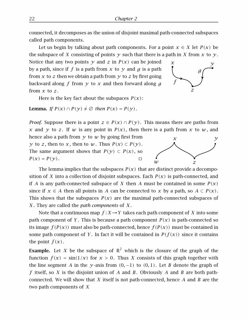
Let us begin by talking about path components. For a point x ∈ X let P(x) be

the subspace of X consisting of points y such that there is a path in X from x to y .

Notice that any two points y and z in P(x) can be joined

by a path, since if f is a path from x to y and g is a path

from x to z then we obtain a path from y to z by first going

backward along f from y to x and then forward along g

from x to z .

Here is the key fact about the subspaces P(x) :

Lemma. If P(x)∩ P(y) 6= ∅ then P(x) = P(y) .

Proof. Suppose there is a point z ∈ P(x) ∩ P(y) . This means there are paths from

x and y to z . If w is any point in P(x) , then there is a path from x to w , and

hence also a path from y to w by going first from

y to z , then to x , then to w . Thus P(x) ⊂ P(y) .

The same argument shows that P(y) ⊂ P(x) , so

P(x) = P(y) . ⊔⊓

The lemma implies that the subspaces P(x) that are distinct provide a decompo-

sition of X into a collection of disjoint subspaces. Each P(x) is path-connected, and

if A is any path-connected subspace of X then A must be contained in some P(x)

since if x ∈ A then all points in A can be connected to x by a path, so A ⊂ P(x) .

This shows that the subspaces P(x) are the maximal path-connected subspaces of

X . They are called the path components of X .

Note that a continuous map f :X→Y takes each path component of X into some

path component of Y . This is because a path component P(x) is path-connected so

its image f(P(x)) must also be path-connected, hence f(P(x)) must be contained in

some path component of Y . In fact it will be contained in P(f(x)) since it contains

the point f(x) .

Example. Let X be the subspace of R2 which is the closure of the graph of the

function f(x) = sin(1/x) for x > 0. Thus X consists of this graph together with

the line segment A in the y -axis from (0,−1) to (0,1) . Let B denote the graph of

f itself, so X is the disjoint union of A and B . Obviously A and B are both path-

connected. We will show that X itself is not path-connected, hence A and B are the

two path components of X

Connectedness 23

Let f : [0,1]→X be a path starting at a point in A . We know that f−1(A) is closed

since A is closed. We will show that f−1(A) is also open. This implies f−1(A) = [0,1]

since [0,1] is connected and f−1(A) is nonempty. The equation f−1(A) = [0,1] says

that f([0,1]) ⊂ A , and thus there is no path in X joining a point in A to a point in B .

To show that f−1(A) is open let t0 be any point in f−1(A) . Choose a small open disk

D in R2 centered at f(t0) . Then D∩X has infinitely many path-components, one of

which is D∩A . Since f is continuous, f−1(D) is an open set in [0,1] containing t0 ,

so there is an interval I ⊂ [0,1] which is open in [0,1] , contains t0 , and is contained

in f−1(D) . This interval is path-connected, so its image f(I) is also path-connected

and therefore lies inside one of the path components of D∩X . This path component

contains the point f(t0) ∈ A so it has to be the path component D ∩ A . This says

that f(I) ⊂ A , or in other words I ⊂ f−1(A) . Thus f−1(A) contains a neighborhood

of t0 in [0,1] . Since t0 was an arbitrary point of f−1(A) we conclude that f−1(A) is

open in [0,1] , finishing the argument.

To determine whether the space X in this example is connected we will use the

following general fact:

Lemma. If a subspace A of a space X is connected, then so is A .

Proof. Suppose A is the disjoint union of subsets B and C which are closed in A and

hence also closed in X since A is closed in X . Then A∩B and A∩C are disjoint closed

sets in A whose union is A , so one of these two sets must equal A , say A ∩ B = A .

This says A ⊂ B , so A ⊂ B = B . Since we originally had A = B∐C this implies B = A

and C = ∅ . ⊔⊓

From this lemma we can conclude that the space X in the preceding example

is connected since it is the closure of the subspace B which is path-connected and

hence connected. Thus X is an example of a space which is connected but not path-

connected. Another example, very similar to this one, would be the closure of the

graph of the function r = ϑ/(ϑ + 1) for ϑ ≥ 0, in polar coordinates. This space

consists of a circle together with a curve that spirals out to it from inside.

Now we turn to the question of decomposing a space X into maximal connected

24 Chapter 2

subspaces.

Lemma. If A is a subset of a space X which is both open and closed, then any connected

subspace C ⊂ X which meets A must be contained in A .

Proof. If A is open and closed in X then C ∩ A is open and closed in C . If C is

connected this implies that C ∩A = C , which says that C is contained in A . ⊔⊓

Proposition. If {Cα} is a family of connected subspaces of a space X , any two of which

have nonempty intersection, then⋃

α Cα is connected.

Proof. Let Y =⋃

α Cα and let A ⊂ Y be open and closed in Y . Then A ∩ Cα is open

and closed in Cα for each α , hence is either ∅ or Cα . If A 6= ∅ choose a point x ∈ A .

Since A ⊂ Y and Y is the union of all the Cα ’s we have x ∈ Cα for some α . Thus

A∩ Cα 6= ∅ , so by the preceding lemma we must have Cα ⊂ A . Any other Cβ meets

Cα by assumption, hence meets A and so is contained in A by the Lemma again. Thus

Y , the union of the Cα ’s, is contained in A . We were assuming A ⊂ Y , so we have

A = Y . Since A was any nonempty closed and open set in Y , we conclude that Y is

connected. ⊔⊓

We can apply the proposition to the collection of all connected subsets Cα of X

that contain a given point x , to conclude that the union of all these subsets is con-

nected. Call this union C(x) . It is obviously the largest connected set in X containing

x since it contains every connected set that contains x . Obviously C(x) is also the

largest connected set containing any other point y ∈ C(x) , since a larger connected

set containing y would also be a larger connected set containing x . It follows that X

is the disjoint union of all the different sets C(x) . These are the maximal connected

sets in X , the connected components of X .

Note that the connected components of X are closed subsets by the earlier fact

that if a subspace A ⊂ X is connected then so is its closure. Connected compo-

nents do not have to be open, however. For example, consider the rational numbers

Q , topologized as a subspace of R . We know from earlier that the only connected

subspaces of R are intervals, including the degenerate intervals [a,a] . Since Q con-

tains no nondegenerate intervals, it follows that the only connected subspaces of Q

are points. Thus the connected components of Q are just the individual points of

Q , since connected components are maximal connected subspaces. The connected

components of Q are therefore not open subsets of Q .

Path components do not have to be either open or closed, as one can see in the

example of the closure of the graph of sin(1/x) . This graph is a path component

Connectedness 25

that is open but not closed, while the remaining line segment of the space is a path

component that is closed but not open.

Each path component of a space is contained in a connected component since

path-connected subspaces are connected, hence are contained in maximal connected

subspaces, the connected components. One commonly encountered situation where

path components are the same as connected components is given by the following

result:

Proposition. If each point in a space X has a neighborhood which is path-connected,

then the path components of X are also the connected components.

Proof. The hypothesis guarantees that path components are open subsets. This im-

plies that they are also closed since the complement of a path component is a union

of path components and hence is open. Any connected set must intersect some path

component and hence be contained in it by the previous lemma, so the connected

components are contained in the path components. ⊔⊓

This proposition applies for example to an open set X in Rn , since each point in

X then has a neighborhood which is a ball, which is path-connected. Notice that the

proposition definitely does not apply to the closure of the sin(1/x) graph.

The Cantor Set

A space X whose connected components are points is said to be totally discon-

nected. This is equivalent to saying that the only connected subspaces of X are points,

since connected components are maximal connected subspaces. As a trivial example,

a space with the discrete topology is certainly totally disconnected since every subset

is open and closed, so no subspace with more than one point can be connected.

For a subspace of R to be totally disconnected means that it contains no intervals,

other than points, since the only connected subspaces of R are intervals. We men-

tioned the example of Q previously, but there are many more totally disconnected

subspaces of R . For a start, one can have subspaces such as the integers where every

point is isolated, being both open and closed. This is just saying that the subspace

topology is the discrete topology, so one has a discrete subspace.

Let us ask the following question: Is there a totally disconnected subspace of

R which is closed in R but contains no isolated points. Such a subspace would thus

combine features of both the integers (a closed subspace) and the rationals (a subspace

26 Chapter 2

with no isolated points). The answer to the question is yes, and there is a famous

example which we will now describe, known as the Cantor set.

The Cantor set C is a subspace of [0,1] constructed as an intersection of an

infinite sequence of sets C0 ⊃ C1 ⊃ C2 ⊃ ··· . We start with C0 = [0,1] , and we form

C1 be removing the open interval (1/3,2/3) , so C1 = [0,1/3] ∪ [2/3,1] . Next we

form C2 by removing the open middle thirds (1/9,2/9) and (7/9,8/9) of the two

intervals of C1 . This leaves the four closed intervals [0,1/9] , [2/9,1/3] , [2/3,7/9] ,

and [8/9,1] . Now we repeat the same process over and over again, at each stage

removing the open middle thirds of each interval created at the previous stage. Thus

Cn consists of 2n closed intervals of length 1/3n . Finally we set C =⋂

n Cn . This is

a closed subset of R , being the intersection of the closed subsets Cn .

The set C is totally disconnected since it was constructed so as to contain no

intervals other than points. Namely, if C contained an interval of positive length ε

then this interval would be contained in each Cn , but Cn contains no interval of length

greater than 1/3n so if n is chosen to be large enough so that 1/3n is less than ε ,

then there is no interval of length ε in Cn .

Now let us check that C contains no isolated points. Each point x in C is in

the intersection of all the Cn ’s so it is in the intersection of the sequence of interval

components In of Cn that contain x . If we let xn be either endpoint of In then

x = limxn since the lengths of the In ’s are approaching 0. We can assume x 6= xn

for all n since we have two choices for each xn so we can always choose one of them

different from x if x happens to be an endpoint of some In . All the endpoints of

the In ’s are contained in C , so this shows that each x ∈ C is a limit of a sequence of

points xn ∈ C different from x . This shows that C contains no isolated points.

There is a nice way of characterizing which points of [0,1] lie in C in terms of

base 3 decimals. The middle-third interval (1/3,2/3) consists of base 3 decimals

.a1a2 ··· with a1 = 1, excluding only the decimal .1 = 1/3. Thus C1 consists of

the decimals .a1a2 ··· with a1 6= 1, including 1/3 as .0222 ··· and 1 as .222 ··· .

In similar fashion C2 consists of decimals .a1a2 ··· with a1 6= 1 and a2 6= 1. More

generally Cn consists of decimals .a1a2 ··· with none of a1, ··· , an equal to 1. Hence

C consists exactly of all decimals .a1a2 ··· with no ai equal to 1. The points of C

that are endpoints of an interval component of some Cn are the decimals ending

either in all 0’s or all 2’s.

It is interesting to think of the process of constructing C in physical terms as

taking a length of string and repeatedly cutting it into shorter pieces. If we think of

the first piece as the interval [0,1] and cut it at the point 1/2, then it becomes two

Connectedness 27

pieces of string each with two endpoints. In effect the single point 1/2 has become two

points, the two new endpoints of the half pieces, the intervals [0,1/2] and [1/2,1] .

At the next stage one cuts each of these two pieces in half, producing four separate

pieces [0,1/4] , [1/4,1/2] , [1/2,3/4] , and [3/4,1] , and so on for later stages. In

order to make all these pieces disjoint subsets of R one can image the string as being

stretched so tightly that each time it is cut, it pulls apart at the cut and shrinks to

two-thirds of its length, so after the first cut, [0,1/2] shrinks to [0,1/3] and [1/2,1]

shrinks to [2/3,1] . Then at the next stage we cut [0,1/3] at its midpoint and the two

pieces [0,1/6] and [1/6,1/3] shrink to [0,1/9] and [2/9,1/3] , and similarly for the

piece [2/3,1] , and so on.

All this cutting and shrinking can be described very neatly in terms of decimal

expansions. Initially we cut [0,1] at 1/2 producing two copies of the point 1/2. If we

use base 2 decimals, then these two copies of 1/2 can be distinguished by regarding

one of them as .0111 ··· and the other one as .1000 ··· . Normally these two decimals

are regarded as the same number, but now we want to keep them distinct, viewing

them as the two new endpoints of the cut string. Similarly at the next stage the point

1/4 duplicates itself as the two decimals .00111 ··· and .01000 ··· , and the point 3/4

duplicates itself as .10111 ··· and .11000 ··· , etc. The process of shrinking pieces to

two-thirds of their lengths can then be achieved by simply changing the decimal base

2 to 3 and replacing all decimal digits 1 by 2.

Here is a question for the reader to ponder: What happens if we do not replace

decimal digits 1 by 2 but simply consider all base 3 decimals consisting of 0’s and

1’s, with no 2’s? How does the resulting set compare with the Cantor set?

We can determine the total length of the Cantor set by adding up the lengths of

the complementary deleted intervals. First we deleted an interval of length 1/3, then

2 intervals of length 1/9, then 4 intervals of length 1/27, and so on. Thus the total

length deleted is the sum of the series13+

29+

427+ ··· , which is a geometric series

with initial term 1/3 and ratio 2/3 so the sum is 1. Thus the total length of C is 0.

Another way to see this is to observe that the length of Cn is 2/3 of the length of

Cn−1 , so the length of Cn is (2/3)n , which approaches 0 as n goes to infinity.

One can imagine many similar constructions of sets that look much like the Can-

tor set. For example, instead of removing middle thirds at each step one could remove

middle halves or middle quarters, or any other fractions. The fractions could even vary

from one step to the next. Or instead of removing a single middle interval from each

interval, one could remove several interior open intervals, provided that the lengths

28 Chapter 2

of the remaining intervals approach zero. Interestingly enough, all these construc-

tions produce ‘Cantor sets’ that are homeomorphic to the original Cantor set C . In

fact, it is possible to list several properties that the Cantor set has, including being

totally disconnected and having no isolated points, such that every space with these

properties is homeomorphic to the Cantor set. We will study the other properties in

the next couple chapters, and eventually (hopefully) prove the theorem that the list

of properties characterizes the Cantor set up to homeomorphism.

Exercises

1. Let D1 and D2 be two open disks in R2 whose closures D1 and D2 intersect in

exactly one point, so the boundary circles of the two disks are tangent. Determine

which of the following subspaces of R2 are connected: (a) D1 ∪ D2 . (b) D1 ∪ D2 .

(c) D1 ∪D2 .

2. Show that if a subspace A of a space X is connected then so is its closure A .

3. Show the subspace X ⊂ R2 consisting of points (x,y) such that at least one of x

and y is rational is connected.

4. By counting cut points and non-cut points show that no two of the following four

graphs in R2 are homeomorphic. (Each graph is a closed subspace of R2 , the union

of a finite number of closed line segments.)

5. Show that if a space X has only a finite number of connected components, then

these components are open subsets of X . (We already know they are closed.)

6. From the fact that an interval [a, b] is connected, deduce the Intermediate Value

Theorem: If f : [a, b]→R is continuous and f(a) < c < f(b) then there exists a

number x ∈ [a, b] with f(x) = c .

7. (a) Show that if A ⊂ B ⊂ A and A is connected then so is B .

(b) Let X ⊂ R2 be the closure of the graph of sin(1/x) for x > 0. Using part (a),

determine all the connected subspaces of X .

Connectedness 29

8. For a space X let X′ be the subspace of X obtained by deleting all points x which

are isolated (i.e. {x} is open and closed in X ). Let Bn be the subspace of [0,1]

consisting of numbers having a base 2 decimal expansion .a1a2 ··· in which at most

n of the digits ai are 1, and let B =⋃

n Bn . Draw a picture of B1 and B2 and

determine B′n and B′ . Deduce that there exist spaces X for which the sequence

X ⊃ X′ ⊃ X′′ ⊃ ··· becomes the empty set only after n stages, for any given number

n .

9. (a) Show that the sets obtained by intersecting the Cantor set C with the interval

components of the spaces Cn form a basis for the topology on C . (Here C =⋂

n Cn .)

(b) Describe the basis sets in part (a) in terms of the base 3 decimal expansions of

elements of C with only 0’s and 2’s.

(c) For each subset S of {1,2, ···} define a function fS :C→C by changing the i -th

digit of a base 3 decimal .a1a2 ··· ∈ C from 0 to 2 or vice versa if i ∈ S and

leaving this digit unchanged if i ∉ S . Using parts (a) and (b), show that fS is a

homeomorphism of C . (Note that f−1S = fS .) Explain why this shows the somewhat

surprising fact that for any two points x,y ∈ C there is a homeomorphism f :C→C

with f(x) = y . In particular, the points of C that are endpoints of intervals of Cn

for some n are no different intrinsically from all the other points of C .

30 Chapter 3

Chapter 3. CompactnessCompactness is a sort of finiteness property that some spaces have and others

do not. The rough idea is that spaces which are ‘infinitely large’ such as R or [0,∞)

are not compact. However, we want compactness to depend just on the topology on

a space, so it will have to be defined purely in terms of open sets. This means that

any space homeomorphic to a noncompact space will also be noncompact, so finite

intervals (a, b) and [a, b) will also be noncompact in spite of their ‘finiteness’. On

the other hand, closed intervals [a, b] will be compact — they cannot be stretched to

be ‘infinitely large’.

How can this idea be expressed just in terms of open sets rather than in some

numerical measure of size? This would seem to be difficult since open sets themselves

can be large or small. But large open sets can be expressed as unions of small open

sets, so perhaps we should think about counting how many small open sets are needed

when a large open set in a space X , such as the whole space X itself, is expressed as

a union of small open sets. The most basic question in this situation is whether the

number of small open sets needed is finite or infinite. For example, if X is a metric

space, then X is the union of all its balls Bε(x) of fixed radius ε > 0, so we could

ask whether X is in fact the union of a finite collection of these balls Bε(x) of fixed

radius. To generalize this idea to arbitrary spaces which need not have a metric, we

replace balls by arbitrary open sets, and this leads to the following general definition:

Definition. A space X is compact if for each collection of open sets Oα in X whose

union is X , there exist a finite number of these Oα ’s whose union is X .

More concisely, one says that every open cover of X has a finite subcover, where

an open cover of X is a collection of open sets in X whose union is X , and a finite

subcover is a finite subcollection whose union is still X .

For example, R is not compact because the cover by the open intervals (−n,n)

for n = 1,2, ··· has no finite subcover, since infinitely many of these intervals are

needed to cover all of R . Another open cover which has no finite subcover is the

collection of intervals (n− 1, n+ 1) for n ∈ Z .

In a similar vein, the interval (0,1) fails to be compact since the cover by the open

intervals (1/n,1) for n ≥ 1 has no finite subcover. Of course, there do exist open

covers of (0,1) which have finite subcovers, for example the cover by (0,1) itself,

or a little less trivially, the cover by all open subintervals of fixed length, say 1/4,

which has the finite subcover (0,1/4) , (1/8,3/8) , (1/4,1/2) , (3/8,5/8) , (1/2,3/4) ,

(5/8,7/8) , (3/4,1) . To be compact means that every possible open cover has a finite

Compactness 31

subcover. This could be difficult to check in individual cases, so we will develop

general theorems to test for compactness.

Compact Sets in Euclidean Space

Spaces with only finitely many points are obviously compact, or more generally

spaces whose topology has only finitely many open sets. However, such spaces are

not very interesting. Our goal in this section will be to characterize exactly which

subspaces of Rn are compact. We start with an important special case:

Theorem. A closed interval [a, b] is compact.

Proof. This will be somewhat similar in flavor to the proof we gave that closed intervals

are connected. The case a = b is trivial, so we may assume a < b . Let a cover of

[a, b] by open sets Oα in [a, b] be given. Since a ∈ Oα for some α , there exists c > a

such that the interval [a, c] is contained in this Oα , and hence [a, c] is contained in

the union of finitely many Oα ’s. Let L be the least upper bound of the set of numbers

c ∈ [a, b] such that [a, c] is contained in the union of finitely many Oα ’s. We know

that L > a by the preceding remarks, and by the definition of L we certainly have

L ≤ b .

There is some Oα , call it Oβ , that contains L . This Oβ is open in [a, b] , so since

L > a there is an interval [L−ε, L] contained in Oβ for some ε > 0. By the definition

of L there exist numbers c < L arbitrarily close to L such that [a, c] is contained

in the union of finitely many Oα ’s. In particular, there are such numbers c in the

interval [L − ε, L] . For such a c we can take a finite collection of Oα ’s whose union

contains [a, c] and add the set Oβ containing [L − ε, L] to this collection to obtain

a finite collection of Oα ’s containing the interval [a, L] . If L = b we would now be

done, so it remains only to show that L < b is not possible.

If L < b , the number ε could have been chosen so that not only is [L−ε, L] ⊂ Oβ

but also [L − ε, L + ε] ⊂ Oβ , since Oβ is open in [a, b] . Then by adding Oβ to the

finite collection of Oα ’s whose union contains [a, c] , as in the preceding paragraph,

we would have a finite collection of Oα ’s whose union contains [a, L+ ε] . However,

this means that L is not an upper bound for the set of c ’s such that [a, c] is contained

in a finite union of Oα ’s. This contradiction shows that L < b is not possible, so we

must have L = b . ⊔⊓

For a subspace A of a space X to be compact means of course that every open

32 Chapter 3

cover of A has a finite subcover. The open cover of A would consist of sets of the

form A∩Oα for Oα open in X . To say that A =⋃

α(A∩Oα) is equivalent to saying

that A ⊂⋃

αOα . Thus for A to be compact means that for every collection of open

sets in X whose union contains A , there is a finite subcollection whose union contains

A . So it does no harm to interpret ‘every open cover of A has a finite subcover’ to

mean precisely this.

Proposition. A closed subset of a compact space is compact, in the subspace topology.

Proof. Let {Oα} be a cover of A by open sets in X . We then obtain an open cover of

X by adding the set X − A , which is open if A is closed. If X is compact this open

cover of X has a finite subcover. The sets Oα in this finite subcover then give a finite

cover of A since the set X −A contributes nothing to covering A . ⊔⊓

As an example, the Cantor set is closed in [0,1] , so it is compact because [0,1]

is compact.

Here is another way to show that a space is compact:

Proposition. If f :X→Y is continuous and onto, and if X is compact, then so is Y .

Proof. Let a cover of Y by open sets Oα be given. Then the sets f−1(Oα) form an

open cover of X . If X is compact, this cover has a finite subcover. Call this finite

subcover f−1(O1), ··· , f−1(On) . Assuming that f is onto, the corresponding sets

O1, ··· ,On then cover Y since for each y ∈ Y there exists x ∈ X with f(x) = y ,

and this x will be in some set f−1(Oi) of the finite cover of X , so y will be in the

corresponding set Oi . ⊔⊓

This implies for example that a circle is compact since it is the image of a contin-

uous map f : [0,1]→R2 .

In order to expand our range of compact spaces we use the notion of product

spaces, introduced in Chapter 1.

Theorem. If X and Y are compact then so is their product X × Y .

By induction this implies that the product of any finite collection of compact

spaces is compact.

Proof. Let a cover of X×Y by open sets Oα in X×Y be given. Each point (x,y) ∈ X×Y

lies in some Oα , and this Oα is a union of basis sets U ×V , so there exists a basis set

Uxy × Vxy containing (x,y) and contained in some Oα .

Compactness 33

Suppose we choose a fixed x and let y vary. Then the sets Uxy × Vxy cover

{x}×Y , so the sets Vxy with fixed x and varying y form an open cover of Y . Since

Y is compact, this cover has a finite subcover Vxy1, ··· , Vxyn , where n may depend

on x . The intersection Ux =⋂nj=1Uxyj is then an open set containing x with two key

properties: The sets Ux × Vxy1, ··· , Ux × Vxyn cover Ux × Y , and each Ux × Vxyj is

contained in some Oα .

Now we let x vary. The sets Ux form an open cover of X , so since X is compact

there is a finite subcover Ux1, ··· , Uxm . The products Uxi ×Vxiyj of the sets Uxi with

the corresponding sets Vxiyj chosen earlier then form a finite cover of X × Y . Each

set in this finite cover is contained in some Oα , so by choosing an Oα containing each

Uxi × Vxiyj we obtain a finite cover of X × Y . ⊔⊓

We can use this result to determine exactly which subspaces of Rn are compact.

The result is usually called the Heine-Borel Theorem.

Theorem. A subspace X ⊂ Rn is compact if and only if it is closed and bounded.

For a subset X ⊂ Rn to be bounded means that it lies inside some ball of finite

radius centered at the origin.

Proof. First let us assemble previously-proved results to show the ‘if’ half of the the-

orem. If we assume X is bounded, then it lies in a ball of finite radius and hence in

some closed cube [−r , r ] × ··· × [−r , r ] . This cube is compact, being a product of

closed intervals which are compact. Since X is a closed subset of a compact space, it

is also compact.

Now for the converse, suppose X is compact. The collection of all open balls in

Rn centered at the origin and of arbitrary radius forms an open cover of X , so there

is a finite subcover, which means X is contained in a single ball of finite radius, the

largest radius of the finitely many balls covering X . Hence X is bounded.

To show X is closed if it is compact, suppose x is a limit point of X that is not

in X . Then every neighborhood of x contains points of X . In particular each open

ball Br (x) of radius r centered at x contains points of X , so the same is true also

for the closed balls Br (x) . The complements Rn−Br (x) form an open cover of X as

r varies over (0,∞) since their union is Rn − {x} and x ∉ X . This open cover of X

has no finite subcover since each Br contains points of X . Thus we have shown that

if X is not closed, it is not compact. ⊔⊓

34 Chapter 3

Hausdorff Spaces

We showed earlier that a compact subspace of Rn is closed. This is not something

that remains true when Rn is replaced by an arbitrary space X . For example if X is

a finite set with any topology then every subspace of X is compact since a cover of

X can have only finitely many sets, but not every subset of X will be closed unless X

has the discrete topology. Fortunately there is a fairly simple and natural condition

to impose on a topology which will guarantee that compact subspaces are closed:

Definition. A topological space X is a Hausdorff space if for each pair of distinct points

x,y ∈ X there exist open neighborhoods U of x and V of y that are disjoint.

For example, every metric space X is a Hausdorff space since if x and y are

distinct points in X then the open balls of radius ε centered at x and y will be

disjoint if ε is less than half the distance between x and y . This follows from the

triangle inequality, since if there were a point z in the intersection of these two balls,

then the distances between x , y , and z would satisfy d(x,y) ≤ d(x, z)+d(z,y) <

ε + ε = 2ε < d(x,y) , a contradiction.

The trivial topology on a space with more than one point is not Hausdorff. A

more interesting example of a non-Hausdorff space is R with the topology having

as its nonempty open sets the complements of finite sets, since in this topology any

two nonempty open sets have a nonempty intersection. Many more examples of non-

Hausdorff spaces can be constructed but they do not arise all that often ‘in nature’.

Most non-Hausdorff spaces are in one way or another artificial. It is probably not a

great exaggeration to say that most interesting spaces are Hausdorff.

Here are three nice properties of Hausdorff spaces:

Proposition. (a) In a Hausdorff space, points are closed subsets.

(b) A subspace of a Hausdorff space is Hausdorff.

(c) A product of two Hausdorff spaces is Hausdorff.

Proof. (a) If X is Hausdorff and x is a point in X , then for any other point y there is

an open neighborhood Vy of y that is disjoint from a neighborhood of x and hence

disjoint from x itself. The union of all these open sets Vy as y ranges over X −{x}

is X − {x} , which is therefore open, so {x} is closed.

(b) Let A be a subspace of X and let x,y ∈ A . If X is Hausdorff these two points

have disjoint open neighborhoods U and V in X , so A ∩ U and A ∩ V are disjoint

open neighborhoods of x and y in A .

Compactness 35

(c) Suppose X and Y are Hausdorff and we have two distinct points (x1, y1) and

(x2, y2) in X × Y , so either x1 6= x2 or y1 6= y2 . In the former case, if U1 and U2

are disjoint neighborhoods of x1 and x2 in X then U1 × Y and U2 × Y are disjoint

neighborhoods of (x1, y1) and (x2, y2) in X × Y . The opposite case y1 6= y2 is

handled similarly. ⊔⊓

Proposition. A compact subspace of a Hausdorff space is closed.

Proof. Let X be Hausdorff with A ⊂ X compact. The main work will be to show that

for each x ∈ X −A there exist disjoint open sets U and V in X such that x ∈ U and

A ⊂ V . This will imply that A is closed since no point x in the complement of A can

be a limit point of A since it has a neighborhood U disjoint from A .

Now we construct U and V with the desired properties. The point x ∈ X−A and

an arbitrary point a ∈ A have disjoint open neighborhoods Ux and Va in X since X

is Hausdorff. As a ranges over A the open sets Va form an open cover of A . Since A

is compact, this open cover has a finite subcover. Call this subcover V1, ··· , Vn , and

let the sets Ux that correspond to these Vi ’s be labelled U1, ··· , Un . The intersection

U = U1 ∩ ··· ∩ Un is an open neighborhood of x that is disjoint from each Vi and

hence also from the union V = V1∪···∪Vn , which is an open set containing A . ⊔⊓

Corollary. A map f :X→Y from a compact space X to a Hausdorff space Y is a

homeomorphism if it is continuous, one-to-one, and onto.

Proof. All that needs to be checked is that f−1 is continuous, and to do this it suffices

to show that if C ⊂ X is closed in X then f(C) is closed in Y . But since C is a closed

subset of a compact space, it is compact, hence f(C) is compact and therefore also

closed since Y is Hausdorff. ⊔⊓

For example, consider continuous maps [0,1]→[0,1] × [0,1] defining paths in

the square. Intuition would suggest that no such map can be onto, but in fact this

intuition is incorrect, and there do exist continuous maps [0,1]→[0,1]×[0,1] whose

image is the whole square. However, no such map can be one-to-one, otherwise the

Corollary would say it is a homeomorphism, but [0,1] and [0,1] × [0,1] are not

homeomorphic since [0,1] has cutpoints but [0,1× [0,1] does not.

The Corollary implies that the topology on a space X that is both compact and

Hausdorff has a certain optimality property. Notice first that any topology that is finer

than a Hausdorff topology is still Hausdorff, while a topology that is coarser than a

compact topology is still compact.

36 Chapter 3

If X is compact and Hausdorff with respect to the topology O , then any other

topology that is strictly finer than O is Hausdorff but not compact, while any

other topology that is strictly coarser than O is compact but not Hausdorff.

To see this, just apply the Corollary to the identity map X→X , which is continuous if

the topology in the domain is finer than the topology in the range. If the topology in

the domain is compact Hausdorff and the topology in the range is strictly coarser, it

would be compact but not Hausdorff, otherwise the Corollary would imply the identity

map was a homeomorphism so the two topologies would be the same. Similarly, if the

topology in the range is compact Hausdorff and the topology in the domain is strictly

finer, it would be Hausdorff but not compact, otherwise the Corollary would say the

identity map was a homeomorphism.

Normal Spaces

Often in a Hausdorff space X there is a stronger form of the Hausdorff condition

that is satisfied: If A and B are disjoint closed sets in X , then there are disjoint open

sets U and V in X with A ⊂ U and B ⊂ V . In short, disjoint closed sets have disjoint

open neighborhoods. A Hausdorff space with this property is called a normal space.

We include the Hausdorff condition as part of the definition of a normal space to

guarantee that points are closed, so that the condition of disjoint closed sets having

disjoint open neighborhoods includes the condition that distinct points have disjoint

open neighborhoods. The reason for restricting A and B to be closed is that one would

not expect arbitrary disjoint subsets to have disjoint open neighborhoods, since for

example in R the sets {0} and (0,1] do not have disjoint open neighborhoods.

In some cases the Hausdorff condition automatically implies normality:

Proposition. A compact Hausdorff space is normal.

Proof. Let A and B be disjoint closed sets in a compact Hausdorff space X . In partic-

ular this implies that A and B are compact since they are closed subsets of a compact

space. By the argument in the proof of the preceding Proposition we know that for

each x ∈ A there exist disjoint open sets Ux and Vx with x ∈ Ux and B ⊂ Vx . Letting

x vary over A , we have an open cover of A by the sets Ux , so there is a finite subcover.

Let U be the union of the sets Ux in this finite subcover and let V be the intersection

of the corresponding sets Vx . Then U and V are disjoint open neighborhoods of A

and B . ⊔⊓

Compactness 37

It is natural to ask whether all Hausdoff spaces are normal, and here is an artifi-

cially constructed example to show that this need not be true:

Example. Let X be the subset of R2 consisting of all points (x,y) with y ≥ 0. We

construct a topology on X that is finer than the usual topology in the following way.

Let X′ ⊂ X be the complement of the x -axis, the points (x,y) with y > 0. Then a

basis for the new topology on X consists first of all of the usual open disks Dr (x) of

radius r and center x that are contained in X′ , and then in addition for each point x

in the x -axis we take the sets D′r (x) = {x}∪(X′∩Dr (x)) obtained by adding x to an

open half-disk centered at x . It is easy to check that the condition for having a basis

is satisfied, and we leave this for the reader to do. The Hausdorff condition is also

easily verified since any two distinct points of X are contained in disjoint basis sets.

Notice that any subset of the x -axis is closed in this topology since its complement is

open, being a union of basis sets. However, if we let A be the rational numbers in the

x -axis and B the irrational numbers, then A and B are disjoint closed sets in X that

do not have disjoint open neighborhoods, since any open set U containing A would

contain basis sets D′r (a) for a ∈ A that intersect all the basis sets D′s(b) for b ∈ B

with |a − b| < r , hence U would intersect any open set V containing B . Thus X is

not normal.

Notice that the subspace topology on the x -axis is the discrete topology since the

intersection of the open set D′r (x) with the x -axis is {x} , making {x} an open set in

this subspace. On the other hand, the subspace topology on X′ , the complement of

the x -axis, is the usual topology. So the topology on X somehow mingles these two

rather different sorts of topologies.

Proposition. Metric spaces are normal.

Before proving this we need a preliminary fact. Let X be a metric space with

metric d . Given a subset A ⊂ X define the distance d(x,A) from a point x ∈ X to

A to the the greatest lower bound of the set of distances d(x,a) from x to points

a ∈ A . Note that d(x,A) ≥ 0, and d(x,A) = 0 if and only if x is in the closure of A

since d(x,A) = 0 is equivalent to saying that every ball Br (x) contains points of A .

Lemma. d(x,A) is a continuous function of x .

Proof. Supposex and y are points in X with d(x,y) < ε . For each δ > 0 there exists

a ∈ A with d(x,a) < d(x,A)+δ . Then d(y,a) < d(y,x)+d(x,a) < ε+δ+d(x,A) .

Since d(y,a) ≤ d(y,A) this implies d(y,A) < ε + δ + d(x,A) . Since δ was any

positive number, it follows that d(y,A) ≤ ε + d(x,A) , or d(y,A) − d(x,A) ≤ ε .

38 Chapter 3

Switching the roles of x and y in this inequality, we have also d(x,A)−d(y,A) ≤ ε ,

so |d(x,A) − d(y,A)| ≤ ε , under the original assumption that d(x,y) < ε . This

implies that d(x,A) is a continuous function of x . ⊔⊓

Proof of the Proposition. If A and B are disjoint closed sets in the metric space X , we

claim that the sets U = {x | d(x,A) < d(x, B) } and V = {x | d(x, B) < d(x,A) } are

disjoint open neighborhoods of A and B , respectively. Certainly they are disjoint, and

they are open since for the difference function d(x,A)−d(x, B) , which is continuous

by the Lemma, U and V are the inverse images of the open sets (−∞,0) and (0,∞) .

To see that A ⊂ U note that d(x,A) = 0 for points x ∈ A and d(x,A) > 0 for point

x ∉ A since A is closed. Similarly we have B ⊂ V using the assumption that B is

closed. ⊔⊓

Lebesgue Numbers

Given a cover of a metric space X by subsets Aα , a Lebesgue number for the

cover is a number ε > 0 such that every ball Bε(x) in X is contained in at least one

set Aα of the cover.

Theorem. Every open cover of a compact metric space X has a Lebesgue number.

For example, what would a Lebesgue number for the following open cover of a

square be?

Proof. Since X is compact, each open cover has a finite subcover, and there is no loss

Compactness 39

of generality to find a Lebesgue number for this subcover. Thus we may assume the

cover is by open sets U1, ··· , Un .

For a ball Bε(x) to be contained in Ui is equivalent to the requirement that

d(x,X − Ui) ≥ ε . Thus we are led to consider the functions di(x) = d(x,X − Ui) ,

and to ask whether there exists an ε > 0 such that for each x ∈ X at least one of the

numbers d1(x), ··· , dn(x) is at least ε . Phrased differently, we are asking whether

there is an ε > 0 such that the function f(x) = max{d1(x), ··· , dn(x)} satisfies

f(x) ≥ ε for all x . Each function di(x) is continuous by the preceding Lemma, and

we leave it as an exercise for the reader to verify that the maximum of a finite set

of continuous functions is again continuous. (By induction it suffices to do the case

of two functions.) So f is continuous. Since Ui is open, its complement X − Ui is

closed and hence di(x) > 0 for all x ∈ Ui . Thus f(x) > 0 for all x ∈ X since the

Ui ’s cover X . Since X is compact, the image f(X) is compact in (0,∞) , so there is a

lower bound ε > 0 for the values of f on X . By the remarks at the beginning of this

paragraph, this ε is a Lebesgue number for the cover. ⊔⊓

Corollary. Let f :X→Y be a continuous map from a compact metric space X to a

metric space Y . Then f is uniformly continuous: For each ε > 0 there exists a δ > 0

such that d(f(x), f (x′)) < ε for all x,x′ ∈ X with d(x,x′) < δ .

Proof. Given ε > 0, cover X by the open sets f−1(Bε/2(y)) as y ranges over Y . Let

δ be a Lebesgue number for this cover of X . Then f takes each ball Bδ(x) to some

ball Bε/2(y) , so if d(x,x′) < δ then d(f(x), f (x′)) ≤ d(f(x),y) + d(y, f (x′)) <

ε/2+ ε/2 = ε . ⊔⊓

Infinite Products

There are times when one is interested in the product X1 × X2 × ··· of an infi-

nite sequence of spaces X1, X2, ··· . As a set, this product consists of all sequences

(x1, x2, ···) with xi ∈ Xi for each i . We will also use the notation∏

iXi for this

product. As an example, the Cantor set can be viewed as the product∏

i Xi where

each Xi is the set {0,2} by identifying an infinite base 3 decimal .a1a2 ··· with the

sequence (a1, a2, ···) .

A first guess for how to define a topology on an infinite product∏

iXi would be

to do the same thing as for finite products, taking as a basis the products U1×U2×···

of open sets Ui ⊂ Xi . The same argument as for finite products shows that this does

40 Chapter 3

in fact define a topology, called the box topology on∏

iXi . However, if one tries to

work with this topology, one finds it has some undesirable features. For example,

many maps Z→∏

i Xi that one would expect to be continuous are not continuous if

the box topology is used on the infinite product. To take a concrete instance, if Z and

each Xi is R then the harmless-looking map x֏ (x,x, ···) fails to be continuous,

since the inverse image of the product (−1/2,1/2)× (−1/3,1/3)× (−1/4,1/4)× ···

is just {0} , which is not open.

Fortunately there is another topology on infinite products that avoids defects

like this. Instead of taking a basis to consist of all products U1 × U2 × ··· of open

sets Ui ⊂ Xi , one only takes products where Ui = Xi for all except finitely many

values of i . This guarantees that a map f :Z→∏

iXi , f(z) = (f1(z), f2(z), ···) , is

continuous if and only if each fi is continuous, since we have f−1(U1 × U2 × ···) =

f−11 (U1)∩ f

−12 (U2)∩ ··· , and this will be open if each fi is continuous, as it is really

only a finite intersection since f−1i (Ui) = f

−1i (Xi) = Z for all but finitely many values

of i .

This topology on∏

iXi is called the product topology since it turns out to be

the one that is used for infinite products almost all the time. Notice that for finite

products it gives the same thing as the product topology defined earlier.

Example. The Cantor set is homeomorphic to the product {0,2} × {0,2} × ··· where

each {0,2} is given the discrete topology. [Proof: Use the basis for the Cantor set

given by the sets O(a1, ··· , an) consisting of all decimals whose first n digits are

a1, ··· , an and whose remaining digits are arbitrary.]

Another advantage of the product topology over the box topology is that it pre-

serves compactness:

Theorem. An infinite product∏∞i=1Xi with the product topology is compact if each Xi

is compact.

This would not be true for the box topology. For example, if each Xi is a finite set

having at least two elements, with the discrete topology, then the box topology on the

infinite product is the discrete topology, which is never compact for an infinite set.

Proof. We will argue by contradiction. Suppose there is an open cover O of∏

iXi that

has no finite subcover. Assuming this, we claim first that there exists a point x1 ∈ X1

such that no basis set U1×X2×X3×··· with x1 ∈ U1 is covered by finitely many sets

in O . For otherwise if for every x1 there was a basis set U1×X2×X3×··· covered by

finitely many sets in O , with x1 ∈ U1 , then the collection of all these U1 ’s as x1 varied

Compactness 41

over X1 would be an open cover of X1 , so since X1 is compact this cover would have

a finite subcover, and it would follow that the cover O had a finite subcover, contrary

to assumption.

Having chosen the point x1 , we claim next that there is a point x2 ∈ X2 such that

no basis set U1×U2×X3×··· with (x1, x2) ∈ U1×U2 is covered by finitely many sets

in O . For otherwise if for every x2 there was such a basis set U1×U2×X3×··· , then

the collection of these U2 ’s as x2 varied over X2 would be an open cover of X2 , and

compactness of X2 would give a finite subcover. Letting U ′1 be the intersection of the

corresponding finite set of U1 ’s, we would then have a basis set U ′1 × X2 × X3 × ···

covered by finitely many sets in O , with x1 ∈ U′1 , contrary to how x1 was chosen in

the preceding paragraph.

Repeating this same argument, we can choose an infinite sequence of points xi ∈

Xi for i = 1,2, ··· , such that for each n , no basis set U1 × ··· × Un × Xn+1 × ···

with (x1, ··· , xn) ∈ U1 × ··· × Un is covered by finitely many sets in O . But this is

impossible because the point (x1, x2, ···) has to lie in some set in O and since this

set is open, it will contain a basis set U1×···×Un×Xn×··· containing (x1, x2, ···) ,

so in particular this basis set will be covered by a single set in O . ⊔⊓

We have considered the product of a countable collections of spaces Xn but it

is also possible to define the product of an arbitrary infinite collection of spaces Xα

where α ranges over any index set I . If I is uncountable we cannot write elements

of the product∏

αXα as sequences (x1, x2, ···) . Instead, elements of∏

αXα are

regarded as functions α֏ xα ∈ Xα , assigning an element of Xα to each index α ,

just as sequences (x1, x2, ···) can be viewed as functions i֏ xi ∈ Xi . One can

write an element of∏

αXα briefly as (xα) , it being understood that this is not just a

single xα but a family of them parametrized by α ∈ I . As in the case of countable

products, the product topology on∏

αXα has as basis the products∏

αUα of open

sets Uα ⊂ Xα such that Ua = Xα for all but finitely many values of α . It is again a

theorem that∏

αXα is compact if each Xα is compact, but the proof requires a fancier

form of induction that depends on a preliminary discussion of set theory topics called

the ‘well-ordering principle’ and the ‘axiom of choice’, so we will not go into this here.

Exercises

1. Give a detailed proof that if two spaces are homeomorphic and one of them is

compact, then so is the other.

42 Chapter 3

2. Show that a space X is compact if and only if it has the following property: For every

collection of closed sets Cα in X such that the intersection of every finite subcollection

of Cα ’s is nonempty, the intersection of all the Cα ’s is nonempty. [Hint: just use the

fact the closed sets are complements of open sets.]

3. Let X be the real numbers with the topology in which the open sets are the com-

plements of finite sets (and ∅ ). Show that X is compact.

4. Show that if X is compact and f :X→R is continuous, then f is bounded and

takes on a minimum and a maximum value.

5. Show that if f :X→Y is continuous and one-to-one and if Y is Hausdorff then so

is X .

6. Show that if A and B are compact subspaces of a space X , then so is A∪ B . If in

addition X is Hausdorff, show that A∩ B is compact.

7. For subspaces A ⊂ X and B ⊂ Y show that A× B = A × B and int(A × B) =

int(A)× int(B) .

8. Show that [0,1)×[0,1) is homeomorphic to [0,1]×[0,1) but not to [0,1]×[0,1] .

9. Consider the orthogonal group O(n) consisting of all n×n orthogonal matrices,

i.e., n×n matrices whose columns form an orthonormal basis v1, ··· , vn for Rn . We

put a topology on O(n) by regarding it as a subspace of Rn2

, taking the n2 entries

of a matrix in O(n) as the n2 coordinates of a point in Rn2

. (a) Show that O(n)

is a closed subset of Rn2

by considering the dot products vi · vj of the columns of

matrices in O(n) as functions Rn2

→R . (b) Show that O(n) is compact.

10. Consider the function f :S1→S1× S1 given by f(θ) = (2θ,3θ) where we think

of points in S1 as angles θ . Show that f is a homeomorphism onto its image, and

draw a picture of this image on the torus S1 × S1 .

11. Let X be the subset of R2 which is the union of the line segments Ln from (0,0)

to (1,1/n) for n = 1,2, ··· , together with the limiting segment L∞ from (0,0) to

(1,0) . Define a topology on X by saying that a set O ⊂ X is open if O ∩ Ln is open

in Ln for all n , including n = ∞ . (Here Ln is given the subspace topology from R2 .)

(a) Show the axioms for a topology are satisfied.

(b) Find a set that is open in this topology but not in the topology on X as a subspace

of R2 .

(c) Show that X is not compact in this new topology, in contrast with the subspace

topology where it is compact since it is a closed bounded subset of R2 .

Compactness 43

12. For a set X define d :X×X→R by setting d(x,x) = 0 and d(x,y) = 1 if x 6= y .

Show that d is a metric. What is the topology defined by this metric?

13. (a) Given a metric d on a set X , show that each of the functions d′(x,y) listed

below is again a metric, and that d and d′ define the same topology on X . Note that

in (b) and (c) the values of d′ are bounded above by 1.

(a) d′(x,y) = kd(x,y) for any constant k > 0.

(b) d′(x,y) =min{d(x,y),1} .

(c) d′(x,y) = d(x,y)/(1+ d(x,y)) .

14. For a metric space X defined by a metric d show that the function d :X ×X→R

is continuous.

15. Let X be a metric space with metric d . For subsets A,B ⊂ X define d(A,B) =

inf{d(a,b) | a ∈ A and b ∈ B } . Show that if A and B are compact then there exist

points a ∈ A and b ∈ B with d(a,b) = d(A,B) , so in particular d(A,B) > 0 if

A∩ B = ∅ . Show by an example that both these statements can be false if A and B

are only assumed to be closed instead of compact.

16. Let X be the subset of R2 which is the union of the line segments Ln from (0,0)

to (1,1/n) for n = 1,2, ··· , together with the limiting segment L∞ from (0,0) to

(1,0) . Define a topology O on X by saying that a set O ⊂ X is in O if O∩Ln is open

in Ln for each n ≤ ∞ , where Ln is given the subspace topology from R2 . Show that

this topology on X is normal but is not defined by any metric on X . Hint: Given a

metric on X , find a sequence of points xn ∈ Ln , n = 1,2, ··· , converging to (0,0) in

the topology defined by the metric but not in the topology O .

44 Chapter 4

Chapter 4. Quotient Spaces

Our next objective is to describe a general procedure for building complicated

spaces out of simpler spaces. This is the topological analog of how all sorts of objects

are made in the real world. Just think of all the different words there are in the En-

glish language for putting things together: gluing, pasting, taping, stapling, stitching,

sewing, welding, riveting, soldering, brazing, bonding, nailing, bolting, clamping, ...

To take two simple examples, we can construct either a cylinder or a Mobius band

by taking a rectangular strip and gluing two opposite edges together:

The gluing process can be described as a map f :X→Y where X is the rectangle and

Y is either the cylinder or the Mobius band. The map f is onto, but not quite one-

to-one because of the gluing: Two points on opposite edges of the rectangle that are

glued together have the same image under f , but other than this, f is one-to-one.

Is it possible to describe the topology on Y just in terms of the topology on X

and the map f ? If so, then we can construct the space Y just by saying “start with

the space X and glue this to that", since the gluing instructions are telling what the

set Y and the map f are. In many cases there is an easy way to characterize open

sets in Y in terms of open sets in X :

Proposition. If f :X→Y is continuous and onto, with X compact and Y Hausdorff,

then a set U ⊂ Y is open in Y if and only if f−1(U) is open in X .

Proof. Continuity of f says that f−1(U) is open if U is open, so we need to see that

the converse is true if X is compact and Y is Hausdorff. If f−1(U) is open in X then

X−f−1(U) is closed and hence compact since X is compact. The image f(X−f−1(U))

is then compact in Y , and therefore also closed since Y is Hausdorff. But since f is

onto we have f(X − f−1(U)) = Y −U . Thus Y −U is closed, so U is open. ⊔⊓

Quotient Spaces 45

This Proposition applies to the cylinder and Mobius band examples. One’s first

guess might have been that the open sets in Y are the images f(O) of open sets O

in X . However, this isn’t right because an open neighborhood of a point x on the left

or right edge of the rectangle is sent to a set in Y that is not an open neighborhood

of f(x) , but only ‘half’ of an actual open neighborhood U of f(x) . To get the other

half of U one would have to enlarge the open set O in X to include also an open

neighborhood of the other point x′ with f(x′) = f(x) . This amounts to replacing O

by f−1(U) , as stated in the Proposition.

The previous Proposition gives a characterization of the topology on Y in terms

of the topology on X , assuming that the topology on Y is already given. It is also

possible to make this characterization into a definition of a topology on Y , as the

following shows:

Proposition. Given a space X , a set Y , and a function f :X→Y , then the collection of

all sets U ⊂ Y such that f−1(U) is open in X is a topology on Y .

Proof. The axioms for unions and intersections are satisfied since f−1(⋃

αUα) =⋃

α f−1(Uα) and f−1(

⋂

αUα) =⋂

α f−1(Uα) . For the other two axioms we have

f−1(∅) = ∅ and f−1(Y ) = X . ⊔⊓

Notice that we did not require f to be onto in this Proposition. If f is not onto

then points y ∈ Y −f(X) form open sets {y} since their inverse images f−1(y) are

empty and hence open. So these points are just isolated points of Y having nothing

to do with the topology on f(X) . Assuming f is onto is thus not a very serious

restriction.

Definition. If the map f :X→Y is onto, the topology on Y given by this Proposition

is called the quotient topology on Y , and the map f is called a quotient map. One also

says that Y is a quotient space of X .

In these terms, the earlier Proposition then says that any continuous map from a

compact space to a Hausdorff space that is onto is a quotient map.

In the examples of the torus and Mobius band as quotient spaces of a rectangle

we already had existing models of the quotient space, but sometimes one wants to

46 Chapter 4

construct a quotient space without having a model of it available beforehand. One

would just like to start with a space X and say “glue this to that" and know that these

instructions will automatically produce a quotient space of X . To see that this is

always possible, suppose first that we do have a quotient map f :X→Y . The points

of X that are ‘glued together’ to produce a point y ∈ Y are exactly the points in

f−1(y) . Since quotient maps are onto, f−1(y) is always nonempty. Thus the points

y ∈ Y are in one-to-one correspondence with the subsets f−1(y) of X . These subsets

are disjoint for different choices of y , and their union is all of X since each point of

X is sent by f to some point of Y . Thus the sets f−1(y) form a partition of X into

disjoint subsets. For example, for the cylinder and Mobius band these subsets of the

rectangle each have either one or two points — either a pair of points on the left and

right edges of the rectangle or a single point not on either of these edges.

Conversely, suppose we are given a partition of X into disjoint nonempty subsets.

For x ∈ X we denote the set in the partition containing x by [x] . If we simply define

Y to be the set of all these subsets [x] , then we have a natural function f :X→Y

sending x to [x] , and this f is onto so we can use it to define a topology on Y by

specifying that a set U ⊂ Y is open exactly when f−1(U) is open in X . This makes f

into a quotient map. We will use the notation X/ ∼ for this quotient space Y whose

points are the sets [x] in the partition of X . Here ∼ is the relation on X given by

x ∼ x′ if [x] = [x′] , i.e., x and x′ lie in the same set in the partition of X . This is

an equivalence relation, meaning that it satisfies the three properties

(i) x ∼ x for all x ∈ X .

(ii) If x ∼ y then y ∼ x .

(iii) If x ∼ y and y ∼ z then x ∼ z .

Conversely, every equivalence relation on X determines a partition of X into the

equivalence classes [x] = {x′ ∈ X | x′ ∼ x } .

In practice the partition of X is often specified implicitly by saying which points

we wish to glue together, or in other words, which points of X we wish to become

identified to single points in Y . For example, to obtain the cylinder from the rectangle

[0,1]× [0,1] we make the identifications (0, t) ∼ (1, t) for t ∈ [0,1] , and to obtain

the Mobius band we instead identify (0, t) ∼ (1,1 − t) . If identifications in a space

X are specified by means of a relation ∼ then this determines a quotient space X/ ∼

associated to the partition of X into the smallest subsets that contain all the specified

pairs x ∼ x′ . In particular, if no identifications are specified for a point x ∈ X then

x becomes a set [x] = {x} of the partition all by itself.

Quotient Spaces 47

Example. The torus S1×S1 can be realized as a quotient space of a rectangle [0,1]×

[0,1] by identifying both pairs of opposite edges via (0, t) ∼ (1, t) and (s,0) ∼ (s,1) .

If we first identify the top and bottom edges of the rectangle we obtain a cylinder,

and then identifying the two ends of the cylinder produces a torus. Notice that the

identifications of opposite edges of the rectangle force all four corners to be identified

to a single point. In particular, we are making the identification (0,0) ∼ (1,1) even

though this is not part of either of the original identifications (0, t) ∼ (1, t) and

(s,0) ∼ (s,1) , but follows since (0,0) ∼ (0,1) ∼ (1,1) .

Given a concrete quotient map f :X→Y we can also form the abstract quotient

space X/ ∼ associated to the partition of X into the subsets f−1(y) , and it would

be nice to know that this is really the same as Y . The map f induces a well-defined

function f :X/ ∼→Y sending f−1(y) to y , and this f is obviously one-to-one and

onto.

Proposition. This function f :X/ ∼→Y is a homeomorphism.

Proof. Let p :X→X/ ∼ be the quotient map x֏ [x] = {x′ ∈ X | f(x′) = f(x) } , so

f = fp . Then a set U ⊂ Y is open if and only if f−1(U) is open (since f is a quotient

map), but since f−1(U) = p−1(f−1(U)) and p is a quotient map, this is equivalent to

f−1(U) being open. ⊔⊓

Example. Let us describe three ways to obtain the sphere S2 as a quotient space. First,

as shown in the figure below, we can form S2 from two closed disks by identifying

their boundary circles together to form a single circle, the equator of S2 . The two

disks then become the upper and lower hemispheres of S2 . More formally, we can

take the two disks as the space X = D2 × {−1,1} ⊂ R2 × R = R3 , where D2 is the

closed unit disk in R2 , and then the identifications are (x,1) ∼ (x,−1) for x ∈ ∂D2 ,

with the map X→S2 given by vertical projection of each disk onto the hemisphere it

is tangent to.

48 Chapter 4

A second way to realize S2 as a quotient space is to start with a single closed disk

D2 and glue the top half of its boundary circle to the bottom half, each point in the

upper half being identified with the point directly below it in the lower half.

Parallel vertical lines in the disk then become parallel vertical circles in S2 . It would

not be difficult to write down a formula for an explicit quotient map D2→S2 that

does this, although there is really no need for explicit formulas.

The third construction also realizes S2 as a quotient of D2 , but this time all the

points of ∂D2 are identified to a single point of S2 , the south pole. This is achieved

by a map D2→S2 that sends each radial line segment to a meridian of S2 going from

the north pole to the south pole. We can view this as taking a disk tangent tangent to

the sphere and wrapping it completely around the sphere.

This example differs from all the previous ones in that the map f :X→Y is no longer

finite-to-one.

Quotient Spaces 49

In the next example we will not have a ready-made model of the quotient space,

so we will be constructing a new space as a quotient of a known space.

Example. Let us construct a surface, commonly called the Klein bottle, by modifying

the earlier construction of the torus from a rectangle by reversing the orientation of

one of the edges of the rectangle:

By definition, the Klein bottle is the quotient space of the rectangle obtained by identi-

fying opposite edges according to the orientations shown. We will use the notation K2

for this space, the superscript indicating that it is a 2-dimensional surface. Identify-

ing the top and bottom edges of the rectangle gives a cylinder, but to identify the two

ends of the cylinder by deforming the cylinder in R3 requires that the cylinder pass

through itself in order to make the orientations match, as in the third figure. Thus we

have a map from K2 into R3 which is not one-to-one because two circles in K2 have

the same image circle C in R3 . In fact, it is a theorem that there is no embedding

of K2 into R3 , i.e., there is no subspace of R3 homeomorphic to K2 . However, there

is an embedding into R4 . The first three coordinates of this embedding are the map

K2→R3 indicated in the figure. For the fourth coordinate we

just need a map f :K2→R that takes different values on the

two circles C1 and C2 of K2 that map to C . In the rectangle

these two circles are positioned as in the figure at the right. We

can choose f to have a value ε > 0 on C1 and be 0 everywhere

outside a small neighborhood of C1 .

Example. Let P2 be the set of all lines through the origin in R3 . This is a metric space

if we define the ‘distance’ between two lines through the ori-

gin to be the smaller of the two angles between them, so this

angle lies in the interval [0, π/2] . The first two properties

required of a metric are obviously satisfied, and we will leave

it for the reader to check the triangle inequality. There is a

natural map p :S2→P2 sending a point x ∈ S2 to the line through the origin con-

taining x . Each line through the origin intersects S2 in two antipodal points x and

50 Chapter 4

−x , so p is onto and is exactly two-to-one. We can see that p is continuous since

p−1 of an ε -ball in P2 consists of two antipodalε -balls in S2 . It follows that p is a

quotient map since it is a continuous map from a compact space onto a Hausdorff

space (metric spaces are Hausdorff). ThIs means that we can regard P2 as the quo-

tient space of S2 in which each point x is identified with the antipodal point −x , so

P2 = S2/(x ∼ −x) .

The classical name for P2 is the projective plane. This comes from thinking of

how 2-dimensional pictures (drawings or paintings, for example) of 3-dimensional

objects are obtained. Each point of a 3-dimensional object projects onto the plane

of the picture along the line from the point to the viewer’s eye. The points that we

see are then really just all the different lines converging to our eye. Normally one’s

angle of vision is something less than 180 degrees, and a picture encompasses con-

siderably less than 180 degrees. But imagine what might happen if we could see more

than 180 degrees at a time. Two points in space that were exactly 180 degrees apart

would presumably be recognized as distinct points. So perhaps if we were making

a mathematical model of how we see things we should not identify antipodal points

of S2 but just consider S2 itself. This leads to a kind of geometry called spherical

geometry. The other alternative of identifying antipodal points leads to a slightly dif-

ferent geometry called projective geometry, which is in some ways closer to Euclidean

geometry, and therefore preferable for some purposes.

Each line through the origin in R3 intersects the upper hemisphere of S2 in either

one or two points, the latter possibility holding only for lines in the xy -plane. This

means that we can also describe P2 as the quotient space of the upper hemisphere

obtained by identifying antipodal points in its boundary, the equator. Since the upper

hemisphere is homeomorphic to a disk via vertical projection onto the unit disk in

the xy -plane, this means that P2 is describable as the quotient space of the disk D2

with the identifications x ∼ −x for x ∈ ∂D2 .

As with the Klein bottle, it is impossible to embed P2 as a subspace of R3 , so one

looks instead for a map P2→R3 that is almost an embedding. We will describe a map

that is an embedding on the interior of D2 and folds the circle ∂D2/(x ∼ −x) onto a

line segment. The image of this map is shown in the figure on the right below:

Quotient Spaces 51

To describe the construction in words, we first deform the D2 in the figure on the left

so that it becomes a sphere with a slit. The boundary circle of the slit is divided into

four arcs and we would like to identify these four arcs in pairs, a with a and b with b

according to the orientations shown. Identifying the first pair presents no problems,

but to identify the second pair then forces all four arcs to coincide in R3 , so that one

has a sphere pinched along a line segment as the image of the map P2→R3 . The

preimage of the interior of this line segment consists of two distinct open arcs in P2 .

The upper half of the third figure is known as a crosscap. It is the image of a

map of a Mobius band to R3 , the Mobius band obtained by removing an open disk

from P2 . Thinking of P2 as D2 with antipodal boundary points identified, the Mobius

band is obtained by removing a smaller concentric disk from D2 , leaving an annulus,

with antipodal points on one of its boundary circles identified. Thinking of P2 as

S2/(x ∼ −x) , one first removes symmetric disk neighborhoods of the two poles of S2

leaving an equatorial band, and then one identifies antipodal points in this band to

produce a Mobius band.

This example of the projective plane easily generalizes to higher dimensions. The

n -dimensional projective space Pn is the space of lines through the origin in Rn+1 ,

the quotient space Sn/(x ∼ −x) , or equivalently the quotient of Dn with antipodal

points of ∂Dn identified. When n = 1 this is just identifying the endpoints of a

semicircle, so P1 is homeomorphic to S1 .

It can easily happen that a quotient space of a Hausdorff space is non-Hausdorff.

Here is a simple example:

Example. Let X = R × {0,1} , two disjoint copies of R , and make the identifications

(x,0) ∼ (x,1) for all x > 0. Then the two points

x0 = (0,0) and x1 = (0,1) are distinct in the quo-

tient although any two neighborhoods U0 of x0 and

U1 of x1 in the quotient intersect since they contain points (x,0) ∼ (x,1) for x > 0.

52 Chapter 4

Quotient maps are not generally open maps, taking open sets to open sets, but this

happens to be the case in this example.

If we make a small modification of this example

by setting (x,0) ∼ (x,1) for x ≥ 0 rather than

x > 0 then the quotient becomes Hausdorff, three

lines in R2 meeting at a point.

Here is a technical result that is used quite often when proving things about

quotient spaces:

Lemma. Given a quotient map f :X→Y and a space Z , then a function g :Y→Z is

continuous if and only if the composition gf :X→Z is continuous.

Proof. Let O ⊂ Z be open. Then by the definition of a quotient map, the set g−1(O)

is open in Y if and only if f−1(g−1(O)) = (gf)−1(O) is open in X . This is saying

that g is continuous if and only if gf is continuous. ⊔⊓

Exercises

For the following problems recall that a map f :X→Y is a quotient map if it is onto

and has the property that a set O ⊂ Y is open if and only if f−1(O) is open in X .

1. Show that a continuous map f :X→Y is a quotient map if there exists a continuous

map g :Y→X such that the composition fg :Y→Y is the identity map. Apply this

to show that a projection map X × Y→X , (x,y)֏ x , is a quotient map.

2. Show that the composition of two quotient maps is a quotient map.

3. Show that there exist quotient maps D2→S1 , S2→D2 , S2→S1 , S2→S1×S1 , and

S1 × S1→S2 . [You do not need to give formulas for these maps, a precise geometric

description will be sufficient. Careful proofs of continuity are not required, but the

quotient maps do have to be continuous. Remember that S1 × S1 is a torus.]

4. (a) Show that there is a quotient map (0,1)→[0,1] , but not [0,1]→(0,1) .

(b) If C is the Cantor set, show there is a quotient map C→[0,1] but not [0,1]→C .

notes on introductory point-set topology

Documents