notes on optimal control theory - …calogero/pdf/note_optimal_control.pdf · notes on optimal...
TRANSCRIPT

NOTES ON OPTIMAL CONTROL THEORY
with economic models and exercises
Andrea CalogeroDipartimento di Matematica e Applicazioni – Universita di Milano-Bicocca
May 14, 2018

ii
Contents
1 Introduction to Optimal Control 11.1 Some examples . . . . . . . . . . . . . . . . . . . . . . . . . . . . 11.2 Statement of problems of Optimal Control . . . . . . . . . . . . . 5
1.2.1 Admissible control and associated trajectory . . . . . . . 51.2.2 Optimal Control problems . . . . . . . . . . . . . . . . . . 9
2 The simplest problem of OC 112.1 The necessary condition of Pontryagin . . . . . . . . . . . . . . . 11
2.1.1 The proof in a particular situation . . . . . . . . . . . . . 152.2 Sufficient conditions . . . . . . . . . . . . . . . . . . . . . . . . . 182.3 First generalizations . . . . . . . . . . . . . . . . . . . . . . . . . 21
2.3.1 Initial/final conditions on the trajectory . . . . . . . . . . 212.3.2 On minimum problems . . . . . . . . . . . . . . . . . . . . 22
2.4 The case of Calculus of Variation . . . . . . . . . . . . . . . . . . 222.5 Examples and applications . . . . . . . . . . . . . . . . . . . . . . 24
2.5.1 The curve of minimal length . . . . . . . . . . . . . . . . 282.5.2 A problem of business strategy I . . . . . . . . . . . . . . 282.5.3 A two-sector model . . . . . . . . . . . . . . . . . . . . . . 312.5.4 A problem of inventory and production I. . . . . . . . . . 33
2.6 Singular and bang-bang controls . . . . . . . . . . . . . . . . . . 362.6.1 The building of a mountain road: a singular control . . . 37
2.7 The multiplier as shadow price I: an exercise . . . . . . . . . . . 40
3 General problems of OC 433.1 Problems of Bolza, of Mayer and of Lagrange . . . . . . . . . . . 433.2 Problems with fixed or free final time . . . . . . . . . . . . . . . . 44
3.2.1 Fixed final time . . . . . . . . . . . . . . . . . . . . . . . . 443.2.2 Free final time . . . . . . . . . . . . . . . . . . . . . . . . 463.2.3 The proof of the necessary condition . . . . . . . . . . . . 483.2.4 The moonlanding problem . . . . . . . . . . . . . . . . . . 50
3.3 The Bolza problem in Calculus of Variations. . . . . . . . . . . . 553.3.1 Labor adjustment model of Hamermesh. . . . . . . . . . . 57
3.4 Existence and controllability results. . . . . . . . . . . . . . . . . 583.4.1 Linear time optimal problems . . . . . . . . . . . . . . . . 62
3.5 Time optimal problem . . . . . . . . . . . . . . . . . . . . . . . . 643.5.1 The classical example of Pontryagin and its boat . . . . . 663.5.2 The Dubin car . . . . . . . . . . . . . . . . . . . . . . . . 69
3.6 Infinite horizon problems . . . . . . . . . . . . . . . . . . . . . . 73
iii

3.6.1 The model of Ramsey . . . . . . . . . . . . . . . . . . . . 763.7 Current Hamiltonian . . . . . . . . . . . . . . . . . . . . . . . . . 79
3.7.1 A model of optimal consumption with log–utility I . . . . 82
4 Constrained problems of OC 854.1 The general case . . . . . . . . . . . . . . . . . . . . . . . . . . . 854.2 Pure state constraints . . . . . . . . . . . . . . . . . . . . . . . . 89
4.2.1 Commodity trading . . . . . . . . . . . . . . . . . . . . . 924.3 Isoperimetric problems in CoV . . . . . . . . . . . . . . . . . . . 96
4.3.1 Necessary conditions with regular constraints . . . . . . . 974.3.2 The multiplier ν as shadow price . . . . . . . . . . . . . . 994.3.3 The foundation of Cartagena . . . . . . . . . . . . . . . . 1004.3.4 The Hotelling model of socially optimal extraction . . . . 101
5 OC with dynamic programming 1055.1 The value function: necessary conditions . . . . . . . . . . . . . . 105
5.1.1 The final condition on V : an first necessary condition . . 1065.1.2 Bellman’s Principle of optimality . . . . . . . . . . . . . . 107
5.2 The Bellman-Hamilton-Jacobi equation . . . . . . . . . . . . . . 1085.2.1 Necessary condition of optimality . . . . . . . . . . . . . . 1085.2.2 Sufficient condition of optimality . . . . . . . . . . . . . . 1115.2.3 Affine Quadratic problems . . . . . . . . . . . . . . . . . . 113
5.3 Regularity of V and viscosity solution . . . . . . . . . . . . . . . 1155.3.1 Viscosity solution . . . . . . . . . . . . . . . . . . . . . . . 118
5.4 More general problems of OC . . . . . . . . . . . . . . . . . . . . 1215.4.1 On minimum problems . . . . . . . . . . . . . . . . . . . . 122
5.5 Examples and applications . . . . . . . . . . . . . . . . . . . . . . 1235.5.1 A problem of business strategy II . . . . . . . . . . . . . . 1285.5.2 A problem of inventory and production II. . . . . . . . . . 130
5.6 The multiplier as shadow price II: the proof . . . . . . . . . . . . 1355.7 Infinite horizon problems . . . . . . . . . . . . . . . . . . . . . . 138
5.7.1 Particular infinite horizion problems . . . . . . . . . . . . 1415.7.2 A model of consumption with HARA–utility . . . . . . . 1415.7.3 Stochastic consumption: the idea of Merton’s model . . . 1445.7.4 A model of consumption with log–utility II . . . . . . . . 144
5.8 Problems with discounting and salvage value . . . . . . . . . . . 1465.8.1 A problem of selecting investment . . . . . . . . . . . . . 147
iv

Chapter 1
Introduction to OptimalControl
1.1 Some examples
Example 1.1.1. The curve of minimal length and the isoperimetric prob-lemSuppose we are interested to find the curve of minimal length joining two distinctpoints in the plane. Suppose that the two points are (0, 0) and (a, b). Clearlywe can suppose that a = 1. Hence we are looking for a function x : [0, 1] → Rsuch that x(0) = 0 and x(1) = b.The length of such curve is defined by∫ 1
0ds, i.e. as the “sum” of arcs of in-
finitesimal length ds; using the pictureand the Theorem of Pitagora we obtain
( ds)2 = ( dt)2 + ( dx)2
⇒ ds =√
1 + x2 dt,
where x = dx(t)dt .
x
1
t
ds
t+dtt
x+dx
x
b
Hence the problem is minx
∫ 1
0
√1 + x2(t) dt
x(0) = 0x(1) = b
(1.1)
It is well known that the solution is a line. We will solve this problem insubsection 2.5.1.
A more complicate problem is to find the closed curve in the plane of assignedlength such that the area inside such curve is maximum: we call this problemthe foundation of Cartagena.1 This is the isoperimetric problem. Without loss
1When Cartagena was founded, it was granted for its construction as much land as a mancould circumscribe in one day with his plow: what form should have the groove because itobtains the maximum possible land, being given to the length of the groove that can dig a manin a day? Or, mathematically speaking, what is the shape with the maximum area among allthe figures with the same perimeter?
1

2 CHAPTER 1. INTRODUCTION TO OPTIMAL CONTROL
of generality, we consider a curve x : [0, 1] → R such that x(0) = x(1) = 0.
Clearly the area delimited by the curve and the t axis is given by∫ 1
0x(t) dt.
Hence the problem is
maxx
∫ 1
0
x(t) dt
x(0) = 0x(1) = 0∫ 1
0
√1 + x2(t) dt = A > 1
(1.2)
Note that the length of the interval [0, 1] is exactly 1 and, clearly, it is reasonableto require A > 1. We will present the solution in subsection 4.3.3.
Example 1.1.2. A problem of business strategyA factory produces a unique good with a rate x(t), at time t. At every moment,such production can either be reinvested to expand the productive capacityor sold. The initial productive capacity is α > 0; such capacity grows as thereinvestment rate. Taking into account that the selling price is constant, whatfraction u(t) of the output at time t should be reinvested to maximize total salesover the fixed period [0, T ]?Let us introduce the function u : [0, T ]→ [0, 1]; clearly, if u(t) is the fraction ofthe output x(t) that we reinvest, (1 − u(t))x(t) is the part of x(t) that we sellat time t at the fixed price P > 0. Hence the problem is
maxu∈C
∫ T
0
(1− u(t))x(t)P dt
x = uxx(0) = α,C = u : [0, T ]→ [0, 1] ⊂ R, u ∈ KC
(1.3)
where α and T are positive and fixed. We will present the solution in subsection2.5.2 and in subsection 5.5.1.
Example 1.1.3. The building of a mountain roadThe altitude of a mountain is given by a differentiable function y, with y :[t0, t1] → R. We have to construct a road: let us determinate the shape ofthe road, i.e. the altitude x = x(t) of the road in [t0, t1], such that the slopeof the road never exceeds α, with α > 0, and such that the total cost of theconstruction ∫ t1
t0
(x(t)− y(t))2 dt
is minimal. Clearly the problem isminu∈C
∫ t1
t0
(x(t)− y(t))2 dt
x = uC = u : [t0, t1]→ [−α, α] ⊂ R, u ∈ KC
(1.4)
where y is an assigned and continuous function. We will present the solution insubsection 2.6.1 of this problem introduced in chapter IV in [22].

1.1. SOME EXAMPLES 3
Example 1.1.4. “In boat with Pontryagin”.Suppose we are on a boat that at time t0 = 0 has distance d0 > 0 from the pierof the port and has velocity v0 in the direction of the port. The boat is equippedwith a motor that provides an acceleration or a deceleration. We are lookingfor a strategy to arrive to the pier in the shortest time with a “soft docking”,i.e. with vanishing speed in the final time T.We denote by x = x(t) the distance from the pier at time t, by x the velocity ofthe boat and by x = u the acceleration (x > 0) or deceleration (x < 0). In orderto obtain a “soft docking”, we require x(T ) = x(T ) = 0, where the final time Tis clearly unknown. We note that our strategy depends only on our choice, atevery time, on u(t). Hence the problem is the following
minu∈C
T
x = ux(0) = d0x(0) = v0x(T ) = x(T ) = 0C = u : [0,∞)→ [−1, 1] ⊂ R
(1.5)
where d0 and v0 are fixed and T is free.This is one of the possible ways to introduce a classic example due to Pon-
tryagin; it shows the various and complex situations in the optimal controlproblems (see page 23 in [22]). We will solve this problem in subsection 3.5.1.4
Example 1.1.5. A model of optimal consumption.Consider an investor who, at time t = 0, is endowed with an initial capital x(0) =x0 > 0. At any time he and his heirs decide about their rate of consumptionc(t) ≥ 0. Thus the capital stock evolves according to
x = rx− c
where r > 0 is a given and fixed rate to return. The investor’s time utility forconsuming at rate c(t) is U(c(t)). The investor’s problem is to find a consumptionplain so as to maximize his discounted utility∫ ∞
0
e−δtU(c(t))dt
where δ, with δ ≥ r, is a given discount rate, subject to the solvency constraintthat the capital stock x(t) must be positive for all t ≥ 0 and such that vanishesat ∞. Then the problem is
maxc∈C
∫ ∞0
e−δtU(c) dt
x = rx− cx(0) = x0 > 0x ≥ 0limt→∞
x(t) = 0
C = c : [0,∞)→ [0,∞)
(1.6)
with δ ≥ r ≥ 0 fixed constants. We will solve this problem in subsections 3.7.1and 5.7.4 for a logarithmic utility function, and in subsection 5.7.2 for a HARAutility function. 4

4 CHAPTER 1. INTRODUCTION TO OPTIMAL CONTROL
One of the real problems that inspired and motivated the study of optimalcontrol problems is the next and so called “moonlanding problem”.
Example 1.1.6. The moonlanding problem.
Consider the problem of a spacecraft attempting to make a soft landing on themoon using a minimum amount of fuel. To define a simplified version of thisproblem, let m = m(t) ≥ 0 denote the mass, h = h(t) ≥ 0 and v = v(t) denotethe height and vertical velocity of the spacecraft above the moon, and u = u(t)denote the thrust of the spacecraft’s engine. Hence in the initial time t0 = 0,we have initial height and vertical velocity of the spacecraft as h(0) = h0 > 0and v(0) = v0 < 0; in the final time T, equal to the first time the spacecraftreaches the moon, we require h(T ) = 0 and v(T ) = 0. Such final time T is notfixed. Clearly
h = v.
Let M denote the mass of the spacecraft without fuel, F the initial amount offuel and g the gravitational acceleration of the moon. The equations of motionof the spacecraft is
mv = u−mg
where m = M+c and c(t) is the amount of fuel at time t. Let α be the maximumthrust attainable by the spacecraft’s engine (α > 0 and fixed): the thrust u,0 ≤ u(t) ≤ α, of the spacecraft’s engine is the control for the problem and is inrelation with the amount of fuel with
m = c = −ku,
with k a positive constant.
Moon
h
spacecraft h0
v0
Moon
mg
u
spacecraft
On the left, the spacecraft at time t = 0 and, on the right, the forces that act on it.
The problem is to land using a minimum amount of fuel:
min(m(0)−m(T )
)= M + F −maxm(T )

1.2. STATEMENT OF PROBLEMS OF OPTIMAL CONTROL 5
Let us summarize the problem
maxu∈C
m(T )
h = vmv = u−mgm = −kuh(0) = h0, h(T ) = 0v(0) = v0, v(T ) = 0m(0) = M + Fm(t) ≥ 0, h(t) ≥ 0C = u : [0, T ]→ [0, α]
(1.7)
where h0, M, F, g, −v0, k and α are positive and fixed constants; the finaltime T is free. The solution for this problem is very hard; we will present it insubsection 3.2.4. 4
1.2 Statement of problems of Optimal Control
1.2.1 Admissible control and associated trajectory
Let us consider a problem where the development of the system is given by afunction
x : [t0, t1]→ Rn, with x = (x1, x2, . . . , xn),
with n ≥ 1. At every time t, the value x(t) describes our system. We call x statevariable (or trajectory): the state variable is at least a continuous function. Wesuppose that the system has an initial condition, i.e.
x(t0) = α, (1.8)
where α = (α1, α2, . . . , αn) ∈ Rn. In many situation we require that the trajec-tory satisfies x satisfies a final condition; in order to do that, let us introduce aset S ⊂ [t0,∞)× Rn called target set. In this case the final condition is
(t1,x(t1)) ∈ S. (1.9)
For example, the final condition x(t1) = β with β fixed in Rn has S = (t1, β)as target set; if we have a fixed final time t1 and no conditions on the trajectoryat such final time, then the target set is S = t1 × Rn.
Let us suppose that our system depends on some particular choice (or strat-egy), at every time. Essentially we suppose that the strategy of our system isgiven by a measurable2 function
u : [t0, t1]→ U, with u = (u1, u2, . . . , uk),
where U is a fixed closed set in Rk called control set. We call such functionu control variable. However, it is reasonable is some situations and models to
2In many situations that follows we will restrict our attention to the class of piecewisecontinuous functions (and replace “measurable” with “KC”); more precisely, we denote byKC([t0, t1]) the space of piecewise continuous function u on [t0, t1], i.e. u is continuous in[t0, t1] up to a finite number of points τ such that lim
t→τ+u(t) and lim
t→τ−u(t) exist and are
finite.

6 CHAPTER 1. INTRODUCTION TO OPTIMAL CONTROL
require that the admissible controls are in KC and not only measurable (this isthe point of view in the book [13]).
The fact that u determines the system is represented by the dynamics, i.e.the relation
x(t) = g(t,x(t),u(t)), (1.10)
where g : [t0, t1] × Rn × Rk → Rn. From a mathematical point of view we areinteresting in solving the Ordinary Differential Equation (ODE) of the form x = g(t,x,u) in [t0, t1]
x(t0) = α(t1,x(t1)) ∈ S
(1.11)
where u is an assigned function. In general, without assumption on g and u,it is not possible to guarantee that there exists a unique solution for (1.10)defined in all the interval [t0, t1]. However, it is clear that if such solution xexists, then it is absolutely continuous.3 In the next pages we will give a moreprecise definition of solution x for (1.11).
Controllability
Let us give some examples that show the difficulty to associated a trajectory toa control:
Example 1.2.1. Let us consider x = 2u
√x in [0, 1]
x(0) = 0
Prove that the function u(t) = a, with a positive constant, is not an admissible control sincethe two functions x1(t) = 0 and x2(t) = a2t2 solve the previous ODE.
Example 1.2.2. Let us consider x = ux2 in [0, 1]x(0) = 1
Prove that the function u(t) = a, with a constant, is an admissible control if and only if a < 1.Prove that the trajectory associated to such control is x(t) = 1
1−at .
Example 1.2.3. Let us consider x = ux in [0, 2]x(0) = 1x(2) = 36
Prove4 that the set of admissible control is empty.
3We recall that φ : [a, b] → R is absolutely continuous if for every ε > 0 there exists a δsuch that
n∑i=1
|φ(bi)− φ(ai)| ≤ ε
for any n and any collection of disjoint segments (a1, b1), . . . , (an, bn) in [a, b] with
n∑i=1
(bi − ai) ≤ δ.
A fundamental property guarantees that φ is absolutely continuous in [a, b] if and only if φhas a derivative φ′ a.e., such derivative is Lebesgue integrable and
φ(x) = φ(a) +
∫ x
aφ′(s) ds, ∀x ∈ [a, b].
4Note that 0 ≤ x = ux ≤ 3x and x(0) = 1 imply 0 ≤ x(t) ≤ e3t.
1.2. STATEMENT OF PROBLEMS OF OPTIMAL CONTROL 7
The problem to investigate the possibility to find admissible control for anoptimal control problem is called controllability (see section 3.4). In order toguarantee the solution of (1.11), the following well–known theorem is funda-mental
Theorem 1.1. Let us consider G = G(t,x) : [t0, t1] × Rn → Rn and letG,Gx1
, . . . , Gxn be continuous in an open set D ⊆ Rn+1 with (τ,xτ ) ∈ D ⊂[t0, t1]× Rn. Then, there exists a neighborhood I of τ such that the ODE
x = G(t,x)x(τ) = xτ
admits a unique solution x = F (t) defined in I.Moreover, if there exist two positive constants A and B such that |G(t,x)| ≤
A|x| + B for all (t,x) ∈ [t0, t1] × Rn, then the solution of the previous ODE isdefined in all the interval [t0, t1].
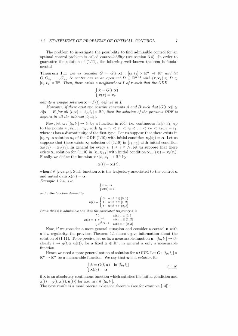
Now, let u : [t0, t1] → U be a function in KC, i.e. continuous in [t0, t1] upto the points τ1, τ2, . . . , τN , with t0 = τ0 < τ1 < τ2 < . . . < τN < τN+1 = t1,where u has a discontinuity of the first type. Let us suppose that there exists in[t0, τ1] a solution x0 of the ODE (1.10) with initial condition x0(t0) = α. Let ussuppose that there exists x1 solution of (1.10) in [τ1, τ2] with initial conditionx0(τ1) = x1(τ1). In general for every i, 1 ≤ i ≤ N, let us suppose that thereexists xi solution for (1.10) in [τi, τi+1] with initial condition xi−1(τi) = xi(τi).Finally we define the function x : [t0, t1]→ Rn by
x(t) = xi(t),
when t ∈ [τi, τi+1]. Such function x is the trajectory associated to the control uand initial data x(t0) = α.Example 1.2.4. Let
x = uxx(0) = 1
and u the function defined by
u(t) =
0 with t ∈ [0, 1)1 with t ∈ [1, 2]t with t ∈ (2, 3]
Prove that u is admissible and that the associated trajectory x is
x(t) =
1 with t ∈ [0, 1]et−1 with t ∈ (1, 2]
et2/2−1 with t ∈ (2, 3]
Now, if we consider a more general situation and consider a control u witha low regularity, the previous Theorem 1.1 doesn’t give information about thesolution of (1.11). To be precise, let us fix a measurable function u : [t0, t1]→ U :clearly t 7→ g(t,x,u(t)), for a fixed x ∈ Rn, in general is only a measurablefunction.
Hence we need a more general notion of solution for a ODE. Let G : [t0, t1]×Rn → Rn be a measurable function. We say that x is a solution for
x = G(t,x) in [t0, t1]x(t0) = α
(1.12)
if x is an absolutely continuous function which satisfies the initial condition andx(t) = g(t,x(t),u(t)) for a.e. in t ∈ [t0, t1].The next result is a more precise existence theorem (see for example [14]):

8 CHAPTER 1. INTRODUCTION TO OPTIMAL CONTROL
Theorem 1.2. Let us consider G = G(t,x) : [t0, t1]× Rn → Rn be such that
i. G is a measurable function;
ii. G is locally Lipschitz continuous with respect to x such that for everyR > 0 there exists a function lR : [t0, t1]→ [0,∞) in L1 with
|G(t,x)−G(t,x′)| ≤ lR(t)|x− x′|
for all x, x′ with |x| ≤ R, |x′| ≤ R and for a.e. t ∈ [t0, t1];
iii. G has at most a linear growth in the sense that there exist two positivefunctions A : [t0, t1] → [0,∞) and B : [t0, t1] → [0,∞) both in L1 suchthat
|G(t,x)| ≤ A(t)|x|+B(t)
for all x ∈ Rn and for a.e. t ∈ [t0, t1].
Then there exists a unique solution for (1.12).
Now we are in the position to give the precise notion of admissible controland associated trajectory :
Definition 1.1. Let g be a measurable function. We say that a measurablefunction u : [t0, t1] → U is an admissible control (or shortly control) for(1.11) if there exists a unique solution x of such ODE defined on [t0, t1]; we callsuch solution x trajectory associated to u. We denote by Ct0,α the set of theadmissible control for α at time t0.
In the next three chapters, in order to simplify the notation, we put C = Ct0,α.We say that a dynamics is linear if (1.10) is of the form
x(t) = A(t)x(t) +B(t)u(t), (1.13)
where A(t) is a square matrix of order n and B(t) is a matrix of order n × k :moreover the elements of such matrices are continuous function in [t0, t1]. Afundamental property of controllability of the linear dynamics is the following
Proposition 1.1. If the dynamics is linear and the trajectory has only a initialcondition (i.e. S = t1 × Rn), then every piecewise continuous function is anadmissible control for (1.11), i.e. exists the associated trajectory.
We remark that the previous proposition is false if we have a initial and a finalcondition on trajectory (see example 1.2.3).
The proof of the previous proposition is an easy application of the previoustheorems.
For every τ ∈ [t0, t1], we define the reachable set at time τ as the setR(τ, t0,α) ⊆ Rn of the points xτ such that there exists an admissible con-trol u and an associated trajectory x such that x(t0) = α and x(τ) = xτ .
If we consider the example 1.2.3, we have 36 6∈ R(2, 0, 1).

1.2. STATEMENT OF PROBLEMS OF OPTIMAL CONTROL 9
1.2.2 Optimal Control problems
Let us introduce the functional that we would like to optimize. Let us considerthe dynamics in (1.11), a function f : [t0,∞)×Rn+k → R, the so called runningcost (or running payoff) and a function ψ : [t0,∞)×Rn → R, the so called payoff .
Let U and S be control set and target respectively. Let us consider the setof admissible control C. We define J : C → R by
J(u) =
∫ T
t0
f(t,x(t),u(t)) dt+ ψ(T,x(T )),
where the function x is the (unique) trajectory associated to the control u thatsatisfies the initial and the final condition. This is the reason why J dependsonly on u. Hence our problem is
maxu∈C
J(u),
J(u) =
∫ T
t0
f(t,x,u) dt+ ψ(T,x(T ))
x = g(t,x,u) a.e. in [t0, T ]x(t0) = α(T,x(T )) ∈ SC = u : [t0, T ]→ U ⊆ Rk, u admissible
(1.14)
We say that u∗ ∈ C is an optimal control for (1.14) if
J(u) ≤ J(u∗), ∀u ∈ C.
The trajectory x∗ associated to the optimal control u∗, is called optimal trajec-tory.
In this problem and in more general problems, when f, g and ψ do notdepend directly on t, we say that the problem is autonomous.

10 CHAPTER 1. INTRODUCTION TO OPTIMAL CONTROL

Chapter 2
The simplest problem ofOC
In this chapter we are interested on the following problem
J(u) =
∫ t1
t0
f(t,x,u) dt
x = g(t,x,u)x(t0) = αmaxu∈C
J(u),
C = u : [t0, t1]→ U ⊆ Rk, u admissible
(2.1)
where t1 is fixed. The problem (2.1) is called the simplest problem of OptimalControl (in all that follows we shorten “Optimal Control” with OC).
2.1 The necessary condition of Pontryagin
Let us introduce the function
(λ0,λ) = (λ0, λ1, . . . , λn) : [t0, t1]→ Rn+1.
We call such function multiplier (or costate variable). We define the Hamiltonianfunction H : [t0, t1]× Rn × Rk × R× Rn → R by
H(t,x,u, λ0,λ) = λ0f(t,x,u) + λ · g(t,x,u).
The following result is fundamental:
Theorem 2.1 (Pontryagin). In the problem (2.1), let f and g be continuousfunctions with continuous derivatives with respect to x.Let u∗ be an optimal control and x∗ be the associated trajectory.Then there exists a multiplier (λ∗0,λ
∗), with
λ∗0 ≥ 0 constant,
λ∗ : [t0, t1]→ Rn continuous,
such that
11

12 CHAPTER 2. THE SIMPLEST PROBLEM OF OC
i) (nontriviality of the multiplier) (λ∗0,λ∗) 6= (0,0);
ii) (Pontryagin Maximum Principle, shortly PMP) for all t ∈ [t0, t1] we have
u∗(t) ∈ arg maxv∈U
H(t,x∗(t),v, λ∗0,λ∗(t)), i.e.
H(t,x∗(t),u∗(t), λ∗0,λ∗(t)) = max
v∈UH(t,x∗(t),v, λ∗0,λ
∗(t)); (2.2)
iii) (adjoint equation, shortly AE) we have
λ∗(t) = −∇xH(t,x∗(t),u∗(t), λ∗0,λ∗(t)), a.e. t ∈ [t0, t1]; (2.3)
iv) (transversality condition, shortly TC) λ∗(t1) = 0;
v) (normality) λ∗0 = 1.
If in addition the functions f and g are continuously differentiable in t, then forall t ∈ [t0, t1]
H(t,x∗(t),u∗(t), λ∗0,λ∗(t)) = H(t0,x
∗(t0),u∗(t0), λ∗0,λ∗(t0)) +
+
∫ t
t0
∂H
∂t(s,x∗(s),u∗(s), λ∗0,λ
∗(s)) ds (2.4)
The proof of this result is very long and difficult (see [22], [13], [10], [14], [28]):in section 2.1.1 we give a proof in a particular situation. Now let us list somecomments and definitions.
An admissible control u∗ that satisfies the conclusion of the theorem ofPontryagin is called extremal. We define (λ∗0,λ
∗) the associated multiplier tothe extremal u∗ as the function that satisfies the conclusion of the mentionedtheorem.
We mention that in the adjoint equation, since u∗ is a measurable function,the multiplier λ∗ is a solution of a ODE
λ = G(t,λ) in [t0, t1]
(here G is the second member of (2.3)), where G is a measurable function, affinein the λ variable, i.e. is a linear differential equation in λ with measurablecoefficients. This notion of solution is as in (1.12) and hence λ∗ is an absolutelycontinuous function.
We remark that we can rewrite the dynamics (1.10) as
x = ∇λH.
Normal and abnormal controls
It is clearly, in the previous theorem with the simplest problem of OC (2.1),that v. implies (λ∗0,λ
∗) 6= (0,0). If we consider a more generic problem (see forexample (1.14)), then it is not possible to guarantees λ∗0 = 1.
In general, there are two distinct possibilities for the constant λ∗0 :
a. if λ∗0 = 0, we say that u∗ is abnormal. Then the Hamiltonian H, for suchλ∗0, does not depend on f and the Pontryagin Maximum Principle is of nouse;
2.1. THE NECESSARY CONDITION OF PONTRYAGIN 13
b. if λ∗0 6= 0, we say that u∗ is normal: in this situation we may assume thatλ∗0 = 1.
Let us spend few words on this last assertion. Let u∗ be a normal extremalcontrol with x∗ and (λ∗0,λ
∗) associated trajectory and associated multiplierrespectively. It is an easy exercise to verify that (λ0, λ), defined by
λ0 = 1, λ =λ∗
λ∗0,
is again a multiplier associated to the normal control u∗. Hence, if u∗ is normal,we may assume that λ∗0 = 1. These arguments give that
Remark 2.1. In Theorem 2.1 we can replace λ∗0 ≥ 0 constant, with λ∗0 ∈ 0, 1.
The previous theorem 2.1 guarantees that
Remark 2.2. In the simplest optimal control problem (2.1) every extremal isnormal.
We will see in example 2.5.7 an abnormal optimal control.
On Maximum Principle with much more regularity
An important necessary condition of optimality in convex analysis1 implies
Remark 2.3. Let f and g be as in Theorem 2.1 with the additional assumptionthat they are differentiable with respect to the variable u. Let the control setU be convex and u∗ be optimal for (2.1). Since, for every fixed t, u∗(t) is amaximum for v 7→ H(t,x∗(t),v, λ∗0,λ
∗(t)), the PMP implies
∇uH(τ,x∗(t),u∗(t), λ∗0,λ∗(t)) · (v − u∗(t)) ≤ 0, (2.6)
for every v ∈ U, t ∈ [t0, t1].
When the control set coincides with Rk we have the following modification forthe PMP:
Remark 2.4. In the assumption of Remark 2.3, let U = Rk be the controlset for (2.1). In theorem 2.1 we can replace the PMP with the following newformulation
(PMP0) ∇uH(t,x∗(t),u∗(t), λ∗0,λ∗(t)) = 0, ∀ t ∈ [t0, t1],
1Theorem. Let U be a convex set in Rk and F : U → R be differentiable. If v∗ is a pointof maximum for F in U, then
∇F (v∗) · (v − v∗) ≤ 0, ∀v ∈ U. (2.5)
Proof: If v∗ is in the interior of U, then ∇F (v∗) = 0 and (2.5) is true. Let v∗ be onthe boundary of U : for all v ∈ U, let us consider the function f : [0, 1] → R defined byf(s) = F ((1− s)v∗ + sv). The formula of Mc Laurin gives f(s)− f(0) = f ′(0)s+ o(s), whereo(s)/s→ 0 for s→ 0+. Since v∗ is maximum we have
0 ≥ F ((1− s)v∗ + sv)− F (v∗)
= f(s)− f(0)
= f ′(0)s+ o(s)
= ∇F (v∗) · (v − v∗)s+ o(s).
Since s ≥ 0, (2.5) is true.

14 CHAPTER 2. THE SIMPLEST PROBLEM OF OC
On the Hamiltonian along the optimal path
In (2.4) let us consider the function
t 7→ h(t) := H(t,x∗(t),u∗(t), λ∗0,λ∗(t)) (2.7)
is a very regular function in [t0, t1] even though the control u∗ may be dis-continuous. More precisely and the very interesting propriety of (2.4) is thefollowing
Remark 2.5. In the problem (2.1), let f and g be continuous functions withcontinuous derivatives with respect to t and x. Let u∗ be a piecewise continuousoptimal control and x∗ be the associated trajectory. Then
• relation (2.4) is a consequence of the relations i)–v) of Theorem 2.1;
• the function h in (2.7) is absolutely continuous in [t0, t1] and
h(t) =∂H
∂t(t,x∗(t),u∗(t), λ∗0,λ
∗(t)).
This result is an easy consequence of the following lemma
Lemma 2.1. Let h = h(t,u) : [t0, t1] × Rk → R be a continuous functionwith continuous derivatives with respect to t. Let U ⊂ Rk be closed and letu∗ : [t0, t1]→ U be a left piecewise continuous function such that
u∗(t) ∈ arg maxv∈U
h(t,v), ∀t ∈ [t0, t1].
Let h : [t0, t1]→ R be a function such that
h(t) = maxv∈U
h(t,v) = h(t,u∗(t)) (2.8)
in [t0, t1]. Then h is absolutely continuous in [t0, t1] and
h(t) = h(t0) +
∫ t
t0
∂h
∂t(s,u∗(s)) ds, ∀t ∈ [t0, t1]. (2.9)
Proof. First let us prove that h is continuous. By the assumption h is leftpiecewise continuous and hence we have only to prove h is right continuous in[t0, t1], i.e. for every fixed t ∈ [t0, t1]
limτ→0+
h(t+ τ,u∗(t+ τ)) = h(t,u∗(t)) :
since h is continuous, the previous relation is equivalent to
limτ→0+
h(t,u∗(t+ τ)) = h(t,u∗(t)). (2.10)
Relation (2.8) implies that for a fixed t ∈ [t0, t1] and for every small τ we have
h(t,u∗(t+ τ)) ≤ h(t,u∗(t)), h(t+ τ,u∗(t)) ≤ h(t+ τ,u∗(t+ τ)).

2.1. THE NECESSARY CONDITION OF PONTRYAGIN 15
Hence considering the limits for τ → 0+ and using the continuity of h
limτ→0+
h(t,u∗(t+ τ)) ≤ limτ→0+
h(t,u∗(t)) = limτ→0+
h(t+ τ,u∗(t)) ≤
≤ limτ→0+
h(t+ τ,u∗(t+ τ)) = limτ→0+
h(t,u∗(t+ τ)).
Hence the previous inequalites are all equalities and (2.10) holds.Now let t be a point of continuity of u∗. The mean theorem implies that
there exist θ1 and θ2 in [0, 1] such that, for every small τ and using (2.8),
∂h
∂t(t+ θ1τ,u
∗(t))τ = h(t+ τ,u∗(t))− h(t,u∗(t))
≤ h(t+ τ,u∗(t+ τ))− h(t,u∗(t+ τ))
=∂h
∂t(t+ θ2τ,u
∗(t+ τ))τ
Since t is a point of continuity of u∗, dividing by τ and taking the limits asτ → 0 in the previous inequalities we have
∂h
∂t(t,u∗(t)) =
dh
dt(t,u∗(t)) =
dh
dt(t) = h′(t)
Since h has continuous derivative with respet to t, hence h has a piecewisecontinuous derivative: this implies that h has a derivative h′ a.e., such derivativeis Lebesgue integrable in [t0, t1], and clearly (2.9) holds.
Proof of Remark 2.5. We apply the previous lemma to the function
h(t,u) = H(t,x∗(t),u, λ∗0,λ∗(t)).
We have only to mention that if u∗ is not left piecewise continuous, then wehave to modify the control in a set of null measure.
An immediate consequence of (2.4) is the following important and usefulresult
Remark 2.6 (autonomous problems). If the problem is autonomous, i.e. f andg does not depend directly by t, and f, g are in C1, then (2.4) implies that
H(x∗(t),u∗(t), λ∗0,λ∗(t)) = constant in [t0, t1] (2.11)
2.1.1 The proof in a particular situation
In this section we consider a “simplest” optimal control problem (2.1) with twofundamental assumptions that simplify the proof of the theorem of Pontryagin:
a. we suppose that the control set is U = Rk.
b. We suppose that the set C = Ct0,α, i.e. the set of admissible controls, doesnot contain discontinuous function, is non empty and is open. We remarkthat with a linear dynamics, these assumptions on C are satisfied.

16 CHAPTER 2. THE SIMPLEST PROBLEM OF OC
In order to prove the mentioned theorem, we need a technical lemma:
Lemma 2.2. Let ϕ ∈ C([t0, t1]) and∫ t1
t0
ϕ(t)h(t) dt = 0 (2.12)
for every h ∈ C([t0, t1]). Then ϕ is identically zero on [t0, t1].
Proof. Let us suppose that ϕ(t′) 6= 0 for some point t′ ∈ [t0, t1] : we supposethat ϕ(t′) > 0 (if ϕ(t′) < 0 the proof is similar). Since ϕ is continuous, thereexists an interval [t′0, t
′1] ⊂ [t0, t1] containing t′ such that ϕ is positive.
Let us define the function h : [t0, t1]→ R as
h(t) = −(t− t′0)(t− t′1) 1[t′0,t′1]
(t),
where 1A is the indicator function on theset A. Hence
x
1
t
t0 tt’
h
t’0 t’1
∫ t1
t0
ϕ(t)h(t) dt = −∫ t′1
t′0
ϕ(t) (t− t′0)(t− t′1) dt > 0. (2.13)
On the other hand, (2.12) implies that
∫ t1
t0
ϕ(t)h(t) dt = 0. Hence (2.13) is
absurd and there does not exist such point t′.
Theorem 2.2. Let us consider the problem
J(u) =
∫ t1
t0
f(t,x,u) dt
x = g(t,x,u)x(t0) = αmaxu∈C
J(u)
C =u : [t0, t1]→ Rk, u ∈ C([t0, t1])
with f ∈ C1([t0, t1]×Rn+k) and g ∈ C1([t0, t1]×Rn+k); moreover let C be openand non empty.Let u∗ be the optimal control and x∗ be the optimal trajectory. Then there existsa multiplier λ∗ : [t0, t1]→ Rn continuous such that
(PMP0) ∇uH(t,x∗(t),u∗(t),λ∗(t)) = 0, ∀t ∈ [t0, t1] (2.14)
(AE) ∇xH(t,x∗(t),u∗(t),λ∗(t)) = −λ∗(t), ∀t ∈ [t0, t1] (2.15)
(TC) λ∗(t1) = 0, (2.16)
where H(t,x,u,λ) = f(t,x,u) + λ · g(t,x,u).
Proof. Let u∗ ∈ C be optimal control and x∗ its trajectory. Let us fix a
continuous function h = (h1, . . . , hk) : [t0, t1] → Rk. For every constant ε ∈ Rkwe define the function uε : [t0, t1]→ Rk by
uε = u∗ + (ε1h1, . . . , εkhk) = (u∗1 + ε1h1, . . . , u∗k + εkhk). (2.17)

2.1. THE NECESSARY CONDITION OF PONTRYAGIN 17
Since C is open, for every Let us show that uε ε with ‖ε‖ sufficiently small, uε isan admissible control.2 Hence, for such uε there exists the associated trajectory:we denote by xε : [t0, t1]→ Rn such trajectory associated3 to the control uε in(2.17). Clearly
u0(t) = u∗(t), x0(t) = x∗(t), xε(t0) = α. (2.18)
Now, recalling that h is fixed, we define the function Jh : Rk → R as
Jh(ε) =
∫ t1
t0
f(t,xε(t),uε(t)
)dt.
Since u∗ is optimal, Jh(0) ≥ Jh(ε), ∀ε; then ∇εJh(0) = 0. Let λ : [t0, t1]→ Rnbe a generic continuous function. Using the dynamics we have
Jh(ε) =
∫ t1
t0
[f(t,xε,uε
)+ λ ·
(g(t,xε,uε
)− xε
)]dt
=
∫ t1
t0
[H(t,xε,uε,λ
)− λ · xε
]dt
(by part) =
∫ t1
t0
[H(t,xε,uε,λ) + λ · xε
]dt−
(λ · xε
∣∣∣t1t0
For every i, with 1 ≤ i ≤ k, we have
∂Jh∂εi
=
∫ t1
t0
∇xH(t,xε,uε,λ) · ∇εixε(t) +
+∇uH(t,xε,uε,λ) · ∇εiuε(t) +
+λ · ∇εixε(t)
dt+
−λ(t1) · ∇εixε(t1) + λ(t0) · ∇εixε(t0).
2We remark that the assumption U = Rk is crucial. Suppose, for example, that U ⊂ R2 andlet us fix t ∈ [t0, t1]. If u∗(t) is an interior point of U, for every function h and for ε with modulosufficiently small, we have that uε(t) = (u∗1(t) + ε1h1(t), u∗2(t) + ε2h2(t)) ∈ U. If u∗(t) lies onthe boundary of U, is impossible to guarantee that, for every h, u(t) = u∗(t) + ε · h(t) ∈ U.
u*(t)
Uu* h(t)+ (t)e
u*(t)
U
The case u∗(t) in the interior of U ; the case u∗(t) on the boundary of U.
3For example, if n = k = 1 and the dynamics is linear we have, for every ε,xε(t) = a(t)xε(t) + b(t)[u∗(t) + εh(t)]xε(t0) = α
and hence xε(t) = e∫ tt0a(s) ds
(α+
∫ t
t0
b(s)[u∗(s) + εh(s)]e∫ st0a(w) dw
ds
).

18 CHAPTER 2. THE SIMPLEST PROBLEM OF OC
Note that (2.17) implies ∇εiuε(t) = (0, . . . , 0, hi, 0, . . . , 0), and (2.18) implies∇εixε(t0) = 0. Hence, by (2.18), we obtain
∂Jh∂εi
(0) =
∫ t1
t0
[∇xH(t,x∗,u∗,λ) + λ
]·(∇εixε(t)
∣∣∣∣ε=0
+
+∂H
∂ui(t,x∗,u∗,λ)hi(t)
dt+
−λ(t1) ·(∇εixε(t1)
∣∣∣∣ε=0
= 0. (2.19)
Now let us choose the function λ as the solution of the following ODE:λ = −∇xH(t,x∗,u∗,λ) for t ∈ [t0, t1]λ(t1) = 0
(2.20)
Since
∇xH(t,x∗,u∗,λ) = ∇xf(t,x∗,u∗) + λ · ∇xg(t,x∗,u∗),
this implies that the previous differential equation is linear (in λ). Hence, theassumption of the theorem implies that there exists a unique4 solution λ∗ ∈C([t0, t1]) of (2.20). Hence conditions (2.15) and (2.16) hold. For this choice ofthe function λ = λ∗, we have by (2.19)∫ t1
t0
∂H
∂ui(t,x∗,u∗,λ∗)hi dt = 0, (2.21)
for every i, with 1 ≤ i ≤ k, and h = (h1, . . . , hk) ∈ C([t0, t1]). Lemma 2.2 and(2.21) imply that ∂H
∂ui(t,x∗,u∗,λ∗) = 0 in [t0, t1] and hence (2.14).
2.2 Sufficient conditions
In order to study the problem (2.1), one of the main result about the sufficientconditions for a control to be optimal is due to Mangasarian (see [20]). Recallingthat in the simplest problem every extremal control is normal (see remark 2.2),we have:
Theorem 2.3 (Mangasarian). Let us consider the maximum problem (2.1) withf ∈ C1 and g ∈ C1. Let the control set U be convex. Let u∗ be a normal ex-tremal control, x∗ the associated trajectory and λ∗ = (λ∗1, . . . , λ
∗n) the associated
multiplier (as in theorem 2.1).Consider the Hamiltonian function H and let us suppose that
v) the function (x,u) 7→ H(t,x,u,λ∗) is, for every t ∈ [t0, t1], concave.
Then u∗ is optimal.
4We recall that for ODE of the first order with continuous coefficients holds the theorem1.1.

2.2. SUFFICIENT CONDITIONS 19
Proof. The assumptions of regularity and concavity on H imply5
H(t,x,u,λ∗) ≤ H(t,x∗,u∗,λ∗) +
+∇xH(t,x∗,u∗,λ∗) · (x− x∗) +
+∇uH(t,x∗,u∗,λ∗) · (u− u∗), (2.22)
for every admissible control u with associated trajectory x, and for every τ ∈[t0, t1]. The PMP implies, see (2.6), that
∇uH(τ,x∗(τ),u∗(τ),λ∗(τ)) · (u(τ)− u∗(τ)) ≤ 0. (2.23)
The adjoint equation ii), (2.22) and (2.23) imply
H(t,x,u,λ∗) ≤ H(t,x∗,u∗,λ∗)− λ∗ · (x− x∗). (2.24)
Since x and x∗ are trajectory associated to u and u∗ respectively, by (2.24) wehave
f(t,x,u) ≤ f(t,x∗,u∗) + λ∗ · (g(t,x∗,u∗)− g(t,x,u)) + λ∗ · (x∗ − x)
= f(t,x∗,u∗) + λ∗ · (x∗ − x) + λ∗ · (x∗ − x)
= f(t,x∗,u∗) +d
dt
(λ∗ · (x∗ − x)
). (2.25)
Hence, for every admissible control u with associated trajectory x, we have∫ t1
t0
f(t,x,u) dt ≤∫ t1
t0
f(t,x∗,u∗) dt+(λ∗ · (x∗ − x)
∣∣∣t1t0
(2.26)
=
∫ t1
t0
f(t,x∗,u∗) dt+
+λ∗(t1) ·(x∗(t1)− x(t1)
)− λ∗(t0) ·
(x∗(t0)− x(t0)
);
since x∗(t0) = x(t0) = α and the transversality condition iii) are satisfied, weobtain that u∗ is optimal.
In order to apply such theorem, it is easy to prove the next note
Remark 2.7. If we replace the assumption v) of theorem 2.3 with one of thefollowing assumptions
v’) for every t ∈ [t0, t1], let f and g be concave in the variables x and u, andlet us suppose λ∗(t) ≥ 0, (i.e. for every i, 1 ≤ i ≤ n, λ∗i (t) ≥ 0);
v”) let the dynamics of problem (2.1) be linear and, for every t ∈ [t0, t1], let fbe concave in the variables x and u;
then u∗ is optimal.
5We recall that if F is a differentiable function on a convex set C ⊆ Rn, then F is concavein C if and only if, for every v, v′ ∈ C, we have F (v) ≤ F (v′) +∇F (v′) · (v − v′).
20 CHAPTER 2. THE SIMPLEST PROBLEM OF OC
A further sufficient condition is due to Arrow: we are interested in a partic-ular situation of the problem (2.1), more precisely
maxu∈C
∫ t1
t0
f(t,x,u) dt
x = g(t,x,u)x(t0) = αC = u : [t0, t1]→ U, u admissible
(2.27)
with U ⊂ Rk (note that we do not require convexity of the control set). Letus suppose that it is possible to define the maximized Hamiltonian functionH0 : [t0, t1]× Rn × Rn → R by
H0(t,x,λ) = maxu∈U
H(t,x,u,λ), (2.28)
where, as usual, H(t,x,u,λ) = f(t,x,u)+λ ·g(t,x,u) is the Hamiltonian. Wehave the following result by Arrow (see [2], [9] section 8.3, [17] part II section15, theorem 2.5 in [26]):
Theorem 2.4 (Arrow). Let us consider the maximum problem (2.27) with f ∈C1 and g ∈ C1. Let u∗ be a normal extremal control, x∗ be the associatedtrajectory and λ∗ be the associated multiplier.Let us suppose that the maximized Hamiltonian function H0 exists and, forevery t ∈ [t0, t1]× Rn, the function
x 7→ H0(t,x,λ∗)
is concave. Then u∗ is optimal.
Proof. Let us consider t fixed in [t0, t1] (and hence we have x∗ = x∗(t), u∗ =u∗(t), . . .). Our aim is to arrive to prove relation (2.24) with our new assump-tions. First of all we note that the definitions of H0 imply
H0(t,x∗,λ∗) = H(t,x∗,u∗,λ∗)
and H(t,x,u,λ∗) ≤ H0(t,x,λ∗) for every x, u. These relations give
H(t,x,u,λ∗)−H(t,x∗,u∗,λ∗) ≤ H0(t,x,λ∗)−H0(t,x∗,λ∗). (2.29)
Since the function g : Rn → R, defined by g(x) = H0(t,x,λ∗), is concave thenthere exists a supergradient6 a in the point x∗, i.e.
H0(t,x,λ∗) ≤ H0(t,x∗,λ∗) + a · (x− x∗), ∀x ∈ Rn. (2.30)
6We recall that (see [24]) if we consider a function g : Rn → R, we say that a ∈ Rn is asupergradient (respectively subgradient) in the point x0 if
g(x) ≤ g(x0) + a · (x− x0) ∀x ∈ Rn (respectivelly g(x) ≥ g(x0) + a · (x− x0) ).
A fundamental result in convex analysis is the following
Theorem 2.5 (Rockafellar). Let g : Rn → R a concave (convex) function. Then, for everyx0 ∈ Rn, the set of the supergradients (subgradients) in x0 is non empty.
2.3. FIRST GENERALIZATIONS 21
Clearly from (2.29) and (2.30) we have
H(t,x,u,λ∗)−H(t,x∗,u∗,λ∗) ≤ a · (x− x∗). (2.31)
In particular, choosing u = u∗, we have
H(t,x,u∗,λ∗)−H(t,x∗,u∗,λ∗) ≤ a · (x− x∗). (2.32)
Now let us define the function G : Rn → R by
G(x) = H(t,x,u∗,λ∗)−H(t,x∗,u∗,λ∗)− a · (x− x∗).
Clearly, by (2.32), G has a maximum in the point x∗: moreover it is easy to seethat G is differentiable. We obtain
0 = ∇G(x∗) = ∇xH(t,x∗,u∗,λ∗)− a.
Now, the adjoint equation and (2.31) give
H(t,x,u,λ∗) ≤ H(t,x∗,u∗,λ∗)− λ∗ · (x− x∗).
Note that this last relation coincides with (2.24): at this point, using the samearguments of the second part of the proof of Theorem 2.3, we are able to concludethe proof.
2.3 First generalizations
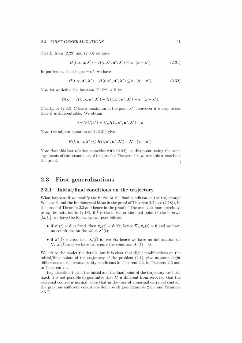
2.3.1 Initial/final conditions on the trajectory
What happens if we modify the initial or the final condition on the trajectory?We have found the fundamental ideas in the proof of Theorem 2.2 (see (2.18)), inthe proof of Theorem 2.3 and hence in the proof of Theorem 2.4: more precisely,using the notation in (2.18), if t is the initial or the final point of the interval[t0, t1], we have the following two possibilities:
• if x∗(t) = α is fixed, then xε(t) = α ∀ε; hence ∇εixε(t) = 0 and we haveno conditions on the value λ∗(t);
• if x∗(t) is free, then xε(t) is free ∀ε; hence we have no information on∇εixε(t) and we have to require the condition λ∗(t) = 0.
We left to the reader the details, but it is clear that slight modifications on theinitial/final points of the trajectory of the problem (2.1), give us some slightdifferences on the transversality conditions in Theorem 2.2, in Theorem 2.3 andin Theorem 2.4.
Pay attention that if the initial and the final point of the trajectory are bothfixed, it is not possible to guarantee that λ∗0 is different from zero, i.e. that theextremal control is normal: note that in the case of abnormal extremal control,the previous sufficient conditions don’t work (see Example 2.5.3 and Example2.5.7).

22 CHAPTER 2. THE SIMPLEST PROBLEM OF OC
2.3.2 On minimum problems
Let us consider the problem (2.1) where we replace the maximum with a mini-mum problem. Since
min
∫ t1
t0
f(t,x,u) dt = −max
∫ t1
t0
−f(t,x,u) dt,
clearly it is possible to solve a min problem passing to a max problem with someminus.
Basically, a more direct approach consists in replace some “words” in all theprevious pages as follows
max → minconcave function → convex function.
In particular in (2.2) we obtain the Pontryagin Minimum Principle.
2.4 The case of Calculus of Variation
A very particular situation appears when the dynamics (1.10) is of the typex = g(t,x,u) = u (and hence k = n) and the control set U is Rn. Clearly it ispossible to rewrite the problem7 (2.1) as
J(x) =
∫ t1
t0
f(t,x, x) dt
x(t0) = αmax
x∈KC1J(x)
(2.33)
This problems are called Calculus of Variation problems (shortly CoV). Clearlyin this problem the control does not appear. We say that x∗ ∈ KC1 is optimalfor (2.33) if
J(x) ≤ J(x∗), ∀x ∈ KC1, x(t0) = α.
In this section, we will show that the theorem of Euler of Calculus of Vari-ation is an easy consequence of the theorem of Pontryagin of Optimal Control.Hence we are interested in the problem max
x∈C1
∫ t1
t0
f(t,x, x) dt
x(t0) = α
(2.34)
with α ∈ Rn fixed. We remark that here x is in C1. We have the followingfundamental result
Theorem 2.6 (Euler). Let us consider the problem (2.34) with f ∈ C1.Let x∗ be optimal. Then, for all t ∈ [t0, t1], we have
d
dt
(∇xf(t,x∗(t), x∗(t))
)= ∇xf(t,x∗(t), x∗(t)). (2.35)
7We remark that in general in a Calculus of Variation problem one assume that x ∈ KC1;in this note we are not interested in this general situation and we will assume that x ∈ C1.

2.4. THE CASE OF CALCULUS OF VARIATION 23
In calculus of variation the equation (2.35) is called Euler equation (shortlyEU); a function that satisfies EU is called extremal. Let us prove this result. Ifwe consider a new variable u = x, we rewrite problem (2.34) as
maxu∈C
∫ t1
t0
f(t,x,u) dt
x = ux(t0) = α
Theorem 2.2 guarantees that, for the Hamiltonian H(t,x,u,λ) = f(t,x,u) +λ · u, we have
∇uH(t,x∗,u∗) = 0 ⇒ ∇uf + λ∗ = 0 (2.36)
∇xH(t,x∗,u∗) = −λ∗⇒ ∇xf = −λ
∗(2.37)
If we consider a derivative with respect to the time in (2.36) and using (2.36)we have
d
dt(∇uf) = −λ
∗= ∇xf ;
taking into account x = u, we obtain (2.35). Moreover, we are able to find thetransversality condition of Calculus of Variation: (2.16) and (2.36), imply
∇xf(t1,x∗(t1), x∗(t1)) = 0.
As in subsection 2.3.1 we obtain
Remark 2.8. Consider the theorem 2.6, its assumptions and let us modifyslightly the conditions on the initial and the final points of x. We have thefollowing transversality conditions:
if x∗(ti) ∈ Rn, i.e. x∗(ti) is free ⇒ ∇xf(ti,x∗(ti), x
∗(ti)) = 0,
where ti is the initial or the final point of the interval [t0, t1].
An useful remark, in some situation, is that if f does not depend on x, i.e.f = f(t, x), then the equation of Euler (2.35) is
∇xf(t, x∗) = c,
where c ∈ R is a constant. Moreover, the following remark is not so obvious:
Remark 2.9. If f = f(x, x) does not depend directly on t, then the equation ofEuler (2.35) is
f(x∗, x∗)− x∗ · ∇xf(x∗, x∗) = c, (2.38)
where c ∈ R is a constant.
Proof. Clearly
d
dtf = x · ∇xf + x · ∇xf,
d
dt(x · ∇xf) = x · ∇xf + x · d
dt(∇xf).

24 CHAPTER 2. THE SIMPLEST PROBLEM OF OC
Now let us suppose that x∗ satisfies condition the Euler condition (2.35): hence,using the previous two equalities we obtain
0 = x∗ ·(
d
dt
(∇xf(x∗, x∗)
)−∇xf(x∗, x∗)
)=
d
dt
(x∗ · ∇xf(x∗, x∗)
)− d
dt
(f(x∗, x∗)
)=
d
dt
(x∗ · ∇xf(x∗, x∗)− f(x∗, x∗)
).
Hence we obtain (2.38).
If we are interested to find sufficient condition of optimality for the problem(2.34), since the dynamics is linear, remark 2.7 implies
Remark 2.10. Let us consider an extremal x∗ for the problem (2.34) in theassumption of theorem of Euler. Suppose that x∗ satisfies the transversalityconditions. If, for every t ∈ [t0, t1], the function f is concave on the variable xand x, then x∗ is optimal.
2.5 Examples and applications
Example 2.5.1. Consider8 max
∫ 1
0(x− u2) dt
x = ux(0) = 2
1st method: Clearly the Hamiltonian is H = x− u2 + λu (note that the extremal is certainlynormal) and theorem 2.2 implies
∂H
∂u= 0 ⇒ −2u∗ + λ∗ = 0 (2.39)
∂H
∂x= −λ∗ ⇒ 1 = −λ∗ (2.40)
∂H
∂λ= x∗ ⇒ x∗ = u∗ (2.41)
λ∗(1) = 0 (2.42)
Equations (2.40) and (2.42) give λ∗ = 1− t; consequently, by (2.39) we have u∗ = (1− t)/2;since the dynamics is linear, sure the previous control u∗ is admissible (see Proposition 1.1).Finally, since the HamiltonianH is concave in x and u, the sufficient conditions of Mangasarianin theorem 2.3 guarantees that the extremal u∗ is optimal.
If we are interested to find the optimal trajectory, the initial condition and (2.41) givex∗ = (2t− t2)/4 + 2.
2nd method: The problem is, clearly, of calculus of variations, i.e.max
∫ 1
0(x− x2) dt
x(0) = 2
The necessary condition of Euler (2.35) and the transversality condition give
dfx
dt(t, x∗, x∗) = fx(t, x∗, x∗) ⇒ −2x∗ = 1
⇒ x∗(t) = −1
4t2 + at+ b, ∀a, b ∈ R
fx(1, x∗(1), x∗(1)) = 0 ⇒ −2x∗(1) = 0
8In the example 5.5.1 we solve the same problem with the dynamics programming.

2.5. EXAMPLES AND APPLICATIONS 25
An easy calculation, using the initial condition x(0) = 2, implies x∗(t) = −t2/4 + t/2 + 2.Since the function (x, x) 7→ (x− x2) is concave, then x∗ is really the maximum of the problem.
Example 2.5.2. Consider9 max
∫ 2
0(2x− 4u) dt
x = x+ ux(0) = 50 ≤ u ≤ 2
Let us consider the Hamiltonian H = 2x− 4u+ λ(x+ u) (note that the extremal is certainlynormal). The theorem of Pontryagin gives
H(t, x∗, u∗, λ∗) = maxv∈[0,2]
H(t, x∗, v, λ∗) ⇒
⇒ 2x∗ − 4u∗ + λ∗(x∗ + u∗) = maxv∈[0,2]
(2x∗ − 4v + λ∗(x∗ + v)) (2.43)
∂H
∂x= −λ∗ ⇒ 2 + λ∗ = −λ∗ (2.44)
∂H
∂λ= x∗ ⇒ x∗ = x∗ + u∗ (2.45)
λ∗(2) = 0 (2.46)
From (2.43) we have, for every t ∈ [0, 2],
u∗(t)(λ∗(t)− 4) = maxv∈[0,2]
(v(λ∗(t)− 4))
and hence
u∗(t) =
2 for λ∗(t)− 4 > 0,0 for λ∗(t)− 4 < 0,? for λ∗(t)− 4 = 0.
(2.47)
(2.44) implies λ∗(t) = ae−t − 2, ∀a ∈ R : using (2.46) we obtain
λ∗(t) = 2(e2−t − 1). (2.48)
Since λ∗(t) > 4 if and only if t ∈ [0, 2− log 3), the extremal control is
u∗(t) =
2 for 0 ≤ t ≤ 2− log 3,0 for 2− log 3 < t ≤ 2.
(2.49)
We remark that the value of the function u∗ in t = 2− log 3 is irrelevant. Since the dynamicsis linear, the previous control u∗ is admissible (see Proposition 1.1). Finally, the Hamiltonianfunction H is concave in (x, u) for every λ fixed, and hence u∗ is optimal.
If we are interested to find the optimal trajectory, the relations (2.45) and (2.49), and theinitial condition give us to solve the ODE
x∗ = x∗ + 2 in [0, 2− log 3)x(0) = 5
(2.50)
The solution is x∗(t) = 7et − 2. Taking into account that the trajectory is a continuousfunction, by (2.50) we have x∗(2 − log 3) = 7e2−log 3 − 2 = 7e2/3 − 2. Hence the relations(2.45) and (2.49) give us to solve the ODE
x∗ = x∗ in [2− log 3, 2]x(2− log 3) = 7e2/3− 2
We obtain
x∗(t) =
7et − 2 for 0 ≤ t ≤ 2− log 3,(7e2 − 6)et−2 for 2− log 3 < t ≤ 2.
(2.51)
t0
u
2-log 3 2
2
t0
x
2-log 3 2
5
9In the example 5.5.3 we solve the same problem with the dynamics programming.

26 CHAPTER 2. THE SIMPLEST PROBLEM OF OC
We note that an easy computation gives H(t, x∗(t), u∗(t), λ∗(t)) = 14e2 − 12 for all t ∈ [0, 2].
4
Example 2.5.3. Find the optimal tern formax
∫ 4
03xdt
x = x+ ux(0) = 0x(4) = 3e4/20 ≤ u ≤ 2
Let us consider the Hamiltonian H = 3x + λ(x + u); it is not possible to guarantee that theextremal is normal, but we try to put λ0 = 1 since this situation is more simple; if we will notfound an extremal (more precisely a normal extremal), then we will pass to the more generalHamiltonian H = 3λ0x+ λ(x+ u) (and in this situation certainly the extremal there exists).The theorem of Pontryagin gives
H(t, x∗, u∗, λ∗) = maxv∈[0,2]
H(t, x∗, v, λ∗) ⇒ λ∗u∗ = maxv∈[0,2]
λ∗v
⇒ u∗(t) =
2 for λ∗(t) > 0,0 for λ∗(t) < 0,? for λ∗(t) = 0.
(2.52)
∂H
∂x= −λ∗ ⇒ 3 + λ∗ = −λ∗ ⇒ λ∗(t) = ae−t − 3, ∀a ∈ R (2.53)
∂H
∂λ= x∗ ⇒ x∗ = x∗ + u∗ (2.54)
Note that we have to maximize the area of the function t 7→ 3x(t) and that x(t) ≥ 0 sincex(0) = 0 and x = u + x ≥ x ≥ 0. In order to maximize the area, it is reasonable that thefunction x is increasing in an interval of the type [0, α) : hence it is reasonable to suppose thatthere exists a positive constant α such that λ∗(t) > 0 for t ∈ [0, α). In this case, (2.52) givesu∗ = 2. Hence we have to solve the ODE
x∗ = x∗ + 2 in [0, α)x(0) = 0
(2.55)
The solution is x∗(t) = 2(et− 1). We note that for such function we have x∗(4) = 2(e4− 1) >3e4/2; hence it is not possible that α ≥ 4 : we suppose that λ∗(t) < 0 for t ∈ (α, 4]. Takinginto account the final condition on the trajectory, we have to solve the ODE
x∗ = x∗ in (α, 4]x(4) = 3e4/2
(2.56)
The solution is x∗(t) = 3et/2. We do not know the point α, but certainly the trajectory iscontinuous, i.e.
limt→α−
x∗(t) = limt→α+
x∗(t) ⇒ limt→α−
2(et − 1) = limt→α+
3et/2
that implies α = ln 4. Moreover, since the multiplier is continuous, we are in the positionto find the constant a in (2.53): more precisely λ∗(t) = 0 for t = ln 4, implies a = 12, i.e.λ∗(t) = 12e−t − 3. Note that the previous assumptions λ∗ > 0 in [0, ln 4) and λ∗ < 0 in(ln 4, 4] are verified. These calculations give that u∗ is admissible.
Finally, the dynamics and the running cost is linear (in x and u) and hence the sufficientcondition are satisfied. The optimal tern is
u∗(t) =
2 for t ∈ [0, ln 4),0 for t ∈ [ln 4, 4]
(2.57)
x∗(t) =
2(et − 1) for t ∈ [0, ln 4),3et/2 for t ∈ [ln 4, 4]
λ∗(t) = 12e−t − 3. We note that an easy computation gives H(t, x∗(t), u∗(t), λ∗(t)) = 18 for
all t ∈ [0, 4]. 4

2.5. EXAMPLES AND APPLICATIONS 27
Example 2.5.4. min
∫ e
1(3x+ tx2) dt
x(1) = 1x(e) = 1
It is a calculus of variation problem. Since f = 3x+ tx2 does not depend on x, the necessarycondition of Euler implies
3 + 2tx = c,
where c is a constant. Hence x(t) = a/t, ∀a ∈ R, implies the solution x(t) = a ln t+b, ∀a, b ∈ R.Using the initial and the final conditions we obtain the extremal x∗(t) = 1. Since f is convexin x and x, the extremal is the minimum of the problem.
4
Example 2.5.5. min
∫ √2
0(x2 − xx+ 2x2) dt
x(0) = 1
It is a calculus of variation problem; the necessary condition of Euler (2.35) gives
d
dtfx = fx ⇒ 4x− x = 2x− x
⇒ 2x− x = 0 ⇒ x∗(t) = aet/√2 + be−t/
√2,
for every a, b ∈ R. Hence the initial condition x(0) = 1 gives b = 1 − a. Since there does notexist a final condition on the trajectory, we have to satisfy the transversality condition, i.e.
fx(t1, x∗(t1), x∗(t1)) = 0 ⇒ 4x∗(
√2)− x∗(
√2)− = 0
⇒ ae+1− ae− 4
[ae√
2−
1− ae√
2
]= 0
Hence
x∗(t) =(4 +
√2)et/
√2 + (4e2 − e2
√2)e−t/
√2
4 +√
2 + 4e2 − e2√
2.
The function f(t, x, x) = x2 − xx + 2x2 is convex in the variable x and x, since its hessianmatrix with respect (x, x)
d2f =
(2 −1
−1 4
),
is positive definite. Hence x∗ is minimum. 4
Example 2.5.6. min
∫ 2
1(t2x2 + 2x2) dt
x(2) = 17
It is a calculus of variation problem; the necessary condition of Euler (2.35) gives
d
dtfx = fx ⇒ t2x+ 2tx− 2x = 0.
The homogeneity suggests to set t = es and y(s) = x(es) : considering the derivative of thislast expression with respect to s we obtain
y′(s) = x(es)es = tx(t) and y′′(s) = x(es)e2s + x(es)es = t2x(t) + tx(t).
Hence the Euler equation now isy′′ + y′ − 2y = 0.
This implies y(s) = aes + be−2s, with a, b constants. The relation t = es gives
x∗(t) = at+b
t2.
Note that x∗(s) = a − 2bt3. The final condition x∗(2) = 17 and the transversality condition
fx(1, x∗(1), x∗(1)) = 0 give, respectively,
17 = 2a+b
4and 2(a− 2b) = 0.

28 CHAPTER 2. THE SIMPLEST PROBLEM OF OC
Hence x∗(t) = 8t + 4t2
is the unique extremal function which satisfies the transversality
condition and the final condition. The function f(t, x, x) = t2x2 + 2x2 is convex in the
variable x and x and x∗ is clearly the minimum. 4
The following example gives an abnormal control.
Example 2.5.7. Let us consider max
∫ 1
0u dt
x = (u− u2)2
x(0) = 0x(1) = 00 ≤ u ≤ 2
We prove that u∗ = 1 is an abnormal extremal and optimal. Clearly H = λ0u+ λ(u− u2)2;the PMP and the adjoint equation give
u∗(t) ∈ arg maxv∈[0,2]
[λ∗0v + λ∗(t)(v − v2)2], λ = 0.
This implies that λ∗ = k, with k constant; hence u∗ is constant. If we define the functionφ(v) = λ∗0v + k(v − v2)2, the study of the sign of φ′ depends on λ∗0 and k and it is not easyto obtain some information on the max.
However, we note that the initial and the final conditions on the trajectory and the factthat x = (u − u2)2 ≥ 0, implies that x = 0 a.e.; hence if a control u is admissible, then wehave u(t) ∈ 0, 1 a.e. This implies that considering u∗ = 1, for every admissible control u,∫ 1
0u∗(t) dt =
∫ 1
01 dt ≥
∫ 1
0u(t) dt;
hence u∗ = 1 is maximum.Now, since u∗ is optimal, then it satisfies the PMP: hence we have
1 = u∗(t) ∈ arg maxv∈[0,2]
φ(v).
Since we realize the previous max in an interior point of the interval [0, 2], we necessarily have
φ′(1) = 0: an easy calculation gives λ∗0 = 0. This proves that u∗ is abnormal. 4
2.5.1 The curve of minimal length
We have to solve the calculus of variation problem (1.1). Since the functionf(t, x, x) =
√1 + x2 does not depend on x, the necessary condition of Euler
(2.35) gives
fx = a ⇒ x√1 + x2
= a
⇒ x = c ⇒ x∗(t) = ct+ d,
with a, b, c ∈ R constants. The conditions x(0) = 0 and x(1) = b imply x∗(t) =bt. The function f is constant and hence convex in x and it is convex in x since∂2f∂x2 = (1 + x2)−3/2 > 0. This proves that the line x∗ is the solution of theproblem.
2.5.2 A problem of business strategy I
We solve10 the model presented in the example 1.1.2, formulated with (1.3).
10In subsection 5.5.1 we solve the same problem with the Dynamic Programming approach.

2.5. EXAMPLES AND APPLICATIONS 29
We consider the Hamiltonian H = (1− u)x+ λxu : the theorem of Pontryaginimplies that
H(t, x∗, u∗, λ∗) = maxv∈[0,1]
H(t, x∗, v, λ∗)
⇒ (1− u∗)x∗ + λ∗x∗u∗ = maxv∈[0,1]
[(1− v)x∗ + λ∗x∗v]
⇒ u∗x∗(λ∗ − 1) = maxv∈[0,1]
[vx∗(λ∗ − 1)] (2.58)
∂H
∂x= −λ∗ ⇒ 1− u∗ + λ∗u∗ = −λ∗ (2.59)
∂H
∂λ= x∗ ⇒ x∗ = x∗u∗ (2.60)
λ∗(T ) = 0 (2.61)
Since x∗ is continuous, x∗(0) = α > 0 and u∗ ≥ 0, from (2.60) we obtain
x∗ = x∗u∗ ≥ 0, (2.62)
in [0, T ]. Hence x∗(t) ≥ α for all t ∈ [0, T ]. Relation (2.58) becomes
u∗(λ∗ − 1) = maxv∈[0,1]
v(λ∗ − 1).
Hence
u∗(t) =
1 if λ∗(t)− 1 > 0,0 if λ∗(t)− 1 < 0,? if λ∗(t)− 1 = 0.
(2.63)
Since the multiplier is a continuous function that satisfies (2.61), there existsτ ′ ∈ [0, T ) such that
λ∗(t) < 1, ∀t ∈ [τ ′, T ] (2.64)
Using (2.63) and (2.64), we have to solve the ODEλ∗ = −1 in [τ ′, T ]λ∗(T ) = 0
that impliesλ∗(t) = T − t, ∀t ∈ [τ ′, T ]. (2.65)
Clearly, we have two cases: T ≤ 1 (case A) and T > 1 (case B).
l
t0T
1
1
l*
l
t0T
1
T-1
l*
??
The case T ≤ 1 and the case T > 1.
Case A: T ≤ 1.In this situation, we obtain τ ′ = 0 and hence u∗ = 0 and x∗ = α in [0, T ].

30 CHAPTER 2. THE SIMPLEST PROBLEM OF OC
u
t0T 1
u*
x
t0T 1
a
*x
l
t0T
1
1
l*
From an economic point of view, if the time horizon is short the optimal strategyis to sell all our production without any investment. Note that the strategy u∗
that we have found is an extremal: in order to guarantee the sufficient conditionsfor such extremal we refer the reader to the case B.Case B: T ≥ 1.In this situation, taking into account (2.63), we have τ ′ = T − 1. Hence
λ∗(T − 1) = 1. (2.66)
First of all, if there exists an interval I ⊂ [0, T − 1) such that λ∗(t) < 1, thenu∗ = 0 and the (2.59) is λ∗ = −1 : this is impossible since λ∗(T − 1) = 1.Secondly, if there exists an interval I ⊂ [0, T − 1) such that λ∗(t) = 1, thenλ∗ = 0 and the (2.59) is 1 = 0 : this is impossible.Let us suppose that there exists an interval I = [τ ′′, T − 1) ⊂ [0, T − 1) suchthat λ∗(t) > 1 : using (2.63), we have to solve the ODE
λ∗ + λ∗ = 0 in [τ ′′, T − 1]λ∗(T − 1) = 1
that impliesλ∗(t) = eT−t−1, for t ∈ [0, T − 1].
We remark the choice τ ′′ = 0 is consistent with all the necessary conditions.Hence (2.63) gives
u∗(t) =
1 for 0 ≤ t ≤ T − 1,0 for T − 1 < t ≤ T (2.67)
The continuity of the function x∗, the initial condition x(0) = α and the dy-namics imply
x∗ = x∗ in [0, T − 1]x∗(0) = α
that implies x∗(t) = αet; hencex∗ = 0 in [T − 1, T ]x∗(T − 1) = αeT−1
that implies x∗(t) = αeT−1. Consequently
x∗(t) =
αet for 0 ≤ t ≤ T − 1,αeT−1 for T − 1 < t ≤ T
Recalling that
λ∗(t) =
eT−t−1 for 0 ≤ t ≤ T − 1,T − t for T − 1 < t ≤ T
we have

2.5. EXAMPLES AND APPLICATIONS 31
u
u*
t0
T
1
T-1
x
x
t0
TT-1
*
a
l
t0
T
1
T-1
l*
In an economic situation where the choice of business strategy can be carriedout in a medium or long term, the optimal strategy is to direct all output toincrease production and then sell everything to make profit in the last period.
We remark, that we have to prove some sufficient conditions for the tern(x∗, u∗, λ∗) in order to guarantee that u∗ is really the optimal strategy. Aneasy computation shows that the Hamiltonian is not concave. We study themaximized Hamiltonian (2.28): taking into account that x(t) ≥ α > 0 weobtain
H0(t, x, λ) = maxv∈[0,1]
[(1− v)x+ λxv] = x+ x maxv∈[0,1]
[(λ− 1)v]
In order to apply theorem 2.4, using the expression of λ∗ we obtain
H0(t, x, λ∗(t)) =
eT−t−1x if t ∈ [0, T − 1)x if t ∈ [T − 1, T ]
Note that, for every fixed t the function x 7→ H0(t, x, λ∗(t)) is concave withrespect to x: the sufficient condition of Arrow holds. We note that an easycomputation gives H(t, x∗(t), u∗(t), λ∗(t)) = αeT−1 for all t ∈ [0, T ].
2.5.3 A two-sector model
This model has some similarities with the previous one and it is proposed in[26].
Consider an economy consisting of two sectors where sector no. 1 producesinvestment goods, sector no. 2 produces consumption goods. Let xi(t) theproduction in sector no. i per unit of time, i = 1, 2, and let u(t) be the proportionof investments allocated to sector no. 1. We assume that x1 = αux1 andx2 = α(1−u)x1 where α is a positive constant. Hence, the increase in productionper unit of time in each sector is assumed to be proportional to investmentallocated to the sector. By definition, 0 ≤ u(t) ≤ 1, and if the planning periodstarts at t = 0, x1(0) and x2(0) are historically given. In this situation a numberof optimal control problems could be investigated. Let us, in particular, considerthe problem of maximizing the total consumption in a given planning period[0,T ]. Our precise problem is as follows:
maxu∈C
∫ T
0
x2 dt
x1 = αux1x2 = α(1− u)x1x1(0) = a1x2(0) = a2C = u : [0, T ]→ [0, 1] ⊂ R, u admissible

32 CHAPTER 2. THE SIMPLEST PROBLEM OF OC
where α, a1, a2 and T are positive and fixed. We study the case T > 2α .
We consider the Hamiltonian H = x2 + λ1ux1 + λ2(1 − u)x1; the theorem ofPontryagin implies that
u∗ ∈ arg maxv∈[0,1]
H(t, x∗, v, λ∗) = arg maxv∈[0,1]
[x∗2 + λ∗1vx∗1 + λ∗2(1− v)x∗1]
⇒ u∗ ∈ arg maxv∈[0,1]
(λ∗1 − λ∗2)vx∗1 (2.68)
∂H
∂x1= −λ∗1 ⇒ −λ∗1u∗α− λ∗2α(1− u∗) = λ∗1 (2.69)
∂H
∂x2= −λ∗2 ⇒ −1 = λ∗2 (2.70)
λ∗1(T ) = 0 (2.71)
λ∗2(T ) = 0 (2.72)
Clearly (2.70) and (2.72) give us λ∗2(t) = T − t. Moreover (2.71) and (2.72) inequation (2.69) give λ∗1(T ) = 0. We note that
λ∗1(T ) = λ∗2(T ) = 0, λ∗1(T ) = 0, λ∗2(T ) = −1
and the continuity of the multiplier (λ∗1, λ∗2) implies that there exists τ < T such
thatT − t = λ∗2(t) > λ∗1(t), ∀t ∈ (τ, T ). (2.73)
Since x∗1 is continuous, using the dynamics x1 = αux1 x∗1(0) = a1 > 0 and
u∗ ≥ 0, we have x1(t) ≥ 0 and hence x∗1(t) ≥ a1 > 0; from (2.68) we obtain
u∗(t) ∈ arg maxv∈[0,1]
(λ∗1(t)− T + t)v =
1 if λ∗1(t) > T − t? if λ∗1(t) = T − t0 if λ∗1(t) < T − t
(2.74)
Hence (2.73) and (2.74) imply that, in (τ, T ], we have u∗(t) = 0. Now (2.69)gives, taking into account (2.72),
λ∗1 = −λ∗2α ⇒ λ∗1(t) =α
2(t− T )2, ∀t ∈ (τ, T ].
An easy computation shows that the relation in (2.73) holds for τ = T − 2α .
Hence let us suppose that there exists τ ′ < T − 2α such that
T − t = λ∗2(t) < λ∗1(t), ∀t ∈ (τ ′, T − 2/α). (2.75)
By (2.74) we obtain, in (τ ′, T − 2/α), that u∗(t) = 1. Now (2.69) gives, takinginto account the continuity of λ∗2 in the point T − 2/α,
λ∗1 = −λ∗1α ⇒ λ∗1(t) =2
αe−α(t−T+2/α), ∀t ∈ (τ ′, T − 2/α].
Since λ∗1(T − 2/α) = λ∗2(T − 2/α), λ∗2 is a line and the function λ∗1 is convex fort ≤ τ, we have that assumption (2.75) holds with τ ′ = 0. Using the dynamicsand the initial condition on the trajectory, we obtain
u∗(t) =
1 for 0 ≤ t ≤ T − 2
α ,0 for T − 2
α < t ≤ T
2.5. EXAMPLES AND APPLICATIONS 33
x∗1(t) =
a1e
αt for 0 ≤ t ≤ T − 2α ,
a1eαT−2 for T − 2
α < t ≤ T
x∗2(t) =
a2 for 0 ≤ t ≤ T − 2
α ,
a2e(αt−αT+2)a1e
αT−2
for T − 2α < t ≤ T
λ∗1(t) =
2
αe−α(t−T+2/α) for 0 ≤ t ≤ T − 2
α ,α
2(t− T )2 for T − 2
α < t ≤ T
λ∗2(t) = T − t.
u
u*
t0
T
1
T-2/a
x
x
t0
T
*
a
T-2/a
1
a2
1
x*
2
l
t0
T
l*
T-2/a
2l
*
1
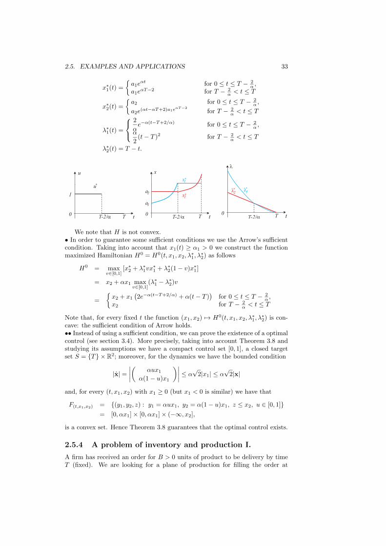
We note that H is not convex.• In order to guarantee some sufficient conditions we use the Arrow’s sufficientcondition. Taking into account that x1(t) ≥ α1 > 0 we construct the functionmaximized Hamiltonian H0 = H0(t, x1, x2, λ
∗1, λ∗2) as follows
H0 = maxv∈[0,1]
[x∗2 + λ∗1vx∗1 + λ∗2(1− v)x∗1]
= x2 + αx1 maxv∈[0,1]
(λ∗1 − λ∗2)v
=
x2 + x1
(2e−α(t−T+2/α) + α(t− T )
)for 0 ≤ t ≤ T − 2
α ,x2 for T − 2
α < t ≤ T
Note that, for every fixed t the function (x1, x2) 7→ H0(t, x1, x2, λ∗1, λ∗2) is con-
cave: the sufficient condition of Arrow holds.•• Instead of using a sufficient condition, we can prove the existence of a optimalcontrol (see section 3.4). More precisely, taking into account Theorem 3.8 andstudying its assumptions we have a compact control set [0, 1], a closed targetset S = T × R2; moreover, for the dynamics we have the bounded condition
|x| =∣∣∣∣( αux1
α(1− u)x1
)∣∣∣∣ ≤ α√2|x1| ≤ α√
2|x|
and, for every (t, x1, x2) with x1 ≥ 0 (but x1 < 0 is similar) we have that
F(t,x1,x2) = (y1, y2, z) : y1 = αux1, y2 = α(1− u)x1, z ≤ x2, u ∈ [0, 1]= [0, αx1]× [0, αx1]× (−∞, x2],
is a convex set. Hence Theorem 3.8 guarantees that the optimal control exists.
2.5.4 A problem of inventory and production I.
A firm has received an order for B > 0 units of product to be delivery by timeT (fixed). We are looking for a plane of production for filling the order at

34 CHAPTER 2. THE SIMPLEST PROBLEM OF OC
the specified delivery data at minimum cost (see [17])11. Let x = x(t) be theinventory accumulated by time t : since such inventory level, at any moment, isthe cumulated past production and taking into account that x(0) = 0, we havethat
x(t) =
∫ t
0
p(s) ds,
where p = p(t) is the production at time t; hence the rate of change of inventoryx is the production and is reasonable to have x = p.
The unit production cost c rises linearly with the production level, i.e. thetotal cost of production is cp = αp2 = αx2; the unit cost of holding inventoryper unit time is constant. Hence the total cost, at time t is αu2 + βx with αand β positive constants, and u = x. Our strategy problem is12
minu
∫ T
0
(αu2 + βx) dt
x = ux(0) = 0x(T ) = B > 0u ≥ 0
(2.76)
Let us consider the Hamiltonian H(t, x, u, λ) = αu2+βx+λu : we are not in thesituation to guarantee that the extremal is normal, but we try! The necessaryconditions are
u∗(t) ∈ arg maxv≥0
(αv2 + βx+ λv) = arg maxv≥0
(αv2 + λv) (2.77)
λ = −β ⇒ λ = −βt+ a, (2.78)
for some constant a. Hence (2.77) gives these situations
y
v
y= v + va l2
-l/(2a)
for l<0 y
v
y= va2
for l=0y
v
y= v + va l2
for l>0
-l a)/(2
11In subsection 5.5.2 we solve the same model with the Dynamic Programming.12We will solve a version of this problem in subsection 5.5.2 with the Dynamic Programming.

2.5. EXAMPLES AND APPLICATIONS 35
This implies
u(t) =
0 if λ(t) ≥ 0
−λ(t)2α if λ(t) < 0
Taking into account (2.78), we have thethree different situations as in the pic-ture here on the right, where τ = a
β .
First, a ≥ Tβ implies u = 0 in [0, T ]and hence, using the initial condition,x = 0 in [0, T ]; this is in contradictionwith x(T ) = B > 0.
Second, 0 < a < Tβ implies
l
t
l=-bt+a, for a<0
T
l=-b bt+a, for 0<a<T
l=-b bt+a, for a>T
t=a/b
u(t) =
0 if 0 ≤ t ≤ τ−λ(t)2α = βt−a
2α = β(t−τ)2α if τ < t ≤ T
Hence, using again the initial condition, x(t) = 0 in [0, τ ] and, using the conti-nuity of x in t = τ,
x(t) =β
4α(t− τ)2 in (τ, T ];
the final condition x(T ) = B gives τ = T − 2√
αBβ . Moreover the condition
0 < a < Tβ gives T > 2√
αBβ .
Finally, the case a ≤ 0 implies u(t) = −λ(t)2α = βt−a2α in [0, T ] and hence
x(t) =β
4αt2 − a
2αt+ d in [0, T ],
for some constant d : the conditions x(0) = 0 and x(T ) = B give
x(t) =β
4αt2 − 4αB − βT 2
4αTt
for T < 2√
αBβ . Summing up, we have
• if T > 2√
αBβ , then with τ = T − 2
√αBβ
u∗(t) =
0 if 0 ≤ t < τβ
2α(t− τ) if τ ≤ t ≤ T and x∗(t) =
0 if 0 ≤ t < τβ
4α(t− τ)
2if τ ≤ t ≤ T
tt
u
T
x
t
t T
B

36 CHAPTER 2. THE SIMPLEST PROBLEM OF OC
• if T ≤ 2√
αBβ , then
u∗(t) =β
2αt+
4αB − βT 2
4αTand x∗(t) =
β
4αt2 +
4αB − βT 2
4αTt
t
u
T
x
t
T
B
In both the cases, we have a normal extremal and a convex Hamiltonian: hencesuch extremals are optimal.
2.6 Singular and bang-bang controls
The Pontryagin Maximum Principle (2.2) gives us, when it is possible, the valueof the u∗ at the point τ ∈ [t0, t1] : more precisely, for every τ ∈ [t0, t1] we arelooking for a unique point w = u∗(τ) belonging to the control set U such that
H(τ,x∗(τ),w, λ∗0,λ∗(τ)) ≥ H(τ,x∗(τ),v, λ∗0,λ
∗(τ)) ∀v ∈ U. (2.79)
In some circumstances, it is possible that using only the PMP can not be foundthe value to assign at u∗ at the point τ ∈ [t0, t1] : examples of this situationwe have found in (2.47), (2.52) and (2.63). Now, let us consider the set T ofthe points τ ∈ [t0, t1] such that PMP gives no information about the value ofthe optimal control u∗ at the point τ, i.e. a point τ ∈ T if and only if there noexists a unique w = w(τ) such that it satisfies (2.79).
We say that an optimal control is singular if T contains some interval of[t0, t1].
In optimal control problems, it is sometimes the case that a control is re-stricted to be between a lower and an upper bound (for example when thecontrol set U is compact). If the optimal control u∗ is such that
u∗(t) ∈ ∂U, ∀t,
we say then that the control is bang-bang. In this case, if u∗ switches from oneextreme to the other at certain times τ , the time τ is called switching point.For example
• in example 2.5.2, we know that the control u∗ in (2.49) is optimal: thevalue of such control is, at all times, on the boundary ∂U = 0, 2 of thecontrol set U = [0, 2]; at time τ = 2− log 3 such optimal control switchesfrom 2 to 0. Hence 2− log 3 is a switching point and u∗ is bang-bang;
• in example 2.5.3, the optimal control u∗ in (2.52) is bang-bang since itsvalue belongs, at all times, to ∂U = 0, 2 of the control set U = [0, 2];the time log 4 is a switching point;

2.6. SINGULAR AND BANG-BANG CONTROLS 37
• in the case B of example 1.1.2, the optimal control u∗ in (2.67) is bang-bang since its value belongs, at all times, to ∂U = 0, 1 of the control setU = [0, 1]; the time T − 1 is a switching point.
2.6.1 The building of a mountain road: a singular control
We have to solve the problem (1.4) presented in example 1.1.3 (see [22] and[17]). We note that there no exist initial or final conditions on the trajectoryand hence we have to satisfy two transversality conditions for the multiplier.The Hamiltonian is H = λ0(x− y)2 + λu, but we try to see if it possible to finda normal extremal, i.e. with λ0 = 1 :
(x∗ − y)2 + λ∗u∗ = minv∈[−α,α]
[(x∗ − y)2 + λ∗v
]⇒ λ∗u∗ = min
v∈[−α,α]λ∗v (2.80)
∂H
∂x= −λ∗ ⇒ λ∗ = −2(x∗ − y)
⇒ λ∗(t) = b− 2
∫ t
t0
(x∗(s)− y(s)) ds, b ∈ R (2.81)
∂H
∂λ= x∗ ⇒ x∗ = u∗ (2.82)
λ∗(t0) = λ∗(t1) = 0 (2.83)
We remark that (2.81) follows from the continuity of y and x. The “minimum”principle (2.80) implies
u∗(t) =
−α for λ∗(t) > 0,α for λ∗(t) < 0,??? for λ∗(t) = 0.
(2.84)
Relations (2.81) and (2.83) give
λ∗(t) = −2
∫ t
t0
(x∗(s)− y(s)) ds, ∀t ∈ [t0, t1] (2.85)∫ t1
t0
(x∗(s)− y(s)) ds = 0. (2.86)
Let us suppose that there exists an interval [c, d] ⊂ [t0, t1] such that λ∗ = 0:clearly by (2.85) we have, for t ∈ [c, d],
0 = λ∗(t)
= 2
∫ c
t0
(x∗(s)− y(s)) ds− 2
∫ t
c
(x∗(s)− y(s)) ds
= λ∗(c)− 2
∫ t
c
(x∗(s)− y(s)) ds ∀t ∈ [c, d]
and hence, since y and x∗ are continuous,
d
dt
(∫ t
c
(x∗(s)− y(s)) ds
)= x∗(t)− y(t) = 0.

38 CHAPTER 2. THE SIMPLEST PROBLEM OF OC
Hence, if λ∗(t) = 0 in [c, d], then x∗(t) = y(t) for all t ∈ [c, d] and, by (2.82),u∗(t) = y(t). We remark that in the set [c, d], the minimum principle has notbeen useful in order to determinate the value of u∗. If there exists such interval[c, d] ⊂ [t0, t1] where λ∗ is null, then the control is singular.
At this point, using (2.84), we are able to conclude that the trajectory x∗
associated to the extremal control u∗ is built with intervals where it coincideswith the ground, i.e. x∗(t) = y(t), and intervals where the slope of the roadis maximum, i.e. x∗(t) ∈ α,−α. Moreover such extremal satisfies (2.86).Finally, we remark that the Hamiltonian is convex with respect to x and u, forevery fixed t : hence the extremal is really a minimum for the problem.
Let us give three examples.
Example A: suppose that |y(t)| ≤ α, ∀t ∈ [t0, t1] :
x
x =y
t
*
t0 t1
l
l*
tt0 t1
We obtain x∗ = y and the control is singular.
Example B: suppose that the slope y of the ground is not contained, for allt ∈ [t0, t1], in [−α, α] :
u
u*
a
t
t0
t1
-a
In the first picture on the left, the dotted line represents the ground y, the solidrepresents the optimal road x∗ : we remark that, by (2.86), the area of the

2.6. SINGULAR AND BANG-BANG CONTROLS 39
region between the two mentioned lines is equal to zero if we take into accountthe “sign” of such areas. The control is singular.
Example 2.6.1. Suppose that the equation of the ground is x(t) = et for t ∈ [−1, 1] andthe slope of such road must satisfy |x(t)| ≤ 1.
We have to solve minu
∫ 1
−1(x− et)2 dt
x = u−1 ≤ u ≤ 1
We know, for the previous consideration and calculations, that for every t ∈ [−1, 1]
• one possibility is that x∗(t) = y(t) = et and λ(t) = 0, |x∗(t)| = |u∗(t)| ≤ 1,
• the other possibility is that x∗(t) = u∗(t) ∈ −1,+1.We note that for t > 0 the second possibility can not happen because y(t) > 1. Hence let usconsider the function
x∗(t) =
et for t ∈ [−1, α],t+ eα − α for t ∈ (α, 1],
with α ∈ (−1, 0) such that (2.86) is satisfied:
x
t-1 1
y
x*
1
1
a
∫ 1
−1(x∗(s)− y(s)) ds =
∫ 1
α(s+ eα − α− es) ds
=1
2+ 2eα +
1
2α2 − e− α− αeα = 0. (2.87)
For the continuous function h : [−1, 0]→ R, defined by
h(t) =1
2+ 2et +
1
2t2 − e− t− tet,
we have
h(−1) =−e2 + 2e+ 3
e= −
(e− 3)(e+ 1)
e> 0
h(0) =5
2− e < 0,
certainly there exists a point α ∈ (−1, 0) such that h(α) = 0 and hence (2.87) holds. Moreover,since h′(t) = (et − 1)(1− t) < 0 in (0, 1), such point α is unique. Using (2.85), we are able todeterminate the multiplier:
λ∗(t) =
0 if t ∈ [−1, α]
−2
∫ t
α(s+ eα − α− es)ds =
=1
2(t2 − α2) + (eα − α)(t− α) + eα − et if t ∈ (α, 1]
Note that in the interval [−1, α] the PMP in (2.80) becomes
0 = minv∈[−1,1]
0
and gives us no information. Hence u∗ is singular. 4
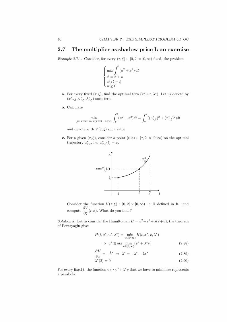
40 CHAPTER 2. THE SIMPLEST PROBLEM OF OC
2.7 The multiplier as shadow price I: an exercise
Example 2.7.1. Consider, for every (τ, ξ) ∈ [0, 2]× [0,∞) fixed, the problemmin
∫ 2
τ
(u2 + x2) dt
x = x+ ux(τ) = ξu ≥ 0
a. For every fixed (τ, ξ), find the optimal tern (x∗, u∗, λ∗). Let us denote by(x∗τ,ξ, u
∗τ,ξ, λ
∗τ,ξ) such tern.
b. Calculate
minu: x=x+u, x(τ)=ξ, u≥0
∫ 2
τ
(u2 + x2)dt =
∫ 2
τ
((u∗τ,ξ)2 + (x∗τ,ξ)
2)dt
and denote with V (τ, ξ) such value.
c. For a given (τ, ξ), consider a point (t, x) ∈ [τ, 2] × [0,∞) on the optimaltrajectory x∗τ,ξ, i.e. x∗τ,ξ(t) = x.
x
t2t
x
x x* t= ( )t,x
x*t,x
t
Consider the function V (τ, ξ) : [0, 2] × [0,∞) → R defined in b. and
compute∂V
∂ξ(t, x). What do you find ?
Solution a. Let us consider the Hamiltonian H = u2+x2+λ(x+u); the theoremof Pontryagin gives
H(t, x∗, u∗, λ∗) = minv∈[0,∞)
H(t, x∗, v, λ∗)
⇒ u∗ ∈ arg minv∈[0,∞)
(v2 + λ∗v) (2.88)
∂H
∂x= −λ∗ ⇒ λ∗ = −λ∗ − 2x∗ (2.89)
λ∗(2) = 0 (2.90)
For every fixed t, the function v 7→ v2+λ∗v that we have to minimize representsa parabola:
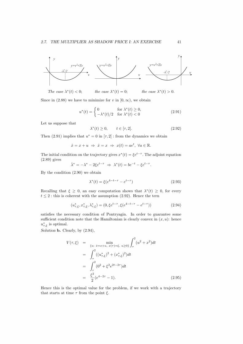
2.7. THE MULTIPLIER AS SHADOW PRICE I: AN EXERCISE 41
y
v- /2l
*
y=v + vl2 *
y
v
y=v + vl2 *
y
v
y=v + vl2 *
- /2l*
The case λ∗(t) < 0; the case λ∗(t) = 0; the case λ∗(t) > 0.
Since in (2.88) we have to minimize for v in [0,∞), we obtain
u∗(t) =
0 for λ∗(t) ≥ 0,−λ∗(t)/2 for λ∗(t) < 0
(2.91)
Let us suppose that
λ∗(t) ≥ 0, t ∈ [τ, 2]. (2.92)
Then (2.91) implies that u∗ = 0 in [τ, 2] : from the dynamics we obtain
x = x+ u ⇒ x = x ⇒ x(t) = aet, ∀a ∈ R.
The initial condition on the trajectory gives x∗(t) = ξet−τ . The adjoint equation(2.89) gives
λ∗ = −λ∗ − 2ξet−τ ⇒ λ∗(t) = be−t − ξet−τ .
By the condition (2.90) we obtain
λ∗(t) = ξ(e4−t−τ − et−τ ) (2.93)
Recalling that ξ ≥ 0, an easy computation shows that λ∗(t) ≥ 0, for everyt ≤ 2 : this is coherent with the assumption (2.92). Hence the tern
(u∗τ,ξ, x∗τ,ξ, λ
∗τ,ξ) = (0, ξet−τ , ξ(e4−t−τ − et−τ )) (2.94)
satisfies the necessary condition of Pontryagin. In order to guarantee somesufficient condition note that the Hamiltonian is clearly convex in (x, u): henceu∗τ,ξ is optimal.
Solution b. Clearly, by (2.94),
V (τ, ξ) = minu: x=x+u, x(τ)=ξ, u≥0
∫ 2
τ
(u2 + x2)dt
=
∫ 2
τ
((u∗τ,ξ)2 + (x∗τ,ξ)
2)dt
=
∫ 2
τ
(02 + ξ2e2t−2τ )dt
=ξ2
2(e4−2τ − 1). (2.95)
Hence this is the optimal value for the problem, if we work with a trajectorythat starts at time τ from the point ξ.

42 CHAPTER 2. THE SIMPLEST PROBLEM OF OC
Solution c. Since
V (τ ′, ξ′) =(ξ′)2
2(e4−2τ
′− 1),
we have∂V
∂ξ(τ ′, ξ′) = ξ′(e4−2τ
′− 1).
In particular, if we consider a point (t, x) ∈ [τ, 2] × [0,∞) on the optimal tra-jectory x∗τ,ξ, i.e. using (2.94) the point (t, x) is such that
x = x∗τ,ξ(t) = ξet−τ ,
we obtain∂V
∂ξ(t, x) = ξet−τ (e4−2t − 1) = ξ(e4−t−τ − et−τ ).
Hence we have found that
∂V
∂ξ(t, x∗τ,ξ(t)) = λ∗τ,ξ(t),
i.e.
Remark 2.11. The multiplier λ∗, at time t, expresses the sensitivity, the “shadowprice”, of the optimal value of the problem when we modify the initial data ξ,along the optimal trajectory.
We will see in theorem 5.9 that this is a fundamental property that holds in thegeneral context and links the multiplier λ∗ of the variational approach to thevalue function V of the dynamic programming. Two further comments on theprevious exercise:
1. The function V (τ, ξ) : [0, 2] × [0,∞) → R is called value function and isthe fundamental object of the dynamic programming. One of its propertyis that V (2, ξ) = 0, ∀ξ.
2. Consider the points (τ, ξ) and (τ ′, ξ′) in [0, 2]× [0,∞) : we know that theoptimal trajectories are
x∗τ,ξ(t) = ξet−τ , x∗τ ′,ξ′(t) = ξ′et−τ′.
Now consider (τ ′, ξ′) on the optimal trajectory x∗τ,ξ, i.e. the point (τ ′, ξ′)is such that
ξ′ = x∗τ,ξ(τ′) = ξeτ
′−τ .
The previous expressions give us that, with this particular choice of (τ ′, ξ′)
x∗τ ′,ξ′(t) = ξ′et−τ′
= ξeτ′−τet−τ
′= ξet−τ = et−τ
′= x∗τ,ξ(t).
Hence the optimal trajectory associated to the initial data (τ ′ξ′) (with(τ ′ξ′) that belongs to the optimal trajectory associated to the initial data(τ, ξ)), coincides with the optimal trajectory associated to the initial data(τ, ξ). We will see that this is a fundamental property that holds in general:“the second part of an optimal trajectory is again otpimal” is the Principleof Bellman of dynamic programming (see Theorem 5.1).

Chapter 3
General problems of OC
In this chapter we will see more general problem then (2.1). In the literaturethere are many books devoted to this study (see for example [27], [19], [25], [5],[26]): however, the fundamental tool is the Theorem of Pontryagin that gives anecessary and useful condition of optimality.
3.1 Problems of Bolza, of Mayer and of Lagrange
Starting from the problem (2.1), let us consider t0 fixed and T be fixed or free,with T > t0. The problem
J(u) = ψ(T,x(T ))x = g(t,x,u)x(t0) = αmaxu∈C
J(u),
(3.1)
with ψ : [t0,∞)× Rn → R, is called OC problem of Mayer. The problemJ(u) =
∫ T
t0
f(t,x,u) dt+ ψ(T,x(T ))
x = g(t,x,u)x(t0) = αmaxu∈C
J(u),
(3.2)
is called OC of Bolza. The problemJ(u) =
∫ T
t0
f(t,x,u) dt
x = g(t,x,u)x(t0) = αmaxu∈C
J(u),
(3.3)
is called OC of Lagrange. We have the following result
Remark 3.1. The problems (3.1), (3.2) e (3.3) are equivalent.
43

44 CHAPTER 3. GENERAL PROBLEMS OF OC
Clearly the problems (3.1) and (3.3) are particular cases of (3.2).First, let us show how (3.2) can become a problem of Lagrange: since∫ T
t0
f(t,x,u) dt+ψ(T,x(T )) =
∫ T
t0
(f(t,x,u) +
dψ(t,x(t))
dt
)dt−ψ(t0,x(t0))
problem (3.2) becomesJ(u) =
∫ T
t0
(f(t,x,u) +
∂ψ
∂t(t,x) +∇xψ(t,x) · g(t,x,u)
)dt
x = g(t,x,u)x(t0) = αmaxu∈C
J(u)
that is clearly of Lagrange.Secondly, let us proof how (3.3) can become a problem of Mayer: we intro-
duce the new variable xn+1 defined by xn+1(t) = f(t,x,u) with the conditionxn+1(t0) = 0. Since
xn+1(T ) = xn+1(t0) +
∫ T
t0
f(t,x,u) dt,
problem (3.3) becomesJ(u) = xn+1(T )(x, xn+1) = (g(t,x,u), f(t,x,u))(x(t0), xn+1(t0)) = (α, 0)maxu∈C
J(u)
that is of Mayer.Finally, we show how the problem (3.1) becomes a problem of Lagrange: let
us introduce the variable xn+1 as xn+1(t) = 0 with the condition xn+1(T ) =
xn+1(t0) = ψ(T,x(T ))T−t0 . Problem (3.1) becomes
J(u) =
∫ T
t0
xn+1 dt
(x, xn+1) = (g(t,x,u), 0)x(t0) = α
xn+1(t0) = ψ(T,x(T ))T−t0
maxu∈C
J(u)
that is of Lagrange.
3.2 Problems with fixed or free final time
3.2.1 Fixed final time
Let us consider f : [t0, t1] × Rn+k → R, ψ : Rn → R and let α ∈ Rn be fixed.Let x = (x1, x2, . . . , xn) and let n1, n2 and n3 be non negative, fixed integer

3.2. PROBLEMS WITH FIXED OR FREE FINAL TIME 45
such that n1 + n2 + n3 = n. Let us consider the problem
maxu∈C
∫ t1
t0
f(t,x,u) dt+ ψ(x(t1))
x = g(t,x,u)x(t0) = αxi(t1) free 1 ≤ i ≤ n1xj(t1) ≥ βj with βj fixed n1 + 1 ≤ j ≤ n1 + n2xl(t1) = βl with βl fixed n1 + n2 + 1 ≤ l ≤ n1 + n2 + n3C = u : [t0, t1]→ U ⊆ Rk, u admissible
(3.4)
where t0 and t1 are fixed. Since xi(t1) is fixed for n− n3 < i ≤ n, then the payoff function ψ depends only on xi(t1) with 1 ≤ i ≤ n− n3.We have the following necessary condition, a generalization theorem 2.1 of Pon-tryagin:
Theorem 3.1. Let us consider the problem (3.4) with f ∈ C1([t0, t1]×Rn+k), g ∈C1([t0, t1]× Rn+k) and ψ ∈ C1(Rn).Let u∗ be optimal control and x∗ be the associated trajectory.Then there exists a multiplier (λ∗0,λ
∗), with
λ∗0 ≥ 0 constant,
λ∗ : [t0, T∗]→ Rn continuous,
such that
i) the nontriviality of the multiplier holds;
ii) the Pontryagin Maximum Principle (2.2) holds,
iii) the adjoint equation (2.3) holds,
ivt1) the transversality condition is given by
• for 1 ≤ i ≤ n1, we have λ∗i (t1) = λ∗0∂ψ
∂xi(x∗(t1)),
• for n1 + 1 ≤ j ≤ n1 +n2, we have λ∗j (t1) ≥ λ∗0∂ψ
∂xj(x∗(t1)), x∗j (t1) ≥
βj and
(λ∗j (t1)− λ∗0
∂ψ
∂xj(x∗(t1))
)(x∗j (t1)− βj
)= 0.
We will give an idea of the proof in Theorem 3.4.Using Remark 3.1, it is clear that a problem with final time fixed and value
of the trajectory in such final time free, it is possible to guarantee the normalityof the control as in Theorem 2.1. More precisely
Remark 3.2. Let us consider the problem (3.4) with n2 = n3 = 0, i.e. x(t1)free. Then in Theorem 3.1 it is possible to guarantee that u∗ is normal, i.e.λ∗0 = 1.
A sufficient condition for the problem (3.4), with a proof similar to the onein theorem 2.3, is the following:

46 CHAPTER 3. GENERAL PROBLEMS OF OC
Theorem 3.2. Let us consider the maximum problem (3.4) with f, g and ψin C1. Let the control set U be convex. Let u∗ be a normal admissible control;let x∗ and (1,λ∗) be the associated trajectory and multiplier respectively. Wesuppose that all the necessary conditions of theorem 3.1 hold.Moreover, we suppose that
v) the functions (x,u) 7→ H(t,x,u,λ∗) and x 7→ ψ(x) are concave functionsin the variables x and u, for all t ∈ [t0, t1] fixed.
Then u∗ is optimal.
We mention that the sufficient condition of Arrow works in this more generalsituation (see Theorem 3.4 in [26]).
Autonomous problems
It is clear that the arguments of subsection 2.1 are true. Hence
Remark 3.3. In the assumption of Theorem 3.1, if the problem is autonomous,then we have that in [t0, t1] (2.11) is true, i.e.
H(x∗(t),u∗(t), λ∗0,λ∗(t)) = constant
3.2.2 Free final time
Let us consider f : [t0,∞) × Rn+k → R, g : [t0,∞) × Rn+k → R and ψ :[t0,∞)×Rn → R, and let α ∈ Rn be fixed. Let x = (x1, x2, . . . , xn) and n1, n2
and n3 be non negative, fixed integer such that n1 + n2 + n3 = n. We considerthe problem
maxu∈C
∫ T
t0
f(t,x,u) dt+ ψ(T,x(T ))
x = g(t,x,u)x(t0) = αxi(T ) free 1 ≤ i ≤ n1xj(T ) ≥ βj with βj fixed n1 + 1 ≤ j ≤ n1 + n2xl(T ) = βl with βl fixed n1 + n2 + 1 ≤ l ≤ n1 + n2 + n3C = u : [t0,∞)→ U ⊆ Rk, u admissible
(3.5)
where t0 is fixed and T is free with T > t0. We say that u∗ is optimal with exittime T ∗ if∫ T∗
t0
f(t,x∗,u∗) dt+ ψ(T ∗,x∗(T ∗)) ≥∫ T
t0
f(t,x,u) dt+ ψ(T,x(T ))
for every admissible control u and for every T ≥ t0. Hence and optimal controlhas an (unique) associated exit time. We have the following result, again ageneralization of the theorem of Pontryagin 2.1 (see [22]):
Theorem 3.3. Let us consider the problem (3.5) with f ∈ C1([t0,∞)×Rn+k), g ∈C1([t0,∞)× Rn+k) and ψ ∈ C1([t0,∞)× Rn).Let u∗ be optimal control with exit time T ∗ and x∗ be the associated trajectory.
Then there exists a multiplier (λ∗0,λ∗), with

3.2. PROBLEMS WITH FIXED OR FREE FINAL TIME 47
λ∗0 ≥ 0 constant,
λ∗ : [t0, t1]→ Rn continuous,
such that
i) the nontriviality of the multiplier holds;
ii) the Pontryagin Maximum Principle (2.2) holds,
iii) the adjoint equation (2.3) holds,
ivT∗) the transversality condition is given by
• for 1 ≤ i ≤ n1, we have λ∗i (T∗) = λ∗0
∂ψ
∂xi(T ∗,x∗(T ∗)),
• for n1 + 1 ≤ j ≤ n1 + n2, we have λ∗j (T∗) ≥ λ∗0
∂ψ
∂xj(T ∗,x∗(T ∗)),
x∗j (T∗) ≥ βj ,
(λ∗j (T
∗)− λ∗0∂ψ
∂xj(T ∗,x∗(T ∗))
)(x∗j (T
∗)− βj)
= 0;
moreover we have
H(T ∗,x∗(T ∗),u∗(T ∗), λ∗0,λ∗(T ∗)) + λ∗0
∂ψ
∂t(T ∗,x∗(T ∗)) = 0. (3.6)
We will give an idea of the proof in Theorem 3.4.For variable time optimal problems it is hard to find sufficient conditions
of any practical value, due to an inherent lack of convexity properties in suchproblems.
Remark 3.4. In the context of problem (3.5) with convex control set U , theregularity and the concavity of the Hamiltonian and the normality of the extremalare not sufficient conditions of optimality, i.e. a result similar to Theorem 3.2does not hold in this new situation.
In [26] appear some sufficient conditions for a large type of problems: in thisnote we prefer to provide some necessary conditions for the particular problemsthat we present and some existence results of the optimal control (see section3.4).
Autonomous problems
In the particular case of a autonomous problem with free final time the argu-ments of subsection 2.1 are true. Hence, using condition (3.6), we have
Remark 3.5. In the assumption of Theorem 3.3, if the problem is autonomous,then we have that
H(x∗(t),u∗(t), λ∗0,λ∗(t)) = 0 t ∈ [t0, T
∗]; (3.7)
More details can be found in, for example, [26] (page 172) and [1] (page 189).

48 CHAPTER 3. GENERAL PROBLEMS OF OC
3.2.3 The proof of the necessary condition
In this subsection our aim is to give an idea of the proof of the generalizationof Pontryagin theorem presented in theorems 3.1 and 3.3. More precisely weprove, in the spirit of the previous theorem 2.2 and in the case n = k = 1, thefollowing:
Theorem 3.4. Let us consider the problem
J(u) =
∫ T
t0
f(t, x, u) dt+ ψ(T, x(T ))
x = g(t, x, u)x(t0) = α fixedmaxu∈C
J(u)
C =u : [t0, T ]→ R, u ∈ C([t0, T ]), T > t0
(3.8)
with f and g in C1, and C open and non empty. Moreover, in the problem (3.8)we require one of the following four situations:
I. T is fixed1 and x(T ) = β is fixed;
II. T is fixed1 and x(T ) = β is free;
III. T is free and x(T ) = β is fixed;
IV. T is free and x(T ) = β is free.
Let u∗ be the optimal control with exit time T ∗ and x∗ be the optimal trajectory.Then there exists a multiplier (λ∗0, λ
∗), with
λ∗0 constant,
λ∗ : [t0, T∗]→ R continuous,
such that (λ∗0, λ∗) 6= (0, 0) and
i) the PMP0∂H
∂u(t, x∗(t), u∗(t), λ∗0, λ
∗(t)) = 0 holds,
ii) the adjoint equation (2.3) holds,
iiiT∗) the transversality condition, depending on the previous situations, is
I. no condition;
II. we have λ∗(T ∗) = λ∗0∂ψ
∂x(x∗(T ∗));
III. we have
H(T ∗,x∗(T ∗),u∗(T ∗), λ∗0,λ∗(T ∗)) + λ∗0
∂ψ
∂t(T ∗,x∗(T ∗)) = 0; (3.9)
IV. we have λ∗(T ∗) = λ∗0∂ψ
∂x(T ∗,x∗(T ∗)) and (3.9).
1Note that in this case ψ(t, x) = ψ(x).

3.2. PROBLEMS WITH FIXED OR FREE FINAL TIME 49
iv) λ∗0 ≥ 0.
Proof. First, let us proof the case IV. As in the proof of theorem 2.2, let
u∗ ∈ C be optimal control with exit time T ∗ and x∗ its trajectory. Let us fixa continuous function h : [t0,∞) → R. For every constant ε ∈ R we define thefunction uε = u∗ + εh. Moreover, we consider a generic C1 exit time functionT (ε) = Tε : R → [t0,∞) such that T0 = T ∗. Hence, for every ε-variation of thetern (u∗, x∗, T ∗) we have a new tern (uε, xε, Tε) where xε : [0, Tε]→ R is thetrajectory associated to uε : [0, Tε]→ R. Clearly
T (0) = T ∗, xε(t0) = α fixed,
xε(Tε) = βε, x0(t) = x∗(t).
Now, recalling that h is fixed and considering a constant λ0 ≥ 0, we define thefunction Jh : R→ R as
Jh(ε) = λ0
(∫ Tε
t0
f(t, xε(t), uε(t)
)dt+ ψ(Tε, βε)
).
Let λ : [t0,∞)→ R be a generic continuous function: we obtain
Jh(ε) =
∫ T (ε)
t0
λ0f
(t, xε, uε
)+ λ(g(t, xε, uε
)− xε
)dt+ λ0ψ(Tε, βε)
(by part) =
∫ Tε
t0
H(t, xε, uε, λ0, λ) + λxε
dt−
(λ(Tε)βε − λ(t0)α
)+
+λ0ψ(Tε, βε)
Since u∗ is optimal and λ0 ≥ 0, we have dJhdε (0) = 0. Hence2
dJhdε
(0) =
∫ T∗
t0
[∂H
∂x(t, x∗, u∗, λ0, λ) + λ
]dxεdε
(0) +∂H
∂u(t, x∗, u∗, λ0, λ)h
dt+
+
[H(T ∗, x∗(T ∗), u∗(T ∗), λ0, λ(T ∗)) + λ0
∂ψ
∂t(T ∗, x∗(T ∗))
]dTεdε
(0) +
−[λ(T ∗)− λ0
∂ψ
∂x(T ∗, x∗(T ∗))
]dβεdε
(0)
= 0. (3.10)
Clearly Tε and xε(Tε) = βε are free and we have no information on dTεdε (0) and
dβεdε (0). Hence we require that λ0 and λ solve the systemλ(t) = −λ(t)
∂g
∂x(t, x∗, u∗)− λ0
∂f
∂x(t, x∗, u∗) in [t0, T
∗]
λ(T ∗) = λ0∂ψ
∂x(T ∗, x∗(T ∗))
λ0f(T ∗, x∗(T ∗), u∗(T ∗)) + λ(T ∗)g(T ∗, x∗(T ∗), u∗(T ∗)) + λ0∂ψ
∂t(T ∗, x∗(T ∗)) = 0
2We recall that
Proposition 3.1. Let α and β in C1([a, b]), with a < b, such that α(ε) ≤ β(ε), for everyε ∈ [a, b]. Let A = (t, ε) : ε ∈ [a, b], α(ε) ≤ t ≤ β(ε) and consider the function g : A → R.We suppose that g and ∂g
∂εare continuous in A. Then
d
dε
∫ β(ε)
α(ε)g(t, ε) dt =
∫ β(ε)
α(ε)
∂g
∂ε(t, ε) dt+ β′(ε)g(β(ε), ε)− α′(ε)g(α(ε), ε).

50 CHAPTER 3. GENERAL PROBLEMS OF OC
Considering the last two conditions in the point T ∗ we obtain
λ0
(f(T ∗, x∗(T ∗), u∗(T ∗)) +
∂ψ
∂x(T ∗, x∗(T ∗))g(T ∗, x∗(T ∗), u∗(T ∗)) +
+∂ψ
∂t(T ∗, x∗(T ∗))
)= 0 :
Clearly, if the big parenthesis is different from zero, then λ∗0 = 0; if the bigparenthesis is zero, then we set λ∗0 = 1. Note that in both cases there exists asolution λ∗ of the previous ODE and the two transversality conditions.3 Forthese choices of the function λ = λ∗ and of the constant λ0 = λ∗0, we have by(3.10) ∫ T∗
t0
∂H
∂u(t, x∗, u∗, λ∗0, λ
∗)hdt = 0, (3.11)
for every h ∈ C([t0,∞)). Lemma 2.2 gives the PMP0.The proof of case I. is similar; here T (ε) = T ∗ and xε(T (ε)) = β are fixed
and hencedT
dε(0) = 0,
dβ
dε(0) = 0.
No transversality conditions appear in this case.The other two cases are similar.
3.2.4 The moonlanding problem
The formulation of the problem presented in (1.7) is the following:
maxu∈C
m(T )
h = vv =
u
m− g
m = −kuh(0) = h0, h(T ) = 0v(0) = v0, v(T ) = 0m(0) = M + Fm(t) ≥ 0, h(t) ≥ 0C = u : [0, T ]→ [0, α], admissible
where h0, M, F, g, −v0, k and α are positive and fixed constants; the finaltime T is free. The target set for the problem is S = [0,∞)× (0, 0) × [0,∞).First of all we remark that a reasonable assumption is
α > g(M + F ) (3.12)
i.e. the possibility for the spacecraft to win the gravitation acceleration of themoon.
The Hamiltoniana is
H(h, v,m, u, λ0, λ1, λ2, λ3) = λ1v + λ2
( um− g)− λ3ku
3We mention that our proof is incomplete: we omit to prove that (λ∗0, λ∗) 6= (0, 0).
3.2. PROBLEMS WITH FIXED OR FREE FINAL TIME 51
with a pay off function
ψ(h, v,m) = m.
Theorem 3.1 implies
u(t) ∈ arg maxw∈[0,α]
(λ1(t)v(t) + λ2(t)
(w
m(t)− g)− λ3(t)kw
)
⇒ u(t) =
α if λ2(t)
m(t) − λ3(t)k > 0
? if λ2(t)m(t) − λ3(t)k = 0
0 if λ2(t)m(t) − λ3(t)k < 0
(3.13)
λ1 = −∂H∂h
⇒ λ1 = 0 ⇒ λ1(t) = a
λ2 = −∂H∂v
⇒ λ2 = −λ1 ⇒ λ2(t) = −at+ b (3.14)
λ3 = −∂H∂m
⇒ λ3 =λ2u
m2(3.15)
λ3(T ) = λ0∂ψ
∂m(m(T )) ⇒ λ3(T ) = λ0
where a and b are constants. Moreover, since the problem is autonomous, (3.7)implies
λ1(t)v(t) + λ2(t)
(u(t)
m(t)− g)− λ3(t)ku(t) = 0, ∀t ∈ [0, T ] (3.16)
Let us suppose that a = b = 0: we easily obtain λ1 = λ2 = 0 and λ3 = λ0in [0, T ]. The case λ0 = 0 contradicts the nontriviality of the multiplier; thenλ0 6= 0. The case λ0 6= 0 gives, using (3.16),
u(t) = 0 in [0, T ] : (3.17)
clear this is unreasonable: however, from a mathematical point of view, thedynamics gives v = −g which contradicts v(0) = v0 < 0, v(T ) = 0.
Now, let us suppose that a and b are not both zero: we prove that there
exists at most one point τ ∈ [0, T ] such that in (3.13) we have λ2(τ)m(τ) −λ3(τ)k = 0.
In order to do that, we define the function φ : [0, T ]→ R by
φ(t) =λ2(t)
m(t)− λ3(t)k.
Using the dynamics, (3.14) and (3.15) we obtain
φ =λ2m− λ2m
m2− λ3k = − a
m;
this proves that φ is monotone. We have to show that the case a = 0 = φ andφ = 0 in [0, T ] does not occur; clearly φ = 0 implies λ3 = b
km in all [0, T ]. Thisrelation and a = 0 in (3.16) imply b = 0: we know that a = b = 0 it’s impossible.Hence, really there exists at most one point τ ∈ [0, T ] such that φ(τ).

52 CHAPTER 3. GENERAL PROBLEMS OF OC
Now we have four possibilities for the extremal control u
I u(t) =
0 for t ∈ [0, τ ]α for t ∈ (τ, T ]
II u(t) =
α for t ∈ [0, τ ]0 for t ∈ (τ, T ]
III u(t) = 0 for t ∈ [0, T ] IV u(t) = α for t ∈ [0, T ]
Case IV is a.e. a particular case of case I with τ = 0. Case III is as in(3.17). Case II is unreasonable: however, from a mathematical point of view,the dynamics gives v(T ) = −g which implies, taking into account v(T ) = 0,that there exists t′ such that v(t) > 0 for t ∈ (t′, T ). Now the relation
h(t) = h(T ) +
∫ t
T
v(s) ds,
taking into account h(T ) = 0, implies h(t) < 0 for t ∈ (t′, T ).Hence we focus our attention on the Case I. In [0, τ ] the dynamics and the
initial conditions give h(t) = − t
2g
2+ v0t+ h0
v(t) = −tg + v0m(t) = M + F
(3.18)
In the (v, h)-plane, the previous relations gives the free fall curve γ
h = −v2
2g+v202g
+ h0; (3.19)
its interpretation is that if the spacecraft starts at the (v0, h0)-point (recall thatv0 < 0, h0 > 0), the corresponding curve in (3.19) describes the free fall, i.e.with u = 0: we notice that v decreases.
In the interval [τ, T ], putting u(t) = α in the dynamics we obtain
m = −ku ⇒ m(t) = m(τ)− (t− τ)kα
mv(t) = u−mg ⇒ v =α
m(τ)− (t− τ)kα− g
⇒ v(t) = −1
klog
(m(τ)− (t− τ)kα
m(τ)
)− (t− τ)g + v(τ)
h = v ⇒ h(t) =
∫ t
τ
v(s) ds+ h(τ)
We remark that, by (3.12), we have
α
m(τ)− (t− τ)kα− g ≥ α
M + F− g > 0
and hence M + F − (t − τ)kα > 0. By using (3.18) and the continuity of thetrajectory
h(t) =M + F − (t− τ)kα
k2αlog
(M + F − (t− τ)kα
M + F
)+
+t− τk− (t− τ)2g
2+ (t− τ)v(τ) + h(τ)
v(t) = −1
klog
(M + F − (t− τ)kα
M + F
)− (t− τ)g + v(τ)
m(t) = M + F − (t− τ)kα.
(3.20)

3.2. PROBLEMS WITH FIXED OR FREE FINAL TIME 53
Since in the final point T we have h(T ) = v(T ) = 0 and setting s = T − τ , theprevious equations for h and v become
0 =M + F − skα
k2αlog
(M + F − skα
M + F
)+s
k− s2g
2+ sv(τ) + h(τ)
0 = −1
klog
(M + F − skα
M + F
)− sg + v(τ)
and hencev(s) := v(τ) =
1
klog
(M + F − skα
M + F
)+ gs
h(s) := h(τ) = −M + F
k2αlog
(M + F − skα
M + F
)− s
k− s2g
2
(3.21)
The previous arguments say that τ is exactly the time necessary for a spacecraftthat has a initial state (v(τ), h(τ)) to arrive on the moon with velocity zero.Hence in (3.21) we have a curve s 7→ γ(s) = (v(s), h(s)): from the constructionof this curve (usually called switching curve), its interpretation is that if thespacecraft is at a (v, h)-point on the curve corresponding to the parameter sand if it thrusts at maximum rate α, then it will arrive at v = 0, h = 0 in times. Finally, we remark that the spacecraft burns fuel at rate kα; since the totalamount of fuel is F we have the condition 0 ≤ s ≤ F
kα in our switching curve.The initial data (v0, h0) in the interiorof the reachable set R. The free fallcurve γ in (3.19) and the switchingcurve in (3.21). The point P = γ ∩ γ:the switching point τ is such that P =γ(τ); finally, if s is such that P = γ(s),then the final time T is T = τ + s.In order to draw the curve γ note thatγ(0) = (v(0), h(0)) = (0, 0) and that(3.12) implies
v′(s) = − α
M + F − skα − g < 0
and
h′(s) =M + F
k(M + F − skα) −1
k− sg
= s
(α
M + F − skα − g)> 0.
It is clear from the previous picture that for some initial data (v0, h0) there is nosolution for the problem; moreover for every initial data (v0, h0) in the interiorof the reachable set, there exists a unique switching point τ ∈ [0, T ]; the secondpart of the trajectory lies on the switching curve and spends exactly a time sto arrive in the origin. Hence T = τ + s.
Now let us prove that the above construction give an extremal. The controlis
u(t) =
0 for t ∈ [0, τ ]α for t ∈ (τ, T ]
(3.22)

54 CHAPTER 3. GENERAL PROBLEMS OF OC
and the associated trajectory is given by (3.18) for t ∈ [0, τ ] and by (3.20) fort ∈ (τ, T ]. Note that such trajectory is uniquely determined by the initial data;moreover we found τ and T .The multiplier is given by
λ1(t) = a, λ2(t) = −at+ b, λ3(t) =
c if t ∈ [0, τ ]
λ0 − α∫ T
t
−as+ b
(m(s))2ds if t ∈ (τ, T ]
Since m(s) > 0, the last integral exists and is finite in [τ, T ]. By the continuitywe have
c = λ0 − α∫ T
τ
−as+ b
(m(s))2ds (3.23)
We recall that τ is such that φ(τ): hence
−aτ + b
M + F− ck = 0 (3.24)
Relation (3.16) implies4
0 = av0 − bg (for t = 0) (3.25)
0 = (−aT + b)
(α
m(T )− g)− λ0kα (for t = T ) (3.26)
Now
(3.25) ⇒ a =bg
v0(3.27)
(3.26) ⇒ λ0 =b
kα
(− g
v0T + 1
)(α
m(T )− g)
(3.28)
(3.24) ⇒ c =b
k(M + F )
(− g
v0τ + 1
)(3.29)
(3.23) ⇒ c = b
[1
kα
(− g
v0T + 1
)(α
m(T )− g)− α
∫ T
τ
− gv0s+ 1
(m(s))2ds
](3.30)
Clearly − gv0T + 1 is positive and (3.12) implies α
m(T ) − g > 0; hence if λ0 = 0,
then (3.28) implies b = 0; now (3.27) and (3.29) imply a = c = 0; finally weobtain λ3 = 0. This is impossible by the non triviality of the multiplier.Hence we put λ0 = 1 and it is easy to see that there exists unique (a, b, c) suchthat relations (3.27)–(3.30) are true. We have only to mention that relations(3.29) and (3.30) are not in contradiction.5 Hence we have that u in (3.22) is anormal extremal control.
4It is easy to see that, using (3.24), relation (3.16) for t = τ doesn’t give new information.5 We have
1
kα
(−g
v0T + 1
)(α
m(T )− g)−
1
k(M + F )
(−g
v0τ + 1
)− α
∫ T
τ
− gv0s+ 1
(m(s))2ds =
=1
k
[(−g
v0T + 1
)(1
m(T )−g
α
)−
1
M + F
(−g
v0τ + 1
)−∫ T
τ
(−g
v0s+ 1
)−m(s)
(m(s))2ds
]=
1
k
[−g
α
(−g
v0T + 1
)+
∫ T
τ−g
v0
1
m(s)ds
]

3.3. THE BOLZA PROBLEM IN CALCULUS OF VARIATIONS. 55
Now, we can apply a generic result of the existence of an optimal control(see Theorem 3.8). We know, by the previous construction, that there existsat least an admissible control u with exit time T ; hence it is reasonable torestrict the original target set S = [0,∞) × (0, 0) × [0,∞) to the new setS = [0, T ] × (0, 0) × [0,∞). Moreover, we have a compact control set [0, α]and for the dynamics we have the bounded condition∣∣∣∣∣∣
h
v
m
∣∣∣∣∣∣ =
∣∣∣∣∣∣ v
u/m− g−ku
∣∣∣∣∣∣≤
√v2 +
α2
M2+ g2 + k2α2
≤√
α2
M2+ g2 + k2α2 + |v|
≤ (1 + C)(1 + |(h, v,m)′|);
finally, for every (t, h, v,m) we have that
F(t,h,v,m) =
(y1, y2, y3, z) : y1 = v, y2 =u
m− g, y3 = −ku, z ≤ 0, u ∈ [0, α]
is a convex set. Hence Theorem 3.8 guarantees that the optimal control exists.
3.3 The Bolza problem in Calculus of Variations.
Let us consider the problem
J(x) =
∫ T
t0
f(t,x(t), x(t)) dt+ ψ(T,x(T ))
x(t0) = αx(T ) = βTmaxx∈AB
J(x)
AB = x : [t0,∞)→ Rn, x ∈ C1, x(t0) = α
(3.31)
where t0 is fixed, and T > t0, βT ∈ Rn are free. We call this problem Bolzaproblem of calculus of variation. Clearly (3.31) is a particular case of (3.5), butlet us provide the necessary condition for this particular situation: hence, let usapply theorem 3.3 to our situation.
Since u = x and taking into account that in the case of Calculus of Variationit is possible to prove that λ∗0 = 0, we have H = f(t,x,u) + λu : hence, as in
= −g
kv0α
[−gT + v0 +
∫ T
τ
α
m(s)ds
]= −
g
kv0α
[−gT + v0 +
∫ T
τ(v + g) ds
]= 0

56 CHAPTER 3. GENERAL PROBLEMS OF OC
(2.36) and (2.37), we have
(PMP0) ⇒ ∇uf + λ∗ = 0
(AE) ⇒ ∇xf = −λ∗
(ivT∗) ⇒ λ∗ = ∇xψ ⇒ f + λ∗x +∂ψ
∂t= 0 in t = T ∗.
More precisely we have, from theorems 3.1 and 3.3, the following result:
Theorem 3.5. Let us consider (3.31) with f ∈ C2([t0, t1] × R2n) and ψ ∈C1([t0, t1] × Rn). Let x∗ be an optimal solution with exit time T ∗. Then x∗ isextremal (i.e. satisfies EU). Moreover
i) if T is fixed and βT is free, then
∇xf(T ∗,x∗(T ∗), x∗(T ∗)) +∇xψ(T ∗,x∗(T ∗)) = 0; (3.32)
ii) if T is free and βT is fixed, then
f(T ∗,x∗(T ∗), x∗(T ∗))−x∗·(T ∗)∇xf(T ∗,x∗(T ∗), x∗(T ∗))+∂ψ
∂t(T ∗,x∗(T ∗)) = 0;
(3.33)
iii) if T and βT are free, then we have (3.32) and (3.33).
As we mention in remark 3.4, the problem to guarantees some sufficientcondition is delicate when T is free. In the next example, with fixed final time,we prove directly that a extremal is really an optimal solution.
Example 3.3.1. Let us considermin
∫ 1
0(x2 − x) dt+ x2(1)
x(0) = 0
The solution of EU is x(t) = − 14t2 + at+ b, with a, b ∈ R. The initial condition implies b = 0.
Since T ∗ = 1 is fixed, form (3.32) we have
2x(1) + 2x(1) = 0 ⇒ a = 3/8.
Hence the extremal is x∗ = −t2/4 + 3t/8. Now, let us show that is a minimum. Let h ∈C1([0, 1]) be such that h(0) = 0 and let x = x∗ + h. Then∫ 1
0(x2 − x) dt+ x2(1) =
∫ 1
0(x∗
2+ 2hx∗ + h2 − x∗ − h) dt+ x∗2(1) + 2x∗(1)h(1) + h2(1)
≥∫ 1
0(x∗
2 − x∗) dt+ x∗2(1) +
∫ 1
0(2hx∗ − h) dt+ 2x∗(1)h(1).
Since h(0) = 0, x∗(t) = −1/2, x∗(1) = 1/8 and x∗(1) = −1/8, we have
∫ 1
0(2hx∗ − h) dt+ 2x∗(1)h(1) =
(2hx∗
]10
−∫ 1
0(2hx∗ + h) dt+
h(1)
4
= −h(1)
4−∫ 1
0(−h+ h) dt+
h(1)
4
= 0.
The previous inequality implies that x∗ is a minimum. 4

3.3. THE BOLZA PROBLEM IN CALCULUS OF VARIATIONS. 57
3.3.1 Labor adjustment model of Hamermesh.
Consider a firm that has decided to raise its labor input from L0 to a yetundetermined level LT after encountering a wage reduction at the initial timet0 = 0. The adjustment of labor input is assumed to entail a cost C that varies,at every time, with L′(t), the rate of change of L. Thus the firm has to decide onthe best speed of adjustment toward LT as well as the magnitude of LT itself.This is the essence of the labor adjustment problem discussed in a paper byHamermesh.
We assume that the profit of the firm beexpressed by a general function π(L), withπ′′(L) < 0. The labor input is taken to bethe unique determinant of profit becausewe have subsumed all aspects of productionand demand in the profit function. The costof adjusting L is assumed to be
p
L
C(L′) = bL′2
+ c,
with b and c positive constants. Thus the net profit at any time is π(L)−C(L′).The problem of the firm is to maximize the total net profit over time during theprocess of changing the labor input.
Inasmuch as it must choose not only theoptimal LT , but also an optimal timeT ∗ for completing the adjustment, wehave both the terminal state and termi-nal time free. Another feature to noteabout the problem is that we should in-clude not only the net profit from t = 0to t = T ∗, but also the capitalized valueof the profit in the post T ∗ period, whichis affected by the choice of LT and T,too.
L
tT
L
LT
0
Since the profit rate at time is π(LT ), its present value is π(LT )e−ρt, whereρ > 0 is the given discount rate. So the capitalized value of that present valueis, ∫ ∞
T
π(L)e−ρt dt =
(−π(LT )
ρe−ρt
]∞T
=π(LT )
ρe−ρT .
Hence the problem ismaxL
∫ T
0
(π(L)− bL′2 − c
)e−ρt dt+
π(LT )
ρe−ρT
L(0) = L0
L(T ) = LT
where T and LT are free, T > 0, LT > L0.
Let us set f(t, L, L′) =(π(L)− bL′2 − c
)e−ρt; EU gives us
L′′ − ρL′ = −π′(L)
2b. (3.34)

58 CHAPTER 3. GENERAL PROBLEMS OF OC
Conditions (3.32) and (3.33) imply
L′(T )− 1
2bρπ′(LT ) = 0 (3.35)
bL′(T )2 − c = 0 (3.36)
Using (3.35), recalling that LT > L0 and hence L′ > 0,
L′(T ) =
√c
b. (3.37)
Now, equation (3.36) is
π′(LT ) = 2ρ√bc. (3.38)
Now, in order to solve (3.34), let us specified the function π. We supposethat
π(L) = 2mL− nL2, con 0 < n < m.
Clearly (3.34) implies
L′′ − ρL′ − n
bL = −m
b,
and the general solution is
L = αe
(ρ+√ρ2+4n/b
)t/2
+ βe
(ρ−√ρ2+4n/b
)t/2
+m
n,
with α and β generic constants: the initial condition L(0) = L0, (3.37) and(3.38) alow us to determinate α, β and T. Moreover, (3.38) gives
LT =m
n− ρ√bc
n;
clearly LT < m/n. This tells us thatthe level of employment LT to beachieved at the end of the corpo-rate reorganization is below the levelm/n, the level at which profit is max-imized when we have zero cost (i.e.with b = c = 0).
y= (L)p
2m/n
Lm/nLT
y
y=2
(bc)
L+...
.
r
1/2
3.4 Existence and controllability results.
In this section, we first discuss some examples
Example 3.4.1. Let us consider the calculus of variation problemJ(x) =
∫ 1
0tx2 dt
x(0) = 1x(1) = 0infx
J(x)
Clearly J(x) ≥ 0, for every x. Moreover let us consider the sequence xnn∈N, defined byxn(t) = 1− t1/n. It is easy to see that
J(xn) =1
n2
∫ 1
0t2/n−1 dt =
1
2n

3.4. EXISTENCE AND CONTROLLABILITY RESULTS. 59
and hence xn is a minimizing sequence that guarantees minx
J(x) = 0. Moreover xn → x = 0
and it is to see that J(x) = 0 gives x = 0, in contradiction with the initial and the final
condition on x. Hence the problem has no optimal solution. 4
Example 3.4.2. (Bolza) Let us consider this problem due to Bolza:
J(u) =
∫ 1
0(x2 + (1− u2)2) dt
x = ux(0) = 0x(1) = 0infu
J(u)
For every n ∈ N, we define the control un as
un(t) = 1, if2i− 2
2n< t <
2i− 1
2nfor some i = 1, . . . , n
un(t) = −1, if2i− 1
2n< t <
2i
2nfor some i = 1, . . . , n
We obtain
t
1
u
1
-1
u3
1/6 1/3 2/3 5/61/2
t
1/6
x
1
x3
1/6 1/3 2/3 5/61/2
The control un and its trajectory xn in the case n = 3.
An easy calculation gives
J(un) = 2n
∫ 1/2n
0x2n dt =
1
12n2;
hence limn→∞
J(un) = 0 = infu
J(u), since J(u) ≥ 0. Again it is easy to see that the optimal
control does not exist. 4
Example 3.4.3. We consider
J(u) =
∫ 1
0x2 dt
x = uxx(0) = 1x(1) = 100 ≤ u ≤ 1maxu
J(u)
For every u, with 0 ≤ u ≤ 1, the dynamics gives x ≤ x: the Gronwall’s inequality in theorem
3.6 implies x(t) ≤ et ≤ e < 10 for t ∈ [0, 1]. Hence the class of admissible control is empty. 4
Example 3.4.4. Let us consider a little variation of example 3.5.2:minTx = x+ ux(0) = 5x(T ) = 0|u| ≤ 1
where T is free. For every u, with −1 ≤ u ≤ 1, the dynamics gives x ≥ x− 1: if we define thefunction y(t) = 1− x(t), the Gronwall’s inequality6 implies, for t ∈ [0, 1],
y′(t) ≤ y(t) ⇒ y(t) ≤ y(0)et = −4et ⇒ x(t) ≥ 4et + 1.
Hence x(T ) = 0 is impossible and the class of admissible control is empty. 4
6We recall that

60 CHAPTER 3. GENERAL PROBLEMS OF OC
The previous examples show that we have to discuss two different questions:
A. the problem to guarantee that the set of admissible control Ct0,α is nonempty, the so called controllability problem;
B. the problem to guarantee that in Ct0,α there exists a control such thatrealizes our sup (or inf);
First, let us discuss, essentially as in [13], the question B. (another interestingbook is [26], see chapter 2). Let us consider the minimum problem
minu∈Ct0,α
∫ T
t0
f(t,x,u) dt+ ψ(T,x(T ))
x = g(t,x,u)x(t0) = α(T,x(T )) ∈ S
Ct0,α =
u : [t0, T ]→ U ⊂ Rk, u measurable s.t.
∃! x : x = g(t,x,u), x(t0) = α, x(T ) ∈ S
(3.39)
with a control set U ⊂ Rk, and with target set S ⊂ (t0,∞)× Rn.In all that follows, a fundamental role is played by the set F(t,x) defined, forevery (t,x) ∈ Rn+1, as
F(t,x) =
(y, z) ∈ Rn × R : y = g(t,x,u), z ≥ f(t,x,u), u ∈ U
(3.40)
The next results guarantee the existence of an optimal control in the set C′t0,αof Lebesgue-integrable function of Ct0,α. We have this first existence result
Theorem 3.7 (control set U closed). Let us consider the minimum problem(3.39) with f, g and ψ continuous functions. We assume that there exists atleast an admissible control, i.e. Ct0,α 6= ∅.Moreover let us suppose that
Theorem 3.6 (Gronwall’s inequality). Let y and α be a differentiable function and a contin-uous function respectively in [a, b] ⊂ R such that
y′(t) ≤ α(t)y(t), ∀t ∈ [a, b].
Then
y(t) ≤ y(a) exp
(∫ t
aα(s) ds
), ∀t ∈ [a, b].
Proof. Let us define the function v : [a, b]→ R by
v(t) = exp
(∫ t
aα(s) ds
).
Clearly we have v′ = αv, v(a) = 1 and v > 0. Hence we obtain that
d
dt
(y(t)
v(t)
)=y′(t)v(t)− y(t)v′(t)
v2(t)≤ 0
which impliesy(t)
v(t)≤y(a)
v(a)= y(a), ∀t ∈ [a, b].

3.4. EXISTENCE AND CONTROLLABILITY RESULTS. 61
a. the control set U is closed;
b. there exist two positive constants c1 and c2 such that, for every t ∈[t0,∞), x, x′ ∈ Rn, u ∈ U, we have
‖g(t,x,u)‖ ≤ c1(1 + ‖x‖+ ‖u‖),‖g(t,x′,u)− g(t,x,u)‖ ≤ c2‖x′ − x‖(1 + ‖u‖);
c. the target set S is compact;
d. the set F(t,x) is convex for every (t,x) ∈ [t0,∞)× Rn;
f. f is superlinear with respect the variable u, i.e. for every (t,x) fixed wehave
limu∈U, ‖u‖→∞
f(t,x,u)
‖u‖=∞. (3.41)
Then there exists an optimal control u∗ ∈ C′t0,α for the minimum problem.7
A proof can be found in [13]. The theorem does not guarantee the existenceof a piecewise continuous optimal control, it only ensure the existence of aLebesgue-integrable optimal control. However, the risk involved in assumingthat the optimal control, whose existence is ensured by theorem 3.7, is piecewisecontinuous are small indeed (see for example section 6 of chapter III in [13]for continuity properties of optimal control). Now, let us spend few words tocomment the previous assumptions:
a. if the control set U is compact, it is possible to relax some of the otherassumptions as we will see in Theorem 3.8;
b. sure assumption b. holds for linear dynamics, i.e. with g(t,x,u) = ax+buwhere a and b are continuous functions;
d. if the control set U is convex, the function u 7→ f(t,x,u) is convex andthe dynamics is linear in u, then assumption d. holds;
f. if f is linear with respect the variable u, assumption f. does not hold.
With the next example, we reserve a particular attention for the assumptiond.
Example 3.4.2 [2nd part]. Consider the example 3.4.2: first we note that the dynamic islinear, the control set U = R is closed, the target set S = (1, 0) is compact, the functionf is superlinear: hence all the assumptions (except d.) hold. For every (t, x) ∈ [0, 1]× R, weconsider the set F(t,x) ⊂ R2 defined as
F(t,x) =
(y, z) ∈ R2 : z ≥ x2 + (1− y2)2, y = u ∈ U = R
7 If we are interested on a maximum problem, since max f = −min(−f) in this theorem
we have to replace “≥”with “≤”in the definition (3.40) of the set F(t,x) and “∞”with “−∞”inthe limit (3.41): in such situation exists a optimal maximum control.

62 CHAPTER 3. GENERAL PROBLEMS OF OC
z
1-1
y
x +12
z=x +(1-y )2 2 2x2
The set F(t,x) is yellow.
Clearly F(t,x) is not convex. 4
The role of the convexity of the set F(t,x) in assumption d. arrives form the the-ory of differential inclusion that allow us to construct a solution of the dynamic.
Our second result require the boundedness of the control set and weakensthe assumption on target S :
Theorem 3.8 (control set U compact). Let us consider the minimum problem(3.39) with f, g and ψ continuous functions. We assume that there exists atleast an admissible control, i.e. Ct0,α 6= ∅.Moreover let us suppose that
a’. the control set U is compact;
b’. there exist a positive constant c3 such that, for every t ∈ [t0, T2], x ∈Rn, u ∈ U, we have
‖g(t,x,u)‖ ≤ c3(1 + ‖x‖);
c’. the target set S is closed and S ⊂ [T1, T2]×Rn for some t0 ≤ T1 ≤ T2 <∞.
d. the set F(t,x) is convex for every (t,x) ∈ [t0, T2]× Rn.
Then there exists an optimal control in u∗ ∈ C′t0,α for the minimum problem.8
A proof can be found in [26]. Note that assumptions d. in Theorem 3.7 and inTheorem 3.8 are the same.
3.4.1 Linear time optimal problems
Now we pass to discuss the controllability problem in A.. Since this is a verylarge ad hard problem and exhaustive discussion is not in the aim of this note,we give only some idea in the particular case of linear optimal time problem,i.e.
minTx = Mx +Nux(0) = αx(T ) = 0u ∈ [−1, 1]k
(3.42)
8 If we are interested on a maximum problem, since max f = −min(−f) in this theoremwe have to replace “≥”with “≤”in the definition (3.40) of the set F(t,x): in such situationexists a optimal maximum control.
3.4. EXISTENCE AND CONTROLLABILITY RESULTS. 63
where T is free, M and N are n×n and n×k matrices with constant coefficients.Note that the classical example of Pontryagin since the dynamics in (1.5) is(
x1x2
)=
(0 1
0 0
)(x1x2
)+
(0
1
)u. (3.43)
We will solve (1.5) in subsection 3.5.1.
We recall (see subsection 1.2.1) that for every T ≥ t0, we define the reachableset at time T as the set R(T, t0,α) ⊆ Rn of the points x such that there existsan admissible control u and an associated trajectory x such that x(t0) = α andx(T ) = x. Moreover we define
R(t0,α) =⋃T≥t0
R(T, t0,α)
as the reachable set from α.
Hence, our problem of controllability for the problem (3.42) is to guarantee that
0 ∈ R(0,α). (3.44)
We say that (3.42) is controllable if for every α ∈ Rn we have that (3.44) holds.This problem is well exposed in [22] and in [12].
Starting from the linear ODE and the initial condition in (3.42), we havethat the solution is
x(t) = etM(α +
∫ t
0
e−sMNu(s) ds
),
where, as usual,
etM =
∞∑k=0
tkMk
k!.
Clearly
0 ∈ R(T, 0,α) ⇔ −α =
∫ t
0
e−sMNu(s) ds.
It is clear that the possibility to solve the previous problem is strictly connectedwith the properties of the matrices M and N ; we define the controllabilitymatrix G(M,N) for (3.44) as the n× kn-matrix
G(M,N) =[N,MN,M2N, . . .Mn−1N
].
We have the following result (see for example, theorem 2.6 and 3.1 in [12]):
Theorem 3.9 (controllability for linear time optimal problem). Let us considerthe problem (3.44). Let us suppose rankG(M,N) = n and Re θ ≤ 0 for eacheigenvalue θ of the matrix M. Then
i. the ODE (3.44) is controllable,
ii. there exists an optimal control for the problem (3.44).

64 CHAPTER 3. GENERAL PROBLEMS OF OC
3.5 Time optimal problem
A particular case of a free final time problem in (3.5) is the followingminu∈C
T
x = g(t,x,u)x(0) = αx(T ) = β
(3.45)
where α and β are fixed points in Rn, and T is non negative and free. Hence(3.45) is the problem to transfers in the shortest possible time α in β : suchproblem is called time optimal problem: its solution has a optimal time T ∗.
Since T =∫ T0
1 dt, we define the Hamiltonian as
H(t,x,u, λ0,λ) = λ0 + λ · g(t,x,u) (3.46)
and we have the following result (see for example [27], page 614):
Theorem 3.10. Let us consider the problem (3.45) with g ∈ C1([t0, t1]×Rn+k).Let u∗ be optimal control with exit time T ∗ and x∗ be the associated trajectory.
Then there exists a multiplier (λ∗0,λ∗), with
λ∗0 ≥ 0 constant,
λ∗ : [t0, t1]→ Rn continuous,
such that
i) the nontriviality of the multiplier holds;
ii) the Pontryagin Minimum Principle (2.2) holds,
iii) the adjoint equation (2.3) holds,
ivT∗) the transversality condition is given by
H(T ∗,x∗(T ∗),u∗(T ∗), λ∗0,λ∗(T ∗)) = 0, (3.47)
In the particular case of an autonomous time optimal problem, i.e. withg = g(x,u) in (3.45), condition (3.47) holds in [0, T ∗]; more precisely by (3.7)we have
H(x∗(t),u∗(t), λ∗0,λ∗(t)) = 0 t ∈ [t0, T
∗]. (3.48)
Since a time optimal problem is a variable time optimal problem, it is hardto give sufficient conditions of optimality (see remark 3.4). In the next exam-ples we propose two different approach to guarantee that an extremal is reallyan optimal solution: we will use a Gronwall inequality or we will apply someexistence result about the optimal control.
Example 3.5.1. Let us consider minTx = 2x+ 1
u
x(0) = 56
x(T ) = 23 ≤ u ≤ 5

3.5. TIME OPTIMAL PROBLEM 65
where T is free. The Hamiltonian is H = λ0 + λ
(2x+
1
u
). The necessary conditions give
PMP ⇒ u(t) ∈ arg min3≤v≤5
λ
v⇒ u(t) =
5 if λ > 0? if λ = 03 if λ < 0
(3.49)
λ = −∂H
∂x⇒ λ = −2λ ⇒ λ(t) = Ae−2t
(3.47) ⇒ λ0 + λ(T )
(2x(T ) +
1
u(T )
)= λ0 + λ(T )
(4 +
1
u(T )
)= 0 (3.50)
for some constant A. Note that λ0 = 0, since u(T ) ≥ 3, implies in (3.50) that λ(T ) = 0 :relation λ(t) = Ae−2t gives A = 0 and hence (λ0, λ) = (0, 0) that is impossible.Hence we put λ0 = 1. Since u(T ) ≥ 3, (3.50) imply λ(T ) < 0, i.e. A < 0. Now, (3.49) impliesu∗(t) = 3 in [0, T ]: the dynamics now is x = 2x + 1/3 and with the initial condition givex∗(t) = e2t − 1/6. The final condition x∗(T ) = 2 implies that T ∗ = 1
2ln 13
6.
In order to guarantee that T ∗ is really the optimal time, we have two possibilities: thefirst is to provide an existence result for this problem; the second is to use the Gronwall’sinequality (see Example 3.5.2).• Using existence result: we would like to use Theorem 3.8. First, we note that there
exists at least an admissible control, the control set [1, 3] is compact, the dynamics is linear.We remark that we are in the position to restrict our attention to a “new” final condition ofthe type (T, x(T )) ∈ S = [T ∗ − ε, T ∗ + ε] × 2, for some fixed ε > 0: it is clear that suchmodification of the target set is irrelevant and the “new” optimal solution coincides with the“old” one. Now the new target set satisfies assumption c’.
Finally, let us check condition d.: recalling that T =∫ T0 1 dt, we consider the set F(t,x) ⊂ R2
defined as
F(t,x) =
(y, z) ∈ R2 : z ≥ 1, y = 2x+
1
u, 3 ≤ u ≤ 5
=
[2x+
1
5, 2x+
1
3
]× [1,∞).
Clearly F(t,x) is convex, for every (t, x). Hence there exists an optimal control and this provesthat T ∗ is optimal.•• Using a Gronwall’s inequality: For every u, the dynamics gives x ≥ 2x + 1/3: if we
define the function y(t) = 2x(t) + 1/3, the Gronwall’s inequality in theorem 3.6 implies
y′(t) ≤ 2y(t) ⇒ y(t) ≤ y(0)e2t ⇒ x(t) ≤ e2t −1
6,
for every trajectory x; hence x(T ) = 2 for some T ≥ T ∗: this proves that T ∗ is optimal. 4
Example 3.5.2. Let us consider minTx = x+ ux(0) = 5x(T ) = 11|u| ≤ 1
where T is free. The Hamiltonian is H = λ0 + λ(x+ u). The necessary conditions give
PMP ⇒ u(t) ∈ arg min|v|≤1
[λ0 + λ(x+ v)] ⇒ u(t) ∈ arg min|v|≤1
λv (3.51)
λ = −∂H
∂x⇒ λ = −λ ⇒ λ(t) = Ae−t
(3.47) ⇒ λ0 + λ(T )(x(T ) + u(T )) = λ0 + λ(T )(11 + u(T )) = 0 (3.52)
for some constant A. If λ0 = 0, since |u| ≤ 1 we have by (3.52) that λ(T ) = 0; the equationλ(t) = Ae−t implies A = 0 and hence (λ0, λ) = (0, 0) : this is impossible.Hence we put λ0 = 1. It is easy to see that |u| ≤ 1 and (3.52) imply λ(T ) < 0, i.e. A < 0.Now, (3.51) implies u(t) = 1 in [0, T ] : the dynamics now is x = x + 1 and with the initialcondition x(0) = 5 give
x(t) = 6et − 1.
The final condition x(T ) = 11 implies that T = ln 2. Now condition (3.52) gives
1 +Ae− ln 2(11 + 1) = 0 ⇒ A = −1
6.

66 CHAPTER 3. GENERAL PROBLEMS OF OC
In order to guarantee T ∗ = ln 2 is really the optimal time (with optimal control u∗ = 3 andoptimal trajectory x∗ = 6et− 1), we have two possibilities: the first is to provide an existenceresult for this problem (linear time optimal problem); the second is to use the Gronwall’sinequality.• Using existence result: first, we note that there exists at least an admissible control, the
control set is [−1, 1] is compact, the dynamics is linear. The matrices M, N,G(M,N) are all1× 1 and equal to 1. Theorem 3.9. guarantees that there exists a optimal control.•• Using a Gromwall’s inequality (see Thereom 3.6): the dynamics and the control set
imply that for every admissible control u its associated trajectory x satisfies
x = x+ u ≤ x+ 1.
Let us define y(t) = x(t) + 1; using the initial condition on the trajectory and the Gronwall’sinequality
y′ ≤ y ⇒ y(t) ≤ y(0)et = 6et ⇒ x(t) ≤ 6et − 1 = x∗(t)
for every trajectory x: hence we have x(T ) = 11 for some T ≥ T ∗. This proves that T ∗ is
optimal. 4
3.5.1 The classical example of Pontryagin and its boat
We consider the problem (1.5) and we put x = x1, x = x2 : we obtain
minuT
x1 = ux2 = x1x1(0) = v0, x2(0) = d0x1(T ) = x2(T ) = 0|u| ≤ 1
(3.53)
where d0 and v0 are generic fixed constants, T is positive and free.The Hamiltonian is H(t, x1, x2, u, λ0, λ1, λ2) = λ0+λ1u+λ2x1 and the necessaryconditions of Theorem 3.10 give
PMP ⇒ u ∈ arg minv∈[−1,1]
λ1v (3.54)
λ1 = − ∂H∂x1
= −λ2 (3.55)
λ2 = − ∂H∂x2
= 0 (3.56)
(3.48) ⇒ λ0 + λ1(t)u(t) + λ2(t)x1(t) = 0. (3.57)
An easy computations by (3.55) and (3.56) give
λ2 = a, λ1 = −at+ b, (3.58)
where a and b are constants. From PMP in (3.54) we have
u(t) =
−1 if λ1(t) > 0,1 if λ1(t) < 0,? if λ1(t) = 0.
First, let us prove that a = b = 0 is impossible. In order to do that, by (3.58)we obtain in (3.57)
λ0 + λ1(t)u(t) + λ2(t)x1(t) = λ0 = 0,∀t.
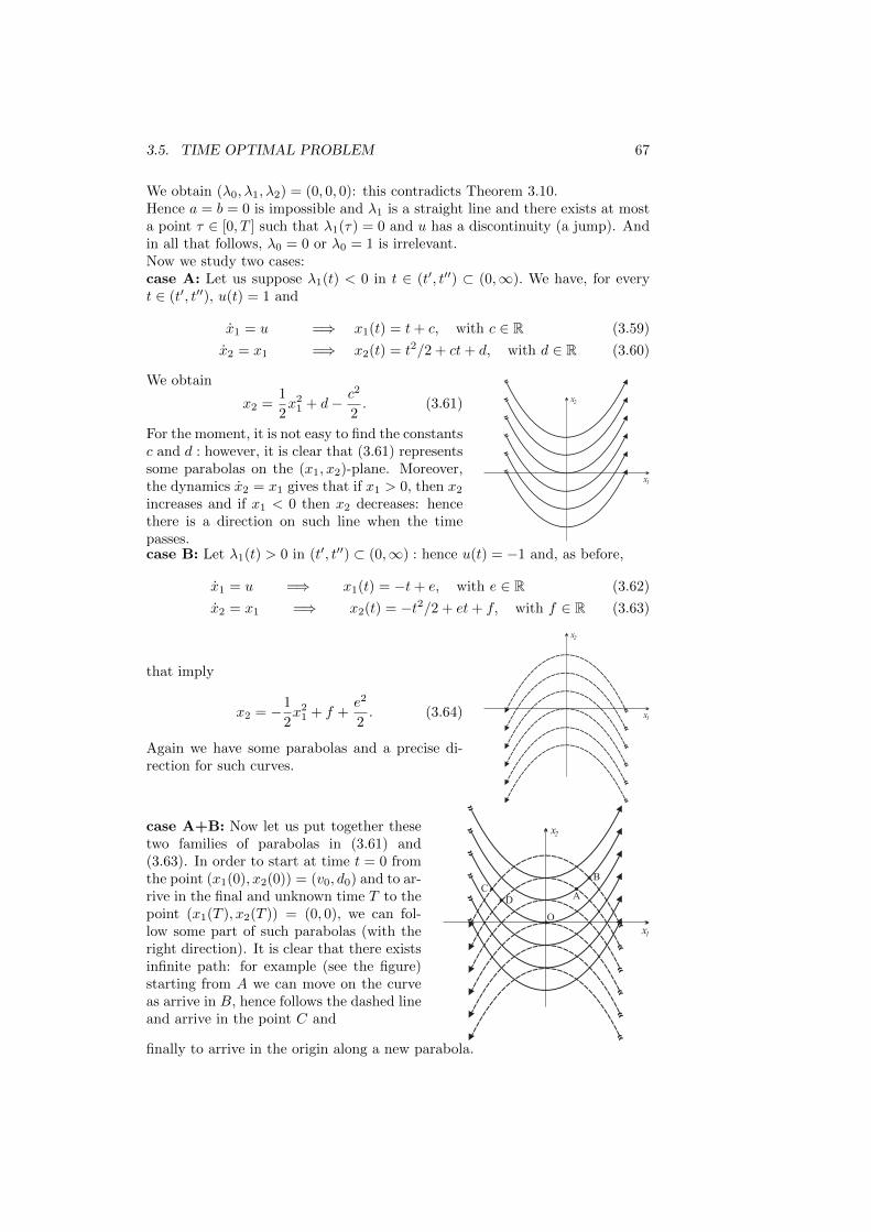
3.5. TIME OPTIMAL PROBLEM 67
We obtain (λ0, λ1, λ2) = (0, 0, 0): this contradicts Theorem 3.10.Hence a = b = 0 is impossible and λ1 is a straight line and there exists at mosta point τ ∈ [0, T ] such that λ1(τ) = 0 and u has a discontinuity (a jump). Andin all that follows, λ0 = 0 or λ0 = 1 is irrelevant.Now we study two cases:case A: Let us suppose λ1(t) < 0 in t ∈ (t′, t′′) ⊂ (0,∞). We have, for everyt ∈ (t′, t′′), u(t) = 1 and
x1 = u =⇒ x1(t) = t+ c, with c ∈ R (3.59)
x2 = x1 =⇒ x2(t) = t2/2 + ct+ d, with d ∈ R (3.60)
We obtain
x2 =1
2x21 + d− c2
2. (3.61)
For the moment, it is not easy to find the constantsc and d : however, it is clear that (3.61) representssome parabolas on the (x1, x2)-plane. Moreover,the dynamics x2 = x1 gives that if x1 > 0, then x2increases and if x1 < 0 then x2 decreases: hencethere is a direction on such line when the timepasses.
x1
x2
case B: Let λ1(t) > 0 in (t′, t′′) ⊂ (0,∞) : hence u(t) = −1 and, as before,
x1 = u =⇒ x1(t) = −t+ e, with e ∈ R (3.62)
x2 = x1 =⇒ x2(t) = −t2/2 + et+ f, with f ∈ R (3.63)
that imply
x2 = −1
2x21 + f +
e2
2. (3.64)
Again we have some parabolas and a precise di-rection for such curves.
x1
x2
case A+B: Now let us put together thesetwo families of parabolas in (3.61) and(3.63). In order to start at time t = 0 fromthe point (x1(0), x2(0)) = (v0, d0) and to ar-rive in the final and unknown time T to thepoint (x1(T ), x2(T )) = (0, 0), we can fol-low some part of such parabolas (with theright direction). It is clear that there existsinfinite path: for example (see the figure)starting from A we can move on the curveas arrive in B, hence follows the dashed lineand arrive in the point C and
x
A
1
x2
O
B
C
D
finally to arrive in the origin along a new parabola.

68 CHAPTER 3. GENERAL PROBLEMS OF OC
We remark that every time we pass froma curve to another curve, the optimal con-trol has a discontinuity point, i.e. u∗ passesfrom +1 to −1 or vice versa. Since we knowthat the optimal control has at most onediscontinuity point, the “red line ADO” inthe figure is the unique candidate to realizethe min, i.e. the minimal time T ∗.
x
A
1
x2
O
D
In order to guarantee that u∗ is really the optimal control with exit time T ∗,we suggest two possibilities:• first we will provide an existence result for this particular type of time optimalproblem called “linear”(see subsection 3.4.1). As we mentioned, the dynamicsin (3.53) is exactly the system in (3.43). For such M and N matrices, we have
G(M,N) = [N,MN ] =
[(0
1
),
(0 1
0 0
)(0
1
)]=
(0 1
1 0
)and
det (M − θI) = θ2.
Since G(M,N) has rank 2, and 0 is the unique eigenvalue of the matrix M,Theorem 3.9 guarantees the existence of the solution of (3.53), for every initialdata (v0, d0).•• Second, we can apply a generic result of the existence of an optimal control(see Theorem 3.8). We know, by the previous construction, that there exists atleast an admissible control u∗ with exit time T ∗; hence it is reasonable to restrictthe original target set S = [0,∞)×(0, 0) to the new set S = [0, T ∗]×(0, 0).Moreover, we have a compact control set [−1, 1] and for the dynamics we havethe bounded condition
‖x‖ =
∥∥∥∥( u
x1
)∥∥∥∥ ≤√1 + x21 ≤ (1 + |x1|) ≤ (1 + ‖x‖);
finally, for every (t, x1, x2) we have that
F(t,x1,x2) = (y1, y2, z) : y1 = u, y2 = x1, z ≥ 1, u ∈ [−1, 1]= [−1, 1]× x1 × [1,∞),
is a convex set. Hence Theorem 3.8 guarantees that the optimal control exists.
In the next example we solve a particular case of this general situation:
Example 3.5.3. Let us consider
minuT
x1 = ux2 = x1x1(0) = 2, x2(0) = 1x1(T ) = x2(T ) = 0|u| ≤ 1

3.5. TIME OPTIMAL PROBLEM 69
Since A = (x1(0), x2(0)) = (α1, α2) = (2, 1), by (3.62) and (3.63) we obtain e = 2 e f = 1.(3.61) gives the curve γ1 with equation
x2 = −x21/2 + 3.
The point D is the intersection of the curve γ2 with equation
x2 = x21/2,
and the curve γ1 : we obtain D = (−√
3, 3/2). We note that starting from A at time t = 0,we arrive in D at time τD : such τD is, by (3.62), τD = 2 +
√3.
We restart from D = (x1(τD), x2(τD)) and arrive, on γ2, to O. By (3.59) we have x1(τD) =τD + c = −
√3 and hence c = −2(1 +
√3). By (3.61) and the equation of γ2, we have
d = c2/2 = 4(2 +√
3). We arrive in the origin at the time T that is, using (3.59) and hencex1(T ) = T − 2(1 +
√3) = 0, T = 2(1 +
√3). Hence
T ∗ = 2(1 +√
3).
The optimal control and the optimal trajectory are (in order to guarantee that we have reallythe optimal control, see the discussions in the previous general case)
u∗(t) =
−1 for t ∈ [0, 2 +
√3],
1 for t ∈ (2 +√
3, 2(1 +√
3)],
x∗1(t) =
−t+ 2 for t ∈ [0, 2 +
√3],
t− 2(1 +√
3) for t ∈ (2 +√
3, 2(1 +√
3)],
x∗2(t) =
−t2/2 + 2t+ 1 for t ∈ [0, 2 +
√3],
t2/2− 2(1 +√
3)t+ 4(2 +√
3) for t ∈ (2 +√
3, 2(1 +√
3)],
t0
u
t
u
D T
1
-1
x
t0 tD T
2
-3
1
1/2
x
t0
tD T
1
3/2
2
4
3.5.2 The Dubin car
The simple car model has three degrees of freedom, the car can be imagined asa rigid body that moves in a plane. The back wheels can only slide and thatis why parallel parking is challenging. If all wheels could be rotated together,parking would be a trivial task. The position of a car can be identified, at everytime t, with the triple (x1, x2, θ) ∈ R2× [0, 2π), where (x1, x2) are the principaldirections and θ is the angle of the car with the x1 axis.Suppose that the car has an initial position (x1(0), x2(0), θ(0)) = (4, 0, π/2) andwe are interested to park the car in the position (0, 0), without constraints onthe final direction of the car, in the shortest time. Clear, the fact that we haveno condition on the final direction simplifies the problem.9
9If we add an assumption on the final direction of the car, as is reasonable if you areparking it, then we have the following Dubin car problem:
minuT
x1 = cos θx2 = sin θθ = ux1(0) = x1,0, x2(0) = x2,0, θ(0) = θ0x1(T ) = 0, x2(T ) = 0, θ(T ) = θ1|u| ≤ 1
The solution is much more complicated and is presented, for example, in [1].

70 CHAPTER 3. GENERAL PROBLEMS OF OC
From the geometry of the model (simplifying some constants to unity, i.e. wethink that the velocity of the car is constant and equal to 1), the followingproblem can be retrieved:
minuT
x1 = cos θx2 = sin θθ = ux1(0) = 4, x2(0) = 0, θ(0) = π/2x1(T ) = 0, x2(T ) = 0|u| ≤ 1
(3.65)
The Hamiltonian is H = λ0 + λ1 cos θ+ λ2 sin θ+ λ3u and the necessary condi-tions of Theorem 3.10 give (note that θ(T ) is free and hence we have a furthertransversality condition on λ3(T ))
u(t) ∈ arg minv∈[−1,1]
λ3(t)v (3.66)
λ1 = − ∂H∂x1
= 0 ⇒ λ1 = c1 (3.67)
λ2 = − ∂H∂x2
= 0 ⇒ λ2 = c2 (3.68)
λ3 = −∂H∂θ
= λ1 sin θ − λ2 cos θ (3.69)
λ3(T ) = 0 (3.70)
λ0 + λ1(T ) cos θ(T ) + λ2(T ) sin θ(T ) + λ3(T )u(T ) = 0 (3.71)
where ci are constants; changing these constants with c1 = α cosβ and c2 =α sinβ, where α ≥ 0 and β are again constants, we obtain by (3.67)–(3.71) that
λ1 = α cosβ, λ2 = α sinβ (3.72)
λ3 = α sin(θ − β) (3.73)
λ0 + α cosβ cos θ(T ) + α sinβ sin θ(T ) = 0 (3.74)
It is easy to see that if α = 0 (i.e. λ1(t) = λ2(t) = 0), then by (3.74) we obtainλ0 = 0; moreover (3.73) and (3.70)) give λ3(t) = 0. This is impossible since(λ0, λ) 6= (0, 0): hence α 6= 0. We note that if (λ0, λ1, λ2, λ3) is a multiplier thatsatisfies all the conditions (3.66)–(3.71), the “new” multiplier (λ0
α ,λ1
α ,λ2
α ,λ3
α )satisfies the same conditions (3.66)–(3.71). In other words, it is possible to put,without loss of generality, α = 1.
First, let us suppose that there exists an interval (a, b) where
λ3(t) > 0, t ∈ (a, b);
(3.66) implies u = −1 in such interval. The dynamics gives
θ(t) = −t+ a+ θ(a), ∀t ∈ (a, b)
and hence
x1(t) = x1(a)− sin(−t+ a+ θ(a)) + sin θ(a)
x2(t) = x2(a) + cos(−t+ a+ θ(a))− cos θ(a)

3.5. TIME OPTIMAL PROBLEM 71
for every t ∈ (a, b). Note that t 7→ (x1(t), x2(t)) describes an arc of circumferenceof radius 1, in a clockwise sense.
Similar calculations give that if there exists an interval (a, b) where
λ3(t) < 0, t ∈ (a, b)
then we obtain u(t) = +1 and
θ(t) = t− a+ θ(a),
x1(t) = x1(a) + sin(t− a+ θ(a))− sin θ(a) (3.75)
x2(t) = x2(a)− cos(t− a+ θ(a)) + cos θ(a) (3.76)
for every t ∈ (a, b). Again t 7→ (x1(t), x2(t)) describes an arc of circumferenceof radius 1, in a counterclockwise sense.
Finally, if we have a situation where
λ3(t) = 0, ∀t ∈ (a, b)
then, λ3(t) = 0 in (a, b): the continuity of θ implies
sin(θ(t)− β) = 0 t ∈ (a, b),
i.e. θ constant in [a, b]. The dynamics gives
x1(t) = x1(a)+(t−a) cos(θ(a)), x2(t) = x2(a)+(t−a) sin(θ(a)) (3.77)
for every t ∈ (a, b).Essentially, in order to construct our optimal strategy we have only three
possibilities:
• we turn on the right with θ = −1, and the car describes an arc of circum-ference of radius 1;
• we turn on the left with θ = 1, and the car describes an arc of circumferenceof radius 1;
• we go straight, i.e. θ = 0.
Now, looking the position of the car, it is reasonable to think that ourstrategy is first to turn on the right and hence to go straight. Hence in [0, τ) weset u(t) = 1 and, as in (3.75)–(3.76) and using the initial conditions, we obtain
θ(t) = t+π
2
x1(t) = 3 + sin(t+
π
2
)= 3 + cos t (3.78)
x2(t) = − cos(t+
π
2
)= sin t
for every t ∈ [0, τ). In [τ, T ] we go straight and hence, as in (3.77) and using thecontinuity of the trajectory for t = τ , we have by (3.78)
θ(t) = τ +π
2
x1(t) = 3 + cos τ − (t− τ) cos(τ +
π
2
)= 3 + cos τ − (t− τ) sin τ
x2(t) = sin τ + (t− τ) sin(τ +
π
2
)= sin τ + (t− τ) cos τ

72 CHAPTER 3. GENERAL PROBLEMS OF OC
for every t ∈ [τ, T ]. Clearly the final condition on the position of the car gives
x1(T ) = 3 + cos τ − (T − τ) sin τ = 0, x2(T ) = sin τ + (T − τ) cos τ = 0.
Solving these system we obtain (using the picture below we deduce that sin τ =+√
8/3)
T ∗ = arccos
(−1
3
)+√
8, τ = arccos
(−1
3
).
Hence
u∗(t) =
1 t ∈ [0, τ ]0 t ∈ (τ, T ∗]
θ∗(t) =
t+ π/2 t ∈ [0, τ ]τ + π/2 t ∈ (τ, T ∗]
x∗1(t) =
3 + cos t t ∈ [0, τ ]8/3− (t− τ)
√8/3 t ∈ (τ, T ∗]
(3.79)
x∗2(t) =
sin t t ∈ [0, τ ]√
8/3− (t− τ)/3 t ∈ (τ, T ∗](3.80)
2
x4
x
13
q(0)
The initial data for the car is (x1(0), x2(0), θ1(0)) = (4, 0, π/2); the final position is
(x1(T∗), x2(T
∗)) = (0, 0) with θ1(T∗) free.
Clear, the previous arguments gives a candidate to be the optimal solution ofthe problem, but it is not a proof of its uniqueness. Indeed, it is possible toconstruct infinite paths using arcs of circumferences of radius 1 and segmentsto connect the point (4,0) and the origin, with continuous θ: such paths areall extremals. However, it is easy to see that in this family of extremal paths,our trajectory (x∗1, x
∗2) in (3.79)-(3.80) is the shortest: since the modulo of the
velocity of the car is constant, such trajectory is the best choice in the familyof the extremals to have a minimal time. We remark that such control u∗ insingular.
Finally, let us show that there exists the optimal control for our problem.We know, by the previous construction, that there exists at least an admissiblecontrol u∗ with exit time T ∗; hence it is reasonable to restrict the original targetset S = [0,∞)× (0, 0) × [0, 2π] to the new set S = [0, T ∗]× (0, 0) × [0, 2π].Moreover, we have a compact control set [−1, 1] and for the dynamics we havethe bounded condition
‖x‖ =
∥∥∥∥∥∥ cos θ
sin θ
u
∥∥∥∥∥∥ ≤√
1 + u2 ≤ 2;

3.6. INFINITE HORIZON PROBLEMS 73
finally, for every (t, x1, x2, θ) fixed we have that
F(t,x1,x2,θ) = (cos θ, sin θ) × [−1, 1]× [1,∞),
is a convex set. Hence Theorem 3.8 guarantees that the optimal control exists.
3.6 Infinite horizon problems
If in the problem (3.4) we consider, with due caution, t1 = ∞, then the firstquestion is the validity of Theorem of Pontryagin 3.1. It is clear that
• with ψ(x(∞)) and x(∞), we have to replace limt→∞
ψ(x(t)) and limt→∞
x(t);
• in general, without other assumptions on f, on the control u∗ and theassociated trajectory x∗ that are candidate to maximize (or minimize)the problem, we are not able to guarantee that the integral∫ ∞
t0
f(t,x∗,u∗) dt
exists and is finite.
In this context and considering the transversality condition iii) of Theorem ofPontryagin, one might expect that
limt→∞
λ∗(t) = 0 (3.81)
would be a natural condition for a infinite horizon problem. The next exampleshows that (3.81) is false:
Example 3.6.1 (The Halkin counterexample). Let us consider the problem
max J(u)
J(u) =
∫ ∞0
(1− x)u dt
x = (1− x)ux(0) = 00 ≤ u ≤ 1
If we integrate the dynamics x + xu = u and taking into account the initial condition, weobtain
x(t) = e−∫ t0 u(s) ds
(∫ t
0u(s)e
∫ s0 u(v) dv ds
)= 1− e−
∫ t0 u(s) ds.
Hence, for every admissible control u the associated trajectory x is such that x(t) ≤ 1. Hence,using the dynamics and the initial condition,
J(u) = limT→∞
∫ T
0(1− x)u dt = lim
T→∞
∫ T
0xdt = lim
T→∞(x(T )− x(0)) ≤ 1.
Hence, every function u such that
∫ ∞0
u(t) dt = ∞ gives J(u) = 1 and hence is optimal.
For example, consider the constant control u0(t) = u0 ∈ (0, 1): it is optimal. Since theHamiltonian is H = (1− x)(1 + λ)u, the PMP implies that
u0 ∈ arg maxv∈[0,1]
(1− x)(1 + λ)v ∀t ≥ 0.
The previous condition gives λ(t) = −1 for every t ≥ 0. Hence such multiplier λ is associated
to the optimal control u0 and limt→∞
λ(t) 6= 0. 4

74 CHAPTER 3. GENERAL PROBLEMS OF OC
Hence let us consider the problem:
maxu∈C
∫ ∞t0
f(t,x,u) dt
x = g(t,x,u)x(t0) = αlimt→∞
xi(t) = βi, for 1 ≤ i ≤ n′
limt→∞
xi(t) ≥ βi, for n′ < i ≤ n′′
limt→∞
xi(t) free for n′′ < i ≤ nC = u : [t0,∞)→ U ⊆ Rk, u admissible
(3.82)
where α and β = (β1, . . . , βn) are fixed in Rn.The problem of the transversality for this problem is treated with many
details in [26] (see Theorem 3.13): here we give only a sufficient condition inthe spirit of the theorem of Mangasarian:
Theorem 3.11. Let us consider the infinite horizon maximum problem (3.82)with f ∈ C1 and g ∈ C1. Let the control set U be convex. Let u∗ be a normalextremal control, x∗ the associated trajectory and λ∗ = (λ∗1, . . . , λ
∗n) the asso-
ciated multiplier, i.e. the tern (x∗,u∗,λ∗) satisfies the PMP and the adjointequation.Suppose that
v) the function (x,u) 7→ H(t,x,u,λ∗(t)) is, for every t ∈ [t0,∞), concave,
vi) for all admissible trajectory x,
limt→∞
λ∗(t) · (x(t)− x∗(t)) ≥ 0. (3.83)
Then u∗ is optimal.
Proof. The first part of the proof coincides with the proof of Theorem 2.3of Mangasarian: hence we obtain that, for every admissible control u withassociated trajectory x we have that (see (2.26))
H(t,x,u,λ∗) ≤ H(t,x∗,u∗,λ∗)− λ∗ · (x− x∗)
and hence, for every that t1 > t0∫ t1
t0
f(t,x,u) dt ≤∫ t1
t0
f(t,x∗,u∗) dt+(λ∗ · (x∗ − x)
∣∣∣t1t0
=
∫ t1
t0
f(t,x∗,u∗) dt+
+λ∗(t1) ·(x∗(t1)− x(t1)
)− λ∗(t0) ·
(x∗(t0)− x(t0)
).
Now, taking into account x∗(t0) = x(t0) = α, the limit for t1 → ∞ of themembers of the previous inequality gives∫ ∞
t0
f(t,x,u) dt ≤∫ ∞t0
f(t,x∗,u∗) dt+ limt1→∞
λ∗(t1) ·(x∗(t1)− x(t1)
). (3.84)

3.6. INFINITE HORIZON PROBLEMS 75
Clearly the transversality condition (3.83) implies that u∗ is optimal.
The transversality condition in (3.83) is not so easy to guarantee, since itrequires to study every admissible trajectory. Suppose that in problem (3.82)we have n′ = n′′ = n, i.e. we have a final condition on the trajectory of the type
limt→∞
x(t) = β, (3.85)
for some fixed β ∈ Rn. It is clear by the final part the previous proof (see (3.84)),that
Remark 3.6. Suppose that in the problem (3.82) we have only a condition ofthe type (3.85). Suppose that there exists a constant c such that
‖λ∗(t)‖ ≤ c, ∀t ≥ τ (3.86)
for some τ, then the transversality condition in (3.83) holds.
See chapter 14 in [8] for further conditions.In the case of infinite horizon problem of Calculus of Variation, recalling
that ∇uf = ∇xf = −λ∗ (see (2.36)), the sufficient condition in (3.83) and in(3.86) become as follows:
Remark 3.7. In the case of infinite horizon problem of Calculus of Variation,the transversality condition in vi) becomes
limt→∞
∇xf(t,x∗(t), x∗(t)) · (x(t)− x∗(t)) ≤ 0, (3.87)
for all admissible trajectory x. Moreover, if the calculs of variation problem hasa final condition on the trajectory of the type (3.85), i.e. limt→∞ x(t) = β withβ fixed, and there exists a constant c such that
‖∇xf(t,x∗(t), x∗(t))‖ ≤ c, ∀t ≥ τ (3.88)
for some τ, then the transversality condition in (3.87) holds.
Finally, it is clear from the proof that
Remark 3.8. If in (3.82) we replace the max with a min, we have to reversethe inequalities in the previous transversality conditions in (3.83) and (3.87).
Example 3.6.2. Let us consider the problemmin
∫ ∞0
e2t(u2 + 3x2) dt
x = ux(0) = 2
It is a calculus of variation problem and in order to guarantee that∫∞0 e2t(u2 + 3x2) dt <∞,
it is clear that we have to require that limt→∞
x(t) = 0. Hence we have to solve the problemmin
∫ ∞0
e2t(x2 + 3x2) dt
x(0) = 2limt→∞
x(t) = 0
The EU gives x+ 2x− 3x = 0 and its general solution is
x(t) = ae−3t + bet,

76 CHAPTER 3. GENERAL PROBLEMS OF OC
for some constants a and b. The conditions on the trajectory give that the unique extremal isthe function x∗(t) = 2e−3t.
Now we note that ∂f∂x
= 2e2tx and hence∣∣∣∣∂f∂x (t, x∗(t), x∗(t))
∣∣∣∣ = |2e2tx∗(t)| = | − 12e−t| ≤ 12, ∀t ≥ 0 : (3.89)
the concavity of the function f = e2t(x2 + 3x2), with respect to the variable x and x, and thetransversality condition (3.88), i.e. (3.89), give that x∗ is optimal.
3.6.1 The model of Ramsey
We show the problem of resource allocation in a infinite time (see [23]): we wantto determine the combination optimal of consumption and savings from currentproduction. Considering a generic economic system that produces a given levelof national product (NP), we must find the fraction of NP that is consumed andwhat is saved: the first generates utility in the current period, while the secondfraction of NP, if invested, will produce a utility in the future.Suppose then that the control variables are the work L = L(t) and the capitalK = K(t). Suppose also that there is only a goods with production function
Q = Q(K(t), L(t)). (3.90)
So the production is independent, directly, by time and hence we are assumingthat there is not progress in the technology. Suppose also that there is nodepreciation of the capital and that the population remains stationary. Theproduction is distributed, at every moment, for consumption C and investments:then
Q = C +K ′. (3.91)
The utility function U = U(C) (social utility index) has not increasing marginalutility η = U ′ : then U ′′ ≤ 0. Moreover we suppose that U has an upper boundwhich we call U .
U
C
U
U
C
U
U
C
U
We note that if U(C)→ U . then η → 0.
We introduce also the disutility function D = D(L) arising from work L, withmarginal disutility decreasing: then D′′ ≥ 0. The net utility is given by U(C)−D(L). The problem of detecting a dynamic consumption that maximizes theutility of current and future generations can formalize as
max(L,C)
∫ ∞0
(U(C)−D(L)) dt. (3.92)
In general the integral in (3.92) does not exist. This is due in part to thefact that there isn’t discount factor, not forgetfulness, but because it is deemed

3.6. INFINITE HORIZON PROBLEMS 77
“ethically indefensible”, for today’s generations who plan, pay the utilities offuture generations. Moreover it is reasonable to expect that over the course oftime the net utility is positive and grows. Hence, we can assume that thereexists a positive B such that
limt→∞
(U(C)−D(L)) = B;
such B is a kind of “ideal situation” (Ramsey called the “Bliss”, happiness).Hence we have to minimize the gap between the net utility and the “happiness”:
min(L,C)
∫ ∞0
[B − U(C) +D(L)
]dt
Taking into account (3.90) and (3.91), we havemin(L,K)
∫ ∞0
[B − U
(Q(K(t), L(t))−K ′(t)
)+D(L(t))
]dt
K(0) = K0
limt→∞
(U(C)−D(L)) = B
(3.93)
where K0 is fixed initial capital, while in general it is considered inappropriatefix an initial condition at work. If we denote by
F = F (L,K,L′,K ′) = B − U(Q(K(t), L(t))−K ′(t)
)+D(L(t)),
we write the equation of Euler with respect the variables L and K :d
dtFL′ = FL
d
dtFK′ = FK
⇒
0 = −ηQL +D′
dη
dt= −ηQK
Since
D′ = ηQL,
the marginal disutility of labor must be equal to the product between themarginal utility of consumption and the marginal product of labor. Moreoverwe have that
dηdt
η= −QK
provides a “good rule” to consumption: the rate of growth of marginal utilityof consumption should be equal, at every moment, to the marginal product ofcapital changing the sign. Also we note that F does not explicitly depend on tand, from (2.38), we have
F −K ′FK′ = c ⇒ B − U(C) +D(L)−K ′η = c, (3.94)
for every t ≥ 0, where c is a constant. Since the net utility tends to B, it isclear that U(C) goes to U and hence η → 0. From (3.94) we have
0 = limt→∞
[B − U(C) +D(L)−K ′η − c] = −c.

78 CHAPTER 3. GENERAL PROBLEMS OF OC
The relations c = 0 and (3.94) give us the optimal path of the investment K∗′,i.e.
K∗′(t) =B − U(C(t)) +D(L(t))
η(t).
This result is known as “the optimal rule of Ramsey”.
Now, if we would like to guarantee that the extremal path (L∗,K∗) is optimal,we study the convexity of the function F :
d2F (L,K,L′,K ′) =
FLL FLK FLL′ FLK′
FKL FKK FKL′ FKK′
FL′L FL′K FL′L′ FL′K′
FK′L FK′K FK′L′ FK′K′
=
−U ′′Q2
L − U ′QLL +D′′ −U ′′QLQK − U ′QKL 0 U ′′QL−U ′′QLQK − U ′QKL −U ′′Q2
K − U ′QKK 0 U ′′QK0 0 0 0
U ′′QL U ′′QK 0 −U ′′
If we consider the quadratic form
h ·(
d2F (L,K,L′,K ′))· hT ,
with h = (hL, hK , hL, hK), we have
h ·(
d2F (L,K,L′,K ′))· hT =
= h2LD′′(L)− (hL, hK) ·
(QLL QLKQLK QKK
)· (hL, hK)TU ′(C) +
−(hL, hK , hK) ·
Q2L QLQK −QL
QLQK Q2K −QK
−QL −QK 1
· (hL, hK , hK)TU ′′(C).
An easy computation shows that the 3× 3 matrix of the previous expression ispositive semidefinite. Moreover, since D′′(L) ≥ 0 and U ′′(C) ≤ 0, if we assumethat U ′(C) ≥ 0 and Q is concave in the variable (L,K), then the extremal path(L∗,K∗) is really a minimum for the problem (3.93).
An example of a concave pro-duction function Q is given bythe Cobb-Douglas Q(L,K) =aL1−bKb, with a > 0 and 0 < b <1. On the eright, we put the func-tion of Cobb-Douglas Q(L,K) =2L4/5K1/5. 0
00
K
5
10
10 15
20
5
30
L10
15

3.7. CURRENT HAMILTONIAN 79
3.7 Current Hamiltonian
In many problems of economic interest, future values of income and expensesare discounted: if r > 0 is the discount rate, we have the problem
J(u) =
∫ t1
t0
e−rtf(t,x,u) dt
x = g(t,x,u)x(t0) = αmaxu∈C
J(u)
(3.95)
where t1 is fixed and finite; in this situation H(t,x,u,λ) = e−rtf(t,x,u) + λ ·g(t,x,u) and the necessary conditions of Pontryagin are
u∗ ∈ arg maxv∈U
(f(t,x∗,v)e−rt + λ∗ · g(t,x∗,v)
)(3.96)
∇xH = e−rt∇xf(t,x∗,u∗) + λ∗ · ∇xg(t,x∗,u∗) = −λ∗
(3.97)
λ∗(t1) = 0. (3.98)
For simplicity and only for few lines, let us consider the case with n = k = 1(i.e. x = x1 = x, u = u1 = u) and with the control set U = R; moreover wesuppose that ∂g
∂u 6= 0 : then (3.96) implies
λ∗ert = −∂f∂u (t, x∗, u∗)∂g∂u (t, x∗, u∗)
.
Hence, from remark 2.11, λ∗(t) gives the marginal value of the state variable attime t discounted (“brought back”) at time t0. It is often convenient to considerthe situation in terms of current values, i.e. of values at time t.Hence, for the generic problem (3.95), let us define the current Hamiltonian Hc
asHc(t,x,u,λc) = f(t,x,u) + λc · g(t,x,u),
where λc is the current multiplier. Clearly we obtain
Hc = ertH (3.99)
λ∗c = ertλ∗. (3.100)
If we consider the derivative with the respect the time in (3.100), we have
λ∗c = rertλ∗ + ertλ
∗
(by (3.97) and (3.100) ) = rλ∗c −∇xf(t,x∗,u∗)− ertλ∗ · ∇xg(t,x∗,u∗)
(by (3.100)) = rλ∗c −∇xf(t,x∗,u∗)− λ∗c · ∇xg(t,x∗,u∗)
= rλ∗c −∇xHc(t,x∗,u∗,λ∗c).
(3.96) and (3.99) imply
u∗(t) ∈ arg maxv∈U
e−rtHc(t,x∗(t),v,λ∗c(t)) = arg maxv∈U
Hc(t,x∗(t),v,λ∗c(t)).
Easily (3.98) becomes λ∗c(t1) = 0. In conclusion
80 CHAPTER 3. GENERAL PROBLEMS OF OC
Remark 3.9. A necessary condition for the problem (3.95) is
u∗ ∈ arg maxv∈U
Hc(t,x∗,v,λ∗c) (3.101)
λ∗c = rλ∗c −∇xH
c(t,x∗,u∗,λ∗c) (3.102)
λ∗c(t1) = 0. (3.103)
We will give an interpretation of the current multiplier in remark 5.7. Clearly(3.99) implies the following;
Remark 3.10 (U = Rk). If in the problem (3.95) we have a control set U = Rk,then in the necessary conditions of remark 3.9 we have to replace (3.101) with
∇uHc(t,x∗,u∗,λ∗c) = 0 (3.104)
Recalling that the transversality condition for the infinite horizon problemis delicate, we have the following:
Remark 3.11 (Infinite horizon problem). If in the problem (3.95) we havet1 =∞, then in the necessary conditions of remark 3.9 we have to delete (3.103).
Example 3.7.1. Let us consider10min
∫ ∞0
e−rt(ax2 + bu2) dt
x = ux(0) = x0 > 0limt→∞
x(t) = 0
(3.105)
where a and b are fixed and positive. The current Hamiltonian is Hc = ax2 + bu2 + λcu.Remark 3.10 gives
∂Hc
∂u= 0 ⇒ 2bu∗ + λ∗c = 0 ⇒ (by (3.108)) λ∗c = −2bx∗ (3.106)
λ∗c = rλ∗c −∂Hc
∂x⇒ λ∗c − rλ∗c + 2ax∗ = 0 (3.107)
∂Hc
∂λc= x∗ ⇒ x∗ = u∗ (3.108)
(3.106) and (3.107) imply
bx∗ − brx∗ − ax∗ = 0 ⇒ x∗(t) = c1e
(br+√b2r2+4ab
)t/(2b)
+ c2e
(br−√b2r2+4ab
)t/(2b)
,
with c1 and c2 constants. The initial condition implies
x∗(t) = c1e
(br+√b2r2+4ab
)t/(2b)
+ (x0 − c1)e
(br−√b2r2+4ab
)t/(2b)
.
Now consider the derivative of the previous expression with respect the time to obtain u∗ :
u∗(t) = c1br +
√b2r2 + 4ab
2be
(br+√b2r2+4ab
)t/(2b)
+
+(x0 − c1)br −
√b2r2 + 4ab
2be
(br−√b2r2+4ab
)t/(2b)
.
It is an easy calculation to see that∫ ∞0
e−rt(a(x∗)2 + b(u∗)2) dt =
∫ ∞0
(Ae
(√b2r2+4ab
)t/b
+Be
(−√b2r2+4ab
)t/b
+ C
)dt,
10In the example 5.7.1 we solve the same problem with dynamic programming.

3.7. CURRENT HAMILTONIAN 81
for A, B and C constants, converges if and only if c1 = 0. We obtain, using (3.100),
λ∗c(t) = x0(√
b2r2 + 4ab− br)e
(br−√b2r2+4ab
)t/(2b)
, (3.109)
λ∗(t) = x0(√
b2r2 + 4ab− br)e−(br+√b2r2+4ab
)t/(2b)
, (3.110)
x∗(t) = x0e
(br−√b2r2+4ab
)t/(2b)
,
u∗(t) = x0br −
√b2r2 + 4ab
2be
(br−√b2r2+4ab
)t/(2b)
.
The Hamiltonian is convex and the multiplier λ∗ is bounded; from Theorem 3.11 and remark3.6 u∗ is the minimum. In the picture at the end of the next example 3.7.2, there is theoptimal tern in a particular case.
Example 3.7.2. Let us consider a modification of the previous example 3.7.1, in the caser = 2, a = 3, b = 1, x0 = 2 :
min
∫ ∞0
e−2t(3x2 + u2) dt
x = ux(0) = 2|u| ≤ 1limt→∞
x(t) = 0
(3.111)
This new problem has some similarities with the previous one: we only give an idea of thesolution and leave to the reader the details. The current Hamiltonian is Hc = 3x2 +u2 +λcu.Remark 3.9 gives
u∗ ∈ arg minv∈[−1,1]
Hc(t, x∗, u∗, λ∗c) ⇒ u∗ ∈ arg minv∈[−1,1]
(v2 + λ∗cv)
⇒ u∗ =
−1 if −λ∗c/2 < −1−λ∗c/2 if −1 ≤ −λ∗c/2 ≤ 11 if 1 < −λ∗c/2
(3.112)
λ∗c = rλ∗c −∂Hc
∂x⇒ λ∗c − 2λ∗c + 6x∗ = 0 (3.113)
∂Hc
∂λc= x∗ ⇒ x∗ = u∗ (3.114)
Let us suppose that for every t ∈ [0,∞) we have −1 ≤ −λ∗c/2 ≤ 1: we obtain (as in example3.7.1)
u∗(t) = −2e−t, x∗(t) = 2e−t, λ∗c(t) = 4e−t, ∀t ∈ [0,∞) :
this contradicts the assumption λ∗c ≤ 2.Hence let us suppose that, for some fixed τ > 0, we have −λ∗c/2 < −1 for every t ∈ [0, τ).
Relations (3.112), (3.113) and (3.114) give
u∗(t) = −1, x∗ = 2− t, λ∗c(t) = Ae2t − 3t+9
2, ∀t ∈ [0, τ). (3.115)
Now let us suppose that for every t ∈ [τ,∞) we have −1 ≤ −λ∗c/2 ≤ 1 : we obtain (as inexample 3.7.1, taking into account that is an infinite horizon problem)
u∗(t) = −c2e−t, x∗(t) = c2e−t, λ∗c(t) = 2c2e
−t, ∀t ∈ [τ,∞). (3.116)
The continuity of the multiplier and of the trajectory in t = τ imply, by (3.115) and (3.116),that
x∗(τ) = 2− τ = c2e−τ ,
λ∗c(τ) = Ae2τ − 3τ +9
2= 2c2e
−τ = 2.
It is an easy calculation to see that
u∗(t) =
−1 if 0 ≤ t < 1−e1−t if t ≥ 1
x∗(t) =
2− t if 0 ≤ t < 1e1−t if t ≥ 1
λ∗c(t) =
12e2t−2 − 3t+ 9
2if 0 ≤ t < 1
2e1−t if t ≥ 1
Since the Hamiltonian is convex and the multiplier λ∗ = λ∗ce−2t is bounded, then u∗ is the
minimum.

82 CHAPTER 3. GENERAL PROBLEMS OF OC
u
1
t0
-1
u =-2e*
-2
-t
u =-e* 1-t
u =-1*
x
t0
1
2
x =e* 1-t
x =2e*-t
x =1*
1
x
t0
2
4
l =4e*-t
c
l =2e*1-t
c
l =e /2-3t+9/2* 2-2t
c
1
In red: the optimal tern of the problem (3.105), in the case r = 2, a = 3, b = 1, x0 = 2.In blue: the optimal tern of the problem (3.111).
3.7.1 A model of optimal consumption with log–utility I
We solve11 the model presented in the example 1.1.5, formulated with (1.6),recalling that here δ > r. Secondly we study a particular case where there is notan excess return, i.e. if where δ is a given discount rate and r > 0 is a given rateto return, then we have δ = r. In both these cases, we consider a logarithmicutility function U(c) = log c.
The case δ > r : we have to study (1.6). The current Hamiltonian is Hc =ln c+ λc(rx− c) and the sufficient condition (3.102) and (3.104) give
λc = (δ − r)λc (3.117)
c(t) ∈ arg maxv≥0
(ln v + λc(rx− v)). (3.118)
Clearly (3.117) gives λc = Ae(δ−r)t for some constant A and the max in (3.118)depends on the such A : more precisely
c(t) =
6 ∃ if λc(t) ≤ 01
λc(t)if λc(t) > 0
Let us suppose12 that A > 0. Hence (3.118) gives c(t) = 1Ae
(r−δ)t. From the
dynamics we obtain x = rx− 1Ae
(r−δ)t and hence
x(t) = e
∫ t
0
r ds
x0 − 1
A
∫ t
0
e(r−δ)se−∫ s
0
r dvds
=
(x0 −
1
Aδ
)ert +
1
Aδe(r−δ)t.
11In subsection 5.7.4 we solve the same problem with the variational approach.12We note that this assumption, taking into account that the multiplier is a shadow price
(see section 5.6), is reasonable since if the initial capital x0 increases, then the value of themax (the total discounted utility) increases.

3.7. CURRENT HAMILTONIAN 83
The condition limt→∞
x(t) = 0 implies A = 1x0δ
: note that this result is consistent
with the assumption on the sign of A. Hence we obtain
c(t) = x0δe(r−δ)t and x(t) = x0e
(r−δ)t.
Since the Hamiltonian is convex and the multiplier λ∗(t) = λ∗c(t)e−δt = 1
x0δe−rt
is bounded, we have the optimal path of consumption.The case δ = r : we suppose that the consumption c is bounded with thespending limit cmax ≥ rx0 and let us remove the assumption lim
t→∞x(t) = ∞ :
then the problem is max
∫ ∞0
e−rt ln cdt
x = rx− cx(0) = x0 > 0x ≥ 00 ≤ c ≤ cmax
Clearly the current Hamiltonian is Hc = ln c + λc(rx − c) and the sufficientcondition (3.102) and (3.104) give
λc = rλc − rλc = 0
c(t) ∈ arg maxv∈[0,cmax]
(ln v + λc(rx− v)). (3.119)
We obtain that λc(t) = λc(0) for every t ≥ 0. We note that
∂Hc
∂c=
1
c− λc(0)
and hence, taking into account (3.119), we obtain: if λc(0) ≤ 0, then Hc in-creases in [0, cmax] and c(t) = cmax; if 0 < 1
λc(0)≤ cmax, then c(t) = 1
λc(0); if
1λc(0)
> cmax, then c(t) = cmax. In all the cases we obtain that c(t) = k is a
constant: hence the dynamics gives
x(t) = e
∫ t
0
r ds
x0 − ∫ t
0
ke−∫ s
0
r dvds
= x0ert − k e
rt − 1
r. (3.120)
We note that k > rx0 implies that limt→∞
x(t) = −∞ : this contradicts the
requirement on the capital x > 0. Hence we consider such constant controlc(t) = k with k ≤ rx0 : we have
maxc(t)=k: k≤rx0
∫ ∞0
e−rt ln cdt =
(maxk≤rx0
ln k
)∫ ∞0
e−rt dt;
hence c∗(t) = rx0 ≤ cmax is the optimal choice in the constant consumptions.Such control c∗ gives a path of the capital constant x∗(t) = x0 and a currentmultiplier λ∗c(t) = 1
rx0.
In order to guarantee that c∗ is the max, we note that the Hamiltonianis concave in the variable (x, c) since the dynamics is linear in the variablesx and c, the running cost is concave in c. To conclude we have to show that

84 CHAPTER 3. GENERAL PROBLEMS OF OC
the transversality condition (3.83) in Theorem 3.11 holds: for every admissibletrajectory x we have x(t) > 0 and hence
−x0 < x(t)− x0 = x(t)− x∗(t).
Taking into account that the multiplier λ∗(t) = λ∗c(t)e−rt = λ∗c(0)e−rt is posi-
tive, we obtain
limt→∞
λ∗(t)(x(t)− x∗(t)) ≥ limt→∞
−λ∗(t)x0 = −1
rlimt→∞
e−rt = 0.
Hence c∗ is really the optimal path of consumption.

Chapter 4
Constrained problems ofOC
The constrained optimal control problems are treated exhaustively in [27] (chap-ter 8, section C); one can also consult [5] and [19].
4.1 The general case
Let f, g : [t0, t1]×Rn+k → R be the running cost and the dynamics respectively;let h = (h1, . . . , hm) : [t0, t1] × Rn+k → Rm be the function for the m equal-ity/inequality constraints and b = (b1, . . . , br) : [t0, t1]×Rn+k → Rr be the func-tion for the r integral equality/inequality constraints; let ψ = (ψ0, ψ1, . . . , ψr) :Rn → Rr+1 be the pay off function and α ∈ Rn the initial point of the trajectory.Let 0 ≤ m′ ≤ m, 0 ≤ r′ ≤ r. We consider the problem
J(u) =
∫ t1
t0
f(t,x,u) dt+ ψ0(x(t1))
x = g(t,x,u)x(t0) = αhj(t,x(t),u(t)) ≥ 0 for 1 ≤ j ≤ m′hj(t,x(t),u(t)) = 0 for m′ + 1 ≤ j ≤ m
Bj(u) =
∫ t1
t0
bj(t,x,u) dt+ ψj(x(t1)) ≥ 0 for 1 ≤ j ≤ r′
Bj(u) =
∫ t1
t0
bj(t,x,u) dt+ ψj(x(t1)) = 0 for r′ + 1 ≤ j ≤ r
maxu∈C
J(u)
C = u : [t0, t1]→ Rk, u admissible for α in t0
(4.1)
where t1 is fixed. We note that we consider a control set U equal to Rk sinceall the possible constraints on the value of u can be write in form of the in-equality constraints hj(t,x,u) ≥ 0 : hence all the restrictions on the controlis incorporated in these type of constraints. We remark that we require thatthe every functions hj depends on the control (see section 4.2 for the casehj(t,x,u) = h(t,x)).
85

86 CHAPTER 4. CONSTRAINED PROBLEMS OF OC
As in the static optimization problem with constraints, there are qualifyingconditions for the equality/inequality constraints that must be true. Here weare not interested in the arguments of the well–known Arrow-Hurwicz-Uzawacondition (see for example [27]); we only recall a sufficient condition so thatthe constraints are qualified. The problem to qualify the equality/inequalityintegral constraints is very different: we will treat this problem in the particularsituation of Calculus of Variation in the next section.
Proposition 4.1. Any one of the following conditions provides the equality/inequalityconstraint qualification in (u∗,x∗), where u∗ is a control and x∗ is the associatedtrajectory:
a) the functions hj(t,x,u) are convex in the variable u, for all x ∈ Rn, t ∈[t0, t1] fixed and j = 1, . . . ,m;
b) the functions hj(t,x,u) are linear in the variable u, for all x ∈ Rn, t ∈[t0, t1] fixed and j = 1, . . . ,m;
c) the functions hj(t,x,u) are concave in the variable u, for all x ∈ Rn, t ∈[t0, t1] fixed and j = 1, . . . ,m; moreover, there exists u′ ∈ U such thath(t,x∗(t),u′) > 0 for every t ∈ [t0, t1];
d) (rank condition) for every t ∈ [t0, t1] fixed, the rank of the m × (k + m)matrix
∂h1(t,x,u)
∂u1. . .
∂h1(t,x,u)
∂ukh1(t,x,u) . . . 0
∂h2(t,x,u)
∂u1. . .
∂h2(t,x,u)
∂uk0 . . . 0
. . . . . . . . . 0 . . . 0∂hm(t,x,u)
∂u1. . .
∂hm(t,x,u)
∂uk0 . . . hm(t,x,u)
(x∗,u∗)
is equal to the number m of the constraints. This condition is equivalentto require that, for every t ∈ [t0, t1] fixed, the rank of the matrix
(∂hE∂u
)=
∂hi1(t,x,u)
∂u1
∂hi1(t,x,u)
∂u2. . .
∂hi1(t,x,u)
∂uk∂hi2(t,x,u)
∂u1
∂hi2(t,x,u)
∂u2. . .
∂hi2(t,x,u)
∂uk. . . . . . . . . . . .
∂hie(t,x,u)
∂u1
∂hie(t,x,u)
∂u2. . .
∂hie(t,x,u)
∂uk
(x∗,u∗)
is equal to the number of effective constraints, where in(∂hE∂u
)we consider
the indices ij ∈ E such that the constraint hij is effective1.
We define the Hamiltonian function H : [t0, t1]× Rn × Rk × R× Rn × Rr → Ras
H(t,x,u, λ0,λ,ν) = λ0f(t,x,u) + λ · g(t,x,u) + ν · b(t,x,u)
1We recall that a constraint hj(t,x,u) ≥ 0 is effective if hj(t,x,u) = 0; hence
E = j : 1 ≤ j ≤ m, hj(t,x,u) = 0.

4.1. THE GENERAL CASE 87
and the Lagrangian function L : [t0, t1]×Rn ×Rk ×R×Rn ×Rr ×Rm → R as
L(t,x,u, λ0,λ,ν,µ) = H(t,x,u, λ0,λ,ν) + µ · h(t,x,u).
We note that the dimensions of the “new multiplier” ν and µ coincide with thenumber of the equality/inequality integral constraints r and with the numberof the equality/inequality constraints m respectively.
We have the following necessary condition (for the proof see theorem 8.C.4in [27]):
Theorem 4.1 (di Hestenes). Let us consider the problem (4.1) with f ∈ C1([t0, t1]×Rn+k), g ∈ C1([t0, t1]× Rn+k), h ∈ C1([t0, t1]× Rn+k), b ∈ C1([t0, t1]× Rn+k)and ψ ∈ C1(Rn).Let u∗ be optimal control and x∗ be the associated trajectory. Let us supposethat the rank condition for the m equality/inequality constraints holds.Then, there exists a multiplier (λ∗0,λ
∗,ν∗,µ∗), with
λ0 constant,
λ∗ = (λ∗1, . . . , λ∗n) : [t0, t1]→ Rn continuous,
ν∗ = (ν∗1 , . . . , ν∗r ) constant,
µ∗ = (µ∗1, . . . , µ∗m) : [t0, t1]→ Rm piecewise continuous (but continuous in
the discontinuity points of u∗),
such that
(λ∗0,λ∗,ν∗,µ∗) 6= (0,0,0,0);
ν∗jBj(u∗) = 0 for j = 1, . . . , r, and ν∗j ≥ 0 for j = 1, . . . , r′;
µ∗jhj(t,x∗,u∗) = 0 for j = 1, . . . , m, and µ∗j ≥ 0 for j = 1, . . . , m′.
Such multiplier satisfies the following conditions:
i) (PMP): for all τ ∈ [t0, t1] we have
H(τ,x∗(τ),u∗(τ), λ∗0,λ∗(τ),ν∗) = max
v∈Uτ,x∗(τ)H(τ,x∗(τ),v, λ∗0,λ
∗(τ),ν∗)
where for (t,x) ∈ [t0, t1]× Rn we define
Ut,x =
v ∈ Rk : hj(t,x,v) ≥ 0 for 1 ≤ j ≤ m′,
hi(t,x,v) = 0 for m′ + 1 ≤ i ≤ m
;
ii) (adjoint equation): in [t0, t1] we have
λ∗ = −∇xL(t,x∗,u∗, λ∗0,λ∗,ν∗,µ∗);
iii) (transversality condition)
λ∗(t1) = ∇xΨ(x∗(t1)),
where Ψ = λ∗0ψ0 +
r∑j=1
ν∗jψj ;

88 CHAPTER 4. CONSTRAINED PROBLEMS OF OC
iv) in [t0, t1] we have
∇uL(t,x∗,u∗, λ∗0,λ∗,ν∗,µ∗) = 0.
A sufficient condition with a proof very similar to the theorem 2.3 of Man-gasarian is the following (for the proof see theorem 8.C.5 in [27])
Theorem 4.2. Let us consider the maximum problem (4.1) with f ∈ C1([t0, t1]×Rn+k), g ∈ C1([t0, t1]× Rn+k), h ∈ C1([t0, t1]× Rn+k), b ∈ C1([t0, t1]× Rn+k)and ψ ∈ C1(Rn).Let u∗ be admissible control in α with associated trajectory x∗ and associatedmultiplier (λ∗0,λ
∗,µ∗,ν∗) that satisfies all the thesis of theorem 4.1.Moreover, let us suppose that
v) f, g, h, b and ψ are concave functions in the variables x and u, for allt ∈ [t0, t1] fixed,
vi) λ∗0 = 1 and for all i, 1 ≤ i ≤ n, t ∈ [t0, t1] we have λ∗i (t) ≥ 0.
Then u∗ is optimal.
We say that the problem (4.1) is autonomous if all the functions involved inthe statement does not depend on t. In this situation we obtain
Remark 4.1. Consider the problem (4.1) and let us suppose that it is au-tonomous. Let u∗ be optimal control and let x∗ and (λ∗0,λ
∗,ν∗,µ∗) be asso-ciated trajectory and multiplier respectively. Then the Hamiltonian is constantalong the optimal path (x∗,u∗, λ∗0,λ
∗), i.e.
t 7→ H(t,x∗(t),u∗(t), λ∗0,λ∗(t)),
is constant in [t0, t1].
Example 4.1.1. Consider2 max
∫ 1
0(v − x) dt
x = ux(0) = 1
8u ∈ [0, 1]v2 ≤ x
The Hamiltonian H and the Lagrangian L are
H = v − x+ λu, L = v − x+ λu+ µ1u+ µ2(1− u) + µ3(x− v2).
We have to satisfy the following necessary conditions:
(u(t), v(t)) ∈ arg max(u,v)∈Ut,x(t)
(v − x+ λu) (4.2)
where Ut,x = (u, v) ∈ [0, 1]× R : v2 ≤ x
λ = −∂L
∂x⇒ λ = 1− µ3 (4.3)
λ(1) = 0 (4.4)
∂L
∂u= 0 ⇒ λ+ µ1 − µ2 = 0 (4.5)
∂L
∂v= 0 ⇒ 1− 2vµ3 = 0 (4.6)
µ1 ≥ 0 (= 0 if u > 0)
µ2 ≥ 0 (= 0 if u < 1)
µ3 ≥ 0 (= 0 if v2 < x)
2This example is proposed in [26].

4.2. PURE STATE CONSTRAINTS 89
Clearly (4.2) implies
(u(t), v(t)) =
(1,√x) if λ > 0
(?,√x) if λ = 0
(0,√x) if λ < 0
If λ > 0, (u(t), v(t)) = (1,√x) implies by the dynamics x = t + A for some constant A.
(4.6) gives µ3 = 12√t+A
and hence, by (4.3),
λ = 1−1
2√t+A
⇒ λ = t−√t+A+B,
for some constant B. µ1 = 0 implies by (4.5) µ2 = t−√t+A+B.
If λ < 0, (u(t), v(t)) = (0,√x) implies by the dynamics x = C for some constant C. (4.6)
gives µ3 = 1
2√C
and hence, by (4.3),
λ = 1−1
2√C
⇒ λ =
(t−
1
2√C
)t+D,
for some constant D. µ2 = 0 implies by (4.5) µ1 = −(t− 1
2√C
)t−D.
Let us suppose that for some τ > 0, we have λ > 0 in [0, τ) : the initial condition x(0) = 18
implies A = 18. If τ > 1, (4.5) gives B = 3
2√2− 1 and hence λ(t) = t −
√t+ 1
8+ 3
2√2− 1 :
note that we obtain λ(0) = 1√2− 1 < 0. Hence τ < 1.
Let us suppose that λ < 0 in (τ, 1] : (4.5) gives D = 12√2− 1. Now the continuity of µ1 in τ
(note that τ is a discontinuity point for u and hence µ is continuous) implies
µ1(τ−) = 0 = −(
1−1
2√C
)τ −
1
2√C
+ 1 = µ1(τ+) ⇒ C =1
4.
The continuity of x and λ in τ give C = 14. and B = − 3
8: in particular we obtain λ = 0 in
[ 18, 1] that contradicts the assumption λ < 0.
Hence let us suppose that λ = 0 in [ 18, 1]; (4.3) gives µ3 = 1 and hence, by (4.6) v = 1
2. The
(PMP) gives v =√x and hence x = 1
4; the dynamics gives u = 0 and finally, by (4.5) and the
continuity of the multiplier in 18
, µ1 = µ2 = 0. Hence we obtain the following situation:
x u v λ µ1 µ2 µ3
in [0, 18
) t+ 18
1√t+ 1
8t−√t+ 1
8+ 3
80 t−
√t+ 1
8+ 3
81
2√t+ 1
8
in [ 18, 1] 1
40 1
20 0 0 1
Let us verify that the rank condition holds:∂h1
∂u
∂h1
∂vh1 0 0
∂h2
∂u
∂h2
∂v0 h2 0
∂h3
∂u
∂h3
∂v0 0 h3
=
1 0 u 0 0
−1 0 0 1− u 0
0 −2v 0 0 x− v2
;
it is to see the for every t ∈ [0, 1] the rank condition holds in the tern (x, u, v) previous obtained.
Finally it is easy to verify that the sufficient conditions of Theorem 4.2 are satisfied. Note
that the problem is autonomous and the have H = v − x+ λu = 14
in [0, 1]. 4
4.2 Pure state constraints
An important and particular situation is the case of the equality/inequalityconstraints where the functions hj in (4.1) do not depend on the control, i.e.constraints of the type
hj(t,x(t),u(t)) = hj(t,x(t)) ≥ 0 (or = 0).

90 CHAPTER 4. CONSTRAINED PROBLEMS OF OC
A simplest example of this situation is x(t) ≥ 0. We remark that with this
type of constraints, the condition of qualification fails since∂hj∂ui
= 0. Hencelet us give the fundamental ideas of this constrained problem, called pure stateconstraints: a very exhaustive exposition is in [26].
We consider the problem
J(u) =
∫ t1
t0
f(t,x,u) dt+ ψ0(x(t1))
x = g(t,x,u)x(t0) = αhj(t,x(t)) ≥ 0 for 1 ≤ j ≤ mmaxu∈C
J(u)
C = u : [t0, t1]→ U, u admissible for α in t0
(4.7)
where t1 ∈ R and U ⊂ Rk are fixed. We introduce the Hamiltonian and theLagrangian functions as usual.
In previously discussed constrained problems, the solution is predicated uponthe continuity of x and λ variables, so that only the control variable u is allowedto jump: here, with pure state constraints, the multiplier λ can also experiencejumps at the junction points where the constraint h(t,x(t)) ≥ 0 turns frominactive to active, or vice versa. The condition v) in the next theorem checks thejump of λ in such discontinuity points τl with respect the effective constraintshj . The following result can be proved (see [26])
Theorem 4.3. Let us consider the problem (4.7) with f ∈ C1([t0, t1]×Rn+k), g ∈C1([t0, t1]× Rn+k), h ∈ C1([t0, t1]× Rn), and ψ0 ∈ C1(Rn).Let u∗ be an admissible control and x∗ be the associated trajectory.We assume that there exist a multiplier (λ∗0,λ
∗,µ∗), with
λ∗0 = 1,
λ∗ = (λ∗1, . . . , λ∗n) : [t0, t1] → Rn is piecewise continuous and piecewise
continuously differentiable with jump discontinuities at τ1, . . . , τN , witht0 < τ1 < . . . < τN ≤ t1,
µ∗ = (µ∗1, . . . , µ∗m) : [t0, t1]→ Rm piecewise continuous,
and
numbers βls, with 1 ≤ l ≤ N, 1 ≤ s ≤ m,
such that the following conditions are satisfied:
i) (PMP): for all τ ∈ [t0, t1] we have
u∗(τ) ∈ arg maxv∈U
H(τ,x∗(τ),v,λ∗(τ))
ii) (adjoint equation): in [t0, t1] we have
λ∗ = −∇xL(t,x∗,u∗,λ∗,µ∗);

4.2. PURE STATE CONSTRAINTS 91
iii) (transversality condition)
λ∗(t1) = ∇xψ0(x∗(t1));
iv) µ∗jhj(t,x∗) = 0 and µ∗j ≥ 0, for j = 1, . . . , m;
v) the numbers βlj are non negative and such that
λ∗i (τ−l )− λ∗i (τ+l ) =
m∑j=1
βlj∂hj(τl,x
∗(τl))
∂xifor 1 ≤ l ≤ N, 1 ≤ i ≤ n;
moreover
v1) βlj = 0 if hj(τl,x∗(τl)) > 0;
v2) βlj = 0 if hj(τl,x∗(τl)) = 0 and ∇xhj(t,x
∗(t)) · g(t,x∗(t),u∗(t)) isdiscontinuous at τl ∈ (t0, t1);
vi) for every τ ∈ [t0, t1], the function
H0(τ,x,λ∗(τ)) = maxv∈U
H(τ,x,v,λ∗(τ))
is concave in x;
vii) h and ψ0 are concave in x.
Then u∗ is optimal.
We think that the following example and the model in subsection 4.2.1 makeclear the assumption of the previous theorem.
Example 4.2.1. Consider3
max
∫ 3
0(4− t)u dt
x = ux(0) = 0x(3) = 3t+ 1− x ≥ 0u ∈ [0, 2]
The Hamiltonian H and the Lagrangian L are
H = (4− t)u+ λu, L = (4− t)u+ λu+ µ(t+ 1− x).
We have to satisfy the following necessary conditions:
u(t) ∈ arg maxv∈[0,2]
(4− t+ λ)v (4.8)
λ = −∂L
∂x⇒ λ = µ (4.9)
µ ≥ 0 (= 0 if t+ 1− x > 0)
The shape of the running cost function f(t, x, u) = (4− t)u suggests to put u = 2 in thefirst part of the interval [0, 3]. Since x(0) = 0, there exists τ1 > 0 such that the constrainth(t, x) = t + 1 − x is inactive in [0, τ1] : in such interval we have µ = 0 and hence (by (4.9))λ = A for some constant A. We suppose that in [0, τ1]
t < 4 +A : (4.10)
3This example is proposed in [26] and it is solved in [9] with a different approach.

92 CHAPTER 4. CONSTRAINED PROBLEMS OF OC
This implies that in our interval, by (4.9), u(t) = 2 and, by the dynamics and the initialcondition x(t) = 2t. With this trajectory we have that
h(t, x(t)) = t+ 1− x(t) = 1− t > 0 ⇔ t < 1;
we obtain τ1 = 1.
In order to maximize, it is a good strategy to increase again f(t, x, u) = (4− t)u with thetrajectory lying in the constraint on the interval [1, τ2], for some τ2 > 1. In order to do that,let us study condition v) of Theorem 4.3 in the point τ1 = 1 :
λ(τ−1 )− λ(τ+1 ) = β1∂h(τ1, x(τ1))
∂x= −β1,
∇xh(t, x(t)) · g(t, x(t), u(t)) = −u(t);
since for t < 1 we know that u(t) = 2 and in order to have h(t, x(t)) = 0 for t ∈ [1, τ2) wehave to require u(t) = 1, the control u has a discontinuity point in t = 1 : condition v2 impliesthat β1 = 0 and λ continuous in τ1. Hence, in order to satisfy (PMP), for t ∈ [1, τ2) we putλ(t) = t− 4; the continuity of such multiplier in t = 1 implies A = −3. Note that the previousassumption (4.10) holds. Moreover, by (4.9), we have µ = 1 in (1, τ2).
Since u ≥ 0 and hence the trajectory is a non de-creasing function, in order to obtain the final condi-tion x(3) = 3, we can consider τ2 = 2 and u = 0 inthe final interval (2, 3]. Clearly, with this choice, wehave a discontinuity for the control u in the pointτ2 = 2 and the same calculations of before give usthat λ is continuous in t = 2. For t ∈ (2, 3], theconstraint is inactive, µ = 0 and again λ = B is aconstant: the continuity of the multiplier in 2 im-plies B = −2.
x
t1 2 3
1
2
3
t+1-x=0 x*
Hence we obtain the following situation:
x u λ µ
in [0, 1) 2t 2 −3 0
in [1, 2] t+ 1 1 t− 4 1
in (2, 3] 3 0 −2 0
Since the function H0 of condition vi) in Theorem 4.3 and the constraint h are linear in
x, then the previous strategy is optimal. 4
4.2.1 Commodity trading
Let us denote by x1(t) and x2(t) respectively the money on hand and the amountof wheat owned at time t. Let x1(0) = m0 > 0 and x2(t) = w0 > 0. At everytime we have the possibility to buy or to sell some wheat: we denote by α(t)our strategy, where α > 0 means buying wheat, and α < 0 means selling. Wesuppose that the price of the wheat is a known function q(t) for all the period[0, T ], with T fixed (clearly q > 0). Let s > 0 be the constant cost of storinga unit of amount of wheat for a unit of time. We assume also that the rate ofselling and buying is bounded; more precisely |α| ≤M, for a given fixed positiveconstant M .

4.2. PURE STATE CONSTRAINTS 93
Our aim is to maximize our holdings at the final time T, namely the sum ofthe cash on hand and the value of the wheat. Hence we have:
max (x1(T ) + q(T )x2(T ))x1 = −sx2 − qαx2 = αx1(0) = m0, x2(0) = w0
x1 ≥ 0, x2 ≥ 0|α| ≤M
Clearly the Hamiltonian H, the Lagrangian L and the pay-off ψ are
H = −λ1(sx2 + qα) + λ2α,
L = −λ1(sx2 + qα) + λ2α+ µ1x1 + µ2x2,
ψ = x1 + qx2.
We have to satisfy the following necessary conditions:
α(t) ∈ arg maxa∈[−M,M ]
[−λ1(t)(sx2(t) + q(t)a) + λ2(t)a]
⇒ α(t) ∈ arg maxa∈[−M,M ]
a(λ2(t)− λ1(t)q(t)) (4.11)
λ1 = − ∂L
∂x1⇒ λ1 = −µ1 (4.12)
λ2 = − ∂L
∂x2⇒ λ2 = sλ1 − µ2 (4.13)
λ1(T ) =∂ψ
∂x1⇒ λ1(T ) = 1 (4.14)
λ2(T ) =∂ψ
∂x2⇒ λ2(T ) = q(T ) (4.15)
µ1 ≥ 0 (= 0 if x1 > 0)
µ2 ≥ 0 (= 0 if x2 > 0)
Now, to solve the model, let us consider a particular situation: we put
T = 2, s = 3, q(t) = t2 + 1, M = 4, m0 = 2 and w0 = 2.
The shape of the function q suggests a strategy. In the first part of our time,the cost of storing the wheat is major then its value: hence it seams like a goodidea to sell the wheal. In the final part of our time the price of the wheal, andhence the value of the wheat owned, increases: hence it is better to buy wheat.Let us follow this intuition in order to solve the problem.
We start with the final part of [0, 2]. It is reasonable to suppose that x1(2)and x2(2) are positive; hence the two constraints h1 = x1 ≥ 0 and h2 = x2 ≥ 0are sure inactive in t = 2. This guarantees that λ = (λ1, λ2) is continuousin such point t = 2. Hence let us suppose that in (τ, 2], for some τ < 2, themultiplier λ is continuous and the constraints are inactive, i.e. µ1 = µ2 = 0.Clearly (4.12)–(4.15) imply
λ1(t) = 1 and λ2(t) = 3t− 1, ∀t ∈ (τ, 2];

94 CHAPTER 4. CONSTRAINED PROBLEMS OF OC
consequently (4.11) implies, for t ∈ (τ, 2]
α(t) ∈ arg maxa∈[4,−4]
a(−t2 + 3t− 2).
Since −t2 + 3t − 2 > 0 in (1, 2), we have α = 4 in (τ, 2], for some τ ∈ (1, 2)(we recall that we have to check that the constraints are inactive in the interval(τ, 2] ).
Let us study the first part of [0, 2]. We note that x1(0) and x2(0) arepositive: hence the two constraints are inactive in t = 2 and λ = (λ1, λ2) iscontinuous in t = 0. Let us suppose that there exists τ ′ > 0 such that for everyt ∈ [0, τ ′) we have
λ2(t)− λ1(t)(t2 + 1) < 0, x1(t) > 0 and x2(t) > 0. (4.16)
Then (4.11) implies α(t) = −4, for t ∈ [0, τ ′). Using the dynamics and the initialconditions on x1 and x2, we obtain
x1(t) =4
3t3 + 6t2 − 2t+ 2 and x2(t) = 2− 4t.
It is easy to see that x1 is positive in [0, 2] and x2 is positive only in [0, 1/2). Itgives us that
• in [0, 1/2], µ1 = 0, λ1 continuous and (by (4.12)) λ1(t) = A,
• in [0, 1/2), µ2 = 0, λ2 continuous and (by (4.13)) λ2(t) = 3At+B,
• the point τ ′ = τ1 = 1/2 can be a jump for the function λ2,
where A and B are constants. Let us study condition v) of the Theorem 4.3 inthe point τ1 = 1/2 :
λ1(τ−1 )− λ1(τ+1 ) = β11
∂h1(τ1,x(τ1))
∂x1+ β1
2
∂h2(τ1,x(τ1))
∂x1= β1
1 ,
λ2(τ−1 )− λ2(τ+1 ) = β11
∂h1(τ1,x(τ1))
∂x2+ β1
2
∂h2(τ1,x(τ1))
∂x2= β1
2 ;
Since h1 is inactive in τ1, we have β12 = 0 that confirms the continuity of λ1 in
τ1. Since
∇xh2(t,x(t)) · g(t,x(t), α(t)) = (0, 1) · (−3x2(t)− q(t)α(t), α(t)) = α(t)
has a discontinuity point in τ1 (for t < τ1 we know that α(t) = −4 and in orderto have x2(t) ≥ 0 for t > τ1 we have to require α(t) ≥ 0), condition v2 impliesthat β1
2 = 0 : hence λ2 is continuous in τ1. The assumption (4.16) becomes
λ2(t)− λ1(t)(t2 + 1) = −At2 + 3At+B −A < 0 for t ∈ [0, 1/2);
moreover, in order to construct the discontinuity for α in t = 1/2 and to guar-antee the PMP (4.11) in t = 1/2, it is necessary to have
λ2(t)− λ1(t)(t2 + 1) = −At2 + 3At+B −A = 0 for t = 1/2.
These last two conditions give
A = −4B and A > 0.

4.2. PURE STATE CONSTRAINTS 95
Now we pass to study the middle part of [0, 2], i.e. the set [1/2, τ ]. Theidea is to connect the trajectory x2 along the constraint h2 = 0 : in order to dothis we put
u(t) = 0, for t ∈ [1/2, τ ]. (4.17)
This clearly gives, in [1/2, τ ],
x2(t) = 0 ⇒ x1(t) = 0 ⇒ x1(t) = 11/3,
since x1(1/2−) = 11/3. In [1/2, τ ], since x1(t) > 0 we have µ1 = 0. By (4.12)and the continuity of λ1 in t = 1/2, we have λ1(t) = A in [1/2, τ ]. From (4.17)and (4.11) we have
0 ∈ arg maxa∈[−4,4]
a(λ2(t)−Aq(t)), for t ∈ [1/2, τ ].
This implies λ2(t) = Aq(t) in [1/2, τ ]. Since λ2 is continuous in t = 1/2 andλ2(1/2−) = 5A/4, we have
λ2(t) = At2 +A.
The previous study of the point τ1 = 1/2 suggests that the multipliers is contin-uous where the control is discontinuous. Now to connect this second part [0, τ ]with the final part [τ, 1], we have to put
A = λ1(τ−) = λ1(τ+) = 1 At2 +A = λ2(τ−) = λ2(τ+) = 3t− 1 :
we obtain A = 1 and τ = 1. The dynamic and the continuity of x1 and x2 inthe point τ = 1 imply
x2(t) = 4t− 4, and x1(t) =4
3t3 − 6t2 + 16t− 23
3, for t ∈ [1, 2].
Note that x1(t) > 0 in this final interval that guarantees µ1 = 0. Finally (4.12)implies µ2 = 2t+ 1 in [1/2, τ ]. Hence we obtain the following situation:
x1 x2 α λ1 λ2 µ1 µ2
in [0, 1/2) 43 t
3 + 6t2 − 2t+ 2 2− 4t −4 1 3t− 14 0 0
in [1/2, 1] 113 0 0 1 t2 + 1 0 2t+ 1
in (1, 2] 43 t
3 − 6t2 + 16t− 233 4t− 4 4 1 3t− 1 0 0
Let us calculate the function H0 of condition vi) in Theorem 4.3:
H0(t, x1, x2, λ∗1, λ∗2) = max
a∈[−M,M ][−λ1(sx2 + qa) + λ2a]
= −3x2 + maxa∈[−4,4]
(−t2 + 3t− 5/4)a if t ∈ [0, 1/2)0 if t ∈ [1/2, 1](−t2 + 3t− 2)a if t ∈ (1, 2]
=
−3x2 − 4(−t2 + 3t− 5/4) if t ∈ [0, 1/2)−3x2 if t ∈ [1/2, 1]−3x2 + 4(−t2 + 3t− 2) if t ∈ (1, 2]
.

96 CHAPTER 4. CONSTRAINED PROBLEMS OF OC
Clearly, for every fixed t, the function H0 is concave in (x1, x2). Since theconstraints h1 and h2 and the pay–off function ψ are linear in x, then theprevious strategy is optimal.
4.3 Isoperimetric problems in CoV
In this section we are interested to specialized the results of the previous sectionto the calculus of variation problems with only equality integral constraints fortrajectory in R (i.e. with n = 1), with fixed initial and final points. This typeof problems is in the big family of the isoperimetric problems of calculus ofvariation. More precisely, let f : [t0, t1]× R2 → R, r ≥ 1, and b = (b1, . . . , br) :[t0, t1]× R2 → R. Let us consider the problem
J(x) =
∫ t1
t0
f(t, x(t), x(t)) dt
x(t0) = αx(t1) = β
Bj(x) =
∫ t1
t0
bj(t, x(t), x(t)) dt− bj = 0 with j = 1, . . . , r
Ottx∈Aiso J(x)
(4.18)
where α, β and bj are fixed constants and Aiso clearly is defined as
Aiso = x ∈ C1([t0, t1]); x(t0) = α, x(t1) = β,Bj(x) = 0 for 1 ≤ j ≤ r.
Since in problem 4.18 u = x, we have H = λ0f(t, x, u) + λu + ν · b : as usual,we obtain
(PMP) ⇒ λ∗0∂f
∂u+ λ∗ + ν∗ · ∂b
∂u= 0
(adjoint equation) ⇒ λ∗0∂f
∂x+ ν∗ · ∂b
∂x= −λ∗.
Considering a derivative with respect to the time in the first relation, and re-placing λ∗ we obtain the EU for a new functions: more precisely we have thatan immediate consequence of theorem 4.1 is the following
Theorem 4.4. Let us consider (4.18) with f and b in C2. Let x∗ ∈ C1 be aminimum (or a maximum).
Then, there exists a constant multiplier (λ∗0,ν∗) 6= 0 such that, in [t0, t1], we
have4d
dtL0x(t, x∗, x∗, λ∗0,ν
∗) = L0x(t, x∗, x∗, λ∗0,ν∗),
where L0 is the generalized Lagrangian function L0 : [t0, t1]×R2×R×Rr → Rdefined as
L0(t, x, x, λ0,ν) = λ0f(t, x, x) + ν · b(t, x, x).
We remark that, in the “language of optimal control”, the function L0 is anHamiltonian; however, in the classical “language of calculus of variation” it iscalled Lagrangian: we prefer this second approach.
4We denote by L0x and by bjx the derivative with respect to x of the functions L0 and bkrespectively.

4.3. ISOPERIMETRIC PROBLEMS IN COV 97
4.3.1 Necessary conditions with regular constraints
As we will see, the study of isoperimetric problems in CoV has some similaritieswith the static optimization problem with equality constraints. Let us startwith the following definition
Definition 4.1. We consider the problem (4.18) with f and b in C2 and letx∗ ∈ C1. We say that the constraints are regular in x∗ if the r functions
d
dtbjx(t, x∗, x∗)− bjx(t, x∗, x∗), j = 1, . . . , r
are linearly independent.
Moreover, we note that the definition of regularity of the constraints is relatedto the choice of the function x∗. The following example clarify the situation
Example 4.3.1. Consider∫ 1
0b1(t, x, x) dt =
∫ 1
0xx2 dt = b1∫ 1
0b2(t, x, x) dt =
∫ 1
0−txdt = b2
Clearly
d
dtb1x(t, x, x)− b1x(t, x, x) = x2 + 2xx,
d
dtb2x(t, x, x)− b2x(t, x, x) = t.
It is easy to see that if we consider the function x∗1 = 0, the constraints are not regular since,for a1 and a2 constants, we have, for every t ∈ [0, 1],
a1
(d
dtb1x(t, x∗1, x
∗1)− b1x(t, x∗1, x
∗1)
)+ a2
(d
dtb2x(t, x∗1, x
∗1)− b2x(t, x∗1, x
∗1)
)= 0
⇔ a2t = 0.
Choosing a1 ∈ R and a2 = 0, the last relation is satisfied. Hence the functions ddtb1x(t, x∗1, x
∗1)−
b1x(t, x∗, x∗1) and ddtb2x(t, x∗1, x
∗1)− b2x(t, x∗, x∗1) are not linearly independent.
A similar computation shows that for the function x∗2 defined by x∗2(t) = t, the constraints
are regular. 4
We remark that in the case of only one constraint (i.e. r = 1), such constraintis regular in x∗ if
d
dtbx(t, x∗, x∗) 6= bx(t, x∗, x∗).
In other words
Remark 4.2. In a isoperimetric problem of calculus of variation with a uniqueconstraint, such constraint is regular in x∗ if x∗ does not satisfy the Euler equa-tion for the function b.
We define the Lagrangian function L : [t0, t1]× R2 × Rr → R by
L(t, x, x,ν) = f(t, x, x) + ν · b(t, x, x). (4.19)
We have the following necessary condition

98 CHAPTER 4. CONSTRAINED PROBLEMS OF OC
Theorem 4.5. Let us consider (4.18) with f and b in C2. Let x∗ ∈ C1 be aminimum (or a maximum). Moreover, let us suppose that the constraints areregular in x∗.
Then, there exists a constant multiplier ν∗ such that, in t ∈ [t0, t1], we have
d
dtLx(t, x∗, x∗,ν∗) = Lx(t, x∗, x∗,ν∗). (4.20)
A function x∗ that satisfies (4.20) (i.e. the EU for the Lagrangian) is calledextremal for the Lagrangian.
It is possible to prove theorem 4.5 as an application of the Dini’s Theorem,as in the static optimization problem with equality constraints: this approachdoes not follow the idea of “variation” of the CoV; a different proof, using avariational approach, is in [7].
Example 4.3.2. We consider
Ott
∫ 1
0x2 dt
x(0) = 0x(1) = 0∫ 1
0xdt =
1
12∫ 1
0txdt =
1
20
First of all, let us study the regularity of the constraints: since b1(t, x, x) = x and b2(t, x, x) =tx, we have
d
dtb1x(t, x∗, x∗)− b1x(t, x∗, x∗) = −1,
d
dtb2x(t, x∗, x∗)− b2x(t, x∗, x∗) = −t.
For every x∗, the functions ddtb1x(t, x∗, x∗)−b1x(t, x∗, x∗) and d
dtb2x(t, x∗, x∗)−b2x(t, x∗, x∗)
are linearly independent since
α1(−1) + α2(−t) = 0, ∀t ∈ [0, 1] ⇔ α1 = α2 = 0.
Hence the constraints are regular for every x∗.The Lagrangian is L = x2 + ν1x + ν2tx; the EU for L is 2x = ν1 + ν2t and the general
solution is
x∗(t) = at+ b+ν1
4t2 +
ν2
12t3,
with a, b ∈ R. The initial condition and the final condition on the trajectory, and the twoconstraints give
x(0) = 0 ⇒ b = 0
x(1) = 0 ⇒ a+ b+ν1
4+ν2
12= 0∫ 1
0xdt =
1
12⇒
∫ 1
0(at+ b+ ν1t
2/4 + ν2t3/12) dt =
= a/2 + b+ ν1/12 + ν2/48 = 1/12∫ 1
0txdt =
1
20⇒
∫ 1
0(at2 + bt+ ν1t
3/4 + ν2t4/12) dt =
= a/3 + b/2 + ν1/16 + ν2/60 = 1/20.
Hence a = b = 0, ν1 = 4 and ν2 = −12. The unique extremal for the Lagrangian is thefunction x∗ = t2 − t3.
Let us show that x∗ is really the minimum of the problem. We want to prove that forevery function x = x∗+h, that satisfies the initial and the final conditions and the two integral

4.3. ISOPERIMETRIC PROBLEMS IN COV 99
constraints, we have J(x∗) ≤ J(x), where J(x) =∫ 10 x
2 dt. Let x = x∗ + h : hence
x(0) = x∗(0) + h(0) ⇒ h(0) = 0 (4.21)
x(1) = x∗(1) + h(1) ⇒ h(1) = 0 (4.22)∫ 1
0xdt =
∫ 1
0(h+ x∗) dt =
1
12⇒
∫ 1
0hdt = 0 (4.23)∫ 1
0txdt =
∫ 1
0t(x∗ + h) dt =
1
20⇒
∫ 1
0thdt = 0. (4.24)
The four previous conditions give
J(x) =
∫ 1
0(x∗ + h)2 dt
=
∫ 1
0(x∗
2+ 2x∗h+ h2) dt
=
∫ 1
0(x∗
2+ 2(2t− 3t2)h+ h2) dt
(by part) =
∫ 1
0(x∗
2+ h2) dt+ 2
((2t− 3t2)h(t)
]10
− 2
∫ 1
0(2− 6t)h dt
(by (4.21) e la (4.22)) =
∫ 1
0(x∗
2+ h2) dt− 4
∫ 1
0h dt+ 12
∫ 1
0thdt
(by (4.23) e la (4.24)) =
∫ 1
0(x∗
2+ h2) dt
≥∫ 1
0x∗
2dt
= J(x∗).
Hence x∗ is a minimum. 4
In this note we are not interested to study the sufficient conditions for theproblem (4.18) (see for example [7]).
4.3.2 The multiplier ν as shadow price
We consider the problem (4.18); let x∗ be a minimum in C2 and let us supposethat the r integral constraints are regular in x∗. Theorem 4.5 guarantees thatthere exists a constant multiplier ν∗ = (ν∗1 , . . . , ν
∗r ) such that EU holds for the
Lagrangian L = f +ν∗ · b in x∗. Let us show an interpretation of the role of thismultiplier ν∗. If we define
J(x) =
∫ t1
t0
f(t, x, x) dt,
clearly J(x∗) is the minimum value for the problem (4.18). Since x∗ satisfy theconstraints we have
r∑j=1
ν∗j
(∫ t1
t0
bj(t, x∗, x∗) dt− bj
)= 0.
Hence
J(x∗) =
∫ t1
t0
f(t, x∗, x∗) dt+
r∑j=1
ν∗j
∫ t1
t0
bj(t, x∗, x∗) dt−
r∑j=1
ν∗j bj
=
∫ t1
t0
L(t, x∗, x∗,ν∗) dt−r∑j=1
ν∗j bj (4.25)

100 CHAPTER 4. CONSTRAINED PROBLEMS OF OC
Our aim is to study the “variation” of the minimum value J(x∗) of the problemwhen we consider a “variation”of the value bk of the k–th constraints; takinginto account (4.25), such “variation” is
∂J(x∗)
∂bk=
∫ t1
t0
(Lx(t, x∗, x∗,ν∗)
∂x∗
∂bk+ Lx(t, x∗, x∗,ν∗)
∂x∗
∂bk
)dt− ν∗k
(by part) =
∫ t1
t0
(Lx(t, x∗, x∗,ν∗)− d
dtLx(t, x∗, x∗,ν∗)
)∂x∗
∂bkdt+
+
(Lx(t, x∗, x∗,ν∗)
∂x∗
∂bk
]t1t0
− ν∗k . (4.26)
Since we have x(t0) = x∗(t0) = α, clearly ∂x∗
∂bk(t0) = 0; a similar argument
implies ∂x∗
∂bk(t1) = 0. By (4.26) and since x∗ is extremal for the Lagrangian, we
have
∂J(x∗)
∂bk=
∫ t1
t0
(Lx(t, x∗, x∗,ν∗)− d
dtLx(t, x∗, x∗,ν∗)
)∂x∗
∂bkdt− ν∗k
= −ν∗k .
Finally∂J(x∗)
∂bk= −ν∗k ,
and ν∗k measures the sensitivity of the optimal value of the problem with respectto a variation of the k-th integral constraints; this is the notion of shadow price.
4.3.3 The foundation of Cartagena
Let us consider the problem (1.2)
max
∫ 1
0
x dt
x(0) = 0x(1) = 0∫ 1
0
√1 + x2 dt = A > 1
and, for symmetry, let us check solution with x(t) ≥ 0. For the function b(t, x, x) =√1 + x2 of the integral constraint we have
bx −d
dtbx = 0 ⇒ x√
1 + x2= d ⇒ x(t) = ±t
√d2
1− d2+ e,
with d, e ∈ R and d 6= ±1. Since the unique function that satisfies the previousrelation and the conditions x(0) = x(1) = 0 is the null function, the constraintis regular since A > 1.The Lagrangian is L = x+ν
√1 + x2 : since Lx = 1, its Euler equation dLx
dt = Lxis Lx + c = t, i.e.
νx√1 + x2
= t− c.

4.3. ISOPERIMETRIC PROBLEMS IN COV 101
Solving for x we obtain
x(t) =t− c√
ν2 − (t− c)2
and hence
x(t) = −√ν2 − (t− c)2 + k ⇒ (x(t)− k)2 + (t− c)2 = ν2.
This solution is a circle and the constants k, c and ν are found using the twoendpoint conditions and the integral constraint. We are not interested to discussthe sufficient conditions.
4.3.4 The Hotelling model of socially optimal extraction
One of the assumptions implicit in the classical theory of production is that allinputs are inexhaustible: in reality this is often not true. The model of Hotelling(see [16], [17]) arises to the problem of considering a dynamic of consumptionof a good whose production is linked to a finite resource. The notion of “thesocial value” of an exhaustible resource is used for judging the desirability ofany extraction pattern of the resource. If we denote by Q(t), with Q(t) ≥ 0, thequantity of extraction of the resource, since it is exhaustible we have∫ ∞
0
Qdt = S0,
with S0 > 0 fixed. The cost to extract a quantity Q of such resource is C =C(Q).The gross social value G of amarginal unit of output of ex-traction of the resource is mea-sured by the price P which so-ciety is willing to pay for suchparticular unit of output. Ifthe price of the resource P isnegatively related to the quan-tity demanded, then the grosssocial value G(Q0) of an out-put Q0 is measured by the yel-low area under the curve, i.e.
P
0 QQ
P=P(Q)
G(Q )0
G(Q0) =
∫ Q0
0
P (Q) dQ.
Hence to find the net social value, we subtract from the gross social value thetotal cost of extraction C(Q0). Hence, the net social value is given by
N(Q) =
∫ Q
0
P (x) dx− C(Q).
We suppose that P is continuous. The problem is to find an optimal path of

102 CHAPTER 4. CONSTRAINED PROBLEMS OF OC
extraction Q(t), the solution ofmaxQ
∫ ∞0
N(Q)e−rt dt
Q(0) = Q0 < S0 Q0 ≥ 0∫ ∞0
Qdt = S0
(4.27)
Clearly r > 0 is a rate of discount.First of all, let us note that the constraint is regular for every function:
indeed, b = b(t, Q,Q′) = Q implies
d
dtbQ′ 6= bQ ⇔ 0 6= 1.
We set the Lagrangian L(t, Q,Q′, ν) = N(Q)e−rt+νQ. The continuity of P andthe fundamental theorem of integral calculus give
d
dtLQ′ = LQ ⇒ P (Q)− C ′(Q) = −νert. (4.28)
Hence (P (Q)− C ′(Q)
)e−rt = c,
with c constant. Along the optimal extraction path, the present differenceP (Q)− C ′(Q) has a uniform value for at every time: this relation is called the“social optimal condition”.
Consider the particular case of n firms of small size compared to themarket and therefore are not able to influence the price. Let P (t) = P0 be theprice of the resource, let Qi be the rate of extraction of the i-th firm and let Sibe the quantity of resource available for the i-th firm. The problem of the i-thfirm is to maximize
max
∫ ∞0
Ni(Qi)e−rt dt
Qi(0) = Q0i < Si Q0
i ≥ 0∫ ∞0
Qi dt = Si
where
Ni(Qi) =
∫ Qi
0
P0 dx− Ci(Qi) = QiP0 − Ci(Qi).
EU for the Lagrangian gives
P0 − C ′i(Qi) = −νert.
This optimality condition is obtained under conditions of pure competition, isperfectly consistent with the social optimal condition (4.28).
However, if we consider the case of a monopoly system in which thecompany has the power to influence the market price, we define R = R(Q) theinput of the monopolist for the quantity Q of resource. The problem of themonopolist is to maximize (4.27), where
N(Q) = R(Q)− C(Q).

4.3. ISOPERIMETRIC PROBLEMS IN COV 103
EU for the Lagrangian gives
R′(Q)− C ′(Q) = −νert;
this is very different from the extraction rule of the social optimal condition:here, the difference between the marginal inputs and the marginal costs growsat a rate r.

104 CHAPTER 4. CONSTRAINED PROBLEMS OF OC

Chapter 5
OC with dynamicprogramming
5.1 The value function: necessary conditions
Let f : [t0, t1]×Rn+k → R, g : [t0, t1]×Rn+k → R and ψ : Rn → R continuousfunctions and α ∈ Rn be fixed. We consider the optimal control
J(u) =
∫ t1
t0
f(t,x,u) dt+ ψ(x(t1))
x = g(t,x,u)x(t0) = αmax
u∈Ct0,αJ(u)
(5.1)
where t0 and t1 are fixed. We recall (see subsection 1.2.1) that Ct0,α denotesthe class of admissible control for α at time t0, i.e. the set of all such controlsu : [t0, t1]→ U that have a unique associated trajectory defined on [t0, t1] withx(t0) = α.We define the value function V : [t0, t1]× Rn → [−∞,∞] for the problem (5.1)as1
V (τ, ξ) =
supu∈Cτ,ξ
(∫ t1
τ
f(t,x,u) dt+ ψ(x(t1))
)if Cτ,ξ 6= ∅;
−∞ if Cτ,ξ = ∅.(5.2)
Clearly, in (5.2), x is the trajectory associated to the control u ∈ Cτ,ξ. The ideaof Bellman [6] and of dynamic programming is to study the properties of suchvalue function. Let us consider (τ, ξ) ∈ [t0, t1]× Rn and the problem
J(u) =
∫ t1
τ
f(t,x,u) dt+ ψ(x(t1))
x = g(t,x,u)x(τ) = ξmaxu∈Cτ,ξ
J(u)
(5.3)
1If in the problem (5.1) we replace the max with a min, in definition (5.2) clearly we haveto replace sup and −∞ with inf and +∞ respectively. In subsection 5.5.2 and in example5.5.4 we will see a min-problem with a value function that admits the value ∞.
105

106 CHAPTER 5. OC WITH DYNAMIC PROGRAMMING
Remark 5.1. If there exists the optimal control u∗τ,ξ for (5.3), then
V (τ, ξ) =
∫ t1
τ
f(t,x∗τ,ξ,u∗τ,ξ) dt+ ψ(x∗τ,ξ(t1)),
where x∗τ,ξ denotes the trajectory associated to u∗τ,ξ.
Example 5.1.1. Let us consider the problemmin
∫ 2
0(u2 + x2) dt
x = x+ ux(0) = 1u ≥ 0
(5.4)
In the example 2.7.1, we have found that, for every (τ, ξ) ∈ [0, 2]× (0,∞) fixed, the problemmin
∫ 2
τ(u2 + x2) dt
x = x+ ux(τ) = ξu ≥ 0
has the optimal tern, see (2.94),
(u∗τ,ξ, x∗τ,ξ, λ
∗τ,ξ) = (0, ξet−τ , ξ(e4−t−τ − et−τ )).
Moreover, the value function V : [0, 2]× [0,∞)→ R for the problem (5.4) is, as in (2.95),
V (τ, ξ) =
∫ 2
0((u∗τ,ξ)
2 + (x∗τ,ξ)2) dt =
ξ2
2(e4−2τ − 1).
4
5.1.1 The final condition on V : an first necessary condi-tion
Consider the problem (5.1) and its value function V. In the particular case ofτ = t1, from the definition (5.2) we have
V (t1, ξ) = supu∈Ct1,ξ
(∫ t1
t1
f(t,x,u) dt+ ψ(x(t1))
)= ψ(ξ).
Hence we have
Remark 5.2.V (t1,x) = ψ(x), for every x ∈ Rn. (5.5)
The condition (5.5) is called the final condition on the value function: clearly,it is a necessary condition for a function V : [t0, t1]× Rn → [−∞,∞] to be thevalue function for the problem (5.1).
If in the problem (5.1) we add a final condition on the trajectory, i.e. x(t1) =β with β ∈ Rn fixed, then the final condition on the value function is
V (t1,β) = ψ(β).
We will see in section 5.4 the condition for the value function when the trajectoryhas a more general condition at the final time.

5.1. THE VALUE FUNCTION: NECESSARY CONDITIONS 107
5.1.2 Bellman’s Principle of optimality
Theorem 5.1 (Bellman’s Principle of optimality). The second part of an opti-mal trajectory is optimal.
More precisely: let us consider the problem (5.1) and let u∗t0,α and x∗t0,α bethe optimal control and the optimal trajectory respectively. Let us consider theproblem (5.3) with (τ, ξ) such that x∗t0,α(τ) = ξ. Let u∗τ,ξ be the optimal controlfor (5.3). Then
u∗t0,α = u∗τ,ξ, in [τ, t1]
and, consequently, x∗t0,α = x∗τ,ξ in [τ, t1].
Proof. Let u∗ be the optimal control for the problem (5.1) and τ ∈ [t0, t1] :we prove that the optimal control u ∈ Cτ,x∗(τ), defined as the restriction ofu∗ on the interval [τ, t1], is optimal for the problem (5.3) with ξ = x∗(τ). Bycontradiction, let us suppose that there exists u] ∈ Cτ,x∗(τ), u] 6= u, optimalfor the problem (5.3) with initial data ξ = x∗(τ) and such that∫ t1
τ
f(t, x, u) dt+ ψ(x(t1)) <
∫ t1
τ
f(t,x],u]) dt+ ψ(x](t1)), (5.6)
where x and x] are the trajectories associated to u and u] respectively. Weconsider the control u defined by
u(t) =
u∗(t) for t0 ≤ t < τ,u](t) for τ ≤ t ≤ t1
(5.7)
and x be the corresponding trajectory.
t
t0
u
t
u*
t1
u
u*
t
t0
x
t
x
t1
a
x*
x*( )t
Clearly u ∈ Ct0,α; hence
V (t0,α) =
∫ t1
t0
f(t,x∗,u∗) dt+ ψ(x∗(t1))
=
∫ τ
t0
f(t,x∗,u∗) dt+
∫ t1
τ
f(t,x∗,u∗) dt+ ψ(x∗(t1))
=
∫ τ
t0
f(t,x∗,u∗) dt+
∫ t1
τ
f(t, x, u) dt+ ψ(x(t1))
(by 5.6) <
∫ τ
t0
f(t,x∗,u∗) dt+
∫ t1
τ
f(t,x],u]) dt+ ψ(x](t1))
(by 5.7) =
∫ t1
t0
f(t,x,u) dt+ ψ(x(t1))
108 CHAPTER 5. OC WITH DYNAMIC PROGRAMMING
that is absurd for the definition of value function. Hence such u] does not exist.
5.2 The Bellman-Hamilton-Jacobi equation
5.2.1 Necessary condition of optimality
The Bellman’s Principle of optimality plays a fundamental role in the proof ofthis crucial property of the value function.
Theorem 5.2. Let us consider the problem (5.1) with f and g continuous andlet us suppose that for every (τ, ξ) ∈ [t0, t1]×Rn there exists the optimal controlu∗τ,ξ for the problem (5.3). Let V be the value function for the problem (5.1)and let V be differentiable. Then, for every (t,x) ∈ [t0, t1]× Rn, we have
∂V
∂t(t,x) + max
v∈U
(f(t,x,v) +∇xV (t,x) · g(t,x,v)
)= 0. (5.8)
The equation (5.8) is called Bellman-Hamilton-Jacobi equation (shortly BHJequation). Clearly (5.8) is a necessary condition for a generic function V tobe the value function for the problem (5.1). The main difficulty of dynamicprogramming is that such equation in general is a Partial Differential Equation(shortly PDE). One of the fundamental property of dynamic programming isthat it is possible to generalize such approach to a stochastic context.
Proof. Let (τ, ξ) ∈ [t0, t1]×Rn be fixed. For the assumptions, there exists theoptimal control u∗τ,ξ for the problem (5.3); we drop to the notation “τ, ξ” andwe set u∗ = u∗τ,ξ. For the Remark 5.1 and for every h > 0 we have
V (τ, ξ) =
∫ t1
τ
f(t,x∗,u∗) dt+ ψ(x∗(t1))
=
∫ τ+h
τ
f(t,x∗,u∗) dt+
∫ t1
τ+h
f(t,x∗,u∗) dt+ ψ(x∗(t1)) (5.9)
where x∗ is the trajectory associated to u∗ with initial point (τ, ξ).For the Bellman’s Principle of optimality (theorem 5.1), the problem (5.3) withinitial point (τ + h,x∗(τ + h)) has as optimal control the function u∗ restrictedto the interval [τ + h, t1]; hence
V (τ + h,x∗(τ + h)) =
∫ t1
τ+h
f(t,x∗,u∗) dt+ ψ(x∗(t1)). (5.10)
Equation (5.9), for (5.10), now is
V (τ, ξ) =
∫ τ+h
τ
f(t,x∗,u∗) dt+ V (τ + h,x∗(τ + h)). (5.11)
Now, let us prove that
maxu∈Cτ,ξ
(∫ τ+h
τ
f(t,x,u) dt+ V (τ + h,x(τ + h))
)=
∫ τ+h
τ
f(t,x∗,u∗) dt+ V (τ + h,x∗(τ + h)) : (5.12)

5.2. THE BELLMAN-HAMILTON-JACOBI EQUATION 109
by contradiction let us suppose that there exists a control u ∈ Cτ,ξ (with asso-ciated trajectory x) such that∫ τ+h
τ
f(t, x, u) dt+ V (τ + h, x(τ + h)) >∫ τ+h
τ
f(t,x∗,u∗) dt+ V (τ + h,x∗(τ + h)), (5.13)
taking into account that there exists an optimal control u∗τ+h,x(τ+h) for the
problem (5.3) with initial point (τ + h, x(τ + h)), then the function u], definedby
u](t) =
u(t) for τ ≤ t < τ + h,u∗τ+h,x(τ+h)(t) for τ + h ≤ t ≤ t1
,
is in Cτ,ξ with associated trajectory x]. Hence (5.11) and (5.13) give∫ t1
τ
f(t,x],u]) dt+ ψ(x](t1)) =
=
∫ τ+h
τ
f(t, x, u) dt+
∫ t1
τ+h
f(t,x∗τ+h,x(τ+h),u∗τ+h,x(τ+h)) dt+ ψ(x∗τ+h,x(τ+h)(t1))
>
∫ τ+h
τ
f(t,x∗,u∗) dt+ V (τ + h,x∗(τ + h))
= V (τ, ξ)
that contradicts the definition of value function. Hence (5.12) holds and, by(5.11), we obtain
V (τ, ξ) = maxu∈Cτ,ξ
(∫ τ+h
τ
f(t,x,u) dt+ V (τ + h,x(τ + h))
). (5.14)
Since V is differentiable, for h sufficiently small,
V (τ + h,x(τ + h)) = V (τ,x(τ)) +∂V
∂t(τ,x(τ))
(τ + h− τ
)+
+∇xV (τ,x(τ)) ·(x(τ + h)− x(τ)
)+ o(h)
= V (τ, ξ) +∂V
∂t(τ, ξ)h+∇xV (τ, ξ) ·
(x(τ + h)− ξ
)+ o(h),
since x(τ) = ξ. Then (5.14) and the previous relation give
maxu∈Cτ,ξ
(∫ τ+h
τ
f(t,x,u) dt+∂V
∂t(τ, ξ)h+∇xV (τ, ξ) ·
(x(τ + h)− ξ
)+ o(h)
)= 0.
If we divide the two members of the previous relation for h > 0 and we considerthe limit for h→ 0+, we obtain
limh→0+
maxu∈Cτ,ξ
( 1
h
∫ τ+h
τ
f(t,x,u) dt+∂V
∂t(τ, ξ) +
+∇xV (τ, ξ) · x(τ + h)− ξ
h+ o(1)
)= 0. (5.15)

110 CHAPTER 5. OC WITH DYNAMIC PROGRAMMING
Now, we note that for a given fixed u ∈ Cτ,ξ we have that in (5.14)∫ τ+h
τ
f(t,x,u) dt+ V (τ + h,x(τ + h)) (5.16)
depends only on the value of u in the set [τ, τ + h] : in fact, given (τ, ξ) and u,we construct x in [τ, τ + h] using the dynamics and hence the value of functionV in (τ + h,x(τ + h)). Hence, for h→ 0+, we have that (5.16) depends only onthe set of the values that u can assume in the point τ, i.e. in the control set U.
Now let us suppose that u is continuous in a neighborhood I of the point τ .Hence the function t 7→ f(t,x(t),u(t)) is continuous in [τ, τ + h], for h small:hence, for the mean value theorem2, we have
inft∈[τ,τ+h]
f(t,x(t),u(t)) ≤ 1
h
∫ τ+h
τ
f(t,x,u) dt ≤ supt∈[τ,τ+h]
f(t,x(t),u(t))
Hence, for the continuity in [τ, τ + h],
limh→0+
1
h
∫ τ+h
τ
f(t,x,u) dt = limt→τ+
f(t,x(t),u(t)) = f(t,x(τ),u(τ)). (5.17)
Now, since t 7→ g(t,x(t),u(t)) is continuous in I, we have x ∈ C1(I) and hence
limh→0+
x(τ + h)− ξ
h= x(τ). (5.18)
If u is not continuous in a neighborhood of τ , i.e. u is only measurable andadmissible, we have only tedious calculations, using the previous ideas, but noreally problems: hence we omit this part of the proof.
Equation (5.15), using (5.17) and (5.18), gives
maxv∈U
(f(τ,x(τ),v) +
∂V
∂t(τ, ξ) +∇xV (τ, ξ) · x(τ)
)= 0. (5.19)
Using the dynamics, the initial condition x(τ) = ξ and remarking that ∂V∂x (τ, ξ)
does not depend on v, we obtain easily (5.8).
Let us consider the problem (5.1); we define the Hamiltonian of DynamicProgramming HDP : [t0, t1]× R2n → (−∞,+∞] defined by
HDP (t,x,p) = maxv∈U
(f(t,x,v) + p · g(t,x,v)
)(5.20)
2We recall that if φ : [a, b]→ R is integrable in [a, b], then
inft∈[a,b]
φ(t) ≤1
b− a
∫ b
aφ(s) ds ≤ sup
t∈[a,b]φ(t);
moreover, if φ is continuous in [a, b], then there exists c ∈ [a, b] such that∫ b
aφ(s) ds = φ(c)(b− a).

5.2. THE BELLMAN-HAMILTON-JACOBI EQUATION 111
It is clear that, in the assumption of Theorem 5.2, the value function solves thesystem
∂V
∂t(t,x) +HDP (t,x,∇xV (t,x)) = 0 for (t,x) ∈ [t0, t1]× Rn
V (t1,x) = ψ(x) for x ∈ Rn(5.21)
It is clear that the previous result in Theorem 5.2 leads naturally to thequestion “when the value function V (τ, ξ) is differentiable”. We will give anidea with Theorem 5.4.
5.2.2 Sufficient condition of optimality
At this point the question is to suggest sufficient conditions such that a functionW : [t0, t1]×Rn → R, that satisfies the Bellman-Hamilton-Jacobi equation (5.8)and the final condition (5.5), is really the value function for the problem (5.1).Moreover, we hope that the value function gives us some information about theoptimal control. This is the content of the next result.
Theorem 5.3. Let us consider the problem (5.1). Let W : [t0, t1]×Rn → R bea differentiable function that satisfies the BHJ system (5.21), i.e.
∂W
∂t(t,x) +HDP (t,x,∇xW (t,x)) = 0 ∀(t,x) ∈ [t0, t1]× Rn
W (t1,x) = ψ(x) ∀x ∈ Rn(5.22)
Let w : [t0, t1] × Rn → U be a piecewise continuous function with respect tot ∈ [t0, t1] and a C1 function with respect to x ∈ Rn. Moreover, let w be suchthat in [t0, t1]× Rn we have
w(t,x) ∈ arg maxv∈U
(f(t,x,v) +∇xW (t,x) · g(t,x,v)
)(5.23)
Finally, let x∗ be the solution of the ODEx(t) = g
(t,x, w(t,x)
)in [t0, t1]
x(t0) = α.(5.24)
Then x∗ is the optimal trajectory and u∗, defined by
u∗(t) = w(t,x∗(t)), (5.25)
is the optimal control for the problem (5.1). Moreover, W is the value functionfor the problem (5.1).
Proof. Let x∗ be the solution of (5.24) and let u∗ be defined as in (5.25); weprove that u∗ is optimal. By (5.22), (5.23), (5.24) and (5.25) we have, for everyfixed t,
∂W
∂t(t,x∗(t)) = −max
v∈U
(f(t,x∗(t),v) +∇xW (t,x∗(t)) · g(t,x∗(t),v)
)= −f(t,x∗(t), w(t,x∗(t)))−∇xW (t,x∗(t)) · g(t,x∗(t), w(t,x∗(t)))
= −f(t,x∗(t),u∗(t))−∇xW (t,x∗(t)) · g(t,x∗(t),u∗(t))
= −f(t,x∗(t),u∗(t))−∇xW (t,x∗(t)) · x∗(t) (5.26)

112 CHAPTER 5. OC WITH DYNAMIC PROGRAMMING
Since W is differentiable, the fundamental theorem of integral calculus implies
W (t1,x∗(t1))−W (t0,x
∗(t0)) =
∫ t1
t0
dW (t,x∗(t))
dtdt
=
∫ t1
t0
Wt(t,x∗(t)) +∇xW (t,x∗(t)) · x∗(t) dt
(by (5.26)) = −∫ t1
t0
f(t,x∗(t),u∗(t)) dt. (5.27)
Now, let u be an admissible control, with u 6= u∗, and let x be the associatedtrajectory. The definition of the function w, (5.22) and the dynamics give, forevery fixed t,
∂W
∂t(t,x(t)) = −max
v∈U
(f(t,x(t),v) +∇xW (t,x(t)) · g(t,x(t),v)
)≤ −f(t,x(t),u(t))−∇xW (t,x(t)) · g(t,x(t),u(t))
= −f(t,x(t),u(t))−∇xW (t,x(t)) · x(t) (5.28)
Again we have
W (t1,x(t1))−W (t0,x(t0)) =
∫ t1
t0
dW (t,x(t))
dtdt
=
∫ t1
t0
Wt(t,x(t)) +∇xW (t,x(t)) · x(t) dt
(by (5.28)) ≤ −∫ t1
t0
f(t,x(t),u(t)) dt. (5.29)
We remark that x∗(t0) = x(t0) = α; if we subtract the two expressions in (5.27)and in (5.29), then we obtain
W (t1,x∗(t1))−W (t1,x(t1)) ≥ −
∫ t1
t0
f(t,x∗(t),u∗(t)) dt+
∫ t1
t0
f(t,x(t),u(t)) dt.
Using the final condition in (5.22), the previous inequality becomes∫ t1
t0
f(t,x∗(t),u∗(t)) dt+ ψ(x∗(t1)) ≥∫ t1
t0
f(t,x(t),u(t)) dt+ ψ(x(t1)),
for every u ∈ Ct0,α and x associated trajectory: hence u∗ is optimal for theproblem (5.1).
Now we consider the value function V defined by (5.2). By (5.27), since u∗
is optimal for the problem (5.1) and using (5.22) and the final condition on thetrajectory
V (t0,α) =
∫ t1
t0
f(t,x∗(t),u∗(t)) dt+ ψ(x∗(t1))
=
∫ t1
t0
f(t,x∗(t),u∗(t)) dt+W (t1,x∗(t1)) = W (t0,α).
Hence the function W in the point (t0,α) coincides with the value of the valuefunction V in (t0,α). Now, if we replace the initial data x(t0) = α in (5.24)

5.2. THE BELLMAN-HAMILTON-JACOBI EQUATION 113
with the new initial data x(τ) = ξ, then the same proof gives V (τ, ξ) = W (τ, ξ).Hence W is really the value function.
At this point let V be a regular value function that satisfies the BHJ equationfor every (t,x) ∈ [t0, t1]× Rn,
∂V
∂t(t,x) + max
v∈U
(f(t,x,v) +∇xV (t,x) · g(t,x,v)
)= 0;
moreover, if we consider the function w = w(t,x) that realizes the max inthe previous BHJ equation, then we know that the optimal control is u∗(t) =w(t,x∗(t)), i.e.
maxv∈U
(f(t,x∗(t),v) +∇xV (t,x∗(t)) · g(t,x∗(t),v)
)=
= f(t,x∗(t),u∗(t)) +∇xV (t,x∗(t)) · g(t,x∗(t),u∗(t)),
for every t ∈ [t0, t1]. Essentially we obtain
Remark 5.3. If V is a regular value function and u∗ is the optimal control(with trajectory x∗) for the problem (5.1), we have
∂V
∂t(t,x∗(t)) + f(t,x∗(t),u∗(t)) +∇x(t,x∗(t)) · g(t,x∗(t),u∗(t)) = 0
for every t ∈ [t0, t1].
5.2.3 Affine Quadratic problems
We now consider a very important class of optimal control problems; letmaxu∈C
1
2
∫ t1
t0
(x′Q(t)x + 2x′S(t) + u′R(t)u) dt+1
2x(t1)′Px(t1)
x = A(t)x +B(t)u + C(t)x(t0) = αC = u : [t0, t1]→ Rk, admissible
(5.30)
where v′ is the transpose of the matrix v; in (5.30) we denotes the trajectoryx and the control u such that x = (x1, x2, . . . , xn)′ and u = (u1, u2, . . . , uk)′
respectively. We assume that Q = Q(t), R = R(t), S = S(t), A = A(t),B = B(t) and C = C(t) are matrices of appropiate dimensions with continuousentries on [t0, t1]; moreover P is a constant matrix.These type of problems are called Affine Quadratic problems; if in particularC = 0, the problem is called Linear Quadratic problem (LQ problem). In thistype of maximization problem it is reasonable to add the following assumption:
A. the matrices Q(t), for every t, and P are nonpositive defined (i.e. Q(t) ≤ 0,P ≤ 0);
B. the matrix R(t), for every t, is negative defined (i.e. R(t) < 0);
it is clear that if we consider a min problem, we have to change the previousinequalities.

114 CHAPTER 5. OC WITH DYNAMIC PROGRAMMING
For sake of simplicity, let us consider the case n = k = 1; we looking for afunction
V (t, x) =1
2Zx2 +Wx+ Y
with Z = Z(t), W = W (t) and Y = Y (t) in C1, such that V is the valuefunction for the problem (5.30): the necessary conditions (5.5) and (5.8) givefor such choice of V that, for all (t, x) ∈ [t0, t1]× R
1
2Zx2 + Wx+ Y + max
v∈R
[1
2Qx2 + Sx+
+1
2Rv2 + (Zx+W ) (Ax+Bv + C)
]= 0,
1
2Z(t1)x2 +W (t1)x+ Y (t1) =
1
2Px2,
In order to realize a maximum, it clear that the assumption B. R(t) < 0 playsa fundamental role. Hence we realize the max for
v(t, x) = − (Z(t)x+W (t))B(t)
R(t),
an easy computation gives
Z − B2
RZ2 + 2AZ +Q = 0, Z(t1) = P (5.31)
W +
(A− B2
RZ
)W + S + CZ = 0, W (t1) = 0 (5.32)
Y − B2
2RW 2 + CW = 0, Y (t1) = 0 (5.33)
If there exists a unique solution Z of the Riccati ODE (5.31) in [t0, t1] withits initial condition, then we put such solution in (5.32) and we obtain a linearODE in the variable W with its initial condition; again, putting such solutionW in (5.33) we obtain an easy ODE in the variable Y with its initial condition.These arguments give the following:
Remark 5.4. Let us suppose that there exists a unique solution for the systemZ − ZBR−1B′Z + ZA+A′Z +Q = 0, Z(t1) = P
W +(A−BR−1B′Z
)′W + S + ZC = 0, W (t1) = 0
Y − 12W
′BR−1B′W +W ′C = 0, Y (t1) = 0
(5.34)
in the variable (Z,W, Y ) such that
v(t,x) = −R−1B′(Zx +W )
realizes the max in
maxv∈Rk
(1
2v′Rv + (Zx +W )′Bv
)for all (t,x) ∈ [t0, t1]× Rn, then
V (t,x) =1
2x′Zx +Wx + Y
is the value function for the problem (5.30).

5.3. REGULARITY OF V AND VISCOSITY SOLUTION 115
A more precise result, that we are not interested to prove (see Proposition5.3 in [4]), is
Proposition 5.1. Let us assume A. and B. Then there exists a unique solutionof the system (5.34).
Let us consider now the particular situation of a linear homogeneous quadraticproblem, i.e. C = 0 and S = 0; it is clear that (5.32) implies the solutionW = W (t) = 0; consequently, in (5.33) we obtain the solution Y = Y (t) = 0.Clearly we obtain the following (see [15]):
Remark 5.5. Let us consider the problem (5.30) in the linear and homogeneouscase, with the assumption A. and B. Then
V (t,x) =1
2x′Zx
is the value function for the problem.
5.3 Regularity of V and viscosity solution
The results of the previous section require some regularity of the value func-tion. More precisely in order to give a sense to a BHJ equation, we need thedifferentiability of the value function V . The next result fixes an importantidea.
Theorem 5.4. Consider the problem (5.1) with the following assumption:
i. the functions f, g and ψ are bounded and Lipschitz continuous, i.e. thereexists a constant C such that
|f(t,x,u)| ≤ C, |f(t,x,u)− f(t′,x′,u)| ≤ C(|t− t′|+ |x− x′|),|g(t,x,u)| ≤ C, |g(t,x,u)− g(t,x′,u)| ≤ C(|t− t′|+ |x− x′|),|ψ(x)| ≤ C, |ψ(x)− ψ(x′)| ≤ C|x− x′|,
for every t, t′ ∈ [t0, t1], x,x′ ∈ Rn and u ∈ U ;
ii. the control set U is compact.
Then the value function V is bounded and Lipschitz continuous, i.e. there existsa constant C such that
|V (τ, ξ)| ≤ C, |V (τ, ξ)− V (τ ′, ξ′)| ≤ C(|τ − τ ′|+ |ξ − ξ′|
)for every τ, τ ′ ∈ [t0, t1] and ξ, ξ′ ∈ Rn.
An immediate but fundamental consequence of the previous theorem and ofthe Rademacher’s theorem3 is the following
3Let us recall this fundamental result
Theorem 5.5 (Rademacher). Let U ⊂ Rn be open and let φ : U → Rm be Lipschitz contin-uous. Then φ is differentiable almost everywhere in U.

116 CHAPTER 5. OC WITH DYNAMIC PROGRAMMING
Corollary 5.1. In the assumption of Theorem 5.4, the value function V isdifferentiable except on a set of Lebesgue measure zero.
Proof for an autonomous problem (see [11]) of Theorem 5.44 In all the proofwe denote by C a generic constant, that in general can be different in everysituation.
First, it is easy to see that the Lipschitz assumption on g guarantees (seeTheorem 1.2) that for every initial data (τ, ξ) and for every control u : [τ, t1]→U we have that
x = g(x,u) in [τ, t1]x(τ) = ξ
admits a unique solution in [τ, t1]: this implies that Cτ,ξ 6= ∅ and hence V (τ, ξ) 6=−∞.
Second, the boundedness assumption on f and ψ guarantee that
|V (τ, ξ)| =
∣∣∣∣∣ supu∈Cτ,ξ
∫ t1
τ
f(x,u) dt+ ψ(x(t1))
∣∣∣∣∣≤ sup
u∈Cτ,ξ
(∫ t1
τ
|f(x,u)|dt+ |ψ(x(t1))|)
≤ |t1 − τ |C + C < C.
Now let us fix ξ and ξ in Rn, and τ ∈ [t0, t1]. For every ε > 0 there exists acontrol u ∈ Cτ,ξ (with trajectory x) such that
V (τ, ξ)− ε ≤∫ t1
τ
f(x, u) dt+ ψ(x(t1)).
It is clear that for this control we have u ∈ Cτ,ξ (with trajectory x): by thedefinition of value function,
V (τ, ξ)− V (τ, ξ) ≤∫ t1
τ
(f(x, u)− f(x, u)) dt+ ψ(x(t1))− ψ(x(t1)) + ε
≤∫ t1
τ
|f(x, u)− f(x, u)|dt+ |ψ(x(t1))− ψ(x(t1))|+ ε. (5.35)
The Lipschitz assumption on g implies that, for a.e. t ∈ [τ, t1],
d
dt|x(t)− x(t)| =
(x(t)− x(t), d
dt x(t)− ddt x(t)
)|x(t)− x(t)|
≤∣∣∣∣ d
dtx(t)− d
dtx(t)
∣∣∣∣= |g(x(t), u(t))− g(x(t), u(t))|≤ C |x(t)− x(t)|
4 To be clear, we are proving this theorem in the case of an autonomous problem, i.e. forf(t,x,u) = f(x,u) and g(t,x,u) = g(x,u), where we have to replace assumption i. with
|f(x,u)| ≤ C, |f(x,u)− f(x′,u)| ≤ C|x− x′|,|g(x,u)| ≤ C, |g(x,u)− g(x′,u)| ≤ C|x− x′|,|ψ(x)| ≤ C, |ψ(x)− ψ(x′)| ≤ C|x− x′|,
for every x,x′ ∈ Rn. For the proof in the general case see, for example, [13].
5.3. REGULARITY OF V AND VISCOSITY SOLUTION 117
The Gronwall’s inequality (see section 3.5 or the appendix in [11]) implies, forevery t ∈ [τ, t1],
|x(t)− x(t)| ≤ |x(τ)− x(τ)| exp
(∫ t
τ
C ds
)≤ C
∣∣∣ξ − ξ∣∣∣ . (5.36)
Hence, using (5.36) and the Lipschitz assumptions, we obtain by (5.35)
V (τ, ξ)− V (τ, ξ) ≤ C
∫ t1
τ
|x(t)− x(t)| dt+ C |x(t1)− x(t1)|+ ε
≤ C(t1 − t0)∣∣∣ξ − ξ
∣∣∣+ C∣∣∣ξ − ξ
∣∣∣+ ε
= C∣∣∣ξ − ξ
∣∣∣+ ε.
The same argument with the role of ξ and ξ reversed implies V (τ, ξ)−V (τ, ξ) ≤C∣∣∣ξ − ξ
∣∣∣+ ε and hence
|V (τ, ξ)− V (τ, ξ)| ≤ C∣∣∣ξ − ξ
∣∣∣ .Now let us fix ξ in Rn, and t0 ≤ τ < τ ≤ t1. For every ε > 0 there exists a
control u ∈ Cτ,ξ (with trajectory x) such that
V (τ, ξ)− ε ≤∫ t1
τ
f(x,u) dt+ ψ(x(t1)).
Consider the function u : [τ , t1]→ U defined by
u(s) = u(s+ τ − τ), ∀s ∈ [τ , t1].
It is clear that u ∈ Cτ ,ξ with trajectory x such that, since g does not depend ont, x(s) = x(s+ τ − τ) for s ∈ [τ , t1]: hence, by the definition of value function,
V (τ, ξ)− V (τ , ξ) ≤∫ t1
τ
f(x,u) dt+ ψ(x(t1)) +
−∫ t1
τ
f(x, u) dt− ψ(x(t1)) + ε
=
∫ t1
t1+τ−τf(x,u) dt+ ψ(x(t1))− ψ(x(t1)) + ε
Since f is bounded and ψ is Lipschitz we obtain
V (τ, ξ)− V (τ , ξ) ≤ |τ − τ |C + C|x(t1)− x(t1)|+ ε; (5.37)
since g is bounded we have
|x(t1)− x(t1 + τ − τ)| =
∣∣∣∣∣ξ +
∫ t1
τ
g(x,u) ds− ξ −∫ t1+τ−τ
τ
g(x,u) ds
∣∣∣∣∣=
∣∣∣∣∫ t1
t1+τ−τg(x,u) ds
∣∣∣∣≤ C|τ − τ |. (5.38)
118 CHAPTER 5. OC WITH DYNAMIC PROGRAMMING
Clearly (5.37) and (5.38) give
V (τ, ξ)− V (τ , ξ) ≤ C|τ − τ |+ ε. (5.39)
Now, with the same ξ, t0 ≤ τ < τ ≤ t1 and ε, let us consider a new controlu ∈ Cτ ,ξ (with trajectory x) such that
V (τ , ξ)− ε ≤∫ t1
τ
f(x, u) dt+ ψ(x(t1)).
Consider the function u : [τ, t1]→ U defined by
u(s) =
u(s+ τ − τ) for s ∈ [τ, t1 − τ + τ ]u(t1) for s ∈ (t1 − τ + τ, t1]
It is clear that u ∈ Cτ,ξ (with trajectory x) and that x(s) = x(s + τ − τ) fors ∈ [τ, t1 − τ + τ ] : hence, by the definition of value function,
V (τ , ξ)− V (τ, ξ) ≤∫ t1
τ
f(x, u) dt+ ψ(x(t1)) +
−∫ t1
τ
f(x,u) dt− ψ(x(t1)) + ε
≤ −∫ t1
t1−τ+τf(x,u) dt+ ψ(x(t1 − τ + τ))− ψ(x(t1)) + ε
The same arguments of before, give
V (τ , ξ)− V (τ, ξ) ≤ C|τ − τ |+ ε. (5.40)
The inequalities (5.39) and (5.40) guarantee that
|V (τ , ξ)− V (τ, ξ)| ≤ C|τ − τ |
and the proof is finished.
5.3.1 Viscosity solution
Now if we consider the problem (5.1) with the assumption of Theorem 5.4, suchtheorem and Corollary 5.1 guarantee that the value function V : [t0, t1]×Rn → Ris bounded and for a.e. (t,x) ∈ [t0, t1]× Rn exists(
∂V
∂t(t,x), ∇xV (t,x)
). (5.41)
At this point we have a problem: if there exists a point (t,x) ∈ [t0, t1] × Rnsuch that V is not differentiable, i.e. the vector in (5.41) does not exist, howshould we interpret the BHJ equation in (t,x), i.e. the relation ∂V
∂t (t,x) +HDP (t,x,∇xV (t,x)) = 0?
A more general and important result of regularity for the value functionpasses through the definition of viscosity solution (see Chapter 10 in [11] and[3] for more details):

5.3. REGULARITY OF V AND VISCOSITY SOLUTION 119
Definition 5.1. Let us consider a continuous function V : [t0, t1] × Rn → R.We say that V is a viscosity solution of BHJ system (5.21) if
i. V satisfies the final condition V (t1,x) = ψ(x), for all x ∈ Rn;
ii. for every function v ∈ C∞([t0, t1)× Rn) we have that
• if V − v has a local minimum in a point (t,x) ∈ [t0, t1) × Rn, thenwe have that
∂v
∂t(t,x) +HDP (t,x,∇xv(t,x)) ≤ 0; (5.42)
•• if V − v has a local maximum in a point (t,x) ∈ [t0, t1) × Rn, thenwe have that
∂v
∂t(t,x) +HDP (t,x,∇xv(t,x)) ≥ 0.
The theory of viscosity solution is very important and large, but it is not thefocus of this note. We are interested to give only an idea. We only remark thatthe previous definition allow us to give an interpretation of the BHJ equation inthe point (t,x) where V is not regular enough; on the other hand, in the points(t,x) where V is regular then nothing change with respect to the classical notionof solution of BHJ equation:
Remark 5.6. Let V : [t0, t1] × Rn → R be a continuous function such thatis C1 in a neighborhood of a point (t,x) ∈ [t0, t1) × Rn. Then then the tworequirements • and •• in ii. of Definition 5.1 are equivalent to
∂V
∂t(t,x) +HDP (t,x,∇xV (t,x)) = 0.
Proof. The proof is very easy. Let V be as in the assumption and let usconsider v ∈ C∞([t0, t1)×Rn) such that V −v has a local minimum in the point(t,x) ∈ [t0, t1) × Rn; then inequality (5.42) holds. However, since the functionV − v is regular and (t,x) is a minimum point for such function, then(
∂V
∂t(t,x), ∇xV (t,x)
)=
(∂v
∂t(t,x), ∇xv(t,x)
).
Inequality (5.42) becomes
∂V
∂t(t,x) +HDP (t,x,∇xV (t,x)) ≤ 0.
Similar arguments for the condition •• give the reverse inequality and hence thethesis.
Now the fundamental result is the following (see for example Theorem 3 insection 10.3 of [11] for the autonomous case):
Theorem 5.6. In the assumption of Theorem 5.4, the value function V is theunique viscosity solution of the BHJ system (5.21).

120 CHAPTER 5. OC WITH DYNAMIC PROGRAMMING
We only mention that this result holds with weaker assumptions.Let us give only an example in order to show what can happen:
Example 5.3.1. Let us considermax
∫ 0
−1−
(|u|+ 2)2
4dt+ |x(0)|
x = u|u| ≤ 2x(−1) = 1
Note that the assumptions of Theorem 5.4 hold. We are looking for a function V : [−1, 0]×R→R that satisfies the BHJ equation (5.8) and the final condition (5.5):
∂V
∂t(t, x) +HDP
(∂V
∂x(t, x)
)= 0 ∀(t, x) ∈ [−1, 0]× R
V (0, x) = |x| ∀x ∈ R(5.43)
whereHDP (t, x, p) = HDP (p) = max
u∈[−2,2]hp(u)
and
hp(u) = −(|u|+ 2)2
4+ up.
For every fixed p, the function hp has a maximum point: let us call such point w(p). We notethat w(−p) = −w(p) and hence that HDP (p) = HDP (−p). Now it is clear that we can restrictour attention, for a fixed p ≥ 0, to the maxu∈[0,2] hp(u). It is easy to see that, for u ≥ 0,h′p(u) ≥ 0 if and only if u ≤ 2p− 2. Hence we obtain
w(p) =
0 if |p| ≤ 12|p| − 2 if 1 < |p| ≤ 22 if 2 < |p|
HDP (p) =
−1 if |p| ≤ 1p2 − 2|p| if 1 < |p| ≤ 22|p| − 4 if 2 < |p|
Let us prove thatV (t, x) = t+ |x| (5.44)
is a viscosity solution of (5.43). In order to do that, we have to use Definition 5.1.First, our V satisfies the final condition i. in Definition 5.1, i.e. V (0, x) = |x|.Second, let us pass to condition ii. of the mentioned definition. If we consider a point(t, x) ∈ [−1, 0)× R with x 6= 0, our V is C1 in such point and we obtain
∂V
∂t(t, x) +HDP
(∂V
∂x(t, x)
)= 1 +HDP (±1) = 0;
hence, for such points (t, x) conditions • and •• of ii. in Definition 5.1 are satisfied.Now, if we consider (t, x) ∈ [−1, 0)× R with x = 0, formally we obtain
∂V
∂t(t, x) +HDP
(∂V
∂x(t, x)
)= 1 +HDP
(∂(|x|)∂x
(0)
).
Let us use the definition of viscosity solution in details. Let us start with condition •: if afunction v is in C∞ such that (t, x) 7→ V (t, x)− v(t, x) = t+ |x| − v(t, x) has a local minimumin (t, 0), this implies that5
t− v(t, 0) ≤ t+ |x| − v(t, x), ∀(t, x) ∈ B((t, 0), ε), (5.45)
for some ε > 0. In particular setting x = 0 in (5.45) we necessarily have for v that
t− v(t, 0) ≤ t− v(t, 0), ∀t ∈ B(t, ε) :
taking into account that ∂v∂t
(t, 0) exists, then the previous relation implies
∂v
∂t(t, 0) = lim
t→t
v(t, 0)− v(t, 0)
t− t≤ limt→t+
t− tt− t
= 1. (5.46)
5We denote by B(y, r) a ball of center y ∈ Rk and radius r > 0.

5.4. MORE GENERAL PROBLEMS OF OC 121
Now setting t = t in (5.45) we require
v(t, x) ≤ v(t, 0) + |x|, ∀x ∈ B(0, ε);
taking into account that ∂v∂x
(t, 0) exists, then theprevious relation implies (see the picture)∣∣∣∣ ∂v∂x (t, 0)
∣∣∣∣ ≤ 1. (5.47)
Hence (5.46) and (5.47) give that
∂v
∂t(t, 0) +HDP
(∂v
∂xv(t, 0)
)≤ 1− 1 = 0
and condition • of Definition 5.1 is satisfied.Let us pass to condition ••: if a function v is in C∞ such that (t, x) 7→ V (t, x) − v(t, x) =t+ |x| − v(t, x) has a local maximum in (t, 0), this implies that
t− v(t, 0) ≥ t+ |x| − v(t, x), ∀(t, x) ∈ B((t, 0), ε), (5.48)
for some ε > 0. Setting t = t in (5.48) we require for v that
v(t, x) ≥ v(t, 0) + |x|, ∀x ∈ B(0, ε);
taking into account that ∂v∂x
(t, 0) exists, then the previous relation implies (see again thepicture) that such function v does not exist. Hence condition •• of Definition 5.1 is satisfied.This concludes the proof that V in (5.44) is a viscosity solution for (5.43).
At this point Theorem 5.6 guarantees that V in (5.44) is the value function. Now let ussolve our initial problem. Clearly, for x 6= 0, we have
w(t, x) = w
(∂V
∂x(t, x)
)= w(±1) = 0.
Hence x = w(t, x) = 0 t ∈ [−1, 0]x(−1) = 1
gives x∗(t) = 1: note that x∗(t) > 0. Hence the optimal control is u∗(t) = w(t, x∗(t)) = 0.
4
5.4 More general problems of OC
Let us consider the problem
J(u) =
∫ T
t0
f(t,x,u) dt+ ψ(T,x(T ))
x = g(t,x,u)x(t0) = α(T,x(T )) ∈ Smax
u∈Ct0,αJ(u),
(5.49)
with a control set U ⊂ Rk, with the target set S ⊂ (t0,∞) × Rn and the classof admissible control defined by, for (τ, ξ),
Cτ,ξ =
u : [τ, T ]→ U ⊂ Rk, u measurable, ∃! x ∈ C([τ, T ])
with x = g(t,x,u) a.e., x(τ) = ξ, x(T ) ∈ S.

122 CHAPTER 5. OC WITH DYNAMIC PROGRAMMING
Let us consider the reachable set for the target set S defined by
R(S) = (τ, ξ) : Cτ,ξ 6= ∅,
i.e. as the set of the points (τ, ξ) from which it is possible to reach the terminaltarget set S with some trajectory. We have the following generalization of thenecessary condition of Theorem 5.2 (see [13]):
Theorem 5.7. Let us consider the problem (5.49) with value function V. Letf, g and ψ be continuous. Let the target set S be closed. Let (τ, ξ) be a pointin the interior of the reachable set R(S); let us suppose that V is differentiablein (τ, ξ) and that exists the optimal control for the problem (5.49) with initialdata x(τ) = ξ. Then we have
∂V
∂t(τ, ξ) + max
v∈U
(f(τ, ξ,v) +∇xV (τ, ξ) · g(τ, ξ,v)
)= 0.
A sufficient conditions for the problem (5.49) holds and it is a modificationof Theorem 5.3: note that for this problem the final time is not fixed.
Theorem 5.8. Let us consider the problem (5.49) with S closed. Let W :[t0, t1]× Rn → R be a C1 solution of the BHJ equation
∂W
∂t(t,x) + max
v∈U
(f(t,x,v) +∇xW (t,x) · g(t,x,v)
)= 0,
for every (t,x) in the interior of the reachable set R(S). Suppose that the finalcondition
W (t,x) = ψ(t,x), ∀(t,x) ∈ S (5.50)
holds. Let (t0,α) be in the interior of R(S) and let u∗ : [t0, T∗]→ U be a control
in Ct0,α with corresponding trajectory x∗ such that
∂W
∂t(t,x∗(t)) + f(t,x∗(t),u∗(t)) +∇xW (t,x∗(t)) · g(t,x∗(t),u∗(t)) = 0,
for every ∈ [t0, T∗]. Then u∗ is the optimal control with exit time T ∗.
A result with weaker assumptions with respect to the previous theorem canbe found for example in Theorem 7.1 in [13] (page 97).
In subsection 5.5.2 we will see an example of a min-problem where the targetS is a single point, i.e. x(t1) = β where t1 is the final and fixed time, and β ∈ Rnis fixed: for such example, we will prove that V achieves the value∞ and hencethe regularity of V is very delicate !!!
5.4.1 On minimum problems
Let us consider a problem (5.49) where we replace the maximum with a min-imum problem. It is clear that in the previous arguments, we have only toreplace
max → min .

5.5. EXAMPLES AND APPLICATIONS 123
5.5 Examples and applications
Example 5.5.1. Let us consider6 the problem7max
∫ 1
0(x− u2) dt
x = ux(0) = 2
We are looking for a function V : [0, 1]×R→ R that satisfies the BHJ equation (5.8) and thefinal condition (5.5):
∂V
∂t+ maxv∈R
(x− v2 + v
∂V
∂x
)= 0
⇒∂V
∂t+ x+ max
v∈R
(−v2 + v
∂V
∂x
)= 0 (5.51)
V (1, x) = 0, ∀x ∈ R (5.52)
We obtain the max in (5.51) when v = ∂V∂x/2 : hence the function w(t, x) defined in (5.23) is,
in this situation,
w(t, x) =1
2
∂V
∂x(t, x). (5.53)
In (5.51) we obtain
∂V
∂t(t, x) + x+
1
4
(∂V
∂x(t, x)
)2
= 0.
Using the suggestion and with easy calculations we obtain that the solution is
V (t, x) = −1
12t3 +
d
4t2 −
d2
4t+ dx− xt+ g.
The condition (5.52) implies that
V (t, x) = −1
12t3 +
1
4t2 −
1
4t+ x− xt+
1
12. (5.54)
The optimal control is defined by (5.25): using (5.53) and (5.54) we obtain
u∗(t) = w(t, x∗(t)) =1
2
∂V
∂x(t, x∗(t)) =
1− t2
.
The dynamics and the condition x(0) = 2 give x∗(t) = (2t− t2)/4 + 2. 4
Example 5.5.2. Let us consider8 the problem9 (5.4)min
∫ 2
0(u2 + x2) dt
x = x+ ux(0) = x0u ≥ 0
6In the example 2.5.1 we solve the same example with a variational approach.7Suggestion: In order to solve x+ A( ∂F
∂x)2 + ∂F
∂t= 0 with A constant, we suggest to find
the solution in the family of functions
F = F (t, x) = at3 + bt2 + ct+ dx+ fxt+ g, with a, b, c, d, f, g constants.
8In the example 2.7.1 and in the example 5.1.1 we solve the problem and construct thevalue function using a variational approach.
9First suggestion: In order to solve x ∂F∂x
+Ax2+ ∂F∂t
= 0 and x ∂F∂x
+Ax2+B( ∂F∂x
)2+ ∂F∂t
= 0with A, B constants, we suggest to find the solution in the family of functions
F = F (t, x) = x2G(t), with G function.
Second suggestion: the case x0 < 0 is difficult . . .

124 CHAPTER 5. OC WITH DYNAMIC PROGRAMMING
We are looking for a function V : [0, 2]×R→ R that satisfies the BHJ equation (5.8) and thefinal condition (5.5):
∂V
∂t+ minv∈[0,∞)
(v2 + x2 +
∂V
∂x(x+ v)
)= 0⇒
⇒∂V
∂t+ x2 + x
∂V
∂x+ minv∈[0,∞)
(v2 +
∂V
∂xv)
= 0 (5.55)
V (2, x) = 0, ∀x ∈ R (5.56)
The point v that realizes the min in (5.55) is given by the function w(t, x) defined in (5.23):
w(t, x) =
− 1
2∂V∂x
(t, x) if ∂V∂x
(t, x) < 0
0 if ∂V∂x
(t, x) ≥ 0(5.57)
We note that (5.56) implies∂V
∂x(2, x) = 0, ∀x ∈ R
Let us assume that there exists a point τ ∈ [0, 2) and an interval I ⊂ R such that
∂V
∂x(t, x) ≥ 0, ∀(t, x) ∈ (τ, 2]× I (5.58)
Condition (5.57) implies that in (τ, 2]× I we have w(t, x) = 0 and the BHJ equation (5.55) is
∂V
∂t(t, x) + x2 + x
∂V
∂x(t, x) = 0.
Using the suggestion to looking for a function V (x, t) = x2G(t) we obtain
G′(t) + 1 + 2G(t) = 0 ⇒ G(t) = ae−2t − 1/2, ∀a ∈ R⇒ V (t, x) = x2(ae−2t − 1/2), ∀a ∈ R
The condition (5.56) implies that
V (t, x) =x2
2(e4−2t − 1). (5.59)
Since by (5.59) we have
∂V
∂x(t, x) = x(1− e4−2t) ≥ 0 if (t, x) ∈ [0, 2]× [0,∞),
all these last arguments hold if we put I = [0,∞) in the assumption (5.58). Hence the functionV defined in (5.59) satisfies the BHJ equation in [0, 2]× [0,∞) and the final condition. Hencethe optimal control for every initial data of the trajectory in [0, 2]× [0,∞) is defined by (5.25):using (5.57) we obtain
u∗(t) = w(t, x) = 0.
The dynamics and the condition x(0) = x0 ≥ 0 give the candidate to be the optimal trajectory,i.e. x∗(t) = x0et.At this point, we have to construct the function V in [0, 2) × (−∞, 0). Hence, let us assumethat there exists a point τ ′ ∈ [0, 2) such that
∂V
∂x(t, x) < 0, ∀(t, x) ∈ (τ ′, 2)× (−∞, 0) (5.60)
Condition (5.57) implies that in (τ ′, 2)× (−∞, 0) we have w(t, x) = − ∂V∂x
(t, x)/2 and the BHJequation (5.55) is
∂V
∂t(t, x) + x2 −
1
4
(∂V
∂x(t, x)
)2
+ x∂V
∂x(t, x) = 0.
Using the suggestion to looking for a function V (t, x) = x2G(t) we obtain
G′(t) = −1− 2G(t) +G2(t).
To solve this Riccati differential equation10, we consider the new variable G = −z′
zobtaining
z′′ + 2z′ − z = 0
10Let us consider the Riccati differential equation in y = y(t)
y′ = P +Qy +Ry2

5.5. EXAMPLES AND APPLICATIONS 125
and hencez(t) = c1e
(√
2−1)t + c2e−(√
2+1)t, with c1, c2 constants (5.61)
The condition (5.56), i.e. V (2, x) = −x2z′(2)
z(2)= 0 for all x < 0, implies z′(2) = 0, hence
c1 =
√2 + 1√
2− 1e−4√2c2.
Noticing that the choice of the constant c2 is irrelevant to construct G, putting c2 =√
2− 1,by (5.61) we obtain the function
z(t) = (√
2 + 1)e(√2−1)t−4
√2 + (
√2− 1)e−(
√2+1)t. (5.62)
and hence
V (t, x) = −x2z′(t)
z(t)= −x2
e√2t − e
√2(4−t)
(√
2 + 1)e√2t + (
√2− 1)e
√2(4−t)
. (5.63)
It is easy to verify that
∂V
∂x(t, x) = −2x
e√2t − e
√2(4−t)
(√
2 + 1)e√2t + (
√2− 1)e
√2(4−t)
< 0 if (t, x) ∈ [0, 2)× (−∞, 0)
that is coherent with assumption (5.60); hence these last arguments hold. Using (5.57) and(5.63) we obtain
w(t, x) = −1
2
∂V
∂x(t, x) = x
z′(t)
z(t)= x
e√2t − e
√2(4−t)
(√
2 + 1)e√2t + (
√2− 1)e
√2(4−t)
(5.64)
In order to find x∗, we have to solve the ODE (5.24) x(t) = x(t) + w(t, x(t)) = x
(1 +
z′(t)
z(t)
)in [0, 2]
x(0) = x0.
From the previous system we have∫1
xdx =
∫ (1 +
z′(t)
z(t)
)dt+ k ⇒ x(t) = kz(t)et
with k and k constants. Using the condition x(0) = x0 we obtain that the unique solution ofthe ODE is
x∗(t) = x0z(t)
z(0)et = x0
(√
2 + 1)e√2t + (
√2− 1)e
√2(4−t)
(√
2 + 1) + (√
2− 1)e4√2
and is the optimal trajectory (for x0 < 0). The optimal control is defined by (5.25), i.e. usingthe previous expression of x∗ and (5.64)
u∗(t) = w(t, x∗(t)) = x0z′(t)
z(0)et = x0
e√2t − e
√2(4−t)
(√
2 + 1) + (√
2− 1)e4√2
is the optimal control for the problem (5.1).As conclusion, we have that the value function of the problem is
V (t, x) =
x2
2(e4−2t − 1) for t ∈ [0, 2]× (0,∞)
0 for x = 0
−x2e√
2t − e√2(4−t)
(√
2 + 1)e√
2t + (√
2− 1)e√2(4−t)
for t ∈ [0, 2]× (−∞, 0)
where P = P (t), Q = Q(t) and R = R(t) are functions, we introduce a new variable z = z(t)putting
y = −z′
Rzand solve the new ODE. In the particular case where P, Q and R are constants, we obtainthe new ODE
z′′ −Qz′ + PRz = 0.

126 CHAPTER 5. OC WITH DYNAMIC PROGRAMMING
The optimal control and the optimal trajectory of initial problem are
u∗(t) =
0 for x0 ≥ 0
x0e√
2t − e√2(4−t)
(√
2 + 1) + (√
2− 1)e4√2
for x0 < 0
x∗(t) =
x0et for x0 ≥ 0
x0(√
2 + 1)e√2t + (
√2− 1)e
√2(4−t)
(√
2 + 1) + (√
2− 1)e4√2
for x0 < 0
4
The next example gives an idea of what happens in a situation where the optimalcontrol is discontinuous.
Example 5.5.3. Let us consider11 the problem 12max
∫ 2
0(2x− 4u) dt
x = x+ ux(0) = 50 ≤ u ≤ 2
We are looking for a function V : [0, 2]× R→ R such that
∂V
∂t+ maxv∈[0,2]
(2x− 4v +
∂V
∂x(x+ v)
)= 0
⇒∂V
∂t+ 2x+ x
∂V
∂x+ maxv∈[0,2]
v
(∂V
∂x− 4
)= 0 (5.65)
V (2, x) = 0, ∀x ∈ R (5.66)
Clearly the max in (5.65) depends on the sign of(∂V∂x− 4)
. Let us suppose that V is differ-
entiable: condition (5.66) guarantees that
∂V
∂x(2, x) = 0, ∀x ∈ R;
hence let us suppose that there exists τ ∈ [0, 2) such that
∂V
∂x(t, x) < 4, ∀(t, x) ∈ (τ, 2]× R (5.67)
The function w(t, x) defined in (5.23) here is
w(t, x) = 0 (5.68)
and (5.65) becomes∂V
∂t(t, x) + 2x+ x
∂V
∂x(t, x) = 0.
Using the suggestion, an easy computation gives
V (t, x) = −2x+ bxe−t + c, ∀(t, x) ∈ (τ, 2]× R. (5.69)
In particular, for t = 2, the function V must satisfy the condition (5.66):
V (2, x) = −2x+ bxe−2 + c = 0, ∀x,
11In the example 2.5.2 we solve the same problem with the variational approach.12Suggestion: In order to solve Ax + x ∂F
∂x+ ∂F
∂t= 0 with A constant, we suggest to find
the solution in the family of functions
F = F (t, x) = ax+ bxe−t + c, with a, b, c constants.
To solve Ax + x ∂F∂x
+ B ∂F∂x
+ ∂F∂t
+ C = 0 with A, B,C constants, we suggest to find thesolution in the family of functions
F = F (t, x) = ax+ bt+ ce−t + dxe−t + f, with a, b, c, d, f constants.

5.5. EXAMPLES AND APPLICATIONS 127
this implies c = 0 and b = 2e2. Hence, by (5.69) we obtain
V (t, x) = −2x+ 2xe2−t, ∀(t, x) ∈ (τ, 2]× R.
Now we are in the position to calculate ∂V∂x
and to determinate the point τ such that thecondition (5.67) holds:
∂V
∂x(t, x) = −2 + 2e2−t < 4 ∀(t, x) ∈ (τ, 2]× R
implies τ = 2− log 3. The function V is
V (t, x) = 2x(e2−t − 1), for t ∈ (2− log 3, 2]. (5.70)
The control candidates to be optimal is defined by (5.25): using (5.68) we have
u∗(t) = w(t, x∗(t)) = 0, for t ∈ (2− log 3, 2].
Now let us suppose that there exists τ ′ ∈ [0, 2− log 3) such that
∂V
∂x(t, x) > 4, for t ∈ [τ ′, 2− log 3). (5.71)
If we consider the function w(t, x) defined in (5.23), we have
w(t, x) = 2, for t ∈ [τ ′, 2− log 3) (5.72)
and the BHJ equation in 5.65) is
∂V
∂t(t, x) + 2x+ x
∂V
∂x(t, x) + 2
∂V
∂x(t, x)− 8 = 0.
Using the suggestion we obtain
V (t, x) = −2x+ 12t+ 2de−t + dxe−t + f. (5.73)
The function V is continuous: hence, by (5.70) and (5.73), we have
limt→(2−log 3)+
V (t, x) = limt→(2−log 3)−
V (t, x) =⇒
=⇒ 4x = −2x+ 12(2− log 3) + 6de−2 + 3dxe−2 + f
for every x ∈ R. Hence d = 2e2 and f = 12(log 3− 3). We obtain by (5.73) that
V (t, x) = −2x+ 12t+ 4e2−t + 2xe2−t + 12(log 3− 3), for t ∈ (τ ′, 2− log 3].
Let us check that such result is coherent with the assumption (5.71):
∂V
∂x(t, x) = −2 + 2e2−t > 4 ⇐⇒ t < 2− log 3.
This implies that τ ′ = 0. Hence we obtain
V (t, x) =
2x(e2−t − 1) + 12t+ 4e2−t + 12(log 3− 3) for t ∈ [0, 2− log 3]2x(e2−t − 1) for t ∈ (2− log 3, 2]
and it is easy to verify that V ∈ C1. The control candidate to be optimal is given by (5.25)that, using (5.72), is
u∗(t) = w(t, x∗(t)) = 2, for t ∈ [0, 2− log 3).
We obtain (2.49), i.e.
u∗(t) =
2 if 0 ≤ t < 2− log 3,0 if 2− log 3 ≤ t ≤ 2.
Finally, we have to show that we are able to obtain the trajectory associated to this control:
this computation is similar to the situation of example 2.5.2. Since all the sufficient conditions
of theorem 5.3 are satisfied, then u∗ is optimal. 4

128 CHAPTER 5. OC WITH DYNAMIC PROGRAMMING
5.5.1 A problem of business strategy II
Let us recall13 the problem 1.1.2, formulated with (1.3):maxu∈C
∫ T
0
(1− u)xdt
x = uxx(0) = α,C = u : [0, T ]→ [0, 1] ⊂ R, u ∈ KC
with α and T positive and fixed constants. Clearly, we are looking for a functionV : [0, T ]× R → R that satisfies the necessary condition of Bellman-Hamilton-Jacobi (5.8) and the final condition (5.5).Since x(t) denotes the quantity of good product (at time t,) it is reasonable inV (τ, ξ) to assume that ξ (i.e. the production at time τ) is not negative. Hence,we are looking for V : [0, T ]× (0,∞)→ R with
∂V
∂t+ maxv∈[0,1]
((1− v)x+
∂V
∂xxv
)= 0 ∀(t, x) ∈ [0, T ]× R (5.74)
V (T, x) = 0 ∀x > 0 (5.75)
As in subsection 2.5.2, we are able to check that x(0) = α > 0 and x = ux ≥ 0imply that x(t) ≥ α, for every t ∈ [0, T ]. Hence we have x > 0 and the BHJequation in (5.74) becomes
∂V
∂t+ x+ x max
v∈[0,1]
[v
(∂V
∂x− 1
)]= 0, ∀(t, x) ∈ [0, T ]× R+. (5.76)
Hence, if ∂V∂x − 1 > 0, then we obtain the max in (5.76) for v = 1; on the other
hand, if ∂V∂x − 1 < 0, then the max in (5.76) is realized for v = 0.
Now we note that equation (5.75) gives ∂V∂x (T, x) = 0, for all x > 0. Hence it is
reasonable to suppose that there exists a point τ ∈ [0, T ) such that
∂V
∂x(t, x) < 1, for all t ∈ [τ, T ]. (5.77)
With this assumption, equation (5.76) in the set [τ, T ] gives
∂V
∂t+ x = 0 ⇒ V (t, x) = −xt+ g(x),
where g : R→ R is a differentiable function. Using (5.75), we are able to showthat
V (x, T ) = −xT + g(x) = 0 ⇒ g(x) = xT.
HenceV (t, x) = x(T − t), ∀(t, x) ∈ [τ, T ]× (0,∞)
and ∂V∂x = T − t, for all t ∈ [τ, T ]. Since the previous arguments hold in the
assumption (5.77),i.e. T − t < 1, for the time τ we have
τ = maxT − 1, 0.13In subsection 2.5.2 we solve the same problem with the variational approach.

5.5. EXAMPLES AND APPLICATIONS 129
Now we have to consider two different situations: T ≤ 1 and T > 1.Case A: T ≤ 1.In this situation we have V : [0, T ]× (0,∞)→ R definited by V (t, x) = x(T − t),that satisfies BHJ and the final condition. The function w that realizes the maxin (5.74) is identically zero and theorem 5.3 guarantees that the optimal controlis u∗ = 0. Moreover we obtain the optimal trajectory by
x∗ = u∗x∗ ⇒ x∗ = 0 ⇒ x∗ = α.
In a situation where the corporate strategy is to consider on short period oftime, the best choice is to sell the entire production.Case B: T > 1.Since in this situation we have τ = T − 1, the function V : [0, T ]× (0,∞)→ Rin [T − 1, T ]× R is defined by
V (t, x) = x(T − t)
and satisfies BHJ and the final condition. We have to construct V in [0, T −1]× (0,∞).For the continuity of V (we recall that we suppose V differentiable) we have
V (T − 1, x) = x, for all x > 0. (5.78)
Let us suppose14 that there exists τ ′ < T − 1 such that ∂V∂x (t, x) > 1 in
[τ ′, T − 1]× (0,∞). Hence
(5.74) ⇒ ∂V
∂t+ x
∂V
∂x= 0.
A solution of this PDE is given by15 V (t, x) = axe−t with a ∈ R. By condition(5.78) we have V (t, x) = xe−t+T−1 in [τ ′, T − 1]× R.We remark that ∂V
∂x = e−t+T−1 > 1 if and only if t < T − 1 : hence we are ableto chose τ ′ = 0. Hence the function V : [0, T ]× (0,∞)→ R defined as
V (t, x) =
xe−t+T−1 for (t, x) ∈ [0, T − 1)× (0,∞),x(T − t) for (t, x) ∈ [T − 1, T ]× (0,∞).
14For the reader who wants to see what happens with the other assumptions:• Let us suppose that there exists τ ′ < T − 1 such that ∂V
∂x(t, x) < 1 in [τ ′, T − 1]× (0,∞).
Hence
(5.74) ⇒∂V
∂t+ x = 0 ⇒ V (t, x) = −xt+ h(x),
where h : R → R is a generic differentiable function. Relation (5.78) guarantees that for allx ∈ R
V (x, T ) = −xT + h(x) = x ⇒ h(x) = xT.
Hence we obtain that V (t, x) = x(T − t) for (t, x) ∈ [τ ′, T − 1] × (0,∞) : clearly we have∂V∂x
= T − t and condition ∂V∂x
(t, x) < 1 is false. Hence τ ′ does not exist.
• Now, let us suppose that there exists τ ′ < T−1 such that ∂V∂x
(t, x) = 1 in [τ ′, T−1]×(0,∞).Hence
∂V
∂x= 1 and (5.74) ⇒
∂V
∂t+ x = 0 ⇒ V (t, x) = −xt+ k1(x) (5.79)
∂V
∂x= 1 ⇒ V (t, x) = x+ k1(t) (5.80)
where k1, k2 : R→ R are differentiable functions. Clearly (5.79) and (5.80) are in contradic-tion: hence τ ′ does not exist.
15A not expert reader in PDE will be convinced by checking that the function V = axe−t
satisfies the equation ∂V∂t
+ x ∂V∂x
= 0.

130 CHAPTER 5. OC WITH DYNAMIC PROGRAMMING
satisfies BHJ equation and the final condition. We note that V is differentiable.Using theorem 5.3, the optimal control is defined via the function w in (5.25)
that realizes the max in (5.23) (i.e. in (5.74)): in our situation we obtain, takinginto account w(t, x∗(t)) = u∗(t),
w(t, x) =
1 if 0 ≤ t < T − 1,? if t = T − 1,0 if T − 1 < t ≤ T.
⇒ u∗(t) =
1 if 0 ≤ t < T − 1,? if t = T − 1,0 if T − 1 < t ≤ T.
We construct the optimal trajectory by the dynamics and the initial conditionas in subsection 2.5.2:
x∗(t) =
αet for 0 ≤ t ≤ T − 1,αeT−1 for T − 1 < t ≤ T
In a situation where the business strategy is of medium or long time, the bestchoice is to invest the entire production to increase it up to time T −1 and thensell everything to make profit.
5.5.2 A problem of inventory and production II.
Let us consider the problem presented in subsection 2.5.416 with a differentinitial condition on the inventory accumulated at the initial time, i.e.
minu
∫ T
0
(αu2 + βx) dt
x = ux(0) = Ax(T ) = Bu ≥ 0
where T > 0, 0 ≤ A < B are all fixed constants.17
We are looking for a value function V : [0, T ] × R → [−∞,∞]. First let usconsider 0 ≤ τ < T : we note that V admits the value ∞ in some points (τ, ξ)of its domain since an initial data the trajectory x(τ) = ξ > B and the dynamicx = u ≥ 0 give that x(T ) = B is impossible: hence Cτ,ξ = ∅. Second we notethat (T, ξ) 6= (T,B) implies CT,ξ = ∅. Hence the effective domain18 of V is theset([0, T )× (−∞, B]
)∪ (T,B) and such set coincides with the reachable set.
Finally note the final condition for the value function (5.50) is
V (T,B) = 0.
Now we study the points in the effective domain of V. First for the point(τ,B) with τ ∈ [0, T ) : we have that the unique admissible control is the zerofunction and its trajectory in constant: hence for such points the point (τ,B)we have
V (τ,B) = minu∈Cτ,B
∫ T
τ
(αu2 + βx) dt =
∫ T
τ
βB dt = βB(T − τ.)
16In the mentioned subsection 5.5.2 we solve the same model with the variational approach.17 Suggestion: to solve the PDE Cx+D( ∂V
∂x)2 +E ∂V
∂t= 0 with C, D and E constants, we
suggest to consider the family of functions F (t, x) = a(t− T )3 + b(x+B)(t− T ) + c(x−B)2
t−T ,
with a, b, c non zero constants.18Let f : Ω → [−∞,∞] be a function with Ω ⊂ Rn; the effective domain is the set
Ω′ = x ∈ Ω : f(x) is finite .
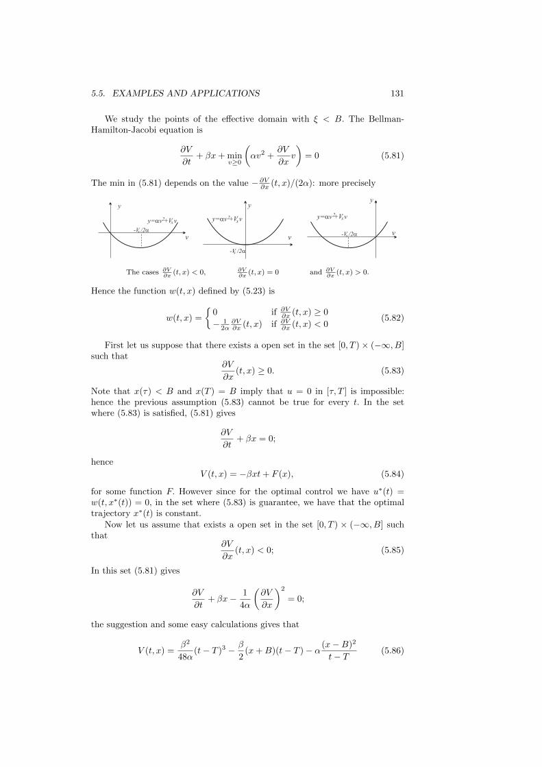
5.5. EXAMPLES AND APPLICATIONS 131
We study the points of the effective domain with ξ < B. The Bellman-Hamilton-Jacobi equation is
∂V
∂t+ βx+ min
v≥0
(αv2 +
∂V
∂xv
)= 0 (5.81)
The min in (5.81) depends on the value −∂V∂x (t, x)/(2α): more precisely
y
v
y= v +V va2
x
-V /2ax
y
v
y= v +V va2
x
-V /2ax
y
v
y= v +V va2
x
-V /2ax
The cases ∂V∂x
(t, x) < 0, ∂V∂x
(t, x) = 0 and ∂V∂x
(t, x) > 0.
Hence the function w(t, x) defined by (5.23) is
w(t, x) =
0 if ∂V
∂x (t, x) ≥ 0
− 12α
∂V∂x (t, x) if ∂V
∂x (t, x) < 0(5.82)
First let us suppose that there exists a open set in the set [0, T )× (−∞, B]such that
∂V
∂x(t, x) ≥ 0. (5.83)
Note that x(τ) < B and x(T ) = B imply that u = 0 in [τ, T ] is impossible:hence the previous assumption (5.83) cannot be true for every t. In the setwhere (5.83) is satisfied, (5.81) gives
∂V
∂t+ βx = 0;
hence
V (t, x) = −βxt+ F (x), (5.84)
for some function F. However since for the optimal control we have u∗(t) =w(t, x∗(t)) = 0, in the set where (5.83) is guarantee, we have that the optimaltrajectory x∗(t) is constant.
Now let us assume that exists a open set in the set [0, T ) × (−∞, B] suchthat
∂V
∂x(t, x) < 0; (5.85)
In this set (5.81) gives
∂V
∂t+ βx− 1
4α
(∂V
∂x
)2
= 0;
the suggestion and some easy calculations gives that
V (t, x) =β2
48α(t− T )3 − β
2(x+B)(t− T )− α (x−B)2
t− T(5.86)

132 CHAPTER 5. OC WITH DYNAMIC PROGRAMMING
satisfies BHJ. Clearly we have to guarantee that (5.85) holds, i.e.
∂V
∂x(t, x) = −β
2(t− T )− 2α
(x−B)
t− T< 0
This implies
x < − β
4α(t− T )2 +B.
Since we are looking for a continuous value function, in the point where it isfinite, equations (5.84) and (5.86) along the line x = − β
4α (t − T )2 + B, i.e.
t = T − 2√
α(B−x)β , gives
−βx
(T − 2
√α(B − x)
β
)+ F (x) =
= −β2
6α
√α3(B − x)3
β3+ β(x+B)
√α(B − x)
β+ α
(x−B)2
2√
α(B−x)β
and hence, with a simple calculation, F (x) = βTx+ 43
√αβ(B − x)3. By (5.84)
we have
V (t, x) = βx(T − t) +4
3
√αβ(B − x)3. (5.87)
Since for this function we require that assumption (5.83) holds, we note that
∂V
∂x= β(T − t)− 2
√αβ(B − x) ≥ 0 ⇔ x ≥ − β
4α(t− T )2 +B.
We obtain that
V (t, x) =
∞ if 0 ≤ t < T and x > B∞ if t = T and x 6= B0 if t = T and x = Bβx(T − t) + 4
3
√αβ(B − x)3 if 0 ≤ t < T, x < B
and x ≥ − β4α (t− T )2 +B
β2
48α (t− T )3 − β2 (x+B)(t− T )− α (x−B)2
t−T if 0 ≤ t < T, x < B
and x < − β4α (t− T )2 +B
Now let us construct the trajectory solving the ODEx = w(t, x) for t ∈ [0, 2]x(0) = A
In order to do that we have that (5.82) becomes
w(t, x) =
0 if 0 ≤ t < T, x < B and x ≥ − β
4α (t− T )2 +Bβ4α (t− T ) + x−B
t−T if 0 ≤ t < T, x < B and x < − β4α (t− T )2 +B
Let us define T = max
(T − 2
√α(B−A)
β , 0
). We have
x = w(t, x) = 0 for t ∈ [0, T )x(0) = A
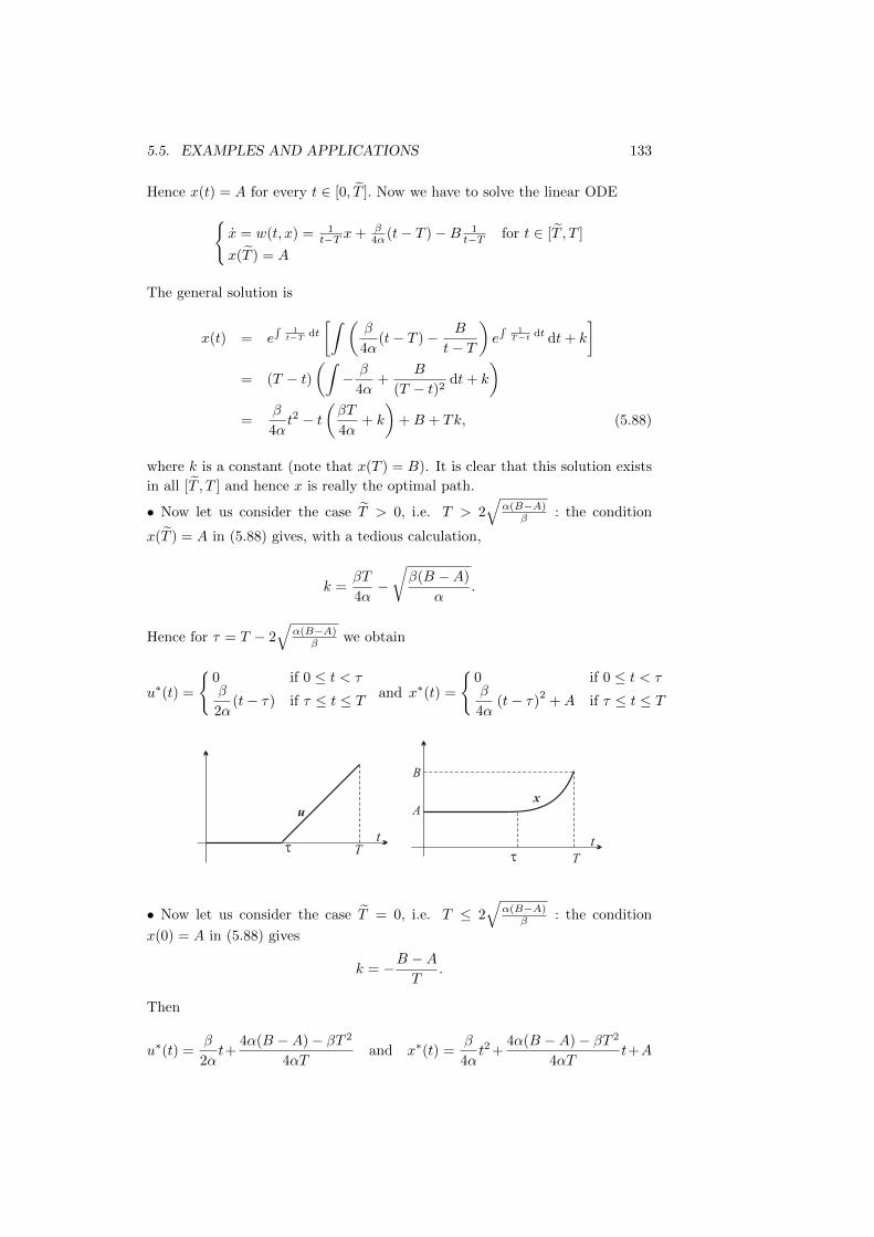
5.5. EXAMPLES AND APPLICATIONS 133
Hence x(t) = A for every t ∈ [0, T ]. Now we have to solve the linear ODEx = w(t, x) = 1
t−T x+ β4α (t− T )−B 1
t−T for t ∈ [T , T ]
x(T ) = A
The general solution is
x(t) = e∫
1t−T dt
[∫ (β
4α(t− T )− B
t− T
)e∫
1T−t dt dt+ k
]= (T − t)
(∫− β
4α+
B
(T − t)2dt+ k
)=
β
4αt2 − t
(βT
4α+ k
)+B + Tk, (5.88)
where k is a constant (note that x(T ) = B). It is clear that this solution exists
in all [T , T ] and hence x is really the optimal path.
• Now let us consider the case T > 0, i.e. T > 2√
α(B−A)β : the condition
x(T ) = A in (5.88) gives, with a tedious calculation,
k =βT
4α−√β(B −A)
α.
Hence for τ = T − 2√
α(B−A)β we obtain
u∗(t) =
0 if 0 ≤ t < τβ
2α(t− τ) if τ ≤ t ≤ T and x∗(t) =
0 if 0 ≤ t < τβ
4α(t− τ)
2+A if τ ≤ t ≤ T
tt
u
T
x
t
t T
B
A
• Now let us consider the case T = 0, i.e. T ≤ 2√
α(B−A)β : the condition
x(0) = A in (5.88) gives
k = −B −AT
.
Then
u∗(t) =β
2αt+
4α(B −A)− βT 2
4αTand x∗(t) =
β
4αt2+
4α(B −A)− βT 2
4αTt+A

134 CHAPTER 5. OC WITH DYNAMIC PROGRAMMING
t
u
T
x
t
T
B
A
Example 5.5.4. Consider the previous model in the particular case T = B = 2, α = 1, andβ = 4. More precisely we consider19
minu
∫ 2
0(u2 + 4x) dt
x = ux(0) = Ax(2) = 2u ≥ 0
where A < 2.
In this case we obtain that
V (t, x) =
∞ if 0 ≤ t < 2 and x > 2∞ if t = 2 and x 6= 20 if t = 2 and x = 2
4x(2− t) +8
3
√(2− x)3 if 0 ≤ t < 2, x < 2
and x ≥ 2− (t− 2)2
1
3(t− 2)3 − 2(x+ 2)(t− 2)−
(x− 2)2
t− 2if 0 ≤ t < 2, x < 2
and x < 2− (t− 2)2
Here τ = 2−√
2−A and the optimal trajectory is
x∗(t) =
A for t ∈ [0, τ ](t− τ)2 +A for t ∈ (τ, 2]
The optimal control is given by
u∗(t) =
0 for t ∈ [0, τ ]2(t− τ) for t ∈ (τ, 2]
In the figure, the domain of the value function V, i.e. the set [0, 2]× R :
19 Suggestion: to solve the PDE Cx + D( ∂V∂x
)2 + E ∂V∂t
= 0 with C, D and E constants,
we suggest to consider the family of functions F (t, x) = a(t− 2)3 + b(x+ 2)(t− 2) + c(x−2)2
t−2,
with a, b, c non zero constants.

5.6. THE MULTIPLIER AS SHADOW PRICE II: THE PROOF 135
• in the yellow subset of dom(V ), i.e. theset
[0, 2]× (2,∞) ∪ (2 × (−∞, 2))
the value function is equal to ∞ sincethere are no controls whose trajectorystarts from to a point of this set and ar-rive in the point (2, 2);
• the red line is an optimal trajectory; onthis red points, i.e. the set [0, 2] × 2,the value function is equal to zero;
• in the points (t, x) of the blue line, i.e.such that x = 2 − (t − 2)2, we have∂V∂x
(t, x) = 0. This blue line divides theset [0, 2]× (−∞, 2), in two regions:
in the upper, we have ∂V∂x
(t, x) >0,
in the lower, we have ∂V∂x
(t, x) < 0;
x
t
2
2
-2
x=2-(t-2)2
2
1
1
• every green line is an optimal trajectory: recalling that the second part of an optimaltrajectory is again an optimal trajectory, starting from generic point a (τ, ξ) on a greenline, we arrive in the point (2, 2) with the optimal path lying on the same green line;
• the blue line divides every trajectory in two parts:
the first part is a segment, i.e. the control is equal to zero,
the second part is a parabola with vertex on the blue line;
• the violet curve is the optimal trajectory with x(0) = 1.
4
5.6 The multiplier as shadow price II: the proof
Let us consider the problemJ(u) =
∫ t1
τ
f(t,x,u) dt
x = g(t,x,u)x(τ) = ξmaxu∈Cτ,ξ
J(u),
(5.89)
with t1 fixed. At this point we know that (with some assumptions)
• by the PMP (2.2) in the Pontryagin theorem 2.1
H(t,x∗(t),u∗(t), λ∗0,λ∗(t)) = max
v∈UH(t,x∗(t),v, λ∗0,λ
∗(t)), (2.2)
for all t ∈ [t0, t1], obtained via a variational approach;
• the BHJ equation (5.8) of theorem 5.1
∂V
∂t(t,x) + max
v∈U
(f(t,x,v) +∇xV (t,x) · g(t,x,v)
)= 0, (5.8)
for all (t,x) ∈ [t0, t1] × Rn, obtained via the approach of the dynamicprogramming.

136 CHAPTER 5. OC WITH DYNAMIC PROGRAMMING
Since in the problem (5.89) the final point of trajectory is free and the final timeis fixed, the optimal control in normal and the Hamiltonian is H = f + λ · g;moreover u∗ is defined as the function that, for every t, associates the value ofv such that realizes the max in (2.2). Taking into account (5.23), the functionthat, for every (t,x), associates the value v that realizes the max in (5.8) is givenby the function w(t,x); such function allow us to define the optimal control, asin (5.25),
u∗(t) = w(t,x∗(t)). (5.90)
A comparison between (2.2) and (5.8) suggests the following result, that wehave announced in remark 2.11: the multiplier λ∗, at every time and along itsoptimal trajectory, provides the sensitivity of the problem (5.89) at the variationof the initial data ξ :
Theorem 5.9. Let x∗t0,α be the optimal trajectory, λ∗t0,α be the optimal mul-tiplier and let V be the value function for the problem 5.89 with initial datax(t0) = α. If V is differentiable, then
∇xV (t,x∗t0,α(t)) = λ∗t0,α(t), (5.91)
for every t ∈ [t0, t1].
The equation (5.91) implies that for a given (τ, ξ) ∈ [t0, t1]×Rn on the optimaltrajectory x∗t0,α, i.e. x∗t0,α(τ) = ξ
x
t1t
a
x= (t)x*t ,a
x*
t0 t
0
t ,a0
we obtain∇xV (τ, ξ) = λ∗t0,α(τ).
Hence, as in remark 2.11, the multiplier λ∗, at time τ, expresses the sensitivity,the “shadow price”, of the optimal value of the problem when we modify theinitial data ξ, along the optimal trajectory.
Proof. (with the additional assumption that V ∈ C2). Let V be the value
function for (5.89) and let x∗ = x∗t0,α be the optimal trajectory. We will provethat if we define the function λ : [t0, t1]→ Rn as
λ(t) = ∇xV (t,x∗(t)), (5.92)
then such function coincides with the multiplier λ∗, i.e. as the unique functionthat solves the ODE in (2.20) in the proof of theorem of Pontryagin 2.1. Thefinal condition (5.5) gives that the value of V (t1,x) does not vary if one modifiesx: hence, by the definition (5.92) of λ, we have
λ(t1) = ∇xV (t1,x∗(t1)) = 0 :

5.6. THE MULTIPLIER AS SHADOW PRICE II: THE PROOF 137
the tranversality condition is proved.Remark 5.3 gives, for every fixed t,
∂V
∂t(t,x∗(t)) = −f(t,x∗(t),u∗(t))−∇xV (t,x∗(t)) · g(t,x∗(t),u∗(t))
= −f(t,x∗(t),u∗(t))−n∑k=1
( ∂V∂xk
(t,x∗(t)) gk(t,x∗(t),u∗(t))).
Considering a derivative with respect to xj we have
∂2V
∂t∂xj(t,x∗(t)) = − ∂f
∂xj(t,x∗(t),u∗(t)) +
−n∑k=1
( ∂2V
∂xk∂xj(t,x∗(t)) gk(t,x∗(t),u∗(t)) +
+∂V
∂xk(t,x∗(t))
∂gk∂xj
(t,x∗(t),u∗(t))). (5.93)
Since V is in C2, the theorem of Schwartz and a derivative with respect to thetime of (5.92) give
λj(t) =∂2V
∂t∂xj(t,x∗(t)) +
n∑i=1
∂2V
∂xj∂xi(t,x∗(t)) x∗i (t)
(by (5.93)) = − ∂f
∂xj(t,x∗(t),u∗(t)) +
−n∑k=1
(∂2V
∂xk∂xj(t,x∗(t)) gk(t,x∗(t),u∗(t)) +
+∂V
∂xk(t,x∗(t),u∗(t))
∂gk∂xj
(t,x∗(t),u∗(t))
)+
+
n∑i=1
∂2V
∂xj∂xi(t,x∗(t)) x∗i (t)
(by dynamics) = − ∂f
∂xj(t,x∗(t),u∗(t)) +
−n∑k=1
∂V
∂xk(t,x∗(t))
∂gk∂xj
(t,x∗(t),u∗(t))
(by (5.91)) = − ∂f
∂xj(t,x∗(t),u∗(t)) +
−n∑k=1
λk(t)∂gk∂xj
(t,x∗(t),u∗(t)). (5.94)
Hence the function λ solves the ODEλ(t) = −λ(t) · ∇xg(t,x∗(t),u∗(t))−∇xf(t,x∗(t),u∗(t))λ(t1) = 0
that is exactly the ODE (2.20) in the theorem of Pontryagin. The uniquenessof the solution of such ODE implies λ = λ∗. The relation (5.94) is the adjointequation.

138 CHAPTER 5. OC WITH DYNAMIC PROGRAMMING
5.7 Infinite horizon problems
Let us consider the problem, for r > 0,J(u) =
∫ ∞0
e−rtf(x,u) dt
x = g(x,u)x(0) = αmax
u∈C0,αJ(u)
(5.95)
If we consider the value function V : [0,∞) × Rn → [−∞,∞] of this problem,it satisfies the BHJ equation
∂V
∂t(t,x) + max
v∈U
(e−rtf(x,v) +∇xV (t,x) · g(x,v)
)= 0, ∀(t,x) ∈ [0,∞)× Rn
(5.96)where U ⊂ Rk is, as usual, the control set. We remark that
V (τ, ξ) = maxu∈Cτ,ξ
∫ ∞τ
e−rtf(x,u) dt
= e−rτ maxu∈Cτ,ξ
∫ ∞τ
e−r(t−τ)f(x,u) dt
(with s = t− τ) = e−rτ maxu∈C0,ξ
∫ ∞0
e−rsf(x, u) ds.
Two comments on the last equality. Since g does not depend explicitly by t,the function u : [0,∞) → U is such that u ∈ C0,ξ if and only if the functionu : [τ,∞) → U , with u(t) = u(τ + t), is such that u ∈ Cτ,ξ. Essentially, theclasses of functions Cτ,ξ and C0,ξ contain the same object. Moreover, for therespectively trajectory x and x we have x(t) = x(τ + t).
The last integral depends on the initial value x, but it does not depend on theinitial time τ. Hence we define the current value function20 V c : Rn → [−∞,∞]as
V c(ξ) = maxu∈C0,ξ
∫ ∞0
e−rtf(x,u) dt;
hence
V c(x) = ertV (t,x). (5.97)
From (5.96) we have
−rV c(x) + maxv∈U
(f(x,v) +∇V c(x) · g(x,v)) = 0, ∀x ∈ Rn. (5.98)
Such new BHJ is called Bellman–Hamilton–Jacobi equation for the current valuefunction. The BHJ equation for the current value function is very useful sinceit is not a PDE, but an ODE.
The final condition on the value function for the problem is
limt→∞
V (t,x) = 0;
20We remark that V c depends only on x and hence ∇xV c(x) = ∇V c(x).

5.7. INFINITE HORIZON PROBLEMS 139
clearly, using (5.97), we obtain that the final condition is automatically guaran-teed for the function V c.
If we define wc : Rn → Rk as the value v such that realizes the max in theprevious equation, i.e.
wc(x) ∈ arg maxv∈U
(f(x,v) +∇V c(x) · g(x,v)) , (5.99)
it is easy to see that
w(t,x) = wc(x), ∀t ∈ [t0, t1], x ∈ Rn
where w is defined in (5.23). Hence, in order to guarantee some sufficient con-dition of optimality and to find the optimal control, we have to guarantee theexistence of x∗ solution of the ODE (5.24), i.e.
x(t) = g(t,x, wc(x)
)in [t0, t1]
x(t0) = α.(5.100)
Then x∗ is the optimal trajectory and u∗, defined by (5.25), i.e.
u∗(t) = w(t,x∗(t)), (5.101)
is the optimal control.
Example 5.7.1. Let us consider21min
∫ ∞0
e−rt(ax2 + bu2) dt
x = ux(0) = x0 > 0a, b fixed and positive
The current value function V c = V c(x) must satisfy (5.98), i.e.
−rV c + minv∈R
(ax2 + bv2 + (V c)′v
)= 0
=⇒ −rV c + ax2 + minv∈R
(bv2 + (V c)′v
)= 0. (5.102)
The function v 7→ bv2 + (V c)′v is, for every fixed x, a parabola; since b is positive
wc(x) = −(V c)′/(2b). (5.103)
Hence (5.102) becomes4brV c − 4abx2 + [(V c)′]2 = 0. (5.104)
We looking for the solution in the homogenous polynomials on x of degree two, i.e. as thefunctions V c(x) = Ax2, with A ∈ R : replacing this expression in the (5.104) we have
4brAx2 − 4abx2 + 4A2x2 = 0 =⇒ A2 + brA− ab = 0 =⇒ A± =−br ±
√b2r2 + 4ab
2.
From the problem it is clear that the current value function V c and the value function V =V ce−rt are non negative: hence we consider only A+, i.e.
V c(x) =−br +
√b2r2 + 4ab
2x2. (5.105)
and, from (5.103) we have
wc(x) =br −
√b2r2 + 4ab
2bx.
21In the example 3.7.1 we solve the same example with the variational approach.

140 CHAPTER 5. OC WITH DYNAMIC PROGRAMMING
In order to find the optimal trajectory, the ODE (5.100) isx(t) =
br−√b2r2+4ab2b
x(t)x(0) = x0.
and its unique solution is
x∗(t) = x0e
(br−√b2r2+4ab
)t/(2b)
. (5.106)
The (5.101) gives us the optimal control
u∗(t) = wc(x∗(t)) =br −
√b2r2 + 4ab
2bx0e
(br−√b2r2+4ab
)t/(2b)
.
4
Consider the problem (5.95). Using theorem 5.9 it is very easy to see that theinterpretation of the current multiplier is similar: recalling (3.100) and (5.97),i.e.
λ∗c = ertλ∗ and V (t,x) = e−rtV c(x),
then (5.91) gives, dropping the apex t0,α,
Remark 5.7.
∇V c(x∗(t)) = λ∗c(t),
for every t ∈ [t0, t1]. The current multiplier is the sensitivity of the current valuefunction if we chance the initial state, along the optimal trajectory.
Example 5.7.2. Let us consider 22
min
∫ ∞0
e−rt(ax2 + bu2) dt
x = ux(0) = x0 > 0a, b fixed and positive
We want to verify the relation in Remark 5.7.
The solution of example 3.7.1 and example 5.7.1 give (see (3.109), (3.110), (5.105) and(5.106))
x∗(t) = x0e
(br−√b2r2+4ab
)t/(2b)
,
λ∗c(t) = x0(√
b2r2 + 4ab− br)e
(br−√b2r2+4ab
)t/(2b)
,
V c(x) =−br +
√b2r2 + 4ab
2x2.
Clearly these equations give
∇V c(x∗(t)) =dV c
dx(x∗(t)) = 2x∗(t)
−br +√b2r2 + 4ab
2= λ∗c(t).
4
22In the example 3.7.1 and in example 5.7.1 we solve the example with the variational andthe Dynamic Programming approach respectively.

5.7. INFINITE HORIZON PROBLEMS 141
5.7.1 Particular infinite horizion problems
We note that many of the arguments in the first part of this section hold whenwe consider the case r = 0. In particular
Remark 5.8. Let us consider the problemmax
u∈C0,α
∫ ∞0
f(x,u) dt
x = g(x,u)x(0) = α
Then we value function does not depend directly by t, i.e. V (t,x) = V (x).Moreover the BHJ equation is
maxv∈U
(f(x,v) +∇V (x) · g(x,v)) = 0.
In the spirit of Proposition 5.4, taking into account the previous remark, wehave that
Remark 5.9. Let us consider the autonomous Affine Quadratic infinite horizonproblem
maxu∈C0,α
1
2
∫ ∞0
(x′Qx + 2x′S + u′Ru) dt
x = Ax +Bu + Cx(0) = α
where the matrices Q, S, R,A,B and C are constants. Moreover we assumeQ ≤ 0 and R < 0. Then the value function is of the type
V (t,x) = V (x) =1
2x′Zx +Wx + Y
where Z, W and Y are constant matrices.
5.7.2 A model of consumption with HARA–utility
We solve the model presented in the example 1.1.5, formulated with (1.6) witha utility function
U(c) =1
γcγ ,
where γ is fixed in (0, 1): this is a commonly used utility function, of so calledHARA type23. Our problem24 is
max
∫ ∞0
1
γcγe−δt dt
x = rx− cx(0) = x0 > 0x ≥ 0c ≥ 0
(5.107)
23In economics Hyperbolic Absolute Risk Aversion (HARA) refers to a type of risk aversionthat is particularly convenient to model mathematically and to obtain empirical prediction.
24Note that here we remove from the model the assumption limt→∞ x(t) = 0.

142 CHAPTER 5. OC WITH DYNAMIC PROGRAMMING
We will show that two situations occur depending on the fixed constants r, γand δ: the case 0 < rγ < δ and the case 0 < δ ≤ rγ.
A generalization of this model is the fundamental Merton model that we willintroduce in subsection 5.7.3.
The case δ > rγ : the current value function V c = V c(x) must satisfy (5.98),i.e.
−δV c + maxv≥0
(1
γvγ + (V c)′(rx− v)
)= 0
=⇒ −δV c + (V c)′rx+ maxv≥0
(1
γvγ − (V c)′v
)= 0. (5.108)
Now, since for definition
V c(ξ) = maxc
∫ ∞0
1
γcγe−δt dt with x(0) = ξ,
if the initial wealth ξ increases, then it is reasonable that the utility increases,i.e. we can suppose that (V c)′ > 0. Hence, recalling the definition (5.99),
wc(x) = [(V c)′]1
γ−1 = arg maxv≥0
(1
γvγ − (V c)′v
)(5.109)
and the BHJ equation for V c (5.108) becomes
−δV c + (V c)′rx+1− γγ
[(V c)′]γγ−1 = 0, ∀x ≥ 0.
In order to solve the previous ODE, let us consider a function of the type
V c(x) = Axγ , x ≥ 0,
where A is a positive constant (coherent with the assumption (V c)′ > 0) : weobtain
−δAxγ +Aγrxγ +1− γγ
[γAxγ−1]γγ−1 = 0, ∀x ≥ 0.
An easy calculation, together with the assumption δ > rγ, gives
A =1
γ
(1− γδ − γr
)1−γ
> 0.
Now (5.109) implies that the function w in Theorem 5.3 is given by (recallingthe wc(x) = w(t, x))
wc(x) = [(V c)′]1
γ−1 =δ − γr1− γ
x.
In our contest, the ODE (5.100) becomes x =r − δ1− γ
x
x(0) = x0

5.7. INFINITE HORIZON PROBLEMS 143
Its solution is x∗(t) = x0er−δ1−γ t : let us note that the condition x∗(t) ≥ 0 is
satisfied. Hence Theorem 5.3 guarantees that x∗,
c∗(t) = wc(x∗(t)) = x0δ − γr1− γ
er−δ1−γ t and V (t, x) =
1
γ
(1− γδ − γr
)1−γ
e−βtxγ ,
for every x ≥ 0, t ≥ 0, are the optimal trajectory, the optimal consumptionplain and the value function for the investor’s problem respectively. Finally wenote that for such optimal solution we have
c∗(t)
x∗(t)=δ − γr1− γ
, ∀t ≥ 0,
i.e. in the optimal plain the ratio between consumption and wealth is constant.
The case δ ≤ rγ : Let us show that in this second case we have that the valuefunction is equal to∞ and hence an optimal path of consumption does not exist.
Let us consider a fixed constant A > 0 and the path of consumption cA(t) =Aert, for t ≥ 0 : let us show that this control is not admissible. The dynamicsand the initial condition on the wealth give
x = rx−Aertx(0) = x0
and its solution is xA(t) = ert(x0 − At) : note that the condition x(t) ≥ 0 issatisfied for t ≤ x0/A : hence cA is not and admissible control. Now we considera modification of the previous path of consumption (that we denote again withcA):
cA(t) =
Aert for 0 ≤ t ≤ x0
A ,0 for t > x0
A
(5.110)
The dynamics and the initial condition give now
xA(t) =
ert(x0 −At) for 0 ≤ t ≤ x0
A ,0 for t > x0
A
Hence, for every initial wealth x0 > 0 and for every A > 0, the control cA givenby (5.110) is admissible and
V c(x0) = V (0, x0) = supc
∫ ∞0
1
γcγe−δt dt
≥ limA→0+
∫ ∞0
1
γcγAe−δt dt
= limA→0+
∫ x0/A
0
Aγ
γe(γr−δ)t dt
≥ limA→0+
∫ x0/A
0
Aγ
γdt =∞,
where, using the assumption, we use the fact that e(γr−δ)t ≥ 1 for every t ≥ 0.Hence V c(x0) = ∞, for every x0 > 0, implies V (t, x) = ∞, for every (t, x) ∈[0,∞)× (0,∞).

144 CHAPTER 5. OC WITH DYNAMIC PROGRAMMING
5.7.3 Stochastic consumption: the idea of Merton’s model
A generalization of the problem (5.107) is the fundamental Merton’s model (see[21]), where an investor divides the wealth between consumption, a riskless assetwith rate r and a risk asset with uncertain rate return: it is a stochastic modelin the context of stochastic optimal control. The aim of this subsection is onlyto give and idea of the problem (see [18], [13], [12] for details).
In this model, the stock portfolio consists of two assets:
• the price p1 = p1(t) for the “risk free” asset changes according to p1 = rp1,i.e.
dp1 = rp1 dt, (5.111)
where r is a positive constant;
• the price p2 = p2(t) for the “risk ” asset changes according to
dp2 = sp2 dt+ σp2 dBt, (5.112)
where Bt is a Brownian motion, s and σ are positive constants: s formal-izes the expected profit for the risk investment and σ is its variance.
It is reasonable, for the investor’s point of view, to require
0 < r < s.
According to (5.111) and (5.112), the total wealth x = x(t), evolves as
dx = [r(1− w)x+ swx− c] dt+ wxσ dBt, (5.113)
where c = c(t) is, as in (5.107), the consumption and w = w(t) is the fraction(i.e. 0 ≤ w ≤ 1) of the remaining wealth invested in the risk asset. We note thatif we put w(t) = 0 in (5.113), then we obtain the dynamic in problem (5.107).
Again, we have a HARA utility function for the consumption to maximize,in the sense of the expected value since w, x and c are all random variables:hence we obtain
max(c,w)
E(∫ ∞
0
cγ
γe−δt dt
)dx = [r(1− w)x+ swx− c] dt+ wxσ dBtx(0) = x0 > 0c ≥ 00 ≤ w ≤ 1
(5.114)
with γ constant in (0, 1).
5.7.4 A model of consumption with log–utility II
We solve25 the model presented in the example 1.1.5, formulated with (1.6), inthe case δ > r and with a logarithmic utility function U(c) = log c. The currentvalue function V c = V c(x) must satisfy (5.98), i.e.
−δV c + maxv≥0
(ln v + (V c)′(rx− v)) = 0
=⇒ −δV c + (V c)′rx+ maxv≥0
(ln v − (V c)′v) = 0. (5.115)
25In subsection 3.7.1 we solve the same problem with the variational approach.

5.7. INFINITE HORIZON PROBLEMS 145
Now, since for definition
V c(ξ) =
∫ ∞0
e−δt ln cdt with x(0) = ξ,
if the initial capital ξ increases, then it is reasonable that the utility increases,i.e. we can suppose that (V c)′ > 0. Hence
wc(x) =1
(V c)′= arg max
v≥0(ln v − (V c)′v) (5.116)
and the BHJ equation for V c (5.115) becomes
−δV c + (V c)′rx− ln[(V c)′]− 1 = 0, ∀x ≥ 0. (5.117)
In order to solve the previous ODE, let us consider a derivative with respect tox of it; we obtain
−δ(V c)′ + (V c)′′rx+ (V c)′r − (V c)′′
(V c)′= 0, ∀x ≥ 0.
Now suppose that (V c)′ is a homogeneous polynomial of degree k in the variablex, i.e. (V c)′ = Axk with A constant. Then we obtain
−δAxk + krAxk + rAxk − k 1
x= 0, ∀x ≥ 0;
for k = −1, the previous equation is homogeneous and we obtain A = 1δ that
implies V c(x) = ln(δx)δ + B, for some constant B. If we replace this expression
for V c in (5.117) we obtain
−δ(
ln(δx)
δ+B
)+r
δ+ ln(δx)− 1 = 0, ∀x ≥ 0,
that implies B = r−δδ2 , i.e.
V c(x) =1
δ
(ln(δx) +
r − δδ
), ∀x ≥ 0.
We don’t know if it’s the general solution for the BHJ equation (5.115), butsure it is a solution. Now (5.116) implies that
wc(x) = δx.
In our contest, the ODE (5.100) becomesx = (r − δ)xx(0) = x0
Its solution is x(t) = x0e(r−δ)t : let us note that the condition x(t) ≥ 0 and
limt→∞ x(t) = 0 are satisfied. Hence Theorem 5.3 guarantees that
c(t) = δx0e(r−δ)t and V (t, x) =
e−δt
δ
(ln(δx) +
r − δδ
), ∀x ≥ 0, t ≥ 0,
are the optimal consumption plain and the value function for the investor’sproblem.

146 CHAPTER 5. OC WITH DYNAMIC PROGRAMMING
5.8 Problems with discounting and salvage value
Let us consider the problem (see [28]), for a fixed final time T > 0,J(u) =
∫ T
0
e−rtf(t,x,u) dt+ e−rTψ(x(T ))
x = g(t,x,u)x(0) = αmaxu∈U
J(u)
(5.118)
where r > 0 is a given discount rate and ψ is the pay-off function (or salvage
value). We define the function f by
f(t,x,u) = e−rtf(t,x,u) + e−rT∇ψ(x) · g(t,x,u). (5.119)
It is easy to see that for the new functional J we have
J(u) =
∫ T
0
f(t,x,u) dt
=
∫ T
0
e−rtf(t,x,u) dt+ e−rT∫ T
0
∇ψ(x(t)) · g(t,x,u) dt
=
∫ T
0
e−rtf(t,x,u) dt+ e−rT∫ T
0
dψ(x(t))
dtdt
= J(u)− e−rTψ(α);
hence the new objective function J differs from the original objective functionalJ only by a constant. So the optimization problem remains unchanged whensubstituting f with f (i.e. the optimal controls of the two problems are the
same). The BHJ-equation of the problem “”(with value function V ) is
−∂V∂t
(t,x) = maxv∈U
(f(t,x,v) +∇xV (t,x) · g(t,x,v)
)= e−rt max
v∈U
(f(t,x,v) + ert(∇xV (t,x) + e−rT∇ψ(x)) · g(t,x,v)
),
and the final condition is V (T,x) = 0. Let us define
V c(t,x) = ert(V (t,x) + e−rTψ(x)
); (5.120)
we obtain
−rV c(t,x) +∂V c
∂t(t,x) + max
v∈U(f(t,x,v) +∇xV
c(t,x) · g(t,x,v)) = 0, (5.121)
V c(T,x) = ψ(x). (5.122)
It is clear that
arg maxv∈U
(f(t,x,v) +∇xV (t,x) · g(t,x,v)
)=
= arg maxv∈U
(f(t,x,v) +∇xV
c(t,x) · g(t,x,v)).

5.8. PROBLEMS WITH DISCOUNTING AND SALVAGE VALUE 147
It is easy to see that, given an optimal control u∗ for the initial problem (5.118),we have by (5.119) and (5.120)
V c(t,x∗(t)) = ert(V (t,x∗(t)) + e−rTψ(x∗(t))
)= ert
(∫ T
t
f(s,x∗,u∗) ds+ e−rTψ(x∗(t))
)
=
∫ T
t
e−r(s−t)f(s,x∗,u∗) ds+
+e−r(T−t)
(∫ T
t
∇ψ(x∗) · g(s,x∗,u∗) ds+ ψ(x∗(t))
)
=
∫ T
t
e−r(s−t)f(s,x∗,u∗) ds+ e−r(T−t)ψ(x∗(T )).
Hence V c(t,x∗(t)) is the optimal discounted (at time t) value or, in analogywith (5.97), the current value function for (5.118). The equation (5.121) iscalled Bellman–Hamilton–Jacobi equation with discounting and salvage value.
5.8.1 A problem of selecting investment
Consider the firm’s problem of selecting investment in the fixed period [0, T ].The profit rate, exclusive of capital costs, that can be earned with a stockof productive capital k is proportional to k2. The capital stock decays at aconstant proportionate rate26 α, so k = ı−αk, where ı is gross investment, thatis, gross additions of capital. The cost of gross additions of capital at rate ıis proportional to ı2. At the end of the investment period, the firm receives anadditional profit on an asset (for example, a coupon) of a value proportional tothe square of the final capital. We seek to maximize the present value of thenet profit stream over the period [0, T ] :
max
∫ T
0
e−rt(ρk2 − σı2) dt+ πe−rT k(T )2
k = ı− αkk(0) = k0 > 0ı ∈ I
where α, σ, π and r are fixed positive constants such that σα2 > ρ and I ⊂R is convex, compact and large enough (so as to allow for an unconstrainedminimization).
Conditions (5.121) and (5.122) give, for the optimal discounted value func-tion V c = V c(t, k),
−rV c +∂V c
∂t+ max
v∈I
(ρk2 − σv2 + (v − αk)
∂V c
∂k
)= 0,
V c(T, k) = πk2.
26If a stock k decays at a constant proportionate rate β > 0 and if it is not replenished,then k(t)/k(t) = −β. Since the solution of this ODE is k(t) = k(0)e−βt, we sometimes saythat the stock k decays exponentially at rate β.

148 CHAPTER 5. OC WITH DYNAMIC PROGRAMMING
Let us assume that V c(t, k) = q(t)k2; we obtain
−(2α+ r)qk2 + q′k2 + ρk2 + maxv∈I
(−σv2 + 2kqv
)= 0,
q(T ) = π.
The assumption on I implies that
ı = arg maxv∈I
(−σv2 + 2kqv
)=kq
σ(5.123)
and the BHJ now is, after a division by k2,
q′ = −ρ+ (2α+ r)q − q2
σ(5.124)
In order to solve this Riccati equation in q (see the footnote in example 5.5.2)with the condition q(T ) = π, let us introduce the new variable z = z(t) with
q = σz′
z, z(T ) = σ, z′(T ) = π.
This implies q′ = σ z′′z−(z′)2z2 and, by (5.124),
z′′ − 2(α+
r
2
)z′ +
ρ
σz = 0.
Let us set, by assumption, θ =√
(α+ r/2)2 − ρ/σ > 0 : hence
z(t) = e(α+r2+θ)(t−T )
(c1 + c2e
−2θ(t−T )).
This implies
z′(t) = e(α+r2+θ)(t−T )
(c1
(α+
r
2+ θ)
+ c2
(α+
r
2− θ)e−2θ(t−T )
)and conditions z(T ) = σ, z′(T ) = π allow us to determinate the two constantsc1 and c2 :
c1 =π −
(α+ r
2 − θ)σ
2θ, c2 =
(α+ r
2 + θ)σ − π
2θ.
Condition (5.123) gives, for every t ∈ [0, T ], that the candidate to be the optimal
investment (i.e. control) is ı = kq/σ and using q = σz′/z we obtain ı = kz′
z. If
we substitute this expression of ı in the dynamics we obtain
k′ = kz′
z− αk ⇒
∫1
kdk =
∫ (z′
z− α
)dt+ c
⇒ k = zfe−αt
with c and f constants. The initial condition on the capital gives
k(t) =k0z(0)
z(t)e−αt
and hence the optimal path of investment is given by
ı∗(t) =k0z(0)
e−αtz′(t) =k0z(0)
e(r2+θ)t
(c1
(α+
r
2+ θ)
+ c2
(α+
r
2− θ)e−2θt
)

Index
H, 11H0, 20Hc, 79KC, 5V , 105V c, 138, 140, 147λc, 79wc, 140Ct0,α, 8
abnormal control, 12example, 28
absolutely continuous function, 6adjoint equation, 11
AE, 11Affine Quadratic problems, 113autonomous optimal control problem,
9properties, 15, 46, 47
BellmanPrinciple of optimality, 107
Bellman-Hamilton-Jacobi equation, 108,122
for the current value function, 138with discounting and salvage value,
147BHJ equation, 108, 122
calculus of variation, 22Bolza problem, 55infinite horizon problem, 75transversality condition, 23, 75
constrained optimal control problemconstraint qualification, 86
control, 8abnormal, 12, 28admissible, 8bang-bang, 36extremal, 12normal, 12
optimal, 9set, 5singular, 36
controllability, 8matrix, 63
costate variable, 11CoV, 22
dynamics, 6linear, 8
Euler equation, 23EU, 23for the Lagrangian in isoperimet-
ric problems of CoV, 98exit time, 46extremal
for the Lagrangian in isoperimet-ric problems of CoV, 98
in calculus of variation, 23in optimal control, 11
Gronwall’s inequality, 59
Hamiltonian, 11constrained problems, 86current, 79for Dynamic Programming, 111maximized, 20, 31
Lagrangiangeneralized in isoperimetric prob-
lems of CoV, 96in constraints problem of OC, 87in isoperimetric problems of CoV,
97Linear Quadratic problems
homogeneous, 115LQ problems, 113
Maximum Principle of Pontryagin, 11PMP0, 13
149
150 INDEX
PMP, 11multiplier, 11
as “shadow price”, 42, 136associated, 12current, 79, 140
normal control, 12sufficient condition, 13, 45
OC, 9optimal control problem
autonomous, 9, 88of Bolza, 43of Lagrange, 43of Mayer, 43
optimal in CoV, 22optimal time, 64
pay off, 43pay off function, 9
rank condition, 86reachable set, 8, 63, 122Riccati differential equation, 124running cost, 9
solution of ODE, 7switching point, 36
target set, 5, 122theorem
Arrow, 20Euler, 22Mangasarian, 18Pontryagin, 11, 16, 48
time optimal problem, 64linear, 63
trajectory, 5, 8optimal, 9
transversality condition, 11Halkin counterexample, 73in calculus of variation, 23, 75in time optimal problem, 64infinite horizon problem, 73TC, 11with fixed final time, 45with free final time, 46
utility functionHARA, 141, 144log, 82, 144
value function, 105V , 105V c, 140current, 138, 140, 147final condition, 106, 122necessary condition, 108, 122regularity, 116sufficient condition, 111, 122viscosity solution, 120

Bibliography
[1] A. Agracev and Y. Sachkov. Control theory from the geometric viewpoint.Springer, 2003.
[2] K. J. Arrow. Applications of control theory of economic growth. Mathe-matics of Decision Sciences, part 2, AMS, page 92, 1968.
[3] M. Bardi and I. Capuzzo Dolcetta. Optimal Control and Viscosity Solutionsof Hamilton–Jacobi–Bellman Equations. Birkhauser, Boston, 1997.
[4] T. Basar and G.J. Olsder. Dynamic Noncooperative Game Theory. SIAMClassic in Applied Mathematics, 1998.
[5] B. Beavis and I. Dobbs. Optimization and stability for economic analysis.Cambridge university press.
[6] R. Bellman. Dynamic programming. Princeton University Press, 1957.
[7] A. Calogero. Appunti di calcolo delle variazioni e controllo ottimo. avaibleon the web site www.matapp.unimib.it/∼calogero/.
[8] M.C. Caputo. Foundation of dynamic economic analysis: optimal controltheory and applications. Cambridge University Press, 2005.
[9] A.C. Chiang. Dynamic optimization. McGraw-Hill international editions.
[10] L.C. Evans. An Introduction to Mathematical Optimal Control Theory.available in the web site of Prof. L.C. Evans (Berkley University).
[11] L.C. Evans. Partial Differental Equation. American Mathematical Society,2010.
[12] L.C. Evans. An introduction to stochastic differential equations. avaible onthe web site http://math.berkeley.edu/evans, version 1.2.
[13] W.H. Fleming and P.W. Rishel. Deterministic and stochastic optimal con-trol. Springer-Verlag, 1975.
[14] R. Gamkrelidze. Principles of Optimal Control Theory. Plenum Press,1978.
[15] A. Haurie, J.B. Krawczyk, and G. Zaccour. Games and dynamic games.World Scientific, 2012.
151

152 BIBLIOGRAPHY
[16] H. Hotteling. The economics of exhaustible resources. Journal of PoliticalEconomic, pages 137–175, April 1931.
[17] M. I. Kamien and N.L. Schwartz. Dynamic optimization. Elsevier, 2006.
[18] B. Øksendal. Stochastic differential equations. Springer, 2007.
[19] D. Leonard and N. Van Long. Static optimization in economics. Cambridgeuniversity press.
[20] O. L. Mangasarian. Sufficient conditions for the optimal control nonlinearsystems. SIAM Journal on control, 4:139–152, 1966.
[21] R. C. Merton. Lifetime portofolio selection under uncertainty: thecontinuous–time case. Rev. Econ. Statist., pages 247–257, August 1969.
[22] L.S. Pontryagin, V.G. Boltyanskii, R.V. Gamkrelidze, and E.F.Mishchenko. The mathematical theory of optimal process. Intersciencepublishers, John Wiley & Sons.
[23] F. P. Ramsey. A mathematical theory of saving. Economic Journal, pages543–559, December 1928.
[24] R.T. Rockafellar. Convex Analysis. Princeton University Press, 1969.
[25] S. Salsa and A. Squellati. Modelli dinamici e controllo ottimo. Egea.
[26] A. Seierstad and K. Sydsæter. Optimal control theory with economics ap-plications. Elsevier Science, 1987.
[27] A. Takayama. Mathematical economics. second edition, Cambridge univer-sity press.
[28] T. A. Weber. Optimal control theory with applications in economics. TheMIT Press, 2011.