notes on producer theory - university of...

Notes on Producer Theory

Alejandro Saporiti

Alejandro Saporiti (Copyright) Producer Theory 1 / 27

Producer theory

Reference:Jehle and Reny,Advanced Microeconomic Theory, 3rd ed.,Pearson 2011: Ch. 3.

The second important actor in economics is the firm (producer).

We begin with aspects of production and costs that are commonto all firms.Then we consider the behavior of competitive firms, a very special butimportant class of firms.

A firm (producer) carries out the production process transforming inputs intooutputs. To do that, the firm employs a certaintechnology.

If the firm produces a single product from many inputs, its technology can berepresented by a production function.


Producer theory

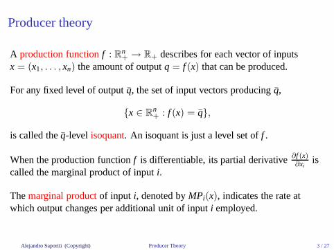
A production functionf : Rn+ → R+ describes for each vector of inputs

x = (x1, . . . , xn) the amount of outputq = f (x) that can be produced.

For any fixed level of outputq, the set of input vectors producingq,

{x ∈ Rn+ : f (x) = q},

is called theq-level isoquant. An isoquant is just a level set off .

When the production functionf is differentiable, its partial derivative∂f (x)∂xi

iscalled the marginal product of inputi.

Themarginal productof input i, denoted byMPi(x), indicates the rate atwhich output changes per additional unit of inputi employed.


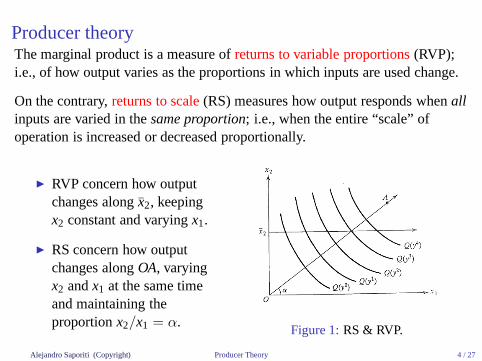
Producer theoryThe marginal product is a measure ofreturns to variable proportions(RVP);i.e., of how output varies as the proportions in which inputsare used change.

On the contrary,returns to scale(RS) measures how output responds whenallinputs are varied in thesame proportion; i.e., when the entire “scale” ofoperation is increased or decreased proportionally.

◮ RVP concern how outputchanges alongx2, keepingx2 constant and varyingx1.

◮ RS concern how outputchanges alongOA, varyingx2 andx1 at the same timeand maintaining theproportionx2/x1 = α.

Figure 1:RS & RVP.


Producer theoryA production functionf : R

n+ → R+ has the property of:

1. Constant returns to scaleif for all t > 0 andx ∈ Rn+, f (t x) = t f (x);

2. Increasing returns to scaleif for all t > 1 andx ∈ Rn+, f (t x) > t f (x);

3. Decreasing returns to scaleif for all t > 1 andx ∈ Rn+, f (t x) < t f (x).

If the production function is homogenous, returns to scale can be associatedwith the degree of homogeneity.

N.B. Recall that a production functionf : Rn+ → R+ is homogeneous of

degreek if for all λ > 0 andx ∈ Rn+, f (λ x) = λk f (x); (e.g. f (x1, x2) = xα

1 xβ2

is homogeneous of degreek = α + β).

◮ If the production function is homogeneous of degreek > 1 (k < 1), itmust exhibitincreasing(decreasing) RS; the converse need not hold.

◮ If the production function is homogeneous of degreek = 1, it hasconstantRS, and viceversa.


Producer theory

As we did in consumer theory with the MRS, it is possible to investigate herethe rate at which one input can be substituted by another without changing theamount of output produced.

This rate is given by themarginal rate of technical substitution(MRTS).

Whenn = 2, MRTS12(x) is obtained by totally differentiatingf (x1, x2) = q:

dq =∂f (x1, x2)

∂x1dx1 +

∂f (x1, x2)

∂x2dx2 = 0.

⇒dx2

dx1

∣

∣

∣

dq=0= −

∂f (x1,x2)∂x1

∂f (x1,x2)∂x2

= −MP1(x1, x2)

MP2(x1, x2)= MRTS12(x1, x2).

TheMRTS12(x) is the slope atx of the isoquant passing throughq.


Producer theory

More generally, whenn > 2 for any two inputsi 6= j,

MRTSij(x) = −MPi(x)MPj(x)

.

In the two input case, the production functionf (x1, x2) exhibits adiminishingMRTSif for any q, the absolute value of MRTS,|MRTS12|, diminishes asx1

increases andx2 is restricted by the isoquantf (x1, x2) = q.

◮ A diminishing MRTS is consistent with increasing marginalproductivities;

◮ A diminishing MRTS implies that the slope of the isoquantin absolutevalue is decreasing (i.e. that the isoquants are convex).

The MRTS is onelocal measure of substitutability between inputs inproducing a given level of output.


Producer theory

Theelasticity of substitutionof input j for input i is defined as the % changein the proportionsxj/xi associated with a one % change in theMRTSij,holding all other inputs and the level of output constant.

For a production functionf (x), the elasticity of substitution of inputj for inputi at x0 ∈ R++ is defined as

σij(x0) =

(

d ln MRTSij(x(r))d ln r

∣

∣

∣

r=x0j /x0

i

)−1

, (1)

wherex(r) is the unique vector of inputsx = (x1, . . . , xn) such that (i)xj/xi = r, (ii) xk = x0

k for all k 6= i, j, and (iii) f (x) = f (x0).

The elasticity of substitutionσij(x0) is a measure of the curvature of thei − jisoquant throughx0 at x0.


Producer theoryWhen the production functionf is quasi-concave,σij ≥ 0; (convex isoquantsimply that↑ (x2/x1) ⇒ ↑ |MRTS12|).

The closerσij is to zero, the more difficult is the substitution between inputs jandi; the larger it is, the easier is the substitution between them.

Figure 2:Elasticity of substitution.

In Fig 2, panel (a) representsperfect substitutability; panel (c)nosubstitutability(fixed proportions); and panel (b) an intermediate case.


Producer theory

Consider a firm (producer) that looks for theoptimal demand of each inputxi,i = 1, . . . , n, to minimize the cost of producingq units of output, given theprevailing technologyf (·) and the input pricesp = (p1, . . . , pn) ≫ 0.

Thecost minimization problem(CMP) of the firm takes the form

minx1,...,xn

p1x1 + . . . + pnxn subject to f (x1, . . . , xn) ≥ q. (2)

The objective function is linear in the decision variablesx1, . . . , xn.

Hence, if the production functionf (·) exhibits “some kind of concavity” andthere is an interior solution, (2) can be solved using the Lagrange method.

The solution, denoted byxci (p, q), determines theconditional demand for

input i = 1, . . . , n, (conditional on the output levelq).


Producer theory

Unfortunately, not all production functions are concave.

For instance, theCobb-Douglas production functionf (x1, x2) = k xα1 xβ

2 , withk, α, β > 0, has a Hessian matrix

Hf (x1, x2) =

(

k α (α − 1) xα−21 xβ

2 k αβ xα−11 xβ−1

2

k α β xα−11 xβ−1

2 k β (β − 1) xα1 xβ−2

2

)

.

The elements of the main diagonal are non-positive ifα ≤ 1 andβ ≤ 1.

The determinant|Hf (x1, x2)| = k2 x2(α−1)1 x2(β−1)

2 (1− α − β)αβ.

Thus,|Hf (x1, x2)| ≥ 0 if and only if (1− α − β) ≥ 0 (recallα, β > 0).

That is, theCobb-Douglas production functionf (x1, x2) = k xα1 xβ

2 is concaveon R

2+ if and only if α + β ≤ 1.


Producer theoryHowever, as happens in consumer theory, a solution for (2) requires less thanconcavity onf .

It is enough, for instance, if the production function is indirectly concave.

A production functionf (·) is indirectly concaveif it is a strictly increasingtransformation of a concave functionF(·), so that for allx ∈ R

n+,

f (x) = m(F(x)), with m′(r) > 0 for all r ∈ R.

Clearly, concavity implies indirect concavity, but the converse is not true.

Indeed,all Cobb-Douglas production functions are indirectly concaveonRn+,

but we proved not all of them are concave.

N.B. In the two input case,f (x1, x2) = k xα1 xβ

2 can be rewritten as,

f (x1, x2) = exp[ln(k) + α ln(x1) + β ln(x2)]. (3)

which is a strictly increasing transformation of the concave functionln(k) + α ln(x1) + β ln(x2). Hence,f is indirectly concave.


Producer theory

Going back to the CMP stated in (2), if the production function is indirectlyconcave (or quasi-concave) and the constraint qualification is satisfied, thenFOCs are necessary and sufficient for the existence of a interior solution.

The Lagrange function corresponding to (2) is,

L(x, λ) = −p · x + λ(f (x) − q).

Assuming strictly positive input pricesp ≫ 0 and an interior solutionxc ∈ R

n++, the first-order Kuhn-Tucker conditions are:

◮∂L(xc ,λ)

∂xi= −pi + λ · ∂f (xc)

∂xi= 0, i = 1, . . . , n;

◮∂L(xc ,λ)

∂λ = f (xc) − q ≥ 0;

◮ λ ≥ 0 andλ · [f (xc) − q] = 0.


Producer theoryIf the production functionf is strictly increasing atxc, (i.e., ifMPi(xc) > 0, ∀i), the constraint is binding at the solution andλ > 0.

This implies that at the equilibrium pointxc, the slope of the isoquantf (x) = q, given byMRTSij(xc), equals the slope of the iso-cost curvep · x = cpassing throughxc, which is the relative pricepi

pj.

That is, for alli, j, with i 6= j, we have that

|MRTSij(xc)| =

MPi(xc)

MPj(xc)=

pi

pj. (4)

Notice the (formal)similarity between (4) and the optimality conditionofconsumer theory, namely

|MRSij(x∗)| =

MUi(x∗)MUj(x∗)

=pi

pj. (5)


Producer theory

If xc(p, q) = (xc1(p, q), . . . , xc

n(p, q)) solves (2), then theminimum costofproducingq, given the market pricesp and the available technologyf , is

C(p, q) = minx∈R

n+

{p · x : f (x) ≥ q},

= p · xc(p, q). (6)

The similarities pointed out before between consumer theory and producertheory are exact when we compare the cost and the expenditurefunctions:

C(p, q) = minx∈R

n+

{p · x : f (x) ≥ q},

E(p, w) = minx∈R

n+

{p · x : u(x) ≥ w}.

Mathematically, these two functions are identical!


Producer theory

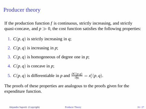
If the production functionf is continuous, strictly increasing, and strictlyquasi-concave, andp ≫ 0, the cost function satisfies the following properties:

1. C(p, q) is strictly increasing inq;

2. C(p, q) is increasing inp;

3. C(p, q) is homogeneous of degree one inp;

4. C(p, q) is concave inp;

5. C(p, q) is differentiable inp and ∂C(p,q)∂pi

= xci (p, q).

The proofs of these properties are analogous to the proofs given for theexpenditure function.


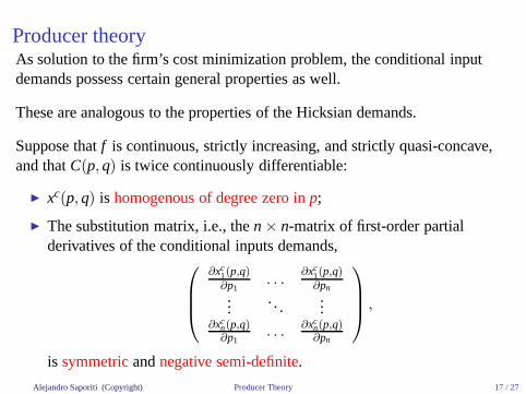
Producer theoryAs solution to the firm’s cost minimization problem, the conditional inputdemands possess certain general properties as well.

These are analogous to the properties of the Hicksian demands.

Suppose thatf is continuous, strictly increasing, and strictly quasi-concave,and thatC(p, q) is twice continuously differentiable:

◮ xc(p, q) is homogenous of degree zero inp;

◮ The substitution matrix, i.e., then × n-matrix of first-order partialderivatives of the conditional inputs demands,

∂xc1(p,q)∂p1

. . .∂xc

1(p,q)∂pn

.... . .

...∂xc

n(p,q)∂p1

. . . ∂xcn(p,q)∂pn

,

is symmetricandnegative semi-definite.


Producer theory

Therefore, by definition of negative semi-definiteness, theelements of thediagonal are non-positive; i.e., for alli = 1, . . . , n,

∂xci (p, q)

∂pi=

∂2C(p, q)

∂p2i

≤ 0. (7)

That means, the conditional input demands cannot have a positive slope!

After a fall in p1, the firm substitutesx2, whose relative price has increased, bythe relatively cheaper inputx1 (law of demand).

The substitution effect is driven by the assumed nature of the technology,namely, by the convexity of the isoquant curves.


Producer theoryFinally, let’s determine the optimal output of thecompetitive firmtomaximize its profits, which amounts to solving

maxq≥0

pq · q − C(p, q), (8)

wherepq is the market price at which the firm sell each unit ofq.

If q∗ > 0 is the solution of (8), then the firm must satisfy the FOC

pq −∂C(p, q∗)

∂q= 0. (9)

That is, the optimal outputq∗ is chosen in such a way that theoutput priceequals the marginal costat q∗!

SOC requires that the marginal cost be nondecreasing atq∗, i.e.,

∂2C(p, q∗)∂q2 ≥ 0.


Producer theoryThe optimal outputq∗ depends on(pq, p). By changing “this data”, we get theoutput supply functionof the competitive firm, denoted byq(pq, p).

Replacingq(pq, p) into the condition input demands, we get theunconditionalinput demandsx(pq, p) = xc(p, q(pq, p)).

Finally, recall that by the Envelope theorem,∂C(p,q)∂q = λ.

Moreover, by the FOC,λ = pi/MPi(x).

Therefore, using (9), it follows that for alli = 1, . . . , n,

pq −pi

MPi(x)= 0 ⇔ pq · MPi(x) = pi. (10)

In words, (10) says that the competitive firm employs additional units of inputi until its marginal revenue product, pq · MPi(x), equals its unit cost,pi.


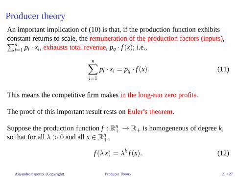
Producer theoryAn important implication of (10) is that, if the production function exhibitsconstant returns to scale, theremuneration of the production factors (inputs),∑n

i=1 pi · xi, exhausts total revenue, pq · f (x); i.e.,

n∑

i=1

pi · xi = pq · f (x). (11)

This means the competitive firm makesin the long-run zero profits.

The proof of this important result rests onEuler’s theorem.

Suppose the production functionf : Rn+ → R+ is homogeneous of degreek,

so that for allλ > 0 and allx ∈ Rn+,

f (λ x) = λk f (x). (12)


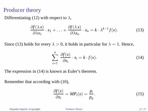
Producer theoryDifferentiating (12) with respect toλ,

∂f (λ x)∂λx1

· x1 + . . . +∂f (λ x)∂λxn

· xn = k · λk−1 f (x). (13)

Since (13) holds for everyλ > 0, it holds in particular forλ = 1. Hence,

n∑

i=1

∂f (x)∂xi

· xi = k · f (x). (14)

The expression in (14) is known as Euler’s theorem.

Remember that according with (10),

∂f (x)∂xi

= MPi(x) =pi

pq. (15)


Producer theory

Therefore, substituting (15) into (14), we have that

n∑

i=1

pi · xi = k · pq · f (x).

Thus, if the production functionf hasconstant returns to scale(i.e., if k = 1),then we have that in the equilibrium of the competitive firm:

n∑

i=1

pi · xi = pq · f (x),

which is exactly the expression in (11).


Producer theory

Themaximum-value function of the profit functiondepends on input andoutput prices and is defined as follows:

π(pq, p) = max(x,q)∈R

n+1+

{

pq q −

n∑

i=1

pi xi : f (x1, . . . , xn) ≥ q

}

. (16)

It is easy to see thatπ(pq, p) is well defined only if the production functiondoesn’t exhibit increasing returns to scale.

On the contrary, supposef has increasing RS, and letx∗ andq∗ = f (x∗)maximizeπ at pricespq andp = (p1, . . . , pn).


Producer theory

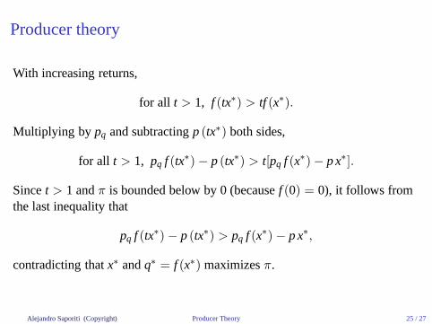
With increasing returns,

for all t > 1, f (tx∗) > tf (x∗).

Multiplying by pq and subtractingp (tx∗) both sides,

for all t > 1, pq f (tx∗) − p (tx∗) > t[pq f (x∗) − p x∗].

Sincet > 1 andπ is bounded below by 0 (becausef (0) = 0), it follows fromthe last inequality that

pq f (tx∗) − p (tx∗) > pq f (x∗) − p x∗,

contradicting thatx∗ andq∗ = f (x∗) maximizesπ.


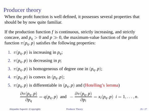
Producer theoryWhen the profit function is well defined, it possesses severalproperties thatshould be by now quite familiar.

If the production functionf is continuous, strictly increasing, and strictlyconcave, andpq > 0 andp ≫ 0, the maximum-value function of the profitfunctionπ(pq, p) satisfies the following properties:

1. π(pq, p) is increasing inpq;

2. π(pq, p) is decreasing inp;

3. π(pq, p) is homogeneous of degree one in(pq, p);

4. π(pq, p) is convex in(pq, p);

5. π(pq, p) is differentiable in(pq, p) and (Hotelling’s lemma)

∂π(pq, p)

∂pq= q(pq, p) and −

∂π(pq, p)

∂pi= xi(pq, p) i = 1, . . . , n.


Producer theory

In particular, the fact thatπ(pq, p) is convex in(pq, p) implies that the Hessianof π(·) is positive semi-definite.

Therefore, all of the elements in the main diagonal are nonnegative, i.e.,

∂2π(pq, p)

∂p2q

=∂q(pq, p)

∂pq≥ 0,

and

−∂2π(pq, p)

∂p2i

=∂xi(pq, p)

∂pi≤ 0 for all i = 1, . . . , n.

In words, the output supplyq(pq, p) is increasing in the product pricepq, andthe input demandsxi(pq, p) are decreasing in their own input pricepi.


notes on producer theory - university of...

Documents