novel techniques for e cient and e ective subgroup discovery
TRANSCRIPT

Novel Techniques for
Efficient and Effective Subgroup Discovery
vorgelegt von
Florian Lemmerich
Dissertation zur Erlangung des naturwissenschaftlichen Doktorgrades
der Bayerischen Julius-Maximilians-Universitat Wurzburg


AbstractLarge volumes of data are collected today in many domains. Often, there is so much dataavailable, that it is difficult to identify the relevant pieces of information. Knowledgediscovery seeks to obtain novel, interesting and useful information from large datasets.One key technique for that purpose is subgroup discovery. It aims at identifying de-scriptions for subsets of the data, which have an interesting distribution with respectto a predefined target concept. This work improves the efficiency and effectiveness ofsubgroup discovery in different directions.
For efficient exhaustive subgroup discovery, algorithmic improvements are proposedfor three important variations of the standard setting: First, novel optimistic estimatebounds are derived for subgroup discovery with numeric target concepts. These allow forskipping the evaluation of large parts of the search space without influencing the results.Additionally, necessary adaptations to data structures for this setting are discussed.Second, for exceptional model mining, that is, subgroup discovery with a model overmultiple attributes as target concept, a generic extension of the well-known FP-tree datastructure is introduced. The modified data structure stores intermediate condensed datarepresentations, which depend on the chosen model class, in the nodes of the trees. Thisallows the application for many popular model classes. Third, subgroup discovery withgeneralization-aware measures is investigated. These interestingness measures comparethe target share or mean value in the subgroup with the respective maximum value inall its generalizations. For this setting, a novel method for deriving optimistic estimatesis proposed. In contrast to previous approaches, the novel measures are not exclusivelybased on the anti-monotonicity of instance coverage, but also takes the difference ofcoverage between the subgroup and its generalizations into account. In all three areas,the advances lead to runtime improvements of more than an order of magnitude.
The second part of the contributions focuses on the effectiveness of subgroup discovery.These improvements aim to identify more interesting subgroups in practical applications.For that purpose, the concept of expectation-driven subgroup discovery is introduced asa new family of interestingness measures. It computes the score of a subgroup based onthe difference between the actual target share and the target share that could be expectedgiven the statistics for the separate influence factors that are combined to describe thesubgroup. In doing so, previously undetected interesting subgroups are discovered, whileother, partially redundant findings are suppressed.
Furthermore, this work also approaches practical issues of subgroup discovery: In thatdirection, the VIKAMINE 2 tool is presented, which extends its predecessor with a re-build user interface, novel algorithms for automatic discovery, new interactive miningtechniques, as well novel options for result presentation and introspection. Finally, somereal-world applications are described that utilized the presented techniques. These in-clude the identification of influence factors on the success and satisfaction of universitystudents and the description of locations using tagging data of geo-referenced images.
i


Acknowledgements
This work was supported by many people: First of all, I want to thank my supervisorFrank Puppe for all the open-minded discussions, his always open door, and for pro-viding a great and enjoyable research environment. In addition, I would like to offer myspecial thanks to Martin Atzmueller and Andreas Hotho for their guidance, expertiseand feedback.
Many thanks to my colleagues and friends at our working group, who helped mewith countless technical, organizational and scientific issues: Alexander Hornlein, BeateNavarro Bullock, Daniel Zoller, Georg Dietrich, Georg Fette, Joachim Baumeister,Jochen Reutelshofer, Lena Schwemmlein, Marianus Ifland, Martin Becker, MartinToepfer, Peter Klugl, Petra Braun, Philip-Daniel Beck, Reinhard Hatko, and ThomasNiebler.
I also want to thank my reviewers Arno Knobbe from the Universiteit Leiden, andNada Lavrac from the Jozef Stefan Institute Ljubljana, who accompanied my scientificjourney from my first international workshop to the final weeks of this thesis.
I dedicate this work to my family. They provided me the anchor for my life and never-ending encouragement on my way. Most of all, this is for my wife Eva-Maria, who wentwith me through ups and downs. We’ve made it!
Wurzburg, December 2013 / May 2014
iii

Contents
1 Introduction 11.1 Motivation . . . . . . . . . . . . . . . . . . . . . . . . . . . . . . . . . . . 1
1.2 Goal . . . . . . . . . . . . . . . . . . . . . . . . . . . . . . . . . . . . . . . 2
1.3 Contributions . . . . . . . . . . . . . . . . . . . . . . . . . . . . . . . . . . 3
1.4 Structure of the Work . . . . . . . . . . . . . . . . . . . . . . . . . . . . . 5
2 The Subgroup Discovery Problem 72.1 Definition of Subgroup Discovery . . . . . . . . . . . . . . . . . . . . . . . 7
2.2 Dataset . . . . . . . . . . . . . . . . . . . . . . . . . . . . . . . . . . . . . 8
2.3 Search Space . . . . . . . . . . . . . . . . . . . . . . . . . . . . . . . . . . 8
2.3.1 Nominal Attributes . . . . . . . . . . . . . . . . . . . . . . . . . . . 9
2.3.2 Numeric Attributes . . . . . . . . . . . . . . . . . . . . . . . . . . . 10
2.4 Target Concept . . . . . . . . . . . . . . . . . . . . . . . . . . . . . . . . . 13
2.4.1 Binary Target Concepts . . . . . . . . . . . . . . . . . . . . . . . . 13
2.4.2 Numeric Target Concepts . . . . . . . . . . . . . . . . . . . . . . . 13
2.4.3 Complex Target Concepts . . . . . . . . . . . . . . . . . . . . . . . 14
2.5 Selection Criteria . . . . . . . . . . . . . . . . . . . . . . . . . . . . . . . . 14
2.5.1 Criteria for Interestingness . . . . . . . . . . . . . . . . . . . . . . 15
2.5.2 Interestingness Measures versus Constraints . . . . . . . . . . . . . 16
2.5.3 Interestingness Measures . . . . . . . . . . . . . . . . . . . . . . . . 17
2.5.3.1 Order Equivalence . . . . . . . . . . . . . . . . . . . . . . 18
2.5.3.2 Interestingness Measures for Binary Target Concepts . . 18
2.5.3.3 Interestingness Measures for Numeric Target Concepts . 21
2.5.3.4 Interestingness Measures for Complex Target Concepts . 27
2.5.4 Generalization-Awareness . . . . . . . . . . . . . . . . . . . . . . . 29
2.5.5 Avoiding Redundancy . . . . . . . . . . . . . . . . . . . . . . . . . 30
2.5.5.1 Covering Approaches . . . . . . . . . . . . . . . . . . . . 31
2.5.5.2 Filtering Irrelevant Subgroups . . . . . . . . . . . . . . . 31
2.5.5.3 Subgroup Set Mining . . . . . . . . . . . . . . . . . . . . 32
2.5.5.4 Clustering of Results . . . . . . . . . . . . . . . . . . . . 33
2.6 Background Knowledge . . . . . . . . . . . . . . . . . . . . . . . . . . . . 33
2.7 The Interactive Subgroup Discovery Process . . . . . . . . . . . . . . . . . 34
2.8 Complexity of the Subgroup Discovery Task . . . . . . . . . . . . . . . . . 36
2.9 Statistical Significance of Results . . . . . . . . . . . . . . . . . . . . . . . 37
2.10 Subgroup Discovery and Other Data Mining Tasks . . . . . . . . . . . . . 39
2.10.1 Other Techniques for Supervised Descriptive Pattern Mining . . . 40
v

Contents
2.10.2 Classification . . . . . . . . . . . . . . . . . . . . . . . . . . . . . . 412.10.3 Association Rule Mining . . . . . . . . . . . . . . . . . . . . . . . . 422.10.4 Clustering . . . . . . . . . . . . . . . . . . . . . . . . . . . . . . . . 42
2.11 Overview of Notations . . . . . . . . . . . . . . . . . . . . . . . . . . . . . 432.12 Summary . . . . . . . . . . . . . . . . . . . . . . . . . . . . . . . . . . . . 43
3 Subgroup Discovery Algorithms 453.1 Algorithmic Components . . . . . . . . . . . . . . . . . . . . . . . . . . . 463.2 Enumeration Strategies . . . . . . . . . . . . . . . . . . . . . . . . . . . . 46
3.2.1 Depth-first-search and Variants . . . . . . . . . . . . . . . . . . . . 473.2.2 Levelwise Approaches . . . . . . . . . . . . . . . . . . . . . . . . . 523.2.3 Best-first-search . . . . . . . . . . . . . . . . . . . . . . . . . . . . 533.2.4 Beam-search . . . . . . . . . . . . . . . . . . . . . . . . . . . . . . 543.2.5 Genetic Algorithms . . . . . . . . . . . . . . . . . . . . . . . . . . . 55
3.3 Data Structures . . . . . . . . . . . . . . . . . . . . . . . . . . . . . . . . . 563.3.1 Basic Data Storage . . . . . . . . . . . . . . . . . . . . . . . . . . . 563.3.2 Vertical Data Structures . . . . . . . . . . . . . . . . . . . . . . . . 563.3.3 FP-tree Structures and Derivates . . . . . . . . . . . . . . . . . . . 58
3.4 Pruning Strategies . . . . . . . . . . . . . . . . . . . . . . . . . . . . . . . 613.4.1 Anti-monotone Constraints . . . . . . . . . . . . . . . . . . . . . . 623.4.2 Optimistic Estimate Pruning . . . . . . . . . . . . . . . . . . . . . 633.4.3 Optimistic Estimates for Common Binary Interestingness Measures 64
3.5 Algorithms . . . . . . . . . . . . . . . . . . . . . . . . . . . . . . . . . . . 653.5.1 Explora . . . . . . . . . . . . . . . . . . . . . . . . . . . . . . . . . 663.5.2 MIDOS . . . . . . . . . . . . . . . . . . . . . . . . . . . . . . . . . 663.5.3 The CN2 Family . . . . . . . . . . . . . . . . . . . . . . . . . . . . 663.5.4 OPUS . . . . . . . . . . . . . . . . . . . . . . . . . . . . . . . . . . 673.5.5 SD . . . . . . . . . . . . . . . . . . . . . . . . . . . . . . . . . . . . 673.5.6 STUCCO . . . . . . . . . . . . . . . . . . . . . . . . . . . . . . . . 673.5.7 Apriori-C and Apriori-SD . . . . . . . . . . . . . . . . . . . . . . . 673.5.8 Apriori SMP . . . . . . . . . . . . . . . . . . . . . . . . . . . . . . 683.5.9 Harmony . . . . . . . . . . . . . . . . . . . . . . . . . . . . . . . . 683.5.10 CorClass and CG . . . . . . . . . . . . . . . . . . . . . . . . . . . . 683.5.11 Corrmine . . . . . . . . . . . . . . . . . . . . . . . . . . . . . . . . 683.5.12 SDIGA and MESDIF . . . . . . . . . . . . . . . . . . . . . . . . . 693.5.13 Algorithm of Cerf . . . . . . . . . . . . . . . . . . . . . . . . . . . 693.5.14 CCCS . . . . . . . . . . . . . . . . . . . . . . . . . . . . . . . . . . 693.5.15 CMAR . . . . . . . . . . . . . . . . . . . . . . . . . . . . . . . . . 693.5.16 SD-Map . . . . . . . . . . . . . . . . . . . . . . . . . . . . . . . . . 693.5.17 DpSubgroup . . . . . . . . . . . . . . . . . . . . . . . . . . . . . . 703.5.18 DDPMine . . . . . . . . . . . . . . . . . . . . . . . . . . . . . . . . 703.5.19 Overview of Algorithms . . . . . . . . . . . . . . . . . . . . . . . . 70
3.6 Algorithms for Special Cases . . . . . . . . . . . . . . . . . . . . . . . . . 703.6.1 Algorithms for Relevant Subgroups . . . . . . . . . . . . . . . . . . 70
vi

Contents
3.6.2 Numeric Selectors . . . . . . . . . . . . . . . . . . . . . . . . . . . 72
3.6.3 Large Scale Mining Adaptations . . . . . . . . . . . . . . . . . . . 73
3.6.3.1 Sampling . . . . . . . . . . . . . . . . . . . . . . . . . . . 73
3.6.3.2 Parallelization . . . . . . . . . . . . . . . . . . . . . . . . 74
3.7 Summary . . . . . . . . . . . . . . . . . . . . . . . . . . . . . . . . . . . . 75
4 Algorithms for Numeric Target Concepts 774.1 Related Work . . . . . . . . . . . . . . . . . . . . . . . . . . . . . . . . . . 78
4.2 Optimistic Estimates . . . . . . . . . . . . . . . . . . . . . . . . . . . . . . 79
4.2.1 Differences to the Binary Setting . . . . . . . . . . . . . . . . . . . 80
4.2.2 Optimistic Estimates with Closed Form Expressions . . . . . . . . 81
4.2.2.1 Mean-based Interestingness Measures . . . . . . . . . . . 81
4.2.2.2 Median-based Measures . . . . . . . . . . . . . . . . . . . 86
4.2.2.3 (Full) Distribution-based Measures . . . . . . . . . . . . . 86
4.2.2.4 Rank-based Measures . . . . . . . . . . . . . . . . . . . . 88
4.2.3 Ordering-based Bounds . . . . . . . . . . . . . . . . . . . . . . . . 89
4.2.3.1 One-pass Estimates by Ordering . . . . . . . . . . . . . . 89
4.2.3.2 Two-pass Estimates by Ordering . . . . . . . . . . . . . . 91
4.2.3.3 Interestingness Measures not Estimable by Ordering . . . 92
4.2.4 Fast Bounds using Limited Information . . . . . . . . . . . . . . . 93
4.3 Data Representations . . . . . . . . . . . . . . . . . . . . . . . . . . . . . 95
4.3.1 Adaptations of FP-trees . . . . . . . . . . . . . . . . . . . . . . . . 96
4.3.2 Adaptation of Bitset-based Data Structures . . . . . . . . . . . . . 97
4.4 Algorithms for Subgroup Discovery with Numeric Targets . . . . . . . . . 98
4.4.1 The SD-Map* Algorithm . . . . . . . . . . . . . . . . . . . . . . . 98
4.4.2 The NumBSD Algorithm . . . . . . . . . . . . . . . . . . . . . . . 99
4.5 Evaluation . . . . . . . . . . . . . . . . . . . . . . . . . . . . . . . . . . . . 101
4.5.1 Effects of Optimistic Estimates . . . . . . . . . . . . . . . . . . . . 101
4.5.2 Influence of the Result Set Size . . . . . . . . . . . . . . . . . . . . 106
4.5.3 Influences of Data Structures . . . . . . . . . . . . . . . . . . . . . 106
4.5.4 Runtimes of the Full Algorithms . . . . . . . . . . . . . . . . . . . 109
4.5.5 Effects of the Fast Pruning Bounds . . . . . . . . . . . . . . . . . . 114
4.5.6 Evaluation Summary . . . . . . . . . . . . . . . . . . . . . . . . . . 114
4.6 Overview of Computational Properties of Interestingness Measures . . . . 115
4.7 Summary . . . . . . . . . . . . . . . . . . . . . . . . . . . . . . . . . . . . 116
4.8 Appendix . . . . . . . . . . . . . . . . . . . . . . . . . . . . . . . . . . . . 117
5 Efficient Exhaustive Exceptional Model Mining through Generic Pattern Trees 1195.1 Related Work . . . . . . . . . . . . . . . . . . . . . . . . . . . . . . . . . . 120
5.2 GP-growth . . . . . . . . . . . . . . . . . . . . . . . . . . . . . . . . . . . 121
5.2.1 The Concept of Valuation Bases . . . . . . . . . . . . . . . . . . . 121
5.2.2 Algorithmic Adaptations . . . . . . . . . . . . . . . . . . . . . . . 123
5.3 Theorem on Condensed Valuation Bases . . . . . . . . . . . . . . . . . . . 125
vii

Contents
5.4 Valuation Bases for Important Model Classes . . . . . . . . . . . . . . . . 126
5.4.1 Variance Model . . . . . . . . . . . . . . . . . . . . . . . . . . . . . 126
5.4.2 Correlation Model . . . . . . . . . . . . . . . . . . . . . . . . . . . 127
5.4.3 Linear Regression Model . . . . . . . . . . . . . . . . . . . . . . . . 130
5.4.4 Logistic Regression Model . . . . . . . . . . . . . . . . . . . . . . . 130
5.4.5 DTM-Classifier . . . . . . . . . . . . . . . . . . . . . . . . . . . . . 131
5.4.6 Accuracy of Classifiers . . . . . . . . . . . . . . . . . . . . . . . . . 132
5.4.7 Bayesian Networks . . . . . . . . . . . . . . . . . . . . . . . . . . . 132
5.5 Evaluation . . . . . . . . . . . . . . . . . . . . . . . . . . . . . . . . . . . . 132
5.5.1 Runtime Evaluations on UCI data . . . . . . . . . . . . . . . . . . 132
5.5.2 Scalability Study: Social Image Data . . . . . . . . . . . . . . . . . 136
5.6 Summary . . . . . . . . . . . . . . . . . . . . . . . . . . . . . . . . . . . . 136
6 Difference-based Estimates for Generalization-Aware Subgroup Discovery 1376.1 Related Work . . . . . . . . . . . . . . . . . . . . . . . . . . . . . . . . . . 138
6.2 Estimates for Generalization-Aware Subgroup Mining . . . . . . . . . . . 139
6.2.1 Optimistic Estimates Based on Covered Positive Instances . . . . . 139
6.2.2 Difference-based Pruning . . . . . . . . . . . . . . . . . . . . . . . 141
6.2.3 Difference-based Optimistic Estimates for Binary Targets . . . . . 142
6.2.4 Difference-based Optimistic Estimates for Numeric Targets . . . . 146
6.3 Algorithm . . . . . . . . . . . . . . . . . . . . . . . . . . . . . . . . . . . . 147
6.4 Evaluation . . . . . . . . . . . . . . . . . . . . . . . . . . . . . . . . . . . . 149
6.5 Summary . . . . . . . . . . . . . . . . . . . . . . . . . . . . . . . . . . . . 153
7 Local Models for Expectation-Driven Subgroup Discovery 1557.1 Approach and Motivation . . . . . . . . . . . . . . . . . . . . . . . . . . . 155
7.2 Related Work . . . . . . . . . . . . . . . . . . . . . . . . . . . . . . . . . . 157
7.3 A Generalized Approach on the Subgroup Discovery Task . . . . . . . . . 159
7.4 Expectations Through Bayesian Network Fragments . . . . . . . . . . . . 160
7.5 Expectations for Influence Combination . . . . . . . . . . . . . . . . . . . 162
7.5.1 Classic Subgroup Discovery . . . . . . . . . . . . . . . . . . . . . . 162
7.5.2 Minimum Improvement . . . . . . . . . . . . . . . . . . . . . . . . 162
7.5.3 Leaky-Noisy-Or . . . . . . . . . . . . . . . . . . . . . . . . . . . . . 162
7.5.4 Additive Synergy and Multiplicative Synergy . . . . . . . . . . . . 163
7.5.5 Logit-Model . . . . . . . . . . . . . . . . . . . . . . . . . . . . . . . 164
7.6 Computational Aspects of Mining Unexpected Patterns . . . . . . . . . . 164
7.7 Evaluation . . . . . . . . . . . . . . . . . . . . . . . . . . . . . . . . . . . . 165
7.7.1 Experiments with Public Data . . . . . . . . . . . . . . . . . . . . 165
7.7.2 Values for Expectation Functions . . . . . . . . . . . . . . . . . . . 168
7.7.3 Case Study: Educational Domain . . . . . . . . . . . . . . . . . . . 168
7.7.4 Case Study: Spammer Domain . . . . . . . . . . . . . . . . . . . . 171
7.8 Discussion and Possible Improvements . . . . . . . . . . . . . . . . . . . . 174
7.9 Summary . . . . . . . . . . . . . . . . . . . . . . . . . . . . . . . . . . . . 175
viii

Contents
8 VIKAMINE 2: A Flexible Subgroup Discovery Tool 1778.1 VIKAMINE 2 : Overview . . . . . . . . . . . . . . . . . . . . . . . . . . . 1788.2 Architecture . . . . . . . . . . . . . . . . . . . . . . . . . . . . . . . . . . . 1798.3 An Extensible User Interface . . . . . . . . . . . . . . . . . . . . . . . . . 1798.4 Handling of Numeric Attributes . . . . . . . . . . . . . . . . . . . . . . . . 1818.5 A Scalable View for Interactive Mining . . . . . . . . . . . . . . . . . . . . 1818.6 Result Presentation . . . . . . . . . . . . . . . . . . . . . . . . . . . . . . . 183
8.6.1 Pie Circle Visualization . . . . . . . . . . . . . . . . . . . . . . . . 1848.6.2 Subgroup Treetable . . . . . . . . . . . . . . . . . . . . . . . . . . 186
8.7 A Framework for Textual Acquisition of Background Knowledge . . . . . 1878.8 Integrated Exploratory Data Analysis with EDAT . . . . . . . . . . . . . 1898.9 Summary . . . . . . . . . . . . . . . . . . . . . . . . . . . . . . . . . . . . 190
9 Applications: Case Studies in Subgroup Discovery 1939.1 Students’ Success and Satisfaction . . . . . . . . . . . . . . . . . . . . . . 193
9.1.1 Dropout Analysis . . . . . . . . . . . . . . . . . . . . . . . . . . . . 1949.1.2 Indicators for Thesis Grades . . . . . . . . . . . . . . . . . . . . . . 1959.1.3 A Survey Analysis on Student Satisfaction . . . . . . . . . . . . . . 197
9.1.3.1 Dataset . . . . . . . . . . . . . . . . . . . . . . . . . . . . 1979.1.3.2 Influence Factors for the Overall Satisfaction . . . . . . . 1979.1.3.3 Gender Diversity in Student Satisfaction . . . . . . . . . 199
9.1.4 Case Study Summary . . . . . . . . . . . . . . . . . . . . . . . . . 2009.2 Mining Patterns in Geo-referenced Social Media Data . . . . . . . . . . . 201
9.2.1 Dataset . . . . . . . . . . . . . . . . . . . . . . . . . . . . . . . . . 2019.2.2 Automatic Techniques . . . . . . . . . . . . . . . . . . . . . . . . . 202
9.2.2.1 Target Concept Construction . . . . . . . . . . . . . . . . 2029.2.2.2 Avoiding User Bias: User–Resource Weighting . . . . . . 203
9.2.3 Visualization . . . . . . . . . . . . . . . . . . . . . . . . . . . . . . 2049.2.4 Application Example: Berlin Area . . . . . . . . . . . . . . . . . . 2049.2.5 Case Study Summary . . . . . . . . . . . . . . . . . . . . . . . . . 206
9.3 Pattern Mining for Improved Conditional Random Fields . . . . . . . . . 2079.4 CaseTrain . . . . . . . . . . . . . . . . . . . . . . . . . . . . . . . . . . . . 2099.5 Industrial Application . . . . . . . . . . . . . . . . . . . . . . . . . . . . . 2109.6 I-Pat Challenge . . . . . . . . . . . . . . . . . . . . . . . . . . . . . . . . . 2119.7 Discussion . . . . . . . . . . . . . . . . . . . . . . . . . . . . . . . . . . . . 2119.8 Summary . . . . . . . . . . . . . . . . . . . . . . . . . . . . . . . . . . . . 212
10 Conclusions 21310.1 Summary . . . . . . . . . . . . . . . . . . . . . . . . . . . . . . . . . . . . 21310.2 Outlook . . . . . . . . . . . . . . . . . . . . . . . . . . . . . . . . . . . . . 215
Appendix: Bibliography 217
ix


1 Introduction
1.1 Motivation
“It’s a very sad thing that nowadays there is so little useless information.”1 As thisquote of Oscar Wilde shows, information was a valuable commodity already more thanone century ago. Almost each piece of data seemed to be potentially beneficial alreadyin these times. In the last decades, the significance of information in our society onlyincreased further, and it increased rapidly. In fact, it increased so much that some call thecurrent period of human history the information age. Massive amounts of informationare collected and stored every day in the most diverse domains. However, this abundanceof information also has its downsides: “What information consumes is rather obvious: itconsumes the attention of its recipients. Hence, a wealth of information creates a povertyof attention and a need to allocate that attention efficiently among the overabundanceof information sources that might consume it.”2 This expresses a common concern:There is so much raw information available that it gets difficult to extract relevantand interesting knowledge. To support this course of action with current computertechnology, the research field of knowledge discovery in databases has been establishedin order “to assist humans in extracting useful information (knowledge) from the rapidlygrowing volumes of digital data” [80].
For knowledge discovery in databases, a diverse set of methods has been proposed inthe last decades. One of the key techniques is subgroup discovery. Subgroup discoveryaims at finding descriptions of subsets of the data instances that show an interestingdistribution with respect to a predefined target concept. It is a descriptive and supervisedtechnique. Descriptive means that results are directly interpretable by human experts.Supervised expresses that the user specifies a certain property of interest, which is thefocus of the knowledge discovery process.
Consider as an illustrating example a dataset from the medical domain: The datainstances are given by a large set of patients with a certain disease. For each patienta variety of information is provided, e.g., age, gender, measurements about the currentmedical condition, and previous diseases. Furthermore it is known for each patient ifthe treatment with a certain drug was successful or not. This information is of specificinterest and is thus used as the target concept for subgroup discovery. Assume thatthe treatment was overall successful in 30% of the cases. Then, one can speculate thatthere are some groups of patients, for which the treatment is especially well suited. Forthese patients, the treatment should have a higher success rate. For example, one could
1Wilde, Oscar: A Few Maxims For The Instruction Of The Over-Educated, Saturday Review, 1894.2Simon, Herbert A., Designing Organizations for an Information-Rich World, in: Greenberger, Martin,
Computers, Communication, and the Public Interest, The Johns Hopkins Press, 1971.
1

1 Introduction
hypothesize that the treatment is in particular successful for young, female patientswith high blood pressure. For each conjunction of selection expressions (e.g., gender isfemale AND age is young AND blood pressure is high), one hypothesis about the effectof the treatment in this group of people can be formed. Unfortunately, given a largeset of describing properties, there is a huge set of possible conjunctive combinations.Therefore, it is clearly intractable to report the statistics for all possible hypotheses to ahuman expert. Instead, an automatic subgroup discovery algorithm can be used to selectsubgroups, which are supposedly interesting for humans, e.g., because the success rate ofthe treatment is significantly increased or decreased. Thus, one relevant finding identifiedby subgroup discovery could be stated as “While the success rate of the treatment wasonly at 30 % of all cases, for the 30 young, female patients with high blood pressure,the success rate was at 75%.” Such findings are usually identified by performing asearch through the set of candidate hypotheses and score each of them with a value thatrates its supposed interestingness. In addition to this purely automatic approach, theinvolvement of human experts is favorable in order to guide the search in an iterative andinteractive approach. This example used a binary property as the target concept (thetreatment is either successful or not), but variations of subgroup discovery also employnumeric properties or even complex models over multiple attributes as target concepts.
Subgroup discovery is an established technique that has been successfully applied innumerous practical applications. Nonetheless, it still provides diverse challenges, whichwill be approached in this work.
1.2 Goal
The main challenges in the research on subgroup discovery, can be distinguished intotwo different categories:
The first type is concerned with the efficiency of discovery algorithms. In order toidentify interesting patterns, a large number of candidates has to be evaluated. That is,the number of subgroup evaluations is high-order polynomial or even exponential (de-pending on the applied constraints) with respect to the number of selection expressionsallowed to describe the subgroup. Therefore, fast algorithms are key in order to handlelarge-scale applications. However, the speed of subgroup discovery algorithms is not onlyan issue for large datasets. Since subgroup discovery involves an iterative and interactiveprocess, automatic discovery is often executed repeatedly with slightly modified settingsby a domain expert with limited time for the analysis. In such a scenario, the reductionof runtime from a few minutes to a few seconds can substantially improve the user expe-rience. The efficiency of algorithms is well explored in the standard subgroup discoverysetting with binary target concepts and simple interestingness measures. However, forvariations of this task fast algorithms are yet to be developed, e.g., for subgroup discov-ery with a numeric target concept, for exceptional model mining (subgroup discoverywith multiple target attributes) and for generalization-aware interestingness measures.This work aims at providing novel techniques that enable efficient subgroup discoveryalso in these more complex settings. In these directions, in particular exhaustive mining
2

1.3 Contributions
techniques are explored, which can guarantee that the optimal results are returned withrespect to the employed selection criteria.
The second type of challenges relates to the effectiveness of subgroup discovery. Thisdescribes that the discovered patterns are close to what is actually interesting or usefulin real-world applications. One problem in particular is that results from automaticalgorithms are often redundant, that is, they can be expected with respect to otherfindings, especially to more general subgroup descriptions. Since often only the top (e.g.,the top 20) subgroups are presented to human experts, other, potentially interestingsubgroups are not displayed in favor of these redundant findings. In that direction, thiswork seeks to find novel selection criteria to improve the quality of subgroup discoveryresults. Finally, the introduced techniques should also be available for interactive realworld-applications.
1.3 Contributions
The first part of the contribution focuses on the efficiency of automatic discovery algo-rithms. That is, the same subgroups as in previous approaches are discovered, but insubstantially less time:
In that direction, algorithms for fast subgroup discovery from literature are reviewedin detail. Instead of describing the algorithms one-by-one, improvements are categorizedin three dimensions, that is, the strategies for candidate enumeration, the utilized datastructures and the applied pruning strategies, which allow skipping parts of the evalua-tion without affecting the results. Algorithmic components for all three dimensions arediscussed in detail. This allows describing actual algorithms concisely in terms of thethree dimensions. The summary of related work is not exclusively focused on subgroupdiscovery algorithms, but also references contributions from related fields, even if thesediffer in the applied terminology or specific goal.
The first set of novel techniques is concerned with subgroup discovery with a numerictarget concept. For this task, optimistic estimate bounds are developed for a large varietyof interestingness measures. Applying these optimistic estimate bounds allows to prunelarge parts of the search space while maintaining the optimality of results. For someof the bounds closed form expressions, which are based on a few key statistics, canbe determined. This is required for algorithms that use FP-tree-based data structures.Other, ordering-based optimistic estimates can be derived by checking multiple subsets ofthe subgroup’s instances. While the computation of these bounds requires a full pass overall instance for each subgroup, it results in tighter bounds. Additionally, the adaptationof two different data structures to the numeric target setting is presented, that is, FP-trees and bitset-based data representations. Two novel algorithms implement theseimprovements: The SD-Map* algorithm utilizes adapted FP-trees as data structures andoptimistic estimates in closed form. The NumBSD algorithm exploits bitset-based datastructures and ordering-based optimistic estimate bounds. Experimental evaluationsshow that both outperform previous approaches by an order of magnitude.
3

1 Introduction
Another contribution focuses on the extension of the FP-tree data structure to thearea of exceptional model mining. This extension of classical subgroup discovery usesa model over multiple attributes instead of a single attribute as target concept. Sincedifferent model classes have heterogeneous computational requirements, a generic datastructure is necessary. For that purpose, the concept of valuation bases is introduced asan intermediate condensed data representation. While the structure of the FP-tree ismaintained, the information that is stored in each tree node is replaced by a valuationbasis depending on the model classes. This approach is suited for many, but not all modelclasses. A concise characterization of applicable model classes is provided by drawing ananalogy to parallel data stream mining. Furthermore, examples of valuation bases arepresented for many model classes. The implementation of the novel data structure ina new algorithm called GP-growth leads to massive speed-ups in comparison to a naiveexhaustive depth-first search.
Generalization-aware interestingness measures improve traditional selection criteriafor subgroup discovery by comparing the statistics of a subgroup not only to the statis-tics of the overall population, but also to the statistics of all its generalizations. In doingso, redundant findings are avoided and more interesting subgroups are discovered. Forimproved efficiency of subgroup discovery with these measures, a novel method of de-riving optimistic estimates bounds is introduced. Unlike previous approaches, the noveloptimistic estimates are not only based on the anti-monotonicity of instance coverage,but also take into account the difference of the coverage between a subgroup and its gen-eralizations. Incorporating the new optimistic estimates in state-of-the-art algorithmsimproves the runtime requirements by more than an order of magnitude in many cases.
The second part of the contributions focuses on the effectiveness of subgroup discov-ery. These improvements focus on identifying more interesting subgroups in practicalapplications. In that direction, the concept of expectation-driven subgroup discovery isintroduced. This variant employs a novel family of interestingness measures, which aimsat more interesting subgroup discovery results. It assumes that the statistics for de-scribing basic influence factors imply expectations on the statistics of complex patternswith conjunctive descriptions. The interestingness of a subgroup is then determined bythe difference between the expected and the actual share of the target concept in thesubgroup. A formal computation of expectation values is difficult, as expectations areinherently subjective. For this task, it is shown how established modeling techniques,such as the leaky-noisy-or model, can be transferred from the research of bayesian net-work construction. Several experiments including two real-world case studies demon-strate that the novel techniques detect qualitatively different patterns in comparison topreviously proposed interestingness measures. New, previously undetected interestingsubgroups are discovered, while other, partially redundant findings are suppressed.
The above mentioned core contributions are concerned with more theoretical, butgenerally applicable improvements. Further contributions focus on practical issues ofsubgroup discovery: Since subgroup discovery is not a purely automatic task, but aniterative and interactive process, proper tool support is required. For that purpose, thetool VIKAMINE 2 is presented. VIKAMINE 2 was developed in the context of thiswork, significantly improving and extending its predecessor VIKAMINE in different di-
4

1.4 Structure of the Work
rections. As core component, it provides a broad collection of state-of-the-art algorithmsand interestingness measures for binary as well as numeric target concepts. Automaticand interactive mining options are accessible in a new, appealing graphical user interface,which enables easy extensibility by using the Eclipse RCP-framework. It also featuresnovel techniques for interactive mining in large datasets, the effective presentation ofresults and the introspection of subgroups.
Finally, some real-world applications are presented, which did benefit from the pro-posed novel techniques. A long-term project in the educational domain applied subgroupdiscovery in order to identify influence factors, which affect the success and the satisfac-tion of university students. Another case study showed how techniques from subgroupdiscovery can be adapted for the analysis of geo-referenced tagging data. In this di-rection, meta-data from the Flickr platform could be utilized to obtain descriptions forspecific geographic locations. Further application examples included pattern mining forimproved information extraction with conditional random fields, an industrial applica-tion that was concerned with the fault rate of products, and a challenge dataset regardinggene data analysis.
1.4 Structure of the Work
The remainder of this work is structured in nine chapters, which are to a high degreeself-contained and intelligible in themselves:
Chapters 2 and 3 review previous research on subgroup discovery. Chapter 2 dis-cusses the fundamentals of subgroup discovery, such as possible selection criteria, as wellas general issues, e.g., process models or the statistical significance of discoveries. Chap-ter 3 focuses on algorithmic approaches from literature. In that direction, it discussesenumeration strategies, data structures, and pruning strategies in detail and provides anoverview on previously presented algorithms.
Chapters 4 to 7 present the main theoretical contributions of this work: Chapter 4 in-troduces novel techniques for subgroup discovery with numeric target concepts, i.e., newoptimistic estimate bounds for advanced pruning of the search space and the adaptionof data structures to the numeric target setting. Chapter 5 focuses on exceptional modelmining, that is, subgroup discovery with a model over multiple attributes as target con-cept. In this direction, it is shown how the well-known FP-tree data structure can beadapted for this setting, and for which model classes this can be accomplished. Chapter6 presents difference-based estimates as a novel, generic scheme for optimistic estimatepruning, which can be applied for subgroup discovery with generalization-aware interest-ingness measures. In contrast to these efficiency improvements, Chapter 7 is concernedwith the effectiveness of subgroup discovery. For that purpose, a novel class of interest-ingness measures, that is, expectation-driven interestingness measures, is introduced.
Chapter 8 and Chapter 9 discuss practical issues of subgroup discovery: Chapter 8presents the interactive subgroup discovery tool VIKAMINE 2, while Chapter 9 reportson some successful real-world applications of subgroup discovery.
Finally, Chapter 10 concludes the work with a summary of results and an outlook onfuture work.
5


2 The Subgroup Discovery Problem
This chapter provides a general overview on subgroup discovery. First, it gives informaland formal definitions of the subgroup discovery task and discusses its different compo-nents in detail: the dataset, the search space, the target concept, and selection criteria,i.e., interestingness measures. Next, we review some important general issues in theresearch on subgroup discovery: the incorporation of background knowledge, processmodels for interactive mining, the complexity of the subgroup discovery task, and thequestion of the statistical significance of discoveries. Afterwards, the relationship be-tween subgroup discovery and other data mining tasks is discussed. The chapter finisheswith a summary of notations used in this work.
2.1 Definition of Subgroup Discovery
Kralj Novak et al. give the following definition of subgroup discovery:
Definition 1 “Given a dataset of individuals and a property of those individuals thatwe are interested in, find dataset subgroups that are statistically ‘most interesting’, forexample, are as large as possible and have the most unusual (distributional) character-istics with respect to the property of interest.” [158] 2
Although other definitions of subgroup discovery in literature do slightly differ in details,there is a general agreement on the overall nature of the task, see for example [140, 260,117].
In this context, subgroups are induced by descriptions of properties of the individuals,which a user can directly understand. The definition requires a “statistically interesting”distribution of the property of interest. In contrast to other definitions, see for exam-ple [243], this is not necessarily associated with a deviation in comparison to the distri-bution of the property of interest in the overall dataset. Although the definition impliesthat subgroups are selected based on statistical characteristics, it does not postulate thestatistical significance of discovered subgroups. However, many interestingness measuresare nonetheless derived from popular statistical significance tests, see Section 2.5.
Next, the subgroup discovery task is defined formally and the formal notations of thiswork are introduced: A subgroup discovery task is specified by a quadruple (D,Σ, T,Q).D is a dataset. Σ defines the search space of candidate subgroup descriptions in thisdataset. The target concept T specifies the property of interest for this discovery task.Finally, Q defines a set of selection criteria that depends on the target concept. Selectioncriteria are constraints on the subgroups and/or an interestingness measure that scorescandidate subgroups, e.g., by rating the distributions of the target concept and the
7

2 The Subgroup Discovery Problem
number of covered instances. An additional parameter k can specify how many subgrouppatterns are returned. The result of the subgroup discovery task is either the set of allsubgroups in the search space that satisfy all provided constraints or the best k subgroupsin the search space according to the chosen interestingness measure.
We discuss the dataset D, the search space Σ, the target concept T , and selectioncriteria Q in the next sections in detail.
2.2 Dataset
A dataset D = (I,A) is formally defined as an ordered pair of a set of instances (alsocalled individuals, cases or data records) I = c1, c2, . . . , cy and a set of attributesA = A1, A2, . . . , Az. Each attribute Am : I → dom(Am) is a function that indicatesa characteristic of an instance by mapping it to a value in its range. Consequently,Am(c) denotes the value of the attribute Am for the instance c. We distinguish betweennumeric attributes, which map instances to real numbers, and nominal attributes thatmap instances to finite sets of values: Anum = {Am ∈ A | dom(Am) = R}, Anom ={Am ∈ A | |dom(Am)| <∞}. For some nominal attributes, an additional ordering of itsvalues is provided. In this case, the attributes are called ordinal attributes.
As an example, in a dataset from the medical domain the instances I are given by a setof patients. Properties of the patient such as age, gender or the measured blood pressureare indicated by respective attributes. The attribute age with dom(age) = [0, 140] isnumeric, the attribute gender with dom(gender) = {male, female} is nominal andthe attribute blood pressure with dom(blood pressure) = {low, ok, high, very high} isordinal.
The above definition of subgroup discovery is not necessarily limited to data in the formof a single table. However, this work uses the so-called single-table-assumption [261]: Thecomplete data is contained in one single table with instances of the dataset as lines andthe characteristics (attributes) of instances as columns. For many practical applications,this is a strongly simplifying assumption. Therefore, a variety of subgroup discoveryalgorithms has been proposed that are specialized for the multi-relational setting withmultiple data tables, see for example [260, 169]. Nevertheless, a data source that consistsof multiple tables can always be transformed in a single table by propositionalization andaggregation [149, 159, 161], although this can result in very large data tables and/or lossof information.
2.3 Search Space
The search space Σ consists of a large set of subgroup descriptions (also called patterns).Each subgroup description is composed of selection expressions that are called selec-tors (also named conditions or basic patterns). A selector sel : I → {true, false} is aboolean function that describes a set of instances based on their attribute values. It isdirectly interpretable by humans. As an example, the selector gender=male is true forall instances, for which the attribute gender takes the value male.
8

2.3 Search Space
Selectors are combined into subgroup descriptions by boolean formulas using a propo-sitional description language. The set of instances, for which this formula evaluates totrue, is called the subgroup cover.
The by far most common setting considers only conjunctive combinations of selectorssince such subgroup descriptions are easier to comprehend and to interpret by humandomain experts. Additionally, the restriction to such descriptions controls the com-binatorial explosion of the number of patterns, which can be generated from a set ofselectors. Furthermore, the loss of expressiveness is limited since one can reinterpret aset of discovered subgroup descriptions as a disjunction of the individual subgroup de-scriptions. For these reasons, most research as well as this work is concerned exclusivelyon conjunctive subgroup descriptions.
In the case of strictly conjunctive subgroup descriptions, a pattern P = sel1 ∧ sel2 ∧. . . ∧ seld covers all instances, for which all selectors seli evaluate to true. It is alsowritten equivalently as a set of selectors: P = {sel1, sel2, . . . , seld}. In particular, thepattern P∅ = ∅, which is given by the empty conjunction, describes all instances in thedataset. We write P (c), c ∈ I for the boolean value that indicates if an instance i iscovered by the pattern P . sg(P ) = {c ∈ I|P (c) = true} denotes the set of instances,which are covered by P . iP = |sg(P )| is the count of these instances.
The complement ¬P of a subgroup pattern P covers all instances, which are notcovered by P . A subgroup Pgen is called a generalization of another subgroup Pspec iffPgen ⊂ Pspec. Pspec is then a specialization of Pgen. Trivially, a generalization covers allinstances, which are covered by its specializations:
Pgen ⊂ Pspec ⇒ sg(Pgen) ⊇ sg(Pspec)
In principle, the individual selectors, which form subgroup descriptions, can be con-structed over more than one attribute. As an example, a selector selA1>A2 = true ⇔A1(i) > A2(i) could indicate that in this instance the numeric attribute A1 has a highervalue than A2. Employing such selectors in a meaningful way relies on backgroundknowledge of the respective attribute, i.e., it must be known that both attributes workon the same scale and appear in a related context. Such knowledge can be incorporatedin a pre-processing step, e.g., by defining a boolean attribute, which is true, iff the valueof A1 is higher than the value of A2. We focus in the following on the more commoncase, in which each selector is extracted from a single attribute.
2.3.1 Nominal Attributes
Typical selectors for nominal attributes check for value-identity: selAj=vk(c) = true ⇔Aj(c) = vk. An example for this is the above mentioned selector selgender=male. Foreach value in the domain of each nominal attribute one selector is built. These selectorsare exclusive: No interesting subgroup description contains more than one selector foreach attribute since no instances are covered otherwise. For example, the subgroupdescription gender=male ∧ gender=female cannot contain any instances since for eachinstance the attribute gender either takes the value male or the value female. Using
9

2 The Subgroup Discovery Problem
selectors based on value-identity is the most simple and most widespread method toobtain selectors for subgroup discovery.
An alternative for nominal attributes is to use negations of values as selectors insteadof using the values directly: selAj 6=vk(c) = true ⇔ Aj(c) 6= vk. As before, one selectoris build for each value in the domain of each attribute. Although these approaches lookvery similar at first sight, the expressiveness of subgroup descriptions using negated se-lectors is higher: For each subgroup description that uses only value-identity based (non-negated) selectors, there is an equivalent conjunctive subgroup description that uses onlynegated selectors. This is not the case the other way round. Consider for example anattribute color with the four possible values dom(color) = {red, green, blue, yellow}.Then, the subgroup description (color = red) describes the same instances as the de-scription (color 6= green ∧ color 6= blue ∧ color 6= yellow). On the other hand, there isno equivalent conjunctive subgroup description for (color 6= red) that uses only value-identity selectors. In contrast to value-identity selectors, combining multiple negatedselectors for a single attribute can lead to interesting subgroups. This is, because thesesubgroup descriptions are semantically equivalent to internal disjunctions of values forthis attribute, although formally only conjunctions are used, see [22]. In the previousexample, the subgroup description color 6= green ∧ color 6= blue is equivalent to thesubgroup description color = (red ∨ yellow) or the subgroup description color 6= greenis equivalent to the pattern color = (green ∨ blue ∨ yellow).
2.3.2 Numeric Attributes
Determining useful selectors for numeric attributes is more challenging than in the nom-inal case. Although value-identity selectors can also be employed for numeric attributes,this leads only to reasonable results, if the attribute has a limited range and in particulardoes not exploit a continuous scale. For example, a selector like numberOfChildren = 1is perfectly fine. On the other hand, a selector such as creditAmount = 3256.15 is hardto interpret and will most probably only cover very few instances. Therefore, it shouldnot be applied to mining tasks.
Instead, selectors for numeric attributes are usually specified by intervals over thedomain of the numeric attribute: selAj∈]lb,ub[(c) = true ⇔ lb < Aj(c) ∧Aj(c) < ub. Theattribute values lb, ub that appear in the selectors of a numeric attribute are called cut-points. Open, half-open or closed intervals can be used. For example, potential selectorsfor a numeric attribute age can be all instances with an age of at least 20 and at most 40(selage∈[20,40]), all instances with an age of more than 40 and at most 60 (selage∈]40,60])or all instances with an age greater than 60 (selage∈]60,∞[).
In subgroup discovery, there are two approaches to identify the best set of intervals.First, using online-discretization the best intervals are determined inside the miningalgorithms that performs the automatic search for the best subgroups. For that pur-pose, specialized methods have been designed that allow for identifying suited intervalsefficiently, see Section 3.6.2 for details.
Second, the intervals used as selectors are determined before the search in an offline-discretization step. Then, any subgroup discovery algorithm can be used later on. This
10

2.3 Search Space
approach is taken in most scenarios in literature. For the task of offline-discretization,a wide variety of methods has been proposed, which are distinguished in knowledge-based and automatic discretization methods. For knowledge-based discretization, thecut-points are determined manually by domain experts of the application domain. Thisyields several advantages: first, the bounds can be interpreted well by the experts. Ad-ditionally, they are inline with the bounds established in the domain and thus allowfor comparison with previous research results in the application domain. Furthermore,since fewer parameters are determined by automatic search the multi-comparison adjust-ments necessary for statistical significance tests are considerably lower, see Section 2.9.However, the manual elicitation of bounds requires the cooperation with domain expertsthat provide the necessary knowledge. In addition, this task is often time-consumingand potentially error-prone, especially if the dataset contains large amounts of numericattributes or if collaborating domain experts have little experience with the applied toolsand techniques. This problem is known as the knowledge acquisition bottleneck in theresearch on expert systems, see [114, 113, 90]
For this reason automatic methods are often preferred to knowledge-based discretiza-tion. For a numeric attribute that takes v different values in a dataset, there are (v− 1)potential cut-points between the attribute values that can be used for discretization. Thetask of selecting a beneficial and meaningful subset of these cut-points is a well studiedtask in data mining beyond the research of subgroup discovery, see [157] and [94] forrecent overviews. Discretization methods for a numeric attribute A, which are especiallysuited for subgroup discovery, include:
� Equal-width discretization: For this technique the minimum and the maximumvalues of A are determined. This range is then divided into k intervals of equalsize, where k is a user specified parameter. Note, that the difference between twoneighboring cut-points using this method is constant at max(A)−min(A)
k . However,the number of instances in the dataset, for which the respective attribute valueis in a certain interval, differs and can also be empty in extreme cases. Anotherproblem is that this discretization method is heavily influenced by outliers of theattribute, which ideally should be removed beforehand.
� Equal-frequency discretization: For a user specified parameter k, this method de-termines cut-points, such that each interval between two neighboring cut-pointscovers |I|k instances. The width of the intervals differs. This technique is lessinfluenced by outliers. An advantage of equal-frequency as well as equal-widthdiscretization is that they are easy to explain and to justify to domain experts.
� 3-4-5 rule: The 3-4-5 rule discretizes an attribute into easy-to-read and therefore“natural” segments [110], which is in line with the end-user oriented task of sub-group discovery. In a top-down approach, the range of the attribute A is splitinto three, four, or five sub-intervals depending on the difference in the most sig-nificant digit in the attribute range. For example, if A takes a minimum value of21000 and a maximum value of 60000, then the application of the 3-4-5 rule willgenerate the four sub-intervals [21000, 30000], ]30000, 40000], ]40000, 50000] and
11

2 The Subgroup Discovery Problem
]50000, 60000]. Dependent on the number of desired cut-points the operation isthen applied recursively on the generated sub-intervals.
The previously described discretization methods are unsupervised since the discretizationis performed independent of the chosen target concept. In contrast, the next techniquestake the (boolean) target concept into account and are therefore categorized as superviseddiscretization methods.
� Entropy-based discretization: Entropy-based discretization [78] uses a top-downapproach: It starts with the range of the attribute A as a single interval. Then,cut-points are added one-by-one, splitting this interval into more and more smallerones. New cut-points are selected in a greedy approach, such that the entropyof the interval with respect to the target concept is maximized. This aims atcut-points that separate instances with positive and negative target concepts. Inthe original approach, cut-points are added until a stop-criterion based on theminimum description length principle [216] is met. However, the approach is easyto adapt such that it stops after a user specified number of cut-points has beendetermined.
� Chi-Merge discretization: Chi-merge discretization [136, 183] uses a bottom-upstrategy. At the beginning, each attribute value of A forms its own interval. Then,recursively two adjacent intervals are merged until a stopping criterion, e.g., a pre-defined number of intervals, is met. The two intervals that are joined are selectedaccording to a χ2 test with respect to the target attribute: The two intervals withthe smallest χ2 value are merged, since this indicates a similar distribution of thetarget concept, see also [110].
Each discretization method results in a set of cut-points C. These can be transformedinto selectors in two different ways. Either one selector is built for every interval givenby a pair of adjacent cut-points. This leads to |C| + 1 selectors. For example, assumethat the cut-points determined by a discretization method were Cexample = {10, 20, 30}.Then, the intervals for the selectors in the search space are ]−∞, 10], ]10, 20], ]20, 30] and[30,∞[. In this case, the selectors are exclusive: conjunctions of two or more of theseselector have not to be considered in subgroup discovery since no instance is covered bymore than one of these selectors.
As an alternative, for each cut-point two selectors can be created: One that coversa half-open interval from −∞ to the cut-point and one from the cut-point to +∞.This leads to 2 · |C| selectors. In doing so, each interval bounded by any two cut-points is described by a conjunction of these selectors. Continuing the above example,the selectors created using the second approach for the set of cut-points Cexample are]−∞, 10[, ]−∞, 20[, ]−∞, 30[, [10,∞[, [20,∞[ and [30,∞[. A subgroup description forthe interval [10, 30] results from the conjunction of the selectors corresponding to theintervals ]−∞, 30] and [10,∞[.
12

2.4 Target Concept
2.4 Target Concept
The target concept T defines the property of interest for a subgroup discovery task. Thetask substantially differs depending on the type of the target concept, that is, for binarytargets, numeric targets or complex targets, such as in exceptional model mining.
2.4.1 Binary Target Concepts
The most common setting for subgroup discovery uses a binary (boolean) target con-cept. In this case, the property of interest is specified by a pattern PT . For any subgroupdescription P we call the instances, which are also covered by PT , positive instances (de-noted as tp(P )). The other instances of P are described as negative instances (denotedas fp(P )). For shorter notation, the number of positive (negative) instances covered bythe subgroup description P is also written as pP = |tp(P )| (nP = |fp(P )|). The dis-tribution of the target concept for a subgroup description is then completely describedby the target share τP = pP
pP+nP= pP
iP, that is, the share of positive instances within
the subgroup. The overall task is then to identify subgroup descriptions, in which thetarget share is either unexpectedly high or unexpectedly low. In most applications, abinary target concept is specified by a single selector, e.g., class = good, but this is nota necessary requirement.
2.4.2 Numeric Target Concepts
In many applications of subgroup discovery the property of interest is numeric. In thesescenarios it is specified by a numeric attribute A ∈ Anum. In this case, the target valueT (i) is for each instance i of the dataset given by the value of this numeric attribute.
In general, the case of numeric target attributes can be transformed back to the bi-nary case by applying one of the discretization techniques described above. For example,using the target variable age with dom(age) = [0, 140] the group “older people” couldbe defined using the interval [80, 140]. A significant subgroup could then be formulatedas follows: “While in the general dataset only 6% of the people are older than 80, in thesubgroup described by xy it is 12%”. As discussed above, such thresholds are often diffi-cult to determine. Additionally, information on the distribution of the target attributeis lost. This can produce misleading results. Using the boolean target concept of ourexample, a subgroup, which contains many people aged between 70 and 80, will not beregarded as a subgroup of “older people” – perhaps in contrast to the expectations of theuser. Furthermore, using this discretization there is not necessarily a difference betweena subgroup, in which the majority of people is around 60 years old and a subgroup inwhich the majority is around 20 years old. Thus, crucial information is possibly hidden.
Therefore, utilizing the complete distribution of the numeric target attribute is advan-tageous. The distribution of a numeric target attribute in a subgroup is more difficultto describe than the distribution of a binary target pattern: It is given by a multi-set ofreal values instead of just the numbers of positive and negative instances. Thus, most ofthe time the target distribution for a subgroup description P is compared with respect
13

2 The Subgroup Discovery Problem
to one or more distributional properties, e.g., the mean value µP , the median medP orthe variance σ2
P of the numeric target attribute. For example, an interesting subgroupbased on the mean values can be formulated as: “While in the general dataset the meanage is 56 years, in the subgroup described by xy it is 62”.
For a detailed discussion of interestingness measures in the case of numeric targetattributes, we refer to Section 2.5.3.3.
2.4.3 Complex Target Concepts
Beside the standard binary and numeric target concepts, more complex target conceptshave been proposed for subgroup discovery in the last decade: Multi-class subgroupdiscovery [3, 2] uses a nominal attribute with more than two values as target concept.A subgroup is considered as interesting if the share of one or more values of the targetattribute differs significantly from the expectation.
A recently developed variant of subgroup discovery is exceptional model mining [170].In contrast to traditional subgroup discovery, the property of interest is not specifiedby a single attribute, but by a set of model attributes. In exceptional model mining, amodel is built for each subgroup. It consists of a model class, which is fixed for a specificmining task, and model parameters, which depend on the values of the model attributesin the respective subgroup. The goal of exceptional model mining is to identify subgroupdescriptions, for which the model parameters differ significantly from the parameters ofthe model built from the entire dataset.
A simple example of a model class is the correlation model, which requires two nu-meric model attributes: It has only a single parameter, that is, the Pearson correlationcoefficient between these attributes. The task is then, to identify subgroups, in whichthe correlation between two numeric attributes is especially strong. An exemplary find-ing could be formulated as: “While in the overall dataset the correlation between incomeand age is only small with a correlation coefficient of 0.1, there is a stronger correla-tion between these two attributes in the subdataset described by xy. For these instances,the correlation coefficient is 0.4.” Other model classes and according interestingnessmeasures are presented in Section 2.5.3.4.
Exceptional model mining includes traditional subgroup discovery with binary or nu-meric targets as a special case, if the target shares or the mean values are considered avery simple model over a single model attribute.
2.5 Selection Criteria
The task of subgroup discovery is to select specifically those subgroups from the hugenumber of possible candidates in the search space, which are probably interesting to theuser. For this task, a large amount of interestingness measures has been proposed inliterature in the last decades. Since selection criteria directly determine the results ofsubgroup discovery, it is crucial for successful applications to choose the selection criteriacarefully.
14

2.5 Selection Criteria
This section provides an overview on selection criteria for subgroup discovery. It startsby presenting general criteria for interestingness. Then, two different approaches to theapplication of selection criteria are compared: constraints and interestingness measures.Next, some important exemplary interestingness measures for different types of tar-get concepts are discussed. In particular for numeric target concepts, a comprehensiveoverview on interestingness measures is provided. Afterwards, two more specific issuesfor determining interesting subgroups are investigated: The incorporation of generaliza-tions into the assessment of subgroups and the problem of redundant discoveries.
2.5.1 Criteria for Interestingness
Although a huge amount of selection criteria have been proposed in literature, most ofthem are based on a few underlying intuitions and goals.
According to Fayyad et al., knowledge discovery in databases should in general leadto the identification of patterns that are valid, novel, potentially useful and understand-able [79]. Validity describes that results can be transferred to new data with “somedegree of certainty”. Novelty means that the findings differ from previous or expectedresults. This is possibly, but not necessarily also considering background knowledge.Usefulness expresses that discoveries should ideally have an implication in the applica-tion domain, e.g., by suggesting a change in the course of action such as the treatmentof a patient. Finally, understandability describes that discovered patterns should bedirectly interpretable by humans and lead to a better understanding of the underlyingdata in the best case.
Similarly, Major and Mangano presented four criteria to select patterns: performance,simplicity, novelty and (statistical) significance [188]. Here, performance of a patternis determined by the generality (coverage) and the unusualness (increase of the targetshare) of the rule.
In a more precise approach, Geng and Hamilton break down interestingness into ninedifferent criteria, which partially correlate with each other [97]:
1. Conciseness: A pattern is concise if it contains only few selectors. The resultoverall should only contain a limited amount of patterns.
2. Generality/Coverage: A pattern should cover a large part of the data.
3. Reliability: A pattern (in form of a rule) should have a high accuracy (confidence).
4. Peculiarity: A pattern is possibly more interesting if it covers outliers in the data.
5. Diversity: A set of patterns is often more interesting if the patterns differ fromeach other.
6. Novelty: An interesting pattern is not covered by the users’ background knowledgeand cannot be derived from other patterns.
7. Surprisingness: A pattern is interesting if it contradicts background knowledge orpreviously discovered findings.
15

2 The Subgroup Discovery Problem
8. Utility. A pattern is more interesting if it contributes to a users goal with respectto utility functions that the user defined in addition to the raw data, e.g., byweighting attributes.
9. Actionability/Applicability: A pattern should influence future decisions in the ap-plication domain.
These criteria are categorized by Geng and Hamilton into objective measures, subjec-tive measures and semantics-based measures. Objective criteria can be computed onlyusing the raw data, e.g., by using statistical or information theoretic measures. Sub-jective measures like novelty and surprisingness involve information on the users priorknowledge, see [137, 227, 228]. Therefore, these measures are more difficult to deter-mine in a purely automatic process. Instead, an interactive and iterative approach ispreferred, see Section 2.7. Semantics-based measures such as utility and actionabilityincorporate the meanings of the subgroup descriptions in the application domain. Theyare considered to be a sub-type of subjective measures by some authors [227, 265]. Sincein many application scenarios no background information in addition to the raw data isavailable, purely objective measures are by far the most often utilized ones.
2.5.2 Applying Selection Criteria: Interestingness Measures versus Constraints
Criteria to select a set of interesting patterns from the search space can be applied indifferent ways. The two main approaches are interestingness measures and constraints.
Interestingness measures assign a real number to each subgroup pattern. That numberreflects its supposed interestingness to the user. Additionally, the user specifies themaximum number of subgroups k that the result set should contain. An automaticsubgroup discovery algorithm then returns the k subgroup patterns, which have thehighest score with respect to the chosen interestingness measures. This is called top-ksubgroup discovery. Other names for interestingness measures are quality functions (e.g.,in [141]) or evaluation functions (e.g., in [140, 260]). In the related field of classificationrules, the term heuristics is also used frequently [87]. An overview on interestingnessmeasures for subgroup discovery is provided in the next section.
As an alternative to scoring with interestingness measures, a user can define a setof filter criteria (constraints) for the mining task, see for example [166, 200]. Then,all subgroups that satisfy all of these constraints are returned to the user. Popularconstraints for a pattern P include (see for example [254]):
� Description constraints specify a maximum number of selectors a subgroup de-scription contains: |P | ≤ θdc.
� Coverage constraints define a minimum number of instances which must be coveredby each subgroup in the result: iP ≥ θcc. For binary target concepts, also aminimum number of positive instance is used instead: pP ≥ θcc+ .
� Deviation constraints set a minimum target share or a minimum deviation fromthe target share in the overall dataset for all resulting instances: τP ≥ θdc or|τP − τ∅| ≥ θdcc.
16

2.5 Selection Criteria
� Significance constraints filter out patterns that do not show a statistical significantdeviation of the target concept: ρ(P ) ≤ θsc, where ρ(P ) is the p-value accordingto a statistical test, see also [251].
All constraint thresholds θx are user specified constants. Other constraints test theproductivity and redundancy of subgroups, see Sections 2.5.4 and 2.5.5 for detaileddescriptions.
Constraints and interestingness measures are closely related to each other: Each con-straint C(P ) on a single subgroup can be incorporated in an interestingness measureq(P ) by adapting the measure as following:
q′(P ) =
{q(P ), if C(P ) = true
0, else
On the other hand, the value of any interestingness measure can be used as a constraintthat is satisfied, iff the interestingness score is above a specified threshold c:
C(P ) = true ⇔ q(P ) > c
An advantage of top-k subgroup discovery is that the utilized interestingness measureimplies a ranking of the resulting subgroups. This allows the user to inspect the suppos-edly most interesting subgroups first. On the other hand, constraints are often easier toexplain to domain experts without mathematical expertise. The use of interestingnessmeasures allows, but also requires, to specify the number of subgroup descriptions in theresult set. In contrast, the number of result subgroups can freely vary for constraint-based approaches.
Most of the time, a mixture of both selection criteria is applied: The search spaceis filtered by a few basic constraints, e.g., in order to limit the number of selectors ina subgroup description. The remaining subgroups are scored according to an interest-ingness measure. The subgroups with the best scores that satisfy all constraints arereturned to the user in the order implied by the interestingness measure. This approachhas been described as filtered-top-k association discovery [254]. The remainder of thiswork focuses on this common setting.
An alternative technique that incorporates multiple interestingness measuresq1, . . . , qm was proposed by Soulet et al. [229]. It uses the notion of dominance: Apattern Pa dominates a pattern Pb, iff the score of Pa for each interestingness measureqj is not less than for Pb (qj(Pa) ≥ qj(Pb)) and is truly greater for at least one inter-estingness measure qj∗ (qj∗(Pa) > qj∗(Pb)). A search task then returns all subgroups,which are not dominated by any other subgroup pattern.
2.5.3 Interestingness Measures
Diverse interestingness measures have been proposed for different types of target con-cepts. In the next section, measures for binary, numeric and complex target conceptsare discussed.
17

2 The Subgroup Discovery Problem
2.5.3.1 Order Equivalence
Interestingness measures imply an ordering of the subgroups in the search space. Twointerestingness measure q1(P ) and q2(P ), which imply the identical order for any pair ofsubgroups of a dataset, are called order equivalent, denoted as q1(P ) ∼ q2(P ). Obviously,order equivalent interestingness measure lead to identical results in an automatic top-k-search. For example, an order equivalent measure is generated by multiplying aninterestingness measure with a factor that is constant for all subgroups in the searchspace, e.g., the number of instances in the dataset.
Many interestingness measures have been proposed as measures for (association orclassification) rules P → X with arbitrary left- and right-hand sides. In contrast to this,the right-hand side of a rule for subgroup discovery is fixed, i.e., it is always given by thetarget concept. Therefore, some measures are order equivalent in the context of subgroupdiscovery, though they are not for arbitrary rules. For example, consider the two popularmeasures added value qav(P ) = P (X|A) − P (X) and lift qlift = P (X|A)
P (X) , where P (X)
is the probability of the right-hand side of the rule in the overall dataset and P (X|A)the conditioned probability of the X, if the left-hand side of the rule applies. Since theprobability for the right-hand rule side P (X) differs for arbitrary rules, both measures arenot order equivalent in the general case. However, for subgroup discovery the right-handside of the rule and therefore the probability P (X) is equal for all subgroups: P (X) = τ∅is the target share in the overall dataset. Thus, both measures differ from P (X|A) = τAonly by a constant factor or summand respectively. Therefore, both measures are orderequivalent with τA and thus order equivalent with each other.
2.5.3.2 Interestingness Measures for Binary Target Concepts
Interestingness measures for subgroups with binary targets are most often discussed inliterature since the same measures are also applied for association rule mining.
The distribution of the binary target concept Interestingness measures use the statisticaldistribution of the target concept to score a subgroup pattern P . In case of a binarytarget concept, this distribution can be displayed in a contingency table, see Table 2.1.It shows the number of positive instances, negative instances and the overall numberof instances for a pattern P , its complement ¬P and the overall dataset. The table isfully determined by only four values: For example, the number of positives covered bythe subgroup pP , the number of negatives covered by the subgroup nP , the number ofpositives in the overall dataset p∅ and the number of negatives in the overall dataset n∅allow to compute the remaining entries of the contingency table.
The share of the target concept τP in the subgroup and in the overall dataset τ∅ canbe derived from the table entries: τP = pP
iP, τ∅ = p∅
i∅. The majority of interestingness
measures for subgroup discovery with binary target concepts are based exclusively onthe entries of a contingency table and derived statistics.
18

2.5 Selection Criteria
Table 2.1: A contingency table describes the distribution of a binary target concept Tfor a subgroup pattern P , its complement ¬P , and the overall dataset I.
T ¬T Total
P pP nP iP¬P p¬P n¬P i¬P
dataset p∅ n∅ i∅
Axioms for binary interestingness measures Piatetsky-Shapiro and Frawley investi-gated objective interestingness measures that identify influence factors, which cause anincrease of the target share. For this task, they postulated three axioms that all inter-estingness measures q(P ) in the binary setting should satisfy [208]. Major and Manganoadded a fourth axiom to this set [188], see also [140, 14]:
1. q(P ) = 0, if τP = τ∅.
2. q(P ) monotonically increases in τP for a fixed iP .
3. q(P ) monotonically decreases in iP if τP = ciP
with a fixed constant c.
4. q(P ) monotonically increases in iP for a fixed τP > τ∅.
The first axiom denotes that no pattern is interesting if it has the same target shareas the overall dataset. The second axiom describes that given two subgroups with thesame coverage, the one with a higher target share is more interesting. According tothe third axiom, a subgroup with a certain number of positives is less interesting, if thesubgroup covers more instances overall, i.e., if it covers more negative instances. Thefourth axioms expresses that a subgroup with an increased target share in comparisonto the overall dataset is more interesting, if it covers more instances. Although theseaxioms seem intuitive, they are not always satisfied by interestingness measures, see [97].Other properties include the effects of permutations in the contingency table [234] andthe null invariance: Null variance postulates that interestingness measures should beindependent from instances, which are neither covered by the subgroup nor by the targetconcept [234, 263, 201]. This, however, contradicts a probabilistic interpretation of thedata.
Example interestingness measures For binary target concepts, an abundant amountof interestingness measures have been proposed that score the statistics contained in acontingency table. For example, Geng and Hamilton list no less than 38 measures intheir respective survey [97]. Therefore, we restrict ourselves to the most wide-spreadmeasures in the context of subgroup discovery here and refer to the existing seminalworks in literature [234, 190, 97] for comprehensive overviews.
19

2 The Subgroup Discovery Problem
For subgroup discovery, Kloesgen [140] proposed a now wide-spread family of inter-estingness measures qaKl. It trades off the generality (size) of the subgroup iP versus thedifference between the target shares in the subgroup and the overall dataset τP − τ∅:
qaKl∗(P ) =
(iPi∅
)a· (τP − τ∅), which is order equivalent to
qaKl(P ) = iPa · (τP − τ∅)
The parameter a is usually chosen in the interval [0, 1]. Low parameter values for aprefer subgroups with a high deviation in the target share, even if only few instancesare covered. In contrast, high values for the parameter a result in large subgroups witha possibly limited deviation in the target share. Choosing the right parameter a can beintegrated in an iterative and interactive process, see Section 2.7: After an automaticsubgroup discovery task is performed, results are inspected by human experts. If thesubgroups cover too few instances, then the parameter a is increased before anotherautomatic discovery is performed. If the deviation of the subgroups is considered toosmall, then a is decreased instead.
This family of interestingness measures includes several popular interestingness mea-sures for specific values of a: Setting a = 1 results in the weighted relative accuracy [167].For a = 0.5, it leads to simplified version of the binomial test (see below) and for a = 0it is order equivalent to the added value and the lift measure, see Section 2.5.3.1. Theapproach of introducing a parameter to weight between generality and deviation of thetarget concept has also been followed by other authors [91, 133], see also [141]. However,the above formalization is the most wide-spread for subgroup discovery.
In their above form, the Kloesgen measures focus on subgroups that show an increaseof the target share. To obtain a symmetric variant that also discovers patterns witha decrease in the target share, one can replace the difference in the measure with theabsolute difference:
qasym(P ) = iPa · |τP − τ∅|
Another popular interestingness measure is the (full) binomial test interestingnessmeasure. It is given by [141]:
qbt(P ) =1√
τ∅ · (1− τ∅)· (τP − τ∅) ·
√iP ·
√i∅
i∅ − iP
The first factor is a normalization factor that is constant for all subgroups in a dataset.It is required for consistency with the statistical binomial test. The next two factorsare equivalent to q0.5
Kl and score the deviation of the target concept in the subgroup andthe subgroup size (coverage). The last factor modifies the generality term to generatesymmetric values for a subgroup and its complement [141].
As a further example, the chi-square measure relates to the statistical significanceaccording to the χ2 statistical test. It is computed as [140]:
20

2.5 Selection Criteria
qaχ2(P ) =iP
i∅ − iP· (τP − τ∅)2
Visualizing interestingness measures In a fixed dataset, many interestingness measures(including the above measures) can be considered as functions q(iP , τP )→ R that dependonly on the size of the subgroup iP and the target share in the subgroup τP . This can beplotted in a 3-dimensional space using the points (iP , τP , q(iP , τP )). To visualize such afunction in a 2-dimensional picture, one can draw the isolines (also called isometrics orcontour lines), i.e., lines that connect points with identical values for the function q, in adiagram with the axes iP and τP , see [140]. Intervals between two contour lines can becolored with increasingly intense colors to indicate the order and the level of the functionvalues. This allows to quickly inspect the behavior of an interestingness measure fordiverse subgroup characteristics. Visualizations of previously presented interestingnessmeasures using this method are shown in Figure 2.1.
It displays the values of the interestingness measure in the (ip, τP ) space for an exampledataset with i∅ = 1000 instances and an overall target share of τ∅ = 0.3. Each point inthe plot reflects the interestingness of a subgroup with the respective statistics. Darkershades of green indicate higher values of the interestingness measure. Color bordersare isolines of the measure. For example, the isolines in the first plot are parallel tothe x-axis since the interestingness measure q0
Kl(P ) is independent from the number ofinstances covered by the subgroup. The second plot is for the measure q0.1
Kl (P ). It showsthat the size of subgroup influences the interestingness score only a little: The isolines,which connect subgroups with the same score, are almost, but not completely parallelto the axis for the target share. Grey areas refer to impossible subgroup statistics forthe example dataset: As each subgroup in a dataset with 1000 instances and a targetshare of τ∅ = 0.3 contains at most 300 positive and at most 700 negative instances, e.g.,a target share of 0.9 is impossible for a subgroup with 900 instances.
Since each discovered subgroup can be mapped to a certain point in the (iP , τP ) space,a variant of this diagram can also visualize the distributional characteristics of a set ofdiscovered subgroups by adding pointers at the coordinate of the respective subgroupstatistics to the plot.
Variations of this approach visualize the measures similarly, but utilize transformationsof the x- and y-axis: The coverage space (PN-space) [85, 125] uses the number of positiveand negative instance covered by the subgroup as axes. Receiver operating characteristics(ROC plots) normalize these to the intervals [0, 1] [85, 77].
2.5.3.3 Interestingness Measures for Numeric Target Concepts
Although interestingness measure for numeric target concepts have been less intensivelystudied than interestingness measures for the binary case, several different approacheshave been proposed for this task. However, overviews on that line of research are limited:Kloesgen included a listing of interestingness measures for numeric target concepts in
21

2 The Subgroup Discovery Problem
(a) q0Kl(P ) (b) q0.1
Kl (P )
(c) q0.5Kl (P ) (d) q1
Kl(P )
(e) qbt(P ) (f) qaχ2(P )
Figure 2.1: Visualizations of exemplary interestingness measure in the (ip, τP ) space fori∅ = 1000 instances and an overall target share of τ∅ = 0.3. Each point in theplot reflects the interestingness of a subgroup with the respective statistics.Darker shades of green indicate higher values of the interestingness measure,color borders are isolines of the measure. Grey areas refer to impossiblesubgroup statistics for the example dataset. For example, the isolines in thefirst plot are parallel to the x-axis since the interestingness measure q0
Kl(P )is independent from the number of instances covered by the subgroup.
22

2.5 Selection Criteria
his general overviews on subgroup discovery [140, 141]. A more recent discussion ofseveral such measures was provided by Pieters et al. [210]. Substantially extending theseworks, the next section presents a concise and comprehensive survey on interestingnessmeasures for numeric target concepts.
In contrast to the binary case, the distribution of the target concept in a subgroup andthe overall dataset is more complex for numeric targets: The target values form multi-sets of real numbers. Many interestingness measures extract certain data characteristics,e.g., the mean or the median value, from these sets and compare the respective valuesobtained in the subgroup and in the overall dataset. We categorize interestingnessmeasure for numeric target concepts with respect to the used data characteristics:
1. Mean-based interestingness measures: A simple approach to score subgroups inthis setting is to compare the mean value in the subgroup µP with the mean valuein the overall dataset µ∅. A pattern is considered as interesting if the mean of thetarget values is (significantly) higher within the subgroup.
In this direction, several interestingness measures have been proposed:
a) Generic mean evaluation functions: A generic formalization for a variety ofsuch measures can be constructed by adapting the interestingness measuresqKla for binary targets presented above [140]: The target shares τP , τ∅ of sub-groups and the general dataset are replaced by the respective mean values ofthe target variable in the subgroup µP and in the overall dataset µ∅. Thisresults in:
qamean(P ) = iPa · (µP − µ∅), a ∈ [0, 1]
This includes the nominal version qaKl as a special case: The numeric targetvalue is set to T (i) = 1 if the boolean target concept for the instance c istrue, and T (i) = 0 otherwise. Then, the mean values in the formula are equalto the respective target shares and the formula is identical to the Kloesgenmeasure qaKl.
This formalization is also reasonably easy to understand and adapt by (non-data mining) domain experts. As in the binary case, the specification ofthe parameter a can be determined in an iterative process: If the resultingsubgroups tend to be too small, then a is increased. If the deviation of themean target values in the resulting subgroups is too small, then a is decreased.
This generic family of functions is either equal or order equivalent to severalother interestingness measures proposed in literature, such as the averagefunction, the mean test, the impact or the z-score:
b) Average function: One of the most simple methods to score subgroups is touse the average value of the target variable qavg(P ) = µP . This is orderequivalent to q0
mean = µP − µ∅ since µ∅ is constant for all subgroups in adataset. This interestingness measure is very easy to understand. Since it
23

2 The Subgroup Discovery Problem
does not take the subgroup size into account, an additional constraint on thecoverage of the subgroup is mandatory.
c) Mean test: The mean test function qmt(P ) = q0.5mean(P ) =
√iP · (µP −µ∅) has
been proposed by Kloesgen [140] and was used for example in [100].
d) Impact: The impact qimp(P ) = q1mean(P ) = iP ·(µP−µ∅) is used by Webb [249]
to favor larger subgroups.
e) z-score: The z-score interestingness measure [210] is defined as qz(P ) =√iP ·(µP−µ∅)
σ∅, where σ∅ is the standard deviation in the overall dataset. The
z-score is used in classical statistics to standardize variables. Since σ∅ is con-stant among all subgroups, this interestingness measure is order equivalent tothe mean test q0.5
mean.
f) Generic symmetric mean evaluation functions: The goal of the above inter-estingness measures is to identify subgroups that show increased values of thetarget concept. To find subgroups with decreased target values, one can justmultiply all target values in the dataset by −1 in a preprocessing step. How-ever, in many applications it is desired to discover subgroups with deviationsin both directions at the same time. A simple method to achieve symmetryis to use the absolute value of the target share difference instead of the dif-ference itself: qaabs(P ) = iP
a · |µP −µ∅|. As an alternative, one could also usethe squared difference instead: qasq(P ) = iP
a · (µP − µ∅)2. These measures
are order equivalent to qa2abs.
g) Variance reduction: Another symmetric measure, which has been introducedin the context of regression tree learning, is the variance reduction [45], seealso [140]. It explicitly takes the size of a subgroups complement into account:
qvr(P ) =iP
i∅ − iP· (µP − µ∅)2
2. Variance-based measures: In descriptive statistics, the mean value denotes the firstcentral moment of a distribution. The second central moment is the variance. Itmeasures the spread of the distribution. Aumann and Lindell proposed to directlymine for patterns with a difference in the variance of the target concept [28].
a) Generic variance: A simple method to trade-off between the change in vari-ance and the subgroup size is to modify the Kloesgen measure by replacingthe target shares τP , τ∅ with standard deviations σP , σ∅:
qasd(P ) = iPa · (σP − σ∅), a ∈ [0, 1],
As before, this allows controlling the coverage of the results using the sizeparameter a. These measures do not directly correspond to a statistical sig-nificance test. To test the statistical significance of the deviation of variance,Aumann and Lindell propose to use an F-Test [28]. However, this test should
24

2.5 Selection Criteria
be applied carefully due to its strong sensitivity to the non-normality of thedistribution [44].
Other measures combine the variance-based with mean-based components:
b) t-score: The t-score qt(P ) =√iP ·(µP−µ∅)
σP[210, 141] incorporates the mean
µP and the standard deviation σP of the target values in a subgroup P . Itreflects the significance of the deviation of target values in a subgroup usinga Student’s t-test. However, a direct statistical interpretation of the t-scoreshould be avoided if the target concept is not normally distributed and thesubgroup size is small, e.g., iP < 30.
3. Median-based measures: Statistics based on the mean target value of subgroupsare known to be sensitive to outliers. For example, a single instance with an ex-tremely high, possibly erroneous target value shifts the mean of the entire subgroupsignificantly. A common method to avoid this issue is to use the median insteadof the mean.
a) Generic median-based measure: A generic family of median-based inter-estingness measures can again be derived by a small adaptation of qamean:qamed(P ) = iP
a · (medP −med∅), where medP is the median of target valuesin the subgroup and med∅ the median in the total population. In general,there is no direct interpretation of these measures with respect to a statisticalsignificance test. The measure can be modified to capture not increases ofthe median, but deviations in both directions by using the absolutes of thedifference instead of the difference: qasym/med(P ) = iP
a · |medP −med∅|
b) Median χ2 Test: As proposed in [210], the significance of a chi square test,which uses the median of the target attribute in the total population as a dis-cretization cut-point, can be applied as an interestingness measure. From acomputational point of view, this is accomplished by performing a discretiza-tion step during the pre-processing. Thus, in this work this measure will notbe further considered in the context of numeric target concepts.
4. (Full) Distribution-based measure (Kolmogorov-Smirnov measure): A measure-ment that takes the complete distribution of the numeric target attribute in thesubgroup and its complement into account was proposed for the discovery of distri-bution rules [184, 130]. These aim to identifying patterns, for which the subgroupand its complement are most significantly differently distributed according to aKolmogorov-Smirnov significance test. The measure is order equivalent to the teststatistic of this test:
qks(P ) =
√iP · i¬Pi∅
∆(P,¬P ),
where ∆(P,¬P ) is the supremum of the differences in the empirical distributionfunction induced by the subgroup P and its complement ¬P . The empirical distri-
25

2 The Subgroup Discovery Problem
bution function is a function that computes for each value v in the target attributesdomain the fraction of instances in the sample (pattern) with a target value smalleror equal to v. This measure can capture increases as well as decreases of the targetvalues.
5. Rank-based measures: A variety of statistical tests for the deviation of numericvariables use the ranks of the target attribute over the target values themselves.That is, the instance with the highest target value is mapped to rank one, theinstance with the second highest target value is mapped to rank two, and so on.This reduces the sensitivity to outliers compared to mean-based tests. Additionally,rank-based methods can also be applied to ordinal attributes.
a) Mann-Whitney measure: This measure is based upon the statistical Mann-Whitney (also Wilcoxon-Mann-Whitney) rank sum test. Kloesgen proposedto transfer this test to interestingness measures in subgroup discovery [140]. Amore detailed description of this measure has also been provided by Pieters etal. [210]. It compares the difference of the mean of ranks in the subgroup withthe overall mean of ranks and computes its significance using a z-statistic. Itis defined as:
qmw(P ) = iP ·RPiP− i∅+1
2√iP i¬P (i∅+1)
12
∼√
iPi¬P·(RPiP− i∅ + 1
2
):= qmw′(P ),
where RP is the sum of ranks within the subgroup P . Since the measureuses an approximation of the normal distribution (in the denominator in theformula), a direct statistical interpretation should be avoided for subgroupswith only few covered instances.
b) AUC measure: This quality function proposed in [210] computes the areaunder the ROC curve [77]. It can be computed by
qauc(P ) =R¬P − i¬P ·(i¬P+1)
2
iP · i¬P,
with R¬P as the sum of ranks in the complement of the subgroup P . Sincethe measure in this form is normalized with respect to the subgroup size, itshould be used only in connection with a constraint on the number of coveredinstances.
The probably most applied of these measures are the generic mean functions sincethey are adaptable in iterative approaches and easy to explain to humans with littlemathematical expertise. However, choosing the right interestingness measure in the caseof numeric target concepts is even more challenging than in the binary case, as moreparameters have to be considered. That encourages an iterative and interactive processin cooperation with domain experts, as discussed in Section 2.7. Efficient discovery of
26

2.5 Selection Criteria
subgroups using these interestingness measures is one of the main contributions of thiswork, see Chapter 4.
2.5.3.4 Interestingness Measures for Complex Target Concepts
The next section outlines interestingness measures for complex target concepts, that is,multi-class target concepts and exceptional model mining targets.
Interestingness measures for multi-class target concepts For multi-class target con-cepts, a variety of interestingness measures has been proposed in literature. A commonmethod to derive multi-class interestingness measures is, to adapt measures for the bi-nary target setting. Binary targets split the instances of the dataset into two parts: thosewith a true and those with a false target concept. Since an increase of the occurrence ofone class implies a decrease of occurrence of the other, a deviation of the distribution isfully described by the share of one these classes, i.e., the share of instances with a truetarget concept. For multi-class targets, the overall dataset is split into n parts instead,therefore a deviation in the occurrence of the target concept cannot be captured by theprobability of just one class.
Thus, the difference τP − τ∅ of the target concept shares between the pattern Pand the overall dataset is replaced by the sum of squared differences over all classesin the target concept:
∑r∈dom(T )(τ
rP − τ r∅ )
2. Here, τ rP denotes the probability thatthe target concept takes the value r. For example, a multi-class counterpart for theweighted relative accuracy measure q1
Kl(P ) = ip · (τP − τ∅) is given by q1multi(P ) =
ip ·∑
i(τiP − τ i∅)
2, see [140]. Abudawood and Flach discuss different variations of thismulti-class interestingness measure in [3].
Other measures for this task share are similarly composed. For example, the multi-class variant of the chi-square measure is given by:
qaχ2−mc(P ) =iP
i∅ − iP·∑
r∈dom(T )
(τ rP − τ r∅ )2
τ r∅([140], see also [196]).
A listing of interestingness measures for this setting has been compiled in [140].
Interestingness measures for exceptional model mining Defining interestingness mea-sures for exceptional model mining strongly depends on the chosen model class. Severaldifferent model classes have been proposed for exceptional model mining in literature,and for each of these model classes different interestingness measures can be used. Dueto this large number of possibilities, this work only demonstrates construction principlesof such interestingness measures using a few selected examples.
In the initial work of this area, Leman et al. presented a variety of model classes anddiscussed appropriate interestingness measures [170]. These model classes include:
� the correlation model. It uses the well-known correlation coefficient to measurethe interdependency between the two numeric model attributes.
27

2 The Subgroup Discovery Problem
� the linear regression model. It computes the slope of the linear regression line fortwo numeric model attributes.
� different classification models. For these, one of the model attributes is chosen asa class attribute. Then, classification models of a predefined type (e.g., a logisticregression classifier or a decision table classifier) are built from the other modelattributes, which predict the value of the class attribute.
As in classic subgroup discovery, some interestingness measure trade-off the generalityof the subgroup versus the exceptionality of the model derived from the subgroup. Forexample, the entropy measure qentr for the correlation model is given by [170]:
qentr(P ) = ent(P ) · |cor(P )− cor(¬P )|.
Here, the generality of the subgroup is described by the entropy of the split of the overalldataset in the subgroup and its complement: ent(P ) = − iP
i∅· log iP
i∅− i¬P
i∅· log i¬P
i∅. The
exceptionality of the model is computed as the difference between the Pearson correlationcoefficient of the two model attributes in the subgroup cor(P ) and this statistic inthe subgroup’s complement cor(¬P ). Other proposed measures focus on the statisticalsignificance of the deviation, which leads to more complex formalizations. For moredetails, we refer to the original work [170].
Grosskreutz et al. use a simple and intuitive interestingness measure for a set of
numeric model attributes [102]: qdst =√
iPi∅· ||mP −m∅||1. mP is the vector of mean
values of the model attributes for the pattern P , m∅ for the overall dataset respectively.|| · ||1 denotes the well-known L1 norm for vectors.
Duivesteijn et al. propose bayesian networks over the model attributes as anothermodel class for exceptional model mining. As an interestingness measure in this setting,they propose qbn = ed(P ) ·
√ent(P ). ed(P ) describes the edit distance between the
network structure derived from the subgroup and the network structure derived fromthe overall dataset. As before, the entropy ent(P ) of the split induced by the subgroupis used to measure the generality [73, 71].
Beside these model classes, specialized interestingness measures have been proposed forspecific applications: For example, for the task of descriptive community mining, whichcan be regarded as some kind of exceptional model mining, Atzmueller and Mitzlaff usethe interestingness measures conductance and modularity [19]. These are transfered fromthe research area of social network analysis, see [178, 199]. In another scenario in themedical domain described by Mueller et al., a specialized prediction quality is used asinterestingness measure. This reflects how good a screening test can predict the actualdiagnosis. [198]
Overall, exceptional model mining is applied with a variety of different model classes,and for each model class many different interestingness measures can be defined. How-ever, a common form of interestingness measure is: g(P ) · δ(P, I). Here, g(P ) expressesthe generality of the subgroup P and δM (P, I) measures the distance between a modelbuilt in the subgroup P and the model built from the full dataset I (or alternatively,
28

2.5 Selection Criteria
the subgroup’s complement). This formalization covers many of the above approachesincluding qentr, qbn, or qdst.
Some important model classes are introduced more formally in Chapter 5 of this work,which presents a novel generic data structure for the efficient mining of exceptionalmodels.
2.5.4 Generalization-Awareness
The interestingness measures presented so far are only based on the statistics, e.g., thenumber of positives and negatives, in the subgroup itself and the overall dataset. Thesetraditional measures are independent from the subgroup description. This can lead touninteresting discoveries:
Assume that the target share in the total population is at τ∅ = 30%. The subgroupwith the description age > 50 has an increased target share of τage>50 = 50%. When anyother selector, which does not influence the target concept, is added to this description,then the target share of the resulting subgroup should not change. For example, thepattern gender = male ∧ age > 50 is also expected to have a target share around 50%,given that gender does not influence the occurrence of the target concept. However,even if the target share for the subgroup gender = male∧ age > 50 decreases slightly incomparison to its generalization age > 50 to τage>50 = 49.8%, this is still considerablyhigher than the target share in the overall dataset. Therefore this pattern might get ahigh score by a traditional interestingness measure, although its target share is probablynot interesting at all given the information on its generalization.
To avoid that such subgroups are included in the result set, Bayardo et al. introduceda minimum improvement constraint [35]: This filter removes a subgroup from the resultif it has a lower target share than any of its generalizations. Such subgroups have alsobeen described as unproductive [250, 253]. A similar approach has been proposed formean-based rules for numeric properties of interest: Here a rule is “undesired”, if itsmean value does not deviate significantly from the mean value of its generalizations [28].
This strict filtering approach has a significant downside: Continuing our exampleabove, consider another subgroup age > 50 ∧ height > 180 that has a target share ofτage>50∧height>180 = 50.2%. Although the influence of height on the target concept isonly marginal and could be explained by noise in the data, this subgroup is not removedby a minimum improvement filter, since target share is slightly increased in comparisonto age > 50. Since the relation to its generalization is only considered by an additionalfilter criterion, age > 50 ∧ height > 180 is possibly also high ranked in the result set inthe ordering implied by a traditional interestingness measure.
To avoid this, recent approaches incorporate the target shares of generalizations di-rectly into an interestingness measure. A simple method to accomplish this is to replacethe comparison to the target share in the total population with a comparison to themaximum target share in any generalization of the assessed subgroup pattern. In this
29

2 The Subgroup Discovery Problem
direction, Batal and Hausknecht adapted the mean test interestingness measure q0.5Kl to
the form:
r0.5Kl (P ) =
√iP · (τP −max
H⊂PτH), [29]
where maxH⊂P τH denotes the maximum target share in all generalizations of P . Asimilar approach was used by Grosskreutz et al. for a numeric target concept. In a casestudy on election analysis [102], they applied the following interestingness measure:
r0.5mean(P ) =
√iP · (µP −max
H⊂PµH).
Here, maxH⊂P µH is the maximum of mean values of the target concept in in all gener-alizations of P .
These adaptations can be applied to interestingness measure qaKl or qamean with arbi-trary parameters a. Thus we obtain the family of relative interestingness measures raKland ramean:
raKl(P ) = iPa · (τP −max
H⊂PτH), a ∈ [0, 1]
ramean(P ) = iPa · (µP −max
H⊂PµH), a ∈ [0, 1]
Efficient algorithms for subgroup discovery for such interestingness measures are es-sential for practical applications. As a contribution of this work, we analyze in Chapter 6how specific properties of such measures can be exploited for advanced pruning in fastalgorithms. As another contribution, Chapter 7 presents a novel approach that modelsknowledge about generalizations into bayesian network fragments in order to constructenhanced interestingness measures and thus to obtain more interesting results. Oneadvantage of generalization-aware interestingness measure is also that some redundantresults are avoided. For that purpose, also other approaches have been proposed.
2.5.5 Avoiding Redundancy
The above criteria select subgroups independent of other subgroups in the result set. Inmany cases, this causes the result set to contain similar, strongly overlapping subgroups,that is, subgroups that cover (almost) the same instances. Since those subgroups arepotentially caused by a single phenomenon, presenting multiple overlapping subgroupsmay provide only little additional information to the user. As the number of subgroupsin the result set is limited in a top-k-approach, other more interesting subgroups aresuppressed and not presented to the user. In order to avoid such redundancies in theresults of subgroup discovery tasks, different solutions have been proposed. These arediscussed in the following sections.
30

2.5 Selection Criteria
2.5.5.1 Covering Approaches
The sequential covering method [192, 203] discovers subgroup patterns one-by-one. Ineach iteration, the best subgroup for the current dataset is identified and added to theresult set. Afterwards, all instances, which are covered by this subgroup are removedfrom the overall dataset. Thus, the selection of further subgroups is only based on the re-maining instances. Sequential covering has been applied with great success in the relatedfield of classification rule learning [203, 89, 64], but in subgroup discovery often only thefirst few discovered patterns are considered as interesting. This is, because the followingpatterns are induced by only a small and possibly biased subset of instances [134, 167].
To enhance the covering approach for subgroup discovery, weighted covering was pro-posed [91, 167]. In this approach, subgroup patterns are also discovered iteratively.However, in contrast to sequential covering the instances covered by the currently bestsubgroup are not removed from the dataset. Instead, the mining algorithm stores foreach instance the number of subgroups in the result set, which cover it. For each suchsubgroup the weight of an instance is reduced: When counting positive and negative in-stances for a subgroup or the total dataset in order to evaluate subgroup, then for eachinstance the count is not incremented by one, but by the weight of this instance. In doingso, positive instances with higher weights are more likely to be covered by subgroups inthe next iteration than instances with a lower weight. Weighted covering is used eitherdirectly in the subgroup discovery algorithm [167, 134], or as a post-processing step toselect a subset of previously discovered subgroups [91], see also [14].
2.5.5.2 Filtering Irrelevant Subgroups
Another method to avoid redundant output for subgroup discovery with binary targetconcepts was proposed by Gamberger and Lavrac [91, 166]. It performs a check forrelevance by a pairwise comparison of subgroups. A subgroup Prel is considered as morerelevant than another subgroup Pirrel, if all positive instances covered by Pirrel are alsocovered by Prel and all negative instances of Prel are also covered by Pirrel [166]:
tp(Pirrel) ⊆ tp(Prel) ∧ fp(Prel) ⊆ fp(Pirrel)
This definitions considers the actual sets of instances, not the instance counts. Asubgroup is irrelevant if there exists any subgroup, which is more relevant. It is calledrelevant if no such subgroup exists. According to Gamberger and Lavrac [91], irrelevantsubgroups should be filtered from the results. For most interestingness measures, e.g.,all Kloesgen measures qaKl or the binomial test measure, a more relevant subgroup alsohas a higher interestingness score. However, without additional filtering it is commonthat the result set includes irrelevant subgroups as well as the respective more relevantsubgroups.
The notion of irrelevant subgroups is closely related to the concept of closed patternsin frequent itemset mining. In particular, it has been shown that relevant subgroups arealways closed on the positive instances [95, 96, 104].
31

2 The Subgroup Discovery Problem
While the concept of irrelevance provides good results in many scenarios, it is verystrict in the sense that in only applies to complete coverage. If only a single instancecontradicts the irrelevancy conditions (e.g., due to noise in the data), then the subgroupwill not be filtered. To address this problem, we proposed in a previous work the conceptof ε-relevancy [171]. This generalization defines a subgroup Prel as more irrelevant thana subgroup Prel, if there exist sets of instances Etp, Efp, such that:
(tp(Pirrel) ⊆ tp(Prel) ∪ Etp) ∧ (fp(Prel) ⊆ fp(Pirrel) ∪ Etp) ∧ (|Etp|+ |Efp| ≤ ε).
That is, there are only ε exceptions to the standard conditions of relevancy. Conse-quently, this definition includes the standard definition of irrelevant rules as a specialcase for ε = 0. Using parameters ε > 0 filters more subgroups, which are overlappingwith other subgroups in the result set. This leads to more diverse subgroups in theresult. This concept has later been extended and studied in-depth under the name of∆-dominance [105].
2.5.5.3 Subgroup Set Mining
Another way to obtain a diverse set of subgroups is that not single subgroup patternsare scored and selected on their own, but sets of subgroups. The one pattern set with thehighest score is then returned to the user. Scores for pattern sets combine componentsthat measure the aggregated individual interestingness of the contained subgroups withcomponents that measure the diversity of the subgroup patterns [271]. Measures fordiversity of patterns assess the differences in the subgroup description and the subgroupcoverage. In the case of exceptional model mining also the differences of models canbe evaluated [243]. Measures for the redundancy of coverage can be transferred fromsimilar methods in unsupervised settings, see [150, 151, 213]. For example, the jointentropy H(P) of a set of subgroups P = {P1, . . . , Pk} is defined as [150, 243]:
H(P) = −∑
B∈{true,false}kp(P1 = b1, . . . , Pk = bk) · log2 p(P1 = b1, . . . , Pk = bk).
In this definition B = (b1, . . . , bk) is a tuple of boolean values and the sum iterates overall possible tuples. Each boolean value in the tuple corresponds to one subgroup in thesubgroups set, for which the diversity is determined. p(P1 = b1, . . . , Pk = bk) denotesthe fraction of instances in the dataset, which are covered by exactly those patterns, forwhich the corresponding boolean value in B is true.
Unfortunately, the search space for mining sets of subgroups is substantially largerthan it is for mining individual subgroups, which leads to severe computational issues.As a consequence, selecting high scoring, diverse pattern sets has mostly been appliedas a post-processing step on a large result set of a traditional mining task, e.g., in [151].Recently, an approach by van Leeuwen and Ukkonen focuses on the efficient exact miningof the best subgroup sets [244] in a novel approach that exploits entropy-based pruning ofthe search space. Another method that directly incorporates the subgroup set selectioninto beam-search was proposed by van Leeuwen and Knobbe [242, 243].
32

2.6 Background Knowledge
2.5.5.4 Clustering of Results
For a more comprehensive overview on subgroup discovery results, it was proposed tocluster the results with respect to their coverage [23]. In doing so, sets of subgroups,which cover similar instances, i.e., have a large overlap, are presented together to theuser. The similarity of two subgroup patterns P1, P2 is for example measured by theJaccard coefficient of the covered instances, that is, the fraction between the intersectionand the union of these instances:
sim(P1, P2) =|sg(P1) ∩ sg(P2)||sg(P1) ∪ sg(P2)|
Based on this similarity measure, a hierarchical clustering (see for example [226]) isapplied. Thus, potentially redundant subgroups, which have a high overlap, are summa-rized in one cluster. This allows experts to analyze similar subgroups simultaneously.
2.6 Background Knowledge
The integration of background knowledge (prior knowledge) is accepted as an importantcomponent for successful data mining in real world applications. On one hand thisknowledge describes the application domain, on the other hand it captures the currentbeliefs and preferences of the user. Domain knowledge is either objective or widelyaccepted, such as normality ranges for numerical measurements in medical domains.It can be formalized in domain ontologies, e.g., in RDF or OWL formats. For manyapplications, these are also publicly available in the semantic web [10, 168]. In contrastto domain knowledge, user preferences are mostly subjective. Liu and Hsu distinguishbetween direct user preferences, which specify what class of results the user wants tosee, and indirect user preferences, which describe previous knowledge of the user in thedomain [180].
Background knowledge covers diverse types of information. This includes, but is notlimited to (see also [21]):
� Taxonomies of attributes and taxonomies of attribute values. Both can be repre-sented in a tree-like structure [11, 142].
� Default values and normality/abnormality for attributes.
� Similarity of attribute values.
� Ordering information for ordinal attributes.
� Discretization bounds for numeric attributes, see Section 2.3.2.
� Derived attributes, that is, additional attributes that are constructed from theoriginal attributes of the dataset.
33

2 The Subgroup Discovery Problem
� Importance of attributes. This can be described by a partition of the attributesinto “priority groups” [21] or by assigning weights to the attributes. Attributes,which are irrelevant for the current task, are excluded from the search.
� Already known correlations between attributes, especially correlation with the tar-get attribute. This is often acquired and stored in the form of known (subgroup)patterns, but may use also more complex representations such as Bayesian net-works, cf. [126, 127].
� Confounding variables, see for example [207, 191]. These are influence factors,which correlate with the target variable and another subgroup and therefore canlead to the (false) impression that there is a causal connection between this sub-group and the target concept. Knowledge of confounding variables can be incor-porated into subgroup discovery, e.g., by applying a stratified analysis [26].
The acquisition of background knowledge is often difficult since it can involve man-ual elicitation of relevant information. This is a time-consuming process, as it suffersfrom the knowledge acquisition bottleneck [114, 113, 90], a well known problem in theresearch area of expert systems. For this task, a tailored environment for acquiringthe knowledge is essential, see also Chapter 8. To remedy this problem, for some spe-cific knowledge types, e.g., the similarity of attribute values or abnormality information,(semi-)automatic methods for learning background knowledge have been proposed [31].
In subgroup discovery, background knowledge is exploited in different stages of themining process: In the data preparation phase, background knowledge helps to gener-ate the search space appropriately. For example, discretization bounds can be derivedfrom normality/abnormality information of attribute values, selectors that correspondto default values of attributes can be removed or similar attribute values can be summa-rized in a single selector, see [25]. During the search algorithm, interestingness measurescan be modified with respect to the importance of attributes and known attribute cor-relations, e.g., by increasing the score of subgroups that contain important attributes.Additionally, algorithms exploit background knowledge to speed up the search, e.g.,by preventing uninteresting attribute combinations to be explored. In post-processing,subgroups can be filtered with respect to background knowledge in order to avoid therediscovery of already known patterns. Another approach uses background knowledge ofa domain ontology to provide explanations for discovered subgroups with strictly definedsemantics [245].
2.7 The Interactive Subgroup Discovery Process
Since knowledge discovery in databases is a non-trivial task, several process modelshave been presented to help practitioners. The most wide-spread (see [1]) methodologyis CRISP-DM (Cross Industry Standard Process for Data Mining) [223]. The processemploys the following 6 major phases: 1. business understanding, 2. data understanding,3. data preparation, 4. modeling, 5. evaluation, and 6. deployment. Key data miningalgorithms are only applied in the central modeling phase. Applying this model requires
34

2.7 The Interactive Subgroup Discovery Process
moving back and forth between the phases in order to adapt according to obtainedinsights. The process model is visualized in Figure 2.2.
Figure 2.2: The CRISP-DM process model [223] (colored figure from [129]).
The interestingness of subgroups depends partially on subjective criteria and back-ground knowledge that is potentially not fully formalized. Therefore, subgroup discov-ery in particular should not be regarded as an isolated, automatic mining task, but asone step in an interactive process, which is heavily influenced by the end-user. In thatdirection, Gamberger and Lavrac proposed a process model for expert guided subgroupdiscovery [91]. It consists of the following 8 steps: “1. problem understanding, 2. dataunderstanding and preparation, 3. subgroup detection, 4. subgroup subset selection, 5.statistical characterization of subgroups, 6. subgroup visualization, 7. subgroup inter-pretation, and 8. subgroup evaluation.” [91]. The process is iterative since some stepsmight be performed multiple times for optimizing the solution. It is also interactive, asthe human expert (end-user) is closely incorporated in the process. The methodology isin line with the active mining approach [197, 237, 92] that focuses on close involvementof human experts in data mining.
Atzmueller et al. emphasize the knowledge-intensive nature of subgroup discovery thatincludes the incorporation of background knowledge and the analysis of subgroups. Inthat direction, they developed a process model for knowledge-intensive active subgroupmining that combines interactive and automatic components [25, 14] in an iterative ap-proach. It involves three main steps: discovery, inspection and refinement. The stepsare iterated in a spiral model: By inspection and analysis of subgroup discovery re-sults additional background knowledge is obtained, which is used for improved subgroupdiscovery in the next iteration.
These interactive approaches require suitable presentation techniques as well as ad-vanced tool support. Contributions of this work in that direction are presented in Chap-ter 8.
35

2 The Subgroup Discovery Problem
2.8 Complexity of the Subgroup Discovery Task
The computational complexity of a subgroup discovery task results from the huge size ofthe search space, which is caused by the pattern explosion problem. This describes thateven for a relatively small number of selectors a huge number of conjunctive patterns canbe generated. In general, each subset of the set of selectors forms a subgroup description,which is to be considered for mining. Therefore, the size of the search space |Σ| for aset of selectors S is given by:
|Σ| = |{P |P ∈ 2S}| = 2|S|
In many scenarios, each attribute appears only in a single selector of each subgroupdescription. This is especially the case if only value-identity checks are used as selectors,see Section 2.3.1. For example, if a subgroup description contains the selector color =red, then this description should not also contain another selector color = blue, since thedescribed set of instances will always be empty. Formally, the selectors are partitionedby their attributes into disjunct sets, which are mutually exclusive in subgroup descrip-tions. Thus, a significantly smaller number of candidate subgroups has to be evaluated:Consider |A| attributes with m selectors each. If these m selectors are mutually exclu-sive, i.e., each subgroup description contains at most one of these m selectors for eachattribute, then the number subgroup descriptions, which have to be evaluated, decreasesfrom of 2m·|A| to (see [14]):
|Σ∗| = |{P ∈ Σ |P contains at most one selector per attribute}|
=
|A|∑i=0
mi
(|A|i
)= (1 +m)|A|
This is substantially smaller than in the general case since the exponent is only thenumber of attributes |A| and not the number of selectors in the search space |S| =|A| · m. Consider for example the case m = 3. That means that for each of the |A|attributes there are 3 selectors. Then, with the assumption that these 3 selectors aremutually exclusive the search space consists of 4|A| candidate pattern. Without thisassumption, 23·|A| are to be considered. Thus, the assumption, that only one selectorfor each attribute can be part of a subgroup description, reduces the size of the search
space by a factor of 23·|A|
4|A|= 2|A|, see Figure 2.3.
This reduction exploits the exclusivity of the selectors for one attribute and thus cannot be applied in all settings, i.e., not when using negated selectors, see Section 2.3.1.
As discussed before, one of the most wide-spread constraints limits the maximumnumber of selectors contained in a subgroup description. This reduces the size of thesearch space by orders of magnitude: Let d be the maximum number of selectors in a
36

2.9 Statistical Significance of Results
Figure 2.3: Comparison of the (unpruned) search space size for non-exclusive selectorsand for disjunct sets of m = 2, 3, 4 mutually exclusive selectors per attribute.
subgroup description. Then, the size of the respective search space |Σ1..d| is given by:
|Σ1..d| = |{P ∈ Σ | |P | ≤ d}|
=
d∑i=0
(|S|i
),
which is in O(|S|d) for small d (d� |S|). Thus, the use of a description length constraintreduces the search task from a exponential to a polynomial problem.
These considerations describe the maximum number of subgroup descriptions thatare contained theoretically in the search space. Practical algorithm compute optimumsolutions to subgroup discovery tasks with the evaluation of far less subgroups by utilizingpruning of the search space, see Section 3.4.
2.9 Statistical Significance of Results
In some applications, subgroup discovery is considered as an exploratory method, whichis used to generate hypotheses that can be confirmed in subsequent studies, cf. [261].However, in other areas the need of statistically valid findings is emphasized. For thisreason, many interestingness measures are based on tests from confirmatory statistics,e.g., the chi-square or the t-score interestingness measures.
However, the statistical significance of subgroup discovery results is influenced by theso-called multiple comparison problem [122, 119, 37, 128]: Since a very large amount ofcandidate patterns is assessed, some subgroups will pass a significance test with tradi-tional confidence levels by pure chance. Consider for example a search space for sub-
37

2 The Subgroup Discovery Problem
group discovery of 106 candidate patterns and a statistical test with significance levelof α = 0.05, i.e, there is a 5% risk that a false finding is considered as valid. Then onemust expect that up to 106 · 0.05 = 5 · 104 subgroups pass the statistical test even if nosubgroup in the search space is correlated with the target concept. Such findings arealso called false discoveries. In order to control the risk of false discoveries, a variety ofdifferent methods have been proposed:
The Bonferroni correction (also Bonferroni adjustment) divides the required confi-dence level α by the number of tested hypotheses [74]. In the case of subgroup discov-ery, the number of hypotheses is equal to the number of subgroup patterns consideredin the search space Σ. By doing so, the subgroup P is only considered as statisticallysignificant, if ρ(P ) ≤ α
|Σ| , where ρ(P ) is the p-value for the subgroup P according tothe applied statistical test and α is the required overall significance level. The Bon-ferroni adjustment is considered a very conservative method: A subgroup has a verylow probability of incorrectly passing the test, but the test might filter out many validdiscoveries.
The sequentially rejective test of Holm (also called Holm-Bonferroni adjustment) [122]is a more powerful variation of this technique. It orders the discovered subgroups ac-cording to the p-value of the significance test and then applies iteratively decrementingcorrection divisors. However, the improvement is only moderate in the subgroup dis-covery setting with huge search spaces and comparatively few significantly deviatingsubgroups. It is also difficult to integrate in a search algorithms since the ordering ofsubgroup patterns according to their significance is not available during the search [250].
For subgroup discovery (respectively contrast set mining, see Section 2.10), special-ized adaptations have been proposed, which have been described as layered critical val-ues [33, 252]. These utilize that the basis for the Bonferroni correction, the Bonferroniinequality, does not require that each of the multiple statistical tests, which are appliedfor each subgroup in the search space, uses the same significance level. It only postu-lates that the sum of the individual significance levels is smaller than the overall requiredsignificance level α. Advanced approaches consequently do not divide the allowed errorα equally among all candidate subgroups as in the classical Bonferroni adjustment. In-stead, different significance thresholds are applied for different subgroups, depending onthe complexity of their subgroup description. Bay and Pazzani propose the followingcutoff α-values for the individual statistical tests [33]:
αl = min
(α
2l · |Σl|, αl−1
),
where αl is the significance threshold for a subgroup described by l selectors, and Σl isthe overall number of candidate subgroups in the search space with a description of lselectors. Since there are substantially less subgroups with short subgroup descriptions,the factor |Σl| is smaller and the requirements for those subgroup patterns are lessstrict than for subgroups with longer descriptions. A variation of this approach with animproved scheme to distribute the error among the subgroups was proposed in [252].
A simple and robust alternative method to achieve statistically significant results
38

2.10 Subgroup Discovery and Other Data Mining Tasks
is holdout evaluation. This approach resembles the cross-fold methodology applied inmachine learning: the dataset is divided into two subsets, an exploratory subset and aholdout set [250]. The exploratory data is used to perform traditional subgroup discoveryin order to identify promising candidate subgroups. These findings are then confirmedby statistical tests on the data of the holdout set. If more than one candidate pattern isverified in the holdout data, still a Holm-Bonferroni adjustment has to be applied for thetests. However, since the tests are only applied on few subgroups (e.g., the top k) insteadof the complete search space, the correction factor is by orders of magnitudes smaller.An empirical comparison of the holdout evaluation with the Bonferroni adjustment isincluded in [250].
Another method to control false discoveries was proposed by Duivesteijn andKnobbe [72]: Several baseline subsets I1, . . . , Im of instances are sampled from the over-all instance set I. For these subsets the values of the target concept are shuffled usinga simplified variation of swap randomization [98, 98]. Then, for each of the subsets Ijthe best subgroup P ∗j according to the chosen interestingness measure q(P ) is identified.According to the central limit theorem, the qualities q(P ∗j ) follow approximately a nor-mal distribution for a sufficiently large number of random subsets. For this distributionof false discoveries the mean value and the standard deviation is determined. Usingthese parameters, for each result subgroup, which has been found by subgroup discoveryin the original dataset, a p-value can be computed. It indicates, with which probabilitythe pattern is generated from the same model as the false discoveries. This can validatethe statistical significance of the discoveries.
2.10 Subgroup Discovery and Other Data Mining Tasks
The next section discusses the relations between subgroup discovery and other data min-ing tasks. It starts by summarizing techniques, which are closely related to subgroupdiscovery. These have been summarized with the term supervised descriptive rule in-duction. Then, differences and common grounds of subgroup discovery and the mostpopular data mining methods are outlined: classification, association rule mining andclustering.
Subgroup discovery is a supervised and descriptive data mining task. Supervisedmeans that the task is focused on a specific property of interest. Descriptive expressesthat it aims at unveiling dependencies with the target concept in a form that is directlyunderstandable for humans and does not emphasize predictions of future events. Thediscussed data mining tasks can (simplified) be distinguished by these characteristics.Subgroup discovery is a supervised, descriptive technique. Classification is also super-vised, but predictive instead of descriptive, that is, it focuses on correct predictions withlimited attention to model interpretability. Association rule mining aims at the discov-ery of descriptive patterns, but is unsupervised. Clustering is an unsupervised miningmethod that does not necessarily result in descriptive, interpretable models. The authorof this work is aware that this characterization is an oversimplification, and there are amultitude of approaches to cross the outlined borders.
39

2 The Subgroup Discovery Problem
2.10.1 Other Techniques for Supervised Descriptive Pattern Mining
Aside from subgroup discovery, also other pattern mining techniques have been proposed,which are also supervised and descriptive. These techniques differ in terminology and setdifferent emphases on the task, but pursue a similar overall goal, cf. [158]. Nonetheless,they were explored in their own lines of research.
Contrast set mining [32, 33, 255] aims at finding “all contrast sets whose supportdiffers meaningfully across groups” [33]. In this context, contrast sets are conjunctions ofattribute-value pairs, and groups are predefined disjunct sets of instances. While (binary)subgroup discovery identifies descriptions of instances, for which the probability of thetarget concept is unusual, contrast set mining is concerned with finding descriptions ofinstances, which occur with different probabilities in the groups, see [88].
Mining emerging patterns [70] is another closely related task. Emerging patternshave been defined as “itemsets whose supports increase significantly from one dataset toanother” [70]. Thus, they “can capture merging trends in time-stamped databases, oruseful contrasts between data classes.” [70]. In the terminology of subgroup discovery,the part of the data with a true binary target concept is considered as one datasetfor emerging pattern mining, the rest of the instances as the other dataset. Subgroupdescriptions with a high target share are then equivalent to the descriptions, which occurmore often in the first dataset.
Kralj Novak et al. have recently shown that the tasks of subgroup discovery, contrastset mining and mining emerging patterns are essentially equivalent. They propose tosummarize these fields in a framework called supervised descriptive rule induction orsupervised descriptive rule discovery [158]. Consider for example the task of identify-ing influence factors for a successful surgery: In subgroup discovery a target conceptsurgery result = successful is chosen. For contrast set mining, the dataset is dividedinto two groups: surgery result = successful and surgery result = ¬successful. Inemerging pattern mining, the data is also divided into two “datasets” characterized bythe same conditions. An interesting pattern for all three tasks could be given by aconjunction of attribute-value pairs such as gender = male ∧ blood pressure = high.Depending on the task, such a pattern is called subgroup description, contrast set oritemset.
Exception rules are “typically represented as deviational patterns to common senserules of high generality and accuracy” [233]. It is distinguished between directed excep-tion rule mining, in which common sense rules are provided to the mining algorithm,e.g., by background knowledge, and undirected exception rule mining, which discoverscommon sense rules as well as deviations from these rules [231]. Exception rule mininghas been regarded as a part of the larger field of exception discovery that also includese.g., outlier detection [232]. A summary for the research on exception rule mining hasbeen provided in [66].
Less frequently used names for problem statements, which are closely related to sub-group discovery, are bump hunting [82] and change mining [181, 247], see also [158, 88].
40

2.10 Subgroup Discovery and Other Data Mining Tasks
2.10.2 Classification
Like subgroup discovery, classification is a supervised data mining task, i.e., it is espe-cially concerned with a specific property of interest. However, it is a predictive task,i.e., it focuses exclusively on forecasting the class (target concept) of instances. Thus,using large or complex models, which are difficult to comprehend for humans, is viablein classification, but not for descriptive tasks such as subgroup discovery.
Regarding classification algorithms, the approach that is most closely related to sub-group discovery is rule-based classification [192, 64], see [86] for a recent overview. Thesemethods try to identify a set of rules, which are in the best case “complete and con-sistent” [87]. That means that all instances should be covered by at least one rule andeach rule should make a correct prediction of the target concept. In this context, eachsubgroup description P implies a rule P → T that has the subgroup description asthe condition of the rule and the target concept (class) T as its consequent. Despitethe obvious similarities between classification rule learning and subgroup discovery thedifferent overall goal leads to different considerations for the selection of patterns: Forexample, if the target share of a binary target concept is at 38% in the overall datasetand at 39% in a specific subgroup, then this increase is hard to exploit in predictive algo-rithms. This pattern may nonetheless be regarded as interesting in subgroup discoverysince it may hint at previously unknown influence factors, cf. [261]. As another example,using a large amount of low-support patterns can increase the predictive performance ofrule-based classification algorithms. In contrast, reporting a large amount of such resultsis discouraged for subgroup discovery because subgroup patterns have to be inspectedone-by-one by human experts.
Although classification pursues a different overall goal than subgroup discovery in uti-lizing discovered patterns, the algorithmic challenges for efficient mining of classificationrules are similar. This is especially true for classification algorithms that utilize associa-tion rule mining for classification such as CBA (classification based on associations) [182]or CorClass (correlated association rule mining for classification) [273]. Therefore, rele-vant methods for mining supervised patterns, which have been proposed in the contextof classification, are included in the overview on algorithms in Chapter 3.
In another line of research, a supervised pattern mining step is performed for featureconstruction in the pre-processing of classification algorithms. The discovered patterns,which have been described as discriminative patterns [59, 60] or minimum predictivepatterns [29, 30], are then used as additional features in an arbitrary – possibly black-box – classification algorithm. This approach has achieved considerable improvementsof the classification accuracy in some settings [59, 30].
The LeGO-approach [148] can be considered as a mixture between these approaches.In this framework, a set of local interesting patterns is discovered first. In a second step,called pattern set discovery, a subset of these patterns with little redundancy is selected.In a third step, the resulting patterns are then combined in a global model, which canbe used for classification, but also for other data mining tasks.
41

2 The Subgroup Discovery Problem
2.10.3 Association Rule Mining
Association Rule Mining [4] is a popular descriptive and unsupervised data miningmethod. It aims at discovering interesting relations between any attributes in thedataset. The relations are expressed as rules. The key technique for discovering as-sociations is the discovery of frequent itemsets, that is, the identification of selector sets(itemsets) that occur often together in the dataset.
Subgroup discovery focuses on dependencies of a certain property of interest. There-fore, it can be considered as a special case of association rule mining, where the right-hand side of the association rule is restricted to the target concept of the subgroupdiscovery task. On the other hand, frequent itemset mining – the key step of associationrule mining – can be performed by generic subgroup discovery algorithms. For thatpurpose a very simple interestingness measure is applied, which scores only the numberof instances covered by a subgroup (support).
The close relationship between supervised pattern mining (such as subgroup discovery)and frequent itemset mining is reflected in the mining algorithms for these tasks. Avery simple mining algorithm discovers supervised patterns in a two-step process: Firstdiscover all frequent patterns in the search space, then filter out patterns that showno interesting distribution of the target concept, see for example [59]. Of course, thistrivial approach does not match the runtime performance of specialized algorithms.More advanced algorithms for subgroup discovery are adaptations of association rulealgorithms, see Chapter 3.
The interestingness of association rules has been determined by minimum thresholdsfor support and confidence of the rule. However, in the last two decades a large amountof other, more sophisticated criteria of interestingness have been proposed. Many ofthese measures are also utilized for the task of subgroup discovery, see Section 2.5 for adetailed discussion.
While subgroup discovery uses datasets with diverse types of attributes, associationrule mining is originally concerned with itemset data, that is, datasets with only bi-nary attributes. Although a majority of research on association rules focuses on thissetting, extensions have been proposed that handle also other data types, such as nu-meric data [28], sequential data [5], and graph data [121]. A recent overview on frequentpattern mining is provided by Han et al. [109].
2.10.4 Clustering
Clustering is the task of partitioning the instances of the dataset into groups, such thatinstances within one group are similar and instances in different groups are dissimilar.This differs from subgroup discovery in two essential properties: First, it is unsupervisedand not focused on a specific property of interest. Second, the discovered model (theset of clusters) is not necessarily interpretable by humans. However, in a subfield ofclustering called conceptual clustering instances are “grouped into clusters, which havea ‘good’ description in some language” [211]. For this task, Zimmermann and de Raedtproposed a general algorithm that could be categorized as a variant of exceptional model
42

2.11 Overview of Notations
mining algorithm [274]. In a divisive approach, existing clusters are iteratively dividedinto sub-clusters. To identify new sub-clusters a pattern mining step is performed, whichis based on a category utility interestingness measure over all attributes. That is, in thenotation of exceptional model mining all attributes are used as model attributes as wellas search attributes.
Another subfield of clustering, which is somewhat related to subgroup discovery, issubspace clustering : It aims at identifying clusters of instances in arbitrary subspacesthat are induced by subsets of attributes. As in subgroup discovery, a search spaceis explored that is implied by the set of attributes. However, in contrast to subgroupdiscovery, not the set of assessed instances is altered for each candidate in the searchspace, but the scoring function. For a review of subspace clustering methods, we referto [204].
Beside this approach, research on subgroup discovery and clustering are only looselyconnected.
2.11 Overview of Notations
For the convenience of the reader some notations, which are used in different chaptersof this work, are summarized in Table 2.2: Some conventions are used to simplify re-membering these: For general components of a dataset, like the overall set of instances,calligraphic fonts (D, I,A) are used. Sets of instances, e.g., all instances covered by asubgroup, are described by two latin letters (sg(P ), tp(P ), fp(P )). Counts of such setsare denoted by a single letter with subscripts (iP , i∅, pP , . . .). For aggregated informationon the target concept in a set of instances greek letters with subscripts are utilized.
2.12 Summary
This chapter provided the background for the novel techniques presented in this workby reviewing previous research on subgroup discovery. It introduced formal and infor-mal definitions of this task and discussed fundamental options, e.g., for the search spaceor for the target concept. Additionally, criteria to select interesting patterns, i.e., in-terestingness measures and constraints, were presented. In particular, interestingnessmeasures for subgroup discovery with numeric target concepts and generalization-awareinterestingness measures were reviewed in detail as a pre-condition for the novel algo-rithms presented in Chapters 4 and 6 and the new interestingness measures introducedin Chapter 7. Furthermore, several general issues of subgroup discovery were described.This included the integration of background knowledge, process models for iterative andinteractive subgroup mining, the statistical significance of subgroup discovery results,and the relation between subgroup discovery and other data mining tasks. Finally, thenotation used in this work was summarized. A discussion of efficient algorithms forsubgroup discovery will be provided in the next chapter.
43

2 The Subgroup Discovery Problem
Table 2.2: Summary of some notations used in this work.
Notation Explanation
D The datasetI The set of all instances in DA The set of all attributes in DS The set of all (base) selectors to that can be combined in subgroup descriptionsΣ The search space (set of all candidate subgroup descriptions) of a task
Σ1..d The search constraint to descriptions with at most d selectors
P A subgroup (description)P (i) A boolean that indicates if instance i ∈ I is covered by PT (i) The value of the target concept in instance i.
sg(P ) All instances covered by P (the subgroup of P )tp(P ) All positive instances covered by Pfp(P ) All negative instances covered by P
iP The number of instances in sg(P )i∅ The number of instances in the overall datasetpP The number of instances covered by P that have a positive target conceptp∅ The number of instances in the overall dataset with a positive target conceptnP The number of instances covered by P that have a negative target conceptn∅ The number of instances in the overall dataset with a negative target concept
τP The target share in the subgroup described by Pτ∅ The target share in the overall datasetµP The mean value of the numeric target attribute in the subgroup described by Pµ∅ The mean value of the numeric target attribute in the overall dataset
44

3 Subgroup Discovery Algorithms
The previous chapter discussed various criteria on which subgroup patterns could beconsidered as interesting. This chapter will review methods from literature, how thesepatterns can be retrieved from a dataset efficiently in terms of runtime and memoryrequirements.
A thorough overview on the field of efficient subgroup discovery is difficult since thetask of mining such conjunctive patterns has been studied under varying terminology. Ithas been described as supervised pattern mining, contrast set mining, supervised descrip-tive rule induction, classification rule mining, correlated pattern mining, discriminativepattern mining, mining association rules with fixed consequents and several others, seealso Section 2.11. Although these methods differ with respect to the overall goal andto criteria by which patterns are selected, the mining algorithms is mostly equivalent.In particular, the descriptive or predictive nature of the task has little influence on theactual mining techniques. The differences between the tasks lie mainly in the appliedinterestingness measures, which can be exchanged in most algorithms with little effort.The following chapter provides an overview on algorithms for subgroup discovery thatalso takes algorithms of these related subfields of data mining and machine learning intoaccount.
It can be observed that algorithmic advances in these fields often built upon existingalgorithms and improve only certain aspects. Therefore, this chapter will first introduce acategorization scheme by decomposing algorithms in their constituents: the applied enu-meration strategy, the used data structures and the employed pruning strategies. Then,previous solutions from literature for these components will be discussed. Afterwards,existing algorithm from literature are reviewed. Instead of describing the algorithmsone-by-one in detail, most of the algorithms can concisely be described in terms of theintroduced categories by referencing the respective algorithmic components. Addition-ally, algorithms for subgroup discovery in specific settings are summarized. This includesmining for relevant subgroups, subgroup discovery with describing selectors over numericattributes, sampling approaches and distributed subgroup mining.
An overview on subgroup discovery algorithms has previously been provided by Her-rera et al. in [117]. Their work, however, focuses on algorithms using the terminologysubgroup discovery, ignoring methods from closely related fields. Another overview wasgiven by Bringmann et. al [47], see also [271]. In their work, the authors emphasize therelatedness between tasks using different terminologies and also recognize the orthogonal-ity between the applied data structure and the resulting patterns. However, they focuson the question, which patterns should be selected with respect to a classification goalin an iterative selection process, and do not discuss algorithmic efficiency in detail. Incontrast to these summaries, the overview presented next in this work provides a detailed
45

3 Subgroup Discovery Algorithms
discussion of the approaches with a focus on the runtime and memory performances ofthe different algorithmic components. This chapter focuses on classical subgroup dis-covery with a binary target concept and a traditional interestingness measure. Furthermethod for subgroup discovery with numeric target concepts, exceptional model miningand mining with generalization-aware interestingness measures are reviewed as relatedwork for the novel contributions in Chapter 4, Chapter 5, and Chapter 6.
3.1 Algorithmic Components
In a typical subgroup discovery task very large numbers of subgroup descriptions are tobe considered, cf. Section 2.8. To perform the evaluation of these candidates efficiently,numerous different algorithms have been proposed in the last decades to match runtimeand memory requirements in applications. In literature it is often claimed that “a newalgorithm” for a supervised pattern mining task is introduced. However, innovationscan often be attributed to either a new interestingness measure plugged into an existingalgorithm or to one of the three following algorithmic components, leaving the other twounchanged or unspecified:
1. The enumeration strategy defines, in which order subgroup patterns are evaluated.In the case of heuristic strategies this also dictates, which patterns are evaluated,respectively ignored.
2. The data structure determines how the data is stored to allow for the efficientevaluation of candidates.
3. The pruning strategy identifies candidates, which are not required to be evaluatedgiven previously acquired information. This may overlap with search strategies inthe case of non-exhaustive approaches.
The enumeration strategy and the data structure is often independent of the appliedinterestingness measure. Thus, if an algorithm uses a specific interestingness measureand proposes a novel enumeration strategy, this algorithm can be transfered to otherinterestingness measures with minimal effort.
3.2 Enumeration Strategies
Most popular algorithms handle subgroup discovery as a search problem in the space ofcandidate patterns. This space forms a (mathematical) lattice with the empty subgroupdescription as supremum and the description that contains all selectors as infimum, seee.g., [266, 196]. In the vast majority of subgroup discovery algorithms, the search usuallystarts at the empty subgroup description and explores the search space by following thespecialization links. Alternative search strategies, which traverse the search space “top-down”, that is, from the longest and to the shortest descriptions, as well as a hybridapproach are outlined in [266] in the context of association mining. An alternative
46

3.2 Enumeration Strategies
approach to subgroup as search was proposed in [67] and [200]: Here pattern mining isdescribed as a constraint satisfaction problem, which is solved by specialized constraintsolvers. While these provide great flexibility in terms of additional constraints andadditional pruning bounds, they are still outperformed by specialized implementationsbased on traditional mining algorithms, cf. [200] The remainder of the chapter will focuson the subgroup discovery as a “bottom-up” search problem since this formulation ismost common.
Bottom-up enumeration strategies utilize different refinement operators to generatespecializations of a pattern: A full refinement operator generates patterns by addingany of the non-used selectors selnew ∈ S to the current pattern P .
FullRef (P ) = {P ∧ selnew|selnew ∈ S ∧ selnew /∈ P}
As a result, a candidate pattern is potentially generated multiple times by differentgeneralizations. A full refinement operator is for example used in beam-search. Toavoid multiple candidate checks, an optimal refinement operator can be used to generatespecializations, as it is done for example in standard depth-first-search or best-first-search. An optimum refinement operator creates only a subset of direct specializationsfor a pattern by utilizing an ordering � of the selectors, e.g., a lexical ordering. Therefinement operator considers only the refinements, in which the one selector, which isadded to the pattern P, occurs after all selectors contained in P according to the ordering�, see e.g., [272]:
OptRef (P ) = {P ∧ selnew|(selnew ∈ S) ∧ (∀selold ∈ P : selnew � selold)}
When the search reaches an unexplored candidate pattern, then this pattern is eval-uated. For the evaluation of a subgroup pattern, the score of the pattern is computedaccording to the chosen interestingness measure. This is done by computing statisticsof the subgroup using the utilized data structure. Then, the score is compared with theinterestingness threshold of the result set. If the interestingness value is high enough,then the pattern is added to the result set, potentially replacing previously found sub-groups in a top-k-approach. For shorter notation, these actions will be summarized inthe following just as the evaluation of a subgroup pattern.
In general, one can distinguish between two different main categories of search strate-gies: exhaustive search strategies aim at finding a guaranteed optimal solution to thesubgroup discovery problem by traversing through the complete search space (and ap-plying safe pruning strategies). In contrast, heuristic strategies try to identify as goodas possible, but not necessarily optimal patterns, in limited time.
3.2.1 Depth-first-search and Variants
The following section describes the basic depth-first-search approach to subgroup dis-covery and discusses some variations.
47

3 Subgroup Discovery Algorithms
Basic depth-first-search for subgroup discovery: One of the most simple as well as mostcommon strategies for graph traversal is depth-first-search. Using this strategy for sub-group discovery, the search follows the specialization links within a branch of the searchtree as deep as possible. Only after reaching the full subgroup description or a candidatepattern that triggers cutting the search space by pruning, backtracking is applied. Anexample of this enumeration order is shown in Figure 3.1 (a). The advantages of thisapproach are convenient implementation and very low memory requirements, which arein O(d) for a maximum number of describing selectors d. For an optimal refinementoperator, it can be avoided to store a todo list of the candidate patterns explicitly. In-stead, candidates can be derived from the selectors already visited in this branch, seeAlgorithm 1.
Algorithm 1 Subgroup discovery by depth-first-search
function DFS-SD(maxDepth)DFS − SD(∅, allSelectors,maxDepth)
function DFS-SD(prefix, remainingSelectors,maxDepth)evaluate(prefix)if (prefix.size < maxDepth) ∧ (¬pruning(prefix)) then
for all sel in remainingSelectors doDFS − SD(prefix ∪ sel, remainingSelectors \ sel,maxDepth)
Iterative deepening In an interactive setting, it is often desired to obtain preliminaryresults early and deliver full results later on. For that purpose, the “iterative deepening”(see [154]) variant can be favorable: A complete search task using depth-first-searchis performed several times with an additional maximum search depth constraint d =1, 2 . . . ,maxDepth that is increased in each iteration, see Algorithm 2. In doing so,one can achieve optimal results for short descriptions fast for immediate presentation.Since the search space for d+ 1 is substantially larger than the one for d, this does notnecessarily increase the runtimes by much. In addition, cached results from previousiterations can also be used in later iterations for improved pruning of the search spaceusing optimistic estimates. Iterative deepening has been used for efficient mining ofrelevant patterns [104], cf. Section 3.6.1. It has also been used in the context of (graph)pattern mining [48].
Algorithm 2 Iterative deepening subgroup discovery
function Iterative Deepening SD(maxDepth)for i = 1→ maxDepth do
DFS-SD(maxDepth)
Forward checking A variation of standard depth-first-search is implemented by theaddition of forward checking. That is, whenever the enumeration process reaches a
48

3.2 Enumeration Strategies
∅
ba c d
acab ad bc bd cd
abc abd acd bcd
abcd
1
9
13
15
2 6 8
10 12
14
3 5 7 11
4
(a) Standard depth-first-search
∅
ba c d
acab ad bc bd cd
abc abd acd bcd
abcd
1
2
3
4
5 6 7
12 13
15
8 9 11 14
10
(b) Depth-first-search with forward checking
Figure 3.1: Enumeration order for the selector set {a,b,c,d} for standard depth-first-search (a) and depth-first-search with forward checking (b). Small num-bers on the specializations edges indicate the order, in which candidates areevaluated.
candidate, immediately all its direct successors are evaluated. Then, however, the searchcontinues with the first of these successors as in standard depth-first-search. An examplefor the resulting enumeration order is shown in Figure 3.1 (b). Descendants of the otherchildren are only processed after the enumeration of all previous branches of the searchtree has been completed. This adaptation yields two main advantages: First, it oftenenables additional pruning options since for future patterns more generalizations havebeen already visited. Second, it allows for reordering of search tree branches accordingto the computed statistics, such that more promising patterns are explored first. Whilethis modification slightly increases the memory requirements of depth-first-search fromO(d) to O(d·|S|), this approach is still much less demanding in that regard in comparisonto other exhaustive enumeration strategies, e.g., levelwise approaches.
Algorithm 3 Depth-first-search with forward checking
function DFS-FC(prefix, remainingSelectors,maxDepth)nextSelectors← ∅for all sel in remainingSelectors do
evaluate(prefix ∪ sel)if ¬prune(prefix ∪ sel) then
nextSelectors← nextSelectors ∪ selif prefix.size < maxDepth then
for all sel in nextSelectors doDFS-FC(prefix ∪ sel, nextSelectors \ sel,maxDepth)
49

3 Subgroup Discovery Algorithms
Re-ordering: In a top-k-approach, it is favorable to discover the best subgroups early inthe process since raised quality thresholds in the result set allow for optimized pruning.To achieve this, the ordering of the nodes in the search space can be dynamically adaptedin depth-first-search according to the interestingness score or optimistic estimates of theevaluated subgroup patterns. Two different reordering strategies can be applied:
� Full reordering: First, one can change the order, in which the selectors are usedto generate specializations in the classical depth-first-search algorithm. This alsochanges the contents of different branches within the search tree. However, thelongest branch of the search tree is still visited first. For example, in a searchspace with selectors a, b, c and d, the order (a → b → c → d) implies thatthe pattern (a ∧ b ∧ c ∧ d) is contained in the first branch of the search tree asa descendant from a and is visited after a and before b. Using this variant ofreordering, changing this order to (b → a → c → d), (a ∧ b ∧ c ∧ d) is still part ofthe first branch of the search tree, but now as a descendant from b, being visitedafter b, but before a.
� Branch reordering: Second, the contents of the branches can be determined andfixed by an initial ordering. Reordering then only decides in which order thesebranches are evaluated. As an example, assume again that (a → b → c → d) isthe initial ordering. Then, regardless of any later reordering a∧ b∧ c∧ d is alwayscontained in the branch of the search tree that begins with a. However, if thisbranch is evaluated before or after the branch starting with b can depend on laterreordering.
Of course, both variants of reordering can be applied at any level of the search to adaptto additional information obtained in the search. An example for both variants of re-ordering is given in Figure 3.2.
Reverse depth-first-search: As an extreme case for branch reordering, one can com-pletely reverse the standard ordering for depth-first-search, such that the shortest un-considered branches are always evaluated next, see Figure 3.2 (d) for an example. Thisreverse depth-first-search ensures that for each subgroup all generalizations are visitedbeforehand. For this reason, this enumeration order has been proposed in the con-text of frequent itemset mining [156], in particular non-derivable itemset mining, ageneralization-aware variation of this task [52, 53, 54].
In the field of subgroup discovery, this ordering has to the author’s knowledge notyet been used in mining algorithms. It could especially be suited for search tasks withgeneralization-aware interestingness measures, which require statistics of generalizationsfor the evaluation of a subgroup, since each subgroup is evaluated after all its general-izations. This “generalizations first” property is also shared by the family of level-wisesearch strategies, which will be discussed next.
50

3.2 Enumeration Strategies
∅
ba c d
acab ad bc bd cd
abc abd acd bcd
abcd
1
9
13
15
2 6 8
10 12
14
3 5 7 11
4
(a) Standard depth-first-search
∅
ab c d
bcba bd ac ad cd
bac bad bcd acd
bacd
1
9
13
15
2 6 8
10 12
14
3 5 7 11
4
(b) Full reordering depth-first-search
∅
ba c d
acab ad bc bd cd
abc abd acd bcd
abcd
5
1
13
15
6 10
12
2 4
14
7 9 11 3
8
(c) Branch reordering depth-first-search
∅
ba c d
acab ad bc bd cd
abc abd acd bcd
abcd
8
4
2
1
12 10
9
6 5
3
14
13 11 7
15
(d) Reverse depth-first-search
Figure 3.2: Different orderings for traversing the selector set {a,b,c,d}. Small numberson the specializations edges indicate the order, in which candidates are visitedwhen using (a) standard depth-first-search using lexical ordering, (b) fullreordering switching a and b at the first level, (c) branch reordering switchinga and b at the first level, and (d) reverse depth-first-search.
51
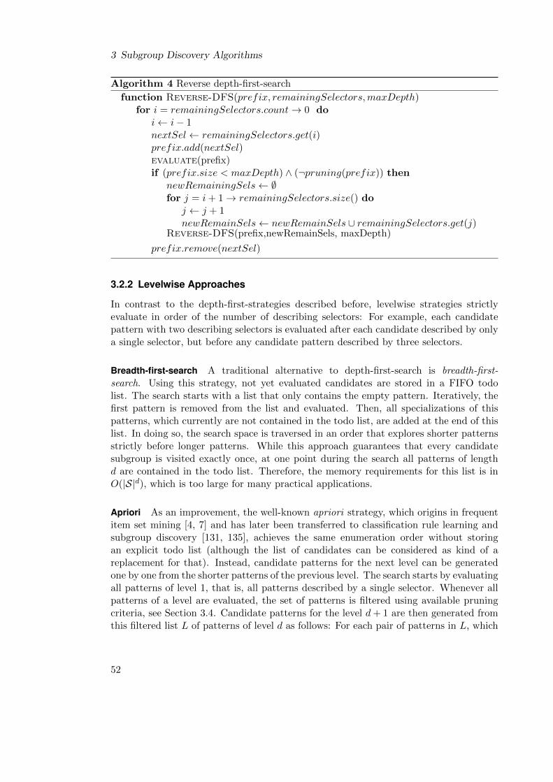
3 Subgroup Discovery Algorithms
Algorithm 4 Reverse depth-first-search
function Reverse-DFS(prefix, remainingSelectors,maxDepth)for i = remainingSelectors.count→ 0 do
i← i− 1nextSel← remainingSelectors.get(i)prefix.add(nextSel)evaluate(prefix)if (prefix.size < maxDepth) ∧ (¬pruning(prefix)) then
newRemainingSels← ∅for j = i+ 1→ remainingSelectors.size() do
j ← j + 1newRemainSels← newRemainSels ∪ remainingSelectors.get(j)
Reverse-DFS(prefix,newRemainSels, maxDepth)
prefix.remove(nextSel)
3.2.2 Levelwise Approaches
In contrast to the depth-first-strategies described before, levelwise strategies strictlyevaluate in order of the number of describing selectors: For example, each candidatepattern with two describing selectors is evaluated after each candidate described by onlya single selector, but before any candidate pattern described by three selectors.
Breadth-first-search A traditional alternative to depth-first-search is breadth-first-search. Using this strategy, not yet evaluated candidates are stored in a FIFO todolist. The search starts with a list that only contains the empty pattern. Iteratively, thefirst pattern is removed from the list and evaluated. Then, all specializations of thispatterns, which currently are not contained in the todo list, are added at the end of thislist. In doing so, the search space is traversed in an order that explores shorter patternsstrictly before longer patterns. While this approach guarantees that every candidatesubgroup is visited exactly once, at one point during the search all patterns of lengthd are contained in the todo list. Therefore, the memory requirements for this list is inO(|S|d), which is too large for many practical applications.
Apriori As an improvement, the well-known apriori strategy, which origins in frequentitem set mining [4, 7] and has later been transferred to classification rule learning andsubgroup discovery [131, 135], achieves the same enumeration order without storingan explicit todo list (although the list of candidates can be considered as kind of areplacement for that). Instead, candidate patterns for the next level can be generatedone by one from the shorter patterns of the previous level. The search starts by evaluatingall patterns of level 1, that is, all patterns described by a single selector. Whenever allpatterns of a level are evaluated, the set of patterns is filtered using available pruningcriteria, see Section 3.4. Candidate patterns for the level d+ 1 are then generated fromthis filtered list L of patterns of level d as follows: For each pair of patterns in L, which
52

3.2 Enumeration Strategies
share the first d− 1 describing selectors, a new candidate with d+ 1 selectors is createdby joining the selector sets of both patterns. For the novel pattern, it is then checkedif also all other generalizations are contained in the list L. Only if this is the case, thenew pattern of level d+1 needs to be evaluated. The search continues by evaluating andgenerating candidates for the next level iteratively until the maximum search depth isreached or no more candidates are generated. Note, that this approach does not requireto store candidate patterns for the last level of search in a list since the patterns canbe generated and evaluated ad hoc from the patterns of the previous level. Therefore,the worst case memory requirements are in O(|S|d−1), by a factor of d smaller than inthe naive breadth-first-search. However, optimized pruning of candidate patterns oftenresults in memory usage that is by orders of magnitudes lower.
The main advantage of apriori in comparison to the depth-first-search approach is thatit provides substantially better pruning options: For each pattern all generalizations arechecked for pruning possibilities before the evaluation of the pattern, while depth-first-search only checks one direct generalization. This is accomplished, however, at the costof increased memory requirements (O(|S|d−1) vs. O(d)).
Algorithm 5 Apriori for subgroup discovery. The evaluations in the for-loop can beaccomplished in a single run over the database, updating the counts for each candidate inparallel. Furthermore, the candidate sets Ck and C ′k are not necessarily built explicitly,especially on the last level of search. Instead, it is sufficient to be able to iterate overthis set. Note, that the algorithm provided here is not identical with the Apriori-SDpresented in [135] since it does omit the wrapper for weighted covering.
function SD-Apriori(maxDepth)L1 ← allSelectorsk ← 2while (Lk−1 6= ∅) do
Lk ← ∅Ck = {X ∪ Y |X,Y ∈ Lk−1, |X ∩ Y | = k − 2} // “generate step”C ′k = {X ∈ Ck|Lk−1 contains k specializations of X} //“prune step”for all c in C ′k do
evaluate(c)if (¬pruning(c)) ∧ (k < maxDepth) then
Lk ← Lk ∪ ck ← k + 1
3.2.3 Best-first-search
Another popular search strategy that is used for the exploration of graphs is best-first-search, see for example [205]. A well known example in this category of search strategiesis the A∗ algorithm for pathfinding. In the best-first approach, all candidates thathave been evaluated by the algorithm, but have not yet been expanded are stored ina todo list, which is sorted by a quality criterion. For supervised pattern mining, an
53

3 Subgroup Discovery Algorithms
upper bound of the interestingness of all respective specializations is used as a sortingcriterion [248, 274]. In each step of the algorithm the first element in the list, that is,the most promising node, is evaluated and expanded by adding its specializations tothe todo list using an optimal refinement operator. The insertion in the todo list canbe skipped if the upper bound for the pattern is lower than the interestingness valuethat is currently required by the result set. Additionally, whenever the quality thresholdin the result set is raised, all candidates with an optimistic estimate below the qualitythreshold can be removed from the todo list. That can be efficiently accomplished sincethe list is ordered by that criterion. Optimistic estimates can be exploited very efficientlyby using best-first-search: Each candidate is evaluated after all other patterns with ahigher optimistic estimate. This increases the likelihood that the pattern is not requiredto be evaluated, because it is pruned beforehand. In a worst case scenario, all subgroupdescriptions of the last level of search are contained in the todo list at some point duringthe search. Therefore, the memory usage can be in O(|S|d). As for Apriori, however,the memory requirements in practical applications is heavily influenced by the qualityof the applied pruning criteria.
As Apriori, this search strategy also guarantees that all generalizations of a patternare always explored before the pattern itself if the upper bound for the interestingnessof a generalization is higher than that of its specialization, which is the case in thetraditional subgroup discovery setting.
Algorithm 6 Subgroup discovery by best-first-search, see also [274]
function best-first-SD(prefix, remainingSelectors,maxDepth)TODO ← {∅} // todo list is initialized with the empty patternwhile not TODO.isEmpty() do
p = TODO.popBest()if (prefix.size < maxDepth) then
Candidates = p.specializations //using an optimum refinement operatorfor all c in Candidates do
evaluate(c)if (¬pruning(c)) then
TODO ← TODO ∪ cpruneAccordingToNewThreshold(TODO)
3.2.4 Beam-search
In contrast to these exhaustive methods, also heuristic methods are often employed forsubgroup discovery. For these methods, the enumeration order does not guarantee totraverse all patterns in the search space. Instead, it tries to find as good patterns aspossible in shorter time by evaluating only promising candidates.
The most popular approach to heuristic supervised pattern mining is beam-search,see e.g. [63]. It follows the intuition that patterns are more likely to have interestingstatistics if also their generalization are interesting. The specification of the algorithm
54
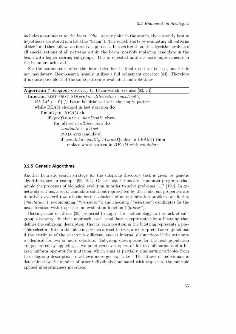
3.2 Enumeration Strategies
includes a parameter w, the beam width. At any point in the search, the currently best whypotheses are stored in a list (the “beam”). The search starts by evaluating all patternsof size 1 and then follows an iterative approach. In each iteration, the algorithm evaluatesall specializations of all patterns within the beam, possibly replacing candidate in thebeam with higher scoring subgroups. This is repeated until no more improvements inthe beam are achieved.
For the parameter w often the desired size for the final result set is used, but this isnot mandatory. Beam-search usually utilizes a full refinement operator [63]. Thereforeit is quite possible that the same pattern is evaluated multiple times.
Algorithm 7 Subgroup discovery by beam-search, see also [63, 14].
function best-first-SD(prefix, allSelectors,maxDepth)BEAM ← {∅} // Beam is initialized with the empty patternwhile BEAM changed in last iteration do
for all p in BEAM doif (prefix.size < maxDepth) then
for all sel in allSelectors docandidate← p ∪ selevaluate(candidate)if (candidate.quality >(worstQuality in BEAM)) then
replace worst pattern in BEAM with candidate
3.2.5 Genetic Algorithms
Another heuristic search strategy for the subgroup discovery task is given by geneticalgorithms, see for example [99, 194]. Genetic algorithms are “computer programs thatmimic the processes of biological evolution in order to solve problems [...]” [194]. In ge-netic algorithms, a set of candidate solutions represented by their inherent properties areiteratively evolved towards the better solutions of an optimization problem by altering(“mutation”), re-combining (“crossover”), and choosing (“selection”) candidates for thenext iteration with respect to an evaluation function (“fitness”).
Berlanga and del Jesus [39] proposed to apply this methodology to the task of sub-group discovery. In their approach, each candidate is represented by a bitstring thatdefines the subgroup description, that is, each position in the bitstring represents a pos-sible selector. Bits in the bitstring, which are set to true, are interpreted as conjunctionsif the attribute of the selector is different, and as internal disjunctions if the attributeis identical for two or more selectors. Subgroup descriptions for the next populationare generated by applying a two-point crossover operator for recombination and a bi-ased uniform operator for mutation, which aims at partially eliminating variables fromthe subgroup description to achieve more general rules. The fitness of individuals isdetermined by the number of other individuals dominated with respect to the multipleapplied interestingness measures.
55

3 Subgroup Discovery Algorithms
3.3 Data Structures
The next section describes different methods how the data can be stored in order toallow for efficient evaluation candidate of subgroup patterns.
3.3.1 Basic Data Storage
The most basic setup uses data directly from a file-system or a database, which is possiblyonly accessible via network. Since access times for these storage devices are by ordersof magnitude slower than for in-memory operations, it is always to be preferred to loadthe complete data in the main memory if possible, i.e., if the available main memory islarge enough for the dataset.
After pre-processing the dataset is stored in a simple tabular form, in our setting asingle table in horizontal layout. That is, similar to relational databases each instanceis stored in one line and each attribute is stored in one column of a table. Cell valuesrepresent the value of the instance of this line for the attribute in the respective column.Whenever a candidate patterns is evaluated, all conditioning selectors are required to bechecked against the original data. Depending on the exact storage system and the com-plexity of the applied selection expressions those checks are potentially time-consuming.Therefore, more advanced approaches apply these checks only once and cache the resultsin optimized data structures, which can then be used for a more efficient mining process.These will be discussed next.
3.3.2 Vertical Data Structures
In a typical application, the data is stored in a so-called horizontal layout. That is,for each case/transaction as key the respective attribute values are stored. For efficientevaluation of subgroup patterns, vertical data representations can be used instead. Thesehave been studied in depth in the field of frequent item set mining [266] and have laterbeen transferred to supervised settings. In these representations, all cases for a patternare stored in a specialized structure, i.e., the subgroup description is used as a key. Thiscan be seen as a 90◦ shift from the typical horizontal data representation, see Figure 3.3
TID-lists TID-lists [266] are basic vertical data representations. In these, each case/-transaction is referenced by a unique (integer) identifier. For each selector in the searchspace as well as for the binary target concept, an ordered list is created from the origi-nal data representation. These contain identifiers of all cases, which are covered by therespective selector, see Figure 3.3 (b) for an example. The mining of the conjunctivesearch space can be accomplished by using only these lists: To compute a TID-list,which corresponds to a conjunction of selectors, one has to determine the list entriesthat are shared by all lists for the single selectors. Since the lists are ordered, this canbe achieved in a single pass over all lists. Of course, TID-lists for conjunctive patternscan be cached and reused to speed up the computation of further specializations. Fortraditional subgroup discovery, the overall instance count and the number of positive
56

3.3 Data Structures
instances are required to compute the interestingness of a pattern. The instance countof a pattern is given by the number of identifiers stored in the TID-list. To obtain thecount of positive instances, the shared members of the respective TID-list and the listfor the target concept are counted.
The memory as well as the runtime requirements are strongly dependent on the size ofthe TID-lists. Therefore, TID-lists are efficient for sparse datasets, where each selectorcovers only a few instances in the database, but are less favorable for dense datasets.
As an improvement for TID-lists, Zaki and Gouda proposed DiffSets [267]. In this datastructure, lists for a conjunction of d selectors are not materialized explicitly. Instead,only the differences to a direct generalization are stored, which can reduce the requiredmemory.
Bitsets An alternative vertical data structure is given by bitsets (also called bitmaps,bitstrings or bitvectors), which have been used for example in the Explora system [139,140]. In these data representations, the instances that correspond to a subgroup patternare stored in words of single bits. Each word contains as many bits as the datasetcontains cases. The i-th bit in each word belongs to the i-th instance in the dataset.The bit is set to 1 if this instance is covered by the respective subgroup description, andis set to 0 otherwise. Similarly to TID-lists, one such bitset is generated for each basicselector and one additional bitset reflects the occurrence of the target concept. Theseinitial bitsets for the selectors can be generated in a single pass over the dataset.
To create bitsets, which correspond to conjunctive patterns, a logical AND operationis performed on the bitsets of the contained selectors. For example, to compute thebitsets which corresponds to the pattern A ∧ B, a bitwise AND is executed on thebitset corresponding to A and the bitset corresponding to B, see Figure 3.3 (c) for anexample. This is especially efficient since most third-generation programming languagesachieve high performances for logical operations on bitsets. The size of a subgroup canthen be derived by determining the cardinality of the bitset, that is, the number of bitsset to 1. The number of positive instances can be computed similarly: A logical ANDis performed on the bitset of the subgroup and the bitset corresponding to the targetconcept. The number of bits with value 1 are counted. For the efficient counting of bitsin a bitset, which are set to true, specialized algorithms and even supporting hardwareimplementations have been developed, see for example [76].
In contrast to TID-lists, the memory requirements for the bitset representation ofa single pattern is independent of the dataset density: For each selector and for thetarget concept a bitsets of length i∅ is required, where i∅ is the number of instances inthe dataset. Thus, the overall memory requirements for the data representation usingbitsets are i∅ ·(|S|+1). Additionally, the runtime for performing a single AND operationbetween data structures does not depend on the data sparseness, unlike to the TID-listapproach.
Sorted representations For the use of vertical data representations in the context ofsubgroup discovery, we have proposed a minor improvement in [177]: Instead of storing
57

3 Subgroup Discovery Algorithms
all instances for a subgroup pattern in a single bitset and then extracting the positiveinstances with an additional AND-operation, one can initially sort the instances withrespect to the target concept into positives and negatives. Then, for each selector twobitsets are created separately, one for the positives and one for the negatives. Rep-resentations for conjunctive patterns are then generated analogously by performing alogical AND on both representations, e.g., bitsets. This approach requires not only oneless AND operation in the evaluation of each subgroup, but can further speedup thecomputation: In a first step the data structure is generated for the positive instancesonly. Then, pruning options can be checked based on this information, for example byexploiting a constraint on the number of positive instances, or by computing optimisticestimates. Thus, the computation of negative instances can potentially be skipped com-pletely. This is especially advantageous in unbalanced data, i.e., if only a small part ofthe data has a positive target concept.
3.3.3 FP-tree Structures and Derivates
FP-trees have been introduced into frequent itemset mining for the well-known FP-Growth algorithm [111] and have later been transferred to the field of subgroup discoverywith binary target concepts [22]. As a major contribution of this work, it will be shownlater in this work how these data structures can be extended for subgroup discoverywith numeric properties of interest and to exceptional model mining, see Chapter 4and Chapter 5.
Mining with FP-trees employs a divide-and-conquer strategy using extended prefixtree structures. Like vertical data structures they provide a condensed but with respectto the task complete representation of the dataset. However, the instances, which arecovered by a pattern, are not directly stored. Instead, aggregated information on thestatistics that are necessary for the evaluation of patterns is saved. For association rulemining, this is the number of instances covered by a pattern, for classical subgroup dis-covery the count of positive and negative instances covered by the pattern. Informationcan be aggregated and conditioned on certain selectors to derive statistics for conjunctivepatterns as necessary.
This section first outlines FP-trees in its original frequent item set mining setting,then adaptations for subgroup discovery are discussed.
Structure and construction of FP-trees A FP-tree consists of tree nodes, which are con-nected by two different types of links. Each tree node (except the root node) correspondsto a selector and stores (in the traditional frequent item set mining setting) a frequencycount. Directed edges between the tree nodes induce a parent-child structure. Pathsfrom the root node to any other node can be interpreted as a conjunction of corre-sponding selectors. Additionally, links between nodes that refer to the same selectorare maintained in a second, auxiliary link structure. A header table aggregates for eachselector the information contained in the respective list.
The construction of FP-trees consists of two steps: In the first step, all simple patternsin the search space are evaluated, filtered using available pruning mechanisms and sorted
58

3.3 Data Structures
id A B Target
1 t t f2 f f f3 t f f4 f t f5 f t f6 f f t7 t t t8 f f t
(a) Horizontal data representation
Target:
A:
B:
A ∧ B:
6 7 8
1 3 7
1 4 5 7
1 7
(b) TID-lists
Target:
A:
B:
A ∧ B:
0 0 0 0 0 1 1 1
1 0 1 0 0 0 1 0
1 0 0 1 1 0 1 0
1 0 0 0 0 0 1 0
(c) Bitsets
∅t: 3, f: 5
Bt: 1, f: 3
At: 0, f: 1
At: 1, f: 1
. . .
(d) FP-tree
Figure 3.3: An examplary dataset in (a) horizontal layout, (b) represented as TID-list,(c) as bitsets, and (d) in a FP-tree. For TID-list and Bitset representation,the data structure for the conjunction A ∧ B is additionally displayed as acomputation example.
59

3 Subgroup Discovery Algorithms
in descending order according to their frequency counts. This order of the selectorsincreases the chance of shared prefixes between data instances, leading to much morecompact representations compared to a lexical ordering. While this ordering step is notnecessarily required, it is therefore highly recommended in literature, see [112].
In the second step, all instances c ∈ I of the dataset are inserted one by one intothe tree structure as follows [111, 22]: First, all selectors in the search space, whichapply in the instance c, are identified and added to an ordered List L according to thepreviously computed frequency order. Then, the insert (L,N) procedure is called withthe complete list L, and the root node of the tree structure as arguments. This methodchecks if there exists a child node that corresponds to the first selector in L. If such anode exists, then the count stored in this node is incremented. Otherwise, such a node iscreated with an initial size of one. The new created node is inserted in the tree structureas child of the last visited node and is also added to the list of nodes corresponding to therespective selector in the auxiliary link structure. In any case, the selector is removedfrom the list L. Unless L is empty, the insert procedure is then called recursively withthe last modified node N and the now shorter list L. Pseudocode of the insert procedureis shown in Algorithm 8.
After the insertion of instances is completed, the information in the header table isactualized. For that purpose, the counts contained in all nodes in the auxiliary list forthis selector are summed up.
Algorithm 8 Insertion of an instance in a FP-tree
function FPTree insert(L,N)nextSelector ← L.pop()nextNode← N.getChild(nextSelector)if nextNode.isNull() then
nextNode← N.createChild(nextSelector, 1)else
nextNode.count++;
if not L.isEmpty() then FPTree insert (nextNode, L)
Conditioning in the FP-tree The header table of the initial FP-tree contains the instancecounts for all basic selectors (items). To determine the counts of conjunctive descriptions(itemsets), so-called conditional trees are used. A conditional tree conditioned on aselector selC can be derived from a FP-tree as follows: First, all prefix-paths from theroot of the tree to the tree leaves that contain selC are identified using the auxiliarylink structure. For each node of these paths the contained count is limited to the countin the lowest (leaf) node. This set of paths describes a new, conditioned dataset thatcontains only those instances, which are covered by selC and only those selectors, whichoccur before selC in the initial ordering. Using these paths, a new smaller FP-tree isconstructed. Of course, conditioning an already conditioned tree on another selector
60

3.4 Pruning Strategies
selC2 , is equivalent to conditioning on a conjunctive pattern. Thus, the search space canbe explored in a recursive manner.
Due to memory restrictions FP-trees are usually applied in combination with a variantof depth-first-search. Also, reordering of the search space is limited to branch reordering:Since each conditional tree contains only selectors that precede the conditioning selectorsin the initial ordering, full reordering can not be applied.
Selectors, which do not appear with the conditioning selector in any instance, are notcontained in the constructed conditional tree. This substantially decreases the size of thetree and the header table. Since these combinations of selectors, which cover no instancesanyway, are not contained in the FP-tree, they are also not explicitly evaluated by thealgorithm. Thus, FP-trees can be considered to have an inherent pruning mechanismregarding not occurring combinations of selectors.
In addition to the techniques presented here, FP-trees exploits specific properties of thetree structure for speedups. Most notably, single-prefix-path allows evaluating patternsin parallel, if they share their only prefix path in the tree structure. For more detaileddescriptions of FP-trees, we refer to [111] and [112].
Adaptation to subgroup discovery A naive approach of utilizing FP-trees for subgroupdiscovery is to use them to identify frequent patterns, and evaluate these candidatepatterns according to the interestingness measure in an independent second phase of thealgorithm, cf. [27]. However, the FP-tree can also easily be exploited for direct miningin the classical subgroup discovery setting: The number of positives p∅ and negatives n∅in the complete dataset (and thus the target share τ∅) can be computed in the initialpass over the dataset. To evaluate a subgroup pattern with respect to a traditionalinterestingness measure, the number of positive and negative instances are requiredfor the respective subgroup. This can be accomplished in a FP-tree by storing not asingle value for the instance count in each node of the tree and the header table, butthe instance counts of positives and negatives separately. Aggregation of nodes can beperformed analogously, adding these two counts up independently from each other. Formore details on the adaptation of FP-trees to subgroup discovery with binary targets,we refer to [22].
Overall, FP-trees have been established as a very efficient data structure, especiallyfor large or sparse datasets.
3.4 Pruning Strategies
Algorithms for subgroup discovery follow a branch-and-bound [164, 65] philosophy asit was introduced in the context of enumeration strategies. The branch step performsthe division of the overall subgroup discovery task into several subtasks, e.g., finding allinteresting descriptions that include a specific selector. These subtasks can be solved to alarge extent independent from each other. The bounds step improves the performance ofthe algorithm by implementing an early detection that the subtasks will not (or unlikely)contribute to the final result. It is distinguished between safe bounds, which only prune
61

3 Subgroup Discovery Algorithms
∅
ba c d
acab ad bc bd cd
abc abd acd bcd
abcd
1
1
1
1
2 2 2
2 2
2
3 3 3 3
4
(a) Unpruned search space
∅
ba c d
ac ad cd
acd
1
1
1
1
2 2 2
3
(b) Pruning at node b
Figure 3.4: The search space of a levelwise search without pruning on the left-hand sideand with pruning at the single pattern b on the right-hand side.
parts of the search space that are guaranteed to not influence the final results, andheuristic bounds, for which this is only unlikely. Thus, exploiting safe bounds neverchanges the overall result, in contrast to heuristic bounds.
As an example for the importance of such pruning possibilities, consider Figure 3.4:Here, the full search tree for a small pattern mining problem is depicted on the left-handside. Now assume that in a levelwise approach the pattern b was evaluated and it couldbe shown that none of its specializations are interesting. As shown on the right-handside of the figure, this cuts the number of patterns to be evaluated on the remaininglevels in half.
As it has been described in literature, implementing advanced pruning bounds canreduce the number of patterns to be evaluated and thus improve the runtime of al-gorithms by orders of magnitude. This can already be achieved by utilizing only safebounds, which will be the focus of this work.
3.4.1 Anti-monotone Constraints
If the subgroup discovery task employs anti-monotone constraints, these can be easilyexploited for pruning the search space. A constraint C(P ) is called anti-monotone if andonly if for each pattern P it holds that
(C(P ) = false) ∧ (S ⊃ P )⇒ C(S) = false,
that is, if a constraint is not satisfied in a pattern P , then it is also not fulfilled inany of its specializations S. Since search strategies generate new candidates from one(as in depth-first-search) or more (as in apriori) generalizations, these anti-monotone
62

3.4 Pruning Strategies
constraints can be easily exploited by not generating candidates for patterns, whichdissatisfy an anti-monotone constraint. Popular anti-monotone constraints include:
� Maximum number of selectors in a subgroup description: By definition each spe-cialization has more selectors than its generalizations, thus the constraint is anti-monotone.
� Minimum subgroup size: Since with each additional describing selector the size ofthe covered instances decreases, this is anti-monotone.
� Minimum number of positives: This is analogous to the constraint before, butlimited to the positive instances.
In contrast to anti-monotone constraints, monotone constraints, e.g., a maximum num-ber of negative examples, are usually not exploited in subgroup discovery algorithms.This is due to the applied general-to-special enumeration order and due to lower perfor-mance gains, since in a depth-limited search most patterns do have significantly morespecializations than generalizations.
3.4.2 Optimistic Estimate Pruning
For subgroup discovery tasks, which are not based on constraints, but on interestingnessmeasures, other pruning options are available: Unfortunately, most measures are notanti-monotone, i.e., strictly decreasing for specializations, themselves. However, formany measures optimistic estimate bounds can be derived and exploited instead. Givena subgroup description P and an interestingness measure q an optimistic estimate oeq(P )is a function such that for each specialization S ⊃ P the interestingness score is notgreater than the value of the optimistic estimate function for the pattern P :
∀S ⊃ P : q(S) ≤ oeq(P )
If the search task aims at finding only subgroup patterns above a certain interesting-ness threshold (e.g., a significance value), then the specializations of all subgroups withan optimistic estimate below this threshold can be skipped in the search: The optimisticestimate property already guarantees that the interestingness value of specializationswill not be sufficient for the specialization to be included in the result set. Optimisticestimates can also be utilized for search tasks that do not employ a fixed quality thresh-old, but a top-k approach. In this case, the interestingness of the pattern with the k-thbest quality found so far, that is, the subgroup with the worst score in the current resultset, can be used as a dynamic minimum quality threshold. Therefore, it depends onthe already evaluated pattern if a pattern can be pruned by using optimistic estimatebounds. As a consequence, the exact enumeration strategy and reordering of the searchspace can be crucial.
63

3 Subgroup Discovery Algorithms
3.4.3 Optimistic Estimates for Common Binary Interestingness Measures
In contrast to the search strategy or the data structure, optimistic estimates dependstrongly on the applied interestingness measure. Therefore, optimistic estimates boundsmust in general be derived for each measure individually.
A simple method to compute these upper bounds is to bound the terms of the interest-ingness measures separately, exploiting the anti-monotonicity of instance counts. Thatis, the number of instances for a specialization is never greater than in its generalization.Consider for example the interestingness measure weighted relative accuracy, which isgiven by q1
bin(P ) = iP · (τP − τ∅). Here, iP is the instance count for the pattern P , τPis the target share in P , and τ∅ is the target share in the overall population. Since theinstance counts of specializations never exceed the instance count of P , and the high-est possible target share is 1, the following optimistic estimate can be derived for thisinterestingness measure, see [260]:
oeq1bin
(P ) = iP · (1− τ∅) = iP · (1− τ∅)
This estimate can be significantly improved using another generic approach: For animportant class of interestingness measures optimistic estimates can be constructed in astraight forward way, that is, for convex measures. An interestingness measure is calledconvex if its value in a fixed dataset is computed by a convex two-dimensional functionq(iP , pP ) over the overall number of instances iP and number of positive instances pPof the evaluated subgroup P . A two-dimensional function f is called convex if and onlyif ∀x1, x2 ∈ R2, λ ∈ [0, 1] : f(λx1 + (1 − λ)x2) ≤ λf(x1) · (1 − λ)f(x2). This can bevisualized such that the function value of each linear combination of two points x1, x2 isalways on or below a straight line between the function values of these parameters. Bythese definitions, some of the most important interestingness measures have been shownto be convex, such as the chi-square measure, the information gain [196], the weightedrelative accuracy and the category utility [274].
For convex interestingness measures q(P ) = q(iP , pP ) it can be shown that an upperbound for the score of any specialization is given by max(q(pP , pP ), q(ip − pP , 0)). Thisdescribes that for any arbitrary pattern the best specialization is given by a refinementthat covers either all positive or all negative instances. Using this approach, an improvedoptimistic estimate for the weighted relative accuracy q1 can be derived [108, 274]:
oeq1(P ) = max(pP · (1− τ∅), (ip − pP ) · (0− τ∅) = pP · (1− τ0)
In an interesting addition to this concept, bounds for (zero-diagonal) convex interest-ingness measures can be further improved, if unavoidable instances are identified, thatis, instances that will be covered by all refinements of a subgroup, cf. [200].
As a minor contribution of this work, the best refinement of a subgroup can also becharacterized for any function, for which the well known axioms postulated in [140],see Section 2.5.3.2, apply:
64

3.5 Algorithms
Theorem 1 Assume that P is a subgroup with a binary target and a target share higherthan the target share in the overall population (τP > τ∅), and q is any interestingnessmeasure for which the well known axioms postulated in [140] (see Section 2.5.3.2) apply.Then, for any subset of the covered instances r ⊆ sg(P ) it holds that:
q(r) ≤ q(s∗), where s∗ = tp(P ) = {c ∈ sg(P )|T (c) = true}
Proof According to the third axiom (“q(P ) monotonically decreases in iP if τp = kiP
with a fixed constant k”) it holds, that q(P ) ≤ q(s∗). Here, the number of positiveinstances pP in P is used as the constant k. This expresses that the interestingness of anysubgroup P with positive quality is always lower or equal compared to the interestingnessof the instance subset, which only contains the positive examples of P .
For arbitrary r ⊆ sg(P ), two cases are now to be considered: If s∗ ⊆ r, then q(r) ≤q(s∗) as shown above, since r contains the same positive instances as s∗, but more (orequal) negative instances. Otherwise it holds that s∗ 6⊆ r, and there exists a subsetr′ = tp(r), which contains only the positive examples of r. Then, as above the thirdaxiom implies that q(r′) ≥ q(r). On the other hand r′ ⊆ s∗ is true, as r′ only coverspositives examples, which are also covered by P . Therefore, the fourth axiom of [140](“q(P ) monotonically increases in iP for a fixed τP > τ∅.”) can be applied: As τr′ =τs∗ = 1 it follows that q(r′) ≤ q(s∗). Thus, it holds that q(r) ≤ q(r′) ≤ q(s∗), provingthe theorem. �
For interestingness measures following these axioms, the highest score for any subsetof the subgroup’s instances is always achieved by the subset that contains exactly allpositive instances. As for convex functions, this can be used to determine an optimisticestimate in a simple way, that is, by computing the interestingness score for this subset.
Despite these results, the computation of optimistic estimates for more complex (non-classic) interestingness measure remains an open issue. In that direction, novel resultsregarding interestingness measures for numeric target concepts and generalization-awareinterestingness measures will be presented in Chapter 4 and Chapter 6.
3.5 Algorithms
The following section provides an overview on algorithms, which have been proposed forsupervised pattern mining in literature. This includes algorithms for descriptive tasks(such as subgroup discovery) as well as predictive tasks (such as rule learning algorithmsfor classification), since the tasks differ very little from an algorithmic point of view, asdiscussed before. The introduced categorization allows for describing the algorithms verysuccinct by referencing the respective enumeration strategy, data structure and pruningstrategy. The used interestingness measures for the method will only be discussed ifpruning strategies, which are specific for certain interestingness measures, are employed.This is, because one easily exchange the measure otherwise.
65

3 Subgroup Discovery Algorithms
Subgroup discovery environments, such as SubgroupMiner [143, 144], Orange1 or Cor-tana2, which incorporate a variety of algorithms, will not be discussed here, since theyonly implement existing algorithms that are described independent of the system. Wedo include, however, the pioneering system Explora due to its historical importancein the field and since the implemented algorithms were innovative at their time. Theoverview here is also limited to algorithm for standard subgroup discovery with a bi-nary target and a traditional interestingness measure. Further algorithms for numerictarget concepts, exceptional model mining and subgroup discovery with generalization-aware interestingness measures are discussed as related work for the novel contributionsin Chapter 4, Chapter 5, and Chapter 6. Additionally, previous algorithm for morespecific scenarios are described separately in Section 3.6.
3.5.1 Explora
The Explora system [140] was one of the first software environments for subgroup dis-covery. It employed a variety of interestingness measures (“evaluation functions”). Sup-ported enumeration orders included exhaustive as well as heuristic approaches, e.g.,(heuristic) best-first-search and depth-first-search. Additionally, filters were utilized tofocus the search on interesting parts of the search space. For the efficient computation ofconjunctions of patterns, Explora did also exploit bitset-based data structures. Exploracould be used to discover patterns with binary or numeric target concepts.
3.5.2 MIDOS
Wrobel [260] proposed the MIDOS algorithm for multi-relational subgroup discovery.The algorithm could be applied using a variety of basic search strategies such as depth-first-search, breadth-first-search or heuristic best-first-search. For performance improve-ments, it employed minimal support pruning as well as optimistic estimate pruning,which exploited an upper bound for the weighted relative accuracy interestingness mea-sure. Specialized data structures are to the author’s knowledge not described for thissystem. However, the system makes use of sample strategies for applicability in largescale domains.
3.5.3 The CN2 Family
CN2 [63, 62] is a classical rule learning algorithm for classification. It utilizes a beam-search method to identify the “best” rule according to a rule heuristic. The selectionof a single rule is embedded in a sequential covering approach [193]. The algorithmCN2-SD [165] extends this approach by adding a weighted covering scheme, see Sec-tion 2.5.5.1. Since the focus of this line of research is more on the expressiveness of therule set than on scalability, there are no especially efficient data structures specified for
1http://orange.biolab.si2http://datamining.liacs.nl/cortana.html
66

3.5 Algorithms
these algorithms. Additionally, no additional pruning criteria for efficient rule identifi-cation have been described. The CN2-SD algorithm has also been extended by variantsfor subgroup discovery with multi-class targets [3] (called CN2-MSD) and relationalsubgroup discovery [169, 270] (called RSD).
3.5.4 OPUS
Webb introduced OPUS as a general algorithm for unordered search that follows abranch-and-bound philosophy [248]. It has also been used for supervised rule learning.OPUS is proposed in two different variations: WhileOPUSS focuses on satisfying search,OPUSO is used for optimization search, that is, to find the best node in the searchspace according to an evaluation function. It describes the use of “optimistic pruning”in combination with a best-first strategy to explore the search space.
No specialized data structure is described. In the context of classification rule learn-ing, Webb also introduced optimistic estimates for specific “preference functions” forOPUS, i.e., the maximum consistent preference function and the Laplace preferencefunction [256]. The algorithm is currently the center-piece of the commercial MAGNUMOPUS software for association discovery. In the original publication, a depth-first-searchwith reordering according to the optimistic bound is recognized as an alternative enu-meration order for settings, in which memory is critical.
3.5.5 SD
The algorithm SD [92] also uses a beam-search strategy for enumeration. Regardingpruning, it utilizes simple support pruning. Additionally, irrelevant subgroups are neveradded to the beam. No specialized data structures are specified. The description ofthe algorithm emphasizes the interactive nature of the addressed task. Therefore, thealgorithm is embedded in an environment featuring different interestingness measuresand visualizations.
3.5.6 STUCCO
For mining contrast sets, Bay and Pazzani proposed the STUCCO algorithm [32, 33],which searches for interesting patterns in a breadth-first strategy. For pruning, supportthresholds for different groups are used as well as an optimistic estimate bound for theχ2 measure. Additionally, specializations that have the same support as generalizationsare pruned, as they are considered as not interesting.
3.5.7 Apriori-C and Apriori-SD
Jovanovski and Lavrac adapted the Apriori algorithm for itemset mining to obtain clas-sification rules [131]. In addition to standard support pruning, also another pruningcriterion is used. It filters specializations, for which a generalization already is consid-ered as interesting based on support and confidence thresholds. However, neither strictoptimistic estimates nor specialized data structures are described. The classification
67

3 Subgroup Discovery Algorithms
centered algorithm Apriori-C has later been transferred to subgroup discovery in an al-gorithm called Apriori-SD [167]. The changes mainly focus on a different interestingnessmeasure and the introduction of a new covering scheme, i.e., weighted covering, to avoidredundancy.
3.5.8 Apriori SMP
Morishita and Sese [196] introduced the AprioriSMP algorithm for association rule min-ing with a fixed conclusion. They combine the levelwise apriori enumeration order with“statistical metric pruning”, which is equivalent to optimistic estimates in the terminol-ogy of this work. For their algorithm, they provide upper bounds for the interestingnessmeasures chi-square, entropy gain, gini-index, and the correlation coefficient measuringthe correlation between the description and the target. For AprioriSMP, no specializeddata structure has been proposed.
3.5.9 Harmony
The Harmony algorithm for mining classification rules [246] performs a depth-first-searchwith different reordering options, e.g., reordering depending on confidence, entropy or acorrelation measure. It also supports pruning based on optimistic estimates by combiningthe support threshold with the confidence function, which is used as interestingnessmeasure.
3.5.10 CorClass and CG
The CorClass algorithm [273] was proposed by Zimmermann and de Raedt for the min-ing of class association rules, that is, association rules with the fixed class attributeof the dataset as a consequence. The algorithm emphasizes the usefulness of optimisticestimate pruning. To maximize the benefits of the bounds, they propose a best-first enu-meration strategy and utilize general upper bounds for convex interestingness measures.No specialized data structures are mentioned.
The algorithm was refined into the CG-algorithm [274] with similar computationalproperties regarding pruning- and search strategy. In this approach, the supervisedpattern mining task is not only regarded as a stand-alone task as in subgroup discovery,but also as a core step for other areas such as classification or (conceptual) clustering.
3.5.11 Corrmine
The Corrmine algorithm for correlated itemset mining [200] exploits additional bounds(4-bounds) by propagating itemsets, which are unavoidable, in addition to traditionaloptimistic estimates. This is embedded in an algorithm based on ECLAT [269] thatemploys a depth-first-search and vertical data representations.
68
3.5 Algorithms
3.5.12 SDIGA and MESDIF
Del Jesus et al. propose the genetic algorithm SDIGA for a subgroup discovery taskin the context of a case study in the domain of marketing [68]. They utilize a fuzzydiscretization of numeric variables as well as (internal) disjunctions in rule description,which is claimed to still provide an “explanatory and understandable form that can beused by the expert” [68]. The fitness of individuals is assigned by measuring the numberof individuals in a population, which are dominated by a pattern with respect to thethree applied objectives (interestingness measures), confidence, support and “originalsupport”. Another closely related algorithm presented in the same domain is MES-DIF [39].
3.5.13 Algorithm of Cerf
Cerf et al. propose an algorithm for mining class association rules [57]. Their algorithmemploys a breadth-first enumeration strategy. Regarding pruning, only basic pruningbased on the support of the pattern is used. Additionally, specializations of patterns,which are considered as interesting, are not explored. The search is repeated for eachvalue of the target attribute, carrying over already discovered interesting patterns. Nospecialized data structure is described.
3.5.14 CCCS
The CCCS -algorithm tries to find rules for associative classification in imbalanced dataefficiently [12]. The search is performed in a depth-first manner. Interestingly, thesearch space is build explicitly by adding transactions (instances) one-by-one into anenumeration tree. This resembles a feature of FP-trees, in which also non-occurringpatterns are left out from the start. However, in this approach a pass over the dataset isrequired for each candidate. Additionally, no pruning schemes are exploited to enhancethe performance.
3.5.15 CMAR
For improved classification based on associations, the CMAR algorithm [179] was in-troduced. For the efficient mining of rules, it employs a variation of FP-trees as datastructure in a depth-first-search. No optimistic estimate pruning is described.
3.5.16 SD-Map
The SD-Map algorithm [22] transferred the FP-tree data structure to the subgroup dis-covery setting. The algorithm employs a strict depth-first-search enumeration strategy.For pruning, only constraints for the subgroup size and the number of positive instancesare utilized, but no optimistic estimate pruning.
69
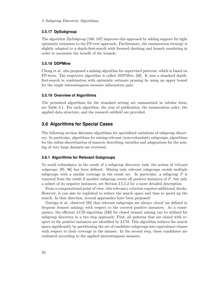
3 Subgroup Discovery Algorithms
3.5.17 DpSubgroup
The algorithm DpSubgroup [100, 107] improves this approach by adding support for tightoptimistic estimates to the FP-tree approach. Furthermore, the enumeration strategy isslightly adapted to a depth-first-search with forward checking and branch reordering inorder to maximize the benefit of the bounds.
3.5.18 DDPMine
Cheng et al. also proposed a mining algorithm for supervised patterns, which is based onFP-trees. The respective algorithm is called DDPMine [60]. It uses a standard depth-first-search in combination with optimistic estimate pruning by using an upper boundfor the single interestingness measure information gain.
3.5.19 Overview of Algorithms
The presented algorithms for the standard setting are summarized in tabular form,see Table 3.1. For each algorithm, the year of publication, the enumeration order, theapplied data structure, and the research subfield are provided.
3.6 Algorithms for Special Cases
The following section discusses algorithms for specialized variations of subgroup discov-ery. In particular, algorithms for mining relevant (non-redundant) subgroups, algorithmsfor the online-discretization of numeric describing variables and adaptations for the min-ing of very large datasets are reviewed.
3.6.1 Algorithms for Relevant Subgroups
To avoid redundancy in the result of a subgroup discovery task, the notion of relevantsubgroups [95, 96] has been defined. Mining only relevant subgroups avoids multiplesubgroups with a similar coverage in the result set. In particular, a subgroup P isremoved from the result if another subgroup covers all positive instances of P , but onlya subset of its negative instances, see Section 2.5.5.2 for a more detailed description.
From a computational point of view, this relevancy criterion requires additional checks.However, it can also be exploited to reduce the search space and thus to speed up thesearch. In that direction, several approaches have been proposed:
Garriga et al. observed [95] that relevant subgroups are always closed (as defined infrequent itemset mining) with respect to the covered positive instances. As a conse-quence, the efficient LCM -algorithm [240] for closed itemset mining can be utilized forsubgroup discovery in a two step approach: First, all patterns that are closed with re-spect to the positive instances are identified by LCM. This algorithm reduces the searchspace significantly by partitioning the set of candidate subgroups into equivalence classeswith respect to their coverage in the dataset. In the second step, these candidates areevaluated according to the applied interestingness measure.
70

3.6 Algorithms for Special Cases
Tab
le3.
1:A
nov
ervie
wof
sup
ervis
edp
atte
rnm
inin
gal
gori
thm
s,ca
tego
rize
dw
ith
resp
ect
toen
um
erat
ion
stra
tegy
,p
run
ing
stra
tegy
,d
ata
stru
ctu
re,
and
orig
inal
rese
arch
fiel
d.
Alg
orit
hm
Yea
rE
nu
m.
stra
tegy
Pru
nin
gD
ata
stru
ctu
reR
esea
rch
fiel
d
Ap
rior
i-C
2001
leve
lwis
esu
pp
ort+
spec
ial
-cl
assi
fica
tion
rule
s
Ap
rior
i-S
D20
04le
velw
ise
sup
por
t+sp
ecia
l-
sub
grou
pd
isco
very
Ap
rior
i-S
MP
2000
level
wis
eop
t.es
t.-
ass.
rule
sw
/fi
xed
con
cl.
CC
CS
2006
DF
S-
-as
soci
ativ
ecl
assi
fica
tion
Cer
f20
08b
read
th-fi
rst
sup
por
t-
asso
ciat
ive
clas
sifi
cati
on
CM
AR
2001
DF
S-
FP
-tre
esas
soci
ativ
ecl
assi
fica
tion
CN
219
89B
eam
--
clas
sifi
cati
onru
les
CN
2-S
D20
02B
eam
--
sub
grou
pd
isco
very
Cor
rCla
ss20
09B
est-
firs
t-op
top
t.es
t.-
seve
ral
Cor
rmin
e20
09D
epth
-firs
top
t.es
t.+
4-b
oun
ds
dep
th-fi
rst
corr
elat
edit
emse
tm
in.
DD
PM
ine
2008
DF
Sop
t.es
t.F
P-t
rees
dis
crim
inat
ive
pat
tern
s
Dp
Su
bgr
oup
2008
DF
S+
FC
opt.
est.
FP
-tre
essu
bgr
oup
dis
cove
ry
Exp
lora
1996
DF
S,B
FS
,Bes
t-F
irst
red
un
dan
cyb
itse
tssu
bgr
oup
dis
cove
ry
HA
RM
ON
Y20
05D
FS
+R
eord
erop
t.es
t.-
clas
sifi
cati
onru
les
MID
OS
1997
DF
S,B
est-
Fir
stop
t.E
st-
mu
lti-
rela
tion
al
OP
US
1995
Bes
t-F
irst
-Op
top
t.es
t.-
gen
eral
sear
ch
SD
2003
Bea
msu
pp
ort+
rele
van
ce-
sub
grou
pd
isco
ver
y
SD
IGA
2007
Gen
etic
--
sub
grou
pd
isco
very
SD
-Map
2006
DF
Ssu
pp
ort
FP
-tre
essu
bgr
oup
dis
cove
ry
ST
UC
CO
1999
BF
S,(
DF
S)
sup
por
t-
contr
ast
set
min
ing
71

3 Subgroup Discovery Algorithms
An extension of this approach by Boley and Grosskreutz focuses on the identificationof minimum representatives for each equivalence class [42]. The resulting algorithm imris reported to match the performance of the standard algorithm DpSubgroup (cf. Sec-tion 3.5.17) in datasets, in which the compression through equivalence classes is high.
In previous work, the author of this work performed a comparison of data structuresfor the mining of irrelevant subgroups [171, 177]. It turned out that vertical data struc-tures are better suited for this task than FP-tree-based structures, since they allow forperforming efficient relevance checks directly in the search algorithm. The proposedalgorithm BSD combines depth-first-search, a bitset-based data representation, and op-timistic estimate pruning with (optional) efficient relevancy checks. However, the algo-rithm can not theoretically guarantee to obtain the best relevant subgroups, althoughthey are almost always found in practice. This problem is caused by the fact that promis-ing subgroups, which are first added to the top-k result set, are shown to be irrelevantlater in the search process and thus have to be removed from the result. Grosskreutzand Paurat solved this problem by employing an iterative deepening depth-first-searchas enumeration strategy [104].
Recently, Grosskreutz introduced another algorithm, which is able to enumerate allrelevant subgroups in polynomial time with respect to the result size [101]. It utilizesa more precise characterization of candidate subgroup than the closed-on-the positivesproperty. This is exploited by a new relevance check based on the direct generalizationsof a subgroup in order to apply more effective pruning in the search algorithm. Thealgorithm uses breadth-first-search as enumeration strategy.
3.6.2 Numeric Selectors
As discussed in Section 2.3.2, numeric attributes in the search space can be incorporatedin standard mining algorithms through discretization in a pre-processing step. Since thisinvolves loss of information, online-discretization, i.e., identifying the best intervals fornumeric attributes within the subgroup mining algorithm, has been postulated. However,this can increase the search space of subgroup discovery substantially. In order to handlethis problem efficiently, specialized subgroup discovery algorithms have been proposedfor this setting:
The MergeSD algorithm [106] of Grosskreutz and Rueping is designed for exhaustivesearch. It exploits that for the Kloesgen measures qaKl(P ) = iP
a · (τP − τ∅) an optimisticestimate for a subgroup description P ∧A ∈ ]tl, tr[ can be calculated based on statisticalinformation regarding the patterns P ∧ A ∈ ]tl, t
′[ and P ∧ A ∈ ]t′, tr[ for any numericattribute A and tl ≤ t′ ≤ tr. Information on the derived bounds is stored in a specializeddata structure called boundTable. The pruning scheme is integrated in a depth-first-search with look-ahead.
Mampaey et al. analyzed the refinement step for greedy algorithms such as beam-search (cf. Section 3.2.4) with respect to online discretization of numeric describingattributes [189]. They propose a method that allows for finding the best interval ofa numeric attribute that is added to the current subgroup description in linear timeof the number potential cutpoints, in contrast to the quadratic time required by the
72

3.6 Algorithms for Special Cases
trivial approach. This is accomplished by focusing on the subgroups, which are on theconvex hull of candidate subgroups in the ROC space. These can be determined effi-ciently bottom-up from the convex hulls of the basic half-open intervals using Minkowskidifferences.
In the field of association rule mining, related approaches have been discussed: Fukudaet al. investigated numeric attributes in the rule condition of optimized associationrules [84]. These aim at identifying intervals for numeric attributes, which imply amaximum confidence for the rule. For efficient mining, the authors exploit convex hulltrees in order to compute the best interval for one attribute with respect to the ruleconfidence in linear time. This problem setting has been extended in [214, 46] to includedisjunctions of intervals.
3.6.3 Large Scale Mining Adaptations
Although sophisticated mining algorithms improve the scalability of subgroup discoveryby orders of magnitude, the proposed methods may still be intractable for very largedatasets. Besides optimizing existing algorithms and decreasing the complexity of thesearch, e.g., by selecting a subset of relevant attributes or by setting a limit for the max-imum number of selectors in a subgroup description, there are two different possibilitiesto handle specifically very large datasets: sampling and parallelization.
3.6.3.1 Sampling
Sampling describes the (random) selection of a subset of the current dataset. Charac-teristics of the complete dataset can be estimated from the characteristics of the sample.These can be determined more efficiently due to the smaller size of the sample.
A first line of research focuses on deriving guarantees about the quality of resultsderived from a specific, randomly drawn sample. This can be modified to determinethe size of the sample set, which is required to guarantee that the computed quality fora pattern exceeds a given threshold. In that direction, Schaeffer and Wrobel proposedthe GSS algorithm (Generic Sequential Sampling) [218, 220]. It iteratively draws newinstances from the database, until it can be guaranteed with a certain confidence thatthe current k best hypotheses are the overall best hypotheses in the dataset. Thistechnique was explored for a variety of interestingness measures. The original algorithmrequires all hypotheses (subgroups) to be stored in memory. An improved version of thealgorithm, LCM-GSS, only requires fixed memory, but this comes at the cost of largersample sizes [219].
These algorithms aim at achieving samples of the dataset, which approximate thedistributional properties of the overall dataset as close as possible. Other approaches aimat the selection of representative instances instead of random subsets. In that direction,several strategies have been proposed in the related field of association rule mining, e.g.,the FAST algorithm [58] or the ε-approximation algorithm [49]. Regarding subgroupdiscovery, Cano et al. investigated different sample strategies, e.g., by employing anearest neighbor prediction approach [56].
73

3 Subgroup Discovery Algorithms
A few other approaches use the sampling procedure to alter the distributions in orderto obtain subsets of instances, which are particularly interesting or useful. In that di-rection, Scholz presents a method to incorporate background knowledge into subgroupdiscovery [222, 221]. It utilizes directed sampling to prevent the rediscovery of priorknowledge. This is done by re-weighting instance for the sampling according to previ-ously known patterns. In another study by Cano et al., a stratified selection algorithmis explored, which increases the presence of the minority class in imbalanced data, thatis, a dataset, in which one value of the target concept occurs much more frequently thanthe other [55].
Traditional sampling methods select subsets of instances in the dataset. Recently,some novel approaches have been proposed that focus on sampling subsets of patternsinstead. In that direction, Boley and Grosskreutz proposed a method, which uses aMarkov chain Monte Carlo method (MCMC) to sample local patterns such as associationrules or subgroups [41]. To overcome the scalability issues of MCMC an alternative two-step approach has been proposed [43]: In a first step a few data instances are drawn,then local patterns are sampled based on the drawn instances.
3.6.3.2 Parallelization
A second possibility to handle very large datasets is to assign subtasks to differentcomputation units, which can operate at the same time. Two kinds of parallelizationtechniques can be distinguished, see for example [162]: Multicore computing describesthat several processing units of one machine are involved in the computation. In thisscenario, the same data is available for all cores in the shared memory. In contrast,distributed computing describes data processing on different machines, which are onlyconnected by a network and use separate memory stores.
Parallel subgroup mining with shared memory is relatively simple to implement andto adapt by many discovery algorithms. The branches of the search tree can be assignedto different computation units, which explore their respective part of the search treeindependent of each other. The only required communication is concerned with thepropagation of the minimum interestingness score of the result set for optimistic estimatepruning. Additionally, computation units can reassign parts of their assigned task toidle units if these completed their task earlier. This provides for simple load-balancing.This kind of parallelization has been implemented successfully in subgroup discoverysystems, e.g., in the MIDOS system [260] or for the algorithm BSD [177].
Subgroup mining in a distributed scenario is much more complicated: Communicationcosts, e.g., for propagating the requirements for optimistic estimate pruning, have to bestrongly considered in this case. Wurst and Scholz investigated a setting, in which thedata is distributed among several nodes (computation units) [264]. For this setting, theypropose an algorithm, in which each subgroup pattern is assigned to a node. This nodedecides if pruning can be applied for this pattern. If not, then count polling is initiated,that is, the counting of positives and negatives in all nodes. After results are collected, itis determined if specializations of the current rule are potentially interesting. In this case,specializations are generated and assigned for evaluation to other computational nodes in
74
3.7 Summary
the network. Pruned subgroups and changes in the result set are always communicated toall nodes, leading to communication costs that increase linearly with number of evaluatedsubgroups and computation nodes. Another distributed subgroup mining algorithm thatespecially emphasizes the data privacy for each node is proposed by Grosskreutz et al.in [103].
In the related field of association rule discovery, several approaches have been presentedfor distributed mining, see also [217]. Different approaches cover the distribution of thedata to different nodes, the distribution of candidates to different nodes, or a combinationof both [6, 61, 268, 224]. Several methods focus on distributed computations for the FP-tree data structure [51, 123]. Adapting these methods seems to be a promising directionfor future subgroup discovery research.
3.7 Summary
This chapter provided an overview on efficient supervised pattern mining algorithmsfrom literature. This overview included not only algorithms that use the terminologyof subgroups discovery, but also algorithms from closely related fields. It presentedmethods for different algorithmic components in detail, that is, for the enumerationstrategy, for the data representation, and for the pruning strategy. Algorithms couldthen concisely be described in terms of these components. Beside the standard super-vised pattern mining setting, also some important variations have been outlined, suchas the discovery of relevant subgroups and subgroup discovery with numeric describingattributes. Regarding large scale applications, methods for sampling and parallelizationwere summarized.
75


4 Algorithms for Numeric Target Concepts1
Practical applications often involve numeric attributes with a continuous domain asthe target property of interest. Although it is possible to transform this problem set-ting to the standard nominal one by using discretization techniques in a pre-processingstep [78, 157], this yields a possibly crucial loss of information. Therefore, over theyears a variety of interestingness measures has been proposed, which are directly basedon the distribution of a numeric target attribute. These have been summarized in Sec-tion 2.5.3.3.
For example, a potentially interesting subgroup using target discretization could beexpressed as “While in the general population only 6% of the people are older than80, in the subgroup described by xy it is 12%”. In contrast, using the distributionof the numeric targets concept directly with a mean-based interestingness measure, asubgroup is described like “While in the general population the mean age is 56 years,in the subgroup described by xy it is 62”. Until now, the numeric target setting is lessintensively studied than the traditional case with binary targets. Therefore, this chapterinvestigates this scenario in detail and proposes several improvements for the efficientexhaustive mining of subgroups with numeric target settings.
As discussed in Chapter 3, algorithms are characterized by the employed enumerationstrategy, by the used data structure, and by the applied pruning strategy, which allowsto omit parts of the search space safely. Since the search space does not change, if anumeric target concept is used instead of a binary one, enumeration strategies can bedirectly transferred from the traditional setting with binary targets. Instead, this workfocuses on optimistic estimate bounds for efficient pruning of the search space and onthe adaptation of data structures specialized for this problem setting. In more detail,the contributions of this chapter are the following:
1. For a large variety of interestingness measures, novel optimistic estimate boundsare introduced. These are used for pruning the search space: If it can be proventhat no subset of a subgroup’s instances induces a sufficiently high interestingnessscore to be included in the result set of subgroups, then no specialization of thissubgroup is included in the result. These specialization can be skipped in thesearch process without influencing the optimality of the result. We distinguishbetween bounds with closed-form representations and bounds based on ordering,which allow the computation of optimistic estimate by checking few candidatesubsets of instances.
1A minor part of this chapter, i.e., the introduction of the SD-Map* algorithm, has previously beenpublished as [15]: Martin Atzmueller and Florian Lemmerich. Fast Subgroup Discovery for Con-tinuous Target Concepts. In Proceedings of the 18th International Symposium on Foundations ofIntelligent Systems (ISMIS), 2009.
77
4 Algorithms for Numeric Target Concepts
2. It is shown how the most important data representations, i.e., FP-trees and bitsetdata structures can be adapted to the problem setting of numeric target concepts.It is shown that the application of different data structures allows for the applica-tion of different optimistic estimate bounds.
3. Two novel algorithms called SD-Map* and NumBSD implement these approachesand allow for efficient mining in practical applications. Both algorithms applyoptimistic estimate pruning, but utilize different core data structures and thuspossibly different pruning bounds. Both outperform simple approaches by ordersof magnitudes.
4. For the proposed bounds and algorithms an extensive experimental evaluationon publicly available datasets is provided. These show the benefits of the novelapproaches and aim also to identify recommendations for choosing the best miningalgorithm for specific tasks.
The rest of the chapter is structured as follows: It starts by summarizing previous ap-proaches to subgroup discovery with numeric target concepts in Section 4.1. After that,novel optimistic estimate bounds for these measures are introduced in Section 4.2. Then,modifications of data representations for the numeric setting are discussed in Section 4.3.Next, Section 4.4 presents two practical algorithms for efficient subgroup discovery withnumeric targets. Section 4.5 provides an evaluation of the presented approaches. Com-putational properties of the different interestingness measures are summarized in Sec-tion 4.6, before we conclude in Section 4.7.
4.1 Related Work
Generally, subgroup discovery with numeric target concepts can be performed by ap-plying discretization on the target concept. In doing so, the task is transformed into astandard subgroup discovery task with a binary target concept. A discretization method,which was specifically designed for numeric targets in subgroup discovery, is TargetClus-ter [195]. It uses a scoring of clustering solutions to find appropriate intervals for thetarget concept. Nonetheless, discretizing the target concept leads to a loss of informa-tion, see also Section 2.5.3.3.
Subgroup discovery with numeric target concepts without discretization has been in-troduced in the pioneering system Explora [140]. It applied a variety of enumerationstrategies for subgroup discovery. Regarding numeric attributes, it was able to identify“mean patterns”, that is, subgroups with a significantly deviating mean value in the nu-meric target attribute in comparison to the total population. An exemplary case studyfor this system using mean patterns is provided in [138]. For Explora, no optimistic es-timates or data structures, which are specific for the mining of subgroups with numerictarget concepts, are described.
Later, Aumann and Lindell [27, 28] discussed this problem setting in the context ofassociation rules, described as quantitative association rules. For the discovery of desiredrules, they apply a three-stage process: First, all frequent patterns in the search space
78

4.2 Optimistic Estimates
are mined by a standard frequent itemset mining algorithm, i.e., Apriori. In a secondstep, an interestingness value of these patterns is computed based on the deviation ofeither the mean or the variance of the target. Sub-rules, which are contained in moregeneral rules are then filtered out in a third step. As a result of this multi-stage process,pruning is only based on the support of the patterns. In contrast to this method, theapproach described in this work focuses on the direct mining of interesting patternsin one step. This allows for the application of advanced pruning techniques that cansubstantially improve the mining performance.
Webb [249] utilizes a best-first approach to efficiently find association rules with aspecific numeric variable in the rule head. In this approach, optimistic estimate pruningis applied for the utilized interestingness measure. The presented upper bounds arehowever limited to a single interestingness measure (“impact rules”, which is equivalentto q1
mean in the terminology of this paper). In contrast, this chapter presents upperbounds for a wide variety of interestingness measures. In addition, adaptations to datastructures are discussed, which allow for the efficient computation of interestingnessmeasures and their upper bounds.
Jorge et al. present an algorithm for the discovery of distribution rules called CAREN-DR [130]. These can be considered as subgroups for a numeric target concept that use aKolmogorov-Smirnov-based interestingness measure. The algorithm follows a depth-firstenumeration order. It utilizes (unordered) bitsets to speedup the evaluation of patterns.Pruning is limited to support pruning and does not take advantage of optimistic esti-mates.
Pieters et al. discuss different interestingness measures [210, 209] for subgroup discov-ery with numeric targets. However, they focus on the performance of different measuresand do not investigate techniques for efficient exhaustive mining.
4.2 Optimistic Estimates
Optimistic estimates are upper bounds for the interestingness score of all specializationsof a subgroup. They are used to speedup the search process for subgroup discovery: Ifthe optimistic estimate of a subgroup is lower than the interestingness value required inthe result set, then the specializations of this subgroup can be excluded from the search,see also Section 3.4.2. As research for binary target concepts has shown, this can reducethe number of candidate subgroups in discovery algorithms by orders of magnitudes.Nonetheless, for subgroup discovery with numeric target concepts, optimistic estimatebounds have only received limited attention in literature so far.
This section thoroughly analyzes optimistic estimate pruning for subgroup discoverywith numeric target concepts for a large variety of interestingness measures. It showsfirst why the problem of deriving optimistic estimates is more difficult for numeric targetsthan in the traditional binary target setting. Then, optimistic estimates in closed-formexpressions are derived for the discussed interestingness measures. These upper boundscan also be determined by algorithms that use a FP-tree like data structures. Next,a property of interestingness measures is introduced that allows intuitive derivation
79

4 Algorithms for Numeric Target Concepts
Table 4.1: Derivation of the best subset of example subgroup P . The subset with thebest interestingness score for a measure is printed in bold. It can be seen thatthe subset differs for different interestingness measures.
Target values of asubset r ⊆ sg(P )
q1mean(r) q0.5
mean(r) q0mean(r)
{100} 1 · (100− 50) = 50√
1 · (100− 50) = 50 100− 50 = 50
{100, 75} 2 · (87.5− 50) = 75√
2 · (87.5− 50) ≈ 53 87.5− 50 = 37.5
{100, 75, 53} 3 · (76− 50) = 78√
3 · (76− 50) ≈ 45 76− 50 = 26
{100, 75, 53, 12} 4 · (60− 50) = 40√
4 · (60− 50) = 20 60− 50 = 10
of upper bounds. In addition to these bounds, a novel approach provides a series ofincreasingly tight upper bounds, which can be computed by using only a part of theinstances covered by a subgroup.
4.2.1 Differences to the Binary Setting
An optimistic estimate bound of a subgroup is given by the subset of instances, whichimplies the highest score according to the used interestingness measure. In the traditionalsetting with a binary target concept, it is easy to determine this subset, as long as theinterestingness measures follow the common axioms of Piatetsky-Shapiro and Major &Mangano, see 2.5.3.2: The best subset is the set of all instances that have a positive targetconcept, see Theorem 1. In contrast to that, the continuous case is more challenging.Here, the best refinement of a subgroup depends on the applied interestingness measure,as demonstrated in the following example:
Example 1 Assume a dataset with an average target value of µ∅ = 50. We determinethe best refinement for a subgroup P according to mean-based interestingness measuresqamean(P ) = iP
a · (µP − µ∅), with a = 0, a = 0.5, and a = 1. In this example Pcovers 4 instances: sg(P ) = {c1, c2, c3, c4}. The target values for these instances areT (c1) = 100, T (c2) = 75, T (c3) = 53 and T (c4) = 12. Then, for the interestingnessmeasure impact q1
mean the subset with the best interestingness score contains the threecases with values 100, 75, and 53, see Table 4.1. On the other hand, for the mean testinterestingness measure q0.5
mean, it contains two cases with the values 100 and 75. For theaverage interestingness measure q0
mean, the best subset contains only the instance withvalue 100. 2
Since a simple and effective way to derive optimistic estimate bounds is to computeor estimate the interestingness value of the best refinement, the task of deriving upperbounds for all specializations is significantly more challenging for a numeric target con-cept. Another reason is that in the binary case the complete distribution of the targetconcept in a subgroup is precisely specified by just two numbers (the numbers of positiveand negative examples), but it is more complex to describe in the numeric case.
80

4.2 Optimistic Estimates
4.2.2 Optimistic Estimates with Closed Form Expressions
Next, novel optimistic estimates are derived for the interestingness measures that havebeen discussed in Section 2.5.3.3. The estimates presented below have a closed-formexpression that uses a limited amount of statistics derived from the subgroup. In par-ticular, the bounds for a single subgroup are computable in a distributed single-passalgorithm. Thus, these statistics are also computable in efficient FP-tree data struc-tures, as will be shown in Chapter 5, which analyzes applicability issues of this datastructure in general.
4.2.2.1 Mean-based Interestingness Measures
Theorem 2 As described in [249], an optimistic estimate for the impact interestingnessmeasure q1
mean(P ) = iP · (µP − µ∅) is for any subgroup P given by:
oe1mean(P ) =
∑c∈P :T (c)>µ∅
(T (c)− µ∅).
This estimate is tight.
Proof We reformulate this interestingness measure:
q1mean(P ) = iP · (µP − µ∅)
= iP · (∑
c∈sg(P ) T (c)
iP− iP · µ∅
iP)
=∑
c∈sg(P )
T (c)− iP · µ∅
=∑
c∈sg(P )
(T (c)− µ∅)
For all subsets r ⊆ sg(P ), this sum reaches its maximum for the instance set r∗, whichcontains all cases with larger target values than the average of the population. For thisset of instances, the summand in the above formula contains all positive summands,but no negatives ones. The interestingness score for r∗ is given by q1(r∗) = oe1
mean(P )using the above formula. As no other subset of sg(P ) leads to a higher interestingness,oe1mean(P ) is an upper bound for the interestingness score of all specializations of P and
an optimistic estimate. Since for any given subgroup the estimate is reached by one ofits subsets, the estimate is tight. �
Interestingly, the tight optimistic estimate for the binary case presented in [108], i.e.,pP · (1 − τ∅), can be seen as special case of this formula, considering T (c) = 1 for truetarget values and T (c) = 0 for false target values:
oe1mean(P ) =
∑c∈sg(P ),T (c)>µ∅
(T (c)− µ∅) =∑
c∈sg(P ),T (c)=1
(1− τ∅) = pP · (1− τ∅).
81

4 Algorithms for Numeric Target Concepts
This optimistic estimate bound can easily be extended to the other generic mean-basedinterestingness measures qamean:
Theorem 3 oe1mean(P ) is an optimistic estimate for any generic mean-based interest-
ingness measure qamean(P ) = iPa · (µP − µ∅) with arbitrary a ∈ [0, 1].
Proof For any refinement r ⊆ sg(P ) with qamean(r) ≥ 0 and any a ∈ [0, 1], it holds:
qamean(r) = |r|a(µr − µ∅)≤ |r|1(µr − µ∅)= q1
mean(r) ≤ oe1mean(P ) �
Example 2 Revisiting Example 1, we consider the subgroup P1 that has four instanceswith target values T (c1) = 100, T (c2) = 75, T (c3) = 53 and T (c4) = 12 in a datasetwith an overall target mean of 50. Then, the optimistic estimate oe1
mean sums overall instances with a target value greater than 50, that is c1, c2 and c3: oe1
mean(P1) =(100−50)+(75−50)+(53−50) = 78. The value of this optimistic estimate is independentfrom the parameter a of the chosen interestingness measure. 2
Theorem 4 An alternative optimistic estimate bound for qamean(P ) = iPa · (µP − µ∅)
with arbitrary a ∈ [0, 1] is given by:
oeamean(P ) = pPa · (TmaxP − µ∅),
where pP = |{c ∈ sg(P )|T (c) > µ∅}| is the number of instances in the subgroup with atarget value higher than the population mean of the target and TmaxP is the maximumtarget value in the subgroup.
Proof It is proven first that no instance with a target value lower than µ∅ is part ofthe best refinement: Consider any subset r ⊆ sg(P ). Let r+ = {i ∈ r|T (c) > µ∅} the setof all instances in r, which have a target value higher than the mean of the populationand r− = {i ∈ r|T (c) ≤ µ∅} the complement of this set, so r = r+ ∪ r−. Then, theinterestingness score according to any qamean is always equal or higher, if all instances ofr− are removed from the subgroup: So it is needed to show that:
qamean(r+) ≥ qamean(r)
|r+|a(µr+ − µ∅) ≥ |r|a(µr − µ∅)
Similar to the proof of Theorem 2 this can be transformed as follows:
|r+|a∑
i∈r+(T (c)− µ∅)|r+|
≥ |r|a∑
i∈r(T (c)− µ∅)|r|
|r+|a∑
i∈r+(T (c)− µ∅)|r+|
≥ (|r+|+ |r−|)a∑
i∈r+(T (c)− µ∅) +∑
i∈r−(T (c)− µ∅)|r+|+ |r−|
82

4.2 Optimistic Estimates
For shorter notation, we define S+ :=∑
i∈r+(T (c)−µ∅) and S− :=∑
i∈r−(T (c)−µ∅).Due to the construction of r+ and r− it holds that S+ ≥ 0 ≥ S−. Therefore:
|r+|a S+
|r+|≥ (|r+|+ |r−|)a S
+ + S−
|r+|+ |r−|(|r+|+ |r−|)|r+|aS+ ≥ |r+|(|r+|+ |r−|)a(S+ + S−)
(|r+|+ |r−|)|r+|aS+ ≥ |r+|(|r+|+ |r−|)aS+ + |r+|(|r+|+ |r−|)aS−
Since S− ≤ 0, it holds that ((|r+|+ |r−|)aS−) ≤ 0. Thus, the above inequality is satisfiedif
(|r+|+ |r−|)|r+|aS+ ≥ |r+|(|r+|+ |r−|)aS+
(|r+|+ |r−|)1−aS+ ≥ |r+|1−aS+
(|r+|+ |r−|)1−a ≥ |r+|1−a
|r+|+ |r−| ≥ |r+|
This is always true. Therefore, the interestingness value of an instanceset r accordingto any qamean never decreases, if all instances are removed that have a target value lessthan the mean target value in the overall population. Consequently, there is always abest refinement of a subgroup that does not contain any instance with target value equalor lower than the population mean. The largest possible number of instances of such arefinement is given by pP . Trivially, the mean value of this refinement never exceeds thelargest value of the original subgroup. Thus pP · (TmaxP − µ∅) is an optimistic estimatefor P . �
Example 3 Continuing the above example again, P1 has four instances with targetvalues T (c1) = 100, T (c2) = 75, T (c3) = 53 and T (c4) = 12 in a dataset with an overalltarget mean of µ∅ = 50. Then, the optimistic estimate oeamean(P1) is computed asfollows: There are three instances with a target value greater than the population meantarget value, c1, c2 and c3, thus pP1 = 3. The maximum target value in the subgroupis TmaxP1
= 100. Therefore, oeamean(P ) = pPa · (TmaxP − µ∅) = 3a · (100 − 50) = 3a · 50.
Depending on the generality parameter a of the applied interestingness measures thisresults in oe1
mean(P1) = 150 for a = 1, in oe0.5mean(P ) ≈ 86.6 for a = 0.5 or oe1
mean(P ) = 50for a = 0.
Comparing these bounds with the bound oe1mean(P1) = 78, which was derived in
Example 2, it is evident that no bound is superior in every case: For a high value of asuch as a = 1, oe1
mean(P ) is tighter than oeamean(P ), for a low value of a such as a = 0oeamean(P ) is tighter. 2
As demonstrated in the examples, the optimistic estimates oe1mean and oeamean(P )
are both not tight for arbitrary parameters a of the interestingness measure: For the
83

4 Algorithms for Numeric Target Concepts
subgroup P1 the best refinement r∗ using the mean test measure q0.5mean contains the
first two instances and has the interestingness score√
2 · 37.5 ≈ 53. The upper boundcomputed by this equation is oe1
mean(P ) = (100− 50) + (75− 50) + (53− 50) = 78. Thealternative bound gives an estimate of oe0.5
mean(P ) =√
4(100− 50) = 100.
In general, the bound oe1mean can be very weak for smaller a. In the worst case,
the optimistic estimate exceeds the interestingness value of the best refinement by factoriP
1−a. It is more precise for high values of a, that is, for interestingness measures, whichfavor large subgroups, even if they only have a limited deviation of the target mean value.However, the estimate is still useful also for lower settings of a if the value distributionof the target variable is widely spread. In contrast, the bound oeamean provides goodestimates, if the target values are not too dispersed, but is less tight, if the target valuesare spread out. In particular, it is also useful for pruning small subgroups in settingswith a small value for the parameter a. For a = 0, the estimate is tight since in this casea best refinement contains only the single instance with the highest target value.
Most importantly, both estimates oe1mean(P ) and oeamean(P ) are not exclusive, but can
easily be combined: One can compute the values for both bounds and use the tighterone, i.e., the one with the smaller value, to apply optimistic estimate pruning.
Symmetric Mean-based Measures It is easy to extend the above presented optimisticestimates to symmetric variants:
Theorem 5 An optimistic estimate for the generic symmetric mean evaluation func-tions qaabs(P ) = iP
a · |µP − µ∅| is given by:
oe1abs(P ) = max
∑c∈sg(P ),T (c)<µ∅
(µ∅ − T (c)) ,∑
c∈sg(P ),T (c)>µ∅
(T (c)− µ∅)
.
This bound is tight for q1abs. Another bound is:
oeaabs(P ) = max(pP
a · (TmaxP − µ∅) , nP a ·(µ∅ − TminP
)),
where TmaxP , TminP are the maximum and minimum target values in the subgroup P . pP =|{c ∈ sg(P )|T (c) > µ∅}|, nP = |{c ∈ sg(P )|T (c) < µ∅}| are the numbers of instances inthe subgroup with a target value greater (respectively smaller) than the population meanof target values.
Proof This follows straightforward from the last two theorems since for the inter-estingness value of any subset r ⊆ sg(P ) it holds that qaabs(r) = |r|a|µr − µ∅| =max (|r|a(µr − µ∅),−(|r|a(µr − µ∅)). So in essence, one can just compute an upperbound for qamean(r) and −qamean(r) separately and use the maximum of both boundsas a bound for qaabs.
84

4.2 Optimistic Estimates
Example 4 As in the previous examples, P1 has four instances with target valuesT (c1) = 100, T (c2) = 75, T (c3) = 53 and T (c4) = 0 in a dataset with an overall targetmean of 50. Then, the optimistic estimates for symmetric mean-based measures arecomputed as follows: oe1
abs(P1) = max ((50− 0), (100− 50) + (75− 50) + (53− 50)) =max(50, 78) = 78. The second bound depends on the parameter a of the interestingnessmeasure: oeaabs(P1) = max (1a · (50− 12), 3a · (100− 50)) = 3a · 50. 2
Theorem 6 For the variance reduction qvr(P ) = iPi∅−iP
· (µP − µ∅)2, two optimistic
estimates are given by:
oevr(P ) = max
(iP
i∅ − iP· (TmaxP − µ∅)2,
iPi∅ − iP
· (TminP − µ∅)2
),
oevr(P ) = max
( ∑c∈sg(P ), T (c)>µ∅
(T (c)− µ∅)
)2
i∅ − 1,
( ∑c∈sg(P ), T (c)<µ∅
(T (c)− µ∅)
)2
i∅ − 1
,
where TmaxP (TminP ) is the maximum (minimum) target value in the subgroup P .
Proof The proof of the first estimate is straight forward: The first factor is strictlyincreasing with iP and thus reaches its maximum for all specializations of P at iP , sinceall specializations cover at most as much instances as P . The maximum difference inthe second factor occurs if the mean value in the specialization is either maximal orminimal. Trivially, the maximum or minimum for each specialization is in the interval[TmaxP , TminP ].
Regarding the second estimate, it holds for any subset r ⊆ sg(P ) with positive inter-estingness score that:
qvr(r) =|r|
i∅ − |r|(µr − µ∅)2
=|r|2
(i∅ − |r|)|r|(µr − µ∅)2
=|r|2
(i∅ − |r|)|r|
(∑i∈r(T (c)− µ∅)
|r|
)2
=1
(i∅ − |r|)|r|
(∑i∈r
(T (c)− µ∅)
)2
(i∅ − |r|)|r| gets minimized for |r| = 1. The squared sum is maximized if the sum iseither maximized or minimized. That is accomplished by either including only positiveor only negative summands, that is, only instances with a target value higher than the
85

4 Algorithms for Numeric Target Concepts
population mean target value or with a lower target value respectively. This leads tothe presented optimistic estimate. �
Example 5 As in the previous examples, P1 has four instances with target valuesT (c1) = 100, T (c2) = 75, T (c3) = 53 and T (c4) = 12 in a dataset with an overalltarget mean of µ∅ = 50. Additionally, it is assumed that the overall population con-sists of 10 instances. Then, the upper bounds according to the above theorem are then
given by: oevr(P ) = max(
410−4 · (100− 50)2, 4
10−4 · (12− 50)2)
= 46 · 502 = 1666.6 and
oevr(P1) = max(
19 · ((100− 50)2 + (75− 50)2 + (53− 50)2), 1
9(12− 50)2)
= 19 · (502 +
252 + 32) ≈ 348.2. In this case, the second bound is substantially tighter (lower) and istherefore used for pruning. 2
4.2.2.2 Median-based Measures
For median-based interestingness measures, the practical use of a direct estimate, whichcan be computed in a parallel single pass algorithm, is doubtful, since the median itselfcannot be computed in such a way. Nonetheless, a very simple, but loose estimate canbe specified:
Theorem 7 For the generic median-based measure qamed(P ) = iPa · (medP −med∅) an
optimistic estimate is given by:
oeamed(P ) = iPa · (TmaxP −med∅)
Proof The proof of this theorem is straight forward: The maximum median in anyrefinement cannot exceed the maximum occurring value in the subgroup, and the size ofa refinement cannot exceed the size of the subgroup. �
In contrast to the generic mean-based functions, the best refinement for median-basedfunction can contain values with target values lower than the population mean as demon-strated in the following example:
Example 6 Consider a subgroup P2 with target values {3, 2, 2, 0,−1,−1} in a datasetwith an overall median target value of 1. Then, for the interestingness measure q1
med
the best subset of instances contains the first 5 instances, as shown in Table 4.2. Theoptimistic estimate according to Theorem 7 is 61 · (3− 1) = 12.
4.2.2.3 (Full) Distribution-based Measures
Theorem 8 An optimistic estimate for the Kolmogorov-Smirnov interestingness mea-
sure qks(P ) =√
iP ·i¬Pi∅
∆(P,¬P ) for any subgroup P with iP <i∅2 is given by
oeks(P ) =
√iP (i∅ − iP )
i∅.
86
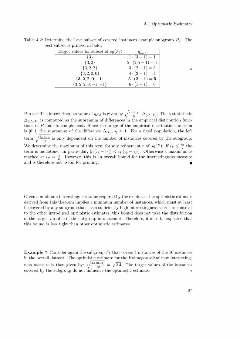
4.2 Optimistic Estimates
Table 4.2: Determine the best subset of covered instances example subgroup P2. Thebest subset is printed in bold.
Target values for subset of sg(P2) q1med
{3} 1 · (3− 1) = 1{3, 2} 2 · (2.5− 1) = 1{3, 2, 2} 3 · (2− 1) = 3{3, 2, 2, 0} 4 · (2− 1) = 4
{3,2,2,0,−1} 5 · (2− 1) = 5{3, 2, 2, 0,−1,−1} 6 · (1− 1) = 0
2
Proof The interestingness value of qKS is given by√
iP ·i¬Pi∅·∆(P,¬P ). The test statistic
∆(P,¬P ) is computed as the supremum of differences in the empirical distribution func-tions of P and its complement. Since the range of the empirical distribution functionis [0, 1] the supremum of the difference ∆(P,¬P ) ≤ 1. For a fixed population, the left
term√
iP ·i¬Pi∅
is only dependent on the number of instances covered by the subgroup.
We determine the maximum of this term for any refinement r of sg(P ): If iP ≤ i∅2 the
term is monotone. In particular, |r|(i∅ − |r|) < iP (i∅ − iP ). Otherwise a maximum isreached at iP = i∅
2 . However, this is an overall bound for the interestingness measureand is therefore not useful for pruning. �
Given a minimum interestingness value required by the result set, the optimistic estimatederived from this theorem implies a minimum number of instances, which must at leastbe covered by any subgroup that has a sufficiently high interestingness score. In contrastto the other introduced optimistic estimates, this bound does not take the distributionof the target variable in the subgroup into account. Therefore, it is to be expected thatthis bound is less tight than other optimistic estimates.
Example 7 Consider again the subgroup P1 that covers 4 instances of the 10 instancesin the overall dataset. The optimistic estimate for the Kolmogorov-Smirnov interesting-
ness measure is then given by:
√4·(10−4)
10 =√
2.4. The target values of the instancescovered by the subgroup do not influence the optimistic estimate. 2
87

4 Algorithms for Numeric Target Concepts
4.2.2.4 Rank-based Measures
Theorem 9 Two optimistic estimate bounds for the Mann-Whitney interestingness
measure qmw′(P ) =√
iPi¬P· (RPiP −
i∅+12 ) are given by:
oe1mw′(P ) =
∑c∈sg(P ),ρ(c)>
i∅+1
2
(ρ(c)− i∅ + 1
2
)
oemw′(P ) =√i+P (ρmaxP − i∅ + 1
2),
where ρ(c) is the rank of instance c in order of the target values, ρmaxP is the maximum
rank in the subgroup P and i+P = |{c ∈ sg(P ) | ρ(c) > i∅+12 }| is the number of instances
in the subgroup with a rank higher than the populations rank mean.
Proof It holds for all refinements r with a positive interestingness value, that
qmw′(P ) =
√iPi¬P
(RiP− i∅ + 1
2) ≤
√iP (RiP− i∅ + 1
2)
Since RiP
is the mean of the ranks within the subgroup and i∅+12 is the mean of the
ranks in the overall population, the right part of this equation is equal to the mean testfunction q0.5
mean if the target values are given by the ranks. Thus, we can transfer theupper bounds from Theorem 3. However, these bounds are substantially less tight forthis interestingness measure due to the initial estimation. �
Example 8 Consider again the subgroup P1 in a dataset of 10 instances and assumethat the 4 instances covered by the subgroup have the ranks ρ(c1) = 2, ρ(c2) = 3,ρ(c3) = 6 and ρ(c4) = 8. That is, the instance c1 has the second highest target value inthe dataset, c2 has the third highest target value, c3 has the sixth highest target valueand c4 has the eighth highest target value. Then, the optimistic estimates according tothe above theorem are given by:
oe1mw′(P1) =
∑c∈sg(P ),ρ(c)>
i∅+1
2
(ρ(c)− i∅ + 1
2
)= (6− 11
2) + (8− 11
2) = 3
oemw′(P1) =√i+P (ρmaxP − i∅ + 1
2) =√
2 · (8− 11
2) =√
2 · 2.5)
The first bound is tighter in this example and is therefore used as the overall bound foroptimistic estimate pruning. In doing so, specializations of the subgroup P1 have not tobe considered in the subgroup discovery algorithm, if the result set requires a minimuminterestingness score of more than 3. 2
88

4.2 Optimistic Estimates
Theorem 10 If there are no ties in the ranks, then an optimistic estimate for the area-
under-the-curve interestingness measure qauc(P ) =R¬P−
i¬P ·(i¬P+1)
2iP ·i¬P is given by:
oeauc(P ) =i∅ − ρminP
i∅ − 1,
where ρminP is the minimum rank for an instance in P .
Proof Due to the construction of the area-under-the-curve the best subset of sg(P )contains only one instance, which is the one with the lowest rank ρmin. The interesting-
ness of this refinement S is qauc(S) =R¬S−
i¬S(i¬S+1)
2iSi¬S
=(i∅+1)i∅
2−ρminP − i∅(i∅−1)
21·(i∅−1) =
i∅−ρminPi∅−1 �
Example 9 Consider again the subgroup P1 that covers instances with following rankswith respect to the target concept: ρ(c1) = 2, ρ(c2) = 3, ρ(c3) = 6 and ρ(c4) = 8 in adataset that consists of 10 instances. Then, the above theorem provides the optimisticestimate: oeauc(P ) = 10−2
9 = 89 . 2
4.2.3 Ordering-based Bounds
In order to apply pruning of the search tree more frequently in a search algorithm,a tight optimistic estimate is desired. However, the estimates presented above onlyprovide loose estimates in many cases. As an alternative, one can check all subsetsof the subgroups instances for the one with the best interestingness score in order toobtain a tighter upper bound. Unfortunately, this is not directly feasible, as there isan exponential number of possible refinements for each subgroup. In the following, twouseful properties of interestingness measures are defined that simplify the identificationof the best refinement and thus the induction of optimistic estimate bounds.
4.2.3.1 One-pass Estimates by Ordering
Definition 2 An interestingness measure q is one-pass estimable by ordering, if it holdsfor any subgroup P and any refinement r ⊆ sg(P ), that:
q(r) ≤ max(q(sdesc1 ), . . . , q(sdesciP
)),
where sdescj is the set of instances that consists of the j instances of sg(P ) with thehighest target values. 2
This property expresses that for these measures the interestingness, which is implied bya set of instances, always increases, if one of the instances is exchanged with anotherinstance that has a greater target value. It reduces the number of candidates for thebest refinement of a subgroup from 2iP to iP .
This motivates the following approach for subgroup discovery with numeric targetconcepts using such interestingness measures: In a preprocessing step, the instances in
89

4 Algorithms for Numeric Target Concepts
the database are sorted in descending order with respect to their target values. Whenevera subgroup is evaluated, instances are added one by one to the subgroup, starting withthe highest value. After each addition, the interestingness of the instance set is evaluated.The maximum of these interestingness values is used as a tight optimistic estimate. Indoing so, only a single pass over each subgroup is required. In most cases, the gainthrough additional pruning options by far exceeds the additional effort for computingthe bounds, as shown in the evaluation in Section 4.6.
Theorem 11 The interestingness measures qamean(P ) = iPa · (µP − µ∅) are one-pass
estimable by ordering.
Proof We consider any refinement r ⊆ sg(P ) and compare it to the instance set r∗ =sdesc|r| . This is the subset with the same number of covered instances as r, but the highest
target values contained in sg(P ): Then, |r∗| = |r| and µr∗ ≥ µr. It follows that accordingto a mean-based interestingness measure the refinement r∗ is at least as interesting as r:
qamean(r) = |r|a · (µr − µ∅)≤ |r∗|a · (µr∗ − µ∅)= qamean(r∗) �
Example 10 In a dataset with a mean target value of 50, the subgroup P3 cov-ers the instances sg(P ) = {c2, c3, c4, c5}. The target values for these instances areT (c2) = 75, T (c3) = 53, T (c4) = 12, T (c5) = 100. These instances are ordered accord-ing to their target value in order to generate the subsets sdescj : sdesc1 = {c5}, sdesc2 =
{c5, c2}, sdesc3 = {c5, c2, c3}, sdesc4 = {c5, c2, c3, c4}. For each of these subsets the scoreof the interestingness measure is computed. In this example, the mean test measureq0.5mean(P ) =
√iP · (µP − µ∅) is used. The resulting scores are:
q0.5mean(sdesc1 ) =
√1 · (100− 50) = 50
q0.5mean(sdesc2 ) =
√2 · (87.5− 50) ≈ 53
q0.5mean(sdesc3 ) =
√3 · (76− 50) ≈ 45
q0.5mean(sdesc3 ) =
√4 · (60− 50) = 20
The maximum of these interestingness score, in this case q0.5mean(sdesc2 ) ≈ 53, then defines
an optimistic estimate bound for the subgroup. This bound is tighter than the estimateswith closed form expressions presented in Theorem 2 and Theorem 4:
oe1mean(P3) = (100− 50) + (75− 50) + (53− 50) = 78
oeamean(P3) =√
3 · (100− 50) ≈ 85.6 2
Theorem 12 The z-score interestingness measure qz(P ) =√iP ·(µP−µ∅)
σ∅is one-pass es-
timable by ordering.
90

4.2 Optimistic Estimates
Proof This follows directly from Theorem 11 since qz(P ) is order equivalent withq0.5mean. �
Theorem 13 The median-based interestingness measures qamed(P ) = iPa · (medP −
med∅) are one-pass estimable by ordering.
Proof Analogously to Theorem 11, replacing the mean by the median. �
Theorem 14 The rank-based interestingness measures qmw(P ) and −qauc(P ) are one-pass estimable by ordering.
Proof For any refinement r with |r| = j, the sum of ranks gets maximized (or mini-mized, depending on the ordering of ranking) for sdescj , therefore q(sdescj ) ≥ q(r) for theseinterestingness measures. �
4.2.3.2 Two-pass Estimates by Ordering
For symmetric interestingness measures, which indicate increases as well as decreases ofthe target concept, the most interesting refinement potentially covers only instances withlow target values. Thus, symmetric measures are never one-pass estimable. However, abroadened definition of this property is applicable in this case:
Definition 3 An interestingness measure q is two-pass estimable by ordering, if it holdsfor any subgroup P and any refinement r ⊆ sg(P ) that:
q(r) ≤ max(q(sdesc1 ), . . . , q(sdesciP
), q(sasc1 ), . . . , q(sasciP)),
where sdescj is the set of instances that consists of the j instances of sg(P ) with thehighest target values and sascj is the set of j instances of sg(P ) that have the lowesttarget values. 2
Trivially, any interestingness measure, which is one-pass estimable by ordering, is alsotwo-pass estimable by ordering. For interestingness measures with this property, thebest subset of instances is found by traversing the current subgroup twice — once indescending and once in ascending order of the target values. In both passes, instancesare added one-by-one to the current set of instances. As before, after each addition theinterestingness score of the instance set is computed. The overall optimistic estimate isthen given by the maximum of all those scores. In doing so, 2 ·iP subsets of the instancesof the current subgroup are considered as candidates to find its best refinement.
Several symmetric interestingness measures, which identify increases as well as de-creases of the target value, fulfill this property:
Theorem 15 The symmetric mean based measures qaabs(P ) = ipa ·|µP−µ∅| are two-pass
estimable by ordering.
91

4 Algorithms for Numeric Target Concepts
Proof Consider any refinement r ⊆ sg(P ). Without loss of generality, let j = |r| bethe number of instances covered by r. If µr ≥ µ∅ then qa(s
descj ) ≥ qa(r) in analogy to
the proof of Theorem 11. Otherwise, µr < µ∅ and we can conclude that qa(sascj ) ≥ qa(r)
since |sascj | = |r| and µsasci≤ µr and therefore |µsascj
− µ∅| ≥ |µr − µ∅|. �
Example 11 As in the last example, let the subgroup P3 cover 4 instances with targetvalues T (c2) = 75, T (c3) = 53, T (c4) = 12, T (c5) = 100. As interestingness measure,any symmetric mean based measure is used. To compute the optimistic estimate forthis interestingness measure, the subsets sdescj are formed as in the previous example.Additionally, the subsets sascj are constructed using the ascending order of the targetvalues: sasc1 = {c4}, sasc2 = {c4, c3}, sasc3 = {c4, c3, c2}, sasc4 = {c4, c3, c2, c5} For each ofthese subset the score of the interestingness measure is computed and the maximum ofthese interestingness scores determines the optimistic estimate. 2
Theorem 16 The interestingness measure variance reduction qvr(P ) = iPi∅−iP
·(µP−µ∅)2
is two-pass estimable by ordering.
Proof For any refinement r ⊆ sg(P ) that covers j = |r| instances, it holds that (µP −µ∅)
2 ≤ max(
(µsdescj− µ∅)2, (µsascj
− µ∅)2)
. Thus, qvr(r) ≤ max(qvr(s
descj ), qvr(s
ascj ))
. �
4.2.3.3 Interestingness Measures not Estimable by Ordering
As shown before, many interestingness measures for numeric target concepts are one- ortwo pass estimable by ordering. Although these properties seem intuitive, they do notapply to all interestingness measures:
Theorem 17 The generic variance interestingness measure qasd(P ) = iPa · (σP − σ∅) is
not one-pass or two-pass estimable by order.
Proof Assume that the standard deviation in a dataset is overall σ∅ = 1 and thesubgroup P4 covers 3 instance with target values T (c1) = 10, T (c2) = 0, and T (c3) =−10. The subset r∗ with highest standard deviation and therefore the highest scoreaccording to q0
sd(P ) then consists of the two instances c1 and c3. The mean value for this
subset is µr∗ = 0 and its variance is sd2r∗ = (10−0)2+(0−(−10))2
2−1 = 200. The interestingness
score for this subset is then q0sd(r
∗) = 20 · 200 − 1 = 199, which is greater than theinterestingness score of all subsets sdescj or sascj . �
Theorem 18 The t-score interestingness measure qt(P ) =√iP ·(µP−µ∅)
σPis not one-pass
or two-pass estimable by order.
Proof Consider a dataset with µ∅ = 0 and a subgroup P within the dataset thatcontains four instances i1, . . . , i4 with the target values T (i1) = 20, T (i2) = 10, T (i3) =10 + ε, T (i4) = 0, ε � 0.1. Then the best refinement r∗ contains the instances i2and i3. The interestingness of r∗ approaches infinity if ε approaches 0. Thus, qt(r
∗) >max(qt(s
desci ), qt(s
asci )) for any i given a small ε. This contradicts the definition of one-
pass and two-pass estimability by ordering. �
92

4.2 Optimistic Estimates
The novel algorithm NumBSD , which is introduced later in this chapter, incorporatesthe presented ordering-based estimates in an efficient algorithm. However, these boundscan not be computed using arbitrary data structures, i.e., they can not be used incombination with FP-trees, cf. also Section 5.3.
4.2.4 Fast Bounds using Limited Information
This section presents a novel method to speed up the computation process by applyinga sequence of less precise upper bounds, which are computed during the evaluation ofa single subgroup. The bounds are determined by using only the refinements sdescj ofP , that is, the j instances in P with the highest target values. The section focusesexclusively on the probably most popular family of interestingness measures in thissetting, the generic mean-based interestingness measures qamean.
The main idea is as following: As before, instances are incorporated one-by-one indescending order of the target values into the evaluation of a subgroup. After eachinstance, the interestingness for the set sdescj of the already incorporated j instances is
computed. By definition, the maximum of all interestingness values q(sdescj ) is an opti-mistic estimate for interestingness measures, which are one-pass estimable by ordering.We now consider a certain point in time during this pass over the dataset, at which thefirst n instances have already been processed. At this point, it is guaranteed that thetarget values for all following instances in the subgroup are not greater than the targetvalue of the current case. This fact is used to determine an upper bound for all theinterestingness values q(sdescj ), which have not yet been computed: For all instances,which have not been visited yet, it is assumed that the target value of these instancesis equal to the target value of the instance, which was added last. By assuming greatertarget values, the computed interestingness value according to any generic mean-basedinterestingness measure qamean always increases, since the interestingness measure is one-pass estimable. Thus, we compute the maximum value that is obtained by adding anynumber of instances with the current target value. This forms an upper bound for theremaining interestingness values q(sdescj ), j > n. If this weaker upper bound already in-dicates that none of the refinements of the current subgroup (nor the current subgroupitself) will be added to the result set, then we can skip the rest of the evaluation of thissubgroup. Formally, this approach can be based on the following formal theorem:
Theorem 19 For a subgroup P , let sdescn ⊆ sg(P ) be the n instances with the highesttarget values. Furthermore, let σ =
∑c∈sdescn
T (c) be the sum of target values for sdescn
and θ the lowest target value for the instances in sdescn , that is, the n-th highest targetvalue in sg(P ). Then, an optimistic estimate for generic mean-based interestingnessmeasures qamean(P ) = iP
a · (µP − µ∅)(P ) is given by:
oeafast(P ) = max(qamean(sdesc1 ), . . . , qamean(sdescn ), oearemaining(P )
),
oearemaining(P, n) = iPa ·(σ + (iP − n) · θ
iP− µ∅
)
93

4 Algorithms for Numeric Target Concepts
Proof The theorem is proven by showing that for each subset r ⊆ sg(P ) the interest-ingness score is not higher than the provided optimistic estimate: qamean(P ) ≤ oeafast(P ).Since qamean(P ) is one-pass estimable, for each r the interestingness is lower than theinterestingness of the subset, which has the same number of instances, but covers theinstances with the highest target values: qamean(r) ≤ qamean(sdesc|r| ). Thus, the theorem
holds for all r with |r| ≤ n.
For all refinements r with |r| > n, it remains to show that qamean(sdesc|r| ) ≤ oeafast(P ). To
do so, the interestingness of sdescj for any j = n+x with x > 0, x ≤ xmax, xmax = iP −nis estimated. Let ck be the instance with the k-highest target value.
qamean(sdescj )(P ) = ja ·
(∑jk=1 T (ck)
j− µ∅
)
= (n+ x)a ·(∑n
k=1 T (ck) +∑x
k=n+1 T (ck)
n+ x− µ∅
)≤ (n+ x)a ·
(σ + x · θn+ x
− µ∅)
:= fa(x)
The inequality utilizes that the target values are ordered descending and it thereforeholds for k > n that T (ck) ≤ T (cn) = θ. The function fa(x) describes an upper boundfor the interestingness of the instance set sdescj that consists of x instances more than
the last evaluated instance set sdescn . Unfortunately, the size j of the instance set withthe maximum interestingness and the respective x value is not known. However, anupper bound for the interestingness of q(sdescj )(P ) is given by the maximum value offa(x). For this family of functions, it can be shown by computing the first and secondderivative that the maximum value is reached either at x = 0 or at x = xmax = iP − n.The formal proof is provided in the appendix of this chapter. This means that themaximum upper bound is reached, if either none or all remaining instances are addedto the last evaluated instance with an assumed target value of θ. For x = 0, thevalue of the function fa is equal to the interestingness score of the instance set sdescn :
fa(0) = (n+ 0)a ·(σ+0·θn+0 − µ∅
)= na · (µsdescn
− µP ) = qamean(sdescn ).
As a consequence it holds for all r ⊆ sg(P ) with |r| = j > n that
qamean(r) ≤ q(sdescj )
≤ fa(x)
≤ max (fa(0), fa(iP − n))
= max
(qamean(sdescn ), iP
a · (σ + (iP − n) · θiP
− µ∅))
≤ oeafast(P )
This proves the theorem. �
94

4.3 Data Representations
This theorem provides an upper bound for the interestingness score of all specializa-tions of a subgroup and also for the interestingness of the subgroup itself. It is basedonly on a part of the instances of a subgroup, that is, the ones with the highest targetvalues. Thus, the above estimates can be checked during an iteration over the subgroupinstances even before this iteration has finished. If after only a few instances the com-puted upper bound indicates that the subgroup itself and all its specializations do nothave a sufficient interestingness for the result set, the evaluation of the subgroup canbe stopped. In doing so the majority of the subgroup has not to be considered, thusspeeding up the subgroup discovery process. To the author’s knowledge, this is the firstapproach that uses optimistic estimates, which are based only on a part of a subgroup’sinstances.
Example 12 Again, the subgroup P1 is considered, which covers 4 instances with targetvalues T (c1) = 100, T (c2) = 75, T (c3) = 53, T (c4) = 12. The mean target value in theoverall dataset is µ∅ = 50. Additionally, it is assumed that a score of at least 150 iscurrently required by the result set using the impact interestingness measure q1
mean.For the evaluation of P1, instances are added one-by-one, starting with the instance c1,
since it has the highest target value. The interestingness value of a subgroup that coversonly this single instance is q(sdesc1 ) = 1 · (100 − 50) = 50. To compute the optimisticestimate oeafast(P1) after the first instance, additionally the value of oearemaining(P1) is
required. This is determined as iP1a ·(σ+(iP1
−n)·θiP1
− µ∅)
= 4 1 ·(
100+(4−1)·1004 − 50
)=
200. Since 200 exceeds the minimum required interestingness of 150, the evaluation ofP1 continues.
Next, the instance c2 is added, as it has the second highest target value. The corre-sponding interestingness value is q(sdesc2 ) = 2 · (87.5− 50) = 75. Additionally, the value
of oearemaining(P1) is updated: oearemaining(P1) = 41 ·(
175+(4−2)·754 − 50
)= 125. It fol-
lows that oeafast(P1) = max(q(sdesc1 ), q(sdesc2 ), oearemaining(P )
)= max(50, 75, 125) = 125
is an optimistic estimate for the subgroup P : P itself and all of its specializations areguaranteed to not have interestingness scores higher than 125. As the minimum re-quired interestingness value of the result set is 150, the evaluation of P can stop withoutconsidering the remaining instances c3 and c4. 2
The formula for the above bound requires the number of instances, which are coveredby a subgroup. This number might not yet be known during the evaluation iteration ofthe subgroup. However, a simple upper bound for the maximum number of instancesin a subgroup can be estimated, e.g., by the known number of instances covered by ageneralization of the subgroup.
4.3 Data Representations
In subgroup discovery, specialized data structures allow for the efficient computation ofsubgroup statistics. These are required to determine interestingness scores and optimisticestimates of subgroups. This section introduces adaptations of two data structures to the
95

4 Algorithms for Numeric Target Concepts
setting of subgroup discovery with numeric target concepts, that is, FP-trees and verticalbitset-based data structures. It primarily focuses on the most important interestingnessmeasures, that is, generic mean-based interestingness measures.
4.3.1 Adaptations of FP-trees
As described in detail in Section 3.3.3, the adapted FP-tree structure for subgroup dis-covery as proposed for the SD-Map algorithm [22] consists of nodes, which are connectedby two link structures, tree links and auxiliary links. The modifications for numeric tar-get concepts do not affect the link structures, but only exchanges the information that isstored in each node. For the binary case, an FP-tree node stores the number of instancesand the number of positive instances for the respective instance set. In the case of anumeric target concept and a mean-based interestingness measure, the sum of targetvalues and the instance count is stored instead. This enables the computation of themean target value of an instance set and thus allows for determining the interestingnessvalue. Using these adaptations for numeric target variables, the case of a binary targetis included as a special case, if the value of the target is set to 1 for true target conceptsand to 0 for false target concepts.
To efficiently compute the optimistic estimate presented above, additional informationis required, which is also stored in the tree nodes: To compute the optimistic estimateoe1mean presented in Theorem 2 one additional field is used, which is initialized with 0. For
each instance c corresponding to the node, the value max (0, T (c)− µ∅) is added to thisfield. As the other stored values, this field is propagated recursively, when conditionaltrees are built. In doing so, the value stored in this field of each node reflects the sum∑
c∈P :T (c)>µ∅(T (c) − µ∅), that is, the exact value of the optimistic estimate. Thus, the
optimistic estimate is directly available if pruning options are checked. Analogously, forthe optimistic estimate oeamean(P ) = pP
a · (TmaxP − µ∅), each node must keep track ofthe number of instances p, which have a target value greater than the population meantarget value, and the maximum target value corresponding to this node Tmax. Theseare propagated accordingly and allow for the efficient computation of these bounds.
Adaptations for other interestingness measures For other interestingness measures, dif-ferent kinds of information needs to be stored in the tree nodes:
To apply a variance-based interestingness measure such as the t-score measure qt(P ),in addition to the sum of values the sum of squared values needs to be stored to determinethe variance within the subgroup. This is discussed in detail in the context of generalizedFP-trees, see Chapter 5. Unfortunately, it is difficult to determine optimistic estimatesfor this function in general, see Section 4.2.
To compute the symmetric generic mean-based measures, no additional informationis required other than the sum of values and the frequency count of instances. In orderto determine optimistic estimates, it is required to additionally store the sum of targetvalues, which are below the population target mean, and the minimum target value.Similarly, for the variance reduction qvr(P ) the instance count and the overall sum oftarget values is required to compute the interestingness itself. For the computation
96

4.3 Data Representations
of optimistic estimate bounds, the sum of target values higher, resp. lower than thepopulation mean as well as the minimum and maximum target value is also required.
The generic median-based measures cannot be computed by applying an FP-tree-baseddata structure since more than one pass over the subgroup is required to compute therequired median statistics, cf. Chapter 5. The same applies to the Kolmogorov-Smirnovinterestingness measure qks.
To compute rank-based interestingness measures using a variation of FP-trees, theranks of instances must be determined in a preprocessing step. Afterwards, ranks replacethe original target values in the algorithm itself. In the FP-tree nodes, only the instancecount and the sum of ranks is stored and aggregated.
4.3.2 Adaptation of Bitset-based Data Structures
To adapt bitset-based, vertical data structures to numeric target settings and to theintroduced ordering-based bounds, two adaptations to the data structure in the binarysetting are necessary. First, the instances of the total population are initially sortedin descending order with respect to the target variable. The ordering allows for easycomputation of ordering-based optimistic estimate bounds. Analogously to the binarycase, a bitset of length i∅ is constructed for each selector in the search space, such thatthe i-th bit in each bitset is set to true, iff the instance with the i-th highest targetvalue is covered by the respective selector. For subgroups with conjunctive descriptions,a corresponding bitset is then computed by performing logical AND operations on thebitset of the respective selectors.
Second, the numeric target values are stored in an array in descending order. Thisreplaces the additional bitset used for the target concept in the binary case. The arrayof target values and the bitsets for the selectors correspond to each other via the positionof the instances, i.e., the target value of an instance, which is represented by the n-thbit of a bitset, is given at position n of the array of target values.
The computation of (for example) the mean value of a subgroup sel1 ∧ sel2, requiresone iteration over all bits, which are set to true in the bitset that corresponds to thissubgroup. For each bit, which is set to true, the respective target value of the arrayis added to a total sum and the count of instances is incremented. These statistics arethen used to compute the mean value.
Technically, each bitset is divided into words (e.g., of 32 or 64 bits), on which logicalboolean operations (such as OR and AND) can be applied very efficiently. For eachselector, the respective bitset is stored in a map for quick access.
The runtime requirement to sort a dataset with i∅ instances according to the targetvalues is in O(i∅ · log i∅). This is dominated by the search process in the subgroupdiscovery algorithm, unless the search space is very small in comparison to the number ofinstances in the dataset, i.e., |Σ| < log i∅. The construction of the bitset is accomplishedin one single pass through the database. The rest of the algorithm can then operate onthe generated data structures only and does not need further access to the database.The memory consumption for i∅ instances in the database and |S| selectors is thus givenby i∅ · (|S|+ 64) bits, if the numeric target values are stored with 64 bit precision.
97

4 Algorithms for Numeric Target Concepts
4.4 Algorithms for Subgroup Discovery with Numeric Targets
Next, two novel algorithms for efficient subgroup discovery are presented that utilize thetheoretical results of this chapter, that is, novel optimistic estimate bounds and datastructures. While both algorithms employ a similar enumeration strategy – depth-first-search with a one-level look-ahead – the algorithms differ fundamentally in the used datastructures: The SD-Map* algorithm, which is presented first, is based on adapted FP-trees. The algorithm NumBSD works on an adapted bitset-based data structure. Bothalgorithm exploit efficient strategies for optimistic estimate pruning based on the boundsderived in Section 4.2. Due to the employed data structures the SD-Map* algorithm islimited to bounds in closed form expressions. In contrast, the algorithm NumBSD canalso utilize ordering-based bounds, including the fast bounds presented in Section 4.2.4.
This section describes algorithm implementations for the generic mean-based interest-ingness measures. Solutions for other measures can be derived by slight modifications,as discussed in the previous sections.
4.4.1 The SD-Map* Algorithm
The SD-Map* algorithm is a novel algorithm for subgroup discovery with numeric targetconcepts. It improves its predecessor SD-Map [22] in several directions: While SD-Mapfocuses exclusively on binary targets, SD-Map* modifies the employed FP-tree datastructure in order to determine statistics of the numeric target concept as described inSection 4.3.1.
The statistics contained in the nodes of the FP-trees is not only used to computethe interestingness of subgroups, but also their optimistic estimates. In that direction,SD-Map* allows the incorporation of pruning based on the bounds in closed form ex-pressions, which have been presented in Section 4.2.2. Ordering-based bounds cannotbe applied since the ordering information is not captured by FP-tree representations,see Section 5.3 for a formal proof.
Pruning is applied in two different forms within the algorithm: First, selector pruningis performed in the recursive step, when a conditional FP-tree is built. A (conditioned)branch is omitted if the optimistic estimate for the conditioning selector is below thethreshold given by the k best subgroup qualities. Second, header pruning is used, when a(conditional) frequent pattern tree is constructed. Here, all the nodes with an optimisticestimate below the mentioned interestingness threshold can be omitted.
To maximize the efficiency of pruning, also the search strategy was slightly modified:Instead of the basic depth-first-search used in the SD-Map algorithm, SD-Map* appliesa depth-first strategy, similar to the DpSubgroup algorithm by Grosskreutz et al. [100].Reordering of the search space is performed by sorting of the header nodes: During theiteration over the candidate selectors for the recursive call, the selectors are reorderedaccording to their optimistic estimate value. In doing so, more promising selectors areevaluated first. In a top-k-approach, this helps to include high scoring subgroups earlyinto the result set in order to provide higher thresholds for more efficient pruning.
98

4.4 Algorithms for Subgroup Discovery with Numeric Targets
4.4.2 The NumBSD Algorithm
Although FP-tree-based approaches have shown excellent performance particularly withlarge datasets, they are not applicable for all interestingness measures. Additionally,they can not make use of ordering-based pruning schemes and the construction of aninitial FP-tree can require significant overhead, particularly if the search is limited toshort search depths. Therefore, we present the exhaustive subgroup discovery algorithmNumBSD as an alternative: It uses an efficient vertical, bitset-based data structure asdescribed in the previous section. As search strategy, NumBSD employs a depth-first-search approach with one level look-ahead, similar to the SD-Map* algorithm. Thealgorithm applies efficient pruning strategies, including ordering-based bounds and fastbounds, see Sections 4.2.3 and 4.2.4.
The algorithm NumBSD and its sub-procedures are shown in Algorithm 9. It firstinitializes the vertical data structures and then calls the main recursive function recurse.
This function consists of two parts. In the first part (lines 2-9) all direct specializa-tions, that is, all subgroups created by adding a single selector to the description of thecurrent subgroup, are considered. For these specializations the corresponding bitsets,the interestingness value and the optimistic estimates are computed. This is achievedefficiently in a single run through the subgroup by the method computeRefinement de-scribed below. If the interestingness value of a specialization is sufficiently high, then itis added to the result set. This potentially replaces a subgroup with a lower interest-ingness score and increases the minimum required interestingness score of the result set.Only if the optimistic estimate for a specialization exceeds the minimum interestingnessvalue of the result set, this refinement is also considered for the recursive search. In thesecond part of the function (lines 10-12), it calls itself recursively for these candidatesubgroups.
For the performance of the algorithm, an efficient computation of the bitset, theinterestingness score and the optimistic estimate of a refinement is essential. This isperformed in the function computeRefinement of Algorithm 9. First, an upper boundfor the maximum number of instances of a refinement is given by the number of instancesfor the current subgroup and for the additional selector. Each bitset technically consistsof words of 32 (respectively 64) bits. The bitset representing the instances of the spe-cialization spec is computed word by word by a logical AND between the bitset of thecurrent subgroup and the bitset of the new selector. Then, for each bit in this word,which is set to true (each instance of the refinement), the count and sum of target valuesare adjusted. Based on these values the interestingness score of the current part of therefinement is computed. When considering the i-th bit of the refinement, the interest-ingness is equal to q(sdesci ) for the refinement spec in the terminology of Theorem 11.Thus the maximum of the interestingness scores computed in this way determines a tightoptimistic estimate for the subgroup under evaluation. Since sdesciP
= sg(P ), the last ofthese scores is equal to the interestingness of the overall subgroup.
As a further improvement, the fast optimistic estimates as proposed in Theorem 19are checked after each word of the bitset. If neither this bound nor any of the alreadycomputed values q(sdesci ) are sufficiently high for the result set, then the evaluation of
99

4 Algorithms for Numeric Target Concepts
Algorithm 9 NumBSD algorithm
1: function NumBSD(maxDepth)2: Sort(allInstances) // sort w.r.t. target values3: TargetVal ← array of target values4: for all sel in allSelectors do5: bitsets(sel) ← createBitset(sel)
6: allT rue← new bitset, all bits set to 17: recurse(allTrue, ∅, allSelectors, maxDepth)
1: function recurse(currentBitset, currentDescription, remainingSels, maxDepth)2: nextSelectors← ∅3: for all sel in remainingSels do4: nextBitSet ← computeRefinement(currentSG ,sel)5: if nextBitSet.estimate > result .minQuality then6: nextBitsets(sel)← nextBitset7: nextSelectors← nextSelectors ∪ sel8: if nextBitSet .quality > result .minQuality then9: result .add (currentDescription ∪ sel)
10: if prefix.size < maxDepth then11: for all sel in nextSelectors do12: recurse(nextBitsets(sel), prefix ∪ sel, nextSelectors \ sel,maxDepth)
1: function computeRefinement(currentBitset, sel, minQualityThreshold)2: maxN ← Math.min(currentBitset, bitsets(sel).cardinality)3: n ← 04: sum ← 05: maxEstimate ← 0;6: refinement ← new bitset ()7: for all i = 0 to countWords (currentBitset) do8: refinement.word[i] ← currentBitset.word[i] AND bitsets(sel).word[i]9: for all each bit b in refinement.bitset.word[i], that is set to true do
10: n ← n+111: currentValue ← TargetVal [global position of b]12: sum ← sum + currentValue13: maxEstimate = max (maxEstimate, computeQuality (n, sum))
14: sumEstimateAtEnd = sum + currentValue · (maxN - n);15: maxOEatEnd = computeQuality (maxN, sumEstimateAtEnd)16: if (maxEstimate < minQuality ∧ maxOEatEnd < minQuality) then17: refinement.optEstimate = max (maxEstimate, maxOEatEnd)18: return refinement % exploit fast pruning bounds
19: return refinement
100

4.5 Evaluation
the current subgroup can stop. Since the subgroup itself and all of its generalizationwill not contribute to the result set, the exact values of the interestingness and theoptimistic estimate are not of interest anymore. Thus, parts of this computation canbe safely omitted using the fast bounds introduced previously. In the worst case, themethod computeRefinement requires one complete pass through the instances of thecurrent subgroup.
4.5 Evaluation
The benefits of the proposed improvements were evaluated in a wide range of experi-ments. The algorithms were implemented in the VIKAMINE 2 environment, see Chap-ter 8. Runtime experiments were performed on a standard office PC with a 2.2 GHzCPU and 2 GB RAM. Experiments, which count the number of evaluated candidates,were executed on additional machines since results are independent from the hardwareperformance.
The experiments used publicly available datasets from the UCI [13] and KEEL [9]data repositories. For nominal attributes, attribute-value pairs were used as selectors.Numeric attributes were discretized into ten intervals by equal-frequency discretization.No overlapping intervals were generated.
The first part of the evaluation was concerned with the effects of the introducedoptimistic estimate bounds. In this regard, also the influence of the result size wasinvestigated. The next part of experiments focused on the proposed data structures: Itcompared the runtimes of a simple depth-first-search algorithm, the NumBSD algorithmand the SD-Map* algorithm without the use of optimistic estimate pruning. Then, thefull algorithms with advanced data structures and optimistic estimate pruning wereevaluated in another series of experiments. Finally, the effects of the introduced fastbounds with limited information were investigated.
A focus of the experiments is on the generic mean-based interestingness measures sincethese are most popular in practical applications.
4.5.1 Effects of Optimistic Estimates
The first set of experiments evaluated the use of the introduced optimistic estimatebounds. In that direction, a subgroup discovery algorithm with depth-first-search, onelevel look-ahead, and no resorting was run for different interestingness measures anddifferent search depths (maximum numbers of selectors in a description). For the opti-mistic estimate pruning, a top-1 approach was applied, that is, it was searched only forthe one subgroup with the top score. Each run was executed three times in differentvariations: With no optimistic estimate pruning, with optimistic estimate pruning usingthe bounds in closed form, which were presented in Section 4.2.2, and with ordering-based optimistic estimate pruning, cf. Section 4.2.3. For each variation, the number ofevaluated candidates in recursive calls, that is, after the initial evaluation of the basicselectors (not including these), was counted.
101

4 Algorithms for Numeric Target Concepts
The respective results are summarized in Table 4.3, Table 4.4, and Table 4.5. Resultsfor the mean-based interestingness measures, see Table 4.3 and Table 4.4, are discussedfirst.
It can be observed that the number of required evaluations is reduced massively by ap-plying the presented optimistic estimate bounds. Even at low search depths, significantimprovements are achieved, often several orders of magnitude. The difference increaseseven further for higher search depths. In particular for ordering-based pruning, in manydatasets (almost) all further specializations can be pruned at depth two or three. In do-ing so, the required number of evaluations is not increased at all if the search is extendedto higher depths. In contrast, the unpruned size of the search size increases substantially.
Regarding different interestingness measures, optimistic estimate pruning has gener-ally less impact if the parameter a in the interestingness measures is lower (e.g., a = 0.5and a = 0.1), that is, if deviations of the target concept are more important. This can beexplained by the fact that even small subgroups can achieve high scores in this scenarioand thus the anti-monotonicity of the subgroup size is more difficult to exploit in thesecases. An exception is the extreme parameter a = 0, which is equivalent to the averageinterestingness measure: Since the best refinement of a subgroup is already determinedby the single instance with the highest target value, all subgroups that do not coverone of the instances with high target values can immediately be pruned by applying thenovel estimates of Theorem 4.
For the extreme settings a = 1 and a = 0, the bounds in closed form are tight,that is, they allow for the same amount of pruning as ordering-based bounds. For theintermediate settings a = 0.5 and a = 0.1, bounds in closed forms are considerably lessprecise. Therefore, often substantially more candidates must be evaluated in comparisonto ordering-based bounds. However, the optimistic estimate bounds in closed form stillreduce the number of required evaluations by orders of magnitude in comparison to theunpruned search space. Note that ordering-based bounds cannot be combined with alldata structures and come at higher computational costs.
Results for additional interestingness measures, are displayed in Table 4.5. As before,the maximum search depth was limited to d = 5. Similar to the mean-based interesting-ness measures, applying optimistic estimate bounds can lead to a massive reduction ofnecessary subgroup evaluations. However, the amount of the decrease of course is heavilyinfluenced by the utilized interestingness measure. For the symmetric mean-based mea-sure and the variance reduction, the number of evaluated candidates is often decreasedto less than 1000, if ordering-based optimistic estimates are applied. The optimistic es-timates in closed form are less tight, but still reduce the number of required evaluationsby more than an order of magnitude or more. Ordering-based bounds are also veryeffective for the other investigated interestingness measures, that is, the median-basedmeasure q0.5
med(P ), the Mann-Whitney measure qmw(P ), and the area-under-the-curveqauc(P ). Regarding optimistic estimates in closed form, even relatively simple to derivebounds can reduce the number of required candidate evaluations substantially, as in-dicated by the results for the Kolmogorov-Smirnov interestingness measure. The leasteffective bounds were by far the optimistic estimates for the Mann-Whitney, which onlywas able to prune about 40% of the candidates on average.
102

4.5 Evaluation
Tab
le4.
3:C
omp
aris
onof
pru
nin
gsc
hem
es,
i.e.
,n
op
run
ing
(Non
e),
ord
erin
g-b
ased
bou
nds
(Ord
er.)
and
bou
nds
incl
ose
dfo
rm(C
lose
d).
Th
eta
ble
pro
vid
esnu
mb
ers
ofsu
bgr
oup
s,w
hic
hh
adto
be
eval
uat
edin
ad
epth
-firs
t-se
arch
wit
hon
ele
vel
look
-ah
ead
and
no
reso
rtin
gu
sin
gth
em
ean
-bas
edin
tere
stin
gnes
sm
easu
rew
ith
the
par
amet
riza
tiona
=0.5
(not
cou
nti
ng
the
bas
icse
lect
ors)
.A
max
imu
mse
arch
dep
thd
=2,d
=3,
ord
=4
was
app
lied
asin
dic
ate
din
the
colu
mn
hea
der
.D
atas
etd
=2
d=
3d
=4
Non
eC
l.fo
rmO
rder
.N
on
eC
l.fo
rmO
rder
.N
on
eC
l.fo
rmO
rder
.ad
ult
s7,
408
2,7
54
228
181,7
81
17,2
89
733
1,7
56,6
27
48,8
52
1,3
63ai
lero
ns
59,3
406,4
86
193
4,1
75,4
23
43,4
38
680
166,9
62,6
85
234,2
92
1,9
86
auto
s20
,178
770
51
416,3
26
2,6
65
70
2,8
62,5
09
5,1
64
65b
reas
t-w
2,77
4317
19
36,8
31
412
19
124,3
10
427
19ce
nsu
s-kd
d*
87,7
254,2
54
995
6,5
44,2
76
39,1
99
5,0
72
73,3
74,1
93
262,1
79
19,0
12
com
mu
nit
ies*
708,
645
237,0
77
84
246,9
54,9
08
357,3
36
91
>2·1
09384,1
42
92
con
cret
ed
ata
2,34
61,6
56
123
35,5
31
2,4
40
130
130,1
38
2,5
05
131
cred
it-a
3,51
52,2
67
259
66,0
35
8,6
79
552
540,7
27
18,2
80
805
cred
it-g
3,98
62,5
02
258
98,3
57
14,9
33
577
1,2
41,6
92
44,8
98
818
dia
bet
es2,
277
2,0
15
96
39,4
85
4,6
63
101
206,1
21
5,1
13
102
elev
ator
s11
,175
8,1
28
100
453,2
50
20,2
50
184
11,4
35,3
41
38,6
57
296
flar
e1,
045
98
98
7,7
32
216
216
34,7
21
359
359
fore
stfi
res
6,24
1853
316
121,1
87
860
172
574,0
04
1,0
07
172
glas
s2,
761
72
16
34,2
28
81
17
93,9
52
81
17
hea
rt-c
2,00
01,7
54
353
33,4
51
6,3
86
712
233,0
43
11,4
29
930
hou
se10
,585
10,5
85
442
461,6
35
126,0
16
480
13,3
37,6
30
170,8
89
482
hou
sin
g6,
105
319
67
134,7
38
1,0
99
155
675,9
04
2,6
89
276
lett
er9,
971
5,0
48
9390,2
39
10,1
73
97,7
70,0
59
10,2
26
9m
v3,
003
58
35
59,6
89
60
35
722,5
32
60
35p
ole
5,77
82,1
41
657
181,2
80
12,8
66
3,7
85
3,8
13,3
84
50,3
15
18,8
16so
nar
175,
527
10,9
05
12
25,5
18,8
77
15,1
15
12
277,9
55,2
31
15,4
67
12sp
amb
ase
21,5
2718,5
30
6,8
48
1,2
96,9
13
314,8
07
48,5
26
46,4
68,9
24
4,3
24,1
21
641,2
96ti
cdat
a17
6,71
555,6
33
5,3
45
16,4
21,4
61
1,9
13,9
11
58,9
52
780,6
64,7
96
33,7
29,9
42
650,6
38
yeas
t1,
908
1,1
62
22
26,2
94
1,7
90
26
132,4
86
1,9
16
27
103

4 Algorithms for Numeric Target Concepts
Tab
le4.
4:C
omp
aris
onof
pru
nin
gsc
hem
es,
i.e.
,n
op
run
ing
(Non
e),
ord
erin
g-b
ased
bou
nd
s(O
rder
.)an
db
ou
nd
sin
close
dfo
rm(C
lose
d).
Th
eta
ble
pro
vid
esnu
mb
ers
ofsu
bgr
oup
sth
ath
adto
be
eval
uat
edin
ad
epth
-firs
t-se
arc
hw
ith
one
leve
llo
ok-a
hea
dan
dn
ore
sort
ing
(not
cou
nti
ng
the
bas
icse
lect
ors)
.T
he
sear
chw
asre
stri
cted
toa
maxim
um
of
5se
lect
ors
(on
ly4
for
the
two
dat
aset
sm
arke
dw
ith
a“*
”).
For
the
app
lied
mea
n-b
ased
inte
rest
ingn
ess
mea
sure
s,d
iffer
ent
par
amet
ersa
wer
eev
alu
ated
asin
dic
ated
inth
eco
lum
nh
ead
ers.
Ifn
op
run
ing
isap
pli
ed,
the
nu
mb
erof
requ
ired
can
did
ate
eval
uat
ion
sis
indep
end
ent
from
the
app
lied
inte
rest
ingn
ess
mea
sure
.D
atas
et1.0
0.5
0.1
0.0
Non
eC
lose
dO
rder
.C
lose
dO
rder
.C
lose
dO
rder
.C
lose
dO
rder
.ad
ult
s8,
503,
218
253
253
87,8
00
1,8
72
410,3
21
32,8
73
1,2
52
1,2
52
aile
ron
s98
4,28
9,40
54,2
98
4,2
98
912,2
56
4,3
84
46,0
81,3
83
148,8
30
1,4
70
1,4
70
auto
s12
,316
,190
17
17
8,3
47
66
52,7
64
1,8
84
134
134
bre
ast-
w21
9,99
312
12
427
19
6,4
13
963
132
132
cen
sus-
kd
d*
73,3
74,1
931,8
15
1,8
15
262,1
79
19,0
12
3,5
76,5
14
145,3
15
1,5
54
1,5
54
com
mu
nit
ies*
>2·1
0922
22
384,1
42
92
22,5
81,5
58
79,1
87
2,2
48
2,2
48
con
cret
ed
ata
209,
041
19
19
2,5
32
131
3,9
36
707
457
457
cred
it-a
2,23
1,11
8277
277
26,3
58
940
17,1
05
867
777
777
cred
it-g
8,38
9,27
1364
364
88,8
83
906
84,2
27
383
319
319
dia
bet
es35
0,46
617
17
5,1
13
102
2,0
08
316
342
342
elev
ator
s12
1,98
3,85
962
62
54,6
77
388
214,7
93
2,3
89
1,1
33
1,1
33
flar
e10
1,94
629
29
446
446
1,4
97
1,4
97
55
fore
stfi
res
1,20
9,24
230
30
1,0
90
172
875
164
161
161
glas
s14
1,71
413
10
81
17
529
87
147
147
hea
rt-c
823,
995
224
224
14,0
86
975
5,9
42
516
357
357
hou
se17
3,76
8,45
021
21
182,5
83
482
465,2
28
13,4
24
769
769
hou
sin
g1,
554,
972
43
43
4,8
85
387
4,0
11
273
127
129
lett
er69
,157
,431
88
10,2
26
9183,3
79
3,4
09
988
990
mv
5,54
2,94
334
29
60
35
2,2
62
34
1,4
99
1,4
99
pol
e47
,553
,142
48,0
77
48,0
77
144,3
53
72,8
51
650,3
49
146,1
75
270
270
son
ar1,
737,
064,
885
12
12
15,5
21
12
156,6
47
1,2
53
1,2
08
1,2
08
spam
bas
e1,
045,
755,
337
2,7
41,0
42
2,7
41,0
42
44,6
63,3
01
6,7
26,0
31
11,3
81,1
17
2,9
23,0
91
878
878
ticd
ata
1,25
4,39
5,63
21,7
83,6
51
1,7
83,6
51
249,7
36,0
31
5,6
58,5
23
288,2
05,2
79
6,3
70,2
65
61
61
yeas
t29
1,04
223
23
1,9
41
27
3,1
90
259
217
217
104
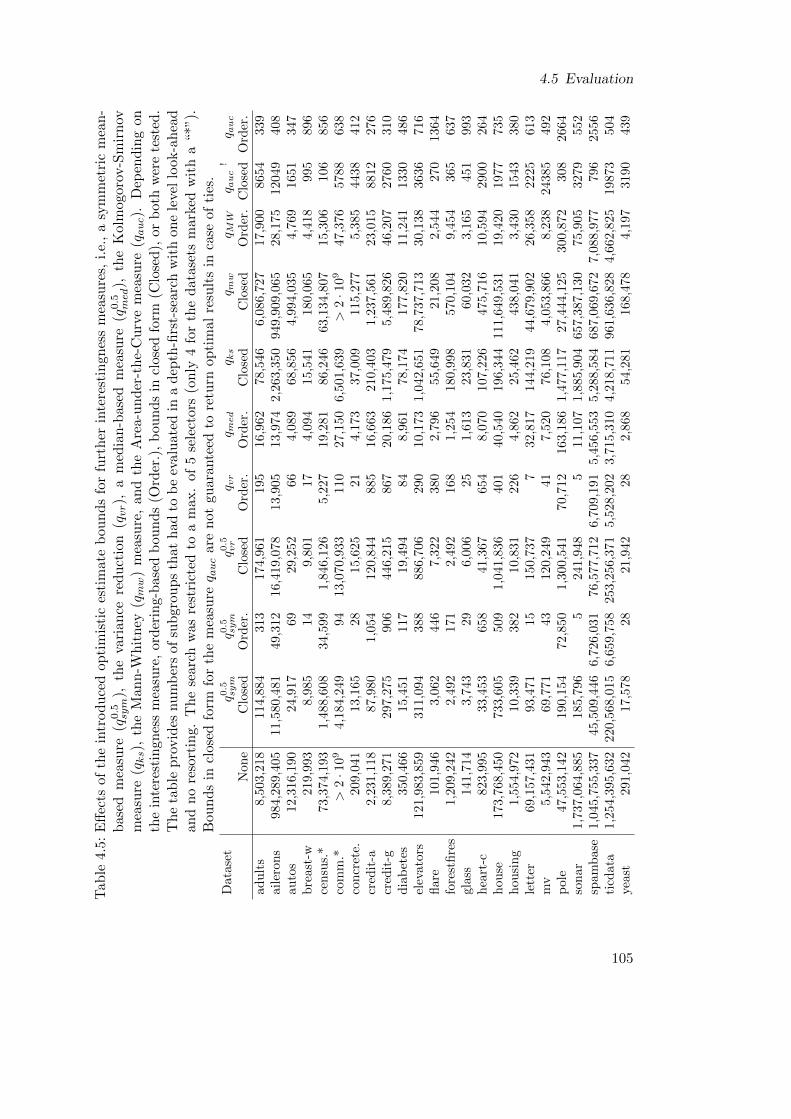
4.5 Evaluation
Tab
le4.
5:E
ffec
tsof
the
intr
od
uce
dop
tim
isti
ces
tim
ate
bou
nd
sfo
rfu
rth
erin
tere
stin
gnes
sm
easu
res,
i.e.
,a
sym
met
ric
mea
n-
bas
edm
easu
re(q
0.5sym
),th
eva
rian
cere
du
ctio
n(qvr),
am
edia
n-b
ased
mea
sure
(q0.5med
),th
eK
olm
ogor
ov-S
mir
nov
mea
sure
(qks),
the
Man
n-W
hit
ney
(qmw
)m
easu
re,
and
the
Are
a-u
nd
er-t
he-
Cu
rve
mea
sure
(qauc).
Dep
end
ing
on
the
inte
rest
ingn
ess
mea
sure
,or
der
ing-
bas
edb
oun
ds
(Ord
er.)
,b
oun
ds
incl
osed
form
(Clo
sed
),or
bot
hw
ere
test
ed.
Th
eta
ble
pro
vid
esnu
mb
ers
ofsu
bgr
oup
sth
ath
adto
be
eval
uat
edin
ad
epth
-firs
t-se
arch
wit
hon
ele
vel
look-a
hea
dan
dn
ore
sort
ing.
Th
ese
arch
was
rest
rict
edto
am
ax.
of5
sele
ctor
s(o
nly
4fo
rth
ed
atas
ets
mar
ked
wit
ha
“*”).
Bou
nd
sin
clos
edfo
rmfo
rth
em
easu
req auc
are
not
guar
ante
edto
retu
rnop
tim
alre
sult
sin
case
ofti
es.
Dat
aset
q0.5
sym
q0.5
sym
q0.5
vr
q vr
q med
q ks
q mw
q MW
q auc
!q a
uc
Non
eC
lose
dO
rder
.C
lose
dO
rder
.O
rder
.C
lose
dC
lose
dO
rder
.C
lose
dO
rder
.ad
ult
s8,
503,
218
114,
884
313
174,9
61
195
16,9
62
78,5
46
6,0
86,7
27
17,9
00
8654
339
aile
ron
s98
4,28
9,40
511
,580
,481
49,3
12
16,4
19,0
78
13,9
05
13,9
74
2,2
63,3
50
949,9
09,0
65
28,1
75
12049
408
auto
s12
,316
,190
24,9
1769
29,2
52
66
4,0
89
68,8
56
4,9
94,0
35
4,7
69
1651
347
bre
ast-
w21
9,99
38,
985
14
9,8
01
17
4,0
94
15,5
41
180,0
65
4,4
18
995
896
cen
sus.
*73
,374
,193
1,48
8,60
834,5
99
1,8
46,1
26
5,2
27
19,2
81
86,2
46
63,1
34,8
07
15,3
06
106
856
com
m.*
>2·1
09
4,18
4,24
994
13,0
70,9
33
110
27,1
50
6,5
01,6
39
>2·1
0947,3
76
5788
638
con
cret
e.20
9,04
113
,165
28
15,6
25
21
4,1
73
37,0
09
115,2
77
5,3
85
4438
412
cred
it-a
2,23
1,11
887
,980
1,0
54
120,8
44
885
16,6
63
210,4
03
1,2
37,5
61
23,0
15
8812
276
cred
it-g
8,38
9,27
129
7,27
5906
446,2
15
867
20,1
86
1,1
75,4
79
5,4
89,8
26
46,2
07
2760
310
dia
bet
es35
0,46
615
,451
117
19,4
94
84
8,9
61
78,1
74
177,8
20
11,2
41
1330
486
elev
ator
s12
1,98
3,85
931
1,09
4388
886,7
06
290
10,1
73
1,0
42,6
51
78,7
37,7
13
30,1
38
3636
716
flar
e10
1,94
63,
062
446
7,3
22
380
2,7
96
55,6
49
21,2
08
2,5
44
270
1364
fore
stfi
res
1,20
9,24
22,
492
171
2,4
92
168
1,2
54
180,9
98
570,1
04
9,4
54
365
637
glas
s14
1,71
43,
743
29
6,0
06
25
1,6
13
23,8
31
60,0
32
3,1
65
451
993
hea
rt-c
823,
995
33,4
53658
41,3
67
654
8,0
70
107,2
26
475,7
16
10,5
94
2900
264
hou
se17
3,76
8,45
073
3,60
5509
1,0
41,8
36
401
40,5
40
196,3
44
111,6
49,5
31
19,4
20
1977
735
hou
sin
g1,
554,
972
10,3
39382
10,8
31
226
4,8
62
25,4
62
438,0
41
3,4
30
1543
380
lett
er69
,157
,431
93,4
7115
150,7
37
732,8
17
144,2
19
44,6
79,9
02
26,3
58
2225
613
mv
5,54
2,94
369
,771
43
120,2
49
41
7,5
20
76,1
08
4,0
53,8
66
8,2
38
24385
492
pol
e47
,553
,142
190,
154
72,8
50
1,3
00,5
41
70,7
12
163,1
86
1,4
77,1
17
27,4
44,1
25
300,8
72
308
2664
son
ar1,
737,
064,
885
185,
796
5241,9
48
511,1
07
1,8
85,9
04
657,3
87,1
30
75,9
05
3279
552
spam
bas
e1,
045,
755,
337
45,5
09,4
466,7
26,0
31
76,5
77,7
12
6,7
09,1
91
5,4
56,5
53
5,2
88,5
84
687,0
69,6
72
7,0
88,9
77
796
2556
ticd
ata
1,25
4,39
5,63
222
0,56
8,01
56,6
59,7
58
253,2
56,3
71
5,5
28,2
02
3,7
15,3
10
4,2
18,7
11
961,6
36,8
28
4,6
62,8
25
19873
504
yeas
t29
1,04
217
,578
28
21,9
42
28
2,8
68
54,2
81
168,4
78
4,1
97
3190
439
105

4 Algorithms for Numeric Target Concepts
Overall, the reduction of required candidate evaluations was massive for almost allinterestingness measures and datasets. This clearly shows the use of the introducedoptimistic estimate bounds for diverse interestingness measures. The remainder of theevaluation will focus on the most popular measures, that is, differently parametrizedmean-based interestingness measures.
4.5.2 Influence of the Result Set Size
Top-k subgroup discovery aims at finding the best k subgroups according to the choseninterestingness measure. Optimistic estimate pruning exploits that the specializationsof the current subgroup can be guaranteed to receive a lower score than the best ksubgroups found so far. Therefore, the thresholds that are utilized for pruning increaseslower, if more subgroups are included in the result set. As a consequence, pruning canbe applied less often and more candidate subgroups must be explored.
The influence of the result set size on the number of required subgroup evaluationswas studied in another series of experiments. Table 4.6 shows the number of candidateevaluations, which were performed in a depth-first-search with one level look-ahead usingthe mean-based interestingness measure q0.5
mean(P ) for different sizes k of the result set.The search depth was limited to five. For pruning, ordering-based bounds were applied.
It can be seen that for all sizes of the result set, the number of evaluated candidatesis still by orders of magnitudes smaller than in a search without optimistic estimates.Nonetheless, the size of the result set has a noteworthy impact on the amount of pruningin many datasets: As expected, the number of evaluated candidates increases withthe size of the result set. Fortunately, the (relative) increase is much more moderatefor datasets, which require large numbers of subgroup evaluations even with optimisticestimate pruning, see the datasets spambase and ticdata. This can be explained by thefact that the large amount of evaluations is required, because the dataset contains manysubgroups with similar scores according to the applied interestingness measure. In thiscase, however, the threshold for the result set, that is, the minimum interestingness scorein the result set, is also less influenced by the size of the result set k. Overall, optimisticestimate pruning is clearly also very useful for larger result set sizes.
4.5.3 Influences of Data Structures
In the next series of experiments, the effects of different data structures were investigated.In that direction, the runtimes of the presented algorithms without applying optimisticestimate pruning were measured. This was performed for the NumBSD algorithm, whichis based on a bitset-based representation, as well as for the SD-Map* algorithm, whichis based on FP-trees. For comparison, the task was also solved by a trivial depth-first-search without any specialized data structure (repeated checking of the selectionexpressions in memory). Since no optimistic estimate bounds are exploited, the runtimewas (almost) independent from the applied interestingness measure and size of the resultset k, see also Section 5.5.1. The experiments were performed with different maximum
106

4.5 Evaluation
Table 4.6: Comparison of candidate evaluations for different sizes of the result set kif ordering-based optimistic estimate pruning is applied. As interestingnessmeasure, the mean test function q0.5
mean was used. The maximum search depth(maximum number of selectors in a description) was limited to d = 5.
Dataset No Pruning k = 1 k = 10 k = 100adults 8,503,218 1,872 4,793 21,854ailerons 984,289,405 4,384 5,440 18,935autos 12,316,190 66 291 4,283breast-w 219,993 19 178 3,751census-kdd* 73,374,193 19,012 22,474 42,815communities* > 2 · 109 92 1,266 32,845concrete data 209,041 131 866 4,294credit-a 2,231,118 940 6,241 18,982credit-g 8,389,271 906 8,703 24,604diabetes 350,466 102 2,971 8,002elevators 121,983,859 388 2,408 8,563flare 101,946 446 1,210 3,062forestfires 1,209,242 172 330 2,128glass 141,714 17 360 4,691heart-c 823,995 975 4,248 9,203house 173,768,450 482 4,302 27,033housing 1,554,972 387 688 81,706letter 69,157,431 9 1,098 20,229mv 5,542,943 35 2,072 9,629pole 47,553,142 72,851 108,189 3,416,279sonar 1,737,064,885 12 2,094 12,706spambase 1,045,755,337 6,726,031 6,849,488 6,861,101ticdata 1,254,395,632 5,658,523 5,710,867 6,215,858yeast 291,042 27 660 3,001
107

4 Algorithms for Numeric Target Concepts
Tab
le4.
7:C
omp
aris
onof
dat
ast
ruct
ure
s:T
he
tab
lesh
ows
the
runti
mes
inse
con
ds
ofsi
mp
led
epth
-firs
t-se
arc
h(S
imp
le),
Nu
mB
SD
(BS
D),
and
SD
-Map*
(SD
M)
wit
hou
topti
mis
tic
esti
mate
pru
nin
gfo
rd
iffer
ent
maxim
um
searc
hd
epth
sd.
Her
e,re
sult
sar
esh
own
for
the
inte
rest
ingn
ess
mea
sureq0.5mean,
bu
tre
sult
sar
eve
rysi
mil
ar
for
all
ap
pli
cab
lein
tere
stin
gnes
sm
easu
res.
Dat
aset
inst
ance
sd
=2
d=
3d
=4
d=
5d
=6
Sim
ple
BS
DS
DM
Sim
ple
BS
DS
DM
BS
DS
DM
BS
DS
DM
BS
DS
DM
adu
lts
3256
198
.01.5
4.3
3068.8
4.5
7.5
24.6
16.3
103.8
42.5
300.5
86.3
aile
ron
s13
750
394.
71.5
47.5
>4
h38.4
268.5
1009.0
1748.6
>4
h10
554.0
>4
h>
4h
auto
s20
51.
3<
0.1
0.3
41.4
0.6
1.7
4.3
7.5
20.6
36.3
75.6
145.0
bre
ast-
w69
90.
5<
0.1
0.1
7.5
0.1
0.1
0.2
0.2
0.3
0.4
0.5
0.5
cen
sus-
kd
d19
9523
8465
.747.2
223.4
>4
h533.2
1039.1
10470.0
5436.0
>4
h>
4h
>4
h>
4h
com
mu
nit
ies
1994
332.
73.3
482.3
>4
h567.3
10505.1
>4
h>
4h
>4
h>
4h
>4
h>
4h
con
cret
ed
ata
1030
0.6
<0.
10.1
9.7
0.1
0.2
0.2
0.3
0.4
0.5
0.4
0.5
cred
it-a
690
0.8
<0.
10.2
16.4
0.2
0.7
1.0
2.2
4.1
6.6
10.8
14.8
cred
it-g
1000
1.4
<0.
10.7
36.2
0.3
3.0
3.1
11.6
18.8
40.8
77.5
128.8
dia
bet
es76
80.
4<
0.1
0.1
7.4
0.1
0.2
0.3
0.4
0.5
0.5
0.6
0.6
elev
ator
s16
599
49.2
0.5
9.7
2198.8
5.6
28.9
83.8
96.4
672.1
309.0
2627.7
887.0
flar
e10
660.
4<
0.1
0.1
3.2
<0.
10.1
0.1
0.2
0.3
0.4
0.7
0.8
fore
stfi
res
517
1.1
<0.
10.2
27.4
0.2
0.5
0.9
1.3
2.0
2.9
3.4
4.4
glas
s21
40.
2<
0.1
<0.1
2.5
0.1
0.1
0.1
0.2
0.2
0.3
0.3
0.3
hea
rt-c
303
0.2
<0.
10.1
3.7
0.1
0.2
0.4
0.7
1.3
1.8
2.7
3.4
hou
se22
784
70.1
0.8
16.9
3077.3
7.7
51.9
131.6
157.2
1149.7
464.3
3565.7
1060.1
hou
sin
g50
60.
8<
0.1
0.2
19.3
0.2
0.5
1.0
1.4
2.5
3.5
4.6
6.3
lett
er20
000
54.1
0.7
10.6
2157.8
5.3
31.5
64.0
92.5
436.6
275.2
1455.9
601.3
mv
4076
831
.40.8
5.1
605.7
2.2
8.2
13.5
14.3
76.0
27.5
196.7
44.6
pol
e14
998
25.0
0.5
7.1
762.1
4.2
27.2
47.4
112.6
430.7
447.8
2894.4
1725.9
son
ar20
89.
50.5
8.5
1480.1
28.4
100.9
353.1
780.2
2971.2
9084.8
>4
h>
4h
spam
bas
e46
0125
.40.5
30.6
1650.4
11.9
287.0
266.8
2521.1
4626.0
>4
h>
4h
>4
hti
cdat
a58
2224
4.6
2.0
155.2
>4
h91.0
2018.7
3414.8
>4
h>
4h
>4
h>
4h
>4
hye
ast
1484
0.8
<0.
10.1
11.3
0.1
0.2
0.3
0.4
0.5
0.7
0.7
0.7
108

4.5 Evaluation
search depths d. Table 4.7 displays representative results for the measure q0.5mean and a
result set size of k = 1.
The results show that both introduced data structures – the bitset-based structure aswell as the FP-tree-based representation – substantially outperform the trivial approach.A direct comparison between the two approaches is more difficult: For lower searchdepths (d = 2, 3, 4), bitset-based structures enable faster runtimes than FP-trees. Thedifferences reach an order of magnitude for some datasets, e.g., for the communities andspambase datasets. For higher search depths (d = 5, 6), the results are more ambiguous:For some datasets the bitsets perform better, for some they perform worse than FP-trees.In particular, for datasets with a high instance count, the FP-tree-based approach areable to finish the tasks fast. In the census-kdd dataset, which is the largest tested dataset(in terms of instances), FP-trees perform better than bitsets already at a search depthof 4. This can be explained by the fact that the FP-trees achieve a better compressionof the data in datasets with a high instance count.
In summary, FP-trees are the data structure of choice if the dataset contains manyinstances, and if the maximum allowed number of selectors in a description is large. Incontrast, bitsets are preferred if the search is restricted to low search depths, or if theinstance count is comparatively low.
For some interestingness measure, it is not possible to derive optimistic estimatebounds, e.g., for generic variance-based measures or the t-score. Therefore, the run-times of the algorithms without optimistic estimate pruning shown in Table 4.7 reflectthe actual algorithm runtimes for these measures.
4.5.4 Runtimes of the Full Algorithms
Another series of experiments compared the runtimes of the full algorithms. Exemplaryresults of these evaluations are shown in Table 4.8 and Table 4.9. Experiments displayedin Table 4.8 utilized different interestingness measures and fixed search depth of d = 5.In contrast, experiments shown in Table 4.9 employed the fixed interestingness measureq0.5mean, but a variable search depth.
Results in Table 4.8 indicate that for a search depth of five, the application of opti-mistic estimate bounds leads to a substantial reduction of runtimes in comparison to thevariations without optimistic estimate pruning in almost all cases, cf. Table 4.7. Thebiggest improvements can be observed for the interestingness measures q1
mean and q0mean.
This corresponds the respective reduction in necessary candidate evaluations, see Ta-ble 4.4. Although the applied pruning bounds are in theory tighter for the NumBSDalgorithm, the speedups are often larger for the SD-Map* algorithm. This has tworeasons: First, pruning in SD-Map* is exploited twice, as header pruning and as se-lector pruning when conditional trees are built. Since the size of the conditional treesis reduced by pruning, not only less candidate evaluations are required with optimisticestimates, but each candidate evaluation also takes less time to compute. Second, thecomputation of the ordering-based bounds in NumBSD is more costly in itself. In onesingle experiment with unfavorable pruning properties, the computational costs for de-termining the bounds in this algorithm outweighed the use of pruning, that is, for the
109

4 Algorithms for Numeric Target Concepts
Tab
le4.
8:C
omp
aris
onof
the
full
algo
rith
ms:
Th
eta
ble
show
sth
eru
nti
mes
inse
con
ds
for
Nu
mB
SD
(BS
D)
an
dfo
rS
D-
Map*
(SD
M)
wit
hall
pru
nin
gopti
on
sen
abl
edfo
rd
iffer
ent
inte
rest
ingn
ess
mea
sure
s.T
he
searc
hw
as
lim
ited
toa
max
imu
mse
arch
dep
thofd
=5.
Th
efi
rst
two
colu
mn
ssh
owre
sult
sof
the
algo
rith
ms
wit
hou
topti
mis
tic
esti
mate
pru
nin
gfo
rco
mp
aris
on.
Dat
aset
No
Pru
nin
gq1 m
ean
q0.5
mean
q0.1
mean
q0 mean
BS
DS
DM
BS
DS
DM
BS
DS
DM
BS
DS
DM
BS
DS
DM
adu
lts
103.
842.5
0.8
2.3
11.1
6.1
19.7
14.1
1.3
2.5
aile
ron
s>
4h
10554.0
6.0
1.7
45.3
17.7
95.5
3345.9
0.6
147.0
auto
s20
.636.3
<0.1
<0.1
<0.1
0.1
<0.1
0.3
<0.1
<0.1
bre
ast-
w0.
30.4
<0.1
<0.1
<0.1
<0.1
<0.1
<0.1
<0.1
<0.1
cen
sus-
kd
d>
4h
>4
h53.3
52.6
5184.3
1280.5
14399.2
5795.2
35.0
52.1
com
mu
nit
ies
>4
h>
4h
0.1
0.9
0.1
4.3
2.0
108.0
0.3
0.9
con
cret
ed
ata
0.4
0.5
<0.1
<0.1
<0.1
<0.1
<0.1
0.1
<0.1
<0.1
cred
it-a
4.1
6.6
<0.1
<0.1
0.1
0.2
<0.1
0.2
<0.1
<0.1
cred
it-g
18.8
40.8
<0.1
0.1
0.2
0.9
0.1
0.9
<0.1
0.1
dia
bet
es0.
50.5
<0.1
<0.1
<0.1
<0.1
<0.1
<0.1
<0.1
<0.1
elev
ator
s67
2.1
309.0
0.2
0.9
1.0
2.4
1.9
4.1
0.3
0.9
flar
e0.
30.4
<0.1
<0.1
0.1
<0.1
0.1
<0.1
<0.1
<0.1
fore
stfi
res
2.0
2.9
<0.1
<0.1
<0.1
<0.1
<0.1
<0.1
<0.1
<0.1
glas
s0.
20.3
<0.1
<0.1
<0.1
<0.1
<0.1
<0.1
<0.1
<0.1
hea
rt-c
1.3
1.8
<0.1
<0.1
<0.1
0.1
<0.1
0.1
<0.1
<0.1
hou
se11
49.7
464.3
0.2
1.5
0.8
6.1
1.5
7.3
0.6
1.3
hou
sin
g2.
53.5
<0.1
<0.1
<0.1
<0.1
<0.1
<0.1
<0.1
<0.1
lett
er43
6.6
275.2
0.1
1.3
0.2
3.9
0.7
10.5
0.5
1.5
mv
76.0
27.5
1.0
1.7
1.9
1.4
0.9
2.8
0.9
1.6
pol
e43
0.7
447.8
26.8
1.6
263.0
38.6
186.8
81.0
0.3
2.5
son
ar29
71.2
9084.8
<0.1
<0.1
<0.1
0.1
<0.1
0.4
<0.1
<0.1
spam
bas
e46
26.0
>4
h692.9
609.5
7657.5
4269.1
3319.2
1900.3
0.2
151.2
ticd
ata
>4
h>
4h
820.4
56.9
12686.5
>4
h5588.2
>4
h0.1
1.0
yeas
t0.
50.7
<0.1
<0.1
<0.1
0.1
<0.1
0.1
<0.1
<0.1
110

4.5 Evaluation
Tab
le4.
9:C
omp
aris
onof
the
full
algo
rith
ms:
Th
eta
ble
show
sth
eru
nti
mes
inse
con
ds
ofN
um
BS
D(B
SD
),an
dS
D-
Map*
(SD
M)
wit
hall
pru
nin
gopti
on
sen
abl
edfo
rd
iffer
ent
max
imu
mse
arch
dep
thsd.
As
inte
rest
ingn
ess
mea
sure
,th
em
ean
testq0.5mean
was
use
d.
Dat
aset
d=
2d
=3
d=
4d
=5
d=
6B
SD
SD
MB
SD
SD
MB
SD
SD
MB
SD
SD
MB
SD
SD
Mad
ult
s2.
53.7
5.0
4.3
8.4
5.1
11.1
6.1
12.5
7.0
aile
ron
s3.
14.6
7.9
5.8
20.9
9.1
45.3
17.7
78.4
41.3
auto
s<
0.1
<0.1
<0.1
<0.1
<0.1
<0.1
<0.1
0.1
<0.1
0.1
bre
ast-
w<
0.1
<0.1
<0.1
<0.1
<0.1
<0.1
<0.1
<0.1
<0.1
<0.1
cen
sus-
kd
d92
.296.6
353.6
199.1
1490.7
462.8
5184.3
1280.5
>4
h3469.5
com
mu
nit
ies
0.2
4.0
0.2
4.0
0.2
4.1
0.1
4.3
0.2
4.4
con
cret
ed
ata
<0.
1<
0.1
<0.1
<0.1
<0.1
<0.1
<0.1
<0.1
<0.1
<0.1
cred
it-a
0.1
0.1
0.1
0.1
0.1
0.2
0.1
0.2
0.1
0.2
cred
it-g
0.1
0.3
0.1
0.5
0.2
0.7
0.2
0.9
0.2
1.0
dia
bet
es<
0.1
<0.1
<0.1
<0.1
<0.1
<0.1
<0.1
<0.1
<0.1
<0.1
elev
ator
s0.
62.1
0.8
2.2
0.9
2.2
1.0
2.4
1.1
2.3
flar
e<
0.1
<0.1
0.1
<0.1
0.1
<0.1
0.1
<0.1
0.1
<0.1
fore
stfi
res
<0.
1<
0.1
<0.1
<0.1
<0.1
<0.1
<0.1
<0.1
<0.1
<0.1
glas
s<
0.1
<0.1
<0.1
<0.1
<0.1
<0.1
<0.1
<0.1
<0.1
<0.1
hea
rt-c
<0.
1<
0.1
<0.1
0.1
<0.1
0.1
<0.1
0.1
<0.1
0.1
hou
se0.
75.3
0.7
5.5
0.7
5.6
0.8
6.1
0.7
5.6
hou
sin
g<
0.1
<0.1
<0.1
<0.1
<0.1
<0.1
<0.1
<0.1
<0.1
0.1
lett
er0.
23.7
0.2
3.8
0.2
3.8
0.2
3.9
0.2
3.8
mv
1.7
1.4
1.7
1.2
1.7
1.2
1.9
1.4
1.7
1.3
pol
e3.
52.7
18.6
5.9
79.8
14.7
263.0
38.6
699.2
90.2
son
ar<
0.1
0.1
<0.1
0.1
<0.1
0.1
<0.1
0.1
<0.1
0.1
spam
bas
e6.
021.2
87.6
131.2
865.4
781.6
7657.5
4269.1
>4
h>
4h
ticd
ata
10.0
88.5
125.9
539.1
1429.2
2939.1
12686.5
>4
h>
4h
>4
hye
ast
<0.
10.1
<0.1
<0.1
<0.1
<0.1
<0.1
0.1
<0.1
0.1
111

4 Algorithms for Numeric Target Concepts
spambase dataset and the interestingness measure q0.5mean. For the interestingness mea-
sure q0mean, the runtimes of SD-Map* are surprisingly high in the datasets spambase
and aileron. This could be explained by the fact that for this interestingness measureand these datasets very specific subgroups have to be found early to exploit the optimalbounds. Additionally many ties occur in the sorting based on the optimistic estimates,which are differently solved in the different algorithms. Therefore, SD-Map* exploresmore candidates than necessary in the best case. However, there is still is a substantialspeedup in comparison to unpruned algorithm variants.
The runtimes of the both proposed algorithms differ significantly in several cases.Unfortunately, a recommendation for choosing between the two novel algorithms in acertain task remains difficult. As a tendency, for the scenarios with relevant runtimes(> 5 seconds), SD-Map* is preferred for the interestingness measures that select sub-groups with higher coverage (q1
mean and q0.5mean) and NumBSD is preferred for q0.1
mean andq0mean, but there are several exceptions for this rule of thumb in the experiments.Table 4.9 displays the algorithm runtimes for different search depth using the interest-
ingness measure q0.5mean. A comparison to the unpruned algorithms, see Table 4.7, shows
substantial runtime improvements in most cases. The improvements were in particularstrong for larger search depths, i.e., d = 5 and d = 6, where most runtimes decreasedby more than an order of magnitude. For several datasets, the runtime did not (oronly marginally) increase with higher search depths, e.g., for the datasets autos, com-munities, or elevators. This is a sharp contrast to the variants, which do not employoptimistic estimate pruning and can be explained by the fact that already at searchlevel two or three all further candidates can be pruned. For medium search depths d = 3and d = 4, also substantial runtime improvements can be observed in most cases withrelevant runtimes (> 5 seconds), but the performance gains are not as massive as for thehigh depth searches. For the minimum search depth d = 2, the gains for SD-Map* wereonly moderate, while NumBSD took even more time than its variation without pruning.At this low search depth, the effects of the pruning seems to have less influence thanthe additional computational costs for computing the bounds. However, for this searchdepth the runtimes of NumBSD were very low in most cases anyway. For a few datasetsthe costs for computing the optimistic estimates exceeded the gains from utilizing thepruning bounds even for higher search depth, e.g., in the datasets ticdata and spambase.This was never the case for the SD-Map* algorithm.
Comparing both novel algorithms with each other, SD-Map* excels for higher searchdepths (d ≥ 4), where it outperforms NumBSD for most experiments with relevant run-times, that is, if tasks take more than five seconds to complete. In contrast, for the lowsearch depths d = 3 and especially d = 2, NumBSD performs better. In these cases, thenecessary overhead for the FP-trees in SD-Map* seems to be too high to be worth it.These results are in general in line with the previous recommendations for the unprunedalgorithm versions. However, since SD-Map* does profit more from the optimistic esti-mate bounds than NumBSD , it also performs better at the medium search depths d = 3and d = 4 in several cases. The runtimes and thus the preferences of the algorithmsdo not correlate as strong with the dataset size as in the unpruned variants, but alsodepend strongly on the pruning opportunities in the respective datasets. Unfortunately,
112

4.5 Evaluation
Table 4.10: Comparison of the full algorithms for the median interestingness measureq0.5med for different search depth d: The table shows the runtimes in seconds
for the NumBSD (BSD) with all pruning options enabled and for a variationthat does not exploit the optimistic estimate pruning bounds (NoPr).
Dataset d = 2 d = 3 d = 4 d = 5NoPr BSD NoPr BSD NoPr BSD NoPr BSD
adults 5.3 3.3 19.4 5.8 68.0 8.7 203.3 10.7ailerons 12.9 2.5 174.1 7.0 2268.6 18.4 > 4 h 38.0autos 0.1 < 0.1 0.9 < 0.1 5.6 < 0.1 25.0 < 0.1breast-w 0.1 < 0.1 0.1 < 0.1 0.3 < 0.1 0.5 < 0.1census-kdd 205.4 103.8 2416.5 268.4 > 4 h 666.3 > 4 h 1321.3communities 13.5 0.4 806.9 0.4 > 4 h 0.4 > 4 h 0.4concrete data 0.1 < 0.1 0.2 < 0.1 0.3 < 0.1 0.5 < 0.1credit-a 0.1 0.1 0.5 0.1 1.9 0.1 5.9 0.1credit-g 0.3 0.1 1.5 0.2 7.7 0.2 32.6 0.2diabetes 0.1 < 0.1 0.1 < 0.1 0.4 < 0.1 0.6 < 0.1elevators 3.6 0.9 20.8 1.0 140.6 1.1 830.5 1.2flare 0.1 < 0.1 0.3 < 0.1 0.9 < 0.1 1.8 0.1forestfires 0.1 < 0.1 0.3 < 0.1 1.0 < 0.1 2.2 < 0.1glass < 0.1 < 0.1 0.1 < 0.1 0.2 < 0.1 0.2 < 0.1heart-c < 0.1 < 0.1 0.2 < 0.1 0.6 0.1 1.5 0.1house 4.2 1.7 22.5 1.7 177.5 1.7 1248.7 1.7housing 0.1 < 0.1 0.3 < 0.1 1.3 < 0.1 2.9 < 0.1letter 3.7 0.8 18.7 0.8 106.0 0.8 538.2 0.8mv 3.5 1.4 9.4 1.4 28.3 1.4 94.6 1.4pole 6.0 3.4 46.2 17.5 295.3 73.5 1603.0 241.5sonar 0.6 < 0.1 29.1 < 0.1 360.9 < 0.1 3200.4 < 0.1spambase 8.1 6.3 144.1 73.3 2051.8 822.1 > 4 h 7369.1ticdata 22.9 8.7 642.3 109.1 > 4 h 1162.8 > 4 h 9802.7yeast 0.1 < 0.1 0.2 < 0.1 0.4 < 0.1 0.7 < 0.1
the respective properties are difficult to determine beforehand.
The experimental results for the mean-based interestingness measure showed substan-tial runtime reductions. Similar performance gains as for mean-based measures can alsobe achieved for other interestingness measures. As one more example, Table 4.10 displaysresults for the median-based interestingness measure q0.5
med. It shows the runtimes of twovariations of the NumBSD algorithm for this setting, which utilize the (ordering-based)optimistic estimate bounds or ignore them respectively. It can be observed that theruntimes gains are substantial if the optimistic estimates are employed, as it was sug-gested by the number of required candidate evaluations for this measure, see Table 4.5.Similar to mean-based interestingness measures, for many datasets the runtime does notincrease further with higher search depths, since already all candidates could be prunedat lower depth. Note that SD-Map* can not be used for this interestingness measure,as the median cannot be computed by the FP-tree data structure, cf. Section 5.3.
113

4 Algorithms for Numeric Target Concepts
4.5.5 Effects of the Fast Pruning Bounds
Section 4.2.4 introduced a new category of optimistic estimates, which can already beapplied if only a part of the current subgroup is analyzed. These are incorporated in theNumBSD algorithm and were also included in the previous experiments. To measure theeffects of the novel bounds, the runtimes of the full NumBSD algorithm was comparedwith a variation that did not employ these bounds. The search employed a maximumsearch depth of d = 5 and differently parametrized mean-based interestingness measures.The results are displayed in Table 4.11. Datasets, which could be solved very fast (< 0.2seconds) by both variants, are omitted.
The results indicate that the influence of the additional bounds, which can be com-puted early in the evaluation process, is somewhat limited. The runtimes are mostimproved for the interestingness measure q1
mean: For this measure, the improvements formost datasets are between ten and forty percent. Pruning bounds for this measure seemto be more easily exploitable since this measure requires subgroups that cover manyinstances.
For other interestingness measure the benefits are less significant and do not exceedten percent in many cases. However, only in a single setting (for the dataset mv), thecomputational of determining the additional bounds were higher than the saved efforts.Potentially, this kind of pruning requires additional optimization in the implementationsto show its full benefits, e.g., by checking the additional bounds only at certain pointsin the evaluation.
Overall, it has to be reported that for now the novel kind of bounds has not the decisiveeffect that we hoped for. Instead, it is more of a minor addition in order to optimize thealgorithm. In the future, this kind of pruning could be exploited with possibly strongereffects in distributed subgroup mining: If nodes are assigned to computational unitsaccording to their target values, and pruning bounds can already be applied at one unit,then the other units are not required to be involved, thus reducing the communicationcosts.
4.5.6 Evaluation Summary
The experiments showed clearly the effectiveness of the proposed improvements. Thepresented optimistic estimates were able to massively reduce the number of required can-didate evaluations for almost all interestingness measures. As expected, ordering-basedbounds had even stronger effects, but bounds in closed forms were good approxima-tions most of the time. Although increasing the size of the result set reduces pruningpossibilities, still the vast majority of the search space can be pruned in most cases. Re-garding data structures, both novel data structures outperformed a simple approach byfar. While for searches with high search depths and large datasets the FP-tree structureenabled faster completion of the tasks, a bitset-based structure is better suited for theother tasks. A comparison of the full algorithms showed that improvements on datastructures and optimistic estimate bounds can be combined well. The incorporation ofthe bounds further reduced the runtimes by an order of magnitude. The SD-Map* algo-
114
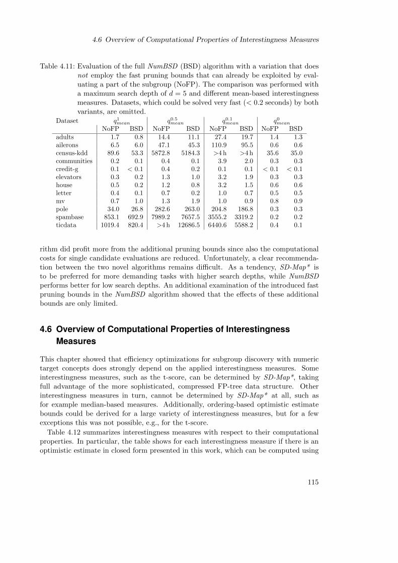
4.6 Overview of Computational Properties of Interestingness Measures
Table 4.11: Evaluation of the full NumBSD (BSD) algorithm with a variation that doesnot employ the fast pruning bounds that can already be exploited by eval-uating a part of the subgroup (NoFP). The comparison was performed witha maximum search depth of d = 5 and different mean-based interestingnessmeasures. Datasets, which could be solved very fast (< 0.2 seconds) by bothvariants, are omitted.
Dataset q1mean q0.5mean q0.1mean q0mean
NoFP BSD NoFP BSD NoFP BSD NoFP BSDadults 1.7 0.8 14.4 11.1 27.4 19.7 1.4 1.3ailerons 6.5 6.0 47.1 45.3 110.9 95.5 0.6 0.6census-kdd 89.6 53.3 5872.8 5184.3 >4 h >4 h 35.6 35.0communities 0.2 0.1 0.4 0.1 3.9 2.0 0.3 0.3credit-g 0.1 < 0.1 0.4 0.2 0.1 0.1 < 0.1 < 0.1elevators 0.3 0.2 1.3 1.0 3.2 1.9 0.3 0.3house 0.5 0.2 1.2 0.8 3.2 1.5 0.6 0.6letter 0.4 0.1 0.7 0.2 1.0 0.7 0.5 0.5mv 0.7 1.0 1.3 1.9 1.0 0.9 0.8 0.9pole 34.0 26.8 282.6 263.0 204.8 186.8 0.3 0.3spambase 853.1 692.9 7989.2 7657.5 3555.2 3319.2 0.2 0.2ticdata 1019.4 820.4 >4 h 12686.5 6440.6 5588.2 0.4 0.1
rithm did profit more from the additional pruning bounds since also the computationalcosts for single candidate evaluations are reduced. Unfortunately, a clear recommenda-tion between the two novel algorithms remains difficult. As a tendency, SD-Map* isto be preferred for more demanding tasks with higher search depths, while NumBSDperforms better for low search depths. An additional examination of the introduced fastpruning bounds in the NumBSD algorithm showed that the effects of these additionalbounds are only limited.
4.6 Overview of Computational Properties of InterestingnessMeasures
This chapter showed that efficiency optimizations for subgroup discovery with numerictarget concepts does strongly depend on the applied interestingness measures. Someinterestingness measures, such as the t-score, can be determined by SD-Map*, takingfull advantage of the more sophisticated, compressed FP-tree data structure. Otherinterestingness measures in turn, cannot be determined by SD-Map* at all, such asfor example median-based measures. Additionally, ordering-based optimistic estimatebounds could be derived for a large variety of interestingness measures, but for a fewexceptions this was not possible, e.g., for the t-score.
Table 4.12 summarizes interestingness measures with respect to their computationalproperties. In particular, the table shows for each interestingness measure if there is anoptimistic estimate in closed form presented in this work, which can be computed using
115

4 Algorithms for Numeric Target Concepts
FP-trees, if it is estimable by ordering, and if the measure itself is computable by theSD-Map* algorithm.
Table 4.12: A summary of interestingness measure with respect to properties regardingefficient computation.
Mea
sure
Not
ati
on
For
mu
la
Est
imate
incl
ose
dfo
rm
Est
imab
leby
ord
erin
g
Com
pu
tab
lein
SD
-Map*
Impact q1mean(P ) iP (µP − µ∅) yes one-pass yes
Generic mean qamean(P ) iPa(µP − µ∅) yes one-pass yes
z-score qz(P )√iP
(µP−µ∅)σ0
yes one-pass yes
Generic variance-based qaσ(P ) iPa(σP − σ∅) no no yes
t-score qt(P )√iP
(µP−µ∅)σs
no no yes
Generic symmetric mean qasym(P ) iPa|µP − µ∅| yes two-pass yes
Variance reduction qvr(P ) iP(i∅−iP )(µP − µ∅)2 yes two-pass yes
Generic median measure qamed(P ) iPa(meds −med0) (yes)2 one-pass no
Kolmogorov-Smirnov qks(P )√
iP ·|s|i∅
∆P,¬P yes no3 no
Mann-Whitney qmw(P )√
iP|s| (RiP− i∅
2 ) yes one-pass yes
Area-under-the-curve qauc(P )R− i¬P i¬P+1
2iP |s| yes one-pass yes
4.7 Summary
This chapter analyzed the task of efficient exhaustive subgroup discovery with numerictarget concepts. For this task, improvements were introduced in several directions: Noveloptimistic estimate bounds were proposed for a large variety of interestingness measures.While some of the bounds are expressed in closed forms based on few key statistics, oth-ers rely on a specific property of interestingness measures, which was introduced in thiswork. For the most popular class of measures in that area, generic mean-based mea-sures, additional bounds were proposed that can be applied with only partial knowledgeof the currently evaluated subgroup, allowing to prune a candidate pattern before its fullevaluation. Additionally, it was shown how popular data structures for subgroup dis-covery can be adapted to the task of subgroup discovery with numeric target concepts.
2The generic measure itself cannot be computed by SD-Map*.3Not yet determined.
116

4.8 Appendix
The proposed improvements are incorporated in two novel algorithms, that is, the SD-Map* algorithm and the NumBSD algorithm. An extensive runtime evaluation shows,both algorithms achieve runtime improvements of more than an order of magnitude incomparison to a basic approach.
4.8 Appendix
Lemma 1 Using the notations of Theorem 19, the function fa(x)(n+x)a ·(σ+x·θn+x − µ∅
)has no local maxima inside its domain of definition:
fa(x) ≤ max(f(0), f(xmax)) 2
Proof We distinguish three cases by the parameter a of the applied generic meaninterestingness measure:
First, for a = 1, it holds that
f1(x) = (n+ x)1 ·(σ + x · θn+ x
− µ∅)
= σ + θx− µ∅n− µ∅x= (θ − µ∅) · x+ σ − µ∅n
As this is a linear function in x, the function f1(x) is strictly increasing for θ > µ∅ andstrictly decreasing otherwise. Thus, the theorem holds for a = 1.
Second, we consider the case (a 6= 1)∧(σ = θn), that is, the first n instances all had thesame target value. In this case, the function fa(x) is given by fa(x) = (n+ x)a(θ− µ∅).This is strictly monotone since n > 0, x > 0. Thus, again f (x) has no local maximum.
Third, the case (a 6= 1)∧ (σ 6= θn) is considered in detail: Since σ was computed as asum of n values that are at least as large as θ it can be assumed that θ · n < σ. In thefollowing, the maxima of fa(x) is determined by deriving this function twice.
fa ′(x) =d
dxfa(x) = (n+ x)a ·
(σ + x · θn+ x
− µ∅)
= (n+ x)a(d
dx(θx+ σ
n+ x− µ∅)
)+
(θx+ σ
n+ x− µ∅
)·(d
dx(n+ x)a
)= (n+ x)a
(d
dx(θx+ σ
n+ x)
)+
(θx+ σ
n+ x− µ∅
)· a(n+ x)a−1
= (n+ x)a(
θ
n+ x− θx+ σ
(n+ x)2
)+
(θx+ σ
n+ x− µ∅
)· a(n+ x)a−1
= (n+ x)a−2 ((θ(n+ x)− (θx+ σ)) + a (θx+ σ − µ∅(n+ x)))
= (n+ x)a−2(θn− σ + aθx+ aσ − aµ∅n− aµ∅x))
= (n+ x)a−2 ((x(aθ − aµ∅) + aσ − aµ∅n+ θn− σ)
117

4 Algorithms for Numeric Target Concepts
In line 2, the product rule is used. In line 3 the chain rule is applied, substituting (n+x).µ∅ can be omitted, as it is constant with respect to x. In line 4 the quotient rule is used.Finally, in line 5 (n+ x)a−2 is factored out.
Since x > 0, n > 0 by definition, the first factor is obviously greater than zero for anyvalid x. For a = 0 or θ = µ∅, the second factor of this function is independent from x,so it has no root, thus f(x) has no maxima except the definition boundaries in this case.Otherwise the root of this function and therefore the only candidate for a maximum offa(x) is given at the point
x∗ =−aσ + anµ∅ − θn+ σ
a(θ − µ∅).
In the following, it is shown that x∗ can not be a maximum value in our setting: Forthat purpose, the second derivative of f(x) is computed at the point x∗:
fa ′′(x) =d
dxf ′(x)
= (n+ x)a−3(a− 2)(x(aθ − aµ∅) + aσ − an+ θn− σ) + (aθ − aµ∅)(n+ x)a−2
= (n+ x)a−3((a− 2)(x(aθ − aµ∅) + aσ − anµ∅ + θn− σ) + (aθ − aµ∅)(n+ x))
= (n+ x)a−3(a2xθ − a2xµ∅ + a2σ − a2µ∅n+ aθn− aσ − 2xaθ + 2axµ∅ − 2aσ
+ 2anµ∅ − 2θn+ 2σ + aθn− anµ∅ + aθx− axµ∅)= (n+ x)a−3(a− 1)(aθx+ aσ − anµ∅ − axµ∅ + 2θn− 2σ)
= (n+ x)a−3(a− 1)(x(aθ − aµ∅) + aσ − anµ∅ + 2θn− 2σ)
We now can determine the second derivative of f in x∗:
fa ′′(x∗) = (n+ x∗)a−3(a− 1)(x∗(aθ − aµ∅) + aσ − anµ∅ + 2θn− 2σ)
= (n+ x∗)a−3(a− 1)(−aσ + anµ∅ − θn+ σ
a(θ − µ∅)(aθ − aµ∅) + aσ − anµ∅ + 2θn− 2σ)
= (n+ x∗)a−3(a− 1)(−aσ + anµ∅ − θn+ σ + aσ − anµ∅ + 2θn− 2σ)
= (n+ x∗)a−3(a− 1)(θn− σ)
= (n+ x∗)a−3(a− 1)(θn− σ)
Since fa(x) is defined only for positive x, the first factor is always positive. Since bypremise a < 1 and θn < σ, the second derivative at point x∗ is always positive. Thus,if x∗ is an extreme value of f(x), then it is a local minimum. Since it was shown abovethat f(x) has no other candidates for extreme values besides x∗, this proves the lemma.�
118

5 Efficient Exhaustive Exceptional ModelMining through Generic Pattern Trees1
The next chapter approaches the task of efficient exhaustive exceptional model min-ing [170]. In this variation of subgroup discovery, not the deviation of a single tar-get attribute determines the interestingness value of a subgroup, but the deviation inthe model parameters of a model that is derived from a set of model attributes, seeSections 2.4.3 and Section 2.5.3.4. For this task, generic pattern trees (GP-trees) areintroduced. These are novel data structures that enable fast discovery algorithms.
Since for exceptional model mining the search space is identical to traditional subgroupdiscovery, enumeration orders can be directly transfered from this setting. Regardingpruning possibilities, upper bounds can be determined for specific interestingness mea-sures. As an example, an interestingness measure, which uses a correlation coefficientmodel, could exploit the fact that the correlation coefficient never exceeds a value of1. However, there is a wide variety of model classes and for each of these model classesdifferent interestingness measures are applied. Since optimistic estimates bounds have tobe determined separately for each interestingness measure, it is difficult to find genericimprovements, which are applicable in most settings.
Therefore, efficient and generic data structures for exhaustive mining of exceptionalmodels are the focus of this chapter in order to achieve runtime improvements for alarge number of models classes and interestingness measures. In particular, the well-known FP-tree [111] data structure is significantly extended by replacing the frequencyinformation stored in each node of the tree by the more general concept of valuationbases. Valuation bases are dependent on a specific model class and allow for efficientcomputation of the target model parameters. We call these generalized data structuresgeneric pattern trees. They are used to derive an efficient novel algorithm, which isflexible: While the main search algorithm and core data structure is the same for allmodel classes, small parts of the data structure, that is, the valuation bases, can beplugged-in to adapt the algorithm to new model classes.
The contribution of this chapter is fourfold: First, the concept of valuation bases ispresented. It allows for deriving a new algorithm, which is capable of performing efficientexhaustive mining for many different classes of exceptional models. Second, the scope ofthe presented approach is characterized by a theorem that determines, if GP-trees canbe used for a certain model class or not. Third, instantiations of GP-trees are discussed
1This chapter is based on previously published work [173]: Florian Lemmerich, Martin Becker, andMartin Atzmueller. Generic Pattern Trees for Exhaustive Exceptional Model Mining. In Pro-ceedings of the European Conference on Machine Learning and Knowledge Discovery in Databases(ECML/PKDD), 2012.
119

5 Efficient Exhaustive Exceptional Model Mining through Generic Pattern Trees
for several important model classes, which have been presented in literature. Fourth, thepresented approach is evaluated using publicly available UCI data [13]. In that direction,also a scalability study on a real world dataset is performed.
The chapter is organized as follows: After a short outline of related work in Section 5.1,the concept of valuation bases as well as the novel algorithm is presented in Section 5.2.Then, the limitations of the presented approach with respect to the applicability todifferent model classes is characterized in Section 5.3. Afterwards, Section 5.4 discussesinstantiations of the presented generic algorithm by showing how different model classespresented in literature fit in the proposed framework. The effectiveness of the approachis evaluated in Section 5.5. Finally, the main results of this chapter are summarized inSection 5.6.
5.1 Related Work
Since the concept of exceptional model mining has been introduced only recently, veryfew generic algorithms have been proposed for that task. In the original paper intro-ducing this concept, Leman et. al. propose to use a heuristic beam search strategyfor the mining process [170]. Additional constraints on the pattern complexity and theminimum support are used to speedup the search. Van Leeuwen and Knobbe extendedthis approach in the DSSD algorithm to achieve a more diverse and non-redundant setof result patterns [242, 243]. Another approach by van Leeuwen is the EMDM algo-rithm [241]. This method follows a two-step approach: In the first step (EM step) acandidate subgroup is refined to maximize its exceptionality. A second step (DM step)aims at minimizing the description complexity of the candidate pattern by utilizing over-fitting preventing mechanisms of a (rule-based) classifier. These steps are iterated untilno more changes occur. In contrast to these heuristic algorithms, the generic algorithmproposed in this work performs an exhaustive search over the search space and thusguarantees optimal results.
For multi-label subgroup discovery, Mueller et al. present a subgroup discovery algo-rithm in a case study on breast cancer diagnosis as an improvement of Apriori-SD [198].In addition to the original algorithm, their development SD4TS also utilizes pruning onsubgroup support and interestingness measure-based pruning on the multi-label inter-estingness measure they use.
Atzmueller and Mitzlaff proposed the COMODO algorithm for descriptive communitymining [19], which could be considered as a specific exceptional mining task. While thisalgorithm also features prefix trees as a data structures, it is only suited for a specificmodel class in this particular problem setting. In contrast, the approach presented hereprovides a generic algorithm which can be used for a wide range of model classes andinterestingness measures.
120

5.2 GP-growth
Subgroup Valuation Basis Model Parameters Interestingnessφ χ q
Figure 5.1: The pipeline visualizing the novel approach: For each subgroup (set of datainstances) a valuation basis is derived using a function φ (valuation projec-tor). The model parameters for the chosen model class is extracted fromthese valuation bases using another function χ (model extractor). Modelparameters are then used to determine the interestingness of the respectivepattern using an exceptionality measure q.
5.2 GP-growth
In this section, a new approach on exhaustive exceptional model mining is presented.The novel method is called generic pattern growth (GP-growth), cf. also [36]. GP-growth is based on the FP-growth algorithm substituting frequencies by an intermediate,condensed data representation called a valuation basis, which is introduced first. Then,the modifications of the traditional FP-growth algorithm that lead to the novel GP-growth algorithm are discussed.
5.2.1 The Concept of Valuation Bases
In the traditional FP-growth approach, frequencies are stored in the nodes of the tree,cf. Section 3.3.3. These nodes can then be aggregated to obtain frequencies for patterns(itemsets, subgroups) in the search space. The frequency is then used to rate the patternsdetermining those with high instance counts. In the proposed approach, this frequencycount, which is stored in each node of the tree structure, is replaced by a more genericconcept that we call a valuation basis.
A valuation basis is defined as a (condensed) representation of a set of data instancesthat is sufficient to extract the model parameters for a given model class. Consequently,the kind of information stored in a valuation basis is dependent on the model class. Sincethe interestingness of a subgroup in our setting is based on the model parameters only,it can be derived from such a valuation basis.
A visualization of the overall approach is given in Figure 5.1: For each subgroup (set ofdata instances) a valuation basis can be derived using a function φ (valuation projector),e.g., by aggregating information on subsets of the subgroup. The model parameters forthe chosen model class are extracted from these valuation bases using another functionχ (model extractor). Model parameters are then used to determine the interestingnessscore of the respective pattern using an exceptionality measure q.
The data structure for the SD-Map* algorithm from Chapter 4 can be seen as a simpleexample for this approach: Consider a model with a single model attribute X. The onlymodel parameter is the mean value of X in all instances covered by the subgroup. Then,an appropriate valuation base can consist of the instance count and the sum of all values
121

5 Efficient Exhaustive Exceptional Model Mining through Generic Pattern Trees
of X of all instances of the subgroup. The instance count and the sum of values canbe accumulated in an FP-tree like structure. Given the accumulated valuation basisfor each pattern, the stored instance count and the value sum are used to compute themean. The actual interestingness value of the pattern can then be determined using thismean value, e.g. as the deviation from the mean value in the total population.
Please note that one can construct a trivial type of valuation bases that defines avaluation basis as the exact same set of data instances it represents (restricted to themodel attribute values). That is, in each tree node a complete list with references to allinstances is stored. Obviously, this most general type of valuation bases trivially containsall relevant information associated with the original set of data instances. Therefore,model parameters for any model class on the original set of data instances can be derivedfrom this type of valuation bases. However, while this trivial kind of valuation basisallows for a generally applicable approach, the main advantages in terms of memory andruntime performance are lost. Therefore, one aims to construct valuation bases for agiven model class which are as small as possible. A valuation basis is called condensedvaluation basis if its memory requirement is sublinear with respect to the number ofinstances it represents. The examples of valuation bases, which are presented in thiswork, use constant memory with respect to the instance count.
The possibility of aggregating valuation bases corresponding to sets of data instancesis modeled by valuation domains:
Definition 4 (Valuation Domain, Valuation Basis) A valuation domain is an a-belian semi-group V = (V,⊕), where V is an arbitrary set and ⊕ is a binary operatoron V , i.e. ⊕ : V × V → V and
� V is closed under ⊕, i.e. a, b ∈ V ⇒ a⊕ b ∈ V
� ⊕ is associative, i.e. a, b, c ∈ V ⇒ a⊕ (b⊕ c) = (a⊕ b)⊕ c
� ⊕ is commutative, i.e. a, b ∈ V ⇒ a⊕ b = b⊕ a
An element v ∈ V is called a valuation basis. 2
In order to derive valuation bases from data instances, we define the notion of avaluation projector φ as in Definition 5.
Definition 5 (Valuation Projector) Let I be a set of all data instances and letV = (V,⊕) be a valuation domain. Then a valuation projector is defined as
φ : I → V 2
Given the definition of valuation domains above, the valuation projector φ can benaturally extended to sets of data instances S ∈ 2I :
φ : 2I → V
S 7→⊕s∈S
φ(s)
122

5.2 GP-growth
As a result, for any disjunct pair of sets of data instances S′ ∩ S′′ = ∅ it holds that:
φ(S′ ∪ S′′) = φ(S′)⊕ φ(S′′)
Sometimes subgroups are evaluated by comparing the values of the model attributesderived in the subgroup and the complement of the subgroup. In order to handle this caseefficiently, an additional subtraction operator is required for the valuation domain:Let I be the set of all instances and let I ′′ ∪ I ′′ be an arbitrary partition of I. If thevaluation basis of I ′ is subtracted from the valuation basis of I, then the result mustbe the valuation basis of I ′′: φ(I) φ(I ′) = φ(I ′′). Thus, the valuation basis for thecomplement can easily be derived by subtracting the subgroup’s valuation basis fromthe overall valuation basis. The overall valuation basis can easily be computed in aninitial pass over the dataset.
5.2.2 Algorithmic Adaptations
Essentially, the FP-growth algorithm (cf. Section 3.3.3 for a detailed description) isgeneralized by substituting frequencies with the more general concept of valuation bases.The resulting algorithm is called GP-growth. The generalized tree structure that storesvaluation bases instead of frequencies is called a GP-tree.
Whereas the FP-growth algorithm adds up frequencies in its FP-trees, the GP-growthalgorithm aggregates valuation bases in its GP-trees. Hence, GP-growth produces aggre-gated valuation bases instead of frequencies for each pattern. Note that a valuation basiscan also contain a frequency as described in the mean value example in Section 5.2.1.An illustration of this approach is given in Figure 5.2.
In order to aggregate valuation bases for each pattern, the algorithm requires
� a valuation domain V = (V,⊕) to draw valuation bases from,
� a valuation projector φ to project single data instances onto valuation bases, and
� optionally a subtraction operator to support complement comparisons as men-tioned in Section 5.2.1 if the statistics for the complement are required by theutilized exceptionality measure.
Patterns are then evaluated based on their valuation bases by applying
� a model extractor χ to map valuation bases v ∈ V onto model parameters, and
� an exceptionality measure q based on these model parameters.
These adaptations of FP-growth allow for a generic implementation. That is, the codefor the main algorithm is identical for all model classes. To apply it to a new modelclass, only the valuation domain with its aggregation operator ⊕, the correspondingvaluation projector φ, and the model extractor χ must be implemented. We call thetuple (V,⊕, φ, χ) a model configuration.
123

5 Efficient Exhaustive Exceptional Model Mining through Generic Pattern Trees
∅count: 18
acount: 10
bcount: 3
bcount: 5
. . .
(a) Exemplary tree structure of a traditional FP-tree
∅VB
b
VB
a
VB
b
VB
. . .
count: 3sum(X): 5
sum(X2): 18
Variance model class
count: 3sum(X): 5
sum(Y ) = 8C = 18
sum(X2): 113sum(Y 2) = 30
Correlation coefficientmodel class
. . .
(b) Exemplary tree structure of a GP-tree, the novel data structure introduced in this work
Figure 5.2: An example for the generalization from FP-trees to GP-trees: The tree struc-ture and the auxiliary links that connect nodes for same selector remainsidentical, but the information stored in each node differs. In traditionalFP-trees only the count for the corresponding set of instances is saved. Incontrast, in GP-trees the nodes store valuation bases, which contain moreinformation. The kind of information that is saved in the valuation basesdepends on the chosen model class of the mining task. Thus, the main datastructure is the same for all model classes, but the valuation bases can beexchanged in order to adapt to novel model classes.
124

5.3 Theorem on Condensed Valuation Bases
Please note, that for the very simple valuation basis, which only counts the instances,the resulting algorithm is identical to FP-growth. Furthermore, traditional subgroupdiscovery can be implemented in this generic algorithm by using valuation bases thatcount instances with a positive and a negative target concept separately, as done in theSD-Map algorithm [22]. Thus, the approach presented in this work can be regarded as atrue generalization of both, FP-growth [111] and SD-Map. The SD-Map* algorithm islimited to the setting with a single numeric target variable, but does additionally provideefficient, specialized pruning options. In the future, pruning could also be incorporatedin the GP-growth algorithms, if the respective optimistic estimate bound are derived forthe utilized interestingness measures. Unfortunately, these have not yet been researchedfor exceptional model mining.
5.3 Theorem on Condensed Valuation Bases
The approach of generalized FP-trees is especially efficient if it is possible to derive asmall condensed valuation basis for a model class. If the constructed model itself is verycomplex, then it seems difficult to derive suitable condensed valuation bases that aresufficient to extract the model parameters. This includes, for example, computationallyexpensive models that involve the learning of a bayesian network as explored in [73].
In order to define the scope of the presented approach, the following theorem charac-terizes model classes, for which GP-trees can be applied with strongly reduced memoryrequirements. This is done by drawing a parallel to data stream mining:
Theorem 1 There is a condensed valuation domain for a given model class if and onlyif the following conditions are met: (1) There is a parallel single-pass algorithm withsublinear memory requirements to compute the model parameters from a given set ofinstances, which are distributed randomly on one of the (parallel) computation nodes;(2) the only communication between the computation nodes in this algorithm takes placewhen combining results. 2
Proof ⇒: First, assume there is a model configuration (V,⊕, φ, χ) that can be used todetermine the model parameters of a subgroup. Then, a parallel single-pass algorithmcan be constructed as following: In each computation node N one loops through allinstances IN assigned to this node, updating the respective valuation basis vN . For eachinstance c ∈ IN , the valuation basis φ(c) is extracted and used to update the currentaccumulated valuation basis: vnewN = voldN ⊕φ(c). Thus, after each step the valuation basisvN corresponds to all instance handled so far. After the loop through all instances of thiscomputation node, the valuation basis vN can be used to extract the model parametersfor the set of instances IN . Furthermore, the resulting valuation bases from differentcomputation nodes can be combined by using the aggregation operator ⊕ again. Thisleads to a valuation basis that corresponds to all instances of the dataset. The modelparameters are then extracted using the model extractor χ; this completes the parallelsingle-pass algorithm for computing these parameters.
125

5 Efficient Exhaustive Exceptional Model Mining through Generic Pattern Trees
⇐: Assume there is a parallel single-pass algorithm with the properties presentedabove. Then, there is a set of variables VC that are used in the computation within eachof the nodes, which is sublinear with respect to the number of contained instances. Itis shown that this set of variables defines a model configuration (V,⊕, φ, χ). Since thealgorithm is single-pass, the assignments for these variables are updated only once foreach instance using the values of the model attributes for this instance. Now let vi bethe vector of values (variable assignments) of the variables VC after the instance i isprocessed as the first instance in this computation node. Then, one can use this vectoras the projector function φ(i) = vi. This is sufficient for a valuation basis; if there wasonly one instance in the dataset, then a correct algorithm would be able to extract themodel parameters for the model built from the single instance using only the data vi.
Next, assume that each computational node Nj has finished the computation of itspartition of the data Dj , each resulting in variable assignments vj , which correspondto a valuation basis. vj must be sufficient to extract the model parameters for thedata Dj since Nj could be the only computational node. The method used for thissubtask can be regarded as a model extractor function χ. Now consider two valuationbases v1 and v2 that result from two computation nodes and are corresponding to datapartitions D1 and D2. A correct parallel algorithm must come with an appropriatemethod to combine the results v1 and v2 into new variable assignments that is suited toextract model parameters for the data D1 ∪D2. This method can be used as a generalaggregation function ⊕ for valuation bases. Thus, given a parallel single-pass algorithmwith the properties presented above one can derive a model configuration (V,⊕, φ, χ).�
The proof is constructive. It describes a method to transfer parallel single-pass algo-rithms for specific model classes to valuation domains that can be used for efficientexceptional model mining with GP-trees. Some important examples of this approachare shown in the next section.
5.4 Valuation Bases for Important Model Classes
This section discusses the application of GP-trees to different model classes. Most of thepresented model classes have been proposed in [170], to which it is referred for a moredetailed description of the models and exceptionality measures.
5.4.1 Variance Model
The variance model identifies patterns, in which the variance of a single target variableX is especially high/low. Although this model features only a single model attribute,this task can not be accomplished by traditional subgroup discovery algorithms utilizingFP-trees, such as SD-Map.
For an efficient computation of the variance, the following well known formula isutilized:
V ar(X) = E[X2]− E[X]2 =
∑x2
n− (
∑x
n)2,
126

5.4 Valuation Bases for Important Model Classes
where E[X] is the expected value for the variable X. For computing the variance of anattribute, only the total count, the sum of all values and the sum of all squared values arerequired. Formally, a model configuration (Vσ,⊕σ, φσ, χσ) that is sufficient to computethe variance (or equivalently, the standard deviation) of a variable X can be defined as:
Vσ = R3
v ⊕σ u = v + u
φσ(c) = (1, X(c), X(c)2)T
χσ(v) =v3
v1− (
v2
v1)2
Each valuation basis stores a vector of three real numbers. Aggregating valuationbases using the operator ⊕ is equivalent to adding vectors in euclidean space. Thevaluation basis extracted from a single data instance c contains the constant 1 as theinstance count, the value of X in c and the squared value of X in c. To extract themodel parameter V ar(X) from a valuation basis v ∈ Vσ, the computation χσ has to beperformed using the three components of the vector stored in the valuation basis v.
Example 13 Assume that in the mining algorithm a new tree node is created for aninstance i1, where the single model attribute X takes the value X(i1) = 5. Like any treenode in this settings, the new node stores three values, in this case 1, 5, and 52 = 25.Now assume another node v in the tree structure corresponds to three instances withvalues X(i2) = 2, X(i3) = 3, and X(i4) = 10. Thus, the values in v are 3, 15, and113. In the mining algorithm tree nodes are aggregated to create new nodes, whichthen correspond to the union of instances of the single nodes. Assume that both nodesdescribed above are aggregated. Then the values stored in the novel node are determinedas: (1, 5, 25)T + (3, 15, 113)T = (4, 20, 138)T . The variance for the four instances, whichcorrespond to this new node can be computed as: 138
4 − (204 )2 = 34.5− 25 = 9.5. 2
5.4.2 Correlation Model
The (Pearson product-moment) correlation coefficient ρ(X,Y ) is a very well known sta-tistical measure that reflects the linear dependency between two numerical attributes Xand Y . The correlation coefficient is defined as the fraction of the covariance and theproduct of the standard deviations of these two attributes: ρ(X,Y ) = Cov(X,Y )
σXσY.
We will first derive a model configuration for the covariance. This will then be utilizedto derive a configuration for the correlation model. The covariance of a set of instances
is defined as CovS(X,Y ) =∑
(x,y)(x−µX)(y−µY )
N , where µX (µY ) describes the mean valueof the attribute X (Y ) in the instance set S and N the number of instances in S. In thevaluation domain for GP-trees, which is derived here, the measures Cov(X,Y ), σX andσY are determined independently from each other.
127

5 Efficient Exhaustive Exceptional Model Mining through Generic Pattern Trees
To efficiently compute the covariance of two variables X,Y a pairwise update for-mula was introduced in [38] for a parallel single-pass algorithm. It allows to computeCS(X,Y ) = CovS(X,Y ) · |S| =
∑(x,y)∈S(x − µX)(y − µY ) for a set of data instances
S = S1 ∪S2, S1 ∩S2 = ∅ given statistical information of the partitioning sets S1 and S2:
CS(X,Y ) = CS1(X,Y ) + CS2(X,Y ) +iS1iS2
iS1 + iS2
(µX,2 − µX,1)(µY,2 − µY,1),
where iS1 = |S1| and iS2 = |S2| denote the instance count in S1 and S2, and µX,2,µX,1, µY,2, µY,1 are the mean values of X and Y in the sets S1 and S2. According toTheorem 1, this update formula can be used to construct a model configuration for thecorrelation model.
To compute the covariance for each subgroup with this formula, one needs to keeptrack of the value of CS(X,Y ) in the respective set of instances, the cardinality (numberof instances) of the subgroup, and the mean values of the variables X and Y . Thelatter can be computed by the sum of the values for the respective attributes and thecardinality of the subgroup. Therefore, a model configuration for the covariance can bedefined by using the above formula:
Vcov = R4
v ⊕cov u =
v1
v2
v3
v4
⊕u1
u2
u3
u4
=
v1 + u1
v2 + u2
v3 + u3
v4 + u4 + v1u1v1+u1
(v2v1− u2
u1)(v3v1− u3
u1)
φcov(c) = (1, X(c), Y (c), 0)T
χcov(v) =v4
v1
In this formalization of a model configuration, the first component of a valuation basisreflects the size of the corresponding set, the second and third component store the sumof the values of X and Y and the fourth component keeps track of the measure C asdefined above.
To compute the actual correlation coefficient this valuation basis is combined with thevaluation basis used for the variance model in order to compute Cov(X,Y ), σX and σYin a single model configuration:
128

5.4 Valuation Bases for Important Model Classes
Vcor = R6
v ⊕cor u =
v1
v2
v3
v4
v5
v6
⊕
u1
u2
u3
u4
u5
u6
=
v1 + u1
v2 + u2
v3 + u3
v4 + u4 + v1u1v1+u1
(v2v1− u2
u1)(v3v1− u3
u1)
v5 + u5
v6 + u6
φcor(c) = (1, X(c), Y (c), 0, X(c)2, Y (c)2)T
χcor(v) =Cov(X,Y )
σXσY=
v4v1√
v5v1− (v2
v1)2√
v6v1− (v3
v1)2
=v1v4√
v1v5 − v22
√v1v6 − v2
3
Example 14 Consider model attributes X and Y and the small dataset shown in Ta-ble 5.1: When mining for exceptional correlation models, each tree node in the generic
Table 5.1: A small example dataset with values for the model attributes X and Y .
instance X Y
i1 5 3i2 2 1i3 3 2i4 10 5
pattern tree stores six values. When a new tree node u is created for i1, it storesthe values using the function φcor(c): 1, X(i1) = 5, Y (i1) = 3, 0, X(i1)2 = 25, andY (i1)2 = 9. Another node v in the tree structure corresponds to three instances i2, i3, i4.To compute the respective stored values is slightly more complicated, they turn out tobe (3, 15, 8, 18, 113, 30)T in vector notation. Assume that both nodes described aboveare aggregated to create a new node, which then correspond to the union of instancesof the respective single nodes, that is, i1, i2, i3, and i4. Then the six values stored in thenovel node are determined by the aggregation operation ⊕cor: 1 + 3 = 4, 5 + 15 = 20,3 + 8 = 11, 0 + 18 + 1·3
1+3(51 −
153 )(3
1 −73) = 18, 25 + 113 = 138, and 9 + 30 = 39. The
correlation coefficient for these four instances is then computed based on the informationstored in the node with the function χcor:
4·18√4·138−202
√4·39−112
≈ 0.987. 2
129
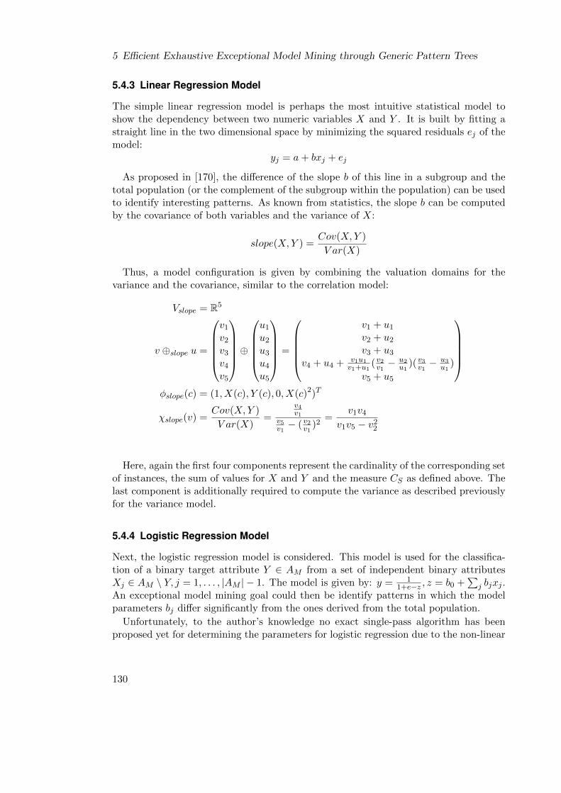
5 Efficient Exhaustive Exceptional Model Mining through Generic Pattern Trees
5.4.3 Linear Regression Model
The simple linear regression model is perhaps the most intuitive statistical model toshow the dependency between two numeric variables X and Y . It is built by fitting astraight line in the two dimensional space by minimizing the squared residuals ej of themodel:
yj = a+ bxj + ej
As proposed in [170], the difference of the slope b of this line in a subgroup and thetotal population (or the complement of the subgroup within the population) can be usedto identify interesting patterns. As known from statistics, the slope b can be computedby the covariance of both variables and the variance of X:
slope(X,Y ) =Cov(X,Y )
V ar(X)
Thus, a model configuration is given by combining the valuation domains for thevariance and the covariance, similar to the correlation model:
Vslope = R5
v ⊕slope u =
v1
v2
v3
v4
v5
⊕u1
u2
u3
u4
u5
=
v1 + u1
v2 + u2
v3 + u3
v4 + u4 + v1u1v1+u1
(v2v1− u2
u1)(v3v1− u3
u1)
v5 + u5
φslope(c) = (1, X(c), Y (c), 0, X(c)2)T
χslope(v) =Cov(X,Y )
V ar(X)=
v4v1
v5v1− (v2
v1)2
=v1v4
v1v5 − v22
Here, again the first four components represent the cardinality of the corresponding setof instances, the sum of values for X and Y and the measure CS as defined above. Thelast component is additionally required to compute the variance as described previouslyfor the variance model.
5.4.4 Logistic Regression Model
Next, the logistic regression model is considered. This model is used for the classifica-tion of a binary target attribute Y ∈ AM from a set of independent binary attributesXj ∈ AM \ Y, j = 1, . . . , |AM | − 1. The model is given by: y = 1
1+e−z , z = b0 +∑
j bjxj .An exceptional model mining goal could then be identify patterns in which the modelparameters bj differ significantly from the ones derived from the total population.
Unfortunately, to the author’s knowledge no exact single-pass algorithm has beenproposed yet for determining the parameters for logistic regression due to the non-linear
130

5.4 Valuation Bases for Important Model Classes
nature of parameter fitting. Since according to Theorem 1 the existence of such analgorithm is necessary for the existence of a sufficient condensed valuation basis, theefficient computation of parameters is not possible so far.
5.4.5 DTM-Classifier
The next discussed model is based on the DTM-classifier [152]: This method predictsa target attribute Y ∈ AM from a set of independent attributes Xj ∈ AM \ Y, j =1, . . . , |AM | − 1 by determining the probability of each target attribute value for eachcombination of values of the independent attributes. For value combinations, which didnot occur in the training set, the probability distribution of the complete training setis used. Then, for a given new instance i the target value is predicted that has thehighest probability conditioned on the respective combination of values of the Xj in i. Ifthe specific combination of the values of Xj did not occur in the training data, then theinstance is classified as the most frequent target value in the complete training set. In thecontext of exceptional model mining, amongst others, the Hellinger distance has beenproposed as an exceptionality measure for this model class. It measures the differencebetween the distribution within a subgroup P and the distribution in its complement¬P . It is computed as∑
y,x1,...xk
(√PP (y|x1, . . . , xk)−
√P¬P (y|x1, . . . , xk)
)2
For an efficient computation in FP-trees, the probabilities for all value combinationsof Y,X1, . . . , X|AM−1| are stored in the valuation basis.
In the following, all attributes are assumed to be binary for the sake of simpler no-tation. The generalization for non-binary attributes is straightforward. Furthermore,it is assumed that the combinations of values in the decision table are arranged in apredefined order, such that the positive values of Y are on odd positions and the corre-sponding negative value of Y for the same combination of independent attribute valuesis immediately following. Then, a slightly simplified model configuration is given by:
Vdtm = R2|AM |
v ⊕dtm u = v + u
φdtm(c) = (vj) =
{1, if the j-th combination of values is true in c0, else
χ(k)dtm(v) =
v2k−1
v2k−1 + v2k
In this model configuration, an index position is computed for each combination ofvalues. The valuation basis then stores the frequency counts for these combination ofvalues using these indices. Please note that in this case the valuation basis stored ineach node of the GP-tree needs to store 2m values, where m is the number of (binary)
131

5 Efficient Exhaustive Exceptional Model Mining through Generic Pattern Trees
model attributes. Therefore this model configuration is not tractable for large numbersof model attributes. However, this should not be the case in most practical applicationssince larger models are typically difficult to comprehend by human users.
5.4.6 Accuracy of Classifiers
One application of exceptional model mining could be, to identify subgroups, in which theclassification model learned from the instances of a subgroup is especially accurate/in-accurate for these instances. Assuming that the decision of the classifier is based on alllearning instances, the generalized FP-tree approach is not applicable for this task:
The computation of the accuracy of a classifier requires two passes through thedatabase. The first pass is used to determine the model parameters for the classifier.Then, a second pass over the instances is required to classify the instances. Accordingto Theorem 1, it is therefore not possible to construct a suitable condensed valuationbasis.
Please note that as a consequence the presented approach allows to efficiently findpatterns, in which the classification model built from the instances of this pattern differsstrongly from the model built from the entire population, but it is not possible to identifypatterns, in which this model performs exceptionally well or bad.
5.4.7 Bayesian Networks
Bayesian networks have been proposed as complex target models for exceptional modelmining [73]. Since to the best of the author’s knowledge there is currently no parallelsingle-pass algorithm for learning bayesian networks – which is a complex task on its own– a condensed valuation basis for this model class cannot be provided here. However,there is ongoing research in that area [50], which can possibly be exploited in futurework.
5.5 Evaluation
This section presents runtime evaluations of the proposed approach using publicly avail-able UCI-datasets [13] as well as a scalability study in a large real world dataset.
5.5.1 Runtime Evaluations on UCI data
The GP-tree approach was evaluated by performing runtime experiments using publiclyavailable UCI datasets. The algorithms were implemented in the subgroup discoveryenvironment VIKAMINE 2, see Chapter 8. The experiments were performed on a stan-dard office PC with a 2.2 GHz CPU and 2 GB RAM. The search space consisted ofthe non-model attributes in the respective dataset. For nominal attributes, attribute-value pairs were used as selectors. Numeric attributes were discretized into five intervalsby using equal-frequency discretization. Only intervals between two adjacent cutpointswere used as selectors.
132

5.5 Evaluation
Table 5.2: Runtime in seconds for the GP-growth algorithm using the credit-g datasetfor different model classes and various search depth (maximum number ofselectors in a single subgroup description).
Model Class 2 3 4 5
Frequent Itemsets 0.7 3.7 17.5 70.0Subgroup Discovery 0.7 3.6 17.3 68.2Variance 0.8 3.7 17.4 70.7Correlation Coefficient 0.8 4.0 19.2 77.3Linear Regression 0.8 4.0 19.1 78.2DTM-classifier 1.6 8.4 44.0 187.4
Table 5.3: Runtime in seconds for the GP-growth algorithm using the adults datasetfor different model classes and various search depth (maximum number ofselectors in a single subgroup description).
Model Class 2 3 4 5
Frequent Itemsets 4.7 8.5 19.8 50.4Subgroup Discovery 4.7 8.4 19.6 48.7Variance 4.7 8.5 19.8 50.1Linear Regression 4.8 8.9 21.8 55.8Correlation Coefficient 4.8 8.9 21.7 55.7DTM-classifier 15.1 36.7 90.2 213.7
Table 5.4: Runtime in seconds for the GP-growth algorithm using the autos datasetfor different model classes and various search depth (maximum number ofselectors in a single subgroup description).
Model Class 2 3 4 5
Frequent Itemsets 0.4 3.0 17.1 73.4Subgroup Discovery 0.4 2.9 16.3 72.3Variance 0.4 3.0 17.0 74.2Linear Regression 0.4 3.2 18.1 84.3Correlation Coefficient 0.4 3.2 18.0 81.1DTM-classifier 0.7 5.2 31.8 150.7
133

5 Efficient Exhaustive Exceptional Model Mining through Generic Pattern Trees
Table 5.5: Runtime in seconds for different UCI-Datasets for the linear regression modelclass for various search depth (maximum number of selectors in a single sub-group description), comparing a simple depth-first-search (DFS) with the GP-growth algorithm (GPG).
Max depth 2 3 4 5Dataset DFS GPG DFS GPG DFS GPG DFS GPG
adults 218.3 4.8 5481.2 8.9 >2 h 21.8 >2 h 55.8autos 1.4 0.4 42.7 3.2 632.8 18.1 5416.9 84.3breast-w 0.1 0.0 0.9 0.0 3.0 0.1 6.6 0.1census-kdd >2 h 227.0 >2 h 1139.9 >2 h 7418.9 >2 h >2 hcolic 1.4 0.8 33.5 2.3 428.5 10.9 3009.8 39.2credit-a 1.2 0.2 16.3 0.8 129.4 2.8 654.5 8.2credit-g 3.3 0.8 73.2 4.0 975.6 19.1 >2 h 78.6diabetes 0.3 0.1 2.2 0.1 10.2 0.2 28.4 0.3forestfires 0.8 0.1 11.8 0.5 93.3 1.6 378.6 3.6glass 0.1 0.0 0.8 0.1 3.6 0.1 8.6 0.2heart-h 0.2 0.1 2.1 0.1 10.9 0.3 34.1 0.5hepatitis 0.2 0.1 3.6 0.6 35.4 2.8 219.5 10.2hypothyroid 11.4 1.3 261.7 4.6 3791.7 21.8 >2 h 111.0ionosphere 3.1 1.5 145.1 18.9 3625.0 162.9 >2 h 1083.2labor 0.1 0.0 0.7 0.1 3.6 0.2 10.7 0.5segment 6.6 0.9 156.7 3.5 2153.9 15.3 >2 h 58.2spambase 19.3 4.3 627.7 20.9 >2 h 146.0 >2 h 1438.9vehicle 2.4 0.5 57.4 2.5 784.3 12.1 5956.8 43.1vowel 2.0 0.3 37.6 1.0 374.8 3.5 1808.0 8.5
In a first set of experiments the runtime of the GP-tree approach was comparedfor different model classes. For better comparability the two numeric attributes perdataset, which were used as model attributes for the correlation coefficient and the linearregression models, were also excluded from the search space for the frequent itemsets,subgroup discovery and variance model classes. In doing so, the search spaces for thesetasks were identical. Exemplary results for the datasets credit-g, adults and autos areshown in Tables 5.2, 5.3 and 5.4. Further experiments on other datasets showed thesame overall characteristics.
As can be seen in these tables, the algorithm runtimes for different model differ onlylittle. The runtimes for the model classes linear regression and correlation coefficient,which require slightly larger valuation bases, are increased marginally in comparison tothe simpler model class, e.g., the frequent itemset model. For the DTM-classifier, theresults only differ in our implementation by a small constant factor (about 2-4), whichcan explained by the required more complex model configuration. The similarity of theruntimes is due to the fact that no pruning scheme is utilized. Consequently, the search
134

5.5 Evaluation
Table 5.6: Runtime in seconds for different UCI-Datasets for the correlation coefficientmodel class for various search depth (maximum number of selectors in a singlesubgroup description), comparing a simple depth-first-search (DFS) with theGP-growth algorithm (GPG).
Max depth 2 3 4 5Dataset DFS GPG DFS GPG DFS GPG DFS GPG
adults 173.0 4.8 4794.9 8.9 0.0 21.7 >2 h 55.7autos 1.2 0.4 37.9 3.2 590.7 18.0 5125.4 81.1breast-w 0.1 0.0 0.7 0.0 2.5 0.1 5.7 0.1census-kdd >2 h 226.4 >2 h 1144.4 >2 h 7409.6 >2 h >2 hcolic 1.1 0.7 25.2 2.2 335.7 10.8 2419.0 38.0credit-a 0.9 0.2 13.0 0.8 106.0 2.8 553.7 8.2credit-g 2.5 0.8 58.1 4.0 814.3 19.2 6975.3 77.3diabetes 0.2 0.0 1.7 0.1 8.8 0.2 25.2 0.3forestfires 0.6 0.1 9.8 0.5 82.4 1.6 345.1 3.6glass 0.1 0.0 0.7 0.1 3.2 0.1 7.9 0.2heart-h 0.2 0.1 1.6 0.1 8.6 0.3 27.9 0.5hepatitis 0.2 0.1 2.7 0.6 27.8 2.8 177.9 10.3hypothyroid 8.4 1.3 200.3 4.6 3002.9 21.1 >2 h 108.5ionosphere 2.5 1.6 121.3 20.0 3272.3 161.1 >2 h 1053.0labor 0.1 0.0 0.6 0.1 2.8 0.2 8.3 0.5segment 5.2 0.9 129.3 3.5 1878.3 15.4 >2 h 58.9spambase 14.2 4.3 473.0 20.8 < 2h 148.0 >2 h 1459.4vehicle 1.8 0.5 46.8 2.6 680.1 12.3 5324.8 43.2vowel 1.6 0.3 32.2 1.0 343.4 3.5 1716.6 8.4
space is the same for all model classes and also the number of tree nodes and number ofrequired aggregations of tree nodes is identical.
Next, an extensive runtime analysis of our approach was performed using 19 datasetsfrom the UCI repository. For that purpose, the proposed GP-growth algorithm wascompared to a simple depth-first-search without any specialized data structure. Due tothe runtime similarity for different model classes, the presented results are limited to twoexemplary model classes, that is, the slope of the linear regression and the correlationcoefficient. The results are shown in Tables 5.5 and 5.6.
It can be observed that even at a search depth of 2 (searching only for subgroupdescriptions that have a maximum of 2 selectors) the GP-growth algorithm outperformsthe simple depth-first-search approach significantly. This difference increases for largersearch depth. At a search depth of 5, GP-growth completes the task more than an orderof magnitude faster for all datasets. These results clearly demonstrate the power ofefficient data structures such as the GP-tree.
135

5 Efficient Exhaustive Exceptional Model Mining through Generic Pattern Trees
5.5.2 Scalability Study: Social Image Data
In the following, a short case study on real world data is presented that demonstratesthe advantages of the presented approach in large scale applications. As a dataset,publicly available metadata of pictures uploaded to the Flickr2-platform was used. Morespecifically, the view counts as well as all tagging information were crawled of all pictureswhich are geo-referenced to a location in Germany and were uploaded in 2010. Details onthis dataset are provided in Section 9.2. The dataset was limited to tags with more than1000 occurrences. This lead to about 1200 tags that were used as describing attributesfor about 1.1 million instances.
Since pictures viewed by more people are naturally also tagged by more people, thereis a correlation to the number of tags assigned to a picture. To evaluate the scalabilityof the GP-growth approach, an exceptional model mining task was executed to identifycombinations of tags (as subgroup descriptions), for which this correlation is especiallystrong. As a result, even for a search depth of 2, the simple DFS algorithm did notfinish the task within two full days. In contrast, the same task performed by GP-growthfinished in about 8 minutes.
The massive difference for this dataset can be explained by the sparseness of thetagging data, which especially favors the utilized tree structure. Furthermore, even foran increased search depth of 3, the task could be completed within 10 minutes. Thissmall difference in comparison to a search depth of 2 is reasonable, as less combinationsof three tags occur in dataset than combinations of two tags due to the sparseness of thedataset. Overall, the runtime improvements for the Flickr dataset are even larger thanin the previously investigated smaller datasets, showing the scalability of our approach.
5.6 Summary
This chapter proposed a novel approach for fast exhaustive exceptional model mining:It introduced the concept of valuation bases as an intermediate condensed data repre-sentation and presented the generic GP-growth algorithm. This algorithm transfers theFP-tree data structure to the setting of exceptional model mining in order to allow forefficient exhaustive mining for a wide variety of model classes. The applicability of theproposed approach was discussed in detail: Model classes, for which the algorithm isapplicable, can be identified by a theorem that draws an analogy to data stream mining.For several model classes the implementations of the generic approach have been pre-sented. Runtime experiments show improvements of more than an order of magnitudeof the novel approach in comparison to a naive exhaustive depth-first-search.
2www.flickr.com
136

6 Difference-based Estimates forGeneralization-Aware Subgroup Discovery1
The next chapter introduces a novel approach to derive optimistic estimates for generali-zation-aware interestingness measures. In contrast to previous approaches the boundsare not only based on the anti-monotonicity of instances that are contained within thesubgroup. Instead, also the number of instances that are covered by a pattern, butnot by its generalizations are considered. This allows for significantly tighter optimisticestimate bounds and thus faster subgroup discovery when using generalization-awaremeasures.
For motivation, the problem setting is recapitulated in short, for more details see Sec-tion 2.5.4: The selection of subgroups is commonly based on an interestingness measure.These measures use statistics derived from the instances covered by a subgroup to deter-mine its score. The best subgroups according to this score are then returned to the user.As an example, consider a dataset of patients and their medical data. Let the targetconcept be surgery successful, which is true for 30% of the patients. Then a subgrouplike gender=male ∧ smoker=false with a higher rate of successful surgeries, e.g. 50%,receives a high score and is likely to be included in the result.
Practical applications have shown that results for traditional interestingness measuresoften contain variants of the same pattern multiple times. To avoid this problem, severalauthors postulated that a subgroup should not only be evaluated with respect to its ownstatistics, but also with respect to the statistics of its generalizations, see for instance [34,27, 29], see also Chapter 7. Considering the example above, the subgroup gender=male∧ smoker=false would be rated as less interesting if it can be explained by one ofits generalizations alone, e.g., if the subgroup smoker=false already describes a set ofpatients with a 50% surgery success rate. While the practical use of such generalization-aware interestingness measures has been widely acknowledged, the efficient mining inthis setting has received little attention.
A key technique to improve runtime performance of subgroup discovery in generalis the application of optimistic estimates, that is, upper bounds for the interestingnessof any specialization of the currently evaluated subgroup, cf. Section 3.4.2. Althoughresearch has shown that improving the tightness of the utilized bounds improves theruntime performance substantially [108], there has been no extensive research so far
1This chapter is based on previously published work [174]: Florian Lemmerich, Martin Becker, andFrank Puppe: Difference-Based Estimates for Generalization-Aware Subgroup Discovery. In Pro-ceedings of the European Conference on Machine Learning and Knowledge Discovery in Databases(ECML/PKDD), Best Paper Award, 2013.
137

6 Difference-based Estimates for Generalization-Aware Subgroup Discovery
concerning upper bounds for generalization aware interestingness measures beyond thetrivial transfer of bounds for traditional measures.
In this chapter, a novel method to exploit specific properties of generalization-awaremeasures to derive additional optimistic estimate bounds is proposed. Unlike previousapproaches, the bounds are not exclusively based on the instances that are contained inthe currently examined subgroup, but on the instances that were excluded in comparisonto generalizations of the current pattern. In doing so, tighter optimistic estimate boundscan be computed and the runtime of algorithms is significantly reduced. It is shown howthis general concept can be applied to exemplary interestingness measures in differentsetting, i.e., for subgroup discovery with binary target concepts and with numeric targetconcepts using a mean-based interestingness measure. The bounds are incorporated in anovel apriori -based algorithm that allows efficient propagation of the required statistics.The effectiveness of the presented approach is evaluated in experiments on publiclyavailable data. It can be observed that the novel optimistic estimates are especiallyeffective in tasks that incorporate selectors, which cover a majority of the dataset.
The rest of this chapter is structured as follows: Related work is discussed in Sec-tion 6.1. Next, the new scheme to derive optimistic estimate bounds and its applica-tion to different interestingness measures is presented in Section 6.2. Afterwards, it isexplained how the new optimistic estimate bounds can efficiently be exploited in an al-gorithm in Section 6.3. Section 6.4 presents experimental results, before main results ofthe chapter are summarized in Section 6.5.
6.1 Related Work
Pruning based on optimistic estimates [248, 260] is an essential technique for efficientsubgroup discovery. As Grosskreutz et al. showed, the efficiency of the pruning isstrongly influenced by the tightness of the bounds [108]. A more general method toderive optimistic estimates for a whole class of interestingness measures, that is, convexmeasures, was introduced in [196] and later extended in [274]. This chapter presents adifferent technique to determine optimistic estimates to another family of interestingnessmeasures, i.e., generalization-aware measures. In contrast to previous approaches, theoptimistic estimate of a subgroup is not exclusively based on the instances covered bythis subgroup, but takes also other, more general subgroups into account.
The necessity to consider also generalizations of patterns in selection criteria has beenrecognized for example in [34, 27], see also Chapter 7. These early approaches used aminimum improvement constraint, which is applied only as a post-processing operationafter the mining algorithm. Webb and Zhang presented an efficiency improvement inmining with this constraint in the context of association rules [257] by introducing apruning condition based on the difference in covering. While the method of Webb andZhang requires full coverage on all instances, the method presented in this work can alsobe applied with only partial coverage. In addition, our method is used to derive upperbounds for interestingness measures instead of exploiting constraints and is also appliedin settings with numeric target concepts.
138

6.2 Estimates for Generalization-Aware Subgroup Mining
Recent approaches incorporate differences with respect to generalizations directly inthe interestingness measure. This showed positive results in descriptive [102] as well aspredictive settings [30] for both binary and numeric target concepts. However, thesepapers focus more on which patterns are to be selected and not on efficient miningthrough pruning. As an exception, Batal and Hausknecht utilized a pruning schemein an Apriori-based algorithm that is based exclusively on the positives covered by asubgroup [29]. This algorithm is used for comparison in the evaluation section. Utilizingpruning in settings with numeric concepts of interest is more challenging than in the bi-nary case. Optimistic estimates for standard (non-generalization-aware) interestingnessmeasures are discussed in Chapter 4. To the author’s knowledge, no pruning bounds fornumeric generalization-aware measures have been proposed until now.
6.2 Estimates for Generalization-Aware Subgroup Mining
This section introduces a novel scheme to derive optimistic estimates for generalization-aware interestingness measures. These optimistic estimates help to improve the runtimeperformance of algorithms by pruning the search space.
This chapter concentrates on two families of interestingness measures:
rabin(P ) = iPa · (τP −max
H⊂PτH), a ∈ [0, 1]
ranum(P ) = iPa · (µP −max
H⊂PµH), a ∈ [0, 1]
These trade-off the number of instance covered by a subgroup iP with the increase of thetarget share (mean value) in the subgroup τP (µP ) in comparison to the maximum targetshare (mean value) in all generalizations of P . Although other interestingness measurescould also be adapted to take generalizations into account, this chapter focuses on themeasures rabin(P ) and ranum(P ), since they are the only ones, which have been described inprevious literature and applied in practice. It is also not argued about advantages of thesefunctions in comparison to traditional measures or other methods that avoid redundantoutput, such as closed patterns [96], see also Section 2.5.5. Instead, the efficient miningfor these generalization-aware measures by introducing novel, difference-based optimisticestimates is investigated.
Next, optimistic estimates that have been previously presented for this task are gener-alized. This outlines the conventional approach to derive upper bounds. Then, the coreidea of our new scheme to derive upper bounds is presented: difference-based optimisticestimates. Afterwards, it is demonstrated how this concept can be exploited by derivingestimates for interestingness measure in the binary and the numeric case using measuresrabin and ranum.
6.2.1 Optimistic Estimates Based on Covered Positive Instances
Traditionally, optimistic estimates for subgroup discovery are based only on the anti-monotonicity of instance coverage. That is, when adding an additional selector to a
139

6 Difference-based Estimates for Generalization-Aware Subgroup Discovery
subgroup description P , the resulting subgroup only covers a subset of the instancescovered by P . To give an example for this traditional approach, the following theoremgeneralizes the optimistic estimate bounds for rabin used in [29], which covers only thespecial case using the parameter a = 0.5.
Theorem 2 Let pP be the number of all positive instances covered by the currentlyevaluated pattern P and maxH⊂P (τH) the maximum of the target shares for P andany of its generalizations. Then, optimistic estimate bounds oerabin for the family ofinterestingness measures rabin are given by: oerabin = (pP )a · (1−maxH⊆P (τH)). 2
Proof It is shown first that the interestingness score of any specialization S does notdecrease if all negative instances are removed. Let ns be the number of negatives in S.Then, it holds that
rabin(S) = (pS + nS)a · ( pSpS + nS
−maxH⊂S
τH) =pS
(pS + nS)1−a − (pS + nS)a ·maxH⊂S
τH .
This term is examined as a function of nS , nS ≥ 0: The first summand decreases withincreasing nS since 1− a ≥ 0. The second, negative summand increases with increasingnS , as τH ≥ 0. Thus, the maximum is reached for nS = 0. One can conclude that:
ra(S) = (pS + nS)a · ( pSpS + nS
−maxH⊂S
τH)
≤ (pS)a · (pSpS−max
H⊂SτH)
≤ (pP )a · (1− maxH′⊆P
τH′),
as the number of positives in the specialization S is smaller than the number of positivesin the more general pattern P , and the generalizations of S include all generalizationsof P . �
As it has been exemplified in [29], this bound can already achieve significant runtimeimprovements. Note that these bounds exploit only the anti-monotonicity of the coveredpositive instances. The next sections will demonstrate how additional information onthe difference of negative instances between subgroups and their generalizations can beused to derive additional bounds.
Example 15 Assume that the subgroup A = A1 ∧ . . . ∧ An covers 16 positive and 8negative instances and the maximum target share in any generalization of A is 20%.When the subgroup discovery task uses the interestingness measure r0.5
bin, then an op-timistic estimate bound for A is given by 160.5 · (1 − 20%) = 3.2. That means that ifthe result set requires an interestingness score of more than 3.2, then no specializationsof the subgroup A have to be considered, since these specialization have a maximuminterestingness value of 3.2. Skipping such specializations can substantially improve theruntime performance of search algorithms. 2
140

6.2 Estimates for Generalization-Aware Subgroup Mining
X
A
B
∆(γ(S), S)γ(S)
S
Figure 6.1: Illustration of Lemma 2: For each specialization S = A ∧B ∧X (visualizedin dark gray) of A∧B, there is a generalization γ(S) = A∧X (visualized bythe whole gray area), such that the difference ∆(γ(S), S) (visualized in lightgray) is a subset of the difference ∆(A,B) = A\B.
6.2.2 Difference-based Pruning
Next, the core idea of the novel pruning scheme to derive optimistic estimates is provided.It incorporates the set of instances, by which two subgroups A and B differ. Formally,∆(A,B) = sg(A) \ sg(B) will describe the instances, which are covered by A, but not byB. The novel approach utilizes that these difference sets are – in a certain way – anti-monotonic. More specifically, the following lemma will be exploited to derive optimisticestimates:
Lemma 2 Let P = A ∧ B be any subgroup description with A = A1 ∧ . . . ∧ A|A| andB = B1 ∧ . . . ∧ B|B| potentially being conjunctions themselves, and |A| ≥ 0, |B| ≥ 1.Then for any specialization S ⊃ P there exists a generalization γ(S) ⊂ S, such that∆(γ(S), S) ⊆ ∆(A,B). 2
Proof Consider for any specialization S = A∧B∧X (X being potentially a conjunctionitself) the pattern γ(S) = A ∧X. This is a real generalization of S, since B 6= ∅. Thenit holds that:
∆(γ(S), S) = sg(A ∧X) \ sg(A ∧B ∧X)
= (sg(A) ∩ sg(X)) \ (sg(A) ∩ sg(B) ∩ sg(X))
= sg(X) ∩ (sg(A) \ (sg(A) ∩ sg(B))
= sg(X) ∩ (sg(A)\sg(B))
= sg(X) ∩ ∆(A,B).
This is a subset of ∆(A,B). �
The different sets used in the lemma are visualized in Figure 6.1. The subset propertyof this lemma implies directly that for each specialization S the generalization γ(S)
141

6 Difference-based Estimates for Generalization-Aware Subgroup Discovery
contains at most iS + i∆(A,B) instances. Additionally, in the case of a binary target,one can estimate the number of negative instances in this generalization: nγ(S) ≤ nS +n∆(A,B). Furthermore, in the case of a numeric target, the minimum target value of∆(γ(S), S) is higher than the minimum target value in ∆(A,B). In mining algorithms,statistics for ∆(A,B) can be computed with almost no additional effort. For instance,nA and nA∧B are both required anyway in order to evaluate the pattern A∧B with rabin.Then, n∆(A,B) is given by n∆(A,B) = nA − nA∧B.
The property can be used to prune the search space, as demonstrated in the followingexample:
Example 16 Assume that the pattern A covers 20 positive and 10 negative instancesand the evaluation of the pattern A ∧B shows that this pattern also covers 10 negativeinstances. That is, B covers all negative instances, which are covered by A, and there-fore n∆(A,B) = 0. Now consider any specialization S of this subgroup. According to thelemma, S has another generalization γ(S) that contains the same number of negativeinstances as S since nγ(S) ≤ nS + n∆(A,B) = nS + 0. As S (as a specialization of γ(S))additionally has no more positive instances than S, the target share in S is equal orsmaller than for its generalization γ(S). Thus, the interestingness values of S accordingto any generalization-aware measure rabin is ≤ 0. Since this is the case for any special-ization of A ∧B, specializations of A ∧B can be pruned from the search space withoutinfluencing the results. 2
This is an extreme example: all negative instances of A are also covered by A∧B. Nowassume that A ∧ B had covered only 8 negative instance, thus n∆(A,B) = 10 − 8 = 2.In this case, the lemma guarantees that S has a generalization γ(S) with at most 2negative instances more than S. If S itself covers a decent amount of instances, thenthe target share in S cannot be much higher than in γ(S). As a consequence, either Sis small or there is only a small increase (or a decrease) in the target share comparingS and its generalization γ(S). In both cases, the interestingness score of S according torabin is low.
Overall it can be concluded that if the difference of covered instances between A andA∧B is small, then the interestingness score for all specializations is limited. The nextsections formalize these considerations by deriving formal optimistic estimate boundsthat can be used to prune the search space.
6.2.3 Difference-based Optimistic Estimates for Binary Targets
In the following, novel optimistic estimate bounds for generalization-aware measuresrabin = iP
a · (τP − maxH⊂P
τH) with binary targets are inferred. These are based on the
difference of the coverage of a subgroup in comparison to the coverage of its generaliza-tions.
Theorem 3 Consider the pattern P with pP positive instances. P ′ ⊆ P is either P itselfor one of its generalizations and P ′′ ⊂ P ′ a generalization of P ′. Let n∆ = nP ′′ − nP ′
142

6.2 Estimates for Generalization-Aware Subgroup Mining
be the difference in coverage of negative instances between these patterns. Then, anoptimistic estimate of P for rabin is given by:
oerabin(P ) =
pP ·n∆pP+n∆
, if a = 1n∆
1+n∆, if a = 0
pa·n∆p+n∆
, with p = min(a·n∆1−a , pP ), else
2
Proof Let S be any specialization of P andG = γ(S) the generalization with ∆(G,S) ⊆∆(P ′, P ′′). Such a generalization exists according to the previous lemma, since S is alsoa specialization of P ′. The number of negatives in G is equal to the number of negativescovered by S plus the number of negatives, which are covered by G, but not by S:nG = nS + n∆(G,S). By construction it holds that n∆(G,S) ≤ n∆. Additionally, it can beassumed that pS > 0, that is, S contains at least one positive instance since rabin(S) ≤ 0otherwise.
The proof first derives an upper bound that depends on the number of positives in thespecialization S, which is unknown at the time P is evaluated. Therefore, the maximumvalue of this function is determined in a second step. The interestingness score of S isgiven by:
rabin(S) = (pS + nS)a · (τS −maxH⊂S
τH) (6.1)
≤ (pS + nS)a · (τS − τG) (6.2)
= (pS + nS)a · ( pSpS + nS
− pGpG + nS + n∆(G,S)
) (6.3)
≤ (pS + nS)a · ( pSpS + nS
− pSpS + nS + n∆(G,S)
) (6.4)
= (pS + nS)a · (pS · (pS + nS + n∆(G,S))− (pS · (pS + nS))
(pS + nS)(pS + nS + n∆(G,S))) (6.5)
=pS · n∆(G,S)
(pS + nS)1−a(pS + nS + n∆(G,S))(6.6)
≤pS · n∆(G,S)
(pS)1−a(pS + n∆(G,S))(6.7)
=paS · n∆(G,S)
(pS + n∆(G,S))(6.8)
≤paS · n∆
(pS + n∆):= fa(pS) (6.9)
The transformation to line 2 is possible, since G ⊂ S. In line 4, it is used that pS ≤ pG,as the positives of S are a subset of the positive of its generalization G. In line 7,it is exploited that the denominator is strictly increasing with increasing nS because1 − a ∈ [0, 1]. Therefore, the smallest denominator and thus the largest value for theoverall term is achieved by setting nS = 0. The term in line 8 is strictly increasing as a
143
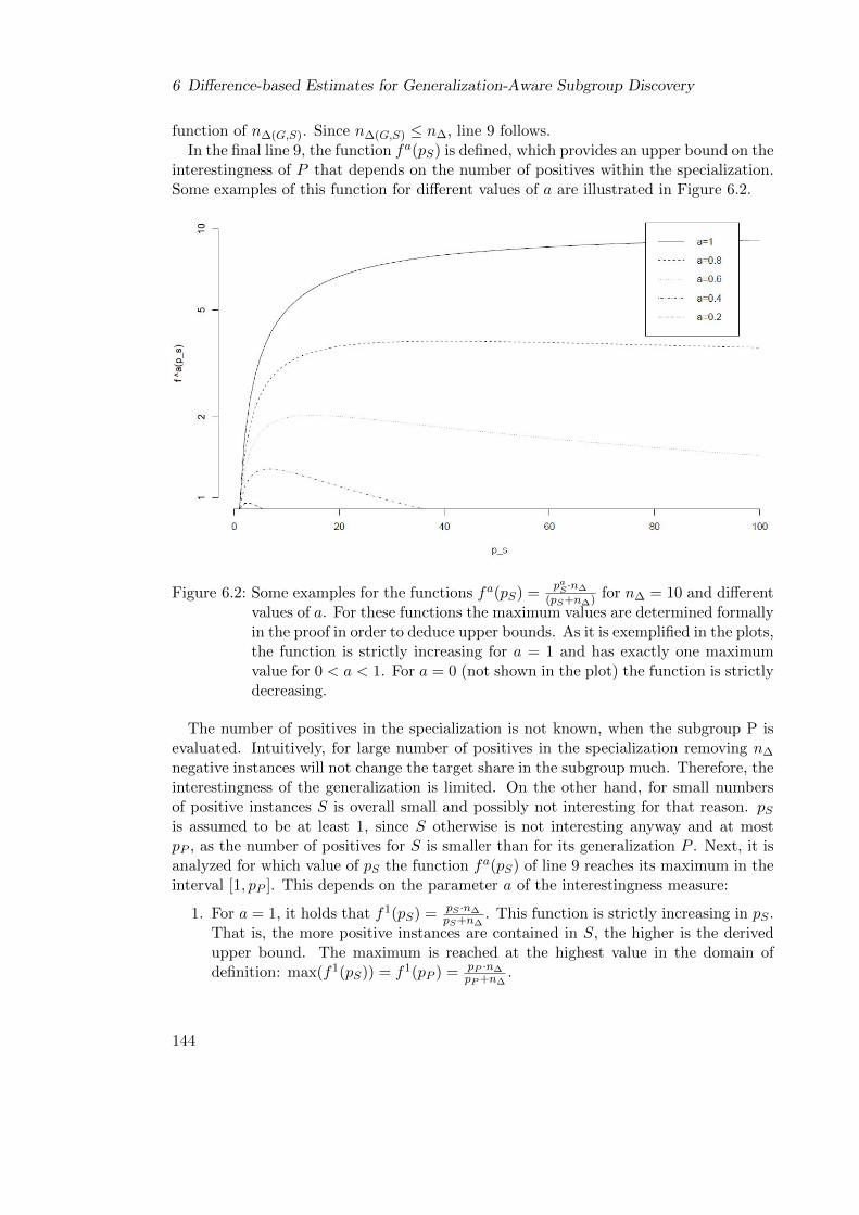
6 Difference-based Estimates for Generalization-Aware Subgroup Discovery
function of n∆(G,S). Since n∆(G,S) ≤ n∆, line 9 follows.In the final line 9, the function fa(pS) is defined, which provides an upper bound on the
interestingness of P that depends on the number of positives within the specialization.Some examples of this function for different values of a are illustrated in Figure 6.2.
Figure 6.2: Some examples for the functions fa(pS) =paS ·n∆
(pS+n∆) for n∆ = 10 and differentvalues of a. For these functions the maximum values are determined formallyin the proof in order to deduce upper bounds. As it is exemplified in the plots,the function is strictly increasing for a = 1 and has exactly one maximumvalue for 0 < a < 1. For a = 0 (not shown in the plot) the function is strictlydecreasing.
The number of positives in the specialization is not known, when the subgroup P isevaluated. Intuitively, for large number of positives in the specialization removing n∆
negative instances will not change the target share in the subgroup much. Therefore, theinterestingness of the generalization is limited. On the other hand, for small numbersof positive instances S is overall small and possibly not interesting for that reason. pSis assumed to be at least 1, since S otherwise is not interesting anyway and at mostpP , as the number of positives for S is smaller than for its generalization P . Next, it isanalyzed for which value of pS the function fa(pS) of line 9 reaches its maximum in theinterval [1, pP ]. This depends on the parameter a of the interestingness measure:
1. For a = 1, it holds that f1(pS) = pS ·n∆pS+n∆
. This function is strictly increasing in pS .That is, the more positive instances are contained in S, the higher is the derivedupper bound. The maximum is reached at the highest value in the domain ofdefinition: max(f1(pS)) = f1(pP ) = pP ·n∆
pP+n∆.
144

6.2 Estimates for Generalization-Aware Subgroup Mining
2. In contrast for a = 0, f0(pS) = n∆pS+n∆
is strictly decreasing. Thus, the maximum
value of f0 is reached for pS = 1, the minimum possible value of pS : max(f0(pS)) =f0(1) = n∆
1+n∆.
3. For 0 < a < 1, fa reaches a maximum for a certain value p∗ within the domainof definition. To determine that, the first derivative of fa is calculated using thequotient rule.
d
d pSfa(pS) = n∆ ·
d
dpS
paSpS + n∆
= n∆ ·(n∆ + pS) · a · pa−1
S − paS(n∆ + pS)2
= n∆ · pa−1S
an∆ + a · pS − pS(n∆ + pS)2
:= (fa)′
The only root of this derivative is at p∗ := a·n∆1−a . As can be easily shown, (fa)′(pS)
is greater than zero for pS smaller than p∗ and lower than zero for pS greater thanp∗. Therefore, p∗ is the only maximum of fa(pS). Thus, if pP > p∗, then p∗ is themaximum value of fa, otherwise the maximum is reached at the highest value ofthe domain of definition: max(fa(pS)) = fa(p) = pa·n∆
p+n∆,with p = min(a·n∆
1−a , pP ).
Overall, for any specialization S it holds that rabin(S) ≤ fa(pS) ≤ max fa(pS) =oerbina (P ), with the function maxima as described above, therefore oerbina (P ) asdefined in the theorem is a correct optimistic estimate. �
For any pair of two generalizations of P as well as for any pair of P and one of itsgeneralization (if P = P ′), this theorem provides an optimistic estimate of P . Theoptimistic estimate bound is dependent on the number of positives in the subgroupand the difference of negative instances between P ′ and P ′′. It is low if either thereare only few positives in P or the difference of negative instances between the pair ofgeneralizations is small (or a combination of both). Since the number of positives inP is independent of the chosen pair P ′, P ′′, the pair with the minimum difference ofnegative instances implies the tightest upper bound, which should be used to maximizethe effects of pruning.
As a special case, the theorem includes that the interestingness score of any subgroupis ≤ 0 if n∆ is 0. To the author’s knowledge, it is the first measure that includes thesedifferences in optimistic estimate bounds for subgroup discovery.
In some situations, this theorem provides significantly tighter bounds than the tradi-tional approach of Theorem 2, as can be observed in the following example:
Example 17 As in the previous example, assume that the subgroup A covers 20 posi-tive and 10 negative instances and the evaluation of the pattern A ∧ B shows that thissubgroup covers 16 positive and 8 negative instances. As interestingness measure thesubgroup discovery task uses r0.5
bin(P ). Then, Theorem 3 can be used to derive an opti-mistic estimate bound for the subgroup A∧B: The required statistic p is determined as
145

6 Difference-based Estimates for Generalization-Aware Subgroup Discovery
p = min(a·n∆1−a , pA∧B) = min(0.5·(10−8)
1−0.5 , 16) = 2. The optimistic estimate bound is then:
oer0.5bin(A∧B) = pa·n∆
p+n∆= 20.5·2
2+2 =√
22 .
The traditional bound from Theorem 2 depends on the maximum target share in thegeneralizations of A ∧ B. If this value is for example at 20%, then the derived upperbound for the subgroup A ∧ B takes the value 3.2 as computed in Example 15. This issignificantly less tight than the novel bound from Theorem 3. This can be explained bythe fact that only the novel bound exploits that the subgroup A∧B and its generalizationA differ only by a few negative instances. 2
6.2.4 Difference-based Optimistic Estimates for Numeric Targets
A related approach can be used to obtain optimistic estimates for generalization-awareinterestingness ranum = iP
a · (µP −maxH⊂P
µH) in settings with numeric target concepts:
Theorem 4 In a task with a numeric target concept, consider the pattern P with iPinstances and a maximum target value of maxP . P ′ ⊆ P is either P itself or one ofits generalizations and P ′′ ⊂ P ′ is a generalization of P ′. Let i∆ = |∆(P ′′, P ′)| be thenumber of instances contained in P ′′, but not in P ′ and min∆ the minimum target valuecontained in ∆(P ′′, P ′). Then, an optimistic estimate of P for the generalization awareinterestingness measure ranum is given by:
oeranum(P ) = max(0, oe′ranum(P )),
oeranum(P )′ =
i∆·iPiP+i∆
· (maxP −min∆), if a = 1i∆
1+i∆· (maxP −min∆), if a = 0
ia·i∆i+i∆
· (maxP −min∆), with i = min(a·i∆1−a , iP ), else
2
Proof Consider any specialization S ⊃ P and its generalization G = γ(S) accordingto Lemma 2. Then one can estimate the interestingness of S:
ranum(S) = iSa · (µS −max
H⊂SµH) (6.1)
≤ iS a · (µS − µG) (6.2)
= iSa ·
(∑c∈sg(S) T (c)
iS−∑
c∈sg(S) T (c) +∑
c∈∆(G,S) T (c)
iS + i∆(G,S)
)(6.3)
= iSa−1 ·
∑c∈sg(S)
T (c)−iS ·
(∑c∈sg(S) T (c) +
∑c∈∆(G,S) T (c)
)iS + i∆(G,S)
(6.4)
= iSa−1 ·
(i∆(G,S)
∑c∈sg(S) T (c)− iS
∑c∈∆(G,S) T (c)
iS + i∆(G,S)
)(6.5)
≤ iS a−1 ·
i∆(G,S) · iS ·maxc∈S
T (c)− iS · i∆(G,S) · minc∈∆(G,S)
T (c)
iS + i∆(G,S)
(6.6)
146

6.3 Algorithm
=i∆(G,S) · iS a
iS + i∆(G,S)·(
maxc∈S
T (c)− minj∈∆(G,S)
T (c)
)(6.7)
≤ i∆ · iS a
iS + i∆· (maxP −min∆) = fa(iS) · (maxP −min∆) (6.8)
In line 2, it is used that G is a generalization of S. Then it is exploited that sg(G) =sg(S) ∪∆(G,S), S ∩∆(G,S) = ∅. Line 6 exploits that the sum of any set of values isbigger than the minimum appearing value times the size of the set, but smaller than themaximum appearing value times the size of the set. Line 8 utilizes that i∆(G,S) ≤ i∆.fa is a function over the unknown number of all instances in the specialization, which
can be any number in [1, iP ]. fa is always positive. Therefore, if (maxP −min∆) ≤ 0,the optimistic estimate is given by 0. Else, the maxima of fa, which have already beenderived in the proof of Theorem 2, determine the bound: fa(iS) is strictly increasing fora = 1, strictly decreasing for a = 0 and reaches a maximum at a·i∆
1−a or at iP otherwise.Thus: ranum(S) ≤ (fa(iS)) · (maxP −min∆) ≤ max(fa(iS) · (maxP −min∆). The boundsfollow directly from inserting the respective maximum values. Since this holds for anyspecialization S of P , oeranum(P ) is a correct optimistic estimate for P . �
Similar to the optimistic estimate in the binary case, the derived optimistic estimate islow, if either the number of instances covered by P is low, or if the difference between thenumbers of instances covered by the generalizations P ′′ and P ′ is low (or a combinationof both). However additionally, the bound also considers the range of the target variablein these patterns, that is, the maximum occurring target value in P and the minimumtarget value in the difference set of instances. As a result, the bound becomes zero if theminimum target value removed by adding a selector to a generalization of P was higherthan the maximum remaining target value in P .
6.3 Algorithm
The presented optimistic estimates can in general be applied in combination with anysearch strategy. This chapter focuses on adapting an exhaustive algorithm, i.e., apriori [4,135], see also Chapter 3 for a detailed description of the base algorithm. This approachis especially suited for the task of generalization-aware subgroup discovery, since itslevelwise search strategy guarantees that specializations are always evaluated after theirgeneralizations and the highest target share found in generalizations can efficiently bepropagated from generalizations to specializations, see [29]. Therefore, and for bettercomparability with previous approaches, apriori was chosen as a basis for the novelalgorithm presented here. Using the following adaptations the algorithm is not onlycapable of determining the proposed optimistic estimates. The algorithm also propagatesthe required information very efficiently. The algorithmic adapations are described forthe binary case first.
Apriori performs a levelwise search, where new candidate patterns are generated fromthe last level of more general subgroups. In the adaptation of the algorithm, additionalinformation is stored for each candidate. This includes the maximum target share in
147

6 Difference-based Estimates for Generalization-Aware Subgroup Discovery
generalizations of this subgroup, the minimum number of negatives covered by any gen-eralization and the minimum number of negatives that were removed in generalizationsof this subgroup. After the evaluation of a subgroup the number of positives, the numberof negatives and the resulting target share are additionally saved in each candidate. Theminimum number of negative instances in a generalization is required to compute theminimum number of instances, which are contained in the subgroup, but not in a gener-alization. The other statistics are directly required to compute either the interestingnessscore or the optimistic estimates of the subgroup.
Whenever a new candidate subgroup P is generated in apriori, it is checked if all itsdirect generalizations G are contained in the candidate set of the previous level. Duringthis check, the statistics for the maximum target share in generalizations, the minimumnumber of negatives in a generalization and the minimum number of negatives that wereremoved in any generalization of this subgroup are computed by using the informationstored in the generalizations and applying simple minimum/maximum functions. Indoing so, the statistics required to compute the interestingness score of the subgroupand the optimistic estimates are propagated very efficiently from one level of subgroupsto the next level of more specific subgroups.
In the evaluation phase (the counting phase in classical apriori), each candidate isscored with respect to the applied interestingness measure. This requires to deter-mine the coverage of the subgroup. Combined with previously computed statisticsabout generalizations this is used to compute the interestingness according to the chosengeneralization-aware measure. Subgroups with sufficient high scores are placed in theresult set, potentially replacing others in a top-k approach. Afterwards the target sharein generalizations and the minimum number of removed negative instances are updatedby using the statistics of the current subgroup’s coverage. After the evaluation of asubgroup all optimistic estimates, that is, traditional estimates (see Theorem 2) anddifference-based estimates are computed from the information stored for a candidate. Ifany optimistic estimate is lower than the threshold given by the result set for a top-ksubgroup, then the subgroup is removed from the list of current candidates. Thus, nospecializations of this subgroup are explored in the next level of search.
The approach for numeric target concepts is very similar, except that minimum/maxi-mum and mean target values as well as overall instance counts of the candidate subgroupare stored instead of counts of positives and negatives. When determining the pruningbounds, a subgroup is compared with all its direct generalizations. For each general-ization, an optimistic estimate bound is computed based on the difference of instancesbetween the generalization and the specialization and the stored minimum/maximumtarget values. The tightest bound can be applied for pruning.
148

6.4 Evaluation
6.4 Evaluation
This section demonstrates the effectiveness of the presented approach in an evaluationusing well-known datasets from the UCI [13] repository2. As a baseline algorithm avariant of the MPR-algorithm presented in [29] is used as the current state-of-the-artalgorithm for this setting. The algorithm was slightly modified in order to support top-kmining and to incorporate the bounds of Theorem 2 for any a. Since this algorithmfollows the same search strategy as our novel algorithm, that is, apriori, this allows todetermine the improvements that originate directly from the advanced pruning boundspresented in this work. For the experiments, the algorithms were implemented as a pluginin the open-source environment VIKAMINE 2, see Chapter 8. The implementationutilizes an efficient bitset-based data structure to determine the coverage of subgroups.Results below are shown for k = 20, a realistic number for practical applications, whichwas also used for example as beam size in [274]. Different choices of k lead to similarresults. For the numeric attributes an equal-frequency discretization was used, using allhalf-open intervals from the cutpoints and the intervals between two adjacent cutpointsas selectors. The experiments were performed on an office PC with 2.8 Ghz and 6 GBRAM.
The first part of the evaluation compared the runtimes of the presented algorithmfor binary target concepts using different generalization-aware interestingness measuresrabin, see Table 6.1 and Table 6.2.
The results in Table 6.1 show that utilizing difference-based pruning leads to signifi-cant runtime improvements in almost all tasks. The runtime improvements tend to belarger for higher parameters of a, since pruning can be applied more effectively if theinterestingness measures favors larger subgroups. The improvements are explained bythe fact that by exploiting the additional pruning options substantially less candidateshave to be evaluated, see Table 6.2. This direct dependency between the number ofevaluated candidates and runtime can also be observed for the subsequent experiments,for which the candidate numbers will not be listed separately.
Some datasets in particular showed massive runtime improvements, e.g., the datasetsionosphere, spammer or segment. For a more detailed analysis, these tasks were inves-tigated more closely. It turned out that the search space for these datasets containsmultiple selectors that cover a vast majority of the instances. Conjunctive combinationsof subsets of these selectors still cover a large part of the dataset and especially of thepositive instances. As traditional optimistic estimates are based on this number of cov-ered positive instances, pruning cannot be applied on these combinations efficiently. Incontrast, since the number of negative instances, by which those patterns differ fromgeneralizations, is often very low in these cases, such combinations can be pruned oftenusing the difference-based optimistic estimates presented in this work. This leads to themassive improvements. It can be concluded that our new pruning scheme is especiallyefficient if many selectors cover a majority of the dataset. In some cases, the algorithms
2Additionally, the dataset spammer is derived from the publicly available data from the ECML/PKDDdiscovery challenge 2008, see also Section 7.7.4.
149

6 Difference-based Estimates for Generalization-Aware Subgroup Discovery
Table 6.1: Runtime comparison (in s) of the base algorithm with traditional pruningbased on the positives (std) and the novel algorithm with additional difference-based pruning (dbp) using different size parameters a for interestingness mea-sures rabin. The maximum number of describing selectors was limited to d = 5.“-” indicates that the algorithm did not finish due to lack of memory.
a 0.0 0.1 0.5 1.0Pruning dpb std dpb std dpb std dpb std
adults 0.9 0.9 16.5 40.8 1.0 6.8 0.6 1.3audiology < 0.1 0.1 < 0.1 < 0.1 < 0.1 < 0.1 < 0.1 < 0.1autos 0.4 - 0.3 30.6 0.1 16.0 < 0.1 1.7census-kdd 15.4 15.2 1103.5 - 46.0 245.9 16.1 28.2colic 0.1 < 0.1 0.6 1.1 0.2 1.6 0.1 0.5credit-a < 0.1 < 0.1 0.7 1.7 0.2 1.8 < 0.1 0.3credit-g 0.2 0.1 14.3 26.4 3.8 25.7 0.4 4.2diabetes 1.3 5.3 8.0 19.6 1.8 16.2 0.1 1.2hepatitis 0.3 6.4 0.7 1.6 0.1 1.3 < 0.1 0.2hypothyroid < 0.1 0.6 0.2 2.2 0.2 1.7 < 0.1 0.6ionosphere 0.1 0.1 148.4 - 0.3 - 0.1 102.2spammer 1.5 1.9 277.8 - 12.1 412.8 0.5 41.4segment 31.5 - 5.5 317.4 0.1 69.3 < 0.1 12.1
Table 6.2: Comparison of the number of evaluated candidates in the base algorithm withtraditional pruning based on the positives (std) and in the novel algorithmwith additional difference-based pruning (dbp). Each double column uses adifferent size parameter a for the interestingness measures rabin. The maximumnumber of describing selectors was limited to d = 5. “-” indicates that thealgorithm did not finish due to lack of memory.
a 0.0 0.1 0.5 1.0Pruning dpb std dpb std dpb std dpb std
adults 66,909 148,408 1,272,897 4,559,066 76,280 773,210 14,456 123,321audiology 10,950 46,390 6,349 13,791 6,349 13,791 6,387 13,829autos 209,553 - 47,422 6,387,287 31,320 4,410,259 16,783 626,939census-kdd 82,215 164,430 22,400,736 - 815,878 6,140,536 88,276 461,130colic 6,903 13,806 109,323 404,352 80,074 563,018 29,377 192,550credit-a 4,186 8,372 146,824 595,565 95,036 683,878 10,986 118,741credit-g 68,806 149,175 2,496,144 7,834,159 1,104,248 6,837,491 176,187 1,444,033diabetes 449,096 2,183,798 1,527,242 5,755,861 560,236 4,643,343 26,482 423,433hepatitis 115,483 2,105,085 168,461 642,124 56,970 533,107 8,573 74,797hypothyroid 14,994 178,394 42,049 555,357 62,195 564,959 8,945 186,236ionosphere 56,956 114,587 22,724,266 - 80,483 - 62,881 20,680,731spammer 171,565 390,367 13,127,644 - 1,237,991 14,567,622 14,669 3,922,800segment 6,591,619 - 924,140 26,802,236 34,946 11,920,849 19,514 3,045,612
150

6.4 Evaluation
did not finish due to out-of-memory errors despite the large amount of available memory.This occurs less often using the novel bounds, see for example the results for the vehicledataset, since less candidates are generated and have to be stored in apriori.
In the second part of the evaluation, the interestingness measure r0.5bin, a generalization-
aware variant of the binomial-test, was further analyzed by comparing the runtimesfor different search depth (maximum number of selectors in a subgroup description),see Table 6.3. As before, almost all tasks finished earlier using the novel difference-based pruning. While the improvement is only moderate for low search depth, massivespeedups can be observed for d = 5 and d = 6. For d = 6, several runs with onlytraditional pruning did not finish because of limited memory. This did not happen forthe datasets in the experiments if the additional pruning was applied.
Table 6.3: Runtime comparison (in s) of the base algorithm with traditional pruningbased on the positives (std) and the novel algorithm with additional difference-based pruning (dbp) using different maximum numbers d of describing selec-tors in a pattern. As interestingness measure the generalization-aware meantest r0.5
bin was used. “-” indicates that the algorithm did not finish due to lackof memory.
d 3 4 5 6Pruning dpb std dpb std dpb std dpb std
adults 0.7 0.8 0.9 1.6 1.0 6.8 1.3 26.7autos < 0.1 0.1 0.1 1.5 0.1 16.0 0.2 182.4census-kdd 16.6 17.5 26.0 48.1 46.0 245.9 79.8 6392.5colic 0.1 0.1 0.2 0.5 0.2 1.6 0.3 3.6credit-a < 0.1 0.1 0.1 0.4 0.2 1.8 0.3 5.5credit-g 0.2 0.2 1.2 2.6 3.8 25.7 6.3 235.1diabetes 0.1 0.1 0.6 1.6 1.8 16.2 3.6 91.9hepatitis < 0.1 < 0.1 0.1 0.3 0.1 1.3 0.2 4.4hypothyroid < 0.1 0.1 0.1 0.4 0.2 1.7 0.2 6.3ionosphere 0.1 1.2 0.1 31.7 0.3 - 0.1 -spammer 1.0 1.4 3.5 13.4 12.1 412.8 30.2 -segment 0.1 0.2 0.1 3.9 0.1 69.3 0.1 -
In the last part of the evaluation, the improvements in a setting with numeric targetconcepts and interestingness measures ranum(P ) were examined. For subgroup discoverywith numeric targets and generalization-aware interestingness measures, no specializedoptimistic estimates have been proposed so far. To allow for a comparison nonetheless,the optimistic estimate bound oe1
num =∑
c:T (c)>µ∅
(T (c)−µ∅) is used, which has been shown
to be a correct optimistic estimate for the non-generalization-aware measure q1num(P ) =
iPa · (µP − µ∅) [249]. Since ranum(P ) ≤ r1
num(P ) ≤ q1num(P ), this can also be used as
a (non-tight) optimistic estimate for any generalization-aware interestingness measureranum. Using the considerations of Chapter 4 more sophisticated bounds could be derived
151

6 Difference-based Estimates for Generalization-Aware Subgroup Discovery
to further decrease runtimes, but for better comparability the experiments focus on thisestablished bound.
Results are shown in Table 6.4 and Table 6.5. Since the applied traditional boundis tight for a = 1, the runtimes in this case are already relatively low for the studieddatasets with traditional pruning, leaving only little room for improvement. For lowervalues of a, significant runtime improvements can be observed, which reach a full orderof magnitude (e.g., for the datasets concrete data and housing). The average relativeruntime improvement is on average highest for a = 0.5. This can be explained by thefact that for lower values of a even small subgroups can be considered as interesting.This makes it more difficult to exclude subgroups from search by pruning also whenusing the difference based bounds. As in the binary case, the advantages of improvedpruning increase for higher search depths, cf. Table 6.5.
Table 6.4: Runtime comparison (in s) of the base algorithm with traditional pruningbased on the instances covered by a subgroup only (std) and the novel al-gorithm with additional difference-based pruning (dbp) for numeric targetconcepts. Each double column corresponds to a different size parameter afor the interestingness measure ranum. The maximum number of describingselectors was limited to d = 5. “-” indicates that the algorithm did not finishdue to lack of memory.
a 0.0 0.1 0.5 1.0Pruning dpb std dpb std dpb std dpb std
adults 17.0 71.0 19.9 73.7 11.4 49.9 3.9 11.6autos 2.8 - 5.5 - 0.7 - < 0.1 0.9breast-w 0.5 2.1 0.9 2.2 0.1 1.3 < 0.1 0.1concrete data 8.5 42.1 11.7 47.7 2.1 29.6 0.1 0.6credit-a 1.3 5.6 1.9 5.9 1.1 4.7 0.1 0.4credit-g 3.4 21.8 5.7 23.1 4.1 16.2 0.2 0.5diabetes 4.3 22.8 6.0 25.1 5.0 20.0 0.4 0.9forestfires 1.9 7.5 2.8 7.9 2.2 6.8 2.4 4.9glass 1.7 19.4 2.4 19.3 0.3 7.3 < 0.1 0.2heart-c 2.7 7.1 3.6 7.7 1.8 6.1 0.1 0.3housing 3.2 43.6 5.5 46.0 2.8 38.4 0.2 5.7yeast 3.3 13.7 4.3 14.5 1.7 10.4 0.1 1.3
Overall, the evaluation results clearly indicate that the difference-based pruningthat is introduced in this work substantially improves the runtime performance forgeneralization-aware subgroup discovery. The effects are especially beneficial, if thedataset contains selectors, which cover a majority of the dataset or if the maximumsearch depth of the discovery task is high.
152

6.5 Summary
Table 6.5: Runtime comparison (in s) of the base algorithm with traditional pruningbased on the instances covered by a subgroup only(std) and the novel al-gorithm with additional difference-based pruning (dbp) for numeric targetconcepts. Each double column corresponds to a different maximum numberd of describing selectors for a subgroup. As interestingness measures thegeneralization-aware mean test r0.5
num was used. “-” indicates that the algo-rithm did not finish due to lack of memory.
d 3 4 5 6Pruning dpb std dpb std dpb std dpb std
adults 1.9 2.2 5.5 11.0 11.4 49.9 17.4 263.4autos 0.2 0.5 0.5 13.2 0.7 - 0.7 -breast-w < 0.1 < 0.1 0.1 0.3 0.1 1.3 0.1 6.0concrete data 0.3 0.3 1.0 2.9 2.1 29.6 3.3 -credit-a 0.1 0.1 0.5 0.8 1.1 4.7 1.7 24.3credit-g 0.3 0.2 1.3 2.1 4.1 16.2 7.4 99.1diabetes 0.2 0.2 1.4 2.0 5.0 20.0 10.5 189.8forestfires 0.2 0.2 0.9 1.4 2.2 6.8 5.3 59.6glass 0.1 0.1 0.2 0.9 0.3 7.3 0.3 80.5heart-c 0.1 0.1 0.5 0.8 1.8 6.1 3.6 43.4housing 0.2 0.2 1.0 2.6 2.8 38.4 5.6 -yeast 0.2 0.2 0.7 1.6 1.7 10.4 2.7 77.6
6.5 Summary
In this chapter, a new scheme of deriving optimistic estimates bounds for subgroup dis-covery with generalization-aware interestingness measures was proposed. In contrast toprevious approaches on deriving optimistic estimate bounds, these are not only basedon the anti-monotonicity of instances covered by a subgroup. Instead, they incorporatealso the number of instances, which are covered by the subgroup, but not by its general-ization. The optimistic estimates have been incorporated in an efficient algorithm thatoutperforms previous approaches, in many cases by more than an order of magnitude.The speed-up is especially high if the dataset contains selection expressions that covera large part of the dataset.
153


7 Local Models for Expectation-DrivenSubgroup Discovery1
This chapter introduces a novel family of interestingness measures, which enables theidentification of previously undiscovered interesting subgroups and avoids uninterestingfindings. This is accomplished by estimating the target share of a subgroup, which a dataanalyst would expect if statistics related to this subgroup are available. Deviations fromthese expectations are then considered as interesting. The novel interestingness mea-sures can be formalized in a general framework, which also includes previously proposedmeasures as a special case.
7.1 Approach and Motivation
A key issue of subgroup discovery is to find appropriate interestingness measures, whichselect subgroups with an interesting target share. For that purpose, the share of thetarget concept in a subgroup is traditionally compared with the target share in the over-all dataset. This chapter argues that this leads to subgroups that might be consideredas uninteresting by users, as their target share is expected considering the effects of theinfluence factors that are combined in this subgroup. This problem is approached byadapting interestingness measures, such that subgroups are not scored isolated from eachother. Instead, statistics of the influence factors that are combined in a subgroup areused to model the user’s expectation of the target share in this subgroup considering theinteraction of the influence factors with each other and the target concept. Then, thecomparison between a subgroup’s target share and the target share in the total popu-lation is replaced with a comparison to the formed expectation. In doing so, subgroupsare selected, for which the actual target share deviates from the user’s expectation.
As the expectation of a user is subjective, it is certainly not possible to capture it in onesingle mathematical function. Instead, this chapter introduces methods that find values,which are plausible and in line with human reasoning. Fortunately, a related task hasbeen studied in depth in another research field before, that is, the research on graphicalknowledge representations and in particular the elicitation of probability tables for themanual construction of bayesian networks. In this work, it is shown how techniques fromthis field can be transferred to subgroup discovery: Fragments of bayesian networks aregenerated for each candidate subgroup in order to capture the dependency between theinfluence factors and the target concept. This is used to determine plausible expectations
1The approach presented in this chapter has previously been published as [176]: Florian Lemmerichand Frank Puppe: Local Models for Expectation-Driven Subgroup Discovery. In Proceedings of the11th International Conference on Data Mining (ICDM), 2011.
155

7 Local Models for Expectation-Driven Subgroup Discovery
for complex subgroups, that is, subgroups with conjunctive descriptions of more thanone selector.
The contribution of this chapter is threefold: First, a formal generalization of tra-ditional subgroup discovery is presented that allows for expectation-aware evaluationof subgroups. Second, several practical methods are presented to approximate humanexpectations for a subgroup’s target share by constructing fragments of bayesian net-works as local models. Third, the effectiveness of the presented techniques is evaluatedin several experiments including two real-world case studies.
The approach of expectation-driven subgroup discovery is motivated in a two-partexample:
Example 18 For an imaginary medical domain, consider the influence factors (sub-groups) presented in Table 7.1.
Table 7.1: Motivational examples.
Influencing factors Share of target concept
∅ (population) 0.5S 0.1P 0.3S ∧ P 0.5
∅ (population) 0.5A 0.7B 0.7C 0.5A ∧B 0.75A ∧ C 0.75
The target concept describes the success of some treatment of a primary disease. Theaverage success rate in the total population is 0.5. S is a secondary disease that lowersthe chance of healing to 0.1. P is a pharmaceutical that is used only in difficult cases. Asin these cases the treatment tends to be less successful, the share of the target conceptgiven treatment with P is lower than in the overall population, it is at 0.3. Anyway,P helps in particular people that suffer also from the disease S, so in this case thesuccess rate is at 0.5. This subgroup is probably interesting to domain experts, whichare unaware of the interaction between S and P that leads to an unexpected high targetshare. In traditional subgroup discovery the subgroup S ∧ P , which describes patientssuffering from S and also receive treatment P , is considered as uninteresting and is notdiscovered, because it does not have a higher share of the target concept in comparisonto the overall dataset. In contrast to this, the novel approach presented in this chapterwill formalize that the combination of S and P is expected to lead to a target sharebelow 0.5, since both influence factors lead to a decrease of the target share individually.Therefore, the subgroup S ∧ P is reported as interesting, as its target share is aboveexpectation.
156

7.2 Related Work
For the second part of the example, consider three other influence factors A, B andC, for which no interaction is previously known. The presence of either A or B increasesthe likelihood of a successful treatment from 0.5 to 0.7. The presence of C alone doesnot influence the target share. If A occurs together with B or together with C, then thetarget share is increased to 0.75. Since B leads to an increase of the target share in thetotal population, it is not surprising that it also leads to an increase for the patients,which are influenced by A. Thus, for A ∧ B a target share, which is higher than thetarget share of A alone, could be expected. In contrast, C alone does not alter the targetshare of successful treatments. Given only this information, one would also expect noeffect of C in the subpopulation of patients with influence factor A. But this is not thecase in the example. As a consequence, the subgroup A∧C is probably more interestingto users than the subgroup A ∧ B. This is not reflected in traditional interestingnessmeasures for subgroup discovery, even if extensions for minimum improvements are used,cf. Section 2.5.4. For many applications, it is also not important that experts do not knowthe statistics for the single influence factors A, B or C beforehand: If a subgroup suchas A ∧B is reported as interesting, then the data analysts will request and incorporatestatistics for the single influence factors in the assessment of the discovered subgroups.2
The remainder of this chapter is structured as follows: Section 7.2 discusses relevantrelated work. Next, the general idea of the novel approach, expectation-driven sub-group discovery, is presented in Section 7.3. Section 7.4 introduces, how techniques frombayesian network research can be transfered to this setting. Afterwards, several possi-bilites to compute expectations in practice are presented in Section 7.5. In Section 7.6computational issues are outlined. Then, Section 7.7 describes several experiments thatshow the effectiveness of our approach. A discussion of potential problems and possibleimprovements to the novel approach is provided in Section 7.8. Finally, the main resultsof this chapter are summarized in Section 7.9.
7.2 Related Work
Since selecting the most interesting patterns is a key issue for subgroup discovery, alarge variety of interestingness measures has been proposed for this task. These aresummarized in Section 2.5.3. Most of these measures focus exclusively on the statisticsof the evaluated subgroup and do not incorportate statistics of other related subgroups.
Several improvements have been suggested in the past to avoid redundant results,which can be explained by other parts of the result, but most of them focus on the coverof the subgroups [91, 95, 104], see Section 2.5.5 for more details. However, in manyapplications it is preferred to report several subgroups as influencing factors on thetarget concept, even if they describe overlapping subpopulations, since domain expertsmight be unaware of this co-occurrence.
Considering adaptations based on the subgroup descriptions, it was proposed in [35] toapply a constraint on the minimum improvement for rule discovery. This constraint oftenleads to more useful results, but as demonstrated in the introduction it may suppressinteresting subgroups and it may also still include predictable ones. This approach was
157
7 Local Models for Expectation-Driven Subgroup Discovery
adapted in [29, 30] to include only subgroups with a statistically significant improvementover all generalizations, but this approach in general suffers from the same problems.Grosskreutz et al. presented a case study [102], in which they applied the minimumimprovement function not as a constraint, but as a modified interestingness measure.This approach can be seen as a special case of the more general framework presented inthis work. For more details on approaches in this direction, we refer to Section 2.5.4.
In the context of exception rule mining, Hussain et al. proposed another approach thatscores the interestingness of a rule with respect to its generalizations, if these are alreadyknown common sense rules [124]. Their approach is difficult to comprehend for domainexperts, and unlike our approach, it can not be generalized. Freitas proposes an adaptionto interestingness measures that aims at including the attribute surprisingness [81]. Incontrast to the novel approach of this work, this method is not suited to combine factorswith opposing influences on the target concept and can also not be generalized.
For the related field of itemset mining, Tatti [235] uses entropy-based flexible modelsto determine itemsets that have a surprising support given its sub-itemsets. In the samearea, Webb proposed an approach in which only those itemsets are considered as inter-esting that have higher support than expected under the assumption of independence inany partition of the itemsets [253]. Regarding this independence assumption as a verysimple local model, the approach proposed in this work could be seen as a transfer ofthis general idea to the field of subgroup discovery. However, this transfer is non-trivial,since obviously each interesting subgroup implies an immediate dependency between thetarget concept and the variable describing a subgroup. Therefore, in this work it is pro-posed to utilize an independence of the influences on the target concept instead of anindependence of the selectors/itemsets. Local models are used to determine the effectsof these independent influences.
Estimating the probability distribution of a target variable given only some conditionalprobabilities and measuring the interaction of their influence are well studied problemsin the field of bayesian networks. To the best of our knowledge, these estimations havenot yet been used in interestingness measures for subgroup discovery. Bayesian networkshave been proposed to store background knowledge and to find patterns deviating fromthis background knowledge by Jaroszewicz et al., but their approach includes no explicitmechanisms to avoid uninteresting combinations of influencing factors [127]. De Bie et al.proposed a general framework for pattern mining, in which prior information is encodedin a data model [40]. Then, maximally informative patterns with respect to this modelare selected. While this work mainly follows a similar general idea, its focus on subgroupdiscovery and local data models allows for an easy application in practice. Recently,Kontonasios et al. summarized several approaches, which aim at mining “unexpectedpatterns” [153]. These techniques are concerned with integrating background knowledgein the discovery process. In contrast, the novel approach presented in this work doesnot rely on background knowledge, but only on the dataset itself.
158

7.3 A Generalized Approach on the Subgroup Discovery Task
7.3 A Generalized Approach on the Subgroup Discovery Task
This section presents a novel, generalized approach to construct interestingness measuresfor subgroup discovery. It is based on the expectations of users regarding the targetshares for subgroups with complex descriptions, i.e., subgroup descriptions with morethan one selector.
The approach is based on the following observations of the domain experts behaviorduring the analysis of subgroup discovery results:
1. Subgroups with conjunctive descriptions are usually evaluated with respect to re-lated subgroups. In particular, the effects of the basic influence factors are inves-tigated in order to assess the combination of influence factors that describes thesubgroup. E.g., when a complex subgroup description A∧B is presented to domainexperts as a result of an automatic search, the experts additionally require to seestatistics of its generalization A and its generalization B for the introspection ofthis subgroup. These are used to study the interaction with each other and withthe target concept. As an alternative, it is inspected what effects a single influencefactor has in absence of other influences. That is, for the result subgroup A ∧ Balso the subgroups A ∧ ¬B and ¬A ∧B are considered.
2. Based on the knowledge of these statistics domain experts form an implicit orexplicit impression, what the target share in a subgroup “should” be at most.This expectation is partially subjective, but follows general intuitions. It may alsodepend on prior knowledge.
3. The assessment of a subgroup then compares the actual target share of a sub-group in the data and the expected target share. The subgroup is considered asinteresting if the formed expectation differs clearly from the actual target share.
To support this course of action in automated subgroup discovery, this work proposesto adapt the well-known Kloesgen measure qaKl(P ) = iP
a · (τP − τ∅), that depends onthe subgroup size iP , the target share in the subgroup τP and the target share in theoverall dataset τ∅. It is adjusted into the new family of interestingness measures qaexpχ :
qaexpχ(P ) = iPa · (τP − χ(P )), a ∈ [0, 1],
where the expectation function χ(P ) describes the expectation for the target share ofthe subgroup P that is formed by the inspection of related subgroups. The expectationvalue is the highest target share that can be explained by domain experts given thisinformation. To increase the acceptance of the results, it can be helpful to use a functionχ that is understandable for domain experts. Although additional background knowledgecould be integrated in this framework, this work focuses on expectation functions χ(P )that take only statistical information contained in the dataset into account.
It is not assumed that the domain experts know all statistics, which are utilized toform the expectation, in mind a-priori. However, if a subgroup would be presented inthe result set and then be analyzed by experts, then these statistics would be taken
159
7 Local Models for Expectation-Driven Subgroup Discovery
into account to examine this subgroup. From this point of view, the novel approach canbe considered as an anticipation of the subgroup analysis phase that follows the auto-matic subgroup discovery step: The automatic discovery integrates knowledge, whichwould come up in a more detailed introspection of a subgroup, directly into the inter-estingness measure and thus into the selection process of the automatic search. This isespecially important, as for many application scenarios the domain experts’ time is amajor limiting factor and the analysis of subgroups can be tedious, especially for com-plex patterns with more than one selector. Additionally, the novel approach enables theidentification of subgroups, which are interesting considering the additional information,but remain undetected using traditional subgroup discovery interestingness measures.This is exemplified in the case studies of Section 7.7. Although the general concept ofexpectation-driven subgroup discovery can also be extended to other types of attributes,this chapter is limited to a setting with binary target concepts only.
7.4 Expectations Through Bayesian Network Fragments
Since expectations are subjective, the expected target share χ(P ) can be determined inmany different ways. This work, however, focuses on models, which are inspired fromthe research on bayesian networks, cf. for example [206]. Bayesian networks are knowl-edge representations in form of probabilistic graphical models with directed and acyclicgraphs. In these models, attributes (random variables) of a dataset are representedby graph nodes. Interdependencies between attributes are specified by directed edgesbetween these nodes. Additionally each node has a corresponding conditional proba-bility table, which assigns a probability to each attribute value for each combination ofattribute values in the parent nodes.
Knowledge from domain experts can be utilized to construct bayesian networks. Tomake the knowledge acquisition process easier, different advanced techniques have beenproposed: For example, when building a bayesian network, the complete probabilitydistribution of an attribute must be specified in a conditional probability table. Thisis a difficult and tedious task for domain experts. In order to simplify the elicitationprocess, the entries of this table can be constructed with the input of only a few baseprobabilities. For instance, using such techniques the probability table of an attributecan be generated by providing only the probability distribution of this attribute for cases,in which exactly one of the binary parent attributes is set to true instead of specifyingthe distribution for all possible combinations of values in the parent attributes.
The problem of generating an expectation value for the target share of a subgroupP is transfered to the setting of bayesian networks as following: For each specializationS ⊂ P a small local model is constructed by partitioning the subgroup description Pinto the two factors A = S and B = P \S. Thus, the description of P is equal to A∧B.Each local model uses the simple graph structure of Figure 9.2.
It contains three nodes for A, B, and the target concept T and two edges, whichare directed from A and B to the target concept. The conditional probability table forthe target concept T then contains the values P (T |A,B), P (T |A, B), P (T |A, B) and
160

7.4 Expectations Through Bayesian Network Fragments
T
BA
Figure 7.1: Basic structure of the bayesian network fragment used as a local model todetermine plausible expectation values.
P (T |A, B). The entry P (T |A,B) is most important, as it is used as an estimation forthe target share in the subgroup described by A ∧ B, that is, the subgroup P . It isassumed that the other values of this probability table are known to the experts, as theyare a typical part of subgroup introspection. Based on these other values a plausibleestimate for P (T |A,B) is constructed, which is then compared with the actual targetshare for this subgroup.
Fortunately, the task of completing conditional probability tables that are plausibleand in line with human expectations under these circumstances has already been studiedin depth in the bayesian network community for the task of elicitation of probabilitytables by domain experts, see for example [259]. In this field several methods have beenproposed, which utilize an assumption of independence of the influences on the targetvariable (in contrast to the independence of the variables themselves). Other techniquesoriginate in the idea of measuring the causal interaction of two variables with respectto a target variable. One can then compute an estimation for P (T |A,B) by assumingthat this causal interaction is zero. The next section summarizes some of the suggestedapproaches to determine P (T |A,B).
By using these techniques, one local expectation value is obtained for each model, thatis, for each partition of the describing selectors. The expectation value for one modelwill be denoted as λ(A,B). For subgroups with larger subgroup descriptions, there ismore than one partition of this subgroup P in A and B. In this case the maximum ofthe expectations λ(A,P \A) is used as the result for the global expectation function:
χ(P ) = maxA⊂P
λ(A,P \A).
Thus, the global expectation value is the highest value that can be explained by theinteraction between a part of the influence factors of P and their complement (withrespect to the subgroup description). As an additional lower bound for this expectation,the minimum of target shares of all generalizations is used. That means that the targetshare of a subgroup is never considered as unexpectedly high if it is lower than the targetshare of all its generalizations.
161

7 Local Models for Expectation-Driven Subgroup Discovery
7.5 Expectations for Influence Combination
This section introduces different methods to compute an expectation for the target sharein practice. It first shows how existing techniques can be modeled as a special case ofthe previously presented formalization of expectation-driven subgroup discovery. Then,different local models λ(P ) are presented, which are used to generate more plausibleexpectation estimations of the target shares.
7.5.1 Classic Subgroup Discovery
The most simple case for an expectation function is to use the target share in the overalldataset τ∅ independent from the parent patterns A and B:
λclassicSGD(A,B) = τ∅
As a consequence, also the global expectation value is equal to the target share, sinceχ(P ) = maxA⊂P λ(A,P \A) = τ∅. In doing so, the unexpected patterns correspond ex-actly to the results of classic subgroup discovery with Kloesgen interestingness measuresqaKl. Thus, classic subgroup discovery is a special case of expectation-driven subgroupdiscovery presented in this work.
7.5.2 Minimum Improvement
The minimum improvement constraint is often applied as an additional constraint insubgroup discovery, cf. [35]. It implies that a subgroup is only considered as interestingif its target share is higher than the target shares of all its generalizations. Of course, theamount of the minimum improvement can be used itself as an interestingness measure, asit was done for example in [102, 29], see also Section 2.5.4. This family of interestingnessmeasures can be captured by the proposed framework using the expectation function
λ(A,B) = max (τA, τB) .
Thus, the global expectation is given by the maximum of all target shares τG in anygeneralization G of P: χ(P ) = maxG⊂P τG.
7.5.3 Leaky-Noisy-Or
The probably most popular model in bayesian network research to estimate the completeprobability table of an attribute from few base probabilities is the (leaky-)noisy-or model,see for example [116] or [115]. It assumes the so called independence of causal influence.In contrast to traditional statistical independence, this does not imply that there is nointeraction between the respective variables, but that the causal mechanisms by whichthey affect the target concept do not interact, cf. [69].
Using the noisy-or model for the graph structures of the local models, A and B areassumed to be the only two causes of T . They occur independently from each other andalso influence T independent from each other. In the leaky-noisy-or model, an extension
162
7.5 Expectations for Influence Combination
of noisy-or, all potential other causes are modeled in an additional independent variableX (“leak parent”). Each of these three variables can cause an intermediate (hidden)variable to be true. If any of these intermediate variables is true, then also the variablefor the target concept T is deterministically set to true. The value for P (T |A,B) from theconstructed table can then be considered as the estimation of the target share under theleaky-noisy-or assumption. As described for example in [202], the expectation estimationis computed as:
λLN−Or(P ) = P (T |A,B) = 1−(1− P (T |A, B)
)·(1− P (T |A, B)
)1−
(P (T |A, B)
) .
7.5.4 Additive Synergy and Multiplicative Synergy
Additive synergy and multiplicative synergy are measures for the combination of qualita-tive influence, see for example [185, 186]. Both are used to describe qualitative behaviorgiven two parent variables in a bayesian network. The additive synergy is defined byconditional probabilities as following:
SynAdd = P (T |A,B) + P (T |A, B)− P (T |A, B)− P (T |A, B)
If it is assumed that the influence of A and B is independent according to this measure,then the synergy is equal to zero: SynAdd = 0. Thus, a (local) expectation function forP (T |A,B) is derived by solving the equation for P (T |A,B):
P (T |A,B) = P (T |A, B) + P (T |A, B)− P (T |A, B) := λAdd
This follows the idea that if the presence of A alone increases the probability of Tby e.g., 5% and the presence of B alone increases the probability by e.g., 3%, then thepresence of A and B together should increase the probability of T by 5% + 3% = 8%.
Analogously, an expectation function can be constructed for the alternative measuremultiplicative synergy by replacing the sum in the above formula by the product, result-ing in:
P (T |A,B) =P (T |A, B) · P (T |A, B)
P (T |A, B):= λMult
Additive and multiplicative synergy are very easy to explain and using them to gen-erate expectation estimates can lead to interesting results. However, there are alsodownsides of this approach, in particular if two strong positive or two strong negativefactors are combined: In this case the computed value for the expectation deviates toomuch from the base target share. In extreme cases, values obtained by this formula evenexceed the limits zero and one, cf. also Section 7.7.2.
163

7 Local Models for Expectation-Driven Subgroup Discovery
7.5.5 Logit-Model
An alternative approach to measure causal interaction between influencing factors inbayesian networks is the loglinear or logit model, see [239]. A plausible estimation canbe obtained by assuming, that this causal interaction between the influence factors iszero. The probability P (T |A,B) can in this case be computed given the other entries ofthe conditional probability table.
In the logit model for bayesian networks, the conditional probability table for a binarynode with two binary parents is specified by a set of equations: log P (T |AB)
P (¬T |AB) = a + b ·z(A) + c · z(B), with A = {A, A},B = {B, B}, and z(X) = 1 iff X is true. In particular,this describes the following four equations:
logP (T |A, B)
P (¬T |A, B)= a
logP (T |A, B)
P (¬T |A, B)= a+ b
logP (T |A, B)
P (¬T |A, B)= a+ c
logP (T |A,B)
P (¬T |A,B)= a+ b+ c
Since probabilities for the value combinations (A, B), (A, B) and (A, B) are assumed tobe known, the parameters a, b, c can be determined from the respective three equations.Assuming the so called logit-non-interaction the expectation value for the target sharecan then be computed as follows, see [239] for details:
λLogit = P (T |A,B) =e(a+b+c)
1 + e(a+b+c)
7.6 Computational Aspects of Mining Unexpected Patterns
The search space for expectation-driven subgroup discovery is the same as for classicsubgroup discovery, so in principle any search strategies can be transferred directly. Asfor generalization-aware mining, the statistics of the single influence factors containedin the subgroup description are required in order to evaluate a subgroup. Therefore,depth-first-search, which is often applied for exhaustive subgroup discovery in the tradi-tional setting, is not recommended. Instead, a levelwise search strategy such as apriori orbreadth-first-search with extensive caching of subgroup statistics to avoid multiple com-putations is preferred. This guarantees that generalizations of a subgroup are alwaysevaluated before the subgroup itself. The high memory requirements for these searchstrategies are less detrimental since the number of candidates stored in apriori-basedalgorithms is lower than the number of cached statistics.
Providing generally applicable pruning bounds for expectation-driven subgroup dis-covery is not an easy task since this depends on the exact computation of the expectation
164

7.7 Evaluation
values. Even for a fixed expectation function, e.g., the leaky-noisy-or model, it is difficultto estimate a maximum value for the difference between the expectation and the actualvalue in all specializations of a subgroup: Regardless of the target share of a subgroup,there might exist a specialization with a very low target value, which implies respec-tive expectations. Then, further specializations of this specialization possibly have anunexpected high target share in comparison to this low value.
Nonetheless, for efficient mining the following trivial bound can be exploited: Theactual target share of a subgroup never exceeds 1 and the minimum expectation is alwaysat least 0. This can be used in combination with the anti-monotonicity of the subgroupsize iP to determine an optimistic estimate for any expectation-driven interestingnessmeasure:
∀S ⊂ P : qaexpχ(S) = iSa · (τS − χ(S)) ≤ iS a · (1− 0) = iS
a ≤ iP a
Thus, iPa is an optimistic estimate for the subgroup P , which is independent from the
target share in the subgroup. If the required interestingness value of the result set ishigher than iP
a, then specializations of P have not to be considered by the search.
For our experiments, a fast bitset-based data representation was utilized in the miningalgorithm to speed up the computations.
7.7 Evaluation
The effectiveness of the proposed approach was evaluated in several experiments and casestudies, which are described in the following section. First, it is demonstrated that tra-ditional interestingness measures are biased, i.e., they often result in a set of subgroups,which are specializations of only few basic influence factors. Then, the expectation val-ues generated by the different proposed expectation functions χ(P ) are assessed moresystematically. Afterwards, the results of the novel approach are compared with resultsfrom traditional methods in two real-world applications regarding university dropoutsand the discovery of spammers in a social bookmarking system.
7.7.1 Experiments with Public Data
Expectation-driven subgroup discovery was motivated by the deficits of traditional ap-proaches in some scenarios. In particular, results often include many specializations ofthe same few high-impact influence factors. In the best case, novel approaches shouldbe less effected by this redundancy problem.
This was assessed in a series of experiments on data from the public UCI data repos-itory [13], which were performed separately for different expectation functions: In eachdataset the top 5 basic selectors (single influence factors) were determined first. After-wards the top 20 subgroups with conjunctive subgroup descriptions of two selectors wereidentified. For these 20 subgroups, it was counted how many were a specialization ofone of the 5 top single influence factors. For this experiment, the size parameter a inthe interestingness measures was set to a = 0.5. Results are shown in Table 7.2.
165

7 Local Models for Expectation-Driven Subgroup Discovery
Table 7.2: The number of subgroups within the top 20, which are a specialization of oneof the top 5 basic patterns.
Data
set
Cla
ssic
SG
D
Min
.Im
pr.
Syn
Ad
d
Syn
Mu
lt
LN
-Or
Logi
t
anneal 17 15 15 13 15 13breast-cancer 17 10 8 6 8 8breast-w 19 20 0 0 2 0colic 14 10 3 2 3 3credit-a 13 20 6 1 5 7credit-g 16 15 7 5 8 6diabetes 18 18 8 3 10 6hepatitis 16 13 8 2 11 4hypothyroid 3 14 0 0 0 0labor 18 10 8 4 10 5mushroom 16 14 4 3 4 3primary-tumor 14 20 14 8 17 11segment 20 20 18 17 19 17soybean 20 20 20 17 20 17spambase 19 20 11 1 20 16vehicle 20 18 14 11 14 12adults 18 20 18 0 20 3splice 20 20 20 20 20 20waveform-5000 20 20 18 9 19 17
median 18 18 8 4 11 7
It can be observed that for classic subgroup discovery as well as for the minimumimprovement functions the majority of the results for a search depth of 2 are specializa-tions of only few top influence factors. While this is not necessarily a bad thing for allapplications, it can lead to the suppression of other potentially interesting subgroups.In contrast to these traditional measures, for the expectation functions multiplicativesynergy and – to a lesser degree – for additive synergy and logit such specializations ofthe top subgroups are far less common. Finally, the leaky-noisy-or can be regarded asa compromise between these groups. While this does not automatically mean, interest-ing or useful subgroups are returned, it will be shown in subsequent experiments thatleaky-noisy-or leads to good results in practice.
166

7.7 Evaluation
Table 7.3: Expectations according to different expectation function λ given the val-ues of P (T |A, B), P (T |A, B) and P (T |A, B). This table shows results forP (T |A, B) = 0.3.P (T |A, B) P (T |A, B) P (T |AB) λAdd λMult λLN−Or λLogit
0.3 0.1 0.1 0.1 0.1 0.1 0.10.3 0.1 0.2 0.1 0.1 0.1 0.10.3 0.1 0.3 0.1 0.1 0.1 0.10.3 0.1 0.4 0.2 0.13 0.23 0.150.3 0.1 0.5 0.3 0.17 0.36 0.210.3 0.1 0.6 0.4 0.2 0.49 0.280.3 0.1 0.7 0.5 0.23 0.61 0.380.3 0.1 0.8 0.6 0.27 0.74 0.510.3 0.1 0.9 0.7 0.3 0.87 0.70.3 0.2 0.2 0.2 0.2 0.2 0.20.3 0.2 0.3 0.2 0.2 0.2 0.20.3 0.2 0.4 0.3 0.27 0.31 0.280.3 0.2 0.5 0.4 0.33 0.43 0.370.3 0.2 0.6 0.5 0.4 0.54 0.470.3 0.2 0.7 0.6 0.47 0.66 0.580.3 0.2 0.8 0.7 0.53 0.77 0.70.3 0.2 0.9 0.8 0.6 0.89 0.840.3 0.3 0.3 0.3 0.3 0.3 0.30.3 0.3 0.4 0.4 0.4 0.4 0.40.3 0.3 0.5 0.5 0.5 0.5 0.50.3 0.3 0.6 0.6 0.6 0.6 0.60.3 0.3 0.7 0.7 0.7 0.7 0.70.3 0.3 0.8 0.8 0.8 0.8 0.80.3 0.3 0.9 0.9 0.9 0.9 0.90.3 0.4 0.4 0.5 0.53 0.49 0.510.3 0.4 0.5 0.6 0.67 0.57 0.610.3 0.4 0.6 0.7 0.8 0.66 0.70.3 0.4 0.7 0.8 0.93 0.74 0.780.3 0.4 0.8 0.9 1.07 0.83 0.860.3 0.4 0.9 1 1.2 0.91 0.930.3 0.5 0.5 0.7 0.83 0.64 0.70.3 0.5 0.6 0.8 1 0.71 0.780.3 0.5 0.7 0.9 1.17 0.79 0.840.3 0.5 0.8 1 1.33 0.86 0.90.3 0.5 0.9 1.1 1.5 0.93 0.950.3 0.6 0.6 0.9 1.2 0.77 0.840.3 0.6 0.7 1 1.4 0.83 0.890.3 0.6 0.8 1.1 1.6 0.89 0.930.3 0.6 0.9 1.2 1.8 0.94 0.970.3 0.7 0.7 1.1 1.63 0.87 0.930.3 0.7 0.8 1.2 1.87 0.91 0.960.3 0.7 0.9 1.3 2.1 0.96 0.980.3 0.8 0.8 1.3 2.13 0.94 0.970.3 0.8 0.9 1.4 2.4 0.97 0.990.3 0.9 0.9 1.5 2.7 0.99 0.99
167
7 Local Models for Expectation-Driven Subgroup Discovery
7.7.2 Values for Expectation Functions
In a second series of experiments, the expectation values, which are generated by thedifferent introduced models, were computed for a wide range of settings. In particular,the additive synergy λAdd, the multiplicative synergy λMult, the leaky-noisy-or modelλLN−Or, and the logit-model λLogit were investigated. Excerpts of the results for a baseprobability of P (T |A, B) = 0.3 are shown in Table 7.3.
For example, the fourth line in Table 7.3 can be interpreted as following: Assume,there are two influence factors A and B. In this example, the share of the target conceptis 0.3 in absence of both factors, it is at 0.1 if only A is present, and it is at 0.4 if onlyB is present. In this situation, the different models can be used to generate a plausibleexpectation for the target share in the subgroup A ∧B. The additive synergy proposesan expectation value of 0.2, the multiplicative synergy a value of 0.13, the leaky-noisy avalue of 0.23 and the logit model a value of 0.15.
All models have some properties in common: If both influence factors have a pre-venting influence on the target concept, then the generated expectation is on the lowerbound, that is, the minimum target share of the single influence factors. Additionally,if one of the factors has no influence on the target share, e.g., P (T |A, B) = P (T |A, B),then all models expect a target share equal to the target share of the second influencefactor. In most other situations, the expectation values differ. Additive synergy andmultiplicative synergy create implausible high expectation values if two factors with apositive influence are combined. In some cases, the computed value even exceeds 1.The leaky-noisy-or and the logit models generate expectations, which are similar to eachother. In comparison, leaky-noisy-or expects higher target shares if one factor with in-creasing and one with decreasing influence are combined. In contrast, when combiningtwo factors with increasing effects on the target share, the logit model generates higherexpectation values. Overall, these two models seem to generate “plausible” models inmost cases. Since the leaky-noisy-or model matched our (subjective) expectations best,this model was used in the subsequent case studies in comparison to the traditional ap-proaches. Computations for other probabilities P (T |A, B), P (T |A, B) and P (T |A, B),which are not explicitly shown here, led to the same overall conclusions.
7.7.3 Case Study: Educational Domain
Next, a case study on the analysis of undergraduate students in a public university isdescribed. Here, it is only focused on the effects of applying expectation-driven subgroupdiscovery, which was applied to identify influence factors on the dropout rate. More con-text and details on the overall project of this case study are provided in Section 9.1. Thiscase study was performed in 2011 and was concerned with a dataset of 9300 studentsfrom certain degree programs2. The available data included matriculation information,final school exam grades and personal information, e.g., sex or birthday. Numeric at-tributes were manually discretized in pre-processing steps. The average dropout rate forall students in this dataset was 28.6% (71.4% non-dropouts).
2More details are omitted due to privacy reasons.
168

7.7 Evaluation
Tab
le7.
4:R
esu
ltsu
bgr
oup
sin
the
un
iver
sity
dom
ain
for
the
targ
etco
nce
ptdropout
=fa
lse.
Th
eov
eral
lta
rget
share
was
71.4
%.
Sta
tist
ics
for
the
sub
grou
pan
dth
eta
rget
shar
esif
one
ornon
eof
the
conta
ined
infl
uen
cefa
ctor
sis
pre
sent,
isd
isp
laye
din
sub
sequ
ent
colu
mn
s.T
he
ran
kin
gin
the
top
20re
sult
ing
sub
grou
ps
for
exp
ecta
tion
-dri
ven
sub
gro
up
dis
cove
ryu
sin
gth
ele
aky-n
oisy
-or
exp
ecta
tion
fun
ctio
nin
com
par
ison
toth
est
ate-
of-t
he-
art
app
roac
hes
are
show
non
the
righ
t-h
and
sid
e.A
nen
try
“-”
mea
ns
that
the
subgr
oup
was
not
conta
ined
inth
eto
p20
sub
grou
ps.
Subgroup
SelectorA
SelectorB
Size
P(T|A,B)=Targetshare
P(T|A)
P(T|B)
P(T|A,B)
P(T|A,B)
P(T|A,B)
ClassicSGD
Min.improvement
Leaky-noisy-or
S1
grad
e=[2
.0-2
.5]
age=
[20-2
1]
1140
80.1
%77.9
%74.1
%74.4
%72.1
%67.6
%1
6-
S2
pre
vio
usD
egre
ePro
gr=
fgr
ade=
[1.5
-2.0
]997
80%
72.1
%79.6
%70.9
%76.4
%68%
2-
-S3
grad
e=[2
.0-2
.5]
pre
vio
usD
egre
ePro
gr=
f1671
77.6
%77.9
%72.1
%79.8
%70.5
%67%
3-
-S4
age=
[20-
21]
grad
e=[1
.5-2
.0]
772
80.4
%74.1
%79.6
%72.8
%77.9
%68%
4-
-S5
grad
e=[2
.5-3
.0]
sex=
fem
ale
1338
78.3
%75.2
%72.8
%72%
70.
7%
69.2
%5
11
S6
pre
vio
usC
ours
es=
tgr
ade=
[2.5
-3.0
]82
85.4
%70.8
%75%
66.
7%
75%
70.
1%
13
26
S7
grad
e=[0
.66-
1.5]
pre
vio
usD
egre
ePro
gr=
t68
80.9
%61.2
%68.6
%58.8
%68.1
%73.1
%-
33
S8
pre
vio
usC
ours
es=
tag
e=[2
0-2
1]
37
86.5
%70.8
%74.1
%69.1
%74.0
%68.7
%19
4-
S9
grad
e=[0
.66-
1.5]
age>
30
13
92.3
%61.2
%60%
60.
6%
58.0
%72.5
%16
58
S10
grad
e>3.
0ag
e=[2
6-3
0]
130
76.9
%67.5
%62.4
%66.8
%59.1
%73.8
%-
10
2S11
grad
e=[0
.66-
1.5]
sex=
male
214
71.5
%61.2
%70%
55.
8%
69.9
%74.4
%-
-4
S12
age=
[22-
25]
grad
e=[0
.66-1
.5]
112
75%
70.9
%61.2
%70.7
%58.2
%73.1
%-
15
5
169

7 Local Models for Expectation-Driven Subgroup Discovery
Initially, the effects of the single influence factors with respect to the dropout ratewere assessed. Then, subgroup discovery was applied to detect interesting combinationsof these factors, in particular combinations with an increased share of non-dropouts. Forthis task classic subgroup discovery, generalization-aware subgroup discovery based onthe minimum improvement and expectation-driven subgroup discovery using the leaky-noisy-or model was applied. The next paragraphs compare the results of these ap-proaches by discussing the top five subgroups for each method. A size parameter ofa = 0.5 was used for all interestingness measures in order to balance between targetshare deviations and instance coverage.
Top result subgroups that are described by a conjunction of two influence factors aredisplayed in Table 7.4: The labels in the first column are only for references in this work.The next columns provide the description of the respective subgroup followed by its sizeand target share. The following five columns give information about the target share inthe generalizations of the subgroup, and the target share, if none or exactly one of thecontained influence factors is present. The rightmost columns show the ranking of therespective subgroup for different expectation functions.
The results of the three approaches differ significantly. Minimum improvement andleaky-noisy-or have a higher overlap with each other than with classic subgroup discovery.In the top subgroup for classic subgroup discovery S1, the influence factor grade =[2.0− 2.5] leads to a significant increase of the target share (non-dropouts) from 71.4%to 77.9%. Since also the second influence factor age = [20−21] increases the target share(to 74.1%), it is not surprising that the combination of both patterns has an even higherrate of non-dropouts (80.1%). Therefore, this subgroup is not considered as interestingwhen using the leaky-noisy-or model. The subgroup S1 is also included in the result setfor the minimum improvement, as it shows an increase of the target share in comparisonto all its generalizations. Whether this subgroup is considered as interesting or notdepends on the personal preferences of the user.
In contrast, the result subgroups S2, S3 and S4, which are returned only by classicsubgroup discovery, are probably uninteresting for domain experts. They combine a verygood influence factor with another selector that alters the target share only marginally.Therefore, they do not provide significant information and should (in the author’s opin-ion) not be reported to decision makers.
The top subgroup according to the minimum improvement expectation function issubgroup S5. This subgroup shows a high deviation of the target share in comparisonto both generalizations. In absence of both influence factors of this subgroup, the targetshare is only 69.2% . The presence of only one influence factor increases the target shareonly moderately to 72.0%, respectively 70.7% Therefore, the target share of 78.3% forthe subgroup S5 is indeed unexpectedly high. Thus, this subgroup is also top rankedfor the leaky-noisy-or function. The subgroups S6 to S9 are all relatively small and aretherefore partially suppressed or ranked lower for the leaky-noisy-or function in favorof other (more) unexpected subgroups. An exception is the subgroup S7: For thissubgroup both influence factors alone have a negative impact on the target share, butthe combination of both factors leads to a surprising increase of the target share. Thusit is also considered as interesting by the leaky-noisy-or model.
170

7.7 Evaluation
The subgroups S10, S11 and S12 are ranked very low or are not discovered at all usingclassic subgroup discovery or the minimum improvement measure. Nonetheless, theywere regarded as informative for the target application. For example, the subgroupS11 shows that although the sex has very little influence on the dropout rate in thetotal population, in the subpopulation of students with an exceptional good final schoolexam grade, male students dropout much less often. This can be interpreted as anexception from the general rule that very good students dropout more often. Similarly,the subgroup S10 describes that older students (age = [26 − 30]) with a bad grade(grade > 3.0) have a decreased dropout rate, although both of these factors alone leadto a clear increase.
For the official presentation of our analysis, the most interesting results were manuallypicked. These consisted of the top subgroups returned by the leaky-noisy-or functionsupplemented by some subgroups for minimum improvement. An automatic approachto combine these results is proposed in the discussion, cf. Section 7.8.
7.7.4 Case Study: Spammer Domain
In the second case study, it was tried to identify indicators for spammers in a socialbookmarking system. The used dataset is derived from the publicly available data fromthe ECML/PKDD discovery challenge 20083. It contains data for 31032 users. Each useris described by 25 attributes, including information on its profile (e.g., its username),its location (e.g, his IP-address) and activity-based features (e.g., the time differencebetween registration and the first post). Numeric attributes were discretized in a pre-processing step. A particular challenge for this dataset is the imbalance between thetarget classes, since the vast majority of 94.2% of the users are spammers. For moredetails on the dataset we refer to [160, 18].
Subgroup discovery in this domain aimed at unveiling groups of users that show aninterestingly high share of spammers. As before, the experiments were performed fordifferent expectation functions, i.e., classical subgroup discovery, minimum improvementand leaky-noisy-or. A size parameter of a = 0.5 was used in the interestingness measures.The top resulting subgroups that combine two influence factors are shown in Table 7.5.
The results for classical subgroup discovery and minimum improvement are overallsimilar. The top subgroups S1 and S2 for these approaches are “good” subgroup patternssince they have a large size and a high target share. However, in a more detailed analysis,the target shares in these subgroups are less surprising, as in both cases the singleinfluence factors already have a significant effect on the spammer rate: In absence ofboth influence factors, there are only 78.3% (respectively 68.6%) spammers. This rate isincreased to over 90% if one of the influence factors is present. Since the leaky-noisy-orpredicts an even more increased target share for the combination of both factors in thiscase, it does not consider this subgroup as interesting. The same assessments also holdsto a lesser degree for the subgroups S4 − S7.
3http://www.kde.cs.uni-kassel.de/bibsonomy/dumps/
171
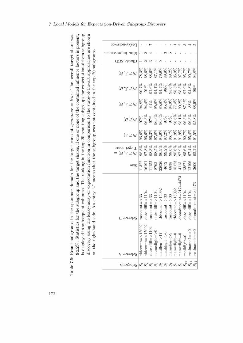
7 Local Models for Expectation-Driven Subgroup Discovery
Tab
le7.
5:R
esu
ltsu
bgr
oup
sin
the
spam
mer
dom
ain
for
the
targ
etco
nce
ptspammer
=tr
ue.
Th
eov
erall
targ
etsh
are
was
94.2
%.
Sta
tist
ics
for
the
sub
grou
pan
dth
eta
rget
shar
es,
ifon
eor
non
eof
the
conta
ined
infl
uen
cefa
ctors
isp
rese
nt,
isd
isp
laye
din
sub
sequ
ent
colu
mn
s.T
he
ran
kin
gin
the
top
20re
sult
ing
sub
grou
ps
for
exp
ecta
tion
-dri
ven
sub
gro
up
dis
cove
ryu
sin
gth
ele
aky-n
oisy
-or
exp
ecta
tion
fun
ctio
nin
com
par
ison
toth
est
ate-
of-t
he-
art
ap
pro
ach
esare
show
non
the
righ
t-h
and
sid
e.A
nen
try
“-”
mea
ns
that
the
sub
grou
pw
asn
otco
nta
ined
inth
eto
p20
sub
gro
up
s.
Subgroup
SelectorA
SelectorB
Size
P(T|A,B)=Targetshare
P(T|A)
P(T|B)
P(T|A,B)
P(T|A,B)
P(T|A,B)
ClassicSGD
Min.improvement
Leaky-noisy-or
S1
tld
cou
nt=>
1509
2ta
scou
nt=>
33
11322
98,8
%96,6
%97%
94,8
%90,7
%78
,3%
11
-S2
tld
cou
nt=>
1509
2d
ate
diff
=>
1104
16191
97,8
%96,6
%96,3
%94,4
%91%
68,6
%2
2-
S3
dat
ed
iff=>
1104
tasc
ount=>
33
11152
98,3
%96,3
%97%
94%
92,6
%88,6
%3
47
S4
nam
edig
it=>
0d
ate
diff
=>
1104
8763
98,5
%97,8
%96,3
%95,8
%94,7
%87,1
%4
--
S5
mai
llen
=>
17tl
dco
unt=>
15092
22026
96,9
%94,9
%96,6
%85,8
%94,4
%79,9
%5
--
S6
mai
ldig
it=>
0ta
scou
nt=>
33
4672
99,2
%97,2
%97%
95,4
%96%
89,9
%-
3-
S7
nam
elen
=>
9ta
scou
nt=>
33
6838
98,6
%96,7
%97%
94,9
%95,6
%89
,2%
-5
-S8
nam
edig
it=
0tl
dco
unt=>
15092
15173
95,6
%91,9
%96,6
%77,4
%98,3
%95,9
%-
-1
S9
nam
edig
it=
0d
omai
nco
unt=
2174-4
473
4115
97,9
%91,9
%98,1
%90,2
%98,5
%97,7
%-
-2
S10
mai
ldig
it=
0d
ate
diff
=>
1104
13871
95,6
%92,7
%96,3
%87,1
%97,9
%95,7
%-
-3
S11
real
nam
e2=>
0d
ate
diff
=>
1104
12196
97,4
%95,4
%96,3
%88%
94,8
%90
,7%
--
4S12
real
nam
elen
=0
dom
ain
cou
nt=>
4473
3600
95,2
%91,5
%95,8
%88,9
%96%
94,8
%-
-5
172

7.7 Evaluation
In contrast to these results, applying the leaky-noisy-or model leads to a completelydifferent set of results: The target shares in the result subgroups are comparatively loweron an absolute scale. However, they can not be explained as easily. Consider for examplethe subgroup S8, the top subgroup according to the leaky-noisy-or model. This subgroupdescribes users, who have no digits in their username (namedigits=0 ) and use an emailaddress from a frequently used top-level domain (tldcount>15092 ). For users with ausername without digits, the spammer rate is substantially decreased to 77.4%. In otherwords, the share of real users (non-spammers) is increased by about a factor of four.On the hand, the influence of the top-level domain on the spammer rate is moderate inthe overall dataset. However, for users with a no-digit username, the information on thetop-level domain is significantly more important: If both factors occur together, thenthe likelihood of a spammer is re-increased to 95.6%. The other top subgroups for theleaky-noisy-or expectation function show similar statistical properties.
Overall, it can be observed that the discovered subgroups differ significantly for theapplied measures. Both types of subgroups can be of interest for the users, dependingon the exact project goal. If the required type of subgroups is not clear beforehand, thena combination of results from novel and traditional approaches might be useful.
Expectation-driven subgroup discovery was also used to discover interesting subgroupswith a larger description, i.e., subgroup described by a conjunction of three selectors.One of the top subgroups discovered in this setting is described by (tasperpost=[0-1] ∧tascount=[6-11] ∧ date diff=[0-7]). The statistics of this subgroup and its generaliza-tions are displayed in Table 7.6.
Table 7.6: Statistics for an exemplary result subgroup of expectation-driven subgroupdiscovery that is described by a conjunction of three selectors.
Subgroup description Size Target share
tasperpost=[0-1]∧ tascount=[6-11]∧ date diff=[0-7] 30 86.7%tascount=[6-11]∧ date diff=[0-7] 123 54.5%tasperpost=[0-1]∧ date diff=[0-7] 110 38.2%tasperpost=[0-1]∧ tascount=[6-11] 188 81.9%date diff=[0-7] 899 53.5%tascount=[6-11] 5103 93.2%tasperpost=[0-1] 1588 79.5%All instances 31034 94.1%
All single influence factors of this subgroup either have little influence or a strongnegative influence on the target share. As could be expected, all combinations of twoof these influence factors lead to a strong decrease of the target share as well. However,if all three of these influence factors are combined, then the target share is increasedin comparison to all combinations of two of these factors. This potentially interest-ing subgroup is never discovered by the traditional methods since the target share of
173

7 Local Models for Expectation-Driven Subgroup Discovery
(tasperpost=’0-1’ ∧ tascount=’6-11’ ∧ date diff=’0-7’) is still lower than the target sharein the overall dataset. Nonetheless, this example also shows that the explanation, whya certain subgroup is considered as interesting gets more complex and more difficult tocomprehend for subgroups with longer descriptions. Therefore, the maximum numberof selectors in a subgroup description in these case studies were limited to two or three,dependent on the specific task.
In summary, the application of expectation-driven subgroup discovery using a localmodel enabled in both case studies the identification of interesting subgroups with a tar-get share that was higher than expected. Using traditional approaches, these subgroupsoften remained undetected.
7.8 Discussion and Possible Improvements
As shown in the previous sections, the mining for unexpected subgroups, e.g., by theleaky-noisy-or function finds qualitatively different subgroups than the traditional ap-proaches on subgroup discovery: Result subgroups potentially have a target share thatis not increased in comparison to all generalizations or the overall dataset, but are stillconsidered as interesting, if the single influence factors that compose the pattern implya stronger decrease. Such subgroups receive a negative score in subgroup mining withtraditional measures qKl(P ) or minimum improvement-based interestingness measuresqMI(P ). Thus, they will never be discovered using traditional measures, even if thenumber of presented subgroups is increased, e.g., to the best 100 subgroups. While suchsubgroups are certainly interesting in some applications, this depends on the specificgoal of the project and might not be the case in others.
If the required statistical properties of subgroups are uncertain, then a good solutioncan be, to combine the result subgroups for different interestingness measures. For thatpurpose, different approaches can be used. In the most simple case, the top subgroupsfor the different interestingness measures are compiled in a single list, e.g., by takingthe best five subgroups of each approach. Since the minimum improvement can also beapplied as an additional constraint, another solution could be, to use results for classicsubgroup discovery with an additional filter for (significant) minimum improvement andsupplement this list with additional results obtained from the leaky-noisy-or-model. Inboth cases, however, an overall ranking on the combined result subgroups is missing.Another combination approach generates such an overall ranking: The definition oninterestingness measures with expectation functions allows for a comfortable methodto combine results from different techniques directly in the search: For this purpose, anew (meta-)expectation function is created that combines expectation functions χ1 . . . χIwith user defined weights w1 . . . wI in a weighted sum:
χcomb(expi, wi, sg) =
∑Ii=1wi · χi(sg)∑I
i=1wi
174

7.9 Summary
Mining subgroups using such a combined expectation function takes all involved expec-tation functions into account. Additionally, weighting the different functions allows theuser to emphasize on the type of subgroups he is most interested in.
The target share expectation that a user forms on a specific subgroup is heavily influ-enced by the provided information. For the models in this work, i.e., the additive andmultiplicative synergies, the leaky-noisy-or model and the logit model, the knowledgeon the target share in presence of exactly one of the two influence factors is assumed,e.g., P (T |A, B). If instead other statistics are used for the subgroup introspection, e.g.,the target share for a generalization P (T |A), models could be adapted accordingly. Forexample, as a rough approximation the equality P (T |A, B) = P (T |A) could be used.
Furthermore, the proposed models, in particular the leaky-noisy-or, assume in theorythat the influence factors that are combined in a subgroup are conditionally independentfrom each other. They do not take the similarity of coverage of two factors into account.Therefore, the computed expectation for the target share might be off if two factorsare strongly dependent from each other: For example, assume that the influence factorX has a decreased target share in comparison to the overall dataset and the factor Yhas the same target share as the overall dataset. Based on this information, one wouldexpect that the target share in X ∧ Y is also decreased, since Y has seemingly no effecton the target share. This is also reflected by the computed expectation value from theleaky-noisy-or model. However, if it is additionally known that all instances covered byY are also covered by X, i.e., sg(Y ) ⊂ sg(X), then the user’s expectations change. Sincein this case the coverage of X ∧ Y is identical to the coverage of Y , the target shares inthese subgroups are also identical. In this situation, the target share of X ∧ Y is higherthan the expectation computed by leaky-noisy-or. As a consequence, the subgroupX ∧Y is a possible result if the leaky-noisy-or is applied to calculate expectation values.However, the subgroup is obviously not interesting considering the covering information.One possibility to avoid such findings is, to ignore subgroups, which show a very largeoverlap (e.g., more than 90%) with a generalization. This adaptation has already beenapplied in the case studies of Section 7.7.
Finally, the framework in its current form takes only the absolute differences betweenthe actual and the expected target share into account. However, a fixed increase of thetarget share is probably more important for very low or very high probabilities. Forexample, if the expected target share is at 50% then a difference of 3% to the actualtarget share of 53% is probably not that important. In contrast, a difference between95% and 98% target share is substantial. These considerations could be used to furtherimprove the proposed approach in future extensions.
7.9 Summary
This chapter introduced a novel family of interestingness measures in order to improvesubgroup discovery results. The novel measures incorporate the expectations of the sub-groups’ target shares. These are implied by the statistics for the influence factors that arecombined to describe the subgroup. To compute plausible values for these expectations,
175

7 Local Models for Expectation-Driven Subgroup Discovery
which are in line with human reasoning, techniques from research on bayesian networkscould be transfered to the subgroup discovery setting. In particular, it was proposed togenerate fragments of bayesian networks as local models. Based on these models severaltechniques were proposed for the calculation of expectation values. The advantages ofthe novel approach were demonstrated in several experiments, including two real-worldcase studies. In both domains the novel approach enabled the identification of interestingsubgroups that could not be detected using state-of-the-art algorithms. Advantages aswell as potential problems with the novel approach have been discussed. This providedalso some pointers to future improvements. Furthermore, the extension of the proposedframework in the direction of numeric target attributes and exceptional model mining aswell as the integration of background knowledge into the local models seem promising.
176

8 VIKAMINE 2: A Flexible Subgroup DiscoveryTool
Subgroup Discovery is not an isolated automatic process, but an iterative and interactivetask, see also Section 2.7. To support the user in this course of action, advanced toolsupport is required.
For this reason, already early subgroup discovery algorithms have been embeddedinto powerful tools that provide a graphical user interface as well as options to visu-alize the results. These pioneering systems include Explora [140], KEPLER [262] andSubgroupMiner [143, 144]. Nowadays, the most popular data mining tools cover a widevariety of data mining tasks, for example RapidMiner1, Knime2, Orange3 or Keel4. Theintegration of different data mining approaches in a single tool provides many benefits.However, the task of subgroup discovery is in these tools often only supported on a basiclevel with few discovery algorithms and visualization options. Often, subgroup discoveryis only available in these tools as a plugin.5 In addition, these multi-purpose tools arearguably more difficult to start with for practitioners. An open-source tool specializedon subgroup discovery is Cortana6. It provides an easy-to-use graphical user interface,multiple mining algorithms and options for result visualization. From an algorithmicpoint of view, Cortana places emphasis on heuristic search algorithms and exceptionalmodel mining.
VIKAMINE is an alternative, freely available data mining tool that is also special-ized on the task of subgroup discovery. In the context of this work, VIKAMINE wassubstantially improved and extended to the novel VIKAMINE 2. The improvementsinclude additional algorithms, interactive mining approaches, pre-processing techniques,methods for result presentation, and a novel user interface.
This chapter first provides a general overview of VIKAMINE 2. Then, some contribu-tions to VIKAMINE 2 that were developed in the context of this work are highlighted.Previously available functionality of VIKAMINE has been described in [20].
1www.rapidminer.com2www.knime.org3www.orange.biolab.si4www.keel.es5As an example, http://kt.ijs.si/petra kralj/SubgroupDiscovery/ provides plugins for Orange and
RapidMiner are available.6www.datamining.liacs.nl/cortana.html
177

8 VIKAMINE 2: A Flexible Subgroup Discovery Tool
8.1 VIKAMINE 2: Overview7
The VIKAMINE project has been started in 2003 by Martin Atzmueller. The soft-ware is implemented in Java and is freely available as open-source, licensed under theLesser General Public License (LGPL). VIKAMINE 2 is available for download atwww.vikamine.org. In collaboration with the original author, the tool was signif-icantly enhanced in the context of this work. The current features of VIKAMINE 2 in-clude:
� State-of-the-art algorithms for subgroup discovery: VIKAMINE 2 comeswith a variety of established and state-of-the-art algorithms for automatic subgroupdiscovery, e.g., beam search [167], BSD [177] or SD-Map [22, 24]. The algorithmicimprovements introduced in chapters 4, 5 and 6 have also been implemented forVIKAMINE 2, partially as plugins.
For the algorithms, the user can choose from a wide selection of interestingnessmeasures, e.g., weighted relative accuracy, the binomial measure, the χ2 measure,the lift, the t-score, the variance reduction and many more, see Section 2.5.3 for adescription of these measures. Results can be optimized by applying discretizationor filtering techniques that utilize relevancy or significance criteria.
� Visualizations and interactive mining: Powerful visualizations are essentialto achieve a quick understanding of the data and mined subgroups. Visualizationsimplemented in VIKAMINE 2 include, for example, pie visualizations, box visu-alizations, specialization graphs, and visualizations of subgroup statistics in theROC-space, see also Section 8.6. Furthermore, VIKAMINE 2 provides methodsfor the exploratory mining of subgroups, e.g., the zoomtable [25] or the dynamicsubgroup tree, see Section 8.5.
� Import/Export: Datasets can be imported from different file-formats, for exam-ple, from CSV files in different configurations or from the ARFF format of WEKA.Modified or filtered datasets can be exported in the same file formats. Connectionsto SQL databases are enabled by plugins. Results can then be exported as plaintext, to XML, or directly for presentation in standard Office Tools, e.g., MS-Excel.
� Background knowledge: VIKAMINE 2 supports various methods to integratebackground knowledge into the mining process, e.g., on default values or dis-cretization cutpoints. Background knowledge can be acquired using form-basedor document-based approaches, see also Section 8.7.
� Extensibility: Using the Rich Client Platform (RCP) of Eclipse, VIKAMINE 2can easily be extended by specialized plugins. Extension points allow, for example,
7This section contains contents previously published in [16]: Martin Atzmueller and Florian Lemmerich:VIKAMINE – Open-Source Subgroup Discovery, Pattern Mining, and Analytics. In Proceedings of theEuropean Conference on Machine Learning and Knowledge Discovery in Databases (ECML/PKDD),2012.
178

8.2 Architecture
for quick integration of new interestingness measures, search algorithms, visualiza-tions, types of background knowledge and specialized views on the data into thegraphical user interface.
� Modularity: VIKAMINE 2 utilizes a strict separation between kernel compo-nents, i.e., data representations and algorithms, and the graphical interface com-ponents. Thus, the algorithmic core functionalities of VIKAMINE 2 can be easilyintegrated in other systems and applications, e.g., for the integration in productionenvironments, or for evaluations of algorithms by researchers, see also the followingsection.
8.2 Architecture
Application scenarios for a subgroup discovery tool are diverse: It may be used for in-teractive subgroup discovery by domain experts, for the regular automatic generationof documents as reports, or as a library to determine result subgroups, which are usedas input for other machine learning or data mining algorithms. Many of these applica-tions do not require the heavy-weight components used for graphical user interfaces orthe generation of office documents, e.g., spreadsheets. To reduce the overhead in suchapplications, VIKAMINE 2 pursues a strict separation of components:
� Vikamine Kernel: The kernel is the core of the software. It provides functionalityfor loading, storing and handling the dataset, and for mining subgroup patterns.It contains a wide collection of efficient subgroup discovery algorithms and inter-estingness measures as well as methods for filtering results. Mining tasks can bedescribed using Java code or using a declarative XML specification.
� Vikamine Office: This is a minor addition to the kernel functionality that allowsexporting subgroup discovery results in MS-Excel/LibreOffice Calc compatible fileformats and to generate overview reports.
� Vikamine RCP: This component provides a visual interactive user interface for au-tomatic and interactive subgroup discovery. It is described in more detail in Sec-tion 8.3.
� Vikamine Plugins: Plugins extend VIKAMINE 2 with additional functionality.These include novel algorithms, interfaces for interactive mining, reports, addi-tional handling of background knowledge and visualization options. Thanks tothe used RCP-environment GUI components are integrated seamlessly into theexisting interface.
8.3 An Extensible User Interface
The original VIKAMINE featured a Swing/AWT -based user interface. In the contextof this work, this was replaced by an interface based on the Eclipse rich client platform
179

8 VIKAMINE 2: A Flexible Subgroup Discovery Tool
(RCP). This framework provides an appealing, industry-proven robust and extensibleinterface environment. Information is organized in views and perspectives, which can befreely rearranged by the users.
A screenshot showing some fundamental views of VIKAMINE 2 is depicted in Fig-ure 8.1: In the workbench explorer on the left-hand side the source files for differentprojects can be organized, e.g., datasets, text files providing background knowledge orstored options from previous mining sessions. In the top middle, the currently selectedsubgroup and its statistics are displayed. At its right-hand side, the subgroup workspaceshows the results of the last discovery algorithm run or a set of user-selected subgroups.Below, the zoomtable allows for interactive mining of subgroups. On the right-hand side,the attribute navigator organizes the attributes of the dataset. It provides a variety ofoptions in the context menu, e.g., the discretization of attributes or modifying the cur-rently selected subgroup. Additional, more specific views are in the background or canbe added from the menu. Several commands, e.g., for running an automatic discoverytask, are accessible from the toolbar at the top.
Figure 8.1: A screenshot with some fundamental views of VIKAMINE 2 : On the left-hand side, the workbench explorer for project organization is shown. Atthe top, left of the middle statistics for the currently selected subgroup aredisplayed. Right of that, a set of result subgroups is displayed. At thebottom, the zoomtable view allows for interactive mining. On the right-hand side, the attribute navigator organizes the attributes of the dataset.Additional views can be opened, e.g., from the menu.
For data mining tools, extensibility is especially important since specific applicationprojects often require tailored algorithms, interestingness measures or visualizations, cf.also [262]. As a key functionality, the RCP-based architecture of VIKAMINE 2 allowsfor the simple development of extensions. These are created as (mostly) independent
180

8.4 Handling of Numeric Attributes
plug-ins and are seamlessly integrated in the user interface without modifying the basesource code. This is accomplished by implementing so called extension points. Forexample, VIKAMINE 2 provides extension points for the quick integration of novel
� subgroup discovery algorithms,
� interestingness measures,
� visualization components,
� acquisition and handling of background knowledge, and
� additional views, e.g., for interactive exploration.
The plugin architecture is in particular important for a tool heavily used in researchand education: It allows maintaining a small, but clean code base for fundamentalcomponents, but also enables integrated prototypes of experimental extensions.
8.4 Handling of Numeric Attributes
The original VIKAMINE had an emphasis on the nominal attributes in a dataset.VIKAMINE 2 provides improved support for subgroup discovery with numeric attributesin different areas:
Numeric target concepts are now available for automatic and interactive subgroupdiscovery. For automatic discovery, a variety of algorithms are available, including theSD-Map* and NumBSD algorithms presented in Chapter 4. To present subgroups withnumeric targets appropriately, presentation methods have been adapted accordingly, e.g.,the subgroup workspace or the visualization of patterns in PN-space (coverage space).
Numeric attributes can also be incorporated in the description of subgroups. Thenecessary discretization is performed either by manual elicitation using text-based orform-based knowledge acquisition, by automatic discretization, or by an interactive com-bination of both. Figure 8.2 shows the dialog that allows the interactive discretizationof attributes with respect to the chosen target concept for subgroup discovery. On thetop left-hand side an automatic discretization method can be selected, e.g., equal-width,equal-frequency, entropy-based, or chi-merge discretization, see Section 2.3.2. The tablebelow allows manual refinement of the results of the automatic step. On the right-handside, the distribution of the instances with respect to the current discretization is shown.The grey parts of the bars indicate the share of instances with a positive target con-cept. The name of the discretized attribute to be created is given at the bottom of theright-hand side.
8.5 A Scalable View for Interactive Mining
The interactive discovery of subgroups is a key application of VIKAMINE. However,previously proposed and implemented methods, e.g., the zoomtable or the tuning ta-ble [20], are severely limited in the number of involved attributes. To make interactive
181

8 VIKAMINE 2: A Flexible Subgroup Discovery Tool
Figure 8.2: The discretization dialog in VIKAMINE 2 : On the top left-hand side auto-matic discretization is performed. Below, the results can be manually refined.On the right-hand side the distribution of the instances with respect to thecurrent discretization is shown. Grey parts in the bars indicate the share ofinstances with a positive target concept.
mining available for large datasets with many attributes, the dynamic subgroup tree hasbeen developed as a combination of automatic and manual subgroup discovery. It isimplemented as a VIKAMINE 2 plugin.
In this view, each line of a table provides detailed statistical information on one sub-group. The initially shown subgroups are selected from the subgroups described bya single selector with respect to their score by a user chosen interestingness measure.Clicking on a subgroup dynamically expands the tree by computing and displaying thebest direct specializations of this subgroup. More subgroups with the same generaliza-tion can be shown on demand. An example of a dynamic subgroup tree is displayedin Figure 8.3.
This view follows an intermediate approach between automatic and manual discovery:An automatic component identifies potentially interesting candidate subgroups at eachlevel, while the user can guide the search by selecting for which candidates specializationsare investigated, cf. also [75]. Computations for specializations are only computed ondemand, i.e., if the user chooses to inspect specializations of the respective subgroup. Indoing so, interactive discovery can also be performed in large datasets with hundreds ofattributes. To improve scalability for large numbers of instances, interesting subgroupsand their statistics are computed on samples of the dataset first. As soon as more preciseinformation is available, the view is automatically updated.
182

8.6 Result Presentation
Figure 8.3: The dynamic subgroup tree plugin in VIKAMINE 2. Each line providesstatistics of a subgroup. Clicking on a subgroup dynamically expands thetree by computing the best direct specializations according to a chosen in-terestingness measure. More specializations can be shown on demand byclicking on the “Show more...” node in the tree.
8.6 Result Presentation
Efficient communication of the result to the end-users is a crucial step in data min-ing. This is in particular important for descriptive techniques like subgroup dis-covery, cf. [91, 258]. The visualization of subgroups has always been a focus ofthe VIKAMINE system. Currently implemented visualizations include specialization-graphs, representations in ROC-space and PN-space, pie visualizations, stacked bar visu-alization, box visualizations, and clustering-based overlap visualizations, see Figure 8.4for some examples. For a more detailed description of these implementations, we re-fer to [20, 14]. An overview on visualization techniques for subgroup discovery is alsoprovided in [158], see also [93].
This section introduces two novel presentation methods for subgroup discovery results:The pie circle visualization and the subgroup treetable. These are in particular motivatedby the intuition that subgroups with a conjunctive description should always be assessedwith respect to their generalizations, see also Chapters 6 and 7.
183

8 VIKAMINE 2: A Flexible Subgroup Discovery Tool
Figure 8.4: Exemplary visualizations in VIKAMINE : representations in ROC-space andPN-space, a specializations graph, pie visualizations, box visualizations, andclustering-based overlap visualizations.
8.6.1 Pie Circle Visualization
The pie circle visualization provides a quick overview on the most important influenceson a target concept. It is constructed as a graph of nodes and edges. The nodes of thegraph are laid out in a large circle in order to minimize overlaps between the edges. Anexample of this visualization illustrating the dropout rate in an educational domain canbe seen in Figure 8.5.
A single influence factor (subgroup) is represented by a node that is rendered as asmall pie chart, similar to [91]. The size of the subgroup is visualized by the node size:Larger nodes represent subgroups with a high instance count, smaller nodes representsubgroups that cover only few instances. The share of the target concept is displayedby the share of the filled part in the pie chart. For comparison, the target share for theoverall dataset is indicated by a narrow black line in the pie chart. Additionally, thedeviation of the target share in comparison to the overall dataset can be observed by thenode color. That is, nodes are displayed in red color, if the target share of the respectivesubgroup is higher than in the overall dataset, in green color, if it is lower (or equal).
In automatic discovery algorithms, subgroups are scored by an interestingness mea-sure. Such a measure can also be used to highlight the supposedly most interestingsubgroups in the visualization: Nodes with a high score are displayed with full color,less intense/lighter colors are used for subgroups with low scores. In doing so, the initialview on the visualization is more focused on the most important subgroups, while less
184

8.6 Result Presentation
Figure 8.5: An example of a pie circle visualization in the education domain. As targetconcept dropout = true was used. A single influence factor is represented bya node. The size of the subgroup is visualized by the node size. The share ofthe target concept is displayed by the share of the filled part in the pie chart.Additionally, the deviation of the target share in comparison to the overalldataset can be observed by the node color. Edges provide information onthe deviation of the target share for subgroups described by combinations ofinfluence factors.
important ones are displayed unobtrusive.
For example, consider the node foreigner=true at the left of Figure 8.5. The color ofthis node is red since the chosen target concept – dropout=true – occurs more often in thesubgroup described by this selector than in the total population. The filled part of thisnode indicates that for almost three quarters of this subgroup the target concept is true,while this is the case for only less than half in the total population as referenced by theblack line. The used interestingness measure relative added value, that is, the minimumdeviation of the target share with respect to generalizations of the subgroup, considersthe node as important. Therefore, the intensity of the red color is high. However, thenumber of instances for this subgroup is quite low, which is indicated by the small size
185

8 VIKAMINE 2: A Flexible Subgroup Discovery Tool
of the node.
If a combination of influence factors shows an interesting deviation of the target share,this is indicated by an edge between these nodes: Red colors signal a target share thatis higher than expected given the statistics of the incident nodes, green colors indicatea lower than expected target share. For possibilities to generate plausible expectationvalues for the target share of subgroups given the statistics of its generalizations, werefer to Chapter 7. As for the nodes, a high color intensity implies a high interestingnessscore using the chosen interestingness measure. Additionally, for important subgroupsthe edge width is slightly increased for emphasis.
For example, consider the edge between the nodes foreigner=true and degree=master.The red color of this edge implies that the subgroup foreigner=true ∧ degree=masterhas a higher target share than expected given the target shares for each of the two moregeneral subgroups. The applied interestingness measure indicates that this subgroup isof limited importance, the color intensity is low to medium.
The pie circle visualization is originally designed to present subgroups with at mosttwo selectors. Nonetheless, by adding nodes for subgroups with larger descriptions, alsomore complex subgroups can be represented. In this visualization, a larger number ofdisplayed subgroups requires a smaller node sizes to avoid overlap. However, as shownin the example up to 30 influence factors can be clearly presented, far more than byother visualizations that illustrate relations between subgroups, e.g., by a specializationgraph. Exact statistics for the influence factors and their combinations are available viaa tooltip. Of course, colors can be adapted for color blind users.
8.6.2 Subgroup Treetable
The subgroup treetable allows the interactive exploration of large result sets with standardoffice software, i.e., MS-Excel or LibreOffice Calc. In doing so, interactive mining canbe performed by domain experts without additional tools or potentially unsecure onlineaccess to the data. For that purpose, data mining experts generate the interactive reportwith VIKAMINE 2 and then send it to the domain experts. This report documentcontains a large set of candidate subgroups, e.g., by combining the results of differentdiscovery algorithm runs. These subgroups and all their generalizations are arranged ina tree like structure in the document. Children in the trees are initially hidden by the“group and outline” functionality of the spreadsheets and are only shown on demand.This follows the idea of the Information Seeking Mantra [225]: First provide an overview,then zoom in and provide details on demand.
For each subgroup, different statistics are displayed, e.g., the number of covered in-stances, the target share in the subgroup, and the statistical significance of the deviation.Since subgroups with longer descriptions appear multiple times in the tree, the size ofthe tree grows fast. This can be avoided by filtering out repeated appearances of asubgroup, if the deviation of the target share is low in comparison to the subgroup ofthe parent node.
An example of a subgroup treetable in MS-Excel is provided in Figure 8.6. The firstcolumn shows the description of the subgroup. The next columns present the subgroup
186

8.7 A Framework for Textual Acquisition of Background Knowledge
Figure 8.6: A screenshot of a subgroup treetable presentation in MS-Excel. Each rowpresents statistics for one subgroup, e.g., the number of covered instances, thetarget share in the subgroup, the statistical significance of the target sharedeviation in comparison to the overall dataset and the statistical significancewith respect to the generalization in the parent node. The signs – and + onthe left can be used to hide and show branches of the tree.
size, the target share within the subgroup and the statistical significance with respectto the overall dataset using a chi-squared test. The rightmost column indicates therelative significance, that is, the significance using the parent subgroup in the tree as thetotal population for the statistical test. Colors indicate strong deviations in the targetshare with respect to the parent nodes. Branches of the tree can be shown or hidden inMS-Excel using the markings + and - on the left side.
The structure of the tree resembles the dynamic subgroup tree, see Section 8.5. How-ever, in contrast to this view only pre-computed results are displayed. Since full subgroupdiscovery with higher search depths must be performed to generate the report, the cre-ation process takes more time than the refinement steps in the dynamic subgroup tree.However, the pattern treetable report enables (limited) exploratory mining of subgroupsfor domain experts, who only use standard office tools.
8.7 A Framework for Textual Acquisition of Background Knowledge
Integrating background knowledge in the mining process is important for efficientmining, see also Section 2.6. It is often limited by the knowledge acquisition bottle-neck [114, 113, 90], the problem of eliciting required knowledge from domain experts. Inthe previous versions of VIKAMINE, knowledge was acquired and used in separated di-alogs that directly initiated actions. In research on knowledge acquisition, the paradigmof document-centered knowledge acquisition has been proposed as an alternative to thisform-based approach: Users type their knowledge in a text document in an intuitive,easy-to-learn syntax. These are then processed by appropriate parsers to extract the
187

8 VIKAMINE 2: A Flexible Subgroup Discovery Tool
formal knowledge. This approach provides a variety of advantages, including low entrybarriers, example-based authoring and versioning support [215].
In addition to the form-based approach, VIKAMINE 2 also supports document-basedknowledge acquisition using a predefined syntax: Source documents containing knowl-edge can be edited within the program using the integrated text editor. If documentsin the respective folder of a mining project are created or edited, they are automati-cally parsed. The extracted, formalized knowledge is then saved in a central reactiveknowledge store in the form of triples similar to a RDF-Triple, e.g., <AttributeX; has-DefaultValue; none>. The reactive knowledge store manages a set of triggers, whichinitiate actions if certain types of knowledge are inserted to the store. For example,a new attribute is created if a novel discretization scheme for a numeric attribute isprovided. Additionally, interface views or mining algorithms can query the store forknowledge. The set of parsers to extract knowledge from the documents and the trig-gers for the knowledge can be easily expanded using extension points in order to adaptto project specific requirements. This course of action is also illustrated in Figure 8.7.
Figure 8.7: The main course of action knowledge handling in VIKAMINE 2 : The usercan insert knowledge using forms (dialogs) or using text documents writtenin an intuitive syntax. These documents are parsed and the extracted knowl-edge is stored in a central reactive knowledge store. This store manages a setof triggers. These are activated, if a specific type of knowledge is changed,and initiate respective actions. Additionally, the store can be queried fromdiscovery algorithms or views for interactive mining.
The following simple examples of text fragments illustrate how some important typesof knowledge can be formalized and used. However, the power of the approach lies notin these specific use cases, but in its easy extensibility with respect to novel knowledgetypes and actions, which allows adapting to the problem at hand quickly.
� Default values: Knowledge on default values can for example be used to ignorethe respective attribute values in subgroup discovery algorithms.
DEFAULT of previous_degree_program: false
� Discretization: This provides a natural segmentation of the domain of a numericattribute. When knowledge of this type is inserted to the reactive store, then atrigger is activated to create a new discretized attribute.
188

8.8 Integrated Exploratory Data Analysis with EDAT
DISCRETIZATION of starting_age: [18;20;25;30]
� Abnormality information: Similar to discretization information, entering thisknowledge creates a new attribute with values low, normal, and high. This kind ofbackground knowledge is in particular common in medical domains.
NORMAL of blood_pressure: 90-120
� Value categorization: This creates a new attribute that summarizes values ofthe original attribute. In the following example, the dataset contains an attributecourse program with the values physics, chemistry, biology, history, law, literatureand some other values. The provided knowledge implies the creation of a newattribute faculty with three values: other, science and humanities, which are setin the instances according to the value of the attribute course program.
CATEGORIZATION of course_program: faculty, DEFAULT other- science-- physics-- chemistry-- biology- humanities-- history-- law-- literature
� Ordinality: This type of knowledge provides an ordering for the values of an at-tribute. This can be used, for example, to generate selectors such as highest degree≥ master.
ORDINALITY of highest_degree: none < bachelor < master < phd
As shown by these examples, textual knowledge acquisition methods enable the intu-itive elicitation of background knowledge, which can be used for more effective subgroupdiscovery.
8.8 Integrated Exploratory Data Analysis with EDAT
A pre-requisite for effective subgroup discovery is that users are familiar with the maincharacteristics of the analyzed data. For this task, exploratory data analysis [238, 118]has been developed in the field of statistics. This approach analyzes the distribution ofa dataset by providing the user a large variety of visualization methods, e.g., pie charts,bar charts, histograms, mosaic plots, scatter plots and many more. A similar set oftechniques is required for subgroup introspection, that is, the examination of potentiallyinteresting subgroup patterns. Thus, techniques from exploratory data analysis do not
189

8 VIKAMINE 2: A Flexible Subgroup Discovery Tool
only allow obtaining an overview of the analyzed data. By visualizing distributions anddependencies in the subgroup as well as in the overall data, they also allow assessingand possibly explaining deviations of the target concept in the subgroup.
The Exploratory Data Analysis Tool (EDAT) was developed as a plugin to makemethods for exploratory data analysis accessible in VIKAMINE 2, see also [187]. Itcan use exploratory techniques implemented in Java, but also functions as a bridgebetween the Java-based VIKAMINE 2 environment and the statistical programminglanguage R8 [212]. For R a wide variety of statistical and graphical implementationsare freely available, either in the core installation or in one of almost 5000 extensionpackages. However, R is primarily designed as a programming language for experiencedusers, who write code in a console. EDAT provides an intuitive graphical user interfacefor visualizations implemented in R to make these accessible to laymen. It offers apredefined, but extensible set of these visualizations directly integrated in VIKAMINE 2 .Thus, datasets as well as subgroups can be easily inspected using one of many availablevisualization techniques implemented in R.
Figure 8.8 shows an exemplary screenshot of the EDAT plugin: In the top left viewone of the available analysis methods is selected. Depending on the chosen evaluation,parameters can be specified below, e.g., which attributes are visualized. In the center ofthe screen, the result of the last command is displayed, in this example a density plot.Results can be exported as graphics or internally stored for later use in the history view,which is shown at the bottom of the screen. The view on the right-hand side providesadditional information, e.g., the available attributes or the R code of the last generatedevaluation. For users familiar with the R language, code can also directly be entered ina console (in this screenshot only in the background).
The available evaluation techniques presented in the user interface can easily be ex-tended: Declarative XML-files specify the name, category and parameters of an evalua-tion as well as the (Java or R) code templates, which are to be executed to generate theresult. Overall, the exploratory data analysis tool EDAT provides many visualizationtechniques to inspect the distribution of a dataset or a specific subgroup by integratingimplementations written in R into the VIKAMINE 2 user interface.
8.9 Summary
The subgroup discovery tool VIKAMINE was substantially improved and extended inthe context of this work: VIKAMINE 2 provides a broad collection of state-of-the-artalgorithms and interestingness measures for mining with binary as well as numeric targetconcepts, including the novel algorithms presented in the previous chapters. A newgraphical user interface based on the Eclipse RCP framework enables easy extensibility.In addition, new options for interactive mining and result presentation were developed,e.g., the dynamic subgroup tree, the pie circle visualization and the subgroup treetable.Furthermore, the plugin EDAT adds a large range of visualization options for inspecting
8www.r-project.org
190

8.9 Summary
Figure 8.8: The EDAT perspective in VIKAMINE 2. In the top left view, the userchooses a visualization. Below parameters for this visualization can be se-lected. The central view shows the last executed query. In the bottommiddle, the history of results is displayed. The view on the right-hand sideprovides additional information.
the distribution in the overall dataset as well as in specific subgroups by providing abridge to the programming language R.
191


9 Applications: Case Studies in SubgroupDiscovery
This chapter presents several case studies that were performed in the context of this work.They exemplify how subgroup discovery can successfully be applied in real-world sce-narios using the developed methods and algorithms. First, an ongoing long term projectregarding the analysis of educational data from the university domain is introduced.In this context, it is described, how subgroup discovery can reveal influence factors onthe success and the satisfaction of students. Furthermore, an extended case study con-cerning the mining of social web data is provided, which aimed at describing locationsusing the tags that users provided for geo-referenced images. Additionally, the chapteroutlines further applications of supervised pattern mining that were approached in thecontext of this work. These are concerned with the improvement of graphical modelsfor information extraction, an evaluation of the case-based training system CaseTrain,the identification of influences that lead to faulty products in an industrial domain, andwith the IPAT pattern mining challenge.
9.1 Students’ Success and Satisfaction
Monitoring the curricula of university students provides great benefits for faculty staff:It allows for example to identify changes in enrollments, delayed graduations, difficultcourses, and individual students in danger of dropout. By keeping these factors undersurveillance, an early-alarm-system can be implemented in order to take appropriateactions in time or to evaluate the effects of applied changes.
The project StudiPro implements such a monitoring system for the University ofWurzburg. It regularly generates a variety of compact reports, which present sum-marized information on different levels: For degree programs key numbers include theoverall number of students, beginners, dropouts, graduations, female students, foreignersand several other statistics. On course level, the average grade, the rate of failed examsand the rate of exams passed too late in the curriculum are key statistics to identify crit-ical teaching modules. Beside these key reports, further reports provide more detailedinformation on demand. Several of these tasks employ subgroup discovery as a datamining technique. These applications are described in the next sections in more detail.
Several concrete actions were at least partially motivated and/or monitored by thisproject: For example, individual students in danger of dropout have been invited toa discussion with a mentor. As another example, a previously joint course for severaldegree programs was split since it turned out to be too difficult for a part of the students.
193

9 Applications: Case Studies in Subgroup Discovery
The created statistics are currently also a required part of the yearly reports of thefaculties to the heads of the university for quality control in the degree programs.
9.1.1 Dropout Analysis1
A first analysis focuses on influence factors, which lead to the dropout of students, that is,the abandonment of degree programs without graduation. Dropouts often occur earlyin the degree programs, that is, in the first two semesters of the studies. Therefore,indicators should not be based on exam results of the students, but on information,which is already known at the beginning of the study. For that purpose, datasets aregenerated that include information on the place, type and grade of the school final exam,previous courses and degree programs on this university, and personal information suchas gender and age. As target concept, the overall success of the studies was used, that is,dropout or graduation for the degree program. Separate analyses in that direction aregenerated and reported regularly in an automatic way, but these are limited to simplesubgroup descriptions without conjunctions, see Figure 9.1. In addition, more detailedanalysis reports are created on demand. These also contain interesting combinationsof subgroups and can cover a wide range of different degree programs for more generalfindings.
However, the starting point for any more elaborated subgroup discovery was alwaysgiven by an overview on the basic influence factors, either in a separate report as depictedin Figure 9.1, or in the respective view in VIKAMINE 2. This was also the case in thesubsequent applications, even if it is not explicitly mentioned. Exceptions are only casestudies, which already have a very large number of single influence factors, such as insocial media case study, see Section 9.2.
One exemplary, interesting finding was that the school final exam grade is stronglycorrelated with the success of the university degree programs. This correlation is in linewith educational research on this topic, cf. [83]. In this direction, an interesting detailcould be observed for several degree programs: In general the dropout ratio is lower,the better the school final exam grade was. However, this is not the case for studentswith very good school grades. These drop out slightly more often then their colleagueswith good, but not very good grades. For example, in a certain degree program, whichis also analyzed in Section 9.1.2, the overall dropout rate of the 708 analyzed studentswas 30.9%. The 124 Students with a school final exam grade between 2 and 2.5 (1 isbest) dropped out in only 12.9% of cases. However, for the subgroup of 71 students withthe best final school grades (better than 2) the decrease was not as strong since theydropped out only in 25.4% of the cases, see also Figure 9.1.
Additional results for the analysis of student dropouts, which also cover combinationsof influence factors, have already been presented and discussed in depth in the contextof expectation-driven subgroup discovery, see Section 7.7.3 of this work.
1Some contents of this section have been published as [175]: Florian Lemmerich, Marian Ifland, andFrank Puppe: Identifying Influence Factors on Students Success by Subgroup Discovery, In Proceed-ings of the 4th International Conference on Educational Data Mining (EDM), 2011.
194

9.1 Students’ Success and Satisfaction
Figure 9.1: Example of a basic report on student dropouts for one degree program ina spreadsheet (translated). Colored rows highlight influence factor with astrong deviation of the target concept dropout.
9.1.2 Indicators for Thesis Grades
A similar dataset as for the dropout analysis can also be used for other target conceptsthat measure student success. For that purpose, respective attributes are added to thedataset, e.g., the final grade of the degree, the number of semesters until graduation, thecontinuation of studies in a master degree after graduation, or the grade of the (bacheloror master) thesis. Since these statistics are measured at the end of studies, they canalso be related to student performances within the degree program, e.g., the averagegrade or the number of ECTS credits acquired in certain time frames. If the analysisfocuses on a single degree program, then additionally grades and semesters for specificrequired courses can be used. In the following, some results for an exemplary analysisare outlined, which was concerned with influence factors on the final thesis grade of acertain established degree program:
195

9 Applications: Case Studies in Subgroup Discovery
Table 9.1: Some exemplary results for influence factors on the thesis grade (1 is bestgrade).
Description # Stud. Avg. thesis grade
Overall 489 2.18Grade course A > 3.5 109 2.52Grade course B > 3.5 83 2.51Avg. grade all required courses > 3.5 14 2.46Avg. grade all required courses > 3.0 286 2.42Grade course A > 3.5 AND Grade course B > 3.5 24 2.98Grade course C < 1.5 AND Avg. grade non-req. < 1.5 21 1.56Grade course C < 1.5 98 1.99Avg. grade non-req.< 1.5 70 1.93
The average thesis grade in this degree program was a 2.18. Regarding single influencefactors, subgroup discovery identified in particular two required courses, whose gradesare indicators for weaker thesis grades. For students with a bad grade (> 3.5) at thesemodules, the average thesis grade was significantly worse than 2.18, that is, 2.52 and2.51 respectively. Having a bad grade at these modules had an even stronger impact onthe thesis grade than the average grade of all required courses, which was at about 2.4.
To find candidates for interesting combinations of influence factors, subgroup discoverywith minimum improvement interestingness measures was applied. Since it was focusedon subgroups with a large deviation of the target concept, the size parameter was set toa low value of a = 0.1. Interestingly, a search depth of three returned the same resultsas a search with a depth of two, indicating that no combinations of three describingselectors were considered as interesting by the chosen interestingness measure.
The most prominent finding was that if both of the previously identified critical mod-ules were completed with a bad grade, then the average thesis grade was disproportion-ately worse, as it deteriorated to 2.98. A possible explanation for this phenomenon isthat both courses are from quite diverse subfields of the degree program. If studentshave bad grades in different areas, then they will also have to choose a thesis topicfrom such a subfield. Another interesting finding was a subgroup that described studentwith a good grade in another, math-related course and also good average grades in thenon-required courses. For these, the thesis grade was also very good on average, eventhough the results for these factors were less decisive on their own: If grades in bothareas were good, then the average grade was 1.56. The respective value for the singleinfluence factors were 1.99 and 1.93 respectively, see also Table 9.1.
In this scenario, the interactive nature of subgroup discovery was evident. While au-tomatic subgroup discovery with minimum improvement measures generated interestinghypotheses, these were always compared manually to subgroups with related and “moregeneral” descriptions. Here, however, the term “general” does not only refer to the strict
196

9.1 Students’ Success and Satisfaction
formal definition, but also to background knowledge: The average grade of all requiredcourses is perceived as “more general” than the grade of a single module. For this task,the interactive GUI of VIKAMINE 2 proved to be an essential support tool to comparesubgroup statistics quickly. For the future, an extension of expectation-driven interest-ingness measures for numeric target concepts could be helpful to find further interestingsubgroup patterns.
9.1.3 A Survey Analysis on Student Satisfaction
In another sub-project of StudiPro we conducted a large voluntary online survey, whichwas directed at all students of the University of Wurzburg. Beside generating overviewstatistics for this survey, subgroup discovery was applied for a deeper analysis.
9.1.3.1 Dataset
The key question of the survey was how satisfied students are with their studies overall.Additional questions asked the students, which degree programs they study, how farthey have progressed in their studies, how fit they feel for the requirements of theirprogram, how well they feel informed about their situation, how much time they spendon studies and at additional jobs to earn their living, and which organizational issuesaffect their studies. Subjective impressions, e.g., about their satisfaction or currentstate of information, were given on a scale from 1 to 6, matching the German schoolgrading system. Since one student can be enrolled in more than one degree program,one boolean attribute was used for each degree program. Additionally, degree programswere summarized by their field (e.g., science, humanities, economics,...) and the kindof degree (e.g., bachelor, master, state examination, ...). Thus, the overall datasetcontained 119 attributes. To not decrease the response rate of the survey by privacyconcerns, it was made completely anonymous. Therefore, it could not be linked to thestudents exam data. Overall, about 2800 student participated at the survey.
9.1.3.2 Influence Factors for the Overall Satisfaction
The main questions of this survey were concerned with the overall satisfaction of thestudents and which factors do influence this rating. For this task, subgroup discoverywas applied with the attribute satisfaction as the numeric target concept. The meantarget value using this attribute was at 2.61 (on a scale from 1-6, where lower numbersindicate higher satisfaction), showing an overall high satisfaction with the universityexperience. Numeric describing attributes were discretized manually to achieve moreexpressive values. Regarding the attributes for degree programs, only selectors werecreated, which refer to a true value of the attribute. That is, the search space containedno selectors that indicate that a student is not studying a certain subject.
As selection criteria, standard mean-based interestingness measures as well as generali-zation-aware measure using the minimum improvement were tested. Using a trivialsearch algorithm with a maximum search depth of 5, an exemplary task took up to onehour to compute. By utilizing a bitset-based data structure and the improved pruning
197

9 Applications: Case Studies in Subgroup Discovery
bounds presented in Chapters 4 and 6, the runtime could be substantially decreased: Thesame task took about 20 seconds using a bitset-based data structure without optimisticestimate pruning and only two seconds using the full NumBSD algorithm. Althoughsubgroup discovery could also be performed with less sophisticated methods in this con-text, the improved algorithmic efficiency allowed to comfortably explore a large varietyof different interestingness measures.
Result subgroups from the classic mean-based interestingness measures had higherabsolute deviations of the target concept. However, they also had longer, more difficultto interpret descriptions and were often highly redundant to each other. For example,for a search depth of 2, 14 of the top 20 subgroups that indicate a decrease of thesatisfaction were specializations of one single influence factor. In contrast, the resultsfor generalization-aware measures offered a larger variety of subgroups that had shorter,simpler descriptions. Therefore, these results were overall more useful for the goal of iden-tifying understandable influence factors. Since in this particular task higher deviationswere considered as more important than large coverage, relatively low values for the sizeparameter a provided the (subjectively) best results. The exemplary results describednext have all been discovered using a generalization-aware interestingness measure withthe parameter a = 0.3. They are summarized in Table 9.2.
Table 9.2: Exemplary results for the survey analysis. These subgroups show an interest-ing deviation from the overall satisfaction level in the survey. The satisfac-tion was provided on a scale from 1 to 6, 1 being the rating for the highestsatisfaction.
Description # Students Mean satisfaction
Overall 2799 2.61Matching requirem. = [4-6] 258 3.46Matching requirem. = [4-6] ∧ Information = [4-6] 55 3.93Overcrowded courses = true 887 2.89Overlapping courses = true 1030 2.85Degree program = Medicine 321 2.24Degree program = Medicine ∧ Semester= [1-2] 70 1.93
The overall satisfaction correlates strongly with how students feel up to their studies:Students, who do not feel to match the requirements (with a grade of 4 or worse on ascale from 1-6) have an overall satisfaction with their studies of 3.46, compared to the2.61 in the total population. However, this is the case for less than 10% of the sur-vey participants. The satisfaction decreased further if the students felt additionally notwell informed about their situation. For the respective students the average satisfactiondropped to 3.93. Organizational issues also played a role for student satisfaction: Stu-dents, which were affected by overcrowded or overlapping courses, also were less satisfiedwith their studies overall, showing a rating of 2.89 and 2.85 respectively. As the high
198

9.1 Students’ Success and Satisfaction
number of concerned students indicates, these are perceived as wide spread problems atthis university.
Regarding degree programs, some subjects had especially satisfied students: For ex-ample, students aiming at a medical degree had an average satisfaction rating of 2.24.In particular, students in the first semesters of this degree program were satisfied. Theyshowed an average rating of 2.05.
Overall, subgroup discovery showed to be an effective tool for identifying influencefactors in this setting. Subgroups with short descriptions were more useful for thistask, as it was aimed at identifying general influences for student satisfaction. Formalstatistical significance of the discovered subgroups in this setting was considered as notrelevant in this context, as the voluntary participation in the survey already implies abias. Although some of the findings could be expected beforehand, the comparison of theimpact of different factors lead to interesting insights. Some of the previously assumedfactors turned out to have little influence on satisfaction, e.g., the time required for thestudies in semester breaks. While such findings could not be discovered using automaticdiscovery, they could easily be checked using the interactive VIKAMINE 2 tool.
9.1.3.3 Gender Diversity in Student Satisfaction
Diversity, in particular gender diversity, has become an important topic in education inthe last years. The overall survey results suggest that there is only a marginal differencein the overall student satisfaction between male and female students: Male studentsprovided a mean satisfaction score of 2.56, while the mean score for females was 2.62.However, there may be certain conditions, which cause the satisfaction to differ betweengenders. To identify these conditions, we applied a variant of exceptional model mining.Classic subgroup discovery cannot be applied in this setting, since the target concept in-volves two attributes, the binary attribute gender and the numeric attribute satisfactionrating. As this problem setting is to the author’s knowledge not covered by previouslyproposed model classes for exceptional model mining, a new model class had to be intro-duced. For this model class, all instances of the subgroup are partitioned by the binarytarget attribute, i.e., the gender attribute. For both partitions, the mean value of thenumeric target attribute is computed. Then, the goal is to find subgroups, for which thedifference of this mean value deviates in comparison to the respective difference in theoverall dataset. This is weighted in an interestingness measure against the coverage iPof the subgroup:
qameanDiff (P ) = iPa · ((µF∧P − µM∧P )− (µF − µM ))
Here, µF∧P is the mean value of the numeric target attribute for all females in theevaluated subgroup, µM∧P is the mean value of the numeric target attribute for allmale students in the subgroup and µF , µM are the respective mean values for males andfemales in the total population. As an additional constraint, it was required that eachpartition (e.g., all males) of the subgroup covered at least 10 instances in order to limitthe influence of single outlier instances.
199

9 Applications: Case Studies in Subgroup Discovery
Although this interestingness measure has not a well-founded statistical background,it was able to discover interesting subgroups in the application: Some degree programsshowed significant differences between genders. For example, one specific subject in thearea of natural sciences had a mean satisfaction rating of 2.5. The mean satisfactionfor the 40 male survey participants of this subject was at 2.25, but that score wassignificantly lower for the 24 female participants (at 2.96). This can be seen as a hintthat there might be diversity issues for this degree program. Similar, but not as strongtendencies could also be observed for some other degree programs for natural sciences.In contrast, for subjects from economic, medical and pedagogical fields female studentswere more satisfied with their study experience. Another interesting finding was that forthe subgroup of students, who had to study more than 20 hours a week in the semesterbreaks and had more than 1 hour of journey to the university, the satisfaction ratingdiffered by gender: The 10 male students were not disturbed by these conditions andgave a mean rating of 2.2, but the 27 females affected by these conditions provided muchworse scores with a mean of 2.93.
In summary, the formulation as an exceptional model mining problem allowed to effi-ciently discover interesting subgroups of survey participants, for which the mean satisfac-tion rating differed between genders. Although a novel model class and interestingnessmeasures had to be developed for this scenario, the required implementations could beincorporated in existing VIKAMINE 2 algorithms with little effort. The implementedinterestingness measures are now also available for other projects with similar problemsettings, i.e., for finding subgroups, in which the difference of target mean values betweentwo fixed groups deviates from the respective difference of mean values in the overallpopulation.
9.1.4 Case Study Summary
This case study reported on the successful application of subgroup discovery in theuniversity domain. In the application, simple results are generated regularly and auto-matically, while more sophisticated analyses are performed on demand. Three subtaskshave been described in more detail: The mining for factors that influence the dropout ofstudents, the identification of indicators for good or bad thesis grades and the analysisof a large survey on student satisfaction. The results showed the benefits of automaticdiscovery methods and of the interactive mining with VIKAMINE 2. For the surveyanalysis, also a new model class for exceptional model mining was introduced, whichwas able to identify subgroups of students, for which the average satisfaction differsbetween genders.
200

9.2 Mining Patterns in Geo-referenced Social Media Data
9.2 Mining Patterns in Geo-referenced Social Media Data2
In the last decade, social media have gained overwhelming popularity. These describe“Internet-based applications that build on the ideological and technological foundationsof Web 2.0, and that allow the creation and exchange of User Generated Content” [132].Analyzing the users’ contributions in these systems does not only allow for describingor predicting the users behavior itself, but can also provide insights on the real world.
In an extended case study, we investigated exploratory subgroup discovery in socialmedia using tagging information and geo-reference annotations. In this direction meta-data from the well-known photo sharing platform Flickr3 was analyzed in order to obtain(sets of) tags, which are specifically used at a certain location, e.g., a landmark or a regionof interest. This follows multiple purposes: It shows that techniques for supervisedpattern mining can easily be adapted to analyze the tagging behavior of users, e.g.,regarding the geographic distribution of the tagged resources. It also investigates how theusers’ tagging behavior forms emergent semantics, cf. [155], with respect to geographiclocations. On the other hand, the obtained tags can be used to describe the targetlocation. Such descriptions could for example be used in the future to automaticallyextract or rank tourist attractions in the target area, cf. also [8]: Since popular touristattractions are photographed and tagged more often, the respective tags occur morefrequently in the dataset, but in contrast to general terms (e.g., “people”, “party”) theyare only used near a certain location.
Automatic mining techniques allowed to identify tags and tag combinations that arerepresentative for one location on the map. Extensions to the VIKAMINE 2 user inter-face enabled the visual exploration of tag usage, e.g., on a map.
9.2.1 Dataset
As the dataset for this case study, meta-data from the photo sharing platform Flickrwas crawled. More specifically, all images that were uploaded in 2010 and contained ageo-reference (GPS-coordinate) located in Germany were considered. For these picturesthe geo-references, the tags that users provided for this image, and the uploading userwere extracted to generate a dataset. In this dataset each instance represents data ofone image, each tag is a binary attribute, the username of the uploader is a multi-valuednominal attribute and the geo-coordinates are numeric attributes. To limit the size ofthe dataset, it was focused on tags with at least 100 appearances. As a result, the datasetcontained about 11,000 binary attributes for more than 1.1 million instances. For thefuture, it is planned to crawl updated versions of this dataset to enable for example theanalysis of the temporal development of tagging behavior.
2This section summarizes previously published work [172]: Florian Lemmerich and Martin Atzmueller:Describing Locations using Tags and Images: Explorative Pattern Mining in Social Media, In Model-ing and Mining Ubiquitous Social Media, Revised selected papers from the Workshop Modeling SocialMedia at the IEEE SocialCom, 2012. Cf. also [17]: Martin Atzmueller and Florian Lemmerich:Exploratory Pattern Mining on Social Media using Geo-References and Social Tagging Information,International Journal of Web Science, 2(1-2):80-112, 2013.
3www.flickr.com
201

9 Applications: Case Studies in Subgroup Discovery
9.2.2 Automatic Techniques
To solve the problem of finding (sets of) tags, which are specific for a certain locationon the map, subgroup discovery can be applied. The describing attributes are given bythe utilized tag set. The construction of an appropriate target concept in this setting isslightly more complex. It is discussed in the following section. Afterwards, a method toavoid bias towards few very active users is described.
9.2.2.1 Target Concept Construction
To construct a target concept that indicates if certain (sets of) tags are used specificallyfor one location c, a distance function between the location of interest and each imagelocation is determined. For that purpose, the position of c was specified by its latitudeand longitude: c = (latc, longc). Similarly, for each image the value of the target conceptis computed based on the geographic distance between c and the location p = (latp, longp)of the respective image.
Given latitudes and longitudes, the distance d(p) on the earth surface of any pointp = (latp, longp) to the specified point of interest c = (latc, longc) can be computed by:
d(p) = re · arccos(sin(latp) · sin(latc) + cos(latp) · cos(latc) · cos(longc − longp))
where re is the earth radius. Descriptions for specific locations are then given by suf-ficiently large subgroups, which minimize this distance. An example of an interestingsubgroup could be described as: “Pictures with this tag are on average 25 km from thespecified point of interest, but the average distance for all pictures to the point of interestis 455 km”.
Using this kind of target concept cannot find descriptions, which are specific to morethan one location: For example, the tag “olympic” can be a regarded as specific for theBerlin olympic stadium. However, since there are also other olympic stadiums (e.g., inMunich) the average distance for the tag “olympic” to the berlin stadium is quite large.Therefore, we propose two alternative measures, which are more robust in that regard:
First, the neighborhood function neighborhood(p) considers tags as interesting if theyoccur relatively more often in a radial surrounding of the specified location than in thetotal dataset.
neighbor(p) =
{0, if d(p) < distmax1, else,
with distmax being a user chosen parameter. For example, the target concept for aninteresting pattern in this case could be described as: “While only 1% of all picturesare in the neighborhood of the specified point of interest, 33% for pictures with tag x arein this neighborhood.” The downside of this approach is, however, that it is stronglydependent on the chosen parameter dmax.
Second, the fuzzy neighborhood function reduces the strictness of this approach: In-stead of a single distance dmax, a minimum distance dlmax and a maximum distance
202

9.2 Mining Patterns in Geo-referenced Social Media Data
dumax is defined for the neighborhood. Images are counted fully to the neighborhood iftheir distance is smaller than dlmax, but only partially for distances between dlmax anddumax:
fuzzy(p) =
0, if d(p) < dlmax
d(p)−dlmaxdumax−dlmax , if d(p) > dlmax and
d(p) < dumax1, otherwise
In doing so, results are less sensible to slight variations of the chosen parameters sincethere is a smooth transition between instances within or outside the chosen neighbor-hood.
Figure 9.2: The three proposed distance functions d(p), neighbor(p) with a thresholdof distmax = 5 and fuzzy(p) with thresholds dlmax = 3 and dumax = 7 asa function over d(p). It can be observed that d(p) is (obviously) linear,neighbor(p) is a step function, and fuzzy(p) combines both properties indifferent sections.
Figure 9.2 depicts the described options. For more details on the construction of thetarget concept, it is referred to [172]. Depending on the applied method to construct atarget concept, the target is either a numeric or a binary target attribute. Therefore,traditional interestingness measures for subgroup discovery can be utilized to weightbetween the coverage of the subgroup and the deviation in the constructed target conceptin comparison to the overall dataset. However, the target share (or the mean valuerespectively) is to be minimized in order to get descriptions with a low distance to thelocation of interest.
9.2.2.2 Avoiding User Bias: User–Resource Weighting
In social media, often few users make up for a large part of the contents. Therefore, thediscovered subgroups are potentially highly biased towards the contributions of theseusers. As an extreme example, consider a single “power user”, who shared hundreds ofpictures of a specific event at one location and tags all photos of this event with severalunusual tags. Without appropriate adaptations, these tags would then be identified asgood descriptions for this location.
To approach this problem, a weight w(i) is applied to each instance i. This weight issmaller if its owner contributed many images: When computing statistics of a subgroup,e.g., the overall count or the mean target value, the contributions of the instance is
203

9 Applications: Case Studies in Subgroup Discovery
weighted by w(i). For our experiments, a weighting function of w(i) = 1√ui
was used.
Here, ui is the number of images with the same owner as i.
Instance weighting is supported by SD-Map as well as other important subgroupdiscovery algorithms since it is also applied in other variants of the standard setting,e.g., weighted covering, see Section 2.5.5.1. Therefore, it can be incorporated efficientlyinto the automatic mining process.
9.2.3 Visualization
The VIKAMINE 2 user interface allowed for the interactive examination of the candi-dates. For this case study, in particular visualizations generated with the EDAT plugin,provided interesting additional information for subgroup introspection. As an example,consider the histograms in Figure 9.3, which was produced for the application examplein the Berlin area, see Section 9.2.4: It shows for the subgroup of all images, which havebeen tagged with brandenburgertor, the distribution of distances to the actual locationof this landmark. It can be seen in the left histogram that the tag is very specific, sincethe vast majority of pictures with this tag is within a 5 km range of the location. Thehistogram on the right-hand side shows the distance distribution up to 1 km in detail. Itcan be observed that most pictures are taken at a distance of about 200 m to the sight.
In addition to these generic subgroup visualization methods, specific views were de-veloped that allowed for the tailored display of geo-spatial data. For example, a dialogallows for the interactive creation of distance attributes by selecting a point on a dragableand zoomable map. The tag map view visualizes the spatial distribution of tags on amap by placing a marker for each picture of a selected subgroup. It also enables thecomparison of different subgroups, as shown in the example in Figure 9.4. Using theplugin structure of VIKAMINE 2, cf. Section 8.3, these could seamlessly integrated intothe existing user interface. However, due to scalability issues, it might be favorable towork on samples of the dataset in some cases.
9.2.4 Application Example: Berlin Area
The approach of describing location by using tags of Flickr images was evaluated forseveral different locations. The next section focuses on a single one, which was concernedwith descriptions for the centre of Berlin, Germany. More precisely, the location of theBrandenburger Tor was chosen as the target location. As results tags such as berlin,brandenburgertor or reichstag were expected.
First, it was investigated, which candidate tags were returned by an automatic searchusing the different proposed target concept options. To describe locations, only thepresence (not the absence) of a tag was used as a selector in the search space. Forthe size parameter of the interestingness measure, an intermediate value of a = 0.5 waschosen.
For the standard mean distance function, the top results included several tags suchas Potsdam or Leipzig, which are not specific for the location of interest, but for othercities in eastern Germany. This can be explained by the fact that these tags are quite
204

9.2 Mining Patterns in Geo-referenced Social Media Data
Figure 9.3: Histogram showing the distances of pictures with the tag “brandenburgertor”to the actual location. It can be seen in the left histogram that the tag isvery specific, since the vast majority of pictures with this tag is within a 5 kmrange of the location. The histogram on the right side shows the distancedistribution up to 1 km in detail. It can be observed that most pictures aretaken at a distance of about 100 to 250 meters to the sight.
popular and the average distance for pictures with this tag is still lower than in thetotal population. Results for target concepts based on the neighborhood function arestrongly dependent on the distance threshold parameter dmax: For a very small valueof dmax = 0.1 km the results seem to be strongly influenced by noise since the numberof pictures in that neighborhood is relatively small. For example it includes the tagsmetro, gleis (translated: “rail track”) or verkehrsmittel (translated “means of trans-port”). While these tags should occur more often in urban areas, they are by no meansthe most representative tags for the area around the Brandenburger Tor. In contrast,for a parameter of dmax = 5 km top results included tags such as tiergarten, kreuzberg oralexanderplatz, which describe other areas in Berlin, but not specifically the area aroundthe Brandenburger Tor. Finally, a fuzzified distance function with parameters dlmax =1 km and dumax = 5 km as lower and upper bounds for the neighborhood threshold wasapplied. The results are displayed in Table 9.3. They indicate that this function forms acompromise between different parameter choices for the simple neighborhood functions.However, the results still are relatively general, as they describe the whole central part ofBerlin. For more precise descriptions of a small target area, more data will be required.
Including user-based instance weighting as described above had a positive effect on theresults: It functioned as a filtered of result tags, which have predominantly been used byonly few very active users. For example, the tags heinrichbollstiftung and karnevalderkul-turen were removed from the previously presented result set, as they were used by onlyfew users. The discovered subgroups could be interactively and visually inspected withVIKAMINE 2 using plugins that were especially developed for this application, see for
205
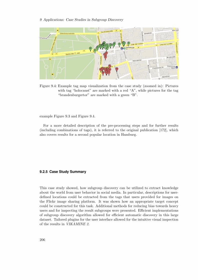
9 Applications: Case Studies in Subgroup Discovery
Figure 9.4: Example tag map visualization from the case study (zoomed in): Pictureswith tag “holocaust” are marked with a red “A”, while pictures for the tag“brandenburgertor” are marked with a green “B”.
example Figure 9.3 and Figure 9.4.
For a more detailed description of the pre-processing steps and for further results(including combinations of tags), it is referred to the original publication [172], whichalso covers results for a second popular location in Hamburg.
9.2.5 Case Study Summary
This case study showed, how subgroup discovery can be utilized to extract knowledgeabout the world from user behavior in social media. In particular, descriptions for user-defined locations could be extracted from the tags that users provided for images onthe Flickr image sharing platform. It was shown how an appropriate target conceptcould be constructed for this task. Additional methods for reducing bias towards heavyusers and for inspecting the result subgroups were presented. Efficient implementationsof subgroup discovery algorithm allowed for efficient automatic discovery in this largedataset. Tailored plugins for the user interface allowed for the intuitive visual inspectionof the results in VIKAMINE 2.
206

9.3 Pattern Mining for Improved Conditional Random Fields
Table 9.3: Brandenburger Tor: top patterns (description size 1) for the ’fuzzified’ targetconcept distance function ranging from 1 km to 5 km.
Tag Subgroup size Mean target value
berlin 113977 0.46reichstag 2604 0.05potsdamerplatz 2017 0.05mitte 3507 0.42berlinmitte 3053 0.30heinrichbollstiftung 1211 0.01hauptstadt 2350 0.34brandenburgertor 1136 0.10alexanderplatz 1699 0.28city 18246 0.76tiergarten 2497 0.42platz 2171 0.4touristen 2815 0.47nachbarn 3691 0.55sonycenter 803 0.02
9.3 Pattern Mining For Improved Conditional Random Fields4
This work so far focused strongly on subgroup discovery as a knowledge discovery tech-nique, that is, the mining of patterns which are aimed directly at domain experts. How-ever, supervised pattern mining can also be exploited in black box machine learningtechniques as subtasks within more sophisticated algorithms. Since the respective pat-tern mining subtasks are algorithmically very similar to subgroup discovery, the efficienttechniques and implementations presented in this work can also be employed in this typeof application.
In that direction, we used supervised pattern mining in a novel approach for informa-tion extraction in domains with context-specific consistencies. The general task was toextract structured information from a text segment, e.g., to extract the author and titlefields from reference sections of scientific papers. State-of-the-art algorithms for thistask are based on conditional random fields [163, 230]. These are undirected, graphical
4This section refers to the previously published works [145] and [146]: (1) Peter Kluegl, Martin Toepfer,Florian Lemmerich, Andreas Hotho, and Frank Puppe: Exploiting Structural Consistencies withStacked Conditional Random Fields, Mathematical Methodologies in Pattern Recognition and Ma-chine Learning, 30:111-125, 2013. (2) Peter Kluegl, Martin Toepfer, Florian Lemmerich, AndreasHotho, and Frank Puppe: Collective information extraction with context-specific consistencies. Eu-ropean Conference on Machine Learning and Knowledge Discovery in Databases (ECML/PKDD),2012. This section only outlines these approach from a subgroup discovery perspective.
207

9 Applications: Case Studies in Subgroup Discovery
probabilistic models, which are commonly applied in machine learning for predictinglabel sequences. The specific approach proposed by our working group exploits thatinstances are not all independent and identically distributed, but are generated in cer-tain contexts that imply similar characteristics. For example, references originate frompapers, which follow different bibliographic styles in different papers. However, they areusually coherently formatted in a single paper. This local consistency is exploited in twonovel methods that both employ supervised pattern mining as subtasks:
In the first algorithm, two conditional random fields are combined in a stacked ap-proach: Initially, a first conditional random field is trained as usual. Then, supervisedpattern mining is applied on all output labels of a certain context to learn descriptionsfor its specific properties in a certain context. For that purpose, tabular training datasetsare constructed, in which each token of the input sequence represents one instance. Asubset of the input features of the conditional random fields is used for the describingattributes. For each possible transition between two labels, one target attribute is cre-ated. Then, for each target attribute one pattern mining task is performed to identifycharacteristic properties for this label transition. The pattern mining results are thenused as additional features to train a second conditional random field that produces thefinal results. In the second approach, the features are similarly discovered, but are addedas additional factors to extend the linear-chain conditional random fields. As a result,both approaches achieved an error reduction of about 30%. For more details on theseapproaches, it is referred to the original papers [147, 146], see also [145].
From a pattern mining point of view this was an interesting task, since efficient compu-tation of the patterns is key: Although the datasets were only medium-sized – a typicaldataset contained about 3000 instances and about 200 binary describing attributes –algorithmic efficiency was required, since many runs of the pattern mining task had tobe performed in the inference step of the conditional random fields. For that purpose thebitset-based algorithm BSD was applied, cf. [177]. Additionally a new interestingnessmeasure qF1exp was requested for the pattern mining tasks:
qF1exp(P ) =2 · pPiP + p∅
·
(1−
(|iP − Ey|
max(iP , Ey)
)2)
The left part of this measure is the traditional F1-measure that describes how well thepattern reproduces the predicted transition. The right factor is a penalty term for thedivergence of the amount of instances classified as boundaries in comparison to a givenexpectation Ey, which is derived from background knowledge. For example, in thedomain of reference segmentation, it is expected that each reference contains exactlyone title segment.
Using the flexible VIKAMINE 2 -kernel architecture, supervised pattern miningcould be easily integrated in the overall algorithm. The efficient implementations ofVIKAMINE 2 allowed to perform the numerous pattern mining tasks efficiently withinthe overall machine learning algorithm.
208

9.4 CaseTrain
9.4 CaseTrain
CaseTrain is an online case-based training system for higher education [120], which iswidely used at the University of Wurzburg. On average, more than 800 training caseswere solved by the students per day in the last years. To evaluate the benefits of thesystem for students, exceptional model mining was applied. Despite the high usage ofthe system, large scale statistical analysis of the usage was difficult since statistics fromthe training system cannot easily be linked to external student data, e.g., for privacyreasons. Therefore, the exceptional model mining focused on a single course with abouttwo hundred users.
For each student, a variety of data was available, most importantly the time thestudents spent with the system and the score in the final exam of the course. Overall,there was a significant correlation between these two attributes with a Pearson coefficientof 0.336. That is, the more time the students spent with the system, the better the examscore for the course was. Even though this might be influenced by confounding factors,it indicates the usefulness of the system. The exceptional model mining now aimed atidentifying influence factors, which alter this correlation between the time spent withthe system and the final score. Therefore, the correlation between these attributes wasused as the target model for the mining task. As interestingness measure, the functionqcor(P ) = iP
a ·(ρP−ρ∅) was applied, where iP is the number of instances in the subgroupand ρP , ρ∅ are the correlation coefficients between the target attributes in the subgroupand the total population respectively.
Two analyses were performed with different describing attributes. The first analysiswas concerned with the question if certain usage patterns are indicators for a stronger orweaker correlation between the overall time spent and the final grade. In that direction,the describing attributes contained information, at which time (relative to the exam) thesystem was used, how many training cases were finished successfully or canceled, andwhat the average achieved score in the training cases was. Here, one result was that thesubgroup of students, who use the system throughout the semester and not only directlybefore the exam, had a higher correlation between training time and score in the finalexam (54 students with a correlation coefficient of 0.480).
In the second analysis, it was investigated if there are certain training cases in thesystem that are especially favorable or unfavorable. For that purpose, additional de-scribing attributes indicated for each training case, how often a student worked withit. One interesting finding was concerned with a certain training case that was markedas a task from a previous exam. The 37 students, which executed this case at leastthree times, had a weak grade with respect to the time they worked with the system:The correlation coefficient between the two target attribute for these students decreasedsubstantially to −0.127, see also Figure 9.5. However, also ignoring tasks from previousexams altogether seemed not to be a good strategy for students: For the 47 students,who did not work at least once with the respective task, the correlation coefficient alsodecreased to 0.017. Thus, it could be concluded that it is most beneficial for studentsto include this task into their exam preparation, but not to focus too much on it. Other
209

9 Applications: Case Studies in Subgroup Discovery
subgroups with larger conjunctive descriptions had larger deviations in the correlationcoefficient, but were also more difficult to interpret.
Overall, exceptional model mining was able to extract interesting, interpretable find-ings. Even though the dataset was comparatively small and subgroup mining was limitedto short subgroup descriptions, identifying these patterns would have been tedious with-out the proper tool support of VIKAMINE 2. The findings could also be visualizedcomfortably using the EDAT-Plugin, Section 8.8.
(a) Overall Population (b) Subgroup
Figure 9.5: Comparison of correlation coefficients between the time spent with the Case-Train system and the score in the final exam of the respective course. Onthe left-hand side the scatterplot with the linear regression line is drawn forthe overall population, on the right-hand it is shown for the subgroup ofstudents, who worked at least three times with a certain training case fromprevious exams.
9.5 Industrial Application
In another project, subgroup discovery was applied on a dataset from the manufacturingdomain. Since the investigated production process is complex, the resulting products aresometimes of insufficient quality or in need of an additional repair step. To identify influ-ence factors that increase or decrease the rate of these faulty parts, subgroup discoverywas applied. Describing information included the time of production (time of the dayand day of the week), environmental variables (e.g., temperature), the group of workersand used materials. Since the mining was performed interactively together with domainexperts, tool support and efficient algorithms were required. Using VIKAMINE 2 andthe SD-Map* algorithm, see Section 4.4.1, for this task enabled the close involvement ofthe domain experts in the discovery process. As one interesting result, the storage tanks
210

9.6 I-Pat Challenge
for certain chemicals played an important role in the production process. Unfortunately,this work cannot provide more details on this project due to privacy issues.
9.6 I-Pat Challenge
The I-Pat challenge was a local pattern mining competition organized for the workshop“Mining and exploiting interpretable local patterns” at the ECML/PKDD 2012. Forthe challenge, a dataset on gene expression analysis was provided. The goal of thisresearch area is to describe sets of genes, which are associated with a certain disease.The dataset consisted of 6172 genes (instances), which were described by more than9000 binary features from a gene ontology. The binary target label indicated if the genewas statistically associated with a certain protein for tumor suppression, cf. also [236].A submission to the challenge consisted of a set of three subgroups that should containinteresting dependencies to this target concept. The subgroups were assessed and scoredby domain experts with to respect novelty, usability and generality.
To evaluate the usefulness of some improvements presented in this work, the authorparticipated in the challenge. As a strategic decision, it was decided to restrict subgroupdescriptions to selection expressions, which indicate the presence of a gene ontology term(feature is set to true), and ignore the absence of features. For the selection of subgroupsit was focused on generalization-aware measures based on the minimum improvementand expectation-driven subgroup discovery with the leaky-noisy-or model, cf. Chapter 7.The efficient algorithms implemented in VIKAMINE 2 allowed to quickly obtain andinspect the results of different parameterizations. From the result subgroups, the finaldecision was made manually, picking subgroups that achieved good scores according toboth, the minimum improvement and the leaky-noisy-or model. It was decided to onlysubmit subgroups descriptions that combine at most two gene terms, since more complexpatterns were assumed to be more complicated to comprehend.
This submission received the best overall average score from the domain experts, beat-ing 6 other submissions of subgroup patterns to win the I-Pat 2012 challenge. Two of thethree submitted subgroup received the maximum score. An interesting general feedbackof domain experts was that many submitted subgroups were too general, contradictinga widely applied intuition for the selection of subgroups.
9.7 Discussion
Several case studies were predominantly performed for pragmatic problem solving inpractical applications. However, also from a research point of view they offer benefits inthree different directions:
First, the documented experiences provide guidance for future practitioners. In thisdirection, detailed descriptions of the respective mining scenarios and applied settingsfor automatic subgroup discovery steps, i.e., the exact interestingness measures, havebeen presented. As one overall result, generalization-aware or expectation-driven inter-estingness measures were considered in most cases as superior to traditional measures.
211

9 Applications: Case Studies in Subgroup Discovery
Second, the case studies were useful to evaluate the implemented techniques. Here,the flexible VIKAMINE 2 software environment showed to be an effective tool for suc-cessful subgroup discovery: Required and helpful additions, such as novel interestingnessmeasures or visualizations could be integrated quickly on demand. Although the sizesof the datasets were limited in most cases, the efficient implementations (including thenovel algorithms presented in Chapters 4, 5, and 6) were often highly useful in reducingthe waiting time of users since automatic discovery steps were often executed multipletimes with slightly modified settings in an iterative approach. However, a large datasetthat ultimately required efficient algorithms was only employed by a single case study,that is, by the mining of patterns in social media. (For the scalability of exceptionalmodel mining in this dataset, see also Section 5.5.2.) Therefore, the performed case stud-ies were not necessarily suited for an efficiency evaluation of the proposed algorithmicimprovements.
Third, case studies can be used to get pointers for future research directions. In thiscontext, it is notable that in all settings most of the discovered interesting subgroups hadrather short descriptions, that is, they were described by a single selector or a conjunctionof two selectors. This may partially be caused by the fact that in the investigatedscenarios subgroup discovery was employed in a reporting-like scenario, in which thedomain experts feedback could only be integrated in few, time-consuming process cycles.Nevertheless, this can be seen as a hint to move the research focus from more and moresophisticated algorithms that discover patterns with long descriptions efficiently towardsefficient algorithms for the discovery of more interesting and less redundant patternsthat potentially involve more complex interestingness measures. In this direction, theextension of expectation-driven interestingness measures to numeric target concepts andexceptional model mining seems beneficial for future applications. Another open issuein that regard is the selection of appropriate, non-redundant descriptions for numericdescribing attributes.
9.8 Summary
This chapter reported on several real-world applications that successfully employed sub-group discovery in diverse domains: Two larger case studies were concerned with theinvestigation of factors that influence the success and satisfaction of university studentsand with the description of geographic locations by using tagging data from the socialweb. Further applications included the application of supervised pattern mining methodsto improve conditional random fields for information extraction, the evaluation of theeducational training system CaseTrain, a minor industrial application, and a submissionto the IPAT pattern mining challenge. Finally, the benefits and limitations of the casestudies were discussed.
212

10 Conclusions
This chapter first summarizes the main contributions of this work. Then, an outlookconcludes the work with some pointers to promising future research directions.
10.1 Summary
Knowledge discovery is concerned with the extraction of novel, statistically valid, inter-pretable, and ultimately useful patterns from large datasets [79]. A key technique forthat purpose is subgroup discovery. Subgroup discovery finds describable subsets in thedata that show an interesting statistical distribution with respect to a certain predefinedtarget concept. Descriptions are usually defined as conjunctions of simple selection ex-pressions over the dataset attributes. Although this problem setting is well-researchedin its basic form, there are still various issues that limit its use in practical applications.To approach these issues, contributions in several directions have been presented in thiswork:
Since subgroup discovery suffers from the curse of dimensionality, the efficiency ofalgorithms is important. Fast algorithms do not only make subgroup discovery tractablefor very large datasets, they also improve the user experience in interactive settings sinceusers can try out many variations of mining tasks with little waiting time. Algorithmicadvances for efficient mining can be categorized in three dimensions: First, the enumer-ation strategy defines, in which order candidate subgroups are explored. Second, thedata structure determines how the data is stored to allow for the efficient evaluation ofcandidates. Third, the pruning strategy allows skipping parts of the search space with-out affecting the optimality of results, e.g., by using optimistic estimate bounds. Theseare upper bounds for the interestingness of all specializations of a subgroup, which areknown to be highly useful for safe pruning of the search space.
Chapter 3 provided a detailed description of these algorithmic components. The cate-gorization of algorithms in these dimensions allowed for a concise description of existingalgorithms. The provided summary of algorithms from literature was not limited tothose using the terminology of subgroup discovery, but also covered approaches fromclosely related fields.
Most efficient algorithms for subgroup discovery concentrate on the basic setting witha binary target concept and an interestingness measure, which is only based on thestatistics of the current subgroup. In this work, efficiency improvements for variousvariants of this standard setting were developed:
In Chapter 4, subgroup discovery with a numeric target concept was investigated. Inthat direction, novel optimistic estimate bounds have been introduced for a large variety
213

10 Conclusions
of interestingness measures. Some of the bounds are expressed in closed forms basedon few key statistics and can be employed in combination with FP-tree-based datastructures. The computation of additional bounds requires a full pass over all subgroupinstances for each evaluation, but results in tighter bounds. Regarding data structures, itwas shown how two different advanced data structures could be adapted for this setting,that is, bitset-based data representations and FP-trees. The proposed improvementswere incorporated in two novel algorithms, that is, the SD-Map* algorithm and theNumBSD algorithm. Both outperform previous approaches by more than an order ofmagnitude.
Exceptional model mining is an extension of classical subgroup discovery that featuresa model over multiple attributes instead of a single attribute as target concept. Chap-ter 5 proposed a novel approach for fast exhaustive exceptional model mining: It adaptsthe FP-tree data structure for exceptional model mining in a generic way. This is ac-complished by introducing the concept of valuation bases as an intermediate condenseddata representation. Many, but not all model classes are suited for that approach. Therespective model classes were characterized by a theorem that draws an analogy to datastream mining. Concrete implementations of the generic approach for several modelclasses could be derived and lead to runtime improvements of more than an order ofmagnitude in comparison to a naive exhaustive depth-first-search.
The interestingness measures for subgroup selection are traditionally based exclu-sively on the statistics of the evaluated subgroup. Recently, subgroup discovery withgeneralization-aware interestingness measures has received increased attention in theresearch community. These measures compare the share of the target concept in thesubgroup not only with the target share in the overall dataset, but also with the targetshares of all generalizations of the current subgroup. In doing so, redundant findings areavoided and more interesting subgroups are discovered. In order to improve algorith-mic efficiency in this setting, Chapter 6 introduced a new method of deriving optimisticestimates for subgroup discovery with these interestingness measures. In contrast toprevious approaches to derive optimistic estimates, the novel bounds are not only basedon the anti-monotonicity of instances covered by a subgroup, but incorporate also thedifference in coverage between the subgroup and its generalizations. The incorpora-tion of the new optimistic estimates in state-of-the-art algorithms improved the runtimerequirements by more than an order of magnitude in many cases.
The previously mentioned contributions focus on the efficiency of algorithms. Thatis, the proposed automatic discovery algorithms produce the same results as existingalgorithms, but require substantially less time. Other contributions improve the effec-tiveness of subgroup discovery. That means that the produced results are closer to whatis wanted in actual applications.
In that direction, Chapter 7 presented the novel concept of expectation-driven subgroupdiscovery. It introduced a novel family of interestingness measures in order to achievemore interesting subgroup discovery results. For that purpose, the expectations onthe target share of a subgroup with a binary target concept are estimated using thestatistics for the separate influence factors, which are combined to describe the subgroup.The difference between the expected and the actual target shares then determines the
214

10.2 Outlook
interestingness of a subgroup. Since expectations are inherently subjective, there is nota single correct function to compute them. However, plausible values, which are in linewith human reasoning, can be achieved by transferring techniques from the researchon bayesian networks to the subgroup discovery setting. The generation of bayesiannetwork fragments as local models allowed to apply well known methods of this researcharea, e.g., the leaky-nosiy-or model or the logit model. The novel approach resultedin qualitatively different subgroups than traditional approaches, unveiling previouslyundiscovered relations. The usefulness of this approach could be demonstrated in severalexperiments, including two real-world case studies.
Beside these more theoretical core contributions, also practical issues were approached:Subgroup discovery is not an isolated automatic process, but an iterative and interac-tive task, which requires a flexible, interactive mining environment. For that purpose,the VIKAMINE 2 tool was developed in the context of this work, which significantlyimproves and extends its predecessor, see Chapter 8. It provides a broad collection ofstate-of-the-art algorithms and interestingness measures for mining with binary as wellas numeric target concepts, including novel methods proposed in this work. A new,appealing graphical user interface based on the Eclipse RCP framework enables easyextensibility. Additionally, it features novel methods for the interactive mining in largedatasets, e.g., the dynamic subgroup tree, and the effective presentation of results, e.g.,the pie circle visualization and the subgroup treetable. The EDAT plugin provides ad-ditional options for inspecting the statistical properties in the overall dataset as well asin specific subgroups by utilizing a bridge to the statistical language R.
The benefits of the novel techniques contributed to efficient and effective subgroupdiscovery in several real world applications, see Chapter 9. In the educational domain,subgroup discovery was successfully applied to discover parameters that affect the successrate of university students and to find influence factors on the students’ satisfactionrating in a large survey dataset. In the application area of social web mining, subgroupdiscovery was used to describe certain geographic locations by interpreting tags forgeo-referenced images crawled from the Flickr platform. Further application examplesincluded pattern mining for improved information extraction with conditional randomfields, an industrial application regarding the fault rate of products, and a challengedataset regarding gene data analysis.
10.2 Outlook
This work presented several novel techniques that improve the efficiency and effectivenessof subgroup discovery. These contributions also encourage the exploration of ideas infuture research:
Regarding efficiency, the exploitation of optimistic estimate bounds for fast exceptionalmodel mining could lead to substantial performance gains. Especially the explorationof difference-based optimistic estimates could be interesting in this area. Since interest-ingness measures and model classes in this area are heterogeneous, the identification ofcategorizing properties would allow for more generic, widely applicable bounds. In sub-
215

10 Conclusions
group discovery with binary targets, tight optimistic estimates are still to be developedfor expectation-driven interestingness measures. Here, also intelligent caching strate-gies could be beneficial to reduce the memory requirements of algorithms. In order toavoid the discovery of redundant subgroups, the topic of subgroup set mining will quitepossibly receive increased attention in future research. In that area, the explorationof efficient mining algorithms has started only recently. Additionally, the distributionof subgroup discovery tasks to a network of computational nodes provides for interest-ing challenges, in particular the propagation of optimistic estimate bounds with limitedcommunication costs.
Regarding the effectiveness of subgroup discovery, improving the interestingness mea-sures for automatic discovery is still a challenge. In that direction, the extension ofexpectation-driven subgroup discovery to settings with numeric or exceptional modelmining targets seems promising. In order to explore, what results human users reallyperceive as interesting or useful, larger quantitative studies of interestingness measureare desirable. Another open issue is concerned with the redundancy of discovered sub-groups. In particular, avoiding redundant findings for subgroup descriptions that in-volve numeric attributes still is an open issue. While several recent approaches aimat reducing the redundancy of results, e.g., weighted covering, subgroup set mining,or generalization-aware interestingness measures, a thorough comparison of these ap-proaches is still missing in literature. However, dealing with redundant discoveries isquite possibly not only an issue of algorithmic tuning, but also of human-computerinteraction and interface design. For that purpose, further adjustments of subgroupdiscovery tools will be required.
Subgroup discovery has been established as an important technique for knowledgediscovery in order to extract useful findings from large amounts of raw data. However,practical applications of subgroup discovery still involve critical and unexplored chal-lenges. This encourages further scientific research in this field. There is still much todiscover.
216

Bibliography
[1] Poll: Data Mining Methodology, website:http://www.kdnuggets.com/polls/2007/data mining methodology.htm, 2007.
[2] Tarek Abudawood and Peter Flach. First-Order Multi-class Subgroup Discovery.In Proceedings of the 5th Starting AI Researchers’ Symposium at STAIRS, 2010.
[3] Tarek Abudawood and Peter A. Flach. Evaluation Measures for Multi-class Sub-group Discovery. In Proceedings of the European Conference on Machine Learningand Knowledge Discovery in Databases (ECML/PKDD), 2009.
[4] Rakesh Agrawal, Tomasz Imielienski, and Arun Swami. Mining Association Rulesbetween Sets of Items in Large Databases. In Proceedings of the 1993 ACMSIGMOD International Conference on Management of Data, 1993.
[5] Rakesh Agrawal and Giuseppe Psaila. Active Data Mining. In Proceedings of the1st International Conference on Knowledge Discovery and Data Mining (KDD),1995.
[6] Rakesh Agrawal and John C. Shafer. Parallel Mining of Association Rules. IEEETransactions on Knowledge and Data Engineering, 8(6):962–969, 1996.
[7] Rakesh Agrawal and Ramakrishnan Srikant. Fast Algorithms for Mining Associ-ation Rules. In Proceedings of the 20th International Conference on Very LargeData Bases (VLDB), 1994.
[8] Shane Ahern, Mor Naaman, Rahul Nair, and Jeannie Yang. World Explorer: Vi-sualizing Aggregate Data from Unstructured Text in Geo-Referenced Collections.In Proceedings of the 7th ACM/IEEE-CS Joint Conference on Digital Libraries(JCDL), 2007.
[9] Jesus Alcala-Fdez, Alberto Fernandez, Julian Luengo, Joaquin Derrac, SalvadorGarcia, Luciano Sanchez, and Francisco Herrera. KEEL Data-Mining SoftwareTool: Data Set Repository, Integration of Algorithms and Experimental AnalysisFramework. Journal of Multiple-Valued Logic and Soft Computing, 17(2–3):255–287, 2011.
[10] Grigoris Antoniou and Frank Van Harmelen. A Semantic Web Primer. MIT Press,2004.
217

Bibliography
[11] John M. Aronis, Foster J. Provost, and Bruce G. Buchanan. Exploiting Back-ground Knowledge in Automated Discovery. In Proceedings of the 2nd Interna-tional Conference on Knowledge Discovery and Data Mining (KDD), 1996.
[12] Bavani Arunasalam and Sanjay Chawla. CCCS: A Top-down Associative Classifierfor Imbalanced Class Distribution. In Proceedings of the 12th ACM SIGKDDConference on Knowledge Discovery and Data Mining (KDD), 2006.
[13] A. Asuncion and D. J. Newman. UCI Machine Learning Repository:http://www.ics.uci.edu/∼mlearn/MLRepository.html, 2007.
[14] Martin Atzmueller. Knowledge-Intensive Subgroup Mining - Techniques for Auto-matic and Interactive Discovery. PhD thesis, University of Wurzburg, 2006.
[15] Martin Atzmueller and Florian Lemmerich. Fast Subgroup Discovery for Contin-uous Target Concepts. In Proceedings of the 18th International Symposium onFoundations of Intelligent Systems (ISMIS), 2009.
[16] Martin Atzmueller and Florian Lemmerich. VIKAMINE - Open-Source Sub-group Discovery, Pattern Mining, and Analytics. In Proceedings of the Euro-pean Conference on Machine Learning and Knowledge Discovery in Databases(ECML/PKDD), 2012.
[17] Martin Atzmueller and Florian Lemmerich. Exploratory Pattern Mining on So-cial Media using Geo-References and Social Tagging Information. InternationalJournal of Web Science, 2(1–2):80–112, 2013.
[18] Martin Atzmueller, Florian Lemmerich, Beate Krause, and Andreas Hotho. To-wards Understanding Spammers - Discovering Local Patterns for Concept Descrip-tion. In From Local Patterns to Global Models, Workhop at the ECML/PKDD,2009.
[19] Martin Atzmueller and Folke Mitzlaff. Efficient Descriptive Community Mining. InProceedings of the 24th Florida Artificial Intelligence Research Society Conference(FLAIRS), 2011.
[20] Martin Atzmueller and Frank Puppe. Semi-Automatic Visual Subgroup Miningusing VIKAMINE. Journal of Universal Computer Science, 11(11):1752–1765,2005.
[21] Martin Atzmueller and Frank Puppe. A Methodological View on Knowledge-Intensive Subgroup Discovery. In Proceedings of the 9th European Knowledge Ac-quisition Workshop (EKAW), 2006.
[22] Martin Atzmueller and Frank Puppe. SD-Map - A Fast Algorithm for ExhaustiveSubgroup Discovery. In Proceedings of the 10th European Conference on Principlesand Practice of Knowledge Discovery in Databases (PKDD), 2006.
218

Bibliography
[23] Martin Atzmueller and Frank Puppe. Semi-Automatic Refinement and Assessmentof Subgroup Patterns. In Proceedings of the 21th International Florida ArtificialIntelligence Research Society Conference (FLAIRS), 2008.
[24] Martin Atzmueller and Frank Puppe. A Knowledge-Intensive Approach for Semi-Automatic Causal Subgroup Discovery. In Bettina Berendt et al., editors, Knowl-edge Discovery Enhanced with Semantic and Social Information, volume 220, pages19–36. 2009.
[25] Martin Atzmueller, Frank Puppe, and Hans-Peter Buscher. Exploiting BackgroundKnowledge for Knowledge-Intensive Subgroup Discovery. In Proceedings of the 19thInternational Joint Conference on Artificial Intelligence (IJCAI), 2005.
[26] Martin Atzmueller, Frank Puppe, and Hans-Peter Buscher. A Semi-AutomaticApproach for Confounding-Aware Subgroup Discovery. International Journal onArtificial Intelligence Tools, 18(1):81–98, 2009.
[27] Yonatan Aumann and Yehuda Lindell. A Statistical Theory for Quantitative Asso-ciation Rules. In Proceedings of the 5th ACM SIGKDD International Conferenceon Knowledge Discovery and Data Mining (KDD), 1999.
[28] Yonatan Aumann and Yehuda Lindell. A Statistical Theory for Quantitative As-sociation Rules. Journal of Intelligent Information Systems, 20(3):255–283, 2003.
[29] Iyad Batal and Milos Hauskrecht. A Concise Representation of Association Rulesusing Minimal Predictive Rules. In Proceedings of the 2010 European Conferenceon Machine Learning and Knowledge Discovery in Databases (ECML/PKDD),2010.
[30] Iyad Batal and Milos Hauskrecht. Constructing Classication Features Using Mini-mal Predictive Patterns. In Proceedings of the 19th ACM International Symposiumon High Performance Distributed Computing, 2010.
[31] Joachim Baumeister, Martin Atzmueller, and Frank Puppe. Inductive Learningfor Case-Based Diagnosis with Multiple Faults. In Proceedings of the 9th EuropeanConference on Advances in Case-Based Reasoning, 2002.
[32] Stephen D. Bay and Michael J. Pazzani. Detecting Change in Categorical Data:Mining Contrast Sets. In Proceedings of the 5th ACM SIGKDD InternationalConference on Knowledge Discovery and Data Mining (KDD), 1999.
[33] Stephen D. Bay and Michael J. Pazzani. Detecting Group Differences: MiningContrast Sets. Data Mining and Knowledge Discovery, 5(3):213–246, 2001.
[34] Roberto J. Bayardo. Efficiently Mining Long Patterns from Databases. In Pro-ceedings of the 1998 ACM SIGMOD International Conference on Management ofData, 1998.
219

Bibliography
[35] Roberto J. Bayardo, Rakesh Agrawal, and Dimitrios Gunopulos. Constraint-BasedRule Mining in Large, Dense Databases. Data Mining and Knowledge Discovery,4(2–3):217–240, 1999.
[36] Martin Becker. Constraint Based Descriptive Pattern Mining. Diploma Thesis,Supervised by the author of this work, University of Wurzburg, 2011.
[37] Yoav Benjamini and Yosef Hochberg. Controlling the False Discovery Rate: APractical and Powerful Approach to Multiple Testing. Journal of the Royal Sta-tistical Society. Series B (Methodological), 57(1):289–300, 1995.
[38] Janine Bennett, Ray Grout, Philippe Pebay, Diana Roe, and David Thomp-son. Numerically Stable, Single-Pass, Parallel Statistics Algorithms. In Proceed-ings of the IEEE International Conference on Cluster Computing and Workshops(CLUSTER), 2009.
[39] Francisco Berlanga, Marıa Jose del Jesus, Pedro Gonzalez, Francisco Herrera, andMikel Mesonero. Multiobjective Evolutionary Induction of Subgroup DiscoveryFuzzy Rules: A Case Study in Marketing. In Proceedings of the 6th IndustrialConference on Data Mining (ICDM), 2006.
[40] Tijl De Bie, Kleanthis-Nikolaos Kontonasios, and Eirini Spyropoulou. A Frame-work for Mining Interesting Pattern Sets. In Workshop on Useful Patterns, Work-shop at the ACM SIGKDD, 2010.
[41] Mario Boley, Thomas Gartner, and Henrik Grosskreutz. Formal Concept Samplingfor Counting and Threshold-Free Local Pattern Mining. In Proceedings of the 10thSIAM International Conference on Data Mining (SDM), 2010.
[42] Mario Boley and Henrik Grosskreutz. Approximating the Number of FrequentSets in Dense Data. Knowledge and Information Systems, 21(1):65–89, 2009.
[43] Mario Boley, Claudio Lucchese, Daniel Paurat, and Thomas Gartner. Direct LocalPattern Sampling by Efficient Two-Step Random Procedures. In Proceedings ofthe 17th ACM SIGKDD International Conference on Knowledge Discovery andData Mining (KDD), 2011.
[44] George E. P. Box. Non-Normality and Tests on Variances. Biometrika, 40:318–335,1953.
[45] Leo Breiman, Jerome H. Friedman, Charles J. Stone, and Richard A. Olshen.Classification and Regression Trees. Chapman & Hall, 1984.
[46] Sergey Brin, Rajeev Rastogi, and Kyuseok Shim. Mining Optimized Gain Rulesfor Numeric Attributes. In Proceedings of the 5th ACM SIGKDD InternationalConference on Knowledge Discovery and Data Mining, 2003.
[47] Bjorn Bringmann, Siegfried Nijssen, and Albrecht Zimmermann. Pattern-BasedClassification: A Unifying Perspective, arXiv preprint arXiv:1111.6191, 2011.
220
Bibliography
[48] Bjorn Bringmann, Albrecht Zimmermann, Luc De Raedt, and Siegfried Nijssen.Don’t Be Afraid of Simpler Patterns. In Proceedings of the 10th European con-ference on Principle and Practice of Knowledge Discovery in Databases (PKDD),2006.
[49] Herve Broennimann, Bin Chen, Manoranjam Dash, Peter Haas, Yi Qiao, andPeter Scheuermann. Efficient Data-Reduction Methods for On-Line AssociationRule Discovery. In Data Mining: Next-Generation Challenges and Future Direc-tions, Selected Papers from the NSF Workshop on Next-Generation Data Mining(NGDM), 2004.
[50] Facundo Bromberg, Brian Patterson, and Sandeep Yaramakala. Mining BayesianNetworks from Streamed Data. Technical report, Iowa State University, Ames,2003.
[51] Gregory Buehrer, Srinivasan Parthasarathy, Shirish Tatikonda, Tahsin Kurc, andJoel Saltz. Toward Terabyte Pattern Mining: An Architecture-conscious Solution.In Proceedings of the 12th ACM SIGPLAN Symposium on Principles and Practiceof Parallel Programming, 2007.
[52] Toon Calders and Bart Goethals. Mining All Non-Derivable Frequent Itemsets.In Proceedings of the 6th European Conference on Principles of Data Mining andKnowledge Discovery (PKDD), 2002.
[53] Toon Calders and Bart Goethals. Depth-First Non-Derivable ItemsetMining. InProceedings of the 5th SIAM International Conference on Data Mining (SDM),2005.
[54] Toon Calders and Bart Goethals. Non-Derivable Itemset Mining. Data Miningand Knowledge Discovery, 14(1):171–206, 2007.
[55] Jose-Ramon Cano, Salvador Garcıa, and Francisco Herrera. Subgroup Discovery inLarge Size Data Sets Preprocessed using Stratified Instance Selection for Increasingthe Presence of Minority Classes. Pattern Recognition Letters, 29:2156–2164, 2008.
[56] Jose-Ramon Cano, Francisco Herrera, Manuel Lozano, and Salvador Garcıa. Mak-ing CN2-SD Subgroup Discovery Algorithm Scalable to Large Size Data Sets usingInstance Selection. Expert Systems with Applications, 35(4):1949–1965, 2008.
[57] Loic Cerf, Dominique Gay, Nazha Selmaoui, and Jean-Francois Boulicaut. AParameter-Free Associative Classification Method. In Proceedings of the 10th In-ternational Conference on Data Warehousing and Knowledge Discovery (DaWaK),2008.
[58] Bin Chen, Peter Haas, and Peter Scheuermann. A New Two-Phase SamplingBased Algorithm for Discovering Association Rules. In Proceedings of the 8thACM SIGKDD International Conference on Knowledge Discovery and Data Min-ing (KDD), 2002.
221

Bibliography
[59] Hong Cheng, Xifeng Yan, Jiawei Han, and Chih-Wei Hsu. Discriminative FrequentPattern Analysis for Effective Classification. In Proceedings of the 23rd Interna-tional Conference on Data Engineering (ICDE), 2007.
[60] Hong Cheng, Xifeng Yan, Jiawei Han, and Philip S. Yu. Direct DiscriminativePattern Mining for Effective Classification. In Proceedings of the 24th InternationalConference on Data Engineering (ICDE), 2008.
[61] David W. Cheung, Jiawei Han, Vincent T. Ng, Ada W. Fu, and Yongjian Fu. AFast Distributed Algorithm for Mining Association Rules. In Proceedings of the 4thInternational Conference on Parallel and Distributed Information Systems, 1996.
[62] Peter Clark and Robin Boswell. Rule Induction with CN2: Some Recent Improve-ments. In Proceedings of the European Working Session on Machine Learning(EWSL), 1991.
[63] Peter Clark and Tim Niblett. The CN2 Induction Algorithm. Machine Learning,3(4):261–283, 1989.
[64] William W. Cohen. Fast Effective Rule Induction. In Proceedings of the 11thInternational Conference on Machine Learning (ICML), 1995.
[65] R. J. Dakin. A Tree-search Algorithm for Mixed Integer Programming Problems.The Computer Journal, 8(3):250–255, 1965.
[66] Olena Daly and David Taniar. Exception Rules in Data Mining. In MehdiKhosrow-Pour, editor, Encyclopedia of Information Science and Technology (II),pages 1144–1148. 2005.
[67] Luc De Raedt, Tias Guns, and Siegfried Nijssen. Constraint Programming forItemset Mining. In Proceeding of the 14th ACM SIGKDD International Conferenceon Knowledge Discovery and Data Mining (KDD), 2008.
[68] Marıa Jose del Jesus and Pedro Gonzalez. Evolutionary Fuzzy Rule InductionProcess for Subgroup Discovery: A Case Study in Marketing. IEEE Transactionson Fuzzy Systems, 15(4):578–592, 2007.
[69] Francisco J. Diez and Marek J. Druzdzel. Canonical Probabilistic Models forKnowledge Engineering. Technical report, Universidad Nacional de Educacion aDistancia Madrid, 2006.
[70] Guozhu Dong and Jinyan Li. Efficient Mining of Emerging Patterns: DiscoveringTrends and Differences. In Proceedings of the 5th ACM SIGKDD InternationalConference on Knowledge Discovery and Data Mining (KDD), 1999.
[71] Wouter Duivesteijn, Ad Feelders, and Arno J. Knobbe. Different Slopes for Dif-ferent Folks - Mining for Exceptional Regression Models with Cook’s Distance. InProceedings of the 18th ACM SIGKDD International Conference on KnowledgeDiscovery and Data Mining (KDD), 2012.
222

Bibliography
[72] Wouter Duivesteijn and Arno J. Knobbe. Exploiting False Discoveries – StatisticalValidation of Patterns and Quality Measures in Subgroup Discovery. In Proceedingsof the 11th International Conference on Data Mining (ICDM), 2011.
[73] Wouter Duivesteijn, Arno J. Knobbe, Ad Feelders, and Matthijs van Leeuwen.Subgroup Discovery Meets Bayesian Networks – An Exceptional Model Miningapproach. In Proceedings of the 10th International Conference on Data Mining(ICDM), 2010.
[74] Olive J. Dunn. Multiple Comparisons Among Means. Journal of the AmericanStatistical Association, 56(293):52–64, 1961.
[75] Vladimir Dzyuba and Matthijs van Leeuwen. Interactive Discovery of InterestingSubgroup Sets. Proceedings of the 12th International Symposium on Advances inIntelligent Data Analysis (IDA), 2013.
[76] Eyas El-Qawasmeh. Beating the Popcount. International Journal of InformationTechnology, 9(1):1–18, 2003.
[77] Tom Fawcett. An Introduction to ROC Analysis. Pattern Recognition Letters,27(8):861–874, 2006.
[78] Usama M. Fayyad and Keki B. Irani. Multi-Interval Discretization of Continuous-Valued Attributes for Classification Learning. In Proceedings of the 13th Interna-tional Joint Conference on Artificial Intelligence (IJCAI), 1993.
[79] Usama M. Fayyad, Gregory Piatetsky-Shapiro, and Padhraic Smyth. Advancesin Knowledge Discovery and Data Mining: An Overview. In Usama M. Fayyad,Gregory Piatetsky-Shapiro, Padhraic Smyth, and Ramasamy Uthurusamy, editors,Advances in Knowledge Discovery and Data Mining, pages 1–34. 1996.
[80] Usama M. Fayyad, Gregory Piatetsky-Shapiro, and Padhraic Smyth. From DataMining to Knowledge Discovery in Databases. AI magazine, 17(3):37–54, 1996.
[81] Alex A. Freitas. On Rule Interestingness Measures. Knowledge-Based Systems,12:309–315, 1999.
[82] Jerome H. Friedman and Nicholas I. Fisher. Bump Hunting in High-dimensionalData. Statistics and Computing, 9(2):123–143, 1999.
[83] Marlene Fries. Welchen Wert hat das Abitur fur ein erfolgreiches Studium?Beitrage zur Hochschulforschung, 1:30–51, 2002.
[84] Takeshi Fukuda, Yasuhiko Morimoto, Shinichi Morishita, and Takeshi Tokuyama.Mining Optimized Association Rules for Numeric Attributes. In Proceedings of the15th ACM Symposium on Principles of Database Systems (PODS), 1996.
223

Bibliography
[85] Johannes Furnkranz and Peter A. Flach. ROC ’n’ rule Rule Learning - Towardsa Better Understanding of Covering Algorithms. Machine Learning, 58(1):39–7,2005.
[86] Johannes Furnkranz, Dragan Gamberger, and Nada Lavrac. Foundations of RuleLearning. Springer, 2012.
[87] Johannes Furnkranz, Dragan Gamberger, and Nada Lavrac. Rule Learning in aNutshell. In Johannes Furnkranz, Dragan Gamberger, and Nada Lavrac, editors,Foundations of Rule Learning, pages 19–55. 2012.
[88] Johannes Furnkranz, Dragan Gamberger, and Nada Lavrac. Supervised Descrip-tive Rule Learning. In Johannes Furnkranz, Dragan Gamberger, and Nada Lavrac,editors, Foundations of Rule Learning, pages 247–265. 2012.
[89] Johannes Furnkranz and Georg Widmer. Incremental Reduced Error Pruning. InProceedings of the International Conference on Machine Learning (ICML), 1994.
[90] Brian R. Gaines. Knowledge Acquisition: Past, Present and Future. InternationalJournal of Human-Computer Studies, 71(2):135–156, 2013.
[91] Dragan Gamberger and Nada Lavrac. Expert-Guided Subgroup Discovery:Methodology and Application. Journal of Artificial Intelligence Research, 17:501–527, 2002.
[92] Dragan Gamberger, Nada Lavrac, and Goran Krstacic. Active Subgroup Mining: aCase Study in Coronary Heart Disease Risk Group Detection. Artificial Intelligencein Medicine, 28(1):27–57, 2003.
[93] Dragan Gamberger, Nada Lavrac, and Dietrich Wettschereck. Subgroup Visu-alization: A Method and Application in Population Screening. In Proceedingsof the 7th International Workshop on Intelligent Data Analysis in Medicine andPharmacology (IDAMAP-02), 2002.
[94] Salvador Garcıa, Julian Luengo, Jose A. Saez, Victoria Lopez, and Francisco Her-rera. A Survey of Discretization Techniques: Taxonomy and Empirical Analysisin Supervised Learning. IEEE Transactions on Knowledge and Data Engineering,25(4):734–750, 2013.
[95] Gemma C. Garriga, Petra Kralj Novak, and Nada Lavrac. Closed Sets for LabeledData. In Proceedings of the 10th European Conference on Principles and Practiceof Knowledge Discovery in Databases (PKDD), 2006.
[96] Gemma C. Garriga, Petra Kralj Novak, and Nada Lavrac. Closed Sets for LabeledData. Journal of Machine Learning Research (extended version of the identicallytitled conference paper), 9:559–580, 2008.
[97] Liqiang Geng and Howard J. Hamilton. Interestingness Measures for Data Mining:A Survey. ACM Computing Surveys, 38(3): Article no. 9, 2006.
224

Bibliography
[98] Aristides Gionis, Heikki Mannila, Taneli Mielikainen, and Panayiotis Tsaparas.Assessing Data Mining Results via Swap Randomization. ACM Transactions onKnowledge Discovery from Data, 1(3): Article number 14, 2007.
[99] David E. Goldberg. Genetic Algorithms in Search, Optimization, and MachineLearning. Addison Wesley, 1989.
[100] Henrik Grosskreutz. Cascaded Subgroups Discovery with an Application to Regres-sion. In From Local Patterns to Global Models, Workshop at the ECML/PKDD,2008.
[101] Henrik Grosskreutz. Class Relevant Pattern Mining in Output-Polynomial Time.In Proceedings of the 12th SIAM International Conference on Data Mining (SDM),2012.
[102] Henrik Grosskreutz, Mario Boley, and Maike Krause-Traudes. Subgroup Discoveryfor Election Analysis: A Case Study in Descriptive Data Mining. In Proceedingsof the 13th International Conference on Discovery Science (DS), 2010.
[103] Henrik Grosskreutz, Benedikt Lemmen, and Stefan Ruping. Secure DistributedSubgroup Discovery in Horizontally Partitioned Data. Transactions on Data Pri-vacy, 4(3):147–165, 2011.
[104] Henrik Grosskreutz and Daniel Paurat. Fast and Memory-Efficient Discovery ofthe Top-k Relevant Subgroups in a Reduced Candidate Space. In Proceedings ofthe 2011 European Conference on Machine Learning and Knowledge Discovery inDatabases (ECML/PKDD), 2011.
[105] Henrik Grosskreutz, Daniel Paurat, and Stefan Ruping. An Enhanced RelevanceCriterion For More Concise Supervised Pattern Discovery. In Proceedings of the18th ACM SIGKDD International Conference on Knowledge Discovery and DataMining (KDD), 2012.
[106] Henrik Grosskreutz and Stefan Ruping. On Subgroup Discovery in NumericalDomains. Data Mining and Knowledge Discovery, 19(2):210–226, 2009.
[107] Henrik Grosskreutz, Stefan Ruping, Nuhad Shaabani, and Stefan Wrobel. Opti-mistic Estimate Pruning Strategies for Fast Exhaustive Subgroup Discovery. Tech-nical report, Fraunhofer IAIS, 2008.
[108] Henrik Grosskreutz, Stefan Ruping, and Stefan Wrobel. Tight OptimisticEstimates for Fast Subgroup Discovery. In Proceedings of the 2008 Euro-pean Conference on Machine Learning and Knowledge Discovery in Databases(ECML/PKDD), 2008.
[109] Jiawei Han, Hong Cheng, Dong Xin, and Xifeng Yan. Frequent Pattern Mining:Current Status and Future Directions. Data Mining and Knowledge Discovery,15(1):55–86, 2007.
225

Bibliography
[110] Jiawei Han, Micheline Kamber, and Jian Pei. Data Mining: Concepts and Tech-niques. Morgan Kaufmann, 2006.
[111] Jiawei Han, Jian Pei, and Yiwen Yin. Mining Frequent Patterns without CandidateGeneration. ACM SIGMOD Record, 29(2):1–12, 2000.
[112] Jiawei Han, Jian Pei, Yiwen Yin, and Runying Mao. Mining Frequent Patternswithout Candidate Generation: A Frequent-Pattern Tree Approach. Data Miningand Knowledge Discovery, 8(1):53–87, 2004.
[113] Anna Hart. Knowledge Acquisition for Expert Systems. Technical report, Schoolof Computing, Lancashire Polytechnic, Preston, 1986.
[114] Frederick Hayes-Roth, Donald Waterman, and Douglas Lenat. Building ExpertSystems. Addison Wesley, 1984.
[115] David Heckerman and John S Breese. Causal Independence for Probability As-sessment and Inference using Bayesian Networks. IEEE Transactions on Systems,Man and Cybernetics, Part A: Systems and Humans, 26(6):826–831, 1996.
[116] Max Henrion. Practical Issues in Constructing a Bayes’ Belief Network. In Pro-ceedings of the 3rd Annual Conference on Uncertainty in Artificial Intelligence,1987.
[117] Francisco Herrera, Cristobal Jose Carmona, Pedro Gonzalez, and Marıa Josedel Jesus. An Overview on Subgroup Discovery: Foundations and Applications.Knowledge and Information Systems, 29(3):495–525, 2010.
[118] David C. Hoaglin, Frederick Mosteller, and John Wilder Tukey. UnderstandingRobust and Exploratory Data Analysis. Wiley New York, 1983.
[119] Yosef Hochberg and Ajit C. Tamhane. Multiple Comparison Procedures. WileyNew York, 1987.
[120] Alexander Hoernlein, Marianus Ifland, Peter Kluegl, and Frank Puppe. Konzep-tion und Evaluation eines fallbasierten Trainingssystems im universitatsweiten Ein-satz (CaseTrain). GMS Medizinische Informatik Biometrie Epidemiologie 2009,5(1):Doc07, 2009.
[121] Lawrence B. Holder, Diane J. Cook, and Surnjani Djoko. Substructure Discoveryin the SUBDUE System. In Proceedings of the Workshop on Knowledge Discoveryin Databases, 1994.
[122] Sture Holm. A Simple Sequentially Rejective Multiple Test Procedure. Scandina-vian Journal of Statistics, 6(2):65–70, 1979.
[123] Jian Hu and Xiang Yang-Li. A Fast Parallel Association Rules Mining AlgorithmBased on FP-Forest. In Proceedings of the 5th International Symposium on NeuralNetworks (ISNN), 2008.
226

Bibliography
[124] Farhad Hussain, Huan Liu, Einoshin Suzuki, and Hongjun Lu. Exception RuleMining with a Relative Interestingness Measure. In Proceedings of the 4th Pacific-Asia Conference on Knowledge Discovery and Data Mining (PAKDD), 2000.
[125] Frederik Janssen and Johannes Furnkranz. On the Quest for Optimal Rule Learn-ing Heuristics. 78(3):343–379, 2010.
[126] Szymon Jaroszewicz and Tobias Scheffer. Fast Discovery of Unexpected Patternsin Data, Relative to a Bayesian Network. In Proceeding of the 11th ACM SIGKDDInternational Conference on Knowledge Discovery and Data Mining (KDD), 2005.
[127] Szymon Jaroszewicz, Tobias Scheffer, and Dan A. Simovici. Scalable Pattern Min-ing with Bayesian Networks as Background Knowledge. Data Mining and Knowl-edge Discovery, 18(1):56–100, 2008.
[128] David D. Jensen. Knowledge Evaluation: Statistical Evaluations. In Willi Klosgenand Jan M. Zytkow, editors, Handbook of Data Mining and Knowledge Discovery,pages 475–489. 2002.
[129] Kenneth Jensen. Crisp-DM process. website:http://en.wikipedia.org/wiki/File:CRISP-DM Process, 2012.
[130] Alipio M. Jorge, Paulo J. Azevedo, and Fernando Pereira. Distribution Rules withNumeric Attributes of Interest. In Proceedings of the 10th European Conferenceon Principles and Practice of Knowledge Discovery in Databases (PKDD), 2006.
[131] Viktor Jovanoski and Nada Lavrac. Classification Rule Learning with APRIORI-C. In Proceedings of the 10th Portuguese Conference on Progress in ArtificialIntelligence, Knowledge Extraction, Multi-agent Systems, Logic Programming andConstraint Solving (EPIA), 2001.
[132] Andreas M. Kaplan and Michael Haenlein. Users of the World, Unite! The Chal-lenges and Opportunities of Social Media. Business Horizons, 53(1):59–68, 2010.
[133] Kenneth A. Kaufman and Ryszard S. Michalski. Learning From Inconsistent andNoisy Data: The AQ18 Approach. In Proceedings of the 11th Symposium ISMIS,1999.
[134] Branko Kavsek and Nada Lavrac. Analysis of Example Weighting in SubgroupDiscovery by Comparison of Three Algorithms on a Real-life Data Set. In Advancesin Inductive Rule Learning, Workshop at the ECML/PKDD, 2004.
[135] Branko Kavsek and Nada Lavrac. Apriori-SD: Adapting Association Rule LearningTo Subgroup Discovery. Applied Artificial Intelligence, 20:543–583, 2006.
[136] Randy Kerber. Chimerge: Discretization of Numeric Attributes. In Proceedingsof the 10th National Conference on Artificial Intelligence, 1992.
227

Bibliography
[137] Mika Klemettinen, Heikki Mannila, Pirjo Ronkainen, Hannu Toivonen, andA. Inkeri Verkamo. Finding Interesting Rules from Large Sets of Discovered Asso-ciation Rules. In Proceedings of the 3rd International Conference on Informationand Knowledge Management, 1994.
[138] Willi Klosgen. Exploration of Simulation Experiments by Discovery. TechnicalReport WS-04-03, 1994.
[139] Willi Klosgen. Efficient Discovery of Interesting Statements in Databases. Journalof Intelligent Information Systems, 4(1):53–69, 1995.
[140] Willi Klosgen. Explora: A Multipattern and Multistrategy Discovery Assistant. InUsama M. Fayyad, Gregory Piatetsky-Shapiro, Padhraic Smyth, and RamasamyUthurusamy, editors, Advances in Knowledge Discovery and Data Mining, pages249–271. 1996.
[141] Willi Klosgen. Data Mining Tasks and Methods: Subgroup Discovery: DeviationAnalysis. In Willi Klosgen and Jan M. Zytkow, editors, Handbook of Data Miningand Knowledge Discovery, pages 354–361. 2002.
[142] Willi Klosgen. Domain Knowledge to Support the Discovery Process: Taxonomies.In Willi Klosgen and Jan M. Zytkow, editors, Handbook of Data Mining andKnowledge Discovery, pages 451–456. 2002.
[143] Willi Klosgen and Michael May. Census Data Mining - An Application. In Pro-ceedings of the 6th European Conference on Principles and Practice of KnowledgeDiscovery in Databases (PKDD), 2002.
[144] Willi Klosgen and Michael May. Spatial Subgroup Mining Integrated in an Object-Relational Spatial Database. In Proceedings of the 6th European Conference onPrinciples and Practice of Knowledge Discovery in Databases (PKDD), 2002.
[145] Peter Kluegl, Martin Toepfer, Florian Lemmerich, Andreas Hotho, and FrankPuppe. Collective Information Extraction with Context-specific Consistencies. InProceedings of the European Conference on Machine Learning and Knowledge Dis-covery in Databases (ECML/PKDD), 2012.
[146] Peter Kluegl, Martin Toepfer, Florian Lemmerich, Andreas Hotho, and FrankPuppe. Stacked Conditional Random Fields Exploiting Structural Consistencies.In Proceedings of the 1st International Conference on Pattern Recognition Appli-cations and Methods (ICPRAM), 2012.
[147] Peter Kluegl, Martin Toepfer, Florian Lemmerich, Andreas Hotho, and FrankPuppe. Exploiting Structural Consistencies with Stacked Conditional RandomFields. Mathematical Methodologies in Pattern Recognition and Machine Learning,30:111–125, 2013.
228

Bibliography
[148] Arno J. Knobbe, Bruno Cremilleux, Johannes Furnkranz, and Martin Scholz. FromLocal Patterns to Global Models: The LeGo Approach to Data Mining. In FromLocal Patterns to Global Models, Workshop at the ECML/PKDD, 2008.
[149] Arno J. Knobbe, Marc de Haas, and Arno Siebes. Propositionalisation and Ag-gregates. In Proceedings of the 5th European Conference on Principles of DataMining and Knowledge Discovery (PKDD), 2001.
[150] Arno J. Knobbe and Eric K. Y. Ho. Pattern Teams. In Proceedings of the 10th Eu-ropean Conference on Principles and Practice of Knowledge Discovery in Databases(PKDD), 2006.
[151] Arno J. Knobbe and Eric K. Y. Ho. Pattern Teams (long version), available athttp://www.kiminkii.com/publications.html. Technical report, 2006.
[152] Ron Kohavi. The Power of Decision Tables. In Proceedings of the 8th EuropeanConference on Machine Learning (ECML), 1995.
[153] Kleanthis-Nikolaos Kontonasios, Eirini Spyropoulou, and Tijl De Bie. KnowledgeDiscovery Interestingness Measures Based on Unexpectedness. Wiley Interdisci-plinary Reviews: Data Mining and Knowledge Discovery, 2(5):386–399, 2012.
[154] Richard E. Korf. Depth-First Iterative-Deepening: An Optimal Admissible TreeSearch. Artificial Intelligence, 27(1):97–109, 1985.
[155] Christian Korner, Dominik Benz, Andreas Hotho, Markus Strohmaier, and GerdStumme. Stop Thinking, Start Tagging: Tag Semantics Emerge from CollaborativeVerbosity. In Proceedings of the 19th International Conference on World Wide Web(WWW), 2010.
[156] Walter A. Kosters and Wim Pijls. APRIORI, A Depth First Implementation. InFrequent Itemset Mining Implementations, Workshop at the CEUR-WS, 2003.
[157] Sotiris Kotsiantis and Dimitris Kanellopoulos. Discretization Techniques: A Re-cent Survey. GESTS International Transactions on Computer Science and Engi-neering, 32(1):47–58, 2006.
[158] Petra Kralj Novak, Nada Lavrac, and Geoffrey I. Webb. Supervised DescriptiveRule Discovery: A Unifying Survey of Contrast Set, Emerging Pattern and Sub-group Mining. Journal of Machine Learning Research, 10:377–403, 2009.
[159] Stefan Kramer, Nada Lavrac, and Peter A. Flach. Propositionalization Approachesto Relational Data Mining. In Saso Dzeroski and Nada Lavrac, editors, RelationalData Mining, pages 262–286. 2001.
[160] Beate Krause, Christoph Schmitz, Andreas Hotho, and Gerd Stumme. The Anti-Social Tagger - Detecting Spam in Social Bookmarking Systems. In 4th Interna-tional Workshop on Adversarial Information Retrieval on the Web, Workshop atthe AICPS, 2008.
229

Bibliography
[161] Mark-Andre Krogel. On Propositionalization for Knowledge Discovery in Rela-tional Databases. PhD thesis, Otto-von-Guericke-Universitaet Magdeburg, 2005.
[162] Vipin Kumar, Ananth Grama, Anshul Gupta, and George Karypis. Introductionto Parallel Computing. Benjamin/Cummings Publishing, 1994.
[163] John Lafferty, Andrew McCallum, and Fernando C. N. Pereira. Conditional Ran-dom Fields: Probabilistic Models for Segmenting and Labeling Sequence Data. InProceedings of the 18th International Conference on Machine Learning (ICML),2001.
[164] Ailsa H. Land and Alison G. Doig. An Automatic Method of Solving DiscreteProgramming Problems. Econometrica: Journal of the Econometric Society,28(3):497–520, 1960.
[165] Nada Lavrac, Peter A. Flach, Branko Kavsek, and Ljupco Todorovski. AdaptingClassification Rule Induction to Subgroup Discovery. In Proceedings of the 2002International Conference on Data Mining (ICDM), 2002.
[166] Nada Lavrac and Dragan Gamberger. Relevancy in Constraint-Based SubgroupDiscovery. In Revised Selected Papers of the European Workshop on InductiveDatabases and Constraint Based Mining, 2006.
[167] Nada Lavrac, Branko Kavsek, Peter A. Flach, and Ljupco Todorovski. SubgroupDiscovery with CN2-SD. Journal of Machine Learning Research, 5:153–188, 2004.
[168] Nada Lavrac, Anze Vavpetic, Larisa Soldatova, Igor Trajkovski, and Petra KraljNovak. Using Ontologies in Semantic Data Mining with SEGS and g-SEGS. InProceedings of the 14th International Conference on Discovery Science (DS), 2011.
[169] Nada Lavrac, Filip Zelezny, and Peter A. Flach. RSD: Relational Subgroup Dis-covery through First-Order Feature Construction. In Proceedings of the 12th In-ternational Conference on Inductive Logic Programming (ILP), 2003.
[170] Dennis Leman, Ad Feelders, and Arno J. Knobbe. Exceptional Model Mining.In Proceedings of the European Conference on Machine Learning and KnowledgeDiscovery in Databases (ECML/PKDD), 2008.
[171] Florian Lemmerich and Martin Atzmueller. Incorporating Exceptions: EfficientMining of ε-Relevant Subgroup Patterns. In From Local Patterns to Global Models,Workshop at the ECML/PKDD, 2009.
[172] Florian Lemmerich and Martin Atzmueller. Describing Locations using Tags andImages: Explorative Pattern Mining in Social Media. In Revised selected papersfrom the Workshops on Modeling and Mining Ubiquitous Social Media, 2012.
230

Bibliography
[173] Florian Lemmerich, Martin Becker, and Martin Atzmueller. Generic PatternTrees for Exhaustive Exceptional Model Mining. In Proceedings of the Euro-pean Conference on Machine Learning and Knowledge Discovery in Databases(ECML/PKDD), 2012.
[174] Florian Lemmerich, Martin Becker, and Frank Puppe. Difference-Based Esti-mates for Generalization-Aware Subgroup Discovery. In Proceedings of the Eu-ropean Conference on Machine Learning and Knowledge Discovery in Databases(ECML/PKDD), Best Paper Award, 2013.
[175] Florian Lemmerich, Marianus Ifland, and Frank Puppe. Identifying Influence Fac-tors on Students Success by Subgroup Discovery. In Proceedings of the 4th Inter-national Conference on Educational Data Mining (EDM), 2011.
[176] Florian Lemmerich and Frank Puppe. Local Models for Expectation-Driven Sub-group Discovery. In Proceedings of the 11th International Conference on DataMining (ICDM), 2011.
[177] Florian Lemmerich, Mathias Rohlfs, and Martin Atzmueller. Fast Discovery of Rel-evant Subgroup Patterns. In Proceedings of the 23rd Florida Artificial IntelligenceResearch Society Conference (FLAIRS), 2010.
[178] Jure Leskovec, Kevin J. Lang, Anirban Dasgupta, and Michael W. Mahoney. Com-munity Structure in Large Networks: Natural Cluster Sizes and the Absence ofLarge Well-Defined Clusters. Internet Mathematics, 6(1):29–123, 2009.
[179] W Li, Jiawei Han, and Jian Pei. CMAR: Accurate and Efficient ClassificationBased on Multiple Class-Association Rules. In Proceedings of the 2001 IEEEInternational Conference on Data Mining (ICDM), 2001.
[180] Bing Liu and Wynne Hsu. Domain Knowledge to Support the Discovery Process:User Preferences. In Willi Klosgen and Jan M. Zytkow, editors, Handbook of DataMining and Knowledge Discovery, pages 467–474. 2002.
[181] Bing Liu, Wynne Hsu, Heng-Siew Han, and Yiyuan Xia. Mining Changes forReal-Life Applications. In Proceedings of the Second International Conference onData Warehousing and Knowledge Discovery (DaWak), 2000.
[182] Bing Liu, Wynne Hsu, and Yiming Ma. Integrating Classification and AssociationRule Mining. In Proceedings of the 4th International Conference on KnowledgeDiscovery and Data Mining (KDD), 1998.
[183] Huan Liu and Rudy Setiono. Chi2: Feature Selection and Discretization of NumericAttributes. In Proceedings of 7th IEEE International Conference on Tools withArtificial Intelligence (ICTAI), 1995.
[184] Joel P. Lucas, Alipio M. Jorge, Fernando Pereira, Ana M. Pernas, and Amauri A.Machado. A Tool for Interactive Subgroup Discovery using Distribution Rules. In
231

Bibliography
Proceedings of the Artificial Intelligence 13th Portuguese Conference on Progressin Artificial Intelligence (EPIA), 2007.
[185] Peter J. F. Lucas. Bayesian Network Modelling by Qualitative Patterns. In Pro-ceedings of the 15th European Conference on Artificial Intelligence (ECAI), 2002.
[186] Peter J. F. Lucas. Bayesian Network Modelling through Qualitative Patterns.Artificial Intelligence, 163(2):233–263, 2005.
[187] Manuel Lutz. Intelligent Exploratory Data Analysis. Diploma Thesis, Supervisedby the author of this work, University of Wurzburg, 2011.
[188] John A. Major and John J. Mangano. Selecting Among Rules Induced From AHurricane Database. Journal of Intelligent Information Systems, 4(1):39–52, 1995.
[189] Michael Mampaey, Siegfried Nijssen, Ad Feelders, and Arno J. Knobbe. Effi-cient Algorithms for Finding Richer Subgroup Descriptions in Numeric and Nom-inal Data. In Proceedings of the 12th International Conference on Data Mining(ICDM), 2012.
[190] Ken McGarry. A Survey of Interestingness Measures for Knowledge Discovery.The Knowledge Engineering Review, 20(1):39–61, 2005.
[191] Roseanne McNamee. Confounding and Confounders. Occupational and Environ-mental Medicine, 60(3):227–234, 2003.
[192] Ryszard S. Michalski. On the Quasi-Minimal Solution of the General CoveringProblem. In Proceedings of the 5th International Symposium on Information Pro-cessing (FCIP), 1969.
[193] Ryszard S. Michalski, Igor Mozetic, Jiarong Hong, and Nada Lavrac. The Multi-purpose Incremental Learning System AQ15 and its Testing Application to ThreeMedical Domains. In Proceedings of the 5th National Conference on ArtificialIntelligence, 1986.
[194] Melanie Mitchell. Genetic Algorithms: An Overview. Complexity, 1(1):31–39,1995.
[195] Katherine Moreland and Klaus Truemper. Discretization of Target Attributesfor Subgroup Discovery. In Proceedings of the 6th International Conference onMachine Learning and Data Mining in Pattern Recognition (MLDM), 2009.
[196] Shinichi Morishita and Jun Sese. Traversing Itemset Lattices with Statistical Met-ric Pruning. In Proceedings of the 19th ACM Symposium on Principles of DatabaseSystems (PODS), 2000.
[197] Hiroshi Motoda, editor. Active Mining: New Directions of Data Mining. IOs press,2002.
232

Bibliography
[198] Marianne Mueller, Romer Rosales, Harald Steck, Sriram Krishnan, Bharat Rao,and Stefan Kramer. Subgroup Discovery for Test Selection: A Novel Approach andIts Application to Breast Cancer Diagnosis. In Proceedings of the 8th InternationalSymposium on Intelligent Data Analysis (IDA), 2009.
[199] Mark E. J. Newman and Michelle Girvan. Finding and Evaluating CommunityStructure in Networks. Physical review E, 69(2):Document Nr. 026113, 2004.
[200] Siegfried Nijssen, Tias Guns, and Luc De Raedt. Correlated Itemset Mining inROC Space: A Constraint Programming Approach. In Proceedings of the 15thACM SIGKDD International Conference on Knowledge Discovery and Data min-ing (KDD), 2009.
[201] Edward R. Omiecinski. Alternative Interest Measures for Mining Associations inDatabases. IEEE Transactions on Knowledge and Data Engineering, 15(1):57–69,2003.
[202] Agnieska Onisko, Marek J. Druzdzel, and Hanna Wasyluk. Learning BayesianNetwork Parameters from Small Data Sets: Application of Noisy-OR Gates. In-ternational Journal of Approximate Reasoning, 27, 2001.
[203] Giulia Pagallo and David Haussler. Boolean Feature Discovery in Empirical Learn-ing. Machine Learning, 5(1):71–99, 1990.
[204] Lance Parsons, Ehtesham Haque, and Huan Liu. Subspace Clustering for HighDimensional Data: A Review. ACM SIGKDD Explorations Newsletter, 6(1):90–105, 2004.
[205] Judea Pearl. Heuristics: Intelligent Search Strategies for Computer Problem Solv-ing. Addison Wesley, 1984.
[206] Judea Pearl. Probabilistic Reasoning in Intelligent Systems: Networks of PlausibleInference. Morgan Kaufmann, 1988.
[207] Judea Pearl. Why There is No Statistical Test For Confounding, Why Many ThinkThere Is, and Why They Are Almost Right. In Judea Pearl, editor, Causality –Models, Reasoning, and Inference, pages 182–185. 2000.
[208] Gregory Piatetsky-Shapiro and William Frawley. Knowledge Discovery inDatabases. AAAI / MIT press, 1991.
[209] Barbara F. I. Pieters. Subgroup Discovery on Numeric and Ordinal Targets, withan Application to Biological Data Aggregation. Technical report, UniversiteitUtrecht, 2010.
[210] Barbara F. I. Pieters, Arno J. Knobbe, and Saso Dzeroski. Subgroup Discoveryin Ranked Data, with an Application to Gene Set Enrichment. In PreferenceLearning, Workshop at the ECML/PKDD, 2010.
233

Bibliography
[211] Leonard Pitt and Robert E. Reinke. Criteria for Polynomial Time (Conceptual)Clustering. Machine Learning, 2(4):371–396, 1988.
[212] R Core Team. R: A Language and Environment for Statistical Computing. RFoundation for Statistical Computing, Vienna, Austria, 2013.
[213] Luc De Raedt and Albrecht Zimmermann. Constraint-Based Pattern Set Mining.In Proceedings of the 13th SIAM International Conference on Data Mining (SDM),2007.
[214] Rajeev Rastogi and Kyuseok Shim. Mining Optimized Association Rules withCategorical and Numeric Attributes. IEEE Transactions on Knowledge and DataEngineering, 14(1):29–50, 2002.
[215] Jochen Reutelshoefer, Joachim Baumeister, and Frank Puppe. A Meta-Engineering Approach for Customized Document-centered Knowledge Acquisition.In Modellierung, 2012.
[216] Jorma Rissanen. Modeling by Shortest Data Description. Automatica, 14(5):465–471, 1978.
[217] Mathias Rohlfs. Techniken zur effizienten und verteilten Subgruppenentdeckung ingroßen Datenmengen. Diploma Thesis, Supervised by the author of this work,University of Wurzburg, 2009.
[218] Tobias Scheffer and Stefan Wrobel. Incremental Maximization of Non-Instance-Averaging Utility Functions with Applications to Knowledge Discovery Problems.In Proceedings of the 18th International Conference on Machine Learning (ICML),2001.
[219] Tobias Scheffer and Stefan Wrobel. A Scalable Constant-Memory Sampling Algo-rithm for Pattern Discovery in Large Databases. In Proceedings of the 6th EuropeanConference on Principles of Data Mining and Knowledge Discovery, 2002.
[220] Tobias Scheffer and Stefan Wrobel. Finding the Most Interesting Patterns in aDatabase Quickly by Using Sequential Sampling. Journal of Machine LearningResearch, 3:833–862, 2003.
[221] Martin Scholz. Knowledge-Based Sampling for Subgroup Discovery. In Revised Se-lected Papers from the International Seminar on Local Pattern Detection, DagstuhlCastle, 2005.
[222] Martin Scholz. Sampling-Based Sequential Subgroup Mining. In Proceedings ofthe 11th ACM SIGKDD International Conference on Knowledge Discovery in DataMining (KDD), 2005.
[223] Colin Shearer. The CRISP-DM Model: The New Blueprint for Data Mining.Journal of Data Warehousing, 5:13–22, 2000.
234

Bibliography
[224] Takahiko Shintani and Masaru Kitsuregawa. Hash Based Parallel Algorithms forMining Association Rules. In Proceedings of the 4th International Conference onParallel and Distributed Information Systems, 1996.
[225] Ben Shneiderman. The Eyes Have It: A Task by Data Type Taxonomy for In-formation Visualizations. In Proceedings of the 1996 IEEE Symposium on VisualLanguages (VL), 1996.
[226] R. Sibson. SLINK: an Optimally Efficient Algorithm for the Single-link ClusterMethod. The Computer Journal, 16(1):30–34, 1973.
[227] Avi Silberschatz and Alexander Tuzhilin. On Subjective Measures of Interesting-ness in Knowledge Discovery. In Proceedings of the1st International Conferenceon Knowledge Discovery and Data Mining (KDD), 1995.
[228] Avi Silberschatz and Alexander Tuzhilin. What Makes Patterns Interesting inKnowledge Discovery Systems. IEEE Transactions on Knowledge and Data Engi-neering, 8(6):970–974, 1996.
[229] Arnaud Soulet, Chedy Raıssi, Marc Plantevit, and Bruno Cremilleux. MiningDominant Patterns in the Sky. In Proceedings of the 11th International Conferenceon Data Mining (ICDM), 2011.
[230] Charles Sutton and Andrew McCallum. An Introduction to Conditional RandomFields. Foundations and Trends in Machine Learning, 4(4):267–373, 2012.
[231] Einoshin Suzuki. Undirected Discovery of Interesting Exception Rules. Interna-tional Journal of Pattern Recognition and Artificial Intelligence, 16(8):1065–1086,2002.
[232] Einoshin Suzuki. Data Mining Methods for Discovering Interesting Exceptionsfrom an Unsupervised Table. Journal of Universal Computer Science, 12(6):627–653, 2006.
[233] Einoshin Suzuki and Jan M. Zytkow. Unified Algorithm for Undirected Discoveryof Exception Rules. International Journal of Intelligent Systems, 20(7):673–691,2005.
[234] Pang-Ning Tan, Vipin Kumar, and Jaideep Srivastava. Selecting the Right In-terestingness Measure for Association Patterns. In Proceedings of the 8th ACMSIGKDD International Conference on Knowledge Discovery and Data Mining(KDD), 2002.
[235] Nikolaj Tatti. Maximum Entropy based Significance of Itemsets. Knowledge andInformation Systems (KAIS), 17(1):57–77, 2008.
[236] Georgia Tsiliki, Sophia Kossida, Natalja Friesen, Stefan Rueping, Manolis Tza-garakis, and Nikos Karacapilidis. Data Mining Based Collaborative Analysis of
235

Bibliography
Microarray Data. In Proceedings of the 24th International Conference on Toolswith Artificial Intelligence (ICTAI), 2012.
[237] Shusaku Tsumoto, Takahira Yamaguchi, Masayuki Numao, and Hiroshi Motoda.Active mining project: Overview. In Revised Selected papers from the 2nd Work-shop on Active Mining, 2005.
[238] John Wilder Tukey. Exploratory Data Analysis. Addison Wesley, 1977.
[239] Charles R. Twardy and Kevin B. Korb. Causal Interaction in Bayesian Networks.Technical report, 2002.
[240] Takeaki Uno, Tatsuya Asai, Yuzo Uchida, and Hiroki Arimura. An Efficient Algo-rithm for Enumerating Closed Patterns in Transaction Databases. In Proceedingsof the 7th International Conference on Discovery Science (DS), 2004.
[241] Matthijs van Leeuwen. Maximal Exceptions with Minimal Descriptions. DataMining and Knowledge Discovery, 21(2):259–276, 2010.
[242] Matthijs van Leeuwen and Arno J. Knobbe. Non-redundant Subgroup Discovery inLarge and Complex Data. In Proceedings of the European Conference on MachineLearning and Knowledge Discovery in Databases (ECML/PKDD), 2011.
[243] Matthijs van Leeuwen and Arno J. Knobbe. Diverse Subgroup Set Discovery. DataMining and Knowledge Discovery, 25:208–242, 2012.
[244] Matthijs van Leeuwen and Antti Ukkonen. Discovering Skylines of Subgroup Sets.Proceedings of the European Conference on Machine Learning and Knowledge Dis-covery in Databases (ECML/PKDD), 2013.
[245] Anze Vavpetic, Vid Podpecan, Stijn Meganck, and Nada Lavrac. Explaining Sub-groups through Ontologies. In Proceedings of the 12th Pacific Rim InternationalConference on Artificial Intelligence (PRICAI), 2012.
[246] Jianyong Wang and George Karypis. In Proceedings of the 5th SIAM InternationalConference on Data Mining (SDM), 2005.
[247] Ke Wang, Senqiang Zhou, Chee A. Fu, and Jeffrey X. Yu. Mining Changes ofClassification by Correspondence Tracing. In Proceedings of the 3rd SIAM Inter-national Conference on Data Mining (SDM), 2003.
[248] Geoffrey I. Webb. OPUS: An Efficient Admissible Algorithm for Unordered Search.Journal of Artificial Intelligence Research, 3(1):431–465, 1995.
[249] Geoffrey I. Webb. Discovering Associations with Numeric Variables. In Proceedingsof the 7th ACM SIGKDD International Conference on Knowledge Discovery andData Mining (KDD), 2001.
236

Bibliography
[250] Geoffrey I. Webb. Discovering Significant Rules. In Proceedings of the 12th ACMSIGKDD International Conference on Knowledge Discovery and Data Mining(KDD), 2006.
[251] Geoffrey I. Webb. Discovering Significant Patterns. Machine Learning, 68(1):1–33,2007.
[252] Geoffrey I. Webb. Layered Critical Values: a Powerful Direct-Adjustment Ap-proach to Discovering Significant Patterns. Machine Learning, 71(2–3):307–323,2008.
[253] Geoffrey I. Webb. Self-Sufficient Itemsets: An Approach to Screening PotentiallyInteresting Associations Between Items. ACM Transactions on Knowledge Dis-covery from Data (TKDD), 4(1):Article no. 3, 2010.
[254] Geoffrey I. Webb. Filtered-top-k Association Discovery. Wiley InterdisciplinaryReviews: Data Mining and Knowledge Discovery, 1(3):183–192, 2011.
[255] Geoffrey I. Webb, Shane Butler, and Douglas Newlands. On Detecting Differ-ences between Groups. In Proceedings of the 9th ACM SIGKDD InternationalConference on Knowledge Discovery and Data Mining (KDD), 2003.
[256] Geoffrey I. Webb and Kotagiri Ramamohanarao. Inclusive Pruning: A New Classof Pruning Rule for Unordered Search and its Application to Classification Learn-ing. In Proceedings of the 19th Australian Computer Science Conference (ACSC),1996.
[257] Geoffrey I. Webb and Songmao Zhang. Removing Trivial Associations in Associ-ation Rule Discovery. In Proceedings of the 1st International NAISO Congress onAutonomous Intelligent Systems (ICAIS), 2002.
[258] Dietrich Wettschereck, Alipio M. Jorge, and Steve Moyle. Visualization and Eval-uation Support of Knowledge Discovery through the Predictive Model MarkupLanguage. In Proceedings of the 7th International Conference on Knowledge-BasedIntelligent Information and Engineering Systems (KES), 2003.
[259] B. W. Wisse, Sicco P. van Gosliga, Nicole P. van Elst, and Ana I. Barros. Re-lieving the Elicitation Burden of Bayesian Belief Networks. In Bayesian ModellingApplications, Workshop at UAI, 2008.
[260] Stefan Wrobel. An Algorithm for Multi-relational Discovery of Subgroups. InProceedings of the 1st European Symposium on Principles of Data Mining andKnowledge Discovery (PKDD), 1997.
[261] Stefan Wrobel. Inductive Logic Programming for Knowledge Discovery inDatabases. In Saso Dzeroski and Nada Lavrac, editors, Relational Data Mining,pages 74–101. 2001.
237

Bibliography
[262] Stefan Wrobel, Dietrich Wettschereck, Edgar Sommer, and Werner Emde. Exten-sibility in Data Mining Systems. Technical report, Arbeitspapiere-GMD, 1996.
[263] Tianyi Wu, Yuguo Chen, and Jiawei Han. Association Mining in Large Databases:A Re-Examination of Its Measures. In Proceedings of the 11th European Conferenceon Principles and Practice of Knowledge Discovery in Databases (PKDD), 2007.
[264] Michael Wurst and Martin Scholz. Distributed Subgroup Mining. In Proceedings ofthe 10th European Conference on Principles and Practice of Knowledge Discoveryin Databases (PKDD), 2006.
[265] Hong Yao and Howard J. Hamilton. Mining Itemset Utilities from TransactionDatabases. Data & Knowledge Engineering, 59(3):603–626, 2006.
[266] Mohammed J. Zaki. Scalable Algorithms for Association Mining. IEEE Transac-tions on Knowledge and Data Engineering, 12(3):372–390, 2000.
[267] Mohammed J. Zaki and Karam Gouda. Fast Vertical Mining Using Diffsets. InProceedings of the 9th ACM SIGKDD International Conference on KnowledgeDiscovery and Data Mining (KDD), 2003.
[268] Mohammed J. Zaki, M. Ogihara, Srinivasan Parthasarathy, and W. Li. Paral-lel Data Mining for Association Rules on Shared-Memory Multi-Processors. InProceedings of the 1996 ACM/IEEE Conference on Supercomputing, 1996.
[269] Mohammed J. Zaki, Srinivasan Parthasarathy, Mitsunori Ogihara, and Wei Li.New Algorithms for Fast Discovery of Association Rules. Technical report, Uni-versity of Rochester, 1997.
[270] Filip Zelezny and Nada Lavrac. Propositionalization-based Relational SubgroupDiscovery with RSD. Machine Learning, 62(1-2):33–63, 2006.
[271] Albrecht Zimmermann, Bjorn Bringmann, Siegfried Nijssen, Nikolaj Tatti, andJillen Vreeken. {Mining, Sets, of, Patterns } Part III, Slides of a Tutorial given atICDM 2011, website: http://usefulpatterns.org/msop/slides/part3.pdf, 2011.
[272] Albrecht Zimmermann and Luc De Raedt. Cluster-Grouping: From Subgroup Dis-covery to Clustering. In Proceedings of the 15th European Conference on MachineLearning (ECML), 2004.
[273] Albrecht Zimmermann and Luc De Raedt. Corclass: Correlated Association RuleMining for Classification. In Proceedings of the 7th International Conference onDiscovery Science (DS), 2004.
[274] Albrecht Zimmermann and Luc De Raedt. Cluster-Grouping: From SubgroupDiscovery to Clustering. Machine Learning, 77(1):125–159, 2009.
238