nps: i. kaminer, v. dobrokhodov ist: a. pascoal, a. aguiar...

NPSNPS: I. Kaminer, V. Dobrokhodov: I. Kaminer, V. DobrokhodovISTIST: A. Pascoal, A. Aguiar, R. Ghabcheloo : A. Pascoal, A. Aguiar, R. Ghabcheloo VPIVPI: N. Hovakimyan, E. Xargay, C. Cao: N. Hovakimyan, E. Xargay, C. Cao

The 17th IFAC World CongressJuly 6-11, 2008, Seoul, Korea

2

Time Coordinated Control of Multiple UAVs for small unit OPS

-3000 -2000 -1000 0 1000 2000 3000 4000 50000

500

1000

1500

2000

2500

3000

3500

4000

x(m)

y(m

)

UAV 1

UAV 2UAV 3

• Time Critical Applications for Multiple UAVs with spatial constraints

• Sequential Autoland

• Coordinated Reconnaissance – synchronized high resolution pictures

• Coordinated Road Search

• Coordinate on the arrival of the leader subject to deconfliction, network and spatial constraints

UAV 1 UAV 2

Introduction

3

Introduction

Time Coordinated Control of Multiple UAVs for small unit OPS•An integrated solution to time-critical coordination problems that includes

• real-time (RT) path generation accouting for

• vehicle dynamics plus spatial and temporal coordination constraints

• nonlinear path following that relies on UAV attitude to follow the given path – leaving speed along the path as a degree of freedom

4

Introduction

Time Coordinated Control of Multiple UAVs for small unit OPS•L1 adaptation to augment off-the-shelf autopilot to enable it to follow the paths it was not designed to follow(a RT generated path is significantly more “aggressive”than a typical waypoint path these autopilots are designed to follow)

. Time-critical coordination controlling the speed of each vehicle over time varying faulty networks to provide robustness – account for the uncertainties that cannot be addressed in the path generation step

System Architecture

5

coordination

variables

Onboard A/P+ UAV

(Inner loop)

Path following(Outer loop)

Pitch rate

Yaw ratecommands

Coordination Velocity

command

desired

path

L1 adaptation

PathGeneration

Network

L1 adaptation

Introduction

6

Time Critical Coordination: RT Path Planning

ika

•

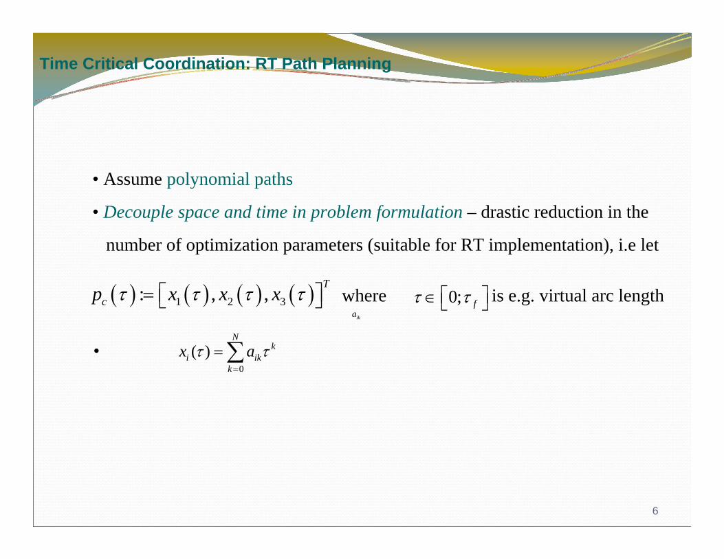
• Assume polynomial paths

• Decouple space and time in problem formulation – drastic reduction in the

number of optimization parameters (suitable for RT implementation), i.e let

( ) ( ) ( ) ( )1 2 3: , ,T

cp x x xτ τ τ τ= ⎡ ⎤⎣ ⎦ 0; fτ τ⎡ ⎤∈ ⎣ ⎦

0

( )N

ki ik

k

x aτ τ=

= ∑

where is e.g. virtual arc length

7Impact of changing total

path lengthImpact of changing total path length and initial jerk


8

,

-3000 -2000 -1000 0 1000 2000 3000 4000 50000

500

1000

1500

2000

2500

3000

3500

4000

x(m)

y(m

)

UAV 1

UAV 2UAV 3

-20000

20004000

6000

0

1000

2000

3000

4000

5000

0

200

400

600

800

X(m)

Y(m)

Z(m)

UAV 1 UAV 2

UAV 3

• Deconfliction in space – sequentially assigned final conditions


• essentially a 2D solution

tf1 dt AM vmin v1 v2 v3 vmax dmin

235s .005s 48s 15 m/s 16m/s 21m/s 30.2m/s

35m/s 203m

9

,

• Multiple UAVs – simultaneous arrival (deconfliction in time)

-2000 -1000 0 1000 2000 3000 4000 50000

500

1000

1500

2000

2500

3000

3500

0 1000 2000 3000 4000 5000 6000 7000 8000 900010

15

20

25

30

35

Speed profiles0 50 100 150 200 250 300 350

0

500

1000

1500

2000

2500

3000

3500

distances


3D paths

In this case the paths intersect, but if each vehicle follows the nominal speed profile

they will maintain a minimum separation distance at all times – disturbance rejection

is addressed at the coordination level

tf = 324 sec, AM = 271 sec

10

UAV Path Following Concept

Objective: follow predefined spatial 3D pathspaths are time-independent:

decoupling between space and time = separation of 3D path and speedspeed can be used as an additional DOF for time coordination

Analogous to “Tunnel in the Sky” concept familiar to pilots of 3D path and speed profile following

Eliminate path following (both distance and attitude) errors using angular rates

Follow speed profile to keep the a/c within its dynamic limitations.

Solution: Adaptive augmentation without any modifications to commercial autopilotConventional solution – backstepping – requires modification of source code of A/PGlobal results – but cancels inner loop

Limitation: Traditional UAV AP is not designed to follow an aggressive 3D path.

Intuitive AnalogyIntuitive Analogy

System ArchitectureInner/Outer Loop Solution

11

Onboard PC104

Onboard A/P(Inner loop)


Pitch rate

Yaw ratecommands

TrajectoryGeneration

User Laptop

polynomial

path

Boundary conditions

L1 adaptivecontroller

UAV Path Following

12

Problem Geometry

F: Serret-Frenet frameW: wind frameI: inertial frame

desired trajectoryUAV speedflight path angleheading anglepath length

position of UAV in inertial frame

( )cp l

][ IIII zyxq =

)(tvγψτ

Inertial Frame {I}

zI

xI

yF

τP

Qv

qF

pc

qI

UAVUAV

xF(T)yF(N)

yI

zF(B)

z1

Desired pathto follow

Serret Serret –– FrenetFrenet

Frame {F}Frame {F}

3D Kinematics Equations

1

/ cos cos/ cos sin/ sin

0/ 1/ 0 cos

/

I

I

I

v

dx dt vdy dt vdz dt v

d dt qd dt r

d dt

γ ψγ ψ

ψ

γψ γτ τ

−

== −=

⎤⎡ ⎤ ⎡ ⎡ ⎤= ⎥⎢ ⎥ ⎢ ⎢ ⎥

⎣ ⎦ ⎣ ⎣ ⎦⎦=

Input:

v

qrτ

13

Path

q

Q

{I} : Inertial Frame

P{F} : Serret-Frenet Frame

s1

y1

Virtual Target

Key idea: use virtual target to determine desired location on the pathMinimize the distance from the UAV to the virtual target on the pathReduce the angle between the vehicle velocity vector and local tangent to the path

Virtual target’s motion – extra degree of freedom

UAV Path Following

14

Path

Q

{I} : Inertial Frame

P

UAV Path Following (cont.)

Control the evolution of the virtual target : added degree of freedom

15

Error Equations in Error Equations in FF

where

I

F

W,γ ψ

, ,e e eφ θ ψCoordinatesystems

- Euler angles from F to W

][ FFFF zyxq =

- difference between and in FIq )(τcp

Kinematics

, ,e e eφ θ ψ

Kinematics equations in Kinematics equations in II

/ (1 ( ) ) cos cos/ ( ( ) ( ) ) cos sin

: / ( ) sin/

( , , ) ( , )/

/

F v F e e

F v F F e e

e F v F e

ee e e

e

v

dx dt y vdy dt x z v

G dz dt y vd dt q

D t T td dt r

d dt

τ κ τ θ ψτ κ τ ζ τ θ ψζ τ τ θ

θθ ψ θ

ψτ τ

⎧⎪

= − − +⎪⎪ = − − +⎪

= = − −⎨⎪⎡ ⎤ ⎡ ⎤⎪ = +⎢ ⎥ ⎢ ⎥⎪ ⎣ ⎦⎣ ⎦⎪

=⎩

16

Kinematic Control Law

Desired shaping functions

Path following control laws

( )

( )

1

22

1

23

1

cos cossin sin

sin sincos

c

c

F e e

ee F

e

ee F e

e

K x vcu K z vccu K y vc

θθ θ θ

θ

ψψ ψ ψ

ψ

τ θ ψθ δθ δ δθ δ

ψ δψ δ θ δ

ψ δ

= +−

= − − + +−

−= − − − +

−

&

&

&

17

Kinematic Control Law

Path following kinematics

Path following controller

Exponentially stable



Exponentially stable Semiglobal result:true for all kinematic error states

initialized in arbitrary region Ω

[ ]Ty q r=

[ ]Tc c cy q r=

18

Degradation of Performance

Without adaptation:• Errors ≈ 50m• Poor perf. in windy

cond.

Poor performance



UAVAutopilot

cyy ≠

cy

y

19

Cascaded System

))()()(()( szsusGsy p +=

y

yxgxfx )()( +=&

xupG eG

pGu

Autopilot UAVy

Path FollowingKinematics

UAV withAutopilot

Conventional solution – backstepping – requires modification of source code of A/PGlobal results – but cancels inner loop

20

Problem Reformulation

UAV with autopilot



UAVAutopilot

Design objective

cyy ≠ )()()( sysMsy c=

( )( )

( ) ( ) ( ) ( )

( ) ( ) ( ) ( )q c q

r c r

q s G s q s z s

r s G s r s z s

= +

= +

( ) ( ) ( )( ) ( ) ( )

c

c

q s M s q sr s M s r s

≈≈

L1 Adaptivecontroller

[ ]Ty q r=

[ ]Tc c cy q r=

[ ] ?Tad ad ady q r= −

21

Path Following: Summary

The cascaded system is UUB

The UUB can be reduced via selection of the filter bandwidth and the reference system bandwidth

Reducing the UUB leads to reduced robustness

L1 guarantees that the region of attraction for kinematic errors does not change



UAVAutopilot

cyy ≠ )()()( sysMsy c=

L1 Adaptivecontroller

[ ]Ty q r=

[ ]Tc c cy q r=

[ ]Tad ad ady q r=

22

Hardware-in-the-Loop Simulation

CAN Bus

6DOF nonlinear

model of the UAV

23

• comparison: with and without adaptation

Hardware-in-the-Loop Simulation

Path following w/o L1adaptation

Path following with L1adaptation

Hardware ( Second Generation)Networked Aircraft

Airframe; Sig Rascal 1102.8 meter span, 8 kg26 cc gas engine2‐3 hour endurance15‐35 m/s velocity

Payload:Cannon G9 12Mp gimbaled CameraPC104 with Wave Relay Mesh cardPC104 for gimbal control and AP interface

ADL MSMT3SEG PELCO‐NET 350 video server

24

25

Flight Test Results: Path Following• no adaptation – effect of gain changes

Flight Test Results: Path Following

26

−200 0 200 400 600 800 1000 1200 1400

−600

−400

−200

0

200

400

600

800

1000

UAV1 I.C.

UAV1 Fin.C.

Y East [m]

X N

orth

[m]

CmdUAV

Wind 5-7 m/s

L1 ON

Feature Following using Path Following

27

Feature Selection

-120.788 -120.786 -120.784 -120.782 -120.78 -120.778 -120.776 -120.77435.721

35.722

35.723

35.724

35.725

35.726

35.727

35.728

35.729

35.73

Desired Trajectory Generation

X - Long

Y - L

at

Resulting Mosaic usingOverlaid G9 images

Google Earth Overlay

28

,

Time-Critical Coordinated Motion Control

UAVs : initial positions

Target positions

UAVs must arrive at the same time; absolute time is not a priority!

29

,


Paths parameterized by length (τ=l)

- length of path for vehicle i

- time of arrival (unknown)

( ) ( ) / ; ( ) 1, i

i

i i i

f

f

f i f f f

l

t

l t l t l l t′ ′= = ∀

1fl

2fl

3fl

,

21fl′ =

11fl′ =

31fl′ =

Coordinated Path Following

PATHS (HIGHWAYS TO BE FOLLOWED)

Initial configuration

Reach (in-line) FORMATION at a

desired speed

dv !

Divide to Conquer ApproachIN-LINE FORMATION

Each vehicle runs its own PATH FOLLOWING

controller to steer itself to the path

Vehicles TALK and adjust theirSPEEDS in order to COORDINATE

themselves (reach formation)

Coordination error

Coordination error(in-line formation):

Normalized Path lengths and

Coordination state / error

2l′

1l′

12 1 2l l l′ ′ ′= −

12l′

1l′ 2l′

Communication Constraints

What is the communications topology? (GRAPH)

Non-bidirectional linksdirected graphs

Bidirectional Linksundirected graphs

vehicle

link

R. Murray [2002], B. Francis [2003], A. Jadbabaie [2003]

Communication Constraints

Communication Delays

Temporary Loss of Comms

Switching Comms Topology

Asynchronous Comms

Links with Networked Control and Estimation Theory

- set of vehicles that vehicle i communicates with

iJ

Communication ConstraintsV1

V2

V3

Node

edge

AdjacencyMatrix A =

1 1

1

1

0

0

V1 receives info from neighbours V2 and V3

V2 receives info from neighbour V1

V3 receives info from neighbour V1

DegreeMatrix D =

02

0

0

1 0

0 0 1

0

0

0

Communication ConstraintsV1

V2

V3

Node

edge

Neighbour set 1={ V2 , V3}

Neighbour set 2={ V1}

Neighbour set 3={ V1}

Laplacian

1 1 2 1 3

2 2 1

3 3 1

2 1 11 1 01 0 1

( ) ( )

L D A

l l l l lL l l l

l l l

− −⎛ ⎞⎜ ⎟= − = −⎜ ⎟⎜ ⎟−⎝ ⎠

′ ′ ′ ′ ′− + −⎛ ⎞ ⎛ ⎞⎜ ⎟ ⎜ ⎟′ ′ ′= −⎜ ⎟ ⎜ ⎟⎜ ⎟ ⎜ ⎟′ ′ ′−⎝ ⎠ ⎝ ⎠

--Graph is connected

Properties:

1 0L =rank 1 2L n⇒ = − =

1 2 30Ll l l l′ ′ ′ ′= ⇒ = =

Switching Communications:brief connectivity losses

V1

V2

V3

connected

V1

V3

disconnected

V1

V2

V3

connectedtime

1 2 31, 1, 0p p p= = =

1p

2p

1 2 31, 0, 1p p p= = =

3p

1p

1 2 30, 1, 0p p p= = =

2p

is a function of p, denoted pLL

Switching Communications:“uniformly” connected in mean

time

V1

V2

V3

1 2 31, 0, 0p p p= = =

1p V1

V2

V3

1 2 31, 0, 1p p p= = =

3p

V1

V3

1 2 30, 0, 0p p p= = =

1pL2pL

3pL

1 2 3[ , ]t t T p p pL L L L+ = + + [ , ]

[ , ]

rank 1 21 0

t t T

t t T

L nL

+

+

= − =⎧⇒ ⎨ =⎩

the union graph over time interval T

is connected


Coordination Control Law

1 . ./ cos cosi F i i e i e idl dt x vκ θ ψ= +Remember from Path Following

Adjust at the Coordination Level!


Coordination Control LawSpeed Asssignment

Integral term

Communications Topology


Key results (example)

11 ( ) , t 0, xt T T T n

tx QL Q x d R

Tτ τ μ

+ −≥ ∀ ≥ ∀ ∈∫

Suppose the Graph satisfies

some T, 0for μ >(graph does not even have to be connected at any time!)

“sensible” performance of the completePath Following + Coordination Controllers


A function of normalized path lengths

An ISS-like result

Time-Critical Coordinated Motion Control (HIL)

Coordinated Control of Multiple UAVs: Theoretical Framework / Practice

44

coordination

variables

Onboard A/P+ UAV

(Inner loop)


Pitch rate

Yaw ratecommands

Coordination Velocity

command

desired

path

L1 adaptation

PathGeneration

Network

L1 adaptation

Conclusion

NPSNPS: I. Kaminer, V. Dobrokhodov: I. Kaminer, V. DobrokhodovISTIST: A. Pascoal, A. Aguiar, R. Ghabcheloo : A. Pascoal, A. Aguiar, R. Ghabcheloo VPIVPI: N. Hovakimyan, E. Xargay, C. Cao: N. Hovakimyan, E. Xargay, C. Cao

The 17th IFAC World CongressJuly 6-11, 2008, Seoul, Korea

nps: i. kaminer, v. dobrokhodov ist: a. pascoal, a. aguiar...

Documents