National Renewable Energy Laboratory Innovation for Our Energy Future

A national laboratory of the U.S. Department of EnergyOffice of Energy Efficiency & Renewable Energy

NREL is operated by Midwest Research Institute ● Battelle Contract No. DE-AC36-99-GO10337

Model Validation at the 204 MW New Mexico Wind Energy Center Preprint E. Muljadi and C.P. Butterfield National Renewable Energy Laboratory

A. Ellis and J. Mechenbier Public Service Company of New Mexico

J. Hochheimer and R. Young FPL Energy LLC

N. Miller and R. Delmerico General Electric International, Inc.

R. Zavadil and J.C. Smith Utility Wind Interest Group

To be presented at the American Wind Energy Association WindPower 2006 Conference Pittsburgh, Pennsylvania June 4–7, 2006

Conference Paper NREL/CP-500-39048 June 2006

NOTICE

The submitted manuscript has been offered by an employee of the Midwest Research Institute (MRI), a contractor of the US Government under Contract No. DE-AC36-99GO10337. Accordingly, the US Government and MRI retain a nonexclusive royalty-free license to publish or reproduce the published form of this contribution, or allow others to do so, for US Government purposes.

This report was prepared as an account of work sponsored by an agency of the United States government. Neither the United States government nor any agency thereof, nor any of their employees, makes any warranty, express or implied, or assumes any legal liability or responsibility for the accuracy, completeness, or usefulness of any information, apparatus, product, or process disclosed, or represents that its use would not infringe privately owned rights. Reference herein to any specific commercial product, process, or service by trade name, trademark, manufacturer, or otherwise does not necessarily constitute or imply its endorsement, recommendation, or favoring by the United States government or any agency thereof. The views and opinions of authors expressed herein do not necessarily state or reflect those of the United States government or any agency thereof.

Available electronically at http://www.osti.gov/bridge

Available for a processing fee to U.S. Department of Energy and its contractors, in paper, from:

U.S. Department of Energy Office of Scientific and Technical Information P.O. Box 62 Oak Ridge, TN 37831-0062 phone: 865.576.8401 fax: 865.576.5728 email: mailto:reports@adonis.osti.gov

Available for sale to the public, in paper, from: U.S. Department of Commerce National Technical Information Service 5285 Port Royal Road Springfield, VA 22161 phone: 800.553.6847 fax: 703.605.6900 email: orders@ntis.fedworld.gov online ordering: http://www.ntis.gov/ordering.htm

Printed on paper containing at least 50% wastepaper, including 20% postconsumer waste

Model Validation at the 204 MW New Mexico Wind Energy Center

A. Ellis J. Mechenbier Public Service of New Mexico

Alvarado Square, MS 0604 Albuquerque NM 87104

E. Muljadi C.P. Butterfield National Renewable Energy Laboratory

1617 Cole Blvd Golden, CO 80401

J. Hochheimer R. Young FPL Energy LLC

700 Universe Blvd. Juno Beach, FL 33408

N. Miller R.Delmerico General Electric International, Inc.

1 River Road, Bldg. 2-605 Schenectady, New York 12345

R. Zavadil J.C.Smith Utility Wind Interest Group

2004 Lakebreeze Way Reston, VA 20191

Abstract—Wind energy continues to be one of the

fastest growing technology sectors. This trend is expected to continue globally as we attempt to fulfill a growing electrical energy demand in an environmentally responsible manner. As the number of wind power plants continues to grow and the level of penetration reaches high levels in some areas, there is an increased interest on the part of power system planners in methodologies and techniques that can be used to adequately represent wind power plants in the interconnected power systems.

Wind power plants can be very large in terms of installed capacity. The number of turbines within a single wind power plant can be as high 200 turbines or more, and the collector system within the wind power plant can have several hundred miles of overhead and underground lines. It is not practical to model in detail all individual turbines and the collector system for simulations typically conducted by power system planners. To simplify, it is a common practice to represent the entire wind power plant with a small group of equivalent turbine generators or a single turbine generator. The question is how much can a model be simplified and still preserve its faithfulness?

In this presentation, we will describe methods to derive and validate equivalent models for a large wind farm. FPL Energy’s 204-MW New Mexico Wind Energy Center, which is interconnected to the Public Service Company of New Mexico (PNM) transmission system, was used as a case study. The methods described are applicable to any large wind power plant. We will illustrate how to derive a simplified single-machine equivalent model of a large wind power plant (which includes an equivalent collector system model), preserving the net steady state and dynamic behavior of the actual installation. We use steady state as well as the dynamic analysis to derive the equivalent model. To verify the derivations, we compare the steady state and dynamic performance of the equivalent model against a detailed model of the wind power plant, which contains all the wind turbine generators and associated collector system.

Index Terms—wind turbine, wind farm, wind power plant, wind energy, dynamic transient, aggregation, equivalence, collector system, distribution network, power systems renewable energy.

I. INTRODUCTION The Taiban Mesa wind power plant is the most technically advanced wind plant in the country today. Built in 2003, it employs the latest advances in variable speed machine technology, incorporating low voltage ride through capability and controllable reactive power output. The plant employs 1.5 MW variable speed machines manufactured by General Electric Company (GE), is owned and operated by FPL Energy, LLC (FPLE), and sells its entire output to Public Service Company of New Mexico (PNM), on whose transmission system it is interconnected. The interconnection of the Taiban Mesa plant overcame unique engineering technical challenges. Located in eastern New Mexico, the plant interconnection substation is tapped into a 223 mile 345 kV transmission line. One terminal of the line is at Albuquerque, N.M., while the other end connects to the Blackwater HVDC converter station in Clovis, NM. The Blackwater HVDC station interconnects the Western and Eastern Interconnections. During the plant design phase, two of the unique engineering challenges included: • Consideration for low-voltage ride-through for faults on the PNM 345 kV transmission system. Since the plant nameplate represents a significant fraction of the PNM control area load, loss of the plant in response to transmission network faults would pose a severe operating challenge. At the time however, the industry discussion of low-voltage ride through for wind turbines was just beginning, so there was little precedent upon which to base the engineering design. • The advanced turbines at the wind plant are capable of dynamic reactive power control and coordinated regulation of the interconnect bus voltage. There was concern about this autonomous system interacting with the HVDC converter station voltage control scheme, and detailed engineering studies were conducted prior to plant commissioning to investigate this potential.

1

Validated positive-sequential computer models (power flow and transient stability) for the Taiban Mesa wind plant are critical for PNM transmission studies given the potential for the Taiban Mesa to interact with and influence the PNM transmission network. PNM has accumulated significant operating experience with the Taiban Mesa wind power plant and has pro-actively worked to refine its planning models used in GE –Positive-Sequence Load Flow (PSLF) program. However, wind power plant modeling, particularly model validation, remains an area of concern for the industry in general. NREL, in cooperation with the Wind Plant Modeling and Interconnection User Group of the Utility Wind Interest Group, seeks cooperation with PNM, FPLE, and GE to conduct a model development and verification effort in order to advance the state of the art in the development and use of wind plant models for

power system applications ("Joint Study"). In the next few sections, we will present our work in progress up to this point. In section I we have presented the background of this work. In section II the Taiban Mesa wind power plant equivalent circuit derivation will be briefly discussed. In section III dynamic simulation with low voltage ride through will be presented. In section IV, single turbine representation will be discussed and in section V, the full system representation will be presented. The conclusion and summary of the work will be presented in Section VI.

II. TAIBAN MESA WIND POWER PLANT EQUIVALENT CIRCUIT

A. General overview and general assumption In this section the background of circuit simplification

Caliente

Artesia

Blackwater

Guadalupe

B-A

Norton

Ojo

San Juan

Four Corners

Springerville

Greenlee

West Mesa

Belen

Hernandez

Taos

Sandia

Socorro

Elephant Butte

Picacho

Hollywood

Alamogordo

Holloman AFB

Newman Diablo

Luna

Hidalgo

Dona Ana

Las Vegas

Storrie Lake Bravo Dome

Springer

York Canyon

Los Alamos

Algodones Santa Fe

Blue Water

Ambrosia

Bisti

Pillar

Shiprock

Amrad

HVDC tie

HVDC tie Moriarty

Willard

Arroyo

Deming

Phelps Dodge

McKinley Yah-tah-ey

PEGS

Central

Salopeck

Rio Grande

WECC PATH 48

345 kV230 kV115 kV

Bernardo

Black Lake

Taiban Mesa

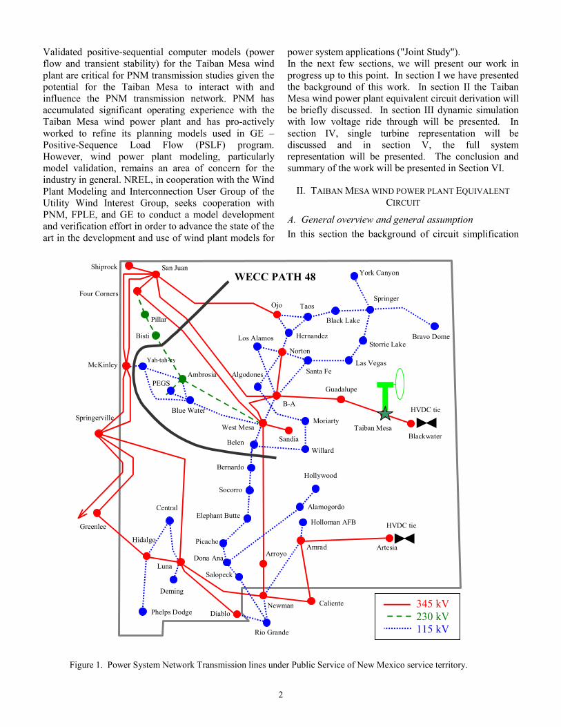
Figure 1. Power System Network Transmission lines under Public Service of New Mexico service territory.

2

will be described. Figure 1 shows the power system network transmission lines under Public Service of New Mexico service territory. Only the transmission level voltage interconnections were shown on the map. The Taiban Mesa wind power plant is indicated at a green star with label “Taiban Mesa” under the star. The wind power plant collector system consists of underground cables and overhead lines. The system distribution can be described by referring to Figure 2. It is shown here that the lowest level of grouping of the wind turbines is shown in blocks. In the planning stage, the power system designer will

compute the collector system requirement for the wind power plant. Normally, there are many considerations in placing the turbines on each site, which contributes to the diversity of impedances intra-turbines, and between the turbine and the substation transformer. Among many others, are, the wind resource of the site (micro siting strategy), the minimum distance between two turbines to avoid the turbulence wake caused by one turbine affecting another turbines, the voltage drop along the line feeders, the line losses within the collector system.

Taiban Mesa Infinite Bus

10999 345 kV

10995345 kV

1099834.5 kV

Each wind turbine generates a three-phase output power at 570 Volt at 60 Hz. This voltage is stepped up by a pad-mount-transformer to a higher voltage at 34.5 kV. A group of turbines (2 to 6 in a group) are connected together as a daisy chain connection at the high side of the pad mount transformer, and it is represented by a block shown in Figure 2. Figure 3 shows the content of each block where a string of turbines are connected in daisy chain fashion. The collector system data consists of intra-nodes impedances and line shunt capacitances in the wind power plants. From here, we have two choices to make. One is to simulate the entire wind power plant with each of the 136 turbines represented. Another one is to find an equivalent circuit representation of the 136 turbines. In simulating the entire wind power plant as a single turbine, we essentially observe the collective behavior predicted by a single turbine. Obviously, we loose some aspects of observation especially if the wind power plant is a very large one covering a very large area. There are two types of processes to be considered here for finding the equivalent circuit of a large wind power plant. The first one will be called Analytical Approach is based on the data of collector system provided by the power system designer. Another one will be called Deduction Approach deduced from load flow calculation of a complete full system representation (136 turbines).

B. Analytical approach At first, lets considered the analytical approach where the entire wind power plant can be considered as a single wind turbine. The final equivalent circuit representation of the entire 136 wind turbines is given in Figure 4. The equivalent of all the turbines and the collector

D2

D3

D4

D5

D1

D7

D8

D9

D10

D6

D15

D16

D14

D13

D12

D11

D23

D22

D19

D20

D18

D17

N8

D21

N3

N1 N2 N4 N6

N5 N7

Figure 2. Complete collector system in the wind farm.

D1

Figure 3 a) single series daisy-chain physical diagram b) equivalent representation of circuit (a)

(a) (b)

34.5 kV 345kV10998 10995

(0.01345 + j0.0497) B= -j 0.1004

10999Wind Farm

(0.002+j0.002)

Taiban MesaInfinite Bus

10997 109960.570 kV 34.5kV

(0.0014+j0.0828)

(0.0026 + j0.0245)

Figure 4. A single turbine equivalent circuit of Taiban Mesa wind farm.

3

system infrastructure within the wind power plant can be approached using power line losses equivalence. Detailed of this approach is described in paper reference [1], (paper submitted to the IEEE-PES 2006). The process of equivalencing the Taiban Mesa wind power plant is started from the lowest level of turbine connections (daisy-chain connected turbines). The equivalent circuit of these turbines (as shown in Figure 2) is represented as D1 through D23. First find the equivalent circuit of the block (e.g. D1 through D23). This simplification process converts the daisy chained wind turbines into a single impedance representation. Then the next step is to find the equivalent circuit of the parallel D1, D2, D3, D4, and D5 connected to N1. The same process is followed for the rest of the wind power plant collector system. And then we find the equivalent circuit of the parallel impedances connected to N1 through N8. Finally, the collector system of the wind power plant can be represented by the single line diagram shown in Figure 4.

C. Deduction approach In this approach, the entire 136 turbines are modeled in the load flow analysis. The load flow calculation is performed for the base case scenario. The real power loss, reactive power loss, and the currents in the branches are calculated by load flow and available in tabular form. The total loss in all of those branches within the collector system is then added. From the total loss and the main line current, we can find the equivalent impedance. From here, the equivalent impedance of the distribution power system network can be deduced. The shunt admittance is difficult to separate in the calculation of reactive power loss, however, we can use the same techniques developed in the previous section to find the approximate value of B.

Table 1. Equivalent Circuit of Collector system

Impedance-Shunt AdmittanceCircuit Representation R X B

Analytical 0.01345 0.0497 0.1004 Deduction 0.0104 0.0388 0.1004

A comparison between the results from the analytical approach and the result from the deduction approach are tabulated in Table 1. It is shown that the result from the two approaches is in a good agreement. The small difference between the two concepts is caused by the fact that in the analytical approach the output currents of the wind turbines are assumed to be identical, while in reality, due to the differences in the impedances, the phasor currents are not identical. With identical currents the sum of the currents at any summing junction will be maximized, and so will the total losses.

III. DYNAMIC SIMULATION WITH LVRT VOLTAGE PROFILE FOR MODEL VALIDATION

A. General Description To check the validity of model equivalencing, we use dynamic simulation. Based on the same transient condition, the two systems Single Turbine Representation (STR) and the Full System Representation (FTR) of 136 turbines are compred. In the next few sections we attempted to recreate a fictitious fault at the Taiban Mesa 345kV substation using a guidelines provided by AWEA. According to the AWEA-LVRT, the wind power plant must be connected to the grid as long as the voltage at the point of interconnection is at or above the specified voltage profile. The voltage profile starts at 1.0 p.u. at t = 0 and drops to 0.15 p.u. at t = 625 msecs, and the voltage slowly ramps up to 0.9 p.u. at t = 3.0 secs. The wind turbine must be connected indefinitely as the voltage drops down to 0.9 p.u. The low voltage ride through voltage profile provided can be shown in Figure 5. This

Figure 5. Test Voltage Profile (Ref. From FERC NOPR Jan 24, 2005)

10999 Taiban Mesa 345 kV

Full System Representation or

Single Turbine Representation

10995 345 kV Taiban Mesa

10998 34.5 kV Taiban Mesa

Figure 6. Single line diagram of the wind farm for two types of collector system configuration.

4

voltage profile is proposed by AWEA as appear in the FERC NOPR January 24, 2005. The purpose of applying this voltage profile is more to test the wind turbine behavior than to test the power system integrity. Under normal circumstances, this type of fault will be cleared within 4-5 normal clearing cycles.

Voltage

Since the relay protection of most of generators installed in the field is not set to survive this voltage profile, we will temporarily disable the protection systems for under/over voltage protection and under/over frequency protection. The voltage profile is applied at Taiban Mesa substation by using a generator classic (GNCLS) PSLF model with a voltage profile readable from an input file. This LVRT requirement does not consider frequency changes, thus, only the voltage magnitude is modulated according to this voltage profile shown.

Real power

B. Circuit Representation Reactive power The power system network can be simplified and it is shown in Figure 6. The single turbine representation is a wind power plant representation, where, all of the 136 wind turbines are represented by a single turbine. The equivalencing process is described in Section II. In Figure 6, the equivalent circuit to replace the CDNC block is shown in Figure 4 for a single turbine representation, or, it can be replaced by the circuit shown in Figure 2 for the full system representation.

Figure 7. Voltage, real power and reactive power response to the fault at the Taiban Mesa 345 kV.

IV. SINGLE TURBINE REPRESENTATION (STR)

A. Bus 10999 (Taiban Mesa –345 kV) Figure 7 shows the result of the simulation. The voltage profile representing a fictitious fault based on AWEA – LVRT proposed voltage profile is shown. The real power and reactive power traces are also shown on the same figure. The direction of the power flows shown in this figure is Taiban Mesa to the wind power plant, thus the actual flows from the wind power plant to Taiban Mesa is the mirror image of the traces shown.

B. Bus 10701 (Wind Turbine – 0.57 kV) Figure 8 shows the traces of voltage, real power, and reactive power output of the wind turbines represented by a single turbine. Since this simple circuit is a single series circuit connecting the wind turbine and Taiban Mesa substation, the traces shown in Figure 7 and Figure 8 are very similar with the exception of the collector system power loss. This point of measurement is the wind turbine terminals connected to the utility at the low voltage side. By looking at the range of the variables plotted, the voltage range is between 0.23 pu to 1.03 pu. The terminal voltage shows a second swing after the fault. Note, that although the voltage at the fault (Taiban Mesa

substation) goes down to 0.15 pu, but the impedance between the fault and the wind turbine terminals is sufficient as such that the lowest voltage during the fault, at the turbine terminals is about 10% higher. This is due to the voltage drops along the lines between the wind power plant and the substation. The turbine is able to

Voltage

Real power

Reactive power

Figure 8. Voltage, real power and reactive power response to the fault at the wind turbine terminals.

5

correct the voltage in the post fault condition although the voltage at Taiban Mesa substation stays at 0.9 p.u. The real power output of the wind turbine drops to –35.68 MW for a short period of time, and in the upswing, it reaches 228.49 MW. Note that this very short transient indicates the changes of the phasors voltages and currents with respect to the reference. While the current limit of the power converter is controlled very strictly, the voltage phase shift during transient is not controllable. During transient, the phase angle changes can create an impression as if the power (real or reactive) limit is exceeded. The post-fault (steady state) condition of the real power returns the terminal voltage, and output power (real and reactive) to the same level as its pre-fault condition, as expected. Note, that both the real and reactive power output of the wind turbine is the mirror image of the real and reactive power shown at the Table Mesa. The reactive power, in an attempt to regulate the voltage during the fault, it shows the correct trend, and the turbine produces reactive power that swings between 8.95 MVAR and 130.5 MVAR. It is also shown that the post-fault condition of the reactive power does not stay at the same level of output as the pre-fault condition due to the voltage at Taiban Mesa that stays at 0.9 pu indefinitely, three seconds after the fault occurs. Thus it is obvious that the reactive power trace reacts to the changes in voltage as planned. To observe the mechanical aspect of the turbine, the rotor speed, the pitch angle and the mechanical

(aerodynamic power) are shown in Figure 9. It is shown there that the speed fluctuates significantly creating the speed range between 1.0 pu and 1.26 pu. It is a bit difficult to predict the response of the rotor speed to this severe fault, because the speed variation is affected by both the mechanical and electrical systems. Electrical output torque is the restraining torque and the mechanical output torque is the driving torque. The electrical torque is affected by the available voltage at the turbine terminals and the output current (i.e. the power that can be generated) at any instant (including during the fault). The mechanical torque depends on the mechanical power and the rotor speed. The mechanical power variation is affected by the pitch angle of the blades, the rotational speed, and the wind speed itself at any moment. At any pitch angle, there is a valid Cp versus tip speed ratio applicable for solving aerodynamic power. And at any pitch angle, it is possible that the Cp goes to negative values when the tip speed ratio is too low or too high. The tip speed ratio, is the ratio of the tip speed with respect to the wind speed. Since the wind speed in this case study is assumed to be constant, the tip speed ratio is only affected by the rotor speed. It is interesting to note that the mechanical output variation goes between -1.1 p.u. (during the fault) to about 1.5 p.u. The pitch angle is controlled to maintain the rotor speed constant when the rotor speed reaches its rated speed. The pitch angle shown in Figure 9 varies significantly from low to high values with the swing of about 25 degrees. All in all, even with this severe fault, the turbine does not go into run-away condition, and the rotor speed is still controllable. Note, how the pitch angle variation has strongly affects the mechanical power output.

Rotor speed

Mechanical power

Pitch angle

Figure 9. Rotor speed, mechanical power and pitch angle variation pre-fault and post-fault condition.

C. Frequency comparison among Buses In Figure 10, the frequency of several buses are shown. Although in steady state the frequency is more or less constant, instantaneously, the frequency is proportional to the rate of change of the phase angle of the voltage phasor at the buses. The frequency at the Taiban Mesa (10999) and the frequency at the HV of the substation transformer (10995), have a similar trend because the impedance between the two buses is very small. There is a significant difference between the frequency of bus 10995 and bus 10998 (LV of the substation transformer). Although the two buses are separated by the leakage inductance of substation transformer, however the impedance of the transformer is significantly larger than the impedance of other components in the power system network under consideration. Also, note that the nature of the voltage variations (rate of change, control methods etc.) affect the frequency difference. As mentioned before, the bus voltage at Taiban Mesa (10999) is controlled by preset voltage profile, while the bus 10998

6

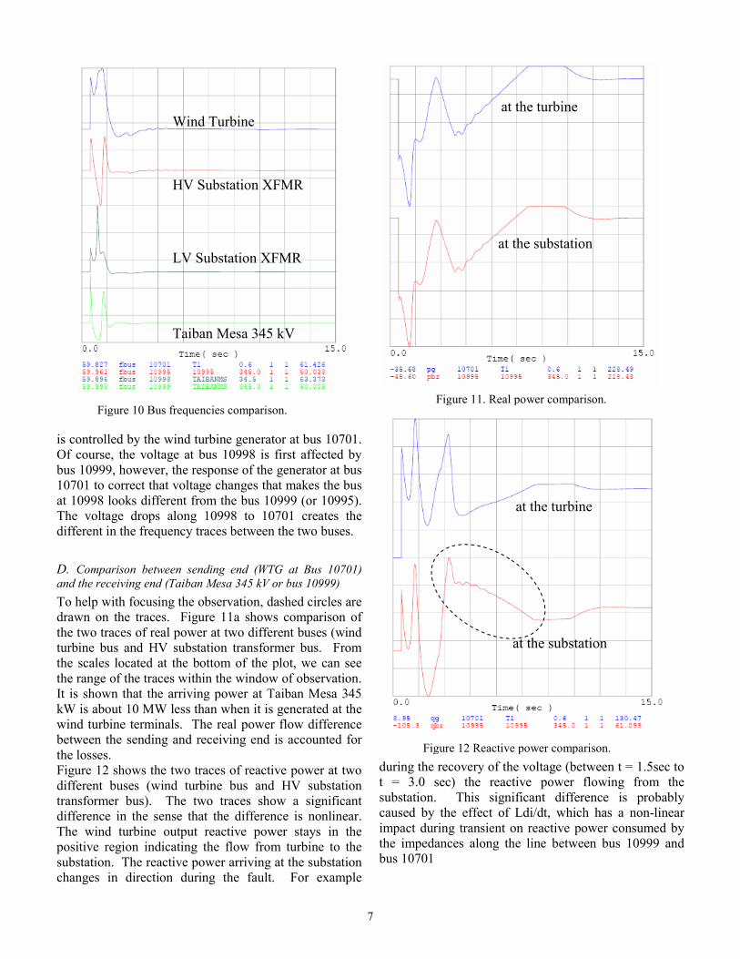
is controlled by the wind turbine generator at bus 10701. Of course, the voltage at bus 10998 is first affected by bus 10999, however, the response of the generator at bus 10701 to correct that voltage changes that makes the bus at 10998 looks different from the bus 10999 (or 10995). The voltage drops along 10998 to 10701 creates the different in the frequency traces between the two buses.

D. Comparison between sending end (WTG at Bus 10701) and the receiving end (Taiban Mesa 345 kV or bus 10999) To help with focusing the observation, dashed circles are drawn on the traces. Figure 11a shows comparison of the two traces of real power at two different buses (wind turbine bus and HV substation transformer bus. From the scales located at the bottom of the plot, we can see the range of the traces within the window of observation. It is shown that the arriving power at Taiban Mesa 345 kW is about 10 MW less than when it is generated at the wind turbine terminals. The real power flow difference between the sending and receiving end is accounted for the losses. Figure 12 shows the two traces of reactive power at two different buses (wind turbine bus and HV substation transformer bus). The two traces show a significant difference in the sense that the difference is nonlinear. The wind turbine output reactive power stays in the positive region indicating the flow from turbine to the substation. The reactive power arriving at the substation changes in direction during the fault. For example

during the recovery of the voltage (between t = 1.5sec to t = 3.0 sec) the reactive power flowing from the substation. This significant difference is probably caused by the effect of Ldi/dt, which has a non-linear impact during transient on reactive power consumed by the impedances along the line between bus 10999 and bus 10701

at the turbine Wind Turbine

HV Substation XFMR

at the substation LV Substation XFMR

Taiban Mesa 345 kV

Figure 11. Real power comparison. Figure 10 Bus frequencies comparison.

at the turbine

at the substation

Figure 12 Reactive power comparison.

7

V. FULL SYSTEM REPRESENTATION (FSR)

A. General Description In this section, the entire wind power plant is represented. Each turbine, each line connecting turbine to turbine, each pad mount transformer are represented. The same fault condition applied to the STR, is also applied to this FSR. The fault is applied to the same bus Taiban Mesa 345 kV (10999) by generating the voltage profile as in the single turbine equivalent. The same setting is applied to the relay protection to disable them during this simulation. From the simulation results, we can observe the behavior of individual turbines as well as the collective behavior of the entire wind power plant. The dynamic model of each generator consists of the wind turbine prime mover model, the generator-power converter model, and the relay protection model must each be represented in the dynamic file. Thus for the entire 136 turbines, these models must be repeated and represented creating many variables that must be computed at each time step. One disadvantage of representing all the turbines installed in the wind power plant is the computing time can be very long. B. Bus 10999 (Taiban Mesa 345 kV): At the pre-fault condition, there is a 204MW wind power generation from the wind power plant. When the fault occurs, the severity of the fault shows how the power flow is affected. Figure 13a illustrates the behavior of the voltage, real and reactive power at bus 10999

(Taiban Mesa Substation) when subjected to a voltage profile (AWEA-LVRT). For an easy comparison between FSR and STR, Figure 13b is brought here from the previous section (at the right hand side). The voltage waveform is the same preset voltage read from an input file. From Figure 13a, it is shown that the traces for real and reactive power for an FSR is rounder or smoother than the traces for the STR, indicating that there is some cancellation effect among the 136 turbines. Note that in the FSR, the wind speed driving each turbine is the same, thus the only diversity considered here is the impedance of the collector system. The range of variation of real power for an FSR is narrower than the range of variation for an STR. Table 2 is used to compare the range of real and reactive power variations.

TABLE 2. Power flow at bus 10999 for an FSR and STR FSR STR Max Min Max Min.

Real Power (MW) 13 -218 46 -217

Reactive Power (MVAR) 65 -60 107 -62

From this table, we can see that the use of STR assumes that all turbines respond instantaneously and are in sync with the rest of the turbines in the wind power plant, thus there is no cancellation or no smoothing effect in place. Sharp rise of high ramp rates is amplified by 136 times. On the other hands, for FSR, the diversity in the wind

Voltage Voltage

Real power Real power

Reactive power Reactive power

(a) Full System Representation (136 WTGs) (b) Single Turbine Representation

Figure 13. Voltage, real power and reactive power at Bus 10999.

8

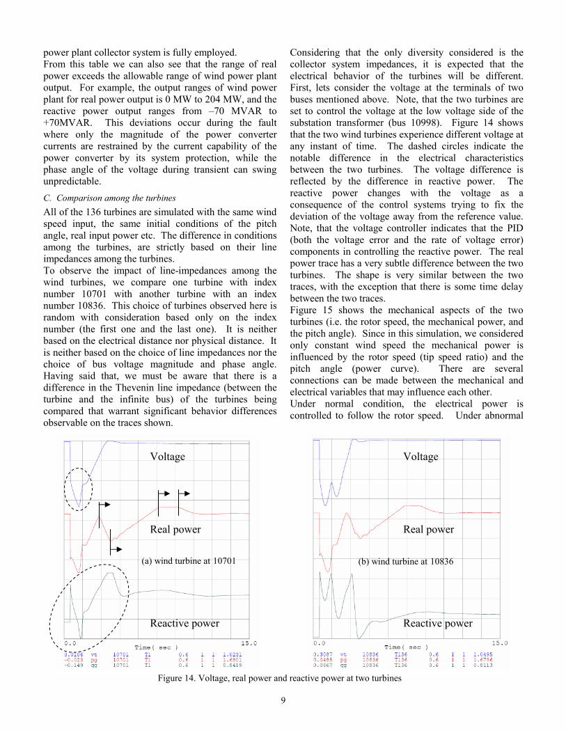
power plant collector system is fully employed. From this table we can also see that the range of real power exceeds the allowable range of wind power plant output. For example, the output ranges of wind power plant for real power output is 0 MW to 204 MW, and the reactive power output ranges from –70 MVAR to +70MVAR. This deviations occur during the fault where only the magnitude of the power converter currents are restrained by the current capability of the power converter by its system protection, while the phase angle of the voltage during transient can swing unpredictable. C. Comparison among the turbines All of the 136 turbines are simulated with the same wind speed input, the same initial conditions of the pitch angle, real input power etc. The difference in conditions among the turbines, are strictly based on their line impedances among the turbines. To observe the impact of line-impedances among the wind turbines, we compare one turbine with index number 10701 with another turbine with an index number 10836. This choice of turbines observed here is random with consideration based only on the index number (the first one and the last one). It is neither based on the electrical distance nor physical distance. It is neither based on the choice of line impedances nor the choice of bus voltage magnitude and phase angle. Having said that, we must be aware that there is a difference in the Thevenin line impedance (between the turbine and the infinite bus) of the turbines being compared that warrant significant behavior differences observable on the traces shown.

Considering that the only diversity considered is the collector system impedances, it is expected that the electrical behavior of the turbines will be different. First, lets consider the voltage at the terminals of two buses mentioned above. Note, that the two turbines are set to control the voltage at the low voltage side of the substation transformer (bus 10998). Figure 14 shows that the two wind turbines experience different voltage at any instant of time. The dashed circles indicate the notable difference in the electrical characteristics between the two turbines. The voltage difference is reflected by the difference in reactive power. The reactive power changes with the voltage as a consequence of the control systems trying to fix the deviation of the voltage away from the reference value. Note, that the voltage controller indicates that the PID (both the voltage error and the rate of voltage error) components in controlling the reactive power. The real power trace has a very subtle difference between the two turbines. The shape is very similar between the two traces, with the exception that there is some time delay between the two traces. Figure 15 shows the mechanical aspects of the two turbines (i.e. the rotor speed, the mechanical power, and the pitch angle). Since in this simulation, we considered only constant wind speed the mechanical power is influenced by the rotor speed (tip speed ratio) and the pitch angle (power curve). There are several connections can be made between the mechanical and electrical variables that may influence each other. Under normal condition, the electrical power is controlled to follow the rotor speed. Under abnormal

Voltage Voltage

Real power Real power

(a) wind turbine at 10701 (b) wind turbine at 10836

Reactive power Reactive power

Figure 14. Voltage, real power and reactive power at two turbines

9

conditions (fault, under voltage), the output power is affected by the available voltage at the grid and the current capability of the converter. Rotor speed depends on the balanced between the input mechanical power and electrical power. Rotor speed influences the mechanical driving (aerodynamic) power of the turbine and in addition, the blade pitch angle also influence the mechanical power. Once the balance of electrical and mechanical power is disturbed (fault, changes in blade pitch), the rotor speed will respond accordingly. Thus, there is a strong interaction between electrical and mechanical characteristics within a single turbine. Let us observe the wind turbine at bus 10701 alone. We can observe the interaction within turbine shown. When there is a fault on the electrical lines, the voltage drops significantly, the electrical output power drops significantly, the balanced of mechanical and electrical power is disturbed. The rotor speed changes with this balance. The rotor speed changes is further complicated by the fact that the shaft and dual inertia of the wind turbine and generator interacts to produce the rotor speed shown in Figure 15. As the rotor speed changes, the blade pitch mechanism becomes active to keep the rotor speed stabilized. The combination of electrical-mechanical balance, the shaft stiffness, the blade pitch action, all of them creates the total and final response of the rotor speed. Lets compare the mechanical aspects of the two turbines (Figure 15a and Figure 15b). With a known constant wind speed and relatively constant rotor speed, it is easy to relate the relationship between the pitch angle and

mechanical power. The mechanical power is shown mainly as a response to the pitch angle. Increase pitch angle means decrease in mechanical power, and decrease pitch angle means an increase in mechanical power. The control of pitch angle is an attempt to keep the rotor speed constant.

Rotor speed Rotor speed

Mechanical power Mechanical power

(a) wind turbine at 10701 (b) wind turbine at 10836

Pitch angle Pitch angle

Figure 15. Rotor speed, mechanical power and pitch angle variations.

Comparing the mechanical power, the rotor speed, and the pitch angle between the two turbines are very similar both in the shape and in the magnitude. Some of the differences are shown in the area encircles by the dashed lines.

VI. CONCLUSION This paper describes methods of equivalencing

collector system in a large wind power plant. We simplified a wind power plant with a 136 wind turbines into a single turbine representation. There are two methods we use in the process of simplification from 136 turbines into single representation. The analytical approach is strictly based on circuit concepts. The deduction approach is based on deduction derived from load flow analysis. From the results, we conclude that both methods are very compatible especially the value of X/R.

The full system representation (FSR) and the single turbine representation (STR) are compared in dynamic. performance. To verify the resulting equivalent circuit, we compare the two different turbine representations by using dynamic analysis. A simple low voltage ride through (LVRT) voltage profile proposed by AWEA is used as a test case. Both system representations are

10

subject to this voltage profile and the responses are compared.

What we find advantageous to the STR is that we have the advantage of representing the entire wind farm as a simple single turbine. The dynamic model of the turbine can be represented as one set of turbine models (we need only three sub-models per turbine, rather than 3x136 sub-models for the entire 136 turbines). This type of simplification tends to be on the conservatives side, especially when the relay protection is included in the simulation run. Thus, if the there is a severe fault, the choice is only two, either the wind power plant is disconnected or the wind power plant stays connected.

With the FSR, the entire wind power plant is represented in detail. Thus the wind power plant diversity in the line impedances, relay protection setting, wind speed on each individual turbine can be represented. When severe fault occur, we can find out how many turbines will be disconnected from the grid and how many turbines will stay connected to the grid.

VII. ACKNOWLEDGMENT We acknowledge the support of the U.S. Department

of Energy. We also thank William Price from General Electric International Inc., for help and discussions during the development of this project.

VIII. REFERENCES [1] E. Muljadi, C.P. Butterfield, A.Ellis, J. Mechenbier, J.

Hochheimer, R. Young, N. Miller, R. Delmerico, R. Zabadil, J.C. Smith, ”Equivalencing the Collector System of a Large Wind Power Plant,” presented at the IEEE Power Engineering Society, General Meeting 2006, Montreal, Quebec, Canada, June 18-22, 2006.

[2] E.N. Henrichsen and P.J. Nolan, “Dynamic stability of wind turbine generators,” IEEE Trans. Power App. Syst., Vol. PAS-101, pp. 2640-2648, Aug. 1982.

[3] Y.A. Kazachov, J.W. Feltes, and R. Zavadil, “Modeling wind farms for power system stability studies,”Power Engineering Society General Meeting, 2003, IEEE, Vol. 3, July 2003.

[4] E. Muljadi, C.P. Butterfield, and V. Gevorgian, “The impact of the output power fluctuation of a wind farm on a power grid,” in Conference Record:Third International Workshop on Transmission Networks for Offshore Wind Farms, Royal Institute of Technology, Stockholm, Sweden, April 2002.

[5] E. Muljadi and C.P. Butterfield, “Dynamic Model for Wind Farm Power Systems,” Global Wind Power Conference, Chicago, Illinois, March/April 2004.

[6] IEC Standard 61 400-21: Measurement and Assessment of Power Quality of Grid Connected Wind Turbines, International Electrotechnical Commission.

11

F1147-E(12/2004)

REPORT DOCUMENTATION PAGE Form Approved OMB No. 0704-0188

The public reporting burden for this collection of information is estimated to average 1 hour per response, including the time for reviewing instructions, searching existing data sources, gathering and maintaining the data needed, and completing and reviewing the collection of information. Send comments regarding this burden estimate or any other aspect of this collection of information, including suggestions for reducing the burden, to Department of Defense, Executive Services and Communications Directorate (0704-0188). Respondents should be aware that notwithstanding any other provision of law, no person shall be subject to any penalty for failing to comply with a collection of information if it does not display a currently valid OMB control number. PLEASE DO NOT RETURN YOUR FORM TO THE ABOVE ORGANIZATION. 1. REPORT DATE (DD-MM-YYYY)

17-06-06 2. REPORT TYPE

conference paper 3. DATES COVERED (From - To)

June 4-7, 2006 5a. CONTRACT NUMBER

DE-AC36-99-GO10337

5b. GRANT NUMBER

4. TITLE AND SUBTITLE Model Validation at the 204 MW New Mexico Wind Energy Center: Preprint

5c. PROGRAM ELEMENT NUMBER

5d. PROJECT NUMBER NREL/CP-500-39048

5e. TASK NUMBER

6. AUTHOR(S) E. Muljadi, C.P. Butterfield, A. Ellis, J. Mechenbier, J. Hochhiemer, R. Young, N. Miller, R. Delmerico, R. Zavadil, and J.C. Smith

5f. WORK UNIT NUMBER

7. PERFORMING ORGANIZATION NAME(S) AND ADDRESS(ES) National Renewable Energy Laboratory 1617 Cole Blvd. Golden, CO 80401-3393

8. PERFORMING ORGANIZATION REPORT NUMBER NREL/CP-500-39048

10. SPONSOR/MONITOR'S ACRONYM(S) NREL

9. SPONSORING/MONITORING AGENCY NAME(S) AND ADDRESS(ES)

11. SPONSORING/MONITORING AGENCY REPORT NUMBER

12. DISTRIBUTION AVAILABILITY STATEMENT National Technical Information Service U.S. Department of Commerce 5285 Port Royal Road Springfield, VA 22161

13. SUPPLEMENTARY NOTES

14. ABSTRACT (Maximum 200 Words) In this paper, we describe methods to derive and validate equivalent models for a large wind farm. FPL Energy’s 204-MW New Mexico Wind Energy Center, which is interconnected to the Public Service Company of New Mexico (PNM) transmission system, was used as a case study. The methods described are applicable to any large wind power plant.

15. SUBJECT TERMS wind energy; wind farm; wind power plant; FPL Energy; New Mexico Wind Energy Center; wind farm model

16. SECURITY CLASSIFICATION OF: 19a. NAME OF RESPONSIBLE PERSON a. REPORT

Unclassified b. ABSTRACT Unclassified

c. THIS PAGE Unclassified

17. LIMITATION OF ABSTRACT

UL

18. NUMBER OF PAGES

19b. TELEPHONE NUMBER (Include area code)

Standard Form 298 (Rev. 8/98) Prescribed by ANSI Std. Z39.18