Nuclear Shutdown, Coal Power Generation, and Infant

Health: Evidence from the Tennessee Valley Authority

(TVA) in the 1980s⇤

Edson R. Severnini

†

First Version: May 2014

This version: August 2015

Abstract

When environmental regulations focus on a subset of power plants, the ultimate goal of

human health protection may not be reached. Because power plants are interconnected

through the electrical grid, excessive scrutiny of a group of facilities may generate more

pollution out of another group, with potential deleterious effects to public health. I

study the impact of the shutdown of nuclear power plants in the Tennessee Valley Au-

thority (TVA) in the 1980s, on health outcomes at birth. After the Three Mile Island

accident in 1979, the Nuclear Regulatory Commission (NRC) intensified inspections in

nuclear facilities leading to the shutdown of many of them, including Browns Ferry and

Sequoyah in the TVA area. I first show that, in response to the shutdown, electric-

ity generation shifts one-for-one to coal-fired power plants within TVA, increasing air

pollution in counties where they are located. Second, I find that babies born after the

shutdown have both lower birth weight and lower gestational age in the counties most

affected by the shutdown. Third, I highlight the presence of substantial heterogeneity

in those effects depending on how much more electricity those coal-powered facilities are

⇤I am very thankful to Reed Walker for invaluable detailed feedback on an earlier version of the paper, toAntonio Bento, David Card, Janet Currie, Michael Greenstone, Patrick Kline, Joshua Lewis, Tarso Madeira,Jesse Rothstein, Allison Shertzer and Lowell Taylor for very helpful suggestions, and seminar participantsat Cornell University, UC Berkeley-Labor Lunch, University of Montreal, 36th Meeting of the BrazilianEconometric Society, and the 2nd Economics of Low-Carbon Markets Conference for useful comments.

†Mailing address: Carnegie Mellon University, 4800 Forbes Ave, Pittsburgh, PA 15213Phone: (510) 860-1808Email: ersevernini@gmail.com

1

generating in response to the shutdown. Lastly, I use the heterogeneity in response to

the shutdown to provide suggestive evidence on the "safe" threshold of exposure to to-

tal suspended particles (TSP), which may help the Environmental Protection Agency

(EPA) to set the National Ambient Air Quality Standards (NAAQS) for particulate

matters (PM). It may also help regulators to incentivize power companies to respond

optimally to unexpected energy shortages.

Keywords: Nuclear Shutdown, Power Grid, Coal Power, Air Pollution, Birth Weight,

Gestational Age

1 Introduction

Nuclear accidents usually generate a tremendous drop in support for nuclear energy. The

Fukushima nuclear disaster in March 2011, for example, gave rise to a public backlash

against the nuclear power industry around the world. As a result of such a pressure, some

countries/states reacted promptly by enacting new regulations or by shutting down nuclear

facilities. Germany, for instance, started a nuclear phase-out right away1, permanently

shutting down eight of its seventeen reactors by August 2011, and pledging to close the rest

by the end of 2022. California followed suit by retiring the San Onofre Nuclear Generating

Station (SONGS) in June 2013. Although media outlets focus attention on damages to public

health potentially caused by exposure to high levels of radioactivity, news coverage misses

important aspects of the debate. Exceptionally, a recent New York Times editorial clearly

points out some of those missing elements: "Only Germany succumbed to panic after the

Fukushima disaster and began to phase out all nuclear power in favor of huge investments

in renewable sources like wind and sun. One consequence has been at least a temporary

increase in greenhouse emissions as Germany has been forced to fire up old coal- and gas-

powered plants. The dangers of nuclear power are real, but the accidents that have occurred,

even Chernobyl, do not compare to the damage to the earth being inflicted by the burning of

fossil fuels - coal, gas and oil." (May 1, 2014).1According to Goebel et al. (2013), support to nuclear energy dropped 20 percent in Germany after the

Fukushima disaster.

2

In this paper, I document the shift in electricity generation from nuclear to coal-fired

power plants after the shutdown of the nuclear facilities of the Tennessee Valley Authority

(TVA) in the 1980s, following the Three Mile Island accident in 1979, and provide evidence

of the resulting increase in air pollution and reduction in birth weight and gestational age

in the most affected counties. I show that these empirical findings are consistent with a

simple model where consumers value electricity, air quality and health, but power generation

damages air quality and health through emissions of pollutants and radioactivity. Also, I

use the heterogeneity in response to the nuclear shutdown by coal-powered plants within

the TVA power grid to shed light on the "safe" threshold of exposure to total suspended

particles (TSP), which may help the Environmental Protection Agency (EPA) to set the

National Ambient Air Quality Standards (NAAQS) for particulate matters (PM). It may

also help regulators to incentivize power companies to respond optimally to unexpected

energy shortages.

The Three Mile Island accident was a partial nuclear meltdown that occurred on March

28, 1979, in one of the two Three Mile Island nuclear reactors in Pennsylvania. Being the

worst accident in U.S. commercial nuclear power plant history, the accident crystallized

anti-nuclear safety concerns among activists and the general public. Following the public

backlash, the Nuclear Regulatory Comission (NRC) started cracking down on nuclear fa-

cilities, leading to new regulations and the shutdown of several nuclear plants around the

nation in the 1980s, including Browns Ferry and Sequoyah in the TVA area in 1985. I ex-

ploit this setting to study the substitution among energy sources in electricity generation,

and potential consequences of the use of non-renewable sources on air quality and public

health. I focus on the TVA because it has a diverse portfolio of power sources which are

connected through the electrical grid - hydroelectric dams, coal- and gas-fired plants, and

nuclear facilities -, and is self-sufficient in power generation. Hence, when an energy source

faces a temporary shock, responses are likely to occur within the area. Besides, the TVA

was operating the nation’s largest electric power system in 1985, the year of the nuclear

3

shutdown.

I first investigate whether environmental regulations targeted at a subset of power plants

in a network of energy production are effective at protecting public health. Chain reactions

within the power grid may completely offset the perceived health benefits of the nuclear

shutdown when the response is an increase in electricity generation through the burning of

fossil fuels. By plotting monthly electricity generation data at the plant-fuel level from the

Historic EIA-906 Form in figure 1, we can see that such pattern indeed emerges after the

shutdown of the TVA nuclear plants. By employing an empirical strategy similar to the

dynamic reduced-form approach advanced by Cullen (2013), I estimate those responses and

find out that the substitution between nuclear and coal seems to be one-for-one. That is,

each megawatt-hour not produced by nuclear power plants due to the shutdown appears to

be generated by coal-powered plants. Furthermore, summary statistics presented in the last

row of table 1 show that the nuclear shutdown leads to not only a shift in power generation to

coal-fired plants, but also an increase in TSP concentration, and a decrease in birth weight.

Monthly measures of TSP concentration were constructed by aggregating daily readings from

the network of monitoring stations provided by EPA. Natality data come from the National

Vital Statistics System of the National Center for Health Statistics (NCHS’s). Estimates

from the econometric analysis corroborate the broad picture just described, and I conclude

that targeted environmental regulations in network do not seem to protect public health.

Although the general results arising from the nuclear shutdown are already illuminating,

a more detailed analysis reveals a rich pattern of heterogeneity in the responses of interest.

By splitting the power generation response of coal-fired power plants into four groups - high,

medium, low, and negligible -, the right-hand side of table 1 indicates that TSP and birth

weight responses also differ across groups. To the best of my knowledge, this heterogeneity

driven by responses within the power grid has not been exploited in studies of air pollution,

but has the potential to enrich the analysis. In fact, a single shock can generate multiple

sources of variation in terms of pollution intensity and geographic areas. I take advantage of

4

such heterogeneity by employing a difference-in-differences approach to estimate the impact

of air pollution on birth weight and gestational age. I define the control group as the set of

counties whose coal-fired power plants were not affected by the nuclear shutdown - the ones

with negligible variation, and three treatment groups according to their pollution intensity.

The difference-in-differences approach exploiting the network heterogeneity allows me to

address my second research question: are there levels of TSP concentration that are "safe" to

infants? In a recent review of the literature on the impact of pollution on health outcomes,

Currie et al. (2014) point out the preponderance of evidence of harmful effects of high levels

of pollution, but emphasize the need to identify "safe" thresholds. This is a particularly

important question for policy because it could guide EPA in the process of setting the

NAAQS, for instance. It may also give regulators tools to incentivize power companies to

respond optimally to unexpected energy shortages.

In this attempt to recover the dose response function of pollution motivated by Currie et

al. (2014), notice that TSP concentrations displayed in the right-hand side of table 1 do not

appear to respond proportionally to power generation. Although the high group generates

around 30 percent more electricity than the medium group on average, TSP responses seem

to be very similar. In fact, the patterns depicted in figure 3 look a lot alike, with the only

difference being the level of pollution that they begin with. The medium group starts in

the 30s and jumps to the 40s µg/m3, while the high group moves from the 40s to the 50s

µg/m3. Just for reference, the EPA annual standard for TSP is 75 µg/m3 from 1971 to

1987. Difference-in-differences estimates reveal that even though TSP concentrations are

below EPA standards in 1985, they are not at "safe" levels. Air pollution seems to decrease

birth weight by roughly 134 grams, or 5.5 log points, when TSP concentration is above 50

µg/m3. No statistically significant effects are found for TSP levels below 50 µg/m3. Indeed,

these effects are evident even in the raw data as depicted by figure 3. Therefore, 50 µg/m3

appears to be a "safe" threshold. When translating these TSP concentrations into particulate

5

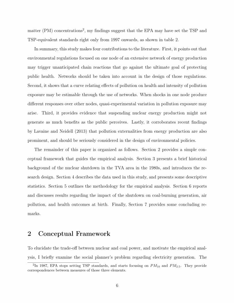
matter (PM) concentrations2, my findings suggest that the EPA may have set the TSP and

TSP-equivalent standards right only from 1997 onwards, as shown in table 2.

In summary, this study makes four contributions to the literature. First, it points out that

environmental regulations focused on one node of an extensive network of energy production

may trigger unanticipated chain reactions that go against the ultimate goal of protecting

public health. Networks should be taken into account in the design of those regulations.

Second, it shows that a curve relating effects of pollution on health and intensity of pollution

exposure may be estimable through the use of networks. When shocks in one node produce

different responses over other nodes, quasi-experimental variation in pollution exposure may

arise. Third, it provides evidence that suspending nuclear energy production might not

generate as much benefits as the public perceives. Lastly, it corroborates recent findings

by Lavaine and Neidell (2013) that pollution externalities from energy production are also

prominent, and should be seriously considered in the design of environmental policies.

The remainder of this paper is organized as follows. Section 2 provides a simple con-

ceptual framework that guides the empirical analysis. Section 3 presents a brief historical

background of the nuclear shutdown in the TVA area in the 1980s, and introduces the re-

search design. Section 4 describes the data used in this study, and presents some descriptive

statistics. Section 5 outlines the methodology for the empirical analysis. Section 6 reports

and discusses results regarding the impact of the shutdown on coal-burning generation, air

pollution, and health outcomes at birth. Finally, Section 7 provides some concluding re-

marks.

2 Conceptual Framework

To elucidate the trade-off between nuclear and coal power, and motivate the empirical anal-

ysis, I briefly examine the social planner’s problem regarding electricity generation. The2In 1987, EPA stops setting TSP standards, and starts focusing on PM10 and PM2.5. They provide

correspondences between measures of those three elements.

6

social planner maximizes the utility of a representative consumer over electricity, air quality,

and health, taking into account potential damages to air quality and health due to emissions

of pollutants and radioactivity arising from power generation.

2.1 Set-up

The social planner maximizes a concave utility function U(E,A,H) of a representative con-

sumer over electricity E, air quality A, and health H. Electricity is generated by a concave

production function E(C,N,R) separable in coal C, uranium N , and river water R3. That

is, electricity is generated by coal-fired power plants, nuc

lear facilities, and hydroelectric dams. Because coal-fired power plants emit lots of pol-

lutants, I assume that air quality is a nonincreasing function of coal. That is, A(C), with

AC 0. Finally, I assume that health is a nonincreasing function of air pollution and ra-

dioactivity released from nuclear reactors, i.e., H(A,N), with HA � 0 and HN 0. The

social planner’s problem can be expressed as

MaxC,N,R2R3+U(E,A,H)

s.t. E = E(C,N,R)

A = A(C)

H = H(A,N),

which is equivalent to

MaxC,N,R2R3+U(E(C,N,R), A(C), H(A(C), N)).

3One can also treat R as another source of renewable energy such as wind and solar.

7

The first order conditions (FOCs) for such a problem can be written as

UEEC + (UA + UHHA)AC = 0

UEEN + UHHN = 0

UEER > 0.

2.2 Model Predictions

This simple model provides three main predictions. First, the social planner operates power

plants with renewable sources of energy at full capacity before turning to coal and nuclear

power. In this context, hydroelectric dams should generate an important part of the baseload.

Second, once renewables are fully exploited, the trade-off between nuclear and coal power

could emerge. If environmental regulations are targeted at nuclear power plants, we should

expect a shift in electricity generation to coal-powered plants. The trade-off exists only if

the additional coal power generation deteriorates air quality. In the FOCs, only if AC is not

zero. If that is the case, the reduction in the risk of exposure to radioactivity through HN

could be offset by the increase in the exposure to air pollution. If regulations also constrain

emissions of existing coal-fired power plants such as the ones pushed by EPA recently, then

perhaps air quality would not be affected, and the trade-off would not emerge. Third, the

intensity of the trade-off depends on (i) potential nonlinearities in the effect of coal power

generation on air quality (ACC), (ii) the impact of air pollution on health (HA), and (iii)

potential nonlinearities in the relationship betwen pollution and health (HAA).

Recent studies have provided strong evidence of deleterious health effects of radioactivity

(Almond et al., 2009; Black et al., 2014). There is also plenty of evidence of the effects of

air pollution on health (Stieb et al., 2012; Currie et al., 2014). However, to the best of my

knowledge, there is no study linking the functioning of the electricity markets to non-market

outcomes such as air quality and health. Also, nonlinearities in health responses to pollution,

which would provide guidelines for policymaking such as setting the NAAQS by EPA, have

yet to be credibly estimated. I exploit the quasi-experimental design associated with the

8

nuclear shutdown in the TVA in the 1980s to shed light on those issues4.

3 Historical Background and Research Design

In order to investigate the trade-off between coal and nuclear power empirically, it would be

desirable to find exogenous variation in electricity generation by nuclear plants within a power

grid with a diverse portfolio of power plants. As will be described in the data section, the

TVA has a variety of large power plants, mainly hydroelectric dams, coal-powered plants,

and nuclear facilities. Thus, in the empirical analysis, I exploit the shutdown of nuclear

power plants in the TVA area in the 1980s as such an exogenous source of variation to

identify substitution between energy sources and its consequences to air pollution and health

outcomes. I now discuss some background information on such a nuclear shutdown in 1985.

Figure 4 depicts a timeline with important events.

As mentioned before, the Three Mile Island Unit 2 reactor partially melted down on

March 28, 1979, near Middletown, Pennsylvania. This was the most serious accident in

U.S. commercial nuclear power plant operating history. It triggered the NRC to tighten and

heighten its regulatory oversight, bringing about sweeping changes in many areas of nuclear

power plant operations.

Two months before the 1979 Three Mile Island nuclear accident, the Union of Concerned

Scientists (UCS) called upon the government to shut down the facility and 15 other nuclear

reactors, based on analysis showing that the NRC had dramatically understated the prob-

ability of an accident5. The public backlash that followed the accident forced the NRC to

crack down on nuclear facilities, leading to the shutdown of several nuclear reactors in the

1985 to 1990 time frame. The TVA Browns Ferry Units 1, 2 and 3, and Sequoyah Units 14Observe that the marginal utility of electricity enters every FOC directly. Although EPA designs and

implements regulations based on evidence of harm to the environment or public health, a proper cost-benefitanalysis should include the value of electricity to consumers. Indeed, Lewis and Severnini (2014) show thatelectricity is extremely valuable to farmers due to increases in productivity and household’s well-being.

5Ever since the Three Mile Island accident, federal, state, and local officials have looked to UCS forunbiased information about the safety of nuclear power plants.

9

and 2, as well as Davis-Besse, Fort St. Vrain, Nine Mile Point Unit 1, Peach Bottom Units

2 and 3, Pilgrim, Rancho Seco, and Surry Unit 2, all had year-plus outages in this period

(UCS, n.d.).

At Browns Ferry, NRC inspectors identified 652 violations between 1981 and 1984, and

the agency imposed $413,000 in fines (USC, n.d.). In July 1984, the NRC issued an order

requiring TVA to implement its Regulatory Performance Improvement Program (RPIP) and

provide periodic status reports. In February 1985, reactor vessel water level instrumentation

problems happened in Unit 3, leading TVA to cease operations in March 19 at all three

Browns Ferry units to focus on programmatic improvements. By September 1985, NRC

stated that the RPIP had been ineffective and required TVA to try again with another plan.

The shutdown of Browns Ferry would last for approximately five years.

Regarding Sequoyah, the NRC induced its outage based on new regulations taking effect

in March 1985. After the agency informed TVA that Sequoyah would be one of the first

plants to be audited according to the new requirements, the company brought in a contractor

to pre-audit the facility. That independent review indicated that reactors could not be safely

shut down in the event of an accident. Hence, TVA voluntarily ceased operations at both

reactors in August 22, 1985, before the NRC’s inspectors got a chance to do so (USC, n.d.).

That shutdown would last until November 1988.

The UCS clearly states that "[t]hese back-to-back outages reflect a regulatory bias first

identified by the various inquiries into the Three Mile Island Unit 2 accident and still not

exorcised." (UCS, n.d., Report on Browns Ferry Unit 3 - p.2). Therefore, the Three Mile

Island accident appears to have induced targeted environmental regulations. The nuclear

facilities were under much more scrutiny than the coal- and gas-powered plants in those years.

Furthermore, TVA annual reports indicate that the shutdown was unexpected. According

to the reports, TVA had an extraordinary perfomance in 1985 due to "unplanned reductions

in nuclear and hydro generation" (TVA, 1985, p.26).

The reductions in hydro mentioned in the TVA report resulted from an unusual drought

10

in the area during the 1980s, which limited the supply of its only source of renewable energy.

This short-run capacity constraint in renewables makes this setting even more appropriate to

examine the potential trade-off between coal and nuclear power. To some extent, the operator

may be forced to ramp up production in coal-fired power plants, which could increase air

pollution in the area, and perhaps deterioration of public health.

4 Data

The data I use in this study come from three sources. To investigate the response of TVA

hydro and coal-fired power plants to the shutdown of Browns Ferry and Sequoyah nuclear

facilities in 1985, I utilize monthly electricity generation data at the plant-fuel level from

the Historic EIA-906 Form. To obtain the impact of the nuclear shutdown on air pollution,

I construct monthly measures of TSP at the county level. Daily TSP readings from the

network of monitoring stations in the TVA area were provided by EPA under a Freedom of

Information Act (FOIA) request. To aggregate these daily readings into monthly measures,

I employ the same procedure used by EPA to produce its annual summaries. To estimate

the effect of the pollution arising from coal-fired power plants in response to the nuclear

shutdown on birthweight, I use natality data from the National Vital Statistics System of

the National Center for Health Statistics (NCHS’s). The NCHS’s birth data provide rich

demographic and health information of infants and their mothers. I focus my analysis in the

period 1983-1987, which covers eighteen months before and after the shutdown. Eighteen

months just represent two pregnancy cycles, which is a natural time frame when undertaking

the birth weight analysis.

The TVA was operating the nation’s largest electric power system, and had a pretty

diverse portfolio of power generation in 1985, the year of the nuclear shutdown. Focusing on

large plants - 100 megawatts of capacity or more -, the TVA had 15 hydroelectric dams, 11

coal-fired plants, and two nuclear facilities, as you can see in figure (5). The blue squares

11

represent hydro, the red circles coal, and the yellow triangles nuclear plants. Since hydro

dams do not seem to respond to the nuclear shutdown, I focus my analysis on coal-powered

plants. Figure (6) plots only those plants together with the nuclear generating stations. The

different symbols represent the heterogeneity in power generation responses to the nuclear

shutdown, as pointed out previously based on the summary statistics of table (1). The

red diamond represents the Paradise coal-fired plant, with the highest variation in power

generation due to the shutdown (H �4PG), the red square represents Cumberland, with

a medium response (M � 4PG), the red circles represent coal-powered plants with low

responses (L�4PG), and the red hollow circles represents facilities with negligible responses

(N �4PG)6.

With the exception of Allen Fossil Plant in the Memphis metropolitan area, all coal-

fired plants are located in counties with low population density, as you can notice from the

relatively small number of births in table (3). Observe that the high and medium groups are

made of only one power plant each, so in my main analysis I compare these two distinctive

counties with the group of counties with low responses, and with the control group. Recall

that the control group is defined as the group of counties whose responses of their coal-

powered plants to the nuclear shutdown are economically and statistically insignificant.

The sample for my birth weight analysis has almost 56,000 observations, as shown in table

(3). The middle panel in the table contains the information of plants used in my analysis.

I exclude Kingston and Bull Run coal-fired plants because they are located in neighboring

counties, and I have not found reliable information on wind patterns for that area in that

period of time, so I cannot control precisely for upwind pollution. The right-hand side panel

of that table includes those two plants. Later on, I show that my results are not sensitive to

the inclusion of those plants.

It is important to point out the difference in sample sizes for the counties hosting Paradise

and Cumberland. Because the number of births around Cumberland is much smaller than6In Appendix A, I provide evidence that most of the response in power generation can be explained by

cost considerations within TVA.

12

around Paradise, one should expect less precision for estimates associated with the medium

response group. A reweighting strategy based on number of births is used to check whether

the results are robust to such heterogeneity.

5 Empirical Strategy

In this section, I present the methodology to provide empirical evidence on the consequences

of the shutdown of the TVA nuclear facilities in the 1980s. Motivated by the predictions of the

model discussed in section (2), I address three main topics: (i) how power generation changes

after the shutdown both in hydro and coal-fired plants, (ii) how air pollution, measured as

TSP concentration, respond to the shutdown because of additional emissions by coal-powered

plants, and (iii) how birthweight is affected in counties where both power generation and air

pollution increase after the shutdown. Throghout my analysis

5.1 Response of Power Generation

In order to estimate the response of coal and hydro power generation to the nuclear shutdown,

I build on the approach advanced by Cullen (2013). Basically, I estimate the following

equations for each power source - coal versus hydro:

PGencm = �0 + �1cDNucShutm + Zcm� + �c + �m + ✓y + "cm, (1)

or PGencm = �0 + �1cPGenNucm + �2cPGenNucm�1 + Zcm� + �c + �m + ✓y + "cm, (2)

where c stands for county, m for month, and y for calendar year. PGen represents power

generation measured in megawatt-hours, PGenNuc is power generated by nuclear plants,

DNucShut represents a dummy variable that takes value one from the shutdown onwards,

and Z is a set control variables such as temperature and precipitation.

Notice that this approach accounts for dynamics in the production process. As discussed

13

in Cullen (2011), the operating decision of a coal-powered plant is inherently dynamic due to

costs associated with startup, shut down, and ramping up and down production. Therefore,

in the estimation one must include not only contemporaneous covariates, but also elements of

the information set which the electric utility - TVA, in this case - considers when adjusting its

optimal production. At the end of the day, the estimating equation recovers the reduced-form

optimal policy function coming from the dynamic programming problem of each generator,

taking into account firm’s expectations. For the sake of completeness, lagged variables are

also included in Z. In fact, Z contains a quadratic function of contemporaneous and lagged

precipitation and temperature.

The time frame of my analysis is eighteen months before and after the shutdown. It is

equivalent to two full-term pregnancies, and is less than the typical two years to construct

a coal-fired power plant. Because eighteen months are not enough for electric utilities to

adjust production by increasing capacity, the responses captured in �1c’s are in the intensive

margin. In this sense, the nuclear shutdown represents an exogenous source of variation in

power generation, since it can be seen as a shock to the other power plants.

Finally, I estimate equations (1) and (2) separately for counties with coal versus hydro

power plants. My underlying assumption is that TVA’s decision making may be different for

coal and hydro generation. In any case, the variables of interest are interacted with counties

so that responses can be obtained for each and every power plant.

5.2 Response of Air Pollution

Regarding the estimation of air pollution responses, I follow the approach developed for

responses of power generation. I just substitute TSP concentration for power generation as

the dependent variable in the estimating equations. That is,

TSPcm = �0 + �1cDNucShutm + Zcm� + �c + �m + ✓y + "m, (3)

14

or TSPcm = �0 + �1cPGenNucm + �2cPGenNucm�1 + Zcm� + �c + �m + ✓y + "m. (4)

On the one hand, coal-burning power plants are important sources of particle pollution

- the tiny particles of fly ash and dust that are expelled from the combustion of coal. On

the other hand, coal power generation involves essentially dynamic decisions. As explained

before, it is costly to fire up coal-fired boilers, so electric utilities do so only when they expect

to generate large amounts of electricity. Therefore, power generation and particle pollution

are both dynamic processes. In fact, pollution data exhibit great temporal dependence.

Hence, it is natural to employ a similar estimation strategy for both cases.

Again, the estimation is carried out separately for counties with coal plants and coun-

ties with hydro dams. Geographic conditions determining the installation of coal-powered

plants and hydroelectric dams probably differ. Those same features may also affect TSP

concentration in distinctive ways.

5.3 Response of Birth Weight

Lastly, I assess the impact of the nuclear shutdown on health outcomes at birth, proxied

by birth weight. As well-known, low birth weight infants experience severe health and

developmental difficulties that can impose large costs on society (Almond, Chay, and Lee,

2005; Black, Devereux and Salvanes, 2007). I estimate difference-in-differences models to

exploit the heterogeneity in responses of power generation and TSP concentration. My

treatment group consists of babies born in counties with coal-fired power plants affected by

the shutdown, and my control group contains infants born in counties whose coal plants did

not respond statistically or economically to the shutdown.

As with any difference-in-differences design, the key underlying assumption for identi-

fication is that the control group serves as a valid counterfactual for the treatment group

with parallel trends. In my setting, this seems like a reasonable assumption because all

women having babies in my sample are living near coal-powered plants. Thus, they might

15

have similar preferences for pollution. In fact, all of them are being exposed to air pollution,

with the only difference being in intensity, which is affected by the response of coal plants

to the nuclear shutdown. Furthermore, I am focusing my analysis on a short period of time

- eighteen months -, which limits migration in response to additional TSP concentration.

I implement this approach by estimating the following equation:

BWeighticm = �0 + �1(DNucShut⇥H�PG)cm (5)

+ �2(DNucShut⇥M�PG)cm

+ �3(DNucShut⇥ L�PG)cm

+Xicm� + �c + �my + "icm,

where i stands for infant, c for county, m for month, and y for calendar year. DNucShut

represents a dummy variable that takes value one from the nuclear shutdown onwards, the

three dummy variables for �PG represent the intensity of the power generation response of

coal plants to the shutdown - high, medium, low -, and X is a set control variables such as

county temperature and precipitation, and characteristics of infants and their mothers. I also

include county fixed effects (�c) to control for their time-invariant attributes, and control for

seasonal and temporal patterns by including month-by-year dummies in �my. It is important

to mention that the same approach is used to estimate the impact of the nuclear shutdown

on incidence of very low birth weight (less than 1,500 grams), low birth weight (less than

2,500 grams), and weeks of gestation. In each case, I just replace the dependent variable

with one of these outcomes.

Besides exploiting the variation in exposure to additional pollution at the county level,

I use variation in exposure depending on months of gestation. If women are in early versus

late months of pregnancy by the time of the nuclear shutdown, then their babies are exposed

to different amounts of additional TSP. I make use of dummy variables for infants born

in each trimester before and after the shutdown to incorporate that source of treatment

16

heterogeneity into my econometric model. Babies born in the first trimester following the

shutdown face less pollution in utero than those born in the third trimester, for instance. It

is basically an event study analysis for each group of response to the shutdown in terms of

power generation. The estimating equation can be expressed as

BWeighticm = �0 + �Trim1 (DTrimBirth⇥H�PG)cm (6)

+ �Trim2 (DTrimBirth⇥M�PG)cm

+ �Trim3 (DTrimBirth⇥ L�PG)cm

+Xicm� + �c + �my + "icm,

where the only difference relative to equation (5) is the replacement of DNucShut with

DTrimBirth, a dummy for each trimester of birth before and after the shutdown.

6 Results

6.1 Response of Power Generation and Air Pollution

I start by examining the responses of power generation and TSP concentration to the nu-

clear shutdown. Table 4 presents the estimates for coal-fired power plants, and table 5 for

hydroelectric dams.

The first column of table 4 shows the average monthly amount of electricity generated

due to the shutdown, whereas the second column provides similar information in log points.

Paradise, for example, increases its production in approximately 431 gigawatt-hours (GWh)

in a typical month, which is an increase of roughly 0.64 log points in its output. I classify

Paradise coal plant as having a high response to the nuclear shutdown. The corresponding

numbers for Cumberland, the plant with medium response, are 302 GWh and 0.39 log points.

The low response group consists of Johnsonville, Shawnee, Widows Creek, and Colbert,

17

and Kingston. Finally, the control group, or set of plants with negligible responses to the

shutdown, is made of Bull Run, Allen, John Sevier, and Gallatin.

The third column of table 4 reveals where the electricity not produced by Browns Ferry

and Sequoyah ended up being generated. Roughly a fourth of each megawatt-hour (MWh)

not produced by the two TVA nuclear plants was generated by Paradise. The other three

fourths were almost equally split among the other coal plants with non-negligible response

to the shutdown. In fact, one cannot rule out that the substitution between nuclear and

coal power is one to one, as shown at the bottom of that table. This means that electricity

generation shifted completely from the nuclear facilities that were shut down to coal-powered

plants. Similar conclusion can be reached for the total amount of nuclear power generation.

One cannot rule out that the average monthly 1,800 GWh produced by Browns Ferry and

Sequoyah before the shutdown were being generated by coal plants afterwards7.

Concerning air pollution, the response of TSP concentration is similar in the counties

where the coal plants with the highest responses are located. As noticeable from the fourth

column of table 4, even though Paradise generates more electricity than Cumberland due

to the nuclear shutdown, TSP responses in their host counties are statistically identical, as

shown at the very bottom of column 4. This evidence corroborates the raw data plotted in

figure 3. No statistically significant TSP effects are consistently found for the counties where

the other power plants are situated. Nevertheless, observe that the point estimates seem to

be strongly associated with the responses of coal-powered plants to the shutdown. Indeed,

at the bottom of the fourth column, I present the correlation between the coefficients of

columns 1 and 4, as well as the R-squared of a simple linear regression of TSP coefficients7Price increases could have been another way to adjust to the nuclear shutdown. However, there appear

to be a one-for-one substitution between nuclear and coal power generation, and coal prices adjusted forcoal quality decreased roughly 11.5 percent after the shutdown, as shown in table A.3. Therefore, it is notsuprising that "[i]n its role as a major energy producer, TVA again in 1985 maintained stable electric rates,

a key factor in industrial growth. (...) TVA power proved a real value for residential consumers, too, as

residential rates remained stable for the third year in a row." (TVA, 1985, p.24). Nevertheless, the TVAreport of the following year mentions that "[a]fter four years of virtually flat rate levels, consumers’ bills

increased an average of about 6 percent." (TVA, 1986, p.20). But they explain that "[o]ver the past five

years, TVA power costs to consumers have been held below the level of general inflation." (TVA, 1986, p.20).Overall, prices do not seem to be a first-order margin of adjustment in the TVA after the nuclear shutdown.

18

on power generation responses, and they are both above 0.60.

I also examine the response of sulfur dioxide (SO2) levels to the nuclear shutdown. SO2 is

another criteria pollutant with a good network of monitoring stations in the TVA area. The

estimates are shown in the fifth and sixth columns of table 4. Although Paradise’s excess

power generation seems to affect this pollutant concentration as well, SO2 levels appear to

increase more in counties where coal plants do not respond to the shutdown. In fact, the

correlation between the coefficients of columns 1 and 6 is virtually zero. In other words,

variation in SO2 concentration may be due to factors not related to the nuclear shutdown.

This is the main reason why I focus my analysis on TSP.

When we turn to responses of hydroelectric dams in table 5, we can see that some changes

also happen in their power generation. However, as a whole, the drop in electricity generated

by those facilities is relatively small. Furthermore, one cannot rule out that such reduction

was compensated by additional power generated in coal-fired power plants, as evident from

the bottom of tables 4 and 5. This is also consistent with the high cost to adjust production

in coal-powered plants. It may be the case that, in order to be profitable, coal plants might

have had to generate more electricity than the foregone output from the nuclear facilities.

Reductions in hydropower generation in that period may also be attributed to a harsh

drought in 1985. “This year was one of the driest on record and this limited TVA’s hy-

droelectric power production to about 13.6 billion kilowatthours, about 5 billion less than in

a typical year and the second lowest annual amount since the 1950s.” (TVA, 1985, p.26).

Since I have controlled flexibly for climate variables in my regressions, the results discussed

above are already conditional on temperature and precipitation. In any case, because hydro

facilities do not produce air pollutants, TSP and SO2 concentrations do not seem to increase

systematically in counties with hydro dams after the shutdown8.

It is encouraging to notice that my findings corroborate statements from TVA annual

reports. The 1985 report, for instance, mentions that “[t]he coal-fired plants, which represent8Observe that the network of monitoring stations for TSP and SO2 does not cover counties with hydro

dams very well. In general, air pollution monitors are closer to coal plants, which actually emit pollutants.

19

55 percent of TVA’s installed generating capacity, supplied about 70 percent of TVA’s gen-

erating requirements, or about 74 billion kilowatthours, during 1985. They did this with a

budget and staff based on previous production estimates of only 65 billion kilowatthours. In

May and June, the coal-fired plants supplied more than 80 percent of the system requirements.

This extraordinary performance was a consequence of unplanned reductions in nuclear and

hydro generation.” (TVA, 1985, p.25-26).

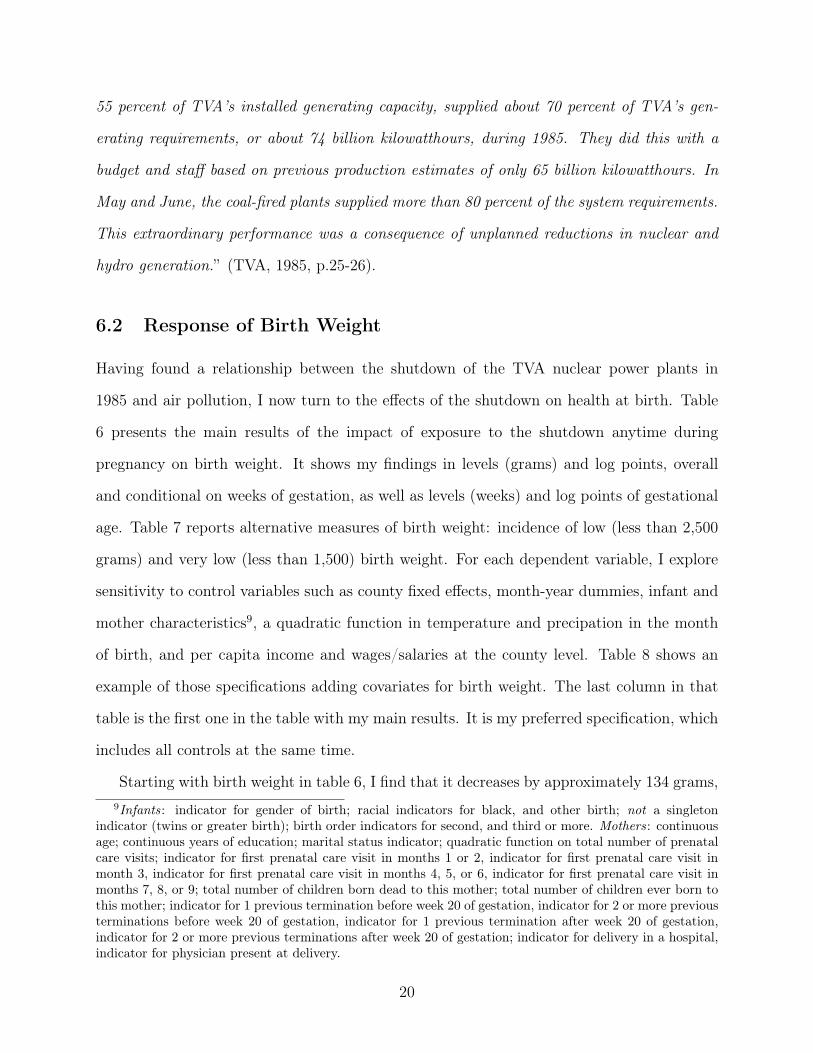
6.2 Response of Birth Weight

Having found a relationship between the shutdown of the TVA nuclear power plants in

1985 and air pollution, I now turn to the effects of the shutdown on health at birth. Table

6 presents the main results of the impact of exposure to the shutdown anytime during

pregnancy on birth weight. It shows my findings in levels (grams) and log points, overall

and conditional on weeks of gestation, as well as levels (weeks) and log points of gestational

age. Table 7 reports alternative measures of birth weight: incidence of low (less than 2,500

grams) and very low (less than 1,500) birth weight. For each dependent variable, I explore

sensitivity to control variables such as county fixed effects, month-year dummies, infant and

mother characteristics9, a quadratic function in temperature and precipation in the month

of birth, and per capita income and wages/salaries at the county level. Table 8 shows an

example of those specifications adding covariates for birth weight. The last column in that

table is the first one in the table with my main results. It is my preferred specification, which

includes all controls at the same time.

Starting with birth weight in table 6, I find that it decreases by approximately 134 grams,9Infants: indicator for gender of birth; racial indicators for black, and other birth; not a singleton

indicator (twins or greater birth); birth order indicators for second, and third or more. Mothers: continuousage; continuous years of education; marital status indicator; quadratic function on total number of prenatalcare visits; indicator for first prenatal care visit in months 1 or 2, indicator for first prenatal care visit inmonth 3, indicator for first prenatal care visit in months 4, 5, or 6, indicator for first prenatal care visit inmonths 7, 8, or 9; total number of children born dead to this mother; total number of children ever born tothis mother; indicator for 1 previous termination before week 20 of gestation, indicator for 2 or more previousterminations before week 20 of gestation, indicator for 1 previous termination after week 20 of gestation,indicator for 2 or more previous terminations after week 20 of gestation; indicator for delivery in a hospital,indicator for physician present at delivery.

20

or 5.4 log points, after the nuclear shutdown. Keep in mind that the mean birth weight before

the shutdown is roughly 3,267 grams. Notice, though, that the effect emerges only when coal

power generation responds strongly to the shutdown, and TSP concentration jumps from the

40s to the 50s µg/m3. In fact, the test of equality of the coefficients from the high response

and the medium response in terms of power generation indicates that those estimates are

statistically different at conventional levels. If we assume that the only pollutant affected

by coal power generation in response to the shutdown is TSP, we can compute the impact

of TSP on birth weight by dividing the effect of the shutdown on birth weight by the effect

of the shutdown on TSP, as shown in table 4, akin to instrumental variables (IV). This

procedure suggests that exposure to an additional 1 µg/m3 of TSP during pregnancy after

the shutdown decreases birth weight by approximately 11 grams. As discussed by Lavaine

and Neidell (2013) in a similar context, one should be cautious in interpreting this last

finding. Coal-fired power plants may have affected other pollutants in their response to the

nuclear shutdown, and this would violate the exclusion restriction of a valid IV. Indeed, as

mentioned before and shown in table 4, the shutdown might have increased SO2 levels as

well, even though such increase seems to be uncorrelated with responses from coal plants.

It is imperative to mention that my estimates are at least twice as larger as those effects

found in epidemiological studies. In a systematic review and meta-analysis of the impact

of ambient air pollution on birth weight, Stieb et al. (2012) find that an increase of 10

µg/m3 in PM10 and PM2.5 concentration reduces birth weight by 8.4 and 11.7 grams, re-

spectively. Using the EPA correspondences between measures of TSP, PM10 and PM2.510,

those effects could be translated into reductions of 17.5 and 42 grams, respectively, when

TSP concentration increases by 10 µg/m3.

One could be interested in disentangling the negative impact of the shutdown on birth

weight into two components: (i) slower fetal growth, and (ii) shorter gestation. The reduc-

tion of 134 grams has not been conditioned on gestational age, another potential variable10The TSP/PM10 ratio is 0.48 (Pace and Frank, 1986, Table 1), and the PM10/PM2.5 ratio is 0.58

(Parkhurst et al., 1999, Table 3).

21

affected by the shutdown. When I control flexibly for weeks of gestation - quartic function

in gestational age -, the effect on birth weight reduces 35 percent to roughly 87 grams, as

shown in the third column of table 6. Thus, growth retardation might explain 65 percent of

the impact of the nuclear shutdown on birth weight. Therefore, it does appear that the nu-

clear shutdown induces deleterious effects on health at birth through both channels: growth

retardation and shorter gestation11. Moreover, both effects seem to have economic signifi-

cance. Taken together, these results differ from those of the impact of a recent strike in oil

refineries in France, studied by Lavaine and Neidell (2013). They suggest that the increase

in birth weight, driven likely by a decrease in SO2 concentration, might be solely due to

shorter gestation, rather than growth retardation.

Nevertheless, the role of prematurity is still non-negligible. Indeed, looking directly at

gestational age, my estimates from columns 5 and 6 of table 6 indicate that the shutdown

decreases weeks of gestation by roughly 0.54 weeks, or 3.8 days, or 1.5 log points. Here,

though, the p-value of the test of equality of the coefficients from the high response and

the medium response in terms of power generation is much higher. Keep in mind that the

baseline mean is approximately 39 weeks. This yields an "IV" estimate of a reduction of

0.32 days of gestational length for each 1 µg/m3 increase in TSP concentration driven by the

shutdown. I follow Lavaine and Neidell (2013) to translate this effect in weeks into weight.

Fetuses gain about 200 grams per week in the final month of pregnancy (Cunningham et al.,

2010). Hence, the 0.54 week decrease in gestation translates into a reduction of 108 grams in

weight. Given that the coefficients from the high response and the medium response in terms

of power generation are statistically similar, though, one cannot rule out that the effect is as

small as 60 grams, which is very close to the amount explained by shorter gestation in the

birth weight regressions.11Air pollution is hypothesized to affect the fetus directly through transplacental exposure or indirectly by

adversely impacting maternal health during pregnancy. Although the mechanisms of toxicity of air pollutionon the fetus are poorly understood, several have been proposed, particularly for PM effects, includingoxidative stress, pulmonary and placental inflammation, blood coagulation, endothelial dysfunction andchanges in diastolic and systolic blood pressure (Kannan et al., 2006).

22

Turning to the incidence of low birth weight - less than 2,500 grams -, my estimates from

the first column of table 7 suggest that it increases by approximately 2 percent after the

nuclear shutdown in the county where coal-fired power generation responded strongly to the

shutdown. An impact of opposite sign but similar magnitude is found for the county that

had a medium response in terms of power generation. Those effects are even stronger for

the incidence of very low birth weight - less than 1,500 grams, as shown in the column 4.

Keep in mind that low birth weight is a rare event in the TVA area. Indeed, even before

the shutdown, the tenth percentile of birth weight was already above that threshold: 2,580

grams. Again, I control flexibly for weeks of gestation to check if these findings can be

explained by shorter gestation. Estimates from column 2 indicate that prematurity may

play a major role in this context, although not enough to explain the whole pattern. Thus, I

consider the possibility that my estimates may also reflect the fact that the response to the

shutdown may have improved the economic status of households by bringing more economic

activity to locations with coal-powered plants. Even though I control for changes in per

capita income and per capita wages/salaries at the county level, those variables might not

capture well changes in earnings at the household level. In such a case, my estimates would

reflect only the net effect of additional pollution and earnings. Hence, in the third column of

table 7 I control directly by changes in the number of jobs and wage bills in those coal-fired

power plants brought about by the response to the nuclear shutdown. It appears that such

variables explain the overall pattern of the effects on the probability of low birth weight12. In

fact, both coefficients are much smaller and no longer statistically significant. Furthermore,

the test of equality of the coefficients from the high response and the medium response in

terms of power generation indicates that those estimates are statistically identical to zero.

A similar pattern is found for very low birth weight in columns 5 and 6.

It is important to say that all these results survive a number of robustness checks. First,

they are robust to the time frame used in the estimation, as we can see in table 9, where12As we will see in the next paragraph, this is not the case for my main birth weight results.

23

I present estimates for one to two year windows. Also, as shown in table 10, they are

not very sensitive to (i) including changes in the number of jobs and wage bills in coal-

fired power plants associated with the response to the nuclear shutdown, (ii) adding climate

variables - average temperature and total precipitation - for each trimester during pregnancy

(Currie and Schwandt, 2013), (iii) incorporating infants from two neighboring counties which

both contain coal-powered plants (Kingston and Bull Run Coal Plants), which could share

pollution and economic activity driven by the response to the shutdown (iv) excluding babies

from the county where Allen Fossil Plant is located, which is in the control group but has the

majority of observations in my sample, and because the plant was built in the 1950s by the

Memphis Light, Gas, and Water Division, leased to TVA in 1965, and purchased outright

by TVA in 1984, (v) weighting a few observations from states that reported only half of the

births, and (vi) reweighting by the number of births in each county due to differences in

sample sizes across counties.

In their review and meta-analysis, Stieb et al. (2012) find an enormous variation in the

effects of air pollution by exposure period and recommend further exploration. Here, given

that women are in different stages of pregnancy by the time of the shutdown, it is possible

to determine whether the impact on health outcomes at birth depends on the length of the

exposure to TSP. To exploit this source of variation, I interact the dummy of the nuclear

shutdown with each trimester the baby was born before and after the shutdown. If the infant

is born in the first quarter following the shutdown, for instance, that means that exposure

to additional air pollution in utero was at most three months. Table 11 presents my results

controlling for the same covariates mentioned previously for my preferred specification, and

figure 7 present the event study graph.

Although babies born in the first trimester after the shutdown do not appear to be

negatively affected, I find that most of the impact of the shutdown on birth weight comes

from infants that are exposed to additional TSP for at least six months. Furthermore,

the effects seem to be increasing in exposure to additional pollution. Indeed, the effect is

24

97 grams for infants born in the second trimester following the shutdown, 146 grams for

babies born in the third trimester, and of similar magnitude thereafter. Beacuse there is no

evidence of a decline in the impact on birth weight after three trimesters, migration responses

to higher TSP concentration might be negligible. Nine months would be more than enough

for households to find a location with lower levels of pollution. Again, the impact is found

only for the group experiencing the highest coal power generation response. If anything, the

effect for the medium response group would be positive, but the coefficients are generally

statistically zero.

Figure 7 actually motivates the regression analysis for birth weight discussed previously.

It plots coefficients for each group of response to the nuclear shutdown and their 95 percent

confidence intervals. They provide an opportunity to judge the validity of the difference-

in-differences-style approach that is based on the assumption of similar trends in advance

of the shutdown. That figure does seem to support the validity of the design as there is

little evidence of differential trends in birth weight for each of the treatment groups in the

trimesters preceding the shutdown.

Because of strong seasonal patterns of pollution and other environmental confounders,

I evaluate the validity of my research design by running a falsification test. Basically, I

assign the date of the nuclear shutdown to have occured in March 1979, a few years before

the actual one13. A severe recession happens in the early 1980s - July 1981 to November

1982 -, generating substantial variation in air pollution across sites, as exploited by Chay

and Greenstone (2003) to study the impact of air pollution on infant mortality. If I had

assigned the placebo shutdown to happen in March 1983, two years before the actual nuclear

shutdown, the pre-placebo shutdown would have included a substantial period of the 1981-

1982 recession. I end up using March 1979 instead. It still includes a recession from the

early 1980s, but it is a much shorter one - January to July 1980. As shown in tables 12, 1313Recall that my time frame for the estimation is eighteen months before and after the shutdown. This is

the reason why I do not assign the placebo shutdown to have happened in the year immediately before theactual one.

25

and 13, I find that the placebo shutdown is broadly neither associated with TSP levels14 nor

measures of health at birth.

6.3 "Safe" Threshold for Exposure to TSP

Having found plenty of evidence that high levels of pollution are harmful, Currie et al. (2014)

suggest that a "particularly important question for policy is whether there is a safe level of

these substances." (p.20) for fetuses and young children. In other words, they urge recovering

a curve of pollution effects as a function of pollution exposure. My attempt to infer such

a dose response function in the context of my study is quite primitive, but might still shed

some light on the safe threshold for TSP, and may inspire further research.

I begin by noticing that TSP concentrations displayed in the right-hand side of table 1

do not appear to respond proportionally to the coal power generation driven by the nuclear

shutdown. Although the medium group generates only two thirds of the additional electricity

produced by the high group, TSP responses seem to be very similar. Indeed, when I plot

the smoothed data on TSP concentration in figure 3, the only difference in the observed

patterns seems to be the level of pollution that each group starts with. The medium group

jumps from the 30s to the 40s µg/m3, whereas the high group moves from the 40s to the

50s µg/m3. Just for reference, the EPA annual standard for TSP is 75 µg/m3 from 1971 to

1987.

Proceeding with my difference-in-differences estimation approach, I find that, in 1985,

even though TSP concentrations are below EPA standards, they are not at safe levels. When

TSP concentration is above 50 µg/m3, but still below the standard of 75 µg/m3, air pollution

seems to decrease birth weight by roughly 3.7 percent, and gestational age by 0.67 weeks,

as discussed previously. However, no statistically significant effects are found for TSP levels14Although some TSP effects seem to be statistically significant in a couple of counties after the placebo

shutdown, notice that those effects are significant only where responses from coal-powered plants are notsignificant. The apparent spatially heterogeneous decrease in TSP might be related to emission reductionsfrom other sectors, which may be facing a short recession in the post-placebo nuclear shutdown. In fact, ifanything, coal-fired power generation may have increased in those counties where the negative TSP effectsare statistically significant.

26

below 50 µg/m3. From this comparison, I primitively infer that 50 µg/m3 might be a safe

threshold for exposure to TSP. I say "primitive" because I am not testing for any break

around 50 µg/m3. Furthermore, the difference of the coefficients from the high response and

the medium response in terms of power generation is somewhat imprecisely estimated, even

though the p-values are much lower than those found in the placebo tests.

In 1987, EPA replaces the earlier TSP air quality standard with a PM10 standard. A

decade later, a PM2.5 standard is added. The new standards focus on smaller particles that

are likely responsible for adverse health effects because of their ability to reach the lower

regions of the respiratory tract. I use EPA correspondences between measures of those three

elements15 to translate TSP to PM levels, and to evaluate the standards vis-à-vis the inferred

threshold. My findings suggest that EPA might have set the TSP and PM standards right

only from 1997 onwards, as shown in table 2. This illustrates that the research design used

in this study might help EPA setting the NAAQS for other pollutants.

7 Concluding Remarks

When environmental regulations focus on a subset of power plants, the ultimate goal of

human health protection may not be reached. Because power plants are interconnected

through the electrical grid, excessive scrutiny of a group of facilities may generate more pol-

lution out of another group, with potential deleterious effects to public health. In this study,

I investigate the impact of the shutdown of nuclear power plants in the Tennessee Valley

Authority (TVA), in 1985, on health outcomes at birth. After the Three Mile Island acci-

dent in 1979, the Nuclear Regulatory Commission (NRC) intensified inspections in nuclear

facilities leading to shutdown of many of them, including Browns Ferry and Sequoyah in the

TVA area.

I have four main findings. I first show that, in response to the shutdown, electricity15The TSP/PM10 ratio is 0.48 (Pace and Frank, 1986, Table 1), and the PM10/PM2.5 ratio is 0.58

(Parkhurst et al., 1999, Table 3).

27

generation shifted mostly to coal-fired power plants within the TVA, increasing air pollution

in counties where they were located. I provide evidence that the substitution of coal for

nuclear power generation may be one to one. Also, that TSP concentration, my measure

of pollution, responds only in counties hosting the coal-powered plants with the highest

increases in coal-burning generation due to the shutdown.

Second, I find that babies born after the nuclear shutdown have both lower birth weight

and lower gestational age in those counties with coal-fired power plants that do respond to the

shutdown. This indicates that exposure to higher levels of TSP may deteriorate infant health

via two channels: growth retardation and shorter gestation. Third, I highlight the presence

of substantial heterogeneity in those effects depending on how much more electricity those

coal-powered facilities were generating in response to the shutdown. For the group with

the highest response in terms of both coal-burning generation and TSP concentration, it

seems that exposure to an additional 1 µg/m3 of TSP during pregnancy after the shutdown

induces a reduction of roughly 11 grams in birth weight. Furthermore, both fetal growth and

gestational length appear to be affected negatively by the shutdown. I find no statistically

significant effects when coal generation responses to the shutdown are medium or low.

Summing the growth retardation and the shorter gestation effects, I estimate that birth

weight reduces by approximately 134 grams, or 5.4 percent, in those counties with coal-fired

power plants responding strongly to the nuclear shutdown. This effect is at least twice as

larger as those found by Stieb et al. (2012) in their systematic review and meta-analysis of

the impact of ambient air pollution on birth weight. To get a sense of the magnitude of my

estimate, I consider the U.S. Special Supplemental Nutrition Program for Women, Infants,

and Children (WIC) program, which among other things provides supplemental foods, health

care referrals, and nutrition education for low-income pregnant women. Kowaleski-Jones and

Duncan (2002) estimate that participation in the WIC by a pregnant woman increases child

birth weight by 7.5 percent, which is almost the opposite effect induced by the nuclear

shutdown. Using the impact of birth weight on adult outcomes from Black, Devereux and

28

Salvanes (2007), a 5.4 percent reduction in birth weight would lead to a 0.7 percent decrease

in full-time earnings, a 0.4 centimeter decrease in height, a 0.04 stanine decrease in IQ, and

a 0.8 percent decrease in the birth weight of their children16. Isen, Rossin-Slater and Walker

(2015) calculate that the mean present value of lifetime earnings at age zero in the U.S.

population is $434,000 (2008 dollars) using a real discount rate of 3 percent (i.e., a 5 percent

discount rate with 2 percent wage growth). Thus, the financial value of being born into a

county with a coal-fired power plant responding to the nuclear shutdown in the months after

the shutdown is 0.7 percent of $434,000 or $3,038 per person.

Lastly, I use the heterogeneity in response to the nuclear shutdown to provide suggestive

evidence on the "safe" threshold of exposure to TSP, which can potentially guide the Envi-

ronmental Protection Agency (EPA) in setting the National Ambient Air Quality Standards

(NAAQS) for particulate matters. Although I find no significant impact on health at birth

associated with medium coal generation response to the shutdown, TSP levels do increase

in those locations. The crucial difference among counties with high and medium responses

is the level of TSP that they start with. In the high response group, it jumps from the 40s

to the 50s µg/m3, whereas in the medium response group it moves from the 30s to the 40s

µg/m3. Hence, the "safe" threshold for exposure to TSP might be 50 µg/m3, which is close

to the current EPA standards for PM when translated to the PM10 and PM2.5 scales.

Taking together, these findings make four contributions to the literature and policymak-

ing. First, they point out that environmental regulations focused on one node of an extensive

network of energy production may trigger unanticipated chain reactions that go against the

ultimate goal of protecting public health. Networks should be taken into account in the

design of those regulations. Second, they show that a curve relating effects of pollution on

health and intensity of pollution exposure may be estimable through the use of networks.

When shocks in one node produce different responses over other nodes, quasi-experimental16Black, Devereux and Salvanes (2007) estimate that each 1 percent decrease in birth weight decreases

expected earnings by 0.13 percent, height by 0.07 centimeter, IQ stanine by 0.007, and birth weight of theirchildren by 0.15 percent.

29

variation in pollution exposure may arise. As already discussed, this methodology has the

potential to guide EPA when setting the NAAQS. Third, they provide evidence that sus-

pending nuclear energy production might not generate as many net benefits as the public

perceives. The retirement of the San Onofre Nuclear Generating Station in California, and

the denuclearization Germany intensified after the Fukushima disaster, may actually bring

about unintended net costs to society. Lastly, they corroborate recent findings by Lavaine

and Neidell (2013) that pollution externalities from energy production are also prominent,

and should be seriously considered in the design of environmental policies.

References

- Almond, Douglas, Kenneth Y. Chay, and David S. Lee. (2005). The Costs of Low Birth

Weight, Quarterly Journal of Economics 120(3): 1031-1083.

- Almond, Douglas, Lena Edlund and Mårten Palme. (2009). Chernobyl’s Subclinical

Legacy: Prenatal Exposure to Radioactive Fallout and School Outcomes in Sweden, Quar-

terly Journal of Economics 124 (4): 1729-1772.

- Black, Sandra E., Paul J. Devereux, and Kjell G. Salvanes. (2007). From the Cradle

to the Labor Market? The Effect of Birth Weight on Adult Outcomes, Quarterly Journal of

Economics 122(1): 409-439.

- Black, Sandra E., Aline Bütikofer, Paul J. Devereux, and Kjell G. Salvanes. (2014).

This Is Only a Test? Long-Run and Intergenerational Impacts of Prenatal Exposure to

Radioactive Fallout, Working Paper - University of Texas at Austin.

- Cullen, Joseph. (2013). Measuring the Environmental Benefits of Wind-Generated

Electricity, American Economic Journal: Economic Policy 5(4): 107-133.

- Cunningham FG, Leveno KJ, Bloom SL, et al. (2010). "Fetal growth and development."

In: Cunnigham FG, Leveno KL, Bloom SL, Hauth, JC, Rouse DJ, Spong CY, eds. Williams

Obstetrics. 23rd ed. New York, NY: McGraw-Hill; chap 4.

30

- Currie, Janet, and Hannes Schwandt. (2013). Within-Mother Analysis of Seasonal

Patterns in Health at Birth, Proceedings of the National Academy of Sciences 110(30): 12265-

12270.

- Currie, Janet, Joshua S. Graff Zivin, Jamie Mullins, and Matthew J. Neidell. (2014).

What Do We Know About Short and Long Term Effects of Early Life Exposure to Pollution?,

Annual Review of Resource Economics 6: 217-247.

- Goebel, Jan, Christian Krekel, Tim Tiefenbach, and Nicolas R. Ziebarth. (2013).

Natural Disaster, Policy Action, and Mental Well-Being: The Case of Fukushima, IZA DP

No. 7691.

- Isen, Adam, Maya Rossin-Slater, and W. Reed Walker. (2015). Every Breath You Take

- Every Dollar You’ll Make: The Long-Term Consequences of the Clean Air Act of 1970,

Working Paper, University of California, Berkeley.

- Kannan S., D. Misra, J. Dvonch, and A. Krisnakamar. (2006). Exposures to Airborne

Particulate Matter and Adverse Perinatal Outcomes: A Biologically Plausible Mechanistic

Framework for Exploring Potential Effect Modification by Nutrition, Environmental Health

Perspectives 114(11):1636-1642.

- Kowaleski-Jones, Lori, and Greg J. Duncan. (2002). Effects of Participation in the

WIC Program on Birthweight: Evidence From the National Longitudinal Survey of Youth,

American Journal of Public Health 92(5): 799-804.

- Lavaine, Emmanuelle, and Matthew J. Neidell. (2013). Energy Production and Health

Externalities: Evidence From Oil Refinery Strikes in France, NBER Working Paper 18974.

- Lewis, Joshua, and Edson R. Severnini. (2014). The Value of Rural Electricity: Evi-

dence from the Rollout of the U.S. Power Grid, Working Paper - Carnegie Mellon University.

- Pace, Thompson G., and Neil H. Frank. (1986). Procedures for Estimating Probability

of Nonattainment of a PM10 NAAQS Using Total Suspended Particulate or PM10 data, U.S.

Environmental Protection Agency Report EPA-450/4-86-017.

- Parkhurst, William J., Roger L. Tanner, Frances P. Weatherford, Ralph J. Valente,

31

and James F. Meagher. (1999). Historic PM10/PM2.5 Concentrations in the Southeastern

United States - Potential Implications of the Revised Particulate Matter Standard, Journal

of the Air & Waste Management Association 49(9): 1060-1067.

- Stieb, David M., Li Chen, Maysoon Eshoul, and Stan Judek. (2012). Ambient air

pollution, birth weight and preterm birth: A Systematic Review and Meta-Analysis, Envi-

ronmental Research 117: 100-111.

- Tennessee Valley Authority (TVA). (1985). 1985 Annual Report. Available at hathitrust.org.

- Tennessee Valley Authority (TVA). (1986). 1986 Annual Report. Available at hathitrust.org.

32

Appendix A

The shutdown of the TVA nuclear power plants in 1985 triggered a response in terms of power

generation by TVA coal-fired power plants. County fixed-effect regressions using annual data

for all coal plants from 1982 until 1987 reveal that most of that response vanishes away when

one controls for technology and cost variables. That is, the cost structure of coal plants can

explain relatively well the observed power generation response, suggesting that society’s

pressure to avoid exposure to pollution might not have been the underlying force behind the

heterogeneity in response across plants.

Tables A.1 and A.2 show the results. In the first column, only the dummy for the nuclear

shutdown is included, and its coefficient is statistically significant. In the second column,

efficiency - a proxy for plant technology - is added, and its coefficient is also significant, but

it does not change the magnitude and significance of the effect of the nuclear shutdown.

The third column incorporates the cost per kW of installed capacity, reflecting the sunk

investment in those power plants. Its coefficient does not seem to be an important factor

affecting the response to the nuclear shutdown. The fourth column adds the cost of coal by

cents per million Btu, and its coefficient is significant and does affect the association between

the nuclear shutdown and the dependent variables. Lastly, in the fifth column, the Clean

Air Act non-attainment designation is included, without any impact on the coefficient of the

other covariates. Therefore, it appears that variable costs in coal-fired power plants may be

the driving force of the power generation response to the nuclear shutdown.

Table A.3 presents the summary statistics of all variables mentioned above. As we can

see, the plant with the highest power generation response - Paradise - had the lowest coal

costs before the nuclear shutdown. Similarly, Cumberland, the plant with the second high-

est response, had the largest reduction in coal costs after the shutdown. These pieces of

information illustrate the underlying importance of cost considerations in the reaction to the

shutdown. Indeed, the overall reduction in coal costs is the most noticeable feature of table

A.3.

33

It is also interesting to see that the response to the nuclear shutdown did not happen

through the Allen power plant, which is close to one of the largest urban centers in the TVA

area, but did affect power generation at Paradise, situated in a county with small population

density. Since both plants were in counties out of attainment under the Clean Air Act, it

might be the case that TVA was trying to act like a social planner, although regression

analysis did not corroborate this line of reasoning, and air pollution was never a front and

center issue in TVA annual reports.

Table A.1: Reasons for the Power Generation Response

Table A.2: Reasons for the Capacity Factor Response

34

Table A.3: Reasons for Response - Summary Statistics

35

Figure 1: TVA Power Generation (Terawatt Hours)

02

46

8

1983m9

1984m3

1984m9

1985m3

1985m9

1986m3

1986m9

Coal Nuclear Hydro

Notes: This figure plots monthly EIA electricity generation data at the plant-fuel level in the TVA area. Kernel-weighted localpolynomial regressions of those monthly values on time provide the smoothed values graphed in the figure. (The kernel functionused in the smoothing was Epanechnikov, the kernel bandwidth was six, and the degree of the polynomial smooth was zero.)The first solid vertical is at March 1985, when the first TVA nuclear power plant - Browns Ferry - was shut down. The secondsolid vertical is at August 1985, when the second and last TVA nuclear power plant - Sequoyah - was shut down.

36

Figure 2: TSP Concentration - >50 µg/m3 vs. <50 µg/m3

202530354045505560657075

1983m91984m3

1984m91985m3

1985m91986m3

1986m9

H-∆PG M-∆PG 1971-87 Annual Standard: 75µg/m3

Notes: This figure plots monthly TSP data from EPA at the county level in the TVA area. Kernel-weighted local polynomialregressions of those monthly values on time provide the smoothed values graphed in the figure. (The kernel function used in thesmoothing was Epanechnikov, the kernel bandwidth was six, and the degree of the polynomial smooth was zero.) The first solidvertical is at March 1985, when the first TVA nuclear power plant - Browns Ferry - was shut down. The second solid verticalis at August 1985, when the second and last TVA nuclear power plant - Sequoyah - was shut down. H ��PG represents thecounty with a coal-fired power plant with a high response to the nuclear shutdown in terms of power generation. M � �PGrepresents the county with a coal plant with a medium response to the nuclear shutdown. The "Annual Standard" refers to theNational Ambient Air Quality Standards (NAAQS) for TSP set by EPA in 1971.

37

Figure 3: Birth Weight - >50 µg/m3 vs. <50 µg/m3

3100

3200

3300

3400

3500

3600

3700

1983m9

1984m3

1984m9

1985m3

1985m9

1986m3

1986m9

H-∆PG M-∆PG

Notes: This figure plots birth weight data from the National Vital Statistics System at the county level in the TVA area. Eachdot represents the average birth weight of all babies born in a month in a county in the TVA area. Only values between 3,100and 3,700 grams are shown in the scatterplot to make it easier to see the changes in (smoothed) birth weight. Kernel-weightedlocal polynomial regressions of those monthly values on time provide the smoothed values graphed in the figure. (The kernelfunction used in the smoothing was Epanechnikov, the kernel bandwidth was nine, and the degree of the polynomial smoothwas zero.) The first solid vertical is at March 1985, when the first TVA nuclear power plant - Browns Ferry - was shut down.The second solid vertical is at August 1985, when the second and last TVA nuclear power plant - Sequoyah - was shut down.H ��PG represents the county with a coal-fired power plant with a high response to the nuclear shutdown in terms of powergeneration. M ��PG represents the county with a coal plant with a medium response to the nuclear shutdown.

38

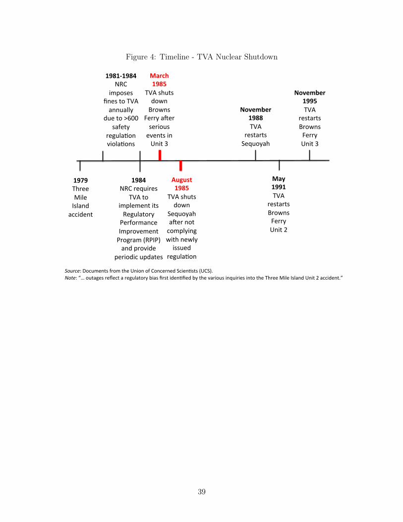
Figure 4: Timeline - TVA Nuclear Shutdown

1979!Three!Mile!Island!

accident!

1981%1984NRC!

imposes!fines!to!TVA!annually!

due!to!>600!safety!

regula@on!viola@ons!

1984!!!!!!!!!!!!!!!NRC!requires!

TVA!to!implement!its!Regulatory!Performance!Improvement!Program!(RPIP)!and!provide!

periodic!updates!

March,1985!!!!!

TVA!shuts!down!Browns!

Ferry!aIer!serious!events!in!Unit!3!!

August,1985!!!!!

TVA!shuts!down!

Sequoyah!aIer!not!complying!with!newly!issued!

regula@on!

November,1988!!!!!TVA!

restarts!Sequoyah!

May,1991!!!!!TVA!

restarts!Browns!Ferry!Unit!2!

November,1995!!!!!TVA!

restarts!Browns!Ferry!!!!!Unit!3!

Source:!Documents!from!the!Union!of!Concerned!Scien@sts!(UCS).!!!Note:!“…!outages!reflect!a!regulatory!bias!first!iden@fied!by!the!various!inquiries!into!the!Three!Mile!Island!Unit!2!accident.”!

39

Figure 5: Map of TVA Power Plants - 1985

Figure 6: Map of TVA Coal and Nuclear Power Plants -1985

40

Figure 7: Birth Weight - Event Study of the Nuclear Shutdown

-200

020

0Bi

rth W

eigh

t - G

ram

s

-5 -4 -3 -2 -1 0 1 2 3 4 5Trimester Relative to Nuclear Shutdown

H-∆PG M-∆PG L-∆PG

Notes: This figure plots the coefficients of an event study regression based on equation 11 for birth weight. The analysis spansfive trimesters before and after the TVA nuclear shutdown in March 1985.

41

Table 1: Heterogeneity in response to nuclear shutdown

Notes: This table presents some summary statistics for TVA counties classified in one of the groups based on intensity of theresponse to the nuclear shutdown: H � �PG (high response), M � �PG (medium response), L � �PG (low response), andN � �PG (negligible response). "PG" represents power generation, "TSP" total suspended particles, and "BWeight" birthweight.

Table 2: EPA Standards and "Safe" Threshold - TSP, PM10 and PM2.5

Annual TSP PM10 PM2.5Standards1971-87 75µg/m3

1987-97 50µg/m3

1997-06 50µg/m3 15µg/m3

2006-12 15µg/m3

2012-... 12µg/m3

Suggestive50µg/m3 24µg/m3 14µg/m3

ThresholdSource: epa.gov/ttn/naaqs/standards/pm/s_pm_history.html

42

Table 3: Sample for Birth Weight Analysis

Notes: This table presents some summary statistics for TVA counties classified in one of the groups based on intensity of theresponse to the nuclear shutdown: H � �PG (high response), M � �PG (medium response), L � �PG (low response), andN��PG (negligible response). Each row shows the name of the coal-fired plant located in the county whose data are tabulatedabove. "Main" represents the sample used in the main analysis, and it refers to the first two columns of data in the table. Thelast two columns include information on two counties which have coal plants but are neighbors. They are excluded from themain analysis because of potential pollution spillovers. (Results are robust to their inclusion.)

43

Table 4: Response of Power Generation and Pollution - Coal

44

Table 5: Response of Power Generation and Pollution - Hydro

45

Table 6: Response of Birth Weight - Main Results and Mechanisms

Notes: Standard errors clustered by county and month/year in parentheses. *** Significant at the 1 percent level. ** Significantat the 5 percent level. * Significant at the 10 percent level. Control variables from my preferred specification are county fixedeffects, month-year dummies, infant and mother characteristics, a quadratic function in temperature and precipation in themonth of birth, and per capita income and wages/salaries at the county level.

Table 7: Response of Birth Weight - Low Birth Weight

Notes: Standard errors clustered by county and month/year in parentheses. *** Significant at the 1 percent level. ** Significantat the 5 percent level. * Significant at the 10 percent level. Control variables from my preferred specification are county fixedeffects, month-year dummies, infant and mother characteristics, a quadratic function in temperature and precipation in themonth of birth, and per capita income and wages/salaries at the county level.

46

Table 8: Response of Birth Weight - Preferred Specification

Notes: Standard errors clustered by county and month/year in parentheses. *** Significant at the 1 percent level. ** Significantat the 5 percent level. * Significant at the 10 percent level. Control variables from my preferred specification are county fixedeffects, month-year dummies, infant and mother characteristics, a quadratic function in temperature and precipation in themonth of birth, and per capita income and wages/salaries at the county level.

Table 9: Response of Birth Weight - Robustness Checks in Time Frame

Notes: Standard errors clustered by county and month/year in parentheses. *** Significant at the 1 percent level. ** Significantat the 5 percent level. * Significant at the 10 percent level. Control variables from my preferred specification are county fixedeffects, month-year dummies, infant and mother characteristics, a quadratic function in temperature and precipation in themonth of birth, and per capita income and wages/salaries at the county level.

47

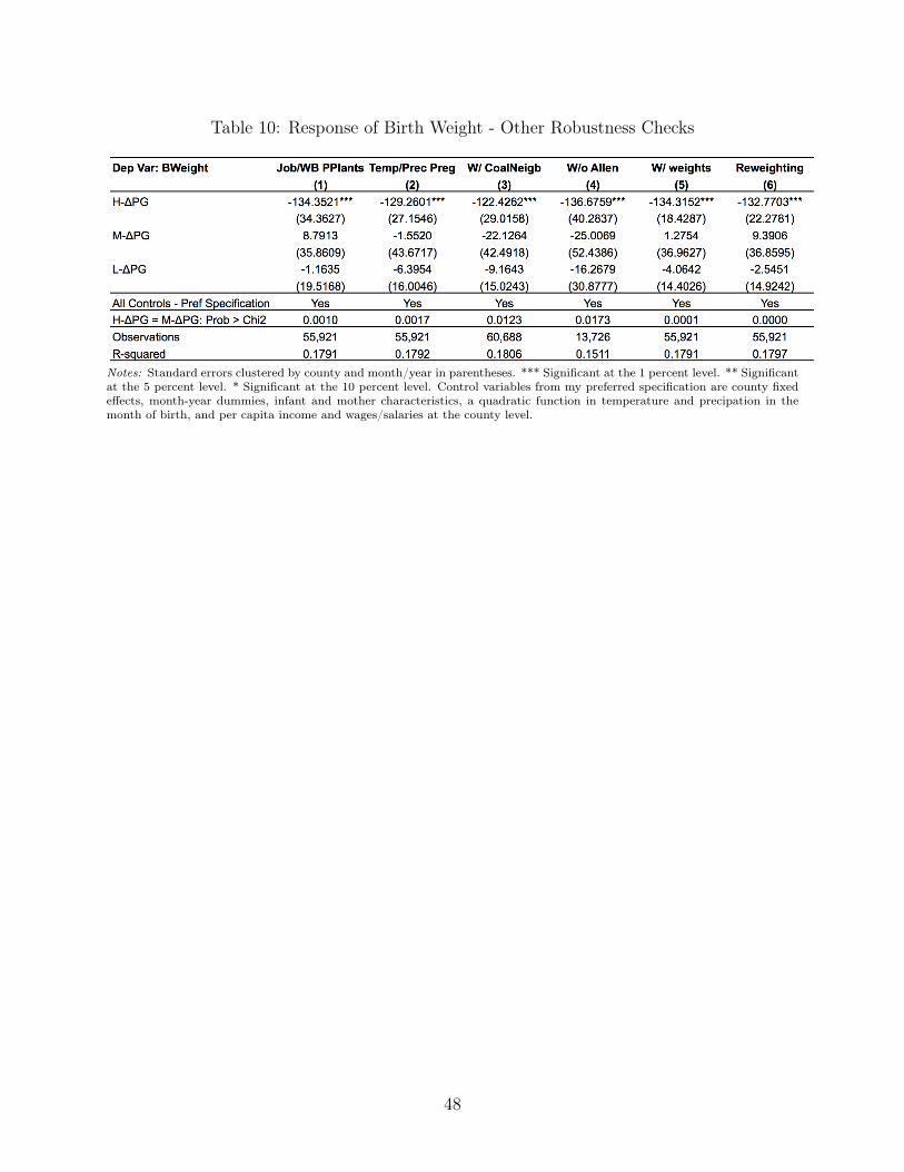
Table 10: Response of Birth Weight - Other Robustness Checks

Notes: Standard errors clustered by county and month/year in parentheses. *** Significant at the 1 percent level. ** Significantat the 5 percent level. * Significant at the 10 percent level. Control variables from my preferred specification are county fixedeffects, month-year dummies, infant and mother characteristics, a quadratic function in temperature and precipation in themonth of birth, and per capita income and wages/salaries at the county level.

48

Table 11: Response of Birth Weight - Event Study

Notes: Standard errors clustered by county and month/year in parentheses. *** Significant at the 1 percent level. ** Significantat the 5 percent level. * Significant at the 10 percent level. Control variables from my preferred specification are county fixedeffects, month-year dummies, infant and mother characteristics, a quadratic function in temperature and precipation in themonth of birth, and per capita income and wages/salaries at the county level.

49

Table 12: Response of Power Generation and Pollution - Coal - Placebo

Table 13: Response of Birth Weight and Weeks of Gestation - Placebo

Notes: Standard errors clustered by county and month/year in parentheses. *** Significant at the 1 percent level. ** Significantat the 5 percent level. * Significant at the 10 percent level. Control variables from my preferred specification are county fixedeffects, month-year dummies, infant and mother characteristics, a quadratic function in temperature and precipation in themonth of birth, and per capita income and wages/salaries at the county level.

50