nucleosynthesis in extremely metal-poor and zero ... · zusammenfassung die wachsende zahl an...
TRANSCRIPT
Nucleosynthesis in extremely
metal-poor and zero
metallicity stars
Monique Alves Cruz


Nucleosynthesis in extremely
metal-poor
and zero metallicity stars
Monique Alves Cruz
Dissertation der Fakultat fur PhysikDissertation of the Faculty of Physics
der Ludwig-Maximilians-Universitat Munchenat the Ludwig Maximilian University of Munich
fur den Grad desfor the degree of
Doctor rerum naturalium
vorgelegt von Monique Alves Cruzpresented by
aus Itamaraju, Brasilien (Brazil)from
Munich, 2012


1st Evaluator: Prof. Dr. Achim Weiss
2nd Evaluator: Prof. Dr. Joseph Mohr
Date of the oral exam: 20.12.2012

Zusammenfassung
Die wachsende Zahl an Beobachtungen metallarmer Sterne (engl. “metal-poor”, MP) hateine Vielzahl von Fragen zur Elemententstehung in der Fruhzeit unserer Galaxie aufgeworfen.In dieser Arbeit untersuchen wir die Entwicklung und die Nukleosynthese von extrem me-tallarmen und metallfreien Sternen. Fur die Metallhaufigkeit von Interesse in dieser Arbeit(0 ≤ Z ≤ 10−5) gibt es drei große Modelsatze in der Literatur (Campbell 2007; Lau et al. 2009;Suda & Fujimoto 2010). Trotzdem gibt nur eine Quelle Haufigkeiten fur Elemente schwererals Sauerstoff an. Unsere Modelle untersuchen nicht nur die leichten Elemente sondern auchdie Nukleosynthese schwerer Elemente wahrend der sogenannten “proton ingestion episode”(PIE) und die Unsicherheiten die sich fur die nukleosynthetischen Vorhersagen ergeben.
Wir finden, dass der s-Prozess wahrend der PIE sowohl in metallarmen als auch in Sternenmittlerer Metallhaufigkeit stattfindet. In massearmen Sternen geschieht die PIE wahrenddes Helium-Blitzes im Sternkern und hat großen Einfluß auf die s-Prozess Ausbeute fallsSaatkerne aus dem Haufigkeitsmaximum um Eisen im Stern vorhanden sind. MittelschwereSterne dagegen durchleben die PIE wahrend der TP-AGB Phase. Wir finden, dass die s-Prozess Ausbeute wahrend der PIE in diesen Sternen sehr stark abhangig von der Dauer derPIE ist. Außerdem wird der Großteil der s-Prozess Haufigkeit in demjenigen und dem darauffolgendem TP produziert, in dem die PIE stattfindet. Wir vergleichen unsere Produktionleichter Elemente mit denen aus Campbell 2007 und finden eine erhebliche Abweichung. DieUnterschiede konnen hauptsachlich auf das (nicht-) Vorhandensein von “hot bottom burning”wahrend der AGB Phase zuruckgefuhrt werden.
Obwohl unsere Vorhersagen zum Auftreten von s-Prozess Elemententstehung wahrend derPIE von massearmen Sternen qualitativ mit denen von Campbell et al. 2010 ubereinstimmen,findet in unseren Modelle sehr viel weniger s-Prozess statt. Wir vergleichen diese Vorhersagenmit den zwei metallarmsten Sternen die bisher beobachtet wurden. Dazu nehmen wir an,dass Masse zum beobachteten Stern ubertragen wurde und sich dann in dessen Sternhulleverteilt hat. Wir finden, dass massearme EMP Sterne mogliche Kandidaten fur einen Be-gleitstern von HE0107-5240 sind. Trotzdem sind unsere Vorhersagen nicht in der Lage, dieHaufigkeitsverteilung von HE1327-2326 zu erklaren, im Gegensatz zun den Ergebnissen inCampbell et al. 2010.
Schließlich nutzen wir ein erweitertes Netzwerk in GARSTEC um uns mit den anomalenHaufigkeiten von Sternhaufen zu befassen. Wir fanden, dass “overshooting” eine maßgeblicheRolle fur die endgultigen Haufigkeiten von O, Na, Mg und Al spielt. Wenn overshooting nichtin den Rechnung miteinbezogen wird, kann eine sehr viel bessere Ubereinstimmung mit denBeobachtungen erhalten werden.

viii

Abstract
The increasing number of metal-poor (MP) stars observed to date has raised numerousquestions concerning the elemental production in the early stages of our Galaxy. In this thesiswe study the evolution and nucleosynthesis of zero metallicity and extremely metal-poor stars.For the metallicity range covered in this thesis (0 ≤ Z ≤ 10−5) there are three large grids ofmodels in the literature (Campbell 2007; Lau et al. 2009; Suda & Fujimoto 2010). Never-theless, only one study presents abundances for elements heavier than oxygen. Our modelsexplore not only the light elements, but also the nucleosynthesis of heavy elements during theproton ingestion episode and the uncertainties affecting the nucleosynthesis predictions.
We have found that s-process does occur during the proton ingestion episode (PIE) inboth low- and intermediate-mass stars. In low-mass stars, the PIE happens during the coreHe-flash and has a strong impact in the production of s-process if iron-peak seeds are availablein the star. Intermediate-mass stars, on the other hand, undergo PIE during the TP-AGBphase. We have found that the s-process production during the PIE in these stars is stronglydependent on the duration of the ingestion. Moreover, the bulk of the surface s-processabundance is produced in the TP, in which PIE occurs, and in the subsequent TP. Wehave compared the yields of our light elements with those reported by Campbell 2007. Wehave found considerable discrepancies between the yields. This discrepancies can be mainlyascribed to the occurrence (or not) of hot bottom burning during the AGB.
Although our predictions qualitatively agree with those by Campbell et al. 2010 on theoccurrence of s-process production during the PIE of low-mass stars, our models produce farless s-process than theirs. We compared these predictions to the two most iron-poor starsobserved to date. We assumed that mass was tranferred to the observed star and it wasthen diluted in the stellar envelope. We have found that low-mass EMP stars are possiblecandidates as the companion of HE0107-5240. Nevertheless, our predictions are not able toexplain the abundance patterns in HE1327-2326 in contrast to Campbell et al. 2010 results.
Finally, we have also employed the new extended network in GARSTEC to address theglobular cluster anomalies issue. We have found that overshooting plays an important rolein the final yields of O, Na, Mg, and Al. If overshooting is not included in the calculations amuch better agreement with the observations can be obtained.

x
Contents
Zusammenfassung vii
Abstract ix
Contents xii
List of Figures xv
List of Tables xvii
1 Introduction 1
1.1 CEMP stars . . . . . . . . . . . . . . . . . . . . . . . . . . . . . . . . . . . . . 3
1.2 The most iron-poor stars . . . . . . . . . . . . . . . . . . . . . . . . . . . . . . 6
1.3 Primordial Stars . . . . . . . . . . . . . . . . . . . . . . . . . . . . . . . . . . 7
1.4 Outline . . . . . . . . . . . . . . . . . . . . . . . . . . . . . . . . . . . . . . . 8
2 On the Evolution of Moderate-Mass stars 11
2.1 Introduction . . . . . . . . . . . . . . . . . . . . . . . . . . . . . . . . . . . . . 12
2.2 Evolution pre-AGB phase . . . . . . . . . . . . . . . . . . . . . . . . . . . . . 12
2.2.1 Low-Mass Stars . . . . . . . . . . . . . . . . . . . . . . . . . . . . . . . 12
2.2.2 Intermediate-Mass Stars . . . . . . . . . . . . . . . . . . . . . . . . . . 14
2.3 Thermal-Pulse phase . . . . . . . . . . . . . . . . . . . . . . . . . . . . . . . . 18
2.4 Formation of Heavy Elements . . . . . . . . . . . . . . . . . . . . . . . . . . . 21
2.4.1 S-process . . . . . . . . . . . . . . . . . . . . . . . . . . . . . . . . . . 23
2.4.2 Classical Model and The S-process Components . . . . . . . . . . . . 23
2.4.3 The 13C Pocket . . . . . . . . . . . . . . . . . . . . . . . . . . . . . . . 25
2.5 Proton Ingestion Episode . . . . . . . . . . . . . . . . . . . . . . . . . . . . . 26
2.6 Summary . . . . . . . . . . . . . . . . . . . . . . . . . . . . . . . . . . . . . . 31
3 The evolutionary Code 33
3.1 Evolutionary Code: Basics . . . . . . . . . . . . . . . . . . . . . . . . . . . . . 34
3.2 Physical Input . . . . . . . . . . . . . . . . . . . . . . . . . . . . . . . . . . . 36
3.2.1 Opacity . . . . . . . . . . . . . . . . . . . . . . . . . . . . . . . . . . . 36
3.2.2 Nuclear Network . . . . . . . . . . . . . . . . . . . . . . . . . . . . . . 37

xii CONTENTS
3.2.3 Mass-Loss . . . . . . . . . . . . . . . . . . . . . . . . . . . . . . . . . . 423.3 Overshooting . . . . . . . . . . . . . . . . . . . . . . . . . . . . . . . . . . . . 44
4 SPNUC: The s-process Code 47
4.1 The network . . . . . . . . . . . . . . . . . . . . . . . . . . . . . . . . . . . . . 494.2 The number of subtimesteps . . . . . . . . . . . . . . . . . . . . . . . . . . . . 51
5 Low-Mass Stars 55
5.1 Introduction . . . . . . . . . . . . . . . . . . . . . . . . . . . . . . . . . . . . . 555.2 The Models . . . . . . . . . . . . . . . . . . . . . . . . . . . . . . . . . . . . . 565.3 From the ZAMS to the PIE . . . . . . . . . . . . . . . . . . . . . . . . . . . . 575.4 Main Characteristics of the Proton Ingestion Episode . . . . . . . . . . . . . . 595.5 Neutron Production and the s-process . . . . . . . . . . . . . . . . . . . . . . 64
5.5.1 The influence of convective mixing . . . . . . . . . . . . . . . . . . . . 685.5.2 The absence of iron-peak seeds: zero metallicity case . . . . . . . . . . 70
5.6 Lithium Production . . . . . . . . . . . . . . . . . . . . . . . . . . . . . . . . 715.7 Light elements . . . . . . . . . . . . . . . . . . . . . . . . . . . . . . . . . . . 735.8 Discussion . . . . . . . . . . . . . . . . . . . . . . . . . . . . . . . . . . . . . . 785.9 Conclusions . . . . . . . . . . . . . . . . . . . . . . . . . . . . . . . . . . . . . 82
6 Intermediate-Mass Stars 85
6.1 Models . . . . . . . . . . . . . . . . . . . . . . . . . . . . . . . . . . . . . . . . 856.2 From ZAMS to the TP-AGB . . . . . . . . . . . . . . . . . . . . . . . . . . . 86
6.2.1 Lifetimes . . . . . . . . . . . . . . . . . . . . . . . . . . . . . . . . . . 886.3 Proton Ingestion Episode . . . . . . . . . . . . . . . . . . . . . . . . . . . . . 91
6.3.1 Comparison with the literature . . . . . . . . . . . . . . . . . . . . . . 926.3.2 S-process . . . . . . . . . . . . . . . . . . . . . . . . . . . . . . . . . . 95
6.4 Neutron Production after the PIE . . . . . . . . . . . . . . . . . . . . . . . . 996.4.1 S-process . . . . . . . . . . . . . . . . . . . . . . . . . . . . . . . . . . 102
6.5 Light elements . . . . . . . . . . . . . . . . . . . . . . . . . . . . . . . . . . . 1096.6 Uncertainties in the Models . . . . . . . . . . . . . . . . . . . . . . . . . . . . 1146.7 Can zero metallicity stars produce s-process elements? . . . . . . . . . . . . . 1166.8 Comparison with observations . . . . . . . . . . . . . . . . . . . . . . . . . . . 1166.9 Summary . . . . . . . . . . . . . . . . . . . . . . . . . . . . . . . . . . . . . . 117
7 Globular Clusters 119
7.1 Introduction . . . . . . . . . . . . . . . . . . . . . . . . . . . . . . . . . . . . . 1197.2 The Models . . . . . . . . . . . . . . . . . . . . . . . . . . . . . . . . . . . . . 1237.3 Results . . . . . . . . . . . . . . . . . . . . . . . . . . . . . . . . . . . . . . . . 124
7.3.1 Yields . . . . . . . . . . . . . . . . . . . . . . . . . . . . . . . . . . . . 1307.4 Conclusions . . . . . . . . . . . . . . . . . . . . . . . . . . . . . . . . . . . . . 137
8 Summary and Conclusions 139
Bibliography 150
Acknowledgments 151
List of Figures
1.1 Calcium H and K lines for different metallicities . . . . . . . . . . . . . . . . 2
1.2 Observational data for CEMP stars . . . . . . . . . . . . . . . . . . . . . . . . 4
1.3 Mass Transfer . . . . . . . . . . . . . . . . . . . . . . . . . . . . . . . . . . . 5
2.1 PP Chain and CNO cycles . . . . . . . . . . . . . . . . . . . . . . . . . . . . 13
2.2 HR diagram - LMS . . . . . . . . . . . . . . . . . . . . . . . . . . . . . . . . . 14
2.3 Surface Abundances . . . . . . . . . . . . . . . . . . . . . . . . . . . . . . . . 15
2.4 HR diagram - IMS . . . . . . . . . . . . . . . . . . . . . . . . . . . . . . . . . 16
2.5 Comparison between Z=0 and Z=0.02 IMS . . . . . . . . . . . . . . . . . . . 16
2.6 H mass fraction for Z=0 IMS . . . . . . . . . . . . . . . . . . . . . . . . . . . 17
2.7 He surface abundance after FDU . . . . . . . . . . . . . . . . . . . . . . . . . 18
2.8 AGB structure . . . . . . . . . . . . . . . . . . . . . . . . . . . . . . . . . . . 19
2.9 Evolution on the TP-AGB . . . . . . . . . . . . . . . . . . . . . . . . . . . . . 20
2.10 C/O ratio evolution on the TP-AGB . . . . . . . . . . . . . . . . . . . . . . . 21
2.11 Binding Energy . . . . . . . . . . . . . . . . . . . . . . . . . . . . . . . . . . . 22
2.12 Chart of Nuclides . . . . . . . . . . . . . . . . . . . . . . . . . . . . . . . . . . 22
2.13 Solar σiNi distribution. . . . . . . . . . . . . . . . . . . . . . . . . . . . . . . 24
2.14 Time evolution of two subsequent TPs . . . . . . . . . . . . . . . . . . . . . . 25
2.15 H- and He-burning Luminosities . . . . . . . . . . . . . . . . . . . . . . . . . 27
2.16 Convective Zones . . . . . . . . . . . . . . . . . . . . . . . . . . . . . . . . . . 28
2.17 Mass-metallicity Digram . . . . . . . . . . . . . . . . . . . . . . . . . . . . . . 29
3.1 Network - GARSTEC . . . . . . . . . . . . . . . . . . . . . . . . . . . . . . . 38
3.2 Neutron-capture cross-section I . . . . . . . . . . . . . . . . . . . . . . . . . . 39
3.3 Neutron-capture cross-section II . . . . . . . . . . . . . . . . . . . . . . . . . 41
3.4 Neutron exposure - solar composition . . . . . . . . . . . . . . . . . . . . . . . 42
3.5 Neutron exposure - low metallicity . . . . . . . . . . . . . . . . . . . . . . . . 43
4.1 SPNUC code II . . . . . . . . . . . . . . . . . . . . . . . . . . . . . . . . . . . 48
4.2 SPNUC code I . . . . . . . . . . . . . . . . . . . . . . . . . . . . . . . . . . . 49
4.3 Kr branching point . . . . . . . . . . . . . . . . . . . . . . . . . . . . . . . . . 51
4.4 Number of subtimesteps . . . . . . . . . . . . . . . . . . . . . . . . . . . . . . 52
4.5 Number of subtimesteps II . . . . . . . . . . . . . . . . . . . . . . . . . . . . . 52

xiv LIST OF FIGURES
5.1 HR-Diagram . . . . . . . . . . . . . . . . . . . . . . . . . . . . . . . . . . . . 58
5.2 Tip of the RGB . . . . . . . . . . . . . . . . . . . . . . . . . . . . . . . . . . . 59
5.3 Evolution of convetive zones . . . . . . . . . . . . . . . . . . . . . . . . . . . . 61
5.4 Long-term evolution of convetive zones . . . . . . . . . . . . . . . . . . . . . . 63
5.5 time evolution of maximum neutron density . . . . . . . . . . . . . . . . . . . 65
5.6 Time evolution of 13C/14N ratio . . . . . . . . . . . . . . . . . . . . . . . . . 66
5.7 Time evolution of neutron exposure . . . . . . . . . . . . . . . . . . . . . . . . 67
5.8 Time evolution of s-process elements . . . . . . . . . . . . . . . . . . . . . . . 69
5.9 Abundance Distribution . . . . . . . . . . . . . . . . . . . . . . . . . . . . . . 70
5.10 Chemical abundance profiles . . . . . . . . . . . . . . . . . . . . . . . . . . . . 72
5.11 3He(α, γ)7Be reaction rate . . . . . . . . . . . . . . . . . . . . . . . . . . . . . 73
5.12 Reaction Rates I . . . . . . . . . . . . . . . . . . . . . . . . . . . . . . . . . . 74
5.13 Reaction Rates II . . . . . . . . . . . . . . . . . . . . . . . . . . . . . . . . . . 75
5.14 Reaction Rates III . . . . . . . . . . . . . . . . . . . . . . . . . . . . . . . . . 76
5.15 Reaction Rates IV . . . . . . . . . . . . . . . . . . . . . . . . . . . . . . . . . 76
5.16 NeNa and MgAl Chains . . . . . . . . . . . . . . . . . . . . . . . . . . . . . . 77
5.17 Abundance patterns of HMP stars . . . . . . . . . . . . . . . . . . . . . . . . 81
6.1 HR Diagram . . . . . . . . . . . . . . . . . . . . . . . . . . . . . . . . . . . . 87
6.2 Tc vs ρc . . . . . . . . . . . . . . . . . . . . . . . . . . . . . . . . . . . . . . . 88
6.3 Abundance Profile before SDU . . . . . . . . . . . . . . . . . . . . . . . . . . 89
6.4 Abundance Profile before SDU . . . . . . . . . . . . . . . . . . . . . . . . . . 89
6.5 PIE during the TP-AGB . . . . . . . . . . . . . . . . . . . . . . . . . . . . . . 91
6.6 Evolution HeCZ . . . . . . . . . . . . . . . . . . . . . . . . . . . . . . . . . . 92
6.7 Profile during PIE model I7 . . . . . . . . . . . . . . . . . . . . . . . . . . . . 93
6.8 Mass-metallicity Diagram II . . . . . . . . . . . . . . . . . . . . . . . . . . . 94
6.9 Abundance Distribution after PIE . . . . . . . . . . . . . . . . . . . . . . . . 97
6.10 S-process indices . . . . . . . . . . . . . . . . . . . . . . . . . . . . . . . . . . 98
6.11 Profile during PIE . . . . . . . . . . . . . . . . . . . . . . . . . . . . . . . . . 99
6.12 Evolution of the convevtive Zones . . . . . . . . . . . . . . . . . . . . . . . . . 100
6.13 Maximum temperature at the HeCZ . . . . . . . . . . . . . . . . . . . . . . . 101
6.14 Temperature at the HeCZfor model I1 . . . . . . . . . . . . . . . . . . . . . . 101
6.15 Maximum neutron density . . . . . . . . . . . . . . . . . . . . . . . . . . . . . 103
6.16 Abundance Distribution Model I3 . . . . . . . . . . . . . . . . . . . . . . . . . 104
6.17 Spectroscopic Indices vc Metallicity I . . . . . . . . . . . . . . . . . . . . . . . 107
6.18 Spectroscopic Indices vc Metallicity II . . . . . . . . . . . . . . . . . . . . . . 108
6.19 Surface Abundances Model I2 . . . . . . . . . . . . . . . . . . . . . . . . . . . 110
6.20 Yields Comparison I . . . . . . . . . . . . . . . . . . . . . . . . . . . . . . . . 111
6.21 Yields Comparison II . . . . . . . . . . . . . . . . . . . . . . . . . . . . . . . 112
6.22 Yields vs Metallicity . . . . . . . . . . . . . . . . . . . . . . . . . . . . . . . . 113
6.23 Yields vs Metallicity II . . . . . . . . . . . . . . . . . . . . . . . . . . . . . . 114
6.24 Evolution of the effective temperature . . . . . . . . . . . . . . . . . . . . . . . 115
6.25 Abundance Distribution: AGB Models . . . . . . . . . . . . . . . . . . . . . . 117
7.1 O abundance of field stars . . . . . . . . . . . . . . . . . . . . . . . . . . . . . 119
7.2 O-Na anticorrelation . . . . . . . . . . . . . . . . . . . . . . . . . . . . . . . . 120
7.3 M3 color-magnitude Diagram . . . . . . . . . . . . . . . . . . . . . . . . . . . 121

LIST OF FIGURES xv
7.4 NGC 2808 color-magnitude Diagram . . . . . . . . . . . . . . . . . . . . . . . 1227.5 Temperature at the bottom of the envelope . . . . . . . . . . . . . . . . . . . . 1257.6 Surface Abundances Model 3.0M⊙ . . . . . . . . . . . . . . . . . . . . . . . . . 1257.7 Surface Abundances Model 5.0M⊙ . . . . . . . . . . . . . . . . . . . . . . . . . 1267.8 Surface C+N+O and Mg . . . . . . . . . . . . . . . . . . . . . . . . . . . . . 1267.9 Surface abundance evolution . . . . . . . . . . . . . . . . . . . . . . . . . . . . 1287.10 Reaction rates comparison . . . . . . . . . . . . . . . . . . . . . . . . . . . . . 1307.11 Lithium Production . . . . . . . . . . . . . . . . . . . . . . . . . . . . . . . . . 1317.12 Mass-loss Rate . . . . . . . . . . . . . . . . . . . . . . . . . . . . . . . . . . . 1327.13 H-free Core . . . . . . . . . . . . . . . . . . . . . . . . . . . . . . . . . . . . . 1337.14 Lithium Yields vs Mass . . . . . . . . . . . . . . . . . . . . . . . . . . . . . . 1347.15 O and Na Yields vs Mass . . . . . . . . . . . . . . . . . . . . . . . . . . . . . 1357.16 ONa and MgAl anticorrelations . . . . . . . . . . . . . . . . . . . . . . . . . . 136

xvi LIST OF FIGURES

List of Tables
1.1 Classification of stars according to metallicity . . . . . . . . . . . . . . . . . . 31.2 CEMP stars Subclasses . . . . . . . . . . . . . . . . . . . . . . . . . . . . . . 51.3 Relative abundances of HE0107-5240 and HE1327-2326 . . . . . . . . . . . . 6
2.1 Theoretical studies of EMP stars . . . . . . . . . . . . . . . . . . . . . . . . . 30
3.1 Parametrized s-process calculations . . . . . . . . . . . . . . . . . . . . . . . . 40
5.1 Low-mass Models . . . . . . . . . . . . . . . . . . . . . . . . . . . . . . . . . . 575.2 Stellar Lifetimes . . . . . . . . . . . . . . . . . . . . . . . . . . . . . . . . . . 585.3 Literature theoretical studies . . . . . . . . . . . . . . . . . . . . . . . . . . . . 625.4 Main properties of Proton Ingestion Episode . . . . . . . . . . . . . . . . . . . 645.5 Surface Lithium Abundance . . . . . . . . . . . . . . . . . . . . . . . . . . . . 725.6 Surface abundance of Light Elements . . . . . . . . . . . . . . . . . . . . . . . 785.7 Surface abundances - MS . . . . . . . . . . . . . . . . . . . . . . . . . . . . . 80
6.1 Models . . . . . . . . . . . . . . . . . . . . . . . . . . . . . . . . . . . . . . . . 866.2 SDU surface abundances . . . . . . . . . . . . . . . . . . . . . . . . . . . . . . 906.3 Lifetimes for the IM models . . . . . . . . . . . . . . . . . . . . . . . . . . . . 906.4 Main properties of Proton Ingestion Episode . . . . . . . . . . . . . . . . . . . 956.5 CNO abundances after the PIE . . . . . . . . . . . . . . . . . . . . . . . . . . 966.6 PIE properties II . . . . . . . . . . . . . . . . . . . . . . . . . . . . . . . . . . 966.7 S-process Indices . . . . . . . . . . . . . . . . . . . . . . . . . . . . . . . . . . 1056.8 TP-AGB properties . . . . . . . . . . . . . . . . . . . . . . . . . . . . . . . . . 113
7.1 Globular Cluster Models . . . . . . . . . . . . . . . . . . . . . . . . . . . . . . 1247.2 Extra TPs . . . . . . . . . . . . . . . . . . . . . . . . . . . . . . . . . . . . . . 131

xviii LIST OF TABLES
Chapter 1Introduction
Stars are responsible for the production of all elements heavier than helium in the Universe.In astronomy, these elements are referred to as metals. The metallicity of a star is a measureof the amount of metals present in the star. The two definitions of metallicity commonly usedare Z and [Fe/H]. Z is the total mass fraction of elements heavier than helium and [Fe/H]1 isthe amount of iron with respect to hydrogen relative to the same quantity in the Sun. In theBig Bang only hydrogen, helium and traces of lithium and beryllium were produced. Hence,the metallicity of a star is an indicator of the degree of pollution its gas has been subjectedto since the Big Bang. The primordial stars (also known as Population III stars) are the firststars formed in the Universe and have no metals (Z=0).
Stars that have less than 1/10th of the iron content observed in the Sun ([Fe/H] < −1,Beers & Christlieb 2005 ) are classified as metal-poor stars (hereafter, MP stars) and werevastly studied over the past decades. The search for MP stars in the Galactic halo hasstarted in the seventies with (Bond 1970, 1980, 1981) and Bidelman & MacConnell (1973)spectroscopy surveys. However, it was in the nineties that deeper surveys, such as the HK(Beers et al. 1985, 1992, 1999) and the Hamburg/ESO (HES) Christlieb et al. (2001) surveys,have played an important role in the identification of numerous low metallicity stars.
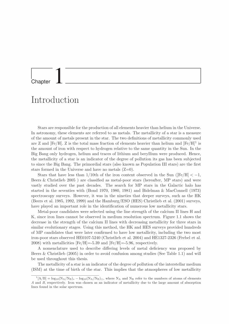
Metal-poor candidates were selected using the line strength of the calcium II lines H andK, since iron lines cannot be observed in medium resolution spectrum. Figure 1.1 shows thedecrease in the strength of the calcium II lines with decreasing metallicity for three stars insimilar evolutionary stages. Using this method, the HK and HES surveys provided hundredsof MP candidates that were later confirmed to have low metallicity, including the two mostiron-poor stars observed HE0107-5240 (Christlieb et al. 2004) and HE1327-2326 (Frebel et al.2008) with metallicities [Fe/H]=-5.39 and [Fe/H]=-5.96, respectively.
A nomenclature used to describe differing levels of metal deficiency was proposed byBeers & Christlieb (2005) in order to avoid confusion among studies (See Table 1.1) and willbe used throughout this thesis.
The metallicity of a star is an indicator of the degree of pollution of the interstellar medium(ISM) at the time of birth of the star. This implies that the atmospheres of low metallicity
1[A/B] = log10(NA/NB)∗ − log10(NA/NB)⊙, where NA and NB refer to the numbers of atoms of elementsA and B, respectively. Iron was chosen as an indicator of metallicity due to the large amount of absorptionlines found in the solar spectrum.
2 CHAPTER 1. INTRODUCTION
Figure 1.1: HES spectra of metal-poor stars found in the HK survey for different metallicities. Note thatwavelength is decreasing from left to right and the variation in the line strength of the calcium lines withmetallicity. Figure taken from Christlieb (2003). The labels in the upper part of each plot indicate: Thename of the star using the nomenclature of the HK/HES surveys. B is the magnitude in the Johnson’sfilter. TO indicates the evolutionary stage of the star, in this case Turnoff. [Fe/H] is the metallicity of thestar.
stars reflect the nucleosynthesis products of fewer stellar generations than the atmospheres ofthose stars more metal-rich. Extremely metal-poor stars, hereafter EMP stars, have less than
1.1. CEMP STARS 3
Term Acronym [Fe/H]
Super metal-rich SMR > +0.5Solar — ∼ 0.0
Metal-poor MP < −1.0Very metal-poor VMP < −2.0
Extremely metal-poor EMP < −3.0Ultra metal-poor UMP < −4.0Hyper metal-poor HMP < −5.0Mega metal-poor MMP < −6.0
Table 1.1: Nomenclature for star of different metallicities from Beers & Christlieb (2005)
1/1000th of the iron content of the sun (Table 1.1) and are an important key to understandthe chemical evolution of the Milky Way during its early stages. Their abundance patternsmight shed light on individual nucleosynthesis processes, contrary to those more metal-richstars, which reflect the well-mixed products of several nucleosynthesis processes in multiplegenerations of stars.
Several attempts have been made in order to explain the peculiarities of EMP abundancepatterns; their origin, nevertheless, is still an unsolved puzzle. One of the first scenarios pro-posed to explain the overabundance of carbon and nitrogen in EMP stars involved the inges-tion of protons into the helium convective zone (proton ingestion episode-PIE) that happensduring the core He-flash in Pop. III and EMP stars (Fujimoto et al. 1990; Schlattl et al. 2001;Weiss et al. 2004; Picardi et al. 2004). The proton ingestion into the helium-rich convectivelayers during the core He-flash is a robust phenomenon in one dimensional stellar evolution cal-culations of low metallicity stars ([Fe/H] < −4.5) that subsequently leads to a large surface en-richment in CNO-elements (Hollowell et al. 1990; Schlattl et al. 2001; Campbell & Lattanzio2008). However, the amount of C, N, and O dredged-up to the surface in the models is 1 to 3dex larger than the observed [C/Fe], disfavoring the self-enrichment scenario. Besides, mostEMP stars observed are not evolved past the helium-core flash to have undergone PIE.
1.1 CEMP stars
One import characteristic of EMP stars is the larger fraction of carbon-enhanced starscompared with those more metal-rich. While solar metallicity stars enriched in carbon repre-sent ∼ 1% of the total number of stars (Tomkin et al. 1989; Luck & Bond 1991), 20-30% ofthe stars with metallicity [Fe/H] < −2.5 are carbon enhanced (Rossi et al. 1999; Suda et al.2011). There is no agreement between studies in the quantitative definition of CEMP stars,however, the difference in the definition is not sufficient to disprove the larger fraction ofcarbon enrichment among EMP stars. This finding was originally observed in medium reso-lution spectroscopy studies, which prompted numerous high resolution spectroscopy follow-upobservations of carbon enhanced EMP stars in order to obtain detailed abundance patterns.
Carbon-enhanced metal-poor stars, known as CEMP stars, belong to a more complexclass than initially thought. These stars present a wide variety of patterns in terms of neutroncapture elements, with stars showing no signatures of these elements to others having large

4 CHAPTER 1. INTRODUCTION
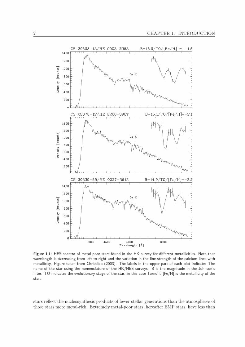
enhancement in s-process or r-process1 elements, or in both. Table 1.2 shows the CEMPstars subclasses (Beers & Christlieb 2005). Ba and Eu are mainly formed by s- and r-process,respectively. For this reason, they are used as tracers of each process and were chosen tocategorize the CEMP subclasses. Figure 1.2 shows the Ba and Eu abundances for the CEMPstars observed in high resolution. The abundances were taken from the SAGA database(Suda et al. 2008). As it can be seen, the Ba/Fe and Eu/Fe abundance ratios can be up tothree orders of magnitude larger than the ratios observed in the Sun. The stars enrichedonly in s-process elements tend to have lower [Ba/Fe] abundances than stars enriched in bothneutron capture processes.
Figure 1.2: Overview of the observational data for CEMP stars. Black symbols represent the CEMP-s stars,green symbols represent the CEMP-rs stars, and red symbols represent the CEMP-r stars according to theclassification of Masseron et al. (2010). Data points were taken from the SAGA database.
The majority of CEMP stars are enhanced in s-process elements (∼ 80% - Aoki et al.2008), being approximately equally distributed between CEMP-s and CEMP-rs stars. Thepositive correlation between carbon and s-process elements suggests that they might have thesame production site (Aoki et al. 2002; Suda et al. 2004, 2011). Figure 1 from Masseron et al.2010 shows that CEMP-s stars exhibit [Ba/Fe] and [Eu/Fe] ratios identical to classical Bastars. Qualitatively the origin of carbon and s-process elements in CEMP-s stars can beexplained by mass transfer from a AGB (Asymptotic Giant Branch) companion (now a whitedwarf).
1Elements heavier than iron are formed by neutron capture into iron-seeds elemends. The neutron captureprocesses are divided into two: s(low)-process and r(apid)-process.

1.1. CEMP STARS 5
Subclass
CEMP-r [Eu/Fe] > 1.0CEMP-s [Ba/Eu] > 0.5 & [Ba/Fe] > 1.0CEMP-rs 0.0 < [Ba/Eu] < 0.5CEMP-no [Ba/Fe] < 0.0
Table 1.2: Classification of CEMP stars as proposed by Beers & Christlieb (2005). The definition of a CEMPstar is the star with [C/Fe] > 1.0. The CEMP definition varies between different studies: [C/Fe] > 0.9according to Masseron et al. 2010, [C/Fe] > 0.7 according to Suda et al. 2011. The letter s stands fors-process elements, and the letter r stands for r-process elements.
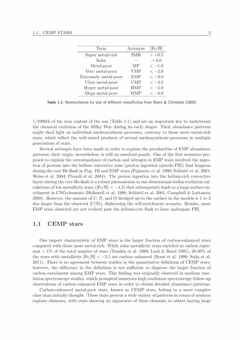
Mass would be transferred via stellar winds or via Lobe-Roche overflow and products ofAGB nucleosynthesis would be dumped onto the convective envelope of the observed star(Figure 1.3). Radial velocity monitoring has shown that a large fraction of CEMP-s starsexhibits radial velocity variations, strengthening the argument of a binary scenario for theformation of CEMP-s stars (Lucatello et al. 2005).
Figure 1.3: Mass Transfer in a binary system via Roche Lobe overflow. Adapted using the image of theSun by NASA.
Quantitative results for s-process nucleosynthesis were presented by Bisterzo et al. 2010.They have performed s-process calculations based on AGBmodels with masses M = 1.3− 2.0M⊙
and metallicities −3.6 ≤ [Fe/H] ≤ −1.0. In these models, neutrons are burnt radiatively in-side the 13C pocket. The 13C pocket was formulated as a region where the abundance of themain neutron source (13C) is larger than the abundance of the main neutron poison (14N).This region might form if protons from the bottom of the convective envelope penetrate theHe intershell after the third dredge-up and are captured by the abundant 12C (Gallino et al.1998). The physical mechanism reponsible for the formation of the 13C pocket is not yetestablished. For this reason, its efficiency is a free parameter in the models. Using differentefficiencies of the 13C pocket Bisterzo et al. 2011 are able to reproduce the general trend forthe s-process abundance patterns of CEMP stars.
Lugaro et al. (2012) presented models for the s-process in AGB stars of masses M = 0.9−6.0M⊙ and metallicity [Fe/H] = −2.3. In these models 13C is mainly burnt in radiativeconditions during the interpulse periods. Some models present mild proton ingestion, leading13C to burn in convective conditions during the thermal pulse. The inclusion of the 13Cpocket was done by forcing the code to mix a small amount of proton from the envelope into

6 CHAPTER 1. INTRODUCTION
the intershell. The proton abundance decreases from 0.7 in the envelope to 10−4 at a givenpoint in mass located bellow the bottom of the envelope. The free parameter in the modelsis the mass between the bottom of the envelope and the point where the proton abundanceis 10−4. Models with masses M ∼ 2M⊙, where
13C burns radiatively, produce a good matchto the CEMP-s stars.
Suda et al. (2004) argued that the most likely production site for carbon and s-processelements is the PIE during the AGB phase of stars with mass 1.2M⊙ < M ≤ 3.0M⊙ andmetallicities [Fe/H] ≤ −2.5. At the beginning of the AGB evolution, protons are dredged-down into the helium convective zone due to the low entropy barrier between the H- and He-rich layers. Neutrons are produced in a convective environment via 13C(α, n)16O. The highneutron densities achieved during the PIE (Nn > 1013cm−3) can lead to a large productionof s-process elements. This phenomenon, that only happens in an extremely low metallicityenvironment in the 1D stellar evolution models, was not taken into account in Bisterzo et al.(2010) simulations. For metallicities [Fe/H] < −2.5 they used an extrapolated stellar structurefrom more metal-rich models. Therefore, more realistic models, taking PIE into account, forthe nucleosynthesis during the AGB evolution of EMP stars are still missing in the literature.
1.2 The most iron-poor stars
The two hyper metal-poor stars (see Table 1.1) discovered to date (HE0107-5240 andHE1327-2326) have been subject of extensive theoretical and observational studies. Bothstars are strongly enhanced in carbon, nitrogen and oxygen, despite their extremely low ironcontent. The exact CEMP class they belong to, however, is not yet determined since thereare only upper limits values for the Ba and Eu abundances (Table 1.3).
Element HE0107-5240 HE1327-2326
[Fe/H] −5.39 −5.96[C/Fe] 3.70 3.78[N/Fe] 2.28 4.28[O/Fe] 2.30 3.42[Na/Fe] 0.81 2.73[Mg/Fe] 0.15 1.97[Al/Fe] < −0.26 1.46[Ti/Fe] -0.36 0.91[Sr/Fe] < −0.52 1.17[Ba/Fe] < 0.82 < 1.40[Eu/Fe] < 2.78 < 4.64
Table 1.3: Relative abundances of HE0107-5240 (Bessell et al. 2004; Christlieb et al. 2004) and HE1327-2326 (Frebel et al. 2008).
The first question that rises from the observations is whether the carbon, nitrogen, andoxygen enhancements are the result of external pollution or internal processes. HE1327-2326is an unevolved star, which exclude the possibility for a self-pollution scenario since the bottomof the convective envelope only reaches the ashes of burning regions when the star becomes a
1.3. PRIMORDIAL STARS 7
giant. On the other hand, HE0107-5240 is a giant star. Nevertheless, comparisons betweenits position in the (log g,log Teff) plane and theoretical tracks, have shown that it is far fromthe tip of the red giant branch, where the proton ingestion occurrs, and thus could not haveyet produced the CNO elements observed in its atmosphere (Picardi et al. 2004; Weiss et al.2004).
Therefore, other interpretations for the abundance patterns of HMP stars remain: 1) Theyare second generation stars and their photosphere reflects only the nucleosynthetic yields ofPop. III supernovae; 2) they are primordial stars which accreted material after their birthfrom the primordial cloud or their abundance patterns are the result of mass-transfer froma companion; 3) they are primordial or second generation stars which acquired most of theirmetals from the Galactic ISM.
Iwamoto et al. (2005) presented Pop. III supernovae yields for stars with initial massM = 25M⊙. Their models can reproduce the overabundance of CNO elements in the HMPstars. Heger & Woosley (2010) also performed supernovae nucleosynthesis calculation ofmetal-free stars with initial masses in the range 10− 100M⊙. The best fits to HE1327-2326and HE0107-5240 abundances were obtained for low energy explosions models and stars inthe mass range 10− 30M⊙. These results reinforce prior suggestions that primordial starswere formed with smaller masses.
Suda et al. (2004) discussed the possibility that HE0107-5240 is a primordial star thatwas polluted by CNO and s-process elements via mass-transfer from an AGB companion. Intheir scenario, the atmosphere of the stars in the binary system would be polluted in iron-peak elements via accretion of gas from the polluted primordial cloud. CNO and s-processelements would be formed during the PIE occurring at the beginning of the TP-AGB in theprimary star and later dumped onto HE0107-5240 atmosphere. They have shown that thebinary scenario is a viable possibility if HE0107-5240 is either a first or a second generationstar and its companion has an initial mass in the range 1.2 ≤ M/M⊙ ≤ 3.0. They have foundthat C, N, O, Na, and Mg can be produced during the PIE and, if iron-peak elements arepresent in the convective zone, s-process elements might also be formed. In order to determinewhether HE0107-5240 is a first or a second generation star accurate measurements of s-processelements are necessary. In addition, recent nucleosynthesis model by Campbell et al. (2010)have shown that s-process production might happen also during the core He-flash, contra-dicting Fujimoto et al. (2000) results, and thus, low-mass stars might also be responsible forthe abundance pattern observed in the HMP stars.
1.3 Primordial Stars
The nature of the primordial stars has been subject of intensive debate. It was a generalidea that the metal-free environment could form only isolated stars with extremely largemasses (Abel et al. 2002; Bromm et al. 2002; Bromm & Loeb 2004; O’shea & Norman 2007;Yoshida et al. 2008), since the cooling efficiency would be small due to the absence of metals.
Star formation depends on the competition between gravity and outwards forces (pressuregradient, magnetic fields, and turbulance). The mass distribution of the stars formed, i.e. theinitial mass function - IMF, is controlled by the heating and cooling processes in the gas.Metals are responsible for most of the cooling in the present-day molecular clouds, decreasingtheir temperature down to T ∼ 10 K. Metal atoms, excited by collisions, return to a lower

8 CHAPTER 1. INTRODUCTION
energy state by emitting a photon which, in turn, can leave the region, cooling the cloud.Nevertheless, in primordial clouds where there are no metals, cooling is produced by H2
molecules which reduces the cloud temperature to T = 100− 200 K.The minimum mass that a cloud of gas must have to collapse under its gravity is called
the Jeans mass:
MJ = 45M⊙T3/2n
−1/2H , (1.1)
where T is the temperature in kelvins and nH is the hydrogen density given in cm−3.
Based on the above equation, it can be seen that the primordial stars should be moremassive than M > 100M⊙. Contrary, the observed Populations I and II stars have muchlower masses M < 1.0M⊙. The transition between these two modes of star formation shouldbe mainly controlled by the increasing metallicity which is an indicative that there should bea critical metallicity, Zc below which only massive stars were formed. Bromm & Loeb (2003)argued that since the two main coolants in the cloud are oxygen and carbon, the two modes ofstar formation should be separated by the critical abundances of these two elements, insteadof a critical total metallicity. They found that all low metallicity stars observed at the timehad larger oxygen abundance than the critical oxygen value, although some stars presentedsubcritical carbon abundance. This subcritical carbon abundance could be formed post-birth during the RGB phase, therefore, it would not invalidate their argument. However, therecent discovery of an EMP star with metallicity [Fe/H] = −4.89 and no enhancement in CNOelements (Caffau et al. 2011, 2012), which results in the lowest total metallicity Z ≤ 10−4Z⊙
observed in a star, puts into question the claims of a minimum metallicity required for theformation of low-mass stars.
One important mechanism to form low-mass stars is the fragmentation of large cloudsinto smaller collapsing clumps. Fragmentation occurs if the free-fall compressional heatingrate is smaller than the radiative cooling rate. Old numerical simulations of metal-free starformation have found no fragmentation which led to the general idea that Pop. III starswere isolated systems. These simulations were limited to a narrow timespan and the possibleformation and fragmentation of a circumstellar disc could not be followed. Recent simulations,employing sink particles to represent the growing protostars, found strong fragmentation inthe protostellar disc due to a very efficient cooling by H2 lines and collision-induced emission(Stacy et al. 2010, 2012; Greif et al. 2011). They have shown that Pop. III stars can beformed in multiple systems with a flat protostellar mass function (M ∼ 0.1− 10M⊙). Thesink particle approach is subjected to a large inaccuracy. The mass function derived usingthis approach is quite uncertain. Nonetheless, the occurrence of fragmentation found in thesimulations shows that low-mass metal-free stars could be formed.
1.4 Outline
We focused on the study of the nucleosynthesis of stars with metallcities [Fe/H] < −3.0.In all these stars proton ingestion takes place, either during the core He-flash or the TP-AGB phase. The goal of this thesis is to study the s-process production during the proton

1.4. OUTLINE 9
ingestion and its contribution to the abundance patterns observed in EMP stars. We explorethe uncertainties in modelling such phenomenon and the AGB phase.
The thesis is structured as follows: In Chapter 2 we give an overview of stellar evolutionand nucleosynthesis. Also, we give a literature overview of the proton ingestion episode andits characteristics. In Chapter 3 we give a brief overview of the evolutionary code, the inputphysics used in the models, and the modifications performed to the code. In Chapter 4 wegive an overview of the post-processing code created for the purpose of this thesis. In Chapter5 we presented our low-mass stars models and their influence on the HMP stars abundancepatterns. In Chapter 6 we presented our intermediate-mass stars models. In Chapter 7 weuse the extended network in the evolutionary code to understand the abundance anomaliesin Globular Clusters. Finally in Chapter 8 we present the conclusions.

10 CHAPTER 1. INTRODUCTION

Chapter 2On the Evolution of Moderate-Mass stars
The evolution of a star is strongly dependent on its initial mass. Throughout the course of itslife, a star undergoes many evolutionary stages, amongst them, the Asymptotic Giant Branch,referred to as AGB phase. The AGB phase is the production site of heavy elements. In thischapter a sketch of the evolution prior and during the AGB phase will be discussed, togetherwith a brief discussion on the formation of s-process elements. For a more detailed descriptionwe refer the reader to the standard textbooks: Clayton (1983), Kippenhahn & Weigert (1990).

12 CHAPTER 2. ON THE EVOLUTION OF MODERATE-MASS STARS
2.1 Introduction
Stars classified as moderate-mass stars are those ending their lives as white dwarfs. Theyare divided into low- and intermediate-mass stars. This classification is based on the wayhelium is burnt in the core, if in a violent (He-flash) or a quiescent way. The mass boundarybetween low- and intermediate-mass stars is model and metallicity dependent. In general,stars with mass below 2M⊙ experience core He-flash and are classified as low-mass stars.Stars with masses between 2M⊙ and 10M⊙ are classified as intermediate-mass stars.
A protostar of mass larger than 0.08M⊙ will reach high enough temperatures in the centerto start fusion and become a zero-age main sequence (ZAMS) star. In the ZAMS phase thestar is assumed to be chemically homogenous and in equilibrium. The evolution at this pointstrongly depends on the stellar mass and will be described in 2.2.
As the star advances in the evolution, it assumes more and more an onion-like structure,with shells powered by different burning mechanisms on top of each other. In the AGBphase, for instance, the core is surrounded by He- and H-burning shells. The structure andnucleosynthesis of this evolutionary stage will be discussed in 2.3 and 2.4. 2.4 will focus onthe formation of elements heavier than iron and its connection with the AGB phase.
2.2 Evolution pre-AGB phase
2.2.1 Low-Mass Stars
The main-sequence (MS) phase begins at the ZAMS and finishes when hydrogen is ex-hausted in the center, and corresponds to the majority of the stellar life. During the MSof low-mass stars, H-burning is dominated by the proton-proton (pp) chain reactions in aradiative core (for M ≥ 1.1M⊙ a convective core develops due to the increasing importanceof the CNO cycle (Figure 2.1)). The pp chain, as can be seen in the panel (a) of Figure2.1, involves the fusion of two protons into a deuterium, leading to the formation of heliumvia three different branches (PPI, PPII, PPIII). The frequency of the branches depends onchemical compositon, temperature, and density.
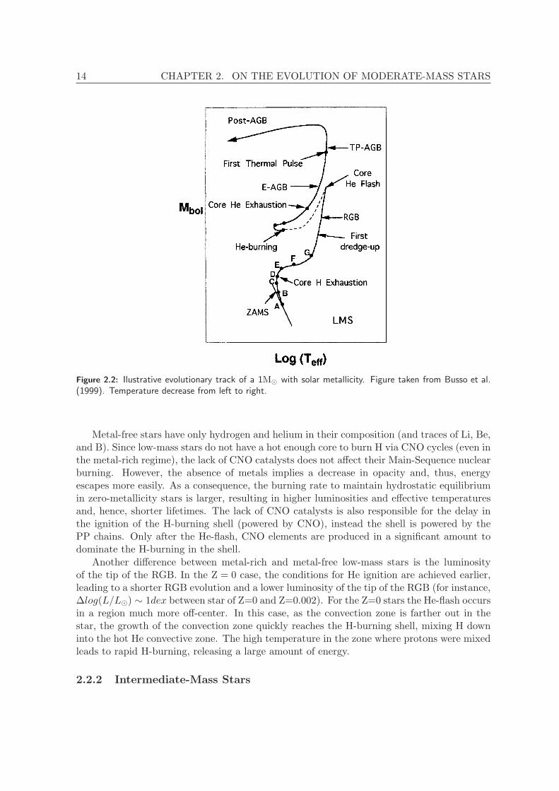
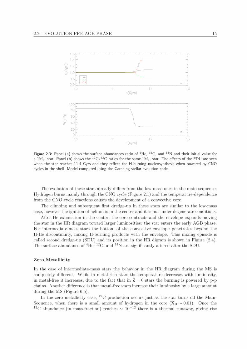
Figure 2.2 illustrates the evolution of a low-mass star in the Hertzsprung-Russel diagram(HRD). The MS is represented by the points A to D. The point where the star leaves the MSafter the exhaustion of hydrogen in the core is the turn-off point (point D in Figure 2.2). Fromthe turn-off point onwards, the energy source is H-burning (dominated by the CNO cycle)in a shell around the inert helium core. The envelope start expanding as a reaction to thecontraction of the core. The star enters the subgiant phase (points E to G in Figure 2.2) andmoves towards lower temperature in the HRD. The cooling of the stellar outer layers results inthe formation of a convective envelope. The star moves towards lower effective temperaturesand higher luminosities in the HR diagram. As the star climbs the giant branch, the convectiveenvelope penetrates deeply inwards and material partially processed by H-burning is broughtto the surface. This event, known as first dredge-up (FDU), results in an increase of theabundances of isotopes such as 4He, 13C, and 14N (formed through the activation of the CNOcycles) and in a decrease of 12C abundances (Figure 2.3). The decrease in the 12C/13C ratiois shown in panel (b) of Figure 2.3 and can be used to trace the FDU since 12C is present in

2.2. EVOLUTION PRE-AGB PHASE 13
Figure 2.1: Panel (a) shows the reactions involved in the pp chain. The energies released by the branchesare: 26.2 MeV (PPI), 25.7 MeV (PPII), and 19.2 MeV (PPIII). Panel (b) shows the reactions involved inthe CNO cycles. The elements C, N , and O act as catalysts in these reactions. Their final abundances arethose of equilibrium in the CNO cycles and the sum of these abundances is equal to the sum of the initialvalues.
the photosphere of MS stars, whilst 13C is only present after products of the CNO cycle aredredged-up to the surface via convective mixing.
The core continues to contract while the star climbs the red giant branch (RGB) and atsome point the core becomes dense enough to be degenerate. When the temperature is hotenough, He is burnt off-center in a violent way (core He-flash), as a result of the decouplingof temperature and density in the equation of state of the degenerate matter. The increasein temperature in the core is not compensated by its expansion and subsequent cooling. Inthis way, the energy released by nuclear burning heats up the core, which in turn will increasethe reaction rates, until a thermonuclear runaway occurs. The off-center nature of the coreHe-flash is a result of neutrino energy loss, which cools the core in the hot and dense regions.The cooling efficiency decreases with density, leading to a higher temperature on the borderof the cooled region.
After the He ignition the star moves in the HR diagram to higher temperatures and lowerluminosities. Now, the core He-burning is surrounded by a H-burning shell. If the star hassolar metallicity it is in a position in the HR diagram called red giant clump, on the otherhand if it has lower metallicity it is on the horizontal branch (HB). After He exhaustion inthe center the core starts to contract and the envelope expands. Helium is now burning in ashell surrounded by the H-burning shell and the star ascends again the giant branch (AGB)phase.
Zero Metallicity
For primordial stars the evolution can be quite different compared to the evolution of themetal-rich ones and even from the Population II case.
14 CHAPTER 2. ON THE EVOLUTION OF MODERATE-MASS STARS
Figure 2.2: Ilustrative evolutionary track of a 1M⊙ with solar metallicity. Figure taken from Busso et al.(1999). Temperature decrease from left to right.
Metal-free stars have only hydrogen and helium in their composition (and traces of Li, Be,and B). Since low-mass stars do not have a hot enough core to burn H via CNO cycles (even inthe metal-rich regime), the lack of CNO catalysts does not affect their Main-Sequence nuclearburning. However, the absence of metals implies a decrease in opacity and, thus, energyescapes more easily. As a consequence, the burning rate to maintain hydrostatic equilibriumin zero-metallicity stars is larger, resulting in higher luminosities and effective temperaturesand, hence, shorter lifetimes. The lack of CNO catalysts is also responsible for the delay inthe ignition of the H-burning shell (powered by CNO), instead the shell is powered by thePP chains. Only after the He-flash, CNO elements are produced in a significant amount todominate the H-burning in the shell.
Another difference between metal-rich and metal-free low-mass stars is the luminosityof the tip of the RGB. In the Z = 0 case, the conditions for He ignition are achieved earlier,leading to a shorter RGB evolution and a lower luminosity of the tip of the RGB (for instance,∆log(L/L⊙) ∼ 1dex between star of Z=0 and Z=0.002). For the Z=0 stars the He-flash occursin a region much more off-center. In this case, as the convection zone is farther out in thestar, the growth of the convection zone quickly reaches the H-burning shell, mixing H downinto the hot He convective zone. The high temperature in the zone where protons were mixedleads to rapid H-burning, releasing a large amount of energy.
2.2.2 Intermediate-Mass Stars
2.2. EVOLUTION PRE-AGB PHASE 15
Figure 2.3: Panel (a) shows the surface abundances ratio of 4He, 12C, and 14N and their initial value fora 1M⊙ star. Panel (b) shows the 12C/13C ratios for the same 1M⊙ star. The effects of the FDU are seenwhen the star reaches 11.4 Gyrs and they reflect the H-burning nucleosynthesis when powered by CNOcycles in the shell. Model computed using the Garching stellar evolution code.
The evolution of these stars already differs from the low-mass ones in the main-sequence:Hydrogen burns mainly through the CNO cycle (Figure 2.1) and the temperature-dependencefrom the CNO cycle reactions causes the development of a convective core.
The climbing and subsequent first dredge-up in these stars are similar to the low-masscase, however the ignition of helium is in the center and it is not under degenerate conditions.
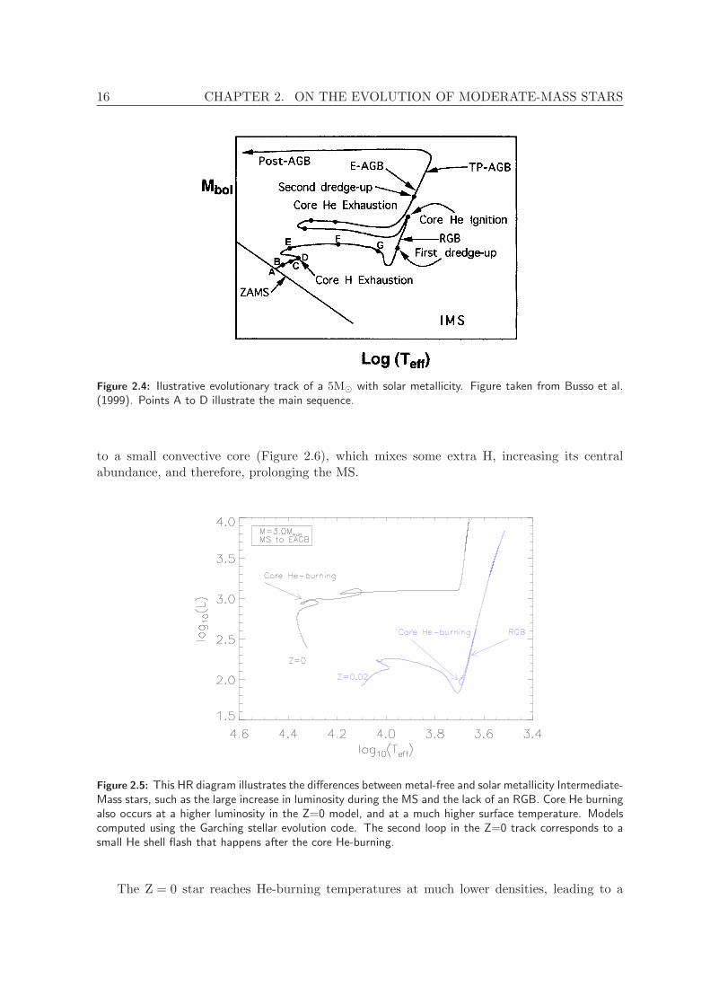
After He exhaustion in the center, the core contracts and the envelope expands movingthe star in the HR diagram toward larger luminosities: the star enters the early AGB phase.For intermediate-mass stars the bottom of the convective envelope penetrates beyond theH-He discontinuity, mixing H-burning products with the envelope. This mixing episode iscalled second dredge-up (SDU) and its position in the HR digram is shown in Figure (2.4).The surface abundance of 4He, 12C, and 14N are significantly altered after the SDU.
Zero Metallicity
In the case of intermediate-mass stars the behavior in the HR diagram during the MS iscompletely different. While in metal-rich stars the temperature decreases with luminosity,in metal-free it increases, due to the fact that in Z = 0 stars the burning is powered by p-pchains. Another difference is that metal-free stars increase their luminosity by a large amountduring the MS (Figure 6.5).
In the zero metallicity case, 12C production occurs just as the star turns off the Main-Sequence, when there is a small amount of hydrogen in the core (XH ∼ 0.01). Once the12C abundance (in mass-fraction) reaches ∼ 10−12 there is a thermal runaway, giving rise
16 CHAPTER 2. ON THE EVOLUTION OF MODERATE-MASS STARS
Figure 2.4: Ilustrative evolutionary track of a 5M⊙ with solar metallicity. Figure taken from Busso et al.(1999). Points A to D illustrate the main sequence.
to a small convective core (Figure 2.6), which mixes some extra H, increasing its centralabundance, and therefore, prolonging the MS.
Figure 2.5: This HR diagram illustrates the differences between metal-free and solar metallicity Intermediate-Mass stars, such as the large increase in luminosity during the MS and the lack of an RGB. Core He burningalso occurs at a higher luminosity in the Z=0 model, and at a much higher surface temperature. Modelscomputed using the Garching stellar evolution code. The second loop in the Z=0 track corresponds to asmall He shell flash that happens after the core He-burning.
The Z = 0 star reaches He-burning temperatures at much lower densities, leading to a

2.2. EVOLUTION PRE-AGB PHASE 17
quiet ignition of He in the core. The star rapidly changes from core H-burning to core He-burning, avoiding a RGB configuration. Due to the lack of RGB, only one mixing episodeoccurs. The envelope goes deeply enough to reach regions that have been subjected to partialhydrogen burning. However, once the H-burning occurs via p-p chain the envelope is notenriched in 14N as it occurs in the metal-rich regime and, also, the enrichment in 4He is muchstronger (Figure 2.7).
Figure 2.6: Mass fraction of hydrogen in the core as a function of time for a metal-free star. The developmentof the convective core can be seen by the increase in the mass fraction towards the end of the MS. Modelscomputed using the Garching stellar evolution code.
18 CHAPTER 2. ON THE EVOLUTION OF MODERATE-MASS STARS
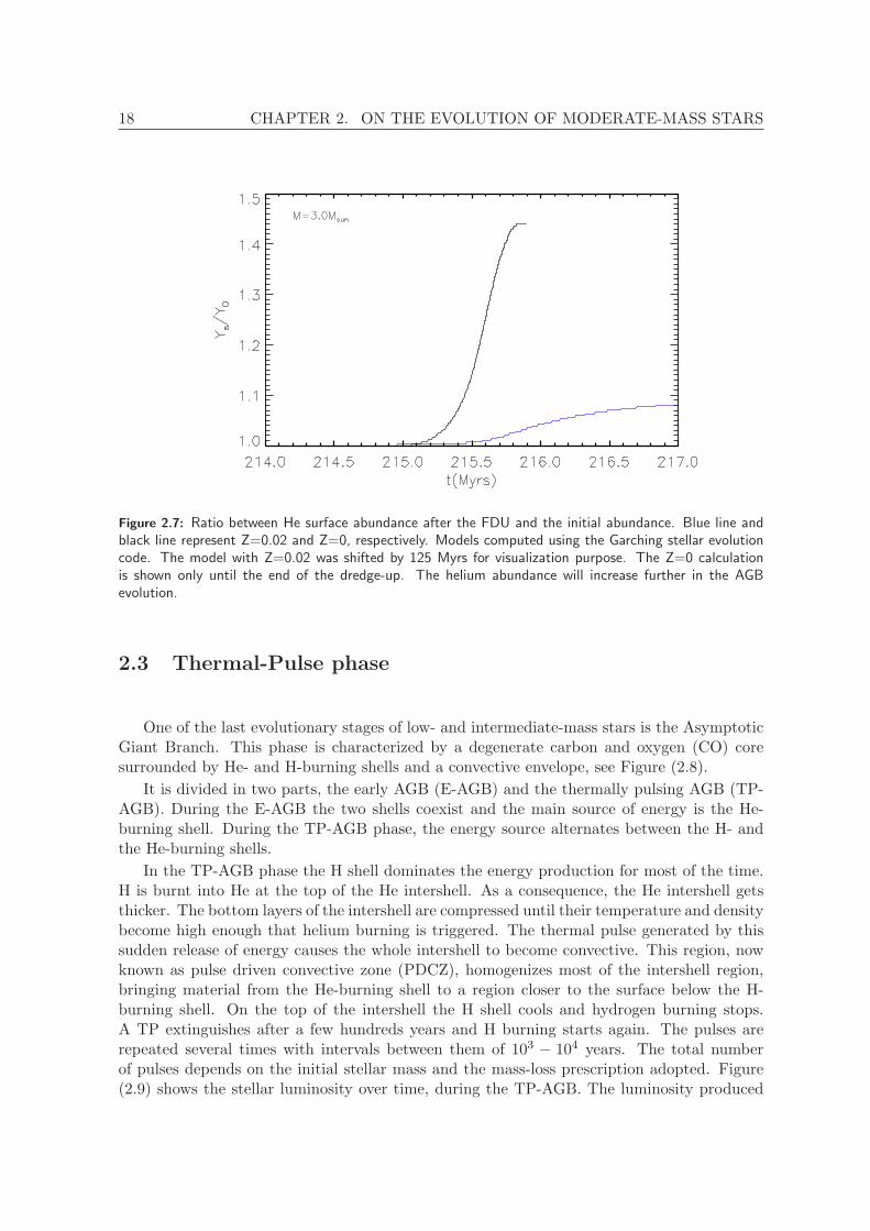
Figure 2.7: Ratio between He surface abundance after the FDU and the initial abundance. Blue line andblack line represent Z=0.02 and Z=0, respectively. Models computed using the Garching stellar evolutioncode. The model with Z=0.02 was shifted by 125 Myrs for visualization purpose. The Z=0 calculationis shown only until the end of the dredge-up. The helium abundance will increase further in the AGBevolution.
2.3 Thermal-Pulse phase
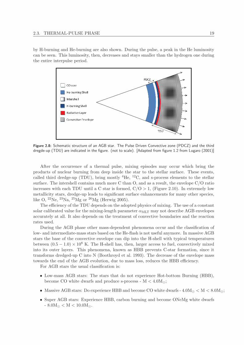
One of the last evolutionary stages of low- and intermediate-mass stars is the AsymptoticGiant Branch. This phase is characterized by a degenerate carbon and oxygen (CO) coresurrounded by He- and H-burning shells and a convective envelope, see Figure (2.8).
It is divided in two parts, the early AGB (E-AGB) and the thermally pulsing AGB (TP-AGB). During the E-AGB the two shells coexist and the main source of energy is the He-burning shell. During the TP-AGB phase, the energy source alternates between the H- andthe He-burning shells.
In the TP-AGB phase the H shell dominates the energy production for most of the time.H is burnt into He at the top of the He intershell. As a consequence, the He intershell getsthicker. The bottom layers of the intershell are compressed until their temperature and densitybecome high enough that helium burning is triggered. The thermal pulse generated by thissudden release of energy causes the whole intershell to become convective. This region, nowknown as pulse driven convective zone (PDCZ), homogenizes most of the intershell region,bringing material from the He-burning shell to a region closer to the surface below the H-burning shell. On the top of the intershell the H shell cools and hydrogen burning stops.A TP extinguishes after a few hundreds years and H burning starts again. The pulses arerepeated several times with intervals between them of 103 − 104 years. The total numberof pulses depends on the initial stellar mass and the mass-loss prescription adopted. Figure(2.9) shows the stellar luminosity over time, during the TP-AGB. The luminosity produced
2.3. THERMAL-PULSE PHASE 19
by H-burning and He-burning are also shown. During the pulse, a peak in the He luminositycan be seen. This luminosity, then, decreases and stays smaller than the hydrogen one duringthe entire interpulse period.
Figure 2.8: Schematic structure of an AGB star. The Pulse Driven Convective zone (PDCZ) and the thirddregde-up (TDU) are indicated in the figure. (not to scale). [Adapted from figure 1.2 from Lugaro (2001)]
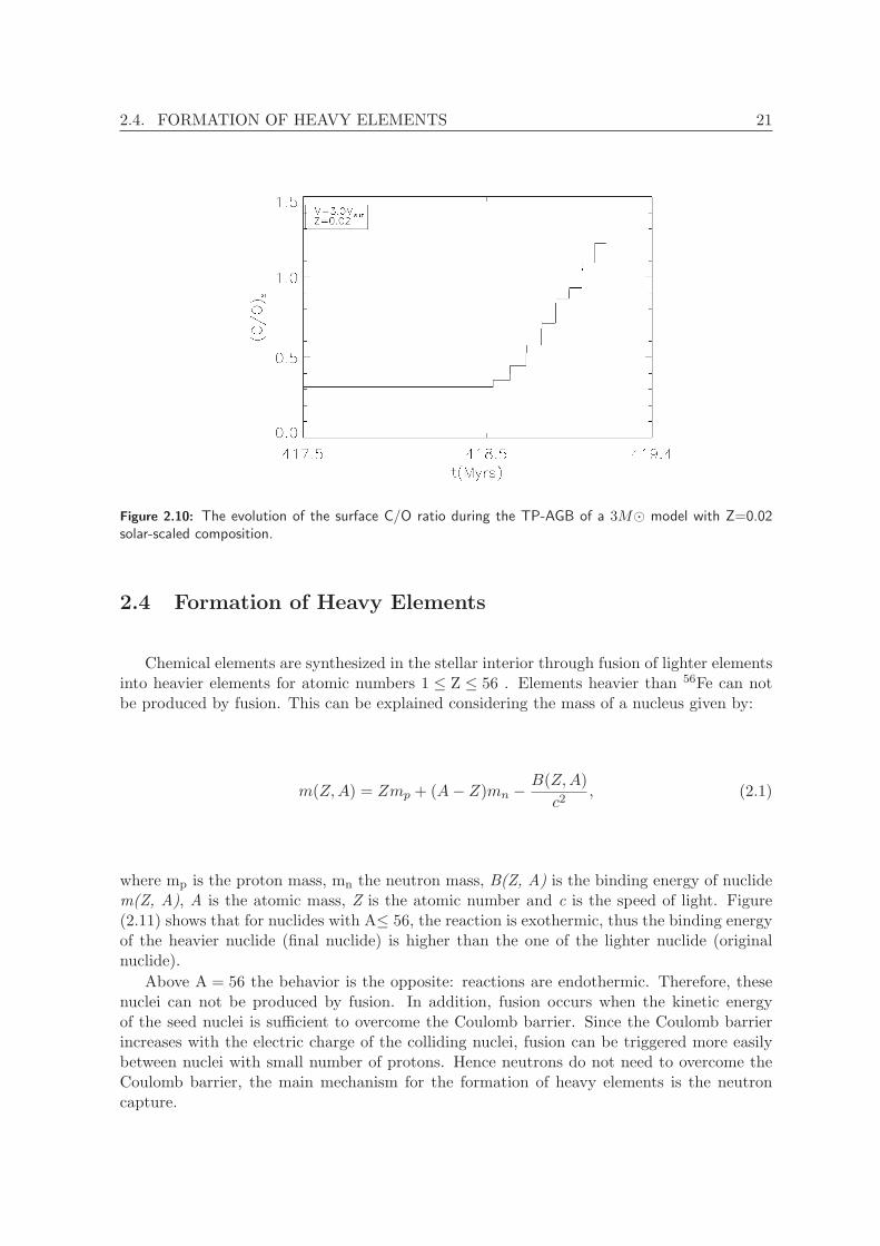
After the occurrence of a thermal pulse, mixing episodes may occur which bring theproducts of nuclear burning from deep inside the star to the stellar surface. These events,called third dredge-up (TDU), bring mostly 4He, 12C, and s-process elements to the stellarsurface. The intershell contains much more C than O, and as a result, the envelope C/O ratioincreases with each TDU until a C star is formed, C/O > 1, (Figure 2.10). In extremely lowmetallicity stars, dredge-up leads to significant surface enhancements for many other species,like O, 22Ne, 23Na, 25Mg or 26Mg (Herwig 2005).
The efficiency of the TDU depends on the adopted physics of mixing. The use of a constantsolar calibrated value for the mixing-length parameter αMLT may not describe AGB envelopesaccurately at all. It also depends on the treatment of convective boundaries and the reactionrates used.
During the AGB phase other mass-dependent phenomena occur and the classification oflow- and intermediate-mass stars based on the He-flash is not useful anymore. In massive AGBstars the base of the convective envelope can dip into the H-shell with typical temperaturesbetween (0.5− 1.0)× 108 K. The H-shell has, then, larger access to fuel, convectively mixedinto its outer layers. This phenomena, known as HBB prevents C-star formation, since ittransforms dredged-up C into N (Boothroyd et al. 1993). The decrease of the envelope masstowards the end of the AGB evolution, due to mass loss, reduces the HBB efficiency.
For AGB stars the usual classification is:
• Low-mass AGB stars: The stars that do not experience Hot-bottom Burning (HBB),become CO white dwarfs and produce s-process - M < 4.0M⊙;
• Massive AGB stars: Do experience HBB and become CO white dwarfs - 4.0M⊙ < M < 8.0M⊙;
• Super AGB stars: Experience HBB, carbon burning and become ONeMg white dwarfs- 8.0M⊙ < M < 10.0M⊙.

20 CHAPTER 2. ON THE EVOLUTION OF MODERATE-MASS STARS
Figure 2.9: The evolution on the surface luminosity (red line) as a function of time for a 3M⊙ modelcomputed with the Garching stellar evolution code. Blue line: Luminosity of He-burning shell. Black Line:Luminosity of H-burning shell.
The nucleosynthesis signature of HBB includes Li production, high N abundances, lowC/O and 12C/13C ratios and enhancements of 23Na, 25Mg, 26Mg and 26Al (Ventura et al. 2002;Karakas & Lattanzio 2003; Denissenkov & Herwig 2003; Karakas & Lattanzio 2007; Karakas2010).
The initial-mass boundary for HBB depends on metallicity. Forestini & Charbonnel(1997) find HBB for M ≥ 5.0 for Z=0.02, while Siess et al. (2002) found HBB down to 3M⊙
for zero metallicity stars. In fact, the initial-mass boundary for low-metallicity stars is stillmodel dependent: Campbell & Lattanzio (2008) found HBB in zero metallicities stars forM ≥ 2.0M⊙ in contrast to Lau et al. (2009), whose models with M < 4.0M⊙ do not experi-ence HBB.
2.4. FORMATION OF HEAVY ELEMENTS 21
Figure 2.10: The evolution of the surface C/O ratio during the TP-AGB of a 3M⊙ model with Z=0.02solar-scaled composition.
2.4 Formation of Heavy Elements
Chemical elements are synthesized in the stellar interior through fusion of lighter elementsinto heavier elements for atomic numbers 1 ≤ Z ≤ 56 . Elements heavier than 56Fe can notbe produced by fusion. This can be explained considering the mass of a nucleus given by:
m(Z,A) = Zmp + (A− Z)mn −B(Z,A)
c2, (2.1)
where mp is the proton mass, mn the neutron mass, B(Z, A) is the binding energy of nuclidem(Z, A), A is the atomic mass, Z is the atomic number and c is the speed of light. Figure(2.11) shows that for nuclides with A≤ 56, the reaction is exothermic, thus the binding energyof the heavier nuclide (final nuclide) is higher than the one of the lighter nuclide (originalnuclide).
Above A = 56 the behavior is the opposite: reactions are endothermic. Therefore, thesenuclei can not be produced by fusion. In addition, fusion occurs when the kinetic energyof the seed nuclei is sufficient to overcome the Coulomb barrier. Since the Coulomb barrierincreases with the electric charge of the colliding nuclei, fusion can be triggered more easilybetween nuclei with small number of protons. Hence neutrons do not need to overcome theCoulomb barrier, the main mechanism for the formation of heavy elements is the neutroncapture.

22 CHAPTER 2. ON THE EVOLUTION OF MODERATE-MASS STARS
Figure 2.11: Binding energy per nucleon as a function of atomic mass.
The neutron capture process can be slow (s-process) or rapid (r-process) relative to thebeta decay rate1. The occurrence of one or another process depends on physical parameters,such as temperature and neutron density, which are closely connected to the evolutionarystage.
In the s-process stable isotopes are produced along the valley of beta stability, whereas inthe r-process neutron-rich atomic nuclei are created (Figure 2.12).
Figure 2.12: S-process and r-process paths. Black symbols represent stable iso-topes, green and yellow symbols represent unstable ones. Figure taken from:http : //www − alt.gsi.de/fair/overview/research/nuclear− structuree.html.
1The decay β− is the transformation of a neutron into a proton (which remains in the nucleus), an electron(which is ejected), and an anti neutrino, as described by the reaction: (Z,A) → (Z + 1, A) + e− + νe.
2.4. FORMATION OF HEAVY ELEMENTS 23
2.4.1 S-process
The s-process is characterized by a slow neutron capture, i.e, the average rate of neutroncapture by a certain nucleus is much smaller than the β decay rate. It is estimated that, inaverage, 102 − 105 years may pass between successive neutrons captures. This process is alsocharacterized by a neutron density of the order of 105 − 1011ncm−3 , which can be providedby two astrophysical sites:
• Core He-burning in massive stars, where the main neutron source is given by the reaction(2.2)
22Ne+4 He → 25Mg + n; (2.2)
• The He-shell in the AGB phase, during the thermal pulses, where the main neutronsource is the following reaction:
13C +4 He → 16O + n. (2.3)
The main products of the s-process are: Sr-Y-Zr, Ba-La-Ce-Pr-Nd and Pb, correspondingto its three largest abundance peaks. The reason for the existence of these three peaks lies inthe fact that for number of neutrons N = 50, 82, 126 the neutron capture cross-sections aremuch smaller than for other N. These “magic numbers” of neutrons are a quantum effect ofclosed shells in the same way that electrons in complete shells produce high chemical stabilityfor noble gases.
2.4.2 Classical Model and The S-process Components
In the classical model, the formation of s-process elements happens in a chain, startingwith iron seed nuclei. The changes in the abundances Ni over time are given by equation 2.4,where τ is the neutron exposure1 (which is the integral of the flux over time) and σi is theneutron capture cross-section by isotope i.
dNi
dτ= σi−1Ni−1 − σiNi, 56 ≤ i ≤ 209. (2.4)
In a steady state, dNi/dτ = 0 , the product σN is constant. Clayton et. al 1961 showedthat a simple neutron exposure τ can not reproduce the abundances of elements in the so-lar system. However, a good adjustment of σN for the solar system is obtained when anexponential distribution for the neutron expositions is assumed (Seeger et al. 1965):
1τ =∫vTNn(t)dt, where vT is the thermal velocity and Nn(t) is the neutron density

24 CHAPTER 2. ON THE EVOLUTION OF MODERATE-MASS STARS
ρ(τ) =GN56
τ0e−
ττ0 , (2.5)
where τ0 is the mean neutron exposure, G is the iron fraction exposed to neutrons and N56
is the initial 56Fe abundance.The curve σN decreases slowly with the mass number, once the product τ0σi increases
with it. However, when σ is very small (in the magic numbers), there is a sudden drop in thecurve. This effect is shown in Figure (2.13).
The exponential distribution of neutron exposures in equation (2.5) can reproduce thesolar abundances if three values of τ0 are adopted. These values depend on the atomic massA and are often referred to as s-process components. The main component is responsiblefor the production of isotopes in the atomic mass range 90 < A < 204. A good fit for thesolar abundances in this atomic range is obtained with τ0 ≈ 0.30mb−1.The weak component(A ≤ 90), which most likely environment is the core of massive stars (M ≥ 10M⊙) nicely fitsthe solar curve if τ0 ≃ 0.06mb−1 (Meyer 1994). It was also proposed the existence of a strongcomponent (204 < A < 209) in order to reproduce more than 50% of solar Lead abundance208Pb (Kappeler et al. 1989). In this case τ0 = 7.0mb−1.
Figure 2.13: Solar s-process σiNi distribution. The curve was obtained with an exponential distribution ofneutron exposures. Figure taken from Seeger et al. (1965).
In the classical model, no hypotheses on the s-process site were formulated. Ulrich (1973)proposed the pulse driven convective zone in the TP-AGB phase as the astrophysical site fors-process production. An exponential distribution of neutron exposures would be achieved by
2.4. FORMATION OF HEAVY ELEMENTS 25
the recurrent TPs, in agreement with the classical model assumption. However Straniero et al.(1995) demonstrated that the 13C(α, n)16O reaction is burning in radiative conditions dur-ing the interpulse period. In this case, the distribution of neutrons exposures changes andthe resulting distribution is a superposition of a few single exposures. The limitations ofthe classical model were revealed with improved new studies and therefore, the necessityof s-process calculations considering its possible sites. For this purpose, full stellar evolutionmodels are required, becoming the usual approach nowadays when performing s-process calcu-lations. S-process calculations are performed, in general, in a post-processing code which usesthe thermodynamic output from the full evolutionary models as the input for the s-processnetwork.
2.4.3 The 13C Pocket
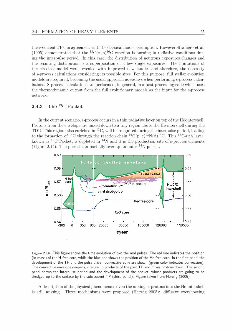
In the current scenario, s-process occurs in a thin radiative layer on top of the He-intershell.Protons from the envelope are mixed down to a tiny region above the He-intershell during theTDU. This region, also enriched in 12C, will be re-ignited during the interpulse period, leadingto the formation of 13C through the reaction chain 12C(p, γ)13N(β)13C. This 13C-rich layer,known as 13C Pocket, is depleted in 14N and it is the production site of s-process elements(Figure 2.14). The pocket can partially overlap an outer 14N pocket.
Figure 2.14: This figure shows the time evolution of two thermal pulses. The red line indicates the position(in mass) of the H-free core, while the blue one shows the position of the He-free core. In the first panel thedevelopment of the TP and the pulse driven convective zone are shown (green color indicates convection).The convective envelope deepens, dredge-up products of the past TP and mixes protons down. The secondpanel shows the interpulse period and the development of the pocket, whose products are going to bedredged-up to the surface by the subsequent TP (third panel). Figure taken from Herwig (2005).
A description of the physical phenomena driven the mixing of protons into the He-intershellis still missing. Three mechanisms were proposed (Herwig 2005): diffusive overshooting

26 CHAPTER 2. ON THE EVOLUTION OF MODERATE-MASS STARS
(Herwig et al. 1997), mixing induced by rotation (Langer et al. 1999) and mixing induced bygravity waves (Denissenkov & Tout 2003). None of them can be definetly appointed as themechanism responsible for the 13C pocket formation. For this reason, in the AGB calcula-tions found in the literature the amount of 13C in the pocket is used as a free parameter(Gallino et al. 1998). Other groups opted to introduce an exponentially decaying profile forthe velocity at the bottom of the convective envelope, calibrating the free parameter in orderto get the maximum 13C efficiency (Cristallo et al. 2004).
2.5 Proton Ingestion Episode
The proton ingestion episode (PIE) was first discussed by Dantona & Mazzitelli (1982). Intheir simulation of low-mass zero metallicity stars, they observed a very far off-center ignitionof the core He-flash and suggested that the He convective zone would break through the He-Hdiscontinuity, leading to surface enrichment in carbon and nitrogen. Only a decade later thePIE was fully simulated by Fujimoto et al. (1990) and Hollowell et al. (1990). Since then,many groups have succeeded in simulating this phenomenon. These works are summarizedin Table 2.1.
The huge amount of energy released during the core He-flash results in the formation of aconvective zone at the position of maximum energy release, the so called Helium ConvectiveZone (HeCZ). The point of ignition, i.e. the inner boundary of the HeCZ, is off-center dueto neutrino cooling in the core. The outer boundary of the convective zone advances in massduring the development of the flash. At extremely low metallicities, the low entropy barrierbetween the He- and H-burning layers allows the HeCZ to reach H-rich layers. Protonsare dredged-down into the HeCZ and burnt via 12C(p, γ)13N(β)13C. The convective zonecontinues to advance until a secondary flash due to hydrogen burning happens, the H-flash(see Figure 2.15).
The H-flash causes a splitting of the HeCZ at the position of maximum energy release byhydrogen burning (Figure 2.16). The upper convective zone, known as hydrogen convectivezone (HCZ), continues to expand. Between 102 − 103 years the envelope reaches deeperregions of the star and products of the nucleosynthesis during and after the PIE are dredged-up to the surface. The stellar surface is then strongly enhanced in carbon, nitrogen, andoxygen.
The PIE can also happen at the beginning of the TP-AGB phase, depending on the massand metallicity. It might happen at one or more thermal-pulses. The dredge-up followingthe PIE enhances the envelope in CNO elements. Once the envelope reaches ZCNO ∼ 10−4,the AGB evolution proceeds similarly to the evolution of a star with higher metallicity. Fig-ure 2.17 shows the behavior of the models as a function of mass and metallicity for threedifferent studies. Apart from minor differences, the mass-metallicity boundaries for the oc-currence of the PIE during the core He-flash or the TP-AGB phases are consistent betweenSuda & Fujimoto (2010) and Campbell & Lattanzio (2008). For instance, in stars with massesM = 1.0M⊙, PIE switches from core He-flash to the TP-AGB at metallicity [Fe/H] = −5.45for the models by Campbell & Lattanzio (2008). On the other hand, in Suda & Fujimoto(2010) models, PIE happens during the core He-flash for metallicities up to [Fe/H] = −5.0.In the M = 2.0M⊙ case, models by Suda & Fujimoto (2010) undergo PIE during the TP-AGBfor metallicities [Fe/H] ≤ −3.0, while models by Lau et al. (2009) and Campbell & Lattanzio

2.5. PROTON INGESTION EPISODE 27
Figure 2.15: H- and He-burning luminosities (in solar luminosity units) for a star with mass M = 1.0M⊙
and zero metallicity during the core He-flash. t0 represents the time when He-burning luminosity reachesits maximum value. The secondary H-flash happens approximately 3 years after the maximum He-burningluminosity.
(2008) undergo PIE for metallicities [Fe/H] < −3.5.
Campbell & Lattanzio (2008) and Lau et al. (2009) results for the 3.0M⊙ models showthe largest differences. While Campbell & Lattanzio (2008) models undergo PIE during theAGB phase, Lau et al. (2009) models undergo a somewhat different ingestion process, thecarbon injection. During the carbon injection a convective pocket opens up above the H-shelland its lower border penetrates C-rich region. Carbon surface enrichment is also observedafter the carbon injection, however, its abundance is lower than those observed in models thatundergo PIE (Lau et al. 2009). The uncertainties in the treatment of mixing and convectionare responsible for the differences found between different studies. Campbell & Lattanzio(2008) suggested that multidimensional simulations are necessary to model a violent eventsuch as PIE. Stancliffe et al. (2011) have performed three-dimensional simulations of the PIEduring the AGB phase for a 1M⊙ star with metallicity Z = 10−4. In this simulation, theyobserved a more prominent proton ingestion than those obtained by the 1D models, resultingin a much more violent H-flash. The larger convective velocities observed in the 3D modelsresults in a high H-burning close to the He-burning shell. Also, despite the larger H-burningluminosity observed in the 3D models, there is no evidence for the HeCZ splitting into twozones. They argued, however, that the absence of splitting might be a result of the lowspatial resolution used in the calculation or the insufficient timespan of the calculation. Oneimportant conclusion from the 3D simulations is that the use of an advective mixing scheme,instead of the diffusive approximation usually used in the 1D models, would provide a more

28 CHAPTER 2. ON THE EVOLUTION OF MODERATE-MASS STARS
Figure 2.16: Convective zones during the PIE of a star with mass M = 1.0M⊙ and metallicity Z = 10−8.Panel (a) shows the HeCZ before the H-flash. Panel (b) shows the splitting of the HeCZ after the H-flash.The upper convective zone is known as hydrogen convective zone (HCZ). The velocity is given in cms−1.
realistic description of the PIE.During the PIE, 13C is formed by proton capture on 12C and mixed throughout the entire
HeCZ. Neutrons are produced by the reaction 13C(α, n)16O and s-process might take placeinside the convective zone. Until recently, there was no s-process simulation for this particularphenomenon. However, the s-process model of a star with 1M⊙ and metallicity Z = 10−8
obtained by Campbell et al. (2010) has shown that the high neutron density achieved duringthe PIE leads to a strong production of heavy elements. Therefore, PIE might be an importantsite of s-process production during the early Galaxy. The work by Campbell et al. (2010),nonetheless, is limited to one single mass and metallicity. Therefore, a broader study of thes-process production during the PIE is necessary and is developed in this thesis.

2.5. PROTON INGESTION EPISODE 29
Figure 2.17: Mass-metallicity diagram for models produced by Campbell & Lattanzio (2008) (open circles),Suda & Fujimoto (2010) (filled circles), and Lau et al. (2009) (filled diamonds). Black symbols representmodels that undergo PIE during the core He-flash, green symbols represent models that undergo PIE duringthe TP-AGB phase, red symbols represent models that do not undergo PIE, and blue symbols representmodels that undergo carbon injection during the TP-AGB phase.

30 CHAPTER 2. ON THE EVOLUTION OF MODERATE-MASS STARS
Author Year Mass Metallicity PIE?
Fujimoto et al. 1990 1.0 zero yesHollowell et al. 1990 1.0 zero yesCassisi et al. 1996 0.7 - 1.1 -8,-4,-3 yesFujimoto et al. 2000 0.8-4.0 zero, -4,-2 yesWeiss et al. 2000 0.8-1.2 zero noChieffi et al. 2001 4.0-8.0 zero yesGoriely & Siess 2001 3.0 zero noSchlattl et al. 2001 0.8-1.0 zero yesSiess et al. 2002 0.8-20 zero noSchlattl et al. 2002 0.8 zero,-3, -2 yesHerwig 2003 2.0 & 5.0 zero yesIwamoto et al. 2004 1.0-3.0 -2.7 yesPicardi et al. 2004 0.8-1.5 zero,-6,-5,-4 yesWeiss et al. 2004 0.82 zero, -5 yesSuda et al. 2004 0.8-4.0 zero yesSuda et al. 2007 0.8-1.2 zero yesCampbell & Lattanzio 2008 0.8-3.0 zero,-6,-5,-4,-3 yesLau et al. 2009 1.0-7.0 -6.3,-5.3,-4.3,-3.3,-2.3 yesSuda & Fujimoto 2010 0.8-9.0 zero, -5,-4,-3,-2 yes
Table 2.1: Literature theoretical studies of EMP and zero metallicity stars. The mass is given in solar massunit. The metallicity is given in terms of [Fe/H], except when Z=0.

2.6. SUMMARY 31
2.6 Summary
In this chapter the evolution throughout the life of a star was described. The mainfeatures of each evolutionary stage prior to the AGB phase were discussed, emphasizing thedifferences between solar metallicity and metal-free stars. More differences resulting from thelow amount of metals are going to be discussed in forthcoming chapters. Special attention inthe description of the main structural properties was given to the AGB phase, which is thesubject of the present thesis.
An introduction to the s-process from the classical analytical works to the current approachwas given. A thin 13C-rich layer burnt during the interpulse period in the TP-AGB phase iscurrently believed to be the site of the main s-process component. The physical mechanismdriving the formation of the 13C pocket is still missing, therefore, most of the s-processcalculations are performed assuming the amount of 13C in the pocket as a free parameter.
The evolution of metal-free and EMP stars deviate considerably from the evolution oftheir metal-rich counterparts. Extra mixing of protons into He-rich layers, occurring in suchstars, can lead to the production of heavy elements. This thesis focus on the study of thes-process production by metal-free and EMP stars and its implications to the formation ofcarbon enhanced stars in the early stages of the Galaxy.

32 CHAPTER 2. ON THE EVOLUTION OF MODERATE-MASS STARS

Chapter 3The evolutionary Code
In this chapter we will give a brief description of the stellar evolution code and the mainphysical ingredients used in the models. During the AGB evolution, due to the third dredge-up, carbon is constantly brought up to the stellar surface. Eventually the star becomes carbon-rich. This enrichment affects the stellar structure, and consequently, affects the evolution ofsubsequent TPs. The treatment of opacity and mass-loss used to account consistently for theeffects of surface variations in carbon abundance will be described in this chapter.
34 CHAPTER 3. THE EVOLUTIONARY CODE
3.1 Evolutionary Code: Basics
In stellar evolution theory, the structure of a star can be described by four first-orderspatial differential equations. These four basic stellar structure equations are, in order ofappearance, the mass conservation equation, the hydrostatic equilibrium equation, the energyconservation equation, and the energy transport equation:
∂r
∂m=
1
4πr2ρ, (3.1)
where r is the stellar radius, ρ the density, and m the mass within a sphere of radius r.
∂P
∂m= −
Gm
4πr4, (3.2)
where P is the pressure and G is the gravitational constant.
∂l
∂m= ǫnucl + ǫg − ǫν , (3.3)
where l is the luminosity at radius r, ǫnucl is the nuclear energy generation rate, ǫg is thegravothermal energy generation rate, and ǫν is the neutrino energy loss rate.
∂T
∂m= −
GmT
∂4πr4P∇, (3.4)
where ∇ = ∂lnT∂lnP .
If the star is in radiative equilibrium, the energy is transported outwards by photons andthe temperature gradient can be written as:
∇rad =3κlP
16πacGmT 4(3.5)
where a is the radiation-density constant, c is speed of light, and κ is the Rosseland meanopacity.
Due to nuclear burning processes taking place in the stellar interior the solutions of theset of equations (3.1-3.4) evolve in time. Nuclear reactions are responsible for the energy andthe elemental production during the life of a star. Time evolution of nuclear species is takinginto account in the evolutionary calculations by solving the equation:
∂Xi
∂t=
∑
jk
XjXkrjk −∑
ik
XiXkrik (3.6)

3.1. EVOLUTIONARY CODE: BASICS 35
where Xi is the mass fraction of isotope i, rjk and rik are the reaction rates for the creationand destruction of isotope i, respectively. This set of equations must satisfy the condition:∑
iXi = 1.The coupled solution of the structure equations and the nuclear burning network is ex-
tremely time consuming if hundreds of isotopes are considered in the network. Since fewreactions are responsible for the energy production (mainly pp chains, CNO cycle, and Hereactions), only isotopes lighter than 28Si are usually included in the evolutionary code.
In the set of equations (3.1-3.4) there are four structure equations, but five unknowns(r, ρ, T, L, and P). Thus, additional information is required. This extra information is theequation of state (EOS) which provides one of the thermodynamical quantities as a functionof the others (ρ = ρ(T,P, µ)). An accurate description of the stellar structure and evolutionrequires an accurate knowledge of the physical processes taking plase in the stellar interior.On the other hand, a correct description of these physical processes depends on the propertiesof the stellar matter. Therefore, other quantities necessary to obtain accurate stellar modelsare:
κν = κν(P,T, µ) - the opacity,
cp = cp(P,T, µ) - the specific heat at constant pressure,
ǫ = ǫ(P,T, µ) - the energy production rate.
Boundary conditions at the center (Mr = 0) and at the surface (Mr = M) of the star arealso necessary, as well as the initial conditions.
In the GARching STellar Evolution Code (GARSTEC - An extended description of thecode can be found in Weiss & Schlattl 2008), the so called Heyney method is used to solvethe equations (3.1 - 3.4). The method consists in solving the system of equations by imposinga set of test values (in our case, P (Mr), R(Mr), T (Mr), l(Mr)) and then applying iterativecorrections.
Let us write the previous four differential equations as:
dyi
dm= f i(m, y1, ...y4), (3.7)
where i correspond to a mesh point of mass mi and y1...y4 are the dependent variables (P, R,T, l).
Discretizing the equations (3.7):
Aij =
yij+1 − yijmj+1 −mj
− f i(mj ,mj+1, y1j , y
1j+1, ...y
4j , y
4j+1), (3.8)
where f i are computed by calculating mean values between times j and j+1.

36 CHAPTER 3. THE EVOLUTIONARY CODE
The solution would be reached if the condition Aij = 0 is fulfilled for all j. In reality,
however, Aij = cij 6= 0, and the system is solved by modifying test values of yij in order to
fulfill the condition: cij ≤ ǫ for all j and i (where ǫ is the desired accuracy). The solutionP(Mr), R(Mr), T(Mr), l(Mr), ρ(Mr), and Xi(Mr) at a given time t for all Mr ǫ [0,M] is referredto as a stellar model
Time-dependent equations related to burning and mixing are solved between two evo-lutionary models. The burning and mixing timesteps are subdivisions of the evolutionarytimestep and structure quantities such as temperature and pressure are kept constant. Mix-ing and burning can be solved simultaneously, making it possible for GARSTEC to followproton ingestion episodes when the mixing and burning timescales are comparable.
3.2 Physical Input
In this section the main physical ingredients used in the stellar evolution codes will bediscussed.
3.2.1 Opacity
The propagation of radiation through a medium is affected by absorption, emission andscattering processes. Absorption is the removal of radiation by a process which changes thedegrees of freedom of an atom or molecule. One example of this process is the bound-boundabsorption, in which a photon is removed from the radiation beam by an atom, leading to theexcitation from one bound state to another bound state. A measurement of the amount ofabsorption (including scattering) in a certain medium is given by its opacity (κ [cm2g−1]1).The opacity depends on the wavelength and on the conditions in the medium (temperature,density, and chemistry): κν = κν(T, ρ, µ).
At the present time, due to high computational cost, opacities can not be calculated inthe evolutionary code for a given density, temperature, and frequency. Instead, what it isdone is to use tabulated Rosseland2 mean opacities. For each set of chemical composition(X,Y,Z) opacities are stored in tables for a grid of temperature and density. In the code, theopacity at a given grid point is obtained through interpolation of the existing table in thetemperature-density space.
For high temperatures we used opacities tables from Iglesias & Rogers (1996) (OPAL96).In the low temperature regime, molecules must be taken into account as an opacity source.In Alexander & Ferguson (1994) and Ferguson et al. (2005) the molecular opacities are cal-culated assuming a solar-scaled composition for the metals, and composition changes in themetal-group elements are not considered.
At high temperatures, the mean opacity is dominated by free-free and bound-free transi-tions from atoms. As the temperature decreases the atoms become more neutral, decreasingtheir importance as an opacity source. On the other hand, molecules are formed, becoming
1Definition: ρκ = nσ, where σ is the cross section for scattering/absorption of radiation and n is the absorberdensity.
2Definition: 1/κ =∫∞
0
1
κν
∂Bν∂T
dν∫∞
0
∂Bν∂T
dν, where κν is the monochromatic opacity and Bν is the Planck function.

3.2. PHYSICAL INPUT 37
the main source of opacity, with the H2O molecule being the most important source in thetemperature range 3.0 ≤ logT ≤ 3.4.
During the TP-AGB phase carbon is brought to the surface by the third dredge-up andthe stellar envelope changes from the oxygen-rich to the carbon-rich (C/O > 1) regime. In theformer regime, the envelope is dominated by molecules such as H2O, TiO, while in the latteroxygen is bound in CO and molecules such as CN and C2 are formed from the remainingcarbon (Weiss & Ferguson 2009). The increase in carbon abundance leads to a decrease inthe oxygen (now bound to carbon) available for water molecules, and therefore to a decreasein the mean opacity at temperatures important for absorption by H2O. The available CNstarts to dominate the mean opacity at the temperature range 3.2 ≤ logT ≤ 3.6.
Marigo (2002) has shown the influence of molecular opacities with varying C/O ratiosin the envelope structure of AGB stars, using analytical fit relations for the opacities in asynthetic TP-AGB code. This work was able to reproduce several observational propertiesof C-rich stars in the solar neighborhood, where other models failed as they considered thechanges in C/O only as an increase in the overall metallicity. Weiss & Ferguson (2009), onthe other hand, published the first large grid of full AGB models using opacities tables fordifferent C/O ratios. They found that for the same metallicity, the variable C/O opacitiesleads to higher effecive temperature (Teff), compared to the fixed C/O opacities, while theC/O-ratio is less than 1. When the ratio is larger than unity the Teff for the variable casestarts to decrease in comparison to the fixed one.
Differences in the effective temperature lead to differences in the mass-loss, thus, differ-ences in the duration of the TP-AGB phase. The efficiency of the third dredge-up is alsoaffected by the different treatment of opacities. Consequently, the surface abundance pat-terns derived from the calculations using variable C/O opacities differ from the ones usingfixed-C/O.
Weiss & Ferguson (2009) have shown that C-enriched opacities have an important effectin the AGB evolution even for stars with metallicity down to Z = 0.0005. Similar resultswere obtained by Cristallo et al. (2007) for a slightly lower metallicity (Z = 0.0001), usingthe molecular opacities of Lederer & Aringer (2008). Although our models have much lowerinitial metallicities than those of Weiss & Ferguson (2009), they undergo a proton mixingepisode in the early phases of the TP-AGB that results in surface enrichment in C, N, andO isotopes. This enrichment increases the envelope abundance to the level of Z ∼ 0.0001.Thefore, the AGB evolution of extremelly metal-poor and metal-free stars should be stronglyaffected by the opacity treatment used.
The AGB calculations performed in this thesis use the opacities with varying C/O ratios(implemented by Kitsikis 2008), unless stated otherwise, since it is consistent with the carbonenhancement caused by the third dredge-up.
3.2.2 Nuclear Network
The version of GARSTEC from Weiss & Schlattl (2008) follows the evolution of stableisotopes involved in the p-p chain, the CNO cycles, and the standard helium burning reac-tions. For this work the network in GARSTEC has been extended to include all relevantnucleosynthesis processes for intermediate mass elements (A < 30) during H-burning. This is

38 CHAPTER 3. THE EVOLUTIONARY CODE
important because it has been suggested that in metal-free primordial stars elements in thismass range can be produced during H-burning (e.g. by NeNa and MgAl chains) and thenact as seeds for the s-process (Goriely & Siess 2001). Also, reactions that govern the produc-tion of neutrons during the He-burning have been incorporated in the network. In total, thenetwork comprises 34 isotopes linked by 120 reactions, including proton, alpha, and neutroncaptures, and beta decays (See Figure 3.1 for a list of isotopes involved in the network).
Figure 3.1: Isotopes considered in the nuclear network used in the evolutionary code. The stable isotopesare in black and the unstable isotopes are in blue.
The ground state and the meta-stable state of 26Al were treated as two separated isotopesin the network (26Alg,
26Alm). In order to accurately compute the abundance of neutronsduring the evolutionary calculations, the effect of neutron captures on all isotopes not includedin the network is accounted for by using a neutron sink, which we call 30AA, as describedin Jorissen & Arnould (1989). The number fraction and the neutron capture cross-section ofthe sink are given by
YAA =
211Po∑
i=30Si
Yi (3.9)
σ(AA,n) =
211Po∑
i=30Si
Yiσ(i,n)
YAA, (3.10)
respectively, where the summation extends over all the relevant isotopes not included in theevolutionary calculations.

3.2. PHYSICAL INPUT 39
One of the difficulties in the neutron sink approach is the calculation of the sink cross-section (σ(AA,n)), which has to be known beforehand in order to get accurate estimates ofthe number of neutrons captured by heavy elements in the evolutionary calculations. Thiscross-section, however, depends on the distribution of heavy elements, and therefore on theneutron capture path. Thus, detailed s-process calculations are necessary to estimate valuesfor σ(AA,n).
In AGB stars with metallicity [Fe/H] > −2.5, s-process happens in a radiative environmentand the typical neutron exposure is smaller than 1.0 mbarn−1. A fixed value for σ(AA,n) of80 mbarn can reproduce the neutron exposure from the parametrized s-process calculationwithin 10%. A better agreement is achieved using a fitting formula for the cross-section asa function of the neutron exposure based on the parametrized calculation (Figure 3.4). InEMP stars, during the PIE, neutrons are produced and consumed in convective regions. Thelarge ingestion of protons that occurs in EMP stellar models, either during the core He-flashfor low stellar masses or early in the AGB for intermediate mass-stars leads to the productionof a significant amount of 13C through the reaction 12C(p, γ)13N(β−)13C and might result inneutron exposures much larger than those achieved in more metal-rich stars. In order to testthe dependence of the neutron exposure on the choice of σ(AA,n) in this case, we have usedthe abundance of light elements from evolutionary calculations of EMP stars with 1 M⊙.
Figure 3.2: Neutron cross-section of the sink particle as a function of neutron exposure for differenttemperatures and compositions. Green line: C2 composition, black line: C1 composition, and red line: C3composition. For details on the composition see Table 3.1.
Under the conditions reigning during the PIE in the core He-flash, the choice of a fixedvalue for σ(AA,n) should have little influence in the resulting neutron exposure. The reason

40 CHAPTER 3. THE EVOLUTIONARY CODE
is the following. We assume for our extremely metal poor models a solar scaled abundancepattern with initial metallicity Z = 10−8. When protons are ingested into the helium-burningregion during the PIE, light metals have already been produced. These primary metals,predominantly carbon, amount to a mass fraction of about 0.05 and they are about 108 timesmore abundant than metals with A≥30. The average neutron cross-section for the light andheavy elements are 0.01 mb and 1000 mb, respectively. Therefore, the average contributionto the neutron capture by light elements is much larger than by heavy elements in suchenvironment. We estimate σlightXlight/σheavyXheavy ∼ 1500.
In order to test this, we have performed network calculations (we refer to these calcula-tions in the text as parametrized s-process calculations) for fixed values of temperature anddensity in the ranges T = 1.0− 2.5× 10⁸ K and ρ = 100− 5000 g cm−3, respectively. In theparametrized s-process network calculations we have combined the small network used in theevolutionary code with the s-process network used in the post-processing unit in order tocheck the difference between using the sink approach and solving a full network. In thesecalculations 613 isotopes, from neutrons to 211Po, were used. Proton and alpha captureswere included for the light elements (A < 30), while neutron captures were included for allisotopes. The initial distribution of metals is as follows: for metals with A ≥ 30 we takea solar distribution pattern that has been scaled down to reflect an initial total metallicityZ = 10−8, whereas for metals with A < 30 abundances are taken from the stellar model atthe moment and location in which the PIE takes place. The only exception is for 13C thatdetermines the neutron flux, for which we have assumed two different mass fraction values,10−2 and 10−4. In Figure 3.5 we show, for the case T = 108 K and ρ = 500 g cm−3, theevolution of the resulting neutron exposures where we compare results of the full parametriccalculations with two calculations with a neutron sink. In one of them σ(AA,n) is fixed to80 mb and in the other σ(AA,n) is given as a function of the neutron exposure as obtainedfrom the full parametric calculation. Differences between the full parametric study and thetwo calculations using the neutron sink approach are smaller than a few parts per thousand,negligible for practical purposes.
Composition 13C A > 30
C1 1.6× 10⁻¹ solarC2 4.5× 10⁻⁴ solar − scaled/Z = 10−8
C3 4.5× 10⁻² solar − scaled/Z = 10−8
C4 4.5× 10⁻⁴ 0.0
Table 3.1: Initial compositions for the parametrized s-process calculations. The C1 composition is the sameused by Jorissen & Arnould (1989). C2 represents the typical composition in our evolutionary models of aone solar mass star with metallicity Z = 10−8. C3 is similar to C2, except for the 13C abundance.
Figure (3.2) shows the dependence of the cross-section of the sink particle with the neutronexposure for different temperatures and initial compositions. For τ < 0.05 mbarn−1, theneutron path is the same in all considered conditions. When the neutron exposure is largerthan this value, the details of the neutron-capture path start to depend on the physicalconditions, as can be seen in the separation of the curves. Figure (3.3) shows that the higherthe temperature the flatter the dependence of σAA with the neutron exposure. This is due tothe fact that, at higher temperatures the neutron fluxes are larger, leading to neutron pathsthat involve more neutron-rich nuclei with smaller cross sections. For the composition C2
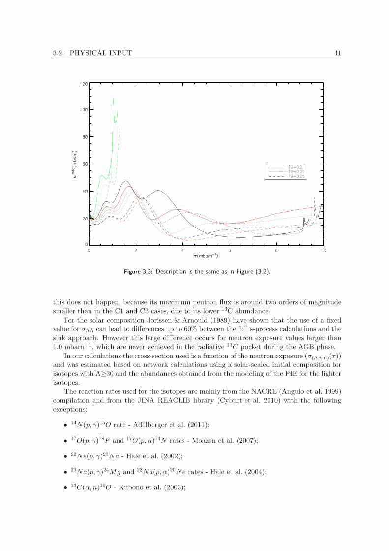
3.2. PHYSICAL INPUT 41
Figure 3.3: Description is the same as in Figure (3.2).
this does not happen, because its maximum neutron flux is around two orders of magnitudesmaller than in the C1 and C3 cases, due to its lower 13C abundance.
For the solar composition Jorissen & Arnould (1989) have shown that the use of a fixedvalue for σAA can lead to differences up to 60% between the full s-process calculations and thesink approach. However this large difference occurs for neutron exposure values larger than1.0 mbarn−1, which are never achieved in the radiative 13C pocket during the AGB phase.
In our calculations the cross-section used is a function of the neutron exposure (σ(AA,n)(τ))and was estimated based on network calculations using a solar-scaled initial composition forisotopes with A≥30 and the abundances obtained from the modeling of the PIE for the lighterisotopes.
The reaction rates used for the isotopes are mainly from the NACRE (Angulo et al. 1999)compilation and from the JINA REACLIB library (Cyburt et al. 2010) with the followingexceptions:
• 14N(p, γ)15O rate - Adelberger et al. (2011);
• 17O(p, γ)18F and 17O(p, α)14N rates - Moazen et al. (2007);
• 22Ne(p, γ)23Na - Hale et al. (2002);
• 23Na(p, γ)24Mg and 23Na(p, α)20Ne rates - Hale et al. (2004);
• 13C(α, n)16O - Kubono et al. (2003);

42 CHAPTER 3. THE EVOLUTIONARY CODE
Figure 3.4: Neutron exposure calculated using the parametrized s-process network in comparison with thesink approach for different values of cross-section: Two cases with fixed cross-section values and one casein which the cross-section was calculated as a function of the neutron exposure. Physical conditions usedin this calculations: T = 108K, ρ = 500 gcm−3. Initial compositions are indicated in the plot. The lineswith labe “0.01” have the same initial composition as C1 except for the 13C mass fraction which is equalto 0.01.
• 22Ne(α, n)25Mg - Jaeger et al. (2001);
• 12C(α, γ)16O - Kunz et al. (2002).
3.2.3 Mass-Loss
One of the main uncertainties in the stellar evolution calculations is the mass-loss. Ob-servations support the idea that negligible mass is lost during the Main Sequence. On theother hand, mass-loss plays an important role in cool giants (RGB and AGB stars): Windsare driven by radiation pressure on the dust grains formed in their cool atmospheres. Severalobservational studies have found a correlation between the mass-loss rate and the pulsationperiod of AGB stars (Schoier & Olofsson 2001; Whitelock et al. 2003; Winters et al. 2003),supporting the idea that mass-loss is enhanced by the pulsation occurring in this evolutionarystage.
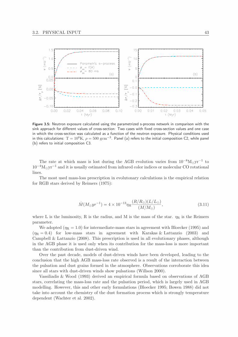
3.2. PHYSICAL INPUT 43
Figure 3.5: Neutron exposure calculated using the parametrized s-process network in comparison with thesink approach for different values of cross-section: Two cases with fixed cross-section values and one casein which the cross-section was calculated as a function of the neutron exposure. Physical conditions usedin this calculations: T = 108K, ρ = 500 gcm−3. Panel (a) refers to the initial composition C2, while panel(b) refers to initial composition C3.
The rate at which mass is lost during the AGB evolution varies from 10−8M⊙yr−1 to
10−4M⊙yr−1 and it is usually estimated from infrared color indices or molecular CO rotational
lines.The most used mass-loss prescription in evolutonary calculations is the empirical relation
for RGB stars derived by Reimers (1975):
M(M⊙yr−1) = 4× 10⁻¹³ηR
(R/R⊙)(L/L⊙)
(M/M⊙), (3.11)
where L is the luminosity, R is the radius, and M is the mass of the star. ηR is the Reimersparameter.
We adopted (ηR = 1.0) for intermediate-mass stars in agreement with Bloecker (1995) and(ηR = 0.4) for low-mass stars in agreement with Karakas & Lattanzio (2003) andCampbell & Lattanzio (2008). This prescription is used in all evolutionary phases, althoughin the AGB phase it is used only when its contribution for the mass-loss is more importantthan the contribution from dust-driven wind.
Over the past decade, models of dust-driven winds have been developed, leading to theconclusion that the high AGB mass-loss rate observed is a result of the interaction betweenthe pulsation and dust grains formed in the atmosphere. Observations corroborate this ideasince all stars with dust-driven winds show pulsations (Willson 2000).
Vassiliadis & Wood (1993) derived an empirical formula based on observations of AGBstars, correlating the mass-loss rate and the pulsation period, which is largely used in AGBmodelling. However, this and other early formulations (Bloecker 1995; Bowen 1988) did nottake into account the chemistry of the dust formation process which is strongly temperaturedependent (Wachter et al. 2002).
44 CHAPTER 3. THE EVOLUTIONARY CODE
Wachter et al. (2002) derived mass-loss rate for solar metallicity using dynamical windmodels for dust-forming carbon-rich atmospheres. This work includes detailed descriptions offormation, growth and evaporation of dust grains. They provide fitting formulae for the mass-loss rate depending on the stellar parameters (Teff ,log(L),M⋆). Mattsson et al. (2010) arguedthat the use of fitting formulae for the mass-loss rates that take into account only the stellarparameters may not be correct. These fitting formulas do not take into account the mass-lossdependence with the amount of condensible carbon (ǫc), for instance. Mattsson et al. (2010)calculations shows an increase in the mass-loss rate by an order of magnitude if ǫc is increasedby a factor of five.
In a more recent study, Wachter et al. (2008) performed mass-loss simulations for lowermetallicities (Z=0.001 and Z=0.01) stars. They have concluded that lower metallicities do notresult in lower mass-loss rates. The average mass-loss rates found in their models are verysimilar to the solar ones. This result was confirmed by Mattsson et al. (2008) simulationsusing an independent wind code. In the light of this, extremelly metal-poor and metal freeAGB stars might have non-negligible mass loss, since their envelope metallicity is increasedup to Z=0.0001 already in the beggining of the TP-AGB phase due to the proton ingestionepisode and continue to increase throughout the TP-AGB evolution.
In our calculations the mass-loss rate derived by (Wachter et al. 2002) is used in stellarevolution code during the TP-AGB phase for stars with pulsation period P > 100 days. Pre-vious AGB calculations using this mass-loss prescription adopted a limiting period of P > 400days (Kitsikis 2008). This cutoff period was used in order to be consistent with the O-richprescription adopted, which is valid only for this regime. In the calculations performed byWeiss & Ferguson (2009) the stars were still in the O-rich regime when the pulsation periodreached 400 days, thus the choice of P=400 days as a critical period also for C-rich regime didnot imply any additional error. In contrast, in the metal-poor regime, due to extra protonmixing, the envelope is quickly enriched with carbon isotopes in the beginning of the TP-AGBphase. The choice of a smaller cutoff period is more consistent with the carbon enrichmentin this case.
The prescription is given as a function of the stellar parameters:
log(M) = −4.52 + 2.47log
(
10−4 L
L⊙
)
− 6.81log
(
Teff
2600K
)
− 1.95log
(
M
M⊙
)
. (3.12)
For the oxygen-rich regime the empirical relation from van Loon et al. (2005) was adopted:
log(M) = −5.65 + 1.05log
(
10−4 L
L⊙
)
− 6.3log
(
Teff
3500K
)
. (3.13)
3.3 Overshooting
Convection is usually described in stellar evolution calculations by the Mixing LengthTheory (MLT). In the MLT, the fluid element loses its identity and mixes with the surround-ings after traveling a certain distance, the mixing length. The mixing length is treated as a
3.3. OVERSHOOTING 45
free parameter in the evolutionary code. In fact, the mixing length parameter αMLT, definedas the ratio between the mixing length and the pressure scale height1, is the adjustable pa-rameter in the code and is calibrated using a solar model. The unstable regions of a star are,then, defined by means of the Schwarzschild criterion: if ∇rad < ∇ad the region is consideredstable. ∇ad is the temperature gradient when the bubble moves adiabatically.
The convective boundary is defined at the point of neutral stability (∇rad = ∇ad), wherethe acceleration of the fluid element is zero. However, at this layer the fluid element has non-zero velocity and, therefore, is able to travel (overshoot) beyond the convective boundary. Acrucial problem rises then: How far is the extension of the mixing beyond the formal convectiveboundaries? The usual approach to answer this question is to introduce a free parameterwhich is a fraction of the pressure scale height, representing the amount of penetration intothe stable regions, and calibrate it using observables affected by the inclusion of overshooting.Schaller et al. (1992) found that in order to reproduce the observed main sequence widthusing instantaneous mixing in the overshooting region a value of dover/Hp = 0.2 should beadopted to the overshooting parameter.
The two-dimensional numerical radiation hydrodynamics simulations performed byFreytag et al. (1996) have shown extra mixing beyond the Schwarzschild borders. Moreover,they found that the velocity declines exponentially at the stable region and that the mixing inthe overshoot region can be described as a diffusive process. In GARSTEC a relation betweenthe diffusion coefficient and the depth of the convective zone was derived.
D = D0e−2zfHp , (3.14)
where z is the distance from the border of the convective zone, Hp is the pressure scale height,D0 is the diffusion coefficient near the edge of the convective zone, and f is a free parameter.
Freytag et al. (1996) found from their simulation a value of f=0.25 for convective envelopesof A-stars and f=1.0 for DA white dwarfs, showing that f strongly depends on the stellarparameters. Herwig et al. (1997) on the other hand, found that an overshooting parameterof f=0.016 reproduces the observed main sequence width. In this same study they found thatthe application of the diffusive overshooting during the AGB results in the occurrence of thethird dredge-up in low-mass stars.
Another important issue regarding overshooting is that it does not have the same efficiencyin all convective borders. For instance, in order to reproduce the solar s-process abundancepatterns Lugaro et al. (2003) have shown that the overshooting parameter value at the bottomof the pulse-driven-convective-zone (PDCZ) should be smaller than the value used at the baseof the convective envelope.
In this thesis diffusive overshooting as described by Freytag et al. (1996) is used in all con-vective boundaries. One single value for the free parameter f is used, unless stated otherwise.When applied, overshooting is considered in all evolutionary phases.
1αMLT = ℓ/Hp

46 CHAPTER 3. THE EVOLUTIONARY CODE

Chapter 4SPNUC: The s-process Code
In this chapter we will give a brief description of the post-processing s-process code.The code solves a nuclear network which contains neutron capture and beta decay reactionsbetween isotopes heavier than 29Si between two stellar models. We have used the s-processnetwork provided by Dr. Aldo Serenelli in the post-processing code.

48 CHAPTER 4. SPNUC: THE S-PROCESS CODE
The calculation of s-process nucleosynthesis coupled to an evolutionary code is quite timeconsuming, since a s-process network contains hundreds of isotopes. A post-processing unit,which uses the thermodynamical output from an evolutionary code as input to solve thenetwork, is then the favored choice when simulating s-process.
Figure 4.1: Schematic diagram of the post-processing code. The code uses the thermodynamical informationfrom two stellar models, separated by ∆t, as input for the network. The network is solved for each gridpoint. The mixing is done after each subtimestep (δt).
The post-processing code uses the model structure (temperature, density, neutron abun-dance, and convection velocity) from evolutionary calculations as input for the s-processcalculations. The calculations are done between two structural models and the evolutionarytimestep between them is divided into smaller burning and mixing steps. All structural quan-tities are kept constant between the two stellar models (Figure 4.2). Within each substep,we first compute changes in chemical composition due to nuclear burning and then mix theconvective (and overshooting) regions.
During the PIE the burning and mixing timescale might be comparable, therefore, theuse of a time-dependent mixing scheme is required. We adopted the time-dependent mixingprescription described in Chieffi et al. (2001).
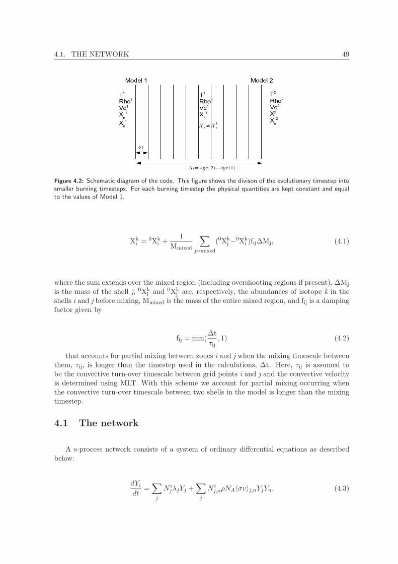
4.1. THE NETWORK 49
Figure 4.2: Schematic diagram of the code. This figure shows the divison of the evolutionary timestep intosmaller burning timesteps. For each burning timestep the physical quantities are kept constant and equalto the values of Model 1.
Xki = 0Xk
i +1
Mmixed
∑
j=mixed
(0Xkj −
0Xki )fij∆Mj, (4.1)
where the sum extends over the mixed region (including overshooting regions if present), ∆Mj
is the mass of the shell j, 0Xki and 0Xk
j are, respectively, the abundances of isotope k in theshells i and j before mixing, Mmixed is the mass of the entire mixed region, and fij is a dampingfactor given by
fij = min(∆t
τij, 1) (4.2)
that accounts for partial mixing between zones i and j when the mixing timescale betweenthem, τij, is longer than the timestep used in the calculations, ∆t. Here, τij is assumed tobe the convective turn-over timescale between grid points i and j and the convective velocityis determined using MLT. With this scheme we account for partial mixing occurring whenthe convective turn-over timescale between two shells in the model is longer than the mixingtimestep.
4.1 The network
A s-process network consists of a system of ordinary differential equations as describedbelow:
dYidt
=∑
j
N ijλjYj +
∑
j
N ij,nρNA〈σv〉j,nYjYn, (4.3)

50 CHAPTER 4. SPNUC: THE S-PROCESS CODE
where Yi is the mole fraction, definied as = Xi/Ai, being Xi the mass fraction and Ai theatomic mass [gmole−1]. The numerical factors are:
N ij = Ni,
N ij,n = Ni/(|Nj |!|Nn|!),
where the numbers, Nm, are positive or negative and specify the number of isotopes mcreated (positive) or destroyed in the reaction.
The categories of thermonuclear reactions involved in equation (4.3) are:1. Decays, photodisintegrations, electron and positron captures (→ λj)2. Two-particle reactions (→ NA〈σv〉j,n) - in our case neutron capture reactionsReactions rates were taken from different sources. The majority of them are used in the
parametrization formula of Thielemann et al. (1987):
r = exp[a0 + a1/T9 + a2(T−1/39 ) + a3(T
1/39 ) + a4T9 + a5(T
5/39 ) + a6lnT9], (4.4)
where T9 = T/109, and ai are the coefficients varying for each reaction.The values for the coefficients ai were taken mainly from the JINA database1 (Cyburt et al.
2010), which uses the most up to date experimental and theoretical cross-sections to derive thecoefficients values, or were calculated by Dr. Aldo Serenelli using the newest measurements ofneutron capture cross-section by the KADONIS 3.0 project (Dillmann et al. 2006). Weak in-teractions rates (electron captures and β decays) were taken mainly from Takahashi & Yokoi(1987) and are interpolated as a function of temperature and electron density. At tempera-tures lower than 106 K we assumed a constant value equal to the laboratory value.
The network used in the code is softwired, making changes in the number of isotopes andreactions used, easy to perform. It was written and kindly provided by Dr. Aldo Serenelli.
Since the neutron fluxes achieved in the calculations presented in this thesis are muchhigher than the “canonical” AGB values (Nn > 1014 cm−3), the isotopes were selected waybeyond the valley of beta stability. In a crude estimate, the timescale for neutron capture isgiven by:
τ =1
Ynρ < σv > Na, (4.5)
where YnρNa is the neutron density, Na is the Avogrado constant, Yn is the neutron numberfraction, and σ is the neutron capture cross-section. For typical temperatures during theAGB phase, a neutron density equal to 1014cm−3 and an average neutron cross-section of< σ >∼ 1000mb, the neutron capture timescale is approximately τ ∼ 3s.
All isotopes with decay lifetimes comparable or longer to the lifetime against neutroncaptures have been included in the network, leading to a network with 580 isotopes and morethan 1000 reactions.
1http://groups.nscl.msu.edu/jina/reaclib/db/

4.2. THE NUMBER OF SUBTIMESTEPS 51
Branching points
If the β decay rate is comparable to the neutron capture one, a branching appears in thes-process. Branching points can also appear when there is a competition between β+ andβ− rates, or when the nucleus decay rate has a strong dependence with temperature and/ordensity, and it can also appear when isomeric states can be produced.
Sometimes the excited state of a nucleus does not de-excite rapidly to the ground state.This excited nucleus is known as isomer and its existence leads to ramifications of the s-process(Ward, Newman & Clayton 1976). Figure (4.3) shows an important s-process branching point,which involves the isomeric state of 85Kr. The probability for the neutron capture onto 84Krto result in the isomeric state of 85Kr is given by the isomeric ratio (IR):
IR =σ(84Kr(n, γ)85Krm)
σtot(84Kr(n, γ)85Kr)= 0.42 (4.6)
Figure 4.3: Krypton branching point is shown. Black boxes indicate stable isotopes, while blue unstableones. Black arrows represent neutron capture reactions while the blue ones represent beta decays.
If the nucleus is non-thermalized the isomeric and the ground states must be treated astwo separate isotopes. Other isomeric states included in our calculations are: 113Cd, 115Cd,114In, 115In, 148Pm, 176Lu, 180Hf , 180Ta.
4.2 The number of subtimesteps
We have performed calculations varying the number of subtimesteps in order to test theabundances dependence with this parameter. As explained before, the code takes the evolu-tionary timestep (∆t) between two subsequent models and divide it into smaller subtimesteps(δt - Figure 4.2). We have chosen two stellar models with different neutron densities (107cm−3
and 1014cm−3), during the PIE of a 1M⊙ star with metallicity Z = 10−8. We did not evolvethe test calculations through the entire PIE evolution, instead, we evolved each stellar modelonly one timestep (∆t) forward.

52 CHAPTER 4. SPNUC: THE S-PROCESS CODE
Figure 4.4: The mass-fraction averaged over the helium convective zone as a function of the number ofsubtimesteps for the isotopes: 30Si and 56Fe. The black line represents the case with Nn = 1014cm−3,while the red line represents the case with Nn = 107cm−3. The blue line indicates the calculations using adiffusive mixing scheme for the case with Nn = 1014cm−3.
Figure 4.5: Same as Figure 4.4 for isotopes: 88Sr and 138Ba.
Figures 4.4 and 4.5 shows the abundance for some selected stable isotopes averaged overthe convective zone. When the neutron density is 107cm−3 the number of subtimesteps usedhas no influence in the final abundances. For neutron densities larger than the canonicalAGB value, the difference between dividing the timestep into two or more subtimesteps can

4.2. THE NUMBER OF SUBTIMESTEPS 53
be larger than one order of magnitude. Different isotopes converge for different number ofsubtimesteps (Figures 4.4 and 4.5). Therefore, we decided to divide the timesteps into 50subtimesteps in order to be closer to the convergence values for most of the isotopes. Wehave also tested a diffusive approach for the mixing scheme (Blue lines in Figures 4.4 and4.5).
Diffusive Mixing
Convection in stars is in general highly turbulent. As discussed in chapter 2 the MLT isthe most used formalism to describe convection in stellar models. Modelling the PIE requiresthe use of a time dependent mixing, since the H-burning timescale is comparable to the mixingtimescale. In the evolutionary code, mixing is treated as a diffusive process. In this case, theequation for composition change can be written as:
dXi
dt=
(
∂Xi
∂t
)
nuc
+∂
∂mr
(
σD∂Xi
∂mr
)
(4.7)
where Xi is the mass-fraction of isotopes i, σ = (4πr2ρ)2 and D = −1/3vlm is the diffusioncoefficient.
We have applied an implicit method to solve the diffusion equation and performed themixing after each burning timestep. Figures 4.4-4.5 shows the abundance dependence with thenumber of subtimesteps for the diffusive approach as well. The difference between using thetime-dependent scheme by Chieffi et al. (2001) and the diffusive approach is very small. Fortwo subtimesteps, the differences can be as large as 20%. However, the differences decreasewith an increasing number of subtimesteps (∼ 1%).

54 CHAPTER 4. SPNUC: THE S-PROCESS CODE

Chapter 5Low-Mass Stars
The bulk of this chapter forms part of an article submitted to Astronomy & Astrophysics.
5.1 Introduction
The peculiar abundance patterns observed in EMP stars are usually attributed to mass-transfer from an AGB companion. AGB stars synthesize carbon and s-process elements,during the thermal-pulses, which are brought up to the surface at each TDU. The discoveryof the proton ingestion episode, however, prompted several attempts to explain the carbon en-richment in such stars by means of internal processes. In this scenario, the observed EMP starwould have undergone PIE during the core He-flash and, then, polluted its own atmospherewith CNO elements in the post-PIE dredge-up. Core He-flash models have shown, however,that the resulting carbon enhancement is usually 1.0-3.0 dex larger than the observed values(Schlattl et al. 2001; Weiss et al. 2004; Picardi et al. 2004). Simulations by Fujimoto et al.(2000) indicated that s-process does not occur during the core He-flash. In these simulations,the timescale of the PIE was too short to make the s-process production viable. Thus, low-mass stars could not be the companion of most carbon enriched EMP stars, since most ofthese stars shows enhancement in s-process elements.
However, recent simulations by Campbell et al. (2010) have shown that PIE during thecore He-flash results in a large neutron production and, therefore, in a large s-process pro-duction. A recent observational discovery also strengthened the necessity of understandingthe evolution of EMP low-mass stars. A star with metallicity [Fe/H] = −4.89 and no en-hancement in CNO elements was found in the Galactic halo (Caffau et al. 2011, 2012). Thisiron abundance corresponds to a total metallicity of Z ≤ 7.40× 10⁻⁷, which makes SDSSJ102915+172927, the star with the lowest metallicity ever detected. The two hyper metal-poor stars ([Fe/H] < −5.0) found in the past decade are in fact more metal rich than SDSSJ102915+17292 (Z ∼ 10−4), since they present high levels of carbon, nitrogen, and oxygenenhancement. The extremely low metallicity found for SDSS J102915+172927 puts intoquestion the claims of a minimum metallicity required for the formation of low-mass stars(Bromm & Loeb 2003; Schneider et al. 2003).
Up to now, simulations of s-process during the PIE are limited to one mass and onemetallicity (M = 1.0M⊙/Z = 10−8 - Campbell et al. (2010)). Fujimoto et al. (2000) did not
56 CHAPTER 5. LOW-MASS STARS
perform actual s-process calculations. In reality, they suggested the absence of s-processduring the core He-flash PIE based on the short duration of this phenomenon in their models.It is important, then, to understand the nucleosynthesis during the PIE which might be animportant source of s-process production during the early stages of the Galaxy. In order todo this, we have performed evolutionary and post-processing s-process calculations of low-mass stars with metallicities (Z ≤ 10−7) and explored the model uncertainties (especiallyconvection) and their impact in the s-process.
5.2 The Models
We performed evolutionary calculations of 1 M⊙ stellar models from the zero-age main se-quence to the dredge-up after the PIE. The composition is solar-scaled with metallicitiesZ = 0, Z = 10−8, and Z = 10−7. Our “standard” models (M1, M2, M6, and M7 - see Table5.1) do not included overshooting or metal diffusion. In order to check the s-process depen-dence with stellar mass, we computed an additional model with metallicity Z = 10−8 andmass M = 0.82M⊙ (M6 in Table 5.1). Due to convergence problems, it was not possible tocontinue the simulation beyond the H-flash for model M5.
Mixing in convective regions is modeled as a diffusive process. The diffusion coefficient inconvective regions is taken as Dc = 1/3v × ℓ, where v is the convective velocity derived fromMLT and ℓ is the mixing length. It has been suggested that during the PIE, the reactivenature of the hydrogen material adds some buoyancy to the sinking elements and this resultsin a reduced efficiency of the mixing (Herwig et al. 2011). We have mimicked this situationby using a reduced diffusion coefficient by dividing the above relation by 10 in a model withZ = 10−8 (model M3 - Table 5.1).
Finaly, we have also computed additional models with metallicity Z = 10−8 including over-shooting. Overshooting has been modeled as an exponentially decaying diffusive coefficient, asdescribed in Freytag et al. (1996), and has been included in all convective boundaries. In or-der to test the influence and associated uncertainties of this poorly-understood phenomenon,two values of the free parameter f that determines the extension of the overshooting regionshave been chosen: f = 0.016 and 0.07 (models M4 and M5 respectively - Table 5.1). The firstvalue is a standard choice for this prescription of overshooting because it gives comparableresults in the main sequence as the canonical choice of 0.2 pressure scale heights (Magic et al.2010), a value known to reproduce different observational constraints such as the the widthof the main sequence observed in different open clusters. The higher value is intended torepresent a case where overshooting is much larger than in convective cores and deep stellarenvelopes, and closer to what was originally found by Freytag et al. (1996) for thin convectiveenvelopes of A-type stars. Incidentally, this amount of overshooting gives the right lithiumdepletion in solar models (Weiss et al. 2000).

5.3. FROM THE ZAMS TO THE PIE 57
Model Mass (M⊙) Metallicity (Z)
M1 1.0 zero —M2 1.0 10−8 —M3 1.0 10−8 R.M.EM4 1.0 10−8 OV.M5 1.0 10−8 OV.M6 0.82 10−8 —M7 1.0 10−7 —
Table 5.1: List of low-mass stars models. R.M.E stands for Reduced Mixing Efficiency and OV stands forovershooting. A detailed description of the models is found in the text.
5.3 From the ZAMS to the PIE
The main sequence evolution of EMP and zero metallicity stars does not differ significantlyfrom the evolution of their metal-rich counterparts, since the H-burning in the core is dom-inated by the pp chain in all cases. Figure 5.1 shows the HRD for the computed models.There is no difference in the morphology of the HRD up to the tip of the RGB for the modelswith mass 1.0M⊙ and metallicity 10−8 ≤ Z ≤ 10−7. The model with metallicity Z=0 showsa loop at the SGB, not observed in other models (point A in Figure 5.1). This loop resultsfrom a thermal runaway happening due to the increase importance of the CNO cycle in theH-burning. Just before H is exhausted in the center, the core contracts, increasing its temper-ature and density. The increase in temperature and density in the core, results in an increasein the efficiency of the 3α reactions and, therefore, in the production of 12C. The energyreleased by the CNO cycle strongly increases, due to the increase in 12C abundance, and aflash occurs. This flash produces the loop in the HRD.
In Table 5.2 we present the stellar lifetimes of various evolutionary stages correspondingto the tracks of Figure 5.1. We compare our results mainly to the results by Campbell (2007)which calculated a grid of models with metallicities [Fe/H] ≤ −3.0 and masses 0.85 ≤ M ≤ 3.0.Zero metallicity models will also be compared to (Marigo et al. 2001; Siess et al. 2002), whopublished an extensive grid of models for this metallicity. We have defined the MS lifetimeas the time between the ZAMS and the turn-off. For the zero metallicity model (M1), wehave found MS lifetimes 8% and 11% smaller than the values given by Marigo et al. (2001)and Siess et al. (2002), respectively. These differences could be the result of a larger initialhydrogen content used in these studies (X=0.77,Y=0.23). In comparison to Campbell (2007)results, which used the same initial H abundance (X=0.755,Y=0.245), the MS lifetime ofmodel M1 is only 3% smaller than the value provided. Our standard models M2 and M7are in good agreement with similar models ([Fe/H] = −6.5 and [Fe/H] = −5.45) simulated byCampbell (2007), showing differences smaller than 7%. The MS lifetime slightly decreaseswith increasing metallicity, which is probably due to a larger contribution of the CNO cycleto the H-burning.
Lifetime values for the subgiant branch and the red giant branch phases are providedonly by Campbell (2007). The SGB lifetime is defined as the time bewteen the turn-off andthe base of the RGB. Our models have SGB lifetimes usually 20% smaller than models byCampbell (2007), except for M1 which has slightly larger lifetime and M7 which is about 30%shorter.
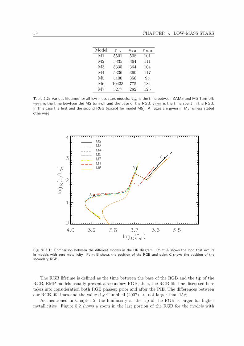
58 CHAPTER 5. LOW-MASS STARS
Model τms τSGB τRGB
M1 5501 508 101M2 5335 364 111M3 5335 364 104M4 5336 360 117M5 5400 356 95M6 10433 775 184M7 5277 282 125
Table 5.2: Various lifetimes for all low-mass stars models. τms is the time between ZAMS and MS Turn-off.τSGB is the time bewteen the MS turn-off and the base of the RGB. τRGB is the time spent in the RGB.In this case the first and the second RGB (except for model M5). All ages are given in Myr unless statedotherwise.
Figure 5.1: Comparison between the different models in the HR diagram. Point A shows the loop that occursin models with zero metallicity. Point B shows the position of the RGB and point C shows the position of thesecondary RGB.
The RGB lifetime is defined as the time between the base of the RGB and the tip of theRGB. EMP models usually present a secondary RGB, then, the RGB lifetime discussed heretakes into consideration both RGB phases: prior and after the PIE. The differences betweenour RGB lifetimes and the values by Campbell (2007) are not larger than 15%.
As mentioned in Chapter 2, the luminosity at the tip of the RGB is larger for highermetallicities. Figure 5.2 shows a zoom in the last portion of the RGB for the models with
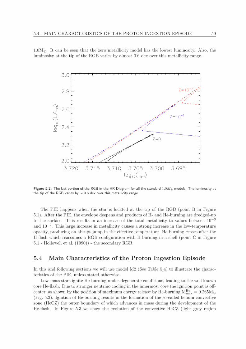
5.4. MAIN CHARACTERISTICS OF THE PROTON INGESTION EPISODE 59
1.0M⊙. It can be seen that the zero metallicity model has the lowest luminosity. Also, theluminosity at the tip of the RGB varies by almost 0.6 dex over this metallicity range.
Figure 5.2: The last portion of the RGB in the HR Diagram for all the standard 1.0M⊙ models. The luminosity atthe tip of the RGB varies by ∼ 0.6 dex over this metallicity range.
The PIE happens when the star is located at the tip of the RGB (point B in Figure5.1). After the PIE, the envelope deepens and products of H- and He-burning are dredged-upto the surface. This results in an increase of the total metallicity to values between 10−3
and 10−2. This large increase in metallicity causes a strong increase in the low-temperatureopacity, producing an abrupt jump in the effective temperature. He-burning ceases after theH-flash which reassumes a RGB configuration with H-burning in a shell (point C in Figure5.1 - Hollowell et al. (1990)) - the secondary RGB.
5.4 Main Characteristics of the Proton Ingestion Episode
In this and following sections we will use model M2 (See Table 5.4) to illustrate the charac-teristics of the PIE, unless stated otherwise.
Low-mass stars ignite He-burning under degenerate conditions, leading to the well knowncore He-flash. Due to stronger neutrino cooling in the innermost core the ignition point is off-center, as shown by the position of maximum energy release by He-burning MHe
max = 0.265M⊙
(Fig. 5.3). Ignition of He-burning results in the formation of the so-called helium convectivezone (HeCZ) the outer boundary of which advances in mass during the development of theHe-flash. In Figure 5.3 we show the evolution of the convective HeCZ (light grey region

60 CHAPTER 5. LOW-MASS STARS
extending from Mr/M⊙ = 0.265 up to 0.535) during the time following the maximum helium-burning luminosity up the the moment where the PIE starts. The combination of an off-centerHe-burning ignition and a low entropy barrier between the He- and H-burning shells in thevery metal-poor environment allows the HeCZ to reach hydrogen-rich layers (Hollowell et al.1990) and giving rise to the PIE.
The HeCZ reaches the radiatively stratified H-rich layers on top (initially representedby white region above Mr/M⊙ = 0.535) soon after the He-burning luminosity reaches itsmaximum value. Protons are then mixed down into the HeCZ and are captured by theabundant 12C, creating 13C. The H-burning luminosity increases while the HeCZ continuesexpanding (in mass). Note that the penetration of the HeCZ into the H-rich region occurs in anarrow region of only a few parts per thousand of solar masses and it is barely visible around0.535 M⊙ in Figure 5.3. Around 0.23 years after the He-luminosity reached its maximuma secondary flash happens, the H-flash, with a H-burning luminosity comparable or largerthan the He-burning luminosity (log10(L
Hemax/L⊙) = 10.67, log10(L
Hmax/L⊙) = 10.73). The
burning timescale for hydrogen through the 12C(p, γ) reaction becomes shorter as protonstravel downwards in the HeCZ until a point inside the HeCZ is reached where the burningand mixing timescales are comparable. At this position (MH
max = 0.29M⊙) the energy releasedby H-burning is maximum and temperature rises quickly, resulting in an inversion in thetemperature profile that eventually leads to the splitting of the convective zone. This preventsthe penetration of protons further down into the He-CZ.
The splitting results in two convective zones: a small HeCZ and an upper convective zonewhich is referred to as hydrogen convective zone (HCZ). The outer boundary of the HCZcontinues to advance in mass. In about 700 years, the envelope deepens and products ofburning during and after the PIE are dredged-up to the surface. The envelope is enrichedmainly in C, N, and O. Similarly to results by other authors, the amount of C and N brought upto the surface is too large compared to the abundances observed in EMP stars (values in Table5.7 are more than 3 dex larger than the average CEMP’s carbon abundance). Enrichment ins-process depends strongly on the nucleosynthesis before the splitting of the HeCZ and willbe discussed in the following section. The long-term evolution before and after the PIE isillustrated in Figure 5.4, where time has been set to zero at the moment when LHe reachesits maximum.
The time between maximum He-burning luminosity and the onset of hydrogen mix-ing (∆tmix) in our calculations is usually larger than the interval found in other studies(Hollowell et al. 1990; Suda et al. 2007; Picardi et al. 2004). This might partially be the re-sult of the larger mass between the bottom of the HeCZ and the location of the base of theH-rich layer in our models. Our predicted ∆tmix varies from 10−2 to 1 year (depending on themetallicity and the convection efficiency assumed in the models), while in other studies thisvalue ranges from 10−3 to 10−2 years. The main properties of the core helium flash and thePIE are summarized in Table 5.4. In can be seen in Table 5.4 that, for a given stellar mass,the larger the mass between the He-flash ignition point and the H-shell (∆Mig) the higher is∆tmix.
Table 5.3 shows a summary of the literature theoretical studies of low-mass stars. Ourvalues of ∆Mig are usually larger than the values found in the literature, with the exception ofthe models by (Schlattl et al. 2001, 2002) that used a slightly different version of GARSTEC.The maximum ∆Mig reported by other groups in the literature for which PIE happens is0.24. On the other hand, our models present ∆Mig only larger than this value. Suda et al.(2007) suggested that the inner He-flash ignition point obtained by Schlattl et al. (2001),

5.4. MAIN CHARACTERISTICS OF THE PROTON INGESTION EPISODE 61
Figure 5.3: Upper Panel: Time evolution of convective zones (grey areas) in our model M2 during the PIE. Thicksolid and dot-dashed lines represent the position of maximum energy release due to H-burning and He-burning,respectively. The splitting of the HeCZ around t− t0 = 0.225 yr is evident with the formation of a detached HCZ(dark grey area). Bottom Panel: Evolution of H-burning (solid line) and He-burning (dashed line) luminosities.t = t0 corresponds to the time of maximum He-burning luminosity.
and also observed in our models, might have two sources: the neutrino bremsstrahlung,not included in the fitting formula for neutrino energy-loss rates given by Munakata et al.(1985) and the equation of state. Suda et al. (2007) performed an evolutionary model usingthe fitting formula by Munakata et al. (1985) in order to check if the absence of neutrinobremsstrahlung would cause the inward shift of the ignition point. They found a ignition pointonly 10% smaller than the models including neutrino bremsstrahlung. This 10% reductionis, however, too small to account for the inner position found by Schlattl et al. (2001). Wehave performed an evolutionary calculation using Irwin’s EOS (Cassisi et al. 2003) for thezero metallicity case: the ignition point is only 3% larger than found in M1.
An interesting diagnostic is the distance, in mass, that protons are mixed down beforethe splitting of the HeCZ occurs (∆Mc - Campbell 2007). It appears that, for a given mass,this quantity is an indicator of the amount of pollution that occurs after the PIE (Campbell2007). Table 5.4 shows that the larger ∆Mc, the larger is the abundance of CNO elements inthe surface, with the exception of model M4.
An important property of the PIE for the s-process is the time between the onset ofhydrogen mixing and the splitting of the convective zone, here referred to as ∆tPIE. After thesplitting of the HeCZ, the abundance of 14N, the main neutron poison in this environment,in the HCZ rapidly builds up. As the 13C to 14N ratio drops below unity neutrons arepredominantly captured by 14N(n, p)14C and the s- process is effectively shut down. Therefore,∆tPIE determines the timescale for s-processing. In our calculations ∆tPIE is in the range∼0.1 to 1 yr (Table 5.4), about an order of magnitude larger than in some other studies

62 CHAPTER 5. LOW-MASS STARS
Authors M∗ Z MHemax Mc ∆Mig
Fujimoto et al. 1990 0.77 zero 0.41 0.53 0.12Schlattl et al. 2001 1.00 zero 0.15 0.48 0.33Schlattl et al. 2002 0.82 zero 0.31 0.61 0.30Siess et al. 2002 1.00 zero 0.31 0.49 0.18Picardi et al. 2004 0.80 zero 0.35 0.52 0.17
0.80 10−8 0.38 0.54 0.160.80 10−7 0.35 0.55 0.201.00 zero 0.26 0.50 0.24
Campbell 2007 0.85 ∼ 10−7 0.30 0.53 0.230.85 ∼ 10−8 0.33 0.52 0.190.85 zero 0.28 0.49 0.211.00 ∼ 10−8 0.31 0.52 0.211.00 zero 0.25 0.49 0.23
Suda et al. 2007 0.80 zero 0.36 0.51 0.151.00 zero 0.33 0.50 0.17
Suda & Fujimoto 2010 0.80 ∼ 10−7 — 0.54 —0.80 zero — 0.51 —1.00 ∼ 10−7 — 0.53 —1.00 zero — 0.50 —
Table 5.3: A summary of the literature for theoretical studies of low-mass stars of extremelly low and zerometallicity. All masses are given in solar mass unit.
(e.g. Hollowell et al. (1990)). In contrast, Campbell et al. (2010) presented a model withmetallicity [Fe/H] = −6.5 in which ∆tPIE ∼ 20 yrs, about two orders of magnitude larger thanour findings. The large differences in ∆tPIE may be at the core of the seemingly contradictoryresults regarding the production of s-process elements during the core He-flash found bydifferent authors.
We note here that splitting of the He-CZ is ubiquitous in all 1-dimensional simula-tions of the PIE during the core helium flash (Hollowell et al. 1990; Schlattl et al. 2001;Campbell & Lattanzio 2008). Splitting of the HeCZ (shell) is also found in PIE resultingfrom very late thermal pulses in post-AGB stars (Herwig 2001; Althaus et al. 2005) as wellas in simulations of the early phases of the TP-AGB in very metal-poor stars (Fujimoto et al.2000; Serenelli 2006; Cristallo et al. 2009a). On the other hand, recent hydrodynamic 3-dimensional simulations of the TP-AGB phase for a low-mass star (Stancliffe et al. 2011)have not shown splitting of the HeCZ, although the authors argued this might be an artifactof the low resolution used in the calculations.

5.4. MAIN CHARACTERISTICS OF THE PROTON INGESTION EPISODE 63
Figure 5.4: Long-term evolution of the 1 M⊙, Z=10−8 stellar model during the development of the core He-flash,the PIE, and the subsequent dredge-up event. t = t0 corresponds to the time of maximum He-burning luminosity.As in Figure 5.3, thick solid and dot-dashed lines represent the position of maximum energy release due to H-burningand He-burning, respectively. Merging of the HCZ and the stellar envelope occurs around 770 yr after the PIE takesplace.

64 CHAPTER 5. LOW-MASS STARS
Model LHemax LH
max MHemax MHe
c ∆tmix ∆tPIE MHmax ∆Mc ∆Mig ZCNO
M1 9.972 10.48 0.175 0.488 1.400 1.356 0.290 0.198 0.313 0.010M2 10.67 10.73 0.265 0.535 0.024 0.202 0.288 0.247 0.270 0.018M3 10.67 9.828 0.265 0.535 0.028 0.234 0.333 0.202 0.270 0.017M4 10.68 10.87 0.263 0.536 0.019 0.104 0.281 0.255 0.273 0.015M5 10.68 11.17 0.261 0.534 6.5× 10⁻³ 0.041 0.267 0.267 0.273 —M6 10.68 11.05 0.277 0.562 0.002 0.075 0.298 0.264 0.285 0.025M7 11.10 10.37 0.289 0.572 0.200 2.204 0.293 0.279 0.283 0.023
Table 5.4: Main properties of the proton ingestion episode. LHemax and LH
max are the logarithm of themaximum He-burning luminosity and the maximum H-burning luminosity in units of solar luminosity, re-spectively. MHe
max is the position of maximum energy released by He-burning. MHec is the core mass. ∆tmix
is the time between maximum He-burning luminosity and the onset of hydrogen mixing in years. ∆tPIE
is the time between maximum He-burning luminosity and the splitting of the convective zone in years.M4 and M5 are the models including overshooting with overshooting parameters f=0.016 and f=0.07,respectively.MH
max is the position of maximum energy release by H-burning. ∆Mc is the distance, in mass,that the H-shell moves inwards during the PIE (M⊙). ∆Mig is the distance, in mass, between the He-flashignition point and the H-shell (M⊙). All masses are given in units of solar mass. ZCNO is the surfacemass-fraction of CNO elements.
5.5 Neutron Production and the s-process
During the PIE, 13C is formed by proton captures on 12C and mixed throughout the entireHeCZ. The abundance of 13C in the convective zone increases by several orders of magnitudeduring ∆tPIE (from X13C ∼ 10−10 to X13C ∼ 10−3 in mass-fraction).
Neutrons are produced by the reaction 13C(α, n)16O, near the bottom of the convectivezone, reaching maximum neutron density values larger than 1014cm−3. 12C is the most abun-dant isotope, besides 4He, in the HeCZ and thus neutrons are mainly captured by it and enterinto the recycling reaction 12C(n, γ)13C(α, n)16O. At the beginning of the proton ingestion,13C is much less abundant than 14N, and neutrons not captured by 12C are captured by 14N.As the PIE progresses, the 13C abundance increases and so does the 13C/14N abundanceratio and the neutron density (Fig. 5.5 and Fig. 5.6). Eventually, 13C/14N abundance ratiogets larger than unity and more neutrons are free to be captured by heavy elements. The13C/14N abundance ratio reaches a maximum value around ∆t ∼ 0.10 yrs after the PIE starts.Hydrogen abundance is now large enough to enhance the competition between 13C(p, γ)14Nand 13C(α, n)16O. Thus, the 13C/14N abundance ratio starts to decrease, leading to a shal-lower increase in neutron density than before. After the splitting, the bottom of the HeCZmoves slightly outwards and cools down and the supply of fresh protons into the HeCZ stops,consequently the neutron flux is quickly suppressed (Fig. 5.5).
Regarding the production of s-process elements in a given environment (which determines,among others, the number of seed nuclei present), the key quantity is the time-integratedneutron flux, or neutron exposure, given by
τ =
∫ tf
tivTnndt (5.1)
where vT is the thermal velocity of neutrons, ti is the beginning of the neutron flux, tf is theend of the neutron flux, and nn their number density. In the case of the PIE, the other relevant

5.5. NEUTRON PRODUCTION AND THE S-PROCESS 65
Figure 5.5: Upper Panel: Time evolution of maximum neutron density in our Z = 10−8 model (M2) at M=0.265M⊙. Bottom Panel: Evolution of the temperature near the bottom of the HeCZ. In both cases the sudden changeat t− t0 ≈ 0.225 yr reflects the splitting of the HeCZ.
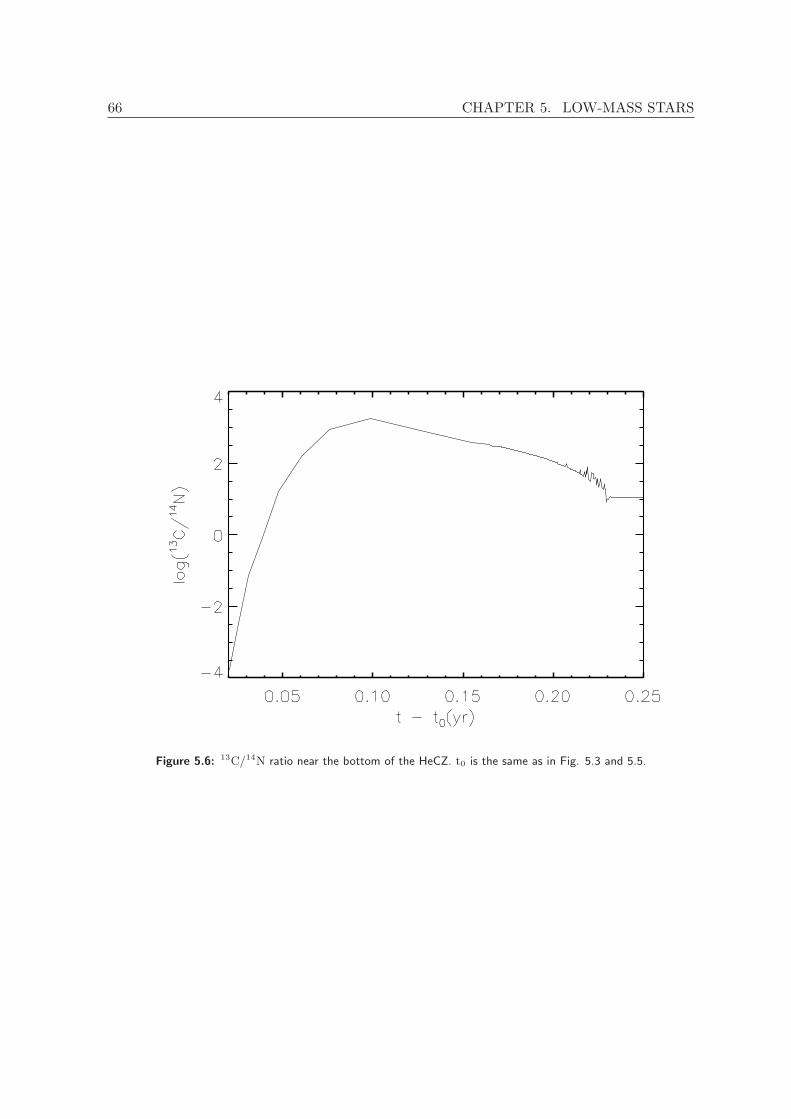
66 CHAPTER 5. LOW-MASS STARS
Figure 5.6: 13C/14N ratio near the bottom of the HeCZ. t0 is the same as in Fig. 5.3 and 5.5.

5.5. NEUTRON PRODUCTION AND THE S-PROCESS 67
Figure 5.7: Time evolution of neutron exposure. Solid lines represent the neutron exposure at the position ofmaximum neutron density (i.e. near the bottom of the HeCZ) and dashed lines represent the average neutronexposure in the convective zone. Blue line: model including overshooting (f=0.016 - M4), red line: standardZ = 10−8 model (M2), black line: reduced convection efficiency (M3), and green line: model including overshooting(f=0.07).
quantity is the splitting timescale ∆tPIE which, as we discuss below, determines the timespanover which neutrons are effectively produced and is therefore the cutoff to the integration inEquation 5.1.
In Figure 5.7 we show, in solid lines, the neutron exposure as a function of time nearthe bottom of the HeCZ, where the maximum neutron flux is achieved. Results for thereference model, M2, are depicted in red. In the same figure, dashed lines denote the neutronexposure averaged across the entire convective zone. For comparison, typical values for theneutron exposure during the AGB phase are roughly two orders of magnitude smaller thanthe maximum neutron exposure at the bottom of the HeCZ.
At the beginning of the PIE iron-peak elements (mainly 56Fe) are converted to elementsof the first s-process peak (Sr, Y, Zr). The 56Fe abundance is strongly reduced, reaching itsminimum value at about 0.17 yrs after the maximum helium-burning luminosity. Between0.17 and 0.22 yrs after the He-flash, strontium is converted into barium and, subsequently intolead. The mass fraction of Fe, Sr, Ba, and Pb in the convective zone are shown in Figure 5.8.Near the end of the PIE, as the outer boundary of the HCZ advances, freshly dredged-downiron increases the 56Fe abundance by an order of magnitude.
After the splitting of the HeCZ, the upper convective zone, HCZ, penetrates further intothe H-rich layers above and 12C is converted into 14N. The cooling of the HCZ effectively

68 CHAPTER 5. LOW-MASS STARS
switches off α-captures by 13C, and 14N captures most of the remaining neutrons available,effectively quenching s-processing. Therefore, the abundances of heavy elements in the HCZremain unchanged by nuclear burning after the splitting. They do not change until the HCZmerges with the stellar envelope and the processed material is dredged-up to the surface.
5.5.1 The influence of convective mixing
The treatment of convection and the associated mixing in stellar evolution calculations issubject to fundamental uncertainties that can not be properly addressed in 1D models. Nev-ertheless, we can try to understand how varying the mixing efficiency in convective regions orthe extent of the mixing regions (e.g. by including overshooting) affect the basic propertiesof the PIE. In turn, this will affect neutron production and the ensuing creation of s-processelements.
Let us first discuss models including overshooting. Model M4 is computed by using amoderate amount of overshooting characterized by f = 0.016 (Sect. 5.2). The extendedconvective boundary in this model allows a larger penetration of the HeCZ into H-rich layers.More fuel is ingested into the HeCZ and thus a faster, but shorter, evolution of the protoningestion episode is achieved. In Figure 5.7 solid lines represent the time evolution of theneutron exposure at the location of maximum neutron density. Comparison of models M2 andM4 (red and blue lines respectively) show that the more vigorous entrainment of hydrogen intothe HeCZ in model M4 produces an early and steeper increase in the neutron exposure. Also,the maximum neutron flux is almost a factor of two larger in model M4 than in model M2.However, the faster release of nuclear energy by hydrogen burning leads to the PIE lasting lessthan half the time it does in the case of no overshooting. This leads to a significantly smallerfinal neutron exposure in the case of M4 as seen in Figure 5.7. To confirm this trend, we havecomputed an additional model with a large overshooting parameter f = 0.07. For this model,results shown in green in Figure 5.7 confirm that a larger overshooting region leads to a moreviolent hydrogen ingestion (as seen by the quick and steep rise in neutron production) but ofshorter duration and, overall, reduced efficiency in the final neutron exposure. Quantitatively,the difference between the final neutron exposure for the two models with overshooting is nottoo large, despite the ∼ 50% difference in ∆tPIE (see blue and gree solid lines in Figure 5.7).
As mentioned before, we have found shorter splitting timescales than other recent cal-culations (e.g. those of Campbell et al. (2010)). In order to mimic these longer splittingtimescales, we computed a model with a reduced convective mixing efficiency. In our calcula-tions we have simply achieved this by dividing the diffusion coefficient by a constant factor.In model M3 this reduction is by one order of magnitude. As expected, a reduced mixingefficiency results in a larger ∆tPIE, although the difference is not too significant compared tothe standard case (see Models M2 and M3 in Table 5.4). This increase in time, however, isenough to produce a total neutron exposure at maximum (black solid line) about 50% largerthan in the standard case; this should favor the production of the heaviest s-process isotopes.In terms of structure properties, while the inclusion of overshooting moves the splitting posi-tion inwards, the reduced mixing efficiency moves this position outwards (MH
max in Table 5.4).This slightly reduces the amount of CNO elements dredged-up.
In a radiative environment, the neutron exposure at the position of maximum neutrondensity would result in a strong enhancement in Pb, due to the repeated neutron capturesin a static environment, in all cases. However, in a convective environment, the interplaybetween burning and convection is important. The mixing timescale is shorter than the

5.5. NEUTRON PRODUCTION AND THE S-PROCESS 69
Figure 5.8: Evolution of the mass fraction of isotopes representative of the three s-process abundance peaks and56Fe as a function of time. These abundances were sampled at the position 0.4 M⊙. They are representative ofthe entire convective zone and, after the splitting, are located in the HCZ which later comes into contact with thestellar envelope.

70 CHAPTER 5. LOW-MASS STARS
overall phase of s-process production and, thus, the relevant quantity for the final productionis the averaged neutron exposure. Figure 5.7 shows the neutron exposure averaged over theconvectively mixed zone (dashed lines). As it can be seen, the averaged neutron exposure isstrongly reduced in the overshooting model (blue dashed line), but it is not much affected bythe reduction in the mixing efficiency (black dashed line). This leads to small differences inthe final production of s-process elements despite the 50% difference in the neutron exposureat the bottom of the HeCZ. Figure 5.9 shows the abundance distribution inside the HeCZright before the splitting. As discussed above, the smaller neutron exposure of model M4favors the production of elements from the first and second s-process peak and produces lessPb than models M2 and M3.
Figure 5.9: Abundance distribution inside the HeCZ right before the splitting.
5.5.2 The absence of iron-peak seeds: zero metallicity case
Goriely & Siess (2001) have studied the occurrence of s-process nucleosynthesis during theAGB phase of a 3M⊙ stellar model with initial zero metallicity. They found that, byparametrizing the formation of the 13C-pocket during the third dredge-up, neutron densi-ties of the order of 109cm−3 can be reached. Furthermore, their results showed this is highenough for an efficient production of s-process elements to occur starting from lighter seeds(C-Ne), even in the complete absence of iron-peak elements.
The calculations of the 1 M⊙ metal-free model presented in this thesis (model M1), showthat low-mass stars can also produce light elements that might act as seeds of s-processnucleosynthesis. This occurs in two steps. First, during the transition from the subgiantto the red giant phase, the interior temperature is high enough to start helium-burning andproduce carbon. Once the carbon mass-fraction is Xc ∼ 10−11, the CNO cycle is ignited and asmall thermal runaway occurs due to the sudden increase in the efficiency of the CNO burning
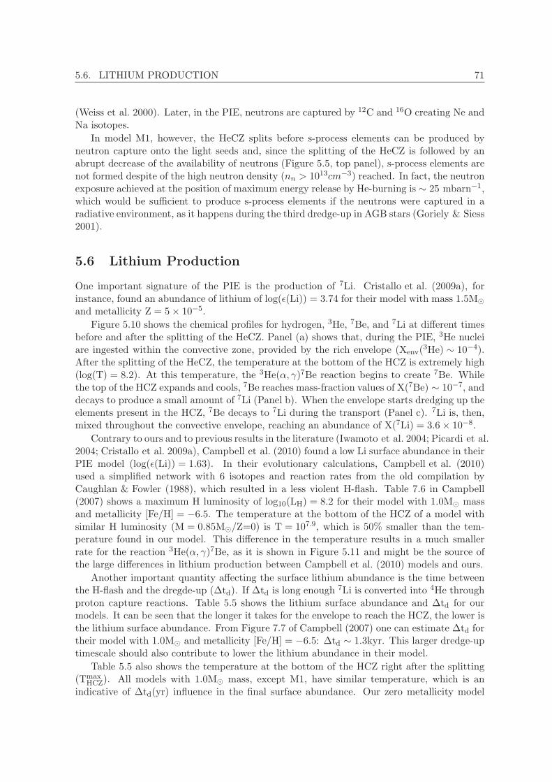
5.6. LITHIUM PRODUCTION 71
(Weiss et al. 2000). Later, in the PIE, neutrons are captured by 12C and 16O creating Ne andNa isotopes.
In model M1, however, the HeCZ splits before s-process elements can be produced byneutron capture onto the light seeds and, since the splitting of the HeCZ is followed by anabrupt decrease of the availability of neutrons (Figure 5.5, top panel), s-process elements arenot formed despite of the high neutron density (nn > 1013cm−3) reached. In fact, the neutronexposure achieved at the position of maximum energy release by He-burning is ∼ 25 mbarn−1,which would be sufficient to produce s-process elements if the neutrons were captured in aradiative environment, as it happens during the third dredge-up in AGB stars (Goriely & Siess2001).
5.6 Lithium Production
One important signature of the PIE is the production of 7Li. Cristallo et al. (2009a), forinstance, found an abundance of lithium of log(ǫ(Li)) = 3.74 for their model with mass 1.5M⊙
and metallicity Z = 5× 10⁻⁵.
Figure 5.10 shows the chemical profiles for hydrogen, 3He, 7Be, and 7Li at different timesbefore and after the splitting of the HeCZ. Panel (a) shows that, during the PIE, 3He nucleiare ingested within the convective zone, provided by the rich envelope (Xenv(
3He) ∼ 10−4).After the splitting of the HeCZ, the temperature at the bottom of the HCZ is extremely high(log(T) = 8.2). At this temperature, the 3He(α, γ)7Be reaction begins to create 7Be. Whilethe top of the HCZ expands and cools, 7Be reaches mass-fraction values of X(7Be) ∼ 10−7, anddecays to produce a small amount of 7Li (Panel b). When the envelope starts dredging up theelements present in the HCZ, 7Be decays to 7Li during the transport (Panel c). 7Li is, then,mixed throughout the convective envelope, reaching an abundance of X(7Li) = 3.6× 10⁻⁸.
Contrary to ours and to previous results in the literature (Iwamoto et al. 2004; Picardi et al.2004; Cristallo et al. 2009a), Campbell et al. (2010) found a low Li surface abundance in theirPIE model (log(ǫ(Li)) = 1.63). In their evolutionary calculations, Campbell et al. (2010)used a simplified network with 6 isotopes and reaction rates from the old compilation byCaughlan & Fowler (1988), which resulted in a less violent H-flash. Table 7.6 in Campbell(2007) shows a maximum H luminosity of log10(LH) = 8.2 for their model with 1.0M⊙ massand metallicity [Fe/H] = −6.5. The temperature at the bottom of the HCZ of a model withsimilar H luminosity (M = 0.85M⊙/Z=0) is T = 107.9, which is 50% smaller than the tem-perature found in our model. This difference in the temperature results in a much smallerrate for the reaction 3He(α, γ)7Be, as it is shown in Figure 5.11 and might be the source ofthe large differences in lithium production between Campbell et al. (2010) models and ours.
Another important quantity affecting the surface lithium abundance is the time betweenthe H-flash and the dregde-up (∆td). If ∆td is long enough 7Li is converted into 4He throughproton capture reactions. Table 5.5 shows the lithium surface abundance and ∆td for ourmodels. It can be seen that the longer it takes for the envelope to reach the HCZ, the lower isthe lithium surface abundance. From Figure 7.7 of Campbell (2007) one can estimate ∆td fortheir model with 1.0M⊙ and metallicity [Fe/H] = −6.5: ∆td ∼ 1.3kyr. This larger dredge-uptimescale should also contribute to lower the lithium abundance in their model.
Table 5.5 also shows the temperature at the bottom of the HCZ right after the splitting(Tmax
HCZ). All models with 1.0M⊙ mass, except M1, have similar temperature, which is anindicative of ∆td(yr) influence in the final surface abundance. Our zero metallicity model
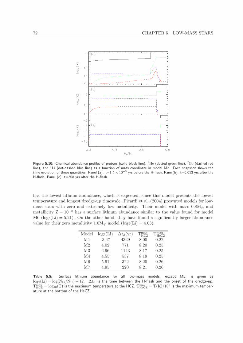
72 CHAPTER 5. LOW-MASS STARS
Figure 5.10: Chemical abundance profiles of protons (solid black line), 3He (dotted green line), 7Be (dashed redline), and 7Li (dot-dashed blue line) as a function of mass coordinate in model M2. Each snapshot shows thetime evolution of these quantities. Panel (a): t=1.5× 10⁻³ yrs before the H-flash, Panel(b): t=0.013 yrs after theH-flash. Panel (c): t=308 yrs after the H-flash.
has the lowest lithium abundance, which is expected, since this model presents the lowesttemperature and longest dredge-up timescale. Picardi et al. (2004) presented models for low-mass stars with zero and extremely low metallicity. Their model with mass 0.8M⊙ andmetallicity Z = 10−8 has a surface lithium abundance similar to the value found for modelM6 (logǫ(Li) = 5.21). On the other hand, they have found a significantly larger abundancevalue for their zero metallicity 1.0M⊙ model (logǫ(Li) = 4.03).
Model logǫ(Li) ∆td(yr) TmaxHCZ Tmax
HeCZ
M1 -3.47 4329 8.00 0.22M2 4.02 771 8.20 0.25M3 2.96 1143 8.17 0.25M4 4.55 537 8.19 0.25M6 5.91 322 8.20 0.26M7 4.95 220 8.21 0.26
Table 5.5: Surface lithium abundance for all low-mass models, except M5, is given aslogǫ(Li) = log(NLi/NH) + 12. ∆td is the time between the H-flash and the onset of the dredge-up.Tmax
HCZ = log10(T) is the maximum temperature at the HCZ. TmaxHeCZ = T(K)/109 is the maximum temper-
ature at the bottom of the HeCZ.

5.7. LIGHT ELEMENTS 73
Figure 5.11: 3He(α, γ)7Be reaction rates. The black solid line is the rate given by the NACRE compilation (usedin our models) while the red dot-dashed line is the newest rate compiled by the JINA database which is based onCyburt & Davids (2008). T9 = T(K)/109.
5.7 Light elements
It has been suggested that the neutron-recycling reactions, 12C(n, γ)13C(α, n)16O, play animportant role in the production of 16O during the PIE, since neutrons are more likelyto be captured by 12C because of its large abundance in the HeCZ (Gallino et al. 1988;Jorissen & Arnould 1989). Figure 5.12 shows the contribution of some selected reactions onthe production of 16O. The values of the number fractions (Yi and Yj) were taken frommodel M2 and represent the abundances at the bottom of the HeCZ. At this position, theproton abundance is quite low, because the mixing timescale is not large enough to carryprotons down to the bottom of the HeCZ. Instead, hydrogen is burnt at an upward positionwhich later becomes the splitting location. The 13C produced by hydrogen burning in theupper part of the HeCZ is, however, mixed throughout the entire HeCZ. The increasing 13Cabundance at the bottom of the convective zone, increases the importance of the 13C(α, n)reaction, and therefore, increases the neutron production.
From Figure 5.12 it can be seen that there are two main channels of 16O production:alpha and neutron captures by 12C. The 13C(α, n)16O reaction is faster by many ordersof magnitude than the 12C(α, γ)16O. The final 16O abundance, however, depends on thecompetition between the reactions 12C(n, γ) and 16O(n, γ) (Figure 5.12). During the PIE,16O abundance increases by three orders of magnitude (from ∼ 10−6 to ∼ 5× 10⁻³).
17O is mainly produced by the reaction 16O(n, γ)17O. Figure 5.13 shows the contribution
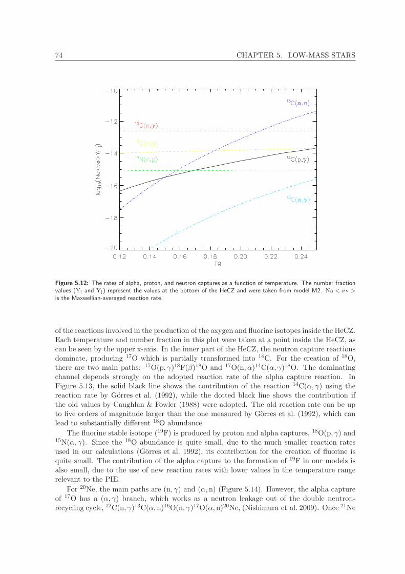
74 CHAPTER 5. LOW-MASS STARS
Figure 5.12: The rates of alpha, proton, and neutron captures as a function of temperature. The number fractionvalues (Yi and Yj) represent the values at the bottom of the HeCZ and were taken from model M2. Na < σv >is the Maxwellian-averaged reaction rate.
of the reactions involved in the production of the oxygen and fluorine isotopes inside the HeCZ.Each temperature and number fraction in this plot were taken at a point inside the HeCZ, ascan be seen by the upper x-axis. In the inner part of the HeCZ, the neutron capture reactionsdominate, producing 17O which is partially transformed into 14C. For the creation of 18O,there are two main paths: 17O(p, γ)18F(β)18O and 17O(n, α)14C(α, γ)18O. The dominatingchannel depends strongly on the adopted reaction rate of the alpha capture reaction. InFigure 5.13, the solid black line shows the contribution of the reaction 14C(α, γ) using thereaction rate by Gorres et al. (1992), while the dotted black line shows the contribution ifthe old values by Caughlan & Fowler (1988) were adopted. The old reaction rate can be upto five orders of magnitude larger than the one measured by Gorres et al. (1992), which canlead to substantially different 18O abundance.
The fluorine stable isotope (19F) is produced by proton and alpha captures, 18O(p, γ) and15N(α, γ). Since the 18O abundance is quite small, due to the much smaller reaction ratesused in our calculations (Gorres et al. 1992), its contribution for the creation of fluorine isquite small. The contribution of the alpha capture to the formation of 19F in our models isalso small, due to the use of new reaction rates with lower values in the temperature rangerelevant to the PIE.
For 20Ne, the main paths are (n, γ) and (α, n) (Figure 5.14). However, the alpha captureof 17O has a (α, γ) branch, which works as a neutron leakage out of the double neutron-recycling cycle, 12C(n, γ)13C(α, n)16O(n, γ)17O(α, n)20Ne, (Nishimura et al. 2009). Once 21Ne
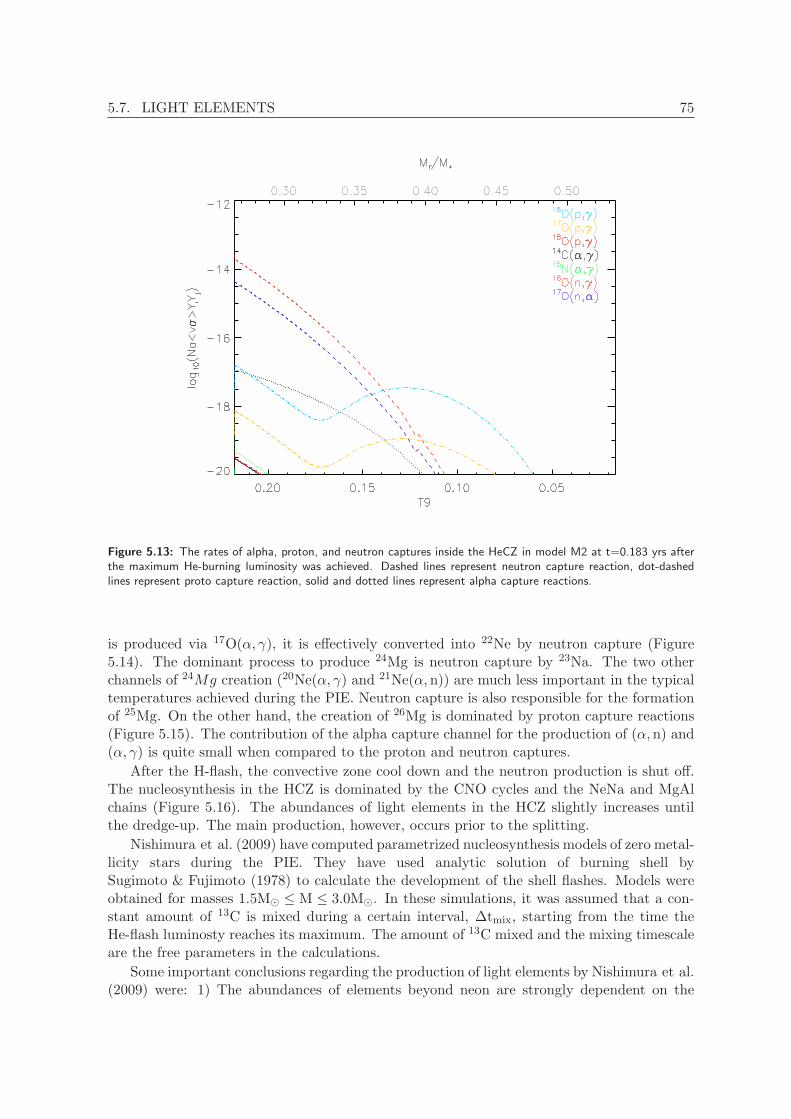
5.7. LIGHT ELEMENTS 75
Figure 5.13: The rates of alpha, proton, and neutron captures inside the HeCZ in model M2 at t=0.183 yrs afterthe maximum He-burning luminosity was achieved. Dashed lines represent neutron capture reaction, dot-dashedlines represent proto capture reaction, solid and dotted lines represent alpha capture reactions.
is produced via 17O(α, γ), it is effectively converted into 22Ne by neutron capture (Figure5.14). The dominant process to produce 24Mg is neutron capture by 23Na. The two otherchannels of 24Mg creation (20Ne(α, γ) and 21Ne(α, n)) are much less important in the typicaltemperatures achieved during the PIE. Neutron capture is also responsible for the formationof 25Mg. On the other hand, the creation of 26Mg is dominated by proton capture reactions(Figure 5.15). The contribution of the alpha capture channel for the production of (α, n) and(α, γ) is quite small when compared to the proton and neutron captures.
After the H-flash, the convective zone cool down and the neutron production is shut off.The nucleosynthesis in the HCZ is dominated by the CNO cycles and the NeNa and MgAlchains (Figure 5.16). The abundances of light elements in the HCZ slightly increases untilthe dredge-up. The main production, however, occurs prior to the splitting.
Nishimura et al. (2009) have computed parametrized nucleosynthesis models of zero metal-licity stars during the PIE. They have used analytic solution of burning shell bySugimoto & Fujimoto (1978) to calculate the development of the shell flashes. Models wereobtained for masses 1.5M⊙ ≤ M ≤ 3.0M⊙. In these simulations, it was assumed that a con-stant amount of 13C is mixed during a certain interval, ∆tmix, starting from the time theHe-flash luminosty reaches its maximum. The amount of 13C mixed and the mixing timescaleare the free parameters in the calculations.
Some important conclusions regarding the production of light elements by Nishimura et al.(2009) were: 1) The abundances of elements beyond neon are strongly dependent on the

76 CHAPTER 5. LOW-MASS STARS
Figure 5.14: Same as Figure 5.13 for neon isotopes.
Figure 5.15: Same as Figure 5.13 for magnesium isotopes.
amount of mixed 13C (which is an indicative of the amount of protons mixed), while oxy-gen, fluorine, and neon isotopes are mildly dependent on this property. 2) The abundancepatterns are almost independent of the mixing duration if it is sufficiently long. If ∆tmix is
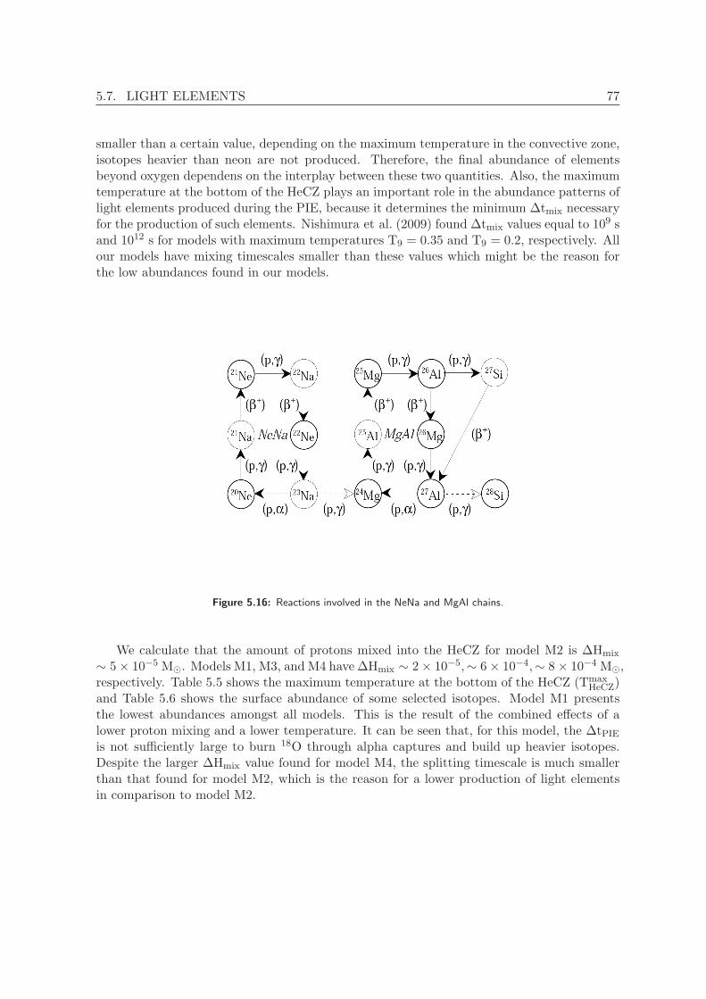
5.7. LIGHT ELEMENTS 77
smaller than a certain value, depending on the maximum temperature in the convective zone,isotopes heavier than neon are not produced. Therefore, the final abundance of elementsbeyond oxygen dependens on the interplay between these two quantities. Also, the maximumtemperature at the bottom of the HeCZ plays an important role in the abundance patterns oflight elements produced during the PIE, because it determines the minimum ∆tmix necessaryfor the production of such elements. Nishimura et al. (2009) found ∆tmix values equal to 109 sand 1012 s for models with maximum temperatures T9 = 0.35 and T9 = 0.2, respectively. Allour models have mixing timescales smaller than these values which might be the reason forthe low abundances found in our models.
Figure 5.16: Reactions involved in the NeNa and MgAl chains.
We calculate that the amount of protons mixed into the HeCZ for model M2 is ∆Hmix
∼ 5× 10⁻⁵ M⊙. Models M1, M3, and M4 have ∆Hmix ∼ 2× 10⁻⁵,∼ 6× 10⁻⁴,∼ 8× 10⁻⁴ M⊙,respectively. Table 5.5 shows the maximum temperature at the bottom of the HeCZ (Tmax
HeCZ)and Table 5.6 shows the surface abundance of some selected isotopes. Model M1 presentsthe lowest abundances amongst all models. This is the result of the combined effects of alower proton mixing and a lower temperature. It can be seen that, for this model, the ∆tPIEis not sufficiently large to burn 18O through alpha captures and build up heavier isotopes.Despite the larger ∆Hmix value found for model M4, the splitting timescale is much smallerthan that found for model M2, which is the reason for a lower production of light elementsin comparison to model M2.
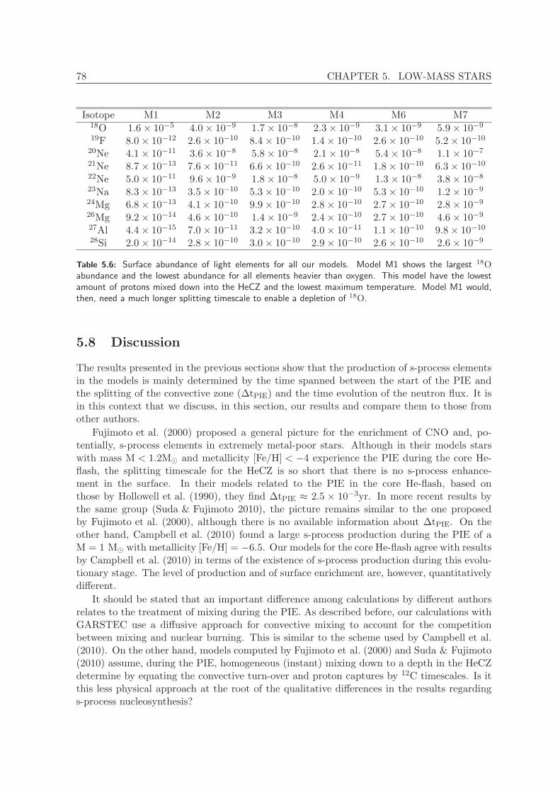
78 CHAPTER 5. LOW-MASS STARS
Isotope M1 M2 M3 M4 M6 M718O 1.6× 10⁻⁵ 4.0× 10⁻⁹ 1.7× 10⁻⁸ 2.3× 10⁻⁹ 3.1× 10⁻⁹ 5.9× 10⁻⁹
19F 8.0× 10⁻¹² 2.6× 10⁻¹⁰ 8.4× 10⁻¹⁰ 1.4× 10⁻¹⁰ 2.6× 10⁻¹⁰ 5.2× 10⁻¹⁰
20Ne 4.1× 10⁻¹¹ 3.6× 10⁻⁸ 5.8× 10⁻⁸ 2.1× 10⁻⁸ 5.4× 10⁻⁸ 1.1× 10⁻⁷
21Ne 8.7× 10⁻¹³ 7.6× 10⁻¹¹ 6.6× 10⁻¹⁰ 2.6× 10⁻¹¹ 1.8× 10⁻¹⁰ 6.3× 10⁻¹⁰
22Ne 5.0× 10⁻¹¹ 9.6× 10⁻⁹ 1.8× 10⁻⁸ 5.0× 10⁻⁹ 1.3× 10⁻⁸ 3.8× 10⁻⁸
23Na 8.3× 10⁻¹³ 3.5× 10⁻¹⁰ 5.3× 10⁻¹⁰ 2.0× 10⁻¹⁰ 5.3× 10⁻¹⁰ 1.2× 10⁻⁹
24Mg 6.8× 10⁻¹³ 4.1× 10⁻¹⁰ 9.9× 10⁻¹⁰ 2.8× 10⁻¹⁰ 2.7× 10⁻¹⁰ 2.8× 10⁻⁹
26Mg 9.2× 10⁻¹⁴ 4.6× 10⁻¹⁰ 1.4× 10⁻⁹ 2.4× 10⁻¹⁰ 2.7× 10⁻¹⁰ 4.6× 10⁻⁹
27Al 4.4× 10⁻¹⁵ 7.0× 10⁻¹¹ 3.2× 10⁻¹⁰ 4.0× 10⁻¹¹ 1.1× 10⁻¹⁰ 9.8× 10⁻¹⁰
28Si 2.0× 10⁻¹⁴ 2.8× 10⁻¹⁰ 3.0× 10⁻¹⁰ 2.9× 10⁻¹⁰ 2.6× 10⁻¹⁰ 2.6× 10⁻⁹
Table 5.6: Surface abundance of light elements for all our models. Model M1 shows the largest 18Oabundance and the lowest abundance for all elements heavier than oxygen. This model have the lowestamount of protons mixed down into the HeCZ and the lowest maximum temperature. Model M1 would,then, need a much longer splitting timescale to enable a depletion of 18O.
5.8 Discussion
The results presented in the previous sections show that the production of s-process elementsin the models is mainly determined by the time spanned between the start of the PIE andthe splitting of the convective zone (∆tPIE) and the time evolution of the neutron flux. It isin this context that we discuss, in this section, our results and compare them to those fromother authors.
Fujimoto et al. (2000) proposed a general picture for the enrichment of CNO and, po-tentially, s-process elements in extremely metal-poor stars. Although in their models starswith mass M < 1.2M⊙ and metallicity [Fe/H] < −4 experience the PIE during the core He-flash, the splitting timescale for the HeCZ is so short that there is no s-process enhance-ment in the surface. In their models related to the PIE in the core He-flash, based onthose by Hollowell et al. (1990), they find ∆tPIE ≈ 2.5 × 10⁻³yr. In more recent results bythe same group (Suda & Fujimoto 2010), the picture remains similar to the one proposedby Fujimoto et al. (2000), although there is no available information about ∆tPIE. On theother hand, Campbell et al. (2010) found a large s-process production during the PIE of aM = 1 M⊙ with metallicity [Fe/H] = −6.5. Our models for the core He-flash agree with resultsby Campbell et al. (2010) in terms of the existence of s-process production during this evolu-tionary stage. The level of production and of surface enrichment are, however, quantitativelydifferent.
It should be stated that an important difference among calculations by different authorsrelates to the treatment of mixing during the PIE. As described before, our calculations withGARSTEC use a diffusive approach for convective mixing to account for the competitionbetween mixing and nuclear burning. This is similar to the scheme used by Campbell et al.(2010). On the other hand, models computed by Fujimoto et al. (2000) and Suda & Fujimoto(2010) assume, during the PIE, homogeneous (instant) mixing down to a depth in the HeCZdetermine by equating the convective turn-over and proton captures by 12C timescales. Is itthis less physical approach at the root of the qualitative differences in the results regardings-process nucleosynthesis?

5.8. DISCUSSION 79
Different neutron fluxes lead to different s-process paths. Campbell et al. (2010) found aneutron superburst already at the beginning of the PIE, achieving maximum neutron densityvalues of ∼ 1015cm−3, which immediately produces large amounts of s-process elements. Onthe other hand, in our models, as the ingestion of protons progresses, the neutron densityincreases smoothly up to values above 1014cm−3 (see Figure 5.5). This results in a slowerproduction of s-process in the HeCZ than the one found by Campbell et al. (2010). Also,the larger size of our convective zone contributes to effectively slow down the production ofs-process elements. The combination of a slower production and a shorter timescale for thesplitting leads to surface abundances lower than those reported by Campbell et al. (2010):for instance, their Sr surface abundance is more than 2 dex larger than ours (Table 5.7). Wenote here that Campbell et al. (2010) had to extrapolate their results because of numericalproblems which did not allow them to follow the dredge-up of processed material into thestellar envelope. On the contrary, our results are based on full models that follow in detailthe enrichment of the stellar surface as a consequence of the merging between the HCZ andthe convective envelope following the PIE. Although we do not believe the difference in thefinal enrichement are caused because of extrapolations done by Campbell et al. (2010) (basedon reasonable assumptions), it is clear our calculations represent a qualitative step forwardin modelling the PIE and subsequent enrichment of stellar envelopes.
We have compared our models with the hyper metal-poor (HMP) stars HE1327-2326and HE0107-5240. It is clear that the self-pollution scenario cannot explain the abundancepatterns observed in HE0107-5240 (this scenario is not suitable to HE1327-2326 since thisstar is not a giant and has not undergone the He-core flash yet): our models produce ∼ 3dex more [C/Fe] and at least 2 dex more Sr and Ba than observed in HE0107-5240 (see bluesquares and black solid line in Fig. 5.17). In the binary scenario, on the other hand, there isno restriction to the evolutionary stage of the observed star and we can compare our modelswith both stars. In this scenario, material is transferred from the primary star (representedhere by our models) and is expected to be diluted in the envelope of the companion star (theobserved star). We assumed an initial solar-scaled composition of the same metallicity as ourmodel M2 for the observed star and diluted the surface composition obtained in our modelswith this material by a factor that would match the resulting carbon abundance ([C/Fe])to the observed value. This factor, fD, represents the fractional mass of accreted materialwith respect to the mass of the accreting star over which the polluting material is mixed.Therefore, we used dilution factors fD = 2× 10⁻³ and fD = 6× 10⁻³ for HE1327-2326 andHE0107-5240, respectively.
Figure 5.17 shows the abundances derived for the two HMP stars along with the pre-dictions from our models. Comparing with HE1327-2326 abundances, our model includingdilution (see red symbols and red dashed line in Fig. 5.17), which by definition matches theobserved C abundance, underproduces N by a factor of 7 and O by a factor of 9. The other el-ements shown in Fig. 5.17 are all underproduced by factors larger than 10 in comparison withthe observations, except lithium. One interesting signature of the PIE is the 7Li production(Iwamoto et al. 2004; Cristallo et al. 2009a). Our models produce Li surface abundance morethan two orders of magnitude larger than the Spite plateau (Spite & Spite 1982). Therefore,Li is overproduced when comparing the diluted values with those observed in the HMP stars(Fig. 5.17). In any case, we do not account for the possibility that Li may be (partially)destroyed after being accreted.
For HE0107-5240 our model including dilution produces oxygen in agreement with theobserved values, while N is strongly overproduced by a factor of ∼ 60. Na, Mg, Al, Ca,

80 CHAPTER 5. LOW-MASS STARS
Ti, and Ni are underproduced in our models, however, they could come from an early su-pernova that polluted the cloud (blue symbols and blue dashed line in Fig. 5.17). For Srand Ba observations allow only the determination of upper values for their abundances. Ourmodel predicts abundances for these elements a factor of 4 smaller than the observed limits.Nishimura et al. (2009) have done a parameterized study of the PIE in zero metallicity stars.They parameterized the amount of 13C mixed and the duration of the mixing epoch. Theysuggested that the primary star that polluted HE0107-5240 should have a mass in the range1.5M⊙ < M < 3.0M⊙ and therefore suffered PIE during the AGB phase. Our models showthat stars with smaller masses should not be discarded as the source of carbon and s-processenhancement for this star.
In our simple dilution model, we have assumed that mass was transferred before the starentered the AGB phase. Low-mass stars that suffered PIE during the core He-flash undergoa normal AGB evolution, i.e., there is no PIE during this phase. Therefore, the productionof s-process elements should happen in a radiative environment if a 13C pocket is formed.We might speculate on the possible consequence if the primary had not transferred mass tothe companion star right after the PIE but rather during or after its AGB evolution. Themain products carried to the surface after the third dredge-up (TDU) are carbon and s-process elements. Hence, before transferring mass, the primary would be even more enrichedin these elements than prior to this phase. Nitrogen abundance would remain the same sinceHot Bottom Burning (HBB) does not happen in stars with masses M = 1 M⊙ and Li wouldbe depleted during the TDU. In this way, a better match to the nitrogen and the lithiumabundances of HE 0107-5240 could be obtained if the accreted mass is small enough. Also, the12C/13C ratio would increase during the AGB evolution and could better match the observedlower limit for HE 0107-5240 (12C/13C > 50).
Element M2 M3 M4 M6 M7
C 6.49 6.24 6.44 6.82 5.69N 6.80 6.34 6.96 6.94 5.81O 5.39 5.13 5.46 5.71 4.58Sr 1.67 2.32 2.08 2.71 1.88Y 2.04 2.58 2.45 3.11 2.23Zr 2.14 2.78 2.59 3.26 2.33Ba 3.37 3.65 3.85 4.30 3.13La 3.69 3.72 4.15 4.39 3.24Eu 3.33 3.36 3.79 4.08 2.18Pb 5.02 5.05 4.93 4.82 5.31
Table 5.7: Surface abundances given in terms of: [X/Fe] = log10(X/Fe)⋆ − log10(X/Fe)⊙.
Concerning our zero metallicity model, we have found that only elements lighter than ironhave been produced. In the viewpoint of the binary pollution scenario, this result does notsupport a low-mass zero metallicity star as the polluting companion of the two HMP starsdiscussed in this paper, if mass is transferred before it enters the AGB evolution.
In closing the discussion, we have done a simple test to determine if the productionof s-process elements during the PIE is sensitive to the stellar mass. As stated before,Fujimoto et al. (2000) has found an upper limit of 1.2 M⊙ for the occurrence of the PIE.
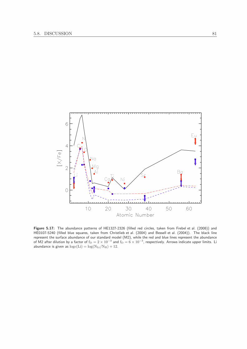
5.8. DISCUSSION 81
Figure 5.17: The abundance patterns of HE1327-2326 (filled red circles, taken from Frebel et al. (2008)) andHE0107-5240 (filled blue squares, taken from Christlieb et al. (2004) and Bessell et al. (2004)). The black linerepresent the surface abundance of our standard model (M2), while the red and blue lines represent the abundanceof M2 after dilution by a factor of fD = 2× 10⁻³ and fD = 6× 10⁻³, respectively. Arrows indicate upper limits. Liabundance is given as logǫ(Li) = log(NLi/NH) + 12.

82 CHAPTER 5. LOW-MASS STARS
On the low-mass range, we have computed the evolution of a 0.82 M⊙ and Z=10−8 model(representative of the lowest stellar mass that has had time to evolve to the core He-flashin the lifetime of the Milky Way) and found that, in comparison to model M2, the splittingtime is a factor of 3 shorter (∆tPIE =∼ 0.08 yr), but still more than 30 times larger thanmodels by Hollowell et al. (1990). The neutron flux increases more rapidly than in model M2and just 0.03 yr after LHe
max, the neutron density at the bottom of the HeCZ is already largerthan 1014 cm−3. As a result we find that, associated with the PIE, there is a total neutronexposure at the bottom the HeCZ of 130 mbarn−1 and an average neutron exposure overthe whole HeCZ of 30 mbarn−1. We have performed post-processing nucleosynthesis for thismodel. The abundance pattern during the HeCZ is very similar to model M2 (and common toall models of equal metallicity undergoing the core He-flash) and the neutron exposure verylarge and within a factor of 2 of model M2. As can be seen in Table 5.7, s-process elements areefficiently produced with a abundance pattern more prominent towards the first and seconds-process peak than model M2 due to its lower neutron exposure.
At the end of the PhD, it was realized that interpolation in metallicity used in GARSTECunderestimates the opacity for 0 < Z < 10−4. Although a test model showed that this causeddifference in the results presented in this chapter, the differences are not sufficient high tochange the main results and conclusions presented here.
5.9 Conclusions
We have performed evolutionary calculations for low-mass EMP and zero metallicity stars.Our models follow the proton ingestion episode (PIE) during the core He-flash and the sub-sequent hydrogen flash. We have then used these calculations as input to a post-processingunit, where we have performed calculations of s-process nucleosynthesis. A comparison withand among similar calculations found in the literature shows that the location at which theHe-flash occurs varies among different stellar codes (varying from 0.15 (Schlattl et al. 2001),∼ 0.26 this paper to 0.41 (Hollowell et al. 1990)). This is indicative of the uncertainties instellar modeling and is likely to impact results of the PIE modeling.
The production of s-process elements and subsequent surface enrichment during the PIEin EMP low-mass stars depends strongly on the efficiency of the convective mixing and onthe general properties of the PIE (for instance, ∆tPIE). We do find large production of s-process elements in our models. The surface abundances after dredge- up are, however, about2 dex smaller than those reported by Campbell et al. (2010). This is likely the result of thedifference in the neutron density history between our models and those by Campbell et al.(2010); we do not find the neutron superburst reported by these authors. In more detail, ourmodels produce 2-3 dex less first and second peak s-process elements whereas Pb productionis smaller in our models by 1.3 dex. On the other hand, our results qualitatively agree thats-process production happens during the PIE in the core-He flash phase, which is in contrastwith (Fujimoto et al. 2000; Suda & Fujimoto 2010) results who found no relevant s-processproduction during the PIE.
Our models produce C, N, and O surface abundances 2-3 dex larger than the abundancevalues observed in the HMP stars. The high CNO abundances in our models disfavor theself-enrichment scenario to explain the EMP abundance patterns, as other works on the topichave shown before. In the viewpoint of the mass-transfer scenario, our models support theidea that a low-mass star can be the donor star because the dilution of the transferred material

5.9. CONCLUSIONS 83
occurs in the secondary star envelope. In fact, our estimation of the dilution factors during theaccretion process shows that the secondary needs to accrete a mass equal to only a few partsper thousand of its own envelope mass in order to match the observed carbon abundances.
Based on our results, and in qualitative agreement with those from Campbell et al. (2010),we conclude that stars with masses M ≤ 1 M⊙ cannot be excluded as the binary companions ofthe two most iron deficient stars yet observed. In addition, the latest findings by Caffau et al.(2011, 2012) push the lowest metallicity at which low mass stars can form, increasing the needof detailed models for this class of stars. All these results reinforce the necessity of detailedstudies of the PIE, both with hydrodynamic simulations and stellar evolutionary models, inorder to achieve a more realistic picture of the its properties.

84 CHAPTER 5. LOW-MASS STARS

Chapter 6Intermediate-Mass Stars
6.1 Models
We have performed evolutionary calculations from the zero-age main-sequence to the TP-AGB phase. The composition is solar-scaled with metallicities Z=0, Z = 10−8, Z = 10−7, andZ = 10−5. Our standard models (I1, I2, I3, I7, I8, I9, I10, I11, I12 ) include overshooting,with the standard choice of the free parameter f = 0.016 (see Chapter 5 for more details),and low-temperature opacities with varying C/O ratio. Convection is modeled using theMixing Length Theory (MLT) and the mixing length parameter α = 1.75, similar to theone obtained from standard solar model calculations. Mass-loss is included as described inChapter 3. OPAL equation of state (Rogers et al. 1996) was used. Radiative opacity tablesare also from OPAL Iglesias & Rogers (1996). We have used the results by Itoh et al. (1983)for electron conduction opacities. For these models we have used updated reaction rates inthe GARSTEC network. Most of the rates for the proton capture and some alpha capturereactions are from the newest compilation by Iliadis et al. (2010). The 3α reaction rate istaken from Fynbo et al. (2005).
In order to verify the impact of the main uncertanties in AGB modelling in the finalcomposition, we have performed extra models using: 1) fixed C/O opacities, 2) the mass-lossrate according to Bloecker (1995), and 3) smaller overshooting parameter.

86 CHAPTER 6. INTERMEDIATE-MASS STARS
Model Mass(M⊙) Z
I1 1.5 10−8 StdI2 2.0 zero StdI3 2.0 10−8 StdI4 2.0 10−8 fixed opacityI5 2.0 10−8 f=0.008I6 2.0 10−8 BL95 mass-lossI7 2.0 10−7 StdI8 2.0 10−5 StdI9 3.0 zero StdI10 3.0 10−8 StdI11 3.0 10−7 StdI12 3.0 10−5 Std
Table 6.1: List of intermediate-mass stars models.
6.2 From ZAMS to the TP-AGB
In Pop. I and II1 intermediate-mass (IM) stars, the H-burning during the MS is dominatedby the CNO cycles. The path followed by these stars, during the MS, in the HRD is differentfrom that followed by low-mass (LM) stars. While in the LM case the star moves towardslarger effective temperatures (Teff) and luminosities, the IM star increases its luminositytowards lower Teff . In EMP and zero metallicity stars, due to the absence of CNO catalysts,the CNO cycles cannot operate and H-burning is then dominated by the p-p chains. Thisresults in a significant change in the MS morphology of these stars. Figure 6.1 displays theevolution of our standard models in the HRD. As it can be seen, the MS path is similar tothat followed by LM stars, as a result of the H-burning being powered by p-p chains.
In the zero metallicity models, the CNO cycles contribute to the H-burning only at theend of the MS. When the star reaches the turn-off, there is still a small amount of H in thecore (XH ∼ 10−2). The temperature in the core is high enough to trigger some He-burningand to produce 12C. Once the 12C abundance reaches ∼ 10−12, a thermal runaway takes placeand a small convective core is formed. The CNO flash can be seen in the HRD as a small loopat the turn-off (Figure 6.1). Figure 6.2 shows how the star reacts to the onset of the thermalrunaway by the end of the MS. The density decreases, while the temperature is kept almostconstant due to the expansion of the core. The now convective core, dredge-down new fuel,prolonging the MS in this model.
For a given mass, the different degrees of CNO catalysts result in large differences in theturn-off (TO) luminosities (up to ∼ 0.25 dex in models with 3.0M⊙ and ∼ 0.4 dex in modelswith 2.0M⊙). The larger the initial abundance of CNO elements, the faster their contributionto the H-burning increases and, thus, the smaller is the TO luminosity. The TO temperaturesare also larger in models with less CNO catalysts, however, the difference between the models,in this metallicity range, is more modest (< 0.05 dex). The 3.0M⊙ model with metallicity
1Population I stars are young metal-rich stars. The Sun is an example of Pop. I star. They are found inthe Disk of our Galaxy. Pop. II, on the other hand, are old metal-poor stars found mainly in the Halo. Pop.III are the primordial stars, without any metal.

6.2. FROM ZAMS TO THE TP-AGB 87
Figure 6.1: HR Diagram of intermediate-mass stars for our standard models. There are significant differencesbetween EMP and Z=0 stars and the Pop I and II MS of IM stars. The arrow indicates the position of the CNOflash in model I9. Numbers indicate the initial stellar mass in M⊙.
Z = 10−5 have a different TO morphology: it presents a hook-like feature. This kind ofstructure indicates that a prominent convective core was formed due to the high efficiency ofthe CNO cycles in this model.
Almost all models avoid the RGB configuration (except model I8) and the core He-burninghappens at lower central densities than those experienced by stars with larger metallicities.Moreover, due to the lack of the RGB configuration, the star only experiences one dredge-upepisode: the second dredge-up (SDU). The main product brought-up to the surface by theSDU is He. The amount by which its abundance increases depends on the initial mass and themetallicity. The lower the metallicity, the larger the helium abundance after SDU. Figures 6.3and 6.4 show the abundance profiles of hydrogen, helium and some CNO isotopes just beforeSDU sets in. It can be seen that SDU goes deeper in the zero metallicity models, reachinglayers richer in helium than the model with Z = 10−8. For models with the same metallicity,the larger the initial mass, the larger the helium abundance (Table 6.2). In comparison toother works in the literature (Campbell 2007; Suda & Fujimoto 2010), our He abundancesagree with their values within less than 8% for any initial mass and metallicity. For instance,we found that the He mass-fraction increases from its initial value Y=0.245 to 0.309 in our2.0M⊙ model with zero metallicity, while Campbell (2007) and Suda & Fujimoto (2010) foundY = 0.31 and Y = 0.29, respectively.
Regarding the 12C/13C ratio, in the IM models the ratio decreases from an initial value∼ 80 to similar values independent of the metallicity. In contrast, models with zero metallcity
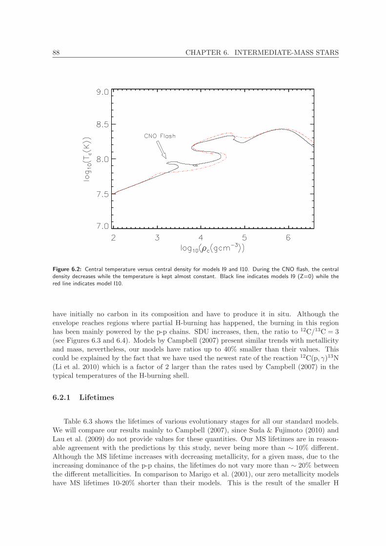
88 CHAPTER 6. INTERMEDIATE-MASS STARS
Figure 6.2: Central temperature versus central density for models I9 and I10. During the CNO flash, the centraldensity decreases while the temperature is kept almost constant. Black line indicates models I9 (Z=0) while thered line indicates model I10.
have initially no carbon in its composition and have to produce it in situ. Although theenvelope reaches regions where partial H-burning has happened, the burning in this regionhas been mainly powered by the p-p chains. SDU increases, then, the ratio to 12C/13C = 3(see Figures 6.3 and 6.4). Models by Campbell (2007) present similar trends with metallicityand mass, nevertheless, our models have ratios up to 40% smaller than their values. Thiscould be explained by the fact that we have used the newest rate of the reaction 12C(p, γ)13N(Li et al. 2010) which is a factor of 2 larger than the rates used by Campbell (2007) in thetypical temperatures of the H-burning shell.
6.2.1 Lifetimes
Table 6.3 shows the lifetimes of various evolutionary stages for all our standard models.We will compare our results mainly to Campbell (2007), since Suda & Fujimoto (2010) andLau et al. (2009) do not provide values for these quantities. Our MS lifetimes are in reason-able agreement with the predictions by this study, never being more than ∼ 10% different.Although the MS lifetime increases with decreasing metallicity, for a given mass, due to theincreasing dominance of the p-p chains, the lifetimes do not vary more than ∼ 20% betweenthe different metallicities. In comparison to Marigo et al. (2001), our zero metallicity modelshave MS lifetimes 10-20% shorter than their models. This is the result of the smaller H

6.2. FROM ZAMS TO THE TP-AGB 89
Figure 6.3: Upper panel: The hydrogen (Red line) and helium (Black line) abundances profile before the occurrenceof the SDU in model I9. Lower panel: Same as the upper panel for some CNO isotopes. The dotted vertical linerepresents the maximum depth of the envelope during the SDU.
Figure 6.4: Upper panel: The hydrogen (Red line) and helium (Black line) abundances profile before the occurrenceof the SDU in model I10. Lower panel: Same as the upper panel for some CNO isotopes. The dotted vertical linerepresents the maximum depth of the envelope during the SDU.

90 CHAPTER 6. INTERMEDIATE-MASS STARS
Model Y 12C/13C
I1 0.265 23I2 0.309 3I3 0.295 18I7 0.286 18I8 0.264 17I9 0.353 3I10 0.325 15I11 0.300 15I12 0.264 15
Table 6.2: The surface abundances after SDU for all our standard models.
content in our models.
Model tMS tSGB tRGB tCHeB
I1 1465 102 zero 150I2 634(-3) 15(-20) zero 37(+23)I3 581(-7) 52(+20) zero 44(+10)I7 553(-9) 91(+57) zero 55(+10)I8 516(+5) 115(-18) 3(-47) 93(-2)I9 191(-13) 7(-13) zero 12(0)I10 176(-7) 22(+5) zero 19(+12)I11 179(+1) 36(+20) zero 27(+13)I12 185(0) 11(+39) zero 48(+2)
Table 6.3: Lifetimes of various evolutionary stages for all our standard models. All ages are given in Myr.tMS: lifetime for the main sequence, tSGB: lifetime for the subgiant branch, tRGB: lifetime for the redgiant branch, and tCHeB lifetime for the core He-burning. The numbers in the parenthesis indicate thedifferences (in percentage) between our lifetimes and those by Campbell (2007)
Following Campbell (2007), the SGB lifetime was defined, in the cases where there is noRGB, as the time between the turn-off and the He-burning ignition in the core. For the 2.0M⊙
models, there is an increase in the SGB lifetime with metallicity. The lower the metallicity,the lower is the density at which He-burning is ignited in the core. For the 3.0M⊙ models, theSGB lifetimes increase with metallicity up to a threshold above which the lifetimes decrease(our most metal-rich model - I12). This is probably related to the efficient convective coreoccurring in the MS of this model. In spite of the similar behaviour with metallicity andinitial mass, the differences between our lifetimes and those by Campbell (2007) varies from 5up to 57% in this evolutionary stage. The core He-burning, on the other hand, is consistentlylonger in our models. This can be explained by the inclusion of overshooting in our modelsthat brings more fuel to the core, prolonging the He-burning phase.

6.3. PROTON INGESTION EPISODE 91
6.3 Proton Ingestion Episode
As explained in Chapter 2, in IM stars PIE occurs at the beginning of the TP-AGB phase.In Figure 6.5 we show the evolution of one of our zero metallicity models (I2). PIE occursafter a series of weak pulses at the beginning of the evolution. Similarly to the LM case,the PIE is characterized by a peak in the H-burning luminosity (Figure 6.5). The He-flash,now in a shell, induces the formation of a convective zone (HeCZ) that breaks through theH-He discontinuity due to the low entropy barrier between the H and He layers. Protons are,then, dredge-down into the HeCZ and burnt at high temperatures, resulting in a secondaryflash: the H-flash. It can be seen in Figure 6.5 that following the PIE the envelope deepensdown and dredges-up material from the former HeCZ, increasing the surface abundance ofCNO elements. The amount by which the envelope is enriched is smaller than in the LMcase. While PIE in LM stars increases the CNO abundance to XCNO > 10−2, in IM stars theincrease is more modest (XCNO ∼ 10−4 − 10−3 - See Tab.6.4). Once the metal content in theenvelope reaches values of Z ∼ 10−4, the TP-AGB evolution proceeds as in Pop.I and II stars.
Figure 6.5: Upper panel: Time evolution of the surface abundance of the CNO elements in model I2. Bottompanel: Evolution along the AGB of the H-burning (Black Line) and the He-burning (Red line) luminosities.
Figure 6.6 shows the evolution of the convective regions from the formation of the HeCZto the post-PIE dredge-up. The outer border of the HeCZ reaches H-rich regions, about 80yrs after the formation of the HeCZ, and dredges-down protons into this zone. The H-flashcauses a splitting of the HeCZ into two convective zone. The Hydrogen Convetive Zone (HCZ)continues expanding until the envelope deepens down and products of the nucleosynthesis

92 CHAPTER 6. INTERMEDIATE-MASS STARS
during the PIE are transported to the surface.
Figure 6.6: An example of PIE during the TP-AGB: Evolution of the convective zone during the PIE of the 2.0M⊙
model with Z = 10−8. t0 is the time at which the convective zone is formed. Blue line is the position of maximumenergy released by H-burning. Red line is the position of maximum energy released by He-burning.
In our LM models, we have shown that during the PIE a large amount of neutrons areproduced. This neutron production should happen in a similar way to that of LM stars.When protons are dredge-down into the HeCZ, 13C is produced through proton capture by12C. The abundant 4He is then captured by the newly produced 13C, releasing neutrons intothe convective zone. Iwamoto et al. (2004) have speculated the possibility of s-processingduring the PIE at the TP-AGB. They have found neutron densities larger than 1013cm−3 atthe bottom of the HeCZ in their models. Using a network that included neutron productionreaction, Campbell (2007) have found neutron production during the PIE. Our models agreewith these studies, since they also show large amounts of neutrons inside the HeCZ. Figure6.7 shows the abundance profile of some selected isotopes during the PIE in the HeCZ ofmodel I7. As expected, neutrons were produced in a large amount (Nmax
n ∼ 1012cm−3) duringthis phenomenon.
6.3.1 Comparison with the literature
We will compare our models mainly to the works by Campbell (2007), Lau et al. (2009), andSuda & Fujimoto (2010) (see Figure 6.8). PIE happens in all our models. For the modelswith 2.0M⊙, we find that PIE occurs during the TP-AGB for metallicities up to Z = 10−5.This is in agreement with the results by Suda & Fujimoto (2010) and Campbell (2007) that

6.3. PROTON INGESTION EPISODE 93
Figure 6.7: Chemical composition of the HeCZ during the PIE before the H-flash. To show the neutron abundance inthe plot we added 12 to the logarithm of the neutron mass-fraction, therefore the real maximum neutron abundancein the HeCZ is Xn ∼ 10−16.
found PIE for metallicities [Fe/H] < −3.0. Nevertheless, for this initial mass Lau et al. (2009)models do not undergo PIE if [Fe/H] > −4.0. Furthermore, when overshooting is included intheir model, PIE is supressed at even lower metallicities (Z = 10−7).
Table 6.4 shows some properties of the PIE for all our models. The 2.0M⊙ models havecore masses between 0.01M⊙ and 0.05M⊙ smaller than those found by Campbell (2007) forsimilar metallicities. In comparison to models by Suda & Fujimoto (2010), our core massesare usually larger by less than 0.08M⊙. Regarding the H-flash ignition point, our modelshave MH
max smaller than the values found in Campbell (2007) models. This is probably aconsequence of the inclusion of overshooting in our models. For instance, model I5 which hasa smaller overshooting parameter has an H-flash ignition point 0.015M⊙ larger than modelI3. Another signature from our models that was already observed in the LM models is theinner position of the He-flash. Our models have inner ignition points than those found inthe literature. This can result in longer ingestion episodes which, in turn, should have animportant impact in the s-process production during the PIE.
For the 3.0M⊙ models, PIE occurs up to metallicities 10−5, however the model withZ = 10−5 suffers a weak PIE. The largest discrepancies in the literature are found for thisstellar mass. While Campbell (2007) found PIE for [Fe/H] < −4.0, Suda & Fujimoto (2010)metallicity boundary for the occurrence of the PIE is much smaller ([Fe/H] < −5.0). Lau et al.(2009), on the other hand, did not find PIE for any metallicity, but instead, their modelsundergo the carbon injection. In this phenomenon, a convective zone opens up on top of the
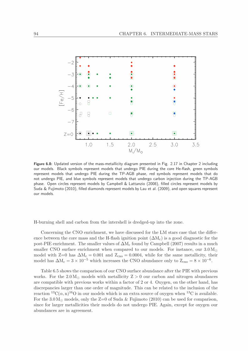
94 CHAPTER 6. INTERMEDIATE-MASS STARS
Figure 6.8: Updated version of the mass-metallicity diagram presented in Fig. 2.17 in Chapter 2 includingour models. Black symbols represent models that undergo PIE during the core He-flash, green symbolsrepresent models that undergo PIE during the TP-AGB phase, red symbols represent models that donot undergo PIE, and blue symbols represent models that undergo carbon injection during the TP-AGBphase. Open circles represent models by Campbell & Lattanzio (2008), filled circles represent models bySuda & Fujimoto (2010), filled diamonds represent models by Lau et al. (2009), and open squares representour models.
H-burning shell and carbon from the intershell is dredged-up into the zone.
Concerning the CNO enrichment, we have discussed for the LM stars case that the differ-ence between the core mass and the H-flash ignition point (∆Mc) is a good diagnostic for thepost-PIE enrichment. The smaller values of ∆Mc found by Campbell (2007) results in a muchsmaller CNO surface enrichment when compared to our models. For instance, our 3.0M⊙
model with Z=0 has ∆Mc = 0.001 and Zcno = 0.0004, while for the same metallicity, theirmodel has ∆Mc = 3× 10⁻⁵ which increases the CNO abundance only to Zcno = 8× 10⁻⁶.
Table 6.5 shows the comparison of our CNO surface abundance after the PIE with previousworks. For the 2.0M⊙ models with metallicity Z > 0 our carbon and nitrogen abundancesare compatible with previous works within a factor of 2 or 4. Oxygen, on the other hand, hasdiscrepancies larger than one order of magnitude. This can be related to the inclusion of thereaction 13C(α, n)16O in our models which is an extra source of oxygen when 13C is available.For the 3.0M⊙ models, only the Z=0 of Suda & Fujimoto (2010) can be used for comparison,since for larger metallicities their models do not undergo PIE. Again, except for oxygen ourabundances are in agreement.

6.3. PROTON INGESTION EPISODE 95
Model LHemax LH
max MHemax MHe
c MHmax ∆Mc ∆Mig ZCNO Ys
I1 6.371 11.09 0.504 0.549 0.544 0.005 0.045 0.0017 0.300I2 5.115 10.92 0.624 0.690 0.641 0.048 0.056 0.0016 0.326I3 5.551 11.03 0.622 0.640 0.639 0.001 0.018 0.0015 0.316I4 4.867 11.27 0.621 0.640 0.626 0.014 0.019 0.0022 0.321I5 5.526 10.77 0.628 0.651 0.641 0.010 0.023 0.0016 0.314I6 5.215 10.69 0.620 0.640 0.639 0.001 0.020 0.0010 0.315I7 5.736 11.10 0.636 0.656 0.652 0.004 0.020 0.0011 0.297I8 7.423 10.82 0.623 0.652 0.640 0.012 0.029 0.0045 0.269I9 5.971 11.10 0.784 0.791 0.789 0.002 0.007 0.0003 0.354I10 5.826 11.22 0.823 0.829 0.828 0.001 0.006 0.0005 0.326I11 6.346 11.16 0.831 0.836 0.833 0.003 0.005 0.0005 0.302I12 6.072 5.365 0.811 0.821 0.820 0.001 0.010 0.0004 0.265
Table 6.4: Main properties of the proton ingestion episode. LHemax and LH
max are the logarithm of themaximum He-burning luminosity and the maximum H-burning luminosity in units of solar luminosity, re-spectively. MHe
max is the position of maximum energy released by He-burning. MHec is the core mass.MH
max
is the position of maximum energy release by H-burning. ∆Mc is the distance, in mass, that the H-shellmoves inwards during the PIE. ∆Mig is the distance, in mass, between the He-flash ignition point and theH-shell. All masses are given in units of solar mass. ZCNO is the surface mass-fraction of CNO elements.Ys
is the surface helium abundance after the PIE.
6.3.2 S-process
It was discussed in Chapter 5 that during the PIE the amount of s-process elements producedis a function of the time integrated neutron flux, the neutron exposure, averaged over the entireconvective zone. The neutron exposure, in turn, depends on the neutron flux and on the timebetween the start of the proton mixing and the splitting of the HeCZ (∆tPIE). Figure 6.9 showsthe surface abundance distribution for all our standard models with metallicities Z ≥ 10−8
after the PIE. For models with metallicity 10−8 (I1, I3, and I10), the largest differences in theabundance distribution can be seen in model I10. This model has ∆tPIE three to two ordersof magnitude larger than models I1 and I3, respectively (See Table 6.6). S-process occurs inthe three models, however, only model I10 has enough time to increase the s-process elementsabundances in several orders of magnitude. The same bahaviour can be seen in models withmetallicity Z = 10−7 and Z = 10−5.
The lower the metallicity the lower the number of iron-peak seeds available for neutroncapture. If the same amount of neutrons are released in all the cases, the lower metallicitystars should produce a larger amount of heavier s-process than in the higher metallicity case,due to the larger neutron to seed ratio. Figure 6.10 shows the ratio between the differents-process components. During the PIE similar neutron densities are achieved at the bottomof the HeCZ by all models (Nn > 1012cm−3). From Figure 6.10 it can be seen that ∆tPIEplays a more important role in determining the final indices than the metallicity. The largerPIE timescale in models I7 and I8 results in larger s-process production than models I11 andI12, respectively. Moreover, the longer PIE timescale in model I8 in comparison to modelI7 leads to larger neutron exposures and, therefore, to the production of heavier s-processelements in this model.

96 CHAPTER 6. INTERMEDIATE-MASS STARS
Reference Mass [Fe/H] XC XN XO
This work 1.5 -6.3 9.80× 10⁻⁴ 7.40× 10⁻⁴ 3.90× 10⁻⁶
This work 2.0 −∞ 1.10× 10⁻³ 4.50× 10⁻⁴ 1.90× 10⁻⁵
Siess et al. (2002) 2.0 −∞ 3.38× 10⁻³ 6.72× 10⁻⁵ 8.52× 10⁻⁵
Suda & Fujimoto (2010) 2.0 −∞ 1.39× 10⁻⁴ 6.74× 10⁻⁵ 8.52× 10⁻⁵
This work 2.0 -6.3 1.00× 10⁻³ 5.00× 10⁻⁴ 4.50× 10⁻⁶
This work 2.0 −5.3 7.30× 10⁻⁴ 3.80× 10⁻⁴ 6.20× 10⁻⁶
Suda & Fujimoto (2010) 2.0 −5.0 9.36× 10⁻⁴ 8.87× 10⁻⁵ 3.64× 10⁻⁵
This work 2.0 −3.3 4.10× 10⁻³ 1.40× 10⁻⁴ 8.30× 10⁻⁴
Iwamoto et al. (2004) 2.0 −2.7 9.84× 10⁻⁴ 1.80× 10⁻⁴ 6.95× 10⁻⁵
Suda & Fujimoto (2010) 2.0 −3.0 1.36× 10⁻³ 1.08× 10⁻⁴ 6.23× 10⁻⁵
This work 3.0 −∞ 1.30× 10⁻⁴ 1.70× 10⁻⁴ 1.70× 10⁻⁷
Siess et al. (2002) 3.0 −∞ 3.38× 10⁻³ 6.72× 10⁻⁵ 8.52× 10⁻⁵
Suda & Fujimoto (2010) 3.0 −∞ 1.39× 10⁻⁴ 6.74× 10⁻⁵ 8.52× 10⁻⁵
This work 3.0 -6.3 3.50× 10⁻⁴ 1.40× 10⁻⁴ 2.00× 10⁻⁷
This work 3.0 −5.3 3.80× 10⁻³ 1.40× 10⁻⁴ 3.70× 10⁻⁶
Suda & Fujimoto (2010) 3.0 −5.0 2.10× 10⁻⁵ 4.47× 10⁻⁷ 6.32× 10⁻⁷
This work 3.0 −3.3 3.90× 10⁻³ 2.80× 10⁻⁵ 1.10× 10⁻⁵
Iwamoto et al. (2004) 3.0 −2.7 4.94× 10⁻⁵ 7.29× 10⁻⁶ 1.71× 10⁻⁵
Suda & Fujimoto (2010) 3.0 −3.0 1.34× 10⁻⁶ 4.34× 10⁻⁶ 8.93× 10⁻⁶
Table 6.5: Comparison of CNO abundances after the PIE with previous works. We focus on the work bySuda & Fujimoto (2010) because they provide the abundance right after the post-PIE dredge-up, whileother works only give the yields (Campbell & Lattanzio 2008) or the abundance in plots(Lau et al. 2009).
Model ∆tPIE ∆tdI1 2.6× 10⁻⁴ 57.17I2 3.0× 10⁻³ 11.33I3 4.1× 10⁻³ 8.53I4 1.1× 10⁻¹ 0.68I5 2.0× 10⁻² 6.14I6 3.5× 10⁻² 23.38I7 4.7× 10⁻¹ 4.68I8 7.4× 10⁻¹ 4.45I9 7.6× 10⁻³ 0.59I10 2.1× 10⁻¹ 0.20I11 7.0× 10⁻² 0.20I12 2.5× 10⁻¹ 15.50
Table 6.6: ∆tPIE: time between the onset of the PIE and the H-flash. ∆td: time between the H-flash andthe start of the post-PIE dredge-up. All times are given in yrs.
Another important property affecting the s-process production during the PIE is the sizeof the convective zone (∆Mig). In a convective environment, at each timestep the s-processproducts are mixed throughout the convective zone. This should lead to a smaller production

6.3. PROTON INGESTION EPISODE 97
Figure 6.9: Bottom Panel: Total surface abundance distribution of some selected elements heavier than 30Si afterthe PIE. Upper panel: The same as in the bottom panel, but relative to solar.
in comparison to a radiative s-process. As explained in Chapter 5, the average neutronexposure is the key quantity in the convective s-process. Therefore, a larger convective zoneshould imply in a smaller s-process production. Nevertheless, in our models, the main propertycontrolling the average neutron exposure is the PIE timescale. In the models with Z = 10−7,for instance, the five times longer PIE compensates the larger ∆Mig. For models with massesM ≤ 2.0M⊙, we found ∆Mig ≤ 0.056M⊙. In the models presenting ∆tPIE < 3.0× 10⁻³ yr,however, the s-process production was almost absent.
Cristallo et al. (2009a) presented the evolution and nucleosynthesis of a star with initialmass 1.5M⊙ and metallicity Z = 5× 10⁻⁵. Their model has a different behaviour for the s-process nucleosynthesis during the PIE. They have found that after the splitting of the HeCZ13C is burnt at smaller temperatures in the HCZ than at the bottom of the HeCZ leadingto enrichment in light s-process elements. Our model I7 is the only model that presents a

98 CHAPTER 6. INTERMEDIATE-MASS STARS
Figure 6.10: S-process indices predicted by our models. In panel (a) we report the [Pb/hs] index, while in panel(b) we plot the [hs/ls] index. Green squares indicate the 2.0M⊙ models, red squares indicate the 3.0M⊙ models,and the black circle indicates the 1.5M⊙ model. We adopted the definition given by Bisterzo et al. (2010) for thelight (ls) and heavy (hs) indices.
significant enhancement in light s-process elements after the PIE. However, this enrichmenthappens during the PIE because right after the splitting of the HeCZ, the 14N abundance isalready larger than the 13C switching off s-processing in the HCZ (Figure 6.11).
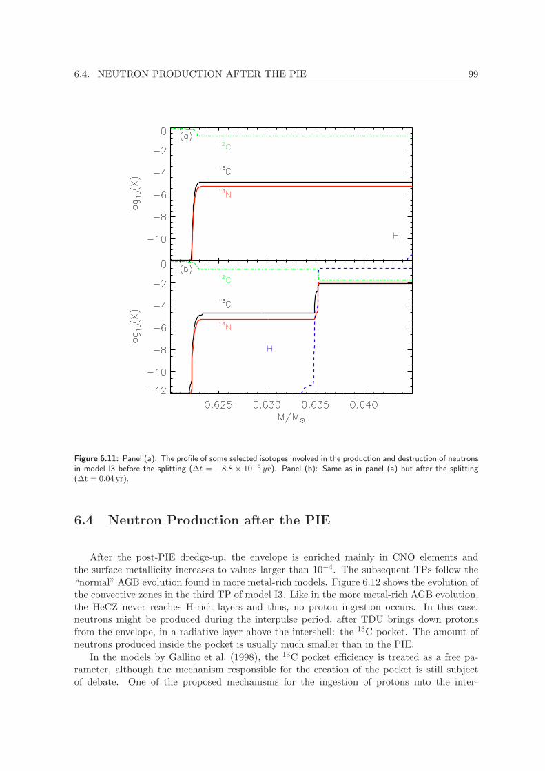
6.4. NEUTRON PRODUCTION AFTER THE PIE 99
Figure 6.11: Panel (a): The profile of some selected isotopes involved in the production and destruction of neutronsin model I3 before the splitting (∆t = −8.8 × 10⁻⁵ yr). Panel (b): Same as in panel (a) but after the splitting(∆t = 0.04 yr).
6.4 Neutron Production after the PIE
After the post-PIE dredge-up, the envelope is enriched mainly in CNO elements andthe surface metallicity increases to values larger than 10−4. The subsequent TPs follow the“normal” AGB evolution found in more metal-rich models. Figure 6.12 shows the evolution ofthe convective zones in the third TP of model I3. Like in the more metal-rich AGB evolution,the HeCZ never reaches H-rich layers and thus, no proton ingestion occurs. In this case,neutrons might be produced during the interpulse period, after TDU brings down protonsfrom the envelope, in a radiative layer above the intershell: the 13C pocket. The amount ofneutrons produced inside the pocket is usually much smaller than in the PIE.
In the models by Gallino et al. (1998), the 13C pocket efficiency is treated as a free pa-rameter, although the mechanism responsible for the creation of the pocket is still subjectof debate. One of the proposed mechanisms for the ingestion of protons into the inter-

100 CHAPTER 6. INTERMEDIATE-MASS STARS
Figure 6.12: The evolution of TP number three of model I3. There is no PIE in this TP. The HeCZ never reachesthe H-burning shell. Blue line is the position of maximum energy released by H-burning. Red line is the position ofmaximum energy released by He-burning. Time was shifted for clarity.
shell is the inclusion of diffusive overshooting at the lower border of the convective enve-lope (Herwig et al. 1997). We expect to find the 13C pocket in our models, since diffusiveovershooting is included. Also, at each TP another source of neutrons is expected to beactivated: the 22Ne(α, n)25Mg. During the TP, the intershell material is mixed and 14N isconverted into 22Ne through the reaction chain, 14N(α, γ)18F(β+ν)18O(α, γ)22Ne. The 22Neneutron source is activated for temperatures T ≥ 3.0× 10⁸K. In most metal-rich modelswith masses M < 4.0M⊙ this neutron source is only marginally activated (Iben & Truran1978; Straniero et al. 1997; Gallino et al. 1998). Figure 6.13 shows the maximum tempera-ture reached at the bottom of the HeCZ during the TP. All models reach after some TPs,the temperature of activation of the 22Ne neutron source. Our Tmax are in agreement withthe maximum temperatures found by Lugaro et al. (2012) when using the Stromlo evolutioncode for models M ≥ 2.0M⊙. However, it is important to keep in mind that the temperatureat the bottom of the HeCZ increases with the TP number and some models might achieveT = 3.0× 10⁸K at the very end of the TP evolution (see Figure 6.14). This implies that thisneutron source has differing degree of contribution to the s-process. The larger neutron fluxesresulting from the 22Ne source activate s-process branching that are usually not active in the13C pocket.
Neutrons can also be produced at the bottom of the HeCZ by the reaction 13C(α, n)16O,if enough 13C is left during the interpulse in the intershell. When the HeCZ is formed, 13C ismixed into high temperature regions and it is captured by 4He, releasing a large amount ofneutrons.
In the s-process calculations by Bisterzo et al. (2010) and Lugaro et al. (2012), the parametrizedefficiency of the 13C pocket is kept constant in all TPs. However, models by Cristallo et al.

6.4. NEUTRON PRODUCTION AFTER THE PIE 101
Figure 6.13: Maximum temperature at the bottom of the HeCZ during the TP as a function of the initial mass.
Figure 6.14: Temperature at the bottom of the HeCZ during the TP as a function of the TP number for model I1.
(2009b) performed with a code that have the s-process network coupled to the evolutionarycode, have shown that this is not the case. Instead, they have found that the efficiency ofthe pocket decreases with the TP number. Therefore, the first TPs should have the largest
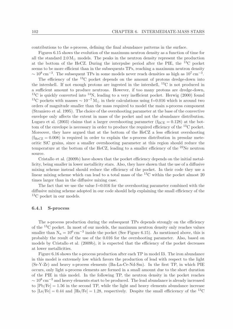
102 CHAPTER 6. INTERMEDIATE-MASS STARS
contributions to the s-process, defining the final abundance patterns in the surface.
Figures 6.15 shows the evolution of the maximum neutron density as a function of time forall the standard 2.0M⊙ models. The peaks in the neutron density represent the productionat the bottom of the HeCZ. During the interpulse period after the PIE, the 13C pocketseems to be more efficient than in the subsequents TPs, reaching a maximum neutron density∼ 108 cm−3. The subsequent TPs in some models never reach densities as high as 107 cm−3.
The efficiency of the 13C pocket depends on the amount of protons dredge-down intothe intershell. If not enough protons are ingested in the intershell, 13C is not produced ina sufficient amount to produce neutrons. However, if too many protons are dredge-down,13C is quickly converted into 14N, leading to a very inefficient pocket. Herwig (2000) found13C pockets with masses ∼ 10−7M⊙ in their calculations using f=0.016 which is around twoorders of magnitude smaller than the mass required to model the main s-process component(Straniero et al. 1995). The choice of the overshooting parameter at the base of the convectiveenvelope only affects the extent in mass of the pocket and not the abundance distribution.Lugaro et al. (2003) claims that a larger overshooting parameter (fBCE = 0.128) at the bot-tom of the envelope is necessary in order to produce the required efficiency of the 13C pocket.Moreover, they have argued that at the bottom of the HeCZ a less efficient overshooting(fHeCZ = 0.008) is required in order to explain the s-process distribution in presolar mete-oritic SiC grains, since a smaller overshooting parameter at this region should reduce thetemperature at the bottom of the HeCZ, leading to a smaller efficiency of the 22Ne neutronsource.
Cristallo et al. (2009b) have shown that the pocket efficiency depends on the initial metal-licity, being smaller in lower metallicity stars. Also, they have shown that the use of a diffusivemixing scheme instead should reduce the efficiency of the pocket. In their code they use alinear mixing scheme which can lead to a total mass of the 13C within the pocket almost 20times larger than in the diffusive mixing case.
The fact that we use the value f=0.016 for the overshooting parameter combined with thediffusive mixing scheme adopted in our code should help explaining the small efficiency of the13C pocket in our models.
6.4.1 S-process
The s-process production during the subsequent TPs depends strongly on the efficiencyof the 13C pocket. In most of our models, the maximum neutron density only reaches valuessmaller than Nn = 106 cm−3 inside the pocket (See Figure 6.15). As mentioned above, this isprobably the result of the use of the 0.016 for the overshooting parameter. Also, based onmodels by Cristallo et al. (2009b), it is expected that the efficiency of the pocket decreasesat lower metallicities.
Figure 6.16 shows the s-process production after each TP in model I3. The iron abundancein this model is extremely low which favors the production of lead with respect to the light(Sr-Y-Zr) and heavy s-process elements (Ba-La-Ce-Nd-Sm). In the first TP, in which PIEoccurs, only light s-process elements are formed in a small amount due to the short durationof the PIE in this model. In the following TP, the neutron density in the pocket reaches∼ 108 cm−3 and heavy elements start to be produced. The lead abundance is already increasedto [Pb/Fe] = 1.56 in the second TP, while the light and heavy elements abundance increaseto [Ls/Fe] = 0.44 and [Hs/Fe] = 1.28, respectively. Despite the small efficicency of the 13C

6.4. NEUTRON PRODUCTION AFTER THE PIE 103
Figure 6.15: Time evolution of the maximum neutron density for the 2.0M⊙ models.
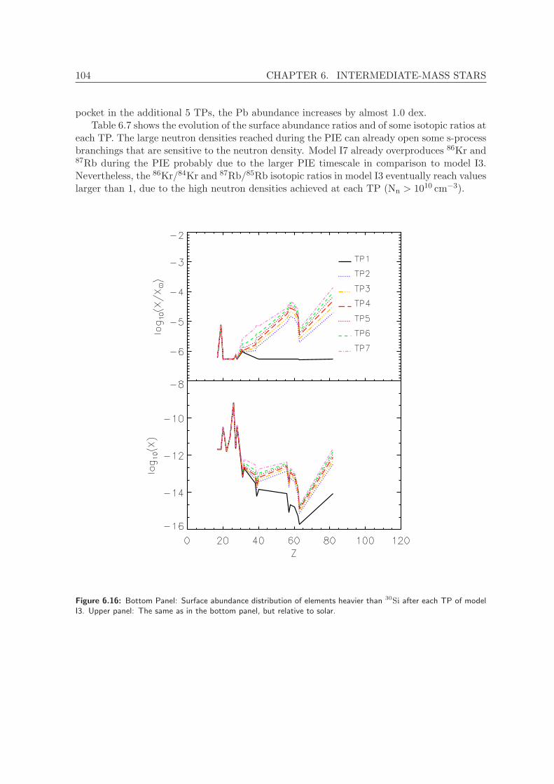
104 CHAPTER 6. INTERMEDIATE-MASS STARS
pocket in the additional 5 TPs, the Pb abundance increases by almost 1.0 dex.Table 6.7 shows the evolution of the surface abundance ratios and of some isotopic ratios at
each TP. The large neutron densities reached during the PIE can already open some s-processbranchings that are sensitive to the neutron density. Model I7 already overproduces 86Kr and87Rb during the PIE probably due to the larger PIE timescale in comparison to model I3.Nevertheless, the 86Kr/84Kr and 87Rb/85Rb isotopic ratios in model I3 eventually reach valueslarger than 1, due to the high neutron densities achieved at each TP (Nn > 1010 cm−3).
Figure 6.16: Bottom Panel: Surface abundance distribution of elements heavier than 30Si after each TP of modelI3. Upper panel: The same as in the bottom panel, but relative to solar.
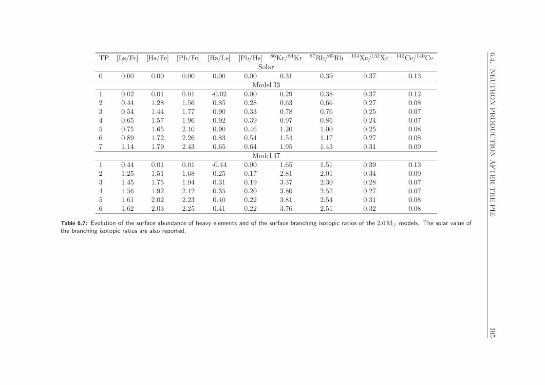
6.4.NEUTRON
PRODUCTIO
NAFTER
THE
PIE
105TP [Ls/Fe] [Hs/Fe] [Pb/Fe] [Hs/Ls] [Pb/Hs] 86Kr/84Kr 87Rb/85Rb 134Xe/132Xe 142Ce/140Ce
Solar
0 0.00 0.00 0.00 0.00 0.00 0.31 0.39 0.37 0.13
Model I3
1 0.02 0.01 0.01 -0.02 0.00 0.29 0.38 0.37 0.122 0.44 1.28 1.56 0.85 0.28 0.63 0.66 0.27 0.083 0.54 1.44 1.77 0.90 0.33 0.78 0.76 0.25 0.074 0.65 1.57 1.96 0.92 0.39 0.97 0.86 0.24 0.075 0.75 1.65 2.10 0.90 0.46 1.20 1.00 0.25 0.086 0.89 1.72 2.26 0.83 0.54 1.54 1.17 0.27 0.087 1.14 1.79 2.43 0.65 0.64 1.95 1.43 0.31 0.09
Model I7
1 0.44 0.01 0.01 -0.44 0.00 1.65 1.51 0.39 0.132 1.25 1.51 1.68 0.25 0.17 2.81 2.01 0.34 0.093 1.45 1.75 1.94 0.31 0.19 3.37 2.30 0.28 0.074 1.56 1.92 2.12 0.35 0.20 3.80 2.52 0.27 0.075 1.61 2.02 2.23 0.40 0.22 3.81 2.54 0.31 0.086 1.62 2.03 2.25 0.41 0.22 3.76 2.51 0.32 0.08
Table 6.7: Evolution of the surface abundance of heavy elements and of the surface branching isotopic ratios of the 2.0M⊙ models. The solar value ofthe branching isotopic ratios are also reported.

106 CHAPTER 6. INTERMEDIATE-MASS STARS
Variations in the mass of the 13C pocket can lead to significant changes in the s-process pre-dictions (Bisterzo et al. 2010; Lugaro et al. 2012). Bisterzo et al. (2010) treated the efficiencyof the 13C pocket as a free parameter in their calculations. This efficiency is varied in thecalculations with respect to their standard case (ST). The ST model with Z=0.01 reproducesthe solar system s-process abundances (Gallino et al. 1998). Predictions by Cristallo et al.(2009b) for [hs/ls] and [Pb/ls] are in good agreement with those of the ST case for high metal-licities. On the other hand, for lower metallicities the predictions for these two indices arein better agreement with models using smaller 13C pocket efficiencies. This can be explainedby the smaller efficiency found in their low Z models. The same was found by Lugaro et al.(2012) when comparing their prediction with these two studies. In this work, they varied themass of the proton mixing region. Models with smaller masses are in better agreement withpredictions by Cristallo et al. (2009b).
Bisterzo et al. (2010) have found that [ls/Fe] has a non linear behaviour with metallicity.Their ST model shows a local maximum at [Fe/H] ∼ −0.8. For metallicities smaller than[Fe/H] = −0.8, the s-process production shifts from the ls peak to the hs peak due to thereduction in the number of seeds, leading to a decrease in [ls/Fe]. In models with lowerpocket efficiencies they have found that the location of the maximum is shifted towards lowermetallicities due to the smaller amount of available neutrons. Finally, in their models, theyhave found a flat behaviour for metallicities [Fe/H] ≤ −2.0. Figure 6.17 shows our predictionsfor [ls/Fe] and [hs/Fe] in two 2.0M⊙ models. Our model with metallicity 10−7 (I7) showslarger [ls/Fe] than model I3. Model I7 have a more efficient PIE in which light elementswere produced due to its longer ∆PIE. Also, model I3 have less efficient 13C pockets in thesubsequent evolution as it can be seen in Figure 6.15.
The trend found by Bisterzo et al. (2010) for [hs/Fe] is similar to that of [ls/Fe]. Ourmodels I3 and I7 show similar [hs/Fe] values, although I7 presents slightly larger [hs/Fe]values due to larger 13C pocket efficiencies in this model.
Figure 6.18 shows our predictions for [hs/ls] and [Pb/hs] in two 2.0M⊙ models. Thepredictions from Cristallo et al. (2009b) for all their standard models and from Bisterzo et al.(2010) for models with metallicities [Fe/H] = −2.6 and [Fe/H] = −3.6 are also plotted. Thetwo conected symbols are the predictions for different pocket efficiencies. As it can be seen,they have found differences as large as 2.0 dex for the indices, depending on the efficiencyused. Our models present both [hs/ls] and [Pb/hs] smaller than 1.0 dex. This is in agreementwith the lower metallicity models calculated by Bisterzo et al. (2010) using efficiencies smallerthan ST/12.
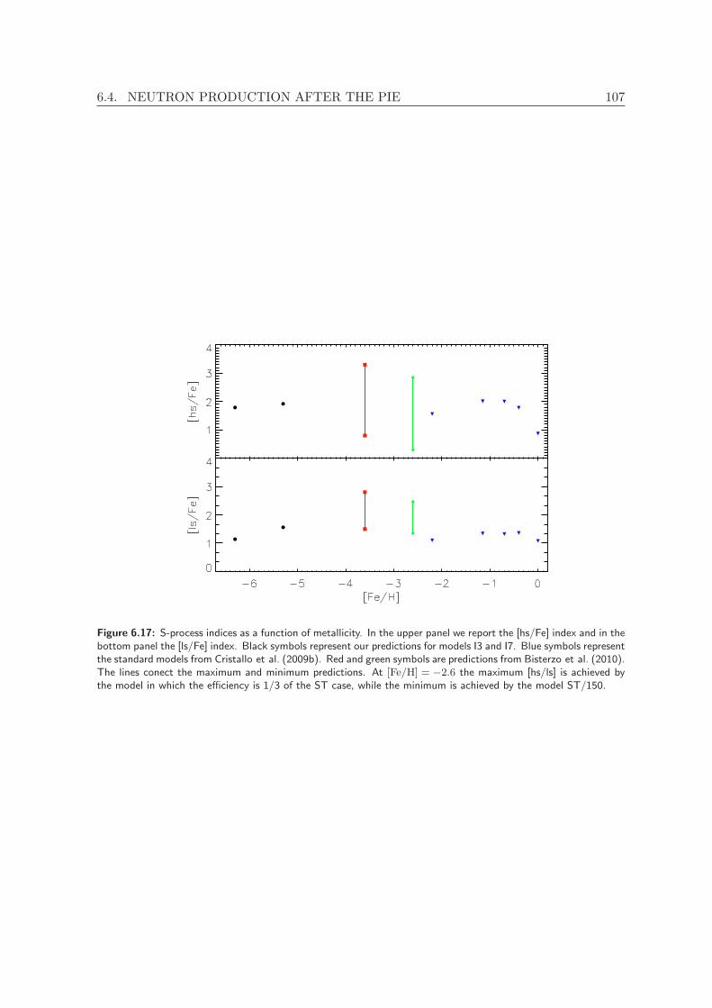
6.4. NEUTRON PRODUCTION AFTER THE PIE 107
Figure 6.17: S-process indices as a function of metallicity. In the upper panel we report the [hs/Fe] index and in thebottom panel the [ls/Fe] index. Black symbols represent our predictions for models I3 and I7. Blue symbols representthe standard models from Cristallo et al. (2009b). Red and green symbols are predictions from Bisterzo et al. (2010).The lines conect the maximum and minimum predictions. At [Fe/H] = −2.6 the maximum [hs/ls] is achieved bythe model in which the efficiency is 1/3 of the ST case, while the minimum is achieved by the model ST/150.

108 CHAPTER 6. INTERMEDIATE-MASS STARS
Figure 6.18: S-process indices as a function of metallicity. In the upper panel we report the [Pb/hs] index and in thebottom panel the [hs/ls] index. Black symbols represent our predictions for models I3 and I7. Blue symbols representthe standard models from Cristallo et al. (2009b). Red and green symbols are predictions from Bisterzo et al. (2010).The lines conect the maximum and minimum predictions. At [Fe/H] = −2.6 the maximum [hs/ls] is achieved bythe model in which the efficiency is 1/3 of the ST case, while the minimum is achieved by the model ST/150.

6.5. LIGHT ELEMENTS 109
6.5 Light elements
The post-PIE dredge-up brings to the surface products of the nucleosynthesis during thePIE and of the nucleosynthesis after the splitting of the convective zone (happening in theHCZ). Figure 6.19 shows the surface abundance evolution of light elements (A < 30) for the2.0M⊙ model with zero metallicity. The first abrupt increase in the abundances indicatesthe post-PIE dredge-up. Isotopes involved in the CNO cycles are the main product of thisphenomenon. We have found that the most abundant isotope after the post-PIE dredge-up is 12C, followed by 14N. Nonetheless, for a model with the same mass and metallicity,Campbell (2007) have found that 16O is the main product of the PIE (see their Figure 6.24).This difference might be explained by the inclusion of overshooting in our models. More 12Cfrom the core is brought to the HeCZ in the overshooting model, which should explain itsdominance. Moreover, the inclusion of overshooting results in a faster splitting of the HeCZ,as it was shown in Chapter 5, which should slow the 16O production through 13C(α, n)16Oand 12C(α, γ)16O. Further in the AGB evolution, the 12C abundance continues to increasedue to TDU, while the 14N remains the same, resulting in an increase in the C/N ratio. Thesame happens with the 12C/13C ratio (Figure 6.19). This is in contrast with Campbell (2007)results. They found HBB in their model which converted 12C into 14N, decreasing the C/Nratio. HBB is not found in our model, since the temperature at the bottom of the convectiveenvelope remains lower than 2× 10⁷K during the entire TP-AGB. It is important to stressthat the mass boundary for the occurrence of HBB strongly varies between studies. WhilstCampbell (2007) and Siess et al. (2002) found HBB in zero metallicity models with massesdown to M = 2.0M⊙, Lau et al. (2009) and Suda & Fujimoto (2010) did not find HBB forsuch low-mass stars.
The abundance of fluorine is enhanced during the PIE and continues to increase through-out the AGB. Ashes from the H-burning (13C and 14N) are mixed down in the intershellwhen a new TP occurrs and a new HeCZ is formed. 13C is captured by the abundant4He and neutrons are produced. The released neutrons are captured by 14N, producingprotons through the reaction 14N(n, p)14C. At the same time fluorine is formed via the re-action chain 18O(p, α)15N(α, γ)19F with 18O being provided by the 14N(α, γ)18F(β+ν)18Ochain. Fluorine is then transported to the surface during TDU. Among the isotopes in-volved in the NeNa chain, 22Ne is the most abundant during the PIE, due to the chain14N(α, γ)18F(β+ν)18O(α, γ)22Ne. It continues to be produced during the subsequents TPsdue to the mixing of 14N-rich layers into the newly formed HeCZ as explained above for thefluorine case. Since HBB does not happen in this model, 22Ne is not destroyed in the envelope,in contrast to Campbell (2007) results.
Another element that is largely produced during the PIE is lithium. As explained in Chap-ter 5, the high temperature at the HCZ activate the reaction 3He(α, γ)7Be, producing 7Bewhich in turn decays to produce 7Li. In all our model with M ≤ 2.0M⊙ lithium is producedduring the PIE in a large amount and it is preserved during the subsequent evolution, sincethe temperature at the bottom of the envelope is not high enough to activate the 7Li(p, α)4Hereaction (T ∼ 2.5× 10⁶K). This is in agreement with Iwamoto et al. (2004) results for starswith M ≤ 2.0M⊙ and metallicity [Fe/H] = −2.7. Nevertheless, models with 3.0M⊙ reachtemperatures larger than 2.5× 10⁶K at the bottom of the HeCZ, leading to lithium depletionin the subsequent TPs.
Figures 6.20 and 6.21 show a comparison between our yields and those by Campbell (2007)
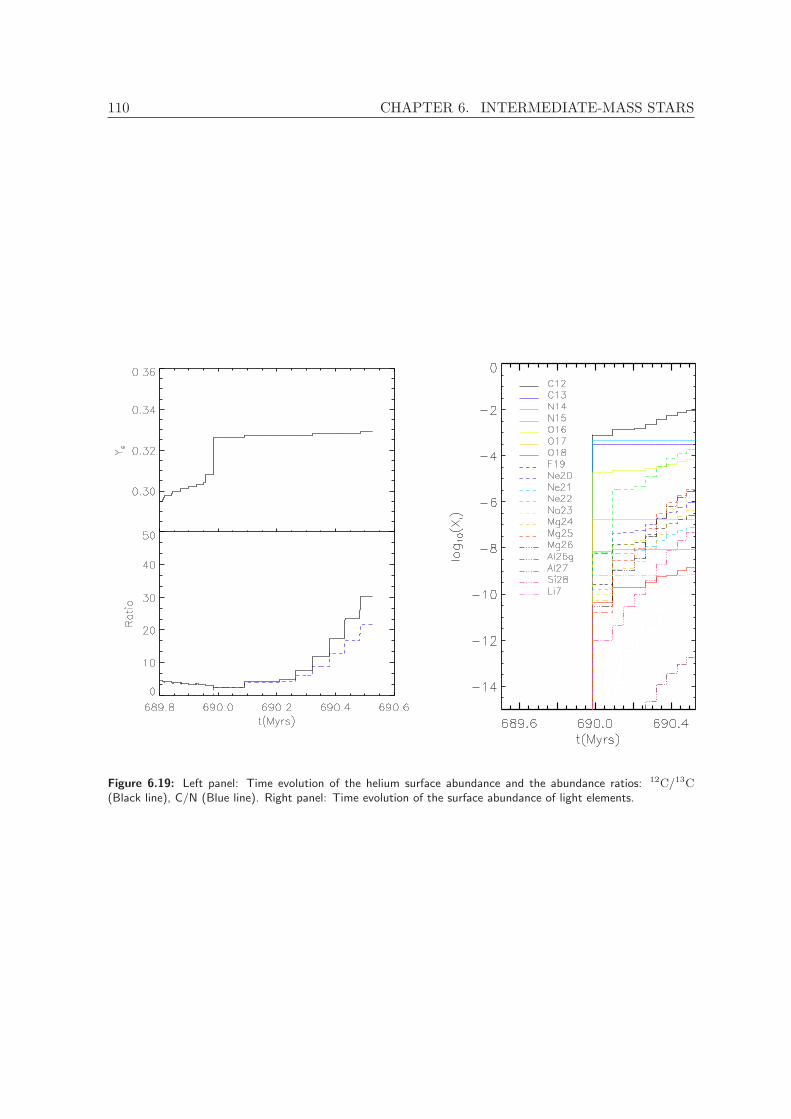
110 CHAPTER 6. INTERMEDIATE-MASS STARS
Figure 6.19: Left panel: Time evolution of the helium surface abundance and the abundance ratios: 12C/13C(Black line), C/N (Blue line). Right panel: Time evolution of the surface abundance of light elements.

6.5. LIGHT ELEMENTS 111
for the zero metallicity models. It can be seen that the yields from Campbell (2007) modelspresent strong HBB signatures. Whilst our models overproduce carbon with respect to theSun, their models converted the carbon dredge-up after the PIE and in the first TDUs into14N. The same effect can be seen in the fluorine to magnesium isotopes. HBB predictionsdepend on, for instance, the adopted mass-loss rate. Campbell (2007) models have smallermass-loss rates and undergo much more TPs than our models. The larger mass-loss rate inour models induces a faster cooling of the stellar structure, decreasing the chances of HBB tooccur.
Figure 6.20: Elemental yields for our zero metallicity models against initial stellar mass. Blue squares representthe yields from Campbell (2007) and black circles represent our values. The solar abundance used on both yields isfrom Grevesse & Sauval (1998).
Except for lithium and nitrogen, the yields of all light elements increase with increasingmass. The lithium abundance after the PIE depends on the maximum temperature at thebotttom of the HCZ, right after the splitting, and on the time between the splitting and thedredge-up ∆td. The amount of nitrogen depends mostly on ∆td. The longer it takes for theenvelope to start dredging-up material from the HCZ, the larger the abundance of 14N. The3.0M⊙ model has ∆td smaller than the 2.0M⊙ model which should explain the differences in14N abundance.
Figures 6.22 and 6.23 show the yields of all 2.0M⊙ models. In our models, the lithiumabundance increases with metalliticy, while in models by Campbell (2007) they decrease withmetallicity. This is probably due to the fact that in their model with [Fe/H] = −3.0, PIEdoes not occur and lithium is produced only through HBB. The larger lithium abundancein our Z = 10−5 model could be explained by the smaller ∆td in this model. Therefore, 7Li

112 CHAPTER 6. INTERMEDIATE-MASS STARS
Figure 6.21: Elemental yields for our zero metallicity models against initial stellar mass. Blue squares represent theyields from Campbell (2007) and black circles represent our values.
is quickly carried to low temperature regions in this model where it cannot be destroyed byproton captures. On the other hand, the carbon yields are almost constant in this metallicityrange. It is clear from these plots that all Campbell (2007) models show HBB signatures: largenitrogen content, small carbon abundance, large sodium abundance and small fluorine andneon abundances. Nevertheless, our models do not undergo HBB at any initial metallicity.
The 4He abundance is dominated by the second the post-PIE dredge-ups since HBB doesnot occur in our models. Table 6.8 shows the final 4He surface abundance. The SDU increasethe initial abundance, Y0
s = 0.245, in 8-45%. PIE, on the other hand, increases the heliumabundance in about 10%. Finally, the final abundance is increased by less than 1% in thesubsequent TPs.
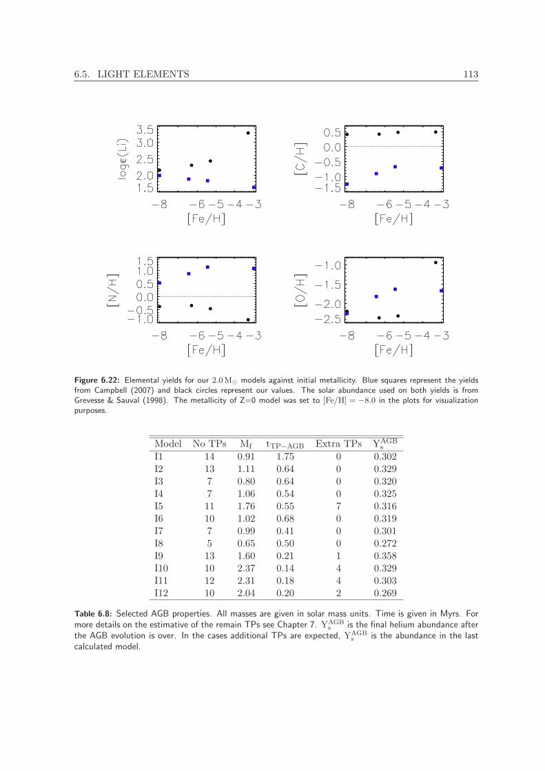
6.5. LIGHT ELEMENTS 113
Figure 6.22: Elemental yields for our 2.0M⊙ models against initial metallicity. Blue squares represent the yieldsfrom Campbell (2007) and black circles represent our values. The solar abundance used on both yields is fromGrevesse & Sauval (1998). The metallicity of Z=0 model was set to [Fe/H] = −8.0 in the plots for visualizationpurposes.
Model No TPs Mf tTP−AGB Extra TPs YAGBs
I1 14 0.91 1.75 0 0.302I2 13 1.11 0.64 0 0.329I3 7 0.80 0.64 0 0.320I4 7 1.06 0.54 0 0.325I5 11 1.76 0.55 7 0.316I6 10 1.02 0.68 0 0.319I7 7 0.99 0.41 0 0.301I8 5 0.65 0.50 0 0.272I9 13 1.60 0.21 1 0.358I10 10 2.37 0.14 4 0.329I11 12 2.31 0.18 4 0.303I12 10 2.04 0.20 2 0.269
Table 6.8: Selected AGB properties. All masses are given in solar mass units. Time is given in Myrs. Formore details on the estimative of the remain TPs see Chapter 7. YAGB
s is the final helium abundance afterthe AGB evolution is over. In the cases additional TPs are expected, YAGB
s is the abundance in the lastcalculated model.
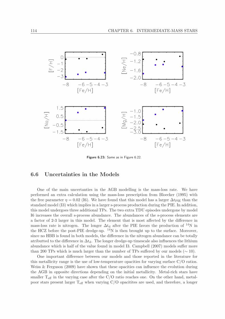
114 CHAPTER 6. INTERMEDIATE-MASS STARS
Figure 6.23: Same as in Figure 6.22.
6.6 Uncertainties in the Models
One of the main uncertanties in the AGB modelling is the mass-loss rate. We haveperformed an extra calculation using the mass-loss prescription from Bloecker (1995) withthe free parameter η = 0.02 (I6). We have found that this model has a larger ∆tPIE than thestandard model (I3) which implies in a larger s-process production during the PIE. In addition,this model undergoes three additional TPs. The two extra TDU episodes undergone by modelI6 increases the overall s-process abundance. The abundances of the s-process elements area factor of 2-3 larger in this model. The element that is most affected by the difference inmass-loss rate is nitrogen. The longer ∆td after the PIE favors the production of 14N inthe HCZ before the post-PIE dredge-up. 14N is then brought up to the surface. Moreover,since no HBB is found in both models, the difference in the nitrogen abundance can be totallyatributted to the difference in ∆td. The longer dredge-up timescale also influences the lithiumabundance which is half of the value found in model I3. Campbell (2007) models suffer morethan 200 TPs which is much larger than the number of TPs suffered by our models (∼ 10).
One important difference between our models and those reported in the literature forthis metallicity range is the use of low-temperature opacities for varying surface C/O ratios.Weiss & Ferguson (2009) have shown that these opacities can influence the evolution duringthe AGB in opposite directions depending on the initial metallicity. Metal-rich stars havesmaller Teff in the varying case after the C/O ratio reaches one. On the other hand, metal-poor stars present larger Teff when varying C/O opacitites are used, and therefore, a longer
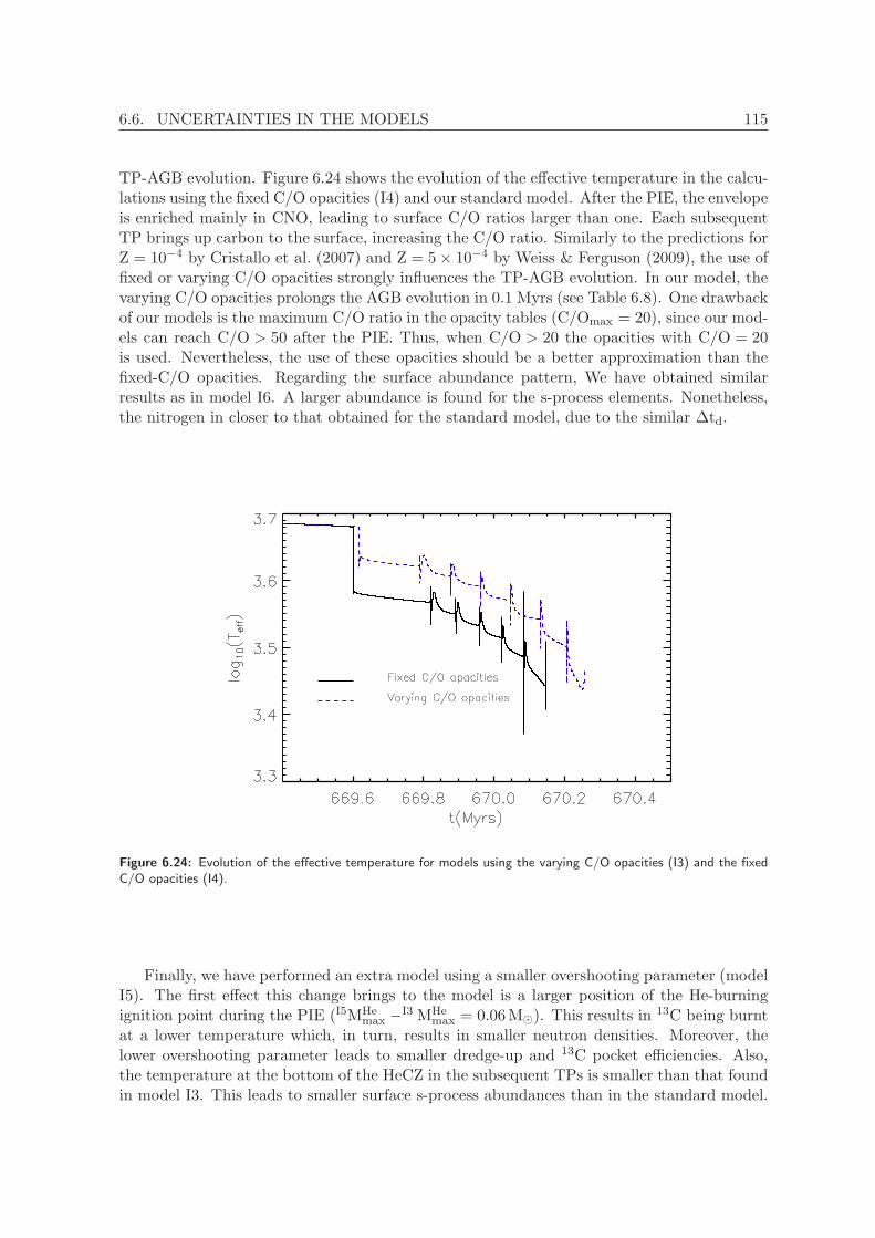
6.6. UNCERTAINTIES IN THE MODELS 115
TP-AGB evolution. Figure 6.24 shows the evolution of the effective temperature in the calcu-lations using the fixed C/O opacities (I4) and our standard model. After the PIE, the envelopeis enriched mainly in CNO, leading to surface C/O ratios larger than one. Each subsequentTP brings up carbon to the surface, increasing the C/O ratio. Similarly to the predictions forZ = 10−4 by Cristallo et al. (2007) and Z = 5× 10⁻⁴ by Weiss & Ferguson (2009), the use offixed or varying C/O opacities strongly influences the TP-AGB evolution. In our model, thevarying C/O opacities prolongs the AGB evolution in 0.1 Myrs (see Table 6.8). One drawbackof our models is the maximum C/O ratio in the opacity tables (C/Omax = 20), since our mod-els can reach C/O > 50 after the PIE. Thus, when C/O > 20 the opacities with C/O = 20is used. Nevertheless, the use of these opacities should be a better approximation than thefixed-C/O opacities. Regarding the surface abundance pattern, We have obtained similarresults as in model I6. A larger abundance is found for the s-process elements. Nonetheless,the nitrogen in closer to that obtained for the standard model, due to the similar ∆td.
Figure 6.24: Evolution of the effective temperature for models using the varying C/O opacities (I3) and the fixedC/O opacities (I4).
Finally, we have performed an extra model using a smaller overshooting parameter (modelI5). The first effect this change brings to the model is a larger position of the He-burningignition point during the PIE (I5MHe
max −I3 MHe
max = 0.06M⊙). This results in13C being burnt
at a lower temperature which, in turn, results in smaller neutron densities. Moreover, thelower overshooting parameter leads to smaller dredge-up and 13C pocket efficiencies. Also,the temperature at the bottom of the HeCZ in the subsequent TPs is smaller than that foundin model I3. This leads to smaller surface s-process abundances than in the standard model.
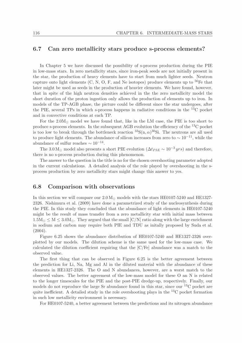
116 CHAPTER 6. INTERMEDIATE-MASS STARS
6.7 Can zero metallicity stars produce s-process elements?
In Chapter 5 we have discussed the possibility of s-process production during the PIEin low-mass stars. In zero metallicity stars, since iron-peak seeds are not initially present inthe star, the production of heavy elements have to start from much lighter seeds. Neutroncapture onto light elements (C, N, O, F, and Ne isotopes) produce elements up to 56Fe thatlater might be used as seeds in the production of heavier elements. We have found, however,that in spite of the high neutron densities achieved in the the zero metallicity model theshort duration of the proton ingestion only allows the production of elements up to iron. Inmodels of the TP-AGB phase, the picture could be different since the star undergoes, afterthe PIE, several TPs in which s-process happens in radiative conditions in the 13C pocketand in convective conditions at each TP.
For the 2.0M⊙ model we have found that, like in the LM case, the PIE is too short toproduce s-process elements. In the subsequent AGB evolution the efficiency of the 13C pocketis too low to break through the bottleneck reaction 33S(n, α)30Si. The neutrons are all usedto produce light elements. The abundance of silicon increases from zero to ∼ 10−11, while theabundance of sulfur reaches ∼ 10−14.
The 3.0M⊙ model also presents a short PIE evolution (∆tPIE ∼ 10−3 yrs) and therefore,there is no s-process production during this phenomenon.
The answer to the question in the title is no for the chosen overshooting parameter adoptedin the current calculations. A detailed analysis of the role played by overshooting in the s-process production by zero metallicity stars might change this answer to yes.
6.8 Comparison with observations
In this section we will compare our 2.0M⊙ models with the stars HE0107-5240 and HE1327-2326. Nishimura et al. (2009) have done a parametrized study of the nucleosynthesis duringthe PIE. In this study they concluded that the abundance of light elements in HE0107-5240might be the result of mass transfer from a zero metallicity star with initial mass between1.5M⊙ ≤ M ≤ 3.0M⊙. They argued that the small [C/N] ratio along with the large enrichmentin sodium and carbon may require both PIE and TDU as initally proposed by Suda et al.(2004).
Figure 6.25 shows the abundance distribution of HE0107-5240 and HE1327-2326 over-plotted by our models. The dilution scheme is the same used for the low-mass case. Wecalculated the dilution coefficient requiring that the [C/Fe] abundance was a match to theobserved value.
The first thing that can be observed in Figure 6.25 is the better agreement betweenthe prediction for Li, Na, Mg and Al in the diluted material with the abundance of theseelements in HE1327-2326. The O and N abundances, however, are a worst match to theobserved values. The better agreement of the low-mass model for these O an N is relatedto the longer timescales for the PIE and the post-PIE dredge-up, respectively. Finally, ourmodels do not reproduce the large Sr abundance found in this star, since our 13C pocket arequite inefficient. A detailed study in the role overshooting plays in the 13C pocket formationin such low metallicity environment is necessary.
For HE0107-5240, a better agreement between the predictions and its nitrogen abundance
6.9. SUMMARY 117
Figure 6.25: Comparison between the abundance distribution of HE0107-5240 (blue symbols - upper panel) andHE1327-2326 (red symbols 0 bottom panel) and our AGB models. Upper panel: The black dotted line indicatesthe final surface abundance after the last TDU of model I7. The blue line indicates the average abundance lost bythe star diluted in the observed star material (I7). The orange line represents the diluted model M2 from Chapter5. Bottom panel: The black dashed line indicates the final surface abundance after the last TDU of model I3. Thered line indicates the average abundance lost by the star diluted in the observed star material (I3). The green linerepresents the diluted model M2 from Chapter 5.
is found for the 2.0M⊙ model. Nevertheless, the shorter PIE results in a worst agreementfor the oxygen abundance. Moreover, intermediate elements (Mg, Al, Ca, Ti, Ni) are alsoin better agreement with the 2.0M⊙ model. For the s-process elements, the changes are notsignificant and this model is also able to reproduce the abundances within a factor of 4. Itseems from our models that the suggestion by Nishimura et al. (2009) in which the primarystar has a mass between 1.5M⊙ ≤ M ≤ 3.0M⊙ is the most favorable scenario. However, it isimportant to keep in mind that the large uncertainties regarding the modelling of the PIEmust be studied in detail and low-mass stars cannot be discarded as a possible companion forHE0107-5240.
6.9 Summary
We have performed evolutionary and nucleosynthesis calculations of intermediate-mass EMPand zero metallicity stars. All our models undergo PIE. For masses M ≤ 2.0M⊙ we find a goodagreement in the metallicity boundary for the occurrence of the PIE with the results fromCampbell (2007) and Suda & Fujimoto (2010). For the 3.0M⊙ models large discrepancies arefound between other literature studies and our models.
We have explored the nucleosynthesis of light and heavy elements in these stars, speciallyduring the PIE. The nucleosynthesis during the PIE is strongly influenced by the duration ofthis phenomenon (∆tPIE). Our models present a variety of values of ∆tPIE: from ∼ 10−4 up

118 CHAPTER 6. INTERMEDIATE-MASS STARS
to ∼ 7× 10⁻¹ yrs. Amongst the models with Z = 10−8, the 3.0M⊙ model shows a significants-process production during PIE, while in models with Z = 10−7 only light s-process elementsare formed during the PIE. The 2.0M⊙ model with the highest metallicity presents the largers-process production during the PIE, due to the large ∆tPIE.
For the nucleosynthesis post-PIE, our models confirm the trend found by Cristallo et al.(2009b) that the 13C pocket efficiency should decrease with metallicity. However, it is impor-tant to stress that the overshooting parameter plays a major role in the 13C pocket efficiency.Furthermore, the overshooting parameter also plays a role in the convective s-process. Thelarge the overshooting parameter, the smaller is the He-burning ignition point during the PIEand at each new TP. We have also found that the interpulse period following the PIE havethe stronger contribution to the s-process production.
Concerning the light elements, the evolution post-PIE is also of utmost importance forthe final yields. Comparison between our yields and those by Campbell (2007) have shownthat they can be extremely different. This difference is the result of the occurrence of HBBin their models. Our models do not undergo HBB, resulting in carbon enriched stars.
We have discussed the influence of the main uncertainties in the final abundances. Themass-loss rate by Bloecker (1995) does not alter the AGB evolution by a large fraction.However, the extra TDU episodes increases the s-process abundance by a factor of 2 to 4.The same can be discussed about the use of fixed C/O opacities instead of those with varyingC/O. For the low metallicity range studied the varying C/O opacities tend to prolong theAGB evolution. In this particular model the use of fixed C/O opacities resulted in ∆tPIE and∆td approximately two orders of magnitude larger and one order of magnitude smaller thanin model I3, respectively .
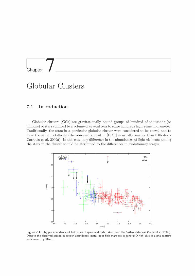
Chapter 7Globular Clusters
7.1 Introduction
Globular clusters (GCs) are gravitationally bound groups of hundred of thousands (ormillions) of stars confined to a volume of several tens to some hundreds light years in diameter.Traditionally, the stars in a particular globular cluster were considered to be coeval and tohave the same metallicity (the observed spread in [Fe/H] is usually smaller than 0.05 dex -Carretta et al. 2009a). In this case, any difference in the abundances of light elements amongthe stars in the cluster should be attributed to the differences in evolutionary stages.
-0.5
0.0
0.5
1.0
1.5
2.0
2.5
-4.5 -4.0 -3.5 -3.0 -2.5 -2.0 -1.5 -1.0 -0.5 0.0
[O/F
e]
[Fe/H]
295
-0.546
295
-0.546
MPEMP,RGBEMP,MS
Figure 7.1: Oxygen abundance of field stars. Figure and data taken from the SAGA database (Suda et al. 2008).Despite the observed spread in oxygen abundance, metal-poor field stars are in general O-rich, due to alpha captureenrichment by SNe II.

120 CHAPTER 7. GLOBULAR CLUSTERS
Observations of field stars have shown that stars with metallicities [Fe/H] ≤ −1.0 exhibitan overabundance of alpha capture elements (O, Ne, Mg, Si, Ca, Ti) in comparison to theiron abundance ([α/Fe] ∼ 0.4 - See Figure 7.1). Alpha capture elements are mainly producedby massive stars (M > 10M⊙) when they end their lives as core-collapse type II supernovae(SNe II). Iron, on the other hand, is mainly produced by Type Ia supernovae (SNe Ia). Theoccurrence of SNe II and SNe Ia have quite different timescales. While SNe II occur withint ≤ 107 yrs, SNe Ia have mean lifetimes larger than t ∼ 1Gyr. Therefore, the insterstellarmedium contamination by SNe Ia occurs much later, reducing the abundance ratio [α/Fe] (at[Fe/H] ∼ −1.0).
GCs are old objectcs (age > 10Gyrs) with metallicities −2.3 < [Fe/H] < 0.0. The abun-dances of light elements of individual stars in the cluster were expected to reflect the yieldsof SNe II and the internal changes due to their evolutionary stages. For instance, GC starsin the upper RGB were expected to have smaller 12C/13C ratios, due to the first dredge-up,than the ratios present in the MS stars. On the other hand, they were expected to be O-richand Na-poor at any evolutionary stage preceding the AGB. Nevertheless, early investigationshave shown that stars in GCs present abundance patterns that cannot be explained only bythe expected surface abundance changes due to stellar evolution (Kraft 1994). More recentspectroscopic analysis of stars in GC have confirmed the existence of star-to-star abundancevariations (Gratton et al. 2001; Ramırez & Cohen 2002; Carretta et al. 2004, 2009c,b). Thesevariations, usually found to be anticorrelated: O-Na and Mg-Al anticorrelations, are not foundin field stars (Gratton et al. 2000).
Figure 7.2: O-Na anticorrelation in NGC 6752. Black filled circles are measurements from Carretta et al. 2007.Green symbols are from Grundahl et al. 2002. The line indicate the separation between primordial and secondgeneration as suggested by Carretta et al. 2009c.
Figure 7.2 shows the O-Na anticorrelation for NGC 6752. The stars below the horizontalline have oxygen and sodium abundances similar to those found in field stars with the same

7.1. INTRODUCTION 121
metallicity ([Fe/H] ∼ −1.5). As explained in Chapter 2, during the star ascension in the HRdiagram, the envelope deepens down and products of H-burning are brought up to the stellarsurface (FDU). However, standard evolutionary calculations of low-mass stars have shownthat the changes in surface abundance due to FDU are very modest. The envelope does notreach deep enough regions where p-capture reactions might produce N from O (ON-cycle)and 23Na from 22Ne, in order to explain the O-poor and Na-rich stars observed above thehorizontal line in Figure 7.2
Figure 7.3: The color-magnitude digram of M3. Credit: http://www.astro.ljmu.ac.uk.
Since the general idea was that stars in GC belong to a single stellar population1 it wasnatural to investigate if some non-canonical extra mixing during the RGB phase could explainthe observed abundance anomalies (Denissenkov & Weiss 2001). Denissenkov & Weiss 1996have explored the possibility that additional mixing in a region between the H-burning shell(HBS) and the bottom of the convective envelope (BCE) would explain the observed O-Naanticorrelation in GCs, the so called “deep mixing scenario”. They were able to reproduce theO-Na anticorrelation for the giants in the clusters M92 and M13. Nonetheless, the discoveryof anomalous abundances also in unevolved stars (Gratton et al. 2001) indicates that thesurface abundance patterns were already present when these stars were formed.
Early photometric analysis of GC had also led to the believe that one single stellar pop-ulation, i. e. one isochrone2, could fit the color-magnitude diagram (CMD) of a globularcluster (Figure 7.3). Only the high quality photometry achieved in the last few years hasbeen able to reveal that GC can present multiple main sequences and subgiant branchs inthe CMD (Piotto et al. 2007; Piotto 2009): a clear evidence of multiple populations. Figure7.4 shows the multiple main sequences found in the cluster NGC 2808 (Piotto et al. 2007).The different MSs in this cluster can be explained by different stellar populations, present-ing different helium contents (see inner plot in Figure 7.4), since the spread in metallicity isnot large enough to account for the presence of different MSs in the HRD. The high heliumabundance of the bluest MS (Y ∼ 0.38) can be explained by an ealier pollution of the cloudin which these stars were formed, since MS low-mass stars do not have a convective envelopeable to transport H-burning material to the surface.
The abundance variations in GCs are expected to be reflected in the CMDs. Sbordone et al.
1Single stellar population is a group of stars, with different masses, having the same initial composition and

122 CHAPTER 7. GLOBULAR CLUSTERS
Figure 7.4: The color-magnitude diagram of NGC 2808. Taken from Piotto et al. 2007. The inner plot shows thesuperposition to the CMD of isochrones with different initial helium abundance.
2011 have performed theoretical calculations of the effect these variations have in the CMDs.They have found that different compositions affect the CMD in different ways. Moreover,depending on the filter used the effects can be large or negligible. For instance, they haveshown that in the CMDs using the filters BVI, only a change in helium abundance wouldcause a splitting in the MS, while a variation of the C+N+O abundance should lead to asplit in the SGB. This could help explaining, for instance, the empirical splitting in the SGBfound for NGC 1851.
Finally, in the framework of multiple stellar populations, the horizontal branch (HB)morphology could also be explained by differing He abundances. Stars in the bluer HBshould have a Helium abundance larger than those in the red HB (D’Antona et al. 2002;D’Antona & Caloi 2004).
In the light of the spectroscopic and photometric results discussed above, one possiblescenario invokes the existence of at least two stellar populations in GCs. The more massivestars in the first stellar generation polluted the intra-cluster medium, via stellar winds, wherelater, a second generation of stars was formed. The nature of the polluting stars from the firstgeneration is not yet established: they could be either massive AGB stars (Ventura et al. 2001)or rapidly rotating massive stars (Decressin et al. 2007). Massive AGB stars undergo hotbottom-burning (HBB - see Chapter 2 for more details) which is responsible for converting 12Cinto 14N. Furthermore, the high temperatures at the bottom of convective envelope activate
age.2Lines in the HR diagram occupied by stars of different masses but the same age.

7.2. THE MODELS 123
more advanced proton capture reactions: the NeNa and MgAl chains that, in principle, couldaccount for the O-Na and Mg-Al anticorrelations.
Ventura et al. (2001) have performed the first full AGB calculations for intermediate-massstars with metallicities compatible with the observed GCs. No quantitative results regardingthe anticorrelations could be obtained due to the small network used in the calculations.However, they have found a strong depletion of 16O in their models, which was an indicationthat advanced nucleosynthesis was occurring, and therefore producing Na and Al throughproton capture. Fenner et al. (2004) have performed AGB calculations of stars with massesM < 7.0M⊙ and metallicities [Fe/H] < −1.4. In this study, they have used a nuclear networkincluding all elements involved in the advanced proton capture chains. Their models were ableto reproduce the observed spread in Na and Al. However, neither O or Mg were sufficientlydepleted in their models in order to match the observed O-Na and Mg-Al anticorrelationsin GCs. In addition, the sum C+N+O did not remain constant in their models contrary towhat is found for many GCs (Ivans et al. 1999). Denissenkov & Herwig (2003) models werealso not able to reproduce the observed GCs patterns. They have found that the temperatureat the base of the convective envelope necessary to deplete oxygen, leads to 25Mg/24Mg and26Mg/24Mg ratios larger than the observed.
Denissenkov & Herwig (2003) and Fenner et al. (2004) claimed that it is unlikely thatAGB stars are the polluters responsible for the abundance pattern observed in stars of thesecond generation. However, Ventura and collaborators argued that the use of a more effi-cienty convection theory in their models produces results more consistent with the observa-tions. It is important to point it out that since 2004 mostly Ventura and collaborators havebeen publishing on the subject, while little work has been done by other groups. We havetaken advantage of the newest GARSTEC nuclear network, including advanced H-burning,and have performed models of intermediate-mass stars with metallicities close to the observedGC. We have used the most up-to-date reaction rates, specially those involved in the advancedH-burning (Iliadis et al. 2010) and the low-temperature opacities for varying C/O-ratios.
7.2 The Models
We have performed evolutionary calculations from the ZAMS to the TP-AGB phase forstars with metallicities Z=0.001 and Z=0.004 and masses 3.0 ≤ M/M⊙ ≤ 5.0. The initialcomposition is alpha-enhanced, which means that the abundances of O, Ne, Mg, and Si areenhanced by 0.4 dex. The physical inputs used in the models are the same as those usedin Chapter 6 (Models G1-G6). Extra models using the mass-loss prescription by Bloecker(1995) and without overshooting have been performed (Models G7-G9). Table 7.1 shows themodels and some selected AGB properties. In the second column the initial zero-age MainSequence mass is given (MZAMS). The third column contains the initial metallicity (Z). Thefourth and fifth columns give the total number of TPs experienced by the model (No TPs)and the final total mass (Mf), respectively. Further in this Chapter, we will estimate theamount of remaining TPs, not computed due to convergence problems. The number of TPsactually simulated and the final total mass, in Table 7.1, will give us an idea of how muchfurther in the evolution we were able to simulate.

124 CHAPTER 7. GLOBULAR CLUSTERS
Model MZAMS Z No TPs Mf
G1 3.0 0.001 13 1.59G2 4.0 0.001 20 2.74G3 5.0 0.001 63 3.67G4 3.0 0.004 10 1.26G5 4.0 0.004 18 3.20G6 5.0 0.004 51 3.39G7 5.0 0.001 57 1.60G8 3.0 0.001 24 0.86G9 4.0 0.001 38 1.58
Table 7.1: List of computed models and selected AGB properties. All masses are given in solar mass units.
7.3 Results
Intermediate-mass stars undergo the so-called HBB phenomenon. During the AGB, thebottom of the convective envelope can reach high temperatures: Tbce = (0.5− 1.0)× 108K.These high temperatures activate advanced H-burning in this region, leading to the surfacedepletion of carbon and oxygen and the enrichment of nitrogen. Figure 7.5 shows the tem-perature at the bottom of the convective envelope along the AGB evolution for our standardmodels. Our 3.0M⊙ models (black lines in Figure 7.5) present mild temperatures, whichshould imply in a negligible contribution from HBB to the abundance patterns in these stars.This can be seen in Figure 7.6 by the surface time evolution of carbon and nitrogen. IfHBB was operating efficiently in this model, 12C should be converted into 14N. Instead, 12Cabundance increases at each TP due to the dredge-up of intershell material. 22Ne and theMg isotopes are also enhanced by TDU. 22Ne is synthesised via α captures in the convectiveshell during the TP. It is, then, partially converted to 23Na after the dredge-up, increasingthe surface 23Na abundance.
The higher mass models, on the other hand, show significant HBB signatures in theirsurface. This can be seen clearly in the surface abundance evolution of 12C and 14N inFigure 7.7. TDU is also efficiently operating in this model, bringing freshly dredged-up 12Cto the surface which is partially destroyed by HBB. The larger temperatures in the highermass models are also responsible for depleting 16O. In the beginning of the AGB evolution,22Ne is converted into 23Na which is later destroyed, when the rate of destruction exceedsthat of production. Regarding the magnesium isotopes: 24Mg is strongly depleted duringthe evolution, while 25Mg and 26Mg abundances increase. This results in an overall increaseof the total Magnesium abundance. In addition, further in the evolution due to TDU, theabundance of 24Mg increases again, contributing to the increase in total Mg abundance.
The sum of carbon, nitrogen, and oxygen abundances is found to be approximately con-stant in many GCs (Ivans et al. 1999). Figure 7.8 shows the evolution along the AGB ofC+N+O in our 5.0M⊙ models. It is clear from Figure 7.8 that our models cannot reproducethis observational signature, since they show a large increase in C+N+O. Another featurefrom our models that poses a problem to AGB stars as the polluters stars in GCs is theMagnesium abundance. Figure 7.8 reveals that Magnesium is produced instead of destroyedin our models, contrary to what is observed in GCs (MgAl anticorrelation). These results are

7.3. RESULTS 125
Figure 7.5: Temperature at the bottom of the convective envelope along the AGB evolution of our models. Redlines represent 5.0M⊙ models (G3 and G6), green lines represent 4.0M⊙ models (G2 and G5), and black linesrepresent 3.0M⊙ models (G1 and G3).
Figure 7.6: The surface abundance evolution of some of the CNO, Ne, Na, and Mg isotopes in model G1.Yi = Xi/Ai is the number fraction.
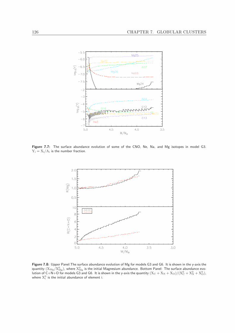
126 CHAPTER 7. GLOBULAR CLUSTERS
Figure 7.7: The surface abundance evolution of some of the CNO, Ne, Na, and Mg isotopes in model G3.Yi = Xi/Ai is the number fraction.
Figure 7.8: Upper Panel:The surface abundance evolution of Mg for models G3 and G6. It is shown in the y-axis thequantity (XMg/X
0Mg), where X0
Mg is the initial Magnesium abundance. Bottom Panel: The surface abundance evo-lution of C+N+O for models G3 and G6. It is shown in the y-axis the quantity (XC +XN +XO)/(X
0C +X0
N +X0O),
where X0i is the initial abundance of element i.

7.3. RESULTS 127
in agreement with previous calculations by Fenner et al. (2004).Ventura & D’Antona (2005a) have explored the role of convection in the discrepancies
between the results by different groups. They have shown that the efficiency of the convectionmodel adopted has a strong influence on the nucleosynthesis that happens at the bottom of theconvective envelope. They found that models adopting the Full Spectrum of Turbulence (FST)treatment of convection developed by Canuto & Mazzitelli (1991) achieve larger luminositiesthan models adopting MLT. Therefore, models adopting FST have a shorter AGB evolution.Moreover, they have found that FST models have steeper radiative temperature gradientprofiles, which favors a more internal position of the inner border of the convective envelopewhich may overlap the CNO burning shell. This has a strong impact in the nucleosynthesis atthe bottom of the convective envelope, leading to a strong depletion of oxygen and magnesium.
Our models using MLT achieve temperatures at the bottom of the convective enve-lope as large as those found by Ventura & D’Antona (2005a) using FST (for instance, seetheir Figure 2). This should lead to similar oxygen depletion in our models. Furthermore,Ventura & D’Antona (2005b) have argued that the difference in convection efficiency betweentheir models and Fenner et al. (2004) is in the core of the increase in C+N+O observed inthe models simulated by the latter. In fact, in their models using MLT, Ventura & D’Antona(2005a) have found an increase in C+N+O of 0.4-0.8 dex, depending on the value chosenfor the mixing length parameter, contrary to their FST model that shows no increase in theC+N+O abundance.
Our models present similar Tbce as those found in models by Ventura & D’Antona (2005a)using FST, but have much stronger TDU efficiencies than their models (this can be seen inthe sudden increase in 12C abundance observed at each TP in our models - Figure 7.7). Inorder to test whether our models using MLT would also present CNO enhancement if theTDU efficiency is reduced, we have performed additional models without overshooting.
Model G7 uses the same physical inputs as our standard models (see Table 7.1), ex-cept that in this model no overshooting was included and the mass-loss rate is calculatedaccording to Bloecker (1995) with a free parameter η = 0.02, which is the same used byVentura & D’Antona (2005b). As it can been seen by the large decrease in the 12C abun-dance in Figure 7.9, the absence of overshooting supress the TDU at the beginning of theAGB. 16O and 24Mg are depleted, while the 14N and 25Mg surface abundances increase. TDUsets in later on, slightly increasing 12C abundance. The lack of fresh 12C due to the low effi-ciency of TDU, leads to a smaller increase in 14N abundance when compared to our standardmodels. While the 14N abundance increases by ∼ 2.0 dex in model G3, it increases by only∼ 1.0 dex in model G7.
The upper panel in Figure 7.9 shows that, contrary to our standard models, the sum ofthe CNO abundances does not increase. Moreover, the total magnesium abundance slightlydecreases in the model without overshooting. In their calculations, Ventura & D’Antona(2005b) do not include overshooting in the inner border of the convective envelope. Thus, themain difference between their models and model G7 would be the convection model adoptedand the low temperature opacities used. Model G7 indicates that the inclusion of overshootingin the inner border of the convective envelope, which determines the efficiency of TDU, playsa more important role in the final C+N+O sum and in the total Mg abundance than theconvection model used.
Recent measurements of the C+N+O abundance have confirmed earlier findings that thisquantity is constant in GCs (Carretta et al. 2005; Villanova et al. 2010). Observations byYong et al. (2009) for NGC 1851, however, have shown a variable C+N+O in this cluster. Al-
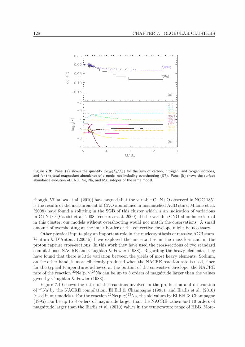
128 CHAPTER 7. GLOBULAR CLUSTERS
Figure 7.9: Panel (a) shows the quantity log10(Xi/X0i ) for the sum of carbon, nitrogen, and oxygen isotopes,
and for the total magnesium abundance of a model not including overshooting (G7). Panel (b) shows the surfaceabundance evolution of CNO, Ne, Na, and Mg isotopes of the same model.
though, Villanova et al. (2010) have argued that the variable C+N+O observed in NGC 1851is the results of the measurement of CNO abundance in mismatched AGB stars, Milone et al.(2008) have found a splitting in the SGB of this cluster which is an indication of variationsin C+N+O (Cassisi et al. 2008; Ventura et al. 2009). If the variable CNO abundance is realin this cluster, our models without overshooting would not match the observations. A smallamount of overshooting at the inner border of the convective envelope might be necessary.
Other physical inputs play an important role in the nucleosynthesis of massive AGB stars.Ventura & D’Antona (2005b) have explored the uncertanties in the mass-loss and in theproton capture cross-sections. In this work they have used the cross-sections of two standardcompilations: NACRE and Caughlan & Fowler (1988). Regarding the heavy elements, theyhave found that there is little variation between the yields of most heavy elements. Sodium,on the other hand, is more efficiently produced when the NACRE reaction rate is used, sincefor the typical temperatures achieved at the bottom of the convective envelope, the NACRErate of the reaction 22Ne(p, γ)23Na can be up to 3 orders of magnitude larger than the valuesgiven by Caughlan & Fowler (1988).
Figure 7.10 shows the rates of the reactions involved in the production and destructionof 23Na by the NACRE compilation, El Eid & Champagne (1995), and Iliadis et al. (2010)(used in our models). For the reaction 22Ne(p, γ)23Na, the old values by El Eid & Champagne(1995) can be up to 8 orders of magnitude larger than the NACRE values and 10 orders ofmagnitude larger than the Iliadis et al. (2010) values in the temperature range of HBB. More-

7.3. RESULTS 129
over, in this temperature range, the rates of the destruction reactions are always smaller thanthe production rates in the NACRE and El Eid & Champagne (1995) cases. On the otherhand, for high temperatures (0.07 ≤ Tbce/T9 ≤ 1.1) the rate for the reaction 22Ne(p, γ)23Nabecomes smaller than the rates for the reactions 23Na(p, γ)24Mg and 23Na(p, α)20Ne in thenewest compilation (Iliadis et al. 2010). This could explain, for instance, the ∼ 1.0 dex differ-ence between Fenner et al. (2004) and our sodium yields for the 5.0M⊙ models, since they usedthe rate values by El Eid & Champagne (1995) and we used the newest rates by Iliadis et al.(2010).
Yong et al. (2003) have reported that 24Mg is the most abundant Mg isotope in theGC NGC 6752. They have found that in the least polluted stars the Mg isotopic ratio is24Mg : 25Mg : 26Mg ∼ 80 : 10 : 10, while in those most polluted it is 24Mg : 25Mg : 26Mg∼ 60 : 10 : 30. Yong et al. (2006) have found similar Mg isotopic ratios for the GCs M13 andM71. Our predictions are in conflict with these observations, since 24Mg is extremely depleteddue to HBB, while 25Mg is produced. Our surface isotopic ratios are 24Mg : 25Mg : 26Mg∼ 1 : 57 : 42 and 24Mg : 25Mg : 26Mg ∼ 1 : 91 : 8 for models G3 and G7, respectively. Theseinconsistencies were also obtained by other author in the literature (e.g. Denissenkov & Herwig(2003)). D’Ercole et al. (2008) have performed hydrodynamical simulations of star formationfor the second generation in GCs. They have explored in their models the possibility thatthe second generation (SG) stars were formed from material containing a mixing of the AGBand super-AGB3 ejectas with the pristine matter. Using this assumption they were able toreproduce the observed helium distribution for the SG stars of NGC 2808. For this rea-son, Ventura et al. (2011) have argued that in the framework of a dilution model the Mgisotopic-ratios problem could be solved. The pristine matter is expected to have the 24Mgabundance enhanced by 0.4 dex, while 25Mg and 26Mg have solar-scaled abundances. Hence,dilution between the AGB ejecta and the pristine material should result in a decrease in 25Mgabundance.
One possible way to discriminate between the two polluters (AGB stars or fast-rotatingmassive stars) is a comparison between the lithium abundance in the first and second gener-ation stars (D’Antona et al. 2012). AGB stars produce lithium at the beginning of the HBB,while massive stars destroy it. This difference should be reflected in the lithium abundancein the SG stars. Recent lithium abundance measurements in stars of NGC 6752 have shownthat there is a correlation between lithium and oxygen (Shen et al. 2010). However, it wasobserved that the Li depletion is smaller than the O depletion. This means that lithiummust be produced in the polluting stars. The high temperatures at the bottom of the convec-tive envelope activate the reaction 3He(α, γ)7Be. 7Be is then converted into 7Li while beingtransported to the surface, where it survives because the temperature is too low for the oc-currence of proton capture. Figure 7.11 shows the 7Li abundance for models G1-G3 and G7.It can be observed an initial phase of lithium production, where lithium abundance reachesthe maximum value of logǫ(Li) = 4.0, that lasts until the exhaustion of 3He in the envelope.Figure 7.11 also shows that the smaller the initial stellar mass, the slower is the decrease ofthe lithium abundance. Moreover, our 3.0M⊙ model never reaches values of logǫ(Li) largerthan ∼ 1.0 dex. Models by Ventura & D’Antona (2008) for the same metallcitiy, on the otherhand, show similar maximum lithium surface abundances for all masses (logǫ(Li) ∼ 4.0). Thisdifference is the result of the larger Tbce values found by Ventura & D’Antona (2008) for their
3Super-AGB stars are stars with masses M ∼ 7− 11M⊙, in the TP-AGB phase, which are the progenitorsof oxygen-neon white dwarfs.
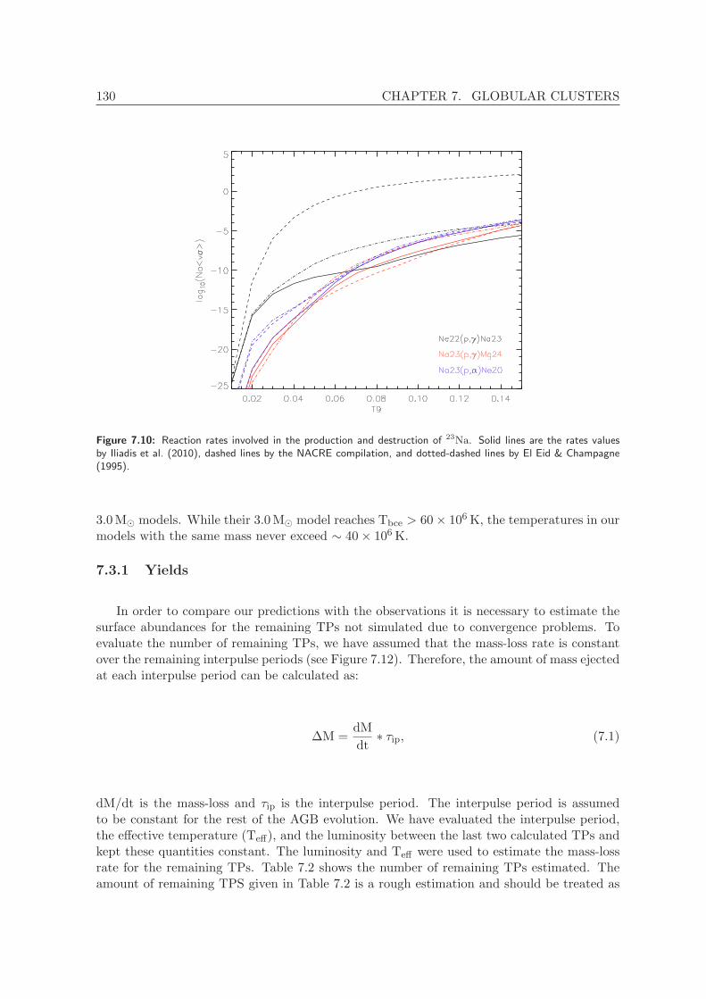
130 CHAPTER 7. GLOBULAR CLUSTERS
Figure 7.10: Reaction rates involved in the production and destruction of 23Na. Solid lines are the rates valuesby Iliadis et al. (2010), dashed lines by the NACRE compilation, and dotted-dashed lines by El Eid & Champagne(1995).
3.0M⊙ models. While their 3.0M⊙ model reaches Tbce > 60× 106K, the temperatures in ourmodels with the same mass never exceed ∼ 40× 106K.
7.3.1 Yields
In order to compare our predictions with the observations it is necessary to estimate thesurface abundances for the remaining TPs not simulated due to convergence problems. Toevaluate the number of remaining TPs, we have assumed that the mass-loss rate is constantover the remaining interpulse periods (see Figure 7.12). Therefore, the amount of mass ejectedat each interpulse period can be calculated as:
∆M =dM
dt∗ τip, (7.1)
dM/dt is the mass-loss and τip is the interpulse period. The interpulse period is assumedto be constant for the rest of the AGB evolution. We have evaluated the interpulse period,the effective temperature (Teff), and the luminosity between the last two calculated TPs andkept these quantities constant. The luminosity and Teff were used to estimate the mass-lossrate for the remaining TPs. Table 7.2 shows the number of remaining TPs estimated. Theamount of remaining TPS given in Table 7.2 is a rough estimation and should be treated as

7.3. RESULTS 131
Figure 7.11: Lithium surface abundance (logǫ(Li) = log(NLi/NH) + 12) evolution for models G1-G3 and G7. Thelithium-rich phase lasts while 3He is not exhausted in the surface. M represents the total mass of the star as afunction of time (M(t)).
an upper limit. For instance, the effective temperature is expected to decrease with each TP,which in turn should increase the mass-loss rate of the following TP.
Model Extra TPs λ
G1 1 0.90G2 4 1.51G3 17 1.21G4 0 0.74G5 10 1.08G6 17 1.18G7 3 0.11G8 0 0.11G9 7 0.11
Table 7.2: Number of remaining TPs.
To estimate the enrichment of the envelope from the remaining TPs, we need four pieces ofinformation from the detailed AGB calculations: 1) the TDU efficiency (λ), 2) the compositionof the intershell, 3) the composition of the envelope in the last calculated model, and 4) themass by which the H-exhausted core grows (∆MH). λ, ∆MH, and the composition of theintershell are assumed constant during the remaining TPs.
The efficiency of the TDU is defined as the ratio of the mass dredged-up by the envelope,∆Md,to the increase in the H-free core mass due to H-burning during the interpulse period, ∆MH
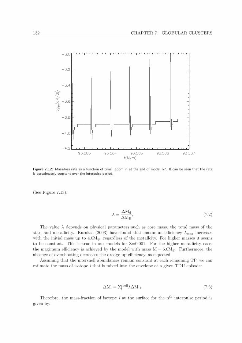
132 CHAPTER 7. GLOBULAR CLUSTERS
Figure 7.12: Mass-loss rate as a function of time. Zoom in at the end of model G7. It can be seen that the rateis aproximately constant over the interpulse period.
(See Figure 7.13),
λ =∆Md
∆MH, (7.2)
The value λ depends on physical parameters such as core mass, the total mass of thestar, and metallicity. Karakas (2003) have found that maximum efficiency λmax increaseswith the initial mass up to 4.0M⊙, regardless of the metallcity. For higher masses it seemsto be constant. This is true in our models for Z=0.001. For the higher metallicity case,the maximum efficiency is achieved by the model with mass M = 5.0M⊙. Furthermore, theabsence of overshooting decreases the dredge-up efficiency, as expected.
Assuming that the intershell abundances remain constant at each remaining TP, we canestimate the mass of isotope i that is mixed into the envelope at a given TDU episode:
∆Mi = Xshelli λ∆MH. (7.3)
Therefore, the mass-fraction of isotope i at the surface for the nth interpulse period isgiven by:

7.3. RESULTS 133
Figure 7.13: Schematic definition of the dredge-up efficiency.
Xni =
(Mnenv − λδMH)X
n−1i +∆Mi
Mnenv
, (7.4)
Xn−1i is the mass-fraction of isotope i at the surface for the (n− 1)th interpulse period and
Mnenv is the current envelope mass.
The surface abundance estimated is an upper limit for many isotopes, since we are assum-ing that only TDU is happening, and that HBB is neglegible, which is not true in the highmass models (M ≥ 4.0M⊙).
Figure 7.14 shows the variation in the lithium integrated abundance in the ejecta as a func-tion of initial mass for our models and for models by (Ventura et al. 2009; Ventura & D’Antona2010) of metallicity Z=0.001. Except for M = 4.0M⊙, our models underproduce lithium incomparison to Ventura et al. (2009) models. However, the largest differences are found whencomparing the standard models. As explained in Section 7.3, models with 3.0M⊙ achievetemperatures at the bottom of the convective envelope much smaller than those found byVentura et al. (2009). For instance, the maximum temperature achieved in our model G8is Tmax
bce = 35× 106K, while Ventura et al. (2009) found Tmaxbce = 73× 106K for their 3.0M⊙
model. The difference in the rate of the reaction 3He(α, γ)7Be between these two temperaturesis of about three orders of magnitude, which should explain the smaller lithium productionin our 3.0M⊙ models.
For the 5.0M⊙ model, the longer lithium production phase in the model without over-shooting is responsible for the discrepancies between model G3 and G7 (see Figure 7.11). Theaverage lithium content of the ejecta is determined by the mass lost during the productionphase (Ventura & D’Antona 2008). The larger the mass lost during the lithium-rich phase is,the larger is the final yield.
The final sodium abundance of the ejecta is determined by the efficiency of TDU indredging-up 22Ne from the ashes of He-burning shell, increasing 23Na abundance, and by
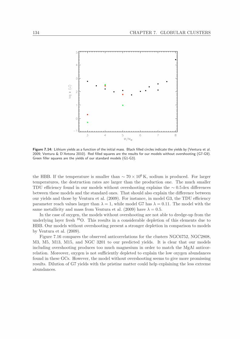
134 CHAPTER 7. GLOBULAR CLUSTERS
Figure 7.14: Lithium yields as a function of the initial mass. Black filled circles indicate the yields by (Ventura et al.2009; Ventura & D’Antona 2010). Red filled squares are the results for our models without overshooting (G7-G9).Green filler squares are the yields of our standard models (G1-G3).
the HBB. If the temperature is smaller than ∼ 70× 106K, sodium is produced. For largertemperatures, the destruction rates are larger than the production one. The much smallerTDU efficiency found in our models without overshooting explains the ∼ 0.5 dex differencesbetween these models and the standard ones. That should also explain the difference betweenour yields and those by Ventura et al. (2009). For instance, in model G3, the TDU efficiencyparameter reach values larger than λ = 1, while model G7 has λ = 0.11. The model with thesame metallicity and mass from Ventura et al. (2009) have λ = 0.5.
In the case of oxygen, the models without overshooting are not able to dredge-up from theunderlying layer fresh 16O. This results in a considerable depletion of this elements due toHBB. Our models without overshooting present a stronger depletion in comparison to modelsby Ventura et al. (2009).
Figure 7.16 compares the observed anticorrelations for the clusters NGC6752, NGC2808,M3, M5, M13, M15, and NGC 3201 to our predicted yields. It is clear that our modelsincluding overshooting produces too much magnesium in order to match the MgAl anticor-relation. Moreover, oxygen is not sufficiently depleted to explain the low oxygen abundancesfound in these GCs. However, the model without overshooting seems to give more promissingresults. Dilution of G7 yields with the pristine matter could help explaining the less extremeabundances.

7.3. RESULTS 135
Figure 7.15: Upper Pannel: Sodium yields as a function of the initial mass. Bottom Pannel: Oxygen yields as afunction of the initial mass. Black filled circles indicate the yields by (Ventura et al. 2009; Ventura & D’Antona2010). Red filled squares are the results for our models without overshooting (G7-G9). Green filler squares are theyields of our standard models (G1-G3). Orange filled triangles indicate the yields by Fenner et al. (2004).
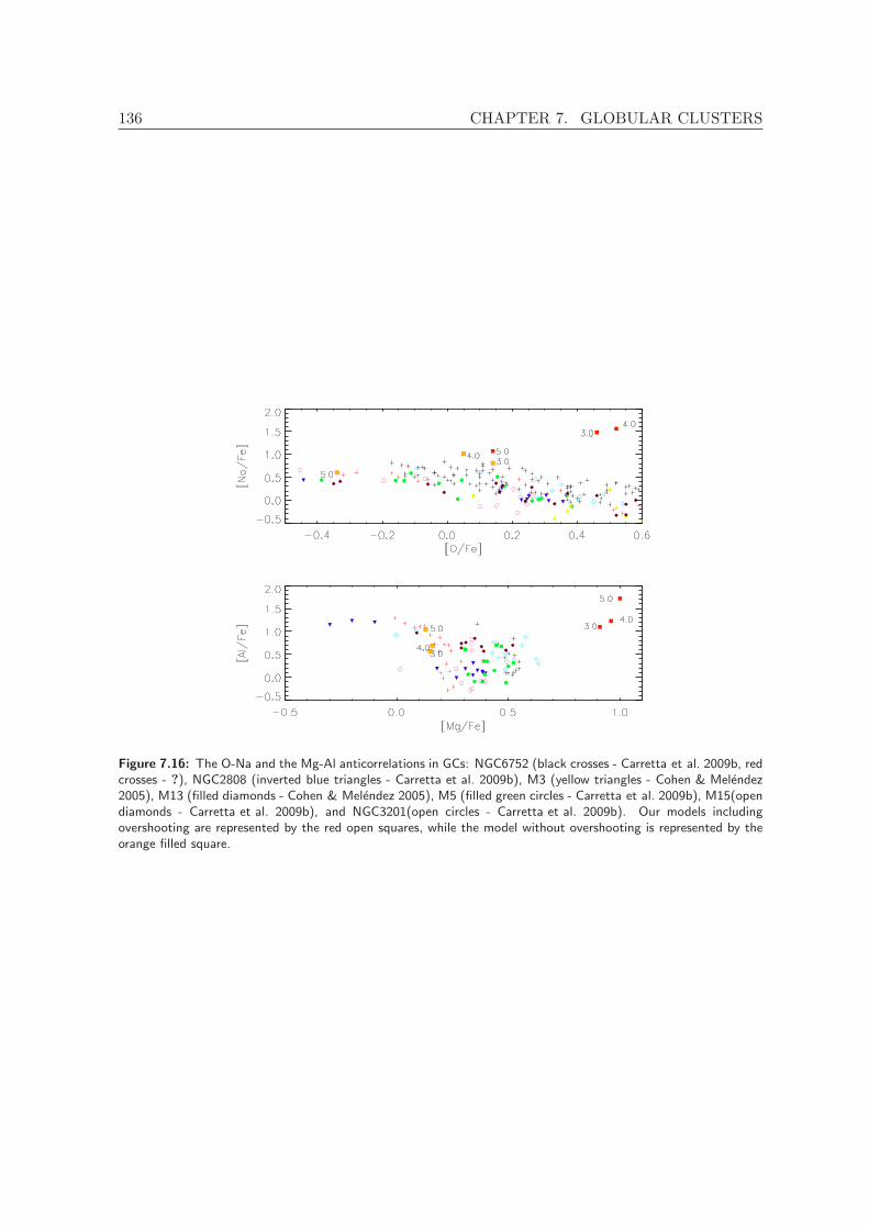
136 CHAPTER 7. GLOBULAR CLUSTERS
Figure 7.16: The O-Na and the Mg-Al anticorrelations in GCs: NGC6752 (black crosses - Carretta et al. 2009b, redcrosses - ?), NGC2808 (inverted blue triangles - Carretta et al. 2009b), M3 (yellow triangles - Cohen & Melendez2005), M13 (filled diamonds - Cohen & Melendez 2005), M5 (filled green circles - Carretta et al. 2009b), M15(opendiamonds - Carretta et al. 2009b), and NGC3201(open circles - Carretta et al. 2009b). Our models includingovershooting are represented by the red open squares, while the model without overshooting is represented by theorange filled square.

7.4. CONCLUSIONS 137
7.4 Conclusions
We present AGB models of intermediate-mass stars with metallicities Z=0.001 and Z=0.004.We have used in these calculations the most up to date reaction rates, specially for thosereactions involved in the NeNa and MgAl chains. Our standard models uses the variable C/Olow-temperature opacities and different mass-loss rates for c-rich and o-rich atmospheres.Overshooting was used in all convective boundaries in these models.
Our standard models present similar problems as earlier publications (Denissenkov & Herwig2003; Fenner et al. 2004): a large increase in the C+N+O values and an increase in the totalmagnesium abundance. Our models produce much stronger sodium enhancement than theobserved in GCs. However, our 5.0M⊙ models do not produce as much sodium as found byFenner et al. (2004). This is probably due to the use of up to date reactions rates for thereaction 22Ne(p, γ)23Na. The old values used by them, can be several orders of magnitudelarger than those used in our calculations. Moreover, the new reaction rate values show thatfor high temperatures the sodium production reaction is smaller than its destruction reaction,which causes a decrease in the sodium abundance towards the end of the AGB evolution.
In attempt to understand the role extra mixing in the inner border of the convectiveenvelope plays in these results, we have performed models without overshooting. This modelis able to reproduce some of the observed features. In figure 7.16, it can be seen that thenon-overshooting model matches the observed O-Na and Mg-Al anticorrelations much morethan our standard models. The Mg istopic-ratio is quite different form the observed value.While in our models 25Mg is most abundant isotope, the observations show that 24 is themost abundant. Recent hydrodinamical simulations of the second generation star formation,however, show that it is possible that the AGB and super-AGB ejectas are mixed with pristinematerial. This should solve the isotopic-ratio problem.
Concerning the question whether AGB stars are responsible for the star-to-star variationsobserved in GCs: they still cannot be ruled out as the possible GC polluters. Althoughovershooting is expected to occur, it is not clear by how far must the convective zone over-shoot. The amount of overshooting should depend on the stellar parameters and it could besufficiently small in the envelope of massive AGB stars in order to match the observations.Moreover, our results shows that the amount if extra mixing plays a more important role inthe differences between our yields and those from Ventura and collaborators work than thedifference in convection theory used.

138 CHAPTER 7. GLOBULAR CLUSTERS

Chapter 8Summary and Conclusions
In the course of this thesis we have explored the evolution and nucleosynthesis of extremelymetal-poor and zero metallicity stars. Stars with a tiny amount of metal in their composi-tion usually suffers the, so called, proton ingestion episode. The conditions in which thisphenomenon happens strongly depends on the treatment of convection and mixing. For starswith initial mass 2.0M⊙ our results are in good agreement with previous studies regarding themetallicity boundaries for such phenomenon. Our models with stellar mass 3.0M⊙ undergoPIE up to Z = 10−5. This is very different from what has been found in the literature. Infact, for this mass, there is a large discrepancy between all the studies.
The ingestion of protons into the C-rich convective zone results in a substantial productionof neutrons, and therefore, s-process elements. This neutron production was found for bothlow- and intermediate-mass stars in our models. Fujimoto et al. (2000) have claimed that low-mass stars, which undego PIE during the He-flash, do not produce s-process due to the shortduration of the PIE. Our models, however, agree with the findings by Campbell et al. (2010)that s-process production does occur in low-mass stars. Nevertheless, the final surface enrich-ment resulting from this phenomenon is significant different from that found Campbell et al.(2010). The neutron superburst found in their models was not reproduced in our calculations.The nature of this superburst is rather puzzling, since the zone where it occurs is extremelyrich in 12C which is an important neutron poison in this condition.
In Chapter 5 we have expanded the work by Campbell et al. (2010) to more metallici-ties and masses. Our models have surface s-process enrichment ≥ 2.0 dex smaller than thatfound in this work. This leads to different conclusions concerning the two most iron-poor stars(HE1327-2623 and HE0107-5240). Whilst their model can reproduce the abundance pattern ofHE1327-2623, the smaller production in our model matches the pattern of HE0107-5240. Wealso addressed the main uncertainty in the PIE modelling: convection. Using different over-shooting parameters, we have found that the neutron exposure averaged across the convectivezone is one of the key quantities determining the final s-process abundance. Moreover, theneutron density time evolution is the major difference between our model and Campbell et al.(2010). For the light elements, we have shown that some have their final abundance deter-mined by the PIE conditions, while others (Li,N) depend strongly on the time between thesplitting of the convective zone and the start of the post-PIE dredge-up.
In Chapter 6 we have performed for the first time s-process calculations for the PIE phasein EMP and zero metallicity intermediate-mass stars. We have found once again that s-

140 CHAPTER 8. SUMMARY AND CONCLUSIONS
processing during the PIE depends on the duration of the proton ingestion (∆tPIE). Ourmodels present a large range of ∆tPIE: varying from ∼ 10−4 yrs to ∼ 7 × 10⁻¹ yrs. Theresults do not seem to have a trend with mass, however, for the 2.0M⊙ models, we foundthat this quantity increases with metallicity. This leads to significant larger enhancements ins-process elements after the PIE in the high metallicity models (for instance, models I3 and I8have [Ba/Fe]=0.01 and 2.15, respectively). We also explore the s-process production after thePIE. Our models have small 13C pocket efficiencies leading in unexpressive neutron densitiesduring the interpulse period. This low efficiency can be ascribed to the low metallicity ofour models, since in this conditions 22Ne becomes an important neutron poison (22(n, γ)23Ne)as was demonstrated by Bisterzo et al. (2010) for models with initial metallicity significantlyhigher than ours. Furthermore, our models show that the interpulse period following theTP in which PIE occurs has the most efficient 13C pocket. For this reason, the bulk of thes-process is formed in these two TPs. However, further investigation into the role played bythe chosen overshooting parameter in the pocket efficiency in this low metallicity regime isnecessary.
We have compared the 2.0M⊙ models with abundances from HE1327-2623 and HE0107-5240. We found that the model with Z = 10−7 is in better agreement with the abundancepatterns observed in HE0107-5240. This agrees with the mass range for the companion starsuggested by Nishimura et al. (2009) based on their parametric study of the PIE. Nonetheless,the large uncertainties in the PIE modelling do not allow low-mass stars to be dismissed asthe HE0107-5240. For HE1327-2623, the 2.0M⊙ model has a better agreement than the LMcase. However, we did not find the large enhancement in Sr observed in this star.
For the light elements, large discrepancies between our results and those reported byCampbell (2007) were found. The differences for most of the light elements can be ascribedto the occurrence of HBB in their models found in none of the models in our grid. Our codeuses the new varying C/O opacities which play an important role in the evolution. They areimportant in such low metallicity environment due to the enrichment in CNO elements in thepost-PIE dredge-up, enhancing the metallicity to Z ∼ 10−4 already in first TP(s). Also, weuse a mass-loss prescription for C-rich stars which result in a large difference in the numberof TPs compared to Campbell (2007) results.
Finally, we made use of the new extended proton-capture network in GARSTEC to addressthe globular cluster anomalies issue. Stars in globular clusters (GC) were believed to be partof one single population. However, detailed spectroscopic analysis have shown that largestar-to-star variations are found among the stars in the cluster, suggesting that cluster arecomposed by more than one stellar population. High accuracy photometry backed up this ideawhen multiple main sequences and red giant branchs were found. The abundance variationsfound in GCs are usually anticorrelated: Na-O and Mg-Al anticorrelations.
One of the possible scenarios to explain these abundance patterns assumes that intermediate-mass stars from the first generation of star polluted the intracluster medium with the materialthat has been subjected to advanced H-burning. Evolutionary calculations for the stars in thefirst generation were mainly performed over the years by Ventura and collaborators. othergroups have reported that their models could not reproduce the observed abundance patterns(Denissenkov & Tout 2003; Fenner et al. 2004). Moreover, they have found that magnesiumwas produced instead of destroyed as expected. Ventura & D’Antona (2005a) have claimedthat sucess of their models in reproducing the observed anticorrelations can be ascribed tothe use of more efficient convection theory. We have performed AGB calculations for starswith 3.0 ≤ M/M⊙ ≤ 5.0 and metallicities Z = 0.001 and Z = 0.004. We found that when over-
141
shooting is included in the calculations our models overproduces Mg. Furthermore, the sumC+N+O that is found to be constant in many GCs is considerably altered during the evo-lution. Additional models without overshooting, however, have shown that it plays a majorrole in the final yields. The absence of overshooting supresses the TDU at the beggining ofthe AGB and, thus, 12C can be transformed into 14N, 16O is also depleted, while 25Mg isconverted into 27Al. Our yields can reproduce the overall Na-O and Mg-Al anticorrelationsobserved.

142 CHAPTER 8. SUMMARY AND CONCLUSIONS

Bibliography
Abel, T., Bryan, G. L., & Norman, M. L. 2002, Science, 295, 93
Adelberger, E. G., Garıa, A., Robertson, R., et al. 2011, RvMP, 83, 195
Alexander, D. R. & Ferguson, J. W. 1994, ApJ, 437, 879
Althaus, L. G., Serenelli, A. M., Panei, J. A., et al. 2005, A&A, 435, 631
Angulo, C., Arnould, M., Rayet, M., Descouvemont, P., & et al. 1999, Nucl. Phys. A, 653, 3
Aoki, W., Beers, T. C., Sivarani, T., et al. 2008, ApJ, 678, 1351
Aoki, W., Norris, J. E., Ryan, S. G., Beers, T. c., & Ando, H. 2002, ApJ, 567, 1166
Beers, T. C. & Christlieb, N. 2005, ARA&A, 43, 531
Beers, T. C., Preston, G., & Shectman, S. 1985, AJ, 90, 2089
Beers, T. C., Preston, G., & Shectman, S. 1992, AJ, 103, 1977
Beers, T. C., Rossi, S., Norris, J. E., Ryan, S. G., & Shefler, T. 1999, AJ, 117, 981
Bessell, M. S., Christlieb, N., & Gustafsson, B. 2004, ApJL, 612, L61
Bidelman, W. & MacConnell, D. 1973, AJ, 78, 687
Bisterzo, S., Gallino, R., Straniero, O., Cristallo, S., & Kappeler, F. 2010, MNRAS, 404, 1529
Bisterzo, S., Gallino, R., Straniero, O., Cristallo, S., & Kappeler, F. 2011, MNRAS, 418, 284
Bloecker, T. 1995, A&A, 297, 727
Bond, H. 1970, ApJS, 22, 117
Bond, H. 1980, ApJS, 44, 517
Bond, H. 1981, ApJ, 248, 606
Boothroyd, A. I., Sackmann, I. J., & Ahern, S. C. 1993, ApJ, 416, 762
Bowen, G. H. 1988, ApJ, 329, 299

144 BIBLIOGRAPHY
Bromm, V., Coppi, P. S., & Larson, R. B. 2002, ApJ, 564, 23
Bromm, V. & Loeb, A. 2003, Nature, 425, 812
Bromm, V. & Loeb, A. 2004, New Astronomy, 9, 353
Busso, M., Gallino, R., & Wasserburg, G. J. 1999, ARAA, 37, 239
Caffau, E., Bonifacio, P., Francois, P., et al. 2011, Nature, 477, 67
Caffau, E., Bonifacio, P., Francois, P., et al. 2012, ArXiv e-prints
Campbell, S. W. 2007, Sructural and Nucleosynthetic Evolution of Metal-Poor and Metal-FreeLow and Intermediate Mass Stars (Monash University, Australia)
Campbell, S. W. & Lattanzio, J. C. 2008, A&A, 490, 769
Campbell, S. W., Lugaro, M., & Karakas, A. I. 2010, A&A, 522, L6
Canuto, V. M. & Mazzitelli, I. 1991, ApJ, 370, 295
Carretta, E., Bragaglia, A., & Cacciari, C. 2004, ApJL, 610, L25
Carretta, E., Bragaglia, A., Gratton, R., D’Orazi, V., & Lucatello, S. 2009a, A&A, 508, 695
Carretta, E., Bragaglia, A., Gratton, R., & Lucatello, S. 2009b, A&A, 505, 139
Carretta, E., Bragaglia, A., Gratton, R. G., et al. 2009c, A&A, 505, 117
Carretta, E., Bragaglia, A., Gratton, R. G., Lucatello, S., & Momany, Y. 2007, A&A, 464,927
Carretta, E., Gratton, R. G., Lucatello, S., Bragaglia, A., & Bonifacio, P. 2005, A&A, 433,597
Cassisi, S., Castellani, V., & Tornambe, A. 1996, ApJ, 459, 298
Cassisi, S., Salaris, M., & Irwin, A. W. 2003, ApJ, 588, 862
Cassisi, S., Salaris, M., Pietrinferni, A., et al. 2008, ApJL, 672, L115
Caughlan, G. R. & Fowler, W. A. 1988, Atomic Data and Nuclear Data Tables, 40, 283
Chieffi, A., Domınguez, I., Limongi, M., & Straniero, O. 2001, ApJ, 554, 1159
Christlieb, N. 2003, RvMA, 16, 191
Christlieb, N., Green, P. J., Wisotzki, L., & Reimers, D. 2001, A&A, 375, 366
Christlieb, N., Gustafsson, B., Korn, A. J., et al. 2004, ApJ, 603, 708
Clayton, D. D. 1983, Principles of stellar evolution and nucleosynthesis, ed. Clayton, D. D.
Cohen, J. G. & Melendez, J. 2005, AJ, 129, 303
Cristallo, S., Gallino, R., & Straniero, O. 2004, Mem. Soc. Astron. Italiana, 75, 174
BIBLIOGRAPHY 145
Cristallo, S., Piersanti, L., Straniero, O., et al. 2009a, PASA, 26, 139
Cristallo, S., Straniero, O., Gallino, R., et al. 2009b, ApJ, 696, 797
Cristallo, S., Straniero, O., & lederer, M. T. 2007, ApJ, 667, 489
Cyburt, R., Amthot, A. M., Ferguson, R., et al. 2010, ApJS, 189, 240
Cyburt, R. H. & Davids, B. 2008, Phys. Rev. C, 78, 064614
D’Antona, F. & Caloi, V. 2004, ApJ, 611, 871
D’Antona, F., Caloi, V., Montalban, J., Ventura, P., & Gratton, R. 2002, A&A, 395, 69
D’Antona, F., D’Ercole, A., Carini, R., Vesperini, E., & Ventura, P. 2012, ArXiv e-prints
Dantona, F. & Mazzitelli, I. 1982, A&A, 113, 303
Decressin, T., Meynet, G., Charbonnel, C., Prantzos, N., & Ekstrom, S. 2007, A&A, 464,1029
Denissenkov, P. A. & Herwig, F. 2003, ApJL, 590, 99
Denissenkov, P. A. & Tout, C. A. 2003, MNRAS, 340, 722
Denissenkov, P. A. & Weiss, A. 1996, A&A, 308, 773
Denissenkov, P. A. & Weiss, A. 2001, ApJL, 559, L115
D’Ercole, A., Vesperini, E., D’Antona, F., McMillan, S. L. W., & Recchi, S. 2008, MNRAS,391, 825
Dillmann, I., Heil, M., Plag, R., Rauscher, T., & Thielemann, F. K. 2006, AIP Conf. Ser.,819, 123
El Eid, M. F. & Champagne, A. E. 1995, ApJ, 451, 298
Fenner, Y., Campbell, S., Karakas, A. I., Lattanzio, J. C., & Gibson, B. K. 2004, MNRAS,353, 789
Ferguson, J. W., Alexander, D. R., Allard, F., et al. 2005, ApJ, 623, 585
Forestini, M. & Charbonnel, C. 1997, A&AS, 123, 241
Frebel, A., Collet, R., Eriksson, K., Christlieb, N., & Aoki, W. 2008, ApJ, 684, 588
Freytag, B., Ludwig, H. G., & Steffen, M. 1996, A&A, 313, 497
Fujimoto, M. Y., Iben, I. J., & Hollowell, D. 1990, ApJ, 349, 580
Fujimoto, M. Y., Ikeda, Y., & Iben, Jr., I. 2000, ApJL, 529, L25
Fynbo, H. O. U., Diget, C. A., Bergmann, U. C., et al. 2005, Nature, 433, 136
Gallino, R., Arlandini, C., Busso, M., et al. 1998, ApJ, 497, 388

146 BIBLIOGRAPHY
Gallino, R., Busso, M., Picchio, G., Raiteri, C. M., & Renzini, A. 1988, ApJ, 334, L45
Goriely, S. & Siess, L. 2001, A&A, 378, 25
Gorres, J., Graff, S., Wiescher, M., et al. 1992, Nuclear Physics A, 548, 414
Gratton, R. G., Bonifacio, P., Bragaglia, A., et al. 2001, A&A, 369, 87
Gratton, R. G., Sneden, C., Carretta, E., & Bragaglia, A. 2000, A&A, 354, 169
Greif, T. H., Springel, V., White, S. D. M., et al. 2011, ApJ, 737, 75
Grevesse, N. & Sauval, A. J. 1998, SSRv, 85, 161
Grundahl, F., Briley, M., Nissen, P. E., & Feltzing, S. 2002, A&A, 385, L14
Hale, S. E., Champagne, A. E., Iliadis, C., et al. 2002, Phys. Rev. C, 65, 015801
Hale, S. E., Champagne, A. E., Iliadis, C., et al. 2004, Phys. Rev. C, 70, 045802
Heger, A. & Woosley, S. E. 2010, ApJ, 724, 341
Herwig, F. 2000, A&A, 360, 952
Herwig, F. 2001, ApJL, 554, L71
Herwig, F. 2005, ARAA, 43, 435
Herwig, F., Blocker, T., Schonberner, D., & El Eid, M. 1997, A&A, 324, L81
Herwig, F., Pignatari, M., Woodward, P. R., et al. 2011, ApJ, 727, 89
Hollowell, D., Iben, I. J., & Fujimoto, M. Y. 1990, ApJ, 351, 245
Iben, Jr., I. & Truran, J. W. 1978, ApJ, 220, 980
Iglesias, C. A. & Rogers, F. J. 1996, ApJ, 464, 943
Iliadis, C., Longland, R., Champagne, A. E., Coc, A., & Fitzgerald, R. 2010, Nuclear PhysicsA, 841, 31
Itoh, N., Mitake, S., Iyetomi, H., & Ichimaru, S. 1983, ApJ, 273, 774
Ivans, I. I., Sneden, C., Kraft, R. P., et al. 1999, AJ, 118, 1273
Iwamoto, N., Kajino, T., Mathews, G. J., Fujimoto, M. Y., & Aoki, W. 2004, ApJ, 602, 377
Iwamoto, N., Umeda, H., Tominaga, N., Nomoto, K., & Maeda, K. 2005, Science, 309, 451
Jaeger, M., Kunz, R., Mayer, A., & et al. 2001, Phys. Rev. Lett., 87, 202501
Jorissen, A. & Arnould, M. 1989, a, 221, 161
Kappeler, F., Beer, H., & Wisshak, K. 1989, Rep. Prog. Phys., 52, 945
Karakas, A. I. 2003, Asymptotic Giant Branch Stars: their influence on binary systems andthe interstellar medium (Monash University, Australia)
BIBLIOGRAPHY 147
Karakas, A. I. 2010, MNRAS, 403, 1413
Karakas, A. I. & Lattanzio, J. . C. 2007, PASA, 20, 279
Karakas, A. I. & Lattanzio, J. C. 2003, PASA, 24, 103
Kippenhahn, R. & Weigert, A. 1990, Stellar Structure and Evolution, ed. Kippenhahn, R. &Weigert, A.
Kitsikis, A. 2008, Theoretical AGB and post-AGB Models for Synthetic Population Studies(Ludwig Maximilians Universitaet, Munich)
Kraft, R. P. 1994, PASP, 106, 553
Kubono, S., Abe, K., Kato, S., & et al. 2003, Phys. rev. Lett., 90, 062501
Kunz, R., Fey, M., Jaeger, M., et al. 2002, ApJ, 567, 643
Langer, N., Heger, A., Wellstein, S., & Herwig, F. 1999, A&A, 346, L37
Lau, H. H. B., Stancliffe, R. J., & Tout, C. A. 2009, MNRAS, 396, 1046
Lederer, M. T. & Aringer, B. 2008, in Evolution and Nucleosynthesis in AGB stars, ed. R.Guandalini, S. Palmerini, & M. Busso, AIP Conf.Ser., 1001, 11
Li, Z., Su, J., Guo, B., et al. 2010, Science in China G: Physics and Astronomy, 53, 658
Lucatello, S., Tsangarides, S., Beers, T. C., et al. 2005, ApJ, 625, 825
Luck, R. E. & Bond. 1991, ApJS, 77, 515
Lugaro, M. 2001, Nucleosynthesis in AGB stars (Monash University, Australia)
Lugaro, M., Herwig, F., Lattanzio, J. C., Gallino, R., & Straniero, O. 2003, ApJ, 586, 1305
Lugaro, M., Karakas, A. I., Stancliffe, R. J., & Rijs, C. 2012, ApJ, 747, 2+
Magic, Z., Serenelli, A., Weiss, A., & Chaboyer, B. 2010, ApJ, 718, 1378
Marigo, P. 2002, A&A, 387, 507
Marigo, P., Girardi, L., Chiosi, C., & Wood, P. R. 2001, A&A, 351, 152
Masseron, T., Johnson, J. A., Plez, B., et al. 2010, A&A, 509, 93
Mattsson, L., Wahlin, R., & Hofner, S. 2010, A&A, 509, 14
Mattsson, L., Wahlin, R., Hofner, S., & Eriksson, K. 2008, A&A, 484, 5
Meyer, B. S. 1994, ARAA, 32, 153
Milone, A. P., Bedin, L. R., Piotto, G., et al. 2008, ApJ, 673, 241
Moazen, B. H., Bardayan, J. C., Blackmon, K. Y., Chae, K. Y., & et al. 2007, Phys. Rev. C,75, 065801

148 BIBLIOGRAPHY
Munakata, H., Kohyama, Y., & Itoh, N. 1985, ApJ, 296, 197
Nishimura, T., Aikawa, M., Suda, T., & Fujimoto, M. Y. 2009, PASJ, 61, 909
O’shea, B. W. & Norman, M. L. 2007, ApJ, 654, 66
Picardi, I., Chieffi, A., Limongi, M., et al. 2004, ApJ, 609, 1035
Piotto, G. 2009, in IAU Symposium, Vol. 258, IAU Symposium, ed. E. E. Mamajek, D. R.Soderblom, & R. F. G. Wyse, 233–244
Piotto, G., Bedin, L. R., Anderson, J., et al. 2007, ApJL, 661, L53
Ramırez, S. V. & Cohen, J. G. 2002, AJ, 123, 3277
Reimers, D. 1975, Circumstellar envelopes and mass loss of red giant stars (Problems in stellaratmospheres and envelopes.), 229–256
Rogers, F. J., Swenson, F. J., & Iglesias, C. A. 1996, ApJ, 456, 902
Rossi, S., Beers, T. C., & Sneden, C. 1999, ASPC, 165, 264
Sbordone, L., Salaris, M., Weiss, A., & Cassisi, S. 2011, A&A, 534, A9
Schaller, G., Schaerer, D., Meynet, G., & Maeder, A. 1992, A&A, 96, 269
Schlattl, H., Cassisi, S., Salaris, M., & Weiss, A. 2001, ApJ, 559, 1082
Schlattl, H., Salaris, M., Cassisi, S., & Weiss, A. 2002, A&A, 395, 77
Schneider, R., Ferrara, A., Salvaterra, R., Omukai, K., & Bromm, V. 2003, Nature, 422, 869
Schoier, F. L. & Olofsson, H. 2001, A&AS, 368, 969
Seeger, P. A., Fowler, W. A., & Clayton, D. D. 1965, ApJS, 11, 121
Serenelli, A. 2006, Nucleosynthesis in Low Mass Very Metal Poor AGB Stars, ed. S. Randich& L. Pasquini, 322
Shen, Z.-X., Bonifacio, P., Pasquini, L., & Zaggia, S. 2010, A&A, 524, L2
Siess, L., Livio, M., & Lattanzio, J. 2002, ApJ, 570, 329
Spite, F. & Spite, M. 1982, A&A, 115, 357
Stacy, A., Greif, T. H., & Bromm, V. 2010, MNRAS, 403, 45
Stacy, A., Greif, T. H., & Bromm, V. 2012, MNRAS, 422, 290
Stancliffe, R. J., Dearborn, D. S. P., Lattanzio, J. C., Heap, S. A., & Campbell, S. W. 2011,ApJ, 742, 121
Straniero, O., Chieffi, A., Limongi, M., et al. 1997, ApJ, 478, 332
Straniero, O., Gallino, R., Busso, M., et al. 1995, ApJ Lett., 440, 85
BIBLIOGRAPHY 149
Suda, T., Aikawa, M., Machida, M. N., Fujimoto, M. Y., & Iben, J. I. 2004, ApJ, 611, 476
Suda, T. & Fujimoto, M. Y. 2010, MNRAS, 405, 177
Suda, T., Fujimoto, M. Y., & Itoh, N. 2007, ApJ, 667, 1206
Suda, T., Katsuta, Y., Yamada, S., et al. 2008, PASJ, 60, 1159
Suda, T., Yamada, S., Katsuta, Y., et al. 2011, MNRAS, 412, 843
Sugimoto, D. & Fujimoto, M. Y. 1978, PASJ, 30, 467
Takahashi, K. & Yokoi, K. 1987, At. Data Nucl. Data Tables, 36, 375
Tomkin, J., Lamnert, D. L., Edvardsson, B., Gustafsson, B., & Nissen, P. E. 1989, A&A, 219,L15
van Loon, J. T., Cioni, M. R. L., Zijlstra, A. A., & Loup, C. 2005, A&A, 438, 273
Vassiliadis, E. & Wood, P. R. 1993, ApJ, 413, 641
Ventura, P., Caloi, V., D’Antona, F., et al. 2009, MNRAS, 399, 934
Ventura, P., Carini, R., & D’Antona, F. 2011, MNRAS, 415, 3865
Ventura, P. & D’Antona, F. 2005a, A&A, 431, 279
Ventura, P. & D’Antona, F. 2005b, A&A, 439, 1075
Ventura, P. & D’Antona, F. 2008, A&A, 479, 805
Ventura, P. & D’Antona, F. 2010, MNRAS, 402, L72
Ventura, P., D’Antona, F., & Mazzitelli, I. 2002, A&A, 393, 215
Ventura, P., D’Antona, F., Mazzitelli, I., & Gratton, R. 2001, ApJL, 550, L65
Villanova, S., Geisler, D., & Piotto, G. 2010, ApJL, 722, L18
Wachter, A., Schroder, K. P., Winters, J. M., Arndt, T. U., & Sedlmayr, E. 2002, A&A, 384,452
Wachter, A., Winters, J. M., Schroder, K. P., & Sedlmayr, E. 2008, A&A, 486, 497
Weiss, A., Cassisi, S., Schlattl, H., & Salaris, M. 2000, A&A, 533, 413
Weiss, A. & Ferguson, J. W. 2009, A&A, 508, 1343
Weiss, A. & Schlattl, H. 2008, Ap&SS, 623, 99
Weiss, A., Schlattl, H., Salaris, M., & Cassisi, S. 2004, A&A, 422, 217
Whitelock, P. A., Feast, M. W., van Loon, J. T., & Zijlstra, A. A. 2003, MNRAS, 342, 86
Willson, L. A. 2000, ARA&A, 38, 573
150 BIBLIOGRAPHY
Winters, J. M., Le Bertre, T., Jeong, K., Nyman, L.-A., & Epchtein, N. 2003, A&A, 409, 715
Yong, D., Aoki, W., & Lambert, D. L. 2006, ApJ, 638, 1018
Yong, D., Grundahl, F., D’Antona, F., et al. 2009, ApJL, 695, L62
Yong, D., Grundahl, F., Lambert, D. L., Nissen, P. E., & Shetrone, M. D. 2003, A&A, 402,985
Yoshida, N., Omukai, K., & Hernquist, L. 2008, Science, 321, 669

Acknowledgments
This work was only possible due to the scientific and moral support from many people.
First. I would like to thank Achim for the opportunity to come to Germany, to MPA andlearn so much. I would like also to thank the MPA directors, the Max-Plack society, and theIMPRS school for the finantial support and the opportunity to grow as a scientist.
I cannot describe how grateful I am to Aldo Serenelli, not only for the scientific support,but also for understanding my difficult moments during the course of this work.
I will be eternally grateful to Silvia Rossi for being so kind and finding a working spacefor me to finish this thesis. Gostaria de agradecer o carinho e suporte quase materno quesenhora me dedicou todos esses anos.
I am pleased to thank the kind and efficient secretaries: Maria Depner, Gabi Kratschmann,and Cornelia Rickl. You were always helpful, kind, and cheerful. Thanks!
I would like to thank my parents (Dorival and Ednalda), and my brothers, Murilo andNıcolas, for the love, support and understanding; Ao meu painho e a minha mainha (Dorivale Ednalda) e aos meus irmaos, Murilo e Nıcolas, pelo amor, carinho e compreensao;
my fiancee, Nelson, for the love and patience to wait for me all these years, even withan ocean between us =D. For believing in me, even when I didn’t do it myself; meu noivo,Nelson, por todo amor a mim dispensado. Por ser meu maior companheiro, em todos osmomentos. Por aguentar meu genio retado e me fazer rir de qualquer bestage;
my friends Ania Raiter - for all the time we spent together dancing, talking nonsense,laughing, eating sweets and the support in the moments of great need, Rodrigo Vieira pelasconversas no skype e e-mails divertidos que sempre trocamos e que me fazem rir. Pelo suportee carinho em 10 anos de amizade., and Nop Wongwathanarat - for all the great momentsinside and outside MPA. For being a great supportive friend. Laura Porter - always providingme with chocolate, good books and series, and with nice words =D, for reading this thesisand helping me to improve it, Martin Henze - for all the good moments on the dance floor(bailando salsa!), for all the nice (or nonsense) movies we have watched together =D, PaulaJofre - for the support in difficult moments, for reading this thesis, and for the friendship.Gostaria de agradecer pelo carinho e companheirismo nesses anos. Stephan Hachinger - forbeing such a nice and good person. Alan Alves Brito - pelas palavras de incentivo e as dancasmaravilhosas =D.
Marcianita, Marcionildo, Pam, and all the good friends that I have met over the yearsthat, even being so far away, found a way to make my life more cheerful. Um muito obrigado

152 BIBLIOGRAPHY
tambem ao Rodolfo que foi, juntamente com a Ania, um anjo me abrigando na casa deles.
“ ... Somos muitos Severinos iguais em tudo na vida: na mesma cabeca grande que a custoe que se equilibra, no mesmo ventre crescido sobre as mesmas pernas finas e iguais tambemporque o sangue, que usamos tem pouca tinta.
... Somos muitos Severinos iguais em tudo e na sina: a de abrandar estas pedras suando-semuito em cima, a de tentar despertar terra sempre mais extinta,
a de querer arrancar alguns rocado da cinza. Mas, para que me conhecam melhor VossasSenhorias e melhor possam seguir a historia de minha vida, passo a ser o Severino que emvossa presenca emigra.”
Joao Cabral de Melo Neto em Morte e Vida Severina