numerical airfoil catalogue including 360° airfoil polars ... · pdf filenumerical airfoil...
TRANSCRIPT
1
Numerical airfoil catalogue including 360° airfoil polars and aeroacoustic footprints Manfred Imiela1, Benjamin Faßmann1, Gerrit Heilers1, Gunther Wilke1 1Institute of Aerodynamics and Flow Technology, DLR, Braunschweig, 38102, Germany
Correspondence to: Manfred Imiela ([email protected]) or Benjamin Faßmann ([email protected]) 5
Abstract. A methodology is presented for generating 360° airfoil polars and aeroacoustic characteristics by means of CFD
and CAA. The aerodynamic procedure is validated against experimental data of the well-known airfoils DU-93-W-210 and
DU-97-W-300. While a better prediction of the aerodynamic coefficients in the range of -30° and 30° is achieved by a
combination of the k-ω SST turbulence model and a C-topology mesh, for the remaining angles of attack more confidence is
gained with the SA negative turbulence model in combination with an O-topology mesh. Therefore the two data sets are 10
subsequently fused to one complete data set using a kriging interpolation approach. The result of ten different airfoils using
the proposed method is presented. For providing the aeroacoustic characteristics for a wide operation range four
computations and a bilinear interpolation are needed, since the aeroacoustic is dependent on the Mach and Reynolds number.
The bilinear interpolation approach is verificated by a comparison between the originally simulated and the emulated result
at a fifth computational set for six different airfoils. The corresponding overall sound pressure level (OASPL) for four angles 15
of attack for these airfoils is presented and the difference between a fully turbulent computation and simulations with fixed
transition is assessed. The aeroacoustic results further include high-fidelity directivity functions.
1 Introduction
The present work is carried out in the scope of the DLR project RoDeO. The goal of the project is the design of a real wind
turbine rotor. While a proper evaluation of the aerodynamics and a sound structural dimensioning is mandatory, the 20
aeroacoustic analysis is an additional goal of the project in order to design a quiet rotor. Therefore the present paper is
focussed on the generation of airfoil polars including aerodynamic coefficients and aeroacoustic characteristics.
During the design process of a wind turbine blade a multitude of load cases has to be considered. Consequently an
engineering model is needed that can handle the amount of computations required. Despite their limitations computer
programs that are based on the Blade Element Method (BEM) method are still widely used for certification and in the first 25
phase of the design process (Snel 2003, Ning 2013) in order to determine the aerodynamic loads. These codes require the
aerodynamic polar tables containing the aerodynamic lift (Cl), drag (Cd) and moment coefficient (Cm) as input. In contrast to
polar tables used for aeronautical applications, aerodynamic coefficients for the use in wind energy applications need to be
provided for the complete range of angles of attack (from 0° to 360°). The generation of such polar tables is by no means
Wind Energ. Sci. Discuss., https://doi.org/10.5194/wes-2017-51Manuscript under review for journal Wind Energ. Sci.Discussion started: 22 November 2017c© Author(s) 2017. CC BY 4.0 License.
2
trivial. Although research has been ongoing for decades the physical phenomena involved – namely accurate stall prediction
and rotational and 3D effects - have not yet completely been understood (Tangler 2005). While quite some progress has been
made in recent years on understanding the phenomenon of rotational augmentation (Gross 2012, Bangga 2016) the methods
adopted in the said publications are still too expensive in order to be applied on a vast number of airfoils. In contrast to the
very expensive methods a manifold number of approximation methods exit for completion of measured or computed data 5
sets in the regular range of angles of attack. These approximation methods are mostly based on a combination of harmonic
functions and require certain empirical input parameters. In most cases measured data is obtained by wind tunnel testing and
subsequently completed and corrected by such methods. The reason for their popularity lies in the easy handling and the
inexpensive evaluation. On the other hand these methods suffer some severe drawbacks, e.g. they “seem incapable of
representing different maximum Cl values in the negative and positive α region” and “they do not seem to capture the 10
peculiarities of the polar in or close to the attached flow region as well as around 180°” (Skrzypiński 2014).
The authors are conscious of the fact that with the application of steady 2D RANS simulations for the complete range of
angles of attack they leave the boundary of validity of this approach. Yet they believe that the results from a steady RANS
simulation will be superior to the results of the commonly applied approximation methods. Since the computation of a
complete polar by means of steady 2D RANS computations can nowadays be achieved within a day, the chosen prospect can 15
be viewed as a good compromise between accuracy and efficiency. The computed polar tables will be based on pure steady
2D computations without corrections. The corrections for dynamic stall and rotational effects are sought to be included by
the comprehensive rotorcraft code that will be used in the RoDeO project.
Wind turbines offer numerous sources of noise. Besides mechanical sources, like the gear box and the generator, there are
aerodynamic (aeroacoustic) sources of sound to be perceived. Aeroacoustic noise dominates the overall sound emission of a 20
wind turbine (Wagner 1996). Numerous sound mechanisms at the rotor blades are differentiated in the literature. These are
separation noise, vortex the shedding noise, tip vortex noise, and turbulent boundary-layer trailing-edge noise (TBL-TEN)
(Brooks 1989). For multi megawatt turbines, the TBL-TEN has been identified to be the prominent sound contribution
(Oerlemans 2007).
For noise prediction, semi empirical tools are widely used, e.g. the NREL NAFNoise (Moriarty 2005). Different sound 25
sources are included in that framework. It is based on the BPM model (Brooks 1989). A model for inflow turbulence noise
by Amiet 1975 is implemented as well. Further, the aerodynamic tool XFOIL (Drela 1987) is also enclosed to NAFNoise.
The same holds for the TNO model (Parchen 1998). All these models can independently be used to predict emitted noise in
the context of wind turbines. In total, they show a good agreement in overall sound pressure levels, but separate validation is
often lacking in detail. 30
The approach within the framework of RoDeO concentrates on the high fidelity numerical investigation of the emitted sound
of the rotor blades, based on 2D computations of TBL-TEN caused by stochastically modelled turbulence. A reduced order
model unites the reliability of highly resolved computations with a fast estimation procedure. Validation will be realized for
each step of the procedure.
Wind Energ. Sci. Discuss., https://doi.org/10.5194/wes-2017-51Manuscript under review for journal Wind Energ. Sci.Discussion started: 22 November 2017c© Author(s) 2017. CC BY 4.0 License.
3
2 Tools & Methodology
2.1 Framework for Generating Aerodynamic Polars
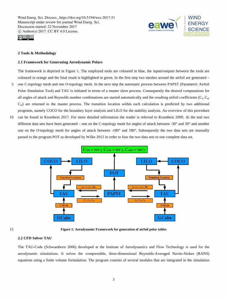
The framework is depicted in Figure 1. The employed tools are coloured in blue, the inputs/outputs between the tools are
coloured in orange and the final result is highlighted in green. In the first step two meshes around the airfoil are generated –
one C-topology mesh and one O-topology mesh. In the next step the automatic process between PAPST (Parametric Airfoil 5
Polar Simulation Tool) and TAU is initiated in terms of a master slave process. Consequently the desired computations for
all angles of attack and Reynolds number combinations are started automatically and the resulting airfoil coefficients (Cl, Cd,
Cm) are returned to the master process. The transition location within each calculation is predicted by two additional
programs, namely COCO for the boundary layer analysis and LILO for the stability analysis. An overview of this procedure
can be found in Krumbein 2017. For more detailed information the reader is referred to Krumbein 2009. At the end two 10
different data sets have been generated – one on the C-topology mesh for angles of attack between -30° and 30° and another
one on the O-topology mesh for angles of attack between -180° and 180°. Subsequently the two data sets are manually
passed to the program POT as developed by Wilke 2012 in order to fuse the two data sets to one complete data set.
Figure 1: Aerodynamic Framework for generation of airfoil polar tables 15
2.2 CFD Solver TAU
The TAU-Code (Schwamborn 2006) developed at the Institute of Aerodynamics and Flow Technology is used for the
aerodynamic simulations. It solves the compressible, three-dimensional Reynolds-Averaged Navier-Stokes (RANS)
equations using a finite volume formulation. The program consists of several modules that are integrated in the simulation
Wind Energ. Sci. Discuss., https://doi.org/10.5194/wes-2017-51Manuscript under review for journal Wind Energ. Sci.Discussion started: 22 November 2017c© Author(s) 2017. CC BY 4.0 License.
4
environment FlowSimulator. This python-based framework performs the coupling between the different modules and allows
in-memory data exchange.
The TAU-Code uses a cell-vertex formulation with a dual-grid approach for the spatial discretization. The solver module
contains a central scheme as well as several upwind schemes for the discretization of the inviscid fluxes. Viscous terms are
computed with a second-order central scheme. For artificial dissipation scalar or matrix dissipation might be chosen by the 5
user. The unstructured code supports the use of hybrid meshes, i.e. mixed type of elements (hexaeder, tetraeder, etc.)
offering more flexibility in the mesh generation process.
Time integration is achieved using either an explicit Runge-Kutta type time-stepping scheme or an implicit LU-SGS (lower-
upper symmetric Gauss-Seidel) algorithm. The time-accurate simulations are performed with an implicit dual-time stepping
approach. Various multi-grid type cycles are available for accelerating the convergence of the flow equations. 10
For the simulation of turbulent flows several one- and two-equation turbulence models are implemented.
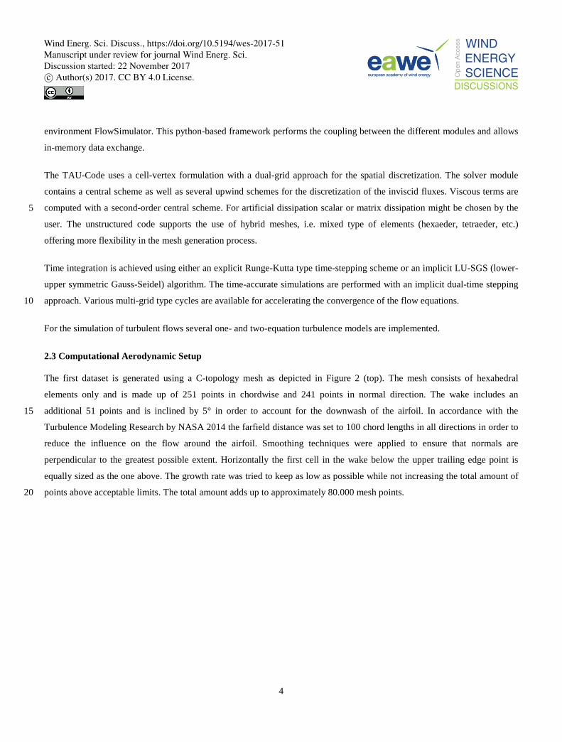
2.3 Computational Aerodynamic Setup
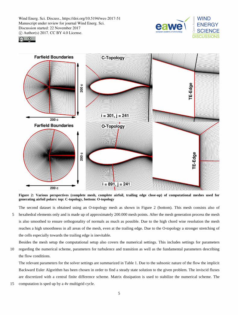
The first dataset is generated using a C-topology mesh as depicted in Figure 2 (top). The mesh consists of hexahedral
elements only and is made up of 251 points in chordwise and 241 points in normal direction. The wake includes an
additional 51 points and is inclined by 5° in order to account for the downwash of the airfoil. In accordance with the 15
Turbulence Modeling Research by NASA 2014 the farfield distance was set to 100 chord lengths in all directions in order to
reduce the influence on the flow around the airfoil. Smoothing techniques were applied to ensure that normals are
perpendicular to the greatest possible extent. Horizontally the first cell in the wake below the upper trailing edge point is
equally sized as the one above. The growth rate was tried to keep as low as possible while not increasing the total amount of
points above acceptable limits. The total amount adds up to approximately 80.000 mesh points. 20
Wind Energ. Sci. Discuss., https://doi.org/10.5194/wes-2017-51Manuscript under review for journal Wind Energ. Sci.Discussion started: 22 November 2017c© Author(s) 2017. CC BY 4.0 License.
5
Figure 2: Various perspectives (complete mesh, complete airfoil, trailing edge close-up) of computational meshes used for generating airfoil polars: top: C-topology, bottom: O-topology
The second dataset is obtained using an O-topology mesh as shown in Figure 2 (bottom). This mesh consists also of
hexahedral elements only and is made up of approximately 200.000 mesh points. After the mesh generation process the mesh 5
is also smoothed to ensure orthogonality of normals as much as possible. Due to the high chord wise resolution the mesh
reaches a high smoothness in all areas of the mesh, even at the trailing edge. Due to the O-topology a stronger stretching of
the cells especially towards the trailing edge is inevitable.
Besides the mesh setup the computational setup also covers the numerical settings. This includes settings for parameters
regarding the numerical scheme, parameters for turbulence and transition as well as the fundamental parameters describing 10
the flow conditions.
The relevant parameters for the solver settings are summarized in Table 1. Due to the subsonic nature of the flow the implicit
Backward Euler Algorithm has been chosen in order to find a steady state solution to the given problem. The inviscid fluxes
are discretized with a central finite difference scheme. Matrix dissipation is used to stabilize the numerical scheme. The
computation is sped up by a 4v multigrid cycle. 15
Wind Energ. Sci. Discuss., https://doi.org/10.5194/wes-2017-51Manuscript under review for journal Wind Energ. Sci.Discussion started: 22 November 2017c© Author(s) 2017. CC BY 4.0 License.
6
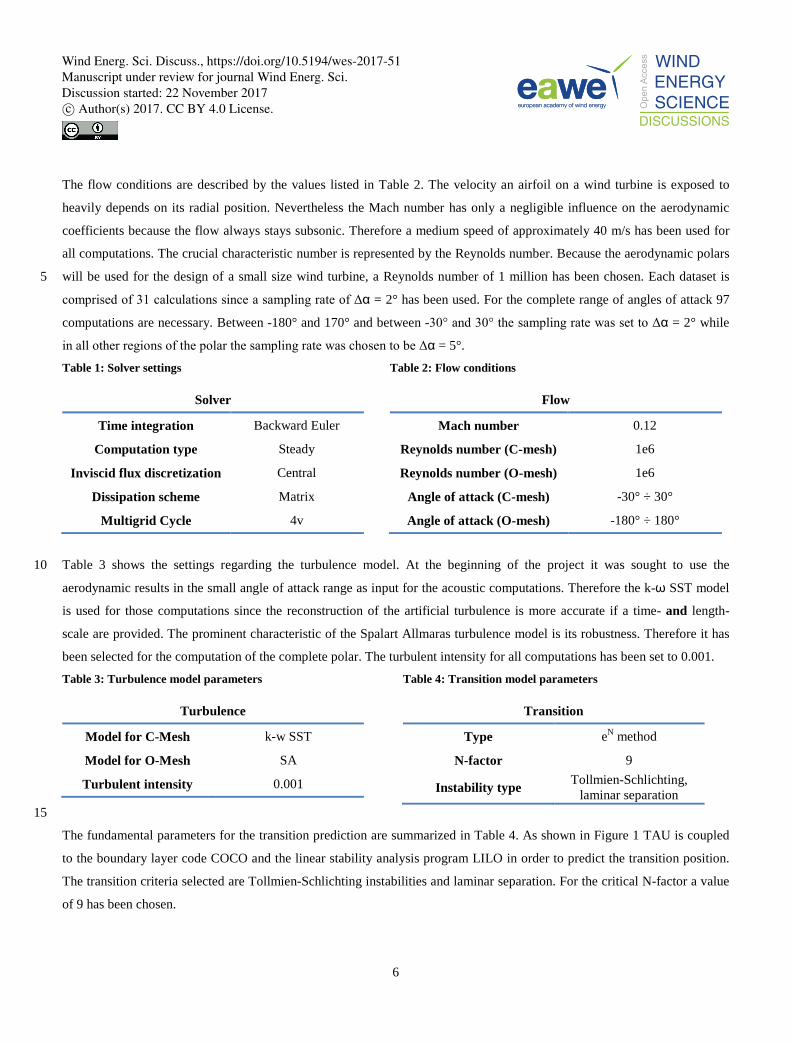
The flow conditions are described by the values listed in Table 2. The velocity an airfoil on a wind turbine is exposed to
heavily depends on its radial position. Nevertheless the Mach number has only a negligible influence on the aerodynamic
coefficients because the flow always stays subsonic. Therefore a medium speed of approximately 40 m/s has been used for
all computations. The crucial characteristic number is represented by the Reynolds number. Because the aerodynamic polars
will be used for the design of a small size wind turbine, a Reynolds number of 1 million has been chosen. Each dataset is 5
comprised of 31 calculations since a sampling rate of Δα = 2° has been used. For the complete range of angles of attack 97
computations are necessary. Between -180° and 170° and between -30° and 30° the sampling rate was set to Δα = 2° while
in all other regions of the polar the sampling rate was chosen to be Δα = 5°.
Table 1: Solver settings
Solver
Time integration Backward Euler
Computation type Steady
Inviscid flux discretization Central
Dissipation scheme Matrix
Multigrid Cycle 4v
Table 2: Flow conditions
Flow
Mach number 0.12
Reynolds number (C-mesh) 1e6
Reynolds number (O-mesh) 1e6
Angle of attack (C-mesh) -30° ÷ 30°
Angle of attack (O-mesh) -180° ÷ 180°
Table 3 shows the settings regarding the turbulence model. At the beginning of the project it was sought to use the 10
aerodynamic results in the small angle of attack range as input for the acoustic computations. Therefore the k-ω SST model
is used for those computations since the reconstruction of the artificial turbulence is more accurate if a time- and length-
scale are provided. The prominent characteristic of the Spalart Allmaras turbulence model is its robustness. Therefore it has
been selected for the computation of the complete polar. The turbulent intensity for all computations has been set to 0.001.
Table 3: Turbulence model parameters
Turbulence
Model for C-Mesh k-w SST
Model for O-Mesh SA
Turbulent intensity 0.001
Table 4: Transition model parameters
Transition
Type eN method
N-factor 9
Instability type Tollmien-Schlichting, laminar separation
15
The fundamental parameters for the transition prediction are summarized in Table 4. As shown in Figure 1 TAU is coupled
to the boundary layer code COCO and the linear stability analysis program LILO in order to predict the transition position.
The transition criteria selected are Tollmien-Schlichting instabilities and laminar separation. For the critical N-factor a value
of 9 has been chosen.
Wind Energ. Sci. Discuss., https://doi.org/10.5194/wes-2017-51Manuscript under review for journal Wind Energ. Sci.Discussion started: 22 November 2017c© Author(s) 2017. CC BY 4.0 License.
7
2.4 Parametric Airfoil Simulation Tool (PAPST)
For generating the airfoil polars a vast number of calculations have to be carried out. For this purpose a set of python based
scripts have been programed by Gerrit Heilers in order to perform all these computations automatically. Although for this
paper only one Reynolds and one Mach number have been chosen, PAPST has been programed to conduct complete DOE
computations with the angle of attack, Reynolds number and Mach number being the design parameters of the DOE. The 5
program contains post-processing routines in order to automatically generate field and pressure plots as for example depicted
in Figure 11 and Figure 17. The computations can be conducted on a local machine as well as done in this case on a cluster
operated by a queueing system. If one or more computations or even the whole DOE crash due to convergence, other
software or hardware errors various techniques for restarting the computations are available. One of PAPST’s main features
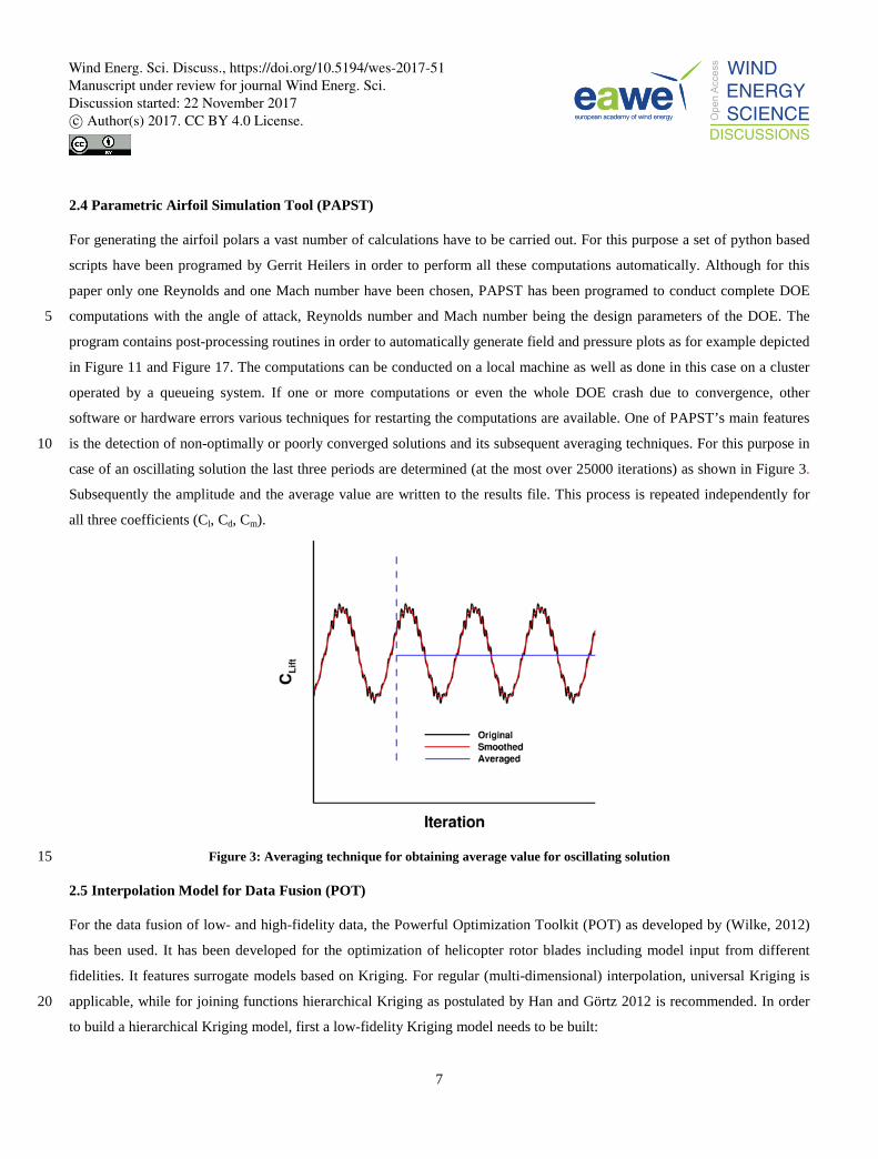
is the detection of non-optimally or poorly converged solutions and its subsequent averaging techniques. For this purpose in 10
case of an oscillating solution the last three periods are determined (at the most over 25000 iterations) as shown in Figure 3.
Subsequently the amplitude and the average value are written to the results file. This process is repeated independently for
all three coefficients (Cl, Cd, Cm).
Figure 3: Averaging technique for obtaining average value for oscillating solution 15
2.5 Interpolation Model for Data Fusion (POT)
For the data fusion of low- and high-fidelity data, the Powerful Optimization Toolkit (POT) as developed by (Wilke, 2012)
has been used. It has been developed for the optimization of helicopter rotor blades including model input from different
fidelities. It features surrogate models based on Kriging. For regular (multi-dimensional) interpolation, universal Kriging is
applicable, while for joining functions hierarchical Kriging as postulated by Han and Görtz 2012 is recommended. In order 20
to build a hierarchical Kriging model, first a low-fidelity Kriging model needs to be built:
Wind Energ. Sci. Discuss., https://doi.org/10.5194/wes-2017-51Manuscript under review for journal Wind Energ. Sci.Discussion started: 22 November 2017c© Author(s) 2017. CC BY 4.0 License.
8
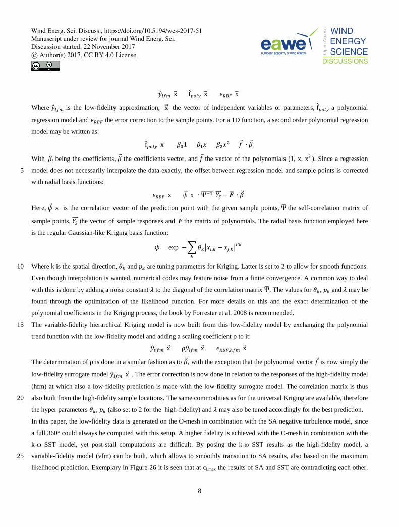
𝑦𝑦�𝑙𝑙𝑙𝑙𝑙𝑙(x�⃗ ) = f̂𝑝𝑝𝑝𝑝𝑙𝑙𝑝𝑝(x�⃗ ) + 𝜖𝜖𝑅𝑅𝑅𝑅𝑅𝑅(x�⃗ )
Where 𝑦𝑦�𝑙𝑙𝑙𝑙𝑙𝑙 is the low-fidelity approximation, (x�⃗ ) the vector of independent variables or parameters, f̂𝑝𝑝𝑝𝑝𝑙𝑙𝑝𝑝 a polynomial
regression model and 𝜖𝜖𝑅𝑅𝑅𝑅𝑅𝑅 the error correction to the sample points. For a 1D function, a second order polynomial regression
model may be written as:
f̂𝑝𝑝𝑝𝑝𝑙𝑙𝑝𝑝(x) = 𝛽𝛽01 + 𝛽𝛽1𝑥𝑥 + 𝛽𝛽2𝑥𝑥2 = 𝑓𝑓 ∙ 𝛽𝛽
With 𝛽𝛽𝑖𝑖 being the coefficients, 𝛽𝛽 the coefficients vector, and 𝑓𝑓 the vector of the polynomials (1, x, x2 ). Since a regression
model does not necessarily interpolate the data exactly, the offset between regression model and sample points is corrected 5
with radial basis functions:
𝜀𝜀𝑅𝑅𝑅𝑅𝑅𝑅(x) = 𝜓𝜓�⃗ (x) ∙ Ψ−1������(𝑌𝑌𝑆𝑆���⃗ − 𝑭𝑭� ∙ 𝛽𝛽)
Here, 𝜓𝜓�⃗ (x) is the correlation vector of the prediction point with the given sample points, Ψ� the self-correlation matrix of
sample points, 𝑌𝑌𝑆𝑆���⃗ the vector of sample responses and 𝑭𝑭� the matrix of polynomials. The radial basis function employed here
is the regular Gaussian-like Kriging basis function:
𝜓𝜓 = exp (−�𝜃𝜃𝑘𝑘�𝑥𝑥𝑖𝑖,𝑘𝑘 − 𝑥𝑥𝑗𝑗,𝑘𝑘�𝑝𝑝𝑘𝑘
𝑘𝑘
)
Where k is the spatial direction, 𝜃𝜃𝑘𝑘 and 𝑝𝑝𝑘𝑘 are tuning parameters for Kriging. Latter is set to 2 to allow for smooth functions. 10
Even though interpolation is wanted, numerical codes may feature noise from a finite convergence. A common way to deal
with this is done by adding a noise constant 𝜆𝜆 to the diagonal of the correlation matrix Ψ� . The values for 𝜃𝜃𝑘𝑘, 𝑝𝑝𝑘𝑘 and 𝜆𝜆 may be
found through the optimization of the likelihood function. For more details on this and the exact determination of the
polynomial coefficients in the Kriging process, the book by Forrester et al. 2008 is recommended.
The variable-fidelity hierarchical Kriging model is now built from this low-fidelity model by exchanging the polynomial 15
trend function with the low-fidelity model and adding a scaling coefficient ρ to it:
𝑦𝑦�𝑣𝑣𝑙𝑙𝑙𝑙(x�⃗ ) = ρ𝑦𝑦�𝑙𝑙𝑙𝑙𝑙𝑙(x�⃗ ) + 𝜖𝜖𝑅𝑅𝑅𝑅𝑅𝑅,ℎ𝑙𝑙𝑙𝑙(x�⃗ )
The determination of ρ is done in a similar fashion as to 𝛽𝛽, with the exception that the polynomial vector 𝑓𝑓 is now simply the
low-fidelity surrogate model 𝑦𝑦�𝑙𝑙𝑙𝑙𝑙𝑙(x�⃗ ). The error correction is now done in relation to the responses of the high-fidelity model
(hfm) at which also a low-fidelity prediction is made with the low-fidelity surrogate model. The correlation matrix is thus
also built from the high-fidelity sample locations. The same commodities as for the universal Kriging are available, therefore 20
the hyper parameters 𝜃𝜃𝑘𝑘, 𝑝𝑝𝑘𝑘 (also set to 2 for the high-fidelity) and 𝜆𝜆 may also be tuned accordingly for the best prediction.
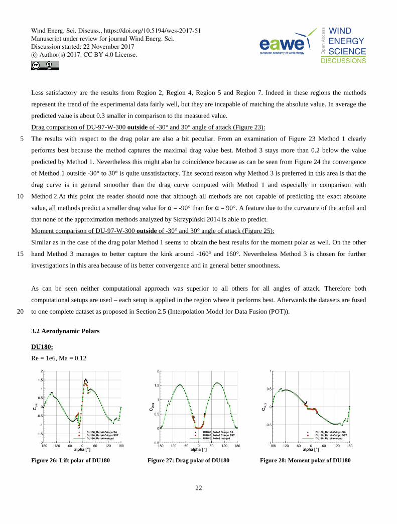
In this paper, the low-fidelity data is generated on the O-mesh in combination with the SA negative turbulence model, since
a full 360° could always be computed with this setup. A higher fidelity is achieved with the C-mesh in combination with the
k-ω SST model, yet post-stall computations are difficult. By posing the k-ω SST results as the high-fidelity model, a
variable-fidelity model (vfm) can be built, which allows to smoothly transition to SA results, also based on the maximum 25
likelihood prediction. Exemplary in Figure 26 it is seen that at cl,max the results of SA and SST are contradicting each other.
Wind Energ. Sci. Discuss., https://doi.org/10.5194/wes-2017-51Manuscript under review for journal Wind Energ. Sci.Discussion started: 22 November 2017c© Author(s) 2017. CC BY 4.0 License.
9
Since high-fidelity data points are still available, the variable-fidelity model still follows this trend. It then gradually drops
onto the SA results around 50° angle-of-attack since no high-fidelity data is available anymore. The data interpolated here
are Cl , Cd and Cm in dependence of the parameter α.
Other ideas for the application may comprise joining CFD and wind tunnel data, which may also be done in a triple-fidelity
setup. Hierarchical Kriging allows to easily chain methods of different fidelities together, since the lower-level model may 5
also be a Hierarchical Kriging model itself.
2.6 Framework for the Aeroacoustic Characterization
The aeroacoustic study in this paper is based on a proven and tested tool chain which was primarily presented by Rautmann
2014. These results were further compared to those of other research teams in the BANC-III-Workshop, Category 1,
Trailing-Edge Noise (Herr 2015). The computational results of the above mentioned procedure show a good agreement to 10
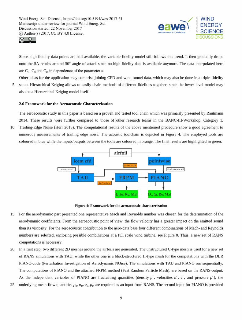
numerous measurements of trailing edge noise. The acoustic toolchain is depicted in Figure 4. The employed tools are
coloured in blue while the inputs/outputs between the tools are coloured in orange. The final results are highlighted in green.
Figure 4: Framework for the aeroacoustic characterization
For the aerodynamic part presented one representative Mach and Reynolds number was chosen for the determination of the 15
aerodynamic coefficients. From the aeroacoustic point of view, the flow velocity has a greater impact on the emitted sound
than its viscosity. For the aeroacoustic contribution to the aero-data base four different combinations of Mach- and Reynolds
numbers are selected, enclosing possible combinations at a full scale wind turbine, see Figure 8. Thus, a new set of RANS
computations is necessary.
In a first step, two different 2D meshes around the airfoils are generated. The unstructured C-type mesh is used for a new set 20
of RANS simulations with TAU, while the other one is a block-structured H-type mesh for the computations with the DLR
PIANO-code (Perturbation Investigation of Aerodynamic NOise). The simulations with TAU and PIANO run sequentially.
The computations of PIANO and the attached FRPM method (Fast Random Particle Mesh), are based on the RANS-output.
As the independent variables of PIANO are fluctuating quantities (density 𝜌𝜌′ , velocities 𝑢𝑢′ , 𝑣𝑣′ , and pressure 𝑝𝑝′ ), the
underlying mean-flow quantities 𝜌𝜌0,𝑢𝑢0, 𝑣𝑣0, 𝑝𝑝0 are required as an input from RANS. The second input for PIANO is provided 25
Wind Energ. Sci. Discuss., https://doi.org/10.5194/wes-2017-51Manuscript under review for journal Wind Energ. Sci.Discussion started: 22 November 2017c© Author(s) 2017. CC BY 4.0 License.
10
by the FRPM tool. Based on the statistics of the kinetic energy of the turbulence 𝑘𝑘, and the specific dissipation rate 𝜔𝜔
provided by the k-ω SST turbulence model from (Menter 1994), the FRPM method reconstructs stochastic turbulence (Ewert
2008). The turbulence statistics from the previous RANS solution is realized, again. The FRPM output provides unsteady
broadband sound sources on a Cartesian background mesh. These generated fluctuations simultaneously excite the PIANO
code, solving e.g. the Acoustic Perturbation Equations (APE), suppressing the vorticity mode in the solution, (Ewert 2003). 5
The propagated acoustic pressure recorded at 360 microphones located on a circle with a radius of 2.5 𝑙𝑙𝑐𝑐 around the trailing
edge. The microphones collect the acoustic farfield signals which include convective amplification as well as refraction and
diffraction effects. This enables the plot of the frequency spectrum 𝐿𝐿𝑝𝑝(𝑓𝑓) for each microphone and the directivity
function 𝐷𝐷Θ. Using this framework, an aeroacoustic data base is assembled.
2.7 Aeroacoustic Solver PIANO and FRPM 10
The PIANO-Code developed at the Institute of Aerodynamics and Flow Technology is used for Computational
AeoroAcoustics (CAA) simulations. As mentioned above, it works in a hybrid two-step procedure. Based on the preceding
RANS computations with the TAU code, in the second step time resolved linear propagations equations like the Linearized
Euler Equations (LEE) or the above mentioned APE are solved on structured multi-block meshes to compute the sound field.
The CAA solver is based on the 4th order accurate DRP scheme proposed by Tam 1993. The temporal discretization is 15
realized by an alternating two-step low-dissipation, low-dispersion Runge-Kutta (LDDRK) algorithm (Hu 1996). The
coefficients are chosen in such a way that the dissipation and dispersion errors are minimized without compromising the
stability limits. Combining two alternating steps in the optimization, the dispersion errors are further reduced and a higher
order of accuracy is maintained.
The left hand side of the linear propagation equations is stimulated by separately applied sound sources at their right hand 20
side. For the computation of trailing edge noise, a vorticity based sound source is imposed, coupled to the CAA solver.
Despite the fact that the APE do not resolve vorticity, they respond on it. The FRPM method realizes these time-resolved
fluctuations from time-averaged turbulence statistics. This Gaussian correlated synthetic turbulence represents the
fluctuating vorticity according to the turbulence statistics of the RANS solution. The source model is the so called ‘Source
A’ under application of the Lamb vector. 25
All acoustic signals can be collected at user-chosen microphones, during simulation. In addition, the temporal and spatial
resolved acoustic quantities can be recorded at user-defined Ffowcks-Williams-Hawkings-Surfaces. These signals are to be
propagated to the farfield separately in a post processing of the data.
2.8 Computational Setup for Aeroacoustics
Based on the procedure presented above, the aeroacoustic investigation was performed according to Figure 4. Meeting as 30
many as possible local flow conditions at different blade elements in the outer 20% of a rotor blade, five different
Wind Energ. Sci. Discuss., https://doi.org/10.5194/wes-2017-51Manuscript under review for journal Wind Energ. Sci.Discussion started: 22 November 2017c© Author(s) 2017. CC BY 4.0 License.
11
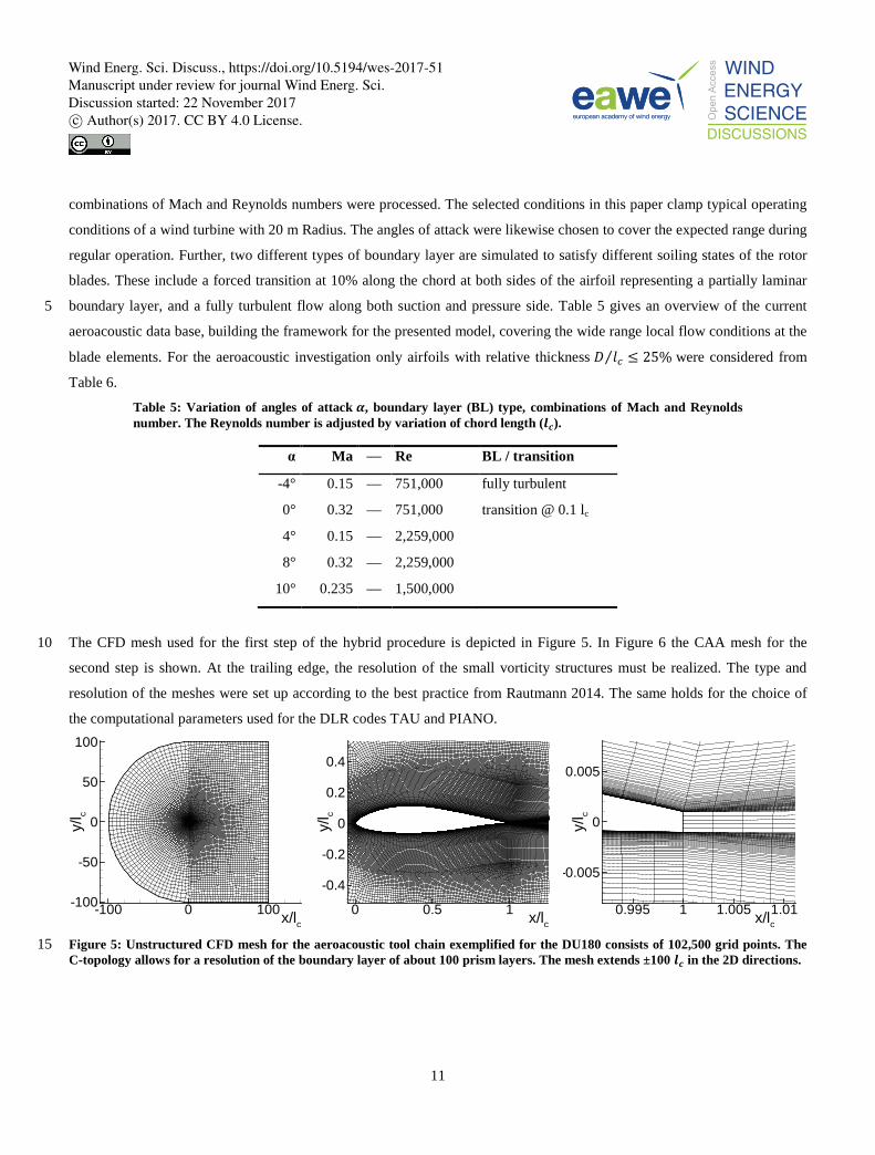
combinations of Mach and Reynolds numbers were processed. The selected conditions in this paper clamp typical operating
conditions of a wind turbine with 20 m Radius. The angles of attack were likewise chosen to cover the expected range during
regular operation. Further, two different types of boundary layer are simulated to satisfy different soiling states of the rotor
blades. These include a forced transition at 10% along the chord at both sides of the airfoil representing a partially laminar
boundary layer, and a fully turbulent flow along both suction and pressure side. Table 5 gives an overview of the current 5
aeroacoustic data base, building the framework for the presented model, covering the wide range local flow conditions at the
blade elements. For the aeroacoustic investigation only airfoils with relative thickness 𝐷𝐷 𝑙𝑙𝑐𝑐⁄ ≤ 25% were considered from
Table 6.
Table 5: Variation of angles of attack 𝜶𝜶, boundary layer (BL) type, combinations of Mach and Reynolds number. The Reynolds number is adjusted by variation of chord length (𝒍𝒍𝒄𝒄).
α Ma — Re BL / transition
-4° 0.15 — 751,000 fully turbulent
0° 0.32 — 751,000 transition @ 0.1 lc
4° 0.15 — 2,259,000
8° 0.32 — 2,259,000
10° 0.235 — 1,500,000
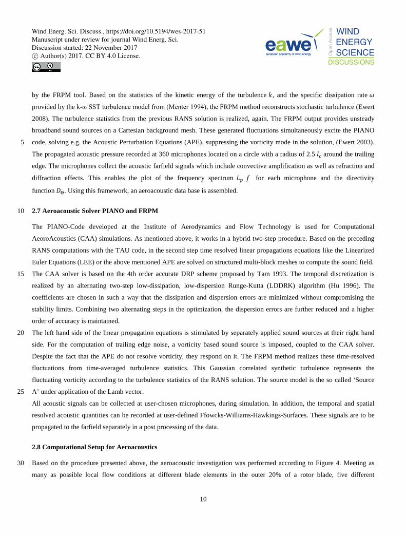
The CFD mesh used for the first step of the hybrid procedure is depicted in Figure 5. In Figure 6 the CAA mesh for the 10
second step is shown. At the trailing edge, the resolution of the small vorticity structures must be realized. The type and
resolution of the meshes were set up according to the best practice from Rautmann 2014. The same holds for the choice of
the computational parameters used for the DLR codes TAU and PIANO.
Figure 5: Unstructured CFD mesh for the aeroacoustic tool chain exemplified for the DU180 consists of 102,500 grid points. The 15 C-topology allows for a resolution of the boundary layer of about 100 prism layers. The mesh extends ±100 𝒍𝒍𝒄𝒄 in the 2D directions.
x/lc
y/l c
0 0.5 1
-0.4
-0.2
0
0.2
0.4
x/lc
y/l c
-100 0 100-100
-50
0
50
100
x/lc
y/l c
0.995 1 1.005 1.01
-0.005
0
0.005
Wind Energ. Sci. Discuss., https://doi.org/10.5194/wes-2017-51Manuscript under review for journal Wind Energ. Sci.Discussion started: 22 November 2017c© Author(s) 2017. CC BY 4.0 License.
12
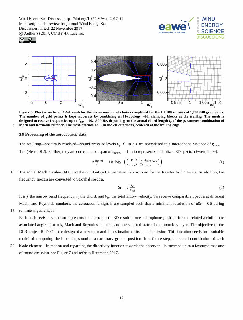
Figure 6: Block-structured CAA mesh for the aeroacoustic tool chain exemplified for the DU180 consists of 1,200,000 grid points. The number of grid points is kept moderate by combining an H-topology with clamping blocks at the trailing. The mesh is designed to resolve frequencies up to fmax = 10…60 kHz, depending on the actual chord length 𝒍𝒍𝒄𝒄 of the parameter combination of Mach and Reynolds number. The mesh extends ±3 𝒍𝒍𝒄𝒄 in the 2D directions, centered at the trailing edge. 5
2.9 Processing of the aeroacoustic data
The resulting—spectrally resolved—sound pressure levels 𝐿𝐿𝑝𝑝(𝑓𝑓) in 2D are normalized to a microphone distance of 𝑟𝑟norm =
1 m (Herr 2012). Further, they are corrected to a span of 𝑠𝑠norm = 1 m to represent standardized 3D spectra (Ewert, 2009).
∆𝐿𝐿𝑝𝑝norm = 10 log10 ��𝑟𝑟
𝑟𝑟norm� � 𝜁𝜁
2𝜋𝜋𝑠𝑠norm𝑟𝑟norm
Ma�� (1)
The actual Mach number (Ma) and the constant ζ=1.4 are taken into account for the transfer to 3D levels. In addition, the 10
frequency spectra are converted to Strouhal spectra.
Sr = 𝑓𝑓 𝑙𝑙𝑐𝑐𝑉𝑉rel
(2)
It is 𝑓𝑓 the narrow band frequency, 𝑙𝑙𝑐𝑐 the chord, and 𝑉𝑉rel the total inflow velocity. To receive comparable Spectra at different
Mach- and Reynolds numbers, the aeroacoustic signals are sampled such that a minimum resolution of ΔSr = 0.5 during
runtime is guaranteed. 15
Each such revised spectrum represents the aeroacoustic 3D result at one microphone position for the related airfoil at the
associated angle of attack, Mach and Reynolds number, and the selected state of the boundary layer. The objective of the
DLR project RoDeO is the design of a new rotor and the estimation of its sound emission. This intention needs for a suitable
model of computing the incoming sound at an arbitrary ground position. In a future step, the sound contribution of each
blade element—in motion and regarding the directivity function towards the observer—is summed up to a favoured measure 20
of sound emission, see Figure 7 and refer to Rautmann 2017.
x/lc
y/l c
0 0.5 1
-0.4
-0.2
0
0.2
0.4
x/lc
y/l c
0.995 1 1.005 1.01
-0.005
0
0.005
x/lc
y/l c
-2 0 2 4
-2
0
2
Wind Energ. Sci. Discuss., https://doi.org/10.5194/wes-2017-51Manuscript under review for journal Wind Energ. Sci.Discussion started: 22 November 2017c© Author(s) 2017. CC BY 4.0 License.
13
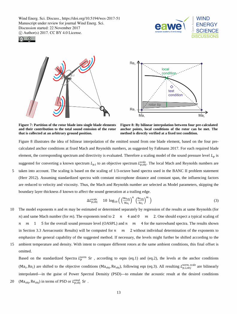
Figure 7: Partition of the rotor blade into single blade elements and their contribution to the total sound emission of the rotor that is collected at an arbitrary ground position.
Figure 8: By bilinear interpolation between four pre-calculated anchor points, local conditions of the rotor can be met. The method is directly verified at a fixed test condition.
Figure 8 illustrates the idea of bilinear interpolation of the emitted sound from one blade element, based on the four pre-
calculated anchor conditions at fixed Mach and Reynolds numbers, as suggested by Faßmann 2017. For each required blade
element, the corresponding spectrum and directivity is evaluated. Therefore a scaling model of the sound pressure level 𝐿𝐿𝑝𝑝 is
suggested for converting a known spectrum 𝐿𝐿𝑝𝑝,𝑖𝑖 to an objective spectrum 𝐿𝐿𝑝𝑝,objscale . The local Mach and Reynolds numbers are
taken into account. The scaling is based on the scaling of 1/3-octave band spectra used in the BANC II problem statement 5
(Herr 2012). Assuming standardized spectra with constant microphone distance and constant span, the influencing factors
are reduced to velocity and viscosity. Thus, the Mach and Reynolds number are selected as Model parameters, skipping the
boundary layer thickness 𝛿𝛿 known to affect the sound generation at a trailing edge.
∆𝐿𝐿𝑝𝑝,objscale = 10 log10 � �Maobj
Ma𝑖𝑖�𝑛𝑛
�Reobj
Re𝑖𝑖�𝑙𝑙
� (3)
The model exponents 𝑛𝑛 and 𝑚𝑚 may be estimated or determined separately by regression of the results at same Reynolds (for 10
𝑛𝑛) and same Mach number (for 𝑚𝑚). The exponents tend to 2 < 𝑛𝑛 < 4 and 0 < 𝑚𝑚 < 2. One should expect a typical scaling of
𝑛𝑛 + 𝑚𝑚 + 1 = 5 for the overall sound pressure level (OASPL) and 𝑛𝑛 + 𝑚𝑚 = 4 for the narrowband spectra. The results shown
in Section 3.3 Aeroacoustic Results) will be computed for 𝑛𝑛 = 𝑚𝑚 = 2 without individual determination of the exponents to
emphasize the general capability of the suggested method. If necessary, the levels might further be shifted according to the
ambient temperature and density. With intent to compare different rotors at the same ambient conditions, this final offset is 15
omitted.
Based on the standardized Spectra 𝐿𝐿𝑝𝑝norm(Sr) , according to eqns (eq.1) and (eq.2), the levels at the anchor conditions
(Ma𝑖𝑖, Re𝑖𝑖) are shifted to the objective conditions (Maobj, Reobj), following eqn (eq.3). All resulting 𝐿𝐿𝑝𝑝,𝑖𝑖,𝑝𝑝𝑜𝑜𝑗𝑗norm, scale are bilinearly
interpolated—in the guise of Power Spectral Densitiy (PSD)—to emulate the acoustic result at the desired conditions
(Maobj, Reobj) in terms of PSD or 𝐿𝐿𝑝𝑝,objemul (Sr). 20
Wind Energ. Sci. Discuss., https://doi.org/10.5194/wes-2017-51Manuscript under review for journal Wind Energ. Sci.Discussion started: 22 November 2017c© Author(s) 2017. CC BY 4.0 License.
14
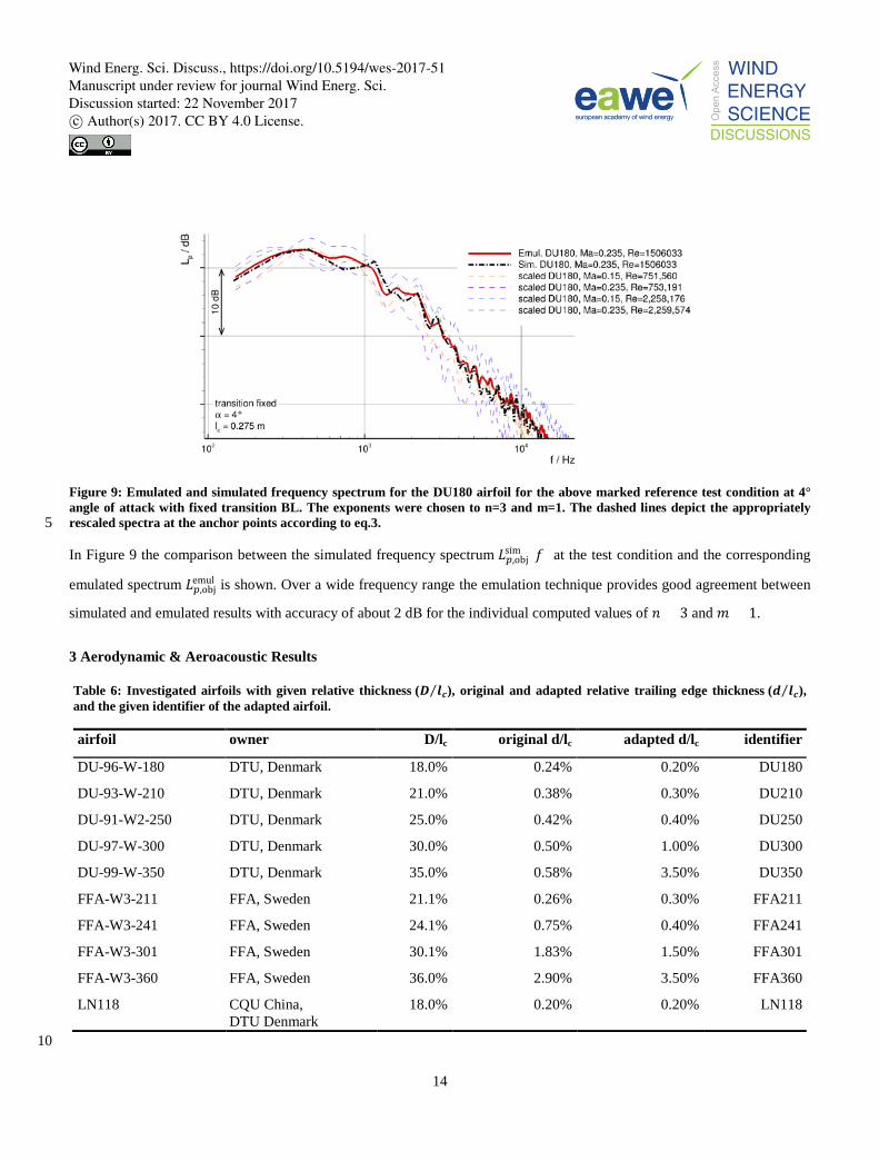
Figure 9: Emulated and simulated frequency spectrum for the DU180 airfoil for the above marked reference test condition at 4° angle of attack with fixed transition BL. The exponents were chosen to n=3 and m=1. The dashed lines depict the appropriately rescaled spectra at the anchor points according to eq.3. 5
In Figure 9 the comparison between the simulated frequency spectrum 𝐿𝐿𝑝𝑝,objsim (𝑓𝑓) at the test condition and the corresponding
emulated spectrum 𝐿𝐿𝑝𝑝,objemul is shown. Over a wide frequency range the emulation technique provides good agreement between
simulated and emulated results with accuracy of about 2 dB for the individual computed values of 𝑛𝑛 = 3 and 𝑚𝑚 = 1.
3 Aerodynamic & Aeroacoustic Results
Table 6: Investigated airfoils with given relative thickness (𝑫𝑫 𝒍𝒍𝒄𝒄⁄ ), original and adapted relative trailing edge thickness (𝒅𝒅 𝒍𝒍𝒄𝒄⁄ ), and the given identifier of the adapted airfoil.
airfoil owner D/lc original d/lc adapted d/lc identifier
DU-96-W-180 DTU, Denmark 18.0% 0.24% 0.20% DU180
DU-93-W-210 DTU, Denmark 21.0% 0.38% 0.30% DU210
DU-91-W2-250 DTU, Denmark 25.0% 0.42% 0.40% DU250
DU-97-W-300 DTU, Denmark 30.0% 0.50% 1.00% DU300
DU-99-W-350 DTU, Denmark 35.0% 0.58% 3.50% DU350
FFA-W3-211 FFA, Sweden 21.1% 0.26% 0.30% FFA211
FFA-W3-241 FFA, Sweden 24.1% 0.75% 0.40% FFA241
FFA-W3-301 FFA, Sweden 30.1% 1.83% 1.50% FFA301
FFA-W3-360 FFA, Sweden 36.0% 2.90% 3.50% FFA360
LN118 CQU China, DTU Denmark
18.0% 0.20% 0.20% LN118
10
Wind Energ. Sci. Discuss., https://doi.org/10.5194/wes-2017-51Manuscript under review for journal Wind Energ. Sci.Discussion started: 22 November 2017c© Author(s) 2017. CC BY 4.0 License.
15
One important goal of this paper is the comparison of aeracoustic characteristics among different airfoils of equivalent
thickness. Because the relative trailing edge thickness (𝑑𝑑 𝑙𝑙𝑐𝑐⁄ ) is one of the key parameters for trailing edge noise, the original
airfoil geometries had to be slightly adapted in order for airfoils of the same thickness to be directly comparable. The
simulated airfoils and its modifications are displayed in Table 6. In the case of validation the original geometry has been
used. Thus the complete airfoil identifier (e.g. DU-97-W-300) has been employed for captions and in the text. On the other 5
hand the short identifier always indicates that for the underlying investigation the modified airfoil has been applied.
3.1 Validation of Aerodynamic Approach
Since the computation of airfoil polars in the post-stall region is a non-trivial task, it is mandatory to validate the proposed
method before starting the computations for the airfoil catalogue. That means that the available methods have to be
compared exemplarily to experimental data. In this case the various available methods will be compared to the experimental 10
data of the well-known DU-93-W-210 and the DU-97-W-300 airfoil. W.A. Timmer from the Technical University of Delft
kindly provided the data for this purpose. Figure 10, Figure 14 and Figure 15 depict the lift, drag and moment coefficient
over the angle of attack of the DU-93-W-210. Besides the experimental data, three CFD computations with different
numerical settings and data obtained from an XFOIL computation are shown. Below and throughout the paper the three
different methods will be termed as: Method 1 (C-topology mesh + k-ω SST or only SST), Method 2 (O-topology mesh + k-15
ω SST) and Method 3 (O-topology mesh + SA negative or only SA).
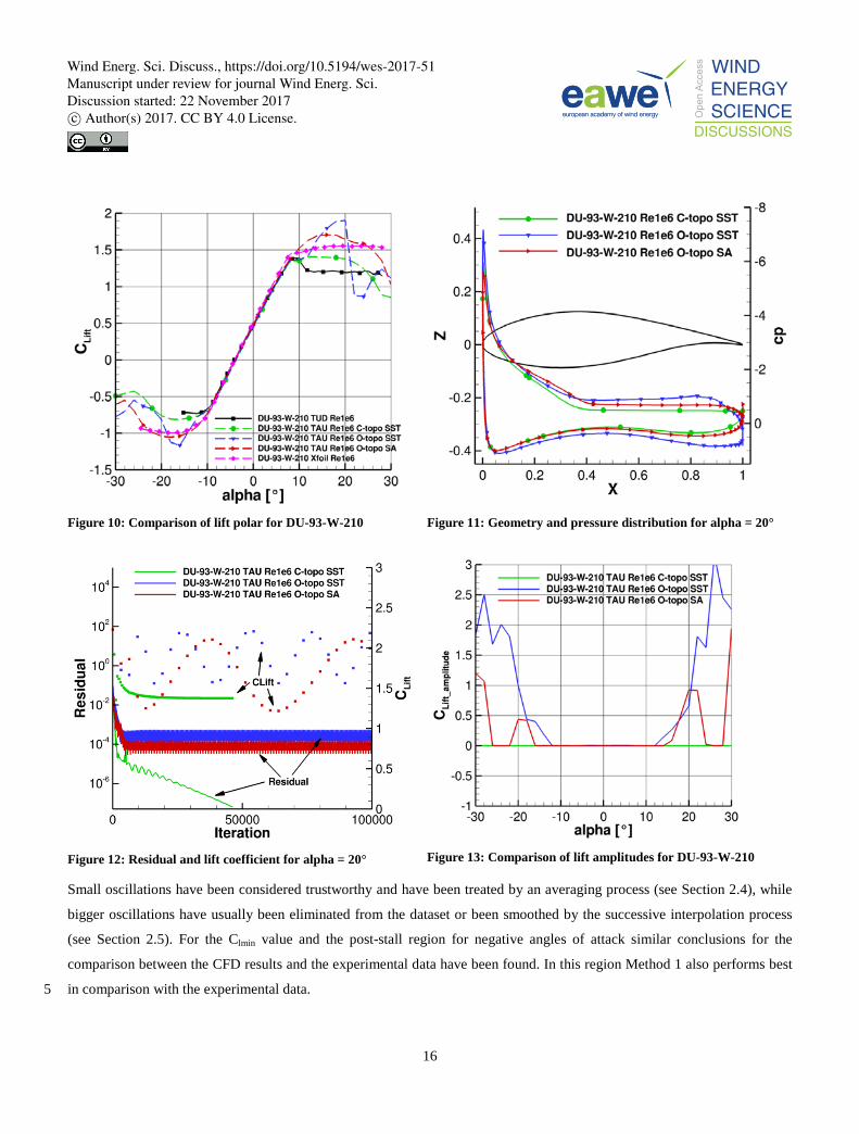
Lift comparison of DU-93-W-210 between -30° and 30° angle of attack (Figure 10):
It can be seen that all methods perform very well in the linear range which extends between -8° and 8° degrees angle of
attack. Major differences occur in the positive and negative stall region. The XFOIL results show hardly any stall behaviour.
The two CFD computations on the O-topology mesh overpredict the Clmax value by 0.3 to 0.5 i.e. 20% and 35% respectively. 20
Only the CFD solution using Method 1 compares very well for Clmax with the experimental value and compares also fairly
well in the post-stall region. The pressure distributions over the airfoil chord are compared in Figure 11. While cP,min is
predicted similarly for Method 1 and 3, the prevision of the suction peak is much higher for Method 2. Subsequently the
results in the region in which the pressure recovery takes place (20% to 40% airfoil chord) differ in that Method 1 predicts a
stronger pressure recovery with the consequence of reaching a smaller underpressure at 40% chord. Even higher differences 25
can be observed on the aft part of the airfoil. The very different pressure distributions are due to a very different prediction of
the trailing edge vortex which has grown substantially in comparison to lower angles of attack and now covers more than
50% of the airfoil chord. Having a closer look at the convergence and the resulting lift coefficients in form of a time series in
Figure 12 reveals that Method 2 and Method 3 have not converged to a satisfactory level resulting in strong oscillations of
the lift coefficient. This behaviour has been observed to be similar for a vast number of profiles within a certain range of 30
angles of attack. Therefore the amplitude of the lift, drag and moment coefficient has always been computed during the post-
processing and is plotted as shown in Figure 13. The visualization of the amplitudes has thereby been used as a trust
indicator.
Wind Energ. Sci. Discuss., https://doi.org/10.5194/wes-2017-51Manuscript under review for journal Wind Energ. Sci.Discussion started: 22 November 2017c© Author(s) 2017. CC BY 4.0 License.
16
Figure 10: Comparison of lift polar for DU-93-W-210
Figure 11: Geometry and pressure distribution for alpha = 20°
Figure 12: Residual and lift coefficient for alpha = 20°
Figure 13: Comparison of lift amplitudes for DU-93-W-210
Small oscillations have been considered trustworthy and have been treated by an averaging process (see Section 2.4), while
bigger oscillations have usually been eliminated from the dataset or been smoothed by the successive interpolation process
(see Section 2.5). For the Clmin value and the post-stall region for negative angles of attack similar conclusions for the
comparison between the CFD results and the experimental data have been found. In this region Method 1 also performs best
in comparison with the experimental data. 5
Wind Energ. Sci. Discuss., https://doi.org/10.5194/wes-2017-51Manuscript under review for journal Wind Energ. Sci.Discussion started: 22 November 2017c© Author(s) 2017. CC BY 4.0 License.
17
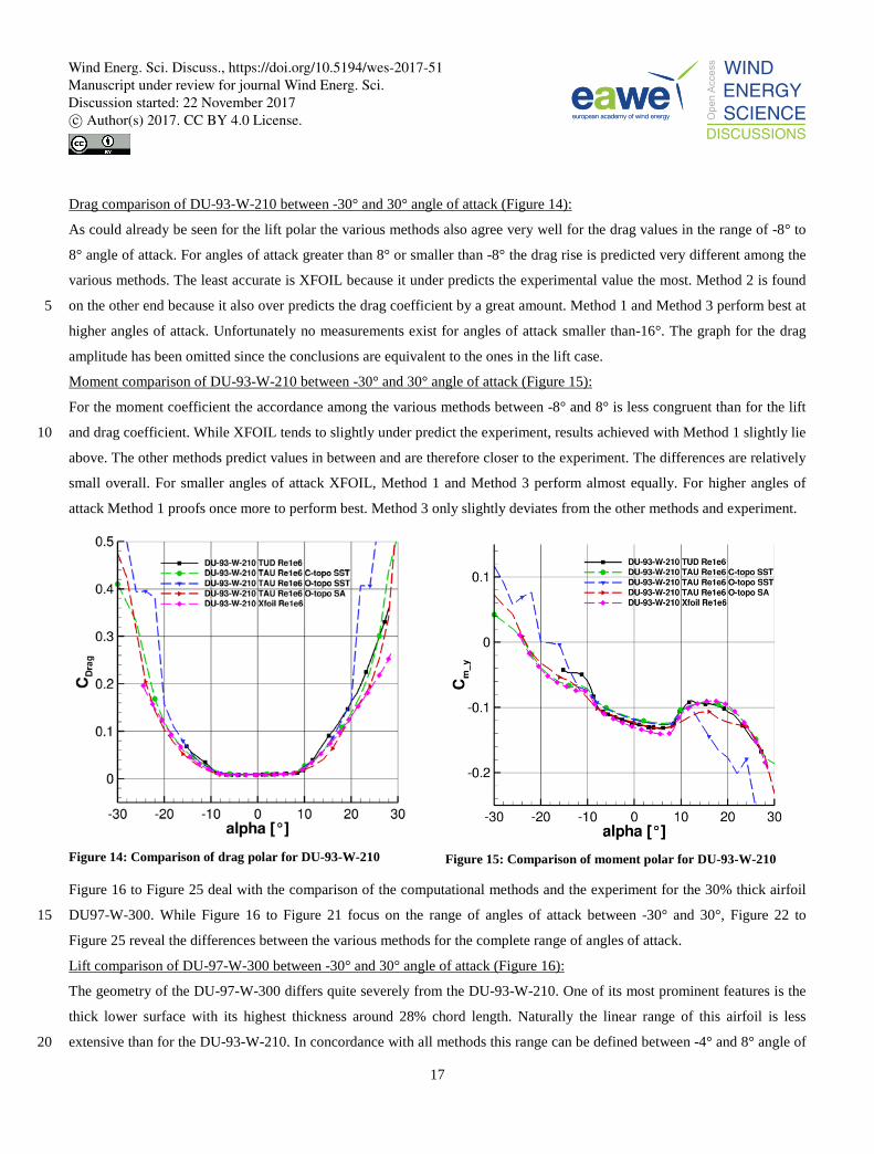
Drag comparison of DU-93-W-210 between -30° and 30° angle of attack (Figure 14):
As could already be seen for the lift polar the various methods also agree very well for the drag values in the range of -8° to
8° angle of attack. For angles of attack greater than 8° or smaller than -8° the drag rise is predicted very different among the
various methods. The least accurate is XFOIL because it under predicts the experimental value the most. Method 2 is found
on the other end because it also over predicts the drag coefficient by a great amount. Method 1 and Method 3 perform best at 5
higher angles of attack. Unfortunately no measurements exist for angles of attack smaller than-16°. The graph for the drag
amplitude has been omitted since the conclusions are equivalent to the ones in the lift case.
Moment comparison of DU-93-W-210 between -30° and 30° angle of attack (Figure 15):
For the moment coefficient the accordance among the various methods between -8° and 8° is less congruent than for the lift
and drag coefficient. While XFOIL tends to slightly under predict the experiment, results achieved with Method 1 slightly lie 10
above. The other methods predict values in between and are therefore closer to the experiment. The differences are relatively
small overall. For smaller angles of attack XFOIL, Method 1 and Method 3 perform almost equally. For higher angles of
attack Method 1 proofs once more to perform best. Method 3 only slightly deviates from the other methods and experiment.
Figure 14: Comparison of drag polar for DU-93-W-210
Figure 15: Comparison of moment polar for DU-93-W-210
Figure 16 to Figure 25 deal with the comparison of the computational methods and the experiment for the 30% thick airfoil
DU97-W-300. While Figure 16 to Figure 21 focus on the range of angles of attack between -30° and 30°, Figure 22 to 15
Figure 25 reveal the differences between the various methods for the complete range of angles of attack.
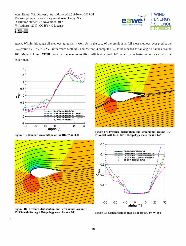
Lift comparison of DU-97-W-300 between -30° and 30° angle of attack (Figure 16):
The geometry of the DU-97-W-300 differs quite severely from the DU-93-W-210. One of its most prominent features is the
thick lower surface with its highest thickness around 28% chord length. Naturally the linear range of this airfoil is less
extensive than for the DU-93-W-210. In concordance with all methods this range can be defined between -4° and 8° angle of 20
Wind Energ. Sci. Discuss., https://doi.org/10.5194/wes-2017-51Manuscript under review for journal Wind Energ. Sci.Discussion started: 22 November 2017c© Author(s) 2017. CC BY 4.0 License.
18
attack. Within this range all methods agree fairly well. As in the case of the previous airfoil most methods over predict the
Clmax value by 15% to 30%. Furthermore Method 2 and Method 3 compute Clmax to be reached for an angle of attack around
16°. Method 1 and XFOIL localize the maximum lift coefficient around 14° which is in better accordance with the
experiment.
Figure 16: Comparison of lift polar for DU-97-W-300
Figure 17: Pressure distribution and streamlines around DU-97-W-300 with k-ω SST + C-topology mesh for α = 14°
Figure 18: Pressure distribution and streamlines around DU-97-300 with SA neg + O-topology mesh for α = 14°
Figure 19: Comparison of drag polar for DU-97-W-300
5
Wind Energ. Sci. Discuss., https://doi.org/10.5194/wes-2017-51Manuscript under review for journal Wind Energ. Sci.Discussion started: 22 November 2017c© Author(s) 2017. CC BY 4.0 License.

19
Figure 17 shows the pressure distribution around the airfoil computed with Method 1 for an angle of attack of 14°. The
equivalent plot for Method 3 is provided in Figure 18. While in the case of the k-ω SST model an incipient trailing edge
separation can be seen, the flow is still fully attached in the case of the SA negative model. This is due to the high suction
peak at the nose predicted by the SA negative model. The lower pressure at the nose leads to a stronger acceleration of the
flow on the first 30% of the suction side and consequently to a higher stream wise velocity on the complete upper surface. 5
Therefore the boundary layer stays attached in case of the SA negative model, while it separates shortly before the trailing
edge in case of the k-ω SST model. Hence the Cl for an angle of attack of 14° is predicted about 0.3 higher by Method 3 in
comparison with Method 1. In fact the over prediction of the Clmax by the SA model in regions with adverse pressure
gradients is quite known and various researchers (e.g. Medida 2013) have tried to improve the model for those kinds of
situations. The differences persist for angles of attack greater than αmax. In this case the flow is separated for both models 10
with k-ω SST always predicting a bigger separation area due to the fact that the kinetic energy in the boundary layer as
predicted by the k-ω SST is smaller than with the SA negative model and therefore separates earlier. The difference in the Cl
value stays about the same as for Clmax, but care has to be taken since the convergence of the SA negative model is not
optimal above Clmax as can be seen by the drag amplitude shown in Figure 20. Although for an angle of attack of e.g. α = 20°
the lift coefficient computed with Method 3 matches best the experimental measurements, it must be noted that the 15
measurements are based only on the pressure sensors and that interference effects with the boundary layer from the wind
tunnel wall might affect the measurements to a greater extent than for smaller angles of attack. Unfortunately the exact
procedure for obtaining the experimental values is unknown.
For the region of negative angles of attack also huge differences can be observed. While separation with the SA negative
model begins at an angle of attack of α = -8°, the separation in case of the k-ω SST model starts already for α = -4°. 20
Unfortunately no experimental data exist in this region of the lift curve. For a Reynolds number of 1e6 (not shown here) the
experimental values match best the results obtained by Method 3. But the transition in the experiment has been influenced by
vortex generators. Therefore an exact comparison is difficult to accomplish.
Drag comparison of DU-97-W-300 between -30° and 30° angle of attack (Figure 19):
As in the case of the previous airfoil the methods agree very well in the linear range. For angles of attack greater than 8° 25
Method 1 and Method 3 perform almost equally well. Differences in Cd are only minor, although the drag amplitude depicted
in Figure 20 indicates that the convergence of the computations between 14° and 24° angle of attack is not optimal. As stated
before the amplitude is only an indicator of potential convergence difficulties. Apparently in this case the oscillations are
small and the averaging process seems to be valid.
On the contrary deviations between Method 1 and Method 3 become bigger for negative angles of attack. Especially 30
around -20° angle of attack the drag polar computed with Method 3 features a discontinuous behavior that looks suspicious.
An examination of the drag amplitude in this region (Figure 20) indicates stronger oscillations and therefore a poorer
convergence of each calculation. Although no experimental data is available in this region, the results obtained with
Method 1 seem to be more trustworthy.
Wind Energ. Sci. Discuss., https://doi.org/10.5194/wes-2017-51Manuscript under review for journal Wind Energ. Sci.Discussion started: 22 November 2017c© Author(s) 2017. CC BY 4.0 License.
20
Method 2 and XFOIL show less agreement with the experimental data for both negative and positive angles of attack outside
the linear range.
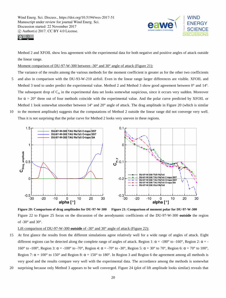
Moment comparison of DU-97-W-300 between -30° and 30° angle of attack (Figure 21):
The variance of the results among the various methods for the moment coefficient is greater as for the other two coefficients
and also in comparison with the DU-93-W-210 airfoil. Even in the linear range larger differences are visible. XFOIL and 5
Method 3 tend to under predict the experimental value. Method 2 and Method 3 show good agreement between 0° and 14°.
The subsequent drop of Cm in the experimental data set looks somewhat suspicious, since it occurs very sudden. Moreover
for α = 20° three out of four methods coincide with the experimental value. And the polar curve predicted by XFOIL or
Method 1 look somewhat smoother between 14° and 20° angle of attack. The drag amplitude in Figure 20 (which is similar
to the moment amplitude) suggests that the computations of Method 2 outside the linear range did not converge very well. 10
Thus it is not surprising that the polar curve for Method 2 looks very uneven in these regions.
Figure 20: Comparison of drag amplitudes for DU-97-W-300
Figure 21: Comparison of moment polar for DU-97-W-300
Figure 22 to Figure 25 focus on the discussion of the aerodynamic coefficients of the DU-97-W-300 outside the region
of -30° and 30°.
Lift comparison of DU-97-W-300 outside of -30° and 30° angle of attack (Figure 22):
At first glance the results from the different simulations agree relatively well for a wide range of angles of attack. Eight 15
different regions can be detected along the complete range of angles of attack. Region 1: α = -180° to -160°, Region 2: α = -
160° to -100°, Region 3: α = -100° to -70°, Region 4: α = -70° to -30°, Region 5: α = 30° to 70°, Region 6: α = 70° to 100°,
Region 7: α = 100° to 150° and Region 8: α = 150° to 180°. In Region 3 and Region 6 the agreement among all methods is
very good and the results compare very well with the experimental data. The accordance among the methods is somewhat
surprising because only Method 3 appears to be well converged. Figure 24 (plot of lift amplitude looks similar) reveals that 20
Wind Energ. Sci. Discuss., https://doi.org/10.5194/wes-2017-51Manuscript under review for journal Wind Energ. Sci.Discussion started: 22 November 2017c© Author(s) 2017. CC BY 4.0 License.

21
Method 1 and Method 2 suffer from severe convergence problems in Region 3 and Region 6. Despite this fact the agreement
is very good. In Region 1 and Region 8 the discrepancies between the methods become greater, but the agreement with the
experimental data is still fair. Especially the results from Method 3 are convincing because the peaks in the experimental
data at various angles of attack (i.e. -164°, -160°, 155°, 165° and 175°) are fairly well captured.
Figure 22: 360° lift polar for DU-97-W-300
Figure 23: 360° drag polar for DU-97-W-300
Figure 24: Comparison of drag amplitudes for DU-97-W-300
Figure 25: 360° moment polar for DU-97-W-300
5
Wind Energ. Sci. Discuss., https://doi.org/10.5194/wes-2017-51Manuscript under review for journal Wind Energ. Sci.Discussion started: 22 November 2017c© Author(s) 2017. CC BY 4.0 License.
22
Less satisfactory are the results from Region 2, Region 4, Region 5 and Region 7. Indeed in these regions the methods
represent the trend of the experimental data fairly well, but they are incapable of matching the absolute value. In average the
predicted value is about 0.3 smaller in comparison to the measured value.
Drag comparison of DU-97-W-300 outside of -30° and 30° angle of attack (Figure 23):
The results with respect to the drag polar are also a bit peculiar. From an examination of Figure 23 Method 1 clearly 5
performs best because the method captures the maximal drag value best. Method 3 stays more than 0.2 below the value
predicted by Method 1. Nevertheless this might also be coincidence because as can be seen from Figure 24 the convergence
of Method 1 outside -30° to 30° is quite unsatisfactory. The second reason why Method 3 is preferred in this area is that the
drag curve is in general smoother than the drag curve computed with Method 1 and especially in comparison with
Method 2.At this point the reader should note that although all methods are not capable of predicting the exact absolute 10
value, all methods predict a smaller drag value for α = -90° than for α = 90°. A feature due to the curvature of the airfoil and
that none of the approximation methods analyzed by Skrzypiński 2014 is able to predict.
Moment comparison of DU-97-W-300 outside of -30° and 30° angle of attack (Figure 25):
Similar as in the case of the drag polar Method 1 seems to obtain the best results for the moment polar as well. On the other
hand Method 3 manages to better capture the kink around -160° and 160°. Nevertheless Method 3 is chosen for further 15
investigations in this area because of its better convergence and in general better smoothness.
As can be seen neither computational approach was superior to all others for all angles of attack. Therefore both
computational setups are used – each setup is applied in the region where it performs best. Afterwards the datasets are fused
to one complete dataset as proposed in Section 2.5 (Interpolation Model for Data Fusion (POT)). 20
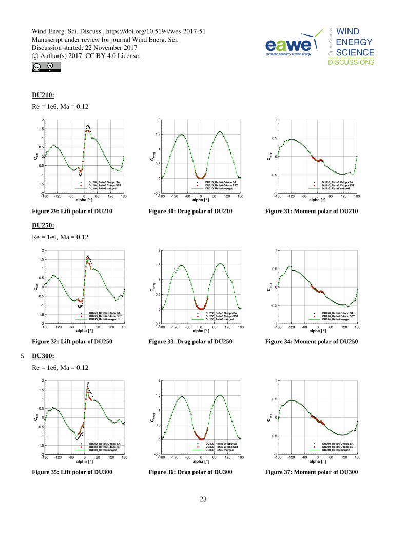
3.2 Aerodynamic Polars
DU180:
Re = 1e6, Ma = 0.12
Figure 26: Lift polar of DU180
Figure 27: Drag polar of DU180
Figure 28: Moment polar of DU180
Wind Energ. Sci. Discuss., https://doi.org/10.5194/wes-2017-51Manuscript under review for journal Wind Energ. Sci.Discussion started: 22 November 2017c© Author(s) 2017. CC BY 4.0 License.
23
DU210:
Re = 1e6, Ma = 0.12
Figure 29: Lift polar of DU210
Figure 30: Drag polar of DU210
Figure 31: Moment polar of DU210
DU250:
Re = 1e6, Ma = 0.12
Figure 32: Lift polar of DU250
Figure 33: Drag polar of DU250
Figure 34: Moment polar of DU250
DU300: 5
Re = 1e6, Ma = 0.12
Figure 35: Lift polar of DU300
Figure 36: Drag polar of DU300
Figure 37: Moment polar of DU300
Wind Energ. Sci. Discuss., https://doi.org/10.5194/wes-2017-51Manuscript under review for journal Wind Energ. Sci.Discussion started: 22 November 2017c© Author(s) 2017. CC BY 4.0 License.
24
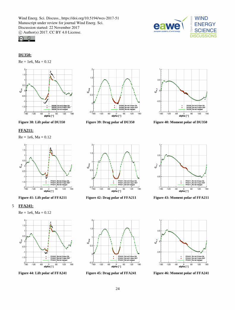
DU350:
Re = 1e6, Ma = 0.12
Figure 38: Lift polar of DU350
Figure 39: Drag polar of DU350
Figure 40: Moment polar of DU350
FFA211:
Re = 1e6, Ma = 0.12
Figure 41: Lift polar of FFA211
Figure 42: Drag polar of FFA211
Figure 43: Moment polar of FFA211
FFA241: 5
Re = 1e6, Ma = 0.12
Figure 44: Lift polar of FFA241
Figure 45: Drag polar of FFA241
Figure 46: Moment polar of FFA241
Wind Energ. Sci. Discuss., https://doi.org/10.5194/wes-2017-51Manuscript under review for journal Wind Energ. Sci.Discussion started: 22 November 2017c© Author(s) 2017. CC BY 4.0 License.
25
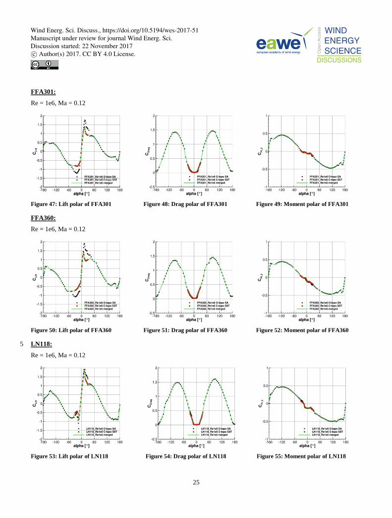
FFA301:
Re = 1e6, Ma = 0.12
Figure 47: Lift polar of FFA301
Figure 48: Drag polar of FFA301
Figure 49: Moment polar of FFA301
FFA360:
Re = 1e6, Ma = 0.12
Figure 50: Lift polar of FFA360
Figure 51: Drag polar of FFA360
Figure 52: Moment polar of FFA360
LN118: 5
Re = 1e6, Ma = 0.12
Figure 53: Lift polar of LN118
Figure 54: Drag polar of LN118
Figure 55: Moment polar of LN118
Wind Energ. Sci. Discuss., https://doi.org/10.5194/wes-2017-51Manuscript under review for journal Wind Energ. Sci.Discussion started: 22 November 2017c© Author(s) 2017. CC BY 4.0 License.
26
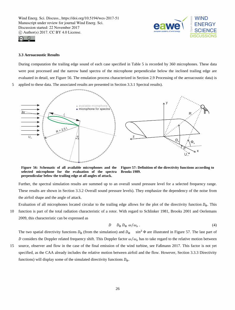
3.3 Aeroacoustic Results
During computation the trailing edge sound of each case specified in Table 5 is recorded by 360 microphones. These data
were post processed and the narrow band spectra of the microphone perpendicular below the inclined trailing edge are
evaluated in detail, see Figure 56. The emulation process characterized in Section 2.9 Processing of the aeroacoustic data) is
applied to these data. The associated results are presented in Section 3.3.1 Spectral results). 5
Figure 56: Schematic of all available microphones and the selected microphone for the evaluation of the spectra perpendicular below the trailing edge at all angles of attack.
Figure 57: Definition of the directivity functions according to Brooks 1989.
Further, the spectral simulation results are summed up to an overall sound pressure level for a selected frequency range.
These results are shown in Section 3.3.2 Overall sound pressure levels). They emphasize the dependency of the noise from
the airfoil shape and the angle of attack.
Evaluation of all microphones located circular to the trailing edge allows for the plot of the directivity function 𝐷𝐷Θ. This
function is part of the total radiation characteristic of a rotor. With regard to Schlinker 1981, Brooks 2001 and Oerlemans 10
2009, this characteristic can be expressed as
𝐷𝐷 = 𝐷𝐷Θ 𝐷𝐷Φ 𝜔𝜔 𝜔𝜔𝑝𝑝⁄ . (4)
The two spatial directivity functions 𝐷𝐷Θ (from the simulation) and 𝐷𝐷Φ = sin2 Φ are illustrated in Figure 57. The last part of
𝐷𝐷 considers the Doppler related frequency shift. This Doppler factor 𝜔𝜔 𝜔𝜔𝑝𝑝⁄ has to take regard to the relative motion between
source, observer and flow in the case of the final emission of the wind turbine, see Faßmann 2017. This factor is not yet 15
specified, as the CAA already includes the relative motion between airfoil and the flow. However, Section 3.3.3 Directivity
functions) will display some of the simulated directivity functions 𝐷𝐷Θ.
Wind Energ. Sci. Discuss., https://doi.org/10.5194/wes-2017-51Manuscript under review for journal Wind Energ. Sci.Discussion started: 22 November 2017c© Author(s) 2017. CC BY 4.0 License.
27
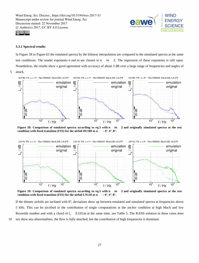
3.3.1 Spectral results
In Figure 58 to Figure 63 the emulated spectra by the bilinear interpolation are compared to the simulated spectra at the same
test conditions. The model exponents 𝑛𝑛 and 𝑚𝑚 are chosen to 𝑛𝑛 = 𝑚𝑚 = 2. The regression of these exponents is still open.
Nonetheless, the results show a good agreement with accuracy of about 3 dB over a large range of frequencies and angles of
attack. 5
Figure 58: Comparison of emulated spectra according to eq.3 with 𝒏𝒏 = 𝒎𝒎 = 𝟐𝟐 and originally simulated spectra at the test condition with fixed transition (FIX) for the airfoil DU180 at 𝜶𝜶 = −𝟒𝟒°,𝟒𝟒°,𝟖𝟖°.
Figure 59: Comparison of emulated spectra according to eq.3 with 𝒏𝒏 = 𝒎𝒎 = 𝟐𝟐 and originally simulated spectra at the test condition with fixed transition (FIX) for the airfoil LN118 at 𝜶𝜶 = −𝟒𝟒°,𝟒𝟒°,𝟖𝟖°.
If the thinner airfoils are inclined with 8°, deviations show up between emulated and simulated spectra at frequencies above
5 kHz. This can be ascribed to the contribution of single computations at the anchor condition at high Mach and low
Reynolds number and with a chord of 𝑙𝑙𝑐𝑐 = 0.101m at the same time, see Table 5. The RANS solution in these cases does
not show any abnormalities, the flow is fully attached, but the contribution of high frequencies is dominant. 10
Wind Energ. Sci. Discuss., https://doi.org/10.5194/wes-2017-51Manuscript under review for journal Wind Energ. Sci.Discussion started: 22 November 2017c© Author(s) 2017. CC BY 4.0 License.
28
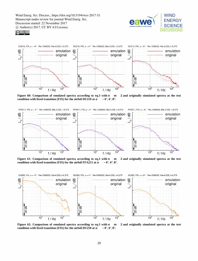
Figure 60: Comparison of emulated spectra according to eq.3 with 𝒏𝒏 = 𝒎𝒎 = 𝟐𝟐 and originally simulated spectra at the test condition with fixed transition (FIX) for the airfoil DU210 at 𝜶𝜶 = −𝟒𝟒°,𝟒𝟒°,𝟖𝟖°.
Figure 61: Comparison of emulated spectra according to eq.3 with 𝒏𝒏 = 𝒎𝒎 = 𝟐𝟐 and originally simulated spectra at the test condition with fixed transition (FIX) for the airfoil FFA211 at 𝜶𝜶 = −𝟒𝟒°,𝟒𝟒°,𝟖𝟖°.
Figure 62: Comparison of emulated spectra according to eq.3 with 𝒏𝒏 = 𝒎𝒎 = 𝟐𝟐 and originally simulated spectra at the test condition with fixed transition (FIX) for the airfoil DU250 at 𝜶𝜶 = −𝟒𝟒°,𝟒𝟒°,𝟖𝟖°.
Wind Energ. Sci. Discuss., https://doi.org/10.5194/wes-2017-51Manuscript under review for journal Wind Energ. Sci.Discussion started: 22 November 2017c© Author(s) 2017. CC BY 4.0 License.
29
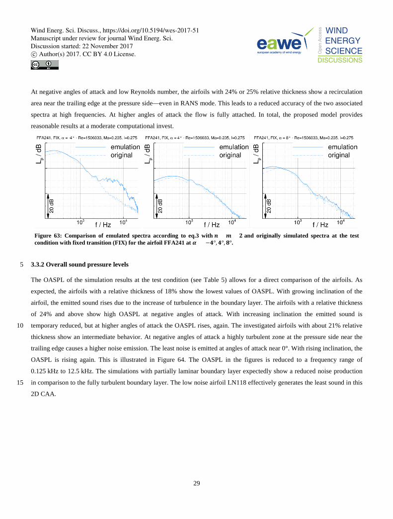
At negative angles of attack and low Reynolds number, the airfoils with 24% or 25% relative thickness show a recirculation
area near the trailing edge at the pressure side—even in RANS mode. This leads to a reduced accuracy of the two associated
spectra at high frequencies. At higher angles of attack the flow is fully attached. In total, the proposed model provides
reasonable results at a moderate computational invest.
Figure 63: Comparison of emulated spectra according to eq.3 with 𝒏𝒏 = 𝒎𝒎 = 𝟐𝟐 and originally simulated spectra at the test condition with fixed transition (FIX) for the airfoil FFA241 at 𝜶𝜶 = −𝟒𝟒°,𝟒𝟒°,𝟖𝟖°.
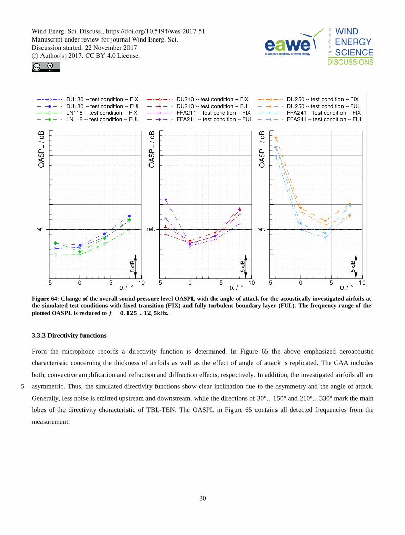
3.3.2 Overall sound pressure levels 5
The OASPL of the simulation results at the test condition (see Table 5) allows for a direct comparison of the airfoils. As
expected, the airfoils with a relative thickness of 18% show the lowest values of OASPL. With growing inclination of the
airfoil, the emitted sound rises due to the increase of turbulence in the boundary layer. The airfoils with a relative thickness
of 24% and above show high OASPL at negative angles of attack. With increasing inclination the emitted sound is
temporary reduced, but at higher angles of attack the OASPL rises, again. The investigated airfoils with about 21% relative 10
thickness show an intermediate behavior. At negative angles of attack a highly turbulent zone at the pressure side near the
trailing edge causes a higher noise emission. The least noise is emitted at angles of attack near 0°. With rising inclination, the
OASPL is rising again. This is illustrated in Figure 64. The OASPL in the figures is reduced to a frequency range of
0.125 kHz to 12.5 kHz. The simulations with partially laminar boundary layer expectedly show a reduced noise production
in comparison to the fully turbulent boundary layer. The low noise airfoil LN118 effectively generates the least sound in this 15
2D CAA.
Wind Energ. Sci. Discuss., https://doi.org/10.5194/wes-2017-51Manuscript under review for journal Wind Energ. Sci.Discussion started: 22 November 2017c© Author(s) 2017. CC BY 4.0 License.
30
Figure 64: Change of the overall sound pressure level OASPL with the angle of attack for the acoustically investigated airfoils at the simulated test conditions with fixed transition (FIX) and fully turbulent boundary layer (FUL). The frequency range of the plotted OASPL is reduced to 𝒇𝒇 = 𝟎𝟎,𝟏𝟏𝟐𝟐𝟏𝟏…𝟏𝟏𝟐𝟐,𝟏𝟏kHz.
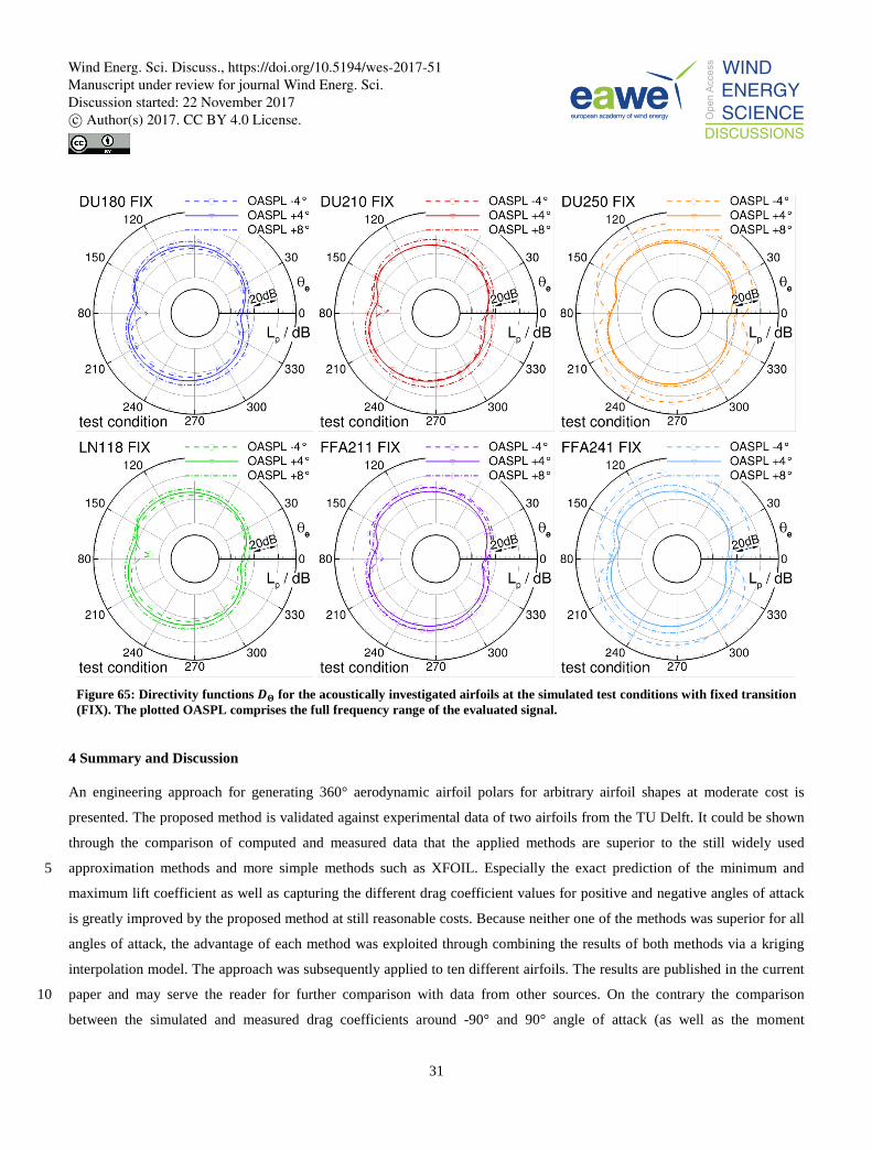
3.3.3 Directivity functions
From the microphone records a directivity function is determined. In Figure 65 the above emphasized aeroacoustic
characteristic concerning the thickness of airfoils as well as the effect of angle of attack is replicated. The CAA includes
both, convective amplification and refraction and diffraction effects, respectively. In addition, the investigated airfoils all are
asymmetric. Thus, the simulated directivity functions show clear inclination due to the asymmetry and the angle of attack. 5
Generally, less noise is emitted upstream and downstream, while the directions of 30°…150° and 210°…330° mark the main
lobes of the directivity characteristic of TBL-TEN. The OASPL in Figure 65 contains all detected frequencies from the
measurement.
Wind Energ. Sci. Discuss., https://doi.org/10.5194/wes-2017-51Manuscript under review for journal Wind Energ. Sci.Discussion started: 22 November 2017c© Author(s) 2017. CC BY 4.0 License.
31
Figure 65: Directivity functions 𝑫𝑫𝚯𝚯 for the acoustically investigated airfoils at the simulated test conditions with fixed transition (FIX). The plotted OASPL comprises the full frequency range of the evaluated signal.
4 Summary and Discussion
An engineering approach for generating 360° aerodynamic airfoil polars for arbitrary airfoil shapes at moderate cost is
presented. The proposed method is validated against experimental data of two airfoils from the TU Delft. It could be shown
through the comparison of computed and measured data that the applied methods are superior to the still widely used
approximation methods and more simple methods such as XFOIL. Especially the exact prediction of the minimum and 5
maximum lift coefficient as well as capturing the different drag coefficient values for positive and negative angles of attack
is greatly improved by the proposed method at still reasonable costs. Because neither one of the methods was superior for all
angles of attack, the advantage of each method was exploited through combining the results of both methods via a kriging
interpolation model. The approach was subsequently applied to ten different airfoils. The results are published in the current
paper and may serve the reader for further comparison with data from other sources. On the contrary the comparison 10
between the simulated and measured drag coefficients around -90° and 90° angle of attack (as well as the moment
Wind Energ. Sci. Discuss., https://doi.org/10.5194/wes-2017-51Manuscript under review for journal Wind Energ. Sci.Discussion started: 22 November 2017c© Author(s) 2017. CC BY 4.0 License.
32
coefficients) reveals that the proposed approach is not optimal within this region. A more sophisticated approach, e.g. a
computation using IDDES as proposed by N. N. Sørensen during the WESC Conference in Copenhagen is needed in order to
determine the exact value for these highly separated flow regions. For the current publication this kind of calculation has not
been considered because it is at least two orders of magnitude more expensive than the proposed approach. To the author’s
opinion a multi-fidelity approach consisting of 2D RANS and more sophisticated computations such as IDDES show a great 5
potential in providing exact results for the complete polar at still justifiable costs.
In the second part of the paper an aeroacoustic method predicting frequency spectra at a target condition was proposed. It
uses pre-calculated anchor conditions and provides reasonable results at moderate costs. The bilinear interpolation of spectra
is based on the assumption that only velocity and viscosity effects affect generation of turbulent boundary-layer trailing-edge
noise (TBL-TEN). The presented level shift is influenced by two model exponents 𝑛𝑛 and 𝑚𝑚. The results show a good 10
agreement between narrow band spectra that are simulated and those that were emulated by the new model with 𝑛𝑛 = 𝑚𝑚 = 2.
In a scheduled contribution to the AIAA/CEAS Aeroacoustic conference in 2018 the exponents will be individually
estimated for each airfoil and angle of attack. The estimation will be performed by regression of level differences at same
Reynolds (for 𝑛𝑛) and same Mach number (for 𝑚𝑚). As shown above, the exponents tend to 2 < 𝑛𝑛 < 4 and 0 < 𝑚𝑚 < 2. One
should expect a typical scaling of 𝑛𝑛 + 𝑚𝑚 + 1 = 5 for the overall sound pressure level (OASPL) and 𝑛𝑛 + 𝑚𝑚 = 4 for the 15
narrowband spectra.
The overall sound pressure level of airfoils with medium relative thickness behaves intermediate in comparison to those with
higher or lower relative thickness. Thus, the blending of angles of attack and different airfoil geometry seems feasible to
meet arbitrary airfoils geometry and flow conditions along the rotor blade.
The quality of the results is dependent on robust RANS simulations. Some combinations of Mach number, Reynolds 20
number, airfoil and angle of attack reveal agile and sensitive behaviour of the flow. This is expected at high angles of attack
were aerodynamic stall is to be due. On the other hand, airfoils with high relative thickness may show highly turbulent areas
near the trailing edge at the pressure side of the airfoils at low or negative angles of attack. To keep the computational effort
as little as possible, these effects are accepted as long as they reflect true physics. The proposed method will provide a good
estimation of the relative levels in a direct comparison of the emitted noise levels of two different rotors, even if single 25
deviating anchor conditions may distort certain emulation spectra. An exact prediction in absolute levels is not the objective,
yet.
The emulated spectra at objective conditions will soon be processed to plot the OASPL and the associated directivity
function in comparison to the simulated ones. This step is a further stage of the verification of the method. During this
ongoing work, the generated data will finally be used to estimate the sound emission at an arbitrary observer position, caused 30
by the respective wind turbine, like illustrated in Figure 7.
Wind Energ. Sci. Discuss., https://doi.org/10.5194/wes-2017-51Manuscript under review for journal Wind Energ. Sci.Discussion started: 22 November 2017c© Author(s) 2017. CC BY 4.0 License.
33
Acknoledgements
The first author expresses his gratitude towards W.A. Timmer from TU Delft for providing the experimental data set of the
two airfoils DU-93-W-210 and DU-97-W-300.
References
Amiet, R.: Acoustic Radiation from an Airfoil in a Turbulent Stream, Journal of Sound and Vibration, Vol. 41, No. 4, 407–5 420, doi 10.1016/S0022-460X(75)80105-2, 1975.
Bangga, G., Kim, Y., Lutz, T., Weihing, P., Krämer, E.: Investigations of the inflow turbulence effect on rotational augmentation by means of CFD, Journal of Physics: Conference Series, 753:1-11, doi10.1088/1742-6596/753/2/022026, 2016.
Brooks, T.F.; Pope, D.S.; Marcolini, M.A.: Airfoil Self-Noise and prediction, NASA Reference Publication 1218, 1989 10
Brooks, T., Burley, C.: Rotor Broadband Noise Prediction with Comparison to Model Data, AIAA/CEAS Aeroacoustics Conference, AIAA 2001-2210, doi10.2514/6.2001-2210, 2001
Drela M., Giles M.: Viscous-Inviscid Analysis of Transonic and Low Reynolds Number Airfoils, AIAA Journal, Vol. 25, No. 10, 1347–1355, doi: 10.2514/3.9789, 1987.
Ewert, R.: Broadband slat noise prediction based on CAA and stochastic sound sources from a fast random particle-mesh 15 (RPM) method, Computers and Fluids vol. 37, No. 4, 369–387, doi: 10.1016/j.compfluid.2007.02.003, 2008
Ewert, R.; Schröder, W.: Acoustic perturbation equations based on flow decomposition via source filtering, Journal of Computational Physics, Vol. 188, No. 2, 365–398, doi: 10.1016/S0021-9991(03)00168-2, 2003
Ewert, R., Appel, C., Dierke, J., Herr, M.: RANS/CAA based prediction of NACA 0012 broadband trailing edge noise and experimental validation, AIAA/CEAS Aeroacoustics Conference, AIAA 2009-3269, doi: 10.2514/6.2009-3269, 2009 20
Faßmann, B., Reiche, N., Ewert, R., Herr, M., Delfs, J.: Aeroacoustic Assessment of Rotor Blades by means of Numerical Methods, German Wind Engergy Conference, DEWEK, Paper submitted, 2017.
Forrester A., Sóbester, A., and Keane, A.: Engineering Design via Surrogate Modelling – A Practical Guide. John Wiley & Sons Ltd., 2008
Gross, A., Fasel, H. F., Friederich, T. and Kloker, M. J.: Numerical investigation of rotational augmentation for S822 wind 25 turbine airfoil, Wind Energy, 15:983-1007, doi:10.1002/we.540, 2012.
Han, Z.-H. and Görtz, S.: A Hierarchical Kriging Model for Variable-Fidelity Surrogate Modeling. In: AIAA Journal 50-9, 1885-1896, 2012.
Herr, M., Bahr, C., Kamruzzaman, M.: Second Workshop on Benchmark Problems for Airframe Noise Computations (BANC-II) – Workshop Category 1: Trailing-Edge Noise, AIAA/CEAS Aeroacoustic Conference, 2012 30
Herr, M., Ewert, R., Rautmann, C., Kamruzzaman, M., Bekiropoulos, D., Iob, A., Arina, R., Batten, P., Chakravarthy, S., Bertagnolio, F.: Broadband Trailing-Edge Noise Predictions - Overview of BANC-III Results. AIAA/CEAS Aeroacoustics Conference, AIAA 2015-2847, doi: 10.2514/6.2015-2847, 2015
Hu, F. Q., Hussaini, M. Y., Manthey, J. L.: Low-dissipation and low-dispersion Runge-Kutta schemes for computational acoustics, Journal of Computational Physics, Vol. 124, No. 1, 177–191, doi: 10.1006/jcph.1996.0052s, 1996. 35
Krumbein, A., Krimmelbein, N., Grabe, C.: Streamline-Based Transition Prediction Techniques in an Unstructured Computational Fluid Dynamics Code, AIAA Journal, Vol. 55, No. 5, pp. 1548 - 1564, DOI: 10.2514/1.J054990, 2017.
Wind Energ. Sci. Discuss., https://doi.org/10.5194/wes-2017-51Manuscript under review for journal Wind Energ. Sci.Discussion started: 22 November 2017c© Author(s) 2017. CC BY 4.0 License.
34
Krumbein, A., Krimmelbein, N., Schrauf, G.: Automatic Transition Prediction in a Hybrid Flow Solver – Part 1: Methodology and Sensitivities, Journal of Aircraft, Vol. 46, No. 4, pp. 1176 - 1190, DOI: 10.2514/1.39736, 2009.
Medida, S., Baeder, J. D.: Adverse Pressure Gradient Modification to Turbulence Models for Wall-bounded Flows, 21st AIAA Computational Fluid Dynamics Conference, doi:10.2514/6.2013-2426, 2013.
Menter, F. R.: Two-equation eddy-viscosity turbulence models for engineering applications, AIAA Journal, Vol. 32, No. 8: 5 1598–1605, doi: 10.2514/3.12149, 1994
Moriarty, P.: NAFNois User’s Manual, National Wind Technology Center, National Renewable Energy Laboratory, 2005
NASA, Turbulence Modeling Resource, https://turbmodels.larc.nasa.gov/naca0012_val_ffeffect.html, 2014.
Ning, S. A.: A simple solution method for the blade element momentum equations with guaranteed convergence, Wind Energy, 17:1327–1345, doi:10.1002/we.1636, 2013. 10
Oerlemans, S., Sijtsma, P., Méndez López, B.: Location and quantification of noise sources on a wind turbine, Journal of Sound and Vibration ,Vol. 299, No. 4-5, doi: 10.1016/j.jsv.2006.07.032, 2007
Oerlemans, S, Fisher, M., Maeder, T., Kögler, K.: Reduction of Wind Turbine Noise Using Optimized Airfoils and Trailing-Edge Serrations, AIAA Journal Vol. 47, No. 6, 1470–1481, doi 10.2514/1.38888, 2009
Parchen R.: Progress report DRAW: A Prediction Scheme for Trailing-Edge Noise Based on Detailed Boundary-Layer 15 Characteristics; TNO Rept. HAG-RPT-980023, TNO Institute of Applied Physics, 1998
Rautmann, C., Dierke, J., Ewert, R., Hu, N., Delfs, J.: Generic Airfoil Trailing-Edge Noise Prediction using Stochastic Sound Sources from Synthetic Turbulence, AIAA/CEAS Aeroacoustics Conference, AIAA 2014-3298, doi: 10.2514/6.2014-3298
Rautmann, C.: Numerical Simulation of Wind Turbine Trailing-Edge Noise, PhD-Thesis, ISSN 1434–8454, 20 ISRN DLR-FB-2017-35, 2017
Schlinker, R. and Amiet, R.: Helicopter Rotor Trailing Edge Noise, NASA Contractor Report 3470, 1981
Schwamborn, D., Gerhold, T. and R. Heinrich: The DLR TAU-Code: Recent Applications in Research and Industry, In proceedings of European Conference on Computational Fluid Dynamics, ECCOMAS CDF, Delft The Netherland, 2006.
Skrzypiński, W., Zahle, F. and Bak, C.: Parametric approximation of airfoil aerodynamic coefficients at high angles of 25 attack, Proceedings of the European Wind Energy Association, 2014.
Snel, H.: Review of Aerodynamics for Wind Turbines, Wind Energy, 6:203–211, doi:10.1002/we.97, 2003.
Tam, C. K. W. and Webb, J. C.: Dispersion-Relation-Preserving Finite Diffrence Schemes for Computational Acoustics, Journal of Computational Physics, Vol. 107, No. 2, 262–281, doi: 10.1006/jcph.1993.1142, 1993
Tangler, J. L. and Kocurek, J. D.: Wind Turbine Post-Stall Airfoil Performance Characteristics Guidelines for Blade-30 Element Momentum Methods, 43rd AIAA Aerospace Sciences Meeting and Exhibit, Reno, Nevada, 2005.
Wagner, S., Bareiß, R., Guidati, G.: Wind Turbine Noise, ISBN 978 0387605920, Springer 1996
Wilke, G.: Variable Fidelity Optimization of Required Power of Rotor Blades: Investigation of Aerodynamic Models and their Application. In: 38th European Rotorcraft Forum, 2012
Wind Energ. Sci. Discuss., https://doi.org/10.5194/wes-2017-51Manuscript under review for journal Wind Energ. Sci.Discussion started: 22 November 2017c© Author(s) 2017. CC BY 4.0 License.