numerical algorithm for polya enumeration theorem´numerical algorithm for polya enumeration...

Numerical Algorithm for Polya Enumeration Theorem

CONRAD W. ROSENBROCK, WILEY S. MORGAN, and GUS L. W. HART,Brigham Young UniversitySTEFANO CURTAROLO, Duke UniversityRODNEY W. FORCADE, Brigham Young University

Although the Polya enumeration theorem has been used extensively for decades, an optimized, purelynumerical algorithm for calculating its coefficients is not readily available. We present such an algorithmfor finding the number of unique colorings of a finite set under the action of a finite group.

Categories and Subject Descriptors: G.2.1 [Discrete Mathematics]: Combinatorics

General Terms: Combinatorial Algorithms, Counting Problems

Additional Key Words and Phrases: Polya enumeration theorem, expansion coefficient, product ofpolynomials

ACM Reference Format:Conrad W. Rosenbrock, Wiley S. Morgan, Gus L. W. Hart, Stefano Curtarolo, and Rodney W. Forcade. 2016.Numerical algorithm for polya enumeration theorem. J. Exp. Algorithmics 21, 1, Article 1.11 (August 2016),17 pages.DOI: http://dx.doi.org/10.1145/2955094

1. INTRODUCTION

A circle partitioned into 4 equal sectors can be colored 16 different ways using twocolors, 24 = 16, as shown in Figure 1. But only 6 of these colorings are symmetricallydistinct, several others being equivalent (under rotations and reflections) as shown bythe arrows in the figure. The Polya enumeration theorem provides a way to determinehow many symmetrically distinct colorings there are with, for example, all sectors red(only one, as shown in the figure), one red sector and three green (again, only one), orthe number with two red sectors and two green sectors (two, as shown in the figure).Borrowing a word from physics and chemistry, we refer to the partition of red andgreen sectors as the stoichiometry. For example, a coloring with 1 red sector and 3green sectors has a stoichiometry of 1:3.

The Polya theorem [Polya 1937; Polya and Read 1987] produces a polynomial (gen-erating function), shown in the figure, whose coefficients answer the question of howmany distinct colorings there are for each stoichiometry (each partition of the colors).For example, the 2r2g2 term in the polynomial indicates that there are two distinctways to color the circle with 2:2 stoichiometry ( ). For all other stoichiometries (4:0,

This work was supported under Grant No. ONR (MURI N00014-13-1-0635).Authors’ addresses: C. W. Rosenbrock, W. S. Morgan, and G. L. W. Hart, Department of Physics and As-tronomy, 84602, Brigham Young University; S. Curtarolo, Materials Science, Electrical Engineering, Physicsand Chemistry, 27708, Duke University; R. W. Forcade, Department of Mathematics, 84602, Brigham YoungUniversity.Permission to make digital or hard copies of part or all of this work for personal or classroom use is grantedwithout fee provided that copies are not made or distributed for profit or commercial advantage and thatcopies show this notice on the first page or initial screen of a display along with the full citation. Copyrights forcomponents of this work owned by others than ACM must be honored. Abstracting with credit is permitted.To copy otherwise, to republish, to post on servers, to redistribute to lists, or to use any component of thiswork in other works requires prior specific permission and/or a fee. Permissions may be requested fromPublications Dept., ACM, Inc., 2 Penn Plaza, Suite 701, New York, NY 10121-0701 USA, fax +1 (212)869-0481, or [email protected]© 2016 ACM 1084-6654/2016/08-ART1.11 $15.00DOI: http://dx.doi.org/10.1145/2955094

ACM Journal of Experimental Algorithmics, Vol. 21, No. 1, Article 1.11, Publication date: August 2016.

http://dx.doi.org/10.1145/2955094

http://dx.doi.org/10.1145/2955094

1.11:2 C. W. Rosenbrock et al.

Fig. 1. Top row: All possible two-color colorings of a circle divided into four equal sectors (left side of figure).Bottom row: All symmetrically distinct binary colorings of the circle. Arrows indicate combinatoricallydistinct colorings that are equivalent by symmetry.

0:4, 1:3, and 3:1), the polynomial coefficients are all 1, indicating that for each of thesecases there is only one distinct coloring, as is obvious from the figure.

A common problem in many fields involves enumerating1 the symmetrically distinctcolorings of a finite set, similar to the toy problem of Figure 1. The Polya theoremhas shown its wide range of applications in a variety of contexts. Classically, it wasapplied to counting chemical isomers [Robinson et al. 1976; Kennedy et al. 1964; Polya1937] and graphs [Harary 1955]. Recent examples include confirming enumerationsof molecules in bioinformatics and chemoinformatics [Deng and Qian 2014; Ghorbaniand Songhori 2014]; unlabeled, uniform hypergraphs in discrete mathematics [Qian2014]; analysis of tone rows in musical composition [Lackner et al. 2015]; commuta-tive binary models of Boolean functions in computer science [Genitrini et al. 2015];generating functions for single-trace-operators in high-energy physics [McGrane et al.2015]; investigating the role of nonlocality in quantum many-body systems [Tura et al.2015]; and photosensitizers in photosynthesis research [Taniguchi et al. 2014].

In computational materials science, chemistry, and related subfields such as compu-tational drug discovery, combinatorial searches are becoming increasingly important,especially in high-throughput studies [Curtarolo et al. 2013]. As computational meth-ods gain a larger market share in materials and drug discovery, algorithms such asthe one presented in this article are important as they provide validation support tocomplex enumeration codes. Polya’s theorem is the only way to independently confirmthat an enumeration algorithm has performed correctly. The present algorithm hasbeen useful in checking a new algorithm extending the work in Hart and Forcade[2008, 2009] and Hart et al. [2012], and Polya’s theorem was recently used in a similarcrystal enumeration algorithm [Mustapha et al. 2013] that has been incorporated intothe CRYSTAL14 software package [Dovesi et al. 2014].

Despite the widespread use of Polya’s theorem in different science and mathematicscontexts, a low-level, numerical implementation is not available. Typical approachesuse Computer Algebra Systems (CASs) to symbolically generate the Polya polynomial.This strategy is ineffective for two reasons. First, CASs are too slow for large problemsthat arise in a research setting, and, second, generating the entire Polya polynomial(which can have billions or trillions of terms) is unnecessary when one is interested inonly a single stoichiometry.

1The Polya theorem does not generate the list of unique colorings (which is generally a much harder problem),but it does determine the number of unique colorings.


Numerical Algorithm for Polya Enumeration Theorem 1.11:3

Here we demonstrate a low-level algorithm for finding the polynomial coefficientcorresponding to a single stoichiometry. It exploits the properties of polynomials and apriori knowledge of the relevant term. We briefly describe the Polya enumeration the-orem in Section 2, followed by the algorithm for calculating the polynomial coefficientsin Section 3. In the final section, we investigate the scaling and performance of thealgorithm.

2. POLYA ENUMERATION THEOREM

2.1. Introduction the Polya Enumeration Theorem

Polya’s theorem provides a simple way to construct a generating polynomial whosecoefficients count the numbers of symmetrically distinct colorings for each possiblestoichiometry. The polynomial in Figure 1 above was easy to verify because we wereable to hand count the symmetrically distinct colorings. But suppose there were dozensof colors and dozens of sites to be colored and hundreds of symmetries to apply. In thatcase, it is easier to use Polya’s theorem to construct the polynomial directly from thesymmetry group.

To describe this very useful theorem, we refer once more to Figure 1. There are foursymmetries—the identity, two 90◦ rotations (clockwise and counterclockwise), and a180◦ rotation. If we label the colorable sectors 1, 2, 3, and 4, and write the permutationsin disjoint-cycle notation, we have (1)(2)(3)(4) for the identity, the two 90◦ rotations arerepresented by (1234) and (1432), while the 180◦ rotation is (13)(24) in cycle notation.

Now Polya’s theorem simply tells us to replace each cycle of length λ with a sum ofλ-th powers of variables corresponding to the colors available. For example, letting rand g stand for red and green, the identity is represented by (r + g)(r + g)(r + g)(r + g),the two 90◦ rotations are each replaced by (r4 +g4), and the 180◦ rotation is replaced by(r2 +g2)(r2 +g2). When we average these four polynomials, we get the Polya polynomialpredicted above:

P(r, g) = 14

((r + g)(r + g)(r + g)(r + g) + (r4 + g4) + (r4 + g4) + (r2 + g2)(r2 + g2)

)= r4 + r3g + 2r2g2 + rg3 + g4.

(1)

In other words, Polya’s theorem relies on a structural representation of the sym-metries as permutations written in disjoint-cycle notation to construct the generatingpolynomial we need.

The problem with Polya, however, is that it requires us to compute the entire poly-nomial when we may need only one of its coefficients. For example, if we have 50 sitesto color, and 20 colors available, the number of terms in our polynomial (regardless ofsymmetries) would be about 4.6 × 1016. That is a lot of work (and memory) to computethe entire polynomial (and all of those very large terms) if we needed only to know thenumber of symmetrically distinct colorings for a single stoichiometry. That informationis contained in just 1 term of the 46 quadrillion terms of the Polya polynomial. Can wespare ourselves the work of computing all the others?

Suppose we have a target stoichiometry [c1 : c2 : · · · : cξ ], where ξ is the numberof colors and

∑ξ

j=1 c j = n is the number of sites to be colored. To find the number ofsymmetrically distinct colorings with those frequencies, we must determine the coef-ficient of the single term in the Polya polynomial containing the product xc1

1 xc22 . . . xcξ

ξ .The Polya polynomial is the average,

P(x1, x2, . . . , xξ ) = 1|G|

(∑π∈G

Pπ (x1, x2, . . . , xξ )

), (2)



of the polynomials Pπ (x1, x2, . . . , xξ ) computed for each permutation π in the symmetrygroup G, each Pπ being formed by multiplying the representations of each disjoint cyclein π (as illustrated in Equation (1)).

Clearly, if we are only interested in the coefficient of xc11 xc2

2 . . . xcξ

ξ in P, we may simplyfind the coefficient of that product in each Pπ and add those partial coefficients together.Thus, given a permutation π with k1 cycles of length r1, k2 cycles of length r2, and soon, up to kt cycles of length rt, with

∑ti=1 riki = n (the number of sites, t is the number

of cycle types), we must compute the coefficient of xc11 xc2

2 . . . xcξ

ξ in Pπ .It is well known that a product of sums is equal to the sum of all products one

can obtain by taking one summand from each factor (generalizing the familiar FirstOuter Inner Last (FOIL) rule used by undergrads to multiply two binomials). Thusthe polynomial Pπ is the sum of all products of the form

∏s xλ(s)

is (where the productruns over all cycles s, λ(s) is the length of the cycle s, and xis is one of the colors chosenfrom the sum for that cycle). Thus the product we want, xc1

1 xc22 . . . xcξ

ξ , has a coefficientthat simply counts the number of products of the form

∏s xλ(s)

is where the sum of theexponents for each xi is equal to the target ci.

Each cycle, of length ri (i = 1 . . . t), gets assigned to one of the colors. Let sij be thenumber of cycles of length ri assigned to color j ( j = 1 . . . ξ ). This defines a t × ξ matrixS = (sij) of non-negative integers, where (1) the sum of row i equals the number ofcycles of length ri:

ξ∑j=1

sij = ki (row sum condition), (3)

and (2) weighted sum of column j must equal the target frequency of the j-th color:t∑

i=1

risij = c j (column sum condition), (4)

in order to achieve our target stoichiometry.For each such matrix, there are a number of possible ways to assign colors to the

cycles, with multiplicities prescribed by S. The number is

F(S) =t∏

i=1

(ki

si1, si2, . . . , siξ

), (5)

the product of the number of ways to do it for each cycle. Thus we are obliged to sumthe function F(S), so computed, over all matrices S meeting the given row and columnsum conditions (3) and (4).

If we do this computation for each permutation π , and average them (add themand divide by |G|), we then get the coefficient of the Polya polynomial P(x1, x2, . . . , xi)corresponding to our target stoichiometry [c1 : c2 : · · · : cξ ]. This calculation dependsonly on the cycle type of the permutation, the number of disjoint cycles of differentlengths comprising the disjoint-cycle representation. Thus we only need to make aninventory of the cycle types for our permutations and do the calculation once for eachdistinct cycle type. There will not be more such cycle types than the number of conjugacyclasses in the symmetry group. Also, note, the utility of multinomial coefficients in thiscontext stems from the likelihood that our permutations will have many cycles of thesame length.

Algorithmically, the process is straight forward. First, we must find all matrices Swhich meet the row and sum conditions (3) and (4) above. For each successful matrix,



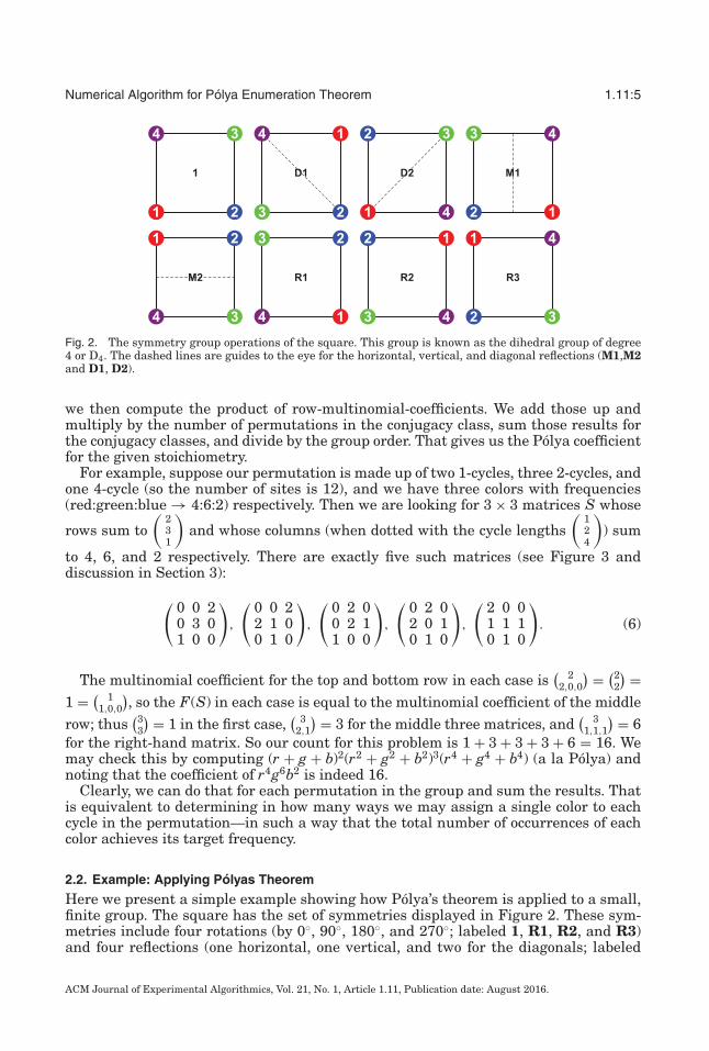
Fig. 2. The symmetry group operations of the square. This group is known as the dihedral group of degree4 or D4. The dashed lines are guides to the eye for the horizontal, vertical, and diagonal reflections (M1,M2and D1, D2).

we then compute the product of row-multinomial-coefficients. We add those up andmultiply by the number of permutations in the conjugacy class, sum those results forthe conjugacy classes, and divide by the group order. That gives us the Polya coefficientfor the given stoichiometry.

For example, suppose our permutation is made up of two 1-cycles, three 2-cycles, andone 4-cycle (so the number of sites is 12), and we have three colors with frequencies(red:green:blue → 4:6:2) respectively. Then we are looking for 3 × 3 matrices S whose

rows sum to(

231

)and whose columns (when dotted with the cycle lengths

(124

)) sum

to 4, 6, and 2 respectively. There are exactly five such matrices (see Figure 3 anddiscussion in Section 3):

( 0 0 20 3 01 0 0

),

( 0 0 22 1 00 1 0

),

( 0 2 00 2 11 0 0

),

( 0 2 02 0 10 1 0

),

( 2 0 01 1 10 1 0

). (6)

The multinomial coefficient for the top and bottom row in each case is( 2

2,0,0

) = (22

) =1 = ( 1

1,0,0

), so the F(S) in each case is equal to the multinomial coefficient of the middle

row; thus(3

3

) = 1 in the first case,( 3

2,1

) = 3 for the middle three matrices, and( 3

1,1,1

) = 6for the right-hand matrix. So our count for this problem is 1 + 3 + 3 + 3 + 6 = 16. Wemay check this by computing (r + g + b)2(r2 + g2 + b2)3(r4 + g4 + b4) (a la Polya) andnoting that the coefficient of r4g6b2 is indeed 16.

Clearly, we can do that for each permutation in the group and sum the results. Thatis equivalent to determining in how many ways we may assign a single color to eachcycle in the permutation—in such a way that the total number of occurrences of eachcolor achieves its target frequency.

2.2. Example: Applying Polyas Theorem

Here we present a simple example showing how Polya’s theorem is applied to a small,finite group. The square has the set of symmetries displayed in Figure 2. These sym-metries include four rotations (by 0◦, 90◦, 180◦, and 270◦; labeled 1, R1, R2, and R3)and four reflections (one horizontal, one vertical, and two for the diagonals; labeled



Table I. Disjoint-Cyclic Form for Each Group Operation in D4 and the CorrespondingPolynomials, Expanded Polynomials and the Coefficient of the x2y2 Term for Each

Op. Disjoint-Cyclic Polynomial Expanded Coeff.

1 (1)(2)(3)(4) (x + y)4 x4 + 4x3 y + 6x2 y2 + 4xy3 + y4 6

D1 (1, 3)(2)(4) (x2 + y2)(x + y)2 x4 + 2x3 y + 2x2 y2 + 2xy3 + y4 2

D2 (1)(2, 4)(3) (x2 + y2)(x + y)2 x4 + 2x3 y + 2x2 y2 + 2xy3 + y4 2

M1 (1, 2)(3, 4) (x2 + y2)2 x4 + 2x2 y2 + y4 2

M2 (1, 4)(2, 3) (x2 + y2)2 x4 + 2x2 y2 + y4 2

R1 (1, 4, 3, 2) (x4 + y4) x4 + +y4 0

R2 (1, 3)(2, 4) (x2 + y2)2 x4 + 2x2 y2 + y4 2

R3 (1, 2, 3, 4) (x4 + y4) x4 + +y4 0

M1, M2 and D1, D2). This group is commonly known as the dihedral group of degreefour, or D4 for short.2

The group operations of the D4 group can be written in disjoint-cyclic form as inTable I. For each r-cycle in the group, we can write a polynomial in variables xr

i fori = 1 . . . ξ , where ξ is the number of colors used. For this example, we will consider thesituation where we want to color the four corners of the square with only two colors. Inthat case we end up with just two variables x1, x2, which are represented as x, y in thetable.

The Polya representation for a single group operation in disjoint-cyclic form resultsin a product of polynomials that we can expand. For example, the group operation D1has disjoint-cyclic form (1, 3)(2)(4) that can be represented by the polynomial (x2 +y2)(x + y)(x + y), where the exponent on each variable corresponds to the length of ther-cycle of which it is a part. For a general r-cycle, the polynomial takes the form(

xr1 + xr

2 + · · · + xrξ

), (7)

for an enumeration with ξ colors. As described in Section 2.1, we exchange the groupoperations acting on the set for polynomial representations that obey the familiar rulesfor polynomials.

We will now pursue our example of the possible colorings on the four corners of thesquare involving two of each color. Excluding the symmetry operations, we could comeup with

(42

) = 6 possibilities, but some of these are equivalent by symmetry. The Polyatheorem counts how many unique colorings we should recover. To find that number, welook at the coefficient of the term corresponding to the overall color selection (in thisexample, two of each color); thus we look for coefficients of the x2y2 term for each groupoperation. These coefficient values are listed in Table I. The sum of these coefficients,divided by the number of operations in the group, gives the total number of uniquecolorings under the entire group action, in this case (6 + 2 + 2 + 2 + 2 + 0 + 2 + 0)/8 =16/8 = 2.

Next, we apply the procedure discussed in connection with Equation (6) to constructthe matrix S for one of the permutations of the square. It illustrates the idea behindthe general algorithm presented in the next section.

In the symmetries of the square, there is a cycle type consisting of two 1-cycles andone 2-cycle. The two permutations with that type are (1)(3)(24) and (2)(4)(13). Thecycle lengths are 1 (with multiplicity 2) and 2 (with multiplicity 1). So each of those

2The dihedral groups have multiple, equivalent names. D4 is also called Dih4 or the dihedral group of order8 (D8).



permutations requires a matrix S =(

s11s21

s12s22

)satisfying s11 + s12 = 2 and s21 + s22 = 1

(row sum condition (3)) and s11 + 2s21 = 2 and s12 + 2s22 = 2 (column sum condition(4)). There are only two matrices of non-negative integers satisfying those conditionssimultaneously: (

2 00 1

)and

(0 21 0

). (8)

For each of these matrices, the row-multinomial coefficients are( 2

0,2

) = 1 and( 1

0,1

) = 1so each matrix yields a product 1. Thus each permutation of this cycle type contributes2 to the sum. This corresponds to the fact that the coefficient of x2y2 in (x + y)2(x2 + y2)is 2.

Since there are two permutations of this cycle type, the total contribution of the cycletype to the overall Polya polynomial is 4 (which must then be divided by the numberof symmetries in the group).

Thus, in general, the only problem is to find an efficient way of generating these ma-trix solutions. Since the problem is equivalent to enumerating all lattice points withina high-dimensional polytope, we presume that a tree search (implemented recursivelyor via a backtracking algorithm) may be the most efficient way to achieve this.

3. COEFFICIENT-FINDING ALGORITHM

Our implementation of the tree search is fundamentally identical to the method of thelast section; however, the details may not be immediately recognizable as such.3 Inthis section we rephrase the row and column sum conditions (3) and (4) to highlightthe logical connections between our specific implementation and the general ideasfrom Section 2. We adopt this approach because (1) for pedagogical value, the matrixapproach is much easier to visualize and (2) the algorithms presented here mirror theaccompanying code closely, which we consider valuable.

First, for a generic polynomial

(xr

1 + xr2 + · · · + xr

ξ

)d, (9)

the exponents of each xi in the expanded polynomial are constrained to the set

V = {0, r, 2r, 3r, . . . , dr}. (10)

Next, we consider the terms in the expansion of the polynomial:

(xr

1 + xr2 + · · · + xr

ξ

)d =∑

k1,k2,...,kξ

μk

ξ∏i=1

xrkii , (11)

where the sum is over all possibles sequences k1, k2, . . . , kξ such that the sum of theexponents (represented by the sequence in ki) is equal to d,

k1 + k2 + · · · + kξ = d. (12)

3If all you are looking for is a working code, you now know enough to use it. Download it at https://github.com/rosenbrockc/polya.



As described in the introduction, the coefficients μk in the polynomial expansionEquation (11) are found using the multinomial coefficients

μk =(

nk1, k2, . . . , kξ

)= n!

k1!k2! · · · kξ !

=(

k1

k1

)(k1 + k2

k2

)· · ·

(k1 + k2 + · · · + kξ

kξ

)

=ξ∏

i=1

(∑ij=1 kj

ki

). (13)

Finally, we define the polynomial (7) for an arbitrary group operation π ∈ G as4

Pπ (x1, x2, . . . , xξ ) =m∏

α=1

Mrα

α (x1, x2, . . . , xξ ), (14)

where each Mrαα is a polynomial of the form (9) for the αth distinct r-cycle and dα is the

multiplicity of that r-cycle; m is the number of cycle types in Pπ . Linking back to thematrix formulation, each Mrα

α is equivalent to a row Si in matrix S.Since we know the fixed stoichiometry term T = ∏ξ

i=1 Ti = ∏ξ

i=1 xcii in advance, we

can limit the possible sequences of ki for which multinomial coefficients are calculated.This is the key idea of the algorithm and the reason for its high performance.

For each group operation π , we have a product of polynomials Mrαα . We begin filtering

the sequences by choosing only those combinations of values viα ∈ Vα = {viα}dα+1i=1 for

which the summ∑

α=1

viα = Ti, (15)

where Vα is the set from Eq. (10) for multinomial Mrαα . At this point it is useful to refer

to Figure 3 to make the connection to the recursive tree search for possible matrices.The Vα are equivalent to all the possible values that any of the elements in a row of thematrix may take. If we take Mr1

1 as an example, then V1 is the collection of all valuesthat show up in row 1 of any matrix in the figure, multiplied by the number of cycleswith length r1. Constraint (15) is equivalent to the column sum requirement (4).

We first apply constraint (15) to the x1 term across the product of polynomials to finda set of values {k1α}m

α=1 that could give exponent T1 once all the polynomials’ terms havebeen expanded. This is equivalent to finding the set of first columns in each matrixthat match the target frequency for the first color. Once a value k1α has been fixed foreach Mrα

α , the remaining exponents in the sequence {k1α} ∪ {kiα}ξi=2 are constrained via(12). We can recursively examine each variable xi in turn using these constraints tobuild a set of sequences

Sl = {Slα}mα=1 = {(k1α, k2α, . . . , kξα)}m

α=1, (16)

where each Slα defines the exponent sequence for its polynomial Mrαα that will produce

the target term T after the product is expanded. Each Slα ∈ Sl represents the trans-posed matrix S that survives both the row and column sum conditions (highlighted ingreen in the figure). Thus, Sl is the set of these matrices for the group operation π . The

4We will use Greek subscripts to label the polynomials in the product and Latin subscripts to label thevariables within any of the polynomials.



Fig. 3. A recursive tree search for some of the possible matrices S for the problem of Section 2: two 1-cycles,three 2-cycles, and one 4-cycle. We have restricted the figure to include only the zero pendants of the tree,which produce four of the five relevant matrices in Equation (6). Matrix elements in red (blue) represent theonly possible values that would satisfy the row (column) sum conditions. A red (blue) cross over a matrixshows that it fails the row (column) sum condition, and its descendants need not be examined. Matrices withgreen borders are solutions to the tree search problem. The purple squares show the current row and columnon which the recursive search is operating.

maximum value of l depends on the target term T and how many possible viα valuesare filtered out using constraints (15) and (12) at each step in the recursion.

Once the set S = {Sl} has been constructed, we use Equation (13) on each polynomial’s{kiα}ξi=1 in Slα to find the contributing coefficients. The final coefficient value for termT resulting from group operation π is

tπ =∑

l

τl =∑

l

m∏α=1

(dα

Slα

). (17)

To find the total number of unique colorings under the group action, this process isapplied to each element π ∈ G and the results are summed and then divided by |G|.

We can further optimize the search for contributing terms by ordering the exponentsin the target term T in descending order. All the {k1α}m

α=1 need to sum to T1 (15); largervalues for T1 are more likely to result in smaller sets of {kiα}m

α=1 across the polynomials.This happens because if T1 has smaller values (like 1 or 2), then we end up withlots of possible ways to arrange them to sum to T1 (which is not the the case for thelarger values). Since the final set of sequences Sl is formed using a Cartesian product,including a few extra sequences from any Ti prunings multiplies the total number of



sequences significantly. In the figure, this optimization is equivalent to completing arow with red entries because all the remaining, unfilled entries are constrained by therow sum condition.

Additionally, constraint (12) applied within each polynomial will also reduce thetotal number of sequences to consider if the first variables x1, x2, and so on, are largerintegers compared to the target values T1, T2, and so on. This speed-up comes fromthe recursive implementation: If x1 is already too large (compared to T1), then possiblevalues for x2, x3, . . . are never considered. This optimization is equivalent to completingmatrix columns with blue entries because of the column sum constraint.

3.1. Pseudocode Implementation

Note: Implementations in PYTHON and FORTRAN are available in the supplementarymaterial.

For both algorithms presented below, the operator (⇐) pushes the value to its rightonto the list to its left.

For algorithm (1) in the EXPAND procedure, the ∪ operator horizontally concatenatesthe integer root to an existing sequence of integers.

For BUILD_Sl, we use the exponent k1α on the first variable in each polynomial toconstruct a full set of possible sequences for that polynomial. Those sets of sequencesare then combined in SUM_SEQUENCES (alg. 2) using a Cartesian product over the sets ineach multinomial.

When calculating multinomial coefficients, we use the form in Eq. (13) in terms ofbinomial coefficients with a fast, stable algorithm from Manolopoulos [2002].

In practice, many of the group operations π produce identical productsMr1

1 Mr22 . . . Mrm

m . Thus before computing any of the coefficients from the polynomials,we first form the polynomial products for each group operation and then add identicalproducts together.

4. COMPUTATIONAL ORDER AND PERFORMANCE

The algorithm is structured around the a priori knowledge of the target stoichiometry.At the earliest possibility, we prune terms from individual polynomials that wouldnot contribute to the final Polya coefficient in the expanded product of polynomials(see Figure 3). Because the Polya polynomial for each group operation is based on itsdisjoint-cyclic form, the complexity of the search can vary drastically from one groupoperation to the next. That said, it is common for groups to have several classes whosegroup operations (within each class) will have similar disjoint-cyclic forms and thus alsoscale similarly. However, from group to group, the set of classes and disjoint-cyclic formsmay differ considerably; this makes it difficult to make a statement about the scalingof the algorithm in general. As such, we instead provide a formal, worst-case analysisfor the algorithm’s performance and supplement it with experimental examples. Forthese experiments, we crafted special groups with specific properties to demonstratethe various scaling behaviors as group properties change.

4.1. Worst-Case Scaling

Heuristically, the behavior of our algorithm should depend roughly on the size of thegroup: the number of permutations we have to analyze. That seems consistent withour experiments. But that can also be mitigated by noting that some groups of thesame size have many more distinct cycle types than others. For example, if our groupis generated by a single cycle of prime integer length p, then there are only two cycletypes, despite the group having order p.

The majority of computation time should be spent in enumerating those matricesS and be proportional to the number of same (see Figure 4). Numerical experiments



ALGORITHM 1: Recursive Sequence ConstructorProcedure initialize(i, kiα, Mrα

α , Vα,T)Constructs a Sequence Object tree recursively for a single Mrα

α by filtering possible exponentson each xi in the polynomial. The object has the following properties:

root: kiα, proposed exponent of xi in Mrαα .

parent: proposed Sequence for ki−1,α of xi−1.used: the sum of the proposed exponents to left of and including this variable

∑ij=1 kiα.

i: index of variable in Mrαα (column index).

kiα: proposed exponent of xi in Mrαα (matrix entry at iα).

Mrαα : Polya polynomial in Pπ (14).

Vα: possible exponents for Mrαα (10).

T: {Ti}ξ

i=1 target stoichiometry.. . . . . . . . . . . . . . . . . . . . . . . . . . . . . . . . . . . . . . . . . . . . . . . . . . . . . . . . . . . . . . . . . . . . . . . . . . . . . . . . . . . . . . . . . . . . . .

if i = 1 thenself.used ← self.root + self.parent.used

elseself.used ← self.root

end

self.kids ← emptyif i ≤ ξ then

for p ∈ Vα dorem ← p − self.rootif 0 ≤ rem ≤ Ti and |rem| ≤ dαrα − self.used and |p − self.used| mod rα = 0 then

self.kids ⇐ initialize(i + 1, rem, Mrαα , Vα, T)

endend

endFunction expand(sequence)

Generates a set of Slα from a single Sequence object.sequence: the object created using initialize().. . . . . . . . . . . . . . . . . . . . . . . . . . . . . . . . . . . . . . . . . . . . . . . . . . . . . . . . . . . . . . . . . . . . . . . . . . . . . . . . . . . . . . . . . . . . . .

sequences ← emptyfor kid ∈ sequence.kids do

for seq ∈ expand(kid) dosequences ⇐ kid.root ∪ seq

endend

if len(sequence.kids) = 0 thensequences ← {kid.root}

end

return sequencesFunction build Sl(k, V, Pπ , T)

Constructs Sl from {k1α}mα=1 for a Pπ (14).

k: {k1α}mα=1 set of possible exponent values on the first variable in each Mrα

α ∈ Pπ .V: {Vα}m

α=1 possible exponents for each Mrαα (10).

Pπ : Polya polynomial representation for a single operation π in the group G (14).T: {Ti}ξ

i=1 target stoichiometry.. . . . . . . . . . . . . . . . . . . . . . . . . . . . . . . . . . . . . . . . . . . . . . . . . . . . . . . . . . . . . . . . . . . . . . . . . . . . . . . . . . . . . . . . . . . . . .

sequences ← emptyfor α ∈ {1 . . . m} do

seq ← initialize(1, k1α, Mrαα , Vα, T)

sequences ⇐ expand(seq)end

return sequences



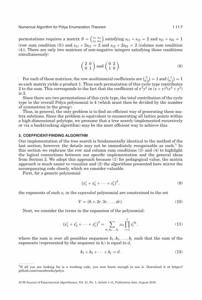
ALGORITHM 2: Coefficient CalculatorFunction sum sequences(Sl)

Finds τl (17) for Sl = {Slα}mα=1 (16)

Sl: a set of lists (of exponent sequences {kiα}ξ

i=1) for each polynomial Mrαα in Pπ (14).

. . . . . . . . . . . . . . . . . . . . . . . . . . . . . . . . . . . . . . . . . . . . . . . . . . . . . . . . . . . . . . . . . . . . . . . . . . . . . . . . . . . . . . . . . . . . . .Kl ← Sl1 × Sl2 × · · · × Slm = 〈{(kiα)ξi=1}m

α=1〉lcoeff ← 0for each {(kiα)ξi=1}m

α=1 ∈ Kl doif

∑mα=1 kiα = Ti ∀ i ∈ {1 . . . ξ} then

coeff ← coeff + ∏mα=1

( dα

{kiα }ξi=1

)end

end

return coeffFunction coefficient(T, Pπ , V)

Constructs S = {Sl} and calculates tπ (17)T: {Ti}ξ

i=1 target stoichiometry.Pπ : Polya polynomial representation for a single operation π in the group G (14).V: {Vα}m

α=1 possible exponents for each Mrαα (10).

. . . . . . . . . . . . . . . . . . . . . . . . . . . . . . . . . . . . . . . . . . . . . . . . . . . . . . . . . . . . . . . . . . . . . . . . . . . . . . . . . . . . . . . . . . . . . .if m = 1 then

if r1 > Ti ∀ i = 1..ξ thenreturn 0

elsereturn

( d1T1T2 ...Tξ

)end

elseT ← sorted(T)possible ← V1 × V2 × · · · × Vmcoeffs ← 0

for {k1α}mα=1 ∈ possible do

if∑m

α=1 k1α = T1 thenSl ← build Sl({k1α}m

α=1, V, Pπ , T)coeffs ← coeffs+ sum sequences(Sl)

endend

return coeffsend

confirm5 that the number of matrices scales exponentially with the number of colors(fixed group and number of elements in the set), linearly with the number of elementsin the set (fixed number of colors and group), and is linear with the group size (fixednumber of colors and elements in the set). The number of entries in the matrix S istξ (see the discussion above Equation (3)) and the height of the entries is (roughly)bounded by the number of cycles and (very roughly) by the color frequencies dividedby cycle lengths. This makes computing a time estimate based on these factors verydifficult, but in the worst case, it could grow like the tξ -th power of the average size of theentries, which will depend on the size of the target frequencies, and so on. This wouldbe a very complex function to estimate, but we may expect it to grow exponentially for

5Figures are included in the code repository. See supplementary material.



Fig. 4. Normalized algorithm scaling with the number of relevant matrices to enumerate. For large matrixcounts, the behavior appears linear, supporting the hypothesis that the algorithm scales roughly with thenumber of matrices. The scatter is appreciable only for small matrix counts (less than 106).

Fig. 5. Log plot of the algorithm scaling as the number of colors increases. Since the number of variablesxi in each polynomial increases with the number of colors, the combinatoric complexity of the expandedpolynomial increases drastically with each additional color; this leads to an exponential scaling. The linearfit to the logarithmic data has a slope of 0.403.

very large input. We did not find that to be an impediment for the sizes of problems weneeded to solve.

4.2. Experiments Demonstrating Algorithm Scaling

In Figure 5, we plot the algorithm’s scaling as the number of colors in the enumer-ation increases (for a fixed group and number of elements). For each r-cycle in thedisjoint-cyclic form of a group operation, we construct a polynomial with ξ variables,where ξ is the number of colors used in the enumeration. Because the group opera-tion results in a product of these polynomials, increasing the number of colors by 1increases the combinatoric complexity of the polynomial expansion exponentially. For



Fig. 6. Algorithm scaling as the number of elements in the finite set increases (for two colors). The Polyapolynomial arises from the group operations’ disjoint-cyclic form, so more elements in the set results in aricher spectrum of possible polynomials multiplied together. Because of the algorithms aggressive pruningof terms, the exact disjoint-cyclic form of individual group operations has a large bearing on the algorithm’sscaling. As such, it is not surprising that there is some scatter in the timings as the number of elements inthe set increases.

this scaling experiment, we used the same transitive group acting on a finite set with20 elements for each data point but increased the number of colors in the fixed colorterm T . We chose T by dividing the number of elements in the group as equally aspossible; thus for two colors, we used [10, 10]; for three colors we used [8, 6, 6], then[5, 5, 5, 5], [4, 4, 4, 4, 4], and so on. Figure 5 plots the log10 of the execution time (inms) as the number of colors increases. As expected, the scaling is linear (on the logplot).

As the number of elements in the finite set increases, the possible Polya polynomialrepresentations for each group operation’s disjoint-cyclic form increases exponentially.In the worst case, a group acting on a set with k elements may have an operation withk 1-cycles; on the other hand, that same group may have an operation with a singlek-cycle, with lots of possibilities in between. Because of the richness of possibilities, itis almost impossible to make general statements about the algorithm’s scaling withoutknowing the structure of the group and its classes. In Figure 6, we plot the scaling fora set of related groups (all are isomorphic to the direct product of S3 × S4) applied tofinite sets of varying sizes. Every data point was generated using a transitive groupwith 144 elements. Thus, this plot shows the algorithm’s scaling when the group isthe same and the number of elements in the finite set changes. Although the scalingappears almost linear, there is a lot of scatter in the data. Given the rich spectrum ofpossible Polya polynomials that we can form as the set size increases, the scatter is notsurprising.

Finally, we consider the scaling as the group size increases (Figure 7). For this test, weselected the set of unique groups arising from the enumeration of all derivative superstructures of a simple cubic lattice for a given number of sites in the unit cell [Hartand Forcade 2008]. Since the groups are formed from the symmetries of real crystals,they arise from the semidirect product of operations related to physical rotations andtranslations of the crystal. In this respect, they have similar structure for comparison.In most cases, the scaling is obviously linear; however, the slope of each trend variesfrom group to group. This once again highlights the scaling’s heavy dependence on



Fig. 7. Normalized algorithm scaling with group size for an enumeration problem from solid state physics[Hart and Forcade 2008]. We used the unique permutation groups arising from all derivative super structuresof a simple cubic lattice for a given number of sites in the unit cell. The behavior is generally linear withincreasing group size.

the specific disjoint-cyclic forms of the group operations. Even for groups with obvioussimilarity, the scaling may differ.

4.3. Comparison with Computer Algebra Systems

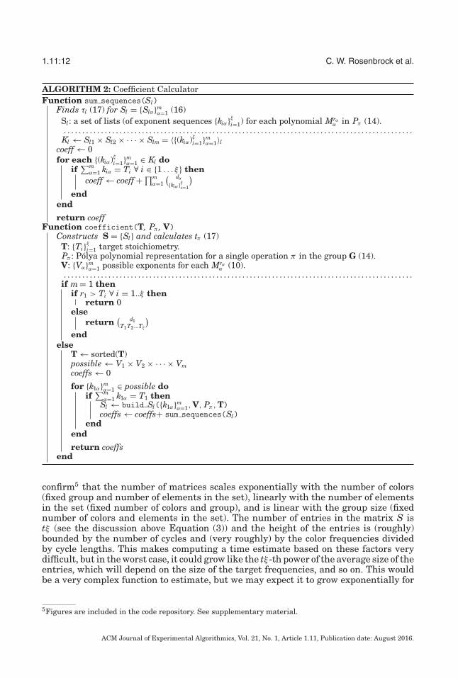
In addition to the explicit timing analysis and experiments presented above, we alsoran a group of representative problems with our algorithm and MATHEMATICA (a commonCAS). We also attempted the tests with MAPLE but were unable to obtain consistentresults between multiple runs of the same problems.6 So, we have opted to exclude theMAPLE timing results. For the comparison with MATHEMATICA, we used MATHEMATICA’sExpand and Coefficient functions to return the relevant coefficient from the Polyapolynomial (see Figure 8).

5. SUMMARY

Until now, no low-level, numerical implementation of Polya’s enumeration theorem hasbeen readily available; instead, a CAS was used to symbolically solve the polynomialexpansion problem posed by Polya. While CAS’s are effective for smaller, simpler cal-culations, as the difficulty of the problem increases, they become impractical solutions.Additionally, codes that perform the actual enumeration of the colorings are often im-plemented in low-level codes, and interoperability with a CAS is not necessarily easyto automate.

We presented a low-level, purely numerical algorithm and code that exploits theproperties of polynomials to restrict the combinatoric complexity of the expansion.By considering only those coefficients in the unexpanded polynomials that might con-tribute to the final answer, the algorithm reduces the number of terms that must beincluded to find the significant term in the expansion.

6The inconsistency manifests in MAPLE sometimes returning 0 instead of the correct result and sometimesrunning the same problem unpredictably in hours or seconds.



Fig. 8. Comparison of the CPU time (a) and memory usage (b) between the FORTRAN implementation of ouralgorithm and MATHEMATICA as the number of colors increases. These are the times needed to generate thedata in Figure 5.

Because of the algorithm scaling’s reliance on the exact structure of the group andthe disjoint-cyclic form of its operations, a rigorous analysis of the scaling is not possiblewithout knowledge of the group. Instead, we presented some numerical timing resultsfrom representative, real-life problems that show the general scaling behavior.

In contrast to the CAS solutions whose execution times range from milliseconds tohours, our algorithm consistently performs in the millisecond to second regime, evenfor complex problems. Additionally, it is already implemented in both high- and low-level languages, making it useful for confirming enumeration results. This makes it aneffective substitute for alternative CAS implementations.

REFERENCES

Stefano Curtarolo, Gus L. W. Hart, Marco Buongiorno Nardelli, Natalio Mingo, Stefano Sanvito, and OhadLevy. 2013. The high-throughput highway to computational materials design. Nat. Mater. 12, 3 (MAR2013), 191–201. DOI:http://dx.doi.org/10.1038/NMAT3568

Kecai Deng and Jianguo Qian. 2014. Enumerating stereo-isomers of tree-like polyinositols. J. Math. Chem.52, 6 (2014), 1581–1598.

Roberto Dovesi, Roberto Orlando, Alessandro Erba, Claudio M. Zicovich-Wilson, Bartolomeo Civalleri,Silvia Casassa, Lorenzo Maschio, Matteo Ferrabone, Marco De La Pierre, Philippe D’Arco, Yves Nol,Mauro Caus, Michel Rrat, and Bernard Kirtman. 2014. CRYSTAL14: A program for the ab initio in-vestigation of crystalline solids. Int. J. Quant. Chem. 114, 19 (2014), 1287–1317. DOI:http://dx.doi.org/10.1002/qua.24658

Antoine Genitrini, Bernhard Gittenberger, Veronika Kraus, and Cecile Mailler. 2015. Associative and com-mutative tree representations for Boolean functions. Theor. Comput. Sci. 570 (2015), 70–101.

Modjtaba Ghorbani and Mahin Songhori. 2014. The enumeration of Chiral isomers of tetraammine plat-inum (II). Match-Communications in Mathematical and in Computer Chemistry 71, 2 (2014), 333–340.

Frank Harary. 1955. The number of linear, directed, rooted, and connected graphs. Trans. Am. Math. Soc.78, 2 (1955), 445–463.

Gus L. W. Hart and Rodney W. Forcade. 2008. Algorithm for generating derivative structures. Phys. Rev. B77 (Jun 2008), 224115. Issue 22. DOI:http://dx.doi.org/10.1103/PhysRevB.77.224115

Gus L. W. Hart and Rodney W. Forcade. 2009. Generating derivative structures from multilattices: Applica-tion to HCP alloys. Phys. Rev. B 80 (July 2009), 014120.

Gus L. W. Hart, Lance J. Nelson, and Rodney W. Forcade. 2012. Generating derivative struc-tures for a fixed concentration. Comp. Mat. Sci. 59 (2012), 101–107. DOI:http://dx.doi.org/10.1016/j.commatsci.2012.02.015

B. A. Kennedy, D. A. McQuarrie, and C. H. Brubaker Jr. 1964. Group theory and isomerism. Inorg. Chem. 3,2 (1964), 265–268.


http://dx.doi.org/10.1038/NMAT3568

http://dx.doi.org/10.1002/qua.24658

http://dx.doi.org/10.1002/qua.24658

http://dx.doi.org/10.1103/PhysRevB.77.224115

http://dx.doi.org/10.1016/j.commatsci.2012.02.015

http://dx.doi.org/10.1016/j.commatsci.2012.02.015


Peter Lackner, Harald Fripertinger, and Gerhard Nierhaus. 2015. Peter Lackner/tropical investigations. InPatterns of Intuition. Springer, Berlin, 279–313.

Yannis Manolopoulos. 2002. Binomial coefficient computation: Recursion or iteration? ACM SIGCSE BulletinInRoads 34 (Dec 2002). Issue 4. DOI:http://dx.doi.org/10.1145/820127.820168

James McGrane, Sanjaye Ramgoolam, and Brian Wecht. 2015. Chiral ring generating functions & branchesof moduli space. arXiv preprint arXiv:1507.08488 (2015).

Sami Mustapha, Philippe DArco, Marco De La Pierre, Yves Nol, Matteo Ferrabone, and Roberto Dovesi.2013. On the use of symmetry in configurational analysis for the simulation of disordered solids. J.Phys.: Condens. Matter 25, 10 (2013), 105401. http://stacks.iop.org/0953-8984/25/i=10/a=105401.

George Polya. 1937. Kombinatorische anzahlbestimmungen fr gruppen, graphen und chemische verbindun-gen. Acta Math. 68, 1 (1937), 145–254.

George Polya and Ronald C. Read. 1987. Combinatorial Enumeration of Groups, Graphs, and ChemicalCompounds (1987).

Jianguo Qian. 2014. Enumeration of unlabeled uniform hypergraphs. Discr. Math. 326, 1 (2014), 66–74.R. W. Robinson, F. Harry, and A. T. Balaban. 1976. The numbers of chiral and achiral alkanes and monosub-

stituted alkanes. Tetrahedron 32, 3 (1976), 355–361.Masahiko Taniguchi, Sarah Henry, Richard J. Cogdell, and Jonathan S. Lindsey. 2014. Statistical consider-

ations on the formation of circular photosynthetic light-harvesting complexes from rhodopseudomonaspalustris. Photosynth. Res. 121, 1 (2014), 49–60.

J. Tura, R. Augusiak, A. B. Sainz, B. Lucke, C. Klempt, M. Lewenstein, and A. Acın. 2015. Nonlocalityin many-body quantum systems detected with two-body correlators. arXiv preprint arXiv:1505.06740(2015).

Received December 2015; revised May 2016; accepted June 2016


http://dx.doi.org/10.1145/820127.820168

http://stacks.iop.org/0953-8984/25/i$=$10/a$=$105401

numerical algorithm for polya enumeration theorem´numerical algorithm for polya enumeration...

Documents