numerical modeling of flow control in a boundary-layer- ingesting offset inlet ... ·...

American Institute of Aeronautics and Astronautics

1

Numerical Modeling of Flow Control in a Boundary-Layer-Ingesting Offset Inlet Diffuser at Transonic Mach Numbers

Brian G. Allan* and Lewis R. Owens† NASA Langley Research Center, Hampton, VA, 23681

Abstract

This paper will investigate the validation of the NASA developed, Reynolds-averaged Navier-Stokes (RANS) flow solver, OVERFLOW, for a boundary-layer-ingesting (BLI) offset (S-shaped) inlet in transonic flow with passive and active flow control devices as well as a baseline case. Numerical simulations are compared to wind tunnel results of a BLI inlet experiment conducted at the NASA Langley 0.3-Meter Transonic Cryogenic Tunnel. Comparisons of inlet flow distortion, pressure recovery, and inlet wall pressures are performed. The numerical simulations are compared to the BLI inlet data at a free-stream Mach number of 0.85 and a Reynolds number of approximately 2 million based on the fan-face diameter. The numerical simulations with and without tunnel walls are performed, quantifying tunnel wall effects on the BLI inlet flow. A comparison is made between the numerical simulations and the BLI inlet experiment for the baseline and VG vane cases at various inlet mass flow rates. A comparison is also made to a BLI inlet jet configuration for varying actuator mass flow rates at a fixed inlet mass flow rate. Overall, the numerical simulations were able to predict the baseline circumferential flow distortion, DPCPavg, very well within the designed operating range of the BLI inlet. A comparison of the average total pressure recovery showed that the simulations were able to predict the trends but had a negative 0.01 offset when compared to the experimental levels. Numerical simulations of the baseline inlet flow also showed good agreement with the experimental inlet centerline surface pressures. The vane case showed that the CFD predicted the correct trends in the circumferential distortion levels for varying inlet mass flow but had a distortion level that was nearly twice as large as the experiment. Comparison to circumferential distortion measurements for a 15° clocked 40 probe rake indicated that the circumferential distortion levels are very sensitive to the symmetry of the flow and that a misalignment of the vanes in the experiment could have resulted in this difference. The numerical simulations of the BLI inlet with jets showed good agreement with the circumferential inlet distortion levels for a range of jet actuator mass flow ratios at a fixed inlet mass flow rate. The CFD simulations for the jet case also predicted an average total pressure recovery offset that was 0.01 lower than the experiment as was seen in the baseline. Comparisons of the flow features for the jet cases revealed that the CFD predicted a much larger vortex at the engine fan-face when compare to the experiment.

Nomenclature AC = inlet capture (highlight) area; area enclosed by inlet highlight and tunnel wall, in.2 A0 = inlet mass-flow stream-tube area at free-stream conditions, in.2 A0/AC = inlet mass-flow ratio c = chord length of the vortex generator vane, in. CP = coefficient of pressure, =(P-P∞)/(1/2 ρ∞V2) D = duct diameter at AIP * Research Scientist, Flow Physics and Control Branch, MS 170, NASA Langley Research Center, Hampton, VA 23681, AIAA Senior Member. † Research Engineer, Flow Physics and Control Branch, MS 170, NASA Langley Research Center, Hampton, VA 23681, AIAA Senior Member.

https://ntrs.nasa.gov/search.jsp?R=20080013580 2018-07-07T15:57:50+00:00Z


2

DPCPavg = average SAE circumferential distortion descriptor DPRPi = SAE radial distortion descriptor for ring i on AIP total-pressure rake h = height of vortex generator vane, in. i = ring number on AIP total-pressure rake (i=1 at hub and 5 at the tip) M = Mach number PT = total pressure, psi PTavg = area weighted average total pressure at AIP PTavg/PT0 = inlet recovery pressure ratio ReD = Reynolds number based on duct AIP diameter D TT = total temperature, °R ρ = density, lbm/ft3 Subscripts: ∞ = free-stream conditions Abbreviations: ACTMFR actuator mass flow ratio, =(jet mass flow rate)/(inlet mass flow rate) AFC active flow control AIP aerodynamic interface plane BLI boundary-layer ingesting BWB blended-wing-body CFD computational fluid dynamics DOE design of experiment NASA National Aeronautics and Space Administration SAE Society of Automotive Engineers UEET Ultra Efficient Engine Technology VG vortex generator

I. Introduction N an effort to reduce the environmental impact of commercial aircraft using revolutionary propulsion technologies, NASA initiated the Ultra Efficient Engine Technology (UEET) program1. One of the elements of

the UEET program is the application of flush-mounted, boundary layer ingesting (BLI), offset inlets on the aft portion of an aircraft. System studies for the Blended Wing Body (BWB) transport have shown significant reductions in fuel burn by using this type of inlet2. For the BWB vehicle, a BLI inlet placed on the upper rear surface of the wing would have a boundary layer to inlet height ratio of 30%. The ingestion of such a large boundary layer coupled with the S-shaped offset of the inlet diffuser, results in a large flow distortion at the engine fan face3-5. Experiments and numerical simulations have shown that inlet distortion can be improved for the ingestion of a 30% thick boundary layer, to acceptable operational levels, using flow control devices located inside the inlet4,6.

The application of flow control devices for inlets has been investigated since the late 1940s when Taylor7 used vortex generator (VG) vanes to re-energize the boundary layer to prevent flow separation. Inlet flow control research continued into the 1950s by Grose and Taylor8, Valentine and Carrol9,10, and Pearcy and Stuart11. The early design strategies used here were based on preventing flow separation within the inlet duct and were based on two-dimensional boundary layer concepts. As a result of this design approach, the VG vanes did not perform well for inlets with regions of large secondary flows.

In 1973, Kaldschmidt, Syltebo, and Ting12 demonstrated that one could restructure the development of the secondary flow improving engine fan-face distortion levels. This work marked a shift in inlet flow control design moving away from separation control to a global manipulation of the secondary inlet flow. This new design approach would require inlet flow control designs to solve the three-dimensional viscous flow equations. The paper by Anderson and Levy13 demonstrated how passive flow control devices could be designed by solving the three-dimensional reduced Navier-Stokes equations. Today inlet flow control designs are using Design of Experiments (DOE) to build a response surface model using several design factors and optimizing the flow control design to

I


3

minimize flow distortion and high cycle fatigue while maximizing pressure recovery, all over a desired range of operating flow conditions for compact S-shaped inlet diffusers14-24.

While there has been significant research on inlet flow control, there has been very little research on flow control for inlets with large BLI. The first experiments, using passive flow control for a BLI inlet were, performed by Anabtawi, Blackwelder, Liebeck, and Lissaman5 for an offset or S-shaped duct at very low Mach numbers. This experiment was able to demonstrate that passive vane devices could be used to improve the engine fan-face distortion to operation levels. Expanding on this research Gorton, Owens, Jenkins, Allan, and Schuster4 performed low Mach experiments on a S-shaped BLI inlet using active flow control jets and passive VG vanes. This experiment showed that jets could be used to reduce the flow distortion. It also provided experimental data for the validation of OVERFLOW, a NASA developed Reynolds-averaged Navier-Stokes (RANS) flow solver6. Experimental data for the baseline BLI inlet in transonic flow was performed by Berrier and Morehouse25, which were also used to validate OVERFLOW6. These validations of the flow solver provided confidence in the design of flow control jets for a flow control BLI inlet experiment at transonic Mach numbers26. The flow solver was used to identify candidate jet actuator locations, which were then used in the modification of the baseline BLI inlet model. A DOE was also performed for a VG vane configuration to be tested at transonic Mach numbers performed by Allan, Owens, and Lin27.

This research will use the experimental wind tunnel results of Owens, Allan, and Gorton26 for the validation of OVERFLOW. A comparison of the engine fan-face distortion levels, average total pressure recovery, and static inlet wall pressures are made for a single jet actuator and vane configuration. Comparison between experiment and the numerical simulations will be made looking at variations in actuator mass flow rates at a fixed inlet condition. For the VG vane case, an inlet mass flow sweep will be compared to the numerical simulations. The numerical simulations will also be performed with and without wind tunnel walls in order to quantify the wall effects.

II. Numerical Modeling Approach The steady-state flow field for the BLI offset inlet with VG vanes and jets was computed using the flow solver

code, OVERFLOW28,29, developed at NASA. This code solves the compressible RANS equations using the diagonal scheme of Pulliam and Chaussee30. The RANS equations are solved on structured grids using the overset grid framework of Steger, Dougherty, and Benek31. This overset grid framework allows for the use of structured grids for problems that have complex geometries. To improve the convergence of the steady-state solution, the OVERFLOW code also includes a low-Mach number preconditioning option and a multigrid acceleration routine. All of the simulations in this study used Menter's two-equations (k-ω) Shear-Stress Transport (SST) turbulence model32. The SST turbulence model was found to be the best turbulence model option in OVERFLOW for the simulation of streamwise vortices embedded in a boundary layer33.

The numerical simulations were performed using the parallel version of the OVERFLOW code developed by Buning34. This code uses the Message-Passing Interface (MPI) and can run on a tightly-coupled parallel machine or a network of workstations. The code distributes zones to individual processors and can split larger individual zones across multiple processors using a domain decomposition approach.

The structured overset grid system was generated using the Chimera Grid Tools package35. Figure 1 shows a close-up view of the overset grids near the VG vanes on the inlet surface. The vanes were modeled as rectangular fins, which were shown to be comparable to fully modeled vanes33. Figure 2 shows a close-up view of the nozzle grid system for the jet simulation. The steady jet is skewed 90o to the frees-stream flow and pitched at an inclined angle of 30o to the surface. These pitch and skew angles for the jet result in the generation of a single streamwise vortex while imparting a side momentum force to the oncoming flow. The jets were simulated by modeling the nozzle geometry twelve diameters below the inlet surface. This simplified the boundary condition by allowing the flow inside the nozzle to develop and adjust to the flow at the jet exit. Figure 3 shows the inlet grids with the jet grids on the bottom surface of the inlet. Figure 4 shows the overset grid along the centerline of the inlet.

III. Wind Tunnel Experiment 1. Experimental Wind Tunnel Setup The numerical simulations of the BLI inlet with flow control jets and vanes are compared to the experimental

wind tunnel results of Owens, Allan, and Gorton26. The transonic BLI inlet experiments were conducted at NASA Langley’s 0.3-Meter Transonic Cryogenic Tunnel (0.3-Meter Tunnel) for a BLI offset inlet mounted on the tunnel sidewall. The experimental data was taken over a Mach number range of 0.78 to 0.88 with a Reynolds number range of ReD = 2·106 to 4·106, where the engine fan-face or Aerodynamic Interface Plane (AIP) diameter, D was equal to 2.448 inches. This experiment was able to test the BLI inlet at actual flight Mach numbers expected for the


4

BWB aircraft. A previous experiment by Berrier and Morehouse25 evaluated the baseline inlet at flight Mach and Reynolds number where ReD ranged from 5.1·106 to 13.9·106. The experiment of Berrier and Morehouse25 showed that the Reynolds number had a small effect on the circumferential distortion and average total pressure recovery levels.

This experiment generated a boundary layer that was approximately 35% of the inlet height ratio. This boundary layer was measured at the same streamwise tunnel station as inlet highlight and was placed between the outer inlet cowling and wind tunnel wall. The inlet had 176 possible jet locations distributed along 11 different streamwise stations inside of the inlet. Subsets of these jets were connected to 16 individual solenoid actuators. The jet configuration used in this investigation had four jets connected to each solenoid actuator resulting in a total of 64 jets. Using the solenoid actuators, the jets could be turned on and off in groups of four to determine which jet locations of the subset of 64 jets performed best. The numerical simulations were compared to experimental data taken using a group of 36 out of the 64, which were found to have good performance.

2. Inlet Mass Flow Area Ratio The inlet mass flow rate was nondimensionalized by the area ratio A0/AC where A0 is defined as the area in the

free-stream flow such that: ρ0U0A0 = ρCUCAC (1)

where ρCUCAC is the inlet mass flow rate. The inlet capture area, AC, is defined at the area that encloses the cowling highlight with the bottom wall. The equation above shows that the mass flow rate through the area A0, defined as being located in a uniform free-stream flow, is equal the inlet mass flow rate. Therefore, when A0/AC is unity the stream-tube going into the inlet is ideally not expanding or shrinking for the inlet in a free-stream flow. The inlet in this study was mounted on the tunnel wall ingesting a boundary layer; therefore an area ratio of unity does not exactly result in a straight stream-tube. However this area ratio does provide a good physical insight to the character of the flow approaching the inlet as well as a nondimensional inlet mass flow rate parameter. Similarly, an A0/AC less than one would ideally indicate that the stream-tube approaching the inlet is expanding and for A0/AC greater than one it would be shrinking.

3. Distortion Descriptor The inlet distortion in this investigation was described by the SAE circumferential distortion descriptor,

DPCPavg, which is defined in the Aerospace Recommended Practice (ARP) 1420 standard36. The DPCPavg is equal to the average distortion intensity defined in (2).

DPCPavg = 1/Nrings ∑(i=1-5) Intensityi (2)

where i is the ring number on the AIP rake and Nrings is the total number of rings. The Intensity for each ring is defined as,

Intensityi = (PAVi - PAVLOWi)/PAVi (3)

where PAVi is the average total pressure of ring i and PAVLOWi, the area average of the low total pressure region below PAVi.

4. VG Vane Experiment The VG vane configuration used for this experiment was designed by performing a DOE optimization

minimizing the circumferential flow distortion and first five harmonic amplitudes while maximizing the total pressure recovery. The design was specified to have a single row of vanes with 12 vanes on the sides and 12 vanes on the bottom of the inlet. The optimization was also at a fixed A0/AC of 0.59 for a free-stream Mach number of 0.784 and was not optimized over a range of inlet mass flow ratios. The design was performed at a fixed inlet mass flow rate since the computational cost of performing the design over a wide range of inlet mass flow would have been prohibitively expensive using the fully gridded approach for the VG vanes taken here. The design was also constrained to a single row of vanes in order to simplify the vane installation inside of the inlet. This constraint to a single row resulted in vanes that were relatively large compared to the inlet diameter. However the vanes are approximately 30% of the ingested boundary layer height, which is relatively small when compared to the boundary layer. More details of the vane optimization are described by Allan, Owens, and Lin27. Figure 5 shows the vane configuration used in the experiment where the vanes are located a distance x/D=0.5 downstream of the inlet lip highlight. The side vanes had a height of h/D = 0.065 and the bottom vanes had a height of h/D =0.074 where both


5

sets of vanes had chord lengths of c/D=0.15. The side vanes were positioned at an angle of 11.5 degrees to the free-stream direction and the bottom vanes at 12.9 degrees.

5. Jet Actuator Experiment The wind tunnel experiment by Owens, Allan, and Gorton26 evaluated many different jet patterns. A single jet

pattern was used in this investigation. The jet configuration is shown in Fig. 6 where there are a total of 36 jets each with an orifice diameter of 0.040 inches or a nondimensional diameter of djet/D = 0.0163. The jets were angled 90° to the flow and inclined 30° from the surface. All of the jets were blowing from the bottom centerline outwards toward top of the inlet, opposing the natural secondary flow of the S-shaped inlet. All but two of the jets were on the bottom of the inlet near the entrance. This jet pattern was used in this investigation since it performed well and had the most experimental data. The experimental data for this case also included an evaluation of the control jets over a range of ReD from 1.8·106 to 3.8·106.

6. Inlet Mass flow Rate The inlet was designed to operate over an A0/AC range from 0.46 to 0.65 at a cruise Mach number of 0.85. The

wind tunnel experiment was only able to achieve a maximum A0/AC of 0.54 for a free-stream Mach of 0.85. It’s believed that the inlet was either limited by the chocking of the flow at the AIP rake or at an exit vent valve downstream of the inlet rake. While values of A0/AC below 0.46 are not within the design or operational limits of the inlet, it was of interest to analyze the performance trends of the inlet and to compare them with the numerical simulations.

7. Wall Correction for Inlet Centerline Surface Pressures The wind tunnel sidewalls for the experiment were adapted in order to maintain a constant 0.85 Mach number

ahead of the inlet. They were also expanded near the inlet in an effort to reduce the tunnel blockage from the inlet. As a result, the static pressure in the wind tunnel had a slight variation in the streamwise directions. This variation produced an offset in the static wall pressure inside the inlet when comparing the CFD results to the experimental data. In an attempt to correct for this wall effect, a simple wall correction was made. This correction was made by subtracting a wall pressure measurement on the opposite wall of the inlet near the same streamwise station as the inlet highlight. While this is a somewhat simplified wall correction approach, it seemed to work well for inlet flows, which do not have flow separation at the entrance of the inlet.

IV. Results Numerical simulations for the baseline inlet and the inlet with vanes and jets are compared to experimental wind

tunnel results. The baseline and vane cases were compared to experimental results at a single free-stream Mach and Reynolds number for varying inlet mass flow ratios. The inlet simulations with jets were performed at a fixed free-stream Mach and Reynolds number at a single inlet mass flow rate for varying jet actuator mass flow rates. All of the BLI inlet simulations were performed with the inlet mounted on a flat plate where the length ahead of the plate was adjusted in order to match the experimental boundary layer height at the inlet. The inlet was also simulated with the tunnel walls for some cases in order to quantify the tunnel wall effects on the inlet simulations.

A. Baseline BLI Inlet Numerical simulations for the baseline inlet were made for a free-stream Mach number of 0.85 and a Reynolds

number of ReD = 2.2⋅106 with a boundary layer height of δ/D = 0.245 (0.6 inches) at the boundary layer rake location to the side of the inlet cowling. These numerical simulation are compared to the experimental data where the Mach number was held at a constant 0.85 upstream of the inlet with a Reynolds number of ReD=3.8⋅106. A previous baseline numerical comparison was made by Allan and Berrier3 for the BLI inlet at a flight Reynolds number of a ReD=13.8⋅106 showing good agreement with the experiment. The current wind tunnel test was performed using warm Nitrogen gas (300° K) resulting in a lower Reynolds number than the previous baseline study. The previous wind tunnel test by Berrier and Morehouse25 showed the Reynolds number to have a small effect on the baseline flow over a ReD range of 5.1⋅106 to 13.9⋅106.

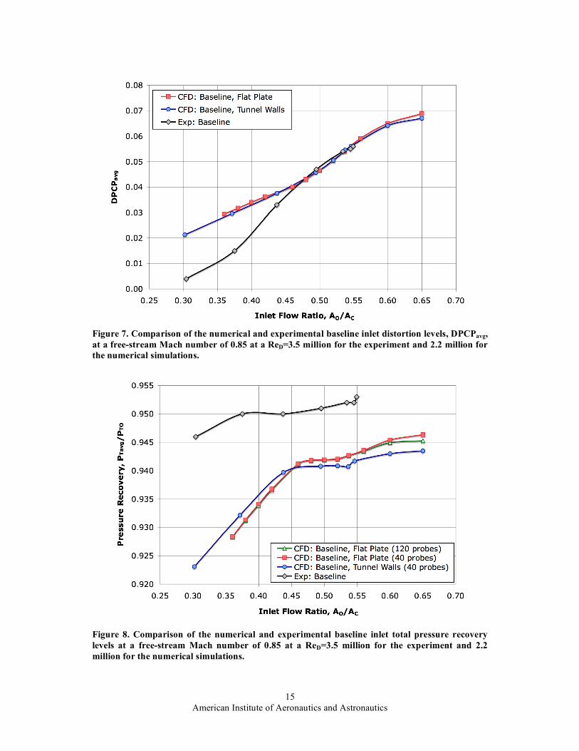
1. Inlet Distortion Figure 7 shows a comparison of the numerical and experimental baseline DPCPavg distortion levels for various

inlet mass flow ratios. The numerical simulations were performed over an A0/AC range of 0.30 to 0.65 and are compared to the experimental results over an A0/AC range from 0.30 to 0.55. All of the DPCPavg distortion levels and average total pressure recovery calculations for the numerical simulations were made by interpolating the CFD results onto the same 40-probe rake locations used in the experiment. This was done in order to match the measurement resolution of the experiment where the distortion levels for the numerical results were seen to be sensitive to 40 and 120 probe resolution measurements in some cases.


6

This baseline comparison shows that the numerical simulations predicted the DPCPavg distortion levels very well over an A0/AC range from 0.46 to 0.55. At an A0/AC of 0.44, which is just below the operational range of the inlet mass flow, the baseline inlet experimental results showed a DPCPavg distortion level of 0.033. The numerical simulations at the maximum inlet mass flow ratio for cruise (A0/AC=0.65) are predicting a DPCPavg of 0.069 where acceptable distortion levels are below 0.04. Figure 7 shows how the circumferential distortion levels for the baseline flow are above this 0.04 level for the operational range of A0/AC of 0.46 to 0.65. Therefore the baseline flow needs to be improved using flow control to reduce the distortion level below 0.04 in the designed operational inlet mass flow range.

While the inlet mass flow ratios below 0.46 are outside of the operation range of the inlet, numerical simulations were made to compare with the experimental baseline data. Figure 7 shows how the numerical results start to diverge from the experimental data below 0.46 where the CFD is predicting a higher inlet distortion than measured in the experiment. Below an A0/AC of 0.46, the numerical simulations are showing a large separated flow that’s forming at the entrance of the inlet. Figure 9 shows Mach contours at the centerline of the numerical simulations of the BLI inlet. This figure shows four inlet mass flow ratios ranging from A0/AC of 0.537 down to 0.38 for a fixed Mach number of 0.877. These contours show how the boundary layer being ingested into the inlet starts to thicken at the entrance of the inlet as the inlet mass flow ratio is decreased. At an A0/AC equal to 0.42, a small separation bubble starts to form, becoming larger when A0/AC is decreased to 0.38. Predicting the distortion values at these low inlet flows using CFD is very challenging because of the large flow separation ahead of the inlet. While it’s interesting to note the difference in the distortion levels at these low inlet mass flow ratios, it should be noted that these conditions are below the designed operating range of the inlet where being able to predict the onset of flow separation is more important than matching the actual distortion level.

Figure 7 also includes the distortion levels for the BLI inlet modeling the wind tunnel walls. This comparison shows that modeling the tunnel walls did not have a significant impact on the circumferential distortion levels for the baseline case.

2. Pressure Recovery Comparisons of the average total pressure recovery levels are presented in Fig. 8 where the numerical

simulations are showing an offset of 0.01 lower than the experimental levels for A0/AC above 0.45. The numerical simulations have a significant drop in the total pressure recovery below A0/AC of 0.45 due to the flow separation ahead of the inlet where the experimental data shows a similar drop starting near 0.37. This suggests that the CFD is predicting the flow separation at the entrance of the inlet starting at a much higher inlet mass flow ratio as compared to the experiment. The slope of the pressure recovery drop at the low inlet mass flow ratios is seen to be much steeper in the CFD simulations as compared to the experiment. Figure 8 also includes the total pressure recovery for the CFD simulations with the tunnel walls. As was seen in the distortion levels, adding the tunnel walls only had a small effect on the total pressure recovery for the baseline case. The reason for the offset in the total pressure recovery levels is not known. Possible sources could include differences between the experimental and numerical boundary layer profiles since the size of the boundary layer is the main source of the low total pressure recovery levels. Figure 8 also shows the effect of the 40-probe rake resolution by comparing it to a 120-robe rake interpolated CFD simulation data. This comparison between the different rake interpolations, for the same CFD simulations, shows little effect on the baseline total pressure recovery. There is a slight difference for the CFD simulation at the 0.65 inlet mass flow ratio case and is related to a slight change in the shape of the low-pressure region such that the 40-probe rake has a total pressure that is a little higher than the 120-probe rake.

3. AIP Total Pressure Ratio Contours Comparisons of the total pressure ratio contours, PT/PT0, at the AIP are shown in Fig. 10 for four inlet mass flow

ratio cases. These contour plots show the CFD and experimental results along with the CFD results interpolated onto the 40-probe rake that were used to compute the pressure recovery and DPCPavg distortion levels. The high inlet mass flow ratio case in Fig. 10(a) shows good agreement with the experimental results where the CFD results show a minimum total pressure ratio that is 0.01 lower than the experiment at the bottom of the AIP. This comparison also shows a low total pressure region that is slightly thicker than the one seen in the experimental measurements. The numerical simulation also predicted a pressure recovery that is 0.009 lower than the experimental measurement at this inlet mass flow rate. Figure 10(b) show a comparison of the total pressure ratio contour plots for A0/AC of 0.50, which compares well to the contours from the experiment. The CFD also matched the distortion and pressure recovery levels very well with only slight differences in the shape of the low total pressure region. Figures 10(c) and (d) show the contour plots for low inlet flow rates where the CFD predicts a lower minimum total pressure region at the bottom of the AIP as compared to the experiment. The differences in these contours is thought to be related to the prediction of the flow separation ahead of the inlet, which does not seem to be predicted well by the flow solver.


7

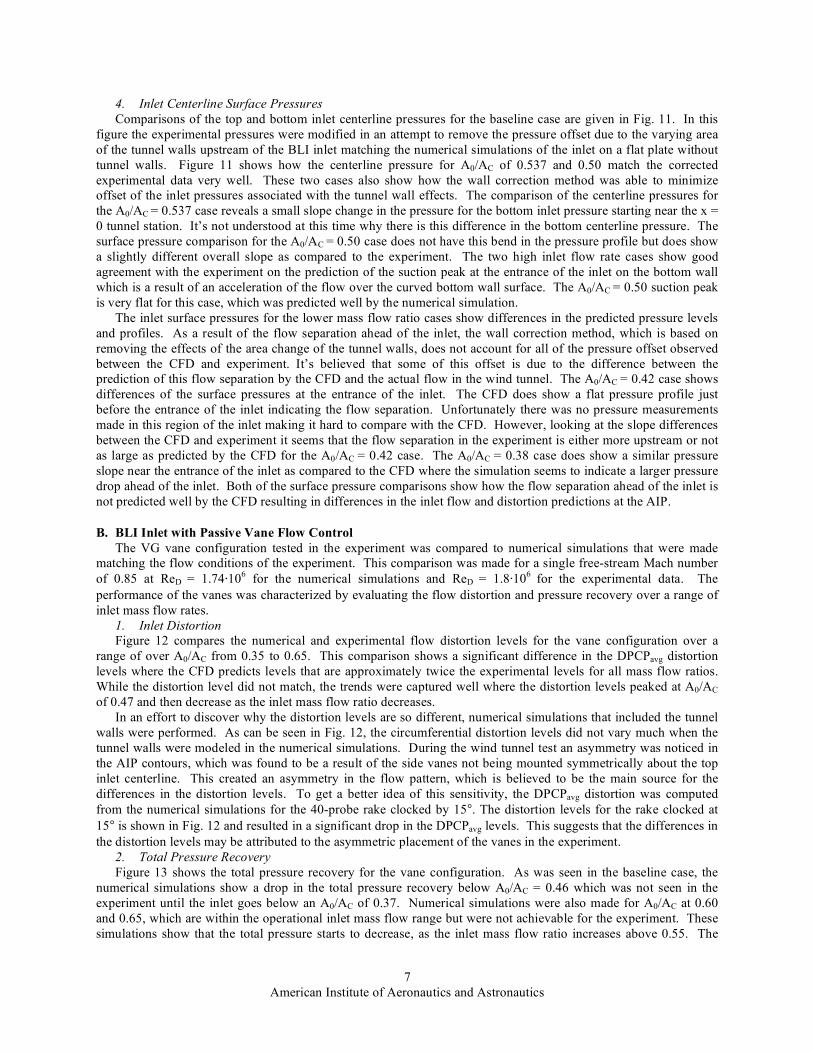
4. Inlet Centerline Surface Pressures Comparisons of the top and bottom inlet centerline pressures for the baseline case are given in Fig. 11. In this

figure the experimental pressures were modified in an attempt to remove the pressure offset due to the varying area of the tunnel walls upstream of the BLI inlet matching the numerical simulations of the inlet on a flat plate without tunnel walls. Figure 11 shows how the centerline pressure for A0/AC of 0.537 and 0.50 match the corrected experimental data very well. These two cases also show how the wall correction method was able to minimize offset of the inlet pressures associated with the tunnel wall effects. The comparison of the centerline pressures for the A0/AC = 0.537 case reveals a small slope change in the pressure for the bottom inlet pressure starting near the x = 0 tunnel station. It’s not understood at this time why there is this difference in the bottom centerline pressure. The surface pressure comparison for the A0/AC = 0.50 case does not have this bend in the pressure profile but does show a slightly different overall slope as compared to the experiment. The two high inlet flow rate cases show good agreement with the experiment on the prediction of the suction peak at the entrance of the inlet on the bottom wall which is a result of an acceleration of the flow over the curved bottom wall surface. The A0/AC = 0.50 suction peak is very flat for this case, which was predicted well by the numerical simulation.

The inlet surface pressures for the lower mass flow ratio cases show differences in the predicted pressure levels and profiles. As a result of the flow separation ahead of the inlet, the wall correction method, which is based on removing the effects of the area change of the tunnel walls, does not account for all of the pressure offset observed between the CFD and experiment. It’s believed that some of this offset is due to the difference between the prediction of this flow separation by the CFD and the actual flow in the wind tunnel. The A0/AC = 0.42 case shows differences of the surface pressures at the entrance of the inlet. The CFD does show a flat pressure profile just before the entrance of the inlet indicating the flow separation. Unfortunately there was no pressure measurements made in this region of the inlet making it hard to compare with the CFD. However, looking at the slope differences between the CFD and experiment it seems that the flow separation in the experiment is either more upstream or not as large as predicted by the CFD for the A0/AC = 0.42 case. The A0/AC = 0.38 case does show a similar pressure slope near the entrance of the inlet as compared to the CFD where the simulation seems to indicate a larger pressure drop ahead of the inlet. Both of the surface pressure comparisons show how the flow separation ahead of the inlet is not predicted well by the CFD resulting in differences in the inlet flow and distortion predictions at the AIP.

B. BLI Inlet with Passive Vane Flow Control The VG vane configuration tested in the experiment was compared to numerical simulations that were made

matching the flow conditions of the experiment. This comparison was made for a single free-stream Mach number of 0.85 at ReD = 1.74⋅106 for the numerical simulations and ReD = 1.8⋅106 for the experimental data. The performance of the vanes was characterized by evaluating the flow distortion and pressure recovery over a range of inlet mass flow rates.

1. Inlet Distortion Figure 12 compares the numerical and experimental flow distortion levels for the vane configuration over a

range of over A0/AC from 0.35 to 0.65. This comparison shows a significant difference in the DPCPavg distortion levels where the CFD predicts levels that are approximately twice the experimental levels for all mass flow ratios. While the distortion level did not match, the trends were captured well where the distortion levels peaked at A0/AC of 0.47 and then decrease as the inlet mass flow ratio decreases.

In an effort to discover why the distortion levels are so different, numerical simulations that included the tunnel walls were performed. As can be seen in Fig. 12, the circumferential distortion levels did not vary much when the tunnel walls were modeled in the numerical simulations. During the wind tunnel test an asymmetry was noticed in the AIP contours, which was found to be a result of the side vanes not being mounted symmetrically about the top inlet centerline. This created an asymmetry in the flow pattern, which is believed to be the main source for the differences in the distortion levels. To get a better idea of this sensitivity, the DPCPavg distortion was computed from the numerical simulations for the 40-probe rake clocked by 15°. The distortion levels for the rake clocked at 15° is shown in Fig. 12 and resulted in a significant drop in the DPCPavg levels. This suggests that the differences in the distortion levels may be attributed to the asymmetric placement of the vanes in the experiment.

2. Total Pressure Recovery Figure 13 shows the total pressure recovery for the vane configuration. As was seen in the baseline case, the

numerical simulations show a drop in the total pressure recovery below A0/AC = 0.46 which was not seen in the experiment until the inlet goes below an A0/AC of 0.37. Numerical simulations were also made for A0/AC at 0.60 and 0.65, which are within the operational inlet mass flow range but were not achievable for the experiment. These simulations show that the total pressure starts to decrease, as the inlet mass flow ratio increases above 0.55. The


8

numerical simulation for A0/AC of 0.65 shows a 0.05 decrease in the total pressure recovery, which is a fairly significant drop for an increase in the inlet mass flow rate.

A comparison of rake resolution on the total pressure recovery was made using the CFD simulation results. This comparison shows that a 120-probe rake predicts a total pressure recovery that is 0.005 lower than the 40-probe rake. This difference can be attributed to the low total pressure region at the top of the AIP that is not captured by the 40-probe rake. It’s not known if this low-pressure region at the top of the AIP exists in the wind tunnel experiment since it was limited to the 40-probe rake resolution.

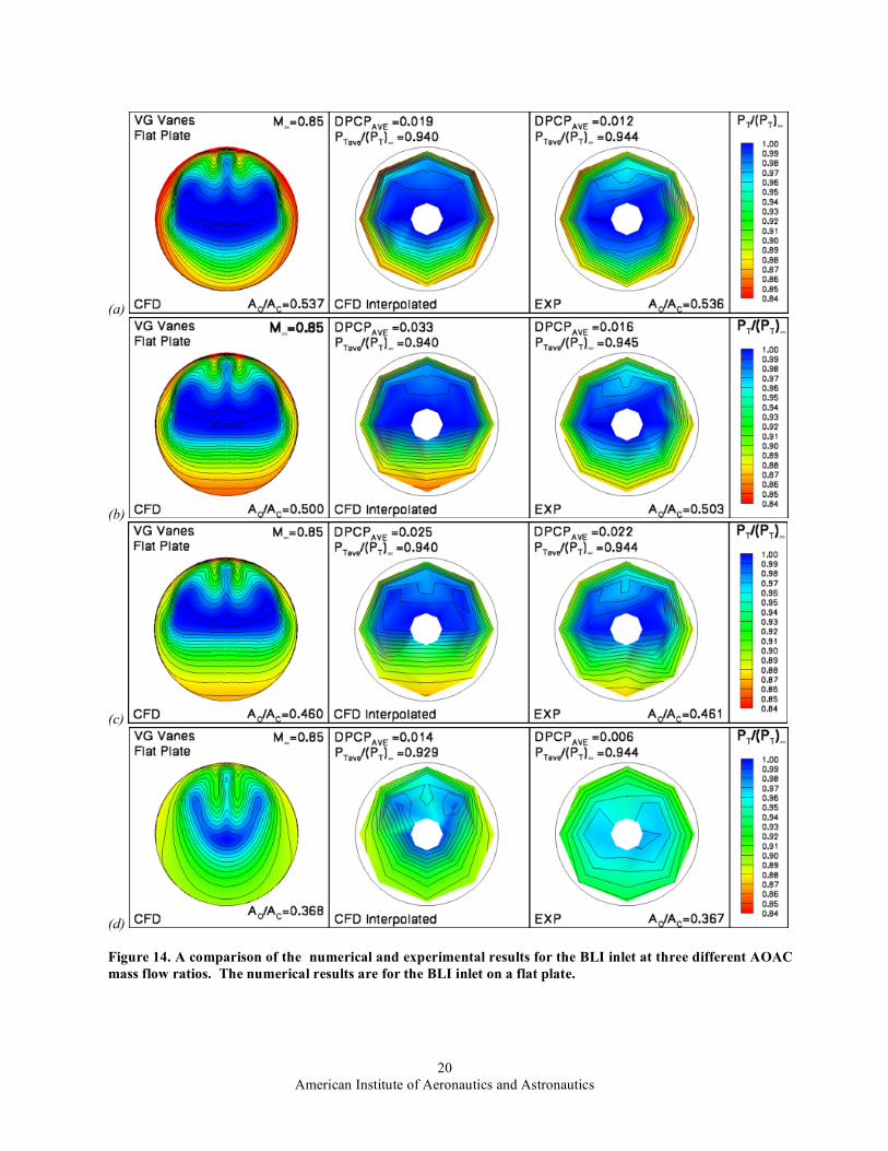
3. AIP Total Pressure Ratio Contours Figure 14 compares the total pressure ratio contours at the inlet AIP location for the numerical and experimental

vane results. The total pressure ratio contours in Fig. 14(a) show the comparison for an A0/AC of 0.537 where the numerical results compare well with the experiment. The experiment does show a thinner low total pressure region on the bottom of the inlet AIP as compared to the CFD contours. This figure also reveals a small asymmetry in the experimental data. While this asymmetry appears to be small from the contour plots, the distortion descriptor becomes very sensitive to small changes at these low distortion levels. It was also noticed in Fig. 14(a) that the low pressure disturbance seen in the CFD results at the top of the inlet, on both sides of the inlet centerline, were not captured in 40-probe rake interpolation. Therefore this low total pressure region would be missed by the experimental rake measurements.

The total pressure ratio contours for A0/AC equal to 0.50 are shown in Fig. 14(b). This comparison shows that the numerical simulation has a thicker low total pressure region on the bottom of the inlet as compared to the experimental data. It also shows that the CFD predicts a lower minimum total pressure ratio at the bottom of the AIP than the experiment. The AIP contours for an A0/AC of 0.46 compare well, showing a similar minimum total pressure level at the bottom of the AIP. It can be seen that this inlet mass flow case does have a small asymmetry to the flow pattern. The last vane comparison is given in Fig. 14(d) with a mass flow ratio of 0.368. Here the flow separation dominates the flow pattern at the AIP where the numerical simulations predict the correct trends but show a much lower total pressure ratio pattern than the experiment.

4. Inlet Centerline Surface Pressures The top and bottom inlet centerline surface pressures for the VG vane configuration are compared in Fig. 15

where the experimental measurements were corrected for the wall effects on the internal pressure levels. The inlet surface pressure for A0/AC of 0.537 show good agreement of the pressure profiles but show a difference in the suction peak at x = -3.5 inches where the leading edge of the VG vanes are located. It is interesting to note that the CFD did not have a suction peak as low as the experiment. A comparison of the A0/AC = 0.500 shows a similar agreement with the experiment as well as a suction peak that is much stronger in the experiment. The 0.420 A0/AC case show good agreement with the experiment with both CFD and experiment showing a small suction peak at the vane location. The 0.368 A0/AC case shows an offset in the surface pressures where the wall correction did not account for the entire offset in the surface pressure measurements. While the CFD is showing an offset, it does have a similar profile as measured by the experiment. The lower inlet profile for this case does show a steeper slope near the entrance of the inlet as compared to the experiment. This could be another indication of the flow separation being much larger in the CFD simulations than in the actual wind tunnel experiment.

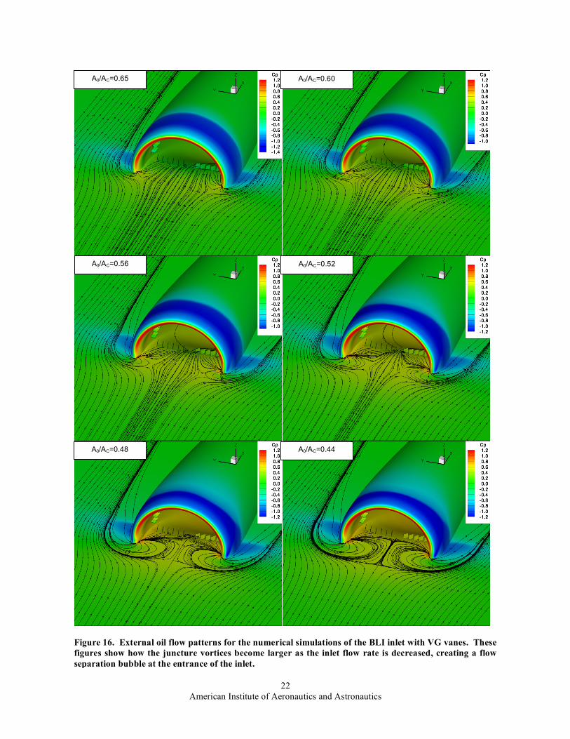
5. External Inlet Flow Figure 16 shows the CFD simulations for various inlet mass flow rates for the BLI inlet with VG vanes on a flat

plate. These figures show the oil flow pattern on the surface of the flat plate ahead of the inlet, which provides an idea of how the flow ahead of the inlet is behaving for A0/AC values ranging from 0.65 to 0.44. The high inlet mass flow rate of 0.65 shows no flow separation ahead of the inlet with some flow reversal as a result of the juncture vortices located where the inlet lip meets the flat plate surface. This figure also shows how the flow is slowing down before entering the inlet and how the flow near the surface moves around the inlet. The figures also show the surface CP contours where there’s a high pressure at the stagnation region on the inlet lip and a low-pressure region on the top of the cowling just ahead of a shock. These figure also show the vanes inside of the inlet. As the mass flow is decreased, the juncture vortices become larger until they meet at the center of the inlet entrance when A0/AC = 0.48 indicating the start of a large separation bubble. These figures also show how the spillage around the inlet is increasing for a decreasing inlet mass flow.

C. BLI Inlet with Jet Flow Control Numerical simulations were performed to match the experimental conditions for a single jet configuration tested

in the wind tunnel experiment. The jet configuration is shown in Fig. 6 where there are 36 total jets with two groups of 18 jets placed symmetrically on each side of the inlet. The simulations were performed at a free-stream Mach


9

number of 0.85 and a constant inlet mass flow ratio of 0.537. Steady-state flow solutions were performed for several jet actuator mass flow rates for the BLI inlet on a flat plate.

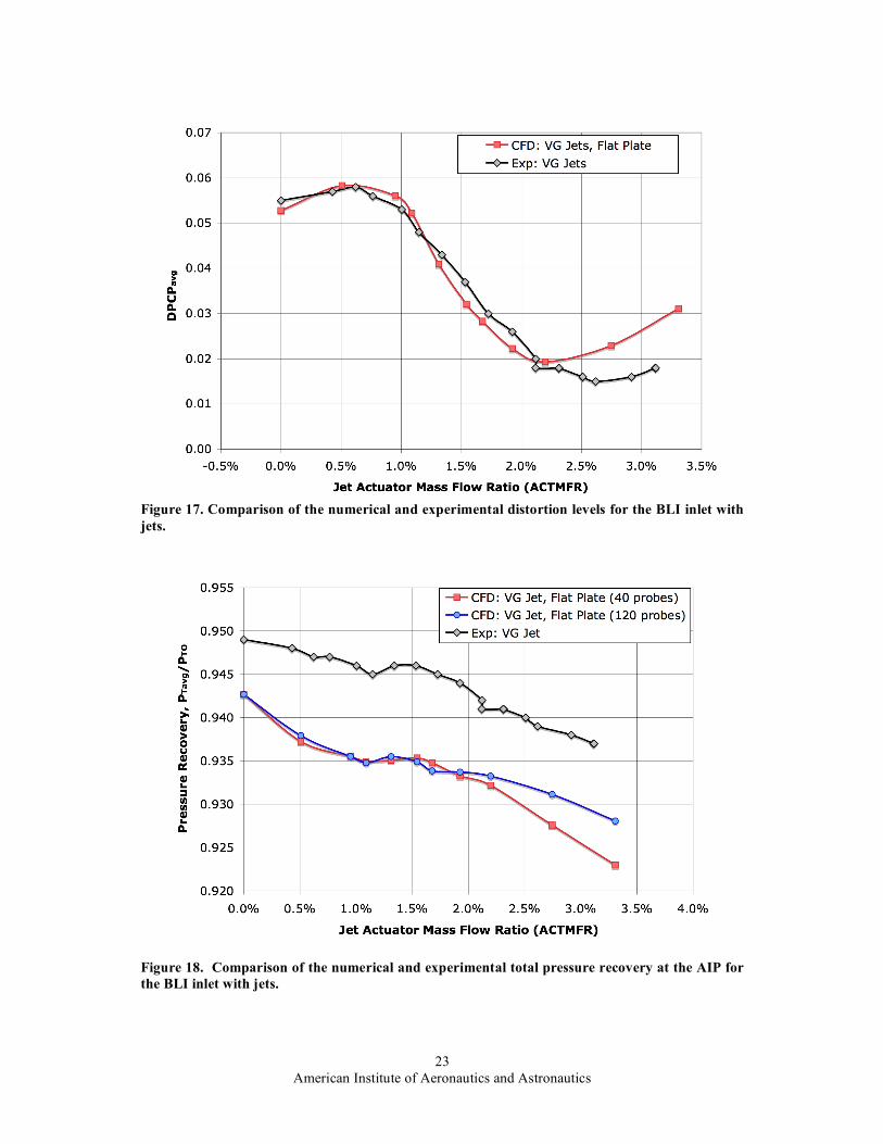
1. Inlet Distortion Figure 17 shows the DPCPavg distortion comparison between the CFD and experiment for several different

actuator mass flow ratios. The total mass flow rate for the jets are reported as a percentage of the inlet mass flow rate and will be referred to as a jet actuator mass flow ratio (ACTMFR). This comparison shows that the numerical simulations compare very well to the experimental data for ACTMFRs below 2.2%. Above an ACTMFR of 2.2% the CFD starts to diverge from the experimental data, predicting a larger flow distortion value. Overall, this jet configuration had a minimum DPCPavg of 0.015 for an actuator mass flow ratio of 2.6% showing the effectiveness of the jets to improve the flow circumferential distortion. Figure 17 also show that the distortion does not start to decrease until an ACTMFR of 1.0% is reached. It is conjectured that this is the point where the forces from the jets balances out the forces from the natural secondary flow generated by the S-shape of the inlet. Above an ACTMFR of 1.0% is where the jets start to redistribute the low momentum from the ingested boundary layer flow.

2. Total Pressure Recovery The inlet total pressure recovery in Fig. 18 shows an offset of 0.01 similar to the baseline and vane comparisons.

This comparison also shows that both the experiment and numerical simulations have a decreasing pressure recovery for an increasing jet mass flow rate. This relation is counterintuitive as one would think that the jets would energize the low-momentum flow increasing the average total pressure at the AIP. Figure 18 also includes a 120-probe total pressure recovery for the CFD simulation. At the highest ACTMFR level the 120-probe rake shows a 0.005 difference when compared to a 40-probe rake resolution with almost no difference below ACTMFR of 2.25%. The 120-probe rake also shows the same trend in the drop of the total pressure recovery for increasing actuator mass flow rate as seen when using the 40-probe rake. This comparison to the 120-probe rake suggests that the total pressure drop for an increasing ACTMFR is not related to the resolution of the rake. It’s possible that the decrease in total pressure recovery is a result of flow separation created by the jets, which becomes larger as the ACTMFR is increased.

3. AIP Total Pressure Ratio Contours Contour plots of the total pressure ratio at the AIP for the numerical and experimental results are shown in Fig.

19. A comparison of the ACTMFR at 1.0% is shown in Fig. 19(a). Figure 17 showed the 1.0% jet mass flow ratio to be the point where the flow distortion starts to decrease with increasing ACTMFR. This contour plot comparison shows a fairly stratified total pressure flow field at the AIP as opposed to the baseline flow in Fig. 10(a) where the low total pressure region has a circular pattern. Taking these two observations into consideration it would appear that the 1.0% jet mass flow ratio is the point where the forces from the jets is equal the forces generated by the natural secondary flow of the S-shaped duct.

By increasing the ACTMFR to 1.7%, the low total pressure flow is now forced up along the sides of the inlet as shown in Fig. 19(b). This comparison of the contour plots show how the CFD has a lower total pressure region on the sides of the AIP as opposed to the experiment. However, the low total pressure region at the bottom of the AIP matches fairly well to the experimental data where the thicknesses of the low total pressure region on the sides of the AIP compare well. While the CFD does have a lower minimum total pressure on the sides of the AIP, the circumferential distortion levels are nearly the same with an average pressure recovery 0.011 lower than the experiment.

Figure 19(c) shows that, as ACTMFR is increased to 2.3%, the low total pressure regions in the CFD simulations become larger and move up higher on the sides of the AIP. The experimental data does show a similar trend of the low total pressure region moving up along the sides of the AIP with a decreasing minimum total pressure. However the CFD is showing a much larger low total pressure region with a lower minimum total pressure level as compared to the experimental measurements. As in the previous mass flow ratio cases, the circumferential distortion level compares very well with the CFD predicting a 0.008 lower total pressure recovery level. The contours still show that the thickness of the low total pressure regions to be about the same size as compared to the experiment where the CFD is starting to show a thinning at the bottom sides of the AIP.

The contour plot of the CFD simulation at an ACTMFR of 2.85% is shown in 19(d). This comparison shows that the CFD does not compare well to the experimental results. The low total pressure regions on the sides of the AIP have become much larger than the experimental measurements. The experiment does indicate the same trend of the low total pressure regions on the sides of the inlet becoming larger with a decreasing minimum total pressure but not the same extent as the CFD simulations. As a result, the DPCPavg values do not compare well for this high ACTMFR case. However, the total pressure recovery levels are becoming closer. The CFD contour plots also show a thinning of the low total pressure regions on at the bottom sides of the AIP with a bulging on the sides that were not observed in the experiment.


10

Overall the comparisons of the contour plots for the jet case show that the CFD is generating a much larger low total pressure region on the sides of the inlet as compared to the experiment. The CFD did show a good prediction of the size of the low total pressure regions and does capture the general trend of flow at the AIP for increasing jet actuator mass flow rates. Further analysis needs to be performed in order to determine why the CFD is predicting a much larger low total pressure region on the sides of the inlet as compared to the experiment. It is speculated that the vortices generated by the jets have merged into a single vortex that forms this large low total pressure region. Comparisons of experimental and computational predictions of vortices submerged in a boundary flow by Allan, Yao, and Lin33 showed that the turbulence models had a tendency to over predict the dissipation rate inside the vortex. This would mean that the vortex generated by the jets in the BLI inlet simulation are dissipating to quickly and may result in the much larger vortex. The other possibility is that the velocity profile at the jet exit does not match the experiment. While the velocity profiles of the jets in the experiment were not measured, the CFD simulations do show a jet with a relatively square velocity profile, which would result in the CFD having higher momentum jets than the actual jets in the experiment.

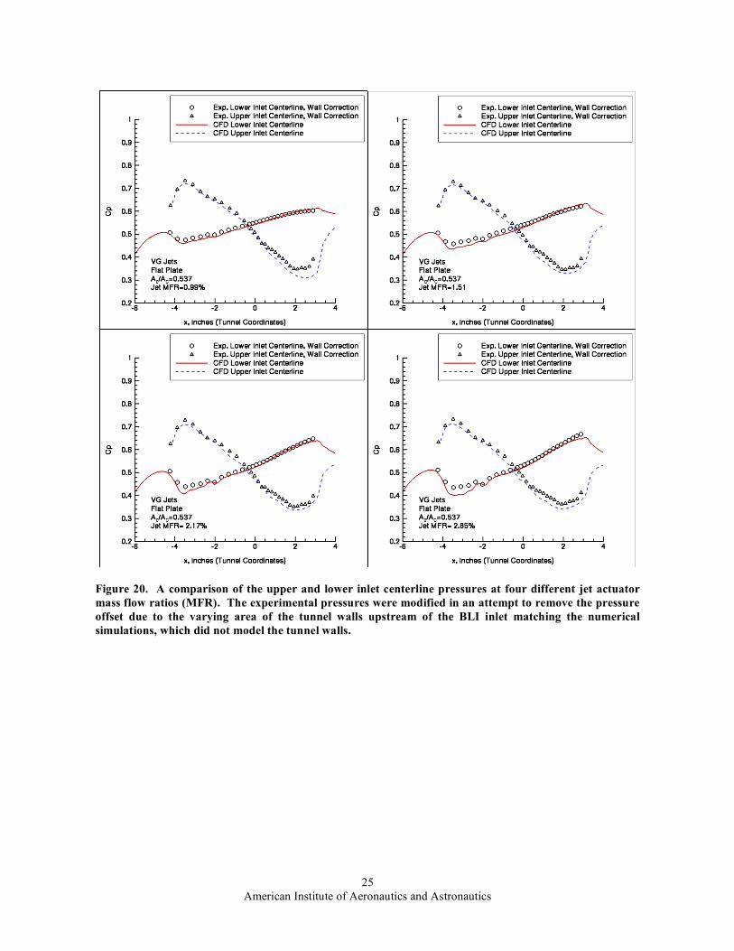
4. Inlet Centerline Surface Pressures Figure 20 shows a comparison of the upper and lower inlet centerline surface pressures inside the inlet for the jet

configuration. The comparison for the ACTMFR of 0.99% shows a very good agreement with the experimental surface pressures. This figure also shows a similar dip in the pressure profile near x = -2 as a result of the jets for both the experiment and CFD profiles. The surface pressures for ACTMFR of 1.51% also compares well to the experiment with little difference to the 0.99% ACTMFR case. There is a slight decrease in the pressure on the lower inlet centerline surface pressure near the jets with a slight increase in the pressure profile as it approaches the AIP. The next comparison shows the surface pressures for an ACTMFR of 2.17% where the CFD is in good agreement with the experimental measurements. This plot also shows the continuing trend of a slight increase in the slope of the bottom centerline surface pressure with an increased dip in the pressure profile at x = -2. This case does show a slight difference near the entrance of the inlet between the CFD and experiment. The high ACTMFR case of 2.85% shows a much more pronounced slope increase in the lower centerline surface pressure profile, which compares well with the experiment. This comparison does show a difference in the centerline pressure at the beginning of the inlet at the location of the jets. Overall the inlet surface pressures agree well with the experiment having some small differences at the higher ACTMFR values.

V. Conclusions This investigation evaluated the ability of a RANS flow solver, OVERFLOW, developed at NASA, to predict

the flow field for a BLI offset inlet in a transonic free-stream flow with and without flow control devices. Numerical simulations were compared to wind tunnel measurements of a BLI offset (S-shaped) inlet test conducted at the NASA Langley 0.3-Meter Transonic Cryogenic Tunnel. The numerical simulations were compared to the BLI inlet experimental data at a free-stream Mach number of 0.85 and an average Reynolds number of 2 million based on the length of the fan-face diameter. Comparisons of inlet flow distortion, pressure recovery, and inlet wall pressures were made between the CFD and the experiment. Numerical simulations with the wind tunnel walls were also performed in order to determine the influence of the walls on the internal inlet flow field for the baseline and vane cases.

1. Baseline BLI Inlet The baseline comparisons of the BLI inlet showed that the RANS flow solver agreed very well with the

experimental results. A comparison of the circumferential distortion descriptor, DPCPavg, showed that the flow solver could predict the distortion levels very well in the operational inlet mass flow range. Below the operational inlet mass flow ratio of A0/AC = 0.46, the numerical simulations started to diverge from the experimental results, predicting a higher distortion values. This difference was associated with the development of a flow separation bubble at the entrance of the inlet and the ability of the flow solver to predict the correct size and character of the flow separation region. Comparison of the total pressure recovery showed that the flow solver under predicted the total pressure recovery with a 0.01 offset for A0/AC values above 0.44. The total pressure recovery for the CFD did predict the correct trend of decreasing total pressure recovery with decreasing inlet mass flow for inlet mass flows in the operational range of the inlet. At an inlet mass flow ratio of 0.46, the numerical simulations showed a rapid decrease in the total pressure recovery for decreasing inlet mass flow ratios, which was seen to start at 0.37 in the experiment. This indicated that significant flow separation at the entrance of the inlet was occurring at a higher inlet mass flow ratio for the CFD as compared to the experiment. Comparisons of the inlet centerline surface pressures show good agreement between the numerical simulations and the experiment in the operational inlet mass flow


11

range. A comparison of the total pressure ratio contour plots also show that the numerical simulations were able to predict flow pattern well with a good prediction of the minimum total pressure region.

2. BLI Inlet with Passive Vane Flow Control A wind tunnel experiment with passive VG vanes inside the BLI inlet was performed and compared to numerical

simulations to evaluate the ability of the RANS flow solver to predict the internal flow with this type of passive flow control device. Overall the numerical simulations were able to capture the correct trends for the circumferential distortion but had distortion levels that were approximately twice the levels measured in the experiment. This large difference was associated to the sensitivity of DPCPavg to the symmetry of the flow field at the AIP using the 40-probe rake for this vane case. This sensitivity is the result of a low total pressure region, which is between the 40-probe rake arms coupled with the fact that the flow near the centerline of the AIP generates the largest circumferential distortion. An asymmetry in the inlet flow moves these regions in and out of view of the rake probes, significantly changing the distortion levels. It was also discovered after testing of the vane configuration that the side vanes were not placed symmetrically inside the inlet model, creating an asymmetric flow pattern. It is believed that this asymmetry in the vane installation was one of the main sources for the large difference seen in the circumferential distortion levels between the CFD and the experiment. While the CFD forced the flow to be symmetrical about the inlet centerline, a full inlet simulation, with the exact vane location, could be performed to verify the claim that the asymmetry of the vanes was indeed the main source of the difference in the DPCPavg distortion values.

The pressure recovery levels were predicted very well for the operation range of the inlet and showed a significant decrease by the CFD, as compared to the experiment, below an A0/AC of 0.45. A rake resolution comparison was made using the CFD data showing that a 120-probe rake would have a pressure recovery 0.005 lower than the 40-probe rake. This was a result of the 40-probe rake missing the narrow low total pressure region at the top of the AIP in-between the rake arms, which decreases the average total pressure recovery value.

A comparison of the internal inlet centerline pressures shows good agreement between the CFD and experiment. The CFD did show an under prediction of the suction peak on the bottom of the inlet generated by the vanes. The contour plots of the total pressure ratio compared well with the experiment showing a slightly larger low-pressure region at the bottom of the AIP. The numerical simulations showed a small low total pressure region at the top of the AIP on both sides of the centerline that could not be detected by the 40-probe rake used in the experiment. The contours at the AIP also started to significantly differ at very low inlet mass flow rates, outside the operational range of the inlet, where the flow separation at the entrance of the inlet starts to dominate the inlet flow.

3. BLI Inlet with Jet Flow Control Numerical simulations of a single jet configuration were compared to experimental data for varying actuator

mass flow rates at a fixed inlet mass flow ratio. The DPCPavg levels compare well for actuator mass flow ratio below 2.2% of the inlet flow. Above an actuator mass flow ratio of 2.2%, the circumferential distortion values for the CFD start to become larger than the distortion levels measured in the experiment. This was the result a two large low total pressure regions on the side of the inlet AIP predicted by the numerical simulations but not seen in the experimental data. The flow solver also under predicted the total pressure recovery, which had an average offset of 0.01, which was also seen in the baseline case. Despite this offset, the CFD was able to capture the trend of decreasing total pressure recovery with increasing actuator mass flow rate. This trend was counterintuitive and is conjectured to be a result of the jets producing a local flow separation, decreasing the average total pressure recovery at the AIP.

The AIP contours compared well for actuator mass flow ratios below 2.0% of the inlet mass flow with a lower minimum total pressure values on the sides of the AIP predicted by the CFD but not seen in the experiment. At the higher jet mass flow ratios; the CFD was predicting a much larger low total pressure region on the sides of the AIP as compared to the experiment. It’s not known why the CFD is predicting these large low total pressure regions for these high actuator mass flow rates. One possible reason is that the dissipation rate generated by the turbulence model is too large for the vortices generated by the jets, creating a much larger vortex. Another possibility is that the jet velocity profiles in the CFD simulations are not the same as the experiment where the CFD may have much more square velocity profile thus creating higher momentum jets with stronger streamwise vortices.

Acknowledgements This research was supported by the NASA UEET Highly Integrated Inlet project office. All of the numerical

simulations were performed on the NAS Columbia SGI Altix supercomputer. A special thanks to Mr. Bobby Berrier for his guidance on testing flush-mounted, boundary layer ingesting inlets. The authors would also like to


12

thank Ms. Susan Gorton for her leadership and support during this research project and Dr. Pieter Buning for his discussions and support of the numerical flow solutions.

References 1Brown, A. S., “HSR Work Propels UEET Program (High Speed Research in Ultraefficient Engine Technology in Aircraft

Industry),” Aerospace America, Vol. 37, No. 5, May 1999, pp. 48-50. 2Liebeck, R. H., “Design of the Blended-Wing-Body Subsonic Transport,” AIAA 2002-002. 3Berrier, B. L. and Allan, B. G., “Experimental and Computational Evaluation of Flush-Mounted, S-Duct Inlets,” AIAA

Paper 04-0764, January 2004. 4Gorton, S. A., Owens, L. R., Jenkins, L. N., Allan, B. G., and Schuster, E. P., “Active Flow Control on a Boundary-Layer-

Ingesting Inlet,” AIAA Paper 04-1203, January 2004. 5Anabtawi, A. J., Blackwelder, R. F., Lissaman, P. B. S., and Liebeck, R. H., “An Experimental Investigation of Boundary

Layer Ingestion in a Diffusing S-Duct With and Without Passive Flow Control,” AIAA Paper 99-0739. 6Allan, B. G., Owens, L. R., and Berrier, B. L., “Numerical Modeling of Active Flow Control in a Boundary Layer Ingesting

Offset Inlet,” AIAA Paper 04-2318. 7Taylor, H. D., “Application of Vortex Generator Mixing Principle to Diffusers. Concluding Report,” United Aircraft Corp.

Research Dept., Rep. R-15064-5, East Hartford, CT, Dec. 1948. 8Grose, R. M., and Taylor, H. D., “Theoretical and Experimental Investigation of Various Types of Vortex Generators,”

United Aircraft Corp. Research Dept., Rep. R-15362-5, East Hartford, CT, March 1954. 9Valentine, E. F. and Carrol, R. B., “Effects of Some Arrangements of Rectangular Vortex Generators on the Static Pressure

Rise Through a Short 2:1 Diffuser,” NASA RM L50L04, Feb. 1951. 10Valentine, E. F. and Carrol, R. B., “Effects of Some Primary Variables of Rectangular Vortex Generators on the Static

Pressure Rise Through a Short Diffuser,” NASA RM L52B13, May 1952. 11Pearcy, H. H. and Stuart, C. M., “Methods of Boundary-Layer Control for Postponing and Alleviating Buffeting and other

Effects of Shock-Induced Separation,” Presented at the IAS National Summer Meeting, Los Angles, CA, June, 1959. 12Kaldschmidt, G., Syltedo, B. E. and Ting, C. T., “727 Airplane Center Duct Inlet Low-Speed Performance Confirmation

Model Test for Refanned JT8D Engines – Phase II,” NASA CR-134534, Nov. 1973. 13Anderson, B. H. and Levy, R., “A Design Strategy for the Use of Vortex Generators to Manage Inlet-Engine Distortion

Using Computational Fluid Dynamics”, NASA/TM-1991-104436, June 1991. 14Hamstra, J. W., Miller, D. N., Truax, P. P., Anderson, B. H., and Wendt, B. J., “Active Inlet Flow Control Technology

Demonstration,” The Aeronautical Journal of the Royal Aeronautical Society, October, 2000. 15Anderson, B. H. and Keller, D. J., “Robust Design Methodologies for Optimal Micro-Scale Secondary Flow Control in

Compact Inlet Diffusers”, NASA/TM-2001-211477, March 2001. 16Anderson, B. H., Baust, H. D., and Agrell, J., “Management of Total Pressure Recovery, Distortion and High Cycle Fatigue

in Compact Air Vehicle Inlets,” NASA TM-2002-212000, December, 2002. 17Anderson, B. H. and Keller, D. J., “Optimal Micro-Scale Secondary Flow Control for the Management of HCF and

Distortion in Compact Inlet Diffusers”, NASA/TM-2002-211686, July 2002. 18Anderson, B. H., Baust, H. D., and Agrell, J., “Management of Total Pressure Recovery, Distortion and High Cycle Fatigue

in Compact Air Vehicle Inlets,” NASA TM-2002-212000, Dec. 2002. 19Anderson, B. H. and Keller, D. J., “A Robust Design Methodology for Optimal Micro-Scale Secondary Flow Control in

Compact Inlet Diffusers”, AIAA Paper No. 2002-0541, Jan. 2002. 20Anderson, B. H., Miller, D. N., Addington, G. A., and Agrell, J., “The Role of Robust Optimization in Managing Flow in

Compact Air Vehicle Inlets,” NASA TM-2003-212017, Jan. 2003. 21Anderson, B. H., Miller, D. N., Marvin, G. C., and Agrell, J., “The Role of Design-of-Experiments in Managing Flow in

Compact Air Vehicle Inlets,” NASA TM-2003-212601, Sept. 2003. 22Anderson, B. H., Miller, D. N., Addington, G. A., and Agrell, J.,” Optimal Micro-Vane Flow Control for Compact Air

Vehicle Inlets,” NASA TM-2004-212936, Feb. 2004. 23Anderson, B. H., Miller, D. N., Addington, G.A., and Agrell, J.,” Optimal Micro-Jet Flow Control for Compact Air Vehicle

Inlets,” NASA TM-2004-212937, Feb. 2004. 24Anderson, B. H., Miller, D. N., Yagle, P.J., and Truax, P.P., “A Study on MEMS Flow Control For the Management of

Engine Face Distortion in Compact Inlet Systems,” Proceedings of the 3rd ASME/JSME Joint Fluids Engineering Conference, July, 1999.

25Bobby L. Berrier and Melissa B. Morehouse, Evaluation of Flush-Mounted, S-Duct Inlets With Large Amounts of Boundary Layer Ingestion , NATO/RTA Symposium on Vehicle Propulsion Integration, Warsaw, Poland, October 6-9, 2003.

26Owens L. R., Allan B. G., and Gorton, S. A., “Boundary-Layer-Ingesting Inlet Flow Control,” AIAA Paper 2006-0839, Jan. 2006.

27Allan, B. G., Owens L. R., and Lin, J. C., “Optimal Design of Passive Flow Control for a Boundary-Layer-Ingesting Offset Inlet Using Design-of-Experiments,” AIAA Paper 2006-1049, Jan. 2006.

28Buning, P. G., Jespersen, D. C., Pulliam, T. H., Klopfer, W. M., Chan, W. M., Slotnick, J. P., Krist, S. E., and Renze, K. J., “OVERFLOW User’s Manual Version 1.8m,” Tech. Rep., NASA Langley Research Center, 1999.


13

29Jespersen, D. C., Pulliam, T. H., and Buning, P. G., “Vortex Generator Modeling for Navier-Stokes Codes,” AIAA 97-0644, 1997.

30Pulliam, T. H. and Chaussee, D. S., “A Diagonal Form of an Implicit Approximate-Factorization Algorithm,” Journal of Computational Physics, Vol. 39, February 1981, pp. 347–363.

31Steger, J. L., Dougherty, F. C., and Benek, J. A., “A Chimera Grid Scheme,” Advances in Grid Generation, edited by K. N. Ghia and U. Ghia, Vol. 5 of FED, ASME, New York, NY, 1983.

32Menter, F., “Improved Two-Equation Turbulence Models for Aerodynamic Flows,” Tech. Rep. TM 103975, NASA, NASA Langley Research Center, Hampton, VA 23681-2199, 1992.

33Allan, B. G., Yao, C. S., and Lin, J. C., “Numerical Simulations of Vortex Generator Vanes and Jets on a Flat Plate,” AIAA Paper 02–3160, June 2002.

34Murphy, K., Buning, P., Pamadi, B., Scallion, W., and Jones, K., “Status of Stage Separation Tool Development for Next Generation Launch Technologies,” AIAA paper 04–2595, June 2004.

35Chan, W. M. and Gomez, R. J., “Advances in Automatic Overset Grid Generation Around Surface Discontinuities,” AIAA Paper 99–3303, July 1999.

36Gas Turbine Engine Inlet Flow Distortion Guidelines. Aerospace Recommended Practice 1420B, SAE International, 2001.

Figure 1. Overset grids for VG vanes inside the BLI inlet.

Figure 2. Close-up view of the overset nozzle grids for a VG jet inside the BLI inlet.

Figure 4. Side view of the overset grids on the centerline of the inlet.

Figure 3. View of the overset nozzle grids and inlet grids.


14

Figure 6. Jet configuration used in this investigation. This figure shows the inlet half with the jet actuator configuration used in the comparison with the experiment. This configuration has a total of 36 jets with 18 jets placed symmetrically about the inlet centerline.

Figure 5. VG vane configuration for BLI inlet wind tunnel experiment. This figure shows a cross section view of the vane layout with the vane size and angle-of-attack. This figure also shows a 3D view of the inlet half depicting the location of the vanes relative to the inlet geometry.


15

Figure 7. Comparison of the numerical and experimental baseline inlet distortion levels, DPCPavg, at a free-stream Mach number of 0.85 at a ReD=3.5 million for the experiment and 2.2 million for the numerical simulations.

Figure 8. Comparison of the numerical and experimental baseline inlet total pressure recovery levels at a free-stream Mach number of 0.85 at a ReD=3.5 million for the experiment and 2.2 million for the numerical simulations.


16

Figure 9. Contour plots of the Mach number for the baseline inlet flow at the centerline of the BLI inlet. These figures show the generation of a flow separation bubble at the entrance of the inlet for deceasing inlet mass flow rates.


17

(a)

(b)

(c)

(d) Figure 10. A comparison of the numerical and experimental results for the baseline BLI inlet at four different A0/AC mass flow ratios. The numerical results are for the BLI inlet on a flat plate.


18

Figure 11. A comparison of the inlet centerline pressures on the top and bottom of the BLI inlet at four different mass flow ratios. The experimental pressures were modified in an attempt to remove the pressure offset due to the varying area of the tunnel walls upstream of the BLI inlet matching the numerical simulations, which did not model the tunnel walls.


19

Figure 12. Comparison of the numerical and experimental distortion for the inlet with VG vane flow control.

Figure 13. Comparison of the numerical and experimental total pressure recovery at the AIP for the inlet with VG vane flow control.


20

(a)

(b)

(c)

(d) Figure 14. A comparison of the numerical and experimental results for the BLI inlet at three different AOAC mass flow ratios. The numerical results are for the BLI inlet on a flat plate.


21

Figure 15. The upper and lower inlet centerline pressures for the BLI inlet with VG vanes at four different inlet mass flow rates. The experimental pressures were modified in an attempt to remove the pressure offset due to the varying area of the tunnel walls upstream of the BLI inlet matching the numerical simulations, which did not model the tunnel walls.


22

Figure 16. External oil flow patterns for the numerical simulations of the BLI inlet with VG vanes. These figures show how the juncture vortices become larger as the inlet flow rate is decreased, creating a flow separation bubble at the entrance of the inlet.

A0/AC=0.65 A0/AC=0.60

A0/AC=0.56 A0/AC=0.52

A0/AC=0.48 A0/AC=0.44


23

Figure 18. Comparison of the numerical and experimental total pressure recovery at the AIP for the BLI inlet with jets.

Figure 17. Comparison of the numerical and experimental distortion levels for the BLI inlet with jets.


24

(a)

(b)

(c)

(d) Figure 19. Comparisons of the numerical and experimental results for the BLI inlet with jets at four different jet actuator mass flow ratio and a fix AO/AC. The numerical results are for the BLI inlet on a flat plate where the CFD results are interpolated onto the 40 probe rake locations as was measured in the experiment.


25

Figure 20. A comparison of the upper and lower inlet centerline pressures at four different jet actuator mass flow ratios (MFR). The experimental pressures were modified in an attempt to remove the pressure offset due to the varying area of the tunnel walls upstream of the BLI inlet matching the numerical simulations, which did not model the tunnel walls.

numerical modeling of flow control in a boundary-layer- ingesting offset inlet ... ·...

Documents