numerical simulation of a guitar - accueil - ensta paris
TRANSCRIPT
HAL Id: hal-00982757https://hal-ensta-paris.archives-ouvertes.fr//hal-00982757
Submitted on 12 Mar 2018
HAL is a multi-disciplinary open accessarchive for the deposit and dissemination of sci-entific research documents, whether they are pub-lished or not. The documents may come fromteaching and research institutions in France orabroad, or from public or private research centers.
L’archive ouverte pluridisciplinaire HAL, estdestinée au dépôt et à la diffusion de documentsscientifiques de niveau recherche, publiés ou non,émanant des établissements d’enseignement et derecherche français ou étrangers, des laboratoirespublics ou privés.
Numerical simulation of a guitarEliane Bécache, Antoine Chaigne, Grégoire Derveaux, Patrick Joly
To cite this version:Eliane Bécache, Antoine Chaigne, Grégoire Derveaux, Patrick Joly. Numerical simulation of a guitar.Computers and Structures, Elsevier, 2005, Advances in Analysis of Fluid Structure Interaction, 83(2-3), pp.107-126. �10.1016/j.compstruc.2004.04.018�. �hal-00982757�

NUMERICAL SIMULATION OF A GUITAR
ELIANE BECACHE∗, ANTOINE CHAIGNE† , GREGOIRE DERVEAUX∗ ‡ , AND PATRICK
JOLY∗
Abstract.The purpose of this study is to present a time-domain numerical modeling of the guitar. The
model involves the transverse displacement of the string excited by a force pulse, the flexural motionof the soundboard and the sound radiation in the air. We use a specific spectral method for solvingthe Kirchhoff-Love’s dynamic plate model for orthotropic material, a fictitious domain method forsolving the fluid-structure interaction and a conservative scheme for the time discretization. Oneof the originality of the proposed scheme is a stable coupling method between a continuous timeresolution and a discrete one.
Key words. Kirchhoff-Love’s plate model, fluid-structure interaction, mixed finite elements,fictitious domain method, spectral method, energy method, stability.
AMS subject classifications. 65M12, 65M60, 65M70.
1. Introduction. The purpose of the presented study is the numerical resolu-tion of a physical modeling of the acoustic guitar. This work is part of the generalframework time domain modeling of musical instruments initiated about 10 years agoby A. Chaigne, which purpose is to better understand the vibroacoustical behavior ofinstruments by use of an accurate physical modeling and advanced numerical methods.The interest of the time-domain approach instead of the more usual frequency-domainapproach, is the accuracy in the modeling of the coupling between the different partsof the instrument. Such a model constitutes a virtual instrument in which it is possibleto change easily the geometrical or physical parameters. It will thus be of great helpto develop tools for instrument making, sound recording or psychoacoustic studies.Among other works realized in this general framework, we can mention the modelingof the damping in the guitar top plate made by Chaigne and Lambourg [10] and thenumerical modeling of the timpani [37].
The instrument is considered as a set of simple structures which are coupledto each other. Since we wish to focus on the modeling of the soundboard and onthe fluid-structure interaction, the model used for the other parts of the instrument isintentionally kept simple. An idealized plucking force is acting on a 1D damped stringmodel. The string is coupled to the soundboard via the bridge. The soundboardis modeled as an orthotropic heterogeneous damped Kirchhoff-Love plate, with asoundhole, clamped at its boundaries. The other parts of the body (back, neck,sides...) are assumed to be perfectly rigid. The plate radiates both inside the cavityand in the external free field. The modeling of the complete 3D sound field is a newapproach comparing to almost all previous works on the guitar, where the cavity istaken into account as a simple oscillator.
The well posedness of the model is shown with the help of the Hille-Yosida theo-rem. One of the main difficulty raised by its numerical resolution is that the domainof computation for the sound radiation is a 3D unbounded domain, which involve thecomplex geometry of the guitar. In addition, a guitar sound can last up to 6 seconds,so that the number of iterations may be great (typically 300,000 time steps for 6s
∗Inria Roquencourt, Projet Ondes, 78153 Le Chesnay Cedex, France.
†Ensta-UME, Chemin de la Huniere, 91761 Palaiseau Cedex. France
‡Mathematic Department, Stanford University. Email: [email protected]
1

of sound). It is thus of great importance to define an efficient resolution scheme. Inorder to circumvent these difficulties, the fluid-structure interaction problem is solvedwith the help of a fictitious domain method which main interest is to allow the useof a regular mesh for the approximation of the acoustic field while the geometry ofthe instrument is taken into account with an accurate triangular surface mesh. Forthe time discretization, conservative centered finite differences are used. To simulatethe free space, the computations are restricted to a box of finite size with the help ofhigher oder absorbing boundary conditions.
Another important difficulty to cope with this model is the resolution of theKirchhoff-Love’s dynamic plate equation which includes a fourth order space operatorand is intrinsically dispersive, which complicates both space and time discretization.We have chosen to solve it with a spectral method, which is particularly efficientin the case of a great number of iterations: the eigenmodes are calculated with anon standard higher order mixed finite elements method, based on a velocity-momentformulation and the spatial semi-discretized problem is solved analytically in time.
The string equation is solved using standard mixed finite elements of lower orderon a regular mesh and explicit centered finite differences are used.
The stability of the coupled scheme is ensured through a discrete energy identity.In this aim, the spatial discretization of the equations of the model is based on amixed variational formulation of the complete system. The time stepping is chosen insuch a way that almost all computations, and in particular the 3D computations, areexplicit. The resolution of the scheme involves only the inversion at each time stepof a small sparse symmetric positive matrix which arises from the fictitious domainresolution of the fluid-structure interaction.
The main originality of the proposed scheme is certainly that it is a stable couplingmethod between a continuous time resolution (for the plate) and a discrete one (forthe string and the air). In addition, the two stability conditions of the completescheme are exactly the same than the usual CFL conditions obtained for the standardfinite difference discretization of the uncoupled 1D and 3D wave equation. This resultshows the robustness of the coupling scheme.
The paper is organized as follow: section 2 is devoted to the description of theguitar and the presentation of the model. Section 3 presents the main results of themathematical analysis of this model: well-posedness and energy identity of the con-tinuous problem. Since it is solved with a spectral method whereas all other equationsare solved with finite elements in space and finite differences in time, the numericalresolution of the plate equation takes a particular place and is thus presented in sec-tion 4. The numerical scheme of the complete problem is then presented in details insection 5. The well-posedness of this scheme and the stability analysis are discussedin section 6 and finally in section 7, numerical results are given.
2. The model.
2.1. Description of the guitar. The body of guitar is made up of the sound-board, the sides, the back and the neck. The 6 string are attached on one side tothe neck and on the other side to the bridge. The soundboard itself is a thin woodenlayer containing a sound hole and reinforced by struts (pieces of hard wood glued onits internal face which have a great influence on the shape of the structural modesof the soundboard and on the radiation efficiency of the guitar [39, 35]). The soundproduced by a string is appreciated since antiquity for its natural harmonic properties.Unfortunately, this sound is practically inaudible because of its very small diameter.The vibrations of the string are thus transmitted to the soundboard, which large area
2

ensures efficient coupling to the air. In addition, the soundboard is itself coupled toan acoustic cavity pierced by a hole in order to reinforce the sound power in the lowfrequency range, by the help of the Helmholtz resonance frequency [40, 23].
The following assumptions were made in order to propose a physical modeling ofthe instrument:
• the amplitudes of vibration are small, which justify a linear model,• the body has no thickness and the neck is neglected,• only the soundboard vibrate (the rest of the body is supposed perfectly rigid),• the soundboard is modeled using a Kirchhoff-Love flexural plate equation
(the motion parallel to the medium plan is neglected). The struts and thebridge are considered as heterogeneities,
• only the transverse polarization of the string is considered: the in-plane dis-placement of the string (parallel to the soundboard) is neglected,
• the string is excited with an idealized plucking force,• the internal phenomena of damping in the plate and in the string are modeled
by dissipative terms of viscoelastic type.Geometrical description. The body of the guitar is delimited by a surface denoted
Γ which is divided into two parts: Γ = ω∪Σ, where ω is the top plate of the instrumentand Σ is the rest of the surface (ie. sides and back). The boundary of ω itself isdivided into two parts: γ0 is the outer boundary of the top plate and γf is the innerboundary, along the hole. The surrounding air occupies the domain Ω = R
3� Γ. The
string of length ls is rigidly fixed to the neck at a point denoted O, chosen as originof the coordinate system (see Fig. 2.1).
�
��
���
���
��� �
�
���
��� ��� �
� � ����� �
�
Fig. 2.1. Geometrical description of the guitar
Unknowns. This model includes the following unknowns, all time dependent:• the vertical displacement of the string us(x, t), x ∈]0, ls[;• the vertical displacement of the soundboard up(x, y, t), (x, y) ∈ ω :• the acoustic pressure p(x, y, z, t), (x, y, z) ∈ Ω;• the acoustic velocity field va(x, y, z, t), (x, y, z) ∈ Ω.
Notations. A simple underlined quantity (e.g. θ) denotes a vector in R2, a
double underlined quantity (e.g. M ) denotes a tensor of second order in R2 and a
bold simple underlined quantity (e.g. N) denotes a vector in R3. div denotes the
usual divergence operator for vectors and ∇ denotes the usual gradient operator for
3
scalars. Div denotes the divergence operator for tensors defined by:
DivM =
(∂1M11 + ∂2M12
∂1M21 + ∂2M22
)
ε (θ) denotes the plane linearized strain tensor of the vector field θ, defined by:
εαβ(θ) =12(∂βθα + ∂αθβ), ∀α, β ∈ {1, 2}.
2.2. Equations. This model of guitar is described by the following set of equa-tions:
Equations for the string:
(2.1)
⎧⎪⎪⎪⎪⎪⎪⎨⎪⎪⎪⎪⎪⎪⎩
(a) ρs∂2us
∂t2− T (1 + ηs
∂
∂t)∂2us
∂x2= fs(x, t), in ]0, ls[,
(b) us(0, t) = 0, ∀t > 0,
(c) us(ls, t) =∫
ω
G(x, y)up(x, y, t)dxdy, ∀t > 0.
Equations for the soundboard :
(2.2)
⎧⎪⎪⎪⎪⎪⎪⎪⎪⎪⎪⎪⎪⎨⎪⎪⎪⎪⎪⎪⎪⎪⎪⎪⎪⎪⎩
(a) aρp∂2up
∂t2+ div DivM = −[p]
ω+ F(x, y, t) in ω,
(b) M = a3C (1 + ηp∂
∂t)ε (∇up) in ω,
(c) F(x, y, t) = G(x, y)T (1 + ηs∂
∂t)∂us
∂x(ls, t) in ω,
(d) up = 0 and ∂nup = 0, on γ0,
(e) (Mn).n = 0 and (DivM ).n + ∂τ [(Mn).τ ] = 0, on γf .
Equations for the surrounding air:
(2.3)
⎧⎪⎪⎪⎪⎪⎪⎪⎨⎪⎪⎪⎪⎪⎪⎪⎩
(a) ρa∂va
∂t+ ∇p = 0, in Ω,
(b) μa∂p
∂t+ div va = 0, in Ω,
(c) va(x, y, 0, t).ez = up(x, y, t), ∀(x, y) ∈ ω,
(d) va(x, y, z, t).N = 0, ∀(x, y, z) ∈ Σ.
At the origin, the whole system is at rest. These initial conditions will be systemat-ically omitted in the following. The previous set of equations ((2.1), (2.2), (2.3)) isdenoted Pg and is described below.
• (2.1a) is the 1D wave equation describing the displacement of the string. T isthe uniform tension, ρs is the uniform lineic density. ηs is an internal dissi-pative term of viscoelastic type. On the right hand side, the force fs exertedby the finger is assumed to be an imposed force fs(x, t) = g(x)h(t), where the
4

C1 function h(t) represents a simple idealized version of the “stick-slip” mech-anism that governs the interaction between string and finger (Fig. 2.2a). Thisforce is distributed over a small segment of the string by means of the smoothpositive function g, normalized so that
∫ ls0
g(x)dx = 1 (Fig. 2.2b). Despite itssimplicity, this excitation is in fairly good agreement with experiments [9].
0
0.2
0.4
0.6
0.8
1
0 0.005 0.01 0.015 0.02
h(t)
(N)
t
(a)
0
0.2
0.4
0.6
0.8
1
0 0.1 0.2 0.3 0.4 0.5 0.6
g(x)
x
(b)
Fig. 2.2. Idealized plucking force. (a) Time dependence. (b) Space dependence
• (2.1b) expresses that the string is fixed at the neck and (2.1c) expresses thatthe string and the soundboard are always in contact at the bridge. Themotion of the string at the bridge is thus given by the mean displacement ofa small plate’s area. G is positive and normalized so that
∫ω G = 1
• (2.2a) is the Kirchhoff-Love equation describing the flexural displacement ofthe soundboard [20, 13, 33]. a = a(x, y) is the thickness and ρp = ρp(x, y)the density. On the right hand side, the force exerted by the surrounding airis [p]
ω= pe − pi, the pressure jump across the soundboard, where pe and pi
denotes the external and internal pressure respectively and F is force exertedby the string (see below).
• (2.2b) is the analogous of Hooke’s law for a Kirchhoff-Love’s plate. M de-notes the bending moment. It is a symmetric tensor of second order. ηp isa uniform dissipative term of viscoelastic type. C = C (x, y) is the rigiditytensor for orthotropic materials. C can be written:
(2.4) C = c11
⎛⎝ 1 c12 0
c12 c22 00 0 c33
⎞⎠ = c11C ,
where c11 is an elastic coefficient in Pa and c12, c22 and c33, are dimensionlesscoefficient. C is supposed to satisfy: 0 < c−
∣∣M ∣∣2 ≤ CM : M ≤ c+∣∣M ∣∣2
• The force F exerted by the string on the plate is assumed to be the normalcomponent of the tension of the string at this point (this is a common as-sumption [23]). This force is distributed over the small plate’s area defined bythe spatial window G used above. For a non dissipative string, consideringsmall displacements, it is given by:
(2.5) F(x, y, t) ≈ −T∂xus(ls, t)G(x, y),
One should modify this last equation in order to take into account the vis-coelastic dissipation in the string, which leads to (2.2c).
5

• The conditions (2.2d) express that the plate is clamped along its outer bound-ary γ0, while the conditions (2.2e) express that the plate is free along thesoundhole γf . n denotes the outer normal and τ denotes the tangentialvector along the boundary δω. ∂n and ∂s denote the normal and tangentialderivative operator along the boundary δω respectively.
• (2.3a) and (2.3b) are the linearized Euler’s equations for the acoustic field.ρa is the density of the air and μa = 1
ρac2a
is the permitivity of the air whereca is the speed of sound in the air.
• (2.3c) expresses the continuity of the normal component of the acoustic ve-locity on ω, which is the standard fluid-structure interaction condition and(2.3d) expresses that the rest of the body is perfectly rigid. N denotes theouter normal to the boundary Σ.
3. Mathematical analysis. It is not difficult to show that the problem Pg iswell posed. In fact, the proof of the Hille-Yosida theorem’s hypothesis [42] is longbut straightforward. One should only take care to the treatment of the free boundaryconditions of the soundboard which must be seen in a weak way [17]. One has:
Theorem 3.1 (Well posedness of the problem Pg). The plucking of the string issupposed to satisfy:
fs ∈ C1(R+, L2(]0, ls[)),
then problem Pg admits a unique strong solution (us, up, p,va) such that:
(3.1)
⎧⎪⎪⎪⎪⎪⎪⎪⎪⎪⎪⎪⎪⎪⎪⎪⎪⎨⎪⎪⎪⎪⎪⎪⎪⎪⎪⎪⎪⎪⎪⎪⎪⎪⎩
us ∈ C2(R+, L2(]0, ls[)) ∩ C1(R+,Vs),[(1 + ηs
∂
∂t)∂2us
∂x2
]∈ C0(R+, L2(]0, ls[)),
up ∈ C2(R+, L2(ω)) ∩ C1(R+,Vp),[(1 + ηp
∂
∂t) div Div C ε (∇up)
]∈ C0(R+, L2(ω)),
p ∈ C1(R+, L2(Ω)) ∩ C0(R+, H1(Ω)),
va ∈ C1(R+, (L2(Ω))3) ∩ C0(R+, H(div, Ω)),
with Vs ={us ∈ H1(]0, ls[) ; us(0) = 0
}and Vp =
{up ∈ H2 ; up = ∂nup = 0 on γ0
}.
The boundary conditions are verified in the following sense:
(3.2)
∣∣∣∣∣∣∣∣∣∣∣∣∣∣∣
us(ls, t) =∫
ω
G(x, y)up(x, y, t)dxdy, in C1(R+, R),⎧⎪⎪⎨⎪⎪⎩
∀u∗p ∈ Vp, (1 + ηp
∂
∂t)∫
ω
div Div C ε (∇up)u∗p
= (1 + ηp∂
∂t)∫
ω
C ε (∇up) : ε (∇u∗p), in C0(R+, R),
va · N =∂up
∂t, in C0(R+, H− 1
2 (Γ)),
where the extension of∂up
∂tto Γ is defined by: (
∂up
∂t)|ω =
∂up
∂t, and (
∂up
∂t)|Σ = 0.
This result is based essentially on the following energy identity, which shows thatthe energy of the complete system decreases with time, when it is free oscillating. It is
6

of particular interest for obtaining a priori estimates of the solution given in Theorem3.1. Furthermore a similar identity will be exploited for ensuring the stability of thenumerical resolution scheme.
Theorem 3.2 (Energy identity). The unique strong solution (us, up, p,va) ofproblem Pg satisfies:
(3.3)dE
dt(t) =
∫ ls
0
fs∂us
∂t−∫ ls
0
ηsT
∣∣∣∣∂2us
∂x∂t
∣∣∣∣2
−∫
ω
ηpa3C ε (∇∂tup) : ε (∇∂tup)
where the total energy E(t) is defined by E(t) = Es(t) + Ep(t) + Ea(t) with:∣∣∣∣∣∣∣∣∣∣∣∣∣∣∣
Es(t) =12
∫ ls
0
ρs
∣∣∣∣∂us
∂t
∣∣∣∣2
+12
∫ ls
0
T
∣∣∣∣∂us
∂x
∣∣∣∣2
,
Ep(t) =12
∫ω
ρp
∣∣∣∣∂up
∂t
∣∣∣∣2
+12
∫ω
C ε (∇up) : ε (∇up),
Ea(t) =12
∫Ω
μa |p|2 +12
∫Ω
ρa |va|2 .
Proof.
1. Equation (2.1a) is multiplied by∂us
∂tand integrated on ]0, ls[. Using inte-
gration by parts for the second term and the boundary conditions (2.1b) and (2.1c)differentiated in time, one obtains:
(3.4)dEc
dt(t) +
∫ ls
0
ηsT
∣∣∣∣∂2us
∂x∂t
∣∣∣∣2
−[T (1 + ηs
∂
∂t)∂us
∂x(ls, t)
]∫ω
G∂up
∂t=∫ ls
0
fs∂us
∂t
2. We recall the double integration by part formula for a C1 domain ω (see [12]):
(3.5)
∣∣∣∣∣∣∣∣∣∣∣
∀M ∈ (H2(ω))3 and ∀up ∈ H2(ω)∫ω
(div DivM ) up =∫
ω
M : ε (∇up) +∫
δω
[(Mn).n
]∂nup
+∫
δω
[(DivM ).n + ∂τ [(Mn).τ ]
]up.
Equation (2.2a) is multiplied by∂up
∂tand integrated on ω. Then using (3.5), the
constitutive law (2.2b) and the boundary conditions (2.2d) and (2.2e), one obtains:
(3.6)dEp
dt(t) +
∫ω
ηpa3C ε (∇∂tup) : ε (∇∂tup) = −
∫ω
[p]ω
∂up
∂t
−[T (1 + ηs
∂
∂t)∂us
∂x(ls, t)
] ∫ω
G∂up
∂t.
3. Equation (2.3a) is multiplied by va and integrated on Ω. The second term isintegrated by part using the boundary conditions (2.3c) and (2.3d). Equation (2.3b)is multiplied by p and integrated on Ω. The sum of the two previous results gives:
(3.7)dEa
dt(t) −
∫ω
[p]ω∂up
∂t= 0.
4. Finally the identity (3.3) is obtained by adding (3.4), (3.6) and (3.7).
7

4. The plate problem. The numerical method presented in this section is asummary of the results presented in [17]. In this section the forces exerted on the plateby the air and by the string are supposed to be known and are denoted fp(x, y, t).
4.1. A mixed variational formulation. The natural variational formulationfor the undamped plate problem (2.2) is:
(4.1)
⎧⎪⎨⎪⎩
Find up : [0, T ] → V such that :
d2
dt2
∫ω
aρpupu∗p +∫
ω
a3C ε(∇up) : ε(∇u∗p) =
∫ω
fpu∗p, ∀u∗
p ∈ V,
where V ={up ∈ H2(ω) ; up = ∂nup = 0 on γ0
}. Using the Korn inequality and
usual properties of the space H2(ω), it is easy to show that the variational formulation(4.1) is well posed. A well known difficulty of this approach is that it requires the useof sophisticated finite elements of class C1 in order to make an internal approximationof the space H2(ω), like for example Argyris finite element [1]. Many methods havebeen proposed to circumvent this problem [29, 5, 19, 8, 11]. In the present study,following an idea proposed by Glowinsky [26] and then by Ciarlet and Raviart [22]for the static homogeneous isotropic clamped plate, the velocity vp = ∂tup and thebending moment M are used. The problem (2.2) is thus written in the followingequivalent form of first order in time and second order in space:
(4.2)
⎧⎪⎪⎪⎪⎪⎪⎨⎪⎪⎪⎪⎪⎪⎩
(a) aρp∂tvp + div DivM = fp, in ω,
(b) ∂tM = a3C (1 + ∂t)ε (∇vp), in ω,
(c) vp = 0 and ∂nvp = 0, on γ0,
(d) (Mn).n = 0 and (DivM ).n + ∂τ [(Mn).τ ] = 0, on γf .
The variational formulation of (4.2) is obtained by multiplying (4.2a) by a test functionv∗p and (4.2b) by a test function M∗. Then using integration by parts over ω andthe boundary conditions (4.2c) and (4.2d) leads to:
(4.3)
⎧⎪⎪⎪⎪⎪⎨⎪⎪⎪⎪⎪⎩
Find vp : [0, T ] → V and M : [0, T ] → X such that :
d
dt
∫ω
ρpvpv∗p − h(M , v∗p) =
∫ω
fpv∗p, ∀v∗p ∈ V ,
d
dt
∫ω
a−3C−1 M : M∗ + (1 + ηpd
dt)h(M , v∗p) = 0, ∀M∗ ∈ X ,
where:
V ={vp ∈ H1(ω) ; vp = 0 on γ0
}X =
{(H1(ω))3 ; (Mn) . n = 0 on γf
}.
and where we have set
(4.4) h(M , vp) =∫
ω
DivM .∇vp + 〈∂τ [(Mn).τ ], vp〉γf, ∀M ∈ X , ∀vp ∈ V
〈., .〉γfdenotes the duality bracket in H− 1
2 (γf ) × H12 (γf ).
The main interest of this formulation compared to the natural formulation (4.1)is that it can be discretized with standard Lagrange finite elements for the internalapproximation of H1(ω).
8

4.2. Space approximation. Finite dimensional subspaces Vh ⊂ V and Xh ⊂ Xare introduced. More precisely, let ωh be a triangular mesh of the soundboard andP be a set of polynomial functions to be determined. Then one introduces:
Vh ={v∗ph
∈ V , v∗ph |K ∈ P , ∀K ∈ ωh
}Xh =
{M∗
h∈ X , M∗
h|K ∈ P3, ∀K ∈ ωh
}The semi-discrete in space problem of (4.3) is written:
(4.5)
⎧⎪⎪⎪⎪⎪⎨⎪⎪⎪⎪⎪⎩
Find vph: [0, T ] → Vh and M
h: [0, T ] → Xh such that :
d
dt
∫ω
aρpvphv∗ph
− h(Mh, v∗ph
) =∫
ω
fpv∗ph
, ∀v∗ph∈ Vh,
d
dt
∫ω
a−3C−1 Mh
: M∗h
+ (1 + ηpd
dt)h(M∗
h, vph
) = 0, ∀M∗h,∈ Xh,
This problem leads to the following matricial differential system after having expandedthe unknowns vph
and Mh
in a basis of the spaces Vh and Xh respectively. Forthe sake of simplicity, the same notations are used for the vectors vph
and Mh
andtheir coordinates in those particular basis.
(4.6)
⎧⎪⎪⎨⎪⎪⎩
Mvp
h
dvph
dt− H�
h Mh
= fph
MMh
dMh
dt+ (1 + ηp
d
dt)Hhvp = 0,
where Mvp
h and MMh are positive definite mass matrices. Hh represents a discrete
Jacobian operator and H�h its transpose.
Elimination of Mh. The introduction of the bending moment increases the size
of the plate problem since it is a second order tensor. In addition, as presentedbelow the plate equation is solved analytically in time, which requires to calculate theeigenelements of the discretized space-operator. It is of interest to reduce the size ofequation (4.6) by eliminating the additional unknown M
h. This leads to the following
equation, obtained by differentiating (4.6a) in time and using (4.6b):
(4.7) Mvp
h
d2vph
dt2+ 2Ah
dvph
dt+ Khvph
= fph, ∀t ≥ 0,
where Kh = HTh (MM
h )−1Hh and fph=
dfph
dtand 2Ah = ηpKh.
Choice of P. First, a numerical dispersion analysis shows that a second orderapproximation of H1(ω) reduces significantly the error made on the eigenfrequenciesof the soundboard compared to the choice of usual P1 continuous finite elements (seesection 4.3). Second, the computation of Kh requires to invert the positive definitemass matrix MM
h . Therefore, MMh is computed approximately with an appropriate
quadrature formula, so that it reduces to a 3x3 block diagonal matrix without loss ofaccuracy This technique called mass lumping [15, 14] permits to invert MM
h easily.The mass matrix M
vp
h is reduced to a diagonal matrix via the same technique.It appears that it is not possible to obtain mass lumping with usual P2 contin-
uous finite elements for the approximation of H1(ω) since it leads to an ill posed
9

problem. We have chosen the following enriched P2 ⊕ [b] continuous finite elementsspace introduced by Tordjmann et al.[15] to circumvent this problem. Thus:
(4.8) P = P2 ⊕ [b],
where b denotes the polynomial bubble function of degree 3 defined as follows: let xdenote a variable in R
2 and S1, S2 and S3 the vertices of a triangle K. The barycentriccoordinates of x with respect to S1, S2 and S3 are denoted λ1(x), λ2(x) and λ3(x) [12].Then b(x) = λ1(x)λ2(x)λ3(x). The degrees of freedom of Vh and Xh are located at thevertices (Sl)1≤l≤3, at the gravity center G of each triangle and at the center (Ml)1≤l≤3
of each edge, as represented on Fig. 4.1.
(a) Vh (b) Xh
Fig. 4.1. Degrees of freedom for P2 ⊕ [b] continuous finite element approximation
4.3. Dispersion curves of the semi-discretized plate’s equation. In thepresent study, an analysis of the numerical dispersion introduced by Lagrange finiteelement space approximation of (4.3) of first and second order has been performed.This analysis measures the error made by the approximation scheme on the phasevelocity of harmonic plane wave solutions in the homogeneous case for an infinite un-damped plate, which shows the consistency of the method in this particular case. Oneof the interests of this study is that it is a precious indicator which allows to comparethe performance of different order finite element approximations. We consider theKirchhoff-Love’s problem for an homogeneous orthotropic undamped plate in R
2:
(4.9) aρp∂2up
∂t2+ div Div a3C ε (∇up) = 0, in R
2.
Dispersion relation for the continuous problem. We seek for progressive harmonicplane wave solutions of (4.9) of the form:
(4.10) u(x, t) = ei(ωt−k·x) = ei(ωt−kxx−kyy),
where k = (kx, ky) = (|k| cosφ, |k| sin φ) is the wave vector with propagation directionφ and vϕ = w/|k| is the phase velocity. Introducing (4.10) in (4.9) gives the velocityphase of plane wave solutions of Kirchhoff-Love’s orthotropic plate equation:
(4.11) vϕ =ω
|k| = |k|a√
c11
ρpC(φ),
where
(4.12) C(φ) =√(
cos4(φ) + c22 sin4(φ) + 2(c12 + c33) cos2(φ) sin2(φ)).
Note that the plate equation is dispersive, since the phase velocity depends on |k|.
10

Dispersion relation of the semi-discretized scheme. A regular mesh of R2 made
of half square triangles with space step hp is introduced. The vertex of this meshare indexed by (p, q) ∈ Z
2 . In the following, we consider the standard first ordercontinuous approximation of H1(R2) based on this mesh, that is P = P1 and thesecond order continuous approximation of H1(R2) presented above, that is P = P2⊕[b]For a given wave vector k, we seek for the phase velocity vϕh
of discrete harmonicplane wave solutions of these two semi-discretized schemes, of the form:
(4.13) uh(php, qhp, t) = e(iωht−ikxphp−ikyqhp), ∀p, q ∈ Z,
The error made on the phase velocity is measured by the ratio between the continuousphase velocity and the discrete one:
qh =vϕh
vϕ=
ωh
ω.
It can be shown that qh is a function of the propagation angle φ and of the inverseof number of points per wave length K = |k|h
2π , that is qh = qh(K, φ) [17, 14].Dispersion curves. For a fixed propagation angle φ, the curve K �→ qh(K, φ)
shows the accuracy of the scheme versus the refinement of the mesh. The closer to 1the curve, the more accurate the scheme. These curves are plotted for the approxi-mations of first and second order on Fig. 4.2. Typical values of wood orthotropy aretaken (see Table. 7.1), but the results are similar with other values of orthotropy.
The error made on the phase velocity is far greater with the first order scheme.For example, for the first order scheme, the error made on the phase velocity isless than 10% with nearly 7 points per wave length (K ≈ 0.15). For the secondorder approximation, this correspond to K ≈ 0.30, since the number of degrees offreedom is approximately twice greater for the same value of K. But only 2 pointsper wave length are enough (K = 0.5) with the second order scheme to obtain thesame accuracy. This analysis justifies thus the choice of a second order scheme.
0.4
0.5
0.6
0.7
0.8
0.9
1
1.1
0 0.05 0.1 0.15 0.2 0.25 0.3 0.35 0.4 0.45 0.5
qh
inverse of the number of points per wave length
0306090
(a) First order
0.4
0.5
0.6
0.7
0.8
0.9
1
1.1
0 0.05 0.1 0.15 0.2 0.25 0.3 0.35 0.4 0.45 0.5
qh
inverse of the number of points per wave length
0306090
(b) Second order
Fig. 4.2. Error made on the phase velocity with the semi-discrete approximation, K �→ qh(K, φ)for the angles of propagation φ = 0, 30, 60 and 90 degrees.
4.4. Time discretization. In this section, three different strategies for the timediscretization of the spatial semi-discretized scheme (4.7) are investigated: explicitfinite differences, implicit finite differences and analytical resolution in time. A stan-dard approach for the time resolution of (4.7) is the use of finite differences, in order
11

to minimize the computation cost at each time step. As explained below, it appearsthat for both precision and efficiency reasons, the use of a finite differences schemeis not well suited for the plate equation, neither explicit, nor implicit. Therefore, thespatial semi-discretized problem is solved exactly in time.
Explicit scheme. Given a time step Δt and for an undamped plate, the simplesttime resolution of (4.7) consists of using the standard leapfrog scheme. The stabilityof this scheme is guaranteed under a so called CFL condition. In order to quantifythis condition, a Fourier analysis in the homogeneous case for an infinite plate ofspace step hp is realized. In this case, it can be shown that for a second order scheme(P = P2⊕ [b]) and for typical values of wood orthotropy (see Table. 7.1), the stabilitycondition of a standard explicit centered finite difference scheme of second order intime of (4.7) is (see [17]):
(4.14) α = a
√c11
ρp
Δt
h2p
≤ 0.084880 = α0.
In practice, with parameters values used in the numerical experiments, this conditionwould impose to choose Δt ≈ 8.4 10−7s. Consequently, the number of iterations is veryhigh, even for very short duration experiment. For this reason, the explicit schemecannot be used, in particular in view of the coupling of the plate to the 3D acousticequation. In addition, when the dissipative term of viscoelastic type is not zero, it isnot possible to write a stable centered finite difference scheme any more. In this casethe scheme becomes necessary implicit, which arises the cost of this method.
0.2
0.4
0.6
0.8
1
0 0.05 0.1 0.15 0.2 0.25 0.3 0.35 0.4 0.45 0.5
qh
inverse of the number of points per wave length
1102550100
Fig. 4.3. Error made on the phase velocity with the second order approximation in space andan implicit scheme in time. φ = 0 and α = Cα0 with C = 1, 10, 25, 50, 100
Implicit scheme. A first idea to circumvent this problem would be to use animplicit unconditionally stable scheme, as it is usually done for the heat equation,allowing greater time steps, and also allowing the introduction of dissipative termswithout additional cost. However, since the solution has to be computed for longtimes, and consequently for a great number of iterations, the inversion of a matrix ateach time step is in itself very costly. Furthermore, a numerical dispersion analysissimilar to the one presented in section (4.3) has been realized to give indications inthe choice of the time step Δt. This analysis shows that the time step must be chosensufficiently small for efficiency considerations. More precisely, we consider a standardimplicit centered finite difference scheme of second order in time of (4.7). Given awave vector k, we seek for the phase velocity vI
ϕhof discrete harmonic plane wave
solutions of this implicit scheme, of the form:
(4.15) uh(php, qhp, nΔt) = e(iωIhnΔt−ikxphp−ikyqhp), p, q ∈ Z,
12

It can be shown that the error made on the phase velocity, denoted qIh, verifies qI
h =qIh(K, φ, α), where K and φ are defined in section (4.3) and α is defined in (4.14) [17].
Figure 4.3 shows the error made on the phase velocity by the implicit scheme for theP2 ⊕ [b] finite element approximation, for a fixed angle of propagation φ = 0◦ and forvarious values of α such that α = Cα0 with C ∈ {1, 10, 25, 50, 100} (α0 is defined in(4.14)). The curve obtained for α = α0 and the dispersion curve of the semi-discreteproblem are the same.
These curves show that the error made on the phase velocity decreases rapidlyfor increasing values of α, which means that the effienciency of the implicit schemedegrades significantly for large α. Consequently, in order to keep the accuracy of thespace approximation, it appears that Δt has to be proportional to h2
p, as for theexplicit scheme. Even if this solution allows greater values of Δt, this condition isstill too restrictive, and for this reason, the implicit scheme cannot be used.
Analytical resolution. The idea retained in this study to cope with this problem isto solve (4.7) analytically in time, which allows to choose any Δt without degradingthe accuracy of the spatial semi-discretized scheme. In practice, it is necessary tosample the solution in time in order to compute it. Thus, given a time step Δt,
vphand vph
=dvph
dtare computed at times tn+ 1
2 = (n + 12 )Δt and (4.7) is solved on
each interval [tn−12 , tn+ 1
2 ]. In the guitar problem, fphrepresent the effort exerted by
the string and the air in the complete guitar problem. Since the string and acousticequations are solved by finite differences with time step Δt, the right hand side issupposed to be constant on the interval [tn− 1
2 , tn+ 12 ], and it is given by fn
ph= fph
(tn).The following equation is thus solved at each time step:
(4.16)
⎧⎪⎨⎪⎩
Mvp
h
d2vph
dt2+ 2Ah
dvph
dt+ Khvph
= fnph
, ∀t ∈]tn−12 , tn+ 1
2 [,
vph(tn−
12 ) = v
n− 12
ph and vph(tn−
12 ) = v
n− 12
ph ,
The resolution of this equation is based on the computation of the eigenmodes of thepositive matrix Kh. It is given by:
(4.17)
⎧⎨⎩
vn+ 1
2ph = SΔt(v
n− 12
ph , vn− 1
2ph ) + RΔt(fn
ph)
vn+ 1
2ph = SΔt(v
n− 12
ph , vn− 1
2ph ) + RΔt(fn
ph),
where one has formally, for v0, v1, f ∈ V and t > 0:
(4.18)
⎧⎪⎪⎪⎨⎪⎪⎪⎩
St(v0, v1) = exp (−Aht)
[cos(Kht)v0 +
sin(Kht)Kh
(v1 + Ahv0)
]
Rt(f) =1
2K2hKh
[Kh
(I − exp (−Aht) cos(Kht)
)− Ah sin(Kht)]
where Kh =√
Kh − A2h
1, St(v0, v1) =dSt
dt(v0, v1) and Rt(f) =
dRt
dt(f). In the
following, for the sake of simplicity, the operators SΔt and RΔt will be denoted S andR respectively
1the square root is chosen with positive imaginary part for negative arguments
13

The cost of this analytical scheme is obviously related to the computation of theeigenvalues and eigenvectors of Kh, which is made with the help of a QMR algorithm.But at each time step, the computations are costless so that this scheme is efficient forlong duration numerical experiments, as it is the case in sound synthesis problems. Inaddition, because the frequency spectrum of the excitation fph
is band-limited, it isnot necessary to keep all eigenmodes of Kh, but only the first ones. As an example, inthe case of the guitar problem, 50 modes of the plate were used, which correspond to acut-off frequency nearly equal to 3kHz. Thus, this method is in fact a spectral methodfor which the modes of the plate are computed using an adapted mixed finite elementmethod. The efficiency of the analytical resolution in time of (4.7) compared to theexplicit and implicit finite differences schemes is illustrated by numerical experimentsin [17].
5. Numerical resolution of the guitar problem. The space discretizationof Pg is based on a mixed variational formulation of the coupled problem. Onehas to propose a variational formulation which is adapted to the one chosen for theresolution of the plate equation described in the previous section. A fictitious domainmethod for the fluid-structure interaction problem is presented (section (5.1)) and adual mixed velocity-stress mixed formulation for the string is proposed (section (5.2)).
5.1. The fluid-structure interaction: fictitious domain formulation. Thefluid-structure interaction problem is obviously the limiting part of the simulationsince it is a 3D problem posed in a domain of complex geometry. The finite elementmethod is a usual way to approximate the shape of the instrument with good accuracy.But it leads to a very expensive scheme, both in memory and time, because it is basedon a tetrahedral mesh of the domain Ω = R
3� Γ. On the other hand, the finite
difference method, based on a regular mesh, is certainly more efficient, but it leads toa lower order staircase approximation of the instrument.
The interest of the fictitious domain method is that the geometry of the instru-ment is ’ignored’ in some sense. As a consequence, the acoustic pressure and acousticvelocity can be extended in all R
3, and are not only defined in R3�Γ. Therefore, this
method allows to use a regular mesh, made of small cubes, for solving the acousticequation, which leads in practice to an efficient centered second order finite differenceapproximation. The condition on the boundary of the guitar is then taken into ac-count in a weak way via the introduction of a Lagrange multiplier λ which appearsto be the pressure jump across the surface of the instrument. The discretization ofλ relies on a triangular mesh of the surface Γ of the instrument, which leads thusto a good approximation of the geometry. This method has been introduced for theresolution of elliptic problems about thirty years ago [3, 2, 36]. It has been developedmore recently by R. Glowinski, Y. Kuznetsov [28, 32] and generalized to evolutionproblems [27, 34, 7]. In the present study, it is adapted from works on the numericalsimulation of the kettledrum by Rhaouti et al.[37].
In order to define an extension of the acoustic pressure and velocity to R3, p and
va are sought in functional spaces to be determined and denoted P and W respec-tively. The fictitious domain formulation requires that the continuity of the normalcomponent of the velocity involved in the fluid-structure interaction problem is in-cluded as an essential condition in W, ie.:
(5.1) ∀v∗a ∈ W, [v∗
a]|Γ = 0.
The spaces P and W will be determined from the following variational formulation of(2.3). Equation (2.3a) is multiplied by a test function v∗
a ∈ W and (2.3b) is multiplied
14

by a test function p∗ ∈ P and integrated on Ω using the Green formula and (5.1):
(5.2)
⎧⎪⎪⎨⎪⎪⎩
d
dt
∫R3�Γ
va · v∗a −∫
R3�Γ
p div v∗a −∫
Γ
[p]Γ(v∗a · N) = 0, ∀v∗
a ∈ W,
d
dt
∫R3�Γ
pp∗ +∫
R3�Γ
p∗ div va = 0, ∀p∗ ∈ P ,
In order to avoid the construction of a tetrahedral mesh of R3
� Γ needed for thecomputation of the pressure jump, the new unknown λ = [p]Γ is introduced. Also, forthe same reasons, the boundary conditions on Γ (2.3c-d) are written in a weak way.Multiplying (2.3c) and (2.3d) by a test function λ∗ ∈ L, and integrating on ω and onΣ respectively yields:
(5.3)∫
ω
vpλ∗|ω −
∫Γ
λ∗(va · N) = 0, ∀λ∗ ∈ L.
The variational formulation (5.2, 5.3) imposes to p and p∗ to be in L2(R3� Γ) which
can be naturally extended to L2(R3), since Γ is a surface. On the other hand thisformulation imposes to va and v∗
a to be in H(div, R3�Γ) which is naturally extended
to H(div, R3) by continuity of the normal component on Γ (5.1), introduced in thespace W. In addition, λ and λ∗ are chosen in H
1/200 (Γ) in order to give sense to the
weak formulation (5.3). Finally, the fictitious formulation of (2.3) is given by:
(5.4)
⎧⎪⎪⎪⎪⎪⎪⎪⎪⎪⎨⎪⎪⎪⎪⎪⎪⎪⎪⎪⎩
Find p : [0, T ] → P , va : [0, T ] → W, et λ : [0, T ] → L, such that:
d
dt
∫R3
ρava · v∗a −∫
R3p div v∗
a − 〈v∗a ·N, λ〉Γ = 0, ∀v∗
a ∈ W,
d
dt
∫R3
μapp∗ +∫
R3p∗ div va = 0, ∀p∗ ∈ P ,∫
ω
vpλ∗ − 〈va · N, λ∗〉Γ = 0, ∀λ∗ ∈ L.
where 〈., .〉Γ denotes the duality bracket defined on H− 12 (Γ) × H
12 (Γ) and:
(5.5) P = L2(R3), W = H(div, R3), L = H1200(Γ).
5.2. String equation. In order to simplify the presentation, the dissipativeviscoelastic term ηs is supposed to be zero. It does not add formal difficulty to takeinto account this damping term in the numerical resolution proposed here [17]. Thecoupling terms at the bridge involve a Dirichlet condition (2.1c) and a Neumann one(2.5). A dual mixed formulation of the string equation has been chosen, using thevelocity vs = ∂tus and the stress q = T∂xus. Equation (2.1) is thus rewritten in thefollowing equivalent form of first order in time and first order in space:
(5.6)
⎧⎪⎪⎪⎪⎪⎪⎪⎨⎪⎪⎪⎪⎪⎪⎪⎩
(a) ρs∂tvs − ∂xq = fs, in ]0, ls[,
(b) ∂tq − T∂xvs = 0, in ∈]0, ls[,
(c) vs(0, t) = 0, ∀t > 0,
(d) vs(ls, t) =∫
ω
Gvp, ∀t > 0,
15

The variational formulation of (5.6) is obtained by multiplying equation (5.6a) by atest function v∗
s and integrating on ]0, ls[. Then (5.6b) is multiplied by a test functionq∗ and integrated by part on ]0, ls[, which yields, using the conditions (5.6c-d):
(5.7)
⎧⎪⎪⎪⎪⎪⎪⎨⎪⎪⎪⎪⎪⎪⎩
Find vs : [0, T ] → U , and q : [0, T ] → Q,
d
dt
∫ ls
0
ρsvsv∗s −∫ ls
0
v∗s∂xq =∫ ls
0
fsv∗s , ∀v∗s ∈ U ,
d
dt
∫ ls
0
1T
qq∗ +∫ ls
0
vs∂xq∗ − q∗(ls, t)∫
ω
Gvp = 0, ∀q∗ ∈ Q,
where U = L2(]0, ls[) and Q = H1(]0, ls[). In this way, the boundary condition(2.1c) becomes natural and does not couple the functional spaces related to the plateand the functional spaces related to the string, which simplifies the spatial approxi-mation of the coupled problem.
5.3. Variational formulation of the complete problem. The force fp ex-erted on the plate by the surrounding air and by the string is rewritten with the newvariables λ and q introduced above:
(5.8) fp(x, y, t) = −q(ls, t)G(x, y) − λ|ω ,
The results of section 4 are transposed without difficulty. The complete variationalformulation of problem Pg is finally given by the set of equations (4.3, 5.4, 5.7, 5.8).
5.4. Space approximation. In order to write a conforming approximation ofthe variational formulation (4.3, 5.4, 5.7, 5.8), the following finite dimensional spacesare introduced:
Uh ⊂ U , Qh ⊂ Q, Vh ⊂ V , Xh ⊂ X , Wh ⊂ W, Ph ⊂ P , Lh ⊂ L.
The semi-discretized in space problem is written:(5.9)⎧⎪⎪⎪⎪⎪⎪⎪⎪⎪⎪⎪⎪⎪⎪⎪⎪⎪⎪⎪⎪⎪⎪⎪⎪⎪⎪⎪⎪⎪⎪⎨⎪⎪⎪⎪⎪⎪⎪⎪⎪⎪⎪⎪⎪⎪⎪⎪⎪⎪⎪⎪⎪⎪⎪⎪⎪⎪⎪⎪⎪⎪⎩
Find vsh: [0, T ] → Uh, qh : [0, T ] → Qh, vph
: [0, T ] → Vh, Mh
: [0, T ] → Xh,
ph : [0, T ] → Ph, vah: [0, T ] → Wh, and λ : [0, T ] → Lh, such that :
d
dt
∫ ls
0
ρsvshv∗sh
−∫ ls
0
∂xqhv∗sh=∫ ls
0
fsv∗sh
, ∀v∗sh∈ Uh,
d
dt
∫ ls
0
1T
qhq∗h +∫ ls
0
∂xq∗hvsh− q∗h(ls, t)
∫ω
Gvph= 0 ∀q∗h ∈ Qh,
d
dt
∫ω
ρpvphv∗ph
− h(v∗ph,M
h) = −qh(ls, t)
∫ω
Gv∗ph−∫
ω
v∗phλh, ∀v∗ph
∈ V ,
d
dt
∫ω
a−3C−1 Mh
: M∗h
+ (1 + ηpd
dt)h(M∗
h, vph
) = 0, ∀M∗h,∈ Xh,
d
dt
∫R3
ρavah· v∗
ah−∫
R3ph div v∗
ah− 〈v∗
ah· N, λh〉Γ = 0, ∀v∗
ah∈ Wh,
d
dt
∫R3
μaphp∗h +∫
R3p∗h div vah
= 0, ∀p∗h ∈ Ph,∫ω
vphλ∗
h − 〈vah·N, λ∗
h〉Γ = 0.∀λ∗h ∈ Lh.
16

A basis of each of the finite dimensional spaces defined above is introduced. Thisproblem leads to the following matricial differential system after having eliminatedthe bending moment M
has described in section (4.2). For the sake of simplicity, the
same notations are used: (vsh, qh,vah
, ph, λh) denote now the vectors of coordinatesof the unknowns in the standard finite element bases and vph
denote the vector ofmodal components of the spatial approximation of the plate velocity.
(5.10)
⎧⎪⎪⎪⎪⎪⎪⎪⎪⎪⎪⎪⎪⎪⎪⎪⎪⎪⎨⎪⎪⎪⎪⎪⎪⎪⎪⎪⎪⎪⎪⎪⎪⎪⎪⎪⎩
(a) Mvs
h
dvsh
dt− Dhqh = fsh
,
(b) M qh
dqh
dt+ D�
h vsh− J�
h vph= 0,
(c) Mvp
h
d2vph
dt2+ 2Ah
dvph
dt+ Khvph
= −Jhdq
dt h− B�
ωh
dλh
dt,
(d) Mva
h
dvah
dt− Ghph − B�
Γhλh = 0,
(e) Mph
dph
dt+ G�
h vah= 0,
(f) Bωhvph
− BΓhvah
= 0,
where A� denotes the transpose of a matrix A. M vs
h , M qh, M
vp
h , MMh , Mva
h andMp
h are positive definite mass matrices. The matrix Dh represents a discrete 1Ddivergence, its transpose a discrete 1D gradient. The matrix Kh represents theKirchhoff-Love plate operator and is defined by (4.7). The matrix Ah representsthe damping effects in the plate and is defined by 2Ah = ηpKh. The matrix Gh is adiscrete 3D gradient operator and its transpose a discrete 3D divergence. The matri-ces Jh, Bωh
and BΓhrepresent discrete trace operators which couple the unknowns
plate to the string and to the air. Finally fshrepresents a space approximation of
the string excitation fs.Discrete energy identity. It is easy to show the following energy identity of the
semi-discretized in space problem. This identity is a semi-discrete version of thecontinuous one given in (3.3) after having differentiated in time all the unknowns.This is a consequence of the particular resolution of the plate-string coupling, whichimposes to work with the variables vs, q and vp.
Theorem 5.1 (Energy identity of the semi discretized problem). The solutionof (5.10) satisfies:
(5.11)dEh
dt(t) = (
dfsh
dt,dvsh
dt) − ‖dvph
dt‖2
Ah
where Eh is defined by:(5.12)
Eh(t) =12‖dvsh
dt‖2
Mvsh
+12‖dqh
dt‖2
Mqh+
12‖dvph
dt‖2+
12‖vph
‖2Kh
+12‖dvah
dt‖2
Mvah
+12‖dp
dt‖2
Mph.
and where for any positive definite matrix M, ‖.‖M denotes the norm associated tothe scalar product on Rn defined by (U, V )M = (U, MV ), ∀U, V ∈ R
n.Approximation spaces for the string equation. A standard approximation of lower
order is used. A regular mesh of the string with segments of size hs is given. Then:• L2(]0, ls[) is approximated with P0 discontinuous finite elements. The degrees
of freedom (dof) are located at the middle of each segment.
17

• H1(]0, ls[) is approximated with P1 continuous finite elements. The degreesof freedom are located at the vertex of each segment.
The mass matrices M vs
h is diagonal in the standard finite element basis of Uh. M qh is
reduced to diagonal using standard mass lumping technique. With this choice, theobtained scheme can be interpreted as a standard lower order centered finite differenceapproximation of the 1D divergence operator. By definition of Lagrange P1 continuousfunctions, all basis function of Qh are zero at the bridge, that is at the point x = ls,except the one associated to the last node. Thus only the last column of Jh is notzero. This last property will be helpful for the resolution algorithm of the discretizedscheme of the complete problem (see section (5.5.2)).
Approximation spaces for the plate equation. P2 ⊕ [b] continuous finite elementassociated with a triangular mesh of ω, described in section (4.2), are used for theapproximation of H1(ω) and (H1(ω))3.
Approximation spaces for the fluid-structure interaction equations. It is not possi-ble to approximate the spaces L2(R3) and H(div, R3), since R
3 is unbounded. There-fore, the computation domain is artificially bounded by the use of Absorbing BoundaryConditions introduced by Engquist et al.[21]. In the present study, higher order ABCproposed by Collino [16] were used, essentially for their implementation simplicity.The computations are thus restricted to a box of finite size denoted C.
The basic principle of this method consists of adding artificial absorbing condi-tions on the boundaries of the computational domain. More precisely, it is possible todefine exactly transparency conditions in the frequency domain. These conditions areapproximated with higher order Pade approximation, in order to obtain local bound-ary conditions both in space and time. For the sake of simplicity, these boundaryconditions are not presented in this paper. For more details, see [16, 37].
A regular mesh of C made with cubes of size ha and a triangular mesh Γh of theguitar of step size hλ are introduced. Then:
• H(div, C) is approximated with standard lower order mixed finite elements ofRaviart-Thomas, associated to the regular mesh of C,
• L2(C) is approximated with Q0 discontinuous finite elements, associated tothe regular mesh of C,
• H1200(Γ) is approximated with P1 continuous finite elements, associated to the
mesh Γh.The degrees of freedom for vah
, ph and λh are represented on Fig. 5.1
(a) (b) (c)
Fig. 5.1. Degrees of freedom for the approximation of L2(C) (a) and H(div, C) (b) on a regular
cubic mesh of C and for the approximation of H1200(Γ) on a triangular mesh of Γ.
The mass matrices Mph is diagonal in the standard finite element basis of Ph.
18

Mva
h is reduced to diagonal using standard mass lumping technique. With thischoice, the obtained scheme can be interpreted as a standard lower order centeredfinite difference approximation of the 3D gradient operator.
5.5. Time discretization.
5.5.1. The numerical scheme. For the time discretization, a constant timestep Δt is chosen. A centered finite difference scheme is used for the string and forthe air while the plate equation is solved exactly in continuous time as described insection (4.4). This scheme is written in such a way that almost all computations areexplicit, in particular for the 3D part. Therefore, the unknowns vph
, vph, vsh
and ph
are computed at instants tn+ 12 while qh and vah
are computed at instant tn. Inaddition, this scheme is chosen is order to be able to derive a fully discrete energyidentity. In this aim a conservative time approximation of the coupling terms leads
to choose two different centered schemes for the approximation ofdqh
dtand
dλh
dtin
(5.10c). The following scheme for the time resolution of (5.10c) is proposed:(5.13)⎧⎪⎨⎪⎩
vph+ 2Ahvph
+ Khvph= −Jh
qn+1h − qn−1
h
2Δt− B�
ωh
λn+ 1
2h − λ
n− 12
h
Δt, ∀t ∈]tn−
12 , tn+ 1
2 [,
vph(tn−
12 ) = v
n− 12
ph and vph(tn−
12 ) = v
n− 12
ph ,
This constraint leads also to discretize (5.10f) differentiated in time as it will beshown in the proof of theorem 6.1. Finally, using (4.17) for the resolution of (5.13)the following scheme is obtained:(5.14)⎧⎪⎪⎪⎪⎪⎪⎪⎪⎪⎪⎪⎪⎪⎪⎪⎪⎪⎪⎪⎪⎪⎪⎪⎪⎪⎪⎪⎨⎪⎪⎪⎪⎪⎪⎪⎪⎪⎪⎪⎪⎪⎪⎪⎪⎪⎪⎪⎪⎪⎪⎪⎪⎪⎪⎪⎩
(a) Mvs
h
vn+ 1
2sh − v
n− 12
sh
Δt− Dhqn
h = fnsh
,
(b) M qh
qn+1h − qn
h
Δt+ D�
h vn+ 1
2sh − J�
h vn+ 1
2ph = 0,
(c) vn+ 1
2ph = S(vn− 1
2ph , v
n− 12
ph ) −RB�ωh
(λ
n+ 12
h − λn− 1
2h
Δt) −RJh(
qn+1h − qn−1
h
2Δt)
(d) vn+ 1
2ph = S(vn− 1
2ph , v
n− 12
ph ) − RB�ωh
(λ
n+ 12
h − λn− 1
2h
Δt) − RJh(
qn+1h − qn−1
h
2Δt),
(e) Mva
h
vn+1ah
− vnah
Δt− Ghp
n+ 12
h − B�Γh
λn+ 1
2h = 0,
(f) Mph
pn+ 1
2h − p
n− 12
h
Δt+ Ghvn
ah= 0,
(g) Bωh
vn+ 1
2ph − v
n− 12
ph
Δt− BΓh
vn+1ah
− vn−1ah
2Δt= 0.
5.5.2. Resolution algorithm of the scheme. The practical resolution of thescheme (5.14) has to be explained. We seek for (vn+ 1
2sh , qn+1
h , vn+ 1
2ph , v
n+ 12
ph , vn+1ah
, pn+ 1
2h ,
λn+ 1
2h ), all other terms being known at this step of the computations. In this system,
notice that (5.14d) is simply (5.14c) differentiated in time, so that these 2 equationsare redundant. In fact, v
n+ 12
ph should only be computed in order to know the initialconditions at the next step.
19

Since the mass matrices M vs
h and Mph are diagonal, (5.14a) and (5.14f) give
explicitly vn+ 1
2sh and p
n+ 12
h . Then, since only the last column of the matrix Jh is notzero (see section (5.4)), it is possible to uncouple the last component of the vectorqn+1h , which corresponds to the dof associated to the bridge. Therefore, we denote:
(5.15) qn+1h = (qn+1
h , Qn+1h ) ∈ R
nq−1 × R,
and similar notations for M qh and Dh. Equation (5.14b) can be rewritten:
(5.16)
⎧⎪⎪⎨⎪⎪⎩
(a) M qh
qn+1h − qn
h
Δt+ D�
h vn+ 1
2sh = 0,
(b)hs
2T
Qn+1h − Qn
h
Δt+ (Dhv
n+ 12
sh )nq − j�h vn+ 1
2ph = 0,
where jh denotes the last column vector of the matrix Jh and nq is the size of qh.Since M q
h is diagonal, (5.16a) gives qn+1h explicitly. It remains to solve:
(5.17)
⎛⎜⎜⎜⎜⎜⎜⎜⎜⎝
hs
T−2Δtj�h 0 0
Rjh
2ΔtI 0
RB�ωh
Δt
0 0 Mva
h −ΔtB�Γh
0 2Bωh−BΓh
vn+1ah
0
⎞⎟⎟⎟⎟⎟⎟⎟⎟⎠
⎛⎜⎜⎜⎜⎜⎜⎜⎝
Qn+1h
vn+ 1
2ph
vn+1ah
λn+ 1
2h
⎞⎟⎟⎟⎟⎟⎟⎟⎠
=
⎛⎜⎜⎜⎜⎜⎜⎝
Qh
vph
vah
λh
⎞⎟⎟⎟⎟⎟⎟⎠
,
where Qh, vph, vah
and λh are known at this step of computations After eliminating
vn+ 1
2ph and vn+1
ah, one obtains:
(5.18)
⎛⎜⎝
hs
T+ j�h Rjh 2j�h RB�
ωh
BωhRjh
Δt
2Δt
BωhRB�
ωh+ ΔtBΓh
(Mva
h )−1B�Γh
⎞⎟⎠⎛⎝Qn+1
h
λn+ 1
2h
⎞⎠ =
⎛⎝Q′
h
λ′h.
⎞⎠
It remains to eliminate Qn+1h in this last equation, which leads to:
(5.19) Cλλn+ 1
2h =
Bωhjh
Δt(hs
T + ‖jh‖2R)
Q′h + λ′
h.
where the matrix Cλ is defined by:
(5.20) Cλ =2Bωh
RΔt
(I − jhj�h R
hs
T + ‖jh‖2R
)B�
ωh+ ΔtBΓh
(Mva
h )−1B�Γh
It will be shown in section (6.1) that Cλ is positive definite under a compatibilitycondition on the space steps ha and hλ. Note that Cλ is small (its dimension is the
number of degrees of freedom of λh). Once λn+ 1
2h is known, Qn+1
h , vn+ 1
2ph , v
n+ 12
ph andvn+1
ahare computed explicitly. Finally, the structure of the global algorithm for the
resolution of the scheme (5.14) is the following:
Preliminary computations:
20
a. Computation of the matrix Kh (Eq.4.7) and of its eigenelements,b. Computation of the matrix Cλ (Eq. 5.20) and its Cholesky factorization,
At each time step, compute successively:1. v
n+ 12
sh , pn+ 1
2h , qn+1
h with (5.14a), (5.14f) and (5.16a) respectively,
2. λn+ 1
2h by solving the system (5.19),
3. Qn+1h with the first equation of (5.18),
4. vn+ 1
2ph with the second equation of (5.17),
5. vn+1ah
with the third equation of (5.17),
6. vn+ 1
2ph with (5.14d)
6. Theoretical issues.
6.1. Existence of the solution. In the algorithm described in the previoussection, the existence and uniqueness of the solution is related to the invertibility ofthe matrix Cλ. In order to show that this matrix is symmetric and positive, it isrewritten in the following form. Since the matrix R is symmetric and positive (see[17]), one can write R =
√R�√R so that:
(6.1) Cλ =2Bωh
√R�
Δt
(I − (
√R�jh)(j�h
√R)hs
T + ‖jh‖2R
)√RB�
ωh+ ΔtBΓh
(Mva
h )−1B�Γh
which shows that Cλ is symmetric. In addition, it is easy to verify that:
(6.2)
(I − (
√R�jh)(j�h
√R)hs
T + ‖jh‖2R
)=(
I +T
hs(√R�
jh)(j�h√R))−1
and thus Cλ is positive. The fact that it is definite is based on the discrete inf-supcondition of the mixed problem associated to the fictitious domain method. One hasto verify:
(6.3) ∃k0 > 0, infλh∈Lh
supvah
∈Wh
〈va ·N, λ∗〉Γ‖vah
‖H(div) ‖λ‖H12
≥ k0.
If (6.3) is verified, then BΓhis injective so that BΓh
(Mva
h )−1B�Γh
is positive definiteand consequently Cλ is also positive definite. Notice that the matrix Bωh
is notinjective because any line associated to a degree of freedom of λh which is not onthe soundboard is zero. The condition (6.3) imposes some compatibility between themesh Ch of the acoustic domain and the mesh Γh of the surface of the guitar. Moreprecisely, it is shown in [31, 25] that assuming that the mesh Γh is uniformly regular,then there exists a constant α > 0 such that the uniform inf-sup condition (6.3) holdsif:
(6.4) hλ ≥ αha.
This result does not give any numerical value for the constant α but it depends apriori on the domains C and Γ. However, in practice, it is verified that the discreteinf-sup condition holds with α ≈ 1.1.
6.2. Stability analysis.
21

6.2.1. Discrete energy identity. The stability of the numerical scheme (5.14)is ensured through a fully-discrete energy identity. One has:
Theorem 6.1 (Energy identity for the numerical scheme ). The solution of(5.14) satisfies:
(6.5)E
n+ 12
h − En− 1
2h
Δt= (
fn+1sh
− fn−1sh
2Δt,�v
n
sh) − 1
Δt
∫ tn+12
tn− 12
‖vph‖2
Ah
where the total energy En+ 1
2h is defined by E
n+ 12
h = En+ 1
2ch + E
n+ 12
ph + En+ 1
2ah , with:
(6.6)
∣∣∣∣∣∣∣∣∣∣∣∣
(a) En+ 1
2ch =
12(�v
n+1
sh,�v
n
sh)Mvs
h+
12‖�q
n+ 12
h ‖2Mq
h,
(b) En+ 1
2ph =
12‖vn+ 1
2ph ‖2 +
12‖vn+ 1
2ph ‖2
Ah,
(c) En+ 1
2ah =
12‖�v
n+ 12
ah‖2
Mvah
+12(�p
n+1
h ,�p
n
h)Mph.
and with the following notations:
(6.7)
�v
n
sh=
vn+ 1
2sh − v
n− 12
sh
Δt,
�q
n+ 12
h =qn+1h − qn
h
Δt
�p
n
h =p
n+ 12
h − pn− 1
2h
Δt,
�v
n+ 12
ah=
vn+1ah
− vnah
Δt
Proof. First, (5.13) is multiplied by vph, integrated in time on [tn−
12 , tn+ 1
2 ] and
the result is divided by Δt. Sinceλ
n+ 12
h − λn− 1
2h
Δtand
qn+1h − qn−1
h
2Δtare constant on
the integration interval, this leads to:
(6.8)E
n+ 12
ph − En− 1
2ph
Δt= − 1
Δt
∫ tn+12
tn− 12
‖vph‖2
Ah− (Jh
qn+1h − qn−1
h
2Δt,v
n+ 12
ph − vn− 1
2ph
Δt)
− (B�ωh
λn+ 1
2h − λ
n− 12
h
Δt,v
n+ 12
ph − vn− 1
2ph
Δt),
Then (5.14a), (5.14b), (5.14e) and (5.14f) are differentiated in discrete time:
(6.9)
⎧⎪⎪⎪⎪⎪⎪⎪⎪⎪⎪⎪⎪⎪⎪⎪⎨⎪⎪⎪⎪⎪⎪⎪⎪⎪⎪⎪⎪⎪⎪⎪⎩
(a) Mvs
h
�v
n+1
sh− �
vn
sh
Δt− Dh
�q
n+ 12
h =fn+1
sh− fn
sh
Δt,
(b) M qh
�q
n+ 12
h − �q
n− 12
h
Δt+ D�
h
�v
n
sh− J�
h
vn+ 1
2ph − v
n− 12
ph
Δt= 0,
(c) Mva
h
�v
n+ 12
ah− �
vn− 1
2
ah
Δt− Gh
�p
n
h − (BΓh)�
λn+ 1
2h − λ
n− 12
h
Δt= 0,
(d) Mph
�p
n+1
h − �p
n
h
Δt+ G�
h
�v
n+ 12
ah= 0,
22

Equation (6.9b) is multiplied by�q
n+ 12
h +�q
n− 12
h
2=
qn+1h − qn−1
h
2Δt, which leads to:
(6.10)12‖
�q
n+ 12
h ‖2Mq
h− 1
2‖�q
n− 12
h ‖2Mq
h
Δt+ (D�
h
�v
n
sh,
�q
n+ 12
h +�q
n− 12
h
2)
− (J�h
vn+ 1
2ph − v
n− 12
ph
Δt,qn+1h − qn−1
h
2Δt) = 0.
The equation (6.9c) is multiplied by�v
n+ 12
ah+
�v
n− 12
ah
2=
vn+1ah
− vn−1ah
2Δt:
(6.11)12‖
�v
n+ 12
ah‖2
Mvah
− 12‖
�v
n+ 12
ah‖2
Mvah
Δt− (Gh
�p
n
h,
�v
n+ 12
ah+
�v
n− 12
ah
2)
− (B�Γh
λn+ 1
2h − λ
n− 12
h
Δt,vn+1
ah− vn−1
ah
2Δt) = 0.
The mean value of (6.9a) written at times tn− 12 and tn+ 1
2 is multiplied by�v
n
sh:
(6.12)12 (
�v
n+1
sh,�v
n
sh)Mvs
h− 1
2 (�v
n
sh,�v
n−1
sh)Mvs
h
Δt− (Dh
�q
n+ 12
h +�q
n− 12
h
2,�v
n
sh) = (
fn+1sh
− fn−1sh
2Δt,�v
n
sh)
and the mean value of (6.9d) written at times tn− 12 and tn+ 1
2 is multiplied by�p
n
h
(6.13)12 (
�p
n+1
h ,�p
n
h)Mph− 1
2 (�p
n
h,�p
n−1
h )Mph
Δt+ (G�
h
�v
n+ 12
ah+
�v
n− 12
ah
2,�p
n
h) = 0.
Finally, the sum of equations (6.8), (6.10), (6.11), (6.12) and (6.13) gives:
(6.14)E
n+ 12
h − En− 1
2h
Δt=(
fn+1sh
− fn−1sh
2Δt,�v
n
sh
)− 1
Δt
∫ tn+ 12
tn− 12
‖vph‖2
Ah
+ (λ
n+ 12
h − λn− 1
2h
Δt, BΓh
vn+1ah
− vn−1ah
2Δt− Bωh
vn+ 1
2ph − v
n− 12
ph
Δt)
and the time discretization of (5.10f) has been determined so that the last term ofthis equation is zero.
6.2.2. Stability conditions for the numerical scheme. The identity (6.5)
shows that the discrete energy En+ 1
2h is decaying as soon as the force exerted by the
finger on the string is zero. It is thus possible to derive conditions which ensure thatthe discrete energy is positive and consequently the stability of the scheme [4]. Onehas the following result:
Theorem 6.2 (Stability of the discrete scheme (5.14)). Assuming that the dis-crete inf-sup condition (6.3) is verified, one has:
23

• the discrete energy of the string En+ 1
2ch , defined in (6.6a) is positive if:
(6.15)csΔt
hs< 1,
• the discrete energy of the plate En+ 1
2ph , defined in (6.6b) is always positive;
• the discrete energy of the air En+ 1
2ah , defined in (6.6c) is positive if:
(6.16)caΔt
ha<
1√3.
When both conditions (6.15) and (6.16) are satisfied, the scheme (5.14) is stable.Proof.1. One has:
(6.17)(
�v
n+1
sh,�v
n
sh
)Mvs
h
=14
[‖�v
n+1
sh+
�v
n
sh‖2
Mvsh
− ‖�v
n+1
sh− �
vn
sh‖2
Mvsh
],
thus, using (5.14a) one obtains:
(6.18) 2En+ 1
2ch ≥
(1 − αhΔt2
4
)‖qh‖2
Mqh
+ ‖�v
n+1
sh+
�v
n
sh
2‖2
Mvsh
where:
(6.19) αh = supqh∈Qh
(Dhqh, (Mvs
h )−1Dhqh
)‖qh‖2
Mqh
.
The energy of the string is then positive as soon as:
(6.20)αhΔt2
4< 1.
Using the uniformity of the string mesh, a standard Fourier analysis technique leadsto the usual estimation [14]:
αh ≤ 4c2s
h2s
+ O(1),
from which the condition (6.15) is deduced.2. Using the same technique, one shows, with the help (5.14f), that:
(6.21) 2En+ 1
2ah ≥
(1 − αhΔt2
4
)‖vah
‖2Mva
h+ ‖
�p
n+1
h +�p
n
h
2‖2
Mph
where:
(6.22) αh = supvah
∈Wh
(G�
h vah, (Mp
h)−1G�h vah
)‖vah
‖2Mva
h
.
Using the uniformity of the mesh of the acoustic domain, a standard Fourier analysistechnique leads to the usual estimation:
αh ≤ 12c2a
h2a
+ O(1),
from which the condition (6.16) is deduced.
24

7. Numerical simulations.
7.1. Choice of the discretization parameters. For the numerical experi-ments, the values of the various physical and geometrical parameters used correspondto standard values found in the existing literature (in particular in [38] for the woodparameters of the soundboard). They are given in table Table. 7.1.
Table 7.1
Values of geometrical and physical parameters used for the simulations
String: ρs = 0.00525 kg.m−1, T = 60N, ls = 65cm, ηs = 9.10−8s.
Soundboard:c11 c11c22 c11c12 c11c33 ρp a ηp
(MPa) (MPa) (MPa) (MPa) (kg.m−1) (mm) (s)
plate 850 50 75 200 350 2.9 0.005
bridge 80 50 900 270 400 6 0.005
struts 100 60 1250 300 400 14 0.005
Air: ca = 344m.s−1, ρa = 1.21kgm−3,
Force at the bridge: G(x, y) = δ(x0,y0) (x0, y0) = (65cm, 4cm).
Plucking force: fs(x, t) = g(x)h(t).
g(x) =exp(−(x − xf/δf )2)ls0
exp(−(x − xf/δf )2)h(t) =
���� ���
(1 − cos(πt/t1)), 0 ≤ t ≤ t1,
(1 + cos(π(t − t1)/t2)), t1 ≤ t ≤ t2,
0, t > t2.
xf = 55cm, δf = 6mm, t1 = 15ms t2 = 0.4ms.
The discretization parameters are chosen in order to verify the different con-straints given by the stability conditions and the inf-sup criterion.
1. A mesh of the soundboard ωh including 3 struts and a bridge is constructedwith space step hp = 1.2cm (Fig. 7.1a). The number of vertices of thismesh is 571 and the number of degrees of freedom is 3230. The number ofmodes of the soundboard plate operator used is 50, which correspond to acut frequency of nearly 3000 Hz.
2. In order to simplify the computation of the coupling matrix Bωh, the mesh
Γh of the surface of the guitar is an extension of the soundboard’s mesh ( Fig.7.1b).. Since the rigid part of the body does not present small parts, one has:hλ = hp. The number of degrees of freedom of this mesh is 1260.
3. The space step in the air ha is then chosen according the heuristic criterionhλ > 1.1ha, imposed by the uniform inf-sup discrete condition (6.3): ha =1.1cm. The computational domain is a box with side length 90 cms. Thislead to a mesh containing approximately 440,000 cubes.
4. The time step must verify the CFL condition (6.16), which lead to Δt =1.85 10−5s. The sampling frequency is thus 50962Hz, which lead for a 6sduration computation to nearly 300,000 time steps.
5. Finally, the space step in the string is chosen in adequation with the CFLcondition (6.15). For the lowest E6 string (fundamental 82.6 Hz), one hasthus hs = 2.1mm which corresponds to 308 nodes.
25

(a) (b)
Fig. 7.1. (a) Mesh of the soundboard ω with 3 cross struts and the bridge (b) Mesh of thesurface of the guitar Γ
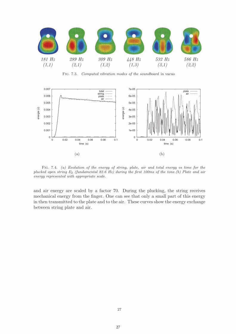
7.2. Results. We present here a couple of numerical results: eigenmodes ofthe soundboard in vacuo, energy curves and visualization of the unknowns just afterthe plucking. We refer the reader to a previous paper [18] in which a frequencyanalysis of the simulation results is performed in order to evaluate the transfer ofenergy through the various components of the coupled system and the effect of somestructural changes is presented which allows to analyze the vibroacoustical behaviorof the guitar in terms of structural, acoustic and structural-acoustic modes.
7.2.1. First eigenmodes of the soundboard in vacuo . The measurementof the eigenfrequencies and eigenmodes of the soundboard of a guitar has been thesubject of an important number of experiments [30, 41, 35]. In the present study, thepurpose was not to simulate a particular instrument. Nevertheless it is possible tocompare at least qualitatively the shape and frequencies of the simulated soundboardto existing results. Figure 7.2 shows the first 5 modes of a classical guitar soundboardclamped on its outer boundary and without cavity, observed by Jansson and Fig. 7.3shows the first six modes computed using the second order space approximation.One can see that the computed modes are in good agreement with the experiments,both for the shape and the frequencies estimations. The addition of an extra modecomparing to the real guitar is certainly due to a rather simple strutting modeling ofthe simulated soundboard.
185 Hz 287 Hz 460 Hz 508 Hz 645 Hz(1,1) (2,1) (1,2) (1,3) (2,2)
Fig. 7.2. Vibration modes of a classical guitar top plate glued to fixed ribs and without back(Jansson, 1971 [30])
7.2.2. Energy. Figure Fig. 7.4 shows the evolution of the energy during 100 mswhen plucking the lowest string of the guitar. The energy of the complete systemand the energy of the substructures of the instrument (string, plate and air) arerepresented. Since the string remains the essential part of the total energy, the plate
26
181 Hz(1,1)
289 Hz(2,1)
309 Hz(1,2)
448 Hz(1,3)
532 Hz(3,1)
586 Hz(2,2)
Fig. 7.3. Computed vibration modes of the soundboard in vacuo
0
0.001
0.002
0.003
0.004
0.005
0.006
0.007
0 0.02 0.04 0.06 0.08 0.1
ener
gie
(J)
time (s)
totalstringplate
air
(a)
0
1e-05
2e-05
3e-05
4e-05
5e-05
6e-05
7e-05
0 0.02 0.04 0.06 0.08 0.1
ener
gie
(J)
time (s)
plateair
(b)
Fig. 7.4. (a) Evolution of the energy of string, plate, air and total energy vs time for theplucked open string E2 (fundamental 82.6 Hz) during the first 100ms of the tone.(b) Plate and airenergy represented with appropriate scale.
and air energy are scaled by a factor 70. During the plucking, the string receivesmechanical energy from the finger. One can see that only a small part of this energyin then transmitted to the plate and to the air. These curves show the energy exchangebetween string plate and air.
27
27

-0.003
-0.002
-0.001
0
0.001
0.002
0.003
-0.003
-0.002
-0.001
0
0.001
0.002
0.003
-0.003
-0.002
-0.001
0
0.001
0.002
0.003
-0.003
-0.002
-0.001
0
0.001
0.002
0.003
-0.003
-0.002
-0.001
0
0.001
0.002
0.003
-0.003
-0.002
-0.001
0
0.001
0.002
0.003
Displacement of the string us ( m )
Displacement of the soundboard up ( mm )
Pressure jump at the surface of the guitar ( Pa )
Pressure in 3 orthogonal planes ( Pa )
Fig. 7.5. String displacement, plate displacement, pressure jump and pressure in 3 orthogonalplanes immediately after the plucking of the open lowest string (E6, fundamental 82.5 Hz).
7.2.3. Visualization of the unknowns. Figure 7.5 shows the evolution of thesolution immediately after the plucking of the string, that is at the very beginning ofthe free vibrations. The following quantities are represented:
• the string displacement,• the plate displacement,• the pressure jump λh at the surface of the guitar,• the pressure p in 3 orthogonal planes simultaneously, which intersect in the
middle of the cavity, under the hole.The time duration between two pictures is 0.36ms. The time evolution of the quan-tities is obviously better seen with animated pictures [6]. The pictures of plate dis-placement and of the pressure jump have been realized with the software Medit [24].Note that the pressure in the cavity is largely greater than the pressure outside. Thepressure across the surface presents thus important variations near the hole, sincethe pressure is obviously continuous across the hole. The amplitude of the string isapproximately 2mm and the amplitude of the soundboard is only of the order of 20μm.
8. Conclusion. We have presented a relatively exhaustive numerical modeling ofthe acoustic guitar. Up to our knowledge, this is the first modeling of this instrumentwhich involves the whole vibroacoustical behavior from the initial pluck to the 3Dacoustic radiation. Among other things, this numerical method can be used as atool for the estimation of quantities that are hard to measure experimentally as forexample the estimation of the relative structural losses and radiation losses in thesounds generated by the guitar [18]. It can also be seen from Fig. 7.5 that the
28

simulation results can be used for the analysis of the directivity properties of theinstrument.
This work has been made possible with the help of recent research developedin numerical methods. It must be pointed out that the complex geometry of theinstrument for the fluid-structure interaction part of the problem is taken into accountin a very efficient way via the fictitious domain method. Also, the problem is limited toa bounded cube with the help of high order absorbing boundary conditions. The mostinteresting aspect of this study is certainly the stability analysis which is based onenergy estimation derived from the numerical scheme. This efficient technique permitsto show the stability in the rather complicated case where different time-discretizationare used, namely an analytical one and a finite differences one. Furthermore, for theparticular scheme presented here, the stability conditions are optimal in the sensethat they are the same than the ones obtained for uncoupled schemes.
REFERENCES
[1] J. Argyris, I. Fried, and D. Sharpf, The TUBA family of plate elements for thematrixdisplacement method, The Aeronaultical Journal of the Royal Aeronautical Society, 72(1968), pp. 701–709.
[2] G. P. Astrakhantsev, Method of fictitious domain method for a second-order elliptic equa-tion with natural boundary conditions, USRR Compu. Math. and Math. Phys., 18 (1978),pp. 114–121.
[3] I. Babuska, The Finite Element Method with Lagrangian Multipliers, Numer. Math., 20 (1973),pp. 179–192.
[4] A. Bamberger, G. Chavent, and P. Lailly, Etude de schemas numeriques pour les equationsde l’ elastodynamique lineaire, Tech. Report 41, INRIA, 1980. Rapport Interne.
[5] J. Batoz, K. Bathe, and L. . Ho, A study of three-node triangular plate bending elements,International Journal for Numerical Methods in Enginerering, 15(2) (1980).
[6] E. Becache, A. Chaigne, G. Derveaux, and P. Joly, Numerical simulation ofthe acoustic guitar. DVD, VHS and RealPlayer document, English, March 2003.http://www.inria.fr/multimedia/Videotheque-fra.html.
[7] E. Becache, P. Joly, and C. Tsogka, Fictitious domains, mixed finite elements and perfectlymatched layers for 2d elastic wave propagation, J. Comp. Acous., 9 (2001), pp. 1175–1203.
[8] F. Brezzi and M. Fortin, Numerical approximation of mindlin-reissner plates, Mathematicsof computation, 47(175) (1986), pp. 151–158.
[9] A. Chaigne, On the use of finite differences for musical synthesis. Application to plucked stringinstruments , J. Acoust., 5 (1992), pp. 181–211.
[10] A. Chaigne and C. Lambourg, Time-domain simulation of damped impacted plates. Part I.Theory and experiments, J. Acoust. Soc. Am., 109 (2001), pp. 1422–1432.
[11] D. Chapelle, Une formulation mixte de plaque ou l’effort tranchant est approche dans sonespace naturel, tech. report, INRIA, 1993.
[12] P. Ciarlet, The finite element method for elliptic problems, North Holland, eds, 1978.[13] P. G. Ciarlet, Mathematical elasticity. Vol. II, North-Holland Publishing Co., Amsterdam,
1997. Theory of plates.[14] G. Cohen, Higher-Order Numerical Methods for Transient Wave Equations, Springer, 2002.[15] G. Cohen, P. Joly, J. E. Roberts, and N. Tordjman, Higher order triangular finite elements
with mass lumping for the wave equation, SIAM J. Numer. Anal., 38 (2001), pp. 2047–2078(electronic).
[16] F. Collino, Conditions absorbantes d’ordre eleve pour des modeles de propagation d’onde dansdes domaines rectangulaires, Tech. Report 1790, INRIA, Novembre 1992.
[17] G. Derveaux, Modelisation numerique de la guitare acoustique , PhD thesis, Ecole Polytech-nique, 2002.
[18] G. Derveaux, A. Chaigne, P. Joly, and E. Becache, Time-domain simulation of a guitar: model and method , J. Acoust. Soc. Am., 114 (2003), pp. 3368 – 3383.
[19] P. Destuynder and T. Nevers, A new finite element for bending plates, Computer Methodsin Applied Mechanics and Engineering, 68 (1988).
[20] P. Destuynder and M. Salaun, Mathematical analysis of thin plate models, vol. 24 ofMathematiques & Applications (Berlin) [Mathematics & Applications], Springer-Verlag,
29

Berlin, 1996.[21] B. Engquist and A. Majda, Absorbing boundary conditions for the numerical simulation of
waves, Math. Comp., 31 (1977), pp. 629–651.[22] P. C. et P.A. Raviart, A mixed finite element method for the biharmonic equation, in Math-
ematical Aspects of Finite Elements in Partial Differential Equations, C. de Boor, ed.,Academic Press, 1974, pp. 125–145.
[23] N. H. Fletcher and T. D. Rossing, The physics of musical instruments, Springer-Verlag,New York, second ed., 1998.
[24] P. J. Frey, Medit: An interactive mesh visualization software. www.http://www-rocq1.inria.fr/gamma/medit/.
[25] V. Girault and R. Glowinski, Error analysis of a fictitious domain method applied to aDirichlet problem, Japan J. Indust. Appl. Math., 12 (1995), pp. 487–514.
[26] R. Glowinski, Approximations externes,par elements finis de lagrange d’ordre un et deux,du probleme de dirichlet pour l’operateur biharmonique. methodes iteratives de resolutiondes problemes approches., in Topics in Numerical Analysis, J. Miller, ed., Academic Press,1973, pp. 123–171.
[27] R. Glowinski, T. Pan, and J. Periaux, A fictitious domain method for external incompress-ible viscous flow modeled by Navier-Stokes equations, Comp. Meth. in Appl. Mech. andEng., 112 (1994), pp. 133–148.
[28] R. Glowinski, T. Pan, and J. Periaux, A fictitious domain method for dirichlet problem andapplications, Comp. Meth. in Appl. Mech. and Engin., 111 (1994), pp. 283–304.
[29] T. Hughes, The finite element method: Linear static and dynamic finite element analysis,Prentice-Hall, 1987.
[30] E. Jannson, A study of acoustical and hologram interferometric measurements on the top platevibrations of of a guitar , Acustica, 25 (1971).
[31] P. Joly and L. Rhaouti, Domaines fictifs, elements finis H(div) et condition de Neumann: leprobleme de la condition inf-sup, C. R. Acad. Sci. Paris Ser. I Math., 328 (1999), pp. 1225–1230.
[32] Y. A. Kuznetsov, Fictitious component and domain decomposition methods for the solutionof eigenvalue problems, in Computing methods in applied sciences and engineering, VII(Versailles, 1985), North-Holland, Amsterdam, 1986, pp. 155–172.
[33] A. W. Leissa, Vibrations of plates, NASA SP, 160 (1969).[34] F. Millot, F. Collino, and P. Joly, Fictitious domain method for unsteady problems: ap-
plication to electromagnetic scattering, in Mathematical and numerical aspects of wavepropagation (Mandelieu-La Napoule, 1995), SIAM, Philadelphia, PA, 1995, pp. 260–269.
[35] C. S. M.J. Elejabarrieta, A. Ezcurra, Evolution of the vibrational behavior of a guitarsounboard along successive construction phases by means of the modal analysis technique, J. Acoust. Soc. Am., 108 (2000), pp. 369–378.
[36] J. Pitkaranta, Boundary Subspaces for the Finite Element Method With Lagrange Multipliers,Numer. Math., 33 (1979), pp. 273–289.
[37] L. Rhaouti, A. Chaigne, and P. Joly, Time-domain simulation and numerical modeling ofthe kettledrum , J. Acoust. Soc. Am., 105 (1999), pp. 3545 – 3562.
[38] B. Richardson and G. Roberts, The adjustment of mode frequencies in guitars: A studyby means of holographic interferometry and finite element analysis, in SMAC 83, vol. 2,Stockholm, Sweden, July 1983, pp. 285–302.
[39] B. E. Richardson, The influence of strutting of the top-plate of a guitar, Catgut AcousticalSoc. Newsletter, 40 (1983), pp. 13–17.
[40] B. E. Richardson, The acoustical development of the guitar , Catgut Acoust. Soc. J., 2(1994), pp. 181–211.
[41] T. D. Rossing and G. Eban, Normal modes of a radially braced guitar determined by TVholography, J. Acoust. Soc. Am., 106 (1999), pp. 2991–2996.
[42] K. Yosida, Functional Analysis, Springer, 1965.
30