numerical simulation of population distribution in china · of numerical grid generation has...
TRANSCRIPT
Numerical Simulation of PopulationDistribution in China
T. X. YueY. A. WangS. P. ChenJ. Y. LiuD. S. QiuX. Z. DengM. L. LiuY. Z. Tian
Chinese Academy of Sciences
A model for simulating population distribution (MSPD) of China is developed basedon the grid generation method and the Control of MapObjects of geographical in-formation system. Elevation, net primary productivity, land use and land cover, citysizes and their spatial distribution, and spatial distribution of transport infrastruc-tures are taken into full account in the MSPD. The result from the MSPD shows thatin 2000, 90.8% of the total population of China distributed on the southeastern sideof the Heihe-Tengchong line. The ratio of population on the northwestern side tototal population of China has been increasing since 1935. The yearly growth ratewas 0.8% from 1935 to 1990 and 6.1% from 1990 to 2000. One important advan-tage of the MSPD is that when scenarios of land cover, spatial distributions of trans-port infrastructures and cities are available, scenarios of spatial population distribu-tion can be developed on the basis of total population forecast.
KEY WORDS: population distribution; numerical simulation; grid generation; geographicalinformation system.
Please address correspondence to T. X. Yue, Institute of Geographical Sciences and Natu-ral Resources Research, Chinese Academy of Sciences, 917 Building, Datun, Anwai, 100101Beijing, P. R. China; e-mail: [email protected].
Population and Environment, Vol. 25, No. 2, November 2003 2003 Human Sciences Press, Inc. 141
142
POPULATION AND ENVIRONMENT
INTRODUCTION
The analysis of human population distribution represents a particularlyinfluential line of enquiry (Woods & Rees, 1986). It traces back to the statis-tical revolution that began in Europe and America in the 19th century andresulted from the combination of regular population censuses with vitalregistration data organized and manipulated within a framework of admin-istrative units (Cullen, 1975; Cassedy, 1984). Approaches to estimating pop-ulation distribution within administrative units can be divided into two cat-egories that are areal interpolation and surface Modelling (Deichmann,1996).
Areal interpolation is the transformation of data between different setsof areal units (Goodchild & Lam, 1980). The set of zones, for which dataare available, is termed source zones. The second set of zones, for whichestimates need to be derived, is termed target zones. The third set of zones,for which auxiliary information can be incorporated in the interpolationprocess, is termed control zones (Goolchild et al., 1993; Moxey & Allan-son, 1994). The methods of areal interpolation based on alternative hypoth-eses include radially symmetric kernel functions (Parr, 1985; Bracken &Martin, 1989), maximally smooth estimation (Tobler, 1979), piecewise ap-proximation (Flowerdew et al., 1991), uniform target-zone densities (Good-child & Lam, 1980), and uniform control-zone densities (Flowerdew &Green, 1989).
Surface Modelling is aimed at formulating population in a regular gridsystem, in which each grid contains an estimate of total population that isrepresentative for that particular location. Representing data in grid formhas at least three advantages: (1) regular grid can be easily re-aggregatedto any areal arrangement required; (2) producing population data in gridform is one way of ensuring compatibility between heterogeneous data sets;and (3) converting data into grid form can provide a way of avoiding someof the problems imposed by artificial political boundaries (Martin & Bracken,1991; Deichmann, 1996). Compiling population data in grid form is by nomeans a new approach. For instance, Adams (1968) presented a computergenerated grid map of population density in West Africa; Population Atlasof China presented grid population data for several regions in China (Insti-tute of Geography of Chinese Academy of Sciences, 1987).
The surface Modelling consists of three basic steps: (1) a surface ofweighting factors is created in a regular grid system for the study areas; (2)the basic weights derived in the first step are adjusted by using auxiliarydata sources, and (3) total population in the study areas is distributed to thecorresponding grids in proportion to the weights constructed in the previ-
143
T. X. YUE ET AL.
ous steps. In this paper, a model for simulating population distribution isdeveloped on the basis of an improvement on surface modelling by intro-ducing grid generation method.
METHODS
The Model for Simulating Population Distribution (MSPD)
Sir Isaac Newton propounded his Law of Universal Gravitation in 1687,i.e., any two bodies attract each other in proportion to the product of theirmasses and in inverse proportion to the square of their distance. In analogyto physical gravity model, the concept of potential population distributionwas developed, which is a measure of average accessibility of a given loca-tion with respect to the size and location of other features (Plane & Roger-son, 1994; Deichmann, 1996). The influence of a city upon a grid is as-sumed to be proportional to the city’s size, weighted inversely by thedistance of separation between the grid and the city. Within a given thresh-old distance, the potential population distribution is formulated as (1)
Pij = ∑M
k=1
Sk(dijk )
a(1)
where pij is the population at grid (i, j); Sk is the size of city k; dijk is thedistance between grid (i, j) and city k; M is the total number of cities withinthe given threshold distance; and a is exponent to be simulated.
In fact, spatial distribution of population is greatly influenced by natu-ral factors, especially net primary productivity (NPP) and elevation. Theinfluence of each of these factors is not simple. It depends on economicfactors such as spatial distribution of transport infrastructures and cities. Forinstance, when a railway traverses Qinghai-Xizang plateau of China, or whena new city appears, the distribution of population is immediately modified.The growth of means of transport is fundamental in distribution of popula-tion. In China, an increasing contrast becomes manifest between regions al-ready reached by modern and those not so affected. The former developsrapidly, in which great cities expanded at an accelerating pace. Transportfavors the growth of cities. Cities are one of the major elements in thedistribution of population. In general it is possible to distinguish a centraland more densely peopled nucleus and a peripheral residential area andextended star-like along the lines of transportation. The influence of citieson the distribution of population is exercised directly through the concen-
144
POPULATION AND ENVIRONMENT
tration of people and also indirectly through the swarms of suburbanitesscattered over their peripheral countryside in dormitory suburbs or satellitetowns.
Therefore, in addition to the size of city k and the distance betweengrid (i, j) and city k embodied in the formulation (1), land cover, net primaryproductivity, transport infrastructures and elevation are involved in theMSPD. The MSPD introduced in this paper is generally formulated as,
MSPDij (t) = G(n,t) � Wij(t) � f1 (Tranij(t)) � f2 (NPPij(t)) � f3 (DEMij)) (2)� f4(uij(t))
where t is the time variable; G(n,t) is a parameter determined by total popu-lation in administrative division n where grid (i, j) is located; Wij(t) is anindicative factor of water area; f1(Tranij) is a function determined by thecondition of transport infrastructures of grid (i, j); f2(NPPij) is a function de-termined by the condition of net primary productivity of grid (i, j); f3(DEMij)is a function determined by the elevation of grid (i, j); f4(uij(t)) is a functiondetermined by contribution of urban areas to population density at grid (i,
j); uij(t ) = ∑M(t)
k=1
(Sk (t ))a1
(dijk(t ))a2, Sk(t) is size of the kth city, M(t) is the total number of
cities, dijk is the distance from grid (i, j) to the core grid of the kth city, a1
and a2 are exponents to be simulated.
Grid Generation
In 1960s, grid generation techniques began to be developed (Morrison,1962; Sidorov, 1966; Ahuja & Coons, 1968). The successful developmentof numerical grid generation has already formed a separate mathematicaldiscipline. In the 1990s, grid techniques reached a new stage. The uniqueaspect of grid generation on general domain is that grid generation is notobliged to have any specified formulation and any foundation may be suit-able for the purpose if the grid generated is acceptable. The most importantstep is to find an appropriate transformation between computational do-main and physical domain for purposes (Liseikin, 1999).
A number of grid generation methods have been developed and everyone of them has its strengths and weaknesses. This paper chooses the mostefficient method, which is based on the gravity model, for the specific issueof population distribution of China, taking net primary productivity, eleva-tion, city sizes and their spatial distribution, spatial distribution of transportinfrastructures and grid location into full account.
145
T. X. YUE ET AL.
MATERIALS AND DATA ACQUISITION
Spatial Distribution of Cities in China
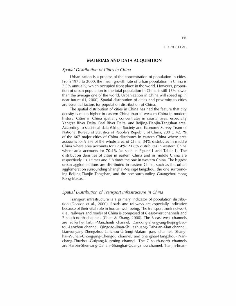
Urbanization is a process of the concentration of population in cities.From 1978 to 2000, the mean growth rate of urban population in China is7.5% annually, which occupied front place in the world. However, propor-tion of urban population to the total population in China is still 15% lowerthan the average one of the world. Urbanization in China will speed up innear future (Li, 2000). Spatial distribution of cities and proximity to citiesare essential factors for population distribution of China.
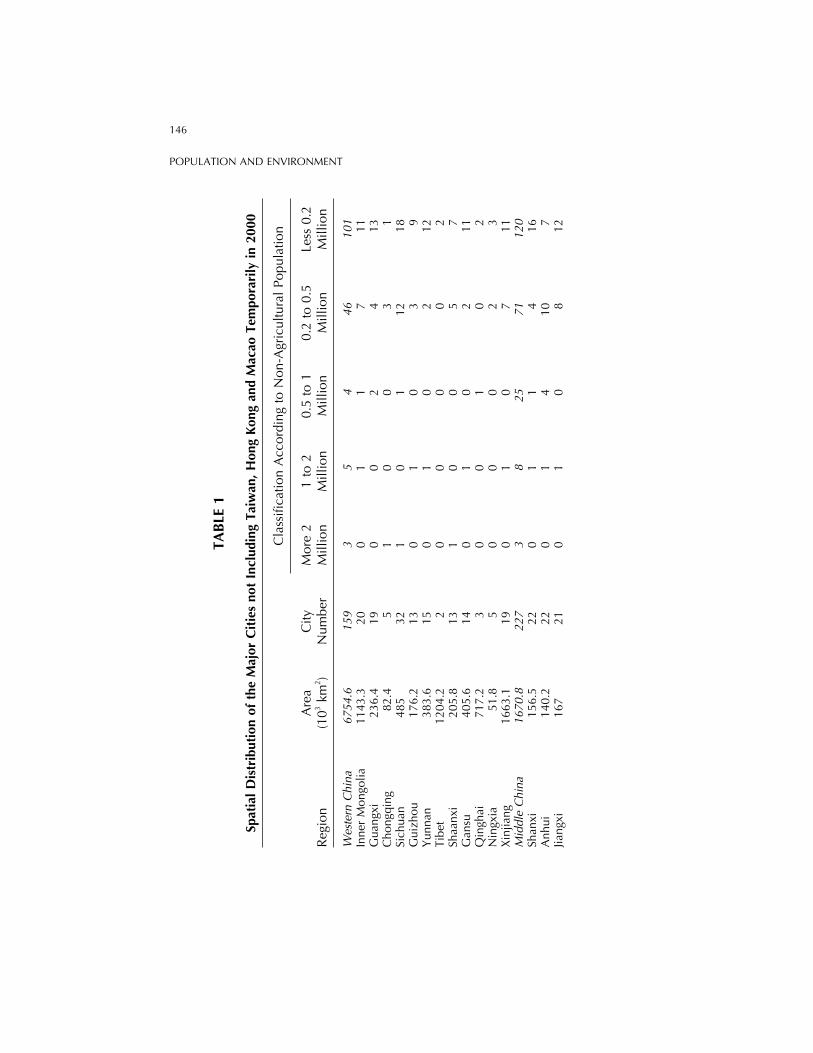
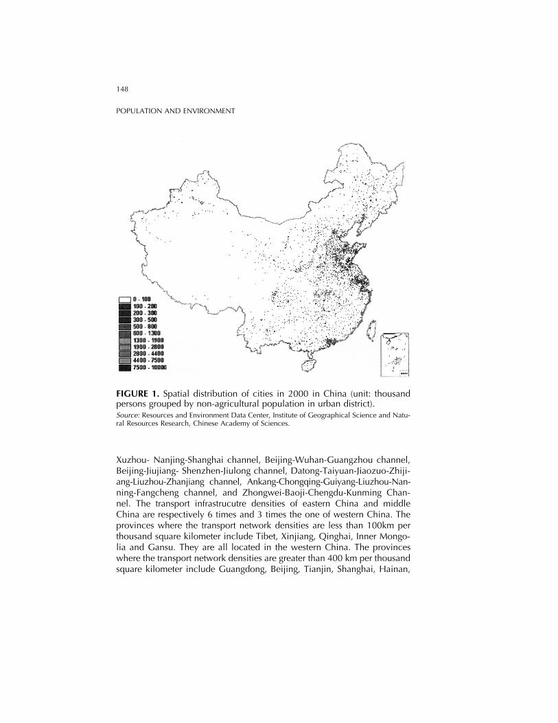
The spatial distribution of cities in China has had the feature that citydensity is much higher in eastern China than in western China in modernhistory. Cities in China spatially concentrates in coastal area, especiallyYangtze River Delta, Peal River Delta, and Beijing-Tianjin-Tangshan area.According to statistical data (Urban Society and Economy Survey Team ofNational Bureau of Statistics of People’s Republic of China, 2001), 42.1%of the 667 major cities of China distributes in eastern China where areaaccounts for 9.5% of the whole area of China; 34% distributes in middleChina where area accounts for 17.4%; 23.8% distributes in western Chinawhere area accounts for 70.4% (as seen in Figure 1 and Table 1). Thedistribution densities of cities in eastern China and in middle China arerespectively 13.1 times and 5.8 times the one in western China. The biggesturban agglomerations are distributed in eastern China, such as the urbanagglomeration surrounding Shanghai-Najing-Hangzhou, the one surround-ing Beijing-Tianjin-Tangshan, and the one surrounding Guangzhou-HongKong-Macao.
Spatial Distribution of Transport Infrastructure in China
Transport infrastructure is a primary indicator of population distribu-tion (Dobson et al., 2000). Roads and railways are especially indicativebecause of their vital role in human well-being. The transport trunk network(i.e., railways and roads) of China is composed of 6 east-west channels and7 south-north channels (Chen & Zhang, 2000). The 6 east-west channelsare Suifenhe-Harbin-Manzhouli channel, Dandong-Shengyang-Beijing-Bao-tou-Lanzhou channel, Qingdao-Jinan-Shijiazhuang- Taiyuan-Xian channel,Lianyungang-Zhengzhou-Lanzhou-Urumqi-Alatam pass channel, Shang-hai-Wuhan-Chongqing-Chengdu channel, and Shanghai-Hangzhou- Nan-chang-Zhuzhou-Guiyang-Kunming channel. The 7 south-north channelsare Harbin-Shenyang-Dalian–Shanghai-Guangzhou channel, Tianjin-Jinan-
146
POPULATION AND ENVIRONMENT
TABLE1
SpatialDistributionoftheMajorCitiesnotIncludingTaiwan,HongKongandMacaoTemporarilyin2000
Cla
ssifi
catio
nA
ccor
ding
toN
on-A
gric
ultu
ral
Popu
latio
n
Are
aC
ityM
ore
21
to2
0.5
to1
0.2
to0.
5Le
ss0.
2R
egio
n(1
03km
2 )N
umbe
rM
illio
nM
illio
nM
illio
nM
illio
nM
illio
n
WesternChina
6754.6
159
35
446
101
Inne
rM
ongo
lia11
43.3
200
11
711
Gua
ngxi
236.
419
00
24
13C
hong
qing
82.4
51
00
31
Sich
uan
485
321
01
1218
Gui
zhou
176.
213
01
03
9Y
unna
n38
3.6
150
10
212
Tibe
t12
04.2
20
00
02
Shaa
nxi
205.
813
10
05
7G
ansu
405.
614
01
02
11Q
ingh
ai71
7.2
30
01
02
Nin
gxia
51.8
50
00
23
Xin
jiang
1663
.119
01
07
11MiddleChina
1670.8
227
38
2571
120
Shan
xi15
6.5
220
11
416
Anh
ui14
0.2
220
14
107
Jiang
xi16
721
01
08
12

147
T. X. YUE ET AL.
Hen
an16
5.7
380
27
821
Hub
ei18
636
10
412
19H
unan
211.
829
01
38
17Jil
in18
9.2
281
10
1115
Hel
ongj
iang
454.
431
11
610
13EasternChina
912.71
276
714
23100
132
Bei
jing
16.4
11
00
00
Tian
jin11
.81
10
00
0H
ebei
188.
334
03
35
23Li
aoni
ng14
6.8
312
26
714
Shan
ghai
7.6
11
00
00
Jiang
su10
541
13
323
11Z
hejia
ng10
535
01
27
25Fu
jian
122.
323
01
14
17Sh
ando
ng15
7.8
480
36
2316
Gua
ngdo
ng17
.79
521
12
2919
Hai
nan
33.9
29
00
02
7
Source:
Nat
iona
lB
urea
uof
Stat
istic
s,20
01.
148
POPULATION AND ENVIRONMENT
FIGURE 1. Spatial distribution of cities in 2000 in China (unit: thousandpersons grouped by non-agricultural population in urban district).Source: Resources and Environment Data Center, Institute of Geographical Science and Natu-ral Resources Research, Chinese Academy of Sciences.
Xuzhou- Nanjing-Shanghai channel, Beijing-Wuhan-Guangzhou channel,Beijing-Jiujiang- Shenzhen-Jiulong channel, Datong-Taiyuan-Jiaozuo-Zhiji-ang-Liuzhou-Zhanjiang channel, Ankang-Chongqing-Guiyang-Liuzhou-Nan-ning-Fangcheng channel, and Zhongwei-Baoji-Chengdu-Kunming Chan-nel. The transport infrastrucutre densities of eastern China and middleChina are respectively 6 times and 3 times the one of western China. Theprovinces where the transport network densities are less than 100km perthousand square kilometer include Tibet, Xinjiang, Qinghai, Inner Mongo-lia and Gansu. They are all located in the western China. The provinceswhere the transport network densities are greater than 400 km per thousandsquare kilometer include Guangdong, Beijing, Tianjin, Shanghai, Hainan,
149
T. X. YUE ET AL.
Shandong and Fujian (National Bureau of Statistics of People’s Republic ofChina, 2001). They are all distributed in the eastern China. The averagetransport situation in China is that from northwest to southeast the transportnetwork density becomes greater and greater (as seen in Table 2, Figure 2and Figure 3).
Land Cover and Spatial Distribution of NPP in China
Land cover is a good indicator of spatial population distribution. Inmost regions, population would range from extremely low density in desert,water, wetlands, ice, or tundra land cover to high density in developed landcover associated urban land cover, between which arid grasslands, forests,and cultivated lands would range (Dobson et al., 2000). The land coverdatabase of China in 2000 is derived from Landsat Thematic Mapper (TM)imagery at 30-m resolution (Figure 4)
Net primary productivity (NPP) is the difference between accumulativephotosynthesis and accumulative autotrophic respiration by green plantsper unit time and space (Lieth and Whittaker, 1975). The Boreal EcosystemsProductivity Simulator (Liu et al., 1997) is employed for analyzing spatialdistribution of NPP in China. It integrates different data types that includeNOAA/AVHRR data at 1-km resolution in lambert conformal conic projec-tion, daily meteorological data in Gaussian grided systems, and soil datagrouped in polygons.
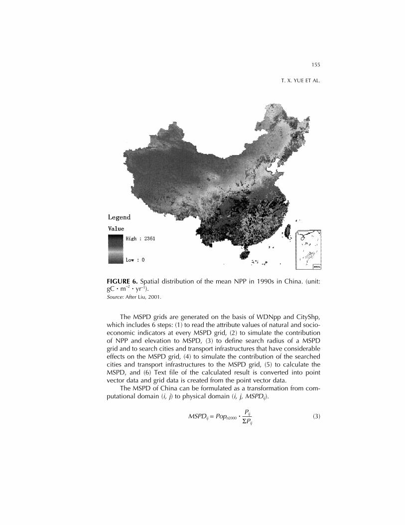
The general situation in China is that from southeast to northwest NPPbecomes smaller and smaller gradually. Most of the NPP is distributed inthe East of the rainfall line where the annual precipitation is 410 mm (asseen in Figure 5 and Figure 6), excepting that there is higher NPP in thesouthern slopes of Tianshan mountains and Altai mountains in Xinjiang.The maximum NPP appears in Xiaoxinganling mountain and Changbaimountain in the northeast China, Yunnan-Guizhou plateau, Guangxi, Hai-nan, Chongqin and provinces along middle and lower reaches of Yangtzeriver.
In terms of land cover types, on the average (as seen in Table 3), NPPof shrub and open forest is 1071 gC � m−2 � yr−1, evergreen broad-leavedforest 975 gC � m−2 � yr−1, deciduous broad-leaved forest 928 gC � m−2 � yr−1,coniferous and broad-leaved mixed forest 870 gC � m−2 � yr−1, farmland sys-tem 752 gC � m−2 � yr−1, evergreen coniferous forest 587 gC � m−2 � yr−1, de-ciduous coniferous forest 585 gC � m−2 � yr−1, and grassland 271 gC � m−2 �yr−1 (Liu, 2001).

150
POPULATION AND ENVIRONMENT
TABLE 2
Spatial Distribution of Rail and Road not Including Taiwan,Hong Kong and Macao Temporarily in 2000
Railway + Road Railway RoadRegion (km/103 km2) (km/103 km2) (km/103 km2)
Western China 86 4 82Inner Mongolia 64 5 59Guangxi 234 10 224Chongqing 362 7 355Sichuan 193 5 187Guizhou 206 10 197Yunnan 291 5 286Tibet 19 0 19Shaanxi 227 13 214Gansu 105 8 97Qinghai 28 2 26Ningxia 212 16 196Xinjiang 23 2 21Middle China 262 19 243Shanxi 379 25 354Anhui 338 21 317Jiangxi 243 21 222Henan 417 28 389Hubei 328 17 311Hunan 304 17 287Jilin 206 20 186Helongjiang 125 15 111Eastern China 511 26 486Beijing 940 111 829Tianjin 840 82 758Hebei 346 32 314Liaoning 345 34 310Shanghai 621 52 569Jiangsu 282 14 269Zhejiang 408 12 396Fujian 425 7 418Shandong 473 25 448Guangdong 5845 78 5768Hainan 520 7 513
Source: National Bureau of Statistics, 2001.

151
T. X. YUE ET AL.
FIGURE 2. Spatial distribution of roads in 2000 in China.Source: Resources and Environment Data Center, Institute of Geographical Science and Natu-ral Resources Research, Chinese Academy of Sciences.
Elevation
Elevation is an important variable in population distribution modellingof China because most human settlements occur on lower elevation inChina. The terrestrial parts of China are broadly divided into three steps asseen in Figure 7 from Qinghai-Xizang Plateau eastward (Zhao, 1986). Thelofty and extensive Qinghai-Xizang Plateau is the first great topographicstep. Its eastern and northern borders roughly coincide with the 3000mcontour line. It generally has an elevation of 4000m to 5000m and henceis called the roof of the world.
From the eastern margin of the Qinghai-Xizang Plateau eastward up tothe Da Hinggan-Taihang-Wushan mountains lies the second great topo-graphic step. It is mainly composed of plateaus and basins with elevationsof 1000 to 2000m, such as the Nei Mongol, Ordos, Loess and Yunnan-Guizhou plateaus and the Tarim, Junggar, and Sichuan basins.
152
POPULATION AND ENVIRONMENT
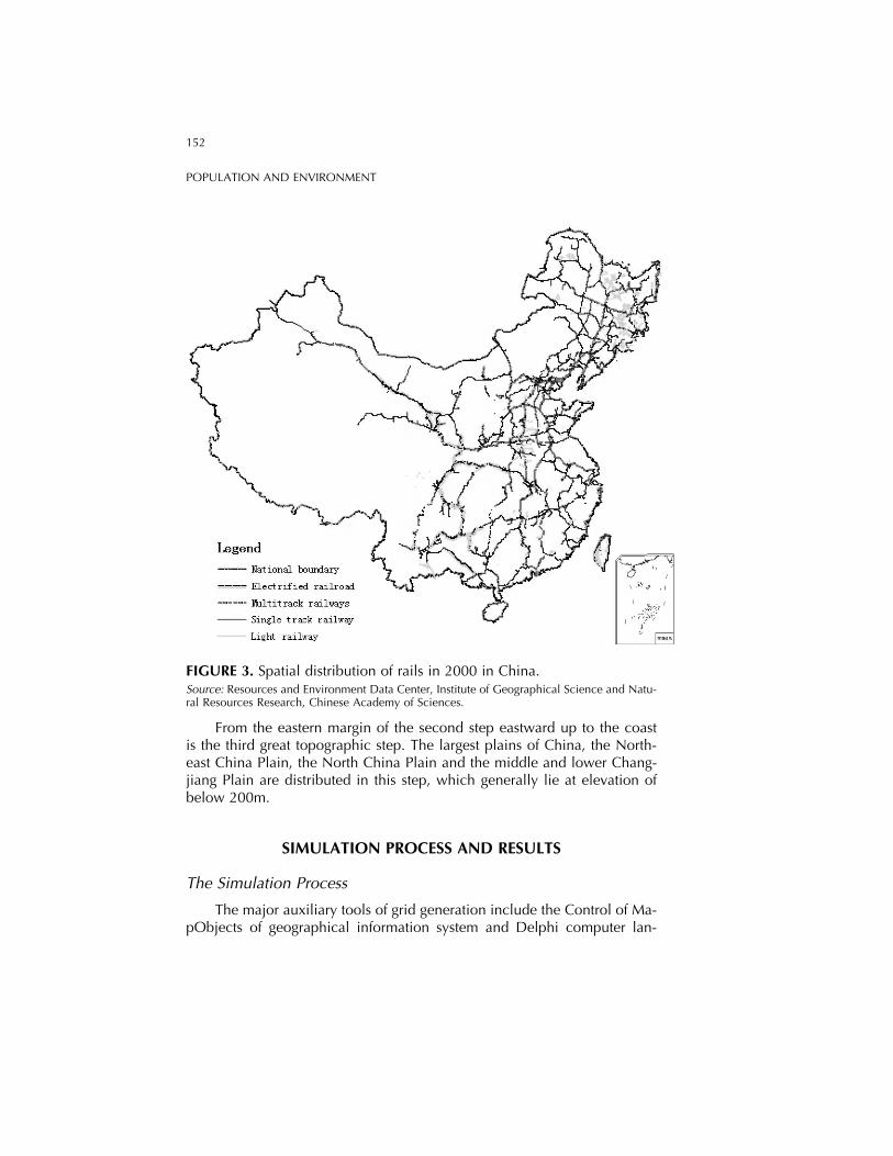
FIGURE 3. Spatial distribution of rails in 2000 in China.Source: Resources and Environment Data Center, Institute of Geographical Science and Natu-ral Resources Research, Chinese Academy of Sciences.
From the eastern margin of the second step eastward up to the coastis the third great topographic step. The largest plains of China, the North-east China Plain, the North China Plain and the middle and lower Chang-jiang Plain are distributed in this step, which generally lie at elevation ofbelow 200m.
SIMULATION PROCESS AND RESULTS
The Simulation Process
The major auxiliary tools of grid generation include the Control of Ma-pObjects of geographical information system and Delphi computer lan-

153
T. X. YUE ET AL.
TABLE 3
NPP in Terms of Land Cover Types on the Average
Land Cover type NPP (gC � m−2 � yr−1)
Shrub and open forest 1071Evergreen broad-leaved forest 975Deciduous broad-leaved forest 928Coniferous and broad-leaved mixed forest 870Farmland system 752Evergreen coniferous forest 587Deciduous coniferous forest 585Grassland 271
FIGURE 4. Land cover of China in 2000.Source: Resources and Environment Data Center, Institute of Geographical Science and Natu-ral Resources Research, Chinese Academy of Sciences.
154
POPULATION AND ENVIRONMENT
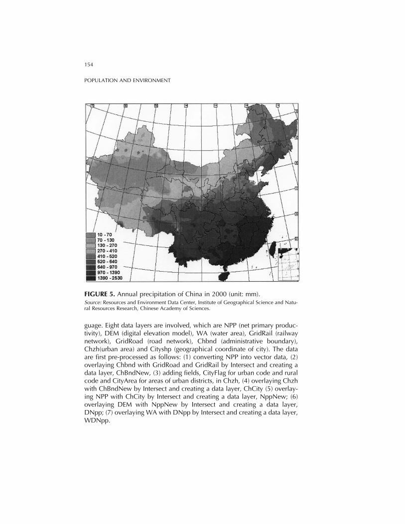
FIGURE 5. Annual precipitation of China in 2000 (unit: mm).Source: Resources and Environment Data Center, Institute of Geographical Science and Natu-ral Resources Research, Chinese Academy of Sciences.
guage. Eight data layers are involved, which are NPP (net primary produc-tivity), DEM (digital elevation model), WA (water area), GridRail (railwaynetwork), GridRoad (road network), Chbnd (administrative boundary),Chzh(urban area) and Cityshp (geographical coordinate of city). The dataare first pre-processed as follows: (1) converting NPP into vector data, (2)overlaying Chbnd with GridRoad and GridRail by Intersect and creating adata layer, ChBndNew, (3) adding fields, CityFlag for urban code and ruralcode and CityArea for areas of urban districts, in Chzh, (4) overlaying Chzhwith ChBndNew by Intersect and creating a data layer, ChCity (5) overlay-ing NPP with ChCity by Intersect and creating a data layer, NppNew; (6)overlaying DEM with NppNew by Intersect and creating a data layer,DNpp; (7) overlaying WA with DNpp by Intersect and creating a data layer,WDNpp.
155
T. X. YUE ET AL.
FIGURE 6. Spatial distribution of the mean NPP in 1990s in China. (unit:gC � m−2 � yr−1).Source: After Liu, 2001.
The MSPD grids are generated on the basis of WDNpp and CityShp,which includes 6 steps: (1) to read the attribute values of natural and socio-economic indicators at every MSPD grid, (2) to simulate the contributionof NPP and elevation to MSPD, (3) to define search radius of a MSPDgrid and to search cities and transport infrastructures that have considerableeffects on the MSPD grid, (4) to simulate the contribution of the searchedcities and transport infrastructures to the MSPD grid, (5) to calculate theMSPD, and (6) Text file of the calculated result is converted into pointvector data and grid data is created from the point vector data.
The MSPD of China can be formulated as a transformation from com-putational domain (i, j) to physical domain (i, j, MSPDij).
MSPDij = Popn2000 �Pij
ΣPij(3)

156
POPULATION AND ENVIRONMENT
FIGURE 7. Digital elevation model of China (unit: m).Source: Resources and Environment Data Center, Institute of Geographical Science and Natu-ral Resources Research, Chinese Academy of Sciences.
Pij = Wij(Tranij)1.3 � (NPPij)
0.0001 � (DEMij)0.7 � (uij)
1.2 (4)
Tranij = raij + roijMaxi,j
{raij + roij}(5)
NPPij = exp� − (MNPPij − 800)2
106 � (6)
DEMij(t) = � 500(demij(t))
2demij(t) ≥ 3700m
500demij(t)
500m⟨demij(t)⟨3700m
1 demij(t) ≤ 500m
(7)

157
T. X. YUE ET AL.
uij = ∑M
k=1
Skdijk
(8)
where Popn2000 is total population in administrative division n where grid(i, j) is located; Wij is the indicative factor of water area, when grid cell(i, j) is located in water area Wij = 0, or else Wij = 1; raij and roij representrespectively rail density and road density at grid (i, j); Sk is size of the kthcity; M is the total number of cities; dijk is the distance from grid (i, j) to thecore grid of the kth city; MNPPij is the mean net primary productivity annu-ally in 1990s at grid (i, j); and demij is elevation at grid (i, j).
Results
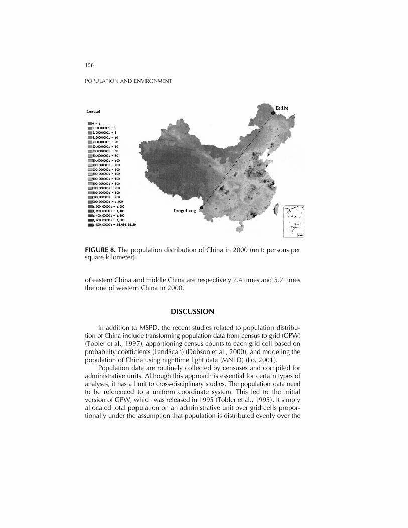
In 1935, Hu published his research results on the distribution of popu-lation in China and introduced a critical line, of which two end pointsHeihe city in Heilongjiang province and Tengchong city in Yunnan prov-ince. This Heihe-Tengchong line is located in the ecologically fragile zonewhere southeastern monsoon meets with westerlies (Chen, 2002). The ele-vation of the area on southeastern side of the Heihe-Tengchong line is378m on an average. Hu found that 96% of population in China lived inthe southeastern side of the Heihe-Tengchong line, where the area is 4.117million square kilometers accounting for 42.9% of the whole of China. In1990, the fourth census of China showed that on the southeastern side ofthe Heihe-Tengchong line there was 94.3% of the total population of Chinaand population density on the southeastern side was 22 times the one onthe northwestern side of the Heihe-Tengchong line (Zhang, 1997). The cal-culated result of MSPD shows that the southeastern side of the Heihe-Teng-chong line had 90.8% of the total population of China in 2000 (as seen inFigure 8). In other words, the ratio of population on the northwestern sideof the Heihe-Tengchong line to total population of China has been increas-ing since 1935. The growth rate was yearly 0.8% from 1935 to 1990 andyearly 6.1% from 1990 to 2000.
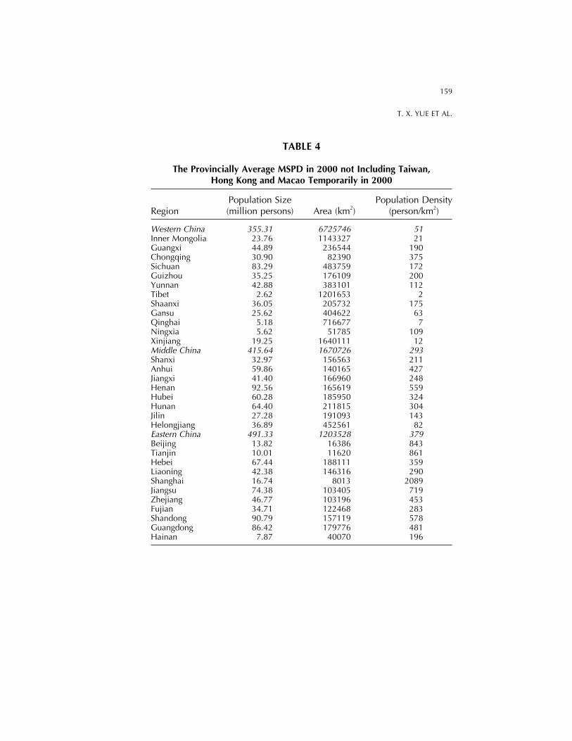
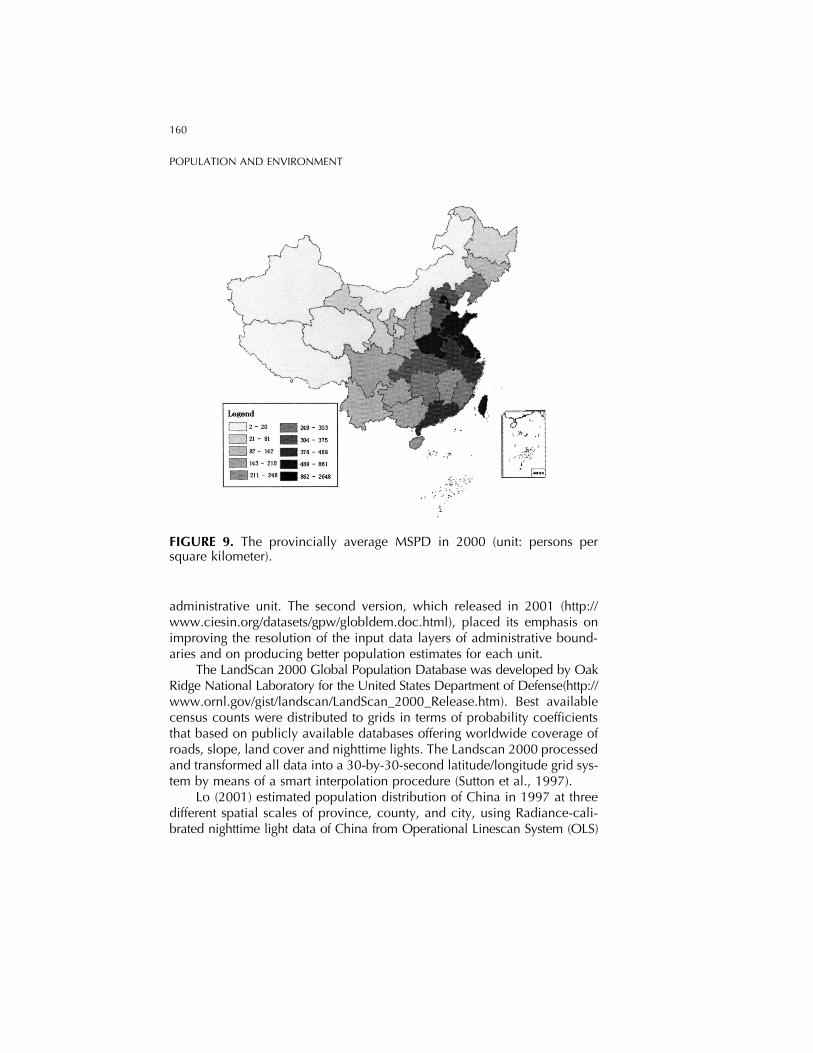
In terms of the provincially mean values, Shanghai, Tianjin and Beijinghave the highest densities that are respectively 2089, 861 and 843 personsper square kilometer in 2000. Jiangsu, Shandong and Henan have higherdensities that are respectively 719, 578 and 559 persons per square kilome-ter. The mean densities of Hunan, Hubei, Hebei, Chongqing, Anhui, Zheji-ang and Guangdong range between 304 and 481 persons per square kilo-meter. The lowest densities appear in Tibet, Qinghai, Xinjiang and InnerMongolia (as seen in Table 4 and Figure 9). In general, the average MSPD
158
POPULATION AND ENVIRONMENT
FIGURE 8. The population distribution of China in 2000 (unit: persons persquare kilometer).
of eastern China and middle China are respectively 7.4 times and 5.7 timesthe one of western China in 2000.
DISCUSSION
In addition to MSPD, the recent studies related to population distribu-tion of China include transforming population data from census to grid (GPW)(Tobler et al., 1997), apportioning census counts to each grid cell based onprobability coefficients (LandScan) (Dobson et al., 2000), and modeling thepopulation of China using nighttime light data (MNLD) (Lo, 2001).
Population data are routinely collected by censuses and compiled foradministrative units. Although this approach is essential for certain types ofanalyses, it has a limit to cross-disciplinary studies. The population data needto be referenced to a uniform coordinate system. This led to the initialversion of GPW, which was released in 1995 (Tobler et al., 1995). It simplyallocated total population on an administrative unit over grid cells propor-tionally under the assumption that population is distributed evenly over the
159
T. X. YUE ET AL.
TABLE 4
The Provincially Average MSPD in 2000 not Including Taiwan,Hong Kong and Macao Temporarily in 2000
Population Size Population DensityRegion (million persons) Area (km2) (person/km2)
Western China 355.31 6725746 51Inner Mongolia 23.76 1143327 21Guangxi 44.89 236544 190Chongqing 30.90 82390 375Sichuan 83.29 483759 172Guizhou 35.25 176109 200Yunnan 42.88 383101 112Tibet 2.62 1201653 2Shaanxi 36.05 205732 175Gansu 25.62 404622 63Qinghai 5.18 716677 7Ningxia 5.62 51785 109Xinjiang 19.25 1640111 12Middle China 415.64 1670726 293Shanxi 32.97 156563 211Anhui 59.86 140165 427Jiangxi 41.40 166960 248Henan 92.56 165619 559Hubei 60.28 185950 324Hunan 64.40 211815 304Jilin 27.28 191093 143Helongjiang 36.89 452561 82Eastern China 491.33 1203528 379Beijing 13.82 16386 843Tianjin 10.01 11620 861Hebei 67.44 188111 359Liaoning 42.38 146316 290Shanghai 16.74 8013 2089Jiangsu 74.38 103405 719Zhejiang 46.77 103196 453Fujian 34.71 122468 283Shandong 90.79 157119 578Guangdong 86.42 179776 481Hainan 7.87 40070 196
160
POPULATION AND ENVIRONMENT
FIGURE 9. The provincially average MSPD in 2000 (unit: persons persquare kilometer).
administrative unit. The second version, which released in 2001 (http://www.ciesin.org/datasets/gpw/globldem.doc.html), placed its emphasis onimproving the resolution of the input data layers of administrative bound-aries and on producing better population estimates for each unit.
The LandScan 2000 Global Population Database was developed by OakRidge National Laboratory for the United States Department of Defense(http://www.ornl.gov/gist/landscan/LandScan_2000_Release.htm). Best availablecensus counts were distributed to grids in terms of probability coefficientsthat based on publicly available databases offering worldwide coverage ofroads, slope, land cover and nighttime lights. The Landscan 2000 processedand transformed all data into a 30-by-30-second latitude/longitude grid sys-tem by means of a smart interpolation procedure (Sutton et al., 1997).
Lo (2001) estimated population distribution of China in 1997 at threedifferent spatial scales of province, county, and city, using Radiance-cali-brated nighttime light data of China from Operational Linescan System (OLS)
161
T. X. YUE ET AL.
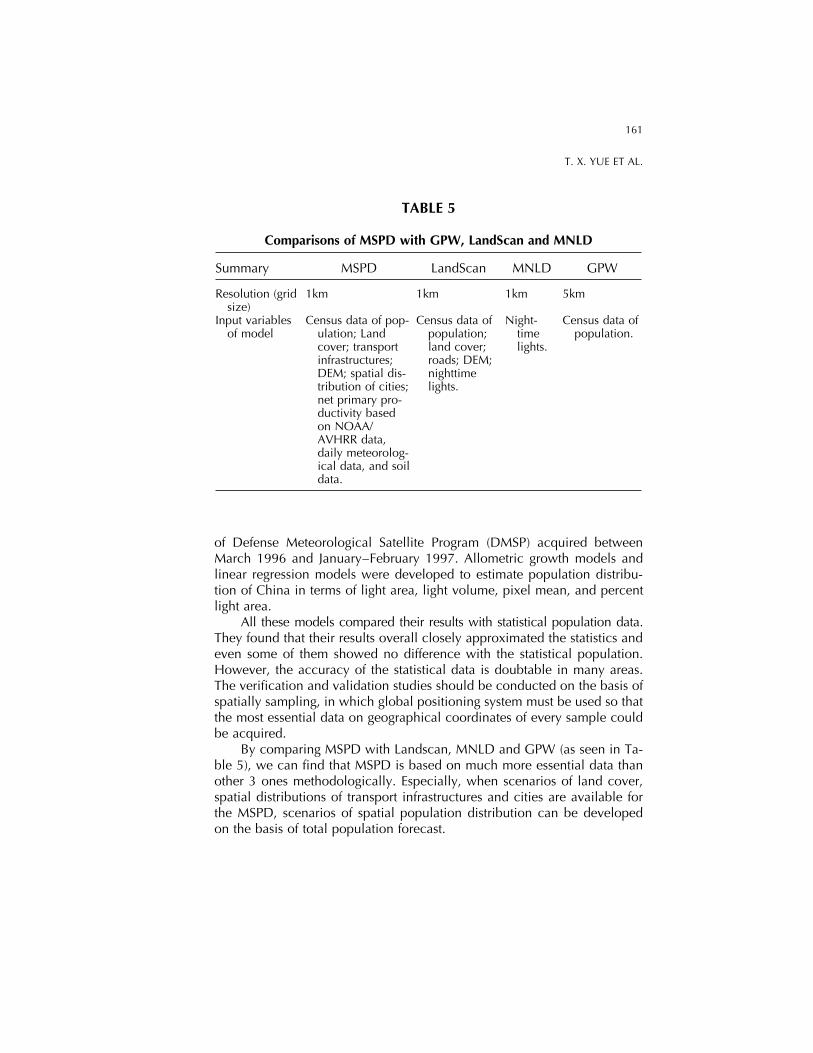
TABLE 5
Comparisons of MSPD with GPW, LandScan and MNLD
Summary MSPD LandScan MNLD GPW
Resolution (grid 1km 1km 1km 5kmsize)
Input variables Census data of pop- Census data of Night- Census data ofof model ulation; Land population; time population.
cover; transport land cover; lights.infrastructures; roads; DEM;DEM; spatial dis- nighttimetribution of cities; lights.net primary pro-ductivity basedon NOAA/AVHRR data,daily meteorolog-ical data, and soildata.
of Defense Meteorological Satellite Program (DMSP) acquired betweenMarch 1996 and January–February 1997. Allometric growth models andlinear regression models were developed to estimate population distribu-tion of China in terms of light area, light volume, pixel mean, and percentlight area.
All these models compared their results with statistical population data.They found that their results overall closely approximated the statistics andeven some of them showed no difference with the statistical population.However, the accuracy of the statistical data is doubtable in many areas.The verification and validation studies should be conducted on the basis ofspatially sampling, in which global positioning system must be used so thatthe most essential data on geographical coordinates of every sample couldbe acquired.
By comparing MSPD with Landscan, MNLD and GPW (as seen in Ta-ble 5), we can find that MSPD is based on much more essential data thanother 3 ones methodologically. Especially, when scenarios of land cover,spatial distributions of transport infrastructures and cities are available forthe MSPD, scenarios of spatial population distribution can be developedon the basis of total population forecast.
162
POPULATION AND ENVIRONMENT
ACKNOWLEDGMENT
This work is supported by Projects of National Natural Science Foun-dation of China (40371094 & 90202002), and by National Basic ResearchPriorities Program (2002CB4125) of Ministry of Science and Technology ofthe People’s Republic of China.
REFERENCES
Adams, J., (1968). A population map of West Africa, Graduate School of Geography discussionpaper No. 26. London: London School of Economics.
Ahuja, D.V., & Coons, S.A., (1968). geometry for construction and display. IBM Systems Jour-nal, 7, 188–205.
Bracken, I., & Martin, D. (1989). The generation of spatial population distribution from censuscentroid data. Environment and Planning A 21, 537–543.
Cassedy, J. H. (1984). American Medicine and Statistical Thinking, 1800–1860. Cambridge,MA: Harvard University Press.
Chen, H., & Zhang, W.C. (2000). Transport Geography of China. Beijing: Science Press (inChinese).
Chen, S. P., (2002). The spatial-temporal analysis of census. China Population, Resources andEnvironment 12(4), 3–7.
Contanza, R., d’Arge, R., de Groot, R., Farber, S., Grasso, M., Hannon, B., Limburg, K.,Naeem, S., O’Neill, R.V., Paruelo, J., Raskin, R.G., Sutton, P., & van den Belt, M. (1997).The value of the world’s ecosystem services and natural capitals. Nature, 387, 253–260.
Cullen, J. (1975). The Statistical Movement in Early Victorian Britain: the foundation of empiri-cal social science. Brighton: Hassocks.
Deichmann, U. (1996). A Review of Spatial Population Database Design and Modeling. Tech-nical Report 96-3, National Center for Geographic Information and Analysis, USA.
Dobson, J.E., Bright, E.A., Coleman, P.R., Durfee, R.C., & Worley, B.A. (2000). LandScan: aglobal population database for estimating populations at risk. Photogrammetric Engineer-ing & Remote Sensing, 66(7), 849–857.
Flowerdew, R., & Green, M. (1989). Statistical methods for inference between incompatiblezonal systems. In M.F. Goodchild & S. Gopal (Eds.), Accuracy of Spatial Database (pp.239–248). London: Taylor and Francis.
Flowerdew, R., Green, M., & Kehris, E. (1991). Using areal interpolation methods in geo-graphic information systems. Papers in Regional Science, 70, 303–315.
Goodchild, M.F., Anselin, L., & Deichmann, U. (1993). A framework for the areal interpola-tion of socioeconomic data. Environment and Planning, A 25, 383–397.
Goodchild, M.F., & Lam, N.S.N. (1980). Areal interpolation: a variant of the traditional spatialproblem. Geo-Preocessing, 1, 297–312.
Hu, H.Y. (1935). The distribution of population in ChinaLBOLE_LINK4. Acta GeographicaSinica, 2(2), 32–74 (in Chinese).
Hu, H.Y. (1983). Discussions on Distribution of Population in China. Shanghai: Eastern ChinaNormal University Press (in Chinese).
Institute of Geography of Chinese Academy of Sciences. (1987). The Population Atlas ofChina. Hongkong: Oxford University Press.
Li, J.W. (2000). Opportunities and challenges facing the urban development of China in 21stcentury. In Liu, G.G. (Ed.), The Urban Development of China in the 21st Century (pp.121–148). Beijing: Huixi Press (in Chinese).
Lieth, H., & Whittaker, R.H. (1975). Primary Productivity of the Biosphere. New York:Springer-Verlag.
163
T. X. YUE ET AL.
Liseikin, V.D. (1999). Grid Generation Methods. Berlin: Springer–Verlag.Liu, J., Chen, J.M., Cihlar, J., & Park, W.M. (1997). A process-based boreal ecosystem produc-
tivity simulator using remote sensing inputs. Remote Sensing of Environment, 62, 158–175.
Liu, J.Y., Liu, M.L., Zhuang, D.F., Zhang, Z.X., & Deng, X.Z. (2003). Study on spatial pattern ofland-use change in China during 1995–2000. Science in China (Series D), 46, 373–384.
Liu, M.L. (2001). Land-Use/Land-Cover Change and Vegetation Carbon Pool and Productivityof Terrestrial Ecosystems in China. Doctoral Thesis of Institute of Geographical Sciencesand Natural Resources Research of CAS.
Lo, C.P. (2001). Modeling the population of China using DMSP Operational Linescan Systemnighttime data. Photogrammetric Engineering & Remote Sensing, 67(9), 1037–1047.
Martin, D., & Bracken, I. (1991). Techniques for modeling population-related raster databases.Environment and Planning, A 23, 1069–1075.
Mennis, J. (2003). Generating surface models of population using dasymetric mapping. TheProfessional Geographer, 55(1), 31–42.
Mirrison, D. (1962). Optimal mesh size in the numerical integration of an ordinary differentialequation. J. Assoc. Comput. Machinery, 9, 98–103.
Moxey, A., & Allanson, P. (1994). Areal interpolation of spatially extensive variables: a com-parison of alternative techniques. International Journal of Geographical Information Sys-tems, 8(5), 479–487.
National Bureau of Statistics of People’s Republic of China. (2001). China Statistical Yearbook.Beijing: China Statistics Press.
Parr, J.B. (1985). The form of the regional density function. Regional Studies, 19, 535–546.Plane, D.A., & Rogerson, P.A. (1994). The Geographical Analysis of Population: with Applica-
tions to Planning and Business. New York: J. Wiley.Sidorov, A.F. (1966). An algorithm for generating optimal numerical grids. Trudy MIAN USSR,
24, 147–151 (in Russian).Sutton, P. (1997). Modelling population density with night-time satellite imagery and GIS.
Comput., Environ. and Urban Systems, 21(3/4), 227–244.Sutton, P., Elvidge, C., & Obremski, T. (2003). Building and evaluating models to estimate
ambient population density. Photogrammetric Engineering & Remote Sensing, 69(5),545–553.
Sutton, P., Roberts, D., Elvidge, C., & Baugh, K. (2001). Census from Heaven: an estimate ofthe global human population using night-time satellite imagery. International Journal ofRemote Sesnsing, 22(16), 3061–3076.
Sutton, P., Roberts, D., Elvidge, C., & Meij, H. (1997). A comparison of nighttime satelliteimagery and population density for the continental United States. Photogrammetric Engi-neering & Remote Sensing, 63(11), 1303–1313.
Tobler, W.R. (1979). Smooth pycnophylactic interpolation for geographical regions. Journalof the American Statistical Association, 74, 519–530.
Tobler, W., Deichmann, U., Gottsegen, J., & Maloy, K. (1995). The Global Demography Proj-ect, Technical Report TR-95–6. National Center for Geographic Information and Analysis,Santa Barbara, USA.
Tobler, W., Deichmann, U., Gottsegen, J., & Maloy, K. (1997). World population in a grid ofspherical quadrilaterals. International Journal of Population Geography, 3, 203–225.
Urban Society and Economy survey Team of National Bureau of Statisitics of People’s Repub-lic of China. (2001). Urban Statistical Yearbook of China. Beijing: China Statistics Press(in Chinese).
Woods, R., & Rees, P. (1986). Spatial demography: themes, issues and progress. In Woods,R. & Rees, P. (Eds.), Population Structures and Models: Developments in Spatial Demog-raphy (pp. 1–3). London: Allen & Unwin.
Zhang, S.Y. (1997). Population Geography of China. Beijing: Business Press House (in Chi-nese).
Zhao, S.Q. (1986). Physical Geography of China. New York: John Wiley & Sons.