numerical wave tank analysis of wave run-up on a …

1 Copyright © 2011 by ASME

Proceedings of ASME 2011 30th

International Conference on Ocean, Offshore and Arctic EngineeringOMAE2011

June 19-24, 2011, Rotterdam, The Netherlands

OMAE2011-50283

NUMERICAL WAVE TANK ANALYSIS OF WAVE RUN-UP ON A TRUNCATEDVERTICAL CYLINDER

Jang KimTechnip

Rajeev JaimanACUSIM Software, Inc.

Steve CosgroveACUSIM Software, Inc.

Jim O’SullivanTechnip

ABSTRACTA new far-field closure condition for a CFD-based

numerical wave tank that uses a potential wave solution tooverlay the outer computational domain of a CFD solution isdescribed. A prescribed potential wave solution covers theregion beyond a diameter more than 10 times of floaterfootprints. The diffracted waves from the body are absorbed bythe ‘potential-attractor’ terms applied in the intermediate CFDdomain where the CFD solution for Navier-Stokes equation isgradually blended into far-field potential solution. Theproposed model provides an efficient numerical wave tank forthe case when incoming wave length is much longer thanfloater. In this case, the required mesh and domain size fornumerical accuracy is mainly affected by the floater geometryand local wave kinematics near the floater and less dependenton the length scale of the incoming waves. The new numericalwave tank is first tested for a diffraction of a truncated cylinderexposed to long regular waves. Comparison with theoreticaland experimental results demonstrates accuracy and efficiencyof the new method.

INTRODUCTIONA new hybrid numerical method matches a potential

solution at far field with a CFD solution near the structure. Inthe proposed method, a potential wave solution overlays theouter computational domain of CFD solution, which usuallycovers diameter less than 10 times of floater footprints. Thediffracted waves from the body are absorbed by the momentumand mass source terms applied in the intermediate CFD domainwhere a viscous-flow solution at near field is gradually blendedinto the far-field potential solution.

The proposed numerical method requires smallercomputational domain than the physical wave tank because

wave maker and fluid domain near the wave maker do not needto be modeled. The computational domain can be furtherconfined near the floater depending on the required size ofintermediate zone where the diffracted waves are absorbed.Previous experience from potential-based numerical wave tankusing similar far-field closure condition shows that the requiredcomputational domain can be confined near the body whenincoming wave length is much longer than the free-surfacefootprint of the floater [1, 2]. This is due to the fact thatdiffracted waves are mostly higher-order waves with wavelength comparable to the floater dimensions.

The proposed method will provide an efficient CFDtool for air-gap analysis of a floating structure under harshenvironment such as Gulf of Mexico and North Sea.Environments in these areas can be characterized by large waveheights and long wave lengths. The design wave condition forair-gap analysis usually provides wave length more than 10times longer than free-surface foot prints of floaters. Underthese circumstances, the diffracted wave based on linear wavetheory is negligibly small. However, experimental results showswave elevation due to diffraction can be as high as two times ofthe wave amplitude in case of wave run-up on sing-columnfloater [3, 4]. In case of multi-column floaters, the interactionbetween diffracted waves from multiple columns and incidentwave can generate maximum wave elevation as high as threetimes of the wave amplitude [5]. Applying the second-ordertheory improves accuracy of theoretical prediction for moderatewave steepness. However, for the extreme design waves, thesecond-order theory still under predicts the maximum waveelevation of the diffracted wave [3,4].

CFD tools that can consider free-surface nonlinearityand detail body geometry are presenting promising results forfree-surface problems[6]. However, because of the large length-scale difference between wave and floating body, CFD


simulation must deal with proper details of body geometry,near-field wave interaction and a computational domain largeenough to prevent wave reflection. This demands significantcomputational resources. Furthermore, in case of CFD codesbased on Navier-Stokes solver, computational domain awayfrom the floaters also requires fine mesh near the free-surfaceto prevent excessive attenuation of incident wave due tonumerical damping; this increases the computationalrequirements.

The above factors make the proposed method moreattractive for the air gap analysis of floating structures underthe extremely long and high incoming waves. In the proposedmethod, a potential wave solution overlays the outercomputational domain of CFD solution, which usually coversdiameter less than 10 times of floater footprints. The diffractedwaves from the body are mostly second- and third-order waveswith wavelengths four- and nine times shorter than theincoming wave. These waves can be effectively absorbed withsmall size of intermediate CFD domain where the diffractedwaves are absorbed by mass and momentum source distributedin the fluid domain.

In this paper, implementation of the proposed methoduses the commercial CFD code AcuSolve, which is based onthe Galerkin/Least-Squares formulation and uses ArbitraryLagrangian Eulerian (ALE) to simulate free-surface effects.The far-field potential solver and source terms to be added tothe near-field solver uses a library of user-defined functioncustomized to AcuSolve.

The numerical wave tank model is applied to a two-dimensional wave flume simulation to demonstrate validity offar-field closure condition. Then the model is applied to thediffraction of long nonlinear Stokes wave by a truncatedvertical cylinder, which is a simplified form of a single-columnfloater. Two geometries of numerical wave tank, rectangularand circular tank, are tested. Calculated wave run up iscompared with first- and second-order potential theory andexperimental data. The numerical results show that the newnumerical wave tank model provides accurate wave run up witha small computational domain.

METHOD OF SOLUTIONA free-surface flow of an incompressible fluid in the water

of constant depth, h, is considered A Cartesian coordinatesystem Oxyz,where the z-axis directs against gravity and theOxy-plane is the still water level is used as shown in Fig. 1. Thelocation of the free surface is denoted by tyxz ,, and the

bottom as .hz The fluid domain is denoted by D, and theboundaries of the fluid domain on the free surface, sea bottomand floater are denoted by SF, SB and S0, respectively. Thelateral boundary of the fluid domain extends to far infinity.

At the far field, we assume that the fluid motion isirrotational such that we introduce velocity potential tzyx ,,, to describe the fluid motion. The velocity potential

is governed by the Laplace equation in the fluid domain withappropriate conditions on the boundaries.

In the near field around floater, the Navier-Stokesequations are solved by an Arbitrary-Lagrangian-Eulerian(ALE) formulation [7]. The ALE formulation allows anaccurate treatment of material surfaces, i.e., free-surfaceparticle motions. The free-surface physical conditions requiredon a material surface are: (a) no particles cross it, and (b)tractions must remain continuous across the surface.

The moving ALE mesh solution algorithm has three steps:(i) Solve Navier-Stokes equation for velocity and pressure; (ii)Update the free-surface conditions; and (iii) Adapt the interiormesh and compute ALE mesh velocities. A hyperelastic modelproblem is solved for unknown fluid mesh nodal displacementsand velocities.

The near-field Navier-Stokes solution is matched to thepotential solution at the intermediate-field, where “potentialattractor” terms are added to the Navier-Stokes equations. Thegoverning equations and boundary conditions in those threesubdomains are described as follows:

Figure 1 Definition sketches of the computational domain

Navier-Stokes Problem at Near FieldThe transient Navier-Stokes equation in the ALE

coordinates are given by

ijjieffij

iiit

ijijijijjti

uu

Dinuu

Dinbpuuuu

,,

,,

,,,,

0ˆ

0ˆ

(1)

where is the density (which is assumed to be constant

throughout); u denotes the fluid velocity vector; u denotes

the fluid mesh velocity vector; p is the pressure; ij is

the viscous stress tensor; b is the specific body force; eff

denotes effective viscosity thay accounts for both molecularand turbulent eddy viscosities.. The following sets of Dirichlet

and Neumann boundary conditions are imposed as:


Fjijif

Fjjjj

Boi

SonnpnP

Sonqnunu

SSonu

0

ˆ

,0

(2)

where q and Pf are mass flux and traction on the free surface.

The specific body force b and mass flux q are zero in the nearfield. Non-zero values of body force and mass flux will beapplied in the intermediate field, which will be described later.In particular, on the free surface, we need to satisfy thekinematic boundary condition

FSonnunu ˆ

where u denotes ALE velocity, n is the outward unit normal tothe fluid domain. This is the only way Navier-Stokes equationsaffects the ALE equation. The unknown positions of freesurfaces are computed by simply imposing the obviouscondition that no particle can cross the free surface (because itis a material surface). The mesh position, normal to freesurface, is determined from the normal component of theparticle velocity and the mesh motion is achieved by solvinghyperleastic model for fluid mesh [7]. In summary, the aboveconditions correspond to the kinematic condition; and thedynamic condition expresses the traction-free situation. Thetraction-free condition:

( )i ij jpn n fP 0

is homogenous natural boundary condition and it is directlytaken into account by the weak formulation of Navier-Stokesequations with stabilized finite element formulation.

The near field solutions shown herein are producedusing the AcuSolveTM finite element Navier-Stokes solverbased on the Galerkin/Least-Squares (GLS) formulation [9].The GLS formulation provides second order accuracy forspatial discretization of all variables and utilizes tightlycontrolled numerical diffusion operators to obtain stability andmaintain accuracy. In addition to satisfying conservation lawsglobally, the formulation implemented in AcuSolve ensureslocal conservation for individual elements. Equal-order nodalinterpolation is used for all working variables, includingpressure and turbulence equations. The semi-discretegeneralized-alpha method is used to integrate the equations intime for transient simulations. The resultant system ofequations is solved as a fully coupled pressure/velocity matrixsystem using a preconditioned iterative linear solver. Theiterative solver yields robustness and rapid convergence onlarge unstructured industrial meshes even when high aspectratio and badly distorted elements are present. With regard tothe ALE free-surface formulation, the underlying Navier-Stokessystem (1) is constructed such a way that it satisfies local andglobal conservation of mass and momentum for movingmeshes.

Potential Problem at Far FieldThe governing equation in the fluid domain is given by

02 in D (3)

The bottom of the fluid domain is assumed to be flat andconstant depth of h. The normal velocity of the fluid vanisheson the sea bottom:

0

zon z = -h (4)

On the free surface, Sf, the kinematic and dynamic conditionscan be written as:

yyxxzt

***

on SF (5)

02

1 *

g

ton SF (6)

where g is gravity. The far-field potential solution is obtained inan infinite domain with uniform depth without floaters.

Matching at Intermediate FieldSince we cannot solve infinite fluid domain, the

radiation condition at the far infinity is replaced by numericalmatching conditions at the finite truncated boundary SR:

RSonu (7)

Also applied are “potential-attractor” terms, specific body forceinside fluid domain and mass flux on the free-surface, whichforce the CFD solution to be matched with the potentialsolution:

*, yxq on SF (8)

iii uyxb ,, in D (9)

The damping function yx, changes from zero at the inner

area of Sf to a constant value at the outer area of Sf. Morespecific shape of the damping function will be provided later inthe numerical examples. Similar approach has beensuccessfully applied to match three-dimensional potentialsolution in the near field with the far-field two-dimensionalpotential solution [2].

FAR-FIELD INCOMING WAVE

The far-field wave solution* can be any nonlinear

transient wave solution. In this study, we restricted the solutionto the Stokes waves, or the nonlinear progressive waves withpermanent form. The same finite-element method and the


Newton’s method that were used for the solitary wave solutionby Bai & Kim [8] has been used here for the numerical solutionof Stokes waves. Vertical velocity-potential profile isapproximated by Chebychev polynomial and piecewise-linearfinite-element has been used for the horizontal interpolation.

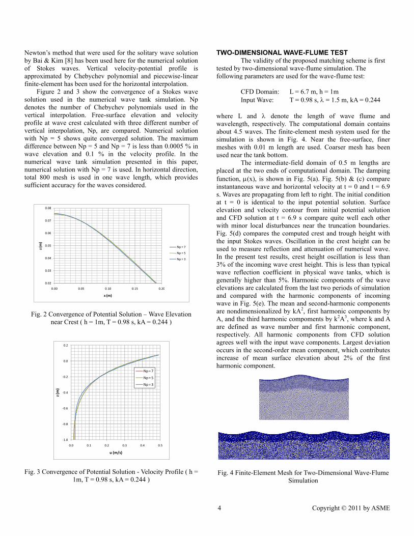
Figure 2 and 3 show the convergence of a Stokes wavesolution used in the numerical wave tank simulation. Npdenotes the number of Chebychev polynomials used in thevertical interpolation. Free-surface elevation and velocityprofile at wave crest calculated with three different number ofvertical interpolation, Np, are compared. Numerical solutionwith Np = 5 shows quite converged solution. The maximumdifference between Np = 5 and Np = 7 is less than 0.0005 % inwave elevation and 0.1 % in the velocity profile. In thenumerical wave tank simulation presented in this paper,numerical solution with Np = 7 is used. In horizontal direction,total 800 mesh is used in one wave length, which providessufficient accuracy for the waves considered.

Fig. 2 Convergence of Potential Solution – Wave Elevationnear Crest ( h = 1m, T = 0.98 s, kA = 0.244 )

Fig. 3 Convergence of Potential Solution - Velocity Profile ( h =1m, T = 0.98 s, kA = 0.244 )

TWO-DIMENSIONAL WAVE-FLUME TESTThe validity of the proposed matching scheme is first

tested by two-dimensional wave-flume simulation. Thefollowing parameters are used for the wave-flume test:

CFD Domain: L = 6.7 m, h = 1mInput Wave: T = 0.98 s, = 1.5 m, kA = 0.244

where L and denote the length of wave flume andwavelength, respectively. The computational domain containsabout 4.5 waves. The finite-element mesh system used for thesimulation is shown in Fig. 4. Near the free-surface, finermeshes with 0.01 m length are used. Coarser mesh has beenused near the tank bottom.

The intermediate-field domain of 0.5 m lengths areplaced at the two ends of computational domain. The dampingfunction, (x), is shown in Fig. 5(a). Fig. 5(b) & (c) compareinstantaneous wave and horizontal velocity at t = 0 and t = 6.9s. Waves are propagating from left to right. The initial conditionat t = 0 is identical to the input potential solution. Surfaceelevation and velocity contour from initial potential solutionand CFD solution at t = 6.9 s compare quite well each otherwith minor local disturbances near the truncation boundaries.Fig. 5(d) compares the computed crest and trough height withthe input Stokes waves. Oscillation in the crest height can beused to measure reflection and attenuation of numerical wave.In the present test results, crest height oscillation is less than3% of the incoming wave crest height. This is less than typicalwave reflection coefficient in physical wave tanks, which isgenerally higher than 5%. Harmonic components of the waveelevations are calculated from the last two periods of simulationand compared with the harmonic components of incomingwave in Fig. 5(e). The mean and second-harmonic componentsare nondimensionalized by kA2, first harmonic components byA, and the third harmonic compoments by k2A3, where k and Aare defined as wave number and first harmonic component,respectively. All harmonic components from CFD solutionagrees well with the input wave components. Largest deviationoccurs in the second-order mean component, which contributesincrease of mean surface elevation about 2% of the firstharmonic component.

Fig. 4 Finite-Element Mesh for Two-Dimensional Wave-FlumeSimulation

0.02

0.03

0.04

0.05

0.06

0.07

0.08

0.00 0.05 0.10 0.15 0.20

z(m

)

x (m)

Np = 7

Np = 5

Np = 3

-1.0

-0.8

-0.6

-0.4

-0.2

0.0

0.2

0.0 0.1 0.2 0.3 0.4 0.5

z(m

)

u (m/s)

Np = 7

Np = 5

Np = 3


(a) Damping function

(b) Initial wave elevation and horizontal-velocity contour at t = 0.0 s

(c) Wave elevation and horizontal-velocity contour at t = 6.9 s

(d) Wave crest and trough height at wave gauges

(e) Harmonic components of wave elevation at wave gauges

Fig. 5 Two-dimensional Wave-Flume Simulation Results ( h = 1m, T = 0.98 s, kA = 0.244 )

0

2

4

6

8

-3.5 -3 -2.5 -2 -1.5 -1 -0.5 0 0.5 1 1.5 2 2.5 3 3.5

x (m)

Damping m(x)

-0.06

-0.04

-0.02

0.00

0.02

0.04

0.06

0.08

0.10

-3 -2 -1 0 1 2 3

z(m

)

x (m)

Computed Crest

Computed Trough

Input Crest

Input Trough

0

0.2

0.4

0.6

0.8

1

1.2

-3 -2 -1 0 1 2 3

Am

pli

tud

e(N

on

-dim

.)

x (m)

0th (Comp.)

1st (Comp.)

2nd (Comp.)

3rd (Comp.)

0th (Input)

1st (Input)

2nd (Input)

3rd (Input)


DIFFRACTION BY A TRUNCATED CYLINDERThe run-up of Stokes wave on a truncated circular

cylinder, with radius a = 0.15 m and draft d = 0.87 m, has beensimulated. Two wave system with the following parameters aresimulated:

Case 1: T = 1.2 s, = 2.25 m, kA = 0.244

Case 2: T = 1.7 s, = 4.5 m, kA = 0.16, 0.20, 0.22, 0.23

The Case 1 wave is the same wave system that was tested in thetwo-dimensional wave-flume simulation. Case 2 waves arewith wave length two times longer than Case 1. Three differentwave steepness are tested. The simulated results are comparedwith the model test data and the second-order WAMIT resultsfrom [4].

(a) Plan View

(b) Side View

Fig. 6 Finite-Element Mesh for a Rectangular Numerical WaveTank

(a) Plan View

(b) Side View

Fig. 7 Finite-Element Mesh for a Circular Numerical WaveTank

Rectangular domain with the size

L x B x h = 3 m x 1.5 m x 1.5 m

has been used for the Case 1. For Case 2 wave, circular domainwith

Radius = 1.5 m, h = 1.5 m

has been used. The radius of circular domain is one third of theincoming wave length. Fig 6 and 7 show the finite-elementmesh for the two cases, respectively.

Fig. 8 shows the contour plots of free-surface elevation forCase 1 at three different time steps. It can be seen that waveenters and exits the computational domain with little reflectionfrom the outer boundary.


(a) t = 9.06 s

(b) t = 9.19 s

(c) t = 9.68 s

(d) t = 9.80 s

Fig. 8 Surface-Elevation Contour in Rectangular NumericalWave Tank ( h = 1.5 m, a = 0.15 m, T = 1.2 s, /a = 15.9, kA =0.244, H/a = 1.2)

(a) t = 8.94 s

(b) t = 9.19 s

(c) t = 9.43 s

(d) t = 9.68 s

Fig. 9 Free-Surface Elevation Contour in Circular NumericalWave Tank ( h = 1.5 m, a = 0.15 m, T = 1.7 s, /a = 30.4, kA =0.2)


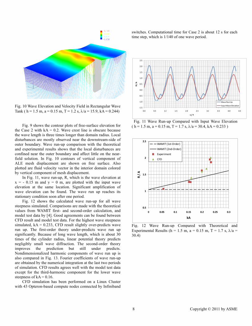
Fig. 10 Wave Elevation and Velocity Field in Rectangular WaveTank ( h = 1.5 m, a = 0.15 m, T = 1.2 s, /a = 15.9, kA = 0.244)

Fig. 9 shows the contour plots of free-surface elevation forthe Case 2 with kA = 0.2. Wave crest line is obscure becausethe wave length is three times longer than domain radius. Localdisturbances are mostly observed near the downstream-side ofouter boundary. Wave run-up comparison with the theoreticaland experimental results shows that the local disturbances areconfined near the outer boundary and affect little on the near-field solution. In Fig. 10 contours of vertical component ofALE mesh displacement are shown on free surface. Alsoplotted are fluid velocity vector in the interior domain coloredby vertical component of mesh displacement.

In Fig. 11, wave run-up, R, which is the wave elevation atx = - 0.15 m and y = 0 m, are plotted with the input waveelevation at the same location. Significant amplification ofwave elevation can be found. The wave run up reaches itsstationary condition soon after one period.

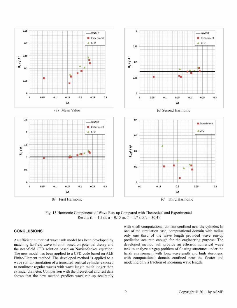
Fig. 12 shows the calculated wave run-up for all wavesteepness simulated. Comparisons are made with the theoreticalvalues from WAMIT first- and second-order calculation, andmodel test data by [4]. Good agreements can be found betweenCFD result and model test data. For the highest wave steepnesssimulated, kA = 0.233, CFD result slightly over-predicts waverun up. The first-order theory under-predicts wave run upsignificantly. Because of long wave length, which is about 30times of the cylinder radius, linear potential theory predictsnegligibly small wave diffraction. The second-order theoryimproves the prediction but still under predicts.Nondimensionalized harmonic components of wave run up isalso compared in Fig. 13. Fourier coefficients of wave run-upare obtained by the numerical integration at the last two periodsof simulation. CFD results agrees well with the model test dataexcept for the third-harmonic component for the lower wavesteepness of kA = 0.16.

CFD simulation has been performed on a Linux Clusterwith 43 Opteron-based compute nodes connected by Infiniband

switches. Computational time for Case 2 is about 12 s for eachtime step, which is 1/140 of one wave period.

Fig. 11 Wave Run-up Compared with Input Wave Elevation( h = 1.5 m, a = 0.15 m, T = 1.7 s, /a = 30.4, kA = 0.233 )

Fig. 12 Wave Run-up Compared with Theoretical andExperimental Results (h = 1.5 m, a = 0.15 m, T = 1.7 s, /a =30.4)

-1.5

-1.0

-0.5

0.0

0.5

1.0

1.5

2.0

2.5

0.0 0.5 1.0 1.5 2.0 2.5 3.0 3.5 4.0 4.5

R/

A

t / T

Wave Run Up

Input Wave Elevation

0.5

1

1.5

2

2.5

0 0.05 0.1 0.15 0.2 0.25 0.3

R/

A

kA

WAMIT (1st-Order)

WAMIT (2nd-Order)

Experiment

CFD


(a) Mean Value

(b) First Harmonic

(c) Second Harmonic

(c) Third Harmonic

Fig. 13 Harmonic Components of Wave Run-up Compared with Theoretical and ExperimentalResults (h = 1.5 m, a = 0.15 m, T = 1.7 s, /a = 30.4)

CONCLUSIONS

An efficient numerical wave tank model has been developed bymatching far-field wave solution based on potential theory andthe near-field CFD solution based on Navier-Stokes equation.The new model has been applied to a CFD code based on ALEFinite-Element method. The developed method is applied to awave run-up simulation of a truncated vertical cylinder exposedto nonlinear regular waves with wave length much longer thancylinder diameter. Comparison with the theoretical and test datashows that the new method predicts wave run-up accurately

with small computational domain confined near the cylinder. Inone of the simulation case, computational domain with radiusonly one third of the wave length provided wave run-upprediction accurate enough for the engineering purpose. Thedeveloped method will provide an efficient numerical wavetank to analyze air-gap problem of floating structures under theharsh environment with long wavelength and high steepness,with computational domain confined near the floater andmodeling only a fraction of incoming wave length.

0

0.05

0.1

0.15

0.2

0.25

0 0.05 0.1 0.15 0.2 0.25 0.3

R0

a/

A2

kA

WAMIT

Experiment

CFD

0

0.5

1

1.5

2

2.5

0 0.05 0.1 0.15 0.2 0.25 0.3

R1

/A

kA

WAMIT

Experiment

CFD

0

0.25

0.5

0.75

1

0 0.05 0.1 0.15 0.2 0.25 0.3

R2

a/

A2

kA

WAMIT

Experiment

CFD

0

0.1

0.2

0.3

0.4

0.1 0.15 0.2 0.25 0.3

R3

a2/

A3

kA

Experiment

CFD


ACKNOWLEDGMENTSThe authors would like to thank Technip for permittingpublication of this paper.

REFERENCES

[1] Kim, J.W., Kyoung, J.H., Ertekin, R.C. and Bai, K.J. 2006“Finite-Element Computation of Wave-Structure Interactionbetween Steep Stokes Waves and Vertical Cylinders,” J.Waterway, Port, Coastal, and Ocean Engineering, Vol. 132,No. 5, pp. 337-347.

[2] Kim, J.W., Kyoung, J.H., Bai, K.J. and Ertekin, R.C.2004 “A Numerical Study of Nonlinear Diffraction Loadson Floating Bodies due to Extreme Transient Waves,” 25th

Symposium on Naval Hydrodynamics, St. John’s,Newfoundland and Labrador, CANADA

[3] Kriebel, D. L. 1992 Nonlinear Wave Interaction with aVertical Circular Cylinder – Part II: Wave Run-Up, OceanEngng, 19(1), 75-99.

[4] Morris-Thomas, M.T. and Thiagarajan, K.P. 2004, “TheRun-Up on a Cylinder in Progressive Surface Gravity Waves:Harmonic Components,” Appl. Ocean Research, Vol. 26, pp.98-113.

[5] Swan, C., Taylor, P. H. and van Langen, H. "Observation ofwave-structure interaction for a multi-legged concreteplatform" Applied Ocean Research, 19, 1997, pp. 309-327.

[6] Clauss G.F., Cshmittner, C.E. and Stuck R., 2005“Numerical Wave Tank – Simulation of Extreme Waves for theInvestigation of Structural Responses,” Proc. OMAE 2005,Halkidiki, Greece.

[7] Donea, J., “Arbitrary Lagrangian-Eulerian finite elementmethods”, Computational Methods for Transient Analysis,Elseiver Science Publisher, pp. 474-516, 1983.

[8] Bai, K.J. and Kim, J.W. 1995 “A Finite-Element Method forFree-Surface Flow Problems,” Theor. Appl. Mech. Vol. 1, No.1, pp. 1-27.

[9] AcuSolve, General Purpose CFD Software Package,Release 1.7f, ACUSIM Software, Mountain View, CA, 2008.

numerical wave tank analysis of wave run-up on a …

Documents