water wave decay and run-up in the numerical water wave tank

* Corresponding author.

1944-3994/1944-3986 © 2020 Desalination Publications. All rights reserved.

Desalination and Water Treatment www.deswater.com

doi: 10.5004/dwt.2020.25290

188 (2020) 375–389June

Water wave decay and run-up in the numerical water wave tank

Gang Xua, Guichao Niua, Tong Lub, Haoyi Lic, Shuqi Wanga,*aSchool of Naval Architecture and Ocean Engineering, Jiangsu University of Science and Technology, Zhenjiang 212003, China, email: [email protected] (S. Wang) bGuangzhou Marine Engineering Corporation, Guangzhou 510220, China cThe 705 Research Institute, China Shipbuilding Industry Corporation, Xi’an 710077, China

Received 8 June 2019; Accepted 12 December 2019

a b s t r a c tWave is a common phenomenon in the sea environment, which is closely related to ships and ocean engineering. This work is based on ANSYS FLUENT 18.0 and the numerical wave tank (NWT) with water wave-making and water wave-eliminating module were established. Using the user-defined functions program in the solver, velocity inlet boundary, and piston-type wavemakers have been implemented. The second-order Stokes water wave has been simulated and compared. The water wave elimination is employed by modifying the source term of the momentum equation in the wave elimination region (End of the tank). Finally, the character of water wave decay in the NWT was analyzed, and the verification of run-up in the water wave tank has been presented by the standard calculation proposed by the International Towing Tank Conference.

Keywords: Numerical wave tank; Wavemaker; Water wave decay; Run-up

1. Introduction

The wave surface is the interface between water and air that changes with time and is impermeable to each other in the numerical viscously water wave tank. Since the flow velocity in the flow field is much smaller than the speed of sound, both air and water can be treated as an incompress-ible fluid. Actually, the effort of the numerical method of generating wave is to use the numerical simulation method to reconstruct the free surface shape and position with time and the wave is according to the corresponding wave the-ory. The virtual wave tank (Numerical Wave Tank, NWT) for complex offshore structures by numerical simulation will be able to obtain detail information of the flow field that cannot be obtained by the physical model test [1].

Wave-making and wave-elimination are key technolo-gies in the establishment of NWT. In recent years, research-ers have conducted a lot of work on the wave-making and wave-eliminating methods in the NWT. Prasad [2] used

ANSYS CFX and the piston-type wavemaker method for the simulation of the regular wave. The accuracy of the numer-ical method is verified by comparison with the experimen-tal results; Zou [3] and Liu [4] used a moving boundary to simulate the motion of wavemaker, and successfully gener-ated regular waves; Peng et al. [5] adopted the wave-making and wave-eliminating technology by adding source terms to the momentum equation, and numerically simulated linear and nonlinear waves; Li et al. [6] studied the complete non-linear wave-structure interaction of fixed floating structures under regular and irregular waves in a two-dimensional NWT by the piston-type wavemaker; Xin [7] compared the wavemaker of BEM with that of the piston-type wavemaker based on FLUENT, the simulated results of two-dimen-sional viscous NWT agree well with those of BEM; Guo et al. [8] simulated the interaction between irregular waves and seawall based on Navier-Stokes equation and Smagorinsky turbulence model, and solved the reflection wave by ana-lytic relaxation method; Finnegan [9] used ANSYS CFX as

G. Xu et al. / Desalination and Water Treatment 188 (2020) 375–389376

a platform to establish a rocker-type numerical tank based on the Navier-Stokes equation, and analyzed the velocity of the fluid particle and the applicable possibility of the tank; Wang et al. [10] proposed three kind of damping functions to describe the variation of damping in the elimination area and summarize the relevant laws when studying the regular wave elimination problem under different conditions; Fan et al. [11] verified the accuracy of the NWT using velocity inlet wavemaker and damping source term based on the OpenFOAM; Chen and Hsiao [12] established two-dimen-sional numerical tank by mass source wave-making and damping wave-eliminating technology, and extended it to three-dimensional wavemaker. The results show that the method can effectively generate and eliminate waves in the tank. Although there are many methods for generating and eliminating waves, the NWT cannot avoid the wave decay problems because of viscosity and numerical dissipation. Yang and Shi [13] mentioned that the wave decay problem is common in NWT, especially in short-wave simulations, and the influence factors of wave decay are obtained through theoretical analysis; Liu et al. [14] studied the wave decay in two-dimensional condition by the piston-like wave- making; Zhao et al. [15] used the same method to find the rule of wave decay and to obtain the corrected technology.

When the wave meets the structure, a significant run-up will occur near the structure due to the interaction. The wave run-up will likely create green water and slamming, which may cause damage to the structure. In the design of marine structures, it is necessary to ensure that the structure has sufficient deck height, however, deck height increased will result in costs and other stability issues, and it is useful to estimate the wave run-up. Although many researchers predicted successfully the run-up and air gap by used potential flow theory, it is not accurate enough as the viscosity effect has been considered. With the develop-ment of computing technology, it is possible to predict the run-up and air gap by used viscous flow theory. Research carried out a detailed experimental study on wave run-up and the air gap response of semi-submersible platforms [16]. A predicted the negative air gap of the semi-submers-ible platform [17]. A studied the near-field interaction effect of a four-column semi-submersible platform based on the viscous flow theory [18,19].

The present work will set a numerical water wave tank based on the commercial software ANSYS FLUENT. Both velocity inlet boundary and piston-type wavemaker will be using the user-defined functions (UDF) in the paper, it can be loaded by FLUENT to achieve the functionality which the user wants to have. The user can code functions using

the C computer language based on the FLUENT command. The boundary conditions, the momentum equation source terms, and the phase distribution can be set. The UDF com-mands used in this paper have the module of DEFINE_PROPERTY, DEFINE_SOURCE, and EFINE_CG_MOTION.

In this work, we will use the above module to write the wave-making and the wave-eliminating function of the NWT. The results will be verified and analyzed by the two kinds of wave-making methods, velocity inlet boundary, and piston-type wavemaker. Then based on the established numerical water wave tank, the wave decay problem in the tank is studied by the piston-type wave-making method. Finally, based on the standard examples presented by the International Towing Tank Conference (ITTC), the accuracy of Run-up on the specified cylinder in the NWT are com-pared and verified.

2. Numerical water wave tank and boundary condition setting

2.1. Numerical model and mesh discretization

The numerical water wave tank was built based on the fluid analysis module in ANSYS FLUENT 18.0. The total length of the tank is 60 m, width is 6 m, water depth is 6 m, and the height of the air part is 2 m. The left of the tank is set for wavemaker, the right is provided as a wave-eliminating region with a length of 20 m and the middle of the tank is a working area for capturing wave height and run-up on the cylinder. The entire wave tank is shown in Fig. 1.

The computational domain is meshed by ANSYS ICEM. The grid is divided into at least 35 parts along the wave propagation direction in each wavelength, encryption is adopted in the region where it is close to free surface, and the diverging grids are used where the place is away from the free surface. In addition, the size of the grid is gradu-ally increased along the wave propagation direction in the wave-eliminating area, and the wave energy dissipation can be increased. The meshing of the XOZ plane is shown in Fig. 2.

2.2. Boundary condition setting

In fact, the setting of boundary conditions is not exactly the same when using different wave-making meth-ods. In general, the upper boundary is taken as a pres-sure-inlet, the bottom boundary is a wall, the left, and right side boundaries are set as symmetry. The setting of the left-end boundary of the wave-making area and the right-end boundary of the wave-eliminating area needs

Fig. 1. Sketch of numerical water wave tank.

377G. Xu et al. / Desalination and Water Treatment 188 (2020) 375–389

to be adjusted according to the wave-making method and models. The other boundaries are also adjusted accordingly to the calculation which can be performed stably.

• Inlet conditions

The inlet condition, which belongs to a virtual condition, it should be set based on the wave theory at the entrance.

• Wall conditions

For non-sliding rigid wall, the velocity of fluid flow on the rigid wall is 0 when the wall is stationary.

• Symmetry conditions

For the problem of the physical symmetry of the flow field, the computational complexity can be reduced by set-ting the symmetrical boundary. On the symmetrical bound-ary conditions, the fluid is impermeable.

• Outlet conditions

The computational domain is limited in size, so there must have fluid inflow and outflow in the process of calcula-tion. It ensures that the density, velocity, and pressure remain unchanged at the outlet for the simulation.

The velocity component in the flow field is calculated from time t = 0 s. The pressure-velocity coupling method is solved iteratively by used the Pressure Implicit Split Operator method. Wave generation at the left-end boundary can be implemented by the UDF in the ANSYS FLUENT. The basic parameters of the simulation case are shown in Table 1.

3. Numerical methods of wave-making and wave-eliminating

In the NWT, wave-making and wave-eliminating technol-ogies are considered as a basic problem for open boundary simulation. If the end of the tank is a solid wall, there is no need to set the wave-eliminating condition. The wave-mak-ing methods are as follows: (1) Velocity inlet boundary,

the velocity components in the horizontal, and the vertical direction are inputted directly according to the wave the-ory. (2) Similar to physical wavemaker, for example, the pis-ton-type wavemaker which can generate wave by simulat-ing the wave-making plate motion. (3) Source wave-making method, the method can be divided into the mass source and momentum source wavemaker, implement wave generation by modifying the source term of the momentum equation. In addition, the types of wave-eliminating methods are arti-ficial transmission boundary, porous medium and artificial damping wave elimination. The previous study used the improved artificial damping wave-eliminating method to simulate wave propagation in the tank [20,21]. A two-dimen-sional sketch of the NWT is given in Fig. 3, the inlet boundary for wavemaker is on the left side of the tank, the right side of the tank is for the outlet boundary, and the middle part of the tank is the work area, the virtual wave height monitor can be set to output the time history results at the specified location.

3.1. Velocity inlet boundary wavemaker

The velocity boundary wavemaker is presented by set-ting the velocity at a specified point at the inlet boundary continuously based on corresponding wave theory. The wave then will propagate in the NWT. The linear wave equation for a finite water depth can be given by Eq. (1).

η ω ϕ= − +( )A kx tcos (1)

The corresponding velocity distribution can be obtained in Eqs. (2) and (3).

u Ak z dkd

k x ct x=+( )

−( )ωch

shin directioncos (2)

w Ak z dkd

k x ct z=+( )

−( )ωsh

shin directionsin (3)

where A is amplitude, ω is circular frequency, d is water depth, c is wave speed, k is wave number, u is velocity

Fig. 2. Mesh discretization on XOZ plane.

Table 1Parameters of the wave simulation case

Wave height Wavelength Time step Time Initial turbulent energy Rate of turbulent dissipation

H/m l/m Dt/s t/s k/m2 × s2 ε/m2 × s2

0.14 8 0.01 40 0.001024 2.5799e–5


component of the horizontal direction, and w is velocity component of the vertical direction.

When using the velocity inlet wavemaker, firstly, we need to set the wave-making zone as the velocity inlet and to set the velocity component of the linear wave as the inlet conditions of the NWT. This work uses UDF programming provided by FLUENT and the UDF predefined macro is DEFINE_PROFILE (name, thread, index). In this work, the aim is to simulate waves accurately, the code to capture the wave surface is also included in the UDF, which is the macro DEFINE_PROFILE (vof_function, thread, index).

By setting the wave height monitor of 0.5 and 1.0 λalways from the inlet boundary in the tank, we obtained the time history results and compared with theoretical values in Fig. 4. It shows that the two curves are very close and almost have the same trend.

We can see from Fig. 4 that the wave will be stable after certain period propagation in the tank. We also can find that the wave height has attenuation, and the troughs will decay faster than the crest. In addition, we find that the wave elevation both at the crest and at the trough is big-ger than the theoretical values while the input velocity-type

wavemaker is used. This phenomenon will become obvi-ously when the simulated case of wave height is increased. The main reason for this phenomenon is caused by the unequal flow between the inlet and outlet boundary, it may be improved by velocity correction at the outlet boundary or setting an additional flow out condition for the outlet boundary, it mostly depends on the numerical experience. Although there have some problems with the velocity inlet boundary wave-making method, the accuracy, and simple implementation are better than other methods when we simulate a linear wave. Therefore, this method is still a pop-ular wave-making tool and is widely used in the NWT.

3.2. Similar with physical wavemaker

3.2.1. Linear wave theory and results

The imitation of physics wavemaker is also called the dynamic boundary wavemaker, it is applied by simulat-ing the motion of the piston, there are two main types of wave-making machines, flat-type and piston-type wave-maker, however, the piston-type wave-making method

Fig. 3. Sketch of 2D NWT.

0 5 10 15 20 25 30 35 40-0.10

-0.05

0.00

0.05

0.10 x=0.5λ theoretical values

H / m

t/s

0 5 10 15 20 25 30 35 40-0.10

-0.05

0.00

0.05

0.10 x=λ theoretical values

H /m

t/s

(a)

(b)

Fig.4.Comparisonofwaveelevationbyvelocityboundaryinletconditionwiththetheoreticalvalues.(a)0.5λand(b)1.0λalwaysfrom inlet boundary.


is easier to implement and the piston-type wave-making method is used more frequently for NWT with finite water depth. For linear waves, Eq. (6) can be obtained by Eqs. (4) and (5), and linear wave profile in the time domain can be obtained by theoretical calculation.

The formula of the piston-type plate displacement:

X t S t( ) = − ( )2cos ω (4)

The formula of the plate speed:

U t S t( ) = ( )ωω

2cos (5)

The formula of wave height:

η ωx t H kx t, cos( ) = −( )2

(6)

According to the wave-making theory of linear wave, it satisfies the relationship of Eq. (7) between the motion dis-placement S0 of the plate and linear wave height H:

HS

kdkd kd0

242 2

=( )

+ ( )sinh

sin (7)

where k is the wavenumber and d is the water depth of the calculation domain.

For the piston-type wavemaker, the left boundary of the wave-making area and the right boundary of the wave-eliminating area are both set as a rigid non-slip

wall, and the other settings are consistent with the veloc-ity boundary. The wave-making plate is one degree of motion in x direction, which can be implemented by the macro of DEFINE_CG_MOTION (piston, dt, vel, omega, time, dtime), as presented in the Appendix A. In order to find the stable results and avoid the unstable ini-tial condition, it is necessary to add a smoothing function (modulation function) in the first two periods of the pis-ton motion, which can be described by Eq. (8), where T is motion period of the plate.

Fuctime time

time=

≤

>

2

2

1 2

TT

T

,

, (8)

The numerical simulation of the linear wave can be done according to the above setting, and the time history of wave height at a specified position is shown in Fig. 5. Compared with the velocity inlet boundary wave-making method, the wave history, present here, is more stable and does not have the phenomenon to upraise the wave height. Moreover, the piston-type wavemaker is used to simulate wave and structure interaction problem, which has less affection by the reflected waves [22,23]. We will use this method for the verification of Run-up prediction later.

3.2.2. Second-order Stokes wave theory and results

When the wave nonlinearity cannot be ignored, a significant error will occur when using the piston-type wave-making method to simulate a steep wave. Therefore, higher-order wave-making modes must be summarized to simulate nonlinear waves. In Madsen’s wave-making exper-iment [24], it was found that the small-amplitude wave

0 5 10 15 20 25 30 35 40

-0.08

-0.04

0.00

0.04

0.08

0.12

t/s

x=0.5λ theoretical values

H /m

(a)

0 5 10 15 20 25 30 35 40

-0.08

-0.04

0.00

0.04

0.08

0.12 x= λ theoretical values

H /m

t/s

(b)

Fig.5.Comparisonofwaveelevationbypiston-typewavemakerwiththetheoreticalvalues.(a)0.5λand(b)1.0λalwaysfromleftboundary.


was generated by the linear piston-type wave-making the-ory, it contains the second-order wave component, which causes the wave unstable during the propagation. Madsen revised the formula of the piston-type plate motion and the updated plate motion has been verified by experimental test. The displacement of the second-order wave-making plate is described in Eq. (9).

X t S t Hdn kd

n t( ) = − + −

cos

sinhsinω ω

23

4 22

12 (9)

In order to make the dynamic mesh more stable and avoid the error in the first-cycle wave-making period, the phase angle has been changed and the wave is in the sine format for input. The formula is presented in Eq. (10).

X t S t Hdn kd

nt( ) = − ( ) + −

sin

sinhsinω ω

43

4 22

12

1 (10)

Here: n kdkd

SHn

kd111

21 2

2 2= +

=

sin,

tanh.

The formula of wave height can be obtained in Eq. (11).

η ω ω= −( ) ++( )

−( )H kx t kH kdkd

kx t2 16

2 22

2

3coscosh

sinhcos (11)

According to the second-order wave-making theory proposed by Madsen, the motion function of the plate is coded in the UDF, and the second-order Stokes wave can be simulated by moving the boundary. In order to verify the method in this paper, the numerical model and calcu-lation parameters were set according to the parameters in the Madsen experiment. The water depth, the period of plate motion, the amplitude of plate motion and the Ursell number are chosen d = 0.38 m, S = 0.061 m, T = 2.75, and

Ur = 27.2, respectively. The small-amplitude wave is stim-ulated by both the linear piston wave-making method and the second-order wave-making mode according to the above parameters.

In Fig. 6, the time history of wave height at a specified point (x = 5 m) has been presented. It can be seen that the result is inaccurate while the linear piston-type wave-mak-ing method is used, and the nonlinear effect is obvious as shown in Fig. 6a. The results have been greatly improved when the second-order wave-making mode is adopted and the stable results can be obtained, as shown in Fig. 6b. We also can find that the stable results agree well with experimental data, as shown in Fig. 7.

3.3. Numerical methods of wave-eliminating

3.3.1. Momentum source wave-eliminating

The basic principle of the momentum source wave-elim-inating method is applied by adding an artificial damping source term to the momentum equation. It is called an artifi-cial damping method. In the NWT, the momentum equation can be rewritten as Eqs. (12) and (13).

∂∂

+∂∂

+∂∂

= −∂∂

+∂∂

+∂∂

− ( )u

tu uxv uz

f px

ux

uz

x ux1 2

2

2

2ρµρ

µ (12)

∂∂

+∂∂

+∂∂

= −∂∂

+∂∂

+∂∂

− ( )w

tu wx

v wz

f pz

wx

wz

x wz1 2

2

2

2ρµρ

µ (13)

Here, p is pressure, µ is the viscosity coefficient, fx and fz are the source item, represents the components of each vector rectangular coordinate system in the x and z direc-tions, µ(x) is the coefficient for wave elimination, it has many types, the most common of which are linear and exponen-tial. The damping coefficient for the linear type is given in Eq. (14).

15 20 25 30 35 40

-0.02

0.00

0.02

0.04

H /m

Linear motion for piston

t/s

(a)

15 20 25 30 35 40-0.04

-0.02

0.00

0.02

0.04

H /m

t/s

Second-order motion for piston (b)

Fig. 6. Time history of wave elevation at x = 5 m for linear and second-order piston motion. (a) Linear piston wave making method and (b) second-order wave making mode.


µ αx

x x x x

x xx x

x x x( ) =

≤ ≥

−( )−( ) ≤ ≤

0 1 2

1

1 21 2

,

,

or

(14)

Here, x1 is the starting position of the wave-eliminating area, x2 is the end of the wave-eliminating area, α is anartificial parameter.

The elimination coefficient of exponential (I) is presented by Eq. (15).

µα

x

x xx xx x

x x x( ) =

≥

−−

−

≤ ≤

1 2

1

2 11 2

,

exp , (15)

We should note that when using the exponential elimi-nation coefficient, it only need to modify the momentum source term in the vertical direction and can avoid breaking the continuity of the flow. Besides the two types described in this article [25,26], there still has square root types, exponential type II, and squared type.

3.3.2. Porous medium wave-eliminating

Porous medium wave elimination is a kind of pseu-do-physical elimination, which is adding a momentum decay source term in the momentum equation and setting a porous medium region in the calculation region. The source term format is in Eq. (16).

S v C v vi i i= − +

µα

ρ212

(16)

Intheformula,thefirsttermistheviscouslossterm,1/αis the viscous drag coefficient, the second term is the inertia loss term, C2 is the inertia drag coefficient, C2 can be deter-mined by Eq. (17).

C kpx xx x

x x xi

ei e2

0

00=

−−

< <, (17)

where x0 and xe are the starting and ending positions of the wave-eliminating area, respectively. p is the porosity factor.

Since the porosity has a great influence on wave elim-ination and is not easy to control for a porous medium wave-eliminating method, therefore, the momentum source method is adopted in this section. Fig. 8 is the snapshot of the free surface after the calculation result is stable, it can be found that good results can be obtained by the method in this paper, and the surface almost reaches the still level due to the wave elimination of the damping zone at the end of the tank. Fig. 9 shows the wave profile with different time, it can be clearly seen from the figure that the damping zone is working to eliminate the wave and the wave energy has been dissipated.

4. Convergent study of the NWT

It is found that the decay of wave will occur and become seriously, whether the velocity boundary wave-making or the piston wave-making method.

In fact, in the process of simulating waves in the NWT, wave decay mainly exists in the two aspects of numerical decay and physical viscosity decay. The physical viscosity is decayed due to the influence of physical viscosity during the wave propagation, while the theoretical value of the wave surface is based on the potential flow theory, ignoring the viscous effect. The numerical decay probably derived from the following aspects: mesh size, solution format of volume fraction, free surface reconstruction scheme, and discretiza-tion scheme. In this paper, the linear wave with the wave height H =0.14andthewavelengthλ=8misanalyzedandstudied.

4.1. Mesh size

It is well known that the refinement of free-surface meshes can improve the accuracy of numerical results. A recent study mentioned that the number of mesh nodes should be greater than 10 in the wave height direction [27]. Mesh nodes in the wave height region are fixed to 15, and then three cases will be considered: the mesh ratio (length/width) is 1/3, 1/6, and 1/12. Fig. 10 shows the comparison of the time-history results with different mesh ratios at a spec-ifiedpoint(0.5λalwaysfromtheleftboundary).Itcanbeseen that when the ratio of the mesh is 1/12, the wave decay is obviously serious than that of 1/6 and 1/3.

4.2. Solution format of volume fraction

When solving the multiphase flow problem using the volume of fluid (VOF) method, the Fluent provides two solutions to solve the volume fraction: Implicit and Explicit.

0.0 0.5 1.0 1.5 2.0 2.5 3.0

-0.02

0.00

0.02

0.04

experimental result

t/s

simulation result

H /m

Fig. 7. Comparison of numerical results and theoretical data.

Fig. 8. Snapshot of the free surface.


When using the explicit solution to solve the problem, the volume fraction of the current time step is calculated from the calculation results of the previous time step, thus the time step should not be small enough. When the implicit solution is adopted, the volume fraction is a function of other quantities in the present time step. Both solutions have their own advantages, the explicit one can capture the wave sur-face more accurately, but due to the limitation of Coulomb number when setting the time step, a smaller time step must be set. If the time step size is too large, the Courant num-ber will always be greater than 1 in the calculation, and the calculation will be distorted. When implicit one is used to solve the problem, the time step is not affected seriously by the Courant number, thus the calculation efficiency is accelerated. Therefore, Fluent clearly points out in the User

Guide that the explicit solution is more accurate when it is concerned about the calculation process and the accuracy of the wave surface. The implicit formulation can satisfy the requirement when only the computational results are con-cerned, such as the force and motion of the structure. The detailed description of the two solutions can be found in the Fluent Theory Guide. Fig. 11 shows a comparison between numerical simulation results and theoretical values. It can be seen that the explicit solution has good accuracy and the significant numerical decay can be found when the implicit solution is used.

4.3. Free surface reconstruction schemes

Free surface reconstruction means reconstructing the geometry of the free surface in the process of spatial discret-ization. Based on VOF method, the following technologies can reduce numerical decay: geo-reconstruct, high resolution interface capturing (HRIC), and compressive interface cap-turing scheme for arbitrary meshes (CICSAM).

Fig. 12 shows the time history results for different interface reconstruction schemes at a specified point (0.5λalwaysfromleftboundary).ItcanbeseenthatGeo-reconstruct and improved HRIC have better results than CICSAM. However, Geo-reconstruct is not applicable when an implicit solution is used. If the condition is not limited, the Geo-reconstruct scheme can be used for the NWT, oth-erwise, the HRIC scheme should be adopted.

4.4. Discretization schemes

Discretization scheme is an interpolation method for solving the quantities and their derivatives. It has first-order schemes and second-order schemes. The first-order scheme includes the central differential scheme, the first-order

-0.10

-0.05

0.00

0.05

0.10

0 10 20 30 40 50 60

flow time 28s

H /m

tank length/m

flow time 32s flow time 36s flow time 40s

Fig. 9. Wave profile in the wave tank at different time.

20 25 30 35-0.10

-0.05

0.00

0.05

0.10

H /m

explict implict theoretical values

t/s

Fig. 11. Comparison of theoretical values and numerical results with different solution format of volume fraction.

20 25 30 35 40

-0.08

-0.04

0.00

0.04

0.08 1/12 1/6 1/3 theoretical values

H /m

t/s

Fig. 10. Comparison of theoretical values and numerical results with different mesh ratio.


upwind scheme, and the exponential scheme. The second- order scheme is developed on the basis of the first-order scheme. The difference between the first-order scheme and the second-order scheme is that it not only uses the upstream node quantity but also uses the upper node. It mains that the calculation accuracy of the second-order scheme is better than the first-order scheme.

Fig. 13 is the comparison between the theoretical val-ues and the numerical results for different discretization schemes. It can be seen that the simulation accuracy of the second-order scheme is similar to the first-order scheme for the present case, however, the computational time of the sec-ond-order scheme is obviously longer than the first-order upwind scheme under the same time interval. If the com-putational conditions are allowed, the higher-order discret-ization scheme has an advantage to the first-order upwind scheme in the numerical simulation. It should be pointed out that the numerical results of high-order and low-order are similar if the ratio of mesh is relatively small. However, we always need to control the density of the mesh for wave-body interaction cases, which will result in a bigger ratio of the mesh. Therefore, the high-order discretization scheme will be adopted and can obviously improve the calculated accuracy.

5. Numerical analysis of wave decay along in the tank

In this paper, the related problems of wave decay in the working region of the tank have been analyzed. The NWT with a length of 70 m and a water depth of 15 m is setup, and the decay of the water waves under several linear inci-dent waves is investigated. Detailed parameters are shown in Table 2.

In order to analyze the wave decay along the length of the tank, the wave height monitor is set at x = 5, 10, 20, 30, 40 m from the wave-making boundary. Fig. 14 shows the wave decay procedure. Fig. 15 shows the relative attenuation ratio varying with wavelength.

We can find that the relative attenuation speed of the wave reduces with increasing wavelength as the short wave attenuation is significantly faster than the long waves. Therefore, the short wave is more sensitively affected by viscous and numerical models under the same fluid and solver. This conclusion is very useful for wave-structure interaction in field of ship and ocean engineering. Most of the simulation should consider the wave compensation when we set the inlet boundary condition, otherwise, we cannot have exact input wave conditions at the working region.

20 25 30 35 40-0.10

-0.05

0.00

0.05

0.10

H / m

HRIC CICSAM Geo theoretical values

t/s

Fig. 12. Comparison of theoretical values and numerical results with different interface reconstruct scheme.

20 25 30 35 40-0.10

-0.05

0.00

0.05

0.10 the first-order upwind scheme the second-order upwind scheme theoretical values

H /m

t/s

Fig. 13. Comparison of theoretical values and numerical results with different discretization schemes.

Table 2Parameters for each regular wave

Wave height (H/m) 0.06 0.08 0.1 0.12 0.14 0.16 0.18 0.22

Wave length (l/m) 4 5 6 7 8 9 10 12


6. Numerical verification of the tank by Run-up on the cylinder

The practical model is used for the simulation, the main dimension of the rectangular tank for the calculation is 921.6 m × 230.4 m × 300 m, as shown in Fig. 16. The radius of the cylinder is 16 m, the draft is 24 m, and the cylinder has been placed at 300 m away from the wave-making pis-ton-type plate. We set the zone with 1.5 times of wavelength for wave elimination.

6.1. Domain discretization and boundary conditions

The structured grid is used to discretize the whole domain. In order to improve the stability of the dynamic mesh and avoid negative meshes during the calculation, it is necessary to do that the mesh size is consistent in the wave-making area. To satisfy the requirement of standard wall conditions, it is necessary to encrypt the mesh near the cylinder. In this case, the first layer of the grid is set to 0.01 m, which can meet the requirements of simulation. The total number of grids is 1.34 million, as shown in Fig. 17.

In the experiment [28,29], wave-height gauges are installed around the cylinder to capture the wave Run-up. The exact location of the virtual wave-height monitor in this simulation is same with the experiment. Details and loca-tions are presented in Table 3 and Fig. 18. The parameters of the incident wave are given in Table 4. The boundary conditions and initial conditions in the numerical simula-tion are consistent with those mentioned above, wavemaker and wave-eliminating method are, respectively, performed by the piston-type wavemaker and artificial damping wave elimination.

6.2. Numerical results and discussion

Figs. 19 and 20 present the wave Run-up at A3, B3, and C3 in the time domain for incident waves I and II, respec-tively. From the numerical results, the highest Run-up occurs at 58 s, and then the results will be stable gradually. It means that the model with the corresponding setting in this work can obtain stable results in time domain.

We also can find that it has sudden change at the trough at position C3 when incident wave is Wave II, as shown in Fig. 20. It has the same phenomena with the experiment results given by Trulsen and Teigen [24]. According to the

0 10 20 30 400.04

0.06

0.08

0.10

0.12

λ=4

λ=5m

λ=6m

H

/m

x/m

λ=7m

0 10 20 30 400.12

0.14

0.16

0.18

0.20

0.22

λ=8m

λ=9m

λ=10m

H /

m

x/m

λ=12m

(a) (b)

Fig. 14. Wave decay along the wave tank. Range of wave length is (a) 4 m–7 m and (b) 8 m–12 m.

4 6 8 10 12

5

10

15

20

rela

tive

deca

y/%

λ/m

Fig. 15. Relative decay ratio (simulated value/H) with different wave length.

Fig. 16. Wave run-up on single cylinder in the NWT.


experimental data by Morris–Thomas, this phenomenon is called the secondary crest phenomenon, that is, the waves on both sides meet behind the cylinder, and the wave super-position will act on incoming waves, the secondary crest

(a) (b)

Fig. 17. Mesh of the domain for run-up simulation. (a) Mesh distribution for the domain and (b) Mesh distribution from top view.

Table 3Locations of virtual wave-height probes

Series number of wave-height monitor

Distance to the cylinder (m)

1 8.052 9.473 12.754 16

Fig. 18. Schematic diagram of wave-height gauges.

20 40 60 80 100 120 140-4

-2

0

2

4

H /m

t/s

(a)

20 40 60 80 100 120 140-4

-2

0

2

4

H /m

t/s

(b)

20 40 60 80 100 120 140-4

-2

0

2

4

H /m

t/s

(c)

Fig. 19. Time history of wave elevation at the prescribed point (Incident wave type is Wave (I). Wave-height monitor (a) A3, (b) B3, and (c) C3.


phenomenon will appear at the trough. This shows that the model established here can deliver the information in consistent with experiment.

Figs. 21 and 22 show the comparison of the calcu-lated values at the monitoring points with the results of the WAMIT based on the potential flow theory and the

experimental values provided by Trulsen and Teigen [24]. The accuracy of the present numerical calculation agrees well with the experimental data. It is worth mentioning that the waves acting on the cylinder will have a vortex behind it, which will affect the wave Run-up, however, this effect cannot be captured by the theory based on potential

20 40 60 80 100 120 140-6-4-20246

H /m

t/s

(a)

20 40 60 80 100 120 140-6-4-20246

H /m

t/s

(b)

20 40 60 80 100 120 140-6-4-20246

t/s

H /m

(c)

Fig. 20. Time history of wave elevation at the prescribed point (Incident wave is Wave II). Wave-height monitor (a) A3, (b) B3, and (c) C3.

0.7

0.8

0.9

1.0

1.1

1.2

1.3

1.4

1.5

C1 C2 C3 C4

experimental values

B1 B2 B3 B4

potential flow theory

A1 A2 A3 A4

η/(H

/2)

the number of wave height meter

viscous flow theory

Fig. 21. Comparison of wave Run-up on the cylinder (Incident wave is Wave I).

0.8

0.9

1.0

1.1

1.2

1.3

1.4

1.5

1.6

1.7

1.8

1.9

A4B4C4 B3B2B1

η/(H

/2)

viscous flow theory

the number of wave height meterC3C2

C1

experimental values

A3A2A1

potential flow theory

Fig. 22. Comparison of wave Run-up on the cylinder (Incident wave is Wave II).


flow, thus the simulation results by potential theory shows a significant error with viscous flow theory and physical test.

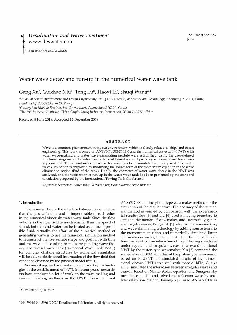
Fig. 23 shows the wave Run-up ratio at a different angle from A2 (180°) to E2 (0°), while the wave period is same and wave steepness is 1/30 and 1/16, respectively. It can be seen that the maximum wave Run-up will appear at the point A2 at 180°. It is in the front surface of the cylinder and faces to the incident wave, but the minimum values of wave Run-up will appear at the point D2 (45°). Comparing the maximum values of wave Run-up with two different wave steepness,

we can find that the bigger wave steepness the bigger wave Run-up will be presented while the incident wave period is fixed.

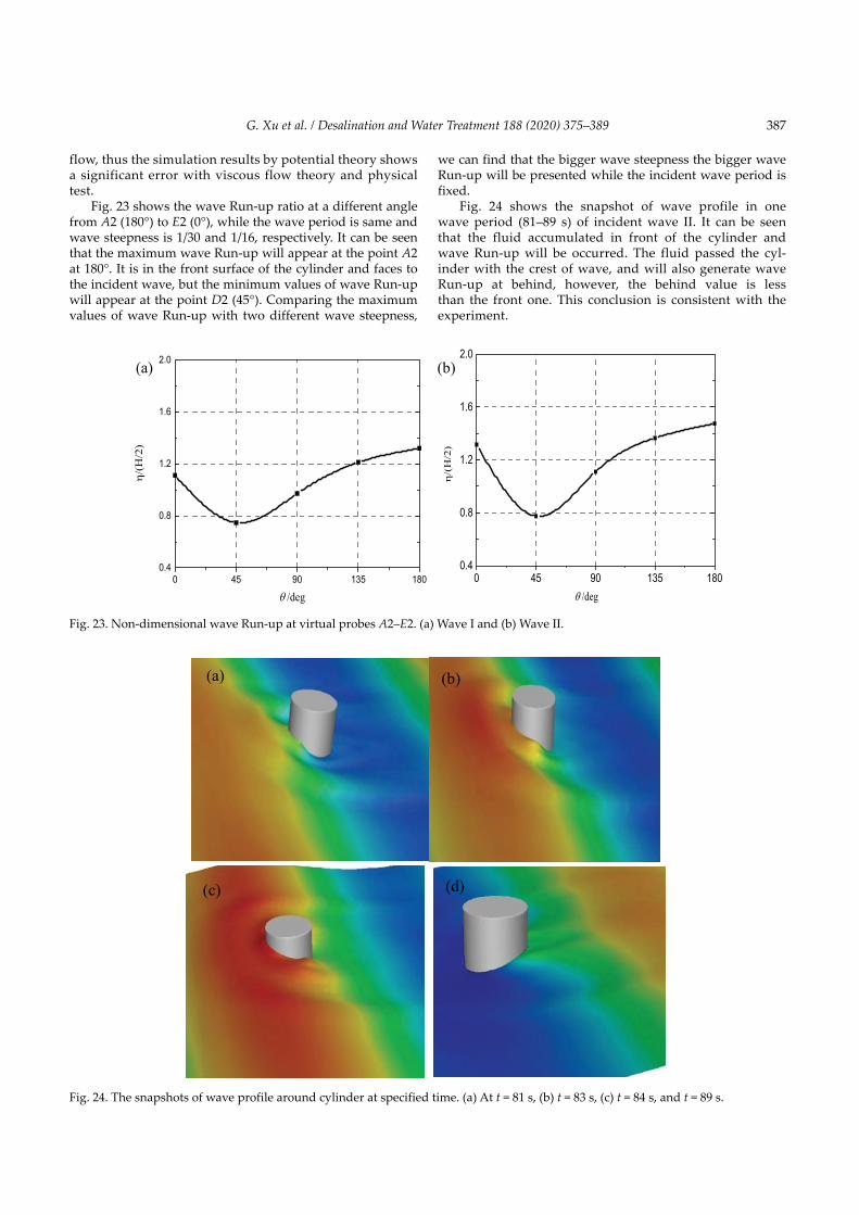
Fig. 24 shows the snapshot of wave profile in one wave period (81–89 s) of incident wave II. It can be seen that the fluid accumulated in front of the cylinder and wave Run-up will be occurred. The fluid passed the cyl-inder with the crest of wave, and will also generate wave Run-up at behind, however, the behind value is less than the front one. This conclusion is consistent with the experiment.

0 45 90 135 1800.4

0.8

1.2

1.6

2.0

η/(

H/2

)

θ /deg0 45 90 135 180

0.4

0.8

1.2

1.6

2.0

θ /deg

η/(

H/2

)

(a) (b)

Fig. 23. Non-dimensional wave Run-up at virtual probes A2–E2. (a) Wave I and (b) Wave II.

(a) (b)

(c) (d)

Fig. 24. The snapshots of wave profile around cylinder at specified time. (a) At t = 81 s, (b) t = 83 s, (c) t = 84 s, and t = 89 s.


7. Conclusions

In this paper, two different wave-making methods are used to analyze the NWT. The advantages and disadvan-tages of velocity inlet boundary and piston-type wave-maker are presented and the numerical results have been compared with theoretical values. It is found that the wave simulated by the piston-type wave-making method is more accurate and the stability is higher than the velocity inlet boundary. The wave energy will be lost during propaga-tion as viscosity effect and numerical dissipation. Then, the problem of wave decay along the numerical water wave tank is analyzed. The result shows that the rate of wave decay reduces with increasing wavelength as the short wave attenuation is significantly faster than the long waves. It means that the short wave is more sensitive than longwave during numerical simulation in the NWT. Finally, the interaction between wave and the fixed cylinder is ana-lyzed based on the standard model provided by ITTC com-mittee. Compared to the solutions by potential theory, the calculated results agree very well with the experimental data and the flow phenomenon is same as the experiment. It indicates that the present NWT with attached UDF has good accuracy, which can be used to simulate and ana-lyze the complex flow problem, such as air gap and multi- column interaction.

Acknowledgment

This work is supported by the National Natural Science Foundation of China (Grant No. 51709137, 51879125), Key University Science Research Project of Jiangsu (18KJA130001), Marine Equipment and Technology Institute of Jiangsu University of Science and Technology Funding Project (1174871801–17), Postgraduate Research and Practice Innovation Program of Jiangsu Province (KYCX18_2343, SJCX19_1187).

References[1] K. Xia, D.C. Wan, Numerical Analysis of Wave Evolution of

Semi-Island Reef and Motion Performance of Semi-Submersible Platform Based on CFD Method, The 14th National Conference on Hydrodynamics, Changchun, China, 2017.

[2] D.D. Prasad, M.R. Ahmed, Y.H. Lee, Validation of a piston type wave-maker using numerical wave tank, Ocean Eng., 131 (2017) 57–67.

[3] Z. Zou, Numerical simulation of nonlinear wave generated in wave flume by VOF technique, J. Hydrodyn., 11 (1996) 93–103.

[4] J.H. Liu, Making waves in 2-D numerical flume and feature analysis of the numerical waves, J. Sichuan Univ., 36 (2004) 28–31.

[5] J. Peng, Y. Liu, J. Liu, Research of numerical wave generation and wave absorption simulation based on momentum source method, Int. J. Digital Content Technol. Applic., 12 (2013) 23–28.

[6] Y. Li, M. Lin, Regular and irregular wave impacts on floating body, Ocean Eng., 42 (2012) 93–101.

[7] Y. Xin, Application Research of FLUENT+UDF Method in Numerical Wave Sink, Dalian University of Technology, Dalian, 2013.

[8] X.Y. Guo, B.L. Wang, H. Liu, Numerical simulation of irregular wave overtopping against a smooth sea dike, China Ocean Eng., 26 (2012) 153–166.

[9] W. Finnegan, J. Goggins, Numerical simulation of linear water waves and wave-structure interaction, Ocean Eng., 43 (2012) 23–31.

[10] Q.S. Wang, M.H. Li, L.Y. Zhang, Research on wave-eliminating method of numerical wave sink in the overweight environment, J. Hydrodyn. Ser. A, 6 (2017) 688–695.

[11] X. Fan, J.X. Zhang, Y. Liu, The Simulation of Numerical Wave Sink/Tank Based on OpenFOAM, National Conference on Hydrodynamics, Qingdao, 2014.

[12] Y.L. Chen, S.C. Hsiao, Generation of 3D water waves using mass source wavemaker applied to navier-stokes model, Coast. Eng., 109 (2016) 76–95.

[13] B. Yang, A.G. Shi, Research on wave numerical attenuation problem, ASME Press, 27 (2011) 43–58.

[14] J.H. Liu, Y.Q. Yang, H.Y. Zhang, Wave generation process and wave shape analysis of two-dimensional numerical water tank, Adv. Eng. Sci., 36 (2004) 28–31.

[15] Y. Zhao, R.Q. Zhu, Z. Liu, Study on the construction and viscous influence of three-dimensional numerical wave tank, Ship Sci. Technol., 36 (2014) 42–48.

[16] T.B. Shan, Research on the Mechanism of Wave Run-Up and Key Characteristics of Air Gap Response of Semi-Submersible Platform, Shanghai Jiao Tong University, Shang Hai, 2013.

[17] Z.D. Wang, M.J. Chen, H.J. Ling, Research on numerical calculation method of air gap of semi-submersible platform based on viscous flow theory, China Offshore Platform, 1 (2015) 35–41.

[18] M.M.H. Bhuiyan, K. Islam, K.N. Islam, M. Jashimuddin, Monitoring dynamic land-use change in rural–urban transition: a case study from Hathazari Upazila, Bangladesh, Geol. Ecol. Landscapes, 3 (2019) 247–257, doi: 10.1080/24749508.2018. 1556034.

[19] H.J. Ling, Z.D. Wang, M.J. Chen, Numerical calculation of near-field interference of semi-submersible platform based on viscous flow theory, China Offshore Platform, 33 (2018) 26–32.

[20] Y. Rajendran, R. Mohsin, Emission due to motor gasoline fuel in reciprocating lycoming O-320 engine in comparison to aviation gasoline fuel, Environ. Ecosyst. Sci., 2 (2018) 20–24.

[21] Y.F. Yu, Numerical Simulation of Waves and Analysis of Flow Field Structure, Harbin Institute of Technology, Harbin, 2013.

[22] H.B. Gu, H.B. Chen, Y.N. Luan, Numerical simulation of the motion of the piston like wave making plate, J. Waterw. Harbor, 32 (2011) 244–251.

[23] A. Omowumi, Electrical resistivity and hydrogeochemical evaluation of septic-tanks effluent migration to groundwater, Malaysian J. Geosci., 2 (2018) 01–10.

[24] O.S. Madsen, On the generation of long waves, J. Geophys. Res., 76 (1971) 8672–8683.

[25] P. Han, B. Ren, X.L. Li, Study of damping wave-eliminating of irregular wave in a numerical wave tank based on VOF method, J. Waterw. Harbor, 30 (2009) 15–19.

[26] L. Yang, H. Guo, H. Chen, L. He, T. Sun, A bibliometric analysis of desalination research during 1997–2012, Water Conserv. Manage., 2 (2018) 18–23.

Table 4Parameters for regular wavemaker

Series number of incident wave Wave height (m) Period (s) Wave steepness

Wave I 4.22 9 1/30Wave II 7.9 9 1/16


[27] H.W. Ling, Study on Wave-Making Method in a Numerical Tank, Harbin Institute of Technology, Harbin, 2009.

[28] K. Trulsen, P. Teigen, Wave scattering around a vertical cylinder: fully nonlinear potential flow calculations compared with low order perturbation results and experiment, ASME Conf. Proc., 2 (2002) 259–367.

[29] I. Sufiyan, J.I. Magaji, Modeling Flood hazard using swat and 3d analysis in Terengganu watershed, J. Clean WAS, 2 (2018) 19–24.

Appendix

A1 DEFINE_CG_MOTION

#include<stdio.h>#include“udf.h”#define A 0.07#define pi M_PI#define LW 8#define g 9.81#define h 6#define L0 40.0#define L1 60.0DEFINE_CG_MOTION(ban_moving, dt, cg_vel, cg_

omega, time, dtime){real u = 0;real ww = 0;real kk = 0;real S = 0;real cc = 0;real T = 0;kk = 2.0*pi/LW; cc = sqrt(g*tanh(kk*h)/kk); /*wave velocity*/ww = kk*cc; /*circle frequency*/T = 2.0*pi/ww;S = 0.5*A*(2*kk*h+sinh(2*kk*h))/pow(sinh(kk*h),2);if(time <= T){

u = ww*S*time*cos(ww*time)/(2*T);cg_vel[0] = u;

}

else{

u = ww*S*cos(ww*time)/2; cg_vel[0] = u;

}}/**********************************/DEFINE_SOURCE(xom_source,c,t,dS,eqn){real x[ND_ND];real source;real mu;C_CENTROID(x,c,t);if(C_U(c,t)<= 0){

mu = 2*pow(LW,0.5)*pow(((x[0]-L0)/(L1-L0)),2)*C_R(c,t);source = -mu*C_U(c,t);dS[eqn] = -mu;

}else{

mu = 0;source = 0;dS[eqn] = 0;

}return source;}/**********************************/DEFINE_SOURCE(zom_source,c,t,dS,eqn){real x[ND_ND];real source;real mu;C_CENTROID(x,c,t);

mu = 10*pow(LW,0.5)*pow(((x[0]–L0)/(L1–L0)),2)*C_R(c,t);source = –mu*C_W(c,t);

dS[eqn] = –mu;return source;}

water wave decay and run-up in the numerical water wave tank

Documents