nurul najihah mohamad - um students'...
TRANSCRIPT

INFERENCES FOR INTEGER-VALUED TIME SERIESMODELS
NURUL NAJIHAH MOHAMAD
FACULTY OF SCIENCEUNIVERSITY OF MALAYA
KUALA LUMPUR
2017
INFERENCES FOR INTEGER-VALUED TIME SERIESMODELS
NURUL NAJIHAH MOHAMAD
THESIS SUBMITTED IN FULFILMENTOF THE REQUIREMENTS
FOR THE DEGREE OF DOCTOR OF PHILOSOPHY
FACULTY OF SCIENCEUNIVERSITY OF MALAYA
KUALA LUMPUR
2017

UNIVERSITI MALAYA
ORIGINAL LITERARY WORK DECLARATION
Name of Candidate: NURUL NAJIHAH BINTI MOHAMAD (I.C./Passport No.:
)
Registration/Matrix No.:SHB 120008
Name of Degree:DOCTOR OF PHILOSOPHY (MATHEMATICS & SCIENCE PHI-
LOSOPHY)
Title of Project Paper/Research Report/Dissertation/Thesis (“this Work”):
INFERENCES FOR INTEGER-VALUED TIME SERIES MODELS
Field of Study:STATISTICAL TIME SERIES (STATISTICS)
I do solemnly and sincerely declare that:
(1) I am the sole author/writer of this Work;(2) This work is original;(3) Any use of any work in which copyright exists was done by way of fair dealing and for
permitted purposes and any excerpt or extract from, or reference to or reproductionof any copyright work has been disclosed expressly and sufficiently and the title ofthe Work and its authorship have been acknowledged in this Work;
(4) I do not have any actual knowledge nor do I ought reasonably to know that the makingof this work constitutes an infringement of any copyright work;
(5) I hereby assign all and every rights in the copyright to this Work to the Universityof Malaya (“UM”), who henceforth shall be owner of the copyright in this Work andthat any reproduction or use in any form or by any means whatsoever is prohibitedwithout the written consent of UM having been first had and obtained;
(6) I am fully aware that if in the course of making this Work I have infringed any copy-right whether intentionally or otherwise, I may be subject to legal action or any otheraction as may be determined by UM.
Candidate’s Signature Date
Subscribed and solemnly declared before,
Witness’s Signature Date
Name:Designation:

ABSTRACT
Recently there has been a growing interest in integer-valued volatility models. The
need for such time series models arises in different areas including biomedicine, insur-
ance and finance. Here, we look at a class of integer-valued GARCH time series models
which are of interest to the practitioners. The models are assuming the form of GARCH
model such that the conditional distribution of the process follows one of the following
distributions; Poisson, negative binomial and zero-inflated Poisson.
In this study, a general theorem on the moment properties of the class of integer-
valued volatility models is derived using martingale transformation with much simpler
proofs. We show the first two moments obtained in the recent literature as special cases.
In addition, we derive the closed form expressions of the kurtosis and skewness formula
for these three models. The results are very useful in understanding the behaviour of the
processes.
We then estimate the parameters of the class of integer-valued volatility models via
the quadratic estimating functions theory. Specifically, the optimal estimating functions
for each process are derived. Through a finite sample size investigation, we compare
the performance of the quadratic estimating functions (QEF) method with the maximum
likelihood and estimating functions (EF) methods. We show that the quadratic estimating
functions method performs better in terms of unbiasness and mean square error. For
illustration, we fit the models on real data sets.
iii

ABSTRAK
Sejak kebelakangan ini, minat terhadap model-model volatiliti siri masa taburan data
bilang telah bertambah. Keperluan kepada model siri masa tersebut telah meningkat di
dalam pelbagai bidang termasuk biomedik, insurans dan kewangan. Di sini, kami me-
numpukan kajian terhadap satu kumpulan model GARCH yang bertaburan data bilang
yang menjadi minat untuk pengguna. Model-model ini mengikuti bentuk model GAR-
CH dimana taburan sandarannya mengikut salah satu daripada taburan berikut; Poisson,
negatif binomial dan Poisson sifar melambung.
Dalam kajian ini, kami menerbitkan teorem am berkaitan dengan sifat-sifat momen
untuk kelas model volatiliti siri masa taburan data bilang dengan pembuktian yang lebih
mudah dengan menggunakan transformasi martingale. Dua sifat momen pertama yang
boleh didapati di dalam kesusasteraan telah dibuktikan sebagai kes khas. Tambahan pula,
kami menerbitkan formula bentuk tertutup untuk ukuran kurtosis dan kepencongan bagi
ketiga-tiga model tersebut. Penemuan formula ini sangat berguna untuk memahami sifat-
sifat proses tersebut.
Kami kemudiannya menganggar parameter untuk model volatiliti tersebut melalui
teori fungsi anggaran kuadratik (QEF). Secara spesifiknya, kami menerbitkan fungsi ang-
garan optimal bagi setiap model. Melalui kajian saiz sampel terhingga, kami memban-
dingkan prestasi kaedah QEF dengan kaedah kebolehjadian maksimum (MLE) dan ka-
edah fungsi anggaran linear (LEF). Untuk ilustrasi, kami memadankan model tersebut
dengan data sebenar.
iv

ACKNOWLEDGEMENTS
Firstly, I would like to express my sincere gratitude and appreciation to my super-
visors, Prof. Dr. Ibrahim bin Mohamed, Prof. Dr. Aerambamoothy Thavaneswaran and
Prof. Dr. Mohd Sahar bin Yahya for their continuous encouragement and supervision
throughout my study.
Secondly, special thank goes to my beloved husband, Mohd Zulkarnain bin Sham-
suddin for his continuous support and encouragement at all stages of this study. To my
parents and parents in law, Hj Mohamad bin Mahmud, Hjh Saudah binti Salleh, Sham-
sudin bin Hassan and Siti Hazarah binti Salleh, I would like to express my gratitude for
their continuous love and prayers. Not forgotten my beloved daughters, Nur Aqilah Ba-
trisya and Nur Aqilah Basyasya. With their blessing and prayers, I am very grateful to
eventually complete this study.
Thirdly, I would like to express my appreciation to the International Islamic Univer-
sity Malaysia (IIUM) and Ministry of Higher Education (MOHE) for the opportunity to
further my study in the field of statistics.
Finally, to all my friends (in particular, Huda Zuhrah Abd Halim, Adzhar Rambli,
Lily Wong and Nadhirah Abd Halim) and staff members of the Institute of Mathematical
Sciences, University of Malaya (paricularly Dr Ng Kok Haur and Puan Budiyah binti
Yeop), I would like to say thank you so much for their assistance and support.
v

TABLE OF CONTENTS
Abstract ......................................................................................................................... iii
Abstrak.......................................................................................................................... iv
Acknowledgements....................................................................................................... v
Table of Contents .......................................................................................................... vi
List of Figures ............................................................................................................... x
List of Tables................................................................................................................. xi
List of Symbols and Abbreviations............................................................................... xiv
CHAPTER 1: INTRODUCTION ............................................................................ 1
1.1 Background of the study ...................................................................................... 1
1.2 Statement of the problem..................................................................................... 5
1.3 Objectives............................................................................................................. 5
1.4 Significance of research ....................................................................................... 5
1.5 Thesis outline ....................................................................................................... 6
CHAPTER 2: LITERATURE REVIEW ................................................................ 7
2.1 Introduction.......................................................................................................... 7
2.2 Development of INGARCH(p,q) Model ............................................................ 8
2.2.1 ARCH model........................................................................................... 8
2.2.2 GARCH (p,q) Model.............................................................................. 9
2.3 The Development of Quadratic Estimating Functions......................................... 10
2.3.1 Parameter Estimation .............................................................................. 10
2.3.2 The Estimating Function ......................................................................... 12
2.3.3 Derivation of Optimum EF...................................................................... 13
CHAPTER 3: MOMENT PROPERTIES OF SOMEINTEGER-VALUED TIME SERIES MODEL ............................. 16
3.1 Introduction.......................................................................................................... 16
vi

3.2 The Class of Integer-Valued GARCH Models..................................................... 16
3.3 First and Second Moments of The Model ........................................................... 17
3.4 Skewness and Kurtosis......................................................................................... 19
3.4.1 Example on p = 1 and q = 1................................................................... 20
3.5 Feigin’s Theorem on Stationary Distribution Of λt and Xt .................................. 23
3.6 Summary of The Chapter..................................................................................... 24
CHAPTER 4: THE QUADRATIC ESTIMATING FUNCTIONS ....................... 25
4.1 Introduction.......................................................................................................... 25
4.1.1 General Model and Method..................................................................... 26
4.2 Zero-inflated Model ............................................................................................. 28
4.2.1 Basic zero-Inflated Poisson Model.......................................................... 29
4.2.2 Zero-Inflated Poisson Regression Model ............................................... 31
4.3 Summary of The Chapter..................................................................................... 33
CHAPTER 5: INGARCH(p,q) MODEL................................................................ 34
5.1 Introduction.......................................................................................................... 34
5.2 The Moment Properties ....................................................................................... 34
5.2.1 The Moment Properties of Conditional Distribution ofINGARCH(p,q) Model .......................................................................... 35
5.2.2 The Moment Properties of Unconditional Distribution ofINGARCH(p,q) Model ......................................................................... 36
5.2.3 Empirical Study....................................................................................... 38
5.3 Quadratic Estimating Functions on INGARCH(p,q) Model .............................. 38
5.4 Performance of The Estimation Method in INGARCH (1,1)............................. 42
5.4.1 Conditional LS Derivation of INGARCH (1,1) ..................................... 42
5.4.2 MLE Derivation of INGARCH (1,1) ..................................................... 43
5.4.3 QEF of INGARCH (1,1) ........................................................................ 43
5.4.4 Simulation Study ..................................................................................... 44
5.4.5 The Result................................................................................................ 45
vii

5.5 Real Example ....................................................................................................... 56
5.6 Summary of The Chapter..................................................................................... 59
CHAPTER 6: NBINGARCH(p,q) MODEL .......................................................... 60
6.1 Introduction.......................................................................................................... 60
6.2 The Moment Properties ....................................................................................... 60
6.2.1 The Moments of Conditional Distribution in NBINGARCH(p,q)Model....................................................................................................... 60
6.2.2 The Moments Properties of Unconditional Distribution inNBINGARCH(p,q) Model..................................................................... 63
6.2.3 Empirical Study....................................................................................... 64
6.3 Quadratic Estimating Functions on NBINGARCH(p,q) Model ........................ 65
6.4 Performance of The Estimation Methods in NBINGARCH (1,1)...................... 69
6.4.1 MLE Derivation of NBINGARCH (1,1) ................................................ 70
6.4.2 EF Derivation of NBINGARCH (1,1).................................................... 70
6.4.3 QEF Derivation of NBINGARCH (1,1)................................................. 71
6.4.4 Simulation Study ..................................................................................... 71
6.4.5 The Result................................................................................................ 71
6.5 Real Example ....................................................................................................... 72
6.6 Summary of The Chapter..................................................................................... 85
CHAPTER 7: ZIPINGARCH(p,q) MODEL ......................................................... 86
7.1 Introduction.......................................................................................................... 86
7.2 The Moment Properties ....................................................................................... 87
7.2.1 The Moment Properties of Conditional Distribution inZIPINGARCH(p,q) Model .................................................................... 87
7.2.2 The Moment Properties of Unconditional Distribution onZIPINGARCH(p,q) Model .................................................................... 89
7.2.3 Empirical Study....................................................................................... 91
7.3 Quadratic Estimating Functions on ZIPINGARCH(p,q) Model ........................ 92
7.4 Performance of The Estimation Methods on ZIPINGARCH (1,1) .................... 96
viii
7.4.1 MLE Derivation of ZIPINGARCH (1,1) ............................................... 96
7.4.2 EF Derivation of ZIPINGARCH (1,1) ................................................... 96
7.4.3 QEF Derivation of ZIPINGARCH (1,1) ................................................ 97
7.4.4 Simulation Study ..................................................................................... 97
7.4.5 The Result................................................................................................ 97
7.5 Real Example ....................................................................................................... 109
7.6 Summary of The Chapter .................................................................................... 111
CHAPTER 8: CONCLUSION ................................................................................. 112
8.1 Summary of The Study ........................................................................................ 112
8.2 Further Research .................................................................................................. 113
References .................................................................................................................... 115
Appendices.................................................................................................................... 120
ix

LIST OF FIGURES
Figure 5.1: The monthly strike data from January 1994 to December 2002 ............. 56
Figure 5.2: (a)The Pearson residual plot. (b)The periodagram plot ........................... 58
Figure 6.1: The Polio data in the United State from 1970 to 1983............................. 83
Figure 6.2: (a)The Pearson residual plot. (b)The periodagram plot ........................... 85
Figure 7.1: The monthly counts of arson in the 13th police car beat plus inPittsburgh from January 1990 until December 2001................................ 109
Figure 7.2: (a)The Pearson residual plot. (b)The periodagram plot ........................... 111
x

LIST OF TABLES
Table 5.1: Generated data and true values for the moment structures withγ = 0.1 ....................................................................................................... 38
Table 5.2: Simulation results for INGARCH (1,1) withγ = 0.1,α1 = 0.2,and β1 = 0.3 ................................................................. 46
Table 5.3: Simulation results for INGARCH (1,1) withγ = 0.2,α1 = 0.4,and β1 = 0.1 ................................................................. 47
Table 5.4: Simulation results for INGARCH (1,1) withγ = 0.3,α1 = 0.1,and β1 = 0.4 ................................................................. 48
Table 5.5: Simulation results for INGARCH (1,1) withγ = 0.3,α1 = 0.4,and β1 = 0.2 ................................................................. 49
Table 5.6: Simulation results for INGARCH (1,1) withγ = 0.5,α1 = 0.2,and β1 = 0.3 ................................................................. 50
Table 5.7: Simulation results for INGARCH (1,1) withγ = 0.1,α1 = 0.6,and β1 = 0.3 ................................................................. 51
Table 5.8: Simulation results for INGARCH (1,1) withγ = 0.1,α1 = 0.7,and β1 = 0.2 ................................................................. 52
Table 5.9: Simulation results for INGARCH (1,1) withγ = 0.2,α1 = 0.8,and β1 = 0.1 ................................................................. 53
Table 5.10: Simulation results for INGARCH (1,1) withγ = 0.3,α1 = 0.1,and β1 = 0.8 ................................................................. 54
Table 5.11: Simulation results for INGARCH (1,1) withγ = 0.4,α1 = 0.3,and β1 = 0.6 ................................................................. 55
Table 5.12: The estimated parameter of INGARCH(1,1) model ................................. 57
Table 5.13: AIC and BIC for INARCH(1) and INGARCH (1,1) models. ................. 57
Table 5.14: Diagnostics for INGARCH(1,1) model ..................................................... 58
Table 6.1: Generated data and true values for the moment structures withγ = 0.1 ....................................................................................................... 65
Table 6.2: Simulation results for NBINGARCH (1,1) withγ = 0.1,α1 = 0.2,and β1 = 0.3 ................................................................. 73
Table 6.3: Simulation results for NBINGARCH (1,1) withγ = 0.2,α1 = 0.4,and β1 = 0.1 ................................................................. 74
xi

Table 6.4: Simulation results for NBINGARCH (1,1) withγ = 0.3,α1 = 0.1,and β1 = 0.4 ................................................................. 75
Table 6.5: Simulation results for NBINGARCH (1,1) withγ = 0.3,α1 = 0.4,and β1 = 0.2 ................................................................. 76
Table 6.6: Simulation results for NBINGARCH (1,1) withγ = 0.5,α1 = 0.2,and β1 = 0.3 ................................................................. 77
Table 6.7: Simulation results for NBINGARCH (1,1) withγ = 0.1,α1 = 0.6,and β1 = 0.3 ................................................................. 78
Table 6.8: Simulation results for NBINGARCH (1,1) withγ = 0.1,α1 = 0.7,and β1 = 0.2 ................................................................. 79
Table 6.9: Simulation results for NBINGARCH (1,1) withγ = 0.2,α1 = 0.8,and β1 = 0.1 ................................................................. 80
Table 6.10: Simulation results for NBINGARCH (1,1) withγ = 0.3,α1 = 0.1,and β1 = 0.8 ................................................................. 81
Table 6.11: Simulation results for NBINGARCH (1,1) withγ = 0.4,α1 = 0.3,and β1 = 0.6 ................................................................. 82
Table 6.12: AIC and BIC values for NBINGARCH(1,1) ............................................ 83
Table 6.13: The estimated parameter of NBINGARCH(1,1) model ........................... 83
Table 6.14: AIC and BIC for INGARCH (1,1) and NBINGARCH (1,1) models. .... 84
Table 6.15: Diagnostics for NBINGARCH(1,1) model................................................ 85
Table 7.1: Generated data and true values for the moment structures withγ = 0.1 ....................................................................................................... 91
Table 7.2: Simulation results for ZIPINGARCH (1,1) withγ = 0.1,α1 = 0.2,and β1 = 0.3 ................................................................. 99
Table 7.3: Simulation results for ZIPINGARCH (1,1) withγ = 0.2,α1 = 0.4,and β1 = 0.1 ................................................................. 100
Table 7.4: Simulation results for ZIPINGARCH (1,1) withγ = 0.3,α1 = 0.1,and β1 = 0.4 ................................................................. 101
Table 7.5: Simulation results for ZIPINGARCH (1,1) withγ = 0.3,α1 = 0.4,and β1 = 0.2 ................................................................. 102
Table 7.6: Simulation results for ZIPINGARCH (1,1) withγ = 0.5,α1 = 0.2,and β1 = 0.3 ................................................................. 103
Table 7.7: Simulation results for ZIPINGARCH (1,1) withγ = 0.1,α1 = 0.6,and β1 = 0.3 ................................................................. 104
xii

Table 7.8: Simulation results for ZIPINGARCH (1,1) withγ = 0.1,α1 = 0.7,and β1 = 0.2 ................................................................. 105
Table 7.9: Simulation results for ZIPINGARCH (1,1) withγ = 0.2,α1 = 0.8,and β1 = 0.1 ................................................................. 106
Table 7.10: Simulation results for ZIPINGARCH (1,1) withγ = 0.3,α1 = 0.1,and β1 = 0.8 ................................................................. 107
Table 7.11: Simulation results for ZIPINGARCH (1,1) withγ = 0.4,α1 = 0.3,and β1 = 0.6 ................................................................. 108
Table 7.12: The estimated parameter of ZIPINGARCH(1,1) model ........................... 110
Table 7.13: Diagnostics for ZIPINGARCH(1,1) model ............................................... 110
xiii

LIST OF SYMBOLS AND ABBREVIATIONS
Xt The time series process
µ The mean
σ2 The variance
γ Autocovariance
ρ Autocorellation
Γ Skewness
Corr(Xt ,Xs) The correlation
Cov(Xt ,Xs) The covariance
K Kurtosis
ℑXt−1 The σ−field generated by Xt−1,Xt−2, . . . ,X1
γ0,αi,β j Parameters in the model
λt Intensity parameter
ω Inflation parameter
g∗Q(θθθ) Optimal QEF
Ig∗Q(θθθ) Information for the optimal QEF
a∗t−1 and b∗t−1 Coefficient in QEF method
mt ,st ,ht ,ut martingale differences
⟨mt⟩ variance of mt
⟨st⟩ variance of st
⟨m,s⟩t covariance of mt and st
IV T S Integer-valued time series
INAR Integer-valued Autoregressive
ARCH Autoregressive conditional heteroskedasticity
GARCH Generalized Autoregressive conditional heteroskedasticity
xiv

INGARCH Integer-valued GARCH
NBINGARCH Negative binomial integer-valued GARCH
ZIPINGARCH Zero-inflated Poisson integer-valued GARCH
EF Estimating functions
QEF Quadratic Estimating functions
LIK Likelihood
xv

CHAPTER 1
INTRODUCTION
1.1 Background of the study
In the real world, we are bounded with time and space. In order to understand the
events or incidents around us, observations are frequently made sequentially over time, for
example, the yearly dengue cases, monthly unemployment figures, daily money exchange
rates and share prices. These data are known as time series data where the observations
Xt are being recorded at specific times. To be specific, according to Brockwell & Davis
(1991), a time series model can be defined as a specification of the joint distributions
(or possibly only the means and covariances) of a sequence of random variables Xt of
which xt is postulated to be a realization.
In the past, various time series models have been proposed in the literature. The
well-known time series model is the autoregressive integrated moving average model
(ARIMA) which can be identified by the Box-Jenkins methodology. The model is devel-
oped by looking at several important concepts including stationary condition, the autocor-
relation function and white noise process. The stationary properties depends on the first
and second order moments of Xt . Generally, we have two types of stationary properties,
which are called weakly stationarity and strictly stationarity. The time series Xt is said
to be weakly stationary if the mean function of Xt , say µX(t), is independent of t and the
covariance function, denoted by γX(t+h, t), is independent of t for each integer h. There-
fore, we can say that a weakly stationary time series has the mean and variance constant
over time. Meanwhile, strict stationarity of a time series is defined by the condition that
(X1, . . . ,Xn) and (X1+h, . . . ,Xn+h) have the same joint distributions for all integers h and
n > 0. For autocorrelation property, we are measuring the correlation of the observation
at time t with the kth past observations where k=1,2,.... is called a lag k autocorrelation
for the process. It is very useful in the determination of the order of ARIMA models and
can also be used to indicate a white noice process. A time series process is said to be
1

white noise if the correlation between Xt and Xs is zero for all t = s, that is,
Corr (XtXs) = 0 for all t = s.
In real life applications, we frequently have time series data with nonconstant vari-
ance especially in finance and medicine. Examples include stock price in Baillie & Boller-
slev (2002) and campylabacterosis cases in Ferland et al. (2006). Hence, there is a strong
need to develop non-linear time series models for such data. Engle (1982) proposed an
autoregressive conditionally heteroscedastic model namely ARCH(p), where p ≥ 1 is the
order of the model, to model the financial time series that exhibit time-varying volatility.
The basic idea of ARCH(p) model is that the process Xt is dependent although the
series are uncorrelated and the dependence can be described in a simple quadratic func-
tion of its lagged values. Specifically, the model is assumed to have zero mean, serially
uncorrelated processes with nonconstant variances conditional on the past, but constant
unconditional variances. The ARCH(p) model has been shown to be useful not only in
the dynamic volatility and correlation modeling, but also forecasting, risk management,
market microstructure modeling, duration modeling and ultra-high-frequency data anal-
ysis (see Diebold (2004)). However, there were some shortcomings encountered with
ARCH(p) model. Tsay (2014) highlighted four such weaknesses. Firstly, the positive
and negative observations have the same effect since it depends on the square of previous
observations. Secondly, some condition of the ARCH(p) model limits its ability to cap-
ture excess kurtosis of the process. Thirdly, the model may fail to provide insight on the
cause of the variation observed. Finally, the model might also overpredict the volatility
due to a slow response to large isolated shock.
Later, Bollerslev (1986) extended the ARCH(p) model process by proposing the
generalized autoregressive conditional heteroscedasticity, GARCH(p,q) models to allow
for a longer memory and more flexible lag structure. The GARCH(p,q) model is actu-
ally ARCH (∞) model with the error is conditionally normally distributed. The major
advantage of this model is that the model allows time-varying volatility and leads to a
fundamental change to the approaches used in finance. Tsay (2014) stated that this model
enable us to construct volatility term structure for an observation and eventually improves
2

the modelling and prediction of autoregressive moving average (ARMA) models. Later,
the GARCH(p,q) model has been extended to other forms. For instance, Nelson (1991)
proposed exponential GARCH model, namely EGARCH(p,q), by considering the weight
innovation to allow for asymmetric effects between positive and negative assets returns. In
addition, Engle & Ng (1993) introduced a nonsymmetric GARCH(p,q) model called as
NGARCH(p,q) which can capture the asymmetric volatility response to the positive and
negative observations while Gray (1996) introduced Markov-switching GARCH (MSW-
GARCH) model to determine the short term interest rate by an unobservable Markov-
process.
Time series data might involve count data, for example, in observing the changes of
disease activity, the occurrence of virus infection, the count of price changes, the number
of customers to be served and the incident in a city over a period of time (see Harvey &
Fernandes (1989), Li et al. (2014), Ferland et al. (2006) and Davis et al. (2016)). This
leads to the development of integer-valued time series models. For example, McKen-
zie (1985) introduced integer-valued autoregressive, INAR(p) model as the extension of
AR(p) model. The model is essentially Markov chains, but is structurally autoregres-
sions, and depends on only a few parameters. Then, Al-Osh & Alzaid (1987) investigated
the properties of INAR(1) model and showed that the process can have negative value of
autocorrelation. Later, various number of extension of INAR(p) model had being sug-
gested, for instance, Kachour (2009) presented rounded INAR model namely RINAR(p)
model, Pedeli & Karlis (2011) applied the classical integer-valued uutoregressive (INAR)
model to the bivariate case known as bivariate Poisson INAR(p) model and Nastic et
al. (2012) introduced the combined geometric integer-valued autoregressive with order
p > 0, namely CGINAR(p) model using the negative binomial thinning. On the other
hand, other types of count data time series also can be found in the literature. For example,
Aly & Bouzar (1994) extended the ARMA model into integer-valued cases, Carvalho &
Tanner (2007) proposed a model based on local mixtures of Poisson autoregressive mod-
els, Davis & Wu (2009) studied the generalized linear models for time series of counts
where the latent observation is modeled by a negative binomial distribution and House-
man et al. (2006) proposed a nonstationarity negative binomial model for time series in
modeling the enterococcus disease cases in Boston Harbor.
3

In addition, zero-inflated models are also frequently used when the time series data
have the number of zeroes observed greater than what would be expected for the model.
For example, Wang (2001) discussed the distribution changes in two-state of Markov
chain for zero-inflated Poisson (ZIP) regression model, Yau et al. (2004) proposed a zero-
inflated Poisson mixed autoregression model to analyze the incidence of workplace in-
juries in a hospital among cleaners, Lukusa et al. (2015) introduced a parameter estima-
tion which is the inverse probability weighting (IPW) method to estimate the parameters
of the ZIP regression model with missing covariates and Sellers & Raim (2016) suggested
a model to model the relationship between explanatory and response variables namely
zero-inflated Conway Maxwell Poisson (ZICMP) regression.
In our research, we are interested in the time series of count model introduced by
Ferland et al. (2006). The authors suggested an integer-valued analogue of the classical
generalized autoregressive conditional heteroskedastic, GARCH(p,q) model with condi-
tional distribution follows Poisson namely INGARCH(p,q). Later, Zhu (2011) proposed
error which following negative binomial instead of Poisson to overcome the overdisper-
sion and zero-inflated model which are zero-inflated Poisson (ZIPINGARCH (p,q)) and
zero-inflated negative binomial (ZINBINGARCH (p,q)). In this thesis, one of the con-
tribution is to derive the higher order of moments via martingale difference.
Parameter estimation plays an important role in analyzing the time series analy-
sis. Various estimation methods have been proposed to estimate the parameter of in-
terests, for instance, the traditional methods including maximum likelihood estimation
(MLE), least squares (LS) estimator and method of moments estimator (MME) and mod-
ern approaches to estimation methods including linear estimating function (EF) estimator
and generalized method of moments (GMM) estimator. In estimation approaches for the
INGARCH(p,q) model, Ferland et al. (2006) used MLE method to estimate the param-
eters of the process. But, the evaluation of the matrices in MLE is a cumbersome task.
Meanwhile, for NBINGARCH(p,q) model, Zhu (2011) used three methods which are
Yule-Walker (YW), MLE and LS estimators. MLE shows the best performance compared
to LS and YW. However, the asymptotic theory of the MLE need geometric ergodicity
of the process Xt. On the other hand, the common method of parameter estimation for
ZIP models is MLE. However, as pointed by Nanjundan & Naika (2012), the MLE of
4

ZIP models have no closed form expressions. Therefore, in this research work, we use
the quadratic estimating functions (QEF) approach proposed by Liang et al. (2011) as an
alternative method in the parameter estimation of INGARCH(p,q), NBINGARCH(p,q)
and ZIPINGARCH(p,q) models.
1.2 Statement of the problem
In real life, we may deal with count data which lead to the development of integer-
valued time series (IVTS) model. The model of our interest is a class of INGARCH
model assuming that the conditional distribution of the variable follows Poisson, negative
binomial or zero-inflated Poisson distributions. The first two moments of such models
have been discussed in literature. In this study, we derive the higher order moments
for these models via martingale difference. On the other hand, a number of estimation
methods have been used for the IVTS models but with shortcomings. Here, we will
develop the estimation theory for the QEF method for the IVTS models and show its
superiority compared to the other existing methods. .
1.3 Objectives
Based on the statement of problem above, the researcher has outlined the following
objectives for this study:
1. Derive simpler form of the moments up to order four for a class of IVTS models
via martingale representation.
2. Show the superiority of QEF method on zero-inflated models.
3. Develop new estimation theory based on QEF approach to estimate the parameters
of the class of IVTS models.
4. Apply the methodology into real data sets.
1.4 Significance of research
The findings from this study will be advantageous in the following ways:
1. Contribute to the knowledge in statistics regarding the modeling of IVTS data and
their higher order moments.
5

2. Optimize the estimation of parameters in IVTS model using QEF method.
3. Provide an alternative methods of estimations to be applied in real count data set.
1.5 Thesis outline
This research attempts to develop statistical methodologies for some problems in
IVTS models. This research is outlined as follows:
Chapter 2 provides a literature review on the integer-valued time series models. We re-
view the development of INGARCH (p,q) and the quadratic estimating function (QEF)
method.
Chapter 3 discusses the moment properties of IVTS models. We present the class of IN-
GARCH (p,q) models. Then, we derive the moment properties of the model up to order
four.
Chapter 4 explains the QEF method. Here, we talk about the general method of QEF
techniques and provide two examples of a command modeling for illustration.
Chapter 5, Chapter 6 and Chapter 7 consider INGARCH (p,q), NBINGARCH (p,q)
and ZIPINGARCH (p,q) models respectively. In each chapter, we find the skewness and
kurtosis formula of the model. We then derive the optimal QEF function and do a simu-
lation study using R-cran programming to compare the performance of QEF method with
other estimation methods. We provide the algorithm in solving the optimal QEF. We also
apply such parameter estimation on a real data set and do some diagnostic checking using
Pearson Residual to ascertain whether the data fit with the models.
Chapter 8 presents the summary of this research work. We also give some suggestions
for extending the research work in the future.
6

CHAPTER 2
LITERATURE REVIEW
2.1 Introduction
Integer-valued time series or count data time series is widely used in many areas and
field including epidemiology, criminal cases, insurance policy and public health surveil-
lance. The importance of count data time series modeling have been discussed in the
literature. For example, Aly & Bouzar (1994) underlined the theory of integer-valued au-
toregressive moving average model, Nastic et al. (2012) presented the combined geomet-
ric integer-valued autoregressive (CGINAR) model and Ferland et al. (2006) discussed
on GARCH model for discrete data. The importance of discrete-valued time series also
can be referred in MacDonald & Zucchini (1997) and Cameron & Trivedi (2001).
In practice, especially in medical field, many count data sets have high frequency
of zeroes. For example, the rare diseases with low infection rates, the observed counts
typically contain a high frequency of zeroes but the counts can also be very large dur-
ing outbreak period. Therefore, Lambert (1992) introduced zero-inflated Poisson (ZIP)
regression model in modeling such data sets. His study showed that ZIP model is not
only easy to interpret, but also leads to more refined data analysis as the model can ac-
commodate overdispersion. Following the findings of Lambert (1992), many studies and
applications of ZIP model have been put forward. For instance, Mullahy (1997) pro-
posed the hurdle model, Zhu (2011) studied the errors of GARCH model that follow the
zero-inflated Poisson and negative binomial and Yang (2012) stressed the importance of
zero-inflated model. On the other hand, the wide use of such models led to the creation
of ZIM package in R software (see Yang et al. (2014)).
The growing interest in studying the various nature and origin of IVTS led to the de-
velopment of new models. For example, Ferland et al. (2006) proposed INGARCH(p,q)
model as analogue of GARCH (p,q) process with Poisson deviate instead of normal de-
viate. As an INGARCH(p,q) involves the Poisson variates, the conditional mean and
conditional variance are the same, referred as equi-dispersion. But, in practice, fre-
7

quently the data are overdispersed, with the variance is greater than the mean which may
lead to poor performance in the existence of potential extreme observations. Therefore,
to account for overdispersion and deal with potential extreme observations, Zhu (2011)
introduced a new version of Ferland’s model with negative binomial deviates namely
NBINGARCH(p,q) model. On the other hand, Zhu (2012) used the same approach as
INGARCH(p,q) model by modeling the process with high frequency of zeroes data sets
known as ZIPINGARCH(p,q) model. These three models will be discussed and ex-
plained in detail for our research work.
The estimation approach is very important in time series analysis. For our models,
namely, INGARCH(p,q), NBINGARCH(p,q) and ZIPINGARCH(p,q), the common
estimation method used is MLE. However, the MLE approach has some drawbacks : (i)
for INGARCH(p,q), Ferland et al. (2006) noted that the evaluation of the matrices is
difficult to handle and needs to use the bootstrap technique which renders the estimation
of the parameters of interest very complicated. (ii) for NBINGARCH(p,q) model, Zhu
(2011) found that the geometric ergodicity of the process Xt is needed in the theory of
MLE asymptotics and (iii) for ZIPINGARCH(p,q), the conditional distribution follows
ZIP model where the likelihood is divided into two parts which are the likelihood for
zero and non-zero observations. Therefore, the MLE of this model have no closed form
expressions (see Nanjundan & Naika (2012) and Zhu (2012)). In this research, we use the
quadratic estimating functions (QEF) approach as the alternative method to estimate the
parameters of interest. The theory of the QEF method will be discussed in section 2.3.
2.2 Development of INGARCH(p,q) Model
2.2.1 ARCH model
In real world application, the variance or volatility changes with time and this is
typical of many classes of time series. Such changing known as heteroscedastic. It causes
problems in predicting the future volatility pattern whether it is increasing or decreasing
per time period.
Therefore, Engle (1982) introduced an autoregressive conditionally heteroscedastic
model namely ARCH(p) originally to describe U.K. inflationary uncertainty as a function
of past errors. It is called autoregressive since the model allows an AR (p) structure
8

for the conditional heteroscedasticity with εt ∼ WN(0,σ2
ε), with WN is white noise,
α0 > 0,αi ≥ 0 for i = 1,2, . . . , p and σ2t is the variance of process. The model is defined
as
Xt = σtεt ; ∀t,
σ2t = α0 +
p
∑i=1
αiX2t−i. (2.1)
Introduction of ARCH (p) models led to significant changes in financial modeling
in which modeling of asset price volatility became more efficient.
2.2.2 GARCH (p,q) Model
Generalized Autoregressive Conditional Heteroskedasticity (GARCH(p,q)) was first
introduced by Bollerslev (1986) to solve the problems encountered in ARCH (p) model
with high order by allowing for more flexible lag structure. It is sometimes useful to
consider the ARCH (∞) representation of a GARCH (p,q) process or one can say that
the GARCH model is an infinite order ARCH model and often provides a highly par-
simonious lag shape. Using the same approach corresponding to ARMA models, this
extension of ARCH process is used to reduce the infinite number of estimated param-
eter. The GARCH (p,q) process uses values of the past squared observations and past
variances to model the variance at time t whereby, in order word, the process Xt con-
ditioned on the past value, the σ -field generated from Xt−1,Xt−2, . . . ,X1, ℑXt−1 follows
normal distribution with mean zero and variance, ht . It can be defined as
Xt |ℑXt−1 ∼ N (0,ht) , (2.2)
ht = γ0 +p
∑i=1
αiX2t−i +
q
∑j=1
β jht− j. (2.3)
From Equation (2.2), it is clearly stated that the conditional variance of Xt given the
past follows normal distribution with mean, µ = 0 and variance, ht . GARCH(p,q) models
have been widely used in many areas especially in financial field.
Since the mid-1980s, these models have become actively discussed and studied
among both academics researchers and practitioners and lead to several extensions of
9

GARCH (p,q) being developed. For example, integrated GARCH model (IGARCH)
model was suggested by Engle & Bollerslev (1986) whereby the model is defined to be
integrated in variance. Such model is argued to be both theoretically important for the
asset pricing models and empirically relevant. On the other hand, Nelson (1991) pro-
posed the exponential GARCH model known as EGARCH in order to capture the lever-
age effect of the stock market. In 1995, Sentana (1995) introduced quadratic GARCH
model (QGARCH) to cope with asymmetric effects of shocks on volatility. In addition,
the parameters in the GARCH (p,q) model change according to the sign or the size of
shock εi which lead the model being interpreted as a regime-switching model known
as Markov-Switching GARCH (MSW-GARCH) model. This model developed by Gray
(1996) assumes that the regime is determined by an unobservable Markov-process.
Since the many different approaches have been proposed to model time series count
data, Ferland et al. (2006) proposed an integer-valued GARCH (p,q) model known as
INGARCH(p,q). This is inspired by GARCH (p,q) model using the integer-valued as
the conditional distribution. The model use the identity link function for the conditional
mean and assume the observations, conditionally on its past, to follow a Poisson distri-
bution. Later, Zhu (2011) extended the INGARCH (p,q) model by assuming the condi-
tional distribution follows negative binomial, denoted as NBINGARCH (p,q) model to
overcome the shortcoming of the previous model. Then, the increasing number of data
with high frequency of zeroes encourage Zhu (2012) to propose INGARCH(p,q) model
with conditional distribution follows zero-infalted Poisson, ZIPINGARCH(p,q). These
three models will be studied and explored in our research work. The details can be refer
to Section 5, 6 and 7 respectively.
2.3 The Development of Quadratic Estimating Functions
2.3.1 Parameter Estimation
The estimation of parameters is very important in time series analysis. There are
some desirable properties of estimators. Firstly, an estimator is said to be consistent if the
estimated parameter converge to the true value as the sample size increases. Then, the
estimator should be unbiased. The bias is defined as the deviation of the estimator from
the true value. Here, we seek for the unbiased estimator whereby the deviation is close to
10

zero. Lastly, the efficiency. It means that the estimator should give small variance.
The common and very well known estimator is the maximum likelihood estimation
(MLE). In this method the estimator is obtained by maximizing the likelihood of the
observed data. It is formally defined as
θθθ = argθ max LIK(θθθ , yyy) ,
where θθθ is the set of parameters, LIK is the likelihood and yyy is the vector of time se-
ries observations. But, MLE are not always the best under all circumstances. Bahadur
(1958) claimed that not all MLE are consistent by giving two examples to show the in-
consistency on MLE method in some cases and later, Le Cam (1990) add another six
more examples. Using such examples, therefore, it is support that, for some cases, the
MLE procedure cannot be recommended and need the alternative estimation method to
estimate the parameters of interest.
In addition, Bera & Bilias (2002) reviewed important phases in the development of
parameter estimation in both the statistical and econometric literature. He claimed that the
optimality of MLE rests on the assumption that the true density function is known. But, in
practise, the true distribution is seldom known which leads econometricians and statisti-
cians to move away from applying MLE in estimating the estimated parameters. Besides,
Vinod (1997) stated that MLE is sensitive to misspecification of the likelihood function.
This is supported by Ng & Peiris (2013) by showing that incorrect likelihood function
will affect the parameter estimates in terms of the mean and standard error. Moreover,
according to Crowder (1987), in some cases, MLE may fail to give reasonable results by
providing some examples. In his first example, he showed that the MLE fails to use the in-
formation on the parameters in the second moment of observations given. Then, in second
example, the author illustrated that if the variance specification is not precisely correct,
the consequences can be asymptotically disastrous. For the last example, he demonstrated
that the MLE does not yield consistent estimator for some parametric function.
Therefore, various estimation methods have been proposed as alternative to MLE es-
timator. One of them is estimating functions (EF) (see details in Section 2.3.2). The work
on estimating functions approach starts with the introduction of Godambe’s information
11
criterion in Godambe (1960) and later extended to discrete time stochastic processes, in
Godambe (1985). This method have been studied and widely used by many authors in-
cluding Bera & Bilias (2002), Merkouris et al. (2007) and Allen et al. (2013b).
There are many advantages of EF compared to MLE. Godambe & Heyde (2010)
proved that the EF estimator yields asymptotically shortest confidence interval. More-
over, Ng & Peiris (2013) declared that the EF method is more computationally efficient
and easy to apply in practise rather than MLE. In their research, they find that since the
true distribution is rarely known, the EF is more useful and it gives a good approach
and very reliable estimates. In addition, Bera & Bilias (2002) compared some estimation
methods and noted that the EF approach is much easier to combine and it is invariant un-
der one-to-one transformation of parameters. They discovered that the EF is well suited
for semiparametric models because it only requires the assumption of a few moments.
Furthermore, the result presented in Ng & Peiris (2013) proved that there is no significant
difference in forecasting ability of EF compared to MLE in terms of computation. They
also argued that the EF is more easier to evaluate and the estimates can be obtained with-
out the knowledge of distribution of errors. Besides, Allen et al. (2013a) found that the
computation time of EF is shorter than MLE (also can be see in Ng & Peiris (2013) and
Ng et al. (2014)).
Liang et al. (2011) extended EF approach to quadratic estimating function (QEF)
approach. They showed that the applications of QEF method are superior than EF method
in some nonlinear time series models. The details of QEF estimator will be explained in
Chapter 4. Thavaneswaran et al. (2012) and Thavaneswaran et al. (2015) used the QEF to
jointly estimate the parameters of RCA models with GARCH errors and for generalized
duration models respectively. In this research work, we will apply the QEF methods to
integer-valued time series and compare the performance with MLE and EF estimators.
2.3.2 The Estimating Function
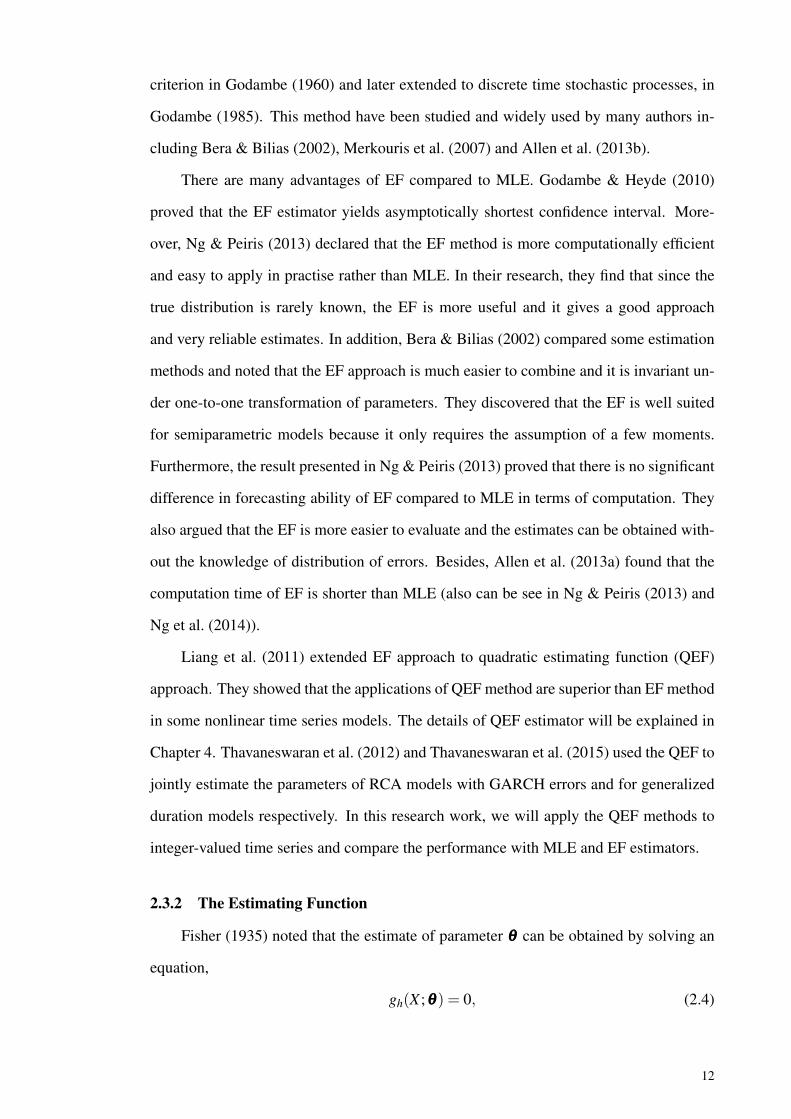
Fisher (1935) noted that the estimate of parameter θθθ can be obtained by solving an
equation,
gh(X ;θθθ) = 0, (2.4)
12

where gh(X ;θθθ) is a function of the observation vector XXX = (Xt , t = 1,2, . . . ,n) and param-
eter θθθ . The classic approach of estimation required conditions on the resulting estimator
θθθ , such as unbiasedness, consistency, invariance and minimum variance. But, EF has a
different approach. Instead of looking at the properties of estimator θθθ , it is more con-
cerned on the properties of EF itself. For instance, we will think about an unbiased EF
rather than an unbiased θθθ , i.e, we need
E [gh(X ;θθθ)] = 0. (2.5)
The significant role of unbiasedness and sufficiency were discussed in detail by Kimball
et al. (1946). Another criterion of a good estimator is optimality. Durbin (1960) said that,
"it seems reasonable to develop the idea of unbiased estimating equation with minimum
variance". Therefore, such idea leads to the derivation of optimal linear unbiased EFs.
2.3.3 Derivation of Optimum EF
Godambe (1960) was the first person who introduced regular estimating function
(EF) that satisfies certain conditions and came up with the procedure to choose an optimal
EF. The required conditions for a function g(X ;θθθ) to be a regular EF are:
(i) E[g(X ;θθθ)] =∫
g(X ;θθθ) f (X ;θθθ)dX = 0,
(ii) dg(X ;θθθ)dθθθ exists for all θθθ ∈ ΘΘΘ, where ΘΘΘ is the parameter space,
(iii)∫
g(X ;θθθ) f (X ;θθθ)dX is differentiable under the sign of integration,
(iv) E[
dg(X ;θθθ)dθθθ
]2> 0, for all θθθ ∈ ΘΘΘ,
(v) Var[g(X ;θθθ)] = E[g2(X ;θθθ)] < ∞, where f (X ;θθθ) is the density function of extreme
value distribution.
According to Godambe (1960), to find the optimal function of EF, denoted as g∗ (X ;θθθ),
two criteria should be satisfied. First, the estimated parameter should be as close as
possible to the true value. It means that the variance, Var [g(X ;θθθ)] = E[g2 (X ;θθθ)
]should be minimized, therefore E
[g∗2 (X ;θθθ)
]≤ E
[g2 (X ;θθθ)
]where g∗ (X ;θθθ) is the op-
timal estimating functions. The second criteria is the expected value of derivatives of
function g(X ;θθθ) with respect to θθθ ,
E[
dg(X ;θθθ)dθθθ
]should be as large as possible i.e
E[
dg∗(X ;θθθ)dθθθ
]≥
E[
dg(X ;θθθ)dθθθ
]. That measure of sensitivity requirement can be ob-
13
served as an identification condition. By applying both principles, the g∗ (X ;θθθ) can be
defined.
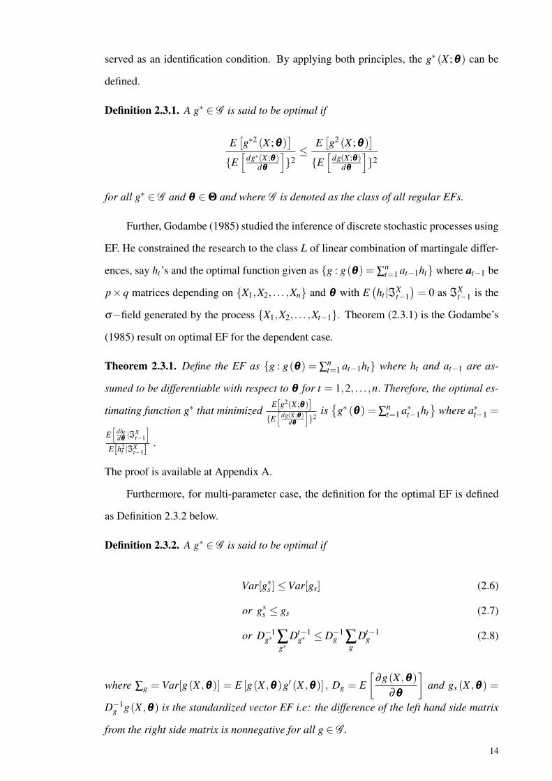
Definition 2.3.1. A g∗ ∈ G is said to be optimal if
E[g∗2 (X ;θθθ)
]E[
dg∗(X ;θθθ)dθθθ
]2
≤E[g2 (X ;θθθ)
]E[
dg(X ;θθθ)dθθθ
]2
for all g∗ ∈ G and θθθ ∈ ΘΘΘ and where G is denoted as the class of all regular EFs.
Further, Godambe (1985) studied the inference of discrete stochastic processes using
EF. He constrained the research to the class L of linear combination of martingale differ-
ences, say ht’s and the optimal function given as g : g(θθθ) = ∑nt=1 at−1ht where aaat−1 be
p× q matrices depending on X1,X2, . . . ,Xn and θθθ with E(ht |ℑX
t−1)= 0 as ℑX
t−1 is the
σ−field generated by the process X1,X2, . . . ,Xt−1. Theorem (2.3.1) is the Godambe’s
(1985) result on optimal EF for the dependent case.
Theorem 2.3.1. Define the EF as g : g(θθθ) = ∑nt=1 at−1ht where ht and at−1 are as-
sumed to be differentiable with respect to θθθ for t = 1,2, . . . ,n. Therefore, the optimal es-
timating function g∗ that minimizedE[g2(X ;θθθ)]
E[
dg(X ;θθθ)dθθθ
]2
is
g∗ (θθθ) = ∑nt=1 a∗t−1ht
where a∗t−1 =
E[
dhtdθθθ |ℑX
t−1
]E[h2
t |ℑXt−1]
.
The proof is available at Appendix A.
Furthermore, for multi-parameter case, the definition for the optimal EF is defined
as Definition 2.3.2 below.
Definition 2.3.2. A g∗ ∈ G is said to be optimal if
Var[g∗s ]≤Var[gs] (2.6)
or g∗s ≤ gs (2.7)
or D−1g∗ ∑
g∗Dt−1
g∗ ≤ D−1g ∑
gDt−1
g (2.8)
where ∑g = Var[g(X ,θθθ)] = E [g(X ,θθθ)g′ (X ,θθθ)] , Dg = E[
∂g(X ,θθθ)∂θθθ
]and gs (X ,θθθ) =
D−1g g(X ,θθθ) is the standardized vector EF i.e: the difference of the left hand side matrix
from the right side matrix is nonnegative for all g ∈ G .
14

The proof is available in Bera et al. (2006).
This method further developed onto QEF method. Such estimator was first intro-
duced by Liang et al. (2011) whereby the authors studied the quadratic martingale es-
timating functions and showed that when the conditional mean and variance of the ob-
served process depend on the same parameter of interest, then the QEF method shows
better performance compared to EF method. Furthermore, from Liang et al. (2011), the
QEF method is shown to be more informative compared to EF method by comparing
their information. The methodology proposed later has been investigated by many au-
thors including Ng et al. (2015) and Thavaneswaran et al. (2015). They showed that QEF
method give the superior results either in simulation studies or real examples in ACD
model compared to existing methods. However, the method has not been investigated to
IVTS model. For this research, we attempt to apply QEF method to estimate the parame-
ters of the IVTS models. The detail of QEF is given in Chapter 4.
15

CHAPTER 3
MOMENT PROPERTIES OF SOME INTEGER-VALUED TIME SERIESMODEL
3.1 Introduction
IVTS models are broadly applied in various fields especially biomedicine, epidemi-
ology, economics and meteorology. For example, Zeger (1988) studied the monthly cases
of Polio infection in US from 1970 to 1983, while Johansson (1996) looked at the effect
of lowering the speed limits on the number of accidents and Li et al. (2014) studied the
implication of crime cases over time. Hence, there is a strong need for IVTS models to
be studied and consequently improved further, which is the focus of this study.
Ferland et al. (2006) proposed a new integer-valued time series model as an analogue
of the generalized autoregressive conditional heteroskedastic (GARCH (p,q)) model with
Poisson as conditional distribution. This model will be explained in detail in Chapter 5.
It is later extended, for example, by Weiß (2013) in modelling time series of counts deal-
ing with overdispersion. Zhu (2011) introduced NBINGARCH(p,q) while Zhu (2012)
suggested ZIPINGARCH(p,q) model. Fokianos et al. (2009) considered geometric er-
godicity and likelihood-based inference for linear and nonlinear Poisson autoregression.
3.2 The Class of Integer-Valued GARCH Models
In this thesis, we focus on three IVTS models, namely,
(a) INGARCH(p,q):
Xt |ℑXt−1 ∼ P(λt,P)
λt,P = γ +p
∑i=1
αiXt−i +q
∑j=1
β jλt− j,P
(b) NBINGARCH(p,q):
Xt |ℑXt−1 ∼ NB(r,λt,NB)
λt,NB =1− pt
pt= γ +
p
∑i=1
αiXt−i +q
∑j=1
β jλt− j,NB
16

(c) ZIPINGARCH(p,q):
Xt |ℑXt−1 ∼ ZIP(λt,ZIP,ω)
λt,ZIP = γ +p
∑i=1
αiXt−i +q
∑j=1
β jλt− j,ZIP
where pt is the probability of successes trials, ω is the inflation parameter lies between
zeo and unity, r is the number of succeses trials, λt is the intensity parameter, ℑXt−1 is
the σ−field generated by Xt−1,Xt−2, . . . ,X1, γ > 0, αi ≥ 0, i = 1,2, . . . , p, β j ≥ 0 and
j = 1,2, . . . ,q
The above models can be written as follow:
E(Xt |ℑX
t−1)
= aλt,T P (3.1)
λt,T P = γ +p
∑i=1
αiXt−i +q
∑j=1
β jλt− j,T P (3.2)
where T P=P,NB or ZIP, a is the coefficient of the conditional mean with a= 1 and a= r
are for INGARCH and NBINGARCH models respectively while for ZIPINGARCH, it is
given as a = 1−ω with γ > 0, αi ≥ 0, i = 1,2, . . . , p and β j ≥ 0, j = 1,2, . . . ,q. Each
of these models will be explained in detail in Chapters 5-7 respectively.
3.3 First and Second Moments of The Model
The new class of models can be written in standard ARMA representation. Us-
ing martingale transformation, ut = Xt −E(Xt |ℑXt−1) = Xt − aλt,T P with E(ut) = 0 and
var(ut) = σ2u and multiplying Equation (3.2) by a gives
aλt,T P = aγ +ap
∑i=1
αiXt−i +aq
∑j=1
β jλt− j,T P.
The Equation then can be rewritten as
Xt −ut = aγ +ap
∑i=1
αiXt−i +q
∑j=1
β j(Xt− j −ut− j
)(
Xt −ap
∑i=1
αiXt−i −q
∑j=1
β jXt− j
)= aγ +ut −
q
∑j=1
β jut− j. (3.3)
Since ut is martingale difference sequence and Xt is a time series process, Equation
17
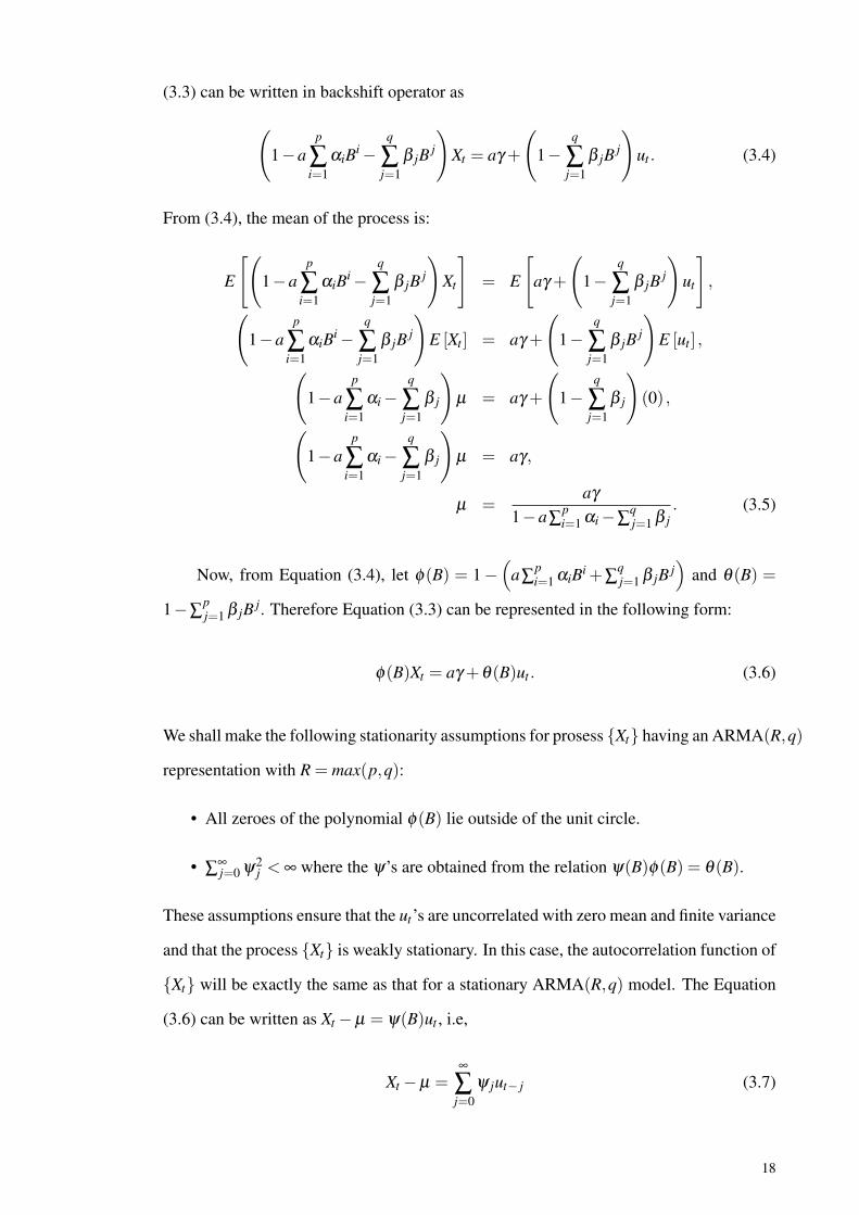
(3.3) can be written in backshift operator as
(1−a
p
∑i=1
αiBi −q
∑j=1
β jB j
)Xt = aγ +
(1−
q
∑j=1
β jB j
)ut . (3.4)
From (3.4), the mean of the process is:
E
[(1−a
p
∑i=1
αiBi −q
∑j=1
β jB j
)Xt
]= E
[aγ +
(1−
q
∑j=1
β jB j
)ut
],(
1−ap
∑i=1
αiBi −q
∑j=1
β jB j
)E [Xt ] = aγ +
(1−
q
∑j=1
β jB j
)E [ut ] ,(
1−ap
∑i=1
αi −q
∑j=1
β j
)µ = aγ +
(1−
q
∑j=1
β j
)(0) ,(
1−ap
∑i=1
αi −q
∑j=1
β j
)µ = aγ,
µ =aγ
1−a∑pi=1 αi −∑q
j=1 β j. (3.5)
Now, from Equation (3.4), let ϕ(B) = 1−(
a∑pi=1 αiBi +∑q
j=1 β jB j)
and θ(B) =
1−∑pj=1 β jB j. Therefore Equation (3.3) can be represented in the following form:
ϕ(B)Xt = aγ +θ(B)ut . (3.6)
We shall make the following stationarity assumptions for prosess Xt having an ARMA(R,q)
representation with R = max(p,q):
• All zeroes of the polynomial ϕ(B) lie outside of the unit circle.
• ∑∞j=0 ψ2
j < ∞ where the ψ’s are obtained from the relation ψ(B)ϕ(B) = θ(B).
These assumptions ensure that the ut’s are uncorrelated with zero mean and finite variance
and that the process Xt is weakly stationary. In this case, the autocorrelation function of
Xt will be exactly the same as that for a stationary ARMA(R,q) model. The Equation
(3.6) can be written as Xt −µ = ψ(B)ut , i.e,
Xt −µ =∞
∑j=0
ψ jut− j (3.7)
18

and the variance of Xt is given by
σ2X = σ2
u
∞
∑j=0
ψ2j . (3.8)
The first interest here is to derive the general formula for the first two moments,
autocovariance and autocorrelation of the integer-valued process Xt. The result is given
in Proposition 1.
Proposition 1. Under the stationarity assumption, the mean, variance, autocovariance
and autocorrelation of the the integer-valued process Xt are
(a) µX =aγ
1−a∑pi=1 αi −∑q
j=1 β j,
(b) σ2X = σ2
u
∞
∑j=0
ψ2j
(c) γXk = σ2
u
∞
∑j=0
ψ jψ j+k
(d) ρXk =
∑∞j=0 ψ jψ j+k
∑∞j=0 ψ2
j
The proof is available at Appendix C.
3.4 Skewness and Kurtosis
In the literature only the first two moments and the autovovariance are given for
integer-valued volatility models considered. In this section, following Thavaneswaran et
al. (2015), we obtain a general expression for the skewness and kurtosis for conditionally
Poisson, negative binomial and zero-inflated Poisson distributions.
Proposition 2. Under the assumption of stationarity and finite fourth moment, the process
in the form Xt −µ = ∑∞j=0 ψ jut− j where µ is the mean of the random process, ut is an
uncorrelated noise process with mean zero, variance, σ2u , skewness, Γ(u) and kurtosis,
K(u). Define St = (Xt −µ)2. Then,
(a) Var(St) =(
K(u)−3)
σ4u
∞
∑j=0
ψ4j +2σ4
u
(∞
∑j=0
ψ2j
)2
,
19

(b) Γ(X) =∑∞
j=0 ψ3j Γ(u)
(∑∞j=0 ψ2
j )3/2 ,
(c) K(X) = 3+
(K(u)−3
)∑∞
j=0 ψ4j(
∑∞j=0 ψ2
j
)2 ,
(d) ρSk =
(K(u)−2)∑∞j=0 ψ2
j ψ2j+k +2
(∑∞
j=0 ψ jψ j+k
)2
(K(u)−3)∑∞j=0 ψ4
j +2(
∑∞j=0 ψ2
j
)2 .
The proof is available at Appendix D.
3.4.1 Example on p = 1 and q = 1
From Section 3.3, the class of IVTS models considered in this study can be written
in ARMA representation as Equation (3.7) with parameter ψ j. For the case of p = 1 and
q = 1, we can find the weight of ψ j by using ϕ(B) = aα1B+ β1B and Equation (3.7),
therefore, we have
∞
∑j=1
ψ jB j =1−β1B1−ϕ(B)
. (3.9)
Using geometric series, Equation (3.9) become
∞
∑j=0
ψ jB j =
1+ϕB+ϕ 2B2 +ϕ 3B3 + . . .(1−β1B) .
Hence, the weight of ψ j is given as
ψ0 = 1,
ψ1 = ϕ −β1 = (aα1 +β1)−β1 = aα1,
ψ2 = ϕ 2 −ϕβ1 = (aα1 +β1)2 −β1 (aα1 +β1) = (aα1 +β1)(aα1 +β1 −β1)
= α1 (aα1 +β1) ,
ψ3 = ϕ 3 −ϕ 2β1 = (aα1 +β1)3 −β1 (aα1 +β1)
2 = (aα1 +β1)2 (aα1 +β1 −β1)
= α1 (aα1 +β1)2 ,
...
ψ j = α1 (aα1 +β1)j−1 . (3.10)
20

In a nutshell, it is shown that the weight ψ j = aα1 (aα1 +β1)j−1 for ψ0 = 1, for j =
1,2, . . . where a = 1, for INGARCH (1,1), a = r for NBINGARCH (1,1) and a = 1−ω
for ZIPINGARCH (1,1).
Then, using the results obtained in Equation (3.10), power summation for the weight
of ψ j are given as:
∞
∑j=0
ψ2j = 1+(aα1)
2 +(aα1 (aα1 +β1))2 + . . .+
(aα1 (aα1 +β1)
j−1)2
+ . . .
= 1+(aα1)2
1+(aα1 +β1)2 + . . .+(aα1 +β1)
2 j−2 + . . .. (3.11)
Then, we summarize Equation (3.11) giving
∞
∑j=0
ψ2j = 1+(aα1)
2
[1
1− (aα1 +β1)2
]
=1− (aα1 +β1)
2 +(aα1)2
1− (aα1 +β1)2 . (3.12)
By using the same approach finding ∑∞j=0 ψ2
j , we have
∞
∑j=0
ψ3j =
1−3α21 a2β1 −3aα1β 2
1 −β 31
1− (aα1 +β1)3 , and
∞
∑j=0
ψ4j =
1−4a3α31 β1 −6a2α2
1 β 21 −4aα1β 3
1 −β 41
1− (aα1 +β1)4 .
On the other hand, we can find ∑∞j=0 ψ jψ j+k, using the following steps.
∞
∑j=0
ψ jψ j+k =[aα1 (aα1 +β1)
k−1]+aα1
[aα1 (aα1 +β1)
k]
+aα1 (aα1 +β1)[aα1 (aα1 +β1)
k+1]
+aα1 (aα1 +β1)2[aα1 (aα1 +β1)
k+2]+ . . . ,
= aα1 (aα1 +β1)k−1 +aα1
[aα1 (aα1 +β1)
k]
+aα1
[aα1 (aα1 +β1)
k+2]
+aα1
[aα1 (aα1 +β1)
k+4]+ . . . . (3.13)
21

Equation (3.13) can be summarized as
∞
∑j=0
ψ jψ j+k = aα1 (aα1 +β1)k−1
1+aα1 (aα1 +β1)+aα1 (aα1 +β1)
3
+aα1 (aα1 +β1)5 + . . .
,
= aα1 (aα1 +β1)k−1
1+aα1 (aα1 +β1)
1+(aα1 +β1)
2+
(aα1 +β1)4 + . . .
.
Treating the Equation using geometric series, we have:
∞
∑j=0
ψ jψ j+k = aα1 (aα1 +β1)k−1
1+aα1 (aα1 +β1)
[1
1− (aα1 +β1)2
],
= aα1 (aα1 +β1)k−1
1−aα1β1 −β 2
1
1− (aα1 +β1)2
.
(3.14)
Meanwhile, we use the same technique for ∑∞j=0 ψ2
j ψ2j+k and we obtain ∑∞
j=0 ψ2j ψ2
j+k as
below:
∞
∑j=0
ψ2j ψ2
j+k = a2α21 (aα1 +β1)
2k−2
1− (aα1 +β1)
4 +a2α21 (aα1 +β1)
2
1− (aα1 +β1)4
. (3.15)
Using Equation (3.11) and (3.14), the variance, autocovariance and autocorrelation for
the models with order p = 1 and q = 1 are given by
var (Xt) = σ2u
∞
∑j=0
ψ2j = σ2
u
[1−2aα1β1 −β 2
1
1− (aα1 +β1)2
], (3.16)
cov(XtXt+k) = σ2u
∞
∑j=0
ψ jψ j+k = σ2u aα1 (aα1 +β1)
k−1
1−aα1β1 −β 2
1
1− (aα1 +β1)2
, (3.17)
and
corr (XtXt+k) =σ2
u ∑∞j=0 ψ jψ j+k
σ2u ∑∞
j=0 ψ2j
=aα1 (aα1 +β1)
k−1 (1−aα1β1 −β 21)
1−2aα1β1 −β 21
(3.18)
22
respectively.
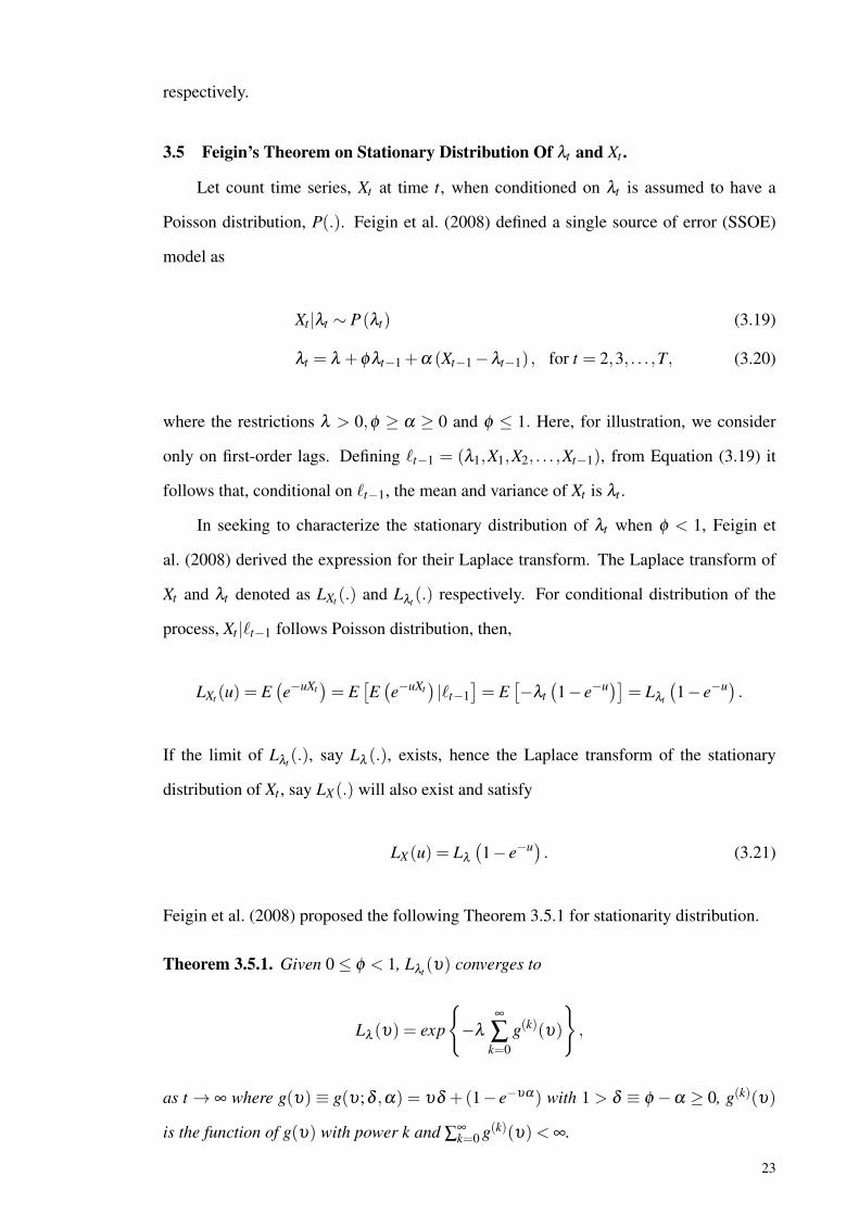
3.5 Feigin’s Theorem on Stationary Distribution Of λt and Xt .
Let count time series, Xt at time t, when conditioned on λt is assumed to have a
Poisson distribution, P(.). Feigin et al. (2008) defined a single source of error (SSOE)
model as
Xt |λt ∼ P(λt) (3.19)
λt = λ +ϕλt−1 +α (Xt−1 −λt−1) , for t = 2,3, . . . ,T, (3.20)
where the restrictions λ > 0,ϕ ≥ α ≥ 0 and ϕ ≤ 1. Here, for illustration, we consider
only on first-order lags. Defining ℓt−1 = (λ1,X1,X2, . . . ,Xt−1), from Equation (3.19) it
follows that, conditional on ℓt−1, the mean and variance of Xt is λt .
In seeking to characterize the stationary distribution of λt when ϕ < 1, Feigin et
al. (2008) derived the expression for their Laplace transform. The Laplace transform of
Xt and λt denoted as LXt (.) and Lλt (.) respectively. For conditional distribution of the
process, Xt |ℓt−1 follows Poisson distribution, then,
LXt (u) = E(e−uXt
)= E
[E(e−uXt
)|ℓt−1
]= E
[−λt
(1− e−u)]= Lλt
(1− e−u) .
If the limit of Lλt (.), say Lλ (.), exists, hence the Laplace transform of the stationary
distribution of Xt , say LX(.) will also exist and satisfy
LX(u) = Lλ(1− e−u) . (3.21)
Feigin et al. (2008) proposed the following Theorem 3.5.1 for stationarity distribution.
Theorem 3.5.1. Given 0 ≤ ϕ < 1, Lλt (υ) converges to
Lλ (υ) = exp
−λ
∞
∑k=0
g(k)(υ)
,
as t → ∞ where g(υ) ≡ g(υ ;δ ,α) = υδ +(1− e−υα) with 1 > δ ≡ ϕ −α ≥ 0, g(k)(υ)
is the function of g(υ) with power k and ∑∞k=0 g(k)(υ)< ∞.
23

The proof is available at Appendix B. Hence, under this theorem, we can conclude that,
our IVTS process are stationary as t → ∞. Using the stationarity condition, E(Xt) = µ
and for large t, E(λt) converge to λ . Using this convergence in mean, we can apply that
limt→∞E[|λt |k
]= E
[|λ |k
], where λ =
µa
.
3.6 Summary of The Chapter
In this chapter, we introduced a class of IVTS models inspired by GARCH(p,q)
model with unconditional distribution following Poisson, negative binomial and zero-
inflated Poisson namely INGARCH(p,q), NBINGARCH(p,q) or ZIPINGARCH(p,q)
models respectively. Then, we represented these models in ARMA representation and
achieved our first objective by producing general close form expressions for the first four
moments (mean, variance, skewness and kurtosis). Martingale differences were used to
simplify the derivations and for the special case of p = 1 and q = 1, the ψ j weights were
obtained explicitly. However, for the existence of first four moments, only Ferland et al.
(2006) showed the existence of moments for all order for INGARCH(p,q) model and
for the other two models, NBINGARCH(p,q) and ZIPINGARCH(p,q), their existence
of higher order of moments are still in discussion. Such existence for INGARCH(p,q)
model can be found through the additive property of its conditional distribution which
is Poisson distribution. Through such property, the process is built and its sequences are
obtained using a cascade on a random variable via a sequence of i.i.d Poisson random vari-
ables, known as thinning operation. Unfortunately, such property does not work for the
other two models, which are, NBINGARCH(p,q) and ZIPINGARCH(p,q) models. For
NBINGARCH(p,q) model, where its conditional distribution follows negative binomial
distribution, such property is applicable only on same pi’s while for ZIPINGARCH(p,q)
model, nobody have looked at the problems. In fact, neither the thinning operation in
Ferland et al. (2006) nor the coupling technique discussed in Franke (2010) in building
the model can be applied on zero-inflated cases. Therefore, since the construction can-
not be shown, its existence higher order moments also cannot be shown. To prove such
existence, a new technique should be developed and implemented where it is still under
discussion among the statisticians.
24

CHAPTER 4
THE QUADRATIC ESTIMATING FUNCTIONS
4.1 Introduction
Since the introduction by Godambe (1960), estimating functions (EF) had been ap-
plied in many areas including time series and related models (see Allen et al. (2013b),
Thavaneswaran & Abraham (1988), Li et al. (2014), Chandra & Taniguchi (2001) and
Thavaneswaran et al. (2015)). It is shown that in many studies, EF is computationally
more efficient and easy to apply in real cases compared to the traditional parameter esti-
mation, MLE.
Later, the EF method have been extended to quadratic estimating functions (QEF) by
Liang et al. (2011). In their study, it is shown that QEF methods are more informative than
the EF method when the first four conditional moments of the model are known (see Tha-
vaneswaran et al. (2012) and Thavaneswaran et al. (2015)). In addition, Thavaneswaran
et al. (2015), Liang et al. (2011), Merkouris et al. (2007) and Crowder (1987) showed that
this extension leads to improvement in terms of the efficiencies of resulting estimates.
At the same time, QEF method removes the problem of identifiability. Furthermore, ac-
cording to Thavaneswaran et al. (2015), QEF method has standard asymptotic properties
such as consistency and asymptotic normality compared to EF method. Moreover, the
result of Monte Carlo simulation study presented in Ng et al. (2015) showed that the QEF
estimators outperform the EF estimators in almost all cases in autoregressive conditional
duration (ACD) model.
Since QEF estimator has not been discussed and applied on IVTS model, in our
research work, we will focus on studying the performance of QEF method on these pro-
cesses. We will compare the results with other estimation methods. This method will be
explained in the next section.
25

4.1.1 General Model and Method
In order to use the quadratic estimating functions (QEF), it is necessary that the first
four conditional moments are known. Consider a discrete time stochastic process, Xt , t =
1,2, . . . conditonal on ℑXt−1 where ℑX
t−1 is the σ -field generated from Xt−1,Xt−2, . . . ,X1.
The first four conditional moments are
µt(θθθ) = E[Xt |ℑX
t−1], (4.1)
σ2t (θθθ) = E
[(Xt −µt(θθθ))2 |ℑX
t−1
], (4.2)
Γt(θθθ) =1
σ3t (θθθ)
E[(Xt −µt(θθθ))3 |ℑX
t−1
], (4.3)
and
κt(θθθ) =1
σ4t (θθθ)
E[(Xt −µt(θθθ))4 |ℑX
t−1
]−3, (4.4)
For the skewness and the excess kurtosis of the process Xt, we assume that such
moment properties do not contain any additional parameters. For QEF method in es-
timating the parameter of interest, θθθ based on the observations X1, . . . ,Xn, we consider
two classes of martingale differences mt(θθθ) = Xt − µt(θθθ), t = 1, . . . ,n and st(θθθ) =
m2t (θθθ)−σ2
t (θθθ), t = 1, . . . ,n. The variance and covariance of such martingale differences,
mt and st , can be described as:
⟨m⟩t = E[m2
t (θθθ)|ℑXt−1]= E
[(Xt −µt(θθθ))2|ℑX
t−1]= σ2
t (θθθ), (4.5)
⟨s⟩t = E[s2t (θθθ)|ℑX
t−1]
= E[(Xt −µt(θθθ))4 +σ4
t (θθθ)−2σ2t (θθθ)(Xt −µt(θθθ))2|ℑX
t−1],
= σ4t (θθθ)(κt(θθθ)+2), (4.6)
⟨m,s⟩t = E[mt(θθθ)st(θθθ)|ℑX
t−1]= E
[(Xt −µt(θθθ))3 −σ2
t (θθθ)(Xt −µt(θθθ))|ℑXt−1],
= σ3t (θθθ)Γt(θθθ). (4.7)
Here, skewness and the excess kurtosis are assumed to have no additional parameters.
The optimal estimating functions also can be found for each martingale difference
26

mt and st , that are
g∗M(θθθ) =n
∑t=1
E(
∂mt(θθθ)∂θθθ |ℑX
t−1
)E(m2
t |ℑXt−1) mt(θθθ) =−
n
∑t=1
∂ µt(θθθ)∂θθθ
mt(θθθ)⟨m⟩t
, and
g∗S(θθθ) =n
∑t=1
E(
∂ st(θθθ)∂θθθ |ℑX
t−1
)E(s2t |ℑX
t−1) st(θθθ) =−
n
∑t=1
∂σ2t (θθθ)
∂θθθst(θθθ)⟨s⟩t
.
Then, the corresponding information for each component of g∗M(θθθ) and g∗S(θθθ) are
IgM(θθθ) =n
∑t=1
(E[∂mt
∂θθθ |ℑXt−1])(
E[∂ mt∂θθθ |ℑX
t−1])′
E[mtm′
t |ℑXt−1] =
n
∑t=1
∂ µt(θθθ)∂θθθ
∂ µt(θθθ)∂θθθ ′
1⟨m⟩t
and
IgS(θθθ) =n
∑t=1
(E[∂ st
∂θθθ |ℑXt−1])(
E[∂ st∂θθθ |ℑ
Xt−1])′
E[sts′t |ℑX
t−1] =
n
∑t=1
∂σ2t (θθθ)
∂θθθ∂σ2
t (θθθ)∂θθθ ′
1⟨s⟩t
.
For the discrete time stochastic process, Xt, the following Theorem 4.1.1 provides the
optimal function and optimal information matrix of the QEF for the multiparameter case.
Theorem 4.1.1. For the general model in (4.1) to (4.4), in the class of all quadratic
estimating functions of the form GQ = gQ(θθθ) = ∑nt=1 (at−1mt(θθθ)+bt−1st(θθθ)),
(a) the optimal estimating functions is given by g∗Q(θθθ) = ∑nt=1(a∗t−1mt(θθθ)+b∗
t−1st(θθθ)),
where
a∗t−1 =
(1− ⟨m,s⟩2
t⟨m⟩t⟨s⟩t
)−1(−∂ µt(θθθ)
∂θθθ1
⟨m⟩t+
∂σ2t (θθθ)
∂θθθ⟨m,s⟩t
⟨m⟩t⟨s⟩t
)and
b∗t−1 =
(1− ⟨m,s⟩2
t⟨m⟩t⟨s⟩t
)−1(∂ µt(θθθ)∂θθθ
⟨m,s⟩t
⟨m⟩t⟨s⟩t− ∂σ2
t (θθθ)∂θθθ
1⟨s⟩t
);
(b) the information Ig∗Q(θθθ) is given by
Ig∗Q(θθθ) =n
∑t=1
(1− ⟨m,s⟩2
t⟨m⟩t⟨s⟩t
)−1(∂ µt(θθθ)∂θθθ
∂ µt(θθθ)∂θθθ ′
1⟨m⟩t
+∂σ2
t (θθθ)∂θθθ
∂σ2t (θθθ)
∂θθθ ′1⟨s⟩t
−(
∂ µt(θθθ)∂θθθ
∂σ2t (θθθ)
∂θθθ ′ +∂σ2
t (θθθ)∂θθθ
∂ µt(θθθ)∂θθθ ′
)⟨m,s⟩t
⟨m⟩t⟨s⟩t
);
(c) the gain in information Ig∗Q(θθθ)− Ig∗M(θθθ) is given by
n
∑t=1
(1− ⟨m,s⟩2
t⟨m⟩t⟨s⟩t
)−1(∂ µt(θθθ)∂θθθ
∂ µt(θθθ)∂θθθ ′
⟨m,s⟩2t
⟨m⟩2t ⟨s⟩t
+∂σ2
t (θθθ)∂θθθ
∂σ2t (θθθ)
∂θθθ ′1⟨s⟩t
27

−(
∂ µt(θθθ)∂θθθ
∂σ2t (θθθ)
∂θθθ ′ +∂σ2
t (θθθ)∂θθθ
∂ µt(θθθ)∂θθθ ′
)⟨m,s⟩t
⟨m⟩t⟨s⟩t
);
(d) the gain in information Ig∗Q(θθθ)− Ig∗S(θθθ) is given by
n
∑t=1
(1− ⟨m,s⟩2
t⟨m⟩t⟨s⟩t
)−1(∂ µt(θθθ)∂θθθ
∂ µt(θθθ)∂θθθ ′
1⟨m⟩t
+∂σ2
t (θθθ)∂θθθ
∂σ2t (θθθ)
∂θθθ ′⟨m,s⟩2
t
⟨m⟩t⟨s⟩t −⟨m,s⟩2t
−(
∂ µt(θθθ)∂θθθ
∂σ2t (θθθ)
∂θθθ ′ +∂σ2
t (θθθ)∂θθθ
∂ µt(θθθ)∂θθθ ′
)⟨m,s⟩t
⟨m⟩t⟨s⟩t
).
The proof is available at Appendix E
Corollary 4.1.2. When the conditional skewness γ and kurtosis κ are constants, the op-
timal QEF and associated information, based on the martingale differences mt(θθθ) =
Xt −µt(θθθ) and st(θθθ) = mt(θθθ)2 −σt(θθθ)2, are given by
g∗Q(θθθ) =(
1− γ2
κ +2
)−1 n
∑t=1
1σ3
t (θθθ)
−σt(θθθ)∂ µt(θθθ)
∂θθθ + γκ+2
∂σ2t (θθθ)∂θθθ
mt(θθθ)
+ 1κ+2
γ ∂ µt(θθθ)
∂θθθ − 1σt(θθθ)
∂σ2t (θθθ)∂θθθ
st
and
Ig∗Q(θθθ) =(
1− γ2
κ +2
)−1
Ig∗M(θθθ)+ Ig∗S(θθθ)−
γκ +2
n
∑t=1
1σ3
t (θθθ)
∂ µt(θθθ)∂θθθ
∂σ2t (θθθ)
∂θθθ ′
+
∂σ2t (θθθ)∂θθθ
∂ µt(θθθ)∂θθθ ′
.
4.2 Zero-inflated Model
In this section, to investigate theoretically the performance of QEF method com-
pared with EF method when applied on several count models, we derive the the optimal
function and information gain using EF and QEF methods by considering two types of
zero-inflated models, namely basic zero-inflated Poisson and basic zero-inflated Poisson
regression models. We compare the results based on the information gain.
28
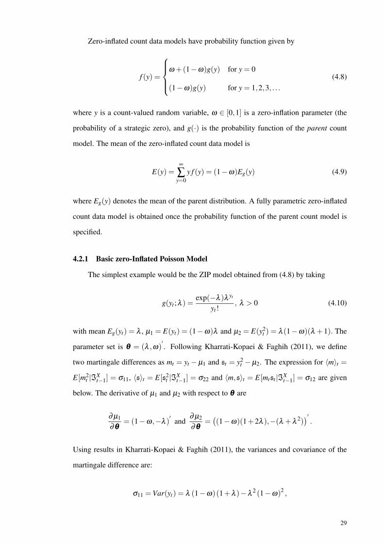
Zero-inflated count data models have probability function given by
f (y) =
ω +(1−ω)g(y) for y = 0
(1−ω)g(y) for y = 1,2,3, . . .(4.8)
where y is a count-valued random variable, ω ∈ [0,1] is a zero-inflation parameter (the
probability of a strategic zero), and g(·) is the probability function of the parent count
model. The mean of the zero-inflated count data model is
E(y) =∞
∑y=0
y f (y) = (1−ω)Eg(y) (4.9)
where Eg(y) denotes the mean of the parent distribution. A fully parametric zero-inflated
count data model is obtained once the probability function of the parent count model is
specified.
4.2.1 Basic zero-Inflated Poisson Model
The simplest example would be the ZIP model obtained from (4.8) by taking
g(yt ;λ ) =exp(−λ )λ yt
yt!, λ > 0 (4.10)
with mean Eg(yt) = λ , µ1 = E(yt) = (1−ω)λ and µ2 = E(y2t ) = λ (1−ω)(λ +1). The
parameter set is θθθ = (λ ,ω)′. Following Kharrati-Kopaei & Faghih (2011), we define
two martingale differences as mt = yt − µ1 and st = y2t − µ2. The expression for ⟨m⟩t =
E[m2t |ℑX
t−1] = σ11, ⟨s⟩t = E[s2t |ℑX
t−1] = σ22 and ⟨m,s⟩t = E[mtst |ℑXt−1] = σ12 are given
below. The derivative of µ1 and µ2 with respect to θθθ are
∂ µ1
∂θθθ= (1−ω,−λ )
′and
∂ µ2
∂θθθ=((1−ω)(1+2λ ),−(λ +λ 2)
)′.
Using results in Kharrati-Kopaei & Faghih (2011), the variances and covariance of the
martingale difference are:
σ11 =Var(yt) = λ (1−ω)(1+λ )−λ 2 (1−ω)2 ,
29

σ12 =Cov(yty2t ) = λ (1−ω)
(λ 2 +3λ +1− (1−ω)
(λ +λ 2)) , and
σ22 =Var(y2t ) = λ (1−ω)
(λ 3 +6λ 2 +7λ +1− (1−ω)λ (1+λ )2
).
Hence, using Theorem 4.1.1, the optimal QEF for each parameter are:
g∗Q(λ ) =
(1−
σ212
σ11σ22
)−1
(−1−ω
σ11+
(1−ω)(1+2λ )σ11
σ11σ22
)mt
+
((1−ω)σ12
σ11σ22+
(1−ω)(1+2λ )σ12
σ22
)st
= (1−ω)
(1
σ11σ22 −σ212
) n
∑t=1
(−σ22 +σ12(1+2λ ))mt+
(σ12 −σ11(1+2λ ))st
g∗Q(ω) =
(1−
σ212
σ11σ22
)−1[( λσ11
− (λ +λ 2)σ11
σ11σ22
)mt −
(λσ12
σ11σ22+
(λ +λ 2)σ12
σ22
)st
]= λ
(1
σ11σ22 −σ212
) n
∑t=1
((σ22 − (1+λ )σ12)mt +(σ11(1+λ )−σ12)st) .
The information matrix of the optimal θθθ is
Ig∗Q(θθθ) =
IQλλ IQ
λω
IQωλ IQ
ωω
where
IQλλ =
n(1−ω)2 (σ22 +[1+2λ ] [(1+2λ )σ11 −2σ12])
σ11σ22 −σ212
,
IQωω =
nλ 2(
σ22 +σ11 (1+λ )2 −2(1+λ )σ12
)σ11σ22 −σ2
12,
and IQωλ = IQ
λω =nλ (1−ω)
(−σ22 −σ11
(1+3λ +2λ 2)+σ12 (2+3λ )
)σ11σ22 −σ2
12.
For illustration, we compare only the information gain for parameter λ . The infor-
mation for each martingale differences, mt and st are Imλλ = n(1−ω)2/σ11 and Isλλ =
n(1−ω)2(1+ 2λ )/σ22 respectively. Therefore, we can clearly see that the value of de-
nominator of IQλλ is smaller than that Im
λλ and value of numerator is larger than that of
30

Imλλ which leads to a greater gain information for IQ
λλ compared to Imλλ and Isλλ . That is
IQλλ > Im
λλ and IQλλ > Isλλ . Similarly for IQ
ωω as well. Hence, one can say that, the combined
estimating functions are more informative than the information from each component.
4.2.2 Zero-Inflated Poisson Regression Model
In some cases, we may parameterize both λ and ω in terms of exogenous explanatory
variables, say x and z where z can be identical to x, overlap with x or completely distinct
from x. Following the definition given by Staub & Winkelmann (2013), we assume that
λ = exp(λ0 +λ1x) and ω =exp(δ0 +δ1z)
1+ exp(δ0 +δ1z). (4.11)
The parameter is θθθ = (λ0,λ1,δ0,δ1)′. The conditional expectation function of the corre-
sponding ZIP model is given by
E(y | x,z) = (1−ω)λ =exp(λ0 +λ1x)
1+ exp(δ0 +δ1z). (4.12)
Here, we consider independent counts yt , t = 1,2, . . . ,n, with parameters λt and ωt aris-
ing from Equation (4.11). Hence, the mean, variance, skewness and kurtosis of the pro-
cess are
µt(θθθ) =exp(λ0 +λ1xt)
1+ exp(δ0 +δ1zt),
σ2t (θθθ) =
exp(λ0 +λ1xt)[1+ exp(δ0 +δ1zt)+ exp(λ0 +λ1xt +δ0 +δ1zt)]
[1+ exp(δ0 +δ1zt)]2,
Γt(θθθ) =1+3λtωt +λ 2
t ωt +2λ 2t ω2
t
µt [1+λtωt ]32
, and
κt(θθθ) =ωtλ 3
t(6ω2
t −6ωt +1)+6ωtλ 2
t (2ωt −1)+7ωtλt +1
(1−ωt)λt (1+ωtλt)2 .
respectively. We take the martingale differences to be mt(θθθ) = yt − µt(θθθ) and st(θθθ) =
m2t (θθθ)−σ2
t (θθθ). The derivative of µt(θθθ) with respect to each parameter is expressed as
∂ µt(θθθ)/∂θθθ = (B1,t ,B2,t ,B3,t ,B4,t)′
where
B1,t =∂ µt(θθθ)
∂λ0=
exp(λ0 +λ1xt)
1+ exp(δ0 +δ1zt), B2,t =
∂ µt(θθθ)∂λ1
=exp(λ0 +λ1xt)xt
1+ exp(δ0 +δ1zt),
31
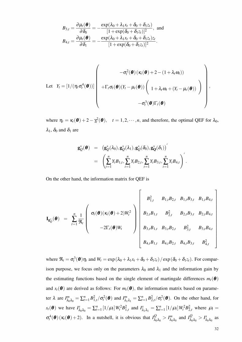
B3,t =∂ µt(θθθ)
∂δ0=−exp(λ0 +λ1xt +δ0 +δ1zt)
[1+ exp(δ0 +δ1zt)]2, and
B4,t =∂ µt(θθθ)
∂δ1=−exp(λ0 +λ1xt +δ0 +δ1zt)zt
[1+ exp(δ0 +δ1zt)]2.
Let Yt = [1/(ηtσ4t (θθθ))]
−σ2t (θθθ)(κt(θθθ)+2− (1+λtωt))
+Γtσt(θθθ)(Yt −µt(θθθ))
(1+λtωt +(Yt −µt(θθθ))
)
−σ3t (θθθ)Γt(θθθ)
,
where ηt = κt(θθθ)+ 2− γ2t (θθθ), t = 1,2, · · · ,n, and therefore, the optimal QEF for λ0,
λ1, δ0 and δ1 are
g∗Q(θθθ) =(g∗Q(λ0),g∗Q(λ1),g∗Q(δ0),g∗Q(δ1)
)′=
(n
∑t=1
YtB1,t ,n
∑t=1
YtB2,t ,n
∑t=1
YtB3,t ,n
∑t=1
YtB4,t
)′
.
On the other hand, the information matrix for QEF is
Ig∗Q(θθθ) =n
∑t=1
1ℜt
σt(θθθ)(κt(θθθ)+2)W 2
t
−2Γt(θθθ)Wt
B21,t B1,tB2,t B1,tB3,t B1,tB4,t
B2,tB1,t B22,t B2,tB3,t B2,tB4,t
B3,tB1,t B3,tB2,t B23,t B3,tB4,t
B4,tB1,t B4,tB2,t B4,tB3,t B24,t
where ℜt = σ3
t (θθθ)ηt and Wt = exp(λ0 +λ1xt +δ0 +δ1zt)/exp(δ0 +δ1zt). For compar-
ison purpose, we focus only on the parameters λ0 and λ1 and the information gain by
the estimating functions based on the single element of martingale differences mt(θθθ)
and st(θθθ) are derived as follows: For mt(θθθ), the information matrix based on parame-
ter λ are Imλ0λ0
= ∑nt=1 B2
1,t/σ2t (θθθ) and Im
λ1λ1= ∑n
t=1 B22,t/σ2
t (θθθ). On the other hand, for
st(θθθ) we have Isλ0λ0
= ∑nt=1 [1/℘t ]W 2
t B21,t and Is
λ1λ1= ∑n
t=1 [1/℘t ]W 2t B2
2,t where ℘t =
σ4t (θθθ)(κt(θθθ)+2). In a nutshell, it is obvious that IQ
λ0λ0> Im
λ0λ0and IQ
λ0λ0> Is
λ0λ0as
32

well as IQλ1λ1
> Imλ1λ1
and IQλ1λ1
> Imλ1λ1
. From the comparison, one can say that, follow-
ing the determinant optimality discussed in Bera et al. (2006), the determinant of the
combined estimating function is larger than the determinants of the information matrices
associated with the components estimating functions. That is |Ig∗Q(θθθ)| ≥ |Ig∗m(θθθ)| and
|Ig∗Q(θθθ)| ≥ |Ig∗s (θθθ)|.
4.3 Summary of The Chapter
In this chapter, we discussed the theory on QEF method proposed by Liang et al.
(2011) when applied on count data. Here, we derived the EF and QEF estimators for
two types of ZIP models namely the basic ZIP and ZIP regression. In addition, we have
also obtained closed form expressions of the information matrices for all the models and
show that the QEF with combined estimating functions is more informative than EF with
the component estimating functions. Thus, QEF method has improved the efficiency of
the estimation of parameter θθθ compared to the EF method. Hence, we can say that, the
derivation of optimal QEF function and their information matrix have shown the superi-
ority of QEF method when applied on selected zero-inflated models.
33
CHAPTER 5
INGARCH(p,q) MODEL
5.1 Introduction
Since GARCH models have given rise to new directions for research in probability
and statistics and towards developing more parsimonious models for count time series
data, Ferland et al. (2006) considered the model known as integer-valued GARCH model,
namely INGARCH(p,q) where it is a GARCH(p,q) process with Poisson conditional
distribution. He defined an INGARCH(p,q) process to be an integer-valued Xt such
that
Xt |ℑXt−1 ∼ P(λt) (5.1)
λt = γ +p
∑i=1
αiXt−i +q
∑j=1
β jλt− j (5.2)
where ℑXt−1 is the σ−field generated by Xt−1,Xt−2, . . . ,X1, γ > 0, αi ≥ 0, i = 1,2, . . . , p,
and β j ≥ 0, j = 1,2, . . . ,q.
From the definition of INGARCH(p,q) model, it is clear that INGARCH (p,0)
model actually an INARCH(p) process. It should be noted that the second-order sta-
tionarity of the process is satisfied if and only if the summation of parameter lies within
zero and one, whereby 0 < ∑pi=1 αi +∑q
j=1 β j < 1.
This model is originally proposed to model the number of cases of campylobactero-
sis infections from January 1990 to the end of October 2000 in the north of the Province
of Quèbec in Ferland et al. (2006). In this chapter, we will further study this model to
explore its moment properties by using martingale transformation of the model.
5.2 The Moment Properties
The first objective of our study is finding the moment properties of unconditional
distribution for all three models. The derivation of this unconditional moments need the
conditional moment properties. Therefore, in this section, the moments for both uncondi-
tional and conditional distribution of INGARCH(p,q) model will be derived up to order
34

four.
5.2.1 The Moment Properties of Conditional Distribution of INGARCH(p,q) Model
In INGARCH(p,q) set up, the conditional distribution of Xt given ℑXt−1 follows
Poisson. To simplify, let Yt = Xt |ℑXt−1 follows the Poisson distribution with parame-
ter λt , denoted as Yt ∼ P(λt). The moment properties of Poisson model can be ob-
tained via its probability generating function (pgf) which is G(z) = exp [λt(z−1)]. We
can get the moments of the model by finding its derivatives with evaluated at z = 1.
The first three derivatives of such pgf are G′(z) = d(exp(λt [z−1]))dz = λte(λt [z−1]), G′′(z) =
dλt(e(λt [z−1]))dz = λ 2
t e(λt [z−1]) and G′′′(z) = dλ 2t (e
(λt [z−1]))dz = λ 3
t e(λt [z−1]) respectively. In gen-
eral, we can show that, for the kth derivative, the pgf of Poisson distribution is in the form
of Gk(z) = λ kt eλt(z−1).
The mean of Poisson is given as µt = G′(1) = E(yt) = λt . The second derivative
is G′′(1) = E(yt(yt − 1)) = λ 2t . By expanding that, we will get E
(y2
t)−E (yt) = λ 2
t .
Rearrange it, then, E(y2
t)= λ 2
t + λt . The variance of Poisson distribution is σ2y,t =
E(y2
t)− E (yt)
2 = λ 2t + λt − λ 2
t = λt . For the third derivative is G′′′(1) = E(yt(yt −
1)(yt − 2)) = λ 3t . This derivative can be expanded as E
(y3
t −3y2t +2yt
)= λ 3
t . There-
fore, E(y3
t)= λ 3
t +3λ 2t +λt . Using this result, the third moment is
E[(yt −λt)
3]
= E(y3
t −3y2t λt +3ytλ 2
t −λ 3t),
= E(y3
t)−3E
(y2
t)
λt +3E (yt)λ 2t −λ 3
t ,
= λ 3t +3λ 2
t +λt −3λ 3t −3λ 2
t +3λ 3t −λ 3
t ,
= λt . (5.3)
Using Equation (D.5) in Appendix D, (5.3) and σ2y , the skewness is obtained in the fol-
lowing form:
Γ(P)t =
E[(yt −µ)3
](var(yt))
3/2 ,
=λt
λ 3/2t
,
=1√λt. (5.4)
35

Now, we find the kurtosis of Poisson distribution. The fourth derivatives of the pgf
is G′′′′(1) = E (yt (yt −1)(yt −2)(yt −3)) = λ 4t . Again, we expand the factorization to
obtain E(y4
t)
whereby E(y4
t −6y3t +11y2
t −6yt)= λ 4
t and will lead to E(y4
t)= λ 4
t +
6λ 3t +7λ 2
t +λt . Therefore, the fourth moment is
E[(yt −λt)
4]
= E(y4
t −4y3t λt +6λ 2
t y2t −4ytλ 3
t −λ 4t),
= E(y4
t)−4E
(y3
t)
λt +6λ 2t E(y2
t)−4E (yt)λ 3
t −λ 4t ,
= λ 4t +6λ 3
t +7λ 2t +λt −4λt
(λ 3
t +3λ 2t +λt
)+6λ 2
t(λ 2
t +λt)−4λ 3
t λt +λ 4t ,
= λ 4t +6λ 3
t +7λ 2t +λt −4λ 4
t −12λ 3t −4λ 2
t +6λ 4t +6λ 3
t −4λ 4t +λ 4
t ,
= 3λ 2t +λt . (5.5)
Using (D.2) in Appendix D, σ2y and Equation (5.5), the kurtosis of Poisson is
K(P)t =
E[(yt −λt)
4]
σ4y
,
=3λ 2
t +λt
λ 2t
,
= 3+1λt. (5.6)
5.2.2 The Moment Properties of Unconditional Distribution of INGARCH(p,q)Model
Using the martingale difference, ut and the results in section 3.3, we obtain the mean
as µ = σ2u = E (λt) . For large t, σ2
u = λ = µ and using Theorem 3.3.1 (b), the variance
of INGARCH(p,q) model become
σ2X = µ
∞
∑j=0
ψ2j .
Now, we find the skewness and kurtosis of INGARCH(p,q) model. We first have to find
the skewness and kurtosis of the martingale difference, Γ(u) and K(u) respectively. For the
skewness of ut , we have
Γ(u) =E(u3
t)
E(u2
t)3/2
36
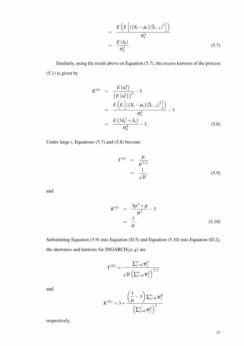
=E(
E[(Xt −µt|ℑt−1)
3])
σ3u
=E (λt)
σ3u
. (5.7)
Similarly, using the result above on Equation (5.7), the excess kurtosis of the process
(5.1) is given by
K(u) =E(u4
t)
E(u2
t)2 −3
=E(
E[(Xt −µt|ℑt−1)
2])
σ4u
−3
=E(3λ 2
t +λt)
σ4u
−3. (5.8)
Under large t, Equations (5.7) and (5.8) become
Γ(u) =µ
µ3/2
=1
õ, (5.9)
and
K(u) =3µ2 +µ
µ2 −3
=1µ. (5.10)
Substituting Equation (5.9) into Equation (D.5) and Equation (5.10) into Equation (D.2),
the skewness and kurtosis for INGARCH(p,q) are
Γ(X) =∑∞
j=0 ψ3j
õ(
∑∞j=0 ψ2
j
)3/2
and
K(X) = 3+
(1µ−3)
∑∞j=0 ψ4
j(∑∞
j=0 ψ2j
)2
respectively.
37

Ferland et al. (2006) showed the moment properties of unconditional INGARCH(p,q)
distribution only for p = 1 and q = 1 case. It should also be noted that, with our finding,
we are able to find this moments up to order four for all cases of p and q.
5.2.3 Empirical Study
To demonstrate the moments structure are correctly derived, we do the empirical
study for the cases when the process is close and far from the boundary of stationarity.
Here, we generate 500 samples of size 2000 and calculate the mean and the mean square
error of the estimated moments as tabulated in Table 5.1. It can be seen that the estimated
values are close to the true values.
Table 5.1: Generated data and true values for the moment structures with γ = 0.1
α1 = 0.1 α1 = 0.5
Estimated True MSE Estimated True MSE
β = 0.2
µX 0.9012 0.9018 8.85E-06 1.028 1.027 1.14E-05
σX2 0.9158 0.9162 3.58E-04 1.1158 1.1162 4.12E-04
Γ(X) 1.258 1.262 1.88E-04 1.052 1.059 9.48E-05
K(X) 4.125 4.108 5.22E-03 4.123 4.215 1.21E-04
β = 0.4
µX 0.7581 0.7588 1.26E-05 1.125 1.129 1.25E-05
σX2 0.9147 0.9158 1.28E-04 1.088 1.093 4.12E-04
Γ(X) 1.228 1.305 1.06E-03 1.235 1.244 1.21E-03
K(X) 4.113 4.212 4.12E-04 4.215 4.198 7.53E-04
5.3 Quadratic Estimating Functions on INGARCH(p,q) Model
In this section, we derive the optimal quadratic estimating functions, g∗Q(θθθ) for
INGARCH(p,q) model as described in Section 4.1.1.
In order to extract the g∗Q(θθθ), the first four conditional moments of INGARCH(p,q)
should be known. From Section 5.2.1, we obtained the first four conditional moments
µt(θθθ) = λt (θθθ) , (5.11)
38

σ2t (θθθ) = λt (θθθ) , (5.12)
Γt(θθθ) =1√
λt (θθθ), (5.13)
and
κt(θθθ) =1
λt (θθθ)(5.14)
where θθθ = γ,α1, . . . ,αp,β1, . . . ,βq.
In QEF method, we use two martingale differences, namely mt and st . They are
defined as mt (θθθ) = Xt −λt (θθθ) and for st (θθθ) = m2t (θθθ)−λt (θθθ) for t = 1,2, . . . ,n. The
variances and covariance of such martingale differences are
⟨m⟩t = E[m2
t (θθθ) |ℑXt−1]
= σ2t (θθθ) ,
= λt (θθθ) , (5.15)
⟨s⟩t = σ4t (θθθ)(κt (θθθ)+2) ,
= λ 2t (θθθ)
(1
λt (θθθ)+2),
= λ 2t (θθθ)
(1+2λt (θθθ)
λt (θθθ)
),
= λt (θθθ)(1+2λt (θθθ)) , (5.16)
and
⟨m,s⟩t = σ4t (θθθ)Γt (θθθ) ,
= λ 3/2t (θθθ)
1λt (θθθ)
,
= λ 1/2t (θθθ) . (5.17)
Next, we find the partial derivatives ∂ µt(θθθ)∂θ and ∂σ2
t (θθθ)∂θ . Since the conditional mean,
µt and conditional variance, σ2t are the same, we have
∂ µt (θθθ)∂θ
=∂σ2
t (θθθ)∂θ
=∂λt (θθθ)
∂θ.
39

The partial derivative of λt (θθθ) with respect to parameter θθθ are given as:
λ ′t (θθθ) =
(∂λt(θθθ)
∂γ,∂λt(θθθ)
∂α1, . . . ,
∂λt(θθθ)∂αp
,∂λt(θθθ)
∂β1, . . . ,
∂λt(θθθ)∂βq
)′
=
(1+
q
∑j=1
β j∂λt− j(θθθ)
∂γ,Xt−i +
q
∑j=1
β j∂λt− j(θθθ)
∂αi,λt− j +
p
∑k=1
βk∂λt−k(θθθ)
∂β j,
)′
,
where i = 1,2, . . . , p and j = 1,2, . . . ,q.
From Theorem 4.1.1 (a), the optimal estimation function can be achieved by finding
a∗t−1 and b∗t−1. Since
(1− ⟨m,s⟩2
t⟨m⟩t⟨s⟩t
)−1
=
(1− λ 2
t (θθθ)λ 2
t (θθθ)(1+2λt(θθθ))
)−1
,
=1+2λt(θθθ)
2λt(θθθ),
we have
a∗t−1 =
(1− ⟨m,s⟩2
t⟨m⟩t⟨s⟩t
)−1(−∂ µt(θθθ)
∂θθθ1
⟨m⟩t+
∂σ2t (θθθ)
∂θθθ⟨m,s⟩t
⟨m⟩t⟨s⟩t
),
=1+2λt(θθθ)
2λt(θθθ)
[−λt ′(θθθ)
1λt(θθθ)
+λt ′(θθθ)λt(θθθ)
(1+2λt(θθθ))λ 2t (θθθ)
],
=−λt ′(θθθ)
λt(θθθ),
and
b∗t−1 =
(1− ⟨m,s⟩2
t⟨m⟩t⟨s⟩t
)−1(∂ µt(θθθ)∂θθθ
⟨m,s⟩t
⟨m⟩t⟨s⟩t− ∂σ2
t (θθθ)∂θθθ
1⟨s⟩t
),
=1+2λt(θθθ)
2λt(θθθ)
[λt ′(θθθ)
(1
λt(θθθ)(1+2λt(θθθ))
)−λt ′(θθθ)
(1
λt(θθθ)(1+2λt(θθθ))
)],
= 0.
Since b∗t−1 is zero, we can say that, for INGARCH(p,q), the QEF estimator reduces to
EF estimator. Hence, the optimal estimating functions for each parameter are:
g∗Q(γ) =n
∑t=1
1γ +∑p
i=1 αiXt−i +∑qj=1 β jλt− j(θθθ)
40

[1+
q
∑j=1
β j∂λt− j(θθθ)
∂γ
](Xt −γ +
p
∑i=1
αiXt−i +q
∑j=1
β jλt− j(θθθ)
),
(5.18)
g∗Q(αi) =n
∑t=1
1γ +∑p
i=1 αiXt−i +∑qj=1 β jλt− j(θθθ)
[Xt−i +
q
∑j=1
β j∂λt− j(θθθ)
∂αi
](Xt −γ +
p
∑i=1
αiXt−i +q
∑j=1
β jλt− j(θθθ)
),and
(5.19)
g∗Q(β j) =n
∑t=1
1γ +∑p
i=1 αiXt−i +∑qj=1 β jλt− j(θθθ)
[λt− j +
p
∑k=1
βk∂λt−k(θθθ)
∂β j
](Xt −γ +
p
∑i=1
αiXt−i +q
∑k=1
βkλt−k(θθθ)
),
(5.20)
for i = 1,2. . . . , p and j = 1,2, . . . ,q.
On the other hand, using Theorem 4.1.1(b), the information for the optimal QEF can
be obtained by
Ig∗Q(θθθ) =n
∑t=1
(1− ⟨m,s⟩2
t⟨m⟩t⟨s⟩t
)−1(∂ µt(θθθ)∂θθθ
∂ µt(θθθ)∂θθθ ′
1⟨m⟩t
+∂σ2
t (θθθ)∂θθθ
∂σ2t (θθθ)
∂θθθ ′1⟨s⟩t
−(
∂ µt(θθθ)∂θθθ
∂σ2t (θθθ)
∂θθθ ′ +∂σ2
t (θθθ)∂θθθ
∂ µt(θθθ)∂θθθ ′
)⟨m,s⟩t
⟨m⟩t⟨s⟩t
)=
1+2λt
2λt
∂λt
∂θθθ∂λt
∂θθθ ′
(1λt
+1
λt (1+2λt)−2
λt
λ 2t (1+2λt)
)=
1λt
∂λt
∂θθθ∂λt
∂θθθ ′ .
Let M1,t =∂λt(θθθ)
∂γ, M2,i,t =
∂λt(θθθ)∂αi,t
for i = 1,2, . . . , p and M3, j,t =∂λt(θθθ)∂β j,t
for j =
1,2, . . . ,q or can be written as:
∂ µt
∂θ=
∂σ2t
∂θ=
(∂λt(θθθ)
∂γ,∂λt(θθθ)∂α1,t
, . . . ,∂λt(θθθ)
∂αp,∂λt(θθθ)
∂β j. . . ,
∂λt(θθθ)∂βq
)′
=(M1,t ,M2,i,t , . . . ,M2,p,t ,M3, j,t , . . . ,M3,q,t
)′,
and Nt =1λt, therefore, the information matrix of the optimal quadratic estimating func-
41
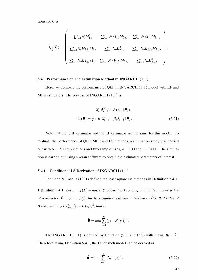
tions for θθθ is
Ig∗Q(θθθ) =
∑nt=1 NtM2
1,t ∑nt=1 NtM1,tM2,i,t ∑n
t=1 NtM1,tM3, j,t
∑nt=1 NtM2,i,tM1,t ∑n
t=1 NtM22,i,t ∑n
t=1 NtM2,i,tM3, j,t
∑nt=1 NtM3, j,tM1,t ∑n
t=1 NtM3, j,tM2,i,t ∑nt=1 NtM2
3, j,t
.
5.4 Performance of The Estimation Method in INGARCH (1,1)
Here, we compare the performance of QEF in INGARCH (1,1) model with EF and
MLE estimators. The process of INGARCH (1,1) is :
Xt |ℑXt−1 ∼ P(λt ((θθθ)) ,
λt(θθθ) = γ +α1Xt−1 +β1λt−1 (θθθ) . (5.21)
Note that the QEF estimator and the EF estimator are the same for this model. To
evaluate the performance of QEF, MLE and LS methods, a simulation study was carried
out with N = 500 replications and two sample sizes, n = 100 and n = 2000. The simula-
tion is carried out using R-cran software to obtain the estimated parameters of interest.
5.4.1 Conditional LS Derivation of INGARCH (1,1)
Lehmann & Casella (1991) defined the least square estimator as in Definition 5.4.1
Definition 5.4.1. Let Y = f (X)+noise. Suppose f is known up to a finite number p ≤ n
of parameters θθθ = (θ1, ...,θp), the least squares estimator, denoted by θθθ is that value of
θ that minimizes ∑ni=1 (yi −E (yi))
2, that is
θθθ = minn
∑i=1
(yi −E (yi))2 .
The INGARCH (1,1) is defined by Equation (5.1) and (5.2) with mean, µt = λt .
Therefore, using Definition 5.4.1, the LS of such model can be derived as
θθθ = minn
∑i=1
(Xt −µ)2 . (5.22)
42

We minimize the Equation above to obtain the value of estimated parameters via simula-
tion in R-cran software using nlminb command.
5.4.2 MLE Derivation of INGARCH (1,1)
The most well-known and traditional parameter estimation is MLE estimator. Ac-
cording to Casella & Berger (2002), MLE can be defines as in Definition (5.4.2)
Definition 5.4.2. Let X1,X2, . . . ,Xn be a random sample from distribution that depends on
one or more unknown parameters θ1,θ2, . . . ,θn with probability mass or density function
(pdf/pmf) f (θ1,θ2, . . . ,θn). Suppose that θ1,θ2, . . . ,θn is restricted to a given parameter
space Ω. Then, the maximum likelihood estimator for θi for i = 1,2, . . . ,n is
θθθ = argθ max L(θθθ , xxx) = argθ L (θθθ , xxx) ,
where L(θ1,θ2, . . . ,θn,xxx) = ∏ni=1 f (xi;θ1,θ2, . . . ,θn) and max L(θθθ , xxx)= L (θθθ , xxx).
Therefore, from Definition 5.4.2, to obtain the value of estimated parameter using
MLE, we have to maximize the loglikelihood of the model. Using Equation (5.1) and
(5.2), the loglikelihood of INGARCH (1,1) is
maxLikelihood = L =n
∑t=1
−λt +Xt ln λt − ln (Xt!) . (5.23)
We minimize the negative likelihood using nlminb command in R-cran software in order
to estimate the parameters of interest.
5.4.3 QEF of INGARCH (1,1)
From Section 5.3, we derive the QEF method for INGARCH(p,q) model. Using
such derivation via Equation (5.19)-(5.20), we can simply find the optimal functions for
INGARCH (1,1) as follow:
g∗Q(γ) =n
∑t=1
1γ +α1Xt−1 +β1λt−1(θθθ)
43

[1+β1
∂λt−1(θθθ)∂γ
](Xt −γ +α1Xt−1 +β1λt−1(θθθ)) ,
(5.24)
g∗Q(αi) =n
∑t=1
1γ +α1Xt−1 +β1λt−1(θθθ)
[Xt−i +β1
∂λt−1(θθθ)∂α1
](Xt −γ +α1Xt−1 +β1λt−1(θθθ)) ,and
(5.25)
g∗Q(β j) =n
∑t=1
1γ +α1Xt−1 +β1λt−1(θθθ)
[λt−1 +β1
∂λt−1(θθθ)∂β1
](Xt −γ +α1Xt−1 +β1λt−1(θθθ)) .
(5.26)
By letting g∗Q(θθθ) = 0, the simultaneous Equations can be solved using R-cran soft-
ware to give the QEF estimate of the parameters.
5.4.4 Simulation Study
Here, we discuss the steps to estimate parameters for INGARCH(1,1) model using
LS, MLE and EF/QEF methods:
• Step 1- Generate the data: We first generate the data for a given parameter vector
(γ,α1,β1) of size n = 100. We choose 10 parameter vectors which are closed to boundary
and also not close to boundary. The parameter vectors are: (0.2,0.4,0.1), (0.1,0.6,0.3),
(0.3,0.4,0.2), (0.1,0.7,0.2), (0.4,0.3,0.6), (0.2,0.8,0.1), (0.3,0.1,0.8), (0.1,0.2,0.3),
(0.3,0.1,0.4) and (0.5,0.2,0.3).
• Step 2: Initialize Parameters: Following Wurtz et al. (2009), in the second step, we set
the initial values for α1 = 0.1 and β1 = 0.8 On the other hand, we take the value of γ to be
the mean of generated data in step 1, µXt =γ
1−α1 −β1, namely, γ = 0.1µXt , (see Ferland
et al. (2006)). The choice of initial values does not influence the final estimates. It only
impact on the computational time.
• Step 3- Parameter estimation: The estimated values of γ ,α1 and β1 can be obtained as
follows:
44

⋄ For LS and MLE methods, we use command in R-cran to minimize the Equation
(5.22) and negative likelihood in Equation (5.23).
⋄ For QEF method, we solve the simultaneous optimal Equations (5.25)-(5.26) using
command in R-cran.
• Step 4- Replication: Step 1- Step 3 are repeated N = 500 times and compute the empir-
ical mean, bias, standard error and mean square error for each parameter.
These steps are repeated for series of length n = 1500 and n = 2000.
5.4.5 The Result
The performance is measured based on mean, bias, standard error(SE) and mean
squared error (MSE) for each parameters in LS, MLE and QEF estimators as shown in
Table 5.2-5.11.
Discussion
The simulation results are shown in Tables 5.2-5.11. A number of interesting results
can be highlighted. Firstly, for the set of parameters in stationarity cases, Table 5.2-5.6,
the QEF method is comparable with MLE method and outperforms LS method such that
smaller values of biasness, SE and MSE are observed for QEF. Secondly, when the data
are close to non-stationarity cases, that is when α1 + β1 approaches unity, we can see
from Table 5.7-5.11, QEF is clearly superior than MLE and LS in some the measures
especially their SE. Thirdly, as n increases from small sample size, n = 100 to large
sample sizesm n = 1500 and n = 2000, the results show that there is a decrease in the
values of the biasness, standard errors and mean square standard error for all parameters
for QEF method as shown in all tables. Hence, we can conclude that QEF method perform
well compared to LS and MLE methods in this IVTS model.
45

Tabl
e5.
2:Si
mul
atio
nre
sults
forI
NG
AR
CH(1,1)
with
γ=
0.1,
α 1=
0.2,
and
β 1=
0.3
n=10
0n=
1500
n=20
00
ML
EL
SQ
EF
ML
EL
SQ
EF
ML
EL
SQ
EF
γ
Mea
n0.
146
0.14
90.
144
0.06
80.
074
0.07
70.
072
0.07
20.
090
Bia
s0.
046
0.04
90.
044
0.03
20.
026
0.02
30.
033
0.02
80.
010
SE0.
058
0.06
20.
055
0.02
10.
022
0.01
90.
017
0.01
70.
013
MSE
9.12
E-0
32.
11E
-02
8.58
E-0
31.
38E
-03
1.95
E-0
31.
39E
-03
9.06
E-0
41.
20E
-03
9.08
e-04
α 1
Mea
n0.
102
0.10
20.
108
0.14
70.
143
0.14
80.
136
0.14
20.
186
Bia
s0.
098
0.09
80.
092
0.05
30.
057
0.05
20.
064
0.05
80.
014
SE0.
071
0.07
90.
068
0.02
10.
029
0.02
00.
012
0.02
50.
012
MSE
1.11
E-0
21.
52E
-02
1.15
E-0
25.
98E
-03
6.40
E-0
35.
99E
-03
2.29
E-0
34.
76E
-03
2.30
e-03
β 1
Mea
n0.
342
0.34
80.
343
0.32
20.
319
0.31
90.
328
0.32
00.
307
Bia
s0.
042
0.04
80.
043
0.02
20.
019
0.01
90.
023
0.02
00.
007
SE0.
073
0.07
70.
073
0.01
30.
015
0.01
40.
010
0.01
10.
009
MSE
2.12
E-0
22.
18E
-02
2.13
E-0
25.
64E
-03
7.04
E-0
35.
86E
-03
2.01
E-0
33.
94E
-35
2.08
e-03
46

Tabl
e5.
3:Si
mul
atio
nre
sults
forI
NG
AR
CH(1,1)
with
γ=
0.2,
α 1=
0.4,
and
β 1=
0.1
n=10
0n=
1500
n=20
00
ML
EL
SQ
EF
ML
EL
SQ
EF
ML
EL
SQ
EF
γ
Mea
n0.
138
0.13
50.
139
0.15
50.
155
0.15
60.
159
0.15
60.
161
Bia
s0.
062
0.06
50.
061
0.04
50.
045
0.04
40.
041
0.04
40.
039
SE0.
041
0.04
40.
041
0.03
30.
036
0.02
90.
028
0.03
00.
021
MSE
1.21
E-0
21.
25E
-02
1.23
E-0
23.
03E
-03
3.17
E-0
32.
99E
-03
1.01
E-0
32.
12E
-03
1.03
e-03
α 1
Mea
n0.
218
0.21
30.
219
0.31
20.
309
0.31
90.
312
0.30
30.
343
Bia
s0.
182
0.18
70.
181
0.08
80.
091
0.08
10.
088
0.09
70.
057
SE0.
155
0.16
00.
156
0.04
70.
052
0.04
30.
041
0.04
80.
037
MSE
3.11
E-0
23.
18E
-02
3.12
E-0
21.
69E
-03
2.46
E-0
32.
12E
-03
1.04
E-0
31.
54E
-03
1.05
e-03
β 1
Mea
n0.
231
0.23
90.
229
0.18
70.
189
0.11
70.
120
0.11
80.
104
Bia
s0.
132
0.13
90.
129
0.08
70.
089
0.01
70.
020
0.01
80.
004
SE0.
145
0.14
80.
142
0.02
20.
049
0.02
30.
010
0.02
30.
009
MSE
3.12
E-0
23.
44E
-02
3.18
E-0
25.
19E
-03
5.46
E-0
34.
77E
-03
2.07
E-0
32.
38E
-03
2.07
e-03
47

Tabl
e5.
4:Si
mul
atio
nre
sults
forI
NG
AR
CH(1,1)
with
γ=
0.3,
α 1=
0.1,
and
β 1=
0.4
n=10
0n=
1500
n=20
00
ML
EL
SQ
EF
ML
EL
SQ
EF
ML
EL
SQ
EF
γ
Mea
n0.
218
0.21
70.
219
0.24
90.
226
0.25
00.
241
0.21
60.
281
Bia
s0.
082
0.08
30.
081
0.05
10.
074
0.05
00.
059
0.08
40.
019
SE0.
106
0.11
20.
107
0.08
10.
090
0.08
20.
072
0.08
60.
076
MSE
9.46
E-0
39.
68E
-03
9.49
E-0
32.
31E
-03
4.22
E-0
33.
31E
-03
1.55
E-0
32.
21E
-03
1.59
e-03
α 1
Mea
n0.
059
0.05
70.
061
0.07
40.
068
0.07
60.
074
0.06
80.
092
Bia
s0.
041
0.04
30.
039
0.02
60.
032
0.02
40.
026
0.03
20.
008
SE0.
156
0.15
90.
152
0.03
40.
065
0.03
60.
008
0.05
50.
009
MSE
7.65
E-0
38.
12E
-03
7.71
E-0
31.
25E
-03
4.38
E-0
31.
53E
-03
9.76
E-0
41.
23E
-03
9.82
e-04
β 1
Mea
n0.
452
0.46
80.
447
0.41
00.
455
0.40
70.
405
0.42
40.
398
Bia
s0.
052
0.06
80.
047
0.01
00.
055
0.00
70.
005
0.02
40.
002
SE0.
079
0.08
20.
077
0.01
90.
019
0.01
70.
008
0.01
80.
010
MSE
1.23
E-0
22.
13E
-02
1.28
E-0
27.
75E
-03
8.91
E-0
37.
94E
-03
2.31
E-0
36.
05E
-03
2.26
e-03
48

Tabl
e5.
5:Si
mul
atio
nre
sults
forI
NG
AR
CH(1,1)
with
γ=
0.3,
α 1=
0.4,
and
β 1=
0.2
n=10
0n=
1500
n=20
00
ML
EL
SQ
EF
ML
EL
SQ
EF
ML
EL
SQ
EF
γ
Mea
n0.
154
0.14
90.
156
0.21
20.
209
0.22
90.
211
0.20
50.
277
Bia
s0.
146
0.15
10.
144
0.08
80.
091
0.07
10.
089
0.09
50.
023
SE0.
193
0.20
10.
192
0.03
70.
041
0.03
60.
031
0.03
60.
021
MSE
5.33
E-0
35.
38E
-03
5.31
E-0
31.
05E
-03
1.42
E-0
31.
06E
-03
9.56
E-0
41.
92E
-03
9.56
e-04
α 1
Mea
n0.
315
0.31
10.
318
0.38
90.
411
0.39
10.
389
0.37
90.
398
Bia
s0.
085
0.08
90.
082
0.01
10.
011
0.00
90.
011
0.02
10.
002
SE0.
145
0.14
70.
142
0.02
80.
041
0.02
70.
025
0.03
70.
021
MSE
8.91
E-0
39.
21E
-03
8.75
E-0
32.
58E
-03
3.86
E-0
32.
27E
-03
1.04
E-0
32.
21E
-03
1.04
e-03
β 1
Mea
n0.
257
0.25
90.
251
0.22
30.
225
0.21
00.
224
0.22
80.
197
Bia
s0.
057
0.05
90.
051
0.02
30.
025
0.01
00.
024
0.02
80.
003
SE0.
142
0.14
80.
144
0.06
70.
076
0.06
60.
017
0.06
80.
012
MSE
8.12
E-0
39.
05E
-03
8.23
E-0
31.
06E
-03
1.14
E-0
31.
01E
-06
9.01
E-0
41.
19E
-03
9.21
e-04
49

Tabl
e5.
6:Si
mul
atio
nre
sults
forI
NG
AR
CH(1,1)
with
γ=
0.5,
α 1=
0.2,
and
β 1=
0.3
n=10
0n=
1500
n=20
00
ML
EL
SQ
EF
ML
EL
SQ
EF
ML
EL
SQ
EF
γ
Mea
n0.
451
0.45
30.
457
0.48
60.
484
0.48
70.
485
0.47
80.
491
Bia
s0.
049
0.04
70.
043
0.01
40.
016
0.01
30.
015
0.02
20.
009
SE0.
119
0.11
90.
116
0.09
0.09
40.
090.
069
0.07
90.
069
MSE
8.98
E-0
39.
42E
-03
9.01
E-0
34.
73E
-03
4.75
E-0
34.
11E
-03
1.38
E-0
32.
92E
-03
1.39
e-03
α 1
Mea
n0.
113
0.11
00.
115
0.14
30.
137
0.14
50.
214
0.14
10.
182
Bia
s0.
087
0.09
00.
085
0.05
70.
063
0.05
50.
014
0.05
90.
018
SE0.
087
0.09
10.
082
0.02
30.
034
0.02
20.
016
0.02
90.
015
MSE
9.85
E-0
31.
26E
-02
9.81
E-0
36.
59E
-03
8.22
E-0
36.
54E
-03
1.48
E-0
32.
85E
-03
1.50
e-03
β 1
Mea
n0.
351
0.35
80.
347
0.32
20.
319
0.31
50.
323
0.32
00.
309
Bia
s0.
051
0.05
80.
047
0.02
20.
019
0.01
50.
023
0.02
00.
009
SE0.
056
0.06
20.
055
0.01
00.
011
0.01
00.
006
0.00
90.
006
MSE
1.23
E-0
31.
38E
-03
1.18
E-0
35.
36E
-03
7.46
E-0
35.
92E
-03
1.11
E-0
33.
59E
-03
1.15
e-03
50

Tabl
e5.
7:Si
mul
atio
nre
sults
forI
NG
AR
CH(1,1)
with
γ=
0.1,
α 1=
0.6,
and
β 1=
0.3
n=10
0n=
1500
n=20
00
ML
EL
SQ
EF
ML
EL
SQ
EF
ML
EL
SQ
EF
γ
Mea
n0.
054
0.05
10.
068
0.07
90.
074
0.08
20.
077
0.06
90.
091
Bia
s0.
046
0.04
90.
032
0.02
10.
026
0.01
80.
023
0.03
10.
009
SE0.
714
0.71
50.
511
0.50
90.
514
0.01
0.50
80.
513
0.00
5
MSE
2.61
E-0
12.
70E
-01
5.55
E-0
21.
98E
-02
2.44
E-0
21.
52E
-03
9.68
E-0
21.
55E
-02
9.71
e-04
α 1
Mea
n0.
645
0.65
10.
631
0.58
20.
572
0.58
40.
582
0.58
10.
590
Bia
s0.
045
0.05
10.
031
0.01
80.
028
0.01
60.
018
0.01
90.
010
SE0.
712
0.72
30.
415
0.52
60.
538
0.02
90.
523
0.52
80.
020
MSE
4.32
E-0
24.
85E
-02
1.22
E-0
26.
49E
-02
6.92
E-0
25.
34E
-03
1.42
E-0
21.
85E
-02
1.48
e-03
β 1
Mea
n0.
219
0.21
60.
231
0.22
10.
220
0.22
50.
221
0.21
80.
290
Bia
s0.
081
0.08
40.
069
0.07
90.
080
0.07
50.
079
0.08
20.
010
SE0.
612
0.61
80.
431
0.42
80.
442
0.02
90.
425
0.43
60.
015
MSE
5.21
E-0
25.
38E
-02
9.81
E-0
34.
76E
-02
4.82
E-0
23.
45E
-03
1.57
E-0
22.
61E
-02
1.58
e-03
51

Tabl
e5.
8:Si
mul
atio
nre
sults
forI
NG
AR
CH(1,1)
with
γ=
0.1,
α 1=
0.7,
and
β 1=
0.2
n=10
0n=
1500
n=20
00
ML
EL
SQ
EF
ML
EL
SQ
EF
ML
EL
SQ
EF
γ
Mea
n0.
053
0.05
00.
068
0.07
40.
072
0.07
60.
074
0.07
10.
088
Bia
s0.
047
0.05
00.
032
0.02
60.
028
0.02
40.
026
0.02
90.
012
SE0.
811
0.81
90.
528
0.60
90.
617
0.00
90.
508
0.51
50.
002
MSE
8.92
E-0
29.
11E
-02
9.48
E-0
35.
69E
-02
6.58
E-0
25.
72E
-03
1.62
E-0
22.
41E
-02
1.68
e-03
α 1
Mea
n0.
568
0.56
50.
581
0.68
20.
681
0.68
20.
681
0.60
80.
692
Bia
s0.
132
0.13
50.
119
0.01
80.
019
0.01
80.
019
0.09
20.
008
SE0.
751
0.75
90.
544
0.43
10.
451
0.02
10.
517
0.54
40.
002
MSE
7.45
E-0
19.
86E
-01
8.13
E-0
27.
04E
-02
7.45
E-0
27.
03E
-03
5.40
E-0
27.
06E
-02
5.45
e-03
β 1
Mea
n0.
258
0.26
10.
235
0.22
00.
227
0.21
60.
226
0.22
10.
207
Bia
s0.
058
0.06
10.
035
0.02
00.
027
0.01
60.
026
0.02
10.
007
SE0.
817
0.82
50.
584
0.53
40.
558
0.03
70.
618
0.54
40.
018
MSE
9.13
E-0
19.
58E
-01
7.15
E-0
28.
47E
-02
9.53
E-0
28.
45E
-03
2.46
E-0
25.
77E
-02
2.48
e-03
52
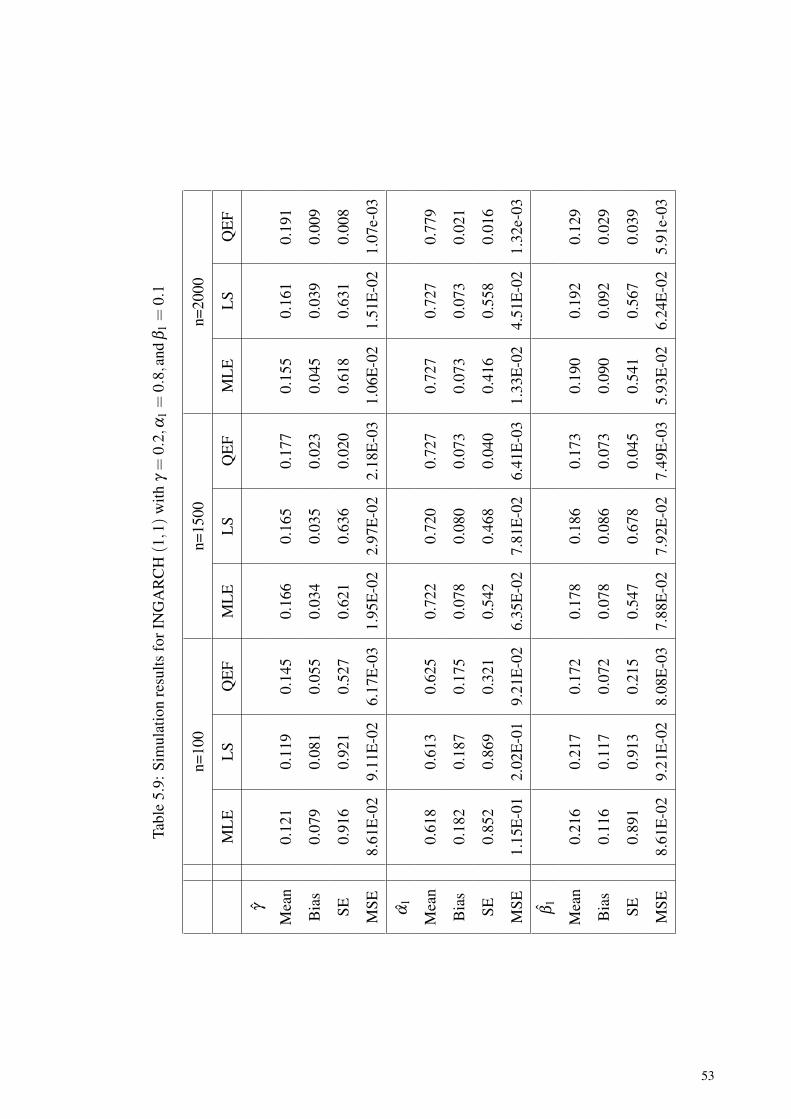
Tabl
e5.
9:Si
mul
atio
nre
sults
forI
NG
AR
CH(1,1)
with
γ=
0.2,
α 1=
0.8,
and
β 1=
0.1
n=10
0n=
1500
n=20
00
ML
EL
SQ
EF
ML
EL
SQ
EF
ML
EL
SQ
EF
γ
Mea
n0.
121
0.11
90.
145
0.16
60.
165
0.17
70.
155
0.16
10.
191
Bia
s0.
079
0.08
10.
055
0.03
40.
035
0.02
30.
045
0.03
90.
009
SE0.
916
0.92
10.
527
0.62
10.
636
0.02
00.
618
0.63
10.
008
MSE
8.61
E-0
29.
11E
-02
6.17
E-0
31.
95E
-02
2.97
E-0
22.
18E
-03
1.06
E-0
21.
51E
-02
1.07
e-03
α 1
Mea
n0.
618
0.61
30.
625
0.72
20.
720
0.72
70.
727
0.72
70.
779
Bia
s0.
182
0.18
70.
175
0.07
80.
080
0.07
30.
073
0.07
30.
021
SE0.
852
0.86
90.
321
0.54
20.
468
0.04
00.
416
0.55
80.
016
MSE
1.15
E-0
12.
02E
-01
9.21
E-0
26.
35E
-02
7.81
E-0
26.
41E
-03
1.33
E-0
24.
51E
-02
1.32
e-03
β 1
Mea
n0.
216
0.21
70.
172
0.17
80.
186
0.17
30.
190
0.19
20.
129
Bia
s0.
116
0.11
70.
072
0.07
80.
086
0.07
30.
090
0.09
20.
029
SE0.
891
0.91
30.
215
0.54
70.
678
0.04
50.
541
0.56
70.
039
MSE
8.61
E-0
29.
21E
-02
8.08
E-0
37.
88E
-02
7.92
E-0
27.
49E
-03
5.93
E-0
26.
24E
-02
5.91
e-03
53

Tabl
e5.
10:S
imul
atio
nre
sults
forI
NG
AR
CH(1,1)
with
γ=
0.3,
α 1=
0.1,
and
β 1=
0.8
n=10
0n=
1500
n=20
00
ML
EL
SQ
EF
ML
EL
SQ
EF
ML
EL
SQ
EF
γ
Mea
n0.
358
0.36
10.
355
0.33
60.
251
0.32
40.
303
0.29
10.
299
Bia
s0.
058
0.06
10.
055
0.03
60.
049
0.02
40.
003
0.00
90.
001
SE0.
517
0.53
10.
257
0.39
80.
398
0.08
40.
355
0.39
00.
057
MSE
8.62
E-0
29.
18E
-02
7.11
E-0
31.
53E
-02
1.72
E-0
21.
59E
-03
1.05
E-0
21.
55E
-02
1.02
e-03
α 1
Mea
n0.
062
0.05
90.
068
0.07
90.
074
0.08
80.
078
0.07
30.
091
Bia
s0.
038
0.04
10.
032
0.02
10.
026
0.01
10.
022
0.02
70.
009
SE0.
865
0.86
90.
258
0.61
20.
613
0.01
10.
610
0.61
00.
008
MSE
8.32
E-0
29.
18E
-02
7.88
E-0
32.
72E
-02
5.07
E-0
22.
81E
-03
1.01
E-0
23.
95E
-02
1.02
e-03
β 1
Mea
n0.
845
0.84
80.
845
0.80
90.
819
0.80
40.
822
0.82
70.
801
Bia
s0.
045
0.04
80.
045
0.00
90.
019
0.00
40.
022
0.02
70.
001
SE0.
897
0.91
60.
512
0.42
50.
430.
021
0.51
10.
526
0.00
8
MSE
9.12
E-0
29.
88E
-02
7.59
E-0
31.
72E
-02
2.32
E-0
21.
83E
-03
1.05
E-0
21.
42E
-02
1.07
e-03
54

Tabl
e5.
11:S
imul
atio
nre
sults
forI
NG
AR
CH(1,1)
with
γ=
0.4,
α 1=
0.3,
and
β 1=
0.6
n=10
0n=
1500
n=20
00
ML
EL
SQ
EF
ML
EL
SQ
EF
ML
EL
SQ
EF
γ
Mea
n0.
353
0.35
10.
379
0.38
80.
384
0.38
90.
382
0.37
80.
394
Bia
s0.
047
0.04
90.
021
0.01
20.
016
0.01
10.
018
0.02
20.
006
SE0.
187
0.19
00.
128
0.04
60.
050
0.04
80.
039
0.04
40.
035
MSE
8.92
E-0
29.
25E
-02
9.12
E-0
33.
04E
-02
3.68
E-0
22.
33E
-03
1.03
E-0
21.
98E
-02
1.03
e-03
α 1
Mea
n0.
198
0.19
20.
205
0.20
50.
218
0.22
10.
203
0.21
60.
261
Bia
s0.
102
0.10
80.
095
0.09
50.
082
0.07
90.
097
0.08
40.
039
SE0.
516
0.52
80.
214
0.01
40.
026
0.01
80.
002
0.01
50.
007
MSE
9.38
E-0
29.
87E
-02
8.26
E-0
31.
52E
-02
1.85
E-0
21.
55E
-03
1.16
E-0
21.
29E
-02
1.17
e-03
β 1
Mea
n0.
452
0.44
90.
475
0.57
40.
549
0.58
20.
589
0.57
80.
596
Bia
s0.
148
0.15
10.
125
0.02
60.
051
0.01
80.
011
0.02
20.
004
SE0.
058
0.06
20.
035
0.01
90.
021
0.01
90.
008
0.01
20.
008
MSE
7.32
E-0
27.
89E
-02
1.02
E-0
22.
19E
-02
2.47
E-0
22.
39E
-03
1.05
E-0
21.
59E
-02
1.08
e-03
55
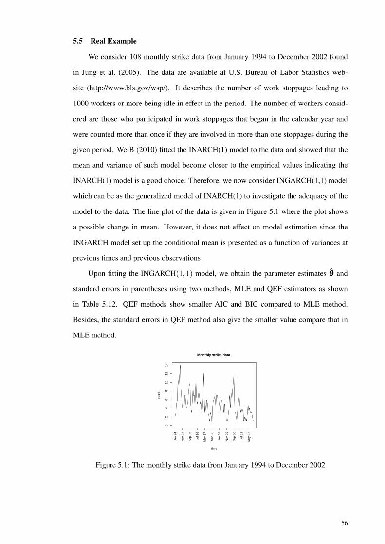
5.5 Real Example
We consider 108 monthly strike data from January 1994 to December 2002 found
in Jung et al. (2005). The data are available at U.S. Bureau of Labor Statistics web-
site (http://www.bls.gov/wsp/). It describes the number of work stoppages leading to
1000 workers or more being idle in effect in the period. The number of workers consid-
ered are those who participated in work stoppages that began in the calendar year and
were counted more than once if they are involved in more than one stoppages during the
given period. WeiB (2010) fitted the INARCH(1) model to the data and showed that the
mean and variance of such model become closer to the empirical values indicating the
INARCH(1) model is a good choice. Therefore, we now consider INGARCH(1,1) model
which can be as the generalized model of INARCH(1) to investigate the adequacy of the
model to the data. The line plot of the data is given in Figure 5.1 where the plot shows
a possible change in mean. However, it does not effect on model estimation since the
INGARCH model set up the conditional mean is presented as a function of variances at
previous times and previous observations
Upon fitting the INGARCH(1,1) model, we obtain the parameter estimates θθθ and
standard errors in parentheses using two methods, MLE and QEF estimators as shown
in Table 5.12. QEF methods show smaller AIC and BIC compared to MLE method.
Besides, the standard errors in QEF method also give the smaller value compare that in
MLE method.
02
46
810
1214
Jan
94
Nov
94
Sep
95
Jul 9
6
May
97
Mar
98
Jan
99
Nov
99
Sep
00
Jul 0
1
May
02
Monthly strike data
strik
e
time
Figure 5.1: The monthly strike data from January 1994 to December 2002
56
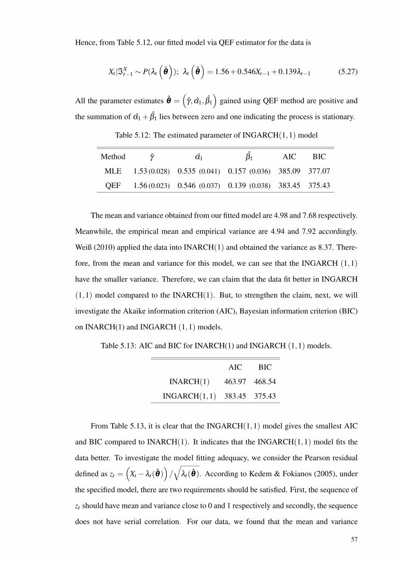
Hence, from Table 5.12, our fitted model via QEF estimator for the data is
Xt |ℑXt−1 ∼ P(λt
(θθθ)); λt
(θθθ)= 1.56+0.546Xt−1 +0.139λt−1 (5.27)
All the parameter estimates θθθ =(
γ, α1, β1
)gained using QEF method are positive and
the summation of α1 + β1 lies between zero and one indicating the process is stationary.
Table 5.12: The estimated parameter of INGARCH(1,1) model
Method γ α1 β1 AIC BIC
MLE 1.53 (0.028) 0.535 (0.041) 0.157 (0.036) 385.09 377.07
QEF 1.56 (0.023) 0.546 (0.037) 0.139 (0.038) 383.45 375.43
The mean and variance obtained from our fitted model are 4.98 and 7.68 respectively.
Meanwhile, the empirical mean and empirical variance are 4.94 and 7.92 accordingly.
Weiß (2010) applied the data into INARCH(1) and obtained the variance as 8.37. There-
fore, from the mean and variance for this model, we can see that the INGARCH (1,1)
have the smaller variance. Therefore, we can claim that the data fit better in INGARCH
(1,1) model compared to the INARCH(1). But, to strengthen the claim, next, we will
investigate the Akaike information criterion (AIC), Bayesian information criterion (BIC)
on INARCH(1) and INGARCH (1,1) models.
Table 5.13: AIC and BIC for INARCH(1) and INGARCH (1,1) models.
AIC BIC
INARCH(1) 463.97 468.54
INGARCH(1,1) 383.45 375.43
From Table 5.13, it is clear that the INGARCH(1,1) model gives the smallest AIC
and BIC compared to INARCH(1). It indicates that the INGARCH(1,1) model fits the
data better. To investigate the model fitting adequacy, we consider the Pearson residual
defined as zt =(
Xt −λt(θθθ))/
√λt(θθθ). According to Kedem & Fokianos (2005), under
the specified model, there are two requirements should be satisfied. First, the sequence of
zt should have mean and variance close to 0 and 1 respectively and secondly, the sequence
does not have serial correlation. For our data, we found that the mean and variance
57
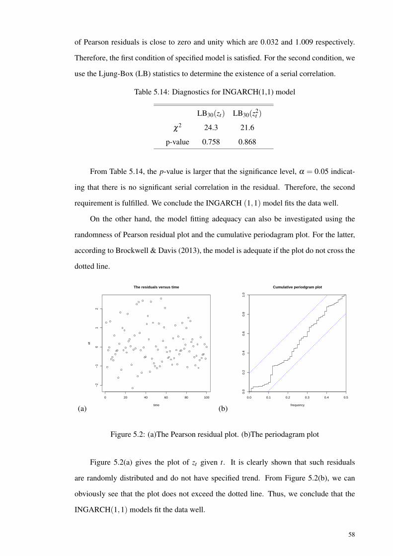
of Pearson residuals is close to zero and unity which are 0.032 and 1.009 respectively.
Therefore, the first condition of specified model is satisfied. For the second condition, we
use the Ljung-Box (LB) statistics to determine the existence of a serial correlation.
Table 5.14: Diagnostics for INGARCH(1,1) model
LB30(zt) LB30(z2t )
χ2 24.3 21.6
p-value 0.758 0.868
From Table 5.14, the p-value is larger that the significance level, α = 0.05 indicat-
ing that there is no significant serial correlation in the residual. Therefore, the second
requirement is fulfilled. We conclude the INGARCH (1,1) model fits the data well.
On the other hand, the model fitting adequacy can also be investigated using the
randomness of Pearson residual plot and the cumulative periodagram plot. For the latter,
according to Brockwell & Davis (2013), the model is adequate if the plot do not cross the
dotted line.
(a)
0 20 40 60 80 100
−2
−1
01
2
The residuals versus time
time
et
(b)
0.0 0.1 0.2 0.3 0.4 0.5
0.0
0.2
0.4
0.6
0.8
1.0
frequency
Cumulative periodgram plot
Figure 5.2: (a)The Pearson residual plot. (b)The periodagram plot
Figure 5.2(a) gives the plot of zt given t. It is clearly shown that such residuals
are randomly distributed and do not have specified trend. From Figure 5.2(b), we can
obviously see that the plot does not exceed the dotted line. Thus, we conclude that the
INGARCH(1,1) models fit the data well.
58

5.6 Summary of The Chapter
In this chapter, we focussed only on INGARCH(p,q) model. We presented a general
approach for any p and q instead of given by Ferland who gives the results only for p = 1
and q = 1. We derived the optimal QEF functions and their information matrix. To see
the performance of this method, we carried out a simulation study in which the QEF was
compared to MLE and LS. The results show that the QEF estimator is superior compared
to MLE and LS methods. Lastly, we applied the methodology on a set of real data and
showed that the INGARCH(1,1) model was a good fit and that the QEF worked well in
this case.
59

CHAPTER 6
NBINGARCH(p,q) MODEL
6.1 Introduction
Zhu (2011) highlighted that the INGARCH(p,q) model has few disadvantages. Firstly,
it does not accommodate covariates. Secondly, the ACF is always positive and lastly the
conditional distribution of INGARCH(p,q) model following Poisson, meaning that the
conditional mean and conditional variance are the same which will lead to overdispersion
Therefore, to overcome these drawbacks, Zhu (2011) proposed the same model with
negative binomial as conditional distribution which is denoted as NBINGARCH(p,q) .
The model is defined as
(Xt |ℑX
t−1)
∼ NB(r, pt) ,
1− pt
pt= λt = γ +
p
∑i=1
αiXt−i +q
∑j=1
β jλt− j. (6.1)
where γ > 0, αi ≥ 0, i= 1,2, . . . , p, j = 1,2, . . . ,q, r is the number of successes trials, ℑXt−1
is the σ−field generated from Xt−1,Xt−2, . . . ,X1 and pt is the probability of successes.
Here, as in INGARCH(p,q) model, the model satisfies the stationarity if and only if
0 < r ∑pi=1 αi +∑q
j=1 β j < 1.
6.2 The Moment Properties
In this Section, we will derive the moments of both unconditional and conditional
distribution of NBINGARCH(p,q) model up to order four.
6.2.1 The Moments of Conditional Distribution in NBINGARCH(p,q) Model
For NBINGARCH(p,q) process, the conditional distribution follows negative bino-
mial distribution. To simplify, let Yt = Xt |ℑXt−1 follows the negative binomial distribution,
Yt ∼NB(r, pt) where pt is the probability of successes. According to Johnson et al. (2005),
probability generating function (pgf) of negative binomial distribution is G(z) =(
1−qt1−qtz
)r
60

with qt = 1− pt . The first derivative can be obtained as below:
G′(z) =ddz
(1−qt
1−qtz
)r
=ddz
(1−qt)r (1−qtz)
−r
= (1−qt)r (−r)(1−qtz)
−r−1 (−qt)
= rqt (1−qt)r (1−qtz)
−r−1 . (6.2)
Using the same approach, the second and third derivatives are
G′′(z) = rq2t (1−qt)
r (r+1)(1−qtz)−r−2 ,
and
G′′′(z) = rq3t (1−qt)
r (r+1)(r+2)(1−qtz)−r−3 ,
respectively. Therefore, the k-th derivative is
Gk(z) = rqkt (1−qt)
r (r+1)(r+2) . . .(r+ k−1)(1−qtz)−r−k .
From Equation (6.2), the mean is:
µt = E(yt) = G′(1) =rqt
1−qt. (6.3)
The second derivative is
G′′(1) = E(y2
t)−E(yt) =
rq2t (r+1)
(1−qt)2 .
Rearrange it to be E(y2), therefore,
E(y2
t)=
rq2t (r+1)
(1−qt)2 +E (yt) =
rq2t (r+1)
(1−qt)2 +
rqt
1−qt=
rqt
1−qt
(rqt +11−qt
),
then, the variance for negative binomial distribution is:
var(yt) = E(y2
t)− [E(yt)]
2 ,
61
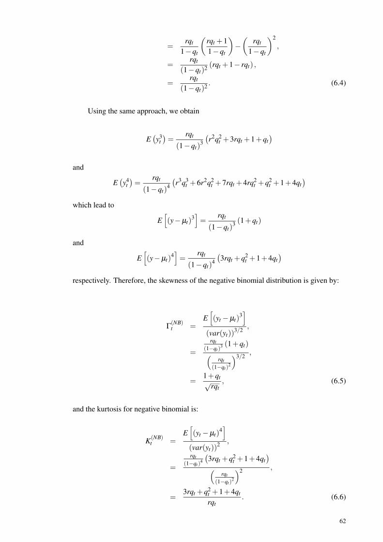
=rqt
1−qt
(rqt +11−qt
)−(
rqt
1−qt
)2
,
=rqt
(1−qt)2 (rqt +1− rqt) ,
=rqt
(1−qt)2 . (6.4)
Using the same approach, we obtain
E(y3
t)=
rqt
(1−qt)3
(r2q2
t +3rqt +1+qt)
and
E(y4
t)=
rqt
(1−qt)4
(r3q3
t +6r2q2t +7rqt +4rq2
t +q2t +1+4qt
)which lead to
E[(y−µt)
3]=
rqt
(1−qt)3 (1+qt)
and
E[(y−µt)
4]=
rqt
(1−qt)4
(3rqt +q2
t +1+4qt)
respectively. Therefore, the skewness of the negative binomial distribution is given by:
Γ(NB)t =
E[(yt −µt)
3]
(var(yt))3/2 ,
=
rqt
(1−qt)3 (1+qt)(
rqt
(1−qt)2
)3/2 ,
=1+qt√
rqt, (6.5)
and the kurtosis for negative binomial is:
K(NB)t =
E[(yt −µt)
4]
(var(yt))2 ,
=
rqt
(1−qt)4
(3rqt +q2
t +1+4qt)
(rqt
(1−qt)2
)2 ,
=3rqt +q2
t +1+4qt
rqt. (6.6)
62

We can represent the moment properties of negative binomial distribution in terms of λt
where define
λt =1− pt
pt.
Therefore, the first four moments of negative binomial distribution are:
µt = rλt , σ2t = rλt (1+λt) ,
Γ(NB) =1+2λt√
rλt (1+λt), K(NB) =
λt (1+λt)(3r+4)+2λ 2t −2λt +1
rλt (1+λt). (6.7)
6.2.2 The Moments Properties of Unconditional Distribution in NBINGARCH(p,q)Model
The mean of the NBINGARCH(p,q) is µ = E(Xt) = E[E(Xt |ℑX
t−1)]
= E [rλt ],
therefore, under large t, we have µ = rλ . The variance of the martingale difference ut
is
σ2u = E
(u2
t)= rE (λt)+ rE
(λ 2
t). (6.8)
For the skewness and kurtosis of the ut , we have
Γ(u) =E(u3
t)
E(u2
t)3/2 =
E(rλt +3rλ 2
t +2rλ 3t)[
E(rλt + rλ 2
t)]3/2 . (6.9)
Moreover, for the excess kurtosis of the model, using the same approach as skewness of
ut , Γ(u),
K(u) =E(u4
t)
E(u2
t)2 −3
=E(
E[(Xt − rλt|ℑX
t−1)2])
σ4u
−3
=E(r2λ 2
t −8rλ 2t −4rλt + r2λ 3
t −4rλ 3t)[
E(rλt + rλ 2
t)]2 . (6.10)
For large t and λ = µr , Equations (6.8), (6.9) and (6.10) become
σ2u = µ(1+
µr), (6.11)
63
Γ(u) =µ(r2 +3rµ +2µ2)
r1/2 (rµ +µ2)3/2 , and (6.12)
K(u) =µ2r2 −8µ2r−8µr2 +µ3r−4µ3
(rµ +µ)2 (6.13)
respectively.
Hence, by using Equations (6.11), (6.12) and (6.13), we can find the variance, skew-
ness and kurtosis of NBINGARCH(p,q) process which are
σ2X = µ
(1+
µr
) ∞
∑j=0
ψ2j ,
Γ(X) =µ(r2 +3rµ +2µ2)∑∞
j=0 ψ3j
r1/2 (rµ +µ2)3/2(
∑∞j=0 ψ2
j
)3/2 , and
K(X) = 3+
(µ2r2 −8µ2r−8µr2 +µ3r−4µ3)∑∞
j=0 ψ4j
(rµ +µ)2(
∑∞j=0 ψ2
j
)2
accordingly.
Zhu (2011) derived only on the mean and variance of unconditional distribution in
the NBINGARCH(p,q) model. The derivation for variance presented in Zhu’s work is
very complicated and with the order of q to be zero. Here we produced a closed form
expression for the moments up to order four for all p and q cases and the derivation is
easier to understand. This finding is very important in understanding the behavior of the
model through its higher order moment properties.
6.2.3 Empirical Study
Again, similar to Section 5.2.3, to demonstrate the moments structure are correctly
derived, we do the empirical study for the cases when the process is close and far from
the boundary of stationarity. Here, we generate 500 samples of size 2000 and fixed the
value r = 2, then, calculate the mean and the mean square error of the estimated moments
as tabulated in Table 6.1. It can be seen that the estimated values are close to the true
values.
64

Table 6.1: Generated data and true values for the moment structures with γ = 0.1
α1 = 0.1 α1 = 0.5
Estimated True MSE Estimated True MSE
β = 0.2
µX 0.8127 0.8213 7.21E-05 1.142 1.151 1.22E-04
σX2 0.8177 0.8156 1.23E-03 1.315 1.329 8.12E-03
Γ(X) 1.581 1.567 1.66E-04 1.079 1.082 5.58E-05
K(X) 4.032 4.108 4.11E-03 4.014 4.025 1.28E-05
β = 0.4
µX 0.8213 0.8236 1.44E-03 1.774 1.792 5.23E-03
σX2 0.8321 0.8344 9.12E-03 1.158 1.167 3.11E-03
Γ(X) 1.210 1.251 8.21E-03 1.582 1.596 4.53E-03
K(X) 4.234 4.247 5.14E-03 4.771 4.785 8.11E-03
6.3 Quadratic Estimating Functions on NBINGARCH(p,q) Model
The third contribution of this study is to find the optimal quadratic estimating func-
tions for each of our models. To apply the QEF in estimating the parameters of interest,
the first four conditional moments of NBINGARCH(p,q) are required and they are
µt(θθθ) = rλt (θθθ) , (6.14)
σ2t (θθθ) = rλt (θθθ)(1+λt (θθθ)) , (6.15)
Γt(θθθ) =1+2λt (θθθ)√
rλt (θθθ)(1+λt (θθθ)), (6.16)
and
κt(θθθ) =rλ 2
t (θθθ)−4λt (θθθ)−4rλt (θθθ)(1+λt (θθθ))
. (6.17)
The martingale differences of mt and st for such model are defined to be mt (θθθ) =
yt − rλt (θθθ) and st (θθθ) = m2t (θθθ)−σ2
t (θθθ) for t = 1,2, . . . ,n. Then, their variances and
covariance can be easily found as shown below:
⟨m⟩t = σ2t (θθθ) = rλt (θθθ)(1+λt (θθθ)) , (6.18)
⟨s⟩t = σ4t (θθθ)(κt(θθθ)+2) ,
65

= [rλt (θθθ)(1+λt (θθθ))]2[
rλ 2t (θθθ)−4λt (θθθ)−4
rλt (θθθ)(1+λt (θθθ))+2],
= [rλt (θθθ)(1+λt (θθθ))]2[
rλ 2t (θθθ)−4λt (θθθ)−4+2rλt (θθθ)+2rλ 2
t (θθθ)rλt (θθθ)(1+λt (θθθ))
],
= rλt (θθθ)(1+λt (θθθ))[λ 2
t (θθθ)1+2r+2λt (θθθ)r−2−4], (6.19)
and ⟨m,s⟩t = σ4t (θθθ)Γt(θθθ),
= [rλt (θθθ)(1+λt (θθθ))]3/2
[1+2λt (θθθ)√
rλt (θθθ)(1+λt (θθθ))
],
= rλt (θθθ)(1+λt (θθθ)) [1+2λt (θθθ)] . (6.20)
On the other hand, in applying the QEF estimator, we have to find the derivatives of
the mean and variance with respect to the parameter θθθ , ∂ µt(θθθ)∂θ and ∂σ2
t (θθθ)∂θ respectively
∂ µt (θθθ)∂θ
=∂ (rλt (θθθ))
∂θ= rλ ′
t (θθθ) , (6.21)
and
∂σ2t (θθθ)∂θ
=∂ [rλt (θθθ)(1+λt (θθθ))]
∂θ, (6.22)
= rλ ′t (θθθ) [1+λt (θθθ)]+λ ′
t (θθθ)rλt (θθθ) ,
= rλ ′t (θθθ) [1+2λt (θθθ)] . (6.23)
The parameters of interests are given as θθθ = (γ,α1, . . . ,αp,β1,β2, . . . ,βq)′. Therefore,
∂ µt (θθθ)∂θθθ
=
(r
∂λt (θθθ)∂γ
,r∂λt (θθθ)
∂α1. . . ,r
∂λt (θθθ)∂αp
,r∂λt (θθθ)
∂β1, . . . ,r
∂λt (θθθ)∂βq
)′
,
=(B(1,t),B(2,1,t), . . . ,B(2,p,t), . . . ,B(3,1,t), . . . ,B(3,q,t)
)′.
∂σ2t (θθθ)∂θθθ
=
(Dt
∂λt(θθθ)∂γ ,Dt
∂λt(θθθ)∂α1
, . . . ,Dt∂λt(θθθ)
∂αp,Dt
∂λt(θθθ)∂β1
, . . . ,Dt∂λt(θθθ)
∂βq,
)′
,
=(H(1,t),H(2,1,t), . . . ,H(2,p,t), . . . ,H(3,1,t), . . . ,H(3,q,t),
)′,
where Dt = r(1+ 2λt(θθθ)), B(i, j,t) is the partial derivative of the mean with respect to
each parameter and H(i, j,t) is the partial derivative of the variance with respect to each
66
parameter. In order to obtain the optimal function, we let Rt =(
1− ⟨m,s⟩2t
⟨m⟩t⟨s⟩t
)−1, Bm
k,t =
−Bk,t⟨m⟩t , Hm
k,t =Hk,t⟨m,s⟩t⟨m⟩t⟨s⟩t , T v
k,t =Bk,t⟨m,s⟩t⟨m⟩t⟨s⟩t
, and Zvk,t =
−Hk,t⟨s⟩t . Therefore, the optimal estimating
function for NBINGARCH(p,q) is given by
g∗Q(θθθ) =n
∑t=1
(a∗t−1mt +b∗
t−1st),
where
a∗t−1 = Rt
Bm(1,t)+Hm
(1,t),Bm(2,1,t)+Hm
(2,1,t), . . . ,Bm(2,p,t)+Hm
(2,p,t),
Bm(3,1,t)+Hm
(3,1,t), . . . ,Bm(3,q,t)+Hm
(3,q,t)
,
b∗t−1 = Rt
T v(1,t)+Zv
(1,t),Tv(2,1,t)+Zv
(2,1,t), . . . ,Tv(2,p,t)+Zv
(2,p,t),
T v(3,1,t)+Zv
(3,1,t), . . . ,Tv(3,q,t)+Zv
(3,q,t)
.
Thus, the optimal quadratic estimating functions for each component of θθθ are
g∗Q(γ) =n
∑t=1
Rt
[(Bm(1,t)+Hm
(1,t)
)mt +
(T v(1,t)+Zv
(1,t)
)st
],
g∗Q(αi) =n
∑t=1
Rt
[(Bm(2,i,t)+Hm
(2,i,t)
)mt +
(T v(2,i,t)+Zv
(2,i,t)
)st
], i = 1, . . . , p,
(6.24)
g∗Q(β j) =n
∑t=1
Rt
[(Bm(3, j,t)+Hm
(3, j,t)
)mt +
(T v(3, j,t)+Zv
(3, j,t)
)st
], j = 1, . . . ,q
. (6.25)
To estimate the parameters of interest, we can solve g∗Q(θθθ) using R-cran software. The
information matrix of the optimal estimating function for θθθ is given by
67

Ig∗Q(θθθ) =
IQγγ IQ
γαi IQγβ j
IQαiγ IQ
αiαi IQαiβ j
IQβ jγ IQ
β jαiIQβ jβ j
where the elements in the matrix are
IQγγ =
n
∑t=1
Rt
[B2(1,t)
⟨m⟩t+
H2(1,t)
⟨s⟩t−2B(1,t)H(1,t)
⟨m,s⟩t
⟨m⟩t⟨s⟩t
],
IQαiαi =
n
∑t=1
Rt
[B2(2,i,t)
⟨m⟩t+
H2(2,i,t)
⟨s⟩t−2B(2,i,t)H(2,i,t)
⟨m,s⟩t
⟨m⟩t⟨s⟩t
],
IQβ jβ j
=n
∑t=1
Rt
[B2(3, j,t)
⟨m⟩t+
H2(3, j,t)
⟨s⟩t−2B(3, j,t)H(3, j,t)
⟨m,s⟩t
⟨m⟩t⟨s⟩t
],
IQγαi =
n
∑t=1
Rt
[B(2,i,t)B(1,t)
⟨m⟩t+
H(2,i,t)H(1,t)
⟨s⟩t− (B(1,t)H(2,i,t)+H(1,t)B(2,i,t))
⟨m,s⟩t
⟨m⟩t⟨s⟩t
],
IQγβ j
=n
∑t=1
Rt
[B(3, j,t)B(1,t)
⟨m⟩t+
H(3, j,t)H(1,t)
⟨s⟩t− (B(1,t)H(3, j,t)+H(1,t)B(3, j,t))
⟨m,s⟩t
⟨m⟩t⟨s⟩t
]IQαiβ j
=n
∑t=1
Rt
[B(2,i,t)B(3, j,t)
⟨m⟩t+
B(2,i,t)H(3, j,t)
⟨s⟩t− (B(2,i,t)H(3, j,t)+H(2,i,t)B(3, j,t))
⟨m,s⟩t
⟨m⟩t⟨s⟩t
]
and Iαiγ = Iγαi , Iβ jγ = Iγβ j and Iβ jαi = Iαiβ j .
The optimal estimating function and associated information based on mt is given by
g∗m(θ) =−n
∑t=1
∂ µt (θθθ)∂θθθ
Xt − rλt (θθθ)
rλt (θθθ)(1+λt (θθθ))
(6.26)
and the optimal estimating function and associated information based on st is given by
g∗s (θ) =−n
∑t=1
∂σ2t (θθθ)∂θθθ
m2
t (θθθ)−σ4t (θθθ)
rλt (θθθ)(1+λt (θθθ))[λ 2
t (θθθ)1+2r+2λt (θθθ)r−2−4] .
(6.27)
We then obtain the corresponding information matrix using estimating functions based
68

on mt(θθθ) and st(θθθ) denoted as Ig∗m(θθθ) and Ig∗s (θθθ) respectively such that
Ig∗m(θθθ) =
Imγγ Im
γαiImγβ j
Imαiγ Im
αiαiImαiβ j
Imβ jγ Im
β jαiImβ jβ j
; Ig∗s (θθθ) =
Isγγ Is
γαiIsγβ j
Isαiγ Is
αiαiIsαiβ j
Isβ jγ Is
β jαiIsβ jβ j
where the elements for Ig∗m in the matrix are
Imγγ =
n
∑t=1
[B2(1,t)
⟨m⟩t
]; Im
αiαi=
n
∑t=1
[B2(2,i,t)
⟨m⟩t
]; Im
β jβ j=
n
∑t=1
[B2(3, j,t)
⟨m⟩t
];
Imγαi
=n
∑t=1
[B(2,i,t)B(1,t)
⟨m⟩t
]; Im
γβ j=
n
∑t=1
[B(3, j,t)B(1,t)
⟨m⟩t
], and Im
αiβ j=
n
∑t=1
[B(2,i,t)B(3, j,t)
⟨m⟩t
],
and the remaining elements are obtained by symmetry. The elements Ig∗s are
Isγγ =
n
∑t=1
[H2(1,t)
⟨s⟩t
]; Is
αiαi=
n
∑t=1
[H2(2,i,t)
⟨s⟩t
]; Is
β jβ j=
n
∑t=1
[H2(3, j,t)
⟨s⟩t
];
Isγαi
=n
∑t=1
[H(2,i,t)H(1,t)
⟨s⟩t
]; Is
γβ j=
n
∑t=1
[H(3, j,t)H(1,t)
⟨s⟩t
], and Is
αiβ j=
n
∑t=1
[H(2,i,t)H(3, j,t)
⟨s⟩t
].
From the information obtained using QEF and information via its components, mt(θθθ)
and st(θθθ), it is clearly seen that IQγγ > Im
γγ , IQγγ > Is
γγ , IQαiαi > Im
αiαi, IQ
αiαi > Isαiαi
, IQβ jβ j
>
Imβ jβ j
, IQβ jβ j
> Isβ jβ j
, IQγαi > Im
γγ , IQγαi > Is
γγ , IQαiβ j
> Imαiαi
, IQαiβ j
> Isαiαi
, IQαiβ j
> Imβ jβ j
,
and IQβ jβ j
> Isβ jβ j
. Based on these, we conclude that the QEF is more informative than the
component estimating functions (see Ghahramani & Thavaneswaran (2009)).
6.4 Performance of The Estimation Methods in NBINGARCH (1,1)
In this section, we compare the performance of QEF method with EF and MLE
methods in NBINGARCH (1,1) model by a simulation study with replication N = 500,
and two sample size, n = 100 and n = 2000.
NBINGARCH (1,1) process is defined as:
(Xt |ℑX
t−1)∼ NB(r, pt) ,
69
1− pt
pt= λt(θθθ) = γ +α1Xt−1 +β1λt−1. (6.28)
6.4.1 MLE Derivation of NBINGARCH (1,1)
In order to apply the MLE for the model, we first have to find loglikelihood of NBIN-
GARCH (1,1) which is
L =n
∑t=1
ln
(Xt + r−1)!(r−1)!(Xt − r)!
+ r ln
(1
1+λt
)+(Xt − r) ln
(λt
λt +1
).
To obtain the parameters of interest, we have to maximize the likelihood function using
nlminb command in R-cran.
6.4.2 EF Derivation of NBINGARCH (1,1)
The derivation of EF for NBINGARCH (1,1) can be obtained from Equation (6.26)
whereby
g∗E(θθθ) = −n
∑t=1
∂ µt (θθθ)∂θθθ
Xt − rλt (θθθ)
rλt (θθθ)(1+λt (θθθ))
,
= −n
∑t=1
rλ ′t (θθθ)
Xt − rλt (θθθ)
rλt (θθθ)(1+λt (θθθ))
,
= −n
∑t=1
λ ′t (θθθ)
Xt − rλt (θθθ)
λt (θθθ)(1+λt (θθθ))
.
Therefore, the optimal EF function for the parameters are:
g∗E(γ) = −n
∑t=1
Xt − rλt (θθθ)r
1+β1∂λt−1(θθθ)
∂γ
λt (θθθ)(1+λt (θθθ))
, (6.29)
g∗E(α1) = −n
∑t=1
Xt − rλt (θθθ)r
rXt−1 +β1∂λt−1(θθθ)
∂α1
λt (θθθ)(1+λt (θθθ))
, (6.30)
g∗E(β1) = −n
∑t=1
Xt − rλt (θθθ)r
λt−1 +β1∂λt−1(θθθ)
∂β1
λt (θθθ)(1+λt (θθθ))
. (6.31)
To obtain the estimates, we solve the simultaneous Equations from Equation (6.29) until
Equation (6.31), by letting them equal to zero using nleqslv command in R-cran software.
70

6.4.3 QEF Derivation of NBINGARCH (1,1)
From Equation (6.24)-(6.25) in Section (6.3), we can simply find the QEF optimal
functions for NBINGARCH (1,1) process where
g∗Q(γ) =n
∑t=1
[Rt
[(Bm(1,t)+Hm
(1,t)
)mt +(T v
1 +Zv1)st
]], (6.32)
g∗Q(α1) =n
∑t=1
[Rt
[(Bm(2,1,t)+Hm
(2,1,t)
)mt +
(T v(2,1,t)+Zv
(2,1,t)
)st
]], (6.33)
g∗Q(β1) =n
∑t=1
[Rt
[(Bm(3,1,t)+Hm
(3,1,t)
)mt +
(T v(3,1,t)+Zv
(3,1,t)
)st
]]. (6.34)
Using R-cran software through nlesqv command, we can solve the simultaneous Equa-
tions (6.33)-(6.34).
6.4.4 Simulation Study
We use R-cran to obtain the parameter estimates using MLE, EF and QEF methods
for NBINGARCH (1,1) model. The steps in the algorithm are the same as those in
Section 5.4.3. In Step 3, we use nlminb command in R-cran to minimize the negative
likelihood of NBINGARCH (1,1) model and for both EF and QEF methods, the optimal
Equation g∗ can be solved using nleqslv in R-cran.
6.4.5 The Result
In this section, we investigate the performance of QEF method compared to MLE
and EF methods in the NBINGARCH (1,1) model based on mean, bias, standard er-
ror(SE) and mean squared error (MSE). The results are presented in Table 6.3 to Table
6.6. We perform the simulation with sample size n = 100, n = 1500 and n = 2000 and
for different sets of values of the parameters for the cases r = 2 and r = 3.
Discussion
We assess the performance of MLE, EF and QEF methods through a simulation
study for NBINGARCH(p,q) model using R-cran software. From all tables, which are,
Table 6.2 - Table 6.11, the results show that, the QEF method gives the value of estimated
parameters closest to the true values for all cases for n = 100, n = 1500 and n = 2000.
In comparing EF and QEF estimators, from all tables, we can obviously see that, the
71

QEF method outperforms such that smaller values of biasness, SE and MSE are observed
for QEF indicating the QEF method is superior estimation than EF method. Besides, in
comparing with MLE estimator, for stationarity cases, see Table 6.2-6.6, we can clearly
see that the value of the standard errors and mean square errors of MLE estimator are
fluctuate with QEF method for almost combination set of parameters indicating that QEF
method is comparable with MLE method. However, when the values of parameters ap-
proach nonstationarity condition, see Table 6.7-6.11, the MLE gives a slightly bigger
standard errors and mean square errors. The results indicate that the QEF methods are
better estimators compared to MLE method.
Besides, when we increase the number of sample size from n = 100 to large sample
size, n = 1500 and n = 2000, the results show that the value of standard errors, biasness
and mean square error for EF and QEF methods are decrease for all combination sets
of parameters but fluctuate in MLE method. Therefore, it indicate that the EF and QEF
estimators are more consistent compared to MLE estimator.
Hence, in a nutshell, we can conclude that QEF method is superior estimation method
compared to EF and MLE methods for this integer-valued time series model.
6.5 Real Example
Following Zhu (2011), we apply the NBINGARCH(p,q) model on Polio data found
in Zeger (1988). The data represent counts of poliomyelitis cases in the United State from
1970 to 1983 as reported by the Centres of Disease Control and has shown a long-term
decrease in the rate of U.S. polio infection. The data also are available in Morbidity and
Mortality Weekly Report Annual Summary. The disease mainly affects children under 5
years of age and may lead to irreversible paralysis, paralysed and immobilized breathing
muscles. Such disease is caused by a virus that invades the nervous system and it can
be spread via faecal-oral route and multiplies in the intestine. Zhu (2011) applied the
NBINGARCH (1,1) model for this data and estimated the parameters using MLE. Here,
instead of using MLE, we use QEF estimates to fit such model.
72

Tabl
e6.
2:Si
mul
atio
nre
sults
forN
BIN
GA
RC
H(1,1)
with
γ=
0.1,
α 1=
0.2,
and
β 1=
0.3
r=2
r=3
n=10
0n=
1500
n=20
00n=
100
n=15
00n=
2000
ML
EF
QE
FM
LE
FQ
EF
ML
EF
QE
FM
LE
FQ
EF
ML
EF
QE
FM
LE
FQ
EF
γ
Mea
n0.
048
0.05
00.
052
0.06
90.
075
0.10
20.
087
0.10
41.
01E
-01
0.04
50.
048
0.51
00.
067
0.06
90.
078
0.07
90.
106
0.99
8
Bia
s0.
052
0.05
00.
048
0.03
10.
025
0.00
20.
013
0.02
7.31
E-0
40.
055
0.05
20.
049
0.03
30.
031
0.02
20.
021
0.00
60.
002
SE0.
059
0.05
60.
049
0.02
20.
036
0.01
90.
014
0.00
90.
003
0.06
20.
060
0.05
50.
047
0.04
20.
021
0.02
30.
012
0.00
5
MSE
8.21
E-0
39.
11E
-03
8.27
E-0
31.
87E
-03
2.27
E-0
31.
21E
-03
1.20
E-0
31.
21E
-03
1.09
E-0
38.
99E
-03
9.28
E-0
39.
05E
-03
2.95
E-0
33.
24E
-03
2.59
E-0
32.
21E
-03
1.65
E-0
31.
18e-
03
α 1
Mea
n0.
108
0.11
40.
123
0.13
90.
153
0.17
10.
166
0.21
10.
195
0.10
90.
110.
118
0.13
30.
145
0.16
80.
159
0.18
80.
204
Bia
s0.
092
0.08
60.
077
0.06
10.
047
0.02
90.
034
0.01
10.
005
0.09
10.
090.
082
0.06
70.
055
0.03
20.
041
0.01
20.
004
SE0.
081
0.07
50.
069
0.03
70.
043
0.03
70.
015
0.01
50.
006
0.09
0.07
80.
071
0.04
50.
051
0.03
50.
047
0.02
30.
017
MSE
1.21
E-0
21.
18E
-02
9.88
E-0
37.
37E
-03
7.57
E-0
34.
65E
-03
2.31
E-0
32.
33E
-03
1.87
E-0
32.
01E
-02
2.13
E-0
39.
97E
-03
8.13
E-0
38.
29E
-03
7.32
E-0
33.
88E
-03
2.98
E-0
31.
93e-
03
β 1
Mea
n0.
345
0.34
10.
332
0.32
20.
318
0.29
00.
397
0.30
80.
305
0.35
10.
346
0.34
00.
324
0.32
10.
311
0.33
30.
312
0.29
2
Bia
s0.
045
0.04
10.
032
0.02
20.
018
0.01
00.
097
0.00
80.
005
0.05
10.
046
0.04
00.
024
0.02
10.
011
0.03
30.
012
0.00
8
SE0.
082
0.07
60.
058
0.03
30.
031
0.01
10.
015
0.01
50.
002
0.08
80.
071
0.06
20.
054
0.05
50.
043
0.02
10.
018
0.00
9
MSE
1.39
E-0
21.
11E
-02
9.03
E-0
39.
27E
-03
6.45
E-0
36.
83E
-03
1.86
E-0
31.
85E
-03
1.21
E-0
32.
03E
-02
1.98
E-0
29.
67E
-03
8.21
E-0
37.
13E
-03
6.98
E-0
32.
13E
-03
2.66
E-0
31.
75e-
03
73

Tabl
e6.
3:Si
mul
atio
nre
sults
forN
BIN
GA
RC
H(1,1)
with
γ=
0.2,
α 1=
0.4,
and
β 1=
0.1
r=2
r=3
n=10
0n=
1500
n=20
00n=
100
n=15
00n=
2000
ML
EF
QE
FM
LE
FQ
EF
ML
EF
QE
FM
LE
FQ
EF
ML
EF
QE
FM
LE
FQ
EF
γ
Mea
n0.
129
0.12
70.
131
0.15
80.
174
0.18
80.
168
0.16
40.
178
0.16
70.
208
0.19
60.
124
0.12
30.
129
0.15
50.
213
0.18
8
Bia
s0.
071
0.07
30.
069
0.04
20.
026
0.01
20.
032
0.03
60.
022
0.03
30.
008
0.00
40.
076
0.07
70.
071
0.04
50.
013
0.01
2
SE0.
081
0.07
50.
070
0.03
50.
031
0.03
00.
034
0.03
30.
029
0.01
0.01
00.
009
0.08
30.
083
0.07
90.
021
0.02
50.
023
MSE
7.11
E-0
37.
21E
-03
7.18
E-0
31.
47E
-03
1.30
E-0
31.
21E
-03
1.55
E-0
31.
48E
-03
1.01
E-0
31.
04E
-03
1.05
E-0
31.
01E
-03
7.38
E-0
37.
41E
-03
7.25
E-0
31.
32E
-03
1.21
E-0
39.
53e-
04
α 1
Mea
n0.
286
0.29
20.
307
0.31
50.
394
0.39
80.
311
0.38
30.
389
0.33
20.
401
0.39
90.
281
0.28
80.
298
0.35
10.
403
0.40
1
Bia
s0.
114
0.10
80.
093
0.08
50.
006
0.00
10.
089
0.01
70.
011
0.00
70.
001
8.01
E-0
40.
119
0.11
20.
102
0.04
90.
030
0.00
1
SE0.
081
0.08
60.
075
0.04
50.
052
0.05
00.
051
0.05
20.
049
0.01
0.01
00.
005
0.08
90.
091
0.08
10.
021
0.01
70.
009
MSE
4.31
E-0
34.
97E
-03
4.22
E-0
31.
43E
-03
1.71
E-0
31.
35E
-03
1.61
E-0
31.
89E
-03
1.72
E-0
31.
03E
-03
1.10
E-0
31.
02E
-03
4.87
E-0
34.
95E
-03
4.92
E-0
31.
20E
-03
1.33
E-0
31.
22e-
03
β 1
Mea
n0.
152
0.15
70.
143
0.11
90.
117
0.10
90.
121
0.08
20.
108
0.11
50.
097
0.10
20.
158
0.15
80.
147
0.12
40.
104
0.10
3
Bia
s0.
052
0.05
70.
043
0.01
90.
017
0.00
90.
021
0.01
80.
008
0.01
50.
003
0.00
20.
058
0.05
80.
047
0.02
40.
004
0.00
3
SE0.
061
0.06
20.
058
0.02
20.
035
0.01
0.03
20.
033
0.03
20.
019
0.01
90.
009
0.07
20.
078
0.06
70.
022
0.02
40.
019
MSE
8.13
E-0
38.
17E
-03
7.92
E-0
34.
16E
-03
5.61
E-0
34.
34E
-03
5.41
E-0
35.
62E
-03
5.01
E-0
31.
06E
-03
1.08
E-0
31.
03E
-03
8.27
E-0
38.
32E
-03
8.11
E-0
32.
08E
-03
2.81
E-0
32.
32e-
03
74

Tabl
e6.
4:Si
mul
atio
nre
sults
forN
BIN
GA
RC
H(1,1)
with
γ=
0.3,
α 1=
0.1,
and
β 1=
0.4
r=2
r=3
n=10
0n=
1500
n=20
00n=
100
n=15
00n=
2000
ML
EF
QE
FM
LE
FQ
EF
ML
EF
QE
FM
LE
FQ
EF
ML
EF
QE
FM
LE
FQ
EF
γ
Mea
n0.
209
0.20
80.
216
0.22
20.
251
0.33
20.
255
0.29
0.29
40.
205
0.20
70.
211
0.21
30.
249
0.26
10.
243
0.28
50.
290
Bia
s0.
091
0.09
20.
084
0.07
80.
049
0.03
20.
045
0.01
00.
006
0.09
50.
093
0.08
90.
087
0.05
10.
039
0.05
70.
015
0.01
0
SE0.
085
0.08
00.
072
0.02
10.
043
0.01
80.
019
0.01
80.
010.
092
0.08
70.
079
0.03
40.
034
0.02
10.
042
0.02
50.
016
MSE
5.68
E-0
36.
12E
-03
5.24
E-0
31.
21E
-03
2.73
E-0
31.
25E
-03
1.06
E-0
31.
06E
-03
1.01
E-0
36.
32E
-03
6.81
E-0
36.
11E
-03
1.34
E-0
32.
52E
-03
2.11
E-0
32.
09E
-03
1.19
E-0
31.
01e-
03
α 1
Mea
n0.
155
0.14
90.
138
0.06
90.
078
0.08
50.
094
0.10
30.
099
0.16
10.
154
0.14
10.
055
0.07
20.
079
0.05
50.
085
0.09
2
Bia
s0.
055
0.04
90.
038
0.03
10.
022
0.01
50.
006
0.00
30.
001
0.06
10.
054
0.04
10.
045
0.02
80.
021
0.04
50.
015
0.00
8
SE0.
063
0.05
80.
051
0.00
60.
005
0.00
40.
001
0.00
17.
23E
-04
0.07
10.
062
0.05
10.
023
0.03
30.
023
0.01
10.
015
0.00
2
MSE
7.13
E-0
39.
68E
-03
6.88
E-0
31.
87E
-03
9.50
E-0
34.
61E
-03
1.02
E-0
31.
16E
-03
1.03
E-0
67.
58E
-03
9.89
E-0
37.
55E
-03
2.21
E-0
37.
86E
-03
5.87
E-0
31.
49E
-03
3.77
E-0
31.
03e-
03
β 1
Mea
n0.
453
0.45
20.
443
0.41
60.
411
0.39
60.
490
0.39
20.
401
0.47
10.
471
0.45
80.
421
0.42
10.
411
0.43
40.
409
0.39
9
Bia
s0.
053
0.05
20.
043
0.01
60.
011
0.00
40.
090
0.00
80.
001
0.07
10.
071
0.05
80.
021
0.02
10.
011
0.03
40.
009
0.00
1
SE0.
073
0.07
10.
059
0.02
00.
022
0.01
50.
017
0.01
50.
011
0.08
10.
076
0.06
10.
032
0.02
40.
023
0.02
0.01
70.
015
MSE
7.44
E-0
39.
38E
-03
7.51
E-0
35.
20E
-03
5.56
E-0
32.
21E
-03
1.62
E-0
31.
80E
-03
1.33
E-0
38.
16E
-03
1.03
E-0
27.
82E
-03
6.78
E-0
36.
99E
-03
5.34
E-0
32.
45E
-03
2.83
E-0
31.
41e-
03
75

Tabl
e6.
5:Si
mul
atio
nre
sults
forN
BIN
GA
RC
H(1,1)
with
γ=
0.3,
α 1=
0.4,
and
β 1=
0.2
r=2
r=3
n=10
0n=
1500
n=20
00n=
100
n=15
00n=
2000
ML
EF
QE
FM
LE
FQ
EF
ML
EF
QE
FM
LE
FQ
EF
ML
EF
QE
FM
LE
FQ
EF
γ
Mea
n0.
301
0.38
70.
372
0.21
30.
366
0.25
90.
242
0.34
40.
284
0.40
80.
209
0.21
50.
211
0.35
60.
242
0.27
90.
345
0.29
2
Bia
s0.
101
0.08
70.
072
0.08
70.
066
0.04
10.
058
0.04
40.
016
0.10
80.
091
0.08
50.
089
0.05
60.
058
0.02
10.
045
0.00
8
SE0.
087
0.07
50.
062
0.03
60.
088
0.03
50.
018
0.02
10.
017
0.09
20.
082
0.07
10.
044
0.05
20.
031
0.01
90.
026
0.01
8
MSE
6.32
E-0
33.
21E
-03
2.11
E-0
31.
51E
-03
1.82
E-0
31.
36E
-03
1.09
E-0
31.
09E
-03
1.01
E-0
32.
11E
-03
1.98
E-0
31.
53E
-03
2.11
E-0
31.
98E
-03
1.53
E-0
33.
21E
-03
1.10
E-0
31.
05e-
04
α 1
Mea
n0.
339
0.33
80.
344
0.38
90.
378
0.39
00.
324
0.38
90.
402
0.33
40.
338
0.34
50.
381
0.38
10.
389
0.33
20.
391
0.39
2
Bia
s0.
061
0.06
20.
056
0.01
10.
022
0.01
00.
076
0.01
10.
002
0.06
60.
062
0.05
50.
019
0.01
90.
011
0.06
80.
009
0.00
8
SE0.
079
0.06
70.
055
0.03
70.
059
0.03
60.
018
0.01
80.
010.
082
0.07
10.
055
0.05
60.
060
0.04
50.
021
0.02
20.
016
MSE
9.21
E-0
35.
84E
-03
5.18
E-0
32.
56E
-03
2.73
E-0
32.
04E
-03
1.05
E-0
31.
18E
-03
1.01
E-0
39.
66E
-03
5.91
E-0
35.
01E
-03
5.14
E-0
34.
76E
-03
4.23
E-0
33.
09E
-03
2.98
E-0
31.
09e-
03
β 1
Mea
n0.
301
0.29
70.
285
0.22
30.
119
0.22
10.
216
0.18
90.
208
0.30
10.
299
0.29
20.
231
0.22
00.
217
0.22
30.
187
0.21
1
Bia
s0.
101
0.09
70.
085
0.02
30.
081
0.02
10.
016
0.01
10.
008
0.10
10.
099
0.09
20.
031
0.02
00.
017
0.02
30.
013
0.01
1
SE0.
067
0.06
80.
066
0.06
70.
068
0.06
60.
030
0.03
80.
024
0.08
10.
089
0.05
20.
081
0.08
90.
052
0.06
80.
061
0.04
9
MSE
4.06
E-0
34.
31E
-03
4.07
E-0
34.
06E
-03
4.31
E-0
34.
07E
-03
1.86
E-0
31.
86E
-03
1.48
E-0
33.
99E
-03
4.42
E-0
33.
87E
-03
3.99
E-0
34.
42E
-03
3.87
E-0
34.
02E
-03
1.98
E-0
31.
55e-
03
76

Tabl
e6.
6:Si
mul
atio
nre
sults
forN
BIN
GA
RC
H(1,1)
with
γ=
0.5,
α 1=
0.2,
and
β 1=
0.3
r=2
r=3
n=10
0n=
1500
n=20
00n=
100
n=15
00n=
2000
ML
EF
QE
FM
LE
FQ
EF
ML
EF
QE
FM
LE
FQ
EF
ML
EF
QE
FM
LE
FQ
EF
γ
Mea
n0.
441
0.44
30.
567
0.48
40.
486
0.50
90.
416
0.50
80.
499
0.43
30.
439
0.45
80.
456
0.47
60.
511
0.45
30.
487
0.49
8
Bia
s0.
059
0.05
70.
033
0.01
60.
014
0.00
90.
084
0.00
80.
001
0.06
70.
061
0.04
20.
043
0.02
40.
011
0.04
60.
013
0.00
2
SE0.
056
0.06
20.
043
0.02
10.
019
0.00
90.
016
0.01
30.
003
0.06
70.
069
0.05
20.
052
0.03
40.
027
0.02
50.
028
0.01
3
MSE
7.13
E-0
37.
89E
-03
7.05
E-0
32.
96E
-03
3.65
E-0
31.
71E
-03
1.40
E-0
31.
41E
-03
1.06
E-0
37.
69E
-03
8.15
E-0
37.
58E
-03
3.17
E-0
34.
27E
-03
2.88
E-0
32.
23E
-03
1.98
E-0
31.
11e-
03
α 1
Mea
n0.
103
0.10
90.
134
0.13
70.
147
0.18
10.
164
0.22
20.
195
0.10
20.
110
0.12
90.
121
0.13
50.
166
0.15
80.
231
0.18
7
Bia
s0.
097
0.09
10.
066
0.06
30.
053
0.01
90.
036
0.02
20.
005
0.09
80.
090
0.07
10.
079
0.06
50.
034
0.04
20.
031
0.01
3
SE0.
067
0.07
10.
055
0.02
90.
036
0.02
70.
012
0.01
00.
007
0.07
90.
082
0.05
90.
039
0.03
40.
031
0.02
70.
021
0.01
9
MSE
8.13
E-0
38.
03E
-03
7.12
E-0
34.
85E
-03
5.55
E-0
35.
05E
-03
2.52
E-0
32.
51E
-03
2.00
E-0
38.
92E
-03
9.12
E-0
38.
05E
-03
5.11
E-0
35.
79E
-03
5.11
E-0
33.
11E
-03
4.76
E-0
33.
24e-
03
β 1
Mea
n0.
358
0.35
50.
339
0.32
20.
319
0.29
30.
317
0.29
0.30
20.
361
0.35
20.
346
0.32
40.
331
0.32
50.
319
0.32
10.
319
Bia
s0.
058
0.05
50.
039
0.02
20.
019
0.00
70.
017
0.01
00.
002
0.06
10.
052
0.04
60.
024
0.03
10.
025
0.01
90.
021
0.01
9
SE0.
073
0.06
90.
044
0.04
20.
051
0.03
00.
036
0.03
70.
019
0.08
50.
079
0.05
60.
045
0.06
50.
048
0.03
90.
039
0.02
8
MSE
8.13
E-0
39.
92E
-03
8.15
E-0
55.
73E
-03
5.24
E-0
34.
09E
-05
1.32
E-0
31.
29E
-03
1.03
E-0
39.
66E
-03
1.87
E-0
29.
58E
-03
6.15
E-0
36.
33E
-03
6.27
E-0
32.
16E
-03
2.44
E-0
32.
09e-
03
77

Tabl
e6.
7:Si
mul
atio
nre
sults
forN
BIN
GA
RC
H(1,1)
with
γ=
0.1,
α 1=
0.6,
and
β 1=
0.3
r=2
r=3
n=10
0n=
1500
n=20
00n=
100
n=15
00n=
2000
ML
EF
QE
FM
LE
FQ
EF
ML
EF
QE
FM
LE
FQ
EF
ML
EF
QE
FM
LE
FQ
EF
γ
Mea
n0.
173
0.15
70.
145
0.07
10.
071
0.07
40.
081
0.10
30.
098
0.18
10.
162
0.15
10.
077
0.07
10.
079
0.10
30.
087
0.09
1
Bia
s0.
073
0.05
70.
045
0.02
90.
029
0.02
60.
019
0.00
30.
002
0.08
10.
062
0.05
10.
023
0.02
90.
021
0.00
30.
013
0.00
9
SE0.
511
0.09
90.
073
0.41
00.
009
0.00
30.
405
0.00
50.
001
0.52
80.
103
0.08
90.
433
0.01
60.
009
0.44
10.
005
9.21
e-04
MSE
8.11
E-0
28.
63E
-03
7.18
E-0
31.
74E
-02
1.72
E-0
31.
34E
-03
1.05
E-0
21.
10E
-03
1.02
E-0
38.
59E
-02
9.12
E-0
35.
21E
-03
2.02
E-0
21.
88E
-03
1.62
E-0
31.
41E
-02
1.92
E-0
31.
03e-
03
α 1
Mea
n0.
547
0.55
30.
559
0.58
30.
583
0.58
70.
585
0.59
50.
599
0.54
10.
549
0.56
10.
555
0.56
70.
581
0.54
20.
588
0.60
2
Bia
s0.
053
0.04
70.
041
0.01
70.
017
0.01
30.
015
0.00
50.
001
0.05
90.
051
0.03
90.
045
0.03
30.
019
0.05
80.
012
0.00
2
SE0.
712
0.08
90.
056
0.53
10.
034
0.02
60.
518
0.01
90.
011
0.73
80.
092
0.08
80.
532
0.05
20.
041
0.55
60.
022
0.01
6
MSE
9.21
E-0
26.
21E
-03
5.28
E-0
34.
05E
-02
5.98
E-0
34.
51E
-03
1.44
E-0
21.
43E
-03
1.21
E-0
39.
88E
-02
6.88
E-0
36.
21E
-03
5.78
E-0
25.
31E
-03
5.20
E-0
33.
89E
-02
1.53
E-0
31.
47e-
03
β 1
Mea
n0.
352
0.33
10.
328
0.32
00.
320
0.31
70.
314
0.29
10.
302
0.35
50.
333
0.33
00.
321
0.32
30.
312
0.28
20.
292
0.30
3
Bia
s0.
052
0.03
10.
028
0.02
00.
020
0.01
70.
014
0.00
90.
002
0.05
50.
033
0.03
00.
021
0.02
30.
012
0.01
80.
008
0.00
3
SE0.
635
0.07
90.
065
0.43
50.
034
0.03
30.
425
0.02
40.
019
0.64
10.
083
0.05
90.
444
0.04
30.
039
0.44
60.
027
0.01
8
MSE
9.12
E-0
21.
28E
-02
1.01
E-0
27.
15E
-02
8.09
E-0
36.
37E
-03
2.93
E-0
22.
94E
-03
1.97
E-0
38.
11E
-02
8.11
E-0
37.
88E
-03
8.11
E-0
28.
11E
-03
7.88
E-0
38.
13E
-02
5.99
E-0
32.
88e-
03
78

Tabl
e6.
8:Si
mul
atio
nre
sults
forN
BIN
GA
RC
H(1,1)
with
γ=
0.1,
α 1=
0.7,
and
β 1=
0.2
r=2
r=3
n=10
0n=
1500
n=20
00n=
100
n=15
00n=
2000
ML
EF
QE
FM
LE
FQ
EF
ML
EF
QE
FM
LE
FQ
EF
ML
EF
QE
FM
LE
FQ
EF
γ
Mea
n0.
032
0.05
90.
068
0.07
30.
076
0.08
00.
083
0.11
00.
098
0.02
80.
055
0.06
90.
068
0.06
90.
077
0.07
90.
114
0.10
3
Bia
s0.
068
0.04
10.
032
0.02
70.
024
0.02
00.
017
0.01
00.
002
0.07
20.
045
0.03
10.
032
0.03
10.
023
0.02
10.
014
0.00
3
SE0.
713
0.08
30.
071
0.40
70.
003
0.00
20.
405
0.00
28.
11E
-04
0.72
80.
099
0.07
90.
411
0.01
20.
009
0.40
80.
008
0.00
1
MSE
5.21
E-0
27.
11E
-03
6.54
E-0
31.
16E
-02
1.53
E-0
31.
41E
-03
6.13
E-0
26.
14E
-04
6.01
E-0
45.
93E
-02
8.01
E-0
37.
52E
-03
2.38
E-0
22.
88E
-03
2.02
E-0
31.
32E
-02
1.09
E-0
39.
11e-
04
α 1
Mea
n0.
589
0.60
30.
629
0.61
60.
623
0.65
10.
638
0.65
70.
685
0.58
30.
601
0.62
10.
611
0.62
70.
632
0.65
20.
659
0.68
7
Bia
s0.
111
0.09
70.
071
0.08
40.
077
0.04
90.
062
0.04
30.
015
0.11
70.
099
0.07
90.
089
0.07
30.
068
0.04
80.
041
0.01
3
SE0.
556
0.06
30.
052
0.55
60.
063
0.05
20.
521
0.02
20.
011
0.57
70.
070.
070.
577
0.07
0.07
0.58
10.
063
0.05
1
MSE
9.22
E-0
27.
41E
-03
6.88
E-0
36.
07E
-02
6.25
E-0
36.
13E
-03
2.81
E-0
22.
80E
-03
2.34
E-0
39.
65E
-02
5.89
E-0
26.
31E
-03
6.21
E-0
37.
55E
-03
6.93
E-0
33.
88E
-02
3.77
E-0
32.
98e-
03
β 1
Mea
n0.
321
0.30
10.
299
0.30
90.
298
0.29
10.
243
0.17
40.
219
0.32
10.
305
0.29
40.
278
0.29
90.
284
0.23
0.23
50.
209
Bia
s0.
121
0.10
10.
099
0.10
90.
098
0.09
10.
043
0.02
60.
019
0.12
10.
105
0.09
40.
078
0.09
90.
084
0.03
0.03
50.
009
SE0.
753
0.09
50.
087
0.54
20.
072
0.04
20.
526
0.06
10.
033
0.75
50.
097
0.09
10.
556
0.07
70.
067
0.57
20.
073
0.05
3
MSE
8.51
E-0
29.
26E
-03
8.11
E-0
34.
78E
-02
7.86
E-0
37.
33E
-03
3.06
E-0
23.
18E
-03
3.04
E-0
38.
67E
-02
9.33
E-0
38.
19E
-03
5.02
E-0
27.
98E
-03
6.89
E-0
34.
11E
-02
3.89
E-0
33.
17e-
03
79

Tabl
e6.
9:Si
mul
atio
nre
sults
forN
BIN
GA
RC
H(1,1)
with
γ=
0.2,
α 1=
0.8,
and
β 1=
0.1
r=2
r=3
n=10
0n=
1500
n=20
00n=
100
n=15
00n=
2000
ML
EF
QE
FM
LE
FQ
EF
ML
EF
QE
FM
LE
FQ
EF
ML
EF
QE
FM
LE
FQ
EF
γ
Mea
n0.
119
0.11
80.
133
0.15
60.
158
0.23
30.
171
0.21
70.
188
0.11
70.
118
0.12
90.
146
0.15
90.
233
0.23
60.
179
0.18
8
Bia
s0.
081
0.08
20.
067
0.04
40.
042
0.03
30.
029
0.01
70.
012
0.08
30.
082
0.07
10.
054
0.04
10.
033
0.03
60.
021
0.01
2
SE0.
687
0.08
70.
062
0.41
80.
043
0.01
80.
412
0.01
30.
010.
691
0.09
20.
065
0.42
80.
034
0.01
90.
444
0.02
30.
009
MSE
8.33
E-0
29.
12E
-03
7.52
E-0
32.
89E
-02
3.18
E-0
32.
53E
-03
1.69
E-0
21.
61E
-03
1.41
E-0
38.
39E
-02
9.31
E-0
38.
11E
-03
3.11
E-0
23.
82E
-03
3.21
E-0
33.
25E
-02
2.67
E-0
31.
54e-
03
α 1
Mea
n0.
712
0.72
80.
732
0.72
50.
742
0.78
30.
746
0.78
40.
791
0.70
30.
725
0.73
90.
711
0.74
10.
782
0.76
50.
788
0.80
8
Bia
s0.
088
0.07
20.
068
0.07
50.
058
0.01
70.
054
0.01
60.
009
0.09
70.
075
0.06
10.
089
0.05
90.
018
0.03
50.
012
0.00
8
SE0.
612
0.10
50.
087
0.45
80.
096
0.05
50.
425
0.02
00.
010
0.62
10.
108
0.09
10.
472
0.09
40.
045
0.43
30.
029
0.01
6
MSE
9.13
E-0
29.
21E
-03
7.33
E-0
36.
11E
-02
8.87
E-0
35.
01E
-03
2.73
E-0
22.
71E
-03
2.16
E-0
39.
08E
-02
1.27
E-0
28.
23E
-03
7.12
E-0
29.
87E
-03
5.07
E-0
33.
51E
-02
3.21
E-0
32.
08e-
03
β 1
Mea
n0.
232
0.19
10.
175
0.19
60.
187
0.13
70.
135
0.12
70.
105
0.23
50.
197
0.13
90.
199
0.19
10.
144
0.13
20.
127
0.11
1
Bia
s0.
132
0.09
10.
075
0.09
60.
087
0.03
70.
035
0.02
70.
005
0.13
50.
097
0.03
90.
099
0.09
10.
044
0.03
20.
027
0.01
1
SE0.
618
0.10
50.
086
0.54
30.
081
0.04
30.
523
0.05
40.
038
0.62
10.
109
0.08
90.
565
0.08
90.
052
0.57
10.
044
0.04
1
MSE
8.62
E-0
25.
33E
-03
3.17
E-0
31.
68E
-02
1.72
E-0
31.
50E
-03
1.04
E-0
21.
07E
-03
9.11
E-0
48.
91E
-02
5.39
E-0
33.
28E
-03
2.77
E-0
22.
45E
-03
1.98
E-0
32.
01E
-02
1.55
E-0
31.
07e-
03
80

Tabl
e6.
10:S
imul
atio
nre
sults
forN
BIN
GA
RC
H(1,1)
with
γ=
0.3,
α 1=
0.1,
and
β 1=
0.8
r=2
r=3
n=10
0n=
1500
n=20
00n=
100
n=15
00n=
2000
ML
EF
QE
FM
LE
FQ
EF
ML
EF
QE
FM
LE
FQ
EF
ML
EF
QE
FM
LE
FQ
EF
γ
Mea
n0.
254
0.27
20.
283
0.28
50.
287
0.29
10.
315
0.30
80.
302
0.25
50.
269
0.27
90.
275
0.28
10.
288
0.26
80.
311
0.30
5
Bia
s0.
046
0.02
80.
017
0.01
50.
013
0.00
90.
015
0.00
80.
002
0.04
50.
031
0.02
10.
025
0.01
90.
012
0.03
20.
011
0.00
5
SE0.
623
0.10
70.
097
0.48
10.
085
0.08
40.
435
0.07
00.
058
0.63
10.
112
0.10
10.
487
0.08
90.
078
0.45
40.
072
0.06
1
MSE
8.21
E-0
29.
16E
-03
5.44
E-0
34.
22E
-02
4.60
E-0
31.
71E
-03
2.33
E-0
22.
39E
-03
1.20
E-0
38.
65E
-02
9.87
E-0
35.
46E
-03
5.21
E-0
25.
02E
-03
3.89
E-0
32.
67E
-02
3.76
E-0
31.
66e-
03
α 1
Mea
n0.
159
0.15
50.
143
0.07
80.
078
0.08
90.
083
0.08
60.
090.
161
0.15
80.
150
0.07
50.
078
0.07
90.
081
0.08
20.
091
Bia
s0.
059
0.05
50.
043
0.02
20.
022
0.01
10.
017
0.01
40.
010
0.06
10.
058
0.05
00.
025
0.02
20.
021
0.01
90.
018
0.00
9
SE0.
753
0.08
50.
057
0.51
60.
015
0.01
40.
511
0.00
80.
004
0.76
10.
091
0.06
20.
523
0.02
30.
021
0.51
40.
011
0.00
5
MSE
1.01
E-0
12.
11E
-02
9.26
E-0
39.
81E
-02
9.43
E-0
35.
77E
-03
4.56
E-0
24.
29E
-03
2.52
E-0
31.
28E
-01
2.38
E-0
29.
33E
-03
9.92
E-0
29.
54E
-03
6.34
E-0
35.
54E
-02
5.31
E-0
33.
09e-
03
β 1
Mea
n0.
861
0.85
80.
844
0.82
80.
827
0.81
70.
714
0.78
90.
809
0.86
50.
862
0.84
90.
831
0.82
90.
827
0.71
50.
811
0.80
7
Bia
s0.
061
0.05
80.
044
0.02
80.
027
0.01
70.
086
0.01
10.
009
0.06
50.
062
0.04
90.
031
0.02
90.
027
0.08
50.
011
0.00
7
SE0.
719
0.08
70.
066
0.53
40.
035
0.03
10.
521
0.02
20.
013
0.72
50.
092
0.07
10.
553
0.06
90.
561
0.03
20.
033
0.01
8
MSE
8.12
E-0
27.
63E
-03
4.11
E-0
31.
53E
-02
1.95
E-0
31.
76E
-03
1.07
E-0
21.
07E
-03
9.51
E-0
48.
23E
-02
7.58
E-0
34.
29E
-03
2.87
E-0
22.
63E
-03
1.98
E-0
32.
11E
-02
1.88
E-0
31.
27e-
03
81

Tabl
e6.
11:S
imul
atio
nre
sults
forN
BIN
GA
RC
H(1,1)
with
γ=
0.4,
α 1=
0.3,
and
β 1=
0.6
r=2
r=3
n=10
0n=
1500
n=20
00n=
100
n=15
00n=
2000
ML
EF
QE
FM
LE
FQ
EF
ML
EF
QE
FM
LE
FQ
EF
ML
EF
QE
FM
LE
FQ
EF
γ
Mea
n0.
348
0.36
70.
372
0.38
80.
389
0.39
0.39
40.
403
0.39
90.
344
0.36
30.
369
0.37
60.
382
0.38
80.
372
0.39
20.
398
Bia
s0.
052
0.03
30.
028
0.01
20.
011
0.01
00.
006
0.00
30.
001
0.05
60.
037
0.03
10.
024
0.01
80.
012
0.02
80.
008
0.00
2
SE0.
612
0.09
90.
073
0.44
90.
049
0.04
10.
423
0.02
10.
015
0.62
10.
102
0.08
10.
456
0.04
70.
044
0.42
20.
032
0.01
8
MSE
8.24
E-0
26.
13E
-03
4.12
E-0
32.
31E
-02
2.72
E-0
32.
06E
-03
1.03
E-0
21.
08E
-03
1.01
E-0
39.
32E
-02
7.13
E-0
34.
58E
-03
4.13
E-0
24.
52E
-03
4.22
E-0
32.
89E
-02
3.11
E-0
32.
09e-
03
α 1
Mea
n0.
202
0.20
70.
213
0.20
80.
209
0.23
30.
218
0.28
50.
307
0.20
10.
203
0.21
20.
201
0.21
10.
221
0.21
90.
276
0.31
1
Bia
s0.
098
0.09
30.
087
0.09
20.
091
0.06
70.
082
0.01
50.
007
0.09
90.
097
0.08
80.
099
0.08
90.
079
0.08
10.
024
0.01
1
SE0.
715
0.08
90.
055
0.62
0.02
40.
021
0.61
10.
019
0.01
20.
781
0.09
20.
061
0.73
20.
031
0.02
30.
742
0.01
60.
011
MSE
9.38
E-0
28.
62E
-03
7.14
E-0
31.
69E
-02
2.66
E-0
32.
04E
-03
1.16
E-0
21.
19E
-03
1.08
E-0
39.
45E
-02
8.73
E-0
37.
52E
-03
2.92
E-0
22.
99E
-03
2.11
E-0
31.
22E
-02
1.28
E-0
31.
09e-
03
β 1
Mea
n0.
638
0.63
10.
626
0.61
20.
612
0.61
10.
668
0.59
50.
601
0.64
20.
638
0.62
90.
623
0.62
10.
613
0.61
30.
604
0.59
9
Bia
s0.
035
0.03
10.
026
0.01
20.
012
0.00
90.
068
0.00
50.
001
0.04
20.
038
0.02
90.
023
0.02
10.
013
0.01
30.
004
0.00
1
SE0.
613
0.06
50.
051
0.42
40.
025
0.02
00.
418
0.02
0.01
30.
616
0.06
80.
059
0.44
50.
038
0.03
30.
418
0.02
30.
014
MSE
4.15
E-0
25.
88E
-03
2.87
E-0
32.
97E
-02
2.91
E-0
31.
99E
-03
1.31
E-0
21.
31E
-03
1.05
E-0
34.
26E
-02
5.97
E-0
33.
16E
-03
3.12
E-0
23.
24E
-03
2.89
E-0
31.
87E
-02
1.78
E-0
31.
11e-
03
82
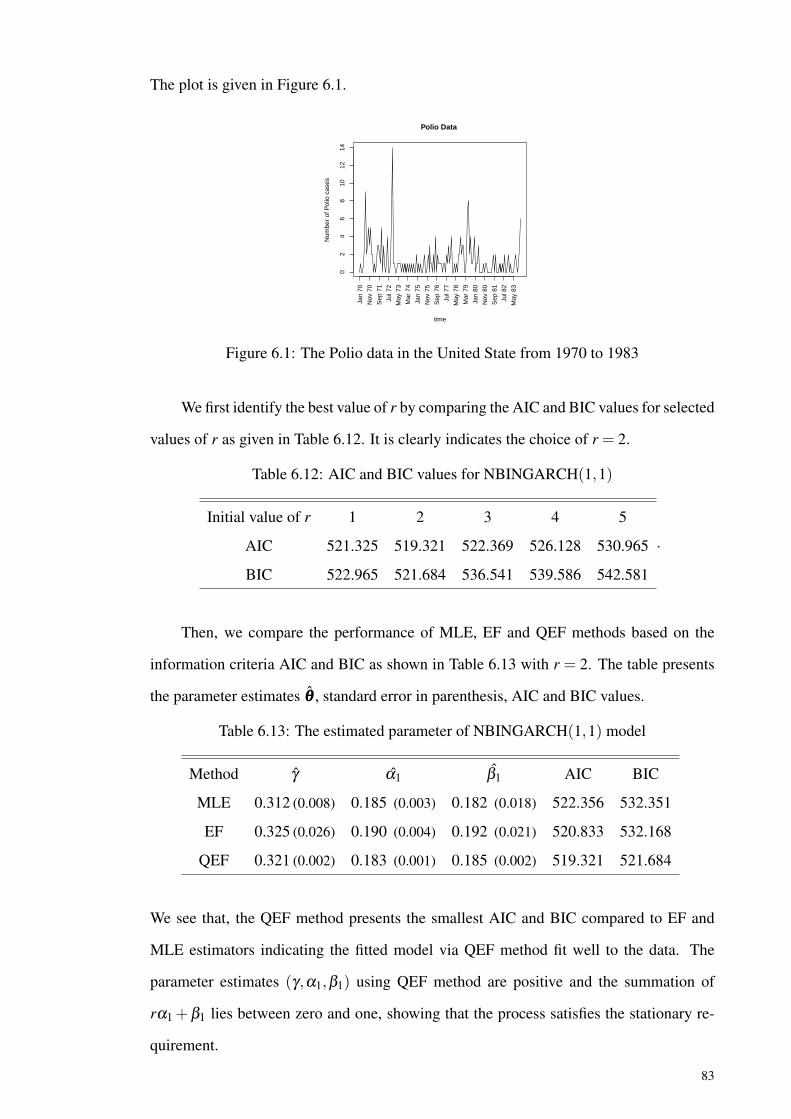
The plot is given in Figure 6.1.
02
46
810
1214
Jan
70
Nov
70
Sep
71
Jul 7
2
May
73
Mar
74
Jan
75
Nov
75
Sep
76
Jul 7
7
May
78
Mar
79
Jan
80
Nov
80
Sep
81
Jul 8
2
May
83
Polio Data
Num
ber
of P
olio
cas
estime
Figure 6.1: The Polio data in the United State from 1970 to 1983
We first identify the best value of r by comparing the AIC and BIC values for selected
values of r as given in Table 6.12. It is clearly indicates the choice of r = 2.
Table 6.12: AIC and BIC values for NBINGARCH(1,1)
Initial value of r 1 2 3 4 5
AIC 521.325 519.321 522.369 526.128 530.965
BIC 522.965 521.684 536.541 539.586 542.581
.
Then, we compare the performance of MLE, EF and QEF methods based on the
information criteria AIC and BIC as shown in Table 6.13 with r = 2. The table presents
the parameter estimates θθθ , standard error in parenthesis, AIC and BIC values.
Table 6.13: The estimated parameter of NBINGARCH(1,1) model
Method γ α1 β1 AIC BIC
MLE 0.312 (0.008) 0.185 (0.003) 0.182 (0.018) 522.356 532.351
EF 0.325 (0.026) 0.190 (0.004) 0.192 (0.021) 520.833 532.168
QEF 0.321 (0.002) 0.183 (0.001) 0.185 (0.002) 519.321 521.684
We see that, the QEF method presents the smallest AIC and BIC compared to EF and
MLE estimators indicating the fitted model via QEF method fit well to the data. The
parameter estimates (γ ,α1,β1) using QEF method are positive and the summation of
rα1 +β1 lies between zero and one, showing that the process satisfies the stationary re-
quirement.
83

From Figure 6.1, it is clearly shown that, the data has an outlier at November 1972,
which indicate that NBINGARCH(1,1) model is preferable compared to INGARCH(1,1)
model. To prove the claim, we then compare the AIC and BIC based on QEF estimates
for INGARCH(1,1) and NBINGARCH(1,1) models.
Table 6.14: AIC and BIC for INGARCH (1,1) and NBINGARCH (1,1) models.
AIC BIC
INGARCH (1,1) 550.23 563.77
NBINGARCH (1,1) 519.321 521.684
The results of AIC and BIC values in Table 6.14 clearly shown that the improvement
of fit with using the NBINGARCH(1,1) model is significant compared to INGARCH(1,1)
model. It indicating such model can deals with both overdispersion and potential extreme
observations. Therefore, we can conclude that NBINGARCH(1,1) model fits the data
better than INGARCH(1,1) model.
In order to check the model adequacy, we first define the residual of the fitted model.
In this NBINGARCH (1,1) process, we define the Pearson residual as
zt =(
Xt − rλt(θθθ))/
√rλt(θθθ)
(1+λt(θθθ)
).
Using such residual zt , we find the mean and variance as 0.0256 and 1.088 respectively
whereby we can clearly see that the mean and variance of this Pearson residuals close to
zero and unity which satisfy the first condition on specified model by Kedem & Fokianos
(2005). To see whether the second condition is satisfied or not, we use the Ljung-Box
(LB) statistics to determine the existence of serial correlation in the data. From Table
6.15, the p-value obtained is greater than the significance level α = 0.05 for both zt
and z2t . Therefore, one can conclude that there is no significant serial correlation in the
residual which satisfies the second requirement. Therefore, the process NBINGARCH
(1,1) is adequate for the data discussed.
84
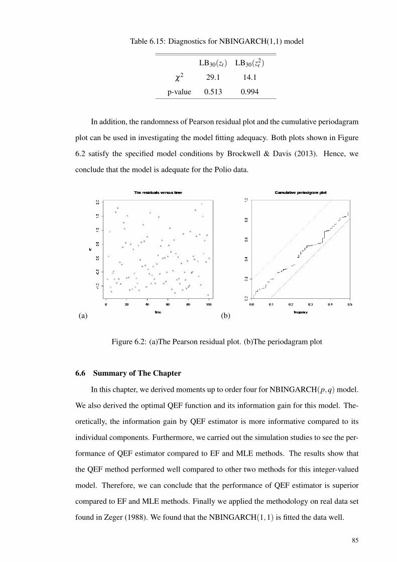
Table 6.15: Diagnostics for NBINGARCH(1,1) model
LB30(zt) LB30(z2t )
χ2 29.1 14.1
p-value 0.513 0.994
In addition, the randomness of Pearson residual plot and the cumulative periodagram
plot can be used in investigating the model fitting adequacy. Both plots shown in Figure
6.2 satisfy the specified model conditions by Brockwell & Davis (2013). Hence, we
conclude that the model is adequate for the Polio data.
(a) (b)
Figure 6.2: (a)The Pearson residual plot. (b)The periodagram plot
6.6 Summary of The Chapter
In this chapter, we derived moments up to order four for NBINGARCH(p,q) model.
We also derived the optimal QEF function and its information gain for this model. The-
oretically, the information gain by QEF estimator is more informative compared to its
individual components. Furthermore, we carried out the simulation studies to see the per-
formance of QEF estimator compared to EF and MLE methods. The results show that
the QEF method performed well compared to other two methods for this integer-valued
model. Therefore, we can conclude that the performance of QEF estimator is superior
compared to EF and MLE methods. Finally we applied the methodology on real data set
found in Zeger (1988). We found that the NBINGARCH(1,1) is fitted the data well.
85

CHAPTER 7
ZIPINGARCH(p,q) MODEL
7.1 Introduction
High occurrence of zeroes in data set may be observed especially in some areas of
public health. For rare diseases with low infection rates, the observed counts typically
contain a high frequency of zeroes (zero-inflation) but the counts can also be very large
during outbreak period. Concerning with this excess zeroes issues, Neyman (1939) and
Feller (1943) introduced the concept of zero-inflation to address the problem of excess
of zeros. Following their findings, many studies and applications of zero-inflated models
have been put forward, especially in regression context. For example, Lambert (1992)
introduced zero-inflated Poisson (ZIP) regression model, Baksh et al. (2011) proposed
the overdispersion test for the ZIP model and Lim et al. (2014) studied the ZIP mixture
regression model.
Extensive studies related to the development of zero-inflated processes are also seen
in time series analysis. A model introduced by Zhu (2012) is known as ZIPINGARCH(p,q)
model. The model is inspired by GARCH (p,q) model with ZIP as conditional distribu-
tion. It is defined as
Xt |ℑXt−1 ∼ ZIP(λt ,ω) , (7.1)
λt = γ +p
∑i=1
αiyt−i +q
∑j=1
β jλt− j (7.2)
where γ > 0, αi ≥ 0, i = 1,2, . . . , p, β j ≥ 0, j = 1,2, . . . ,q, ℑt−1 is the σ -field generated
from Xt−1,Xt−2, . . . ,X1 and the inflation parameter, 0 <ω < 1. Therefore, in this chapter,
we study the ZIP time series model namely ZIPINGARCH(p,q) process focusing on its
moments up to order four and apply the QEF method as the estimation method.
86

7.2 The Moment Properties
Similar as INGARCH(p,q) and NBINGARCH(p,q) models, the moment properties
for conditional and unconditional distributions of ZIPINGARCH(p,q) model are derived.
7.2.1 The Moment Properties of Conditional Distribution in ZIPINGARCH(p,q)Model
In ZIPINGARCH(p,q) model, the conditional distribution follows zero-inflated Pois-
son (ZIP). Let Yt = Xt |ℑXt−1 follows the zero-inflated Poisson distribution with parameter
λt and ω which is Yt ∼ ZIP(λt ,ω) . Zero-inflation models occur when zero counts is
greater than expected for the Poisson distribution. According to Johnson et al. (2005) the
distribution of Poisson known as zero-inflated Poisson where the zero class is misreported
or over reported. The probability mass function (pmf) is
f (yt) =
ω +(1−ω)e−λt for yt = 0
(1−ω)e−λt λ ytt
yt !for yt = 1,2,3, . . .
(7.3)
It is a special case of finite mixture models, that is useful for count data contain-
ing many zeros. The probability generating function is G(z) = ω +(1−ω)eλt(z−1) (see
Johnson et al. (2005) page 353). The mean of such distribution is the first derivatives of
the pgf with z = 1
G′(z) =ddz
[ω +(1−ω)eλt(z−1)
]µt = E(yt) = G′(1) = λt (1−ω)eλt(z−1) = (1−ω)λt .
Using the same step in INGARCH(p,q) and NBINGARCH(p,q), the kth derivative of
ZIP’s pgf is Gk(z) = (1−ω)eλt(z−1)λ kt . To find the variance of ZIP, we first have to obtain
the value of E(y2
t)
whereby from the second derivative of pgf, that is
G′′(1) = E (yt(yt −1)) = E(y2
t)−E(yt) = (1−ω)λ 2
t .
This implies that E(y2
t)= (1−ω)λt (λt +1) and consequently, the variance is given by
σ2yt= E
(y2
t)− [E(yt)]
2 = (1−ω)λt (1+λtω) .
87

By finding the third and fourth derivatives, we can find E(y3
t)
and E(y4
t). We have
G′′′(1) = E (yt(yt −1)(yt −2)) = E(y3
t)−3E
(y2
t)+2E(yt) = (1−ω)λ 3
t and G′′′′(1) =
E (yt(yt −1)(yt −2)(yt −3)) = E(y4
t)−6E
(y3
t)+11E
(y2
t)−6E(yt) = (1−ω)λ 4
t leads
to E(y3
t)= (1−ω)λt
(λ 2
t +3λt +1)
and E(y4
t)= (1−ω)λt
(λ 3
t +6λ 2t +7λt +1
). Us-
ing E(y3
t), we can find the third moment of ZIP model such that
E[(yt − (1−ω)λt)
3]
= E
y3t −3y2
t (1−ω)λt +3yt [(1−ω)λt ]2 − (1−ω)3 λ 3
t
.
Then, using the expectation properties, we have
E[(yt − (1−ω)λt)
3]
= E(y3
t)−3E
(y2
t)(1−ω)λt +3E(yt) [(1−ω)λt ]
2 − (1−ω)3 λ 3t ,
= (1−ω)λt
λ 2t +3λt +1
−3(1−ω)2 λ 2
t λt +1
+3(1−ω)3 λ 3t − (1−ω)3 λ 3
t . (7.4)
Lastly, we factorize Equation (7.4) giving
E[(yt − (1−ω)λt)
3]
= (1−ω)λt
λ 2
t +3λt +1−3(1−ω)λt [λt +1]− (1−ω)2 λ 2t
,
= (1−ω)λt
λ 2
t +3λt +1−3λ 2t −3λt +3ωλ 2
t −3ωλt
+2λ 2t −4λ 2
t ω +2λ 2t ω2
,
= (1−ω)λt
1+3ωλt −λ 2t ω +2λ 2
t ω2 . (7.5)
And, for the fourth moment, apply the same approach, giving
E[(yt − (1−ω)λt)
4]
= E
y4
t −4(1−ω)λty3t +6y2
t (1−ω)2 λ 2t
−4yt (1−ω)3 λ 3t +(1−ω)4 λ 4
t
,
= E(y4
t)−4(1−ω)λtE
(y3
t)+6E
(y2
t)(1−ω)2 λ 2
t
−4E(yt)(1−ω)3 λ 3t +(1−ω)4 λ 4
t . (7.6)
88

Substituting E (yt) , E(y2
t),E(y3
t)
and E(y4
t)
into Equation (7.6), we have
E[(yt − (1−ω)λt)
4]= (1−ω)λt
ωλ 3
t(3ω2 −3ω +1
)+6ω2λ 2
t +λt (4ω +3)+1.
(7.7)
Using (7.5) and the variance, the skewness for ZIP, Γ(ZIP)t can be obtained
Γ(ZIP)t =
E (yt −µt)3
(var(yt))3/2 ,
=(1−ω)λt
1+3ωλt −λ 2
t ω +2λ 2t ω2
[(1−ω)λt (1+λtω)]3/2 ,
=1+3ωλt −λ 2
t ω +2λ 2t ω2√
(1−ω)λt (1+λtω)2. (7.8)
For kurtosis, K(ZIP), we substitute (7.7) and the variance into (D.2) :
K(ZIP) =E (yt −µt)
4
(var(yt))2 ,
=(1−ω)λt
ωλ 3
t(3ω2 −3ω +1
)+6λ 2
t ω2 +λt (4ω +3)+1
[(1−ω)λt (1+λtω)]2,
=ωλ 3
t(3ω2 −3ω +1
)+6λ 2
t ω2 +λt (4ω +3)+1
(1−ω)λt (1+λtω)2 . (7.9)
7.2.2 The Moment Properties of Unconditional Distribution on ZIPINGARCH(p,q)Model
Applying the same approach as in Section (5.2.2) and Section (6.2.2), we first find µ
in terms of λ via mean of the model. The mean of ZIPINGARCH(p,q) is
µ = E(Xt) = E[E(Xt |ℑX
t−1)]
= E [(1−ω)λt ]
and for large t, λt approaches λ , a constant. Hence,
µ = (1−ω)λ . (7.10)
89

Therefore, we rewrite Equation (7.10) as λ = µ1−ω . The variance of the martingale differ-
ence ut is given as
σ2u = E
(u2
t)
= (1−ω)E (λt)+(1−ω)ωE(λ 2
t). (7.11)
On the other hand, the skewness of ut is
Γ(u) =E(u3
t)[
E(u2
t)]3/2 ,
=ω(2ω +1)E
(λ 2
t)+3ωE (λt)+1
E [(1−ω)λt (1+ω (λt))]3/2 (7.12)
Similarly, using the result in Equation (7.12), the excess kurtosis of the process is given
by
K(u) =E(u4
t)[
E(u2
t)]2 −3
=ω(6ω2 −6ω +1)E
(λ 3
t)+6ω(2ω −1)E
(λ 2
t)+7ωE (λt)+1
E ((1−ω)λt)(1+ωλt)2 . (7.13)
Thus, we can rewrite Equations (7.11), (7.12) and (7.13) , therefore, we have the
variance, skewness and kurtosis of ut as
σ2u = µ(1+
ωµ1−ω
), (7.14)
Γ(u) =(1−ω)2 +3µω (1−ω)−µ2ω +2µ2ω2√
(1−ω)µ (1−ω +µω)3, (7.15)
K(u) =ωµ3 (3ω2 −3ω +1
)+6ω2µ2 (1−ω)+µ (1−ω)2 (4ω +3)+(1−ω)3
(1−ω)2 µ (1−ω +µω).
(7.16)
Therefore, the variance, skewness and kurtosis of ZIPINGARCH(p,q) can be obtained
by substituting Equations (7.14), (7.15) and (7.16) into Theorem 1(b), Theorem 2(b) and
90
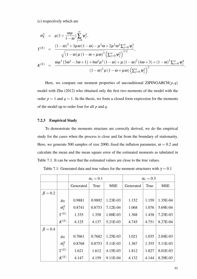
(c) respectively which are
σ2X = µ(1+
ωµ1−ω
)∞
∑j=0
ψ2j ,
Γ(X) =(1−ω)2 +3µω (1−ω)−µ2ω +2µ2ω2 ∑∞
j=0 ψ3j√
(1−ω)µ (1−ω +µω)3(
∑∞j=0 ψ2
j
)3/2 ,
K(X) =ωµ3 (3ω2 −3ω +1
)+6ω2µ2 (1−ω)+µ (1−ω)2 (4ω +3)+(1−ω)3 ∑∞
j=0 ψ4j
(1−ω)2 µ (1−ω +µω)(
∑∞j=0 ψ2
j
)2 .
Here, we compare our moment properties of unconditional ZIPINGARCH(p,q)
model with Zhu (2012) who obtained only the first two moments of the model with the
order p = 1 and q = 1. In the thesis, we form a closed form expression for the moments
of the model up to order four for all p and q.
7.2.3 Empirical Study
To demonstrate the moments structure are correctly derived, we do the empirical
study for the cases when the process is close and far from the boundary of stationarity.
Here, we generate 500 samples of size 2000, fixed the inflation parameter, ω = 0.2 and
calculate the mean and the mean square error of the estimated moments as tabulated in
Table 7.1. It can be seen that the estimated values are close to the true values.
Table 7.1: Generated data and true values for the moment structures with γ = 0.1
α1 = 0.1 α1 = 0.5
Generated True MSE Generated True MSE
β = 0.2
µX 0.9881 0.9892 1.23E-03 1.152 1.159 1.35E-04
σX2 0.8741 0.8753 7.12E-04 1.068 1.076 5.69E-04
Γ(X) 1.335 1.358 1.88E-03 1.368 1.438 7.25E-03
K(X) 4.125 4.137 5.21E-03 4.745 4.751 8.27E-04
β = 0.4
µX 0.7661 0.7682 1.25E-03 1.021 1.035 2.04E-03
σX2 0.8768 0.8753 5.11E-03 1.367 1.355 5.11E-03
Γ(X) 1.621 1.612 4.15E-03 1.812 1.827 8.01E-03
K(X) 4.147 4.159 9.11E-04 4.132 4.144 8.29E-03
91

7.3 Quadratic Estimating Functions on ZIPINGARCH(p,q) Model
In order to apply the QEF method, we first consider the first four conditional mo-
ments of the model (see Liang et al. (2011)). The mean, variance, skewness and kurtosis
of yt conditional on ℑXt−1 of ZIPINGARCH(p,q) model are
µt(θθθ) = (1−ω)λt(θθθ),
σ2t (θθθ) = (1−ω)λt(θθθ)(1+ωλt(θθθ)) ,
Γ(θθθ) =ω(2ω +1)λ 2
t (θθθ)+3ωλt(θθθ)+1
((1−ω)λt(θθθ))1/2 (1+ωλt(θθθ))3/2 ,
κ(θθθ) =ω(6ω2 −6ω +1)λ 3
t (θθθ)+6ω(2ω −1)λ 2t (θθθ)+7ωλt(θθθ)+1
((1−ω)λt(θθθ))(1+ωλt(θθθ))2 .
Then, by taking the martingale differences as mt(θθθ) = yt −µt(θθθ), st(θθθ) = m2t (θθθ)−
σ2t (θθθ), we have ⟨m⟩t = σ2
t (θθθ), ⟨s⟩t = σ4t (θθθ)(κt(θθθ)+2) and ⟨m,s⟩t = σ3
t (θθθ)γt(θθθ). Using
arguments similar to those in the other models, the derivatives of mean and variance with
respect to θθθ , ∂ µt(θθθ)∂θ and ∂σ2
t (θθθ)∂θ are
∂ µt(θθθ)∂θθθ
=
(−λt ,(1−ω)
∂λt
∂α0, . . . ,(1−ω)
∂λt
∂αp,(1−ω)
∂λt
∂β1, . . . ,(1−ω)
∂λt
∂βq
)′
,
=(A1,t ,A2,t ,A(3,1,t), . . . ,A(3,p,t), . . . ,A(4,1,t), . . . ,A(4,q,t)
)′.
∂σ2t (θθθ)
∂θθθ=
(−λt(1+2ωλt),Rt
∂λt∂α0
, . . . ,Rt∂λt∂αp
,Rt∂λt∂β1
, . . . ,Rt∂λt∂βq
,
)′
,
=(S1,t ,S2,t ,S(3,1,t), . . . ,S(3,p,t), . . . ,S(4,1,t), . . . ,S(4,q,t),
)′.
where define Rt = (1 − ω)(1 + 2ωλt(θθθ)), A(i, j,t) is the partial derivative of the mean
with respect to each parameter and S(i, j,t) is the partial derivative of the variance with
respect to each parameter. Now, we let Amk,t =
−Ak⟨m⟩t , Sm
k,t =Sk⟨m,s⟩t⟨m⟩t⟨s⟩t
, Pvk,t =
Ak⟨m,s⟩t⟨m⟩t⟨s⟩t , and
Qvk,t =
−Sk⟨s⟩t .Hence, the optimal estimating function is given by
g∗Q(θθθ) =n
∑t=1
(a∗t−1mt +b∗t−1st),
92
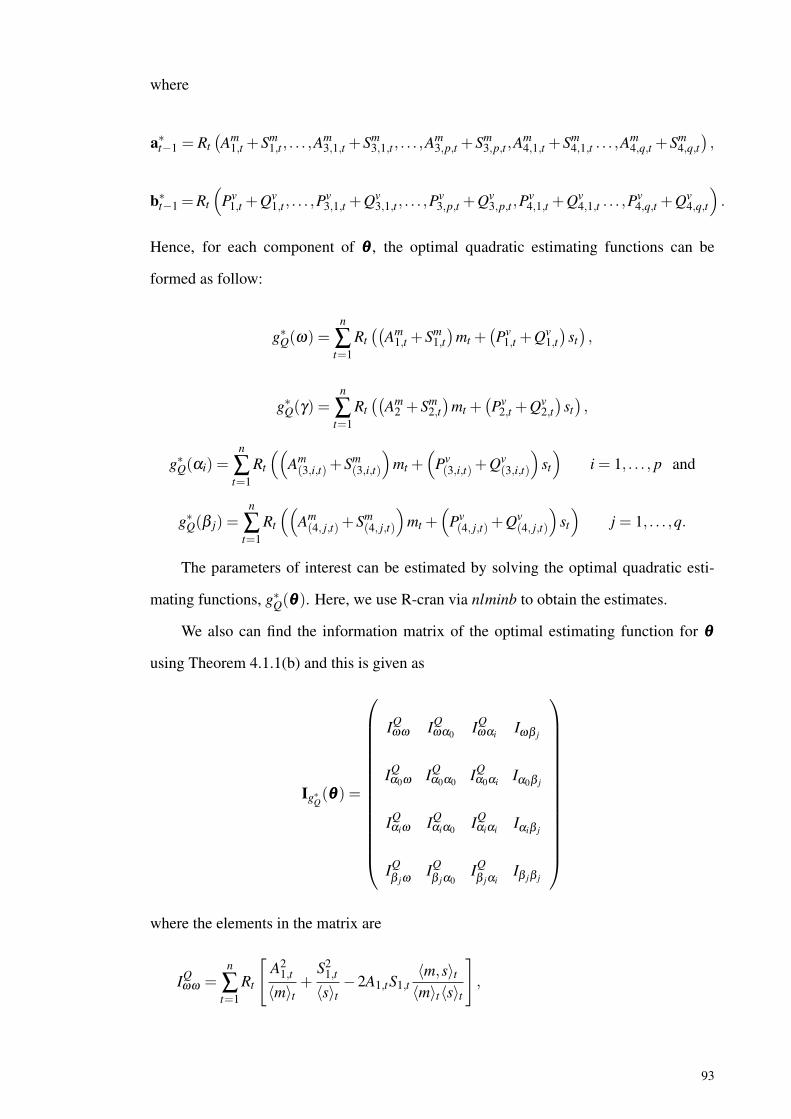
where
a∗t−1 = Rt(Am
1,t +Sm1,t , . . . ,A
m3,1,t +Sm
3,1,t , . . . ,Am3,p,t +Sm
3,p,t ,Am4,1,t +Sm
4,1,t . . . ,Am4,q,t +Sm
4,q,t),
b∗t−1 =Rt
(Pv
1,t +Qv1,t , . . . ,P
v3,1,t +Qv
3,1,t , . . . ,Pv3,p,t +Qv
3,p,t ,Pv4,1,t +Qv
4,1,t . . . ,Pv4,q,t +Qv
4,q,t
).
Hence, for each component of θθθ , the optimal quadratic estimating functions can be
formed as follow:
g∗Q(ω) =n
∑t=1
Rt((
Am1,t +Sm
1,t)
mt +(Pv
1,t +Qv1,t)
st),
g∗Q(γ) =n
∑t=1
Rt((
Am2 +Sm
2,t)
mt +(Pv
2,t +Qv2,t)
st),
g∗Q(αi) =n
∑t=1
Rt
((Am(3,i,t)+Sm
(3,i,t)
)mt +
(Pv(3,i,t)+Qv
(3,i,t)
)st
)i = 1, . . . , p and
g∗Q(β j) =n
∑t=1
Rt
((Am(4, j,t)+Sm
(4, j,t)
)mt +
(Pv(4, j,t)+Qv
(4, j,t)
)st
)j = 1, . . . ,q.
The parameters of interest can be estimated by solving the optimal quadratic esti-
mating functions, g∗Q(θθθ). Here, we use R-cran via nlminb to obtain the estimates.
We also can find the information matrix of the optimal estimating function for θθθ
using Theorem 4.1.1(b) and this is given as
Ig∗Q(θθθ) =
IQωω IQ
ωα0 IQωαi Iωβ j
IQα0ω IQ
α0α0 IQα0αi Iα0β j
IQαiω IQ
αiα0 IQαiαi Iαiβ j
IQβ jω IQ
β jα0IQβ jαi
Iβ jβ j
where the elements in the matrix are
IQωω =
n
∑t=1
Rt
[A2
1,t
⟨m⟩t+
S21,t
⟨s⟩t−2A1,tS1,t
⟨m,s⟩t
⟨m⟩t⟨s⟩t
],
93

IQα0α0 =
n
∑t=1
Rt
[A2
1,t
⟨m⟩t+
S22,t
⟨s⟩t−2A2,tS2,t
⟨m,s⟩t
⟨m⟩t⟨s⟩t
],
IQαiαi =
n
∑t=1
Rt
[A2(3,i,t)
⟨m⟩t+
S2(3,i,t)
⟨s⟩t−2A(3,i,t)S(3,i,t)
⟨m,s⟩t
⟨m⟩t⟨s⟩t
],
IQβ jβ j
=n
∑t=1
Rt
[A2(4, j,t)
⟨m⟩t+
S2(4, j,t)
⟨s⟩t−2A(4, j,t)S(4, j,t)
⟨m,s⟩t
⟨m⟩t⟨s⟩t
],
IQωα0 =
n
∑t=1
Rt
[A1,tA2,t
⟨m⟩t+
S1,tS2,t
⟨s⟩t− (A1,tS2,t +S1,tA2,t)
⟨m,s⟩t
⟨m⟩t⟨s⟩t
]IQωαi =
n
∑t=1
Rt
[A1,tA(3,i,t)
⟨m⟩t+
S1,tS(3,i,t)⟨s⟩t
− (A1,tS(3,i,t)+S1,tA(3,i,t))⟨m,s⟩t
⟨m⟩t⟨s⟩t
],
IQωβ j
=n
∑t
Rt
[A1,tA(4,i)
⟨m⟩t+
S1,tS(4,i)⟨s⟩t
− (A1,tS(4,i,t)+S1,tA(4,i,t))⟨m,s⟩t
⟨m⟩t⟨s⟩t
],
IQα0αi =
n
∑t=1
Rt
[A(3,i,t)A2,t
⟨m⟩t+
S(3,i,t)S2,t
⟨s⟩t− (A2,tS(3,i,t)+S2,tA(3,i,t))
⟨m,s⟩t
⟨m⟩t⟨s⟩t
],
IQα0β j
=n
∑t=1
Rt
[A(4, j,t)A2,t
⟨m⟩t+
S(4, j,t)S2,t
⟨s⟩t− (A2,tS(4, j,t)+S2,tA(4, j,t))
⟨m,s⟩t
⟨m⟩t⟨s⟩t
],
IQαiβ j
=n
∑t=1
Rt
[A(3,i,t)A(4, j,t)
⟨m⟩t+
A(3, j)S(4, j,t)⟨s⟩t
− (A(3,i,t)S(4, j,t)+S(3,i,t)A(4, j,t))⟨m,s⟩t
⟨m⟩t⟨s⟩t
]
and remaining elements can be obtained by the symmetry of the matrix: Iα0ω = Iωα0 ,
Iαiω = Iωαi , Iβ jω = Iωβ j , Iαiα0 = Iα0αi , Iβ jα0 = Iα0β j and Iβ jαi = Iαiβ j .
In addition, we can also derive the optimal estimating function mt which is given by
g∗m(θ) =−n
∑t=1
∂ µt (θθθ)∂θθθ
Xt − (1−ω)λt (θθθ)
(1−ω)λt (θθθ)(1+(1−ω)λt (θθθ))
(7.17)
and the optimal estimating function on st given by
g∗s (θ) =−n
∑t=1
∂σ2t (θθθ)∂θθθ
m2
t (θθθ)−σ4t (θθθ)
σ4t (κt +2)
. (7.18)
Then, the corresponding information matrices for mt(θθθ) and st(θθθ) identified as Ig∗m(θθθ)
and Ig∗s (θθθ) respectively are
94
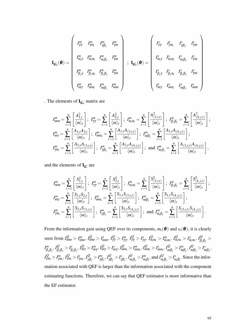
Ig∗m(θθθ) =
Imγγ Im
γαiImγβ j
Imγω
Imαiγ Im
αiαiImαiβ j
Imγω
Imβ jγ Im
β jαiImβ jβ j
Imγω
Imωγ Im
ωαiImωβ j
Imωω
; Ig∗m(θθθ) =
Isγγ Is
γαiIsγβ j
Isγω
Isαiγ Is
αiαiIsαiβ j
Isγω
Isβ jγ Is
β jαiIsβ jβ j
Isγω
Isωγ Is
ωαiIsωβ j
Isωω
. The elements of Ig∗m matrix are
Imωω =
n
∑t=1
[A2
1,t
⟨m⟩t
]; Im
γγ =n
∑t=1
[A2
2,t
⟨m⟩t
]; Im
αiαi=
n
∑t=1
[A2(3,i,t)
⟨m⟩t
]; Im
β jβ j=
n
∑t=1
[A2(4, j,t)
⟨m⟩t
];
Imωγ =
n
∑t=1
[A1,tA2,t
⟨m⟩t
]; Im
ωαi=
n
∑t=1
[A1,tA(3,i,t)
⟨m⟩t
]; Im
ωβ j=
n
∑t=1
[A1,tA(4, j,t)
⟨m⟩t
];
Imγαi
=n
∑t=1
[A2,tA(3,i,t)
⟨m⟩t
]; Im
γβ j=
n
∑t=1
[A2,tA(4, j,t)
⟨m⟩t
]; and Im
αiβ j=
n
∑t=1
[A(3,i,t)A(4, j,t)
⟨m⟩t
],
and the elements of Ig∗s are
Imωω =
n
∑t=1
[S2
1,t
⟨m⟩t
]; Im
γγ =n
∑t=1
[S2
2,t
⟨m⟩t
]; Im
αiαi=
n
∑t=1
[S2(3,i,t)
⟨m⟩t
]; Im
β jβ j=
n
∑t=1
[S2(4, j,t)
⟨m⟩t
];
Imωγ =
n
∑t=1
[S1,tS2,t
⟨m⟩t
]; Im
ωαi=
n
∑t=1
[S1,tS(3,i,t)⟨m⟩t
]; Im
ωβ j=
n
∑t=1
[S1,tS(4, j,t)
⟨m⟩t
];
Imγαi
=n
∑t=1
[S2,tS(3,i,t)⟨m⟩t
]; Im
γβ j=
n
∑t=1
[S2,tS(4, j,t)
⟨m⟩t
]; and Im
αiβ j=
n
∑t=1
[S(3,i,t)S(4, j,t)
⟨m⟩t
].
From the information gain using QEF over its components, mt(θθθ) and st(θθθ), it is clearly
seen from IQωω > Im
ωω , IQωω > Is
ωω , IQγγ > Im
γγ , IQγγ > Is
γγ , IQαiαi > Im
αiαi, IQ
αiαi > Isαiαi
, IQβ jβ j
>
Imβ jβ j
, IQβ jβ j
> Isβ jβ j
, IQωγ > Im
ωγ , IQωγ > Is
ωγ , IQωαi > Im
ωαi, IQ
ωαi > Isωαi
, IQωβ j
> Imωβ j
, IQωβ j
> Isωβ j
,
IQγαi > Im
γαi, IQ
γαi > Isγαi
, IQγβ j
> Imγβ j
, IQγβ j
> Isγβ j
, IQαiβ j
> Imαiβi
, and IQαiβ j
> Isαiβi
. Since the infor-
mation associated with QEF is larger than the information associated with the component
estimating functions. Therefore, we can say that QEF estimator is more informative than
the EF estimator.
95
7.4 Performance of The Estimation Methods on ZIPINGARCH (1,1)
To evaluate the performance of QEF, MLE and EF methods, a simulation study on
ZIPINGARCH (1,1) was carried out with the inflation parameter ω = 0.2, replication
N = 500, and two sample sizes, n = 100 and n = 2000. The process is defined as
Xt |ℑXt−1 ∼ ZIP(λt ,ω) , (7.19)
λt = γ +α1Xt−1 +β1λt−1. (7.20)
7.4.1 MLE Derivation of ZIPINGARCH (1,1)
Since ZIPINGARCH (1,1) has two separate probability mass functions (pmf), the
loglikelihood for a model has two parts namely
L =
∑∞
t=1 ln
ω +(1−ω)e−λt
for Xt = 0,
∑∞t=1 ln (1−ω)−λt +Xt ln λt − ln(Xt!) for Xt = 1,2,3, . . .
(7.21)
We then maximized the loglikelihood to extract the estimated parameter of interest in
R-cran.
7.4.2 EF Derivation of ZIPINGARCH (1,1)
Using the same approach as Section 6.4.2, we derive the optimal EF function through
Equation (7.17). The derivative of mean, µt with respect to θθθ given in following form
∂ µt (θθθ)∂θθθ
=
λt for θ = ω
−(1−ω)λ ′t for θ = γ,α1,β1.
(7.22)
Hence, from Theorem 1, the optimal for each component g∗E(θθθ) of the model are:
g∗E(γ) =n
∑t=1
[−1−β1
dλtdγγγ
λt (1+ωλt)
(Xt − (1−ω)λt)
], (7.23)
g∗E(αi) =n
∑t=1
[−Xt−1 −β1
dλtdααα1
λt (1+ωλt)
(Xt − (1−ω)λt)
], (7.24)
g∗E(β j) =n
∑t=1
−λt−1 −β1dλtdβββ 1
λt (1+ωλt)
(Xt − (1−ω)λt)
, (7.25)
96
g∗E(ω) =n
∑t=1
[Xt − (1−ω)λt
(1−ω)(1+λtω)
]. (7.26)
We solve the simultaneous Equation of optimal g∗E = 0 using nleqslv command in R-cran
to get the estimates of interest.
7.4.3 QEF Derivation of ZIPINGARCH (1,1)
For the QEF method on the model, we use the derivation in Section (7.3) which leads
to
g∗Q(ω) =n
∑t=1
Rt((
Am1,t +Sm
1,t)
mt +(Pv
1,t +Qv1,t)
st),
g∗Q(γ) =n
∑t=1
Rt((
Am2,t +Sm
2,t)
mt +(Pv
2,t +Qv2,t)
st),
g∗Q(α1) =n
∑t=1
Rt
((Am(3,1,t)+Sm
(3,1,t)
)mt +
(Pv(3,1,t)+Qv
(3,1,t)
)st
)and
g∗Q(β1) =n
∑t=1
Rt
((Am(4,1,t)+Sm
(4,1,t)
)mt +
(Pv(4,1,t)+Qv
(4,1,t)
)st
).
Again, we solve such simultaneous Equation g∗E = 0 using nlesqv command in R-cran
software.
7.4.4 Simulation Study
The steps of QEF algorithm for ZIPINGARCH (1,1) are almost the same as in Sec-
tion 5.4.3. Since we have one extra parameter, ω , in this model, in Step 1, the data are
generated for a given value of the vectors of parameters (ω ,γ,α1,β1). In Step 2, the IN-
GARCH (1,1) model will be changed to ZIPINGARCH (1,1) model and for Step 3, we
use the similar method as in Section 6.4.4.
7.4.5 The Result
The performance is measured based on the mean, bias, standard error(SE) and mean
squared error (MSE) from the repetitions (N = 500) for each parameter from EF, MLE
and QEF estimators. These are shown in Tables 7.2-7.11 .
97

Discussion
Since the MLE for this model does not have a closed form, we need to search for
the maximum value of the likelihood function. Note that in this model the likelihood is
divided into two parts with the zero and nonzero observed data. Therefore, the EF and
QEF methods are computationally more efficient and easy to apply in practice than MLE
method.
From Tables 7.2-7.11, we can see that, in term of biasness, the QEF method pro-
duce the smallest bias compared to other two methods. Furthermore, the QEF method
produce the better result in terms of estimated bias, standard error and mean square error
compared to EF estimator in all tables, either small sample size, n = 100 or large sam-
ple sizes, n = 1500 and n = 2000. The simulation results obtained support theoretical
results observed earlier in the study. Therefore, we can conclude that the QEF estimator
is superior compared to EF estimator.
On the other hand, although MLE method gives slightly smaller value of standard
errors mean square errors compared EF and QEF methods in some cases, specifically we
can see from Table 7.2-7.6, which are satisfied the stationarity condition, but the values
increase as the combination set of parameters approach the non-stationarity conditions
as shown in Table 7.7-7.11. Compared with EF and QEF methods, the value remain
small and do have no effect on these combination set of parameters for all sample sizes.
Therefore, we can say that, the EF and QEF estimators are better compared to MLE
method for ZIPINGARCH(1,1) case.
Therefore, from the results obtained, we can say that the QEF method performs well
compared to EF and MLE methods. Hence, we can conclude that, the QEF estimator is
better estimation method in this IVTS model.
98

Tabl
e7.
2:Si
mul
atio
nre
sults
forZ
IPIN
GA
RC
H(1,1)
with
γ=
0.1,
α 1=
0.2,
and
β 1=
0.3
n=10
0n=
1500
n=20
00
ML
EF
QE
FM
LE
FQ
EF
ML
EF
QE
F
γ
Mea
n0.
049
0.05
10.
055
0.07
0.10
90.
108
0.06
90.
106
0.10
4
Bia
s0.
051
0.04
90.
045
0.03
00.
009
0.00
80.
031
0.00
60.
004
SE0.
087
0.09
10.
082
0.03
00.
056
0.03
20.
015
0.01
60.
015
MSE
5.23
E-0
35.
85E
-03
5.38
E-0
31.
30E
-03
1.72
E-0
31.
49E
-03
1.17
E-0
31.
19E
-03
1.08
e-03
α 1
Mea
n0.
108
0.10
70.
122
0.13
90.
210
0.19
70.
138
0.19
30.
199
Bia
s0.
092
0.09
30.
078
0.06
10.
010
0.00
30.
062
0.00
70.
001
SE0.
075
0.07
90.
069
0.04
70.
064
0.05
40.
041
0.04
20.
033
MSE
8.54
E-0
38.
66E
-03
8.50
E-0
32.
53E
-03
2.82
E-0
31.
39E
-03
1.02
E-0
31.
09E
-03
1.02
e-03
β 1
Mea
n0.
353
0.35
50.
350
0.32
10.
326
0.29
70.
322
0.31
10.
302
Bia
s0.
053
0.05
50.
050
0.02
10.
026
0.00
30.
022
0.01
10.
002
SE0.
152
0.15
0.14
40.
076
0.08
20.
074
0.07
50.
075
0.05
8
MSE
6.31
E-0
36.
37E
-03
6.28
E-0
32.
22E
-03
2.84
E-0
31.
87E
-03
1.19
E-0
31.
18E
-03
1.05
e-03
ω
Mea
n0.
221
0.22
80.
218
0.18
80.
233
0.20
80.
188
0.22
80.
203
Bia
s0.
021
0.02
80.
018
0.01
20.
033
0.00
80.
012
0.02
80.
003
SE0.
099
0.11
40.
095
0.02
40.
096
0.04
20.
016
0.02
90.
013
MSE
5.37
E-0
36.
21E
-03
5.44
E-0
31.
74E
-03
2.42
E-0
31.
14E
-03
1.04
E-0
31.
09E
-03
1.02
e-03
99

Tabl
e7.
3:Si
mul
atio
nre
sults
forZ
IPIN
GA
RC
H(1,1)
with
γ=
0.2,
α 1=
0.4,
and
β 1=
0.1
n=10
0n=
1500
n=20
00
ML
EF
QE
FM
LE
FQ
EF
ML
EF
QE
F
γ
Mea
n0.
139
0.14
20.
148
0.15
70.
182
0.19
30.
158
0.19
60.
198
Bia
s0.
061
0.05
80.
052
0.04
30.
018
0.00
70.
042
0.00
40.
002
SE0.
078
0.08
10.
079
0.04
30.
087
0.03
60.
038
0.03
80.
015
MSE
9.31
E-0
39.
52E
-03
9.38
E-0
33.
62E
-03
4.34
E-0
32.
42E
-03
2.48
E-0
32.
42E
-03
1.87
e-03
α 1
Mea
n0.
316
0.32
40.
416
0.31
60.
324
0.41
60.
317
0.39
63.
999e
-01
Bia
s0.
084
0.07
60.
016
0.08
40.
076
0.01
60.
083
0.00
41.
02e-
04
SE0.
065
0.07
50.
055
0.06
50.
075
0.05
50.
060
0.06
10.
013
MSE
1.14
E-0
31.
17E
-03
1.15
E-0
31.
14E
-03
1.17
E-0
31.
15E
-03
1.07
E-0
31.
07E
-03
1.02
e-03
β 1
Mea
n0.
153
0.15
50.
151
0.11
90.
115
0.11
10.
119
0.10
70.
104
Bia
s0.
053
0.05
50.
051
0.01
90.
015
0.01
10.
019
0.00
70.
004
SE0.
096
0.09
20.
083
0.01
50.
021
0.01
30.
013
0.01
40.
004
MSE
1.23
E-0
22.
11E
-02
9.88
E-0
37.
05E
-03
7.47
E-0
33.
82E
-03
2.01
E-0
32.
02E
-03
1.39
e-03
ω
Mea
n0.
092
0.09
90.
106
0.10
90.
180
0.18
80.
107
0.18
50.
194
Bia
s0.
108
0.10
10.
094
0.09
10.
020
0.01
20.
093
0.01
50.
006
SE0.
095
0.09
10.
085
0.07
00.
080
0.00
70.
042
0.03
90.
002
MSE
7.28
E-0
37.
31E
-03
7.26
E-0
31.
64E
-03
4.23
E-0
31.
66E
-03
1.05
E-0
31.
24E
-03
1.07
e-03
100

Tabl
e7.
4:Si
mul
atio
nre
sults
forZ
IPIN
GA
RC
H(1,1)
with
γ=
0.3,
α 1=
0.1,
and
β 1=
0.4
n=10
0n=
1500
n=20
00
ML
EF
QE
FM
LE
FQ
EF
ML
EF
QE
F
γ
Mea
n0.
217
0.22
00.
228
0.24
10.
305
0.30
20.
235
0.30
20.
301
Bia
s0.
083
0.08
00.
072
0.05
90.
005
0.00
20.
065
0.00
27.
22e-
04
SE0.
082
0.07
50.
066
0.03
70.
010
0.00
50.
008
0.00
70.
001
MSE
9.27
E-0
39.
31E
-03
9.11
E-0
33.
93E
-03
5.24
E-0
32.
39E
-03
1.15
E-0
31.
16E
-03
1.03
e-03
α 1
Mea
n0.
045
0.04
70.
052
0.07
00.
088
0.10
70.
071
0.09
10.
101
Bia
s0.
055
0.05
30.
038
0.03
00.
012
0.00
70.
029
0.00
90.
001
SE0.
087
0.08
20.
075
0.02
90.
039
0.02
20.
015
0.01
90.
017
MSE
5.11
E-0
35.
31E
-03
5.18
E-0
31.
75E
-03
2.75
E-0
31.
15E
-03
1.02
E-0
31.
02E
-03
9.05
e-04
β 1
Mea
n0.
325
0.35
90.
341
0.42
70.
419
0.41
70.
437
0.40
80.
402
Bia
s0.
075
0.07
10.
059
0.02
70.
019
0.01
70.
037
0.00
80.
002
SE0.
075
0.07
10.
064
0.02
50.
063
0.05
00.
013
0.01
50.
009
MSE
6.31
E-0
36.
88E
-03
6.32
E-0
33.
21E
-03
3.87
E-0
33.
53E
-03
1.13
E-0
31.
16E
-03
1.08
e-03
ω
Mea
n0.
147
0.15
10.
159
0.18
00.
233
0.22
70.
179
0.21
40.
201
Bia
s0.
053
0.04
90.
041
0.02
00.
033
0.02
70.
021
0.01
40.
001
SE0.
076
0.07
30.
071
0.05
10.
040
0.02
90.
044
0.03
10.
015
MSE
7.39
E-0
37.
54E
-03
7.41
E-0
33.
17E
-03
3.77
E-0
31.
46E
-03
1.21
E-0
31.
27E
-03
1.01
e-03
101

Tabl
e7.
5:Si
mul
atio
nre
sults
forZ
IPIN
GA
RC
H(1,1)
with
γ=
0.3,
α 1=
0.4,
and
β 1=
0.2
n=10
0n=
1500
n=20
00
ML
EF
QE
FM
LE
FQ
EF
ML
EF
QE
F
γ
Mea
n0.
181
0.18
20.
191
0.21
10.
272
0.27
90.
211
0.28
70.
294
Bia
s0.
119
0.11
80.
109
0.08
90.
028
0.02
10.
089
0.01
30.
006
SE0.
062
0.05
90.
055
0.04
50.
050
0.03
70.
012
0.02
40.
011
MSE
7.32
E-0
37.
85E
-03
7.46
E-0
31.
61E
-03
1.52
E-0
31.
47E
-03
1.27
E-0
31.
25E
-03
1.01
e-03
α 1
Mea
n0.
308
0.31
20.
324
0.33
50.
363
0.37
80.
351
0.38
50.
408
Bia
s0.
092
0.08
80.
076
0.06
50.
037
0.02
20.
049
0.01
50.
008
SE0.
089
0.08
50.
076
0.04
10.
051
0.04
50.
037
0.04
10.
032
MSE
8.13
E-0
38.
28E
-03
8.09
E-0
32.
68E
-03
2.75
E-0
32.
65E
-03
1.09
E-0
31.
10E
-03
1.04
e-03
β 1
Mea
n0.
252
0.24
80.
239
0.22
30.
221
0.21
00.
223
0.21
10.
205
Bia
s0.
052
0.04
80.
039
0.02
30.
021
0.01
00.
023
0.01
10.
005
SE0.
121
0.12
80.
118
0.09
10.
097
0.01
20.
046
0.05
00.
007
MSE
8.36
E-0
38.
43E
-03
8.15
E-0
35.
01E
-03
6.20
E-0
33.
93E
-03
1.11
E-0
31.
10E
-36
1.02
e-03
ω
Mea
n0.
253
0.25
60.
252
0.19
70.
196
0.20
20.
199
0.20
10.
201
Bia
s0.
053
0.05
40.
052
0.00
30.
004
0.00
20.
001
0.00
17.
23E
-04
SE0.
082
0.07
90.
062
0.04
20.
074
0.02
20.
037
0.03
80.
012
MSE
8.15
E-0
38.
21E
-03
7.03
E-0
32.
14E
-03
3.21
E-0
31.
82E
-03
1.07
E-0
31.
08E
-03
7.52
e-04
102

Tabl
e7.
6:Si
mul
atio
nre
sults
forZ
IPIN
GA
RC
H(1,1)
with
γ=
0.5,
α 1=
0.2,
and
β 1=
0.3
n=10
0n=
1500
n=20
00
ML
EF
QE
FM
LE
FQ
EF
ML
EF
QE
F
γ
Mea
n0.
432
0.43
70.
442
0.45
50.
452
0.47
40.
443
0.48
60.
490
Bia
s0.
068
0.06
30.
058
0.04
50.
048
0.02
60.
056
0.01
40.
010
SE0.
043
0.03
90.
031
0.01
40.
031
0.02
60.
011
0.01
30.
012
MSE
7.35
E-0
37.
52E
-03
7.39
E-0
34.
22E
-03
4.52
E-0
34.
24E
-03
1.92
E-0
31.
92E
-03
1.12
e-03
α 1
Mea
n0.
129
0.13
20.
143
0.13
80.
175
0.18
20.
137
0.18
50.
197
Bia
s0.
071
0.06
80.
057
0.06
20.
025
0.01
80.
063
0.01
50.
003
SE0.
066
0.06
20.
049
0.03
10.
056
0.03
80.
027
0.04
70.
026
MSE
5.19
E-0
35.
27E
-03
5.03
E-0
31.
04E
-03
1.23
E-0
31.
09E
-03
7.94
E-0
48.
27E
-04
7.99
e-04
β 1
Mea
n0.
391
0.38
80.
371
0.35
10.
364
0.36
10.
362
0.31
70.
309
Bia
s0.
091
0.08
80.
071
0.05
20.
064
0.06
10.
062
0.01
70.
009
SE0.
062
0.05
60.
044
0.01
70.
032
0.01
30.
013
0.02
0.01
0
MSE
7.12
E-0
36.
53E
-03
6.19
E-0
32.
47E
-03
2.40
E-0
31.
64E
-03
9.57
E-0
49.
54E
-04
8.11
e-04
ω
Mea
n0.
159
0.15
90.
165
0.19
00.
230
0.21
00.
190
0.22
10.
215
Bia
s0.
041
0.04
10.
035
0.01
00.
030
0.01
00.
010
0.02
10.
005
SE0.
076
0.07
30.
059
0.03
00.
039
0.01
80.
018
0.01
40.
008
MSE
9.01
E-0
39.
25E
-03
9.08
E-0
31.
09E
-03
1.18
E-0
31.
02E
-03
8.07
E-0
48.
08E
-04
7.39
e-04
103

Tabl
e7.
7:Si
mul
atio
nre
sults
forZ
IPIN
GA
RC
H(1,1)
with
γ=
0.1,
α 1=
0.6,
and
β 1=
0.3
n=10
0n=
1500
n=20
00
ML
EF
QE
FM
LE
FQ
EF
ML
EF
QE
F
γ
Mea
n0.
017
0.04
10.
048
0.06
90.
115
0.08
90.
069
0.10
80.
101
Bia
s0.
083
0.05
90.
052
0.03
10.
015
0.01
10.
031
0.00
80.
001
SE0.
689
0.12
70.
119
0.41
10.
029
0.02
40.
309
0.01
0.00
8
MSE
3.68
E-0
18.
32E
-03
7.11
E-0
31.
95E
-02
2.58
E-0
32.
02E
-03
1.16
E-0
21.
18E
-03
1.03
e-03
α 1
Mea
n0.
542
0.56
80.
576
0.58
20.
612
0.59
00.
582
0.59
20.
597
Bia
s0.
058
0.03
20.
024
0.01
80.
012
0.01
00.
018
0.00
80.
003
SE0.
612
0.09
10.
082
0.44
30.
081
0.05
00.
438
0.03
90.
014
MSE
9.88
E-0
28.
23E
-03
8.01
E-0
36.
84E
-02
7.96
E-0
35.
78E
-03
1.77
E-0
21.
81E
-03
1.11
e-03
β 1
Mea
n0.
241
0.27
90.
282
0.32
10.
290
0.29
40.
321
0.29
30.
299
Bia
s0.
059
0.02
10.
018
0.02
10.
010
0.00
60.
021
0.00
70.
001
SE0.
581
0.10
20.
085
0.44
10.
048
0.04
00.
435
0.03
50.
016
MSE
1.23
E-0
21.
33E
-03
1.08
E-0
37.
21E
-02
7.20
E-0
35.
60E
-03
2.23
E-0
22.
25E
-03
1.26
e-03
ω
Mea
n0.
148
0.17
90.
181
0.18
00.
188
0.18
90.
230
0.20
80.
203
Bia
s0.
052
0.02
10.
019
0.02
00.
012
0.01
10.
030
0.00
80.
003
SE0.
613
0.11
30.
089
0.41
40.
019
0.01
30.
411
0.01
00.
005
MSE
9.78
E-0
28.
52E
-03
6.32
E-0
31.
46E
-02
2.50
E-0
31.
51E
-03
1.01
E-0
21.
02E
-03
9.68
e-04
104

Tabl
e7.
8:Si
mul
atio
nre
sults
forZ
IPIN
GA
RC
H(1,1)
with
γ=
0.1,
α 1=
0.7,
and
β 1=
0.2
n=10
0n=
1500
n=20
00
ML
EF
QE
FM
LE
FQ
EF
ML
EF
QE
F
γ
Mea
n0.
018
0.15
20.
069
0.07
20.
105
9.95
E-0
20.
072
0.10
40.
1001
Bia
s0.
082
0.05
20.
031
0.02
80.
005
0.00
050.
028
0.00
40.
0001
SE0.
813
0.07
20.
065
0.41
20.
027
0.01
70.
410
0.01
50.
010
MSE
8.88
E-0
29.
35E
-03
7.21
E-0
31.
59E
-02
2.79
E-0
32.
38E
-03
1.02
E-0
21.
19E
-03
1.02
e-03
α 1
Mea
n0.
646
0.72
10.
713
0.68
90.
719
0.68
90.
680.
689
0.69
4
Bia
s0.
054
0.02
10.
013
0.01
10.
019
0.01
10.
020.
011
0.00
6
SE0.
612
0.21
30.
201
0.45
40.
089
0.02
80.
426
0.02
90.
019
MSE
2.31
E-0
12.
51E
-02
1.08
E-0
27.
59E
-02
6.93
E-0
32.
48E
-03
2.66
E-0
22.
63E
-03
1.26
e-03
β 1
Mea
n0.
251
0.23
20.
225
0.22
20.
220
0.21
10.
222
0.20
90.
195
Bia
s0.
051
0.03
20.
025
0.02
20.
020
0.01
10.
022
0.00
90.
005
SE0.
852
0.14
70.
099
0.44
90.
055
0.04
10.
422
0.03
20.
007
MSE
7.53
E-0
29.
18E
-03
8.37
E-0
32.
94E
-02
3.77
E-0
32.
42E
-03
2.03
E-0
22.
04E
-03
1.84
e-03
ω
Mea
n0.
229
0.21
50.
210
0.20
40.
207
0.20
40.
206
0.20
40.
203
Bia
s0.
029
0.01
50.
010
0.00
40.
007
0.00
40.
006
0.00
40.
003
SE0.
642
0.12
30.
083
0.44
20.
088
0.07
80.
438
0.06
20.
039
MSE
9.33
E-0
28.
99E
-03
7.08
E-0
33.
11E
-02
5.81
E-0
33.
21E
-03
1.05
E-0
21.
11E
-03
1.07
e-03
105

Tabl
e7.
9:Si
mul
atio
nre
sults
forZ
IPIN
GA
RC
H(1,1)
with
γ=
0.2,
α 1=
0.8,
and
β 1=
0.1
n=10
0n=
1500
n=20
00
ML
EF
QE
FM
LE
FQ
EF
ML
EF
QE
F
γ
Mea
n0.
119
0.14
70.
152
0.15
40.
167
0.23
0.15
30.
182
0.18
9
Bia
s0.
081
0.05
30.
048
0.04
60.
033
0.03
0.04
70.
018
0.01
1
SE0.
618
0.09
90.
078
0.42
20.
043
0.02
60.
418
0.02
20.
019
MSE
8.35
E-0
29.
28E
-03
7.44
E-0
34.
28E
-02
4.17
E-0
32.
22E
-03
3.45
E-0
23.
46E
-03
1.15
e-03
α 1
Mea
n0.
696
0.70
30.
719
0.71
60.
732
0.78
90.
716
0.74
90.
793
Bia
s0.
104
0.09
70.
081
0.08
40.
068
0.01
10.
084
0.05
10.
007
SE0.
712
0.12
30.
107
0.45
0.05
20.
041
0.44
40.
034
0.01
5
MSE
8.22
E-0
28.
97E
-03
8.26
E-0
35.
50E
-02
5.88
E-0
35.
71E
-03
5.26
E-0
23.
29E
-03
3.27
e-03
β 1
Mea
n0.
152
0.13
20.
124
0.12
10.
118
0.11
40.
125
0.10
80.
102
Bia
s0.
052
0.03
20.
024
0.02
10.
018
0.01
40.
025
0.00
80.
002
SE0.
654
0.14
90.
093
0.45
60.
040.
031
0.44
60.
019
0.00
7
MSE
9.22
E-0
28.
39E
-03
7.89
E-0
32.
42E
-02
2.93
E-0
32.
58E
-03
1.07
E-0
21.
07E
-03
1.07
e-03
ω
Mea
n0.
148
0.21
70.
211
0.19
50.
209
0.20
50.
204
0.19
92.
008e
-01
Bia
s0.
052
0.01
70.
011
0.00
50.
009
0.00
50.
004
0.00
17.
51E
-04
SE0.
817
0.07
80.
065
0.50
90.
003
0.00
10.
506
0.00
18.
22e-
04
MSE
1.23
E-0
12.
11E
-02
1.28
E-0
23.
98E
-02
4.37
E-0
34.
01E
-03
1.98
E-0
21.
97E
-03
1.65
e-03
106

Tabl
e7.
10:S
imul
atio
nre
sults
forZ
IPIN
GA
RC
H(1,1)
with
γ=
0.3,
α 1=
0.1,
and
β 1=
0.8
n=10
0n=
1500
n=20
00
ML
EF
QE
FM
LE
FQ
EF
ML
EF
QE
F
γ
Mea
n0.
351
0.32
80.
221
0.31
10.
375
0.28
90.
285
0.35
70.
308
Bia
s0.
051
0.02
80.
021
0.01
10.
075
0.01
10.
015
0.05
70.
008
SE0.
913
0.08
80.
075
0.51
10.
060
0.02
10.
508
0.04
50.
007
MSE
9.31
E-0
28.
17E
-03
7.69
E-0
32.
03E
-02
2.53
E-0
32.
09E
-03
1.22
E-0
21.
22E
-03
1.91
e-03
α 1
Mea
n0.
142
0.12
90.
121
0.07
60.
116
0.11
50.
076
0.10
80.
102
Bia
s0.
042
0.02
90.
021
0.02
40.
016
0.01
50.
024
0.00
80.
002
SE0.
613
0.11
80.
093
0.41
40.
062
0.05
80.
411
0.04
30.
013
MSE
7.58
E-0
28.
27E
-03
5.32
E-0
31.
13E
-02
2.11
E-0
31.
15E
-03
1.08
E-0
21.
08E
-03
1.01
e-03
β 1
Mea
n0.
753
0.76
90.
782
0.81
50.
815
0.79
30.
826
0.80
60.
799
Bia
s0.
047
0.03
10.
018
0.01
50.
015
0.00
70.
026
0.00
60.
001
SE0.
793
0.08
80.
057
0.52
50.
030
0.01
60.
518
0.01
80.
004
MSE
8.21
E-0
27.
52E
-03
6.21
E-0
34.
56E
-02
4.58
E-0
33.
02E
-03
1.32
E-0
21.
28E
-03
1.19
e-03
ω
Mea
n0.
122
0.14
80.
165
0.14
00.
153
0.22
40.
260
0.16
20.
191
Bia
s0.
078
0.05
20.
035
0.06
00.
047
0.02
40.
060
0.03
80.
009
SE0.
513
0.09
70.
061
0.41
40.
064
0.04
20.
412
0.04
20.
026
MSE
9.85
E-0
28.
27E
-03
7.08
E-0
33.
18E
-02
4.48
E-0
31.
89E
-03
1.19
E-0
21.
17E
-03
1.02
e-03
107

Tabl
e7.
11:S
imul
atio
nre
sults
forZ
IPIN
GA
RC
H(1,1)
with
γ=
0.4,
α 1=
0.3,
and
β 1=
0.6
n=10
0n=
1500
n=20
00
ML
EF
QE
FM
LE
FQ
EF
ML
EF
QE
F
γ
Mea
n0.
466
0.44
80.
435
0.36
40.
488
0.44
80.
361
0.41
50.
401
Bia
s0.
066
0.04
80.
035
0.03
60.
088
0.04
80.
039
0.01
50.
001
SE0.
568
0.10
50.
098
0.44
30.
063
0.06
10.
437
0.05
40.
039
MSE
8.39
E-0
29.
33E
-03
8.21
E-0
33.
70E
-02
4.51
E-0
33.
75E
-03
1.89
E-0
21.
64E
-03
1.35
e-03
α 1
Mea
n0.
163
0.19
80.
202
0.19
90.
391
0.21
70.
198
0.31
70.
299
Bia
s0.
137
0.10
20.
098
0.10
10.
091
0.08
30.
102
0.01
70.
001
SE0.
613
0.21
50.
201
0.41
70.
099
0.07
90.
415
0.05
10.
024
MSE
9.99
E-0
28.
27E
-03
7.58
E-0
31.
55E
-02
1.64
E-0
31.
39E
-03
1.04
E-0
21.
04E
-03
1.01
e-03
β 1
Mea
n0.
656
0.63
80.
631
0.61
40.
613
0.59
90.
614
0.61
15.
992e
-01
Bia
s0.
056
0.03
80.
031
0.01
40.
013
0.00
10.
014
0.01
18.
23e-
04
SE0.
712
0.12
80.
097
0.42
50.
030
0.01
30.
422
0.01
30.
006
MSE
8.13
E-0
29.
86E
-03
7.65
E-0
33.
70E
-02
3.75
E-0
32.
39E
-03
2.07
E-0
22.
14E
-03
1.76
e-03
ω
Mea
n0.
288
0.25
40.
243
0.24
00.
213
0.21
10.
240
0.21
00.
208
Bia
s0.
088
0.05
40.
043
0.04
00.
013
0.01
10.
040
0.01
00.
008
SE0.
718
0.10
80.
087
0.41
30.
021
0.02
00.
410
0.01
30.
009
MSE
6.31
E-0
28.
55E
-03
6.38
E-0
32.
03E
-02
2.48
E-0
31.
30E
-03
1.23
E-0
21.
28E
-03
8.39
e-04
108

7.5 Real Example
Arson is the crime of intentionally burning any type of property where they are not
only a home, building, structure, or a place with people inside, but also ones can commit
arson by burning either personal property, buildings or land. Nowadays, such criminal
widely occurs to show their protests and objections especially for the police. The people
who commit arson are called as arsonist. The punishment for the arsonists depending on
the degree of property damage and each country has their own law for such people.
For the model, we consider a count arson data from The Forecasting Principles site
in the section Crime data. The data represent 144 monthly counts of arson in the 13th
police car beat plus in Pittsburgh from January 1990 until December 2001. The data has
61 zeroes that is 42.4% of the series. Motivated from the high number of zeroes in the
data, the ZIPINGARCH(p,q) model seems like a good candidates to be considered for
this data set. The zero-inflation index for the data is 0.1815 where the index is defined as
(see Puig & Valero (2006))
zi = 1+log(p0)
µp
where p0 is the proportion of zeroes and µp is the mean. The plot of the data is given in
Figure 7.1.
01
23
4
Mon
thly
cou
nt o
f ars
on
Jan
90A
ug 9
0M
ar 9
1O
ct 9
1M
ay 9
2D
ec 9
2Ju
l 93
Feb
94
Sep
94
Apr
95
Nov
95
Jun
96Ja
n 97
Aug
97
Mar
98
Oct
98
May
99
Dec
99
Jul 0
0F
eb 0
1S
ep 0
1
Time in month
Figure 7.1: The monthly counts of arson in the 13th police car beat plus in Pittsburghfrom January 1990 until December 2001
We fit the model and obtain the parameter estimated θθθ and standard error in paren-
thesis using MLE, EF and QEF methods as shown in Table 7.12.
109

Table 7.12: The estimated parameter of ZIPINGARCH(1,1) model
Method γ α1 β1 ω AIC BIC
MLE 0.279 (0.007) 0.087 (0.014) 0.213 (0.051) 0.214 (0.017) 396.146 405.634
EF 0.281 (0.012) 0.084 (0.023) 0.233 (0.067) 0.208 (0.019) 397.231 408.372
QEF 0.277 (0.007) 0.089 (0.015) 0.217 (0.049) 0.214 (0.017) 395.146 405.355
Zhu (2011) fitted the data into ZIPINARCH(2) model to this data by estimating the pa-
rameter using the MLE method. The mean and variance obtained from this fitted model
were 1.0369 and 1.3952 respectively while the empirical mean and empirical variance
are 1.0417 and 1.3829 accordingly. But, using our fitted model based on QEF estima-
tor as obtained in Table 7.12, the mean and variance are 1.0405 and 1.3821 respectively
where they are closer to the empirical mean and empirical variance. From Table (7.12),
it is clear that the QEF method gives the smallest AIC and BIC compared with EF and
MLE methods. Therefore, we can say that, the estimated parameter obtained from QEF
estimator produces the best fitted model compared to other two methods.
Now, we focus only on fitted model by QEF estimator. The parameter estimates(γ , α1, β1
)are positive and the summation of (1− ω)α1 + β1 lies between zero and one,
indicating the process is stationary. To examine the model fitting adequacy, we define the
Pearson residual for the process as
zt =(
Xt − (1− ω)λt(θθθ))/
√λt(θθθ)(1− ω)(1+λt(θθθ)).
The mean and variance of Pearson residuals are close to zero and unity which are 0.039
and 0.992 respectively indicating adequacy of the model. To examine the serial in the
sequence, we perform Ljung-Box (LB) test and the results are given in Table 7.13.
Table 7.13: Diagnostics for ZIPINGARCH(1,1) model
LB30(zt) LB30(z2t )
χ2 25.4 24.22
p-value 0.705 0.762
The results indicate that there is no significant serial correlation in the residuals
showing that the ZIPINGARCH(p,q) model fit the data well.
110
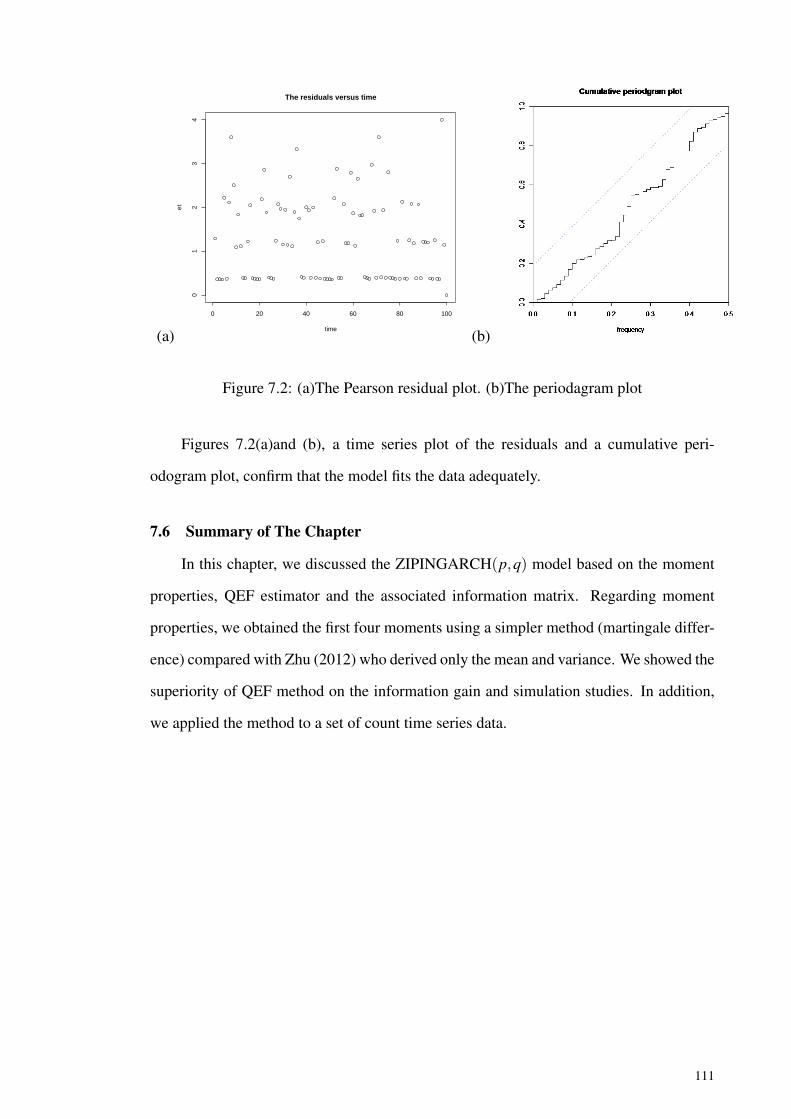
(a)
0 20 40 60 80 100
01
23
4
The residuals versus time
time
et
(b)
Figure 7.2: (a)The Pearson residual plot. (b)The periodagram plot
Figures 7.2(a)and (b), a time series plot of the residuals and a cumulative peri-
odogram plot, confirm that the model fits the data adequately.
7.6 Summary of The Chapter
In this chapter, we discussed the ZIPINGARCH(p,q) model based on the moment
properties, QEF estimator and the associated information matrix. Regarding moment
properties, we obtained the first four moments using a simpler method (martingale differ-
ence) compared with Zhu (2012) who derived only the mean and variance. We showed the
superiority of QEF method on the information gain and simulation studies. In addition,
we applied the method to a set of count time series data.
111

CHAPTER 8
CONCLUSION
This chapter provides a short summary of the main results presented in the thesis and
discuss important challenges for future research.
8.1 Summary of The Study
This study focused on integer-valued time series models analogue of the general-
ized autoregressive conditional heteroscedastic, GARCH(p,q), with the conditional dis-
tribution following the integer-valued distributions, Poisson, negative binomial and zero-
inflated Poisson. The models are known as INGARCH(p,q), NBINGARCH(p,q) and
ZIPINGARCH(p,q) models respectively.
Firstly, we derived the moments of the models up to order four using martingale dif-
ference. The first and second moment properties are available in literatures but not for the
third and fourth moment properties which are skewness and kurtosis. Zhu (2012) stated
that the derivation of the unconditional distributions are complicated for these models
and needs further investigation. Therefore, we found a general closed form expressions
of skewness and kurtosis for these models in closed form expression. The theorem and
derivation of general form of skewness and kurtosis of these models were shown in Chap-
ter 3. In Chapter 5, 6 and 7, we obtained the skewness and kurtosis for each model by
finding the skewness and kurtosis of each martingale difference of the model. This finding
is very important in line with the opinion of Patton (2004) who stated that the knowledge
of these higher moments, skewness and kurtosis will make a significant better forecast on
assets, both statistically and economically.
Secondly, in time series analysis, one of important interest is to have a good param-
eter estimation method. Instead of the traditional MLE we consider the optimal QEF
method proposed by Liang et al. (2011). The theory on QEF method was discussed in
Chapter 4. We also gave some examples for simple integer-valued time series models
based on zero-inflated poisson distribution namely basic zero-inflated Poisson and zero-
112

inflated Poisson regression models. This method of parameter estimation have been stud-
ied and applied into continuous time series models, for example random coefficient au-
toregressive (RCA) model by Thavaneswaran et al. (2015) and autoregressive conditional
duration (ACD) model (see Ng et al. (2015)). However, there were no study using QEF
method on the integer-valued time series model. Therefore, in this research, we studied
and discussed the methodology on integer-valued time series models to see its perfor-
mance compared to other parameter estimations methods. Here, we derived the optimal
QEF functions and their information matrices for each process. Theoretically, we com-
pared the information gain by QEF method with each component of estimating functions.
We conducted simulation studies to see the performance of QEF method compared to
other estimation methods namely MLE and EF methods via R-cran programming. From
the results obtained, we saw that the QEF estimators outperform MLE, LS and EF es-
timators in almost all cases especially for near non-stationary cases. Therefore, we can
conclude that, the QEF estimator can be an efficient alternative method for parameter
estimation on these models.
Lastly, we applied the methodology on real-world data set. We fitted these models
(INGARCH(p,q), NBINGARCH(p,q) and ZIPINGARCH(p,q) models) in Chapter 5,
6 and 7 and estimated parameters using MLE, LS/EF and QEF. In each case, the model
fit was examined by the AIC, BIC methods, Pearson residuals and their plots, Ljung-Box
tests, and cumulative periodogram tests. In all cases we found that the models considered
fitted well to the data sets.
From this study, we concluded that the findings are very important and will be benefi-
cial to the statistical area. This research can adds more knowledge to the area of modeling
integer-valued time series data and their properties at the higher order up to order four.
The new methods of deriving moments using the martingale differences and other simpler
methods will be useful for other statistical researchers.
8.2 Further Research
In this section, we discuss the possibilities for further research on the work presented
in this thesis. Some suggestions are given as follows:
113

1. Extend the theory on zero-inflated negative binomial GARCH (ZINBINGARCH(p,q))
model.
From the research done, we can extend the moment properties to ZINBINGARCH(p,q)
model. The moments properties for both conditional and unconditional for this model are
quite complicate because of the complex expressions for the factorial cumulant. Due to
this reason, it deserve a further investigation to simplify the derivation on the moments
for conditional distribution of ZINBINGARCH(p,q) model and then plug in the result
obtained into our Theorem 1 and Theorem 2 to have the unconditional moment properties
of unconditional distribution of ZINBINGARCH(p,q) model.
2. Apply the QEF estimator on other integer-valued time series models.
In this research, we apply the QEF method on the class of integer-valued GARCH(p,q)
models. We show that the estimator performs well compared to MLE and EF methods.
Hence, the method should be extended for other class of integer-valued time series mod-
els, such as INAR(p) and etc.
3. Extend the use of higher moment properties of INGARCH(p,q) family especially in
forecasting the volatility of the models.
Forecasting plays an important part in both linear and nonlinear time series cases. Tha-
vaneswaran et al. (2005) mentioned that the kurtosis of a time series model can be used
to forecast the error variance while Patton (2004) highlighted that significant of higher
moments, namely skewness and kurtosis, can lead to better forecasts. Therefore, it is pos-
sible, we can extend the use of skewness and kurtosis of the models to forecast volatility.
114

REFERENCES
Abraham, . L. J., B. (2009). Statistical methods for forecasting (Vol. 234). New York,USA: John Wiley & Sons.
Allen, D., Ng, K., & Peiris, S. (2013a). The efficient modelling of high frequencytransaction data: A new application of estimating functions in financial economics.Economics Letters, 120(1), 117–122.
Allen, D., Ng, K., & Peiris, S. (2013b). Estimating and simulating weibull models ofrisk or price durations: An application to acd models. The North American Journal ofEconomics and Finance, 25, 214–225.
Al-Osh, M. A., & Alzaid, A. A. (1987). First-order integer-valued autoregressive (inar(1)) process. Journal of Time Series Analysis, 8(3), 261–275.
Aly, E.-E. A., & Bouzar, N. (1994). On some integer-valued autoregressive movingaverage models. Journal of multivariate analysis, 50(1), 132–151.
Bahadur, R. R. (1958). Examples of inconsistency of maximum likelihood estimates.Sankhya: The Indian Journal of Statistics, 20(3/4), 207–210.
Baillie, R. T., & Bollerslev, T. (2002). The message in daily exchange rates: Aconditional-variance tale. Journal of Business & Economic Statistics, 20(1), 60–68.
Baksh, M. F., Böhning, D., & Lerdsuwansri, R. (2011). An extension of an over-dispersion test for count data. Computational Statistics & Data Analysis, 55(1), 466–474.
Bera, A. K., & Bilias, Y. (2002). The mm, me, ml, el, ef and gmm approaches toestimation: A synthesis. Journal of Econometrics, 107(1), 51–86.
Bera, A. K., Bilias, Y., & Simlai, P. (2006). Estimating functions and equations: An essayon historical developments with applications to econometrics. Palgrave Handbook ofEconometrics, 1, 427–476.
Bollerslev, T. (1986). Generalized autoregressive conditional heteroskedasticity. Journalof econometrics, 31(3), 307–327.
Brockwell, P. J., & Davis, R. A. (1991). Time series: Theory and methods. SpringerSeries in Statistics. Springer-V erlag,, 1(99), 1.
Brockwell, P. J., & Davis, R. A. (2013). Time series: Theory and methods. Colorada,USA: Springer Science & Business Media.
Cameron, A. C., & Trivedi, P. K. (2001). Essentials of count data regression. Blackwell,Oxford (U.K.): Blackwell Publishing Ltd.
Carvalho, A. X., & Tanner, M. A. (2007). Modelling nonlinear count time series withlocal mixtures of poisson autoregressions. Computational statistics & data analysis,51(11), 5266–5294.
Casella, G., & Berger, R. L. (2002). Statistical inference (Vol. 2). Florida, USA: DuxburyPacific Grove, CA.
Chandra, S. A., & Taniguchi, M. (2001). Estimating functions for nonlinear time seriesmodels. Annals of the Institute of Statistical Mathematics, 53(1), 125–141.
Crowder, M. (1987). On linear and quadratic estimating functions. Biometrika, 74(3),591–597.
Davis, R. A., Holan, S. H., Lund, R., & Ravishanker, N. (2016). Handbook of discrete-valued time series. New York: CRC Press.
Davis, R. A., & Wu, R. (2009). A negative binomial model for time series of counts.Biometrika, 96(3), 735–749.
115

Diebold, F. X. (2004). The nobel memorial prize for robert f. engle. The ScandinavianJournal of Economics, 106(2), 165–185.
Durbin, J. (1960). Estimation of parameters in time-series regression models. Journal ofthe Royal Statistical Society. Series B (Methodological), 22(1), 139–153.
Engle, R. F. (1982). Autoregressive conditional heteroscedasticity with estimates ofthe variance of united kingdom inflation. Econometrica: Journal of the EconometricSociety, 50(4), 987–1007.
Engle, R. F., & Bollerslev, T. (1986). Modelling the persistence of conditional variances.Econometric reviews, 5(1), 1–50.
Engle, R. F., & Ng, V. K. (1993). Measuring and testing the impact of news on volatility.The journal of finance, 48(5), 1749–1778.
Feigin, P. D., Gould, P., Martin, G. M., & Snyder, R. D. (2008). Feasible parameterregions for alternative discrete state space models. Statistics & Probability Letters,78(17), 2963–2970.
Feller, W. (1943). On a general class of" contagious" distributions. The Annals ofmathematical statistics, 14(4), 389–400.
Ferland, R., Latour, A., & Oraichi, D. (2006). Integer-valued garch process. Journal ofTime Series Analysis, 27(6), 923–942.
Fisher, R. A. (1935). The fiducial argument in statistical inference. Annals of eugenics,6(4), 391–398.
Fokianos, K., Rahbek, A., & Tjøstheim, D. (2009). Poisson autoregression. Journal ofthe American Statistical Association, 104(488), 1430–1439.
Franke, J. (2010). Weak dependence of functional ingarch processes. Technische Univer-sität Kaiserslautern, Fachbereich Mathematik.
Ghahramani, M., & Thavaneswaran, A. (2009). Combining estimating functions forvolatility. Journal of Statistical Planning and Inference, 139(4), 1449–1461.
Godambe, V. P. (1960). An optimum property of regular maximum likelihood estimation.The Annals of Mathematical Statistics, 31(4), 1208–1211.
Godambe, V. P. (1985). The foundations of finite sample estimation in stochastic pro-cesses. Biometrika, 72(2), 419–428.
Godambe, V. P., & Heyde, C. C. (2010). Quasi-likelihood and optimal estimation. InSelected works of cc heyde (Vol. 55, pp. 386–399). Springer.
Gray, S. F. (1996). Modeling the conditional distribution of interest rates as a regime-switching process. Journal of Financial Economics, 42(1), 27–62.
Harvey, A., & Fernandes, C. (1989). Time series models for insurance claims. Journalof the Institute of Actuaries, 116(3), 513–528.
Houseman, E. A., Coull, B. A., & Shine, J. P. (2006). A nonstationary negative bino-mial time series with time-dependent covariates: Enterococcus counts in boston harbor.Journal of the American Statistical Association, 101(476), 1365–1376.
Johansson, P. (1996). Speed limitation and motorway casualties: A time series count dataregression approach. Accident Analysis & Prevention, 28(1), 73–87.
Johnson, N. L., Kemp, A. W., & Kotz, S. (2005). Univariate discrete distributions(Vol. 444). Canada: John Wiley & Sons.
Jung, R. C., Ronning, G., & Tremayne, A. R. (2005). Estimation in conditional first orderautoregression with discrete support. Statistical papers, 46(2), 195–224.
116

Kachour, M. (2009). p-order rounded integer-valued autoregressive (rinar (p)) process.Journal of Time Series Analysis, 30(4), 417-448.
Kedem, B., & Fokianos, K. (2005). Regression models for time series analysis (Vol. 488).USA: John Wiley & Sons.
Kharrati-Kopaei, M., & Faghih, H. (2011). Inferences for the inflation parameter in thezip distributions: The method of moments. Statistical Methodology, 8(4), 377–388.
Kimball, B. F., et al. (1946). Sufficient statistical estimation functions for the parametersof the distribution of maximum values. The Annals of Mathematical Statistics, 17(3),299–309.
Lambert, D. (1992). Zero-inflated poisson regression, with an application to defects inmanufacturing. Technometrics, 34(1), 1–14.
Le Cam, L. (1990). Maximum likelihood: An introduction. International StatisticalReview/Revue Internationale de Statistique, 58, 153–171.
Lehmann, E. L., & Casella, G. (1991). Theory of point estimation. USA: Wadsworth &Brooks/Cole Advanced Books & Software.
Li, G., Haining, R., Richardson, S., & Best, N. (2014). Space–time variability in burglaryrisk: A bayesian spatio-temporal modelling approach. Spatial Statistics, 9, 180–191.
Liang, Y., Thavaneswaran, A., & Abraham, B. (2011). Joint estimation using quadraticestimating function. Journal of Probability and Statistics, 2011.
Lim, H. K., Li, W. K., & Philip, L. (2014). Zero-inflated poisson regression mixturemodel. Computational Statistics & Data Analysis, 71, 151–158.
Lukusa, T. M., Lee, S.-M., & Li, C.-S. (2015). Semiparametric estimation of a zero-inflated poisson regression model with missing covariates. Metrika, 79(4), 457–483.
MacDonald, I. L., & Zucchini, W. (1997). Hidden markov and other models for discrete-valued time series (Vol. 110). USA: CRC Press.
McKenzie, E. (1985). Some simple models for discrete variate time series. Water Re-sources Bulletins, 21, 645-650.
Merkouris, T., et al. (2007). Transform martingale estimating functions. The Annals ofStatistics, 35(5), 1975–2000.
Mullahy, J. (1997). Heterogeneity, excess zeros, and the structure of count data models.Journal of Applied Econometrics, 12(3), 337–350.
Nanjundan, G., & Naika, T. R. (2012). Asymptotic comparison of method of momentsestimators and maximum likelihood estimators of parameters in zero-inflated poissonmodel. Applied mathematics, 3(06), 610.
Nastic, A. S., Ristic, M. M., & Bakouch, H. S. (2012). A combined geometric inar (p)model based on negative binomial thinning. Mathematical and Computer Modelling,55(5), 1665–1672.
Nelson, D. B. (1991). Conditional heteroskedasticity in asset returns: A new approach.Econometrica: Journal of the Econometric Society, 59(2), 347–370.
Neyman, J. (1939). On a new class of" contagious" distributions, applicable in entomol-ogy and bacteriology. The Annals of Mathematical Statistics, 10(1), 35–57.
Ng, K. H., & Peiris, S. (2013). Modelling high frequency transaction data in financialeconomics: A comparative study based on simulations. Economic Computation andEconomic Cybernetics Studies and Research, 47(2), 189–202.
Ng, K. H., Peiris, S., & Gerlach, R. (2014). Estimation and forecasting with logarithmicautoregressive conditional duration models: A comparative study with an application.Expert Systems with Applications, 41(7), 3323–3332.
117
Ng, K. H., Shelton, P., Thavaneswaran, A., & Ng, K.-H. (2015). Modelling the risk orprice durations in financial markets: Quadratic estimating functions and applications.Economic Computation & Economic Cybernetics Studies & Research, 49(1).
Patton, A. J. (2004). On the out-of-sample importance of skewness and asymmetricdependence for asset allocation. Journal of Financial Econometrics, 2(1), 130–168.
Pedeli, X., & Karlis, D. (2011). A bivariate inar (1) process with application. Statisticalmodelling, 11(4), 325–349.
Puig, P., & Valero, J. (2006). Count data distributions: Some characterizations withapplications. Journal of the American Statistical Association, 101(473), 332–340.
Sellers, K. F., & Raim, A. (2016). A flexible zero-inflated model to address data disper-sion. Computational Statistics & Data Analysis, 99, 68–80.
Sentana, E. (1995). Quadratic arch models. The Review of Economic Studies, 62(4),639–661.
Spiegel, M. (1999). Schaum’s mathematical handbook of formulas and tables. USA:McGraw-Hill Osborne Media.
Staub, K. E., & Winkelmann, R. (2013). Consistent estimation of zero-inflated countmodels. Health economics, 22(6), 673–686.
Thavaneswaran, A., & Abraham, B. (1988). Estimation for nonlinear time series modelsusing estimating equations. Journal of Time Series Analysis, 9(1), 99–108.
Thavaneswaran, A., Appadoo, S. S., & Samanta, M. (2005). Random coefficient garchmodels. Mathematical and Computer Modelling, 41(6), 723–733.
Thavaneswaran, A., Liang, Y., & Frank, J. (2012). Inference for random coefficientvolatility models. Statistics & Probability Letters, 82(12), 2086–2090.
Thavaneswaran, A., Ravishanker, N., & Liang, Y. (2015). Generalized duration modelsand optimal estimation using estimating functions. Annals of the Institute of StatisticalMathematics, 67(1), 129–156.
Tsay, R. S. (2014). An introduction to analysis of financial data with r. Chicago, USA:John Wiley & Sons.
Vinod, H. (1997). Using godambe-durbin estimating functions in econometrics. LectureNotes-Monograph Series, 32, 215–237.
Wang, P. (2001). Markov zero-inflated poisson regression models for a time series ofcounts with excess zeros. Journal of Applied Statistics, 28(5), 623–632.
Weiß, C. H. (2010). The inarch (1) model for overdispersed time series of counts. Com-munications in Statistics-Simulation and Computation, 39(6), 1269–1291.
Weiß, C. H. (2013). Integer-valued autoregressive models for counts showing underdis-persion. Journal of Applied Statistics, 40(9), 1931–1948.
Wurtz, D., Chalabi, Y., & Luksan, L. (2009). Parameter estimation of arma modelswith garch/aparch errors an r and splus software implementation. Journal of StatisticalSoftware, forthcoming. Retrieved from http://www.jstatsoft.org/ doi: doi=10.1.1.693.9113
Yang, M. (2012). Statistical models for count time series with excess zeros.
Yang, M., Zamba, G. K., Cavanaugh, J. E., & Yang, M. M. (2014). Package zim.
Yau, K. K., Lee, A. H., & Carrivick, P. J. (2004). Modeling zero-inflated count series withapplication to occupational health. Computer Methods and Programs in Biomedicine,74(1), 47–52.
118

Zeger, S. L. (1988). A regression model for time series of counts. Biometrika, 75(4),621–629.
Zhu, F. (2011). A negative binomial integer-valued garch model. Journal of Time SeriesAnalysis, 32(1), 54–67.
Zhu, F. (2012). Zero-inflated poisson and negative binomial integer-valued garch models.Journal of Statistical Planning and Inference, 142(4), 826–839.
119

APPENDIX A
THEOREM OPTIMAL EF FOR THE DEPENDENT CASE
From the Theorem 2.3.1, we notice that to minimize g∗, the value of numerator
should be minimized and the denominator to be maximized. From the numerator, we
have
E[g2 (X : θ)
]= E
[n
∑t=1
a2t−1E
(h2
t |ℑXt−1)]
. (A.1)
On the other hand, for denominator, we have
E[
dg(Xθ)dθ
]2
=
E
n
∑t=1
(at−1E
(∂ht
∂θ|ℑX
t−1
))2
. (A.2)
For the optimal EF, we have
E[g∗2 (X : θ)
]= E
[n
∑t=1
a∗2t−1E
(h2
t |ℑXt−1)]
. (A.3)
where a∗t−1 =E[
dhtdθ |ℑX
t−1
]E[h2
t |ℑXt−1]
, therefore, equation (A.3) can be rewritten in following form:
E[g∗2 (X : θ)
]= E
n
∑t=1
E[
dhtdθ |ℑ
Xt−1
]E[h2
t |ℑXt−1]2
E[h2
t |ℑXt−1] .
On the other hand, using (A.2), its denominator is given in this way:
E[
dg(X ;θ)dθ
]2
=
E
n
∑t=1
(a∗t−1E
(∂ht
∂θ|ℑX
t−1
))2
=
at−1
E[h2
t |ℑXt−1]
E[h2
t |ℑXt−1]E(
∂ht
∂θ|ℑX
t−1
),
2
. (A.4)
120

Using Cauchy-Schwarz inequality, one knows that:
E[
dg(X ;θ)dθ
]2
=
[E
n
∑t=1
at−1
E[h2
t |ℑXt−1]
E[h2
t |ℑXt−1]E(
∂ht
∂θ|ℑX
t−1
)]2
≤ E
n
∑t=1
a2t−1E
[h2
t |ℑXt−1]
E
n
∑t=1
E[
dg(Xθ)dθ
]2
E[h2
t |ℑXt−1]
= E(g2) E
[dg∗dθ
]2
E (g∗2).
Therefore, we can conclude that
E(g∗2)[
E(
dg∗dθ
)]2 ≤E(g2)[
E(
dgdθ
)]2 .
Hence, the theorem is proven.
121

APPENDIX B
FEIGIN’S THEOREM
By equation (3.21) and Theorem (3.5.1), the Laplace transform of the stationary distribu-
tion of Xt satisfies LX(u) = exp−λ ∑∞
k=0 g(k) (1− e−u)
for u ≥ 0.
Proof:
The Laplace transform for λt is Lλt (υ) where
Lλt (υ) = exp(−υλ )Lλt−1g(υ ;δ ,α). (B.1)
Let g(υ ;δ ,α) = g(υ), therefore Lλt (υ) = exp(−υλ )Lλt−1g(υ). Since t always positive,
we have, Lλ0(υ) = exp(−υλ ), then,
Lλ1(υ) = exp(−υλ )Lλ0 (g(υ)) ,
= exp(−υλ )exp(−g(υ)λ ) ,
Lλ2(υ) = exp(−υλ )Lλ1 (g(υ)) ,
= exp(−υλ ) [exp(−g(υ)λ )exp(−g(g(υ))λ )] ,
Lλ3(υ) = exp(−υλ )Lλ2 (g(υ)) ,
= exp(−υλ ) [exp(−g(υ)λ )exp(−g(g(υ))λ )exp(−g(g(g(υ)))λ )] ,... (B.2)
Lλ∞ = = exp(−υλ ) [exp(−g(υ)λ )exp(−g(g(υ))λ )exp(−g(g(g(υ)))λ ) . . .]
= exp(−λ
υ +g1(υ)+g2(υ)+ . . .)
.
Let g0(υ) = υ , then
Lλ∞ = exp(−λ
g0(υ +g1(υ)+g2(υ)+ . . .)
= exp
(−λ
∞
∑k=0
g(k)(υ)
). (B.3)
Therefore, the theorem is proven.
122
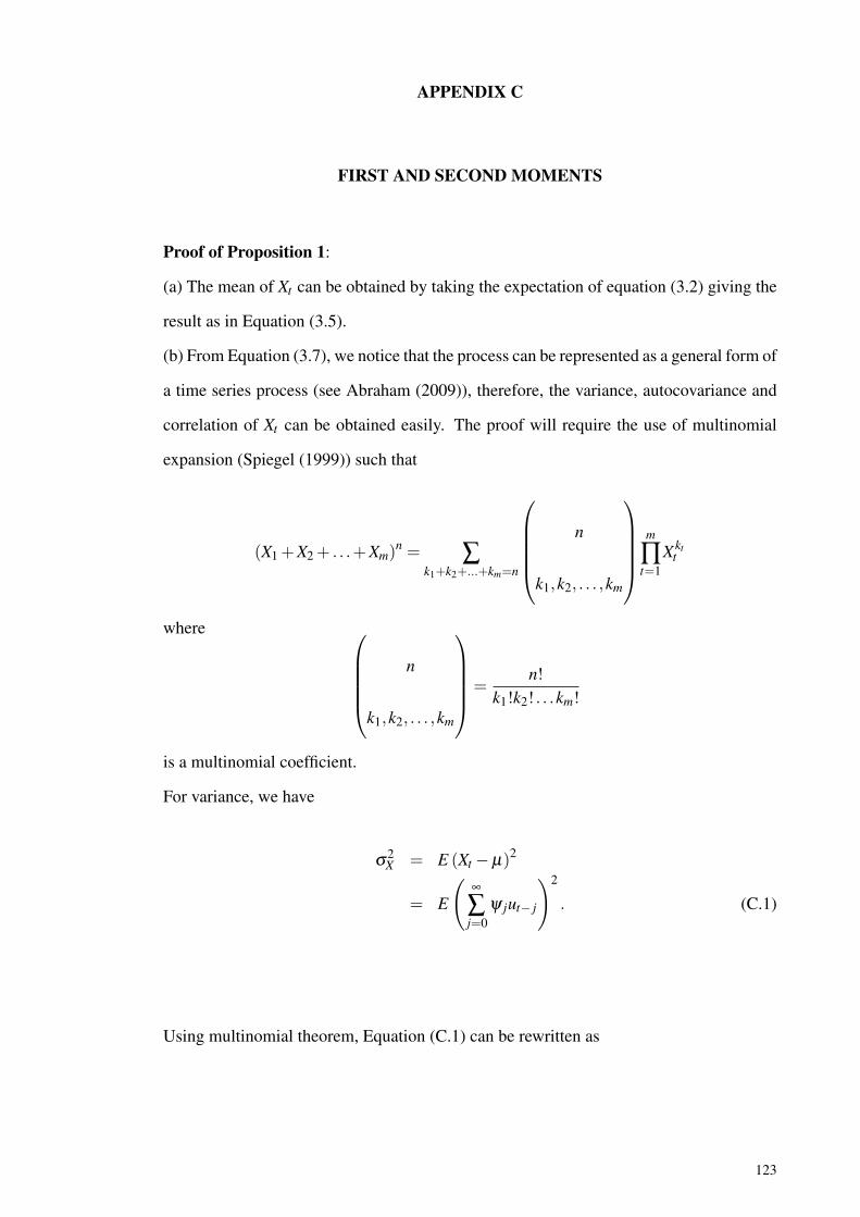
APPENDIX C
FIRST AND SECOND MOMENTS
Proof of Proposition 1:
(a) The mean of Xt can be obtained by taking the expectation of equation (3.2) giving the
result as in Equation (3.5).
(b) From Equation (3.7), we notice that the process can be represented as a general form of
a time series process (see Abraham (2009)), therefore, the variance, autocovariance and
correlation of Xt can be obtained easily. The proof will require the use of multinomial
expansion (Spiegel (1999)) such that
(X1 +X2 + . . .+Xm)n = ∑
k1+k2+...+km=n
n
k1,k2, . . . ,km
m
∏t=1
Xktt
where n
k1,k2, . . . ,km
=n!
k1!k2! . . .km!
is a multinomial coefficient.
For variance, we have
σ2X = E (Xt −µ)2
= E
(∞
∑j=0
ψ jut− j
)2
. (C.1)
Using multinomial theorem, Equation (C.1) can be rewritten as
123

σ2X = E
2
2,0,0, . . .
∑∞j=0 ψ2
j u2t− j
+E
2
1,1,0, . . .
∑∞j=0 ψ jut− j
,
=
2
2,0,0, . . .
∑∞j=0 ψ2
j E[u2
t− j
]+
2
1,1,0, . . .
∑∞j=0 ψ jE
[ut− j
],
=∞
∑j=0
ψ2j σ2
u +∞
∑j=0
ψ j (0)
=∞
∑j=0
ψ2j σ2
u .
(c) The autocovariance can be defined as
γXk = E (Xt −µ)(Xt+k −µ)
= E
[(∞
∑j=0
ψ jut− j
)(∞
∑j=0
ψ j+kut+k− j
)]. (C.2)
The right hand side of (C.2) can be written as
E [(ψ0ut +ψ1ut−1 +ψ2ut−2 + . . .)(ψ0ut+k +ψ1ut+k−1 +ψ2ut+k−2 + . . .)] ,
where the expansion is
124

γXk = E
ψ0utψ0ut+k +ψ0utψ1ut+k−1
+ψ0utψ2ut+k−2 + . . .+ψ0utψkut + . . .+
ψ1ut−1ψ0ut+k +ψ1ut−1ψ1ut+k−1+
ψ1ut−1ψ2ut+k−2 + . . .++ψ1ut−1ψk+1ut−1 + . . .
ψ2ut−2ψ0ut+k +ψ2ut−2ψ1ut+k−1+
ψ2ut−2ψ2ut+k−2 + . . .++ψ2ut−2ψk+2ut−2 + . . .
+ . . . . . .+ . . . . . .+ . . . . . .
.
(C.3)
Rearrange (C.3), we have
γXk = E
ψ0utψ0ut+k +ψ1ut−1ψ1ut+k−1+
ψ2ut−2ψ2ut+k−2 + . . .+ . . .+
ψ0utψ1ut+k−1 +ψ0utψ2ut+k−2 + . . .
ψ1ut−1ψ0ut+k +ψ1ut−1ψ2ut+k−2 + . . .+
ψ0utψkut +ψ1ut−1ψk+1ut−1+
+ψ2ut−2ψk+2ut−2 + . . .+ . . .
.
Hence, we have
γXk = E
∑∞
j=0 ψ2j ut− jut+k− j +∑∞
j=0 ψ jψk+ ju2t− j
+∑∞j=0 ∑∞
i= j ψ jut− jψiut+k−i
.(C.4)
125

Then, taking the expectation on the right hand side, the autocovariance is given by
γXk =
∞
∑j=0
ψ2j E(ut− j
)E(ut+k− j
)+
∞
∑j=0
ψ jψk+ jE(u2
t− j)
+∞
∑j=0
∞
∑i= j
ψ jE(ut− j
)ψiE (ut+k−i)
=∞
∑j=0
ψ2j (0)(0)+
∞
∑j=0
ψ jψk+ jσ2u
+∞
∑j=0
∞
∑i= j
ψ j (0)ψi (0)
=∞
∑j=0
ψ jψk+ jσ2u .
(d) Lastly for autocorrelation, we substitute the variance in (b) and the autocovariance in
(c) into the autocorrelation formula giving
ρXk =
γX
σ2X,
=σ2
u ∑∞j=0 ψ jψ j+k
σ2u ∑∞
j=0 ψ2j
,
=∑∞
j=0 ψ jψ j+k
∑∞j=0 ψ2
j.
126

APPENDIX D
HIGHER ORDER OF MOMENTS
Proof for Proposition 2:
(a)We first define the expectation of St as E (St) = E (Xt −µ)2 = Var(Xt) = σ2u ∑∞
j=0 ψ2j .
One knows that E(S2
t)= E (Xt −µ)4 = E
(∑∞
j=0 ψ jut− j
)4. By using multinomial expan-
sion, E(S2
t)
is
E(S2
t)
= E
4
4,0,0, . . .
∑∞j=0 ψ4
j u4t− j +
4
3,1,0,0, . . .
∑∞i=0 ∑∞
j=i+1 ψ3i u3
t−iψ jut− j+
4
1,3,0,0, . . .
∑∞i=0 ∑∞
j=i+1 ψiut−iψ3j u3
t− j+
4
2,2,0,0, . . .
∑∞i=0 ∑∞
j=i+1 ψ2i u2
t−iψ2j u2
t− j+
4
2,1,1,0, . . .
∑∞i=0 ∑∞
j=i+1 ∑∞k= j+1 ψ2
i u2t−iψ jut− jψkut−k+
4
1,2,1,0, . . .
∑∞i=0 ∑∞
j=i+1 ∑∞k= j+1 ψiut−iψ2
j u2t− jψkut−k+
4
1,1,2,0, . . .
∑∞i=0 ∑∞
j=i+1 ∑∞k= j+1 ψ2
i u2t−iψ jut− jψ2
k u2t−k+
4
1,1,1,1, . . .
∑∞i=0 ∑∞
j=i+1 ∑∞k= j+1 ∑∞
l=k+1 ψ2i u2
t−iψ jut− jψkut−kψlut−l
,
127

= E
∑∞j=0 ψ4
j u4t− j +4∑∞
i=0 ∑∞j=i+1 ψ3
i u3t−iψ jut− j+
4∑∞i=0 ∑∞
j=i+1 ψiut−iψ3j u3
t− j +6∑∞i=0 ∑∞
j=i+1 ψ2i u2
t−iψ2j u2
t− j+
12∑∞i=0 ∑∞
j=i+1 ∑∞k= j+1 ψ2
i u2t−iψ jut− jψkut−k
+12∑∞i=0 ∑∞
j=i+1 ∑∞k= j+1 ψiut−iψ2
j u2t− jψkut−k
+12∑∞i=0 ∑∞
j=i+1 ∑∞k= j+1 ψiut−iψ jut− jψ2
k u2t−k
+24∑∞i=0 ∑∞
j=i+1 ∑∞k= j+1 ∑∞
l=k+1 ψiut−iψ jut− jψkut−kψlut−l
.
Taking the expectation, we have:
E(S2
t)=
∞
∑j=0
ψ4j E(u4
t− j)+4
∞
∑i=0
∞
∑j=i+1
ψ3i ψ jE
(u3
t−iut− j)
+4∞
∑i=0
∞
∑j=i+1
ψiψ3j E(ut−iu3
t− j)+6
∞
∑i=0
∞
∑j=i+1
ψ2i ψ2
j E(u2
t−iu2t− j)
+12∞
∑i=0
∞
∑j=i+1
∞
∑k= j+1
ψ2i ψ jψkE
(u2
t−iut− jut−k)
+12∞
∑i=0
∞
∑j=i+1
∞
∑k= j+1
ψiψ2j ψkE
(ut−iu2
t− jut−k)
+12∞
∑i=0
∞
∑j=i+1
∞
∑k= j+1
ψiψ jψ2k E(ut−iut− ju2
t−k)
+24∞
∑i=0
∞
∑j=i+1
∞
∑k= j+1
∞
∑l=k+1
ψ2i ψ jψkψlE
(ut−iut− jut−kut−l
)(D.1)
According to Johnson et al. (2005), the kurtosis is given by
K(Xt) =E (Xt −µ)4
[Var(Xt)]2 . (D.2)
This definition implies that the fourth moment of ut can be written as E(u4
t)= K(u)σ4
u
and ut is an uncorrelated series with zero mean, E (ut) = 0, we can simply apply into
Equation (D.1) whereby
E(S2
t)
=∞
∑j=0
ψ4j E(u4
t− j)+4
∞
∑j=i
∞
∑j=i+1
ψ3i ψ jE
(u3
t−i)
E(ut− j
)128

+6∞
∑j=i
∞
∑j=i+1
ψ3i ψ jE
(u2
t−i)
E(u2
t− j),
=∞
∑j=0
ψ4j K(u)σ4
u +6∞
∑i=0
∞
∑j=i+1
ψ2i ψ2
j σ4u . (D.3)
From (D.3), we can reduce 6∑∞i=0 ∑∞
j=i+1 ψ2i ψ2
j to 3(
∑∞j=0 ψ2
j
)2− 3∑∞
j=0 ψ4j . The ex-
pansion come from multinomial expansion for binomial case which is
(∞
∑j=0
ψ j
)2
=∞
∑j=0
2
2,0,0, . . .
ψ2j +
∞
∑i=0
∞
∑j=i+1
2
1,1,0,0, . . .
ψiψ j
=∞
∑j=0
ψ2j +2
∞
∑i=0
∞
∑j=i+1
ψiψ j.
Then, we rearrange to be 2∑∞i=0 ∑∞
j=i+1 ψiψ j =(
∑∞j=0 ψ j
)2−∑∞
j=0 ψ2j . Therefore, for
our case, we will multiply both side with three giving
6∞
∑i=0
∞
∑j=i+1
ψ2i ψ2
j = 3
(2
∞
∑i=0
∞
∑j=i+1
ψ2i ψ2
j
)= 3
( ∞
∑j=0
ψ2j
)2
−∞
∑j=0
ψ4j
.
Thus,
Var (St) = E(S2
t)− [E (St)]
2
=∞
∑j=0
ψ4j K(u)σ4
u +3σ4u
( ∞
∑j=0
ψ2j
)2
−∞
∑j=0
ψ4j
−σ4u
(∞
∑j=0
ψ2j
)2
=(
K(u)−3)
σ4u
∞
∑j=0
ψ4j +2σ4
u
(∞
∑j=0
ψ2j
)2
. (D.4)
(b) On the other hand, the third moment of a process known as skewness is also one of the
important properties of a model. Skewness is a measure of symmetry of a distribution.
If the skewness is positive, the graph is right skewed and vice versa. A distribution with
zero skewness indicates that it is symmetrical. According to Johnson et al. (2005), the
129

skewness is defined as
Γ(X) =E[(Xt −µ)3
][Var(Xt)]
3/2 (D.5)
Since the process Xt can be written in general form, the third moment of Xt is
E (Xt −µ)3 = E
(∞
∑j=0
ψ jut− j
)3
. (D.6)
From the right hand side Equation (D.6), the process can be expanded using multinomial
expansion, therefore:
E
(∞
∑j=0
ψ jut− j
)3
= E
∑∞j=0
3
3,0,0, . . .
ψ3j u3
t− j+
∑∞i=0 ∑∞
j=i+1
3
2,1,0,0, . . .
ψ2i u2
t−iψ jut− j+
∑∞i=0 ∑∞
j=i+1
3
1,2,0,0, . . .
ψiut−iψ2j u2
t− j+
∑∞i=0 ∑∞
j=i+1 ∑∞k= j+1
3
1,1,1,0, . . .
ψiut−iψ jut− jψkut−k
,
= E
∑∞j=0 ψ3
j u3t− j +3∑∞
i=0 ∑∞j=i+1 ψ2
i u2t−iψ jut− j
+3∑∞i=0 ∑∞
j=i+1 ψiut−iψ2j u2
t− j
+6∑∞i=0 ∑∞
j=i+1 ∑∞k= j+1 ψiut−iψ jut− jψkut−k
,
=∞
∑j=0
ψ3j E(u3
t− j)+3
∞
∑i=0
∞
∑j=i+1
ψ2i ψ jE
(ut− ju2
t−i)
130
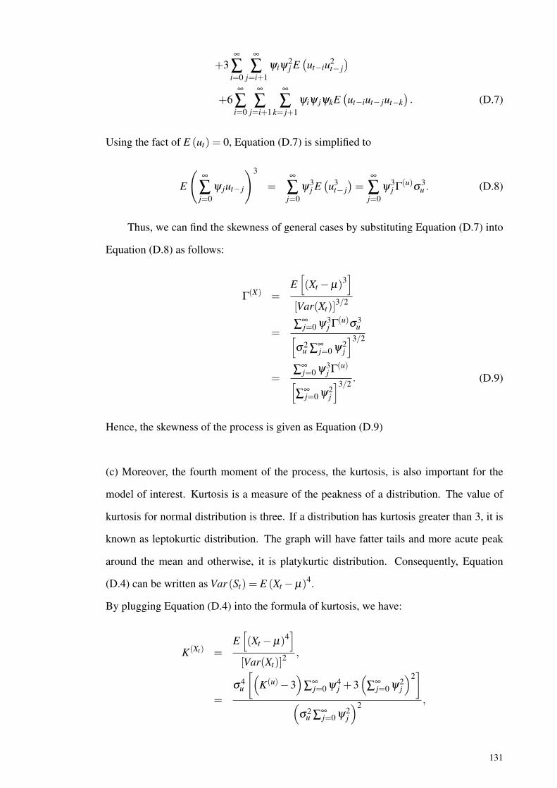
+3∞
∑i=0
∞
∑j=i+1
ψiψ2j E(ut−iu2
t− j)
+6∞
∑i=0
∞
∑j=i+1
∞
∑k= j+1
ψiψ jψkE(ut−iut− jut−k
). (D.7)
Using the fact of E (ut) = 0, Equation (D.7) is simplified to
E
(∞
∑j=0
ψ jut− j
)3
=∞
∑j=0
ψ3j E(u3
t− j)=
∞
∑j=0
ψ3j Γ(u)σ3
u . (D.8)
Thus, we can find the skewness of general cases by substituting Equation (D.7) into
Equation (D.8) as follows:
Γ(X) =E[(Xt −µ)3
][Var(Xt)]
3/2
=∑∞
j=0 ψ3j Γ(u)σ3
u[σ2
u ∑∞j=0 ψ2
j
]3/2
=∑∞
j=0 ψ3j Γ(u)[
∑∞j=0 ψ2
j
]3/2 . (D.9)
Hence, the skewness of the process is given as Equation (D.9)
(c) Moreover, the fourth moment of the process, the kurtosis, is also important for the
model of interest. Kurtosis is a measure of the peakness of a distribution. The value of
kurtosis for normal distribution is three. If a distribution has kurtosis greater than 3, it is
known as leptokurtic distribution. The graph will have fatter tails and more acute peak
around the mean and otherwise, it is platykurtic distribution. Consequently, Equation
(D.4) can be written as Var (St) = E (Xt −µ)4.
By plugging Equation (D.4) into the formula of kurtosis, we have:
K(Xt) =E[(Xt −µ)4
][Var(Xt)]
2 ,
=
σ4u
[(K(u)−3
)∑∞
j=0 ψ4j +3
(∑∞
j=0 ψ2j
)2]
(σ2
u ∑∞j=0 ψ2
j
)2 ,
131

=
(K(u)−3
)∑∞
j=0 ψ4j(
∑∞j=0 ψ2
j
)2 +3. (D.10)
Therefore, given Xt is an integer-valued process and ut is uncorrelated martingale
difference with 0 mean and variance, σ2u , the kurtosis for all non-Gaussian process is
given as Equation (D.10).
(d) For the general representation of the process the autocorrelation is found as ρXtk =
∑∞j=0 ψ jψ j+k
∑∞j=0 ψ2
j(see Abraham (2009)). From Theorem (2), we also pay attention to the corre-
lation of St . Again, using the multinomial expansion, it is easily seen that
St = (Xt −µ)2 =
(∞
∑j=0
ψ jut− j
)2
=∞
∑j=0
ψ2j u2
t− j +2∞
∑i=0
∞
∑j=i+1
ψiui−1ψ jut− j,
and
St+k = (Xt+k −µ)2 =
(∞
∑j=0
ψ jut+k− j
)2
=∞
∑j=0
ψ2j u2
t+k− j +2∞
∑i=0
∞
∑j=i+1
ψiut+k−iψ jut+k− j.
The covariance is defined as cov(XtXt+k)=E [Xt −E (Xt)] [Xt+k −E (Xt+k)] . Using this
definition, we can simplify it as cov(XtXt+k) = E (XtXt+k)−E (Xt)E (Xt+k) .
Therefore, the covariance for St can be simplified as cov(St)=E (StSt+k)−E (St)E (St+k).
We may find E (StSt+k) as below:
E (StSt+k) = E
(
∑∞j=0 ψ2
j u2t− j +2∑∞
i=0 ∑∞j=i+1 ψiut−iψ jut− j
)×
(∑∞
j=0 ψ2j u2
t+k− j +2∑∞i=0 ∑∞
j=i+1 ψiut+k−iψ jut+k− j
) . (D.11)
We expand the multiplication in Equation (D.11) giving:
E (StSt+k) = E
[(∞
∑j=0
ψ2j u2
t− j
)(∞
∑j=0
ψ2j u2
t+k− j
)]
+2E
[(∞
∑j=0
ψ2j u2
t− j
)(∞
∑i=0
∞
∑j=i+1
ψiut+k−iψ jut+k− j
)]
+2E
[(∞
∑j=0
ψ2j u2
t+k− j
)(∞
∑i=0
∞
∑j=i+1
ψiut−iψ jut− j
)]132

+4E
[(∞
∑i=0
∞
∑j=i+1
ψiut−iψ jut− j
)(∞
∑i=0
∞
∑j=i+1
ψiut+k−iψ jut+k− j
)].
(D.12)
Then, we expand the multiplication for each part of (D.12) whereby the Equation
E
[(∞
∑j=0
ψ2j u2
t− j
)(∞
∑j=0
ψ2j u2
t+k− j
)],
can be written as
E[(
ψ20 u2
t +ψ21 u2
t−1 +ψ22 u2
t−2 + . . .)(
ψ20 u2
t+k +ψ21 u2
t+k−1 +ψ22 u2
t+k−2 + . . .)],
giving
E
(
∑∞j=0 ψ2
j u2t− j
)×(
∑∞j=0 ψ2
j u2t+k− j
)= E
ψ20 u2
t ψ20 u2
t+k +ψ20 u2
t ψ21 u2
t+k−1+
ψ20 u2
t ψ22 u2
t+k−2 + . . .+ψ20 u2
t ψ2k u2
t + . . .+
ψ21 u2
t−1ψ20 u2
t+k +ψ21 u2
t−1ψ21 u2
t+k−1+
ψ21 u2
t−1ψ22 u2
t+k−2 + . . .+ψ21 u2
t−1ψ2k+1u2
t−1 + . . .
ψ22 u2
t−2ψ20 u2
t+k +ψ22 u2
t−2ψ21 u2
t+k−1+
ψ22 u2
t−2ψ22 u2
t+k−2 + . . .+ψ22 u2
t−2ψ2k+2u2
t−2 + . . .
+ . . . . . .+ . . . . . .+ . . . . . .
.
133
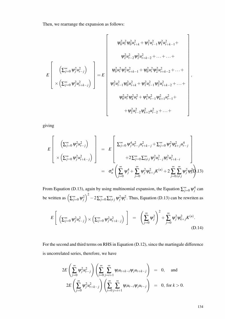
Then, we rearrange the expansion as follows:
E
(
∑∞j=0 ψ2
j u2t− j
)×(
∑∞j=0 ψ2
j u2t+k− j
)= E
ψ20 u2
t ψ20 u2
t+k +ψ21 u2
t−1ψ21 u2
t+k−1+
ψ22 u2
t−2ψ22 u2
t+k−2 + . . .+ . . .+
ψ20 u2
t ψ21 u2
t+k−1 +ψ20 u2
t ψ22 u2
t+k−2 + . . .+
ψ21 u2
t−1ψ20 u2
t+k +ψ21 u2
t−1ψ22 u2
t+k−2 + . . .+
ψ20 u2
t ψ2k u2
t +ψ21 u2
t−1ψ2k+1u2
t−1+
+ψ22 u2
t−2ψ2k+2u2
t−2 + . . .+
,
giving
E
(
∑∞j=0 ψ2
j u2t− j
)×(
∑∞j=0 ψ2
j u2t+k− j
) = E
∑∞
j=0 ψ4j u2
t− ju2t+k− j +∑∞
j=0 ψ2j ψ2
k+ ju4t− j
+2∑∞j=0 ∑∞
i= j ψ2j u2
t− jψ2i u2
t+k−i
= σ4
u
(∞
∑j=0
ψ4j +
∞
∑j=0
ψ2j ψ2
k+ jK(u)+2
∞
∑j=0
∞
∑i = j
ψ2j ψ2
i
).(D.13)
From Equation (D.13), again by using multinomial expansion, the Equation ∑∞j=0 ψ4
j can
be written as(
∑∞j=0 ψ2
j
)2−2∑∞
j=0 ∑∞i = j ψ2
j ψ2i . Thus, Equation (D.13) can be rewriten as
E
[ (∑∞
j=0 ψ2j u2
t− j
)×(
∑∞j=0 ψ2
j u2t+k− j
) ]=
(∞
∑j=0
ψ2j
)2
+∞
∑j=0
ψ2j ψ2
k+ jK(u).
(D.14)
For the second and third terms on RHS in Equation (D.12), since the martingale difference
is uncorrelated series, therefore, we have
2E
(∞
∑j=0
ψ2j u2
t− j
)(∞
∑i=0
∞
∑j=i+1
ψiut+k−iψ jut+k− j
)= 0, and
2E
(∞
∑j=0
ψ2j u2
t+k− j
)(∞
∑i=0
∞
∑j=i+1
ψiut−iψ jut− j
)= 0, for k > 0.
134
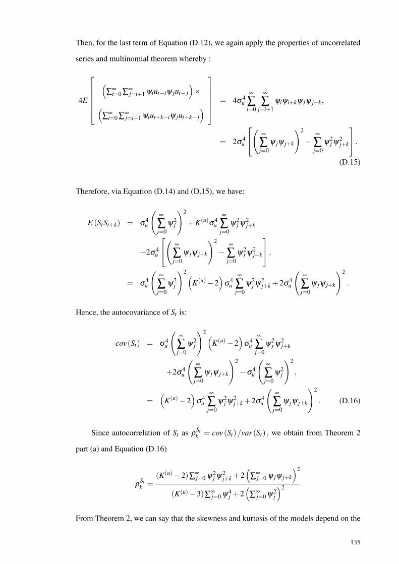
Then, for the last term of Equation (D.12), we again apply the properties of uncorrelated
series and multinomial theorem whereby :
4E
(
∑∞i=0 ∑∞
j=i+1 ψiut−iψ jut− j
)×
(∑∞
i=0 ∑∞j=i+1 ψiut+k−iψ jut+k− j
) = 4σ4
u
∞
∑i=0
∞
∑j=i+1
ψiψi+kψ jψ j+k,
= 2σ4u
( ∞
∑j=0
ψ jψ j+k
)2
−∞
∑j=0
ψ2j ψ2
j+k
.(D.15)
Therefore, via Equation (D.14) and (D.15), we have:
E (StSt+k) = σ4u
(∞
∑j=0
ψ2j
)2
+K(u)σ4u
∞
∑j=0
ψ2j ψ2
j+k
+2σ4u
( ∞
∑j=0
ψ jψ j+k
)2
−∞
∑j=0
ψ2j ψ2
j+k
,= σ4
u
(∞
∑j=0
ψ2j
)2(K(u)−2
)σ4
u
∞
∑j=0
ψ2j ψ2
j+k +2σ4u
(∞
∑j=0
ψ jψ j+k
)2
.
Hence, the autocovariance of St is:
cov(St) = σ4u
(∞
∑j=0
ψ2j
)2(K(u)−2
)σ4
u
∞
∑j=0
ψ2j ψ2
j+k
+2σ4u
(∞
∑j=0
ψ jψ j+k
)2
−σ4u
(∞
∑j=0
ψ2j
)2
,
=(
K(u)−2)
σ4u
∞
∑j=0
ψ2j ψ2
j+k +2σ4u
(∞
∑j=0
ψ jψ j+k
)2
. (D.16)
Since autocorrelation of St as ρStk = cov(St)/var (St) , we obtain from Theorem 2
part (a) and Equation (D.16)
ρStk =
(K(u)−2)∑∞j=0 ψ2
j ψ2j+k +2
(∑∞
j=0 ψ jψ j+k
)2
(K(u)−3)∑∞j=0 ψ4
j +2(
∑∞j=0 ψ2
j
)2
From Theorem 2, we can say that the skewness and kurtosis of the models depend on the
135

skewness and kurtosis of ut such Γ(u) and K(u) and also the weight ψ j.
136
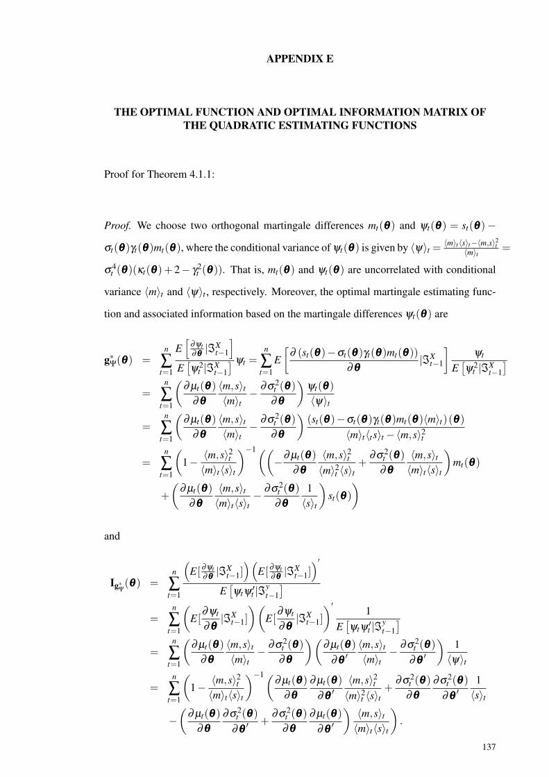
APPENDIX E
THE OPTIMAL FUNCTION AND OPTIMAL INFORMATION MATRIX OFTHE QUADRATIC ESTIMATING FUNCTIONS
Proof for Theorem 4.1.1:
Proof. We choose two orthogonal martingale differences mt(θθθ) and ψt(θθθ) = st(θθθ)−
σt(θθθ)γt(θθθ)mt(θθθ), where the conditional variance of ψt(θθθ) is given by ⟨ψ⟩t =⟨m⟩t⟨s⟩t−⟨m,s⟩2
t⟨m⟩t =
σ4t (θθθ)(κt(θθθ)+ 2− γ2
t (θθθ)). That is, mt(θθθ) and ψt(θθθ) are uncorrelated with conditional
variance ⟨m⟩t and ⟨ψ⟩t , respectively. Moreover, the optimal martingale estimating func-
tion and associated information based on the martingale differences ψt(θθθ) are
g∗Ψ(θθθ) =n
∑t=1
E[
∂ψt∂θθθ |ℑX
t−1
]E[ψ2
t |ℑXt−1] ψt =
n
∑t=1
E[
∂ (st(θθθ)−σt(θθθ)γt(θθθ)mt(θθθ))∂θθθ
|ℑXt−1
]ψt
E[ψ2
t |ℑXt−1]
=n
∑t=1
(∂ µt(θθθ)
∂θθθ⟨m,s⟩t
⟨m⟩t− ∂σ2
t (θθθ)∂θθθ
)ψt(θθθ)⟨ψ⟩t
=n
∑t=1
(∂ µt(θθθ)
∂θθθ⟨m,s⟩t
⟨m⟩t− ∂σ2
t (θθθ)∂θθθ
)(st(θθθ)−σt(θθθ)γt(θθθ)mt(θθθ)⟨m⟩t)(θθθ)
⟨m⟩t⟨ts⟩t −⟨m,s⟩2t
=n
∑t=1
(1− ⟨m,s⟩2
t⟨m⟩t⟨s⟩t
)−1((−∂ µt(θθθ)
∂θθθ⟨m,s⟩2
t
⟨m⟩2t ⟨s⟩t
+∂σ2
t (θθθ)∂θθθ
⟨m,s⟩t
⟨m⟩t⟨s⟩t
)mt(θθθ)
+
(∂ µt(θθθ)
∂θθθ⟨m,s⟩t
⟨m⟩t⟨s⟩t− ∂σ2
t (θθθ)∂θθθ
1⟨s⟩t
)st(θθθ)
)
and
Ig∗Ψ(θθθ) =n
∑t=1
(E[∂ψt
∂θθθ |ℑXt−1])(
E[∂ψt∂θθθ |ℑX
t−1])′
E[ψtψ ′
t |ℑyt−1]
=n
∑t=1
(E[
∂ψt
∂θθθ|ℑX
t−1]
)(E[
∂ψt
∂θθθ|ℑX
t−1]
)′1
E[ψtψ ′
t |ℑyt−1]
=n
∑t=1
(∂ µt(θθθ)
∂θθθ⟨m,s⟩t
⟨m⟩t− ∂σ2
t (θθθ)∂θθθ
)(∂ µt(θθθ)
∂θθθ ′⟨m,s⟩t
⟨m⟩t− ∂σ2
t (θθθ)∂θθθ ′
)1
⟨ψ⟩t
=n
∑t=1
(1− ⟨m,s⟩2
t⟨m⟩t⟨s⟩t
)−1(∂ µt(θθθ)∂θθθ
∂ µt(θθθ)∂θθθ ′
⟨m,s⟩2t
⟨m⟩2t ⟨s⟩t
+∂σ2
t (θθθ)∂θθθ
∂σ2t (θθθ)
∂θθθ ′1⟨s⟩t
−(
∂ µt(θθθ)∂θθθ
∂σ2t (θθθ)
∂θθθ ′ +∂σ2
t (θθθ)∂θθθ
∂ µt(θθθ)∂θθθ ′
)⟨m,s⟩t
⟨m⟩t⟨s⟩t
).
137
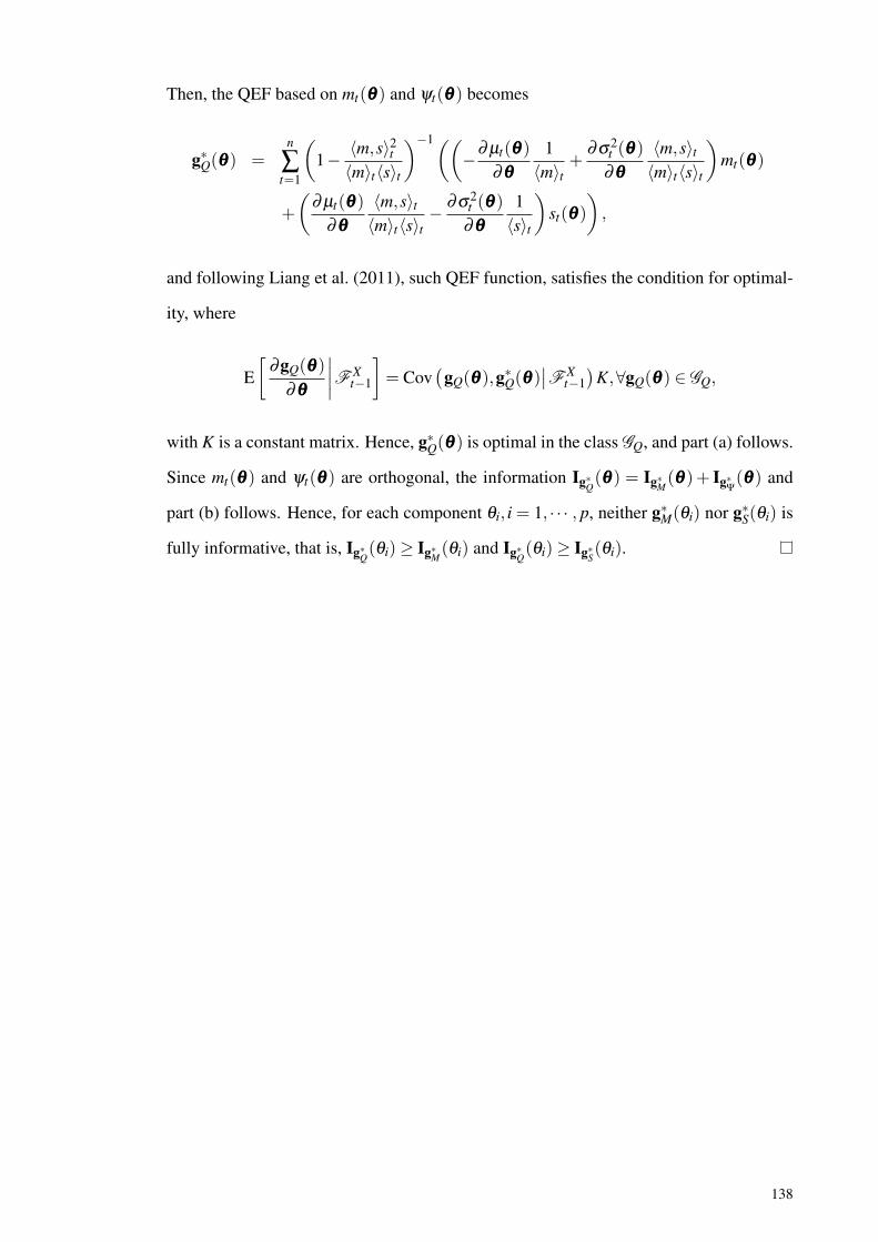
Then, the QEF based on mt(θθθ) and ψt(θθθ) becomes
g∗Q(θθθ) =n
∑t=1
(1− ⟨m,s⟩2
t⟨m⟩t⟨s⟩t
)−1((−∂ µt(θθθ)
∂θθθ1
⟨m⟩t+
∂σ2t (θθθ)
∂θθθ⟨m,s⟩t
⟨m⟩t⟨s⟩t
)mt(θθθ)
+
(∂ µt(θθθ)
∂θθθ⟨m,s⟩t
⟨m⟩t⟨s⟩t− ∂σ2
t (θθθ)∂θθθ
1⟨s⟩t
)st(θθθ)
),
and following Liang et al. (2011), such QEF function, satisfies the condition for optimal-
ity, where
E[
∂gQ(θθθ)∂θθθ
∣∣∣∣F Xt−1
]= Cov
(gQ(θθθ),g∗Q(θθθ)
∣∣F Xt−1)
K,∀gQ(θθθ) ∈ GQ,
with K is a constant matrix. Hence, g∗Q(θθθ) is optimal in the class GQ, and part (a) follows.
Since mt(θθθ) and ψt(θθθ) are orthogonal, the information Ig∗Q(θθθ) = Ig∗M(θθθ)+ Ig∗Ψ(θθθ) and
part (b) follows. Hence, for each component θi, i = 1, · · · , p, neither g∗M(θi) nor g∗S(θi) is
fully informative, that is, Ig∗Q(θi)≥ Ig∗M(θi) and Ig∗Q(θi)≥ Ig∗S(θi).
138